
BEAMING, SYNCHROTRON AND INVERSE COMPTONlabx.iasfbo.inaf.it/2014/resources/Ghisellini.pdf ·...
73
BEAMING, SYNCHROTRON AND INVERSE COMPTON Gabriele Ghisellini INAF – Osservatorio Astronomico di Brera September 13, 2008
Transcript of BEAMING, SYNCHROTRON AND INVERSE COMPTONlabx.iasfbo.inaf.it/2014/resources/Ghisellini.pdf ·...

BEAMING, SYNCHROTRON AND
INVERSE COMPTON
Gabriele Ghisellini
INAF – Osservatorio Astronomico di Brera
September 13, 2008

2

Contents
1 Beaming 5
1.1 Rulers and clocks . . . . . . . . . . . . . . . . . . . . . . . . . 5
1.2 Photographs and light curves . . . . . . . . . . . . . . . . . . 6
1.2.1 The moving bar . . . . . . . . . . . . . . . . . . . . . 6
1.2.2 The moving square . . . . . . . . . . . . . . . . . . . . 7
1.2.3 Rotation, not contraction . . . . . . . . . . . . . . . . 9
1.2.4 Time . . . . . . . . . . . . . . . . . . . . . . . . . . . . 10
1.2.5 Aberration . . . . . . . . . . . . . . . . . . . . . . . . 11
1.2.6 Intensity . . . . . . . . . . . . . . . . . . . . . . . . . . 12
1.2.7 Luminosity and flux . . . . . . . . . . . . . . . . . . . 13
1.2.8 Brightness Temperature . . . . . . . . . . . . . . . . . 16
1.2.9 Moving in an homogeneous radiation field . . . . . . . 16
1.3 A question . . . . . . . . . . . . . . . . . . . . . . . . . . . . . 19
2 Synchrotron emission and absorption 21
2.1 Introduction . . . . . . . . . . . . . . . . . . . . . . . . . . . . 21
2.2 Total losses . . . . . . . . . . . . . . . . . . . . . . . . . . . . 21
2.2.1 Synchrotron cooling time . . . . . . . . . . . . . . . . 25
2.3 Spectrum emitted by the single electron . . . . . . . . . . . . 25
2.3.1 Basics . . . . . . . . . . . . . . . . . . . . . . . . . . . 25
2.3.2 The real stuff . . . . . . . . . . . . . . . . . . . . . . . 26
2.3.3 Limits of validity . . . . . . . . . . . . . . . . . . . . . 29
2.3.4 From cyclotron to synchrotron emission . . . . . . . . 29
2.4 Emission from many electrons . . . . . . . . . . . . . . . . . . 30
2.5 Synchrotron absorption: photons . . . . . . . . . . . . . . . . 32
2.5.1 From thick to thin . . . . . . . . . . . . . . . . . . . . 34
2.6 Synchrotron absorption: electrons . . . . . . . . . . . . . . . . 35
3 Appendix: Useful Formulae 39
3.1 Synchrotron . . . . . . . . . . . . . . . . . . . . . . . . . . . . 39
3.1.1 Emissivity . . . . . . . . . . . . . . . . . . . . . . . . . 39
3.1.2 Absorption coefficient . . . . . . . . . . . . . . . . . . 40
3.1.3 Specific intensity . . . . . . . . . . . . . . . . . . . . . 41
3

4 CONTENTS
3.1.4 Self–absorption frequency . . . . . . . . . . . . . . . . 423.1.5 Synchrotron peak . . . . . . . . . . . . . . . . . . . . . 42
4 Compton scattering 43
4.1 Introduction . . . . . . . . . . . . . . . . . . . . . . . . . . . . 434.2 The Thomson cross section . . . . . . . . . . . . . . . . . . . 43
4.2.1 Why the peanut shape? . . . . . . . . . . . . . . . . . 444.3 Direct Compton scattering . . . . . . . . . . . . . . . . . . . . 464.4 The Klein–Nishina cross section . . . . . . . . . . . . . . . . . 47
4.4.1 Another limit . . . . . . . . . . . . . . . . . . . . . . . 494.4.2 Pause . . . . . . . . . . . . . . . . . . . . . . . . . . . 50
4.5 Inverse Compton scattering . . . . . . . . . . . . . . . . . . . 504.5.1 Thomson regime . . . . . . . . . . . . . . . . . . . . . 514.5.2 Typical frequencies . . . . . . . . . . . . . . . . . . . . 514.5.3 Cooling time and compactness . . . . . . . . . . . . . 564.5.4 Single particle spectrum . . . . . . . . . . . . . . . . . 57
4.6 Emission from many electrons . . . . . . . . . . . . . . . . . . 594.6.1 Non monochromatic seed photons . . . . . . . . . . . 60
4.7 Thermal Comptonization . . . . . . . . . . . . . . . . . . . . 624.7.1 Average number of scatterings . . . . . . . . . . . . . 624.7.2 Average gain per scattering . . . . . . . . . . . . . . . 624.7.3 Comptonization spectra: basics . . . . . . . . . . . . . 64
5 Synchrotron Self–Compton 69
5.1 SSC emissivity . . . . . . . . . . . . . . . . . . . . . . . . . . 695.2 Diagnostic . . . . . . . . . . . . . . . . . . . . . . . . . . . . . 715.3 Why it works . . . . . . . . . . . . . . . . . . . . . . . . . . . 72

Chapter 1
Beaming
1.1 Rulers and clocks
Special relativity taught us two basic notions: comparing dimensions andflow of times in two different reference frame, we find out that they differ. Ifwe measure a ruler at rest, and then measure the same ruler when is moving,we find that, when moving, the ruler is shorter. If we syncronize two clocksat rest, and then let one move, we see that the moving clock is delaying.Let us see how this can be derived by using the Lorentz transformations,connecting the two reference frames K (that sees the ruler and the clockmoving) and K ′ (that sees the ruler and the clock at rest). For semplicity,but without loss of generality, consider a a motion along the x axis, withvelocity v ≡ βc corresponding to the Lorentz factor Γ. Primed quantitiesare measured in K ′. We have:
x′ = Γ(x− vt)
y′ = y
z′ = z
t′ = Γ(
1 − βx
c
)
(1.1)
with the inverse relations given by
x = Γ(x′ + vt′)
y = y′
z = z′
t = Γ
(
t′ + βx′
c
)
. (1.2)
The length of a moving ruler has to be measured through the position of itsextremes at the same time t. Therefore, as ∆t = 0, we have
x′2 − x′1 = Γ(x2 − x1) − Γv∆t = Γ(x2 − x1) (1.3)
5

6 CHAPTER 1. BEAMING
i.e.
∆x =∆x′
Γ→ contraction (1.4)
Similarly, in order to determine a time interval a (lab) clock has to becompared with one in the comoving frame, which has, in this frame, the
same position x′. Then
∆t = Γ∆t′ + Γβ∆x′
c= Γ∆t′ → dilation (1.5)
An easy way to remember the transformations is to think to mesons pro-duced in collisions of cosmic rays in the high atmosphere, which can bedetected even is their lifetime (in the comoving frame) is much shorter thanthe time needed to reach the earth’s surface. For us, on ground, relativisticmesons live longer (for the meson’s point of view, instead, it is the length ofthe travelled disctance which is shorter).
All this is correct if we measure lengths by comparing rulers (at the sametime in K) and by comparing clocks (at rest in K ′) – the meson lifetime isa clock. In other words, if we do not use photons for the measurementprocess.
1.2 Photographs and light curves
If we have an extended moving object and if the information (about positionand time) are carried by photons, we must take into account their (different)travel paths. When we take a picture, we detect photons arriving at the sametime to our camera: if the moving body which emitted them is extended,we must consider that these photons have been emitted at different times,when the moving object occupied different locations in space. This mayseem quite obvious. And it is. Nevertheless these facts were pointed out in1959 (Terrel 1959; Penrose 1959), more than 50 years after the publicationof the theory of special relativity.
1.2.1 The moving bar
Let us consider a moving bar, of proper dimension ℓ′, moving in the directionof its length at velocity βc and at an angle θ with respect to the line of sight(see Fig. 1.1). The length of the bar in the frame K (according to relativity“without photons”) is ℓ = ℓ′/Γ. The photon emitted in A1 reaches thepoint H in the time interval ∆te. After ∆te the extreme B1 has reachedthe position B2, and by this time, photons emitted by the other extremeof the bar can reach the observer simultaneously with the photons emittedby A1, since the travel paths are equal. The length B1B2 = βc∆te, whileA1H = c∆te. Therefore
A1H = A1B2 cos θ → ∆te =ℓ′ cos θ
Γ(1 − β cos θ). (1.6)

1.2. PHOTOGRAPHS AND LIGHT CURVES 7
Figure 1.1: A bar moving with velocity βc in the direction of its length. Thepath of the photons emitted by the extreme A is longer than the path ofphotons emitted by B. When we make a picture of the bar (or a map), wecollect photons reaching the detector simultaneously. Therefore the photonsfrom A have to be emitted before those from B, when the bar occupiedanother position.
Note the appearance of the term δ = 1/[Γ(1−β cos θ)] in the transformation:this accounts for both the relativistic length contraction (1/Γ), and theDoppler effect [1/(1 − β cos θ)]. The length A1B2 is then given by
A1B2 =A1H
cos θ=
ℓ′
Γ(1 − β cos θ)= δℓ′. (1.7)
In a real picture, we would see the projection of A1B2, i.e.:
HB2 = A1B2 sin θ = ℓ′sin θ
Γ(1 − β cos θ)= ℓ′δ sin θ, (1.8)
The observed length depends on the viewing angle, and reaches the maxi-mum (equal to ℓ′) for cos θ = β.
1.2.2 The moving square
Now consider a square of size ℓ′ in the comoving frame, moving at 90 to theline of sight (Fig. 1.2). Photons emitted in A, B, C and D have to arrive
8 CHAPTER 1. BEAMING
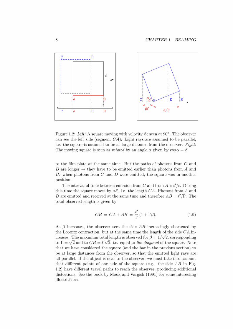
Figure 1.2: Left: A square moving with velocity βc seen at 90. The observercan see the left side (segment CA). Light rays are assumed to be parallel,i.e. the square is assumed to be at large distance from the observer. Right:
The moving square is seen as rotated by an angle α given by cosα = β.
to the film plate at the same time. But the paths of photons from C andD are longer → they have to be emitted earlier than photons from A andB: when photons from C and D were emitted, the square was in anotherposition.
The interval of time between emission from C and from A is ℓ′/c. Duringthis time the square moves by βℓ′, i.e. the length CA. Photons from A andB are emitted and received at the same time and therefore AB = ℓ′/Γ. Thetotal observed length is given by
CB = CA+AB =ℓ′
Γ(1 + Γβ). (1.9)
As β increases, the observer sees the side AB increasingly shortened bythe Lorentz contraction, but at the same time the length of the side CA in-creases. The maximum total length is observed for β = 1/
√2, corresponding
to Γ =√
2 and to CB = ℓ′√
2, i.e. equal to the diagonal of the square. Notethat we have considered the square (and the bar in the previous section) tobe at large distances from the observer, so that the emitted light rays areall parallel. If the object is near to the observer, we must take into accountthat different points of one side of the square (e.g. the side AB in Fig.1.2) have different travel paths to reach the observer, producing additionaldistortions. See the book by Mook and Vargish (1991) for some interestingillustrations.
1.2. PHOTOGRAPHS AND LIGHT CURVES 9
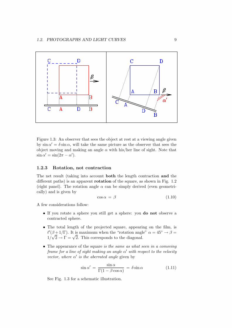
Figure 1.3: An observer that sees the object at rest at a viewing angle givenby sinα′ = δ sinα, will take the same picture as the observer that sees theobject moving and making an angle α with his/her line of sight. Note thatsinα′ = sin(2π − α′).
1.2.3 Rotation, not contraction
The net result (taking into account both the length contraction and thedifferent paths) is an apparent rotation of the square, as shown in Fig. 1.2(right panel). The rotation angle α can be simply derived (even geometri-cally) and is given by
cosα = β (1.10)
A few considerations follow:
• If you rotate a sphere you still get a sphere: you do not observe acontracted sphere.
• The total length of the projected square, appearing on the film, isℓ′(β+1/Γ). It is maximum when the “rotation angle” α = 45 → β =1/√
2 → Γ =√
2. This corresponds to the diagonal.
• The appearance of the square is the same as what seen in a comoving
frame for a line of sight making an angle α′ with respect to the velocity
vector, where α′ is the aberrated angle given by
sinα′ =sinα
Γ(1 − β cosα)= δ sinα (1.11)
See Fig. 1.3 for a schematic illustration.
10 CHAPTER 1. BEAMING
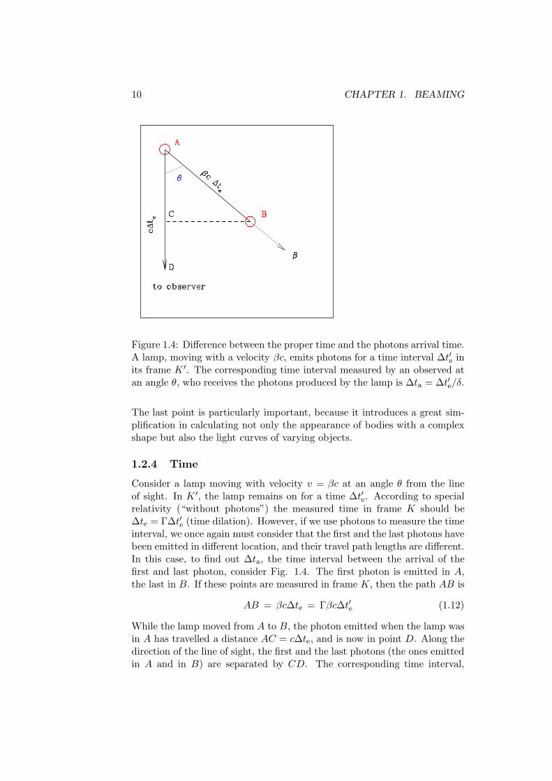
Figure 1.4: Difference between the proper time and the photons arrival time.A lamp, moving with a velocity βc, emits photons for a time interval ∆t′e inits frame K ′. The corresponding time interval measured by an observed atan angle θ, who receives the photons produced by the lamp is ∆ta = ∆t′e/δ.
The last point is particularly important, because it introduces a great sim-plification in calculating not only the appearance of bodies with a complexshape but also the light curves of varying objects.
1.2.4 Time
Consider a lamp moving with velocity v = βc at an angle θ from the lineof sight. In K ′, the lamp remains on for a time ∆t′e. According to specialrelativity (“without photons”) the measured time in frame K should be∆te = Γ∆t′e (time dilation). However, if we use photons to measure the timeinterval, we once again must consider that the first and the last photons havebeen emitted in different location, and their travel path lengths are different.In this case, to find out ∆ta, the time interval between the arrival of thefirst and last photon, consider Fig. 1.4. The first photon is emitted in A,the last in B. If these points are measured in frame K, then the path AB is
AB = βc∆te = Γβc∆t′e (1.12)
While the lamp moved from A to B, the photon emitted when the lamp wasin A has travelled a distance AC = c∆te, and is now in point D. Along thedirection of the line of sight, the first and the last photons (the ones emittedin A and in B) are separated by CD. The corresponding time interval,
1.2. PHOTOGRAPHS AND LIGHT CURVES 11
CD/c, is the interval of time ∆ta between the arrival of the first and thelast photon:
∆ta =CD
c=
AD −AC
c= ∆te − β∆te cos θ
= ∆te(1 − β cos θ)
= ∆t′eΓ(1 − β cos θ)
=∆t′eδ
(1.13)
If θ is small and the velocity is relativistic, then δ > 1, and ∆ta < ∆ts, i.e.we measure a time contraction instead of time dilation. Note also that werecover the usual time dilation (i.e. ∆ta = Γ∆t′e) if θ = 90, because in thiscase all photons have to travel the same distance to reach us.
Since a frequency is the inverse of time, it will transform as
ν = ν ′ δ (1.14)
It is because of this that the factor δ is called the relativistic Doppler factor.
1.2.5 Aberration
Another very important effect happening when a source is moving is theaberration of light. It is rather simple to understand, if one looks at Fig.1.5. A source of photons is located perpendilarly to the right wall of a lift.If the lift is not moving, and there is a hole in its right wall, then the ligthray enters in A and ends its travel in B. If the lift is not moving, A andB are at the same heigth. If the lift is moving with a constant velocityv to the top, when the photon smashes the right wall it has a differentlocation, and the point B will have, for a comoving observer, a smallerheight than A. The light ray path now appears oblique, tilted. Of course,the greater v, the more tilted the light ray path appears. This immediatelystimulate the question: what happens if the lift, instead to move with aconstant velocity, is accelerating? This this example one can easily convincehim/herself that the “trajectory” of the photon would appear curved. Since,by the equivalence principle, the accelerating lift cannot tell if there is anengine pulling him up or if there is a planet underneath it, we can then saythat gravity bends the light rays, and make the space curved.
This helps to understand why angles, between two inertial frames, change.Calling θ the angle between the direction of the emitted photon and thesource velocity vector, we have:
sin θ =sin θ′
Γ(1 + β cos θ′); sin θ′ =
sin θ
Γ(1 − β cos θ)
cos θ =cos θ′ + β
1 + β cos θ′; cos θ′ =
cos θ − β
1 − β cos θ(1.15)

12 CHAPTER 1. BEAMING
Figure 1.5: The relativistic lift, to explain relativistic aberration of light.Assume first a non–moving lift, with a hole on the right wall. A light ray,coming perpendiculrly to the left wall, enter through the wall in A and endsits travel in B. If the lift is moving with a constant velocity v to the top,its position is changed when the photon arrives to the left wall. For thecomoving observer, therefore, it appears that the light path is tilted, sincethe point B where the photon smashes into the left wall is below the pointA. What happens if the lift, instead to move with a constant velocity, isaccelerating?
Note that, if θ′ = 90, then sin θ = 1/Γ and cos θ = β. Consider a souceemitting isotropically in K ′. Halph of its photons are emitted in the emi-sphere, namely, with θ′ ≤ 90. Then, in K, the same source will appear toemit halph of its photons into a cone of semiaperture Γ.
Assuming symmetry around the angle φ, the transformation of the solidangle dΩ is
dΩ = 2πd cos θ =dΩ′
Γ2(1 + β cos θ′)2= dΩ′ Γ2(1 − β cos θ)2 =
dΩ′
δ2(1.16)
1.2.6 Intensity
We now have all the ingredients necessary to calculate the transformationof the specific (i.e. monochromatic) and bolometric intensity. The specificintensity has the unit of energy per unit surface, time, frequency and solidangle. In cgs, the units are [erg cm−2 s−1 Hz−1 ster−1]. We can then write

1.2. PHOTOGRAPHS AND LIGHT CURVES 13
the specific intensity as
I(ν) = hνdN
dt dν dΩ dA
= δhν ′dN ′
(dt′/δ) δdν ′ (dΩ′/δ2) dA′
= δ3 I ′(ν ′) = I ′(ν/δ) (1.17)
Note that dN = dN ′ because it is a number, and that dA = dA′ because itis an area perpendicular to the velocity. If we integrate over frequencies weobtain the bolometric intensity which transforms as
I = δ4I ′ (1.18)
The fourth power of δ can be understood in a simple way: one power comesfrom the transformation of the frequencies, one for the time, and two forthe solid angle. They all add up. This transformation is at the base of ourunderstanding of relativistic sources, namely radio–loud AGNs, gamma–raybursts and galactic superluminal sources.
1.2.7 Luminosity and flux
The transformation of fluxes and luminosities from the comoving to theobserver frames is not trivial. The most used formula is L = δ4L′, but thisassumes that we are dealing with a single, spherical blob. It can be simplyderived by noting that L = 4πd2
LF , where F is the observed flux, and byconsidering that the flux, for a distance source, is F ∝
∫
ΩsIdΩ. Since Ωs is
the source solid angle, which is the same in the two K and K ′ frames, wehave that F transforms like I, and so does L. But the emission from jetsmay come not only by a single spherical blob, but by, for instance, manyblobs, or even by a continuos distribution of emitting particles flowing inthe jet. If we assume that the walls of the jet are fixed, then the concept of“comoving” frame is somewhat misleading, because if we are comoving withthe flowing plasma, then we see the walls of the jet which are moving.
A further complication exists if the velocity is not uni–directional, butradial, like in gamma–ray bursts. In this case, assume that the plasma iscontained in a conical narrow shell (width smaller than the distance of theshell from the apex of the cone). The observer which is moving togetherwith a portion of the plasma, (the nearest case of a “comoving observer”)will see the plasma close to her going away from her, and more so for moredistant portions of the plasma. Indeed, there could be a limiting distancebeyond which the two portions of the shells are causally disconnected.
Useful references are Lind & Blandford (1985) and Sikora et al. (1997).The (frequency integrated) emissivity j is the energy emitted per unit
time, solid angle and volume. We generally have that the intensity, for an

14 CHAPTER 1. BEAMING
otpically thin source, is I =∫
∆R jdr, where ∆R is the length of the regioncontaining the emitting particles. This quantity transforms like j = j′δ3,namely with one power of δ less than the intensity.
Figure 1.6: Due to aberration of light, the travel path of the a light ray isdifferent in the two frames K and K ′
To understand why, consider a slab with plasma flowing with a velocityparallel to the walls of the slab, as in Fig. 1.6. The observer in K willmeasure a certain ∆R which depends on her viewing angle. In K ′ the samepath has a different length, because of the aberration of light. The heightof the slab h′ = h, since it is perpendicular to the velocity. The light raytravels a distance ∆R = h/ sin θ in K, and the same light ray travels adistance ∆R′ = h′/ sin θ′ in K ′. Since sin θ′ = sin θδ, then ∆R′ = δR/δ.Therefore the column of plasma contributing to the emission, for δ > 1,is less than what the observer in K would guess by measuring ∆R. Forsemplicity, assume that the plasma is homogenous, allowing to simply writeI = j∆R. In this case:
I = j∆R = δ4I ′ = δ4j′∆R′ → j = δ3j′ (1.19)
And the corresponding transformation for the specific emissivity is j(ν) =δ2j′(ν ′).
Fig. 1.7 illustrates another interesting example, taken from the workof Sikora et al. (1997). Consider that within a distance R from the apexof a jet (R measured in K), at any given time there are N blobs (10 onthe specific example of Fig. 1.7), moving with a velocity v = βc along thejet. To fix the ideas, let assume that beyond R they switch off. If theviewing angle is θ = 90, the photons emitted by each blob travel the samedistance to reach the observer, who will see all the 10 blobs. But if θ < 90,the photons produced by the rear blobs must travel for a longer distance in

1.2. PHOTOGRAPHS AND LIGHT CURVES 15
Figure 1.7: Due to the differences in light travel time, the number of blobsthat can be observed simultaneously at any given time depends on the view-ing angle and the velocity of the blobs. In the top panel the viewing angleis θ = 90 and all the blobs contained within a certain distance R can beseen. For smaller viewing angles, less blobs are seen. This is because thephotons emitted by the rear blobs have more distance to travel, and there-fore they have to be emitted before the photons produced by the front blob.Decreasing the viewing angle θ we see less blobs (3 for the case illustratedin the bottom panel).
order to reach the observer, and therefore they have to be emitted before thephotons produced by the front blob. The observer will then see less blobs.To be more quantitative, consider a viewing angle θ < 90. Photons emittedby blob numer 3 to reach blobs number 1 when it produces its last photon(before to switch off) were emitted when the blobs itself was just born (it wascrossing point A). They travelled a distance R cos θ in a time ∆t. Duringthe same time, the blob number 3 travelled a distance ∆R = cβ∆t in theforward direction. The fraction f of blobs that can be seen is then
f =R− ∆R
R= 1 − cβ∆t
R= 1 − β cos θ (1.20)
Where we have used the fact that ∆t = (R/c) cos θ. This is the usualDoppler factor. We may multiply and divide by Γ to obtain
f =1
Γδ(1.21)
16 CHAPTER 1. BEAMING
The bottom line is the following: even if the flux from a single blob is boostedby δ4, if the jet is made by many (N) equal blobs, the total flux is not justboosted by Nδ4 times the intrinsic flux of a blob, because the observer willsee less blobs if θ < 90.
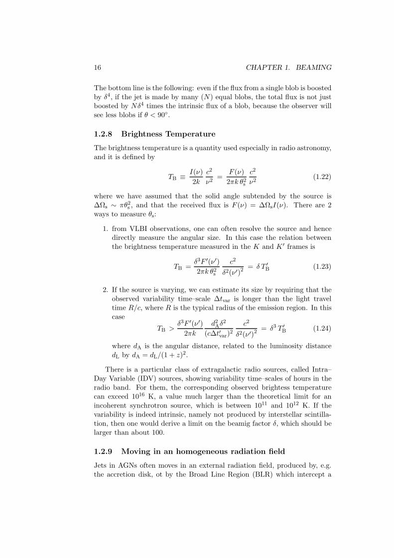
1.2.8 Brightness Temperature
The brightness temperature is a quantity used especially in radio astronomy,and it is defined by
TB ≡ I(ν)
2k
c2
ν2=
F (ν)
2πk θ2s
c2
ν2(1.22)
where we have assumed that the solid angle subtended by the source is∆Ωs ∼ πθ2
s , and that the received flux is F (ν) = ∆ΩsI(ν). There are 2ways to measure θs:
1. from VLBI observations, one can often resolve the source and hencedirectly measure the angular size. In this case the relation betweenthe brightness temperature measured in the K and K ′ frames is
TB =δ3F ′(ν ′)
2πk θ2s
c2
δ2(ν ′)2= δ T ′
B (1.23)
2. If the source is varying, we can estimate its size by requiring that theobserved variability time–scale ∆tvar is longer than the light traveltime R/c, where R is the typical radius of the emission region. In thiscase
TB >δ3F ′(ν ′)
2πk
d2Aδ
2
(c∆t′var)2
c2
δ2(ν ′)2= δ3 T ′
B (1.24)
where dA is the angular distance, related to the luminosity distancedL by dA = dL/(1 + z)2.
There is a particular class of extragalactic radio sources, called Intra–Day Variable (IDV) sources, showing variability time–scales of hours in theradio band. For them, the corresponding observed brightess temperaturecan exceed 1016 K, a value much larger than the theoretical limit for anincoherent synchrotron source, which is between 1011 and 1012 K. If thevariability is indeed intrinsic, namely not produced by interstellar scintilla-tion, then one would derive a limit on the beamig factor δ, which should belarger than about 100.
1.2.9 Moving in an homogeneous radiation field
Jets in AGNs often moves in an external radiation field, produced by, e.g.the accretion disk, ot by the Broad Line Region (BLR) which intercept a

1.2. PHOTOGRAPHS AND LIGHT CURVES 17
fraction of the radiation produved by the disk and re–emit it in the formof emission lines. It it therefore interesting to calculate what is the energydensity seen by a an observer which is comoving with the jet plasma.
Figure 1.8: A real case: a relativistic bob is moving with the Broad LineRegion of a radio loud AGN, with Lorentz factor Γ. In the rest frame K ′ ofthe blob the photons coming from 90 in frame K are seen to come at anangle 1/Γ. The energy density as seen by the blob is enhanced by a factor∼ Γ2.
To make a specific example, as illistrated bu Fig. 1.8, assume that aportion of the jet is moving with a bulk Lorentz factor Γ, velocity βc andthat it is surrounded by an shell of broad line clouds. For simplicity, assumethat the broad line photons are produced by the surface of a sphere ofradius R and that the jet is within it. Assume also that the radiation ismonochromatic at sum frequency ν0 (in frame K). The comoving (in frameK ′) observer will see photons coming from an emisphere (the other half maybe hidden by the accretion disk): photons coming from the forward directionare seen blue-shifted by a factor (1 + β)Γ, while photons that the observerin K sees as coming from the side (i.e. 90 degrees) will be observed in K ′
as coming by an angle given by sin θ′ = 1/Γ (and cos θ′ = β) and will beblue–shifted by a factor Γ. As seen in K ′, each element of the BLR surface is

18 CHAPTER 1. BEAMING
moving in the opposite direction of the actual jet velocity, and the photonsemitted by this element form an angle θ′ with respect the element velocity.The Doppler factor used by K ′ is then
δ′ =1
Γ(1 − β cos θ′)(1.25)
The intensity coming from each element is seen boosted as (cfr Eq. 1.2.9):
I ′ = δ′4I (1.26)
The radiation energy density is the integral over the solid angle of the in-tensity, divided by c:
U ′ =2π
c
∫ 1
βI ′d cos θ′
=2π
c
∫ 1
β
I
Γ4(1 − β cos θ′)4d cos θ′
=
(
1 + β +β2
3
)
Γ2 2πI
c
=
(
1 + β +β2
3
)
Γ2 U (1.27)
Note that the limits of the integral correspond to the angles 0′ and 90 inframe K. The radiation energy density, in frame K ′, is then boosted by afactor (7/3)Γ2 when β ∼ 1. Doing the same calculation for a sphere, onewould obtain U ′ = Γ2U .
Furthermore a (monochromatic) flux in K is seen, in K ′, at differentfrequencies, between Γν0 and (1 + β)Γν0, with a slope F ′(ν ′) ∝ ν ′2. Whythe slope ν ′2? This can be derived as follows: we already know that I ′(ν ′) =δ′3I(ν) = (ν ′/ν)3I(ν). The flux at a specific frequency is
F ′(ν ′) = 2π
∫ µ′
2
µ′
1
dµ′(
ν ′
ν
)3
I(ν) (1.28)
where µ′ ≡ cos θ′, and the integral is over those µ′ contributing at ν ′. Since
ν ′
ν= δ′ =
1
Γ(1 − βµ′)→ µ′ =
1
β
(
1 − ν
Γν ′
)
(1.29)
we have
dµ′ = − dν
βΓν ′(1.30)
Therefore, if the intensity is monochromatic in frame K, i.e. I(ν) = I0δ(ν−ν0), the flux density in the comoving frame is
F ′(ν ′) = 2π
∫ ν1
ν2
dν
βΓν ′
(
ν ′
ν
)3
I0δ(ν − ν0)
=2π
Γβ
I0ν30
ν ′2; Γν0 ≤ ν ′ ≤ (1 + β)Γν0 (1.31)

1.3. A QUESTION 19
where the frequency limits corresponds to photons produced in an emispherein frame K, and between 0 and sin θ′ = 1/Γ in frame K ′. Integrating Eq.2.25 over frequency, one obtains
F ′ = 2πI0Γ2
(
1 + β +β2
3
)
= Γ2
(
1 + β +β2
3
)
F (1.32)
in agreement with Eq. 1.27.
ν = ν ′δ frequencyt = t′/δ timeV = V ′δ volumesin θ = sin θ′/δ sinecos θ = (cos θ′ + β)/(1 + β cos θ′) cosineI(ν) = δ3I ′(ν ′) specific intensityI = δ4I ′ total intensityj(ν) = j′(ν ′)δ2 specific emissivityκ(ν) = κ′(ν ′)/δ absorption coefficientTB = T ′
Bδ brightn. temp. (size directly measured)TB = T ′
Bδ3 brightn. temp. (size from variability)
Table 1.1: Useful relativistic transformations
1.3 A question
Suppose that some plasma of mass m is falling onto a central object with avelocity v and bulk Lorentz factor Γ. The central object has mass M andproduces a luminosity L. Assume that the interaction is through Thomsonscattering and that there are no electron–positron pairs.
a) What is the radiation force acting on the electron?b) What is the gravity force acting on the proton?c) What definition of limiting (“Eddington”) luminosity would you give
in this case?d) What happens if the plasma is instead going outward?
References
Lind K.R. & Blandford R.D., 1985, ApJ, 295, 358Mook D.E. & Vargish T., 1991, Inside Relativity, Princeton Univ. PressSikora M., Madejski G., Moderski R. & Poutanen J., 1997, ApJ, 484,
108

20 CHAPTER 1. BEAMING

Chapter 2
Synchrotron emission and
absorption
2.1 Introduction
We now know for sure that many astrophysical sources are magnetized andhave relativistic leptons. Magnetic field and relativistic particles are the twoingredients to have synchrotron radiation. What is responsible for this kindof radiation is the Lorentz force, making the particle to gyrate around themagnetic field lines. Curiously enough, this force does not work, but makesthe particles to accelerate even if their velocity modulus hardly changes.
The outline of this section is:
1. We will derive the total power emitted by the single electron. Totalmeans integrated over frequency and over emission angles. This willrequire to generalize the Larmor formula to the relativistic case;
2. We will then outline the basics of the spectrum emitted by the singleelectron. This is treated is several text–books, so we will concentrateon the basic concepts;
3. Spectrum from an ensemble of electrons. Again, only the basics;
4. Synchrotron self absorption. We will try to discuss things from thepoint of view of a photon, that wants to calculate its survival proba-bility, and also the point of view of the electron, that wants to calculatethe probability to absorb the photon, and then increase its energy andmomentum.
2.2 Total losses
To calculate the total (=integrated over frequencies and emission angles)synchrotron losses we go into the frame that is instantaneously at rest with
21

22 CHAPTER 2. SYNCHROTRON EMISSION AND ABSORPTION
the particle (in this frame v is zero, but not the acceleration!). This isbecause we will use the fact that the emitted power is Lorentz invariant:
Pe = P ′e =
2e2
3c3a′2 =
2e2
3c3
[
a′2‖ + a′2⊥
]
(2.1)
where the subscript “e” stands for “emitted”. The fact that the power isinvariant sounds natural, since after all, power is energy over time, and bothenergy and time transforms the same way (in special relativity with rulersand clocks). But be aware that this does not mean that the emitted andreceived power are the same. They are not!
The problem is now to find how the parallel (to the velocity vector) andperpendicular components of the acceleration Lorentz transform. This isdone in text books, so we report the results:
a′‖ = γ3a‖
a′⊥ = γ2a⊥ (2.2)
where γ is the particle Lorentz factor. One easy way to understand and re-member these transformations is to recall that the acceleration is the secondderivative of space with respect to time. The perpendicular component ofthe displacement is invariant, so we have only to transform (twice) the time(factor γ2). The parallel displacement instead transforms like γ, hence theγ3 factor.
The generalization of the Larmor formula is then:
Pe = P ′e =
2e2
3c3
[
a′2‖ + a′2⊥
]
=2e2
3c3γ4
[
γ2a2‖ + a2
⊥
]
(2.3)
Don’t be fooled by the γ2 factor in front of a2‖... this component of the power
is hardly important: since the velocity, for relativistic particles, is alwaysclose to c, it implies that one can get very very small acceleration in the samedirection of the velocity. This is why linear accelerators minimize radiationlosses. For synchrotron machines, instead, the losses due to radiation can bethe limiting factor, and they are of course due to a⊥: changing the direction
of the velocity means large accelerations, even without any change in thevelocity modulus. To go further, we have to calculate the two component ofthe acceleration for an electron moving in a magnetic field. Its trajectory,in general, will have an helical shape of radius rL (the Larmor radius). Theangle that the velocity vector makes with the magnetic field line is calledpitch angle. Let us denote it with θ. We can anticipate that, in the absenceof electric field and for a homogeneous magnetic field, the modulus of thevelocity will not change: the magnetic field does not work, and so there isno change of energy, except for the losses due to the synchrotron radiationitself. So one important assumption is that at least during one gyration, the

2.2. TOTAL LOSSES 23
Figure 2.1: A particle gyrates along the magnetic field lines. Its trajectoryhas an helicoidal shape, with Larmor radius rL and pitch angle θ.
losses are not important. This is almost always satisfied in astrophysicalsettings, but there are indeed some cases where this is not true.
When there is no electric field the only acting force is the (relativistic)Lorentz force:
FL =d
dt(γmv) =
e
cv ×B (2.4)
The parallel and perpendicular components are
FL‖ = e v‖B = 0 → a‖ = 0
FL⊥ = γmdv⊥dt
= ev⊥cB → a⊥ =
evB sin θ
γmc(2.5)
We can also derive the Larmor radius rL by setting a⊥ = v2⊥/rL, and so
rL =v2⊥
a⊥=
γmc2β sin θ
eB(2.6)
The fundamental frequency is the inverse of the time occurring to completeone orbit (gyration frequency), so νB = cβ sin θ/(2πrL), giving
νB =eB
2πγmc=
νL
γ(2.7)

24 CHAPTER 2. SYNCHROTRON EMISSION AND ABSORPTION
where νL is the Larmor frequency, namely the gyration frequency for sub–relativistic particles. Larger B means smaller rL, hence greater gyrationfrequencies. Vice–versa, larger γ means larger inertia, thus larger rL, andsmaller gyration frequencies. Substituting a⊥ given in Eq. 2.5 in the gener-alized Larmor formula (Eq. 2.3) we get:
PS =2e4
3m2c3B2γ2β2 sin2 θ (2.8)
We can make it nicer (for future use) by recalling that:
• The magnetic energy density is UB ≡ B2/(8π)
• the quantity e2/(mec2), in the case of electrons, is the classical electron
radius r0
• the square of the electron radius is proportional to the Thomson scat-tering cross section σT, i.e. σT = 8πr20/3 = 6.65 × 10⁻²⁵ cm2.
Making these substitutions, we have that the synchrotron power emitted bya single electron of given pitch angle is:
PS(θ) = 2σTcUBγ2β2 sin2 θ (2.9)
In the case of an isotropic distribution of pitch angles we can average theterm sin2 θ over the solid angle. The result is 2/3, giving
〈PS〉 =4
3σTcUBγ
2β2 (2.10)
Now pause, and ask yourself:
• Is PS valid only for relativistic particles, or does it describe correctlythe radiative losses also for sub–relativistic ones?
• In the relativistic case the losses are proportional to the square of theelectron energy. Do you understand why? And for sub–relativisticparticles?
• What happens of we have protons, instead of electrons?
• What happens for θ → 0? Are you sure? (that losses vanishes..). Ok,but what happens to the received power when you have the lines ofthe magnetic field along the line of sight, and a beam of particles, allwith a small pitch angles, shooting at you?
• Why on earth there is the scattering cross section? Is this a coincidenceor does it hide a deeper fact?

2.3. SPECTRUM EMITTED BY THE SINGLE ELECTRON 25
2.2.1 Synchrotron cooling time
When you want to estimate a timescale of a quantity A, you can alwayswrite t = A/A. In our case A is the energy of the particle. For electronswith an isotropic pitch angle distribution we have
tsyn =E
〈PS〉=
γmec2
(4/3)σTcUBγ2β2∼ 7.75 × 10⁸
B2γs =
24.57
B2γyr (2.11)
In the vicinity of a supermassive AGN black hole we can have B = 103B3
Gauss and γ = 103γ3, yielding tsyn = 0.75/(B23γ3) s. The same electron, in
the radio lobes of a radio loud quasars with B = 10−5B−5 Gauss, cools intsyn = 246 million years.
2.3 Spectrum emitted by the single electron
2.3.1 Basics
There exists a typical frequency associated to the synchrotron process. Thisis related to the inverse of a typical time. If the electron is relativistic, thisis not the revolution period. Instead, it is the fraction of the time, for eachorbit, during which the observer receives some radiation. To simplify, con-sider an electron with a pitch angle of 90, and look at Fig. 2.2, illustratingthe typical patterns of the produced radiation for sub–relativistic electronsmoving with a velocity parallel (top panel) or perpendicular (mid panel) tothe acceleration. In the bottom panel we see the pattern for a relativisticelectron (with v ⊥ a): it is strongly beamed in the forward direction. This isthe direct consequence of the aberration of light, making half of the photonsbe emitted in a cone of semi–aperture angle 1/γ (which is called the beaming
angle). Note that this does not mean that half of the power is emitted within1/γ, because the photons inside the beaming cone are more energetic thanthose outside, and are more tightly packed (do you remember the δ4 factorwhen studying beaming?).
To go further, recall what we do when we study a time series and wewant to find the power spectrum: we Fourier transform it. In this case wemust do the same. Therefore if there is a typical timescale during which wereceive most of the signal, we can say that most of the power is emitted ata frequency that is the inverse of that time.
Look at Fig. 2.3: the relativistic electron emits photons all along itsorbit, but it will “shoot” in a particular direction only for the time
∆te ∼ AB
v=
2πrL2γv
=2
γνB(2.12)
where we made use of the the definition νB ≡ v/(2πrL). This is the emitting
time during which the electron emits photons that will reach the observer.
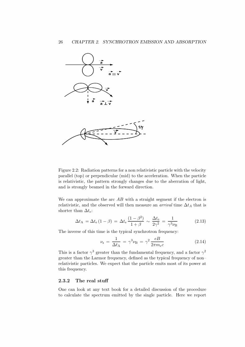
26 CHAPTER 2. SYNCHROTRON EMISSION AND ABSORPTION
Figure 2.2: Radiation patterns for a non relativistic particle with the velocityparallel (top) or perpendicular (mid) to the acceleration. When the particleis relativistic, the pattern strongly changes due to the aberration of light,and is strongly beamed in the forward direction.
We can approximate the arc AB with a straight segment if the electron isrelativistic, and the observed will then measure an arrival time ∆tA that isshorter than ∆te:
∆tA = ∆te (1 − β) = ∆te(1 − β2)
1 + β∼ ∆te
2γ2=
1
γ3νB(2.13)
The inverse of this time is the typical synchrotron frequency:
νs =1
∆tA= γ3νB = γ2 eB
2πmec(2.14)
This is a factor γ3 greater than the fundamental frequency, and a factor γ2
greater than the Larmor frequency, defined as the typical frequency of non–relativistic particles. We expect that the particle emits most of its power atthis frequency.
2.3.2 The real stuff
One can look at any text book for a detailed discussion of the procedureto calculate the spectrum emitted by the single particle. Here we report

2.3. SPECTRUM EMITTED BY THE SINGLE ELECTRON 27
Figure 2.3: A relativistic electron is gyrating along a magnetic field linewith pitch angle 90. Its trajectory is then a circle of radius rL. Due toaberration, an observer will “see it” (i.e. will measure an electric field)when the beaming cone of total aperture angle 2/γ is pointing at him.
the results: the power per unit frequency emitted by an electron of givenLorentz factor and pitch angle is:
Ps(ν, γ, θ) =
√3e3B sin θ
mec2F (ν/νc)
F (ν/νc) ≡ ν
νc
∫ ∞
ν/νc
K5/3(y)dy
νc ≡ 3
2νs sin θ (2.15)
This is the power integrated over the emission pattern. K5/3(y) is themodified Bessel function of order 5/3. The dependence upon frequencyis contained in F (ν/νc), that is plotted in Fig. 2.4. This function peaks atν ∼ 0.29νc, therefore very close to what we have estimated before, in ourvery approximate treatment. The low frequency part is well approximatedby a power law of slope 1/3:
F (ν/νc) → 4π√3Γ(1/3)
(
ν
2νc
)1/3
(ν ≪ νc) (2.16)
At ν ≫ νc the function decays exponentially, and can be approximated by:
F (ν/νc) →(π
2
)1/2(
ν
νc
)1/2
e−ν/νc (ν ≫ νc) (2.17)

28 CHAPTER 2. SYNCHROTRON EMISSION AND ABSORPTION
Figure 2.4: Top panel: The function F (ν/νc) describing the synchrotronspectrum emitted by the single electron. Bottom panel: F (ν/νc) is com-pared with some approximating formulae, as labeled. We have definedx ≡ ν/νc.

2.3. SPECTRUM EMITTED BY THE SINGLE ELECTRON 29
Another approximation valid for all frequency, but overestimating F aroundthe peak, is:
F (ν/νc) ∼ 4π√3Γ(1/3)
(
ν
2νc
)1/3
e−ν/νc (2.18)
2.3.3 Limits of validity
One limit can be obtained by requiring that, during one orbit, the emittedenergy is much smaller than the electron energy. If not, the orbit is modified,and our calculations are no more valid. For non–relativistic electrons thistranslates in demanding that
hνB < mec2 → B <
2πm2ec
3
he≡ Bc (2.19)
where Bc ∼ 4.4×10¹³ Gauss is the critical magnetic field, around and abovewhich quantum effects appears (i.e. quantized orbits, Landau levels and soon).
For relativistic particles we demand that the energy emitted during oneorbit does not exceed the energy of the particle.
Ps
νB< γmec
2 → B <e/σT
γ2 sin2 θ∼ 7.22 × 10¹⁴
γ2 sin2 θGauss (2.20)
Therefore for large γ we reach the validity limit even if the magnetic field issub–critical.
For very small pitch angles beware that the spectrum is not describedby F (ν/νc), but consists of a blue-shifted cyclotron line. This is because, inthe gyroframe, the particle is sub–relativistic, and so it emits only one (orvery few) harmonics, that the observer sees blueshifted.
2.3.4 From cyclotron to synchrotron emission
A look at Fig. 2.5 helps to understand the difference between cyclotronand synchrotron emission. When the particle is very sub–relativistic, theobserved electric field is sinusoidal in time. Correspondingly, the Fouriertransform of E(t) gives only one frequency, the first harmonic. Increasingsomewhat the velocity (say, β ∼ 0.01) the emission pattern starts to beasymmetric (for light aberration) and as a consequence E(t) must be de-scribed by more than just one sinusoid, and higher order harmonics appear.In these cases the ratio of the power contained in successive harmonics goesas β2.
Finally, for relativistic (i.e. γ ≫ 1) particles, the pattern is so asym-metric that the observers sees only spikes of electric field. They repeatthemselves with the gyration period, but all the power is concentrated into∆tA. To reproduce E(t) in this case with sinusoids requires a large number
30 CHAPTER 2. SYNCHROTRON EMISSION AND ABSORPTION
of them, with frequencies going at least up to 1/∆tA. In this case the har-monics are many, guaranteeing that the spectrum becomes continuous withany reasonable line broadening effect, and the power is concentrated at highfrequencies.
2.4 Emission from many electrons
Again, this problem is treated in several text books, so we repeat the basicresults using some approximations, tricks and shortcuts.
The queen of the particle energy distributions in high energy astrophysicsis the power law distribution:
N(γ) = K γ−p = N(E)dE
dγ; γminγ < γmax (2.21)
Now, assuming that the distribution of pitch angles is the same at low andhigh γ, we want to obtain the synchrotron emissivity produced by these par-ticles. Beware that the emissivity is the power per unit solid angle producedwithin 1 cm3. The specific emissivity is also per unit of frequency. So, if Eq.2.21 represents a density, we should integrate over γ the power produced bythe single electron (of a given γ) times N(γ), and divide all it by 4π, if theemission is isotropic:
ǫs(ν, θ) =1
4π
∫ γmax
γmin
N(γ)P (γ, ν, θ)dγ (2.22)
Doing the integral one easily finds that, in an appropriate range of frequen-cies:
ǫs(ν, θ) ∝ KB(p+1)/2ν−(p−1)/2 (2.23)
The important thing is that a power law electron distribution produces apower law spectrum, and the two spectral indices are related. We tradition-ally call α the spectral index of the radiation, namely ǫs ∝ ν−α. We thenhave
α =p− 1
2(2.24)
This result is so important that it is worth to try to derive it in a way assimple as possible, even without doing the integral of Eq. 2.22. We canin fact use the fact that the synchrotron spectrum emitted by the singleparticle is peaked. We can then say, without being badly wrong, that allthe power is emitted at the typical synchrotron frequency:
νs = γ2νL; νL ≡ eB
2πmec(2.25)
In other words, there is a tight correspondence between the energy of theelectron and the frequency it emits. To simplify further, let us assume that

2.4. EMISSION FROM MANY ELECTRONS 31
Figure 2.5: From cyclo to synchro: if the emitting particle has a very smallvelocity, the observer sees a sinusoidal (in time) electric field E(t). Increas-ing the velocity the pattern becomes asymmetric, and the second harmonicappears. For 0 < β ≪ 1 the power in the second harmonic is a factor β2 lessthan the power in the first. For relativistic particles, the pattern becomesstrongly beamed, the emission is concentrated in the time ∆tA. As a con-sequence the Fourier transformation of E(t) must contain many harmonics,and the power is concentrated in the harmonics of frequencies ν ∼ 1/∆tA.Broadening of the harmonics due to several effects ensures that the spec-trum in this case becomes continuous. Note that the fundamental harmonicbecomes smaller increasing γ (since νB ∝ 1/γ).

32 CHAPTER 2. SYNCHROTRON EMISSION AND ABSORPTION
the pitch angle is 90. The emissivity at a given frequency, within an intervaldν, is then the result of the emission of electrons having the appropriateenergy γ, within the interval dγ
ǫs(ν)dν =1
4πPsN(γ)dγ; γ =
(
ν
νL
)1/2
;dγ
dν=ν−1/2
2ν1/2L
(2.26)
we then have
ǫs(ν) ∝ B2γ2Kγ−pdγ
dν
∝ B2K
(
ν
νL
)(2−p)/2 ν−1/2
ν1/2L
∝ KB(p+1)/2 ν−(p−1)/2 (2.27)
where we have used νL ∝ B.
The synchrotron flux received from a homogeneous and thin source ofvolume V ∝ R3, at a distance dL, is
Fs(ν) = 4πǫs(ν)V
4πd2L
∝ R3
d2L
KB1+αν−α
∝ θ2sRKB
1+αν−α (2.28)
where θs is the angular radius of the source (not the pitch angle!). Observingthe source at two different frequencies allows to determine α, hence the slopeof the particle energy distribution. Furthermore, if we know the distanceand R, the normalization depends on the particle density and the magneticfield: two unknowns and only one equation. We need another relation toclose the system. As we will see in the following, this is provided by theself–absorbed flux.
2.5 Synchrotron absorption: photons
All emission processes have their absorption counterpart, and the synchrotronemission is no exception. What makes synchrotron special is really the factthat it is done by relativistic particles, and they are almost never distributedin energy as a Maxwellian. If they were, we could use the well known factthat the ratio between the emissivity and the absorption coefficient is equalto the black body (Kirchhoff law) and then we could easily find the absorp-tion coefficient. But in the case of a non–thermal particle distribution wecannot do that. Instead we are obliged to go back to more fundamental

2.5. SYNCHROTRON ABSORPTION: PHOTONS 33
relations, the one between the A and B Einstein coefficients relating spon-taneous and stimulated emission and “true” absorption (by the way, recallthat the absorption coefficient is what remains subtracting stimulated emis-sion from “true” absorption). But we once again will use some tricks, inorder to be as simple as possible. These are the steps:
1. The first trick is to think to our power law energy distribution as asuperposition of Maxwellians, of different temperatures. So, we willrelate the energy γmec
2 of a given electron to the energy kT of aMaxwellian.
2. We have already seen that there is a tight relation between the emittedfrequency and γ. Since the emission and absorption processes arerelated, we will assume that a particular frequency ν is preferentiallyabsorbed by those electrons that can emit it.
3. As a consequence, we can associate our “fake” temperature to thefrequency:
kT ∼ γmec2 ∼ mec
2
(
ν
νL
)1/2
(2.29)
4. For an absorbed source the brightness temperature Tb, defined by
I(ν) ≡ 2kTbν2
c2(2.30)
must be equal to the kinetic “temperature” of the electrons, and so
I(ν) ≡ 2kTν2
c2∼ 2me ν
2
(
ν
νL
)1/2
∝ ν5/2
B1/2(2.31)
These are the right dependencies. Note that the spectrum is ∝ ν5/2, notν2, and this is the consequence of having “different temperatures”. Notealso that the particle density disappeared: if you think about it is natural:the more electrons you have, the more you emit, but the more you absorb.Finally, even the slope of the particle distribution is not important, it controls(up to a factor of order unity) only the normalization of I(ν) (our ultra–simple derivation cannot account for it, see the Appendix).
The above is valid as long as we can associate a specific γ to any ν.This is not always the case. Think for instance to a cut–off distribution,with γmin ≫ 1. In this case the electrons with γmin are the most efficientemitters and absorbers of all photons with ν < νmin ≡ γ2
minνL. So in this casewe should not associate a different temperature when dealing with different

34 CHAPTER 2. SYNCHROTRON EMISSION AND ABSORPTION
Figure 2.6: The synchrotron spectrum from a partially self absorbed source.Observations of the self absorbed part could determine B. Observations ofthe thin part can then determine K and the electron slope p.
ν < νmin. But if do not change T , we recover a self–absorbed intensityI(ν) ∝ ν2 (i.e. Raleigh–Jeans like).
Now, going from the intensity to the flux, we must integrate I(ν) overthe angular dimension of the source (i.e. θs), obtaining
F (ν) ∝ θ2s
ν5/2
B1/2(2.32)
if we could observe a self–absorbed source, of known angular size, we couldthen derive its magnetic field even without knowing its distance.
2.5.1 From thick to thin
To describe the transition from the self absorbed to the thin regime we haveto write the radiation transfer equation. The easiest one is for a slab. Callingκν the specific absorption coefficient [cm−1] we have
I(ν) =ǫ(ν)
κν(1 − e−τν ); τν ≡ Rκν (2.33)
it is instructive to write Eq. 2.33 in the form:
I(ν) = ǫ(ν)R1 − e−τν
τν(2.34)
because in this way it is evident that when τν ≫ 1 (self absorbed regime),we simply have
I(ν) =ǫ(ν)R
τν=
ǫ(ν)
κν; τν ≫ 1 (2.35)

2.6. SYNCHROTRON ABSORPTION: ELECTRONS 35
Figure 2.7: The synchrotron absorption cross section as a function of ν/νL
for different values of γ, as labeled, assuming a pitch angle of θ = 90 and amagnetic field of 1 Gauss.
One can interpret it saying that the intensity is coming from electrons lyingin a region R/τν .
Since we have already obtained I(ν) ∝ ν5/2B−1/2 in the absorbed regime,we can derive the dependencies of the absorption coefficient:
κν =ǫ(ν)
I(ν)∝ KB(p+1)/2ν−(p−1)/1
ν5/2B−1/2= KB(p+2)/2ν−(p+4)/2 (2.36)
Note the rather strong dependence upon frequency: at large frequencies,absorption is small.
The obvious division between the thick and thin regime is when τν = 1.We call self–absorption frequency, νt, the frequency when this occurs. Wethen have:
τνt= Rκνt
= 1 → νt ∝[
RK B(p+2)/2]2/(p+4)
(2.37)
The self–absorption frequency is a crucial quantity for studying synchrotronsources: part of the reason is that it can be thought to belong to both regimes(thin and thick), the other reason is that the synchrotron spectrum peaksvery close to νt (see Fig. 2.6) even if not exactly at νt (see the Appendix).
2.6 Synchrotron absorption: electrons
In the previous section we have considered what happens to the emittedspectrum when photons are emitted and absorbed. This is described by
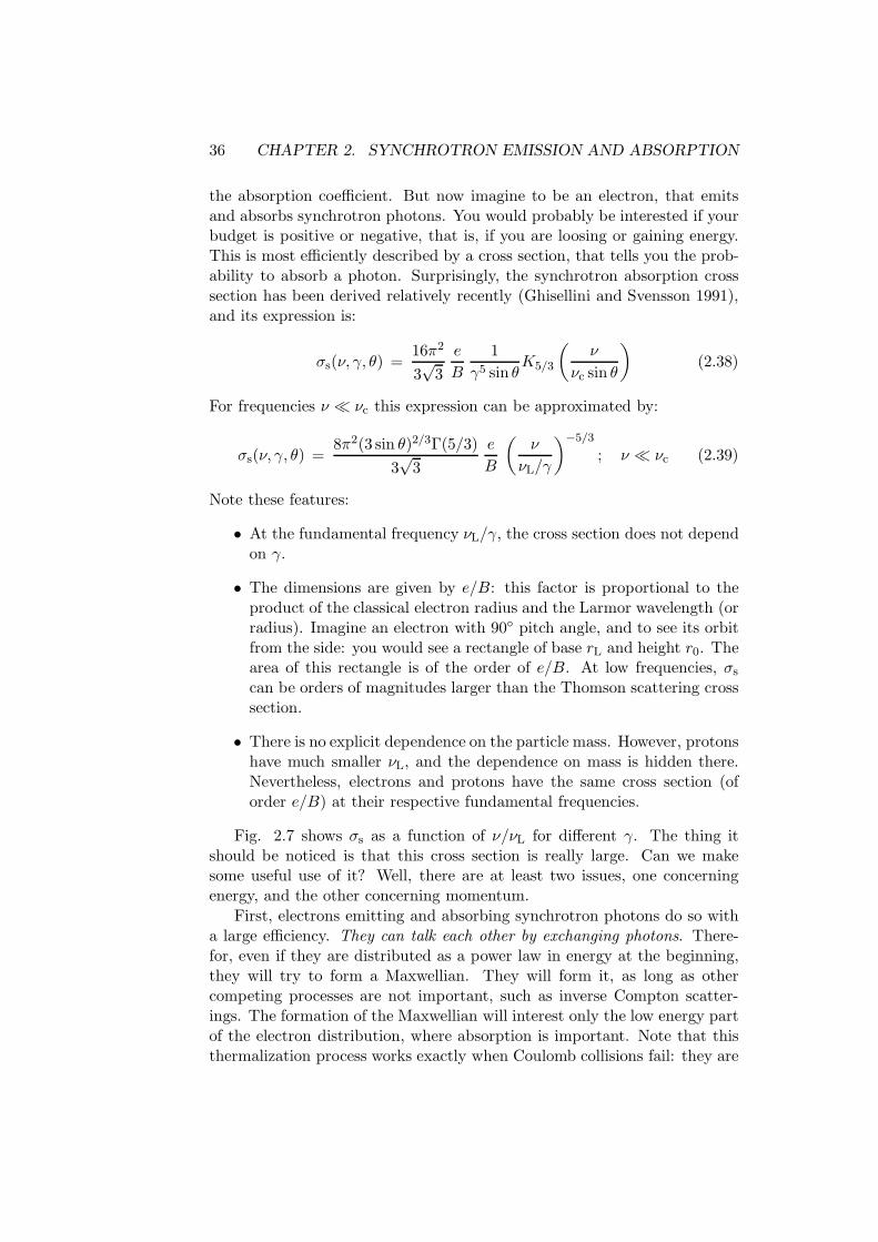
36 CHAPTER 2. SYNCHROTRON EMISSION AND ABSORPTION
the absorption coefficient. But now imagine to be an electron, that emitsand absorbs synchrotron photons. You would probably be interested if yourbudget is positive or negative, that is, if you are loosing or gaining energy.This is most efficiently described by a cross section, that tells you the prob-ability to absorb a photon. Surprisingly, the synchrotron absorption crosssection has been derived relatively recently (Ghisellini and Svensson 1991),and its expression is:
σs(ν, γ, θ) =16π2
3√
3
e
B
1
γ5 sin θK5/3
(
ν
νc sin θ
)
(2.38)
For frequencies ν ≪ νc this expression can be approximated by:
σs(ν, γ, θ) =8π2(3 sin θ)2/3Γ(5/3)
3√
3
e
B
(
ν
νL/γ
)−5/3
; ν ≪ νc (2.39)
Note these features:
• At the fundamental frequency νL/γ, the cross section does not dependon γ.
• The dimensions are given by e/B: this factor is proportional to theproduct of the classical electron radius and the Larmor wavelength (orradius). Imagine an electron with 90 pitch angle, and to see its orbitfrom the side: you would see a rectangle of base rL and height r0. Thearea of this rectangle is of the order of e/B. At low frequencies, σs
can be orders of magnitudes larger than the Thomson scattering crosssection.
• There is no explicit dependence on the particle mass. However, protonshave much smaller νL, and the dependence on mass is hidden there.Nevertheless, electrons and protons have the same cross section (oforder e/B) at their respective fundamental frequencies.
Fig. 2.7 shows σs as a function of ν/νL for different γ. The thing itshould be noticed is that this cross section is really large. Can we makesome useful use of it? Well, there are at least two issues, one concerningenergy, and the other concerning momentum.
First, electrons emitting and absorbing synchrotron photons do so witha large efficiency. They can talk each other by exchanging photons. There-for, even if they are distributed as a power law in energy at the beginning,they will try to form a Maxwellian. They will form it, as long as othercompeting processes are not important, such as inverse Compton scatter-ings. The formation of the Maxwellian will interest only the low energy partof the electron distribution, where absorption is important. Note that thisthermalization process works exactly when Coulomb collisions fail: they are

2.6. SYNCHROTRON ABSORPTION: ELECTRONS 37
inefficient at low density and high temperature, while synchrotron absorp-tion can work for relativistic electrons even if they are not very dense.
The second issue concerns exchange of momentum between photons andelectrons. Suppose that a magnetized region with relativistic electrons isilluminated by low frequency radiation by another source, located aside.The electrons will efficiently absorb this radiation, and thus its momentum.The magnetized region will then accelerate.
References
Ghisellini G. & Svensson R., 1991, MNRAS, 252, 313Ghisellini G., Haardt F. & Svensson R., 1998, MNRAS, 297, 348

38 CHAPTER 2. SYNCHROTRON EMISSION AND ABSORPTION

Chapter 3
Appendix: Useful Formulae
In this section we collect several useful formulae concerning the synchrotronemission. When possible, we give also simplified analytical expressions. Wewill often consider that the emitting electrons have a distribution in energywhich is a power law between some limits γ1 and γ2. Electrons are assumedto be isotropically distributed in the comoving frame of the emitting source.Their density is
N(γ) = Kγ−p; γ1 < γ < γ2 (3.1)
The Larmor frequency is defined as:
νL ≡ eB
2πmec(3.2)
3.1 Synchrotron
3.1.1 Emissivity
The synchrotron emissivity ǫs(ν, θ) [erg cm−3 s−1 sterad−1] is
ǫs(ν, θ) ≡ 1
4π
∫ γ2
γ1
N(γ)Ps(ν, γ, θ)dγ (3.3)
where Ps(ν, γ, θ) is the power emitted at the frequency ν (integrated overall directions) by the single electron of energy γmec
2 and pitch angle θ.For electrons making the same pitch angle θ with the magnetic field, theemissivity is
ǫs(ν, θ) =3σTcKUB
8π2νL
(
ν
νL
)− p−12
(sin θ)p+12 3
p
2
Γ(
3p−112
)
Γ(
3p+1912
)
p+ 1(3.4)
39

40 CHAPTER 3. APPENDIX: USEFUL FORMULAE
between ν1 ≫ γ21νL and ν2 ≪ γ2
2νL . If the distribution of pitch angles is
isotropic, we must average the (sin θ)p+12 term, obtaining
< (sin θ)p+12 >=
∫ π
2
0(sin θ)
p+12 sin θdθ =
√π
2
Γ(
p+54
)
Γ(
p+74
) (3.5)
Therefore the pitch angle averaged synchrotron emissivity is
ǫs(ν) =3σTcKUB
16π√πνL
(
ν
νL
)− p−12
fǫ(p) (3.6)
The function fǫ(p) includes all the products of the Γ–functions:
fǫ(p) =3
p
2
p+ 1
Γ(
3p−112
)
Γ(
3p+1912
)
Γ(
p+54
)
Γ(
p+74
)
∼ 3p
2
(
2.25
p2.2+ 0.105
)
(3.7)
where the simplified fitting function is accurate at the per cent level.
3.1.2 Absorption coefficient
The absorption coefficient κν(θ) [cm−1] is defined as:
κν(θ) ≡ 1
8πmeν2
∫ γ2
γ1
N(γ)
γ2
d
dγ
[
γ2P (ν, θ)]
dγ (3.8)
Written in this way, the above formula is valid even when the electron distri-bution is truncated. For our power law electron distribution κν(θ) becomes:
κν(θ) ≡ 1
8πmeν2
∫ γ2
γ1
N(γ)
γ2
d
dγ
[
γ2P (ν, θ)]
dγ (3.9)
Above ν = γ21νL, we have:
κν(θ) =e2K
4mec2(νL sin θ)
p+22 ν−
p+42 3
p+12 Γ
(
3p + 22
12
)
Γ
(
3p+ 2
12
)
(3.10)
Averaging over the pitch angles we have:
< (sin θ)p+22 >=
∫ π
2
0(sin θ)
p+22 sin θdθ =
√π
2
Γ(
p+64
)
Γ(
p+84
) (3.11)

3.1. SYNCHROTRON 41
resulting in a pitch angle average absorption coefficient:
κν =
√πe2K
8mecν
p+22
L ν−p+42 fκ(p) (3.12)
where the function fκ(p) is:
fκ(p) = 3p+12
Γ(
3p+2212
)
Γ(
3p+212
)
Γ(
p+64
)
Γ(
p+84
)
∼ 3p+12
(
1.8
p0.7+p2
40
)
(3.13)
The simple fitting function is accurate at the per cent level.
3.1.3 Specific intensity
Simple radiative tranfer allows to calculate the specific intensity:
I(ν) =ǫs(ν)
κν
(
1 − e−τν)
(3.14)
where the absorption optical depth τν ≡ κνR andR is the size of the emittingregion. When τν ≫ 1, the esponential term vanishes, and the intensity issimply the ratio between the emissivity and the absorption coefficient. Thisis the self–absorbed, ot thick, regime. In this case, since both ǫs(ν) andκν depends linearly upon K, the resulting self–absorbed intensity does notdepend on the normalization of the particle density K:
I(ν) =2me√3 ν
1/2L
fI(p)(
1 − e−τν)
(3.15)
we can thus see that the slope of the self–absorbed intensity does not dependon p. Its normalization, however, does (albeit weakly) depend on p throughthe function fI(p), which in the case of averaging over an isotropic pitchangle distribution is given by:
fI(p) =1
p+ 1=
Γ(
3p−112
)
Γ(
3p+1912
)
Γ(
p+54
)
Γ(
p+84
)
Γ(
3p+2212
)
Γ(
3p+212
)
Γ(
p+74
)
Γ(
p+64
)
∼ 5
4 p4/3(3.16)
where again the simple fitting function is accurate at the level of 1 per cent.

42 CHAPTER 3. APPENDIX: USEFUL FORMULAE
3.1.4 Self–absorption frequency
The self–absorption frequency νt is defined by τνt = 1:
νt = νL
[√πe2RK
8mecνLfκ(p)
]
4p+4
= νL
[
π√π
4
eRK
Bfκ(p)
]2
p+4
(3.17)
Note that the term in parenthesis is adimensional, and since RK has unitsof the inverse of a surface, then e/B has the dimension of a surface. Infact we have already discussed that this is the synchrotron absorption crosssection of a relativistic electron of energy γmec
2 absorbing photons at thefundamental frequency νL/γ.
The random Lorentz factor γt of the electrons absorbing (and emitting)photons with frequency νt is γt ∼ [3νt/(4νL)]1/2.
3.1.5 Synchrotron peak
In a F (ν) plot, the synchrotron spectrum peaks close to νt, at a frequencyνs,p given by solving
dI(ν)
dν= 0 → d
dν
[
ν5/2(
1 − e−τν)
]
= 0 (3.18)
which is equivalent to solve the equation:
exp(
τνs,p
)
− p+ 4
5τνs,p
− 1 = 0 (3.19)
whose solution can be approximated by
τνs,p∼ 2
5p1/3 ln p (3.20)

Chapter 4
Compton scattering
4.1 Introduction
The simplest interaction between photons and free electrons is scattering.When the energy of the incoming photons (as seen in the comoving frameof the electron) is small with respect to the electron rest mass–energy, theprocess is called Thomson scattering, which can be described in terms ofclassical electro–dynamics. As the energy of the incoming photons increasesand becomes comparable or greater than mec
2, a quantum treatment isnecessary (Klein–Nishina regime).
4.2 The Thomson cross section
Assume an electron at rest, and an electromagnetic wave of frequency ν ≪mec
2/h. Assume also that the incoming wave is completely linearly po-larized. In order to neglect the magnetic force (e/c)(v ×B) we must alsorequire that the oscillation velocity v ≪ c. This in turn implies that theincoming wave has a sufficiently low amplitude. The electron start to os-cillate in response to the varying electric force eE, and the average squareacceleration during one cicle of duration T = 1/ν is
〈a2〉 =1
T
∫ T
0
e2E20
m2e
sin2(2πνt) dt =e2E2
0
2m2e
(4.1)
The emitted power per unit solid angle is given by the Larmor formuladP/dΩ = e2a2 sin2 Θ/(4πc3) where Θ is the angle between the accelerationvector and the propagation vector of the emitted radiation. Please notethat Θ is not the scattering angle, which is instead the angle between theincoming and the scattered wave (or photon). We then have
dPe
dΩ=
e4E20
8πm2ec
3sin2 Θ (4.2)
43

44 CHAPTER 4. COMPTON SCATTERING
The scattered radiation is completely linearly polarized in the plane definedby the incident polarization vector and the scattering direction. The flux ofthe incoming wave is Si = cE2
0/(8π). The differential cross section of theprocess is then
(
dσ
dΩ
)
pol
=dPe/dΩ
Si= r20 sin2 Θ (4.3)
where r0 ≡ e2/(mec2) is the classic electron radius, r0 = 2.82×10⁻¹³ cm. We
see that the scattered pattern of a completely polarized incoming wave is atorus, with axis along the acceleration direction. The total cross section canbe derived in a similar way, but considering the Larmor formula integratedover the solid angle [P = 2e2a2/(3c3)]. In this way the total cross section is
σpol =Pe
Si=
8π
3r20 (4.4)
Note that the classical electron radius can also be derived by equating theenergy of the associated electric field to the electron rest mass–energy:
mec2 =
∫ ∞
ao
E2
8π4πr2dr =
∫ ∞
ao
e2
2r2dr → a0 =
1
2
e2
mec2(4.5)
Why is a0 slightly different from r0? Because there is an intrinsic uncertaintyrelated to the distribution of the charge within (or throughout the surfaceof) the electron. See the discussion in Vol. 2, chapter 28.3 of “The FeynmanLectures on Physics”, about the fascinating idea that the mass of the electronis all electromagnetic.
4.2.1 Why the peanut shape?
The scattering of a completely unpolarized incoming wave can be derivedby assuming that the incoming radiation is the sum of two orthogonal com-pletely linearly polarized waves, and then summing the associated scatteringpatterns. Since we have the freedom to chose the orientations of the twopolarization planes, it is convenient to chose one of these planes as the onedefined by the incident and scattered directions, and the other one perpen-dicular to this plane. The scattering can be then regarded as the sum oftwo independent scattering processes, one with emission angle Θ, the otherwith π/2. If we note that the scattering angle (i.e. the angle between thescattered wave and the incident wave) is θ = π/2 − Θ, we have
(
dσ
dΩ
)
unpol
=1
2
[
(
dσ(Θ)
dΩ
)
pol
+
(
dσ(π/2)
dΩ
)
pol
]
=1
2r20(1 + sin2 Θ)
=1
2r20(1 + cos2 θ) (4.6)
4.2. THE THOMSON CROSS SECTION 45
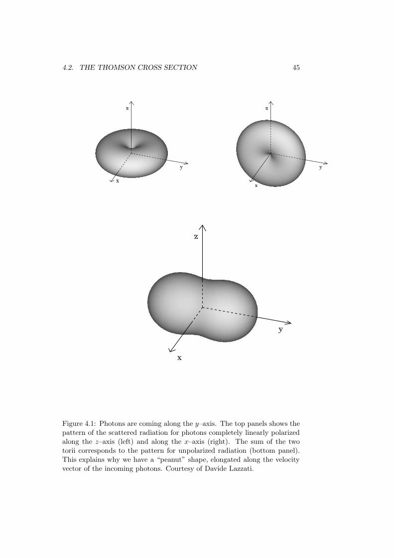
Figure 4.1: Photons are coming along the y–axis. The top panels shows thepattern of the scattered radiation for photons completely linearly polarizedalong the z–axis (left) and along the x–axis (right). The sum of the twotorii corresponds to the pattern for unpolarized radiation (bottom panel).This explains why we have a “peanut” shape, elongated along the velocityvector of the incoming photons. Courtesy of Davide Lazzati.

46 CHAPTER 4. COMPTON SCATTERING
In this case we see that the cross section depends only on the scatteringangle θ. The pattern of the scattered radiation is then the superpositionof two orthogonal “tori” (one for each polarization direction), as illustratedin Fig. 4.1. When scattering completely linearly polarized radiation, onlyone “torus” survives. Instead, when scattering unpolarized radiation, somepolarization is introduced, because of the difference between the two “tori”patterns. Both terms of the RHS of Eq. 4.6 refer to completely polarizedscattered waves (but in two perpendicular planes). The difference betweenthese two terms is then associated to the introduced polarization, which isthen
Π =1 − cos2 θ
1 + cos2 θ(4.7)
The above discussion help to understand why the scattering process intro-duces some polarization, which is maximum (100%) if the angle between theincoming and the scattered photons is 90 (only one torus contributes), andzero for 0 and 180, where the two torii give the same contribution.
The total cross section, integrated over the solid angle, is the same asthat for polarized incident radiation (Eq. 4.4) since the electron at rest hasno preferred defined direction. This is the Thomson cross section:
σT =
∫(
dσ
dΩ
)
unpol
dΩ =2πr20
2
∫
(1 + cos2 θ)d cos θ =8π
3r20
= 6.65 × 10⁻²⁵ cm2 (4.8)
4.3 Direct Compton scattering
In the previous section we considered the scattering process as an interactionbetween an electron and an electromagnetic wave. This required hν ≪mec
2. In the general case the quantum nature of the radiation must betaken into account. We consider then the scattering process as a collisionbetween the electron and the photon, and apply the conservation of energyand momentum to derive the energy of the scattered photon. It is convenientto measure energies in units of mec
2 and momenta in units of mec.Consider an electron at rest and an incoming photon of energy x0, which
becomes x1 after scattering. Let θ be the angle between the incoming andoutgoing photon directions. This defines the scattering plane. Momentumconservation dictates that also the momentum vector of the electron, afterthe scattering, lies in the same plane. Conservation of energy and conserva-tion of momentum along the x and y axis gives:
x1 =x0
1 + x0(1 − cos θ)(4.9)
Note that, for x0 ≫ 1 and cos θ 6= 1, x1 → (1 − cos θ)−1. In this case thescattered photon carries information about the scattering angle, rather than

4.4. THE KLEIN–NISHINA CROSS SECTION 47
about the initial energy. As an example, for θ = π and x0 ≫ 1, the finalenergy is x1 = 0.5 (corresponding to 255 keV) independently of the exactvalue of the initial photon energy. Note that for x0 ≪ 1 the scattered energyx1 ≃ x0, as assumed in the classical Thomson scattering. The energy shiftimplied by Eq. 4.9 is due to the recoil of the electron originally at rest, andbecomes significant only when x0 becomes comparable with 1 (or more).When the energy of the incoming photon is comparable to the electron restmass, another quantum effect appears, namely the energy dependence of thecross section.
4.4 The Klein–Nishina cross section
The Thomson cross section is the classical limit of the more general Klein–Nishina cross section (here we use x as the initial photon energy, instead ofx0, for simplicity):
dσKN
dΩ=
3
16πσT
(x1
x
)2(
x
x1+x1
x− sin2 θ
)
(4.10)
This is a compact form, but there appears dependent quantities, as sin θ isrelated to x and x1. By inserting Eq. 4.9, we arrive to
dσKN
dΩ=
3
16π
σT
[1 + x(1 − cos θ)]2
[
x(1 − cos θ) +1
1 + x(1 − cos θ)+ cos2 θ
]
(4.11)In this form, only independent quantities appear (i.e. there is no x1). Notethat the cross section becomes smaller for increasing x and that it coincideswith dσT/dΩ for θ = 0 (for this angle x1 = x independently of x). Thishowever corresponds to a vanishingly small number of interactions, sincedΩ → 0 for θ → 0).
Integrating Eq. 4.11 over the solid angle, we obtain the total Klein–Nishina cross section:
σKN =3
4σT
1 + x
x3
[
2x(1 + x)
1 + 2x− ln(1 + 2x)
]
+1
2xln(1 + 2x) − 1 + 3x
(1 + 2x)2
(4.12)
Asimptotic limits are:
σKN ≃ σT
(
1 − 2x+26x2
5+ ...
)
; x≪ 1
σKN ≃ 3
8
σT
x
[
ln(2x) +1
2
]
; x≫ 1 (4.13)
The direct Compton process implies a transfer of energy from the photons tothe electrons. It can then be thought as an heating mechanism. In the next

48 CHAPTER 4. COMPTON SCATTERING
Figure 4.2: The total Klein–Nishina cross section as a function of energy.The dashed line is the approximation at high energies as given in Eq. 4.13.
Figure 4.3: The differential Klein–Nishina cross section (in units of σT),for different incoming photon energies. Note how the scattering becomespreferentially forward as the energy of the photon increases.

4.4. THE KLEIN–NISHINA CROSS SECTION 49
Figure 4.4: Scattered photons energies as a function of the scattering angle,for different incoming photon energies. Note that, for x ≫ 1 and for largescattering angle, the scattered photon energies becomes x1 ∼ 1/2, indepen-dent of the initial photon energy x.
subsection we discuss the opposite process, called inverse Compton scatter-
ing, in which hot electrons can transfer energy to low frequency photons.We have so far neglected the momentum exchange between radiation
and the electron. One can see, even classically, that there must be a netforce acting along the direction of the wave if one considers the action ofthe magnetic field of the wave. In fact the Lorentz force ev × B is always
directed along the direction of the wave (here v is the velocity along the E
field). This explains the fact that light can exert a pressure, even classically.
4.4.1 Another limit
We have mentioned that, in order for the magnetic Lorentz force to be neg-ligible, the electron must have a transverse (perpendicular to the incomingwave direction) velocity ≪ c. Considering a wave of frequency ω and electricfield E = E0 sin(ωt), this implies that:
v⊥c
=
∫ T/2
0
eE0
cmesin(ωt)dt =
2eE0
mecω≪ 1 (4.14)
This means that the scattering process can be described by the Thomsoncross section if the wave have a sufficiently low amplitude and a not toosmall frequency (i.e. for very small frequencies the electric field of the waveaccelerates the electron for a long time, and then to large velocities).

50 CHAPTER 4. COMPTON SCATTERING
4.4.2 Pause
Now pause, and ask if there are some ways to apply what we have done upto now to real astrophysical objects.
• The Eddington luminosity is derived with the Thomson cross section,with the thought that it describes the smallest probability of inter-action between matter and radiation. But the Klein–Nishina crosssection can be even smaller, as long as the source of radiation emitsat high energy. What are the consequences? If you have forgotten thedefinition of the Eddington luminosity, here it is:
LEdd =4πGMmp
σT= 1.5 × 1038 M
M⊙erg s−1 (4.15)
• In Nova Muscae, some years ago a (transient) annihilation line wasdetected, together with another feature (line–like) at 200 keV. Whatcan this feature be?
• It seems that high energy radiation can suffer less scattering and there-fore can propagate more freely through the universe. Is that true? Canyou think to other processes that can kill high energy photons in space?
• Suppose to have an astrophysical source of radiation very powerfulabove say – 100 MeV. Assume that at some distance there is a veryefficient “reflector” (i.e. free electrons) and that you can see the scat-tered radiation. Can you guess the spectrum you receive? Does itcontain some sort of “pile–up” or not? Will this depend upon thescattering angle?
4.5 Inverse Compton scattering
When the electron is not at rest, but has an energy greater that the typicalphoton energy, there can be a transfer of energy from the electron to thephoton. This process is called inverse Compton to distinguish it from thedirect Compton scattering, in which the electron is at rest, and it is thephoton to give part of its energy to the electron.
We have two regimes, that are called the Thomson and the Klein–Nishina
regimes. The difference between them is the following: we go in the framewhere the electron is at rest, and in that frame we calculate the energy of theincoming photon. If the latter is smaller than mec
2 we are in the Thomsonregime. In this case the recoil of the electron, even if it always exists, issmall, and can be neglected. In the opposite case (photon energies largerthan mec
2), we are in the Klein–Nishina one, and we cannot neglect therecoil. As we shall see, in both regimes the typical photon gain energy, even

4.5. INVERSE COMPTON SCATTERING 51
if there will always be some arrangements of angles for which the scatteredphoton looses part of its energy.
4.5.1 Thomson regime
Perhaps, a better name should be “inverse Thomson” scattering, as willappear clear shortly.
4.5.2 Typical frequencies
In the frame K ′ comoving with the electron, the incoming photon energy is
x′ = xγ(1 − β cosψ) (4.16)
where ψ is the angle between the electron velocity and the photon direction(see Fig 4.5). Then if x′ ≪ 1, we are in the Thomson regime. In the restframe of the electron the scattered photon will have the same energy x′1 asbefore the scattering, independent of the scattering angle. Then
x′1 = x′ (4.17)
This photon will be scattered at an angle ψ′1 with respect to the electron
Figure 4.5: In the lab frame an electron is moving with velocity v. Itsvelocity makes an angle ψ with an incoming photon of frequency ν. In theframe where the electron is at rest, the photon is coming from the front,with frequency ν ′, making an angle ψ′ with the direction of the velocity.
52 CHAPTER 4. COMPTON SCATTERING
velocity. Going back to K the observer sees
x1 = x′1γ(1 + β cosψ′1) (4.18)
Recalling Eq. 1.15, for the transformation of angles:
cosψ′1 =
β + cosψ1
1 + β cosψ1(4.19)
we arrive to the final formula:
x1 = x1 − β cosψ
1 − β cosψ1(4.20)
Now all quantities are calculated in the lab–frame.
Figure 4.6: Minimum and maximum scattered frequencies. The maximumoccurs for head-on collisions, the minimum for tail–on ones. These twofrequencies are one the inverse of the other.
Let us see the minimum and maximum energies. The maximum is whenψ = π (head on collision), and when ψ1 = 0 (the photon is scattered alongthe electron velocity vector). In these are head–on collisions:
x1 = x1 + β
1 − β= γ2(1 + β)2x → 4γ2x; head − on (4.21)
where the last step is valid if γ ≫ 1. The other extreme is for ψ1 = π andψ = 0. In this case the incoming photon “comes from behind” and bouncesback. In these “tail–on” collisions:
x1 = x1 − β
1 + β=
x
γ2(1 + β)2→ x
4γ2; tail − on (4.22)

4.5. INVERSE COMPTON SCATTERING 53
where again the last step is valid if γ ≫ 1. Another typical angle is sinψ1 =1/γ, corresponding to cosψ1 = β. This corresponds to the aperture angleof the beaming cone. For this angle:
x1 =1 − β cosψ
1 − β2x = γ2(1 − β cosψ)x; beaming cone (4.23)
which becomes x1 = x/(1 + β) for ψ = 0, x1 = γ2x for ψ = π/2 andx1 = γ2(1 + β)x for ψ = π.
For an isotropic distribution of incident photons and for γ ≫ 1 theaverage photon energy after scattering is (see Eq. 4.45):
〈x1〉 =4
3γ2x (4.24)
Total loss rate
We can simply calculate the rate of scatterings per electron considering allquantities in the lab–frame. Let n(ǫ) be the density of photons of energyǫ = hν, v the electron velocity and ψ the angle between the electron velocityand the incoming photon. For mono–directional photon distributions, wehave:
dN
dt=
∫
σTvreln(ǫ)dǫ (4.25)
vrel = c−v cosψ is the relative velocity between the electron and the incom-ing photons. We then have
dN
dt=
∫
σTc(1 − β cosψ)n(ǫ)dǫ (4.26)
Note that the rate of scatterings in the lab frame, when the electron and/orphoton are anisotropically distributed, can be described by an effective crosssection σeff ≡
∫
σT(1 − β cosψ)dΩ/4π. For photons and electrons movingin the same direction the scattering rate (hence, the effective optical depth)can be greatly reduced.
The power contained in the scattered radiation is then
dEγ
dt=
ǫ1dN
dt= σTc
∫
(1 − β cosψ)2
1 − β cosψ1ǫn(ǫ)dǫ (4.27)
Independently of the incoming photon angular distribution, the averagevalue of 1 − β cosψ1 can be calculated recalling that, in the rest frame ofthe electron, the scattering has a backward–forward symmetry, and there-fore 〈cosψ′
1〉 = π/2. The average value of cosψ1 is then β, leading to〈1 − β cosψ1〉 = 1/γ2. We therefore obtain
dEγ
dt= σTcγ
2
∫
(1 − β cosψ)2ǫn(ǫ)dǫ (4.28)

54 CHAPTER 4. COMPTON SCATTERING
If the incoming photons are isotropically distributed, we can average out(1−β cosψ)2 over the solid angle, obtaining 1 +β2/3. The power producedis then
dEγ
dt= σTcγ
2
(
1 +β2
3
)
Ur (4.29)
where
Ur =
∫
ǫn(ǫ)dǫ (4.30)
is the energy density of the radiation before scattering. This is the powercontained in the scattered radiation. To calculate the energy loss rate of theelectron, we have to subtract the initial power of the radiation eventuallyscattered
Pc(γ) ≡ dEe
dt=
dEγ
dt− σTcUr =
4
3σTcγ
2β2Ur (4.31)
A simple way to remember Eq. 4.31 is:
Pc(γ) =
(
# of collisions
sec
)
(average phot. energy after scatt.)
=
(
σTcUr
〈hν〉
) (
4
3〈hν〉γ2
)
(4.32)
Note the similarity with the synchrotron energy loss. The two energy lossrates are identical, once the radiation energy density is replaced by themagnetic energy density UB. Therefore, if relativistic electrons are in aregion with some radiation and magnetic energy densities, they will emit byboth the synchrotron and the Inverse Compton scattering processes. Theratio of the two luminosities will be
Lsyn
LIC=
Psyn
Pc=
UB
Ur(4.33)
where we have set dEIC/dt = dEe/dt. This is true unless one of the twoprocesses is inhibited for some reason. For instance:
• At (relatively) low energies, electrons could emit and absorb synchrotronradiation, so the synchrotron cooling is compensated by the heatingdue to the absorption process.
• At high energies, electrons could scatter in the Klein–Nishina regime:in this case, since the cross section is smaller, they will do less scat-terings, and cool less.
But let us go back to Eq. 4.28, that is the starting point when dealingwith anisotropic seed photon distributions. Think for instance to an accre-tion disk as the producer of the seed photons for scattering, and some cloudof relativistic electrons above the disk. If the cloud is not that distant, and

4.5. INVERSE COMPTON SCATTERING 55
Figure 4.7: In the center of a semi–sphere (the “bowl”) we have relativisticelectrons going down and going up, all with the same γ. Since the seedphoton distribution is anisotropic, so is the scattered radiation and power.The losses of the electron going down are 7 times larger than those of theelectron going up (if γ ≫ 1). Since almost all the radiation is producedalong the velocity vector of the electrons, also the downward radiation is 7times more powerful than the upward radiation.
it is small with respect to the disk size, then this case is completely equal tothe case of having a little cloud of relativistic electrons located at the centerof a semi–sphere. That is, we have the “bowl” case illustrated in Fig 4.7.Just for fun, let us calculate the total power emitted by an electron going“up” and by its brother (i.e. it has the same γ) going down. Using Eq. 4.28we have:
Pdown
Pup=
∫ 0−1(1 − βµ)2dµ
∫ −10 (1 − βµ)2dµ
=1 + β + β2/3
1 − β + β2/3→ 7 (4.34)
where µ ≡ cosψ and the last step assumes β → 1. Since almost all theradiation is produced along the velocity vector of the electrons, also thedownward radiation is more powerful than the upward radiation (i.e. 7times more powerful for γ ≫ 1). What happens if the cloud of electronsis located at some height above the bowl? Will the Pdown/Pup be more orless?

56 CHAPTER 4. COMPTON SCATTERING
4.5.3 Cooling time and compactness
The cooling time due to the inverse Compton process is
tIC =E
dEe/dt=
3γmec2
4σTcγ2β2Ur∼ 3mec
2
4σTcγUr; γǫ≪ mec
2 (4.35)
This equation offers the opportunity to introduce an important quantity,namely the compactness of an astrophysical source, that is essentially theluminosity L over the size R ratio. Consider in fact how Ur and L are related:
Ur =L
4πR2c(4.36)
Although this relation is almost universally used, there are subtleties. Itis surely valid if we measured Ur outside the source, at a distance R fromits center. In this case 4πR2c is simply the volume of the shell crossed bythe source radiation in one second. But if we are inside an homogeneous,spherical transparent source, a better way to calculate Ur is to think tothe average time needed to the typical photon to exit the source. This istesc = 3R/(4c). It is less than R/c because the typical photon is not bornat the center (there is more volume close to the surface). If V = (4π/3)R3
is the volume, we can write:
Ur =L
Vtesc =
3L
4πR3
3R
4c=
9L
16πR2c(4.37)
This is greater than Eq. 4.36 by a factor 9/4. Anyway, let us be conventionaland insert Eq. 4.36 in Eq. 4.35:
tIC =3πmec
2R2
σTγL→ tIC
R/c=
3π
γ
mec3R
σTL≡ 3π
γ
1
ℓ(4.38)
where the dimensionless compactness ℓ is defined as
ℓ =σTL
mec3R(4.39)
For ℓ close or larger than unity, we have that even low energy electrons coolby the Inverse Compton process in less than a light crossing time R/c.
There is another reason why ℓ is important, related to the fact thatit directly measures the optical depth (hence the probability to occur) ofthe photon–photon collisions that lead to the creation of electron–positronpairs. The compactness is one of the most important physical parameterswhen studying compact high energy compact sources (X–ray binaries, AGNsand Gamma Ray Bursts).

4.5. INVERSE COMPTON SCATTERING 57
4.5.4 Single particle spectrum
As we did for the synchrotron spectrum, we will not repeat the exact deriva-tion of the single particle spectrum, but we try to explain why the typicalfrequency of the scattered photon is a factor γ2 larger than the frequency ofthe incoming photon. Here are the steps to consider:
1. Assume that the relativistic electron travels in a region where thereis a radiation energy density Ur made by photons which we will take,for simplicity, monochromatic, therefore all having a dimensionlessfrequency x = hν/mec
2.
2. In the frame where the electron is at rest, half of the photon appearto come from the front, within an angle 1/γ.
3. The typical frequency of these photon is x′ ∼ γx (it is twice that forphotons coming exactly head on).
4. Assuming that we are in the Thomson regime means that i) x′ < 1; ii)the cross section is the Thomson one; iii) the frequency of the scatteredphoton is the same of the incoming one, i.e. x′1 = x′ ∼ γx, and iv)the pattern of the scattered photons follows the angular dependenceof the cross section, therefore the “peanut”.
5. Independently of the initial photon direction, and therefore indepen-dently of the frequencies seen by the electrons, all photons after scat-terings are isotropized. This means that all observer (at any angle ψ′
1
in this frame see the same spectrum, and the same typical frequency.Half of the photons are in the semi-sphere with ψ′
1 ≤ π/2.
6. Now we go back to the lab–frame. Those photons that had ψ′1 ≤ π/2
now have ψ1 ≤ 1/γ. Their typical frequency if another factor γ greaterthan what they had in the rest frame, therefore
x1 ∼ γ2x (4.40)
This is the typical Inverse Compton frequency.
The exact derivation can be found e.g. in Rybicki & Lightman (1979)and in Blumenthal & Gould (1970). We report here the final result, validfor a monochromatic and isotropic seed photons distribution, characterizedby a specific intensity
I(x)
x=
I0xδ(x− x0) (4.41)
Note that I(x)/x is the analog of the normal intensity, but it is associatedwith the number of photons. If we have n electrons per cubic centimeter wehave:
ǫIC(x1) =σTnI0(1 + β)
4γ2β2x0FIC(x1) (4.42)
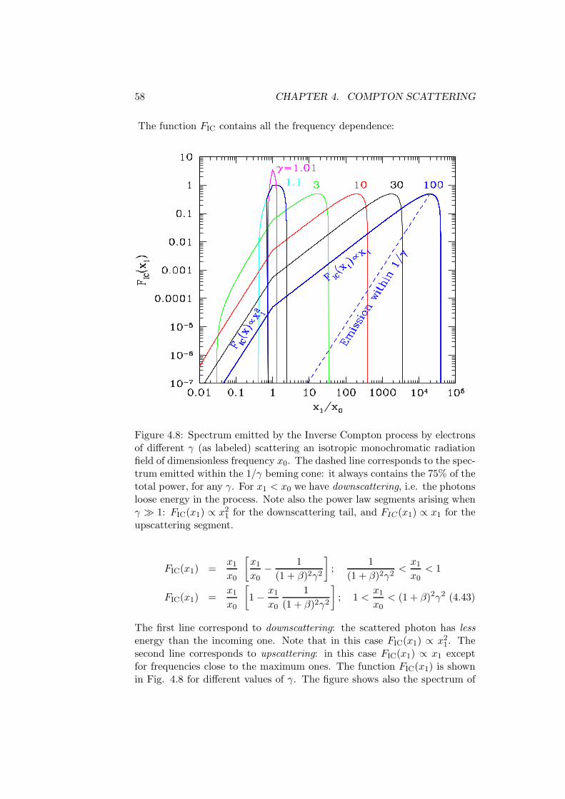
58 CHAPTER 4. COMPTON SCATTERING
The function FIC contains all the frequency dependence:
Figure 4.8: Spectrum emitted by the Inverse Compton process by electronsof different γ (as labeled) scattering an isotropic monochromatic radiationfield of dimensionless frequency x0. The dashed line corresponds to the spec-trum emitted within the 1/γ beming cone: it always contains the 75% of thetotal power, for any γ. For x1 < x0 we have downscattering, i.e. the photonsloose energy in the process. Note also the power law segments arising whenγ ≫ 1: FIC(x1) ∝ x2
1 for the downscattering tail, and FIC(x1) ∝ x1 for theupscattering segment.
FIC(x1) =x1
x0
[
x1
x0− 1
(1 + β)2γ2
]
;1
(1 + β)2γ2<x1
x0< 1
FIC(x1) =x1
x0
[
1 − x1
x0
1
(1 + β)2γ2
]
; 1 <x1
x0< (1 + β)2γ2 (4.43)
The first line correspond to downscattering: the scattered photon has less
energy than the incoming one. Note that in this case FIC(x1) ∝ x21. The
second line corresponds to upscattering: in this case FIC(x1) ∝ x1 exceptfor frequencies close to the maximum ones. The function FIC(x1) is shownin Fig. 4.8 for different values of γ. The figure shows also the spectrum of

4.6. EMISSION FROM MANY ELECTRONS 59
the photons contained in the beaming cone 1/γ: the corresponding power isalways 75% of the total.
The average frequency of FIC(x1) is
〈x1〉 = 2γ2x0; energy spectrum (4.44)
This is the average frequency of the energy spectrum. We sometimes wantto know the average energy of the photons, i.e. we have to calculate theaverage frequency of the photon spectrum FIC(x1)/x1. This is:
〈x1〉 =4
3γ2x0; photon spectrum (4.45)
4.6 Emission from many electrons
We have seen that the emission spectrum from a single particle is peaked,and the typical frequency is boosted by a factor γ2. This is equal to thesynchrotron case. Therefore we can derive the Inverse Compton emissiv-ity as we did for the synchrotron one. Again, assume a power–law energydistribution for the relativistic electrons:
N(γ) = Kγ−p = N(E)dE
dγ; γmin < γ < γmax (4.46)
and assume that it describes an isotropic distribution of electrons. Forsimplicity, let us assume that the seed photons are isotropic and monochro-matic, with frequency ν0 (we now pass to real frequencies, since we aregetting closer to the real world..). Since there is a strong link between thescattered frequency νc and the electron energy that produced it, we can set:
νc =4
3γ2ν0 → γ =
(
3νc
4ν0
)1/2
→∣
∣
∣
∣
dγ
dν
∣
∣
∣
∣
=ν−1/2c
2
(
3
4νo
)1/2
(4.47)
Now, repeating the argument we used for synchrotron emission, we can statethat the power lost by the electron of energy γmec
2 within mec2dγ goes into
the radiation of frequency ν within dν. Since we will derive an emissivity(i.e. erg cm−3 s−1 sterad−1 Hz−1) we must remember the 4π term (if theemission is isotropic). We can set:
ǫc(νc)dνc =1
4πmec
2Pc(γ)N(γ)dγ (4.48)
This leads to:
ǫc(νc) =1
4π
(4/3)α
2σTcK
Ur
ν0
(
νc
ν0
)−α
(4.49)
Again, a power law, as in the case of synchrotron emission by a power lawenergy distribution. Again the same link between α and p:
α =p− 1
2(4.50)

60 CHAPTER 4. COMPTON SCATTERING
Of course, this is not a coincidence: it is because both the Inverse Comptonand the synchrotron single electron spectra are peaked at a typical frequencythat is a factor γ2 greater than the starting one.
Eq. 4.49 becomes a little more clear if
• we express ǫc(νc) as a function of the photon energy hνc. Thereforeǫc(hνc) = ǫc(νc)/h;
• we multiply and divide by the source radius R;
• we consider a proxy for the scattering optical depth of the relativisticelectrons setting τc ≡ σTKR.
Then we obtain:
ǫc(hνc) =1
4π
(4/3)α
2
τcR/c
Ur
hν0
(
νc
ν0
)−α
(4.51)
In this way: τc (for τc < 1) is the fraction of the seed photons Ur/hν0
undergoing scattering in a time R/c, and νc/ν0 ∼ γ2 is the average gain inenergy of the scattered photons.
4.6.1 Non monochromatic seed photons
It is time to consider the more realistic case in which the seed photons arenot monochromatic, but are distributed in frequency. This means that wehave to integrate Eq. 4.49 over the incoming photon frequencies. For clarity,let us drop the subscript 0 in ν0. We have
ǫc(νc) =1
4π
(4/3)α
2
τcR/c
ν−αc
∫ νmax
νmin
Ur(ν)
νναdν (4.52)
where Ur(ν) [erg cm−3 Hz−1] is the specific radiation energy density atthe frequency ν. The only difficulty of this integral is to find the correctlimit of the integration, that, in general, depend on νc. Note also anotherinteresting thing. We have just derived that if the same electron populationproduces Inverse Compton and synchrotron emission, than the slopes of thetwo spectra are the same. Therefore, when Ur(ν) is made by synchrotronphotons, then Ur(ν) ∝ ν−α. The result of the integral, in this case, will beln(νmax/νmin).
Fig. 4.9 helps to understand what are the right νmax and νmin to use.On the y–axis we have the frequencies of the seed photon distribution, whichextend between ν1 and ν2. On the x–axis we have the scattered frequencies,which extend between νc,1 = (4/3)γ2
minν1 and νc,4 = (4/3)γ2maxν1. The
diagonal lines are the functions
ν =3νc
4γ2min
ν =3νc
4γ2max
(4.53)

4.6. EMISSION FROM MANY ELECTRONS 61
Figure 4.9: The ν–νc plane. The two diagonal lines delimit the regions ofthe seed photons that can be used to give a given frequency νc.
that tell us what are the appropriate ν that can give νc once we change γ.There are three zones:
1. In zone (1), between νc,1 and νc,2 = (4/3)γ2minν2 the appropriate limits
of integration are:
νmin = ν1 νmax =3νc
4γ2min
(4.54)
2. In zone (2), between νc,2 and νc,3 = (4/3)γ2maxν1 the limits are:
νmin = ν1 νmax = ν2 (4.55)
3. In zone (3), between νc,3 and νc,4 = (4/3)γ2maxν2 the limits are:
νmin =3νc
4γ2max
νmax = ν2 (4.56)
We see that only in zone (2) the limits of integration coincide with the exten-sion in frequency of the seed photon distribution, and are therefore constant.Therefore ǫc(νc) will be a power law of slope α only in the correspondingfrequency limits. Note also that for a narrow range [ν1; ν2] or a narrow rangein [γmin; γmax] we do not have a power law, since there is no νc for which thelimits of integrations are both constant.

62 CHAPTER 4. COMPTON SCATTERING
4.7 Thermal Comptonization
With this term we mean the process of multiple scattering of a photon dueto a thermal or quasi–thermal distribution of electrons. By quasi–thermal
we mean a particle distribution that is peaked, even if it is not a perfectMaxwellian. Since the resulting spectrum, by definition, is due to the su-perposition of many spectra, each corresponding to a single scattering, thedetails of the particle distribution will be lost in the final spectrum, as longas the distribution is peaked. The “bible” for an extensive discussion aboutthis process is Pozdnyakov, Sobol & Sunyaev (1983).
There is one fundamental parameter measuring the importance of theInverse Compton process in general, and of multiple scatterings in partic-ular: the Comptonization parameter, usually denoted with the letter y. Itsdefinition is:
y = [average # of scatt.] × [average fractional energy gain for scatt.](4.57)
If y > 1 the Comptonization process is important, because the Comptonizedspectrum has more energy than the spectrum of the seed photons.
4.7.1 Average number of scatterings
This can be calculated thinking that the photon, before leaving the source,experience a sort of random walk inside the source. Let us call
τT = σTnR (4.58)
the Thomson scattering optical depth, where n is the electron density andR the size of the source. When τT < 1 most of the photons leave the sourcedirectly, without any scattering. When τT > 1 then the mean free path isd = R/τT and the photon will experience, on average, τ2
T scatterings beforeleaving the source. Therefore the total path travel by the photon, from thetime of its birth to the time it leaves the source is: the photon is born, is
c∆t = τ2T
R
τT= τTR (4.59)
and ∆t is the corresponding elapsed time.
4.7.2 Average gain per scattering
Relativistic case
If the scattering electrons are relativistic, we have already seen that thephoton energy is amplified by the factor (4/3)γ2 (on average). Therefore

4.7. THERMAL COMPTONIZATION 63
the problem is to find what is 〈γ2〉 in the case of a relativistic Maxwellian,that has the form
N(γ) ∝ γ2e−γ/Θ; Θ ≡ kT
mec2(4.60)
Setting x0 = hν0/(mec2) we have that the average energy of the photon of
initial frequency x0 after a single scattering with electron belonging to thisMaxwellian is:
〈x1〉 =4
3〈γ2〉 =
4
3x0
∫ ∞1 γ2γ2e−γ/Θdγ∫ ∞1 γ2e−γ/Θdγ
=4
3x0Θ
2 Γ(5)
Γ(3)
=4
3x0
4!
2!= 16Θ2x0 (4.61)
Non relativistic case
In this case the average gain is proportional to the electron energy, notto its square. The derivation is not immediate, but we must use a trick.Also, we have to account that in any Maxwellian, but especially when thetemperature is not large, there will be electrons that have less energy thanthe incoming photons. In this case it is the photon to give energy to theelectron: correspondingly, the scattered photon will have less energy thanthe incoming one. Averaging out over a Maxwellian distribution, we willhave:
∆x
x=
x1 − x0
x0= αΘ − x (4.62)
Where αΘ is what the photon gains and the −x term corresponds to thedownscattering of the photon (i.e. direct Compton). We do not know yetthe value for the constant α. To determine it we use the following argument.We know (from general and robust arguments) what happens when photonsand electrons are in equilibrium under the only process of scattering, andneglecting absorption (i.e. when the number of photon is conserved). Whathappens is that the photons follow the so–called Wien distribution given by:
FW(x) ∝ x3e−x/Θ → NW(x) =FW(x)
x∝ x2e−x/Θ (4.63)
where F correspond to the radiation spectrum, N to the photon spectrum,and Θ is the dimensionless electron temperature. When a Wien distributionis established we must have 〈∆x〉 = 0, since we are at equilibrium, So werequire that, on average, gains equal losses:
〈∆x〉 = 0 → αΘ〈x〉 − 〈x2〉 = 0 (4.64)

64 CHAPTER 4. COMPTON SCATTERING
Calculating 〈x〉 and 〈x2〉 for a photon Wien distribution, we have:
〈x〉 =
∫ ∞0 x3e−x/Θdx
∫ ∞0 x2e−x/Θdx
=Γ(4)
Γ(3)Θ =
3!
2!Θ = 3Θ
〈x2〉 =
∫ ∞0 x4e−x/Θdx
∫ ∞0 x3e−x/Θdx
=Γ(5)
Γ(4)Θ2 =
4!
3!Θ2 = 12Θ2 (4.65)
This implies that α = 4 not only at equilibrium, but always, and we finallyhave
∆x
x= 4Θ − x (4.66)
Combining the relativistic and the non relativistic cases, we have an expres-sion valid for all temperatures:
∆x
x= 16Θ2 + 4Θ − x (4.67)
going back to the y parameter we can write:
y = max(τT, τ2T) × [16Θ2 + 4Θ − x] (4.68)
Going to the differential form, and neglecting downscattering, we have
dx
x= [16Θ2 + 4Θ] dK → xf = x0 e
(16Θ2+4Θ)K → xf = x0 ey (4.69)
where now K is the number of scatterings. If we subtract the initial photonenergy, and consider that the above equation is valid for all the x0 of theinitial seed photon distribution, of luminosity L0, we have
Lf
L0= ey − 1 (4.70)
Then the importance of y is self evident, and also the fact that it marks theimportance of the Comptonization process when it is larger than 1.
4.7.3 Comptonization spectra: basics
We will illustrate why even a thermal (Maxwellian) distribution of electronscan produce a power law spectrum. The basic reason is that the total pro-duced spectrum is the superposition of many orders of Compton scatteringspectra: when they are not too much separated in frequency (i.e. for not toolarge temperatures) the sum is a smooth power law. We can distinguish 4regimes, according to the values of τT and y. As usual, we set x ≡ hν/(mec
2)and Θ ≡ kT/(mec
2).

4.7. THERMAL COMPTONIZATION 65
# scatt. Fraction of escaping 〈x〉photons
0 e−τT → 1 − τT x0
1 ∼ τT x0A2 ∼ τ2
T x0A2
3 ∼ τ3T x0A
3
4 ∼ τ4T x0A
4
....... ...... .......n ∼ τn
T x0An
Table 4.1: When τT < 1, a fraction e−τT of the seed photons escape withoutdoing any scattering, and a fraction 1 − e−τT → τ undergoes at least onescattering. We can then repeat these fractions for all scattering orders. Evenif a tiny fraction of photons does several scatterings, they can carry a lot ofenergy.
The case τT < 1
Neglect downscattering for simplicity. The fractional energy gain is ∆x/x =16Θ2+4Θ, so the amplification A of the photon frequency at each scatteringis
A ≡ x1
x= 16Θ2 + 4Θ + 1 ∼ y
τT(4.71)
We can then construct the following table
A look to Fig. 4.10 should convince you that the sum of all the scatteringorders gives a power law, and should also make clear how to find the spectralslope. Remember that we are in a log–log plot, so the spectral index issimply ∆y/∆x. We can find it considering two successive scattering orders:the typical (logarithm of) frequency is enhanced by logA, and the fractionof photons doing the scattering is − log τT. Remember also that we useF (x) ∝ x−α as the definition of energy spectral index.
Therefore
α = − log τTlogA
∼ − log τTlog y − log τT
(4.72)
When y ∼ 1, its logarithm is close to zero, and we have α ∼ 1. Wheny > 1, then α > 1 (i.e. flat, or hard), and vice–versa, when y < 1, then itslogarithm will be negative, as the logarithm of τT, and α > 1 (i.e. steep, or
soft). Therefore
α = − log τTlogA
∼ − log τTlog y − log τT
(4.73)
When y ∼ 1, its logarithm is close to zero, and we have α ∼ 1. Wheny > 1, then α > 1 (i.e. flat, or hard), and vice–versa, when y < 1, then itslogarithm will be negative, as the logarithm of τT, and α > 1 (i.e. steep, or
soft).

66 CHAPTER 4. COMPTON SCATTERING
Figure 4.10: Multiple Compton scatterings when τT < 1. A fraction τT ofthe photons of the previous scattering order undergoes another scattering,and amplifying the frequency by the gain factor A, until the typical photonfrequency equals the electron temperature Θ. Then further scatterings leavethe photon frequency unchanged.
Attention! when τT ≪ 1 and A is large (i.e. big frequency jumps be-tween one scattering and the next), then the superposition of all scatteringorders (by the way, there are fewer, in this case) will not guarantee a perfectpower–law. In the total spectrum we can see the “bumps” corresponding toindividual scattering orders.
The case τT∼>1
This is the most difficult case, as we should solve a famous equation, theequation of Kompaneet. The result is still a power law, whose spectral indexis approximately given by
α = −3
2+
√
9
4+
4
y(4.74)
4.7. THERMAL COMPTONIZATION 67
The case τT ≫ 1: saturation
In this case the interaction between photons and matters is so intense thatthey go to equilibrium, and they will have the same temperature. Butinstead of a black–body, the resulting photon spectrum has a Wien shape.This is because the photons are conserved (and therefore, if other scatteringprocesses such as induced Compton or two–photon scattering are important,then one recovers a black–body, because these processes do not conservephotons). The Wien spectrum has the slope:
I(x) ∝ x3 e−x/Θ (4.75)
At low frequencies this is harder than a black–body.
The case τT > 1, y > 1: quasi–saturation
Suppose that in a source characterized by a large τT the source of softphotons is spread throughout the source. In this case the photons producedclose to the surface, in a skin of optical depth τT = 1, leave the sourcewithout doing any scattering (note that having the source of seed photonsconcentrated at the center is a different case). The remaining fraction,1 − 1/τT, i.e. almost all photons, remains inside. This can be said for eachscattering order. This is illustrated in Fig. 4.11, where τT corresponds tothe ratio between the flux of photon inside the source at a given frequencyand the flux of photons that escape. If I start with 100 photons, only 1 –say – escape, and the other 99 remain inside, and do the first scattering.After it, only one escape, and the other 98 remain inside, and so on, untilthe typical photon and electron energies are equal, and the photon thereforestays around with the same final frequency until it is its turn to escape.This “accumulation” of photons at x ∼ 3Θ gives the Wien bump. Note thatsince at any scattering order only a fixed number of photons escape, alwaysthe same, then the spectrum in this region will always have α = 0. This isa “saturated” index, i.e. one obtains always zero even when changing τT orΘ. What indeed changes, by increasing τT, is that i) the flux characterizedby x0 decreases, ii) the Wien peak will start to dominate earlier (at lowerfrequencies), while nothing happens to the flux of the Wien peak (it staysthere). Increasing still τT we fall in the previous case (equilibrium, meaningonly the Wien spectrum without the x0 part).
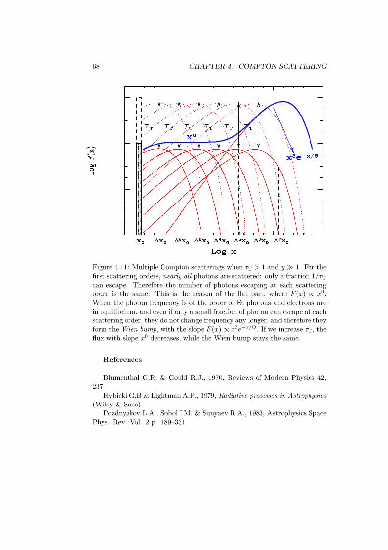
68 CHAPTER 4. COMPTON SCATTERING
Figure 4.11: Multiple Compton scatterings when τT > 1 and y ≫ 1. For thefirst scattering orders, nearly all photons are scattered: only a fraction 1/τTcan escape. Therefore the number of photons escaping at each scatteringorder is the same. This is the reason of the flat part, where F (x) ∝ x0.When the photon frequency is of the order of Θ, photons and electrons arein equilibrium, and even if only a small fraction of photon can escape at eachscattering order, they do not change frequency any longer, and therefore theyform the Wien bump, with the slope F (x) ∝ x3e−x/Θ. If we increase τT, theflux with slope x0 decreases, while the Wien bump stays the same.
References
Blumenthal G.R. & Gould R.J., 1970, Reviews of Modern Physics 42,237
Rybicki G.B & Lightman A.P., 1979, Radiative processes in Astrophysics
(Wiley & Sons)Pozdnyakov L.A., Sobol I.M. & Sunyaev R.A., 1983, Astrophysics Space
Phys. Rev. Vol. 2 p. 189–331

Chapter 5
Synchrotron Self–Compton
Consider a population of relativistic electrons in a magnetized region. Theywill produce synchrotron radiation, and therefore they will fill the regionwith photons. These synchrotron photons will have some probability tointeract again with the electrons, by the Inverse Compton process. Since theelectron “work twice” (first making synchrotron radiation, then scatteringit at higher energies) this particular kind of process is called synchrotronself–Compton, or SSC for short.
5.1 SSC emissivity
The importance of the scattering will of course be high if the densities ofelectrons and photons are large. If the electron distribution is a powerlaw [N(γ) = Kγ−p], then we expect that the SSC flux will be ∝ K2, i.e.quadratic in the electron density.
We should remember Eq. 4.52, and, instead of a generic Ur(ν), we shouldsubstitute the appropriate expression for the specific synchrotron radiationenergy density. We will then set:
Us(ν) =3R
4c
Ls(ν)
V= 4π
3R
4cǫs(ν) (5.1)
where 3R/(4c) is the average photon source–crossing time, and V is thevolume of the source. Now a simple trick: we write the specific synchrotronemissivity as
ǫs(ν) = ǫs,0 ν−α (5.2)
Remember: the α appearing here is the same index in Eq. 4.52. Substitutingthe above equations into Eq. 4.52 we have
ǫssc(νc) =(4/3)α−1
2τc ǫs,0ν
−αc
∫ νmax
νmin
dν
ν(5.3)
69
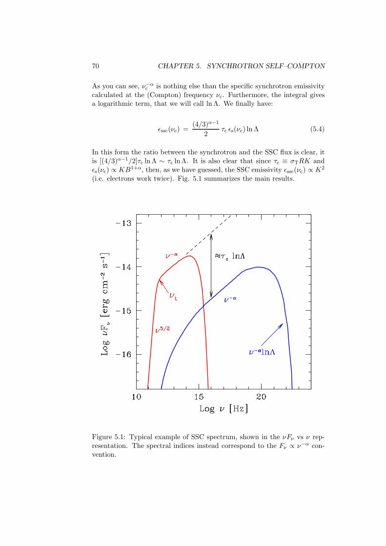
70 CHAPTER 5. SYNCHROTRON SELF–COMPTON
As you can see, ν−αc is nothing else than the specific synchrotron emissivity
calculated at the (Compton) frequency νc. Furthermore, the integral givesa logarithmic term, that we will call ln Λ. We finally have:
ǫssc(νc) =(4/3)α−1
2τc ǫs(νc) ln Λ (5.4)
In this form the ratio between the synchrotron and the SSC flux is clear, itis [(4/3)α−1/2]τc ln Λ ∼ τc ln Λ. It is also clear that since τc ≡ σTRK andǫs(νc) ∝ KB1+α, then, as we have guessed, the SSC emissivity ǫssc(νc) ∝ K2
(i.e. electrons work twice). Fig. 5.1 summarizes the main results.
Figure 5.1: Typical example of SSC spectrum, shown in the νFν vs ν rep-resentation. The spectral indices instead correspond to the Fν ∝ ν−α con-vention.

5.2. DIAGNOSTIC 71
5.2 Diagnostic
If we are confident that a the spectrum of a particular source is indeed givenby the SSC process, then we can use our theory to estimate a number ofphysical parameters. We have already stated (see Eq. 2.32) that observa-tions of the synchrotron spectrum in its self–absorbed part can yield thevalue of the magnetic field if we also know the angular radius of the source(if it is resolved). Observation in the thin part can then give us the productRK ≡ τc/σT (see Eq. 2.28). But τc is exactly what we need to predict thehigh energy flux produced by the SSC process. Note that if the source is re-solved (i.e. we know θs) we can get these information even without knowingthe distance of the source. To summarize:
F synthick(ν) ∝ θ2
s
ν5/2
B1/2→ get B
F synthin(ν) ∝ θ2
sRKB1+αν−α → get τc = RK/σT (5.5)
There is an even simpler case, which for reasons outlined below, is the mostcommon case employed when studying radio–loud AGNs. In fact, if youimagine to observe the source at the self absorption frequency νt, then youare both observing the thick and the thin flux at the same time. Then, letus call the flux at νt simply Ft. We can then re-write the equation above:
B ∝ θ4sν
5t
F 2t
τc ∝ Ftναt
θ2sB
1+α
Fssc(νc) ∝ τcFsyn(νc) ∝ τ2cB
1+αν−αc
∝ F2(2+α)t ν
−(5+3α)t θ−2(3+2α)
s ν−αc (5.6)
Once again: on the basis of a few observations of only the synchrotron flux,we can calculate what should be the SSC flux at the frequency νc. Note therather strong dependencies, particularly for θs, in the sense that the morecompact the source is, the larger the SSC flux.
If it happens that we do observe the source at high frequencies, wherewe expect that the SSC flux dominates, then we can check if our modelworks. Does it? For the strongest radio–loud sources, almost never. Thedisagreement between the predicted and the observed flux is really severe,we are talking of several orders of magnitude. Then either we are completelywrong about the model, or we miss some fundamental ingredient. We go forthe second option, since, after all, we do not find any mistake in our theory.
The missing ingredient is relativistic bulk motion. If the source is mov-ing towards us at relativistic velocities, we observe an enhanced flux andblueshifted frequencies. Not accounting for it, our estimates of the magnetic
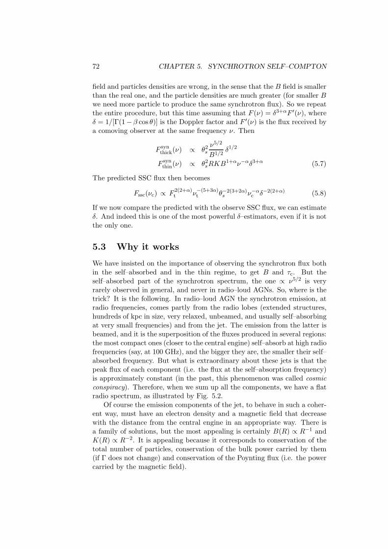
72 CHAPTER 5. SYNCHROTRON SELF–COMPTON
field and particles densities are wrong, in the sense that the B field is smallerthan the real one, and the particle densities are much greater (for smaller Bwe need more particle to produce the same synchrotron flux). So we repeatthe entire procedure, but this time assuming that F (ν) = δ3+αF ′(ν), whereδ = 1/[Γ(1−β cos θ)] is the Doppler factor and F ′(ν) is the flux received bya comoving observer at the same frequency ν. Then
F synthick(ν) ∝ θ2
s
ν5/2
B1/2δ1/2
F synthin(ν) ∝ θ2
sRKB1+αν−αδ3+α (5.7)
The predicted SSC flux then becomes
Fssc(νc) ∝ F2(2+α)t ν
−(5+3α)t θ−2(3+2α)
s ν−αc δ−2(2+α) (5.8)
If we now compare the predicted with the observe SSC flux, we can estimateδ. And indeed this is one of the most powerful δ–estimators, even if it is notthe only one.
5.3 Why it works
We have insisted on the importance of observing the synchrotron flux bothin the self–absorbed and in the thin regime, to get B and τc. But theself–absorbed part of the synchrotron spectrum, the one ∝ ν5/2 is veryrarely observed in general, and never in radio–loud AGNs. So, where is thetrick? It is the following. In radio–loud AGN the synchrotron emission, atradio frequencies, comes partly from the radio lobes (extended structures,hundreds of kpc in size, very relaxed, unbeamed, and usually self–absorbingat very small frequencies) and from the jet. The emission from the latter isbeamed, and it is the superposition of the fluxes produced in several regions:the most compact ones (closer to the central engine) self–absorb at high radiofrequencies (say, at 100 GHz), and the bigger they are, the smaller their self–absorbed frequency. But what is extraordinary about these jets is that thepeak flux of each component (i.e. the flux at the self–absorption frequency)is approximately constant (in the past, this phenomenon was called cosmic
conspiracy). Therefore, when we sum up all the components, we have a flatradio spectrum, as illustrated by Fig. 5.2.
Of course the emission components of the jet, to behave in such a coher-ent way, must have an electron density and a magnetic field that decreasewith the distance from the central engine in an appropriate way. There isa family of solutions, but the most appealing is certainly B(R) ∝ R−1 andK(R) ∝ R−2. It is appealing because it corresponds to conservation of thetotal number of particles, conservation of the bulk power carried by them(if Γ does not change) and conservation of the Poynting flux (i.e. the powercarried by the magnetic field).
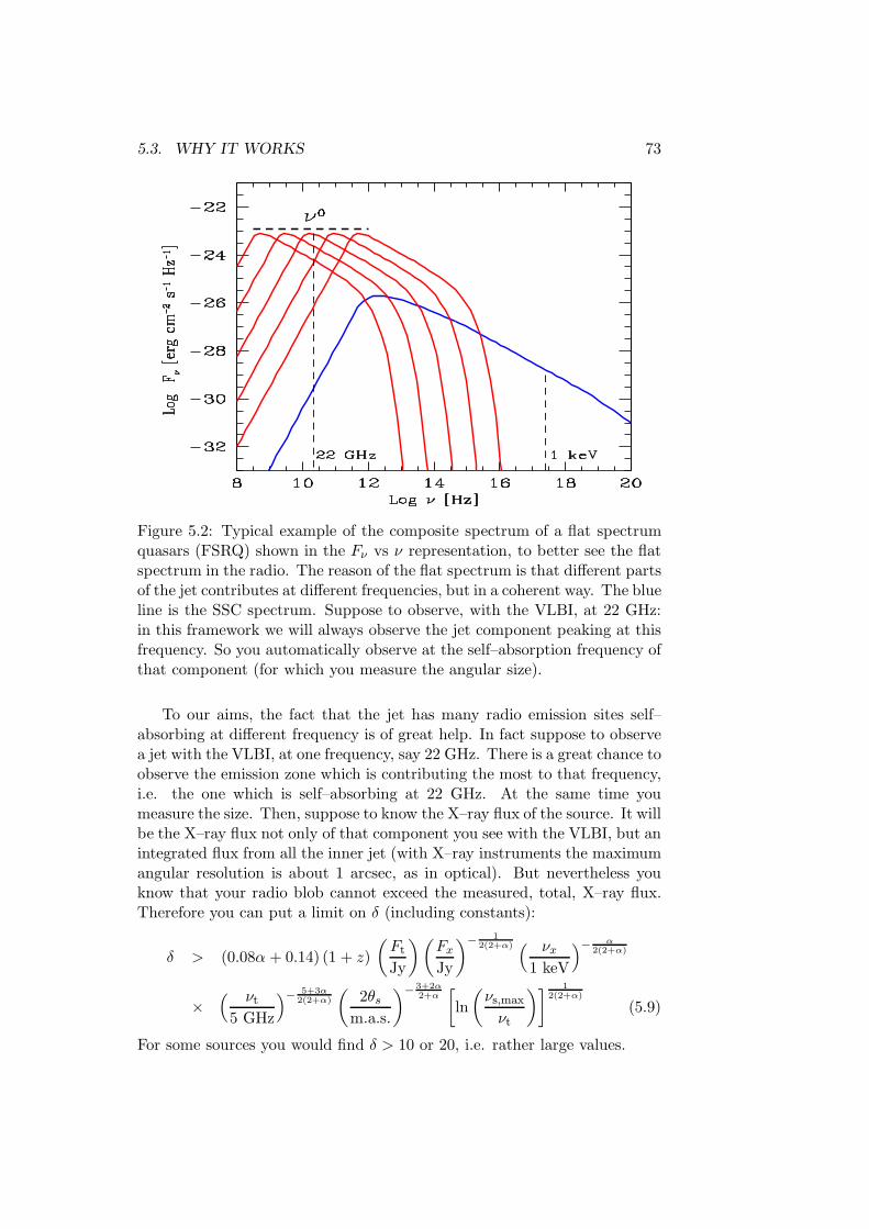
5.3. WHY IT WORKS 73
Figure 5.2: Typical example of the composite spectrum of a flat spectrumquasars (FSRQ) shown in the Fν vs ν representation, to better see the flatspectrum in the radio. The reason of the flat spectrum is that different partsof the jet contributes at different frequencies, but in a coherent way. The blueline is the SSC spectrum. Suppose to observe, with the VLBI, at 22 GHz:in this framework we will always observe the jet component peaking at thisfrequency. So you automatically observe at the self–absorption frequency ofthat component (for which you measure the angular size).
To our aims, the fact that the jet has many radio emission sites self–absorbing at different frequency is of great help. In fact suppose to observea jet with the VLBI, at one frequency, say 22 GHz. There is a great chance toobserve the emission zone which is contributing the most to that frequency,i.e. the one which is self–absorbing at 22 GHz. At the same time youmeasure the size. Then, suppose to know the X–ray flux of the source. It willbe the X–ray flux not only of that component you see with the VLBI, but anintegrated flux from all the inner jet (with X–ray instruments the maximumangular resolution is about 1 arcsec, as in optical). But nevertheless youknow that your radio blob cannot exceed the measured, total, X–ray flux.Therefore you can put a limit on δ (including constants):
δ > (0.08α + 0.14) (1 + z)
(
Ft
Jy
)(
Fx
Jy
)− 12(2+α) ( νx
1 keV
)− α
2(2+α)
×( νt
5 GHz
)− 5+3α
2(2+α)
(
2θs
m.a.s.
)− 3+2α
2+α[
ln
(
νs,max
νt
)]1
2(2+α)
(5.9)
For some sources you would find δ > 10 or 20, i.e. rather large values.