Bayesian methods for solving estimation and forecasting ...
160
Bayesian methods for solving estimation and forecasting problems in the high-frequency trading environment Paul Alexander Bilokon Christ Church University of Oxford A thesis submitted in partial fulfillment of the MSc in Mathematical Finance 16 December, 2016
Transcript of Bayesian methods for solving estimation and forecasting ...

Bayesian methods for solvingestimation and forecasting problems in
the high-frequency trading environment
Paul Alexander Bilokon
Christ Church
University of Oxford
A thesis submitted in partial fulfillment of the MSc in
Mathematical Finance
16 December, 2016

To God. And to my parents, Alex and Nataliya Bilokon. With love and gratitude.
To the memory of Rudolf Emil Kálmán (1930–2016),
who laid down the intellectual foundations on which this work is built.
i
Abstract
We examine modern stochastic filtering and Markov chain Monte Carlo (MCMC) methods and
consider their applications in finance, especially electronic trading.
Stochastic filtering methods have found many applications, from Space Shuttles to self-driving cars.
We review some classical and modern algorithms and show how they can be used to estimate and
forecast econometric models, stochastic volatility and term structure of risky bonds. We discuss the
practicalities, such as outlier filtering, parameter estimation, and diagnostics.
We focus on one particular application, stochastic volatility with leverage, and show how recent
advances in filtering methods can help in this application: kernel density estimation can be used
to estimate the predicted observation, filter out outliers, detect structural change, and improve the
root mean square error while preventing discontinuities due to the resampling step.
We then take a closer look at the discretisation of the continuous-time stochastic volatility models
and show how an alternative discretisation, based on what we call a filtering Euler–Maruyama
scheme, together with our generalisation of Gaussian assumed density filters to arbitrary (not nec-
essarily additive) correlated process and observation noises, gives rise to a new, very fast approxi-
mate filter for stochastic volatility with leverage. Its accuracy falls short of particle filters but beats
the unscented Kálmán filter. Due to its speed and reliance exclusively on scalar computations this
filter will be particularly useful in a high-frequency trading environment.
In the final chapter we examine the leverage effect in high-frequency trade data, using last data
point interpolation, tick and wall-clock time and generalise the models to take into account the
time intervals between the ticks.
We use a combination of MCMC methods and particle filtering methods. The robustness of the
latter helps estimate parameters and compute Bayes factors. The speed and precision of modern
filtering algorithms enables real-time filtering and prediction of the state.

Acknowledgements
First and foremost, I would like to thank my supervisor, Dan Jones, who not only taught and instructed me
academically, but also provided advice, guidance, and support in very challenging circumstances. Thank you
very much, Dan, for putting up with me during this project.
I would like to thank my mentors and former colleagues, Dan Crisan (Imperial College), Rob Smith (Citi-
group), William Osborn (formerly Citigroup), and Martin Zinkin (formerly Deutsche Bank), who have taught
me much of what I know about stochastic filtering. Rob not only taught me a lot, but was very helpful and
understanding when I was going through a difficult time. Martin showed me a level of scientific and software
development skill which I didn’t know existed. I would also like to thank my former manager at Deutsche
Bank, Jason Batt, for his help and encouragement. I am very grateful to my PhD supervisor, Abbas Edalat, and
scientific mentors, Claudio Albanese, Iain Clark, Achim Jung, Moe Hafiz, and Berc Rustem, for teaching me to
think scientifically.
I would also like to mention my quant and technology colleagues at Deutsche Bank Markets Electronic Trading
who all, one way or another, taught me various aspects of the science, technology, and business of electronic
trading: Tahsin Alam, Zar Amrolia, Benedict Carter, Teddy Cho, Luis Cota, Matt Daly, Madhucchand Darbha,
Alex Doran, Marina Duma, Gareth Evans, Brian Gabillet, Yelena Gilbert, Thomas Giverin, Hakan Guney,
James Gwinnutt, William Hall, Matt Harvey, Mridula Iyer, Chris-M Jones, Sergey Korovin, Egor Kraev,
Leonid Kraginskiy, Peter Lee, Ewan Lowe, Phil Morris, Ian Muetzelfeldt, Roel Oomen, Helen O’Regan, Kir-
ill Petunin, Stanislav Pustygin, Claude Rosenstrauch, Lubomir Schmidt, Torsten Schöneborn, Sumit Sengupta,
Alexander Stepanov, Viktoriya Stepanova, Ian Thomson, Krzysztof Zylak. It has been an honour and privilege
to work with you all while I was writing this dissertation.
My friends have provided the much-needed encouragement and support: Sofiko Abanoidze, John and
Anastasia Aston, Ester Goldberg, James Gwinnutt, Moe Hafiz, Lyudmila Meshchersky, Laly Nickatsadze,
Adel Sabirova, Stephen Scott, Andrei Serjantov, Irakli Shanidze, Ed Silantyev, Nitza and Robin Spiro,
Natasha Svetlova, Alexey Taycher, Nataliya Tkachuk, Jay See Tow, Douglas Vieira.
Finally, I would like to acknowledge Saeed Amen, Matthew Dixon, Attila Agod, and Jan Novotny at Thale-
sians, who have not only been great colleagues, but also great friends. I am especially grateful to Saeed for his
patience, support, and friendship over the years.
iii

Nomenclature
the Halmos symbol, which stands for quod erat demonstrandum
A := 1, 2, 3 is equal by definition to (left to right)
1, 2, 3 =: A is equal by definition to (right to left)
N natural numbers
N0 ditto, explicitly incl. 0
N∗ nonzero natural numbers
R reals, (−∞,+∞)
R+ positive reals, (0,+∞)
R+0 nonnegative reals, [0,+∞)
R+0 extended nonnegative reals, [0,+∞]
F ,G, . . . name of a collection
A, B, . . . name of a set
A, B, . . . definition of a collection
O ∈ T | O clopen —"—
1, 2, 3 definition of a set
x ∈N | x even —"—
(ak) name of element of a sequence
(ak)k∈N —"—
(ak)∞k=1 —"—
(2, 4, 6, . . .) definition of a sequence
(2, 4, 6) definition of a tuple
x ∈N | x even such that
iv

Z ⊆ R subset
R ⊇ Z superset
Z ( R proper subset
R ) Z proper superset
A× B the Cartesian product of the sets A and B
C→ R+0 function type
f : C→ R+0 —"—
x 7→ x2 function definition
f : x 7→ x2 —"—
f (A) the image of the set A under the function f
f−1(A) the inverse image of the set A under the function f
‖x‖p p-norm; in particular, when p = 2, Euclidean norm
v name of a vector
A name of a matrix
vᵀ transpose
vec A vectorisation of a matrix
σ(A) the σ-algebra generated by the family of sets A
p(· | ·) a generic conditional probability density or mass function, with the arguments making
it clear which conditional distribution it relates to
T the time set
X in the context of filtering, the state process
S the state space
B(S) the Borel σ-algebra of S
X t∈T the usual augmentation of the filtration generated by X
U (a, b) continuous uniform distribution with support [a, b]
N(µ, σ2) univariate normal (Gaussian) distribution with mean µ and variance σ2
N (µ, Σ) multivariate normal (Gaussian) distribution with mean µ and covariance matrix Σ
v
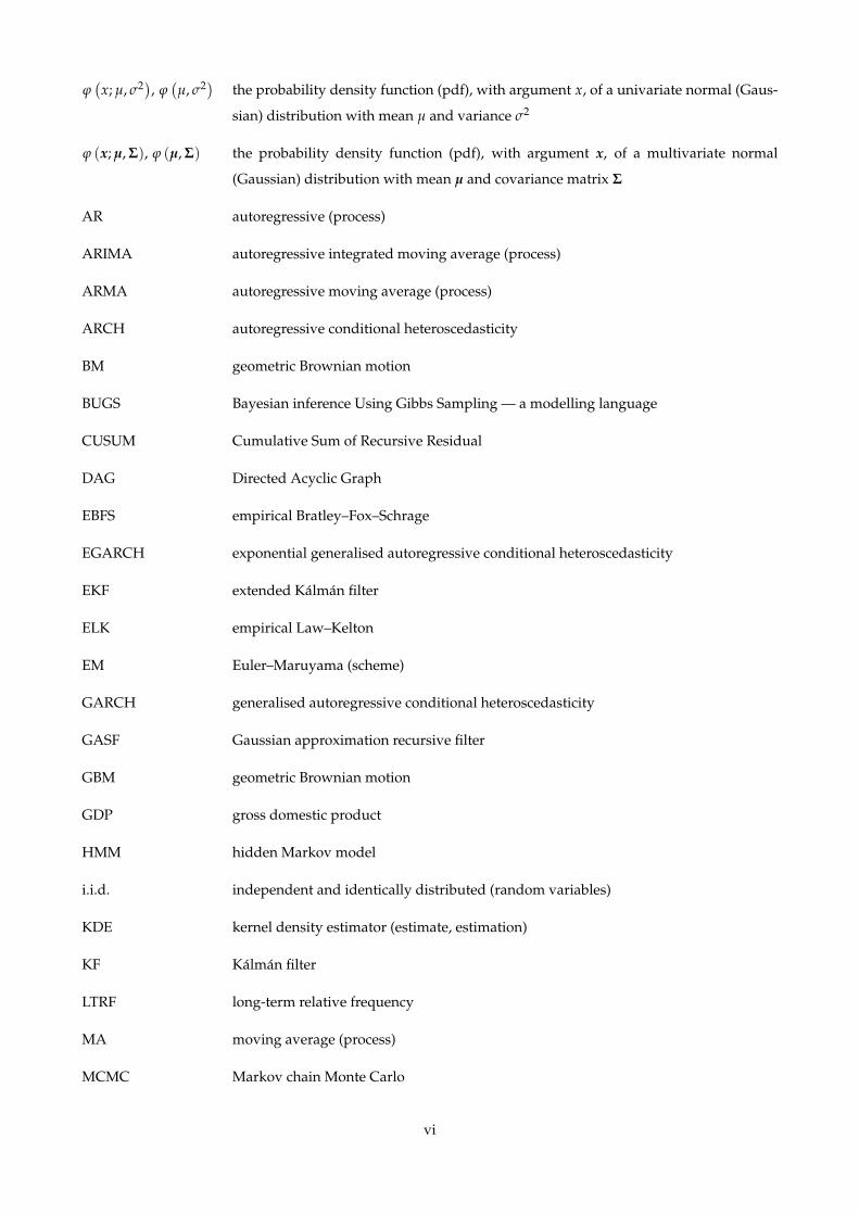
ϕ(
x; µ, σ2), ϕ(µ, σ2) the probability density function (pdf), with argument x, of a univariate normal (Gaus-
sian) distribution with mean µ and variance σ2
ϕ (x; µ, Σ), ϕ (µ, Σ) the probability density function (pdf), with argument x, of a multivariate normal
(Gaussian) distribution with mean µ and covariance matrix Σ
AR autoregressive (process)
ARIMA autoregressive integrated moving average (process)
ARMA autoregressive moving average (process)
ARCH autoregressive conditional heteroscedasticity
BM geometric Brownian motion
BUGS Bayesian inference Using Gibbs Sampling — a modelling language
CUSUM Cumulative Sum of Recursive Residual
DAG Directed Acyclic Graph
EBFS empirical Bratley–Fox–Schrage
EGARCH exponential generalised autoregressive conditional heteroscedasticity
EKF extended Kálmán filter
ELK empirical Law–Kelton
EM Euler–Maruyama (scheme)
GARCH generalised autoregressive conditional heteroscedasticity
GASF Gaussian approximation recursive filter
GBM geometric Brownian motion
GDP gross domestic product
HMM hidden Markov model
i.i.d. independent and identically distributed (random variables)
KDE kernel density estimator (estimate, estimation)
KF Kálmán filter
LTRF long-term relative frequency
MA moving average (process)
MCMC Markov chain Monte Carlo
vi

MISE mean integrated square error
MLE maximum likelihood estimator (estimate, estimation)
MMSE minimum mean square error estimator (estimate, estimation)
MSE mean square error
NLN normal–lognormal mixture (distribution)
OU Ornstein-Uhlenbeck (process)
post-RPF post-regularised particle filter
QML quasi-maximum likelihood
RMSE root mean square error
SDE stochastic differential equation
SIR sequential importance resampling
SIS sequential importance sampling
SISR sequential importance sampling with resampling
SMC sequential Monte Carlo
SV stochastic volatilty
SVL stochastic volatility with leverage
SVL2 stochastic volatility with the second correlation structure
SVLJ stochastic volatility with leverage and jumps
UKF unscented Kálmán filter
wcSVL wall-clock stochastic volatility with leverage
Z-spread zero volatility spread
vii

Contents
Nomenclature iv
Contents vii
List of tables xi
List of figures xii
List of algorithms xiv
List of listings xv
Preface xvii
1 Volatility 1
1.1 Introduction . . . . . . . . . . . . . . . . . . . . . . . . . . . . . . . . . . . . . . . . . . . . . . . . . 1
1.2 The early days of volatility modelling: constant volatility models . . . . . . . . . . . . . . . . . . 1
1.3 Evidence against the constant volatility assumption . . . . . . . . . . . . . . . . . . . . . . . . . . 2
1.4 The two families of models . . . . . . . . . . . . . . . . . . . . . . . . . . . . . . . . . . . . . . . . 3
1.4.1 The GARCH family . . . . . . . . . . . . . . . . . . . . . . . . . . . . . . . . . . . . . . . . 3
1.4.2 The stochastic volatility family . . . . . . . . . . . . . . . . . . . . . . . . . . . . . . . . . . 4
1.5 The statistical leverage effect . . . . . . . . . . . . . . . . . . . . . . . . . . . . . . . . . . . . . . . . 6
1.6 A stochastic volatility model with leverage and jumps . . . . . . . . . . . . . . . . . . . . . . . . . 6
1.7 Conclusions and further reading . . . . . . . . . . . . . . . . . . . . . . . . . . . . . . . . . . . . . 9
viii

2 The filtering framework 11
2.1 Introduction . . . . . . . . . . . . . . . . . . . . . . . . . . . . . . . . . . . . . . . . . . . . . . . . . 11
2.2 Special case: general state-space models . . . . . . . . . . . . . . . . . . . . . . . . . . . . . . . . . 13
2.3 Particle filtering methods . . . . . . . . . . . . . . . . . . . . . . . . . . . . . . . . . . . . . . . . . 13
2.4 Applying the particle filter to the stochastic volatility model with leverage and jumps . . . . . . 15
2.5 The Kálmán filter . . . . . . . . . . . . . . . . . . . . . . . . . . . . . . . . . . . . . . . . . . . . . . 18
2.6 Some examples of linear-Gaussian state space models . . . . . . . . . . . . . . . . . . . . . . . . . 19
2.6.1 A non-financial example: the Newtonian system . . . . . . . . . . . . . . . . . . . . . . . . 20
2.6.2 Autoregressive moving average models . . . . . . . . . . . . . . . . . . . . . . . . . . . . . 20
2.6.3 Continuous-time stochastic processes: the Wiener process, geometric Brownian motion,
and the Ornstein–Uhlenbeck process . . . . . . . . . . . . . . . . . . . . . . . . . . . . . . . 21
2.7 The extended Kálmán filter . . . . . . . . . . . . . . . . . . . . . . . . . . . . . . . . . . . . . . . . 24
2.8 An example application of the extended Kálmán filter: modelling credit spread . . . . . . . . . . 25
2.9 Outlier detection in (extended) Kálmán filtering . . . . . . . . . . . . . . . . . . . . . . . . . . . . 26
2.10 Gaussian assumed density filtering . . . . . . . . . . . . . . . . . . . . . . . . . . . . . . . . . . . . 27
2.11 Parameter estimation . . . . . . . . . . . . . . . . . . . . . . . . . . . . . . . . . . . . . . . . . . . . 28
2.12 Relationship with Markov chain Monte Carlo methods . . . . . . . . . . . . . . . . . . . . . . . . 30
2.13 Prediction . . . . . . . . . . . . . . . . . . . . . . . . . . . . . . . . . . . . . . . . . . . . . . . . . . 31
2.14 Diagnostics . . . . . . . . . . . . . . . . . . . . . . . . . . . . . . . . . . . . . . . . . . . . . . . . . . 32
2.15 Conclusions and further reading . . . . . . . . . . . . . . . . . . . . . . . . . . . . . . . . . . . . . 33
3 Stochastic filtering and MCMC analysis of stochastic volatility models with leverage 34
3.1 Introduction . . . . . . . . . . . . . . . . . . . . . . . . . . . . . . . . . . . . . . . . . . . . . . . . . 34
3.2 SVL as a discretisation of a continuous-time model . . . . . . . . . . . . . . . . . . . . . . . . . . . 34
3.3 Validation of the SVL2 model . . . . . . . . . . . . . . . . . . . . . . . . . . . . . . . . . . . . . . . 36
3.3.1 Normal–lognormal (NLN) mixture distribution . . . . . . . . . . . . . . . . . . . . . . . . 36
3.3.2 Martingality . . . . . . . . . . . . . . . . . . . . . . . . . . . . . . . . . . . . . . . . . . . . . 37
3.3.3 The discretisation scheme . . . . . . . . . . . . . . . . . . . . . . . . . . . . . . . . . . . . . 37
3.3.4 MCMC Analysis of SVL and SVL2 . . . . . . . . . . . . . . . . . . . . . . . . . . . . . . . . 38
3.4 Particle filtering for SVL2 . . . . . . . . . . . . . . . . . . . . . . . . . . . . . . . . . . . . . . . . . 39
3.5 Conclusions, further work, and further reading . . . . . . . . . . . . . . . . . . . . . . . . . . . . . 42
ix

4 Extensions of the filtering methods 43
4.1 Predicted observation distribution for particle filters . . . . . . . . . . . . . . . . . . . . . . . . . . 43
4.2 Jumps or outliers? . . . . . . . . . . . . . . . . . . . . . . . . . . . . . . . . . . . . . . . . . . . . . . 44
4.3 Detecting structural change . . . . . . . . . . . . . . . . . . . . . . . . . . . . . . . . . . . . . . . . 44
4.4 Resampling . . . . . . . . . . . . . . . . . . . . . . . . . . . . . . . . . . . . . . . . . . . . . . . . . 45
4.5 A generalisation of the Gaussian filter . . . . . . . . . . . . . . . . . . . . . . . . . . . . . . . . . . 47
4.6 An application of the Gaussian filter to SVL2 . . . . . . . . . . . . . . . . . . . . . . . . . . . . . . 48
4.7 Conclusions, further work, and further reading . . . . . . . . . . . . . . . . . . . . . . . . . . . . . 49
5 Intraday stochastic volatility with leverage 51
5.1 Introduction . . . . . . . . . . . . . . . . . . . . . . . . . . . . . . . . . . . . . . . . . . . . . . . . . 51
5.2 Leverage effect in intraday data . . . . . . . . . . . . . . . . . . . . . . . . . . . . . . . . . . . . . . 51
5.3 Trade time or wall clock time? . . . . . . . . . . . . . . . . . . . . . . . . . . . . . . . . . . . . . . . 53
5.4 Conclusions, further work, and further reading . . . . . . . . . . . . . . . . . . . . . . . . . . . . . 54
Conclusions and further work 55
A Proofs 56
A.1 Introduction . . . . . . . . . . . . . . . . . . . . . . . . . . . . . . . . . . . . . . . . . . . . . . . . . 56
A.2 Proofs for Chapter 3 . . . . . . . . . . . . . . . . . . . . . . . . . . . . . . . . . . . . . . . . . . . . . 56
A.3 Proofs for Chapter 4 . . . . . . . . . . . . . . . . . . . . . . . . . . . . . . . . . . . . . . . . . . . . . 59
B Derivation of the Gaussian filter for the Jacquier–Polson–Rossi model 61
C Description of the datasets used in empirical work 63
C.1 Introduction . . . . . . . . . . . . . . . . . . . . . . . . . . . . . . . . . . . . . . . . . . . . . . . . . 63
C.2 Financial quantities . . . . . . . . . . . . . . . . . . . . . . . . . . . . . . . . . . . . . . . . . . . . . 63
C.3 Datasets . . . . . . . . . . . . . . . . . . . . . . . . . . . . . . . . . . . . . . . . . . . . . . . . . . . 65
C.4 Summary and further reading . . . . . . . . . . . . . . . . . . . . . . . . . . . . . . . . . . . . . . . 67
x

D An overview of frequentist and Bayesian approaches to estimation 68
D.1 Introduction . . . . . . . . . . . . . . . . . . . . . . . . . . . . . . . . . . . . . . . . . . . . . . . . . 68
D.2 Interpretations of probability . . . . . . . . . . . . . . . . . . . . . . . . . . . . . . . . . . . . . . . 68
D.3 Bayes’s theorem . . . . . . . . . . . . . . . . . . . . . . . . . . . . . . . . . . . . . . . . . . . . . . . 69
D.4 Frequentist and Bayesian estimation . . . . . . . . . . . . . . . . . . . . . . . . . . . . . . . . . . . 69
D.5 Further reading . . . . . . . . . . . . . . . . . . . . . . . . . . . . . . . . . . . . . . . . . . . . . . . 70
E Markov chain Monte Carlo analyses in OpenBUGS: implementations, instructions, and results 71
E.1 Introduction . . . . . . . . . . . . . . . . . . . . . . . . . . . . . . . . . . . . . . . . . . . . . . . . . 71
E.2 Implementation of the models in BUGS . . . . . . . . . . . . . . . . . . . . . . . . . . . . . . . . . 71
E.3 Instructions for running Markov chain Monte Carlo analyses in OpenBUGS . . . . . . . . . . . . 74
E.4 Output analysis and diagnostics with coda . . . . . . . . . . . . . . . . . . . . . . . . . . . . . . . 77
E.5 Results . . . . . . . . . . . . . . . . . . . . . . . . . . . . . . . . . . . . . . . . . . . . . . . . . . . . 78
E.5.1 Summaries: node statistics . . . . . . . . . . . . . . . . . . . . . . . . . . . . . . . . . . . . 78
E.5.2 Selected OpenBUGS plots . . . . . . . . . . . . . . . . . . . . . . . . . . . . . . . . . . . . . 82
F Results of running stochastic filters 98
Bibliography 111
Indices 128
Subject Index . . . . . . . . . . . . . . . . . . . . . . . . . . . . . . . . . . . . . . . . . . . . . . . . . . . . 129
Index of Authors . . . . . . . . . . . . . . . . . . . . . . . . . . . . . . . . . . . . . . . . . . . . . . . . . 133
xi

List of Tables
3.1 The means of the posteriors of the model parameters for SVL and SVL2 obtained after running
the MCMC simulations for each dataset . . . . . . . . . . . . . . . . . . . . . . . . . . . . . . . . . 41
3.2 A comparison between the SVL and SVL2 models on daily datasets . . . . . . . . . . . . . . . . . 41
4.1 A comparison between different stochastic filters applied to generated SVL data . . . . . . . . . 50
C.1 Summary of the datasets . . . . . . . . . . . . . . . . . . . . . . . . . . . . . . . . . . . . . . . . . . 67
xii

List of Figures
1.1 An example of the SVLJ data generated using StateSpaceModelDataGenerator of the BayesTSA
library . . . . . . . . . . . . . . . . . . . . . . . . . . . . . . . . . . . . . . . . . . . . . . . . . . . . 8
1.2 The two conventions used in designating disturbances (noises) in econometric models and the
two different correlation structures between the disturbances . . . . . . . . . . . . . . . . . . . . . 9
2.1 The result of applying Algorithm 5.1 to the generated SVLJ data . . . . . . . . . . . . . . . . . . . 17
2.2 An ARMA(2, 1) time series generated using StateSpaceModelDataGenerator of the BayesTSA
library . . . . . . . . . . . . . . . . . . . . . . . . . . . . . . . . . . . . . . . . . . . . . . . . . . . . 21
2.3 The result of applying the Kálmán filter (Algorithm 2.4) to the noisy observation in Figure 2.2 . . 22
4.1 Comparison of the RMSE for different outlier detection thresholds . . . . . . . . . . . . . . . . . 45
4.2 Comparison of the RMSE after running the filter with the smooth and post-RPF resampling
schemes . . . . . . . . . . . . . . . . . . . . . . . . . . . . . . . . . . . . . . . . . . . . . . . . . . . 46
5.1 A visual representation of some of the results of Table 3.1 for the SVL model . . . . . . . . . . . . 52
5.2 A visual representation of the results of applying the SVL and SVL2 models to intraday data . . 53
E.1 Posterior density for model SV, Dataset 1 . . . . . . . . . . . . . . . . . . . . . . . . . . . . . . . . 83
E.2 Posterior density for model SVL, Dataset 1 . . . . . . . . . . . . . . . . . . . . . . . . . . . . . . . 84
E.3 Posterior density for model SVL2, Dataset 1 . . . . . . . . . . . . . . . . . . . . . . . . . . . . . . . 85
E.4 Posterior density for model SV, Dataset 2 . . . . . . . . . . . . . . . . . . . . . . . . . . . . . . . . 86
E.5 Posterior density for model SVL, Dataset 2 . . . . . . . . . . . . . . . . . . . . . . . . . . . . . . . 87
E.6 Posterior density for model SVL2, Dataset 2 . . . . . . . . . . . . . . . . . . . . . . . . . . . . . . . 88
E.7 Posterior density for model SVL, Dataset 6 . . . . . . . . . . . . . . . . . . . . . . . . . . . . . . . 89
E.8 Posterior density for model SVL2, Dataset 6 . . . . . . . . . . . . . . . . . . . . . . . . . . . . . . . 90
E.9 Posterior density for model SVL, Dataset 7 . . . . . . . . . . . . . . . . . . . . . . . . . . . . . . . 91
E.10 Posterior density for model SVL2, Dataset 7 . . . . . . . . . . . . . . . . . . . . . . . . . . . . . . . 92
xiii

E.11 Posterior density for model SVL, Dataset 8 . . . . . . . . . . . . . . . . . . . . . . . . . . . . . . . 93
E.12 Posterior density for model SVL2, Dataset 8 . . . . . . . . . . . . . . . . . . . . . . . . . . . . . . . 94
E.13 Posterior density for model SVL, Dataset 12 . . . . . . . . . . . . . . . . . . . . . . . . . . . . . . . 95
E.14 Posterior density for model SVL2, Dataset 12 . . . . . . . . . . . . . . . . . . . . . . . . . . . . . . 96
E.15 The analogues of Figure 5.2 for the remaining dataset/model combinations . . . . . . . . . . . . 97
F.1 The result of running the Harvey–Shephard Kálmán filter with ρ = −0.8 in Table 4.1 . . . . . . . 99
F.2 The result of running the modified UKF with ρ = −0.8 in Table 4.1 . . . . . . . . . . . . . . . . . 100
F.3 The result of running the generalised Gaussian filter with ρ = −0.8 in Table 4.1 . . . . . . . . . . 101
F.4 The result of running the particle filter for SVL2, post-RPF resampling, 300 particles, with ρ =
−0.8 in Table 4.1 . . . . . . . . . . . . . . . . . . . . . . . . . . . . . . . . . . . . . . . . . . . . . . . 102
F.5 The result of running the particle filter for SVL, post-RPF resampling, 300 particles, with ρ =
−0.8 in Table 4.1 . . . . . . . . . . . . . . . . . . . . . . . . . . . . . . . . . . . . . . . . . . . . . . . 103
F.6 The result of running the Harvey–Shephard Kálmán filter with ρ = −0.5 in Table 4.1 . . . . . . . 104
F.7 The result of running the modified UKF with ρ = −0.5 in Table 4.1 . . . . . . . . . . . . . . . . . 105
F.8 The result of running the generalised Gaussian filter with ρ = −0.5 in Table 4.1 . . . . . . . . . . 106
F.9 The result of running the particle filter for SVL2, post-RPF resampling, 300 particles, with ρ =
−0.5 in Table 4.1 . . . . . . . . . . . . . . . . . . . . . . . . . . . . . . . . . . . . . . . . . . . . . . . 107
F.10 The result of running the particle filter for SVL, post-RPF resampling, 300 particles, with ρ =
−0.5 in Table 4.1 . . . . . . . . . . . . . . . . . . . . . . . . . . . . . . . . . . . . . . . . . . . . . . . 108
xiv

List of Algorithms
2.1 Particle filter: sequential importance resampling (SIR) . . . . . . . . . . . . . . . . . . . . . . . . . 14
2.2 Multinomial resampling . . . . . . . . . . . . . . . . . . . . . . . . . . . . . . . . . . . . . . . . . . 15
2.3 An adaptation of the particle filter (Algorithm 2.1) developed by Pitt et al. for the SVLJ model . . 16
2.4 Kálmán filter . . . . . . . . . . . . . . . . . . . . . . . . . . . . . . . . . . . . . . . . . . . . . . . . . 18
2.5 Extended Kálmán filter . . . . . . . . . . . . . . . . . . . . . . . . . . . . . . . . . . . . . . . . . . . 25
2.6 Gaussian moment matching approximation of a possibly non-additive transform . . . . . . . . . 27
2.7 Gaussian filter with possibly non-additive noise . . . . . . . . . . . . . . . . . . . . . . . . . . . . 28
3.1 An adaptation of the particle filter (Algorithm 2.1) for the SVL2 model . . . . . . . . . . . . . . . 40
4.1 Resampling in the post-regularised particle filter (post-RPF) . . . . . . . . . . . . . . . . . . . . . 46
4.2 Generalised Gaussian moment matching approximation . . . . . . . . . . . . . . . . . . . . . . . 47
4.3 Generalised Gaussian filter . . . . . . . . . . . . . . . . . . . . . . . . . . . . . . . . . . . . . . . . 48
4.4 Generalised Gaussian filter for SVL2 . . . . . . . . . . . . . . . . . . . . . . . . . . . . . . . . . . . 49
5.1 An adaptation of the particle filter Algorithm 5.1 to wcSVL . . . . . . . . . . . . . . . . . . . . . . 54
B.1 Generalised Gaussian filter for the Jacquier–Polson–Rossi model . . . . . . . . . . . . . . . . . . . 62
xv

Listings
E.1 An implementation of the SV model in BUGS . . . . . . . . . . . . . . . . . . . . . . . . . . . . . . 71
E.2 An implementation of the SVL model in BUGS . . . . . . . . . . . . . . . . . . . . . . . . . . . . . 72
E.3 An implementation of the SVL2 model in BUGS . . . . . . . . . . . . . . . . . . . . . . . . . . . . 72
E.4 An implementation of the wcSVL model in BUGS . . . . . . . . . . . . . . . . . . . . . . . . . . . 73
E.5 Node statistics for model SV, Dataset 1 . . . . . . . . . . . . . . . . . . . . . . . . . . . . . . . . . . 78
E.6 Node statistics for model SVL, Dataset 1 . . . . . . . . . . . . . . . . . . . . . . . . . . . . . . . . . 78
E.7 Node statistics for model SVL2, Dataset 1 . . . . . . . . . . . . . . . . . . . . . . . . . . . . . . . . 78
E.8 Node statistics for model SV, Dataset 2 . . . . . . . . . . . . . . . . . . . . . . . . . . . . . . . . . . 78
E.9 Node statistics for model SVL, Dataset 2 . . . . . . . . . . . . . . . . . . . . . . . . . . . . . . . . . 78
E.10 Node statistics for model SVL2, Dataset 2 . . . . . . . . . . . . . . . . . . . . . . . . . . . . . . . . 78
E.11 Node statistics for model SVL, Dataset 3 . . . . . . . . . . . . . . . . . . . . . . . . . . . . . . . . . 79
E.12 Node statistics for model SVL2, Dataset 3 . . . . . . . . . . . . . . . . . . . . . . . . . . . . . . . . 79
E.13 Node statistics for model SVL, Dataset 4 . . . . . . . . . . . . . . . . . . . . . . . . . . . . . . . . . 79
E.14 Node statistics for model SVL2, Dataset 4 . . . . . . . . . . . . . . . . . . . . . . . . . . . . . . . . 79
E.15 Node statistics for model SVL, Dataset 5 . . . . . . . . . . . . . . . . . . . . . . . . . . . . . . . . . 79
E.16 Node statistics for model SVL2, Dataset 5 . . . . . . . . . . . . . . . . . . . . . . . . . . . . . . . . 79
E.17 Node statistics for model SVL, Dataset 6 . . . . . . . . . . . . . . . . . . . . . . . . . . . . . . . . . 79
E.18 Node statistics for model SVL2, Dataset 6 . . . . . . . . . . . . . . . . . . . . . . . . . . . . . . . . 80
E.19 Node statistics for model SVL, Dataset 7 . . . . . . . . . . . . . . . . . . . . . . . . . . . . . . . . . 80
E.20 Node statistics for model SVL2, Dataset 7 . . . . . . . . . . . . . . . . . . . . . . . . . . . . . . . . 80
E.21 Node statistics for model SVL, Dataset 8 . . . . . . . . . . . . . . . . . . . . . . . . . . . . . . . . . 80
E.22 Node statistics for model SVL2, Dataset 8 . . . . . . . . . . . . . . . . . . . . . . . . . . . . . . . . 80
E.23 Node statistics for model SVL, Dataset 9 . . . . . . . . . . . . . . . . . . . . . . . . . . . . . . . . . 80
E.24 Node statistics for model SVL2, Dataset 9 . . . . . . . . . . . . . . . . . . . . . . . . . . . . . . . . 81
xvi

E.25 Node statistics for model SVL, Dataset 10 . . . . . . . . . . . . . . . . . . . . . . . . . . . . . . . . 81
E.26 Node statistics for model SVL2, Dataset 10 . . . . . . . . . . . . . . . . . . . . . . . . . . . . . . . 81
E.27 Node statistics for model SVL, Dataset 11 . . . . . . . . . . . . . . . . . . . . . . . . . . . . . . . . 81
E.28 Node statistics for model SVL2, Dataset 11 . . . . . . . . . . . . . . . . . . . . . . . . . . . . . . . 81
E.29 Node statistics for model SVL, Dataset 12 . . . . . . . . . . . . . . . . . . . . . . . . . . . . . . . . 81
E.30 Node statistics for model SVL2, Dataset 12 . . . . . . . . . . . . . . . . . . . . . . . . . . . . . . . 81
E.31 Node statistics for model SVL, Dataset 13 . . . . . . . . . . . . . . . . . . . . . . . . . . . . . . . . 82
E.32 Node statistics for model SVL2, Dataset 13 . . . . . . . . . . . . . . . . . . . . . . . . . . . . . . . 82
xvii

Preface
Overview
Time-varying volatility was mentioned as early as 1915 [Mit15] and has been at the centre of attention ever
since the emergence of mathematical finance in the 1960s and 70s [Man63, BS72]. The numerous models that
have been developed to account for the empirically observed stylised facts can be divided into two families:
the ARCH/GARCH family, originating in [Eng82, Bol86], and the stochastic volatility (SV) family, originating
in [Cla73, TP83, Tay82, HW87]. Both families remain actively researched and used to this day: see [EFF08] and
[GHR96, She96, She05], respectively, for overviews. Arguments have been heard in favour of both approaches.
The author’s professional interest is in applications to medium- and high-frequency trading. As we shall see
in Chapter 1, the merits of the SV models are particularly attractive in this setting, so we shall restrict our focus
to the SV family.
The leverage effect [BS73], irrespective of whether or not it is due to leverage [FW00, HL11], is a well-known
stylised fact in the empirical finance literature. Its existence and practical significance are confirmed by the
author’s own trading experience. We shall therefore consider those modifications of the classical SV model
that incorporate the leverage effect.
Several recent papers have shown how modern Bayesian methods — Markov chain Monte Carlo [MY00, Yu05]
and particle filtering [MP09, MP11a, MP11b, PMD14] — can be applied to the filtering and forecasting of
stochastic volatility models, including those incorporating leverage. In this dissertation we shall build upon
these advances.
It is with a view towards addressing these concerns that we embark on the present work. As a by-product,
we seek to contribute to the body of knowledge in the theory and practice of Bayesian methods, especially
stochastic filtering. This is a worthwhile end in itself, since such methods have many applications outside
finance [Sim06].
We also aim to develop a better understanding of the leverage effect in the high-frequency setting. While
there have been recent studies in this area [Lit04, BLT06, ASFL13], to the best of our knowledge, none of them
utilised the Bayesian methods that we consider in this work.
xviii

Notation and conventions
Throughout the text the author (Paul Bilokon) uses the author’s “we”. When referring to other researchers in
our work we use their full names on the first occurrence, then only surnames on subsequent occurrences.
For the reader’s convenience we have included a nomenclature listing the symbols and abbreviations used in
this work. It precedes the table of contents and this preface. We have tried to keep the notation as standard as
possible, while unifying it across the entire work.
Throughout this work, we shall use only natural logarithms, i.e. those with base e, and, in order to be explicit,
we shall denote them by ln, e.g. ln x.
To avoid ambiguity due to locale differences, we shall always use the notation “YYYY.MM.DD” for all dates,
for example, “2015.07.20” will represent the 20th June, 2015.
Plan of the dissertation
We open the dissertation with a selective review of classical and recent literature on time-varying volatility,
introduce the leverage effect, and summarise recent research on stochastic volatility models with leverage and
jumps (Chapter 1). We then review the stochastic filtering framework, focussing on algorithms and practi-
calities, and mention examples of applying the filtering framework in finance and trading (Chapter 2). In
the same chapter we very briefly introduce Markov chain Monte Carlo (MCMC) methods (Section 2.12) and
explain how they are related to filtering. We describe how particle filtering (Section 2.4) and MCMC (Sec-
tion 2.12) have been applied to a stochastic volatility model incorporating leverage in academic literature. In
Chapter 3 we consider this in more detail. Following [Yu05], we examine this model as a particular discreti-
sation of continuous-time stochastic volatility model and use MCMC and particle filtering to compare it with
an alternative discretisation. In this chapter we employ Bayesian techniques of [KSC98, Yu05] for comparing
econometric models. We then proceed to introduce some investigate some extensions from recent literature on
stochastic filtering in application to stochastic volatility with leverage (Chapter 4). Finally, in Chapter 5, we
use MCMC techniques to examine leverage effect intraday, using high-frequency data.
We had to balance the conflicting requirements of making this dissertation both concise and self-contained.
Each chapter ends with a section summarising the findings and citing further references to the literature. Some
material has been relegated to the appendices. For example, proofs of mathematical propositions are given in
Appendix A rather than in the body of the dissertation, so they don’t interrupt the flow of the discussion. In
Chapter 4 we derive a Gaussian filter for the SVL2 model. For completeness, we give a similar derivation for
the Jacquier–Polson–Rossi model [JPR04] in Appendix B.
Appendix C contains detailed descriptions of the datasets that we used in empirical work. We shall refer to
all datasets using the notation “Dataset N”, N ∈ N∗. In brief, we have used 15 datasets in empirical work.
Datasets 1–13 consist of daily log-returns (respectively: GBP/USD spot, S&P 500 index 1980–1987, S&P 500
index 1988–1995, S&P 500 index 1996–2003, S&P 500 index 2004–2011, S&P 500 index 2012–2016, FTSE 100
xix

index, Euro Stoxx 50 index, CAC 40 index, DAX index, Nikkei 225 index, SSE Composite index, MICEX index).
The first two of these datasets often appear in academic literature and are, in this sense, classical. Datasets 14
and 15 are intraday trades in S&P E-mini index futures and Euro Stoxx 50 index futures.
Appendix D provides a very brief overview of the differences between the frequentist and Bayesian inter-
pretations of probability and, as a consequence, approaches to estimation. This appendix mentions the basics
without going into philosophical subtleties. Appendix E gives implementations of the models and instructions
for running MCMC analyses in OpenBUGS. It also includes more details of the results than we could afford
to cover in the body of the dissertation. Appendix F gives further details of the results of running stochastic
filters.
Contributions
1. Literature reviews: of classical and modern time-varying volatility models, culminating in stochastic
volatility models with leverage and jumps [MP09, MP11a, MP11b, PMD14] (Chapter 1); of classical and
modern linear and nonlinear filtering methods, their applications to stochastic volatility models and
algorithmic trading in general (Chapter 2).
2. An examination of a popular stochastic volatility model with leverage as an Euler–Maruyama discreti-
sation of a continuous-time model [Yu05] and a possible alternative discretisation, a filtering Euler–
Maruyama scheme (Chapter 3).
3. A generalisation of the NLN mixture distribution [Yan04], requisite for the Gaussian filter contributions
(see below), and a brief examination of the properties of this distribution (Chapter 3).
4. An implementation of recently developed kernel density estimation (KDE) methods to estimate the pre-
dicted observation distribution in particle filters applied to stochastic volatility models (Chapter 4).
5. Using this density to filter out outliers as per the methodology suggested in [KCES10] and to detect
structural change (Chapter 4).
6. An application of post-regularised particle filters (post-RPF) [MO98, GMO98, OM99] to reduce the RMSE
due to the resampling step while keeping it smooth to aid maximum likelihood parameter estimation
(Chapter 4).
7. A generalisation of the Gaussian filter to systems driven by noises represented by arbitrary probability
density functions, including those where these noises (not necessarily additive) are correlated between
the process and observation models (Chapter 4).
8. An application of this filtering approach to the SVLJ family of models [PMD14] (Chapter 4).
9. A comparison of particle filtering approaches to stochastic volatility with leverage with quasi-maximum
likelihood [HS96], a recently proposed unscented Kálmán filter with correlated noises [CLP09] and our
generalisation of a Gaussian filter with correlated noises 4.
xx

10. An examination of the intraday leverage effect using high-frequency trade data (Chapter 5).
11. A comparison of trade time and wall clock time using the same data (Chapter 5).
12. Empirical work on two classical daily datasets (Dataset 1 and Dataset 2), eleven new daily and two new
high-frequency datasets (Chapters 3 and 5).
While the time and scope of this work are necessarily limited, we have left suggestions for further work.
The above theoretical contributions were tested through computer implementation by the author. The result-
ing Python library, BayesTSA, has been made publicly available under the Apache License Version 2.0:
https://github.com/thalesians/bayestsa
We have also open-sourced, under the same license, the LATEX library that we used to typeset this dissertation
and pretty-print the algorithms:
https://github.com/thalesians/lathalesians
Portions of this work have been presented at the following talks, often in combination with other research by
the author:
1. Stochastic Filtering with Applications to Algorithmic Trading: A Practitioner’s Overview. αlphascope, Geneva,
Switzerland, 3–5 February, 2015. (The author gave a workshop on filtering techniques.)
2. Stochastic Filtering in Algorithmic Trading. The 23rd Annual Global Derivatives Trading and Risk Manage-
ment, Hotel Okura, Amsterdam, the Netherlands, 18–22 May, 2015.
3. Stochastic Filtering in Electronic Trading. A Thalesian Seminar, London Marriott Hotel West India Quay,
London, the United Kingdom, 22 July, 2015.
4. Stochastic Filtering in Electronic Trading: A Practitioner’s Overview. The Trading Show London 2016, ETC,
155 Bishopsgate, London, 23 March, 2016.
5. (A Very Brief Overview of) The Elements of Risk Management in Finance. Guest Lecture at the University
College London (UCL). 27 April, 2016.
6. What Do You Need to Know as an Algorithmic Market Maker? Global Derivatives Trading & Risk Manage-
ment, InterContinental Budapest, 10 May, 2016.
7. Stochastic Filtering with Applications to Algorithmic Trading: A Practitioner’s Overview. The Global Deriva-
tives Trading & Risk Management, The Thalesian Workshop (delivered with Saeed Amen), InterConto-
nental Budapest, Hungary, 13 May, 2016.
8. Algorithmic Trading and Risk Management. Guest Lecture to MFin Students at Cambridge Judge Business
School, 28 June, 2016.
9. Stochastic Filtering in Electronic Trading. The CQF/Wilmott/Wiley Quant Insights conference, Fitch Rat-
ings Auditorium, 30 North Colonnade, Canary Wharf, London, 14 October, 2016.
xxi

Chapter 2 of this dissertation is due to be published, with some additional material, as a chapter in Springer-
Verlag’s STRIKE — Novel Methods in Computational Finance1, edited by Matthias Ehrhardt, Michael Günther
and Jan ter Maten, a handbook in the Mathematics in Industry series [EGtM17].
xxii

Chapter 1
Volatility
1.1 Introduction
Much of the research in mathematical finance over the past few decades has focussed on volatility. In the
words of [ASY09], “understanding volatility and its dynamics lies at the heart of asset pricing” since volatility
is “the primary measure of risk in modern finance”. In trading, whether voice or electronic, the goal is to find
an attractive risk-return trade-off. Therefore it is crucial to get a handle on volatility and, by implication, risk.
In this chapter we shall review volatility modelling, from early to modern days. We are bound to be selective
and restrict ourselves to a small subset of the literature. After having outlined some of the main approaches,
we shall focus on the stochastic volatility models that incorporate the so-called leverage effect. One such model
has been extensively investigated using stochastic filtering and Markov chain Monte Carlo methods. We shall
use it as a running example to explore how existing algorithms can be employed and enhanced.
We begin by tracing the history of volatility modelling. The historical perspective enables us to understand
the subject in its development and elucidate the trains of thought and motivations of the contributors.
1.2 The early days of volatility modelling: constant volatility models
The first mathematical2 model for the volatility of asset prices was proposed by Louis Bachelier (1870–1946).
In a thesis submitted in 1900 [Bac00], he speaks of the coefficient of instability (le coefficient d’instabilité), which
measures the “static state” of an asset, a nonnegative real number that is small when that state is “calm” and
large when “turbulent”.
To make these notions precise, one needs to postulate a probabilistic model for the price of an asset and relate
the coefficient of instability to the model’s parameters. Bachelier did just that: he postulated that the price,
S, followed the simple symmetric random walk. Let (Jk)k∈N∗ be i.i.d. random variables with P [Jk = 1] =
P [Jk = −1] = 12 . The simple symmetric random walk (ζk)k∈N∗ is defined by ζk := ∑k
i=1 Ji. Bachelier assumed
that the price of an asset at the equally spaced discrete times t1, t2, . . ., with tk = tk−1 + ∆t for k ≥ 2, ∆t ∈ R+,
is given by
Stk = s0 + ∆Sζk, k ∈N∗, (1.1)
1

1.3. Evidence against the constant volatility assumption 2
for some fixed s0, ∆S ∈ R+0 . He then employed a limit argument for ∆t → 0 to obtain a continuous-time
model. A modern-day mathematician would have used [HK04, Theorem 2.5], a consequence of the central
limit theorem:
Theorem 1.2.1. The rescaled random walk, Zn(t) := 1√n ζbntc, n ∈N∗, converges weakly to the Wiener process, W, as
n→ ∞: Zn ⇒W.
In the limit, the discrete-time model (1.1) becomes the continuous-time
dSt = σB dWt, S0 = s0, (1.2)
where ∆S is replaced by the scaling factor σB, which is precisely what Bachelier called the coefficient of
instability3. The parameter σB controls the variance function of the process S: for s ≤ t ∈ T, σ2S(t) := Var [St] =
σ2Bt. The variance function expresses Bachelier’s notion of the price process being “calm” (when its value is
small at a given t) or “turbulent” (when that value is large).
In Bachelier’s model, S can assume negative values. In equity markets, a negative share price does not make
sense. To remedy this shortcoming, Fischer Black and Myron Scholes [BS73] replaced (1.2) with
dSt = νSt dt + σSt dWt, S0 = s0. (1.3)
Now the price follows a geometric Brownian motion (GBM) with the percentage drift ν and percentage
volatility σ. Here σ has a different meaning to that of σB — it is a parameter of a different stochastic process —
but, like σB, it serves to control the variance function of the process. The analytic solution of the SDE (1.3) is
St = s0 exp((
ν− 12
σ2)
t + σWt
). (1.4)
It is often more convenient to work with the log-prices, M := ln S, which grow linearly in time, rather than
the prices, S, which grow exponentially. By Ito’s lemma, (1.3) implies that
dMt =
(ν− 1
2σ2)
dt + σ dWt, M0 = ln s0. (1.5)
We could reparameterise (1.5) with κ := ν − 12 σ2, thus modelling the log-price as a Wiener process with
drift κ and infinitesimal variance σ2. Either by trivially solving the SDE (1.5) analytically, or by taking the
natural logarithm on both sides in (1.4), one obtains Mt = ln s0 + κt + σWt ∼ N(ln s0 + κt, σ2t
). In this model
volatility is represented by the constant parameter σ.
1.3 Evidence against the constant volatility assumption
One of the “ideal conditions” assumed in the derivation of the Black–Scholes formula [BS73, page 640] is that
“The variance rate of the return on the stock is constant”. The realism of this assumption was challenged even
before its publication: Benoit B. Mandelbrot (1924–2010) observed in [Man63] that
the movement of prices in periods of tranquillity seem to be smoother [...] In other words, large
changes tend to be followed by large changes — of either sign — and small changes tend to be
followed by small changes,

1.4. The two families of models 3
and quoted the earlier empirical observations by Mitchell [Mit15]. This stylised fact4, known as volatility
clustering, is one of several that have motivated the search for more realistic models for volatility dynamics.
Data suggests that, far from being Gaussian, the distribution of the rate of return exhibits fat tails and lep-
tokurtosis [Fam65]. The early results of Black and Scholes were available in January 1971 as an MIT mimeo.
The authors reviewed their validity in [BS72], noting that
there is evidence of non-stationarity in the variance. More work must be done to predict variances
using the information available.
Several years later, Black remarked [Bla76]:
I start with the view that nothing is really constant. Volatilities themselves are not constant, and we
can’t write down the process by which volatilities change with any assurance that the process itself
will stay fixed. We’ll have to keep updating our description of the process.
The quest for more realistic models, which would adequately match the empirical findings and incorporate
the time-varying volatility, began.
1.4 The two families of models
This quest has resulted in two distinct families of models: the ARCH/GARCH family, originating in [Eng82,
Bol86], and the stochastic volatility (SV) family, originating in [Cla73, TP83, Tay82, HW87]. Both families
remain actively researched and used to this day: see [EFF08] and [GHR96, She96, She05], respectively, for
overviews.
1.4.1 The GARCH family
The GARCH family took its rise from Robert F. Engle’s Nobel prize-winning paper5 [Eng82], where he mod-
elled the inflation in the United Kingdom rather than asset returns. We shall closely follow [PT13] in this brief
exposition. Let a discrete-time process, yt, t ∈N0, follow the AR(1) model,
yt = ρyt−1 + zt,
where zti.i.d.∼ WS
(0, σ2
z), σz ∈ R+
0 . Such a process could be, inter alia, interpreted as modelling returns on an
asset. The solution of this recursive equation is
yt = ρty0 +t
∑i=1
ρt−izi.
Taking y0 = 0, we find, for t ∈ N0, the unconditional and conditional mean, and the unconditional and
conditional variance of yt,
E [yt] =t
∑i=1
ρt−iE [zi] = 0, E [yt | yt−1] = ρyt−1,
Var [yt] =t
∑i=1
ρ2(t−i)σ2z , Var [yt | yt−1] = σ2
z .
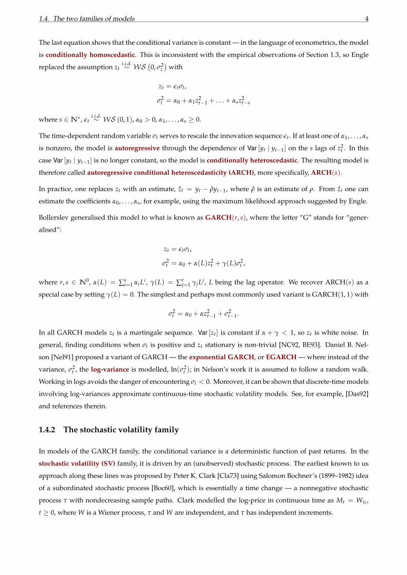
1.4. The two families of models 4
The last equation shows that the conditional variance is constant — in the language of econometrics, the model
is conditionally homoscedastic. This is inconsistent with the empirical observations of Section 1.3, so Engle
replaced the assumption zti.i.d.∼ WS
(0, σ2
z)
with
zt = εtσt,
σ2t = α0 + α1z2
t−1 + . . . + αsz2t−s
where s ∈N∗, εti.i.d.∼ WS (0, 1), α0 > 0, α1, . . . , αs ≥ 0.
The time-dependent random variable σt serves to rescale the innovation sequence εt. If at least one of α1, . . . , αs
is nonzero, the model is autoregressive through the dependence of Var [yt | yt−1] on the s lags of z2t . In this
case Var [yt | yt−1] is no longer constant, so the model is conditionally heteroscedastic. The resulting model is
therefore called autoregressive conditional heteroscedasticity (ARCH), more specifically, ARCH(s).
In practice, one replaces zt with an estimate, zt = yt − ρyt−1, where ρ is an estimate of ρ. From zt one can
estimate the coefficients α0, . . . , αs, for example, using the maximum likelihood approach suggested by Engle.
Bollerslev generalised this model to what is known as GARCH(r, s), where the letter “G” stands for “gener-
alised”:
zt = εtσt,
σ2t = α0 + α(L)z2
t + γ(L)σ2t ,
where r, s ∈ N0, α(L) = ∑si=1 αiLi, γ(L) = ∑r
j=1 γjLj, L being the lag operator. We recover ARCH(s) as a
special case by setting γ(L) = 0. The simplest and perhaps most commonly used variant is GARCH(1, 1) with
σ2t = α0 + αz2
t−1 + σ2t−1.
In all GARCH models zt is a martingale sequence. Var [zt] is constant if α + γ < 1, so zt is white noise. In
general, finding conditions when σt is positive and zt stationary is non-trivial [NC92, BE93]. Daniel B. Nel-
son [Nel91] proposed a variant of GARCH — the exponential GARCH, or EGARCH — where instead of the
variance, σ2t , the log-variance is modelled, ln(σ2
t ); in Nelson’s work it is assumed to follow a random walk.
Working in logs avoids the danger of encountering σt < 0. Moreover, it can be shown that discrete-time models
involving log-variances approximate continuous-time stochastic volatility models. See, for example, [Das92]
and references therein.
1.4.2 The stochastic volatility family
In models of the GARCH family, the conditional variance is a deterministic function of past returns. In the
stochastic volatility (SV) family, it is driven by an (unobserved) stochastic process. The earliest known to us
approach along these lines was proposed by Peter K. Clark [Cla73] using Salomon Bochner’s (1899–1982) idea
of a subordinated stochastic process [Boc60], which is essentially a time change — a nonnegative stochastic
process τ with nondecreasing sample paths. Clark modelled the log-price in continuous time as Mt = Wτt ,
t ≥ 0, where W is a Wiener process, τ and W are independent, and τ has independent increments.

1.4. The two families of models 5
Clark’s successors followed a somewhat different path — that of modelling volatility explicitly as a stochastic
process. As far as we know, the first papers to propose this approach were written by Stephen J. Taylor [Tay82]
and by George E. Tauchen and Mark Pitts [TP83], who all worked in discrete time. We shall use lower-case
letters to denote discrete-time stochastic processes in this chapter, so we replace Mt with mt in this instance.
Taylor modelled the daily (continuously compounded, or log-) returns, i.e. the differences in log-prices, yt :=
mt −mt−1, t ∈N∗, as
yt = εtext/2, (1.6)
xt+1 = µ(1− φ) + φxt + σvηt, (1.7)
where t ∈ N0, xt is the discrete-time stochastic process representing the log-variance of the log-returns (the
volatility, then, is σt := ext/2), µ is the mean log-variance, φ the persistence parameter, σv the volatility of
log-variance, ε0, ε1, . . . and η0, η1, . . . are all i.i.d. N (0, 1).6
As in EGARCH, working with logs, xt = ln(σ2t ), avoids the possibility of encountering a negative volatility σt.
It also enables the discrete-time model to approximate a continuous-time one [Das92]. On its own, (1.7) is an
AR(1) process — a natural discrete-time approximation of the continuous-time Ornstein–Uhlenbeck process.
When |φ| < 1, this process is strictly stationary with unconditional mean E [xt] = µ and variance Var [xt] =
σ2v /(1− φ2). The persistence parameter, φ, determines the rate of mean-reversion. The half-life of the AR(1)
process (1.7) is given by ln(0.5)/ ln(|φ|). It is the number of periods that the process needs, on average, to
halve its distance from the mean. Sometimes (1.7) is parameterised with α := µ(1− φ), as in [HRS94].
Others have modelled volatility (or various functions thereof) as continuous-time stochastic processes.
Herb Johnson pioneered this direction in a working paper published in 1979 [Joh79] and later continued this
work in collaboration with David Shanno [JS87]. Along these lines, James B. Wiggins [Wig87] studied the
model
dMt = κ dt + σt dW(M)t , M0 = ln s0,
dσt = f (σt) dt + σvσt dW(σ)t ,
where f is a deterministic function, W(M) and W(σ) are standard Wiener processes, and dW(M) dW(σ) = ρ dt,
so the log-price and volatility are possibly correlated (we will return to this correlation in Section 1.5). In the
much-studied model by John C. Hull and Alan White [HW87], the second SDE is replaced by
dσ2 = f (σt) σ2t dt + g(σt) σ2
t dW(σ)t ,
where g is a nonnegative deterministic function. f can be selected so that volatility, σt, (in the case of Wiggins)
or variance, σ2t , is the mean-reverting Ornstein–Uhlenbeck (OU) process and, indeed, both papers consider this
special case. Mean reversion is consistent with the empirically observed volatility clustering. Elias M. Stein
and Jeremy C. Stein also model volatility as an OU process [SS91]. Another popular model by Steven L. Hes-
ton [Hes93] is expressed in terms of variance: when σ follows an OU process, by Ito’s lemma, σ2 follows the
square-root (or CIR) process used by Cox, Ingersoll, and Ross [CIR85].

1.5. The statistical leverage effect 6
Many of the papers looking at stochastic volatility in continuous time have the pricing of options and other
derivatives as their primary concern. For example, [HW87, JS87, Wig87] use series expansions and/or numer-
ical methods to determine option prices; [SS91, Hes93] are also concerned with options. As in this dissertation
we are interested in econometrics rather than derivatives pricing, we shall not go into further details. Econo-
metricians prefer discrete-time models since they lend themselves more easily to forecasting and parameter
estimation.
1.5 The statistical leverage effect
One of the aspects of the volatility process highlighted in [BS73] is the relation between stock returns and
changes in volatility:
I have believed for a long time that stock returns are related to volatility changes. When stocks go
up, volatilities seem to go down; and when stocks go down, volatilities seem to go up. The extreme
example of this is the depression of the 30’s. Stocks went way down, and volatilities went way up.
The term statistical leverage effect (or simply leverage effect) refers to thus observed negative correlation
between changes in asset prices and changes in volatility. The reason for this name may not be immediately
apparent. The term leverage is synonymous with the debt-equity ratio of a company calculated by dividing
the company’s total liabilities by shareholders’ equity, indicating what portion of equity and debt the company
is using to finance its assets. The term takes its origin in the following explanation suggested by Black [BS73]:
A drop in the value of the firm will cause a negative return on its stock, and will usually increase
the leverage of the stock.7
Ibid. he observed that the volatility changes corresponding to stock returns were of too great a magnitude to
be explained by the leverage alone, suggesting that “other causal factors must be at work”. Other researchers
have expressed this view.8 The view is reinforced by an empirical study [HL11] of a sample of all-equity-
financed companies from January 1972 to December 2008, where the authors find that the leverage effect for
these companies is just as strong, if not stronger, than for debt-financed companies, concluding that “Black’s
leverage effect is not due to leverage”. Bearing in mind these reservations, we shall nonetheless refer to the
effect by its historical name.
1.6 A stochastic volatility model with leverage and jumps
Arguments have been heard in favour of both the GARCH [MT90] and stochastic volatility families of mod-
els [KSC98]. We have seen that the conditional variance is driven by a separate source of randomness in the
SV family, whereas in GARCH it is a deterministic function of past returns. The introduction of a separate
stochastic process to govern volatility is particularly appealing at higher frequencies, where that process can
be thought of as a representation of the information flow [PMD14, page 528]. The SV framework is also closely

1.6. A stochastic volatility model with leverage and jumps 7
linked to realised volatility measures [BNS02], which have been gaining importance in high-frequency econo-
metrics. It has also been shown [Das92] that the SV family of models offer better discrete-time approximations
to the continuous-time model used in [HW87]. We shall focus exclusively on SV in this work.
Andrew C. Harvey, Esther Ruiz, and Neil Shephard [HRS94] extended Taylor’s model [Tay82] mentioned in
Section 1.4.2 to include the leverage effect. Bjørn Eraker et al. formulated a similar model with jumps, but no
leverage [EJP03]. Michael K. Pitt, Sheheryar Malik, and Arnaud Doucet combine the two models to obtain a
new one — the stochastic volatility with leverage and jumps (SVLJ). They investigate this model in a series
of papers [MP09, MP11a, MP11b, PMD14]9. We shall use SVLJ as a basis for our discussion, so let us take a
closer look at it.
The model has the general form of Taylor’s (1.6) and (1.7) with two modifications. For t ∈ N0, let yt denote
the log-return on an asset and xt denote the log-variance of that return. Then
yt = εtext/2 + Jtvt, (1.8)
xt+1 = µ(1− φ) + φxt + σvηt, (1.9)
where, as before, µ is the mean log-variance, φ is the persistence parameter, σv is the volatility of log-variance10.
The first change to Taylor’s original model is the introduction of correlation between εt and ηt:(εtηt
)∼ N (0, Σ) , Σ =
(1 ρρ 1
).
The correlation ρ is the leverage parameter. As a consequence of the discussion in Section 1.5, we shall assume
ρ ∈ [−1, 0). The second change is the introduction of jumps in (1.8): Jt ∈ 0, 1 is a Bernoulli counter with
intensity p (thus p is the jump intensity parameter), vt ∼ N(
0, σ2J
)determines the jump size (thus σJ is the
jump volatility parameter).
We obtain a stochastic volatility with leverage (SVL), but no jumps, if we delete the Jtvt term or, equivalently,
set p to zero. Taylor’s original model is a special case of SVLJ with p = 0, ρ = 0. In Figure 1.1 we show an
example of the SVLJ data generated using the StateSpaceModelDataGenerator of BayesTSA.
Here we use the convention adopted in [HS96, KSC98, OCSN04, PMD14] and designate the disturbance that
propagates the log-variance between the times t and t + 1 by ηt. In much of the literature [HRS94, Rui94, Yu05]
this disturbance is designate ηt+1, so (1.9) becomes
xt+1 = µ(1− φ) + φxt + σvηt+1. (1.10)
In discrete-time econometric models the choice between (1.9) and (1.10) is a matter of convention. The im-
portant point to realise is that, whichever convention that we use, in this model, it is the disturbance on the
log-return yt and the disturbance that propagates the log-variance from xt to xt+1 that are correlated. If the
disturbance on the log-return yt were instead correlated with the disturbance that propagated the log-variance
from xt−1 to xt, we would have a different correlation structure and therefore a different model. Throughout
the literature, yt is the log-return that is related, through (1.8), to xt. In [Yu05], although the convention (1.10) is
used, (1.9) is described as “clearer and more consistent”. We shall stick with (1.9), so in our case Cor [εt, ηt] = ρ,

1.6. A stochastic volatility model with leverage and jumps 8
0 500 1000 1500 20002.01.51.00.50.00.51.01.52.02.5
log-variance
0 500 1000 1500 200002468
1012
variance
0 500 1000 1500 20000.00.51.01.52.02.53.03.5
volatility (standard deviation)
0 500 1000 1500 20001510
505
10152025
log-return
0 500 1000 1500 20004.44.64.85.05.25.45.65.86.06.2
log-price
0 500 1000 1500 2000time
50100150200250300350400450
price
Figure 1.1: An example of the SVLJ data generated using StateSpaceModelDataGenerator of the BayesTSAlibrary. Here we have used the same parameters as those in Figure 1 in [PMD14], namely µ = 0.25, φ = 0.975,σ2
v = 0.025, ρ = −0.8, p = 0.01, σ2J = 10. The vertical red lines indicate the times at which the simulated jumps
occur. We assume that the initial price is 100

1.7. Conclusions and further reading 9
xt−1 xt xt+1
yt−1 yt yt+1
εt−1 εt εt+1
ηt−1 ηt
(a)
xt−1 xt xt+1
yt−1 yt yt+1
εt−1 εt εt+1
ηt ηt+1
(b)
xt−1 xt xt+1
yt−1 yt yt+1
εt−1 εt εt+1
ηt−1 ηt
(c)
xt−1 xt xt+1
yt−1 yt yt+1
εt−1 εt εt+1
ηt ηt+1
(d)
Figure 1.2: The two conventions used in designating disturbances (noises) in econometric models and the twodifferent correlation structures between the disturbances. Within each subfigure we show the two disturbancesthat are assumed to be correlated in bold red; all the other disturbances are assumed to be uncorrelated. Sub-figures (a) and (c) show the first convention, where the disturbance that propagates xt to xt+1 is ascribed totime t and so referred to as ηt. Subfigures (b) and (d) show the second convention, where the disturbance thatpropagates xt to xt+1 is ascribed to time t + 1 and so referred to as ηt+1 Subfigures (a) and (b) show the firstcorrelation structure (CS1), in which the disturbance εt, involved in yt (yt being a function of xt and εt), iscorrelated with the disturbance that propagates xt to xt+1. Subfigures (c) and (d) show the second correlationstructure (CS2), in which the disturbance εt, involved in yt (yt being a function of xt and εt), is correlated withthe disturbance that propagates xt−1 to xt
the rest of the disturbances being independent. The differences between the two conventions used in the liter-
ature to designate the noises and the two different correlation structures are summarised in Figure 1.2.
Harvey and Shephard [HS96] propose a quasi-maximum likelihood (QML)11 approach to estimate the pa-
rameters of the SVL model. They start by squaring the log-returns and taking logs to obtain ln y2t = xt + ln ε2
t .
They then obtain a linear state-space representation of the problem and apply the Kálmán filter (see Chap-
ter 2). The likelihood obtained from an application of the Kálmán filter is then used in the QML procedure to
estimate the parameters of the model. Sangjoon Kim, Neil Shephard, and Siddhartha Chib [KSC98] and Re-
nate Meyer and Jun Yu [MY00] use Markov chain Monte Carlo (MCMC) techniques to estimate the parameters
of SVL. Eric Jacquier, Nicholas G. Polson and Peter E. Rossi [JPR04] apply MCMC to a different12 stochastic
volatility model with leverage. Particle filtering methods are applied to SVLJ by Pitt et al. [PMD14] and Da-
vide Raggi and Silvano Bordignon [RB06]. The latter incorporate an MCMC step to avoid degeneration of the
particles. Petar M. Djuric, Mahsiul Khan, and Douglas E. Johnston apply particle filters to SVL and employ
Rao-Blackwellisation of the unknown static parameters.
1.7 Conclusions and further reading
We refer the reader to [GHR96, She96, She05] for more thorough reviews of SV models. A summary of the
modelling approaches can also be found in [Gat06, Chapter 1]. A more nuanced guided tour of the history of
the subject is contained in [Hau08].

1.7. Conclusions and further reading 10
In the next chapter we shall examine the algorithmic toolkit of stochastic filtering and, in Section 2.4, show how
it has been applied to SVLJ. We shall also introduce some fundamentals of MCMC. In the ensuing chapters
we shall apply both filtering and MCMC to various stochastic volatility models and build on the theoretical
foundation reviewed in the first two chapters.

Chapter 2
The filtering framework
2.1 Introduction
In this chapter we shall present the foundations of stochastic filtering from the standpoint of an elec-
tronic trading practitioner. Let’s start in full generality. The totally ordered set T will represent the time.
Let(Ω,F , P, (Ft)t∈T
)be a filtered probability space satisfying the usual conditions. An (Ft)t∈T-adapted
stochastic process X = (Xt)t∈T, taking values on a complete separable metric space S, will represent the (hid-
den, latent, unobserved) state of the system at time t. We shall refer to X as the state process and to S as the
state space. While we cannot observe X directly, we have access to another (Ft)t∈T-adapted stochastic pro-
cess Y = (Yt)t∈T, which is a function of X and a Wiener process V = (Vt)t∈T: Yt := ht(Xt, Vt), t ∈ T. The
function ht is sometimes referred to as the observation model13. The specification of the dynamics of X, often
in the form of an SDE, is called the process model.
Let (Yt)t∈T be the σ-algebra generated by the observation process Y. The filtering problem consists of
computing the filtering distribution, π = (πt)t∈T, the conditional distribution of Xt given (Yt)t∈T. It
is defined as a random probability measure, which is — crucially — measurable w.r.t. (Yt)t∈T, such that
E [ψ(Xt) | Yt] =∫
Sψ(x)πt(dx) for all statistics ψ for which both sides of the above identity make sense. A
formal definition of π relies on some technicalities and can be found in [BC09, Chapter 2].
Interest in the filtering problem dates back to the late 1930s – early 1940s. It was considered in Andrey Nikolae-
vich Kolmogorov’s (1903–1987) work on time series [Kol33, Kol41, Kol56] and Norbert Wiener’s (1894–1964)
on improving radar communication during WWII [Wie49]14, which first appeared in 1942 as a classified mem-
orandum nicknamed ‘The Yellow Peril’ [Wie42], so named after the colour of the paper on which it was printed
[BC09]. In [Wie42, Wie49], Wiener considered the special case of a stationary state process and additive noise
and minimised the mean square error between the estimated and actual state process, working in continuous
time. The result is nowadays known as the Wiener filter. A discrete-time equivalent of this filter was obtained
independently by Kolmogorov and published in earlier in Russian [Kol41]. Due to the contributions by these
two scientists, the theory is referred to as the Wiener–Kolmogorov theory of filtering and prediction [KB61].
Rudolf Emil Kálmán (1930–2016) extended this work to non-stationary processes. This work had military
applications, notably the prediction of ballistic missile trajectories. Non-stationary processes were required
11

2.1. Introduction 12
to realistically model their launch and re-entry phases. Of course, non-stationary processes abound in other
fields — even the standard Brownian motion of the basic Bachelier model [Bac00] in finance is non-stationary.
Kálmán’s fellow electrical engineers initially met his ideas with skepticism, so he ended up publishing in a
mechanical engineering journal [Kál60a]. In 1960, Kálmán visited the NASA Ames Research Center, where
Stanley F. Schmidt took interest in this work. This led to its adoption by the Apollo programme and other
projects in aerospace and defence.
The discrete-time version of the filter derived in [Kál60a] is now known as the Kálmán filter (KF).
The continuous-time version, known as the Kálmán–Bucy filter15, was published in a joint paper with
Richard Snowden Bucy (b. 1935) [KB61]. Before meeting Kálmán, Bucy worked on continuous-time stochastic
filtering independently, with James Follin, A. G. Carlton, and James Hanson at John Hopkins Applied Physics
Lab in the late 1950s. The Kálmán and Kálmán–Bucy filters address the particularly important special case
when the process model and the observation model are linear and both stochastic processes are Gaussian,
the so-called linear-Gaussian case16, where there is an analytic solution for π. The general case of the filter-
ing problem was addressed by Ruslan Leontyevich Stratonovich (1930–1997) [Str59, Str60], Harold J. Kushner
(b. 1933) [Kus67], and Moshe Zakai (1926–2015) [Zak69].
The general solutions are, however, infinite-dimensional and not easily applicable. In practice, numerical
approximations are employed. Particle filters constitute a particularly important class of such approxima-
tions. These methods are sometimes referred to as sequential Monte Carlo (SMC), a term coined by Liu and
Chen [LC98]. The Monte Carlo techniques requisite for particle filtering date back to the work of Hammersley
and Morton [HM54]. Sequential importance sampling (SIS) dates back to the work of Mayne and Hand-
schin [May66, HM69]. The important resampling step was added by Gordon, Salmond, and Smith [GSS93],
based on an idea by Rubin [Rub87], to obtain the first sequential importance resampling (SIR) filter, which, in
our experience, remains the most popular particle filtering algorithm used in practice. Other important early
contributions to the development of particle filtering include [Kit93, Kit96, BBGL97, IB98, LC98, HK98, CCF99].
Our overview of the development of stochastic filtering theory is necessarily brief. We focus on the de-
velopment of the algorithms to motivate the discussion in the sequel, and merely scratch the surface
of advances in stochastic analysis on which these algorithms rely. The reader interested in this im-
portant aspect of the theory can examine the work of Robert Horton Cameron (1908–1989), Masatoshi
Fujisaki, Igor Vladimirovich Girsanov (1934–1967), Gopinath Kallianpur (1925–2015), Hiroshi Kunita (b.
1937), Robert Shevilevich Liptser (b. 1936), William Theodore Martin (1911–2004), Albert Nikolaevich
Shiryaev (b. 1934), Charlotte Striebel (1929–2014), including the significance of the Cameron-Martin-Girsanov
theorem [CM44, Gir60], the Fujisaki–Kallianpur–Kunita equation and orthogonal projection in Hilbert
spaces [FKK72], the Kallianpur–Striebel formula [KS69b, KS69a, Kal80, LS92], and non-linear filtering of
Markov diffusion processes and jump processes [Shi66, LS68].

2.2. Special case: general state-space models 13
2.2 Special case: general state-space models
We have spoken thus far in considerable generality. Let us turn our attention to a particularly important
special case of the filtering problem, viz. filtering for discrete-time, general state-space models, also known as
hidden Markov models (HMM) [LB13]. Such models are prevalent in econometrics due to the relative ease
of the estimation of their parameters and forecasting. We shall keep our notation and terminology roughly
consistent with [CM14, Section 2.2].
These models are discrete-time, i.e. we regard T as a countable set. Without loss of generality, we shall identify
T with N0. Since our models consider the evolution of a system over time, they are described as dynamic. We
shall also assume that the state process (X t)t∈T takes values in the Euclidean space S = RdX , dX ∈N∗ (so it is
now represented by a state vector), the observation process (Y t)t∈T\0 takes values in the Euclidean space RdY ,
dY ∈N∗ (so it is now represented by an observation vector).
We assume that the sequence of random variables X0, X1, X2, . . . is a Markov chain17 — i.e., the conditional
distribution of X t, t ∈ N∗, given X0, . . . , X t−1, depends only upon X t−1. Mathematically this means that, for
each A ∈ BRdX :
P [X t ∈ A | X0 = x0, . . . , X t−1 = xt−1] = P [X t ∈ A | X t−1 = xt−1] =: τt(A | xt−1),
where τt : BRdX ×RdX → [0, 1] is referred to as the Markov transition kernel. The state process (X t)t∈T is
assumed to be not directly observable, hence the term ‘latent Markov model’.
We regard the sequence of random variables Y1, Y2, . . . as observations ordered in time — such a sequence is
usually referred to as a time series. Each random variable Y t will be assumed to be conditionally independent
of other observations given the state X t, i.e., for t ∈N∗,
P[Y t ∈ A | X0 = x0, . . . , X t = xt, (Y s = ys)s∈N∗ ,s,t
]= P [Y t ∈ A | X t = xt]
for each A ∈ BRdY .
For all t ∈ N∗, A ∈ BRdY , the probability measure γt(A | xt) := P [Y t ∈ A | X t = xt] is assumed to have a
positive density, denoted pγt(y | x) and called the observation density, w.r.t. the Lebesgue measure, hence
γt(A | xt) =∫
A pγt(y | xt) dy. While X t is indeed latent, it is related to the observation Y t via pγt .
2.3 Particle filtering methods
Particle filtering methods rely on the numerical approximation of πt with a set of ‘particles’. To apply these
methods we don’t require the Markov transition kernel to have a probability density (the Markov transition
density), i.e. for all t ∈ N∗, A ∈ BRdX , pτt in τt(A | xt−1) =∫
A pτt(x | xt−1) dx. However, we need to be able
to sample from the Markov transition kernel.

2.3. Particle filtering methods 14
Algorithm 2.1 Particle filter: sequential importance resampling (SIR)1. Initialisation step: At time t = 0, draw M i.i.d. samples (called particles) from the initial distribution
τ0 = π0. Also, initialise M normalised (to 1) weights to an identical value of 1M . For i = 1, 2, . . . , M, the
samples will be denoted x(i)0 | 0 and the normalised weights λ(i)0 .
2. Recursive step: At time t ∈N∗, let(
x(i)t−1 | t−1
)i=1,...,M
be the particles generated at time t− 1.
(a) Importance sampling:
i. For i = 1, . . . , M, sample x(i)t | t−1 from the Markov transition kernel τt(· | x(i)t−1 | t−1).
ii. For i = 1, . . . , M, use the observation density to compute the non-normalised weights
ω(i)t := λ
(i)t−1 · pγt(yt | x(i)t | t−1) (2.1)
and the values of the normalised weights before resampling (‘br’), brλ(i)t := ω
(i)t / ∑M
k=1 ω(k)t .
(b) Resampling (or selection): For i = 1, . . . , M, use an appropriate resampling algorithm (such asAlgorithm 2.2) to sample x(i)t | t from the mixture
M
∑k=1
brλ(k)t δ(xt − x(k)t | t−1), (2.2)
where δ(·) denotes the Dirac delta generalised function, and set the normalised weights after re-sampling, λ
(i)t , appropriately (for most common resampling algorithms this means λ
(i)t := 1
M ).
Here we have given the most common version of the particle filter known as the sequential importance resam-
pling (SIR)18 algorithm [GSS93, Rub87]. There are many variations on Algorithm 2.1. For example, in some
such variations the number of particles M may vary with time, so instead of M we would have an appropri-
ately defined Mt [LXhSqWt10]. In this particular formulation of the filter, all the weights after resampling are
set to 1M , so we could write (2.1) as ω
(i)t := pγt(yt | x(i)t | t−1), i = 1, . . . , M, and omit the initialisation of the
normalised weights at time 0, λ(i)0 , since they wouldn’t be used. This isn’t the case in all variants of the particle
filter. A simpler version of the filter would omit the resampling step altogether; instead, for i = 1, . . . , M,
setting λ(i)t := brλ
(i)t and x(i)t | t := x(i)t | t−1. This version of the algorithm, known as sequential importance
sampling (SIS) [May66, HM69], suffers from the degeneracy problem [LC98], [CMR05, Chapter 7] when, in
some situations, only a few particles end up with significant weight, and all the other particles have near-zero
weights. The resampling step is designed to remedy this. The particular scheme that we give here as Algo-
rithm 2.2 is known as multinomial resampling [Rub87, GSS93, ET94]19 and the filter that uses it is sometimes
referred to as the (weighted) bootstrap filter. The naïve implementation of multinomial resampling step has
the time complexity O (M ln M). An implementation based on [CCF99] has the time complexity O (M). One
alternative is to use stratified sampling [Kit96, LC98, CCF99], which won’t be discussed here. It introduces no
computational overhead.

2.4. Applying the particle filter to the stochastic volatility model with leverage and jumps 15
Algorithm 2.2 Multinomial resampling
Notice that we are working with the normalised weights computed before resampling, brλ(1)t , brλ
(2)t , . . . , brλ
(M)t .
1. For i = 1, 2, . . . , M, compute the cumulative sums brΛ(i)t = ∑i
k=1brλ
(k)t , so that, by construction, Λ(M)
t =1.
2. Generate M random samples from U (0, 1), u1, u2, . . . , uM.
3. For each i = 1, . . . , M, choose the particle x(i)t | t := x(j)t | t−1 with j ∈ 1, 2, . . . , M− 1 such that ui ∈[
brΛ(j)t , brΛ(j+1)
t
].
Thus we end up with M new particles (children), x(1)t | t, . . . , x(M)t | t sampled from the existing set
x(1)t | t−1, . . . , x(M)t | t−1, so that some of the existing particles may disappear, while others may appear multiple
times. For each i = 1, . . . , M the number of times x(i)t | t−1 appears in the resampled set of particles is known as
that particle’s replication factor, N(i)t . Set the normalised weights after resampling: λ
(i)t := 1
M . We could view
this algorithm as the sampling of the replication factors N(1)t , . . . , N(M)
t from the multinomial distribution with
probabilities brλ(1)t , . . . , brλ
(M)t , respectively. Hence the name of the method.
For each t ∈N∗, this algorithm provides the prior and posterior, respectively, approximations to πt:
πMt | t−1 :=
M
∑i=1
λ(i)t−1δ(xt − x(i)t | t−1), πM
t | t :=M
∑i=1
λ(i)t δ(xt − x(i)t | t)
(when using the resampling scheme given here the resampled weights are all set to 1M , so this constant can
be factored out of the sum). The prior state mean and covariance estimates in the particle filter are given by,
respectively,
xt | t−1 :=M
∑i=1
λ(i)t−1 x(i)t | t−1, Pt | t−1 :=
M
∑i=1
λ(i)t−1(x(i)t | t−1 − xt | t−1)
ᵀ(x(i)t | t−1 − xt | t−1).
Similarly, one obtains the posterior state mean and covariance before resampling, br xt | t and brPt | t, (using
the the weights brλ(i)t and particles x(i)t | t−1) and after resampling, xt | t and Pt | t, (using the weights λ
(i)t and
particles x(i)t | t).
2.4 Applying the particle filter to the stochastic volatility model withleverage and jumps
Michael K. Pitt, Sheheryar Malik, and Arnaud Doucet apply the particle filter to the SVLJ model of Sec-
tion 1.6 [MP09, MP11a, MP11b, PMD14]20. From the filtering perspective, the latent, unobserved log-variance
is the state and the log-return, which is observable on the markets, the observation. Using the fact that the
disturbances in (1.8) and (1.9) are conditionally Gaussian, they write
ηt = ρεt +√
1− ρ2ξt (2.3)
where ξti.i.d.∼ N (0, 1), turning (1.9) into
xt = µ(1− φ) + φxt−1 + σvρεt−1 + σv
√1− ρ2ξt−1. (2.4)

2.4. Applying the particle filter to the stochastic volatility model with leverage and jumps 16
In the absence of jumps, εt = yte−xt/2, and (2.4) can be further rewritten as
xt = µ(1− φ) + φxt−1 + σvρyt−1e−xt−1/2 + σv
√1− ρ2ξt−1.
Even in the absence of jumps p(xt | xt−1, yt−1) is highly nonlinear, so particle methods are prime candidates
for devising a filtering scheme.
Notice that
p(εt | xt, yt) = δ(yte−xt/2)P [Jt = 0 | xt, yt] + ϕ(
εt; µεt | Jt=1, σ2ε | Jt=1
)P [Jt = 1 | xt, yt] .
Pitt et al. design a procedure for simulating εt from the mixture density p(εt | xt, yt), which is then used in 2.4
to propagate the state. It is described in detail in Appendix B of [MP09]; we have implemented it in BayesTSA.
In the same Appendix they derive the values of the conditional moments µεt | Jt=1 and σ2ε | Jt=1.
The initial distribution of x0 is taken to be N(0, σ2
v /(1− φ2)). This, then, leads to the following modification
of Algorithm 2.1 for this special case with nonadditive, correlated noises:
Algorithm 2.3 An adaptation of the particle filter (Algorithm 2.1) developed by Pitt et al. for the SVLJ model
1. Initialisation step: At time t = 0, draw M i.i.d. particles from the initial distributionN(0, σ2
v /(1− φ2)).
Also, initialise M normalised (to 1) weights to an identical value of 1M . For i = 1, 2, . . . , M, the samples
will be denoted x(i)0 | 0 and the normalised weights λ(i)0 .
2. Recursive step: At time t ∈N∗, let(
x(i)t−1 | t−1
)i=1,...,M
be the particles generated at time t− 1.
(a) Importance sampling:
i. A. For i = 1, . . . , M, sample ε(i)t−1 from p(εt−1 | xt−1 = x(i)t−1 | t−1, yt−1). (If no yt−1 is available,
as at t = 1, sample from p(εt−1 | xt−1 = x(i)t−1 | t−1)).
B. For i = 1, . . . , M, sample x(i)t | t−1 from p(xt | xt−1 = x(i)t−1 | t−1, yt−1, ε(i)t−1).
ii. For i = 1, . . . , M, compute the non-normalised weights
ω(i)t := λ
(i)t−1 · pγt(yt | x(i)t | t−1), (2.5)
using the observation density
p(yt | x(i)t | t−1, p, σ2J ) = (1− p)
[(2πex(i)t | t−1
)−1/2
exp(−y2
t /(2ex(i)t | t−1)
)]+
p
[(2πex(i)t | t−1 + σ2
J
)−1/2
exp(−y2
t /(2ex(i)t | t−1 + σ2J )
)],
and the values of the normalised weights before resampling (‘br’): brλ(i)t := ω
(i)t / ∑M
k=1 ω(k)t .
(b) Resampling (or selection): For i = 1, . . . , M, use an appropriate resampling algorithm (such asAlgorithm 2.2) sample x(i)t | t from the mixture ∑M
k=1brλ
(k)t δ(xt− x(k)t | t−1), where δ(·) denotes the Dirac
delta generalised function, and set the normalised weights after resampling, λ(i)t , according to the
resampling algorithm.
The result of applying this algorithm to simulated data is shown in Figure 2.1.

2.4. Applying the particle filter to the stochastic volatility model with leverage and jumps 17
0 500 1000 1500 20002.01.51.00.50.00.51.01.52.02.5
state
posterior filtered state
true state
0 500 1000 1500 20001.51.00.50.00.51.01.5
error
0 500 1000 1500 20000.20
0.25
0.30
0.35
0.40rmse
0 500 1000 1500 20000.1
0.2
0.3
0.4
0.5
0.6posterior filtered state standard deviation
0 500 1000 1500 20001510
505
10152025
observation
true observation
predicted observation
0 500 1000 1500 2000201510
505
10152025
innovation
innovation
15 10 5 0 5 10 15 201510
505
101520
standardised innovation Q-Q plot
0 500 1000 1500 20000.50.00.51.01.52.02.5
CUSUM
0 500 1000 1500 2000350030002500200015001000
5000
loglikelihood
0 500 1000 1500 2000
time
250300350400450500550600
effective sample size
Figure 2.1: The result of applying Algorithm 5.1 to the SVLJ data generated usingStateSpaceModelDataGenerator of the BayesTSA library. Here we have used the same parameters asthose in Figure 1 in [PMD14], namely µ = 0.25, φ = 0.975, σ2
v = 0.025, ρ = −0.8, p = 0.01, σ2J = 10. We assume
that the parameters are known exactly, i.e. we use the same parameters in the particle filter as the ones thatwe used to generate the data. The figure includes the diagnostic plots produced by BayesTSA. The tails on theQ-Q plot deviate from normal significantly due to the substantial jumps (σ2
J = 10)

2.5. The Kálmán filter 18
2.5 The Kálmán filter
The model considered in Section 2.4 is nonlinear with correlated Gaussian state process noise and observation
noise. Let us now consider a simpler and particularly important specialisation of the general state-space model
of Section 2.2 — the linear-Gaussian state-space model. For t ∈ N∗, suppose that our dX-dimensional state
vector is driven by dW-dimensional noise and evolves according to the process model that is specified by the
single equation — the process (evolution, transition) equation
X t = FtX t−1 + at + W twt, (2.6)
and our dY-dimensional observation vector, incorporating dV-dimensional observation noise, is related to the
state by the observation model (or, in this case, the observation equation)
Y t = HtX t + bt + V tvt, (2.7)
where Ft ∈ RdX×dX , W t ∈ RdX×dW , at ∈ RdX ; whereas wt ∼ N (0, Qt) are RdW -valued random variables;
Ht ∈ RdY×dX , V t ∈ RdY×dV , bt ∈ RdY ; whereas vt ∼ N (0, Rt) are RdV -valued random variables. We assume
that X0 ∼ N(
x0 | 0, P0 | 0
)and the random variables X0, w1, . . . , wt, v1, . . . , vt are mutually independent.
The matrices Ft, at, W t, Qt, Ht, bt, V t, Rt are sometimes referred to as system matrices. When they don’t
depend on t, i.e., for all t, Ft = F fixed, etc., the system is called time invariant.
We could, equivalently, write (2.6) and (2.7), respectively, as
X t | X t−1 ∼ N(
FtX t−1 + at, W tQtWᵀt)
, Y t | X t ∼ N(
HtX t + bt, V tRtVᵀt)
,
or say that
pτt = ϕ(
FtX t−1 + at, W tQtWᵀt)
, pγt = ϕ(
HtX t + bt, V tRtVᵀt)
.
The Kálmán filter (Algorithm 2.4) [Kál60a, KB61] is an analytic solution to the filtering problem in this setting.
Algorithm 2.4 Kálmán filterFor each t ∈N∗, repeat the following two steps:
1. Prediction step:
(a) Predicted (prior) state estimate: xt | t−1 = Ft xt−1 | t−1 + at.
(b) Predicted (prior) error covariance: Pt | t−1 = FtPt−1 | t−1Fᵀt + W tQtWᵀt .
2. Update (or correction) step:
(a) Predicted observation: yt | t−1 = Ht xt | t−1 + bt.
(b) Innovation (or observation residual): yt = yt − yt | t−1.
(c) Innovation covariance: St = HtPt | t−1Hᵀt + V tRtVᵀt .
(d) (Optimal) Kálmán gain: Kt = Pt | t−1Hᵀt S−1t .
(e) Updated (posterior) state estimate: xt | t = xt | t−1 + Ktyt.
(f) Updated (posterior) error covariance: Pt | t = (I − KtHt)Pt | t−1.

2.6. Some examples of linear-Gaussian state space models 19
Proposition 2.5.1 (Some properties of the Kálmán filter). 1. Pt | t−1 is a faithful representation of the prior error
covariance: Pt | t−1 = Cov[
xt | t−1 − X t
];
2. Pt | t is a faithful representation of the posterior error covariance: Pt | t = Cov[
xt | t − X t
];
3. St is a faithful representation of the innovation covariance: St = Cov [yt];
4. the prior state estimate is unbiased: E[
xt | t−1 − X t
]= 0;
5. the posterior state estimate is unbiased: E[
xt | t − X t
]= 0;
6. The solution to the filtering problem at time t, xt | t, is:
(a) causal (or based on the observations): the estimate is obtained using only the observations ys for s ≤ t;
(b) optimal: xt | t minimises the mean square error (MSE), E
[∥∥∥X t − xt | t
∥∥∥2
2
], so it is a minimum mean
square error estimate (MMSE);
(c) online: for an arbitrary time t ∈ T, the estimate is available (prior, if we haven’t seen the observation yet,
otherwise posterior).
The iterative equation for the predicted (prior) error covariance,
Pt | t−1 = Ft(Pt−1 | t−2 − KtHtPt−1 | t−2)Fᵀt + W tQtWᵀt (2.8)
is a discrete-time, time-varying matrix Riccati equation. From this equation we notice21 that the covariance
calculations are independent of the state estimate calculations occurring elsewhere in the filter. Therefore it
is possible to perform the covariance calculations separately, offline. There is a rich mathematical theory of
matrix Riccati equations, which underly much of filtering and control [AKFIJ03]. In particular, it is known
that (2.8) converges to a steady state covariance, P∞, provided that the system is observable, a term coined
by Kálmán [Kál60b, Kál63], which means, informally, that the state of the system can be determined from the
observations.
From (2.8) we notice that the covariance calculations are independent of the state calculations, so can be per-
formed offline, i.e. before the filter is applied to observations arriving in real time.
It is worth noting here that Kálmán’s original thinking [Kál60a] wasn’t formally Bayesian. It was Y. C. Ho and
R. C. K. Lee [HL64] that would later reinterpret this filter from the Bayesian perspective. There are several
Bayesian ways to derive the Kálmán filter [BBM95]. For an overview of the filtering theory from the point of
view of a Bayesian, see [Che03].
2.6 Some examples of linear-Gaussian state space models
We shall now examine some situations where we get Kálmán-style, i.e. linear-Gaussian, state-space models of
the kind considered in Section 2.5. Before we turn to financial applications of Kálmán filtering, let us consider a
more basic and paradigmatic example from mechanics — the classical Newtonian system [Sim06, Example 5.1].

2.6. Some examples of linear-Gaussian state space models 20
2.6.1 A non-financial example: the Newtonian system
For simplicity, we shall disregard the process noise. Let r be the position of a particle, v its velocity, and a its
(constant) acceleration. Then dr/dtdv/dtda/dt
=
0 1 00 0 10 0 0
rva
.
The state of our system is given by the vector X t = (r, v, a)ᵀ. Denote the matrix of ones and zeros above by A.
Then the evolution of the state is described by the matrix differential equation dX tdt = AXt. By analogy with the
scalar ordinary differential equation, its solution is X t = eAtx0, where X t = (rt, vt, at)ᵀ is the state of the system
at time t and the matrix exponential is defined by the (matrix) Taylor series expansion eAt := ∑∞j=0
(At)j
j! . Note
that, for s ≤ t ∈ T, Xt = eA(t−s)Xs. Let us now discretise this equation using hk := t− s as the time interval
between the time ticks k− 1 and k (for k ∈N∗). We get Xk = FkXk−1, where
Fk := eAhk =∞
∑j=0
(Ahk)j
j!=
1 0 00 1 00 0 1
+
0 1 00 0 10 0 0
hk +12
0 0 10 0 00 0 0
h2k
=
1 hk h2k/2
0 1 hk0 0 1
,
since all the powers of A greater than 2 are zero matrices. We observe that this process model fits the Kálmán
filter paradigm, a hint as to why this paradigm is so widely applicable in practice.
2.6.2 Autoregressive moving average models
Consider the ubiquitous autoregressive moving average ARMA(p, q) model, which is often fitted to financial
time series:
yt = φ1yt−1 + . . . + φpyt−p + ηt + θ1ηt−1 + . . . + θqηt−q,
where ηt ∼ N(0, σ2). This model includes as special cases all AR(p) and MA(q) models. We account for the
possibility that the model is nonstationary (an autoregressive integrated moving average, ARIMA). There are
several ways of representing this model as a linear-Gaussian state-space model with a view to applying the
Kálmán filter. The approach that we give here is by far the most common [BD87, Har89, BJR94, Ham94b]. The
earlier approach by J. G. Pearlman [Pea80], while more efficient, would require one to deal with correlated
process and observation noises. Set m := max(p, q + 1), φi := 0 for i > p, θi := 0 for i > q. Then we get (2.6)
and (2.7) with dX = m, dY = 1, dW = 1, and no observation noise, and
X t =
yt
φ2yt−1 + . . . + φpyt−m+1 + θ1ηt + . . . + θm−1ηt−m+2φ3yt−1 + . . . + φpyt−m+2 + θ2ηt + . . . + θm−1ηt−m+3
...φmyt−1 + θm−1ηt
∈ Rm×1,
F =
φ1 1 0 · · · 0φ2 0 1 0...
.... . . . . .
...φm−1 0 0 1
φm 0 0 · · · 0
∈ Rm×m,

2.6. Some examples of linear-Gaussian state space models 21
0 20 40 60 80 100time
1.0
0.5
0.0
0.5
1.0true state
noisy observation
Figure 2.2: An ARMA(2, 1) time series generated using StateSpaceModelDataGenerator of the BayesTSAlibrary. Its parameters are φ1 = 0.75, φ2 = −0.4, θ1 = 0.7, and σ2 = 0.1. We have also generated noisyobservations of this series by adding to it white Gaussian noise with variance σ2/2
W =(1 θ1 · · · θm−1
)ᵀ ∈ Rm×1,
wt = ηt, Qt = σ2, H =(1 0 . . . 0
)∈ 1×m, bt = 0, Vt = 0.
If yt is stationary, then X t ∼ N (0, P) with P given by the equation P = FPFᵀ + σ2WWᵀ, so we can set the
initial state and error covariance to 0 and P, respectively. For a detailed discussion of applying the Kálmán
filter in this particular case, see [dJP00, ZW06].
2.6.3 Continuous-time stochastic processes: the Wiener process, geometric Brownianmotion, and the Ornstein–Uhlenbeck process
Let us now consider how we can construct state-space models by discretising some continuous-time stochastic
processes that are of particular importance in finance [PH06, Chapter 4], [Shr04, Chapter 3]. We begin with the
one-dimensional variance-scaled Wiener process with drift µ and volatility σ, given by the SDE
dXt = µ dt + σ dWt,
Let us now discretise the solution of this SDE, for s ≤ t ∈ T,
Xt = Xs + µ(t− s) + σ(Wt −Ws).
by setting hk := t− s as the time interval between the time ticks k− 1 and k (k ∈N∗) to obtain a special case of
the linear-Gaussian state-space model of Section 2.5,
Xk = FkXk−1 + ak + wk, (2.9)
where Fk = 1, ak = µhk, wk ∼ N(0, σ2hk
). It is not necessary to make the continuous time intervals, corre-
sponding to each discrete time tick, equal. We must, however, be careful, to scale the drift and process noise
variance appropriately, as they are functions of the time step hk.

2.6. Some examples of linear-Gaussian state space models 22
0 20 40 60 80 1001.0
0.5
0.0
0.5
1.0state
posterior filtered state
true state
0 20 40 60 80 1000.6
0.4
0.2
0.0
0.2
0.4
0.6
0.8error
0 20 40 60 80 1000.20
0.22
0.24
0.26
0.28
0.30
0.32
0.34
0.36
0.38rmse
0 20 40 60 80 1000.8
0.6
0.4
0.2
0.0
0.2
0.4
0.6observation
true observation
predicted observation
0 20 40 60 80 100
time
1.5
1.0
0.5
0.0
0.5
1.0innovation
innovation
Figure 2.3: The result of applying the Kálmán filter (Algorithm 2.4) to the noisy observation in Figure 2.2 usingthe state-space model of Section 2.6.2 plus additive observation noise with true parameters taken as known

2.6. Some examples of linear-Gaussian state space models 23
To handle the case of geometric Brownian motion (GBM) with percentage drift µ′ and percentage volatility
σ′,
dSt = µ′St dt + σ′St dWt,
we transform the process by taking the natural logarithm, Xt := ln St, obtaining the Wiener process with the
initial value X0 = ln S0, drift µ = µ′ − (σ′)2/2, and volatility σ′. We can then apply the Kálmán filter to the
transformed process.
Now consider the one-dimensional Ornstein–Uhlenbeck (OU) process [PH06, Chapter 4], the stationary
Gauss–Markov process given by the SDE
dXt = θ(µ− Xt) dt + σ dWt,
where Xt ∈ R, X0 = x0, and θ > 0, µ and σ > 0 are constants. The solution to this SDE is well-known:
Xt = x0e−θt + µ(1− e−θt) +∫ t
0σe−θ(t−u) dWu.
An Ito integral,∫ t
s f (u) dWu, of a deterministic integrand, f (u), is a Gaussian random variable with mean 0
and variance∫ t
0 f 2(u) du. In our case, f (u) = σe−θ(t−u), and∫ t
0 f 2(u) du = σ2
2θ
(1− e−2θt). Since this Markov
process is homogeneous, its transition density depends only upon the time difference. Setting, for s ≤ t ∈ T,
hk := t− s as the time interval between the time ticks k − 1 and k (for k ∈ N∗), we again get the discretised
process model equation (2.9), this time with Fk = e−θhk , ak = µ(1 − e−θhk ), wk ∼ N(
0, σ2
2θ
(1− e−2θhk
)).
Again, we observe that this process model fits the Kálmán filter paradigm.
These results readily extend to higher dimensions. The d-dimensional correlated Wiener process with drift
follows the SDE
dX t = µ dt + L dW t,
where the drift (or infinitesimal mean) µ is a d-dimensional real column vector, L is a (d× k)-dimensional real
matrix LLᵀ = Σ ∈ Rd×d is positive-definite, and W is a k-dimensional standard Wiener process. The matrix Σ
is referred to as the infinitesimal covariance matrix. Discretising with the timestep hk := t− s, as above, we
get the linear-Gaussian state-space model representation
Xk = FkXk−1 + ak + wk, (2.10)
where Fk = Id×d, ak = hkµ, wk ∼ N (0d×d, hkΣ).
The SDE for the d-dimensional version of the OU process [Meu10],
dX t = −Θ(X t − µ) dt + L dW t,
where Θ ∈ Rd×d, has the solution
X t = e−Θtx0 + (I − e−Θt)µ +∫ t
0eΘ(s−t)L dW s.
Hence, for s ≤ t ∈ T,
E[X t] = E
[e−Θtx0 + (I − e−Θt)µ +
∫ t
0eΘ(s−t)L dW s
]= e−Θtx0 + (I − e−Θt)µ,

2.7. The extended Kálmán filter 24
Cov(Xs, X t) = E
[(∫ s
0eΘ(u−s)L dWu
)(∫ t
0eΘ(v−t)L dWv
)T]
,
Var(Xt) = E
[(∫ s
0eΘ(u−t)L dWu
)(∫ s
0eΘ(u−t)L dWu
)T]
Itô isometry=
∫ t
0eΘ(u−t)ΣeΘT(u−t) du.
Meucci [Meu10], citing his correspondence with Van der Werf, shows how to compute this integral using
tensor calculus, obtaining
vec(Var(X t)) = (Θ⊕Θ)−1(
I − e−(Θ⊕Θ)t)
vec(Σ),
whence Var(X t) is obtained simply by ‘unstacking’ the columns of vec(Var(X t)). Hence we again obtain the
discretisation (2.10) using, as in the one-dimensional case, the fact that this Markov process is homogeneous.
The OU process is ubiquitous in finance and has applications in statistical arbitrage and cointegration [Meu10].
In practice, care is needed when implementing numerics dealing with the matrix exponentials that result
[ML03].
2.7 The extended Kálmán filter
We have now seen the two main algorithms of stochastic filtering: the particle filter of Section 2.3 and the
Kálmán filter of Section 2.5. Since the invention of these two algorithms, researchers have come up with
numerous new algorithms. Many of these algorithms fall into two categories: extensions of the particle filter
and extensions of the Kálmán filter. The scope of this work does not permit us to consider many of these
algorithms. In the sequel we shall consider only two important extensions of the Kálmán filter — the extended
Kálmán filter and the Gaussian assumed density filter.
We begin with the extended Kálmán filter (EKF). For t ∈ N∗, suppose that, instead of being given by equa-
tions (2.6) and (2.7), our process and observation models are, respectively,
X t = f t(X t−1, wt), Y t = ht(X t, vt),
where
f t : RdX ×RdW → RdX , f t : X, w 7→ f t(X, w),
ht : RdX ×RdV → RdY , ht : X, v 7→ ht(X, v)
are differentiable functions. As before, wt ∼ N (0, Qt) are RdW -valued random variables, vt ∼ N (0, Rt) are
RdV -valued random variables. Also as before, we assume that X0 ∼ N(
x0 | 0, P0 | 0
)and the random variables
X0, w1, . . . , wt, v1, . . . , vt are mutually independent.
We can linearise these models by means of the truncated Taylor expansions: of f t around (xt−1 | t−1, 0),
X t = f t(xt−1 | t−1, 0) +∂ f t∂x
∣∣∣∣(xt−1 | t−1,0)
(xt−1 | t−1 − X t) +∂ f t∂w
∣∣∣∣(xt−1 | t−1,0)
wt + . . . ,
and of ht around (xt | t−1, 0),
Y t = ht(xt | t−1, 0) +∂ht
∂x
∣∣∣∣(xt | t−1,0)
(xt | t−1 − X t) +∂ht
∂v
∣∣∣∣(xt | t−1,0)
vt + . . . .

2.8. An example application of the extended Kálmán filter: modelling credit spread 25
This approximation gives rise to the extended Kálmán filter (Algorithm 2.5) [SSM62, McE66, May79, Hay01,
Sim06].
Algorithm 2.5 Extended Kálmán filterFor each t ∈N∗, define the following Jacobian matrices:
Ft :=∂ f t∂x
∣∣∣∣(xt−1 | t−1,0)
, W t :=∂ f t∂w
∣∣∣∣(xt−1 | t−1,0)
,
Ht :=∂ht
∂x
∣∣∣∣(xt | t−1,0)
, V t :=∂ht
∂v
∣∣∣∣(xt | t−1,0)
;
repeat the following two steps:
1. Prediction step:
(a) Predicted (prior) state estimate: xt | t−1 = f t(xt−1 | t−1, 0).
(b) Predicted (prior) error covariance: Pt | t−1 = FtPt−1 | t−1Fᵀt + W tQtWᵀt .
2. Update (or correction) step:
(a) Predicted observation: yt | t−1 = ht(xt | t−1, 0).
(b) Innovation (or observation residual): yt = yt − yt | t−1.
(c) Innovation covariance: St = HtPt | t−1Hᵀt + V tRtVᵀt .
(d) Kálmán gain: Kt = Pt | t−1Hᵀt S−1t .
(e) Updated (posterior) state estimate: xt | t = xt | t−1 + Ktyt.
(f) Updated (posterior) error covariance: Pt | t = (I − KtHt)Pt | t−1.
2.8 An example application of the extended Kálmán filter: modellingcredit spread
One way to quantify the credit risk of a risky bond is in terms of the zero volatility spread, or Z-spread for
short. It is obtained by solving for zt0 in
Pt0 =n
∑i=1
cfti(1 +
(si
t0+ zt0
)δ)i ,
where Pt0 is the dirty market price of the bond at time t0, cfti is the cash flow generated by the bond at time ti,
sit0
is the zero-coupon swap rate of appropriate maturity for this cashflow, δ is the frequency of the cashflows
expressed as a fraction of the year. For a given issuer, we are interested in modelling the term structure of
the Z-spreads across the universe of that issuer’s bonds. The Z-spread is then viewed as a function of τ ≥ t0:
zt0(τ; θt0), τ being the time of maturity or, for example, the modified duration, and a d-dimensional vector
of parameters. Its dependence on t0 indicates that the Z-spread curve (as a function of τ) evolves as time
progresses. One of our tasks, then, is to keep estimating θt0 as t0 moves on.
Suppose that, for a particular issuer, we have a universe of K bonds with Z-spreads z(1)t0, . . . , z(K)t0
and maturities
(or modified durations, etc.) τ(1), . . . , τ(K). Each of these Z-spreads may not lie exactly on the Z-spread curve
zt0(τ) due to the idiosyncracies of that particular bond, so we allow there to be an idiosyncratic spread, λ(k)t0
,

2.9. Outlier detection in (extended) Kálmán filtering 26
k ∈ 1, . . . , K: z(k)t0= zt0(τ
(k); θt0) + λ(k)t0
. As indicated by their dependence on t0, the idiosyncratic spreads
also evolve over time. We will have to keep computing their updated estimates as well.
Thus our latent state at t0 is the vector
xt0 =((θt0)1 · · · (θt0)d λ
(1)t0
· · · λ(K)t0
)ᵀ∈ RdX ,
dX = d + K. We are observing individual bond prices, thus dY = 1 and our observation at time t0 is yt0 = P(k)t0
,
the dirty22 market price of bond k for some k ∈ 1, . . . , K.
The function h that maps our state to the corresponding observation is given by
h(k)(xt0) = P(k)t0
(z(k)t0) =
n(k)
∑i=1
cf(k)ti(1 +
(si
t0+ zt0(τ
(k); θt0) + λ(k)t0
)δ(k))i .
Thus, given our state vector, we can evaluate h(k)(xt0). Note that the equation above also depends on the
appropriate zero-coupon swap rates sit0
. These are fast-moving and can be provided exogenously.
Let the scalar parameter αt0 be a particular element of our parameter vector θt0 , so it is (θt0)j for some j ∈
1, . . . , d. Then
∂h(k)
∂αt0
∣∣∣xt0
=∂h(k)
∂zt0
∣∣∣xt0
· ∂zt0
∂αt0
∣∣∣xt0
=
−δ(k)n(k)
∑i=1
i · cf(k)ti(1 +
(si
t0+ zt0(τ
(k)) + λ(k)t0
)δ(k))i
∂zt0
∂αt0
∣∣∣τ(k)
,
where∂zt0∂αt0
can be computed analytically for many simple curve models, such as Nelson–Siegel [NS87] or the
more general OLP [Kri05]. Similarly, for j ∈ 1, . . . , K,
∂h(k)
∂λ(j)t0
∣∣∣xt0
=
∂h(k)∂zt0
∣∣∣xt0
· ∂zt0
∂λ(j)t0
∣∣∣xt0
= −δ(k) ∑n(k)
i=1i·cf(k)ti(
1+(
sit0+zt0 (τ
(k))+λ(k)t0
)δ(k)
)i , j = k;
0, otherwise.
We need to assume suitable dynamics for the process model. For example, one may start with diffusive curve
parameters and mean-reverting idiosyncratics. In practice, prices observed in financial markets include costs,
which may or may not be known. Observation noise can be used to model this uncertainty.
2.9 Outlier detection in (extended) Kálmán filtering
Note that the predicted observation is distributed asN(
Ht xt | t−1 + bt, HtPt | t−1Hᵀt)
. Just as we can assign a
z-score to yt if y is one-dimensional, we can assign a Mahalanobis distance to it (which does correspond to the
z-score in the one-dimensional case). In general, the Mahalanobis norm [Mah36] of a vector y with respect to
N (µ, Σ) is given by ‖y‖N (µ,Σ) =√(y− µ)ᵀΣ−1(y− µ). It measures the distance of y ∈ RdY from the centroid
(multidimensional mean) of the distribution. ‖y‖2N (µ,Σ) follows the χ2-distribution with m degrees of freedom.
Thus we can set a cut-off for yt, e.g. on the basis of the 0.975th quantile of the χ2-distribution.

2.10. Gaussian assumed density filtering 27
2.10 Gaussian assumed density filtering
In the extended Kálmán filter algorithm, the possibly nonlinear and non-Gaussian process and observa-
tion models are approximated by means of linearisation. One could use moment matching as an alterna-
tive. By matching the moments of the normal distribution one obtains the Gaussian assumed density filter,
also known as the Gaussian filter [May82, Lew86, IX00, WHWH06, Sär13]. The Gaussian moment match-
ing approximation of a possibly non-additive transform (Algorithm 2.6) is used to derive the Gaussian fil-
ter with possibly non-additive noise (Algorithm 2.7). Algorithm 2.7 applies in the more general case when
X t = f t(X t−1, wt), Y t = ht(X t, vt), with f t : RdX × RdX → RdX , ht : RdX × RdY → RdY . As before,
wt ∼ N (0, Qt) are RdX -valued random variables, vt ∼ N (0, Rt) are RdY -valued random variables. Also
as before, we assume that X0 ∼ N(
x0 | 0, P0 | 0
)and the random variables X0, w1, . . . , wt, v1, . . . , vt are
mutually independent.
Algorithm 2.6 Gaussian moment matching approximation of a possibly non-additive transform [Sär13, Algo-rithm 6.2]
The moment matching-based Gaussian approximation to the joint distribution of the RdX -valued random vari-able X and the transformed RdY -valued random variable Y = g(X, Z), where X ∼ N (m, P) and Z ∼ N (0, Σ)is given by (
XY
)approx.∼ N
((mµ
),(
P ΞΞᵀ S
)),
where
µ =∫
g(x, z)ϕ (x; m, P) ϕ (z; 0, Σ) dx dz,
S =∫(g(x, z)− µ)(g(x, z)− µ)ᵀϕ (x; m, P) ϕ (z; 0, Σ) dx dz,
Ξ =∫(x−m)(g(x, z)− µ)ᵀϕ (x; m, P) ϕ (z; 0, Σ) dx dz.

2.11. Parameter estimation 28
Algorithm 2.7 Gaussian filter with possibly non-additive noise [Sär13, Algorithm 6.4]The prediction and update steps of the possibly non-additive noise Gaussian assumed density (Kálmán) filterare:
1. Prediction step:
(a) Predicted (prior) state estimate: xt | t−1 =∫
f t(xt−1, qt)ϕ(
xt−1; xt−1 | t−1, Pt−1 | t−1
)ϕ (qt; 0, Qt) dxt−1 dqt.
(b) Predicted (prior) error covariance: Pt | t−1 =∫( f t(xt−1, qt)− xt | t−1)( f t(xt−1, qt)− xt | t−1)
ᵀ
ϕ(
xt−1; xt−1 | t−1, Pt−1 | t−1
)ϕ (qt; 0, Qt) dxt−1 dqt.
2. Update (or correction) step:
(a) Predicted observation: yt | t−1 =∫
ht(xt, rt)ϕ(
xt; xt | t−1, Pt | t−1
)ϕ (rt; 0, Rt) dxt drt.
(b) Innovation (or observation residual): yt = yt − yt | t−1.
(c) Innovation covariance: St =∫(ht(xt, rt)− yt | t−1)(ht(xt, rt)− yt | t−1)
ᵀ
ϕ(
xt; xt | t−1, Pt | t−1
)ϕ (rt; 0, Rt) dxt drt.
(d) Crosscovariance: Ξt =∫(xt − xt | t−1)(ht(xt, rt)− yt | t−1)
ᵀ
ϕ(
xt; xt | t−1, Pt | t−1
)ϕ (rt; 0, Rt) dxt drt.
(e) (Optimal) Kálmán gain: Kt = ΞtS−1t .
(f) Updated (posterior) state estimate: xt | t = xt | t−1 + Ktyt.
(g) Updated (posterior) error covariance: Pt | t = Pt | t−1 − KtΞtKᵀt .
Kazufumi Ito and Kaiqi Xiong [IX00] were the first to point out the considerable generality of this ap-
proach. They showed that the unscented Kálmán filter, then recently discovered by Simon J. Julier and Jef-
frey K. Uhlmann, [JU96, JU97, WvdM00], remedying the deficiencies of the extended Kálmán filtering ap-
proach, could be regarded as a special case of the Gaussian filter. The integrals appearing in the Gaussian filter
can be computed by means of various powerful quadrature and cubature methods [WHWH06, AH09] when
they cannot be computed analytically. The Gauss–Hermite Kálmán filter (GHKF) and cubature Kálmán filter
(CKF) can also be seen as approximations of the Gaussian filter. For details, see [Sär13, Chapter 6].
2.11 Parameter estimation
Let us now suppose that our state-space model is parameterised by some parameter vector θ ∈ Rdθ , dθ ∈
N∗. For example, in the case of the linear-Gaussian state-space model of the Kálmán filter — equations (2.6)
and (2.7) — this would amount to saying that (at least some of) Ft, at, W t, Qt, Ht, bt, V t, Rt are actually
functions of θ: Ft(θ), at(θ), W t(θ), Qt(θ), Ht(θ), bt(θ), V t(θ), Rt(θ). Similarly for all the other special cases
of the general state-space model. We may not know the true value of this parameter. How do we estimate it?
In other words, how do we calibrate23 the model?
Suppose that we have a time series of observations (historical, generated, etc.), y1, y2, . . . , yT , T ∈ T = N∗, and
we would like to use this data to calibrate the state-space model. The frequentist approach to parameter esti-
mation relies on the (joint) probability density function of the observations, which depends on the parameters,

2.11. Parameter estimation 29
p(y1, y2, . . . , yT ; θ). We can regard this as a function of θ with y1, y2, . . . , yT fixed, p(y1, y2, . . . , yT ; θ) =: L(θ) —
the likelihood function. In the context of filtering this likelihood function is referred to as marginal likelihood,
since the hidden states, x1, x2, . . . , xT , are margined out. Our goal, then, is to find the maximum likelihood
estimator (MLE), θML, which is that value of θ that maximises the likelihood function. In most practical appli-
cations one needs to resort to numerical methods, perhaps quasi-Newton methods, such as Broyden-Fletcher-
Goldfarb-Shanno (BFGS) [GMW82, Section 4.5.2], to find θML. Each evaluation of the objective function, L(θ),
requires us to run the stochastic filter over the observations y1, y2, . . . , yT , which, depending on the state-space
model, can be quite costly computationally. By the chain rule (i), and since we are dealing with a Markov chain
(ii),
p(y1, . . . , yT)(i)=
T
∏t=1
p(yt | y0, . . . , yt−1)(ii)=
T
∏t=1
∫p(yt | xt)p(xt | y0, . . . , yt−1) dxt.
Here we have omitted the dependence of all the probability densities on θ, e.g. we should have really written
p(y1, . . . , yT ; θ). For the Kálmán filter, this becomes [HP79, Har89]
p(y1, . . . , yT) =T
∏t=1
∫ϕ(yt; Htxt + bt, V tRtV
ᵀt)
ϕ(
xt; xt | t−1, Pt | t−1
)dxt
=T
∏t=1
ϕ(
yt; Ht xt | t−1 + bt, V tRtVᵀt + HtPt | t−1Hᵀt
)=
T
∏t=1
ϕ(
yt; yt | t−1, St
).
In fact, the final equation holds for the other related filters, including the extended Kálmán and Gaussian
assumed density filter (up to the approximation error). Since the natural logarithm function is increasing,
maximising the log-likelihood function, ln(L(θ)), is equivalent to maximising L(θ). The log-likelihood, then,
is given by
ln(L(θ)) = ln
(T
∏t=1
ϕ(
yt; yt | t−1, St
))=
T
∑t=1
ln(
ϕ(
yt; yt | t−1, St
))= −1
2
(T · dY · ln(2π) +
T
∑t=1
ln(det(St)) +T
∑t=1
yTt S−1
t yt
).
(Recall that dY is the number of elements in each observation vector yt.) Notice that, after receiving each
observation yt, we can update the likelihood by adding to it the term
−12
(dY · ln(2π) + ln(det(St)) + yT
t S−1t yt
),
having initialised it to zero before receiving any observations, as yt = yt(θ) and St = St(θ) are by-products
of running the update (correction) step of the filter. This log-likelihood is referred to as the prediction error
decomposition form in [Har89, p. 126]. Further details on its use for statistical inference about unknown
parameters can be found in [Ham94a].
For the particle filter, we can estimate the log-likelihood function from the non-normalised weights:
p(y1, . . . , yT) =T
∏t=1
∫p(yt | xt)p(xt | y0, . . . , yt−1) dxt ≈
T
∏t=1
(1M
M
∑k=1
ω(k)t
),

2.12. Relationship with Markov chain Monte Carlo methods 30
whence
ln(L(θ)) = ln
T
∏t=1
(1M
M
∑k=1
ω(k)t
)=
T
∑t=1
ln
(1M
M
∑k=1
ω(k)t
). (2.11)
This was first proposed by Kitagawa [Kit93, Kit96] for the purposes of approximating θML. Malik, Pitt, and
Doucet [PMD14] point out the practical difficulties which result when using (2.11) as an objective function in
an optimiser. In the resampling (or selection) step of the particle filter, we are sampling from a discontinuous
empirical distribution function. Therefore ln(L(θ)) will not be continuous as a function of θ. To remedy this,
they rely on an alternative, continuous, resampling procedure described in [MP11b]. A quasi-Newton method
is then used to find θML for the parameters θ = (µ, φ, σ2v , ρ, p, σ2
J )ᵀ of the SVLJ model discussed in Section 2.4.
2.12 Relationship with Markov chain Monte Carlo methods
Let us briefly discuss how filtering methods relate to Markov chain Monte Carlo methods (MCMC)24 — a
vast subject in its own right, therefore our discussion will be cursory at best. The technique takes its origin from
the work of Nicholas Metropolis (1915–1999), Marshall N. Rosenbluth (1927–2003) and his first wife, Arianna
W. Rosenbluth, Edward Teller25 (1908–2003) and his wife, Augusta H. Teller (1909–2000), at Los Alamos on
simulating a liquid in equilibrium with its gas phase [MRR+53]. The discovery came when its authors realised
that, instead of simulating the exact dynamics, they could simulate a certain Markov chain with the same
equilibrium distribution.
Proceeding along the lines of [KSC98], Renate Meyer and Jun Yu [MY00] demonstrate how MCMC techniques
can be used to estimate the parameters of the SVL model. They calibrate the parameters to the time series of
observations of daily mean-adjusted log-returns, y1, . . . , yT , in Dataset 2 (see Section C.3 in Appendix C). They
obtain the joint prior density
p(θ, x0, . . . , xT) = p(θ)p(x0 | θ)T
∏t=1
p(xt | xt−1, θ)
by successive conditioning. Here θ = (µ, φ, σ2v , ρ)ᵀ is, as before, the vector of the model’s parameters. They
assume prior independence of the parameters and choose the same priors as in [KSC98] for µ, φ, and σ2v , and
a uniform prior for ρ. The observation model (1.8) and the conditional independence assumption give the
likelihood
p(y1, . . . , yT | θ, x0, . . . , xT) =T
∏t=1
p(yt | xt),
and the joint posterior distribution of the unobservables (the parameters θ and the hidden states x0, . . . , xT ; in
the Bayesian perspective these are treated identically and estimated in a similar manner) follows from Bayes’s
theorem; for the SVL model, this posterior satisfies
p(θ, x0, . . . , xT | y1, . . . , yT) ∝ p(µ)p(φ)p(σ2v )p(ρ)
T
∏t=1
p(xt+1 | xt, µ, φ, σ2v )
T
∏t=1
p(yt | xt+1, xt, µ, φ, σ2v , ρ),
where p(µ), p(φ), p(σ2v ), p(ρ) are the appropriately chosen priors,
xt+1 | xt, µ, φ, σ2v ∼ N
(µ(1− φ) + φxt, σ2
v
),
yt | xt+1, xt, µ, φ, σ2v , ρ ∼ N
(ρ
σvext/2 (xt+1 − µ(1− φ)− φxt) , ext(1− ρ2)
).

2.13. Prediction 31
Meyer and Yu use the software package BUGS26 [STBG96, LTBS00] to represent the resulting Bayesian model
as a directed acyclic graph (DAG), where the nodes are either constants (denoted by rectangles), stochastic
nodes (variables that are given a distribution, denoted by ellipses), or deterministic nodes (logical functions
of other nodes); the arrows either indicate stochastic dependence (solid arrows) or logical functions (hollow
arrows). This graph helps visualise the conditional (in)dependence assumptions and is used by BUGS to
construct full univariate conditional posterior distributions for all unobservables. It then uses Markov chain
Monte Carlo algorithms to sample from these distributions.
The algorithm based on the original work [MRR+53] is now known as the Metropolis algorithm. It has
been generalised by Wilfred Keith Hastings (1930–2016) to obtain the Metropolis–Hastings algorithm [Has70]
and further by Peter J. Green (b. 1950) to obtain what is known as the Metropolis–Hastings–Green algo-
rithm [Gre95]. A popular algorithm based on a special case of the Metropolis–Hastings algorithm, known
as the Gibbs sampler, was developed by the brothers Stuart Alan Geman (b. 1949) and Donald Jay Geman
(b. 1943) [GG84] and, independently, Martin Abba Tanner (b. 1957) and Wing Hung Wong (b. 1953) [TW87]27. It
was further popularised by Alan E. Gelfand (b. 1945) and Adrian F. M. Smith (b. 1946) [GS90]. Gibbs sampling
and related algorithms [GW92, RT92] are used by BUGS to sample from the univariate conditional posterior
distributions for all unobservables.
As a result we perform Bayesian estimation — obtain estimates of the distributions of the parameters µ, φ,
σ2v , ρ — rather than frequentist estimation, where a single value of the parameters vector, which maximises
the likelihood, θML, is produced, as we saw in Section 2.11. Stochastic filtering, sometimes in combination
with MCMC, can be used for both frequentist and Bayesian parameter estimation [Che03]. Filtering methods
that update estimates of the parameters online, while processing observations in real-time, are referred to as
adaptive filtering (see [Say08, VR13, CM13, NLS15] and references therein).
2.13 Prediction
The Kálmán filter equations provide a natural way of predicting the observation yT+1 given all the observa-
tions up to time T, y1, y2, . . . , yT , T ∈ T = N∗. Indeed, the predicted state estimate equation yields
xT+1 | T = FT+1 xT | T + aT+1,
while the predicted observation equation gives us the one-step-ahead prediction
yT+1 | T = HT+1 xT+1 | T + bT+1.
The innovation is precisely the difference between the actual observation and the corresponding one-step-
ahead prediction.
The l-step-ahead prediction, l ∈ N∗, is obtained by applying the predicted state estimate equation l times,
then taking expectations, to obtain
xT+l | T =
(l
∏j=1
FT+j
)xT | T +
l−1
∑j=1
(l
∏i=j+1
FT+i
)aT+j + aT+l ,

2.14. Diagnostics 32
then applying the predicted observation equation,
yT+l | T = HT+l xT+l | T + bT+l .
In practice, including software implementations, the easiest way to obtain the l-step ahead prediction (and
assiciated uncertainties) is by applying the prediction step of the filter l times, then running the prediction
observation, innovation, and innovation covariance substeps of the update step.
To obtain one-step-ahead predictions in particle filters [HS16, p. 199], [PS99], we begin by estimating the one-
step ahead density
p(yT+1 | y1, . . . , yT) ≈M
∑i=1
1K
K
∑k=1
pγT+1(yT+1 | x(i,k)T+1 | T)
λ(i)T . (2.12)
Here x(i,k)T+1 | T are drawn from τT+1(· | x(i)T | T). In [PS99] the authors recommend setting K to a suitable number
greater than one. l-step-ahead predictions can be obtained by propagating the particles through the Markov
transition kernels τT+1, . . . , τT+l and then using the result to approximate p(yT+l | y1, . . . , yT). It is then possi-
ble to sample from the resulting mixture distribution.
2.14 Diagnostics
When the true state is known, e.g. when applying the filters to simulated data, the root mean square error
(RMSE) can be computed for each time T as
√∑T
t=1
∥∥∥xtruet − xt | t
∥∥∥2
2and is a very useful diagnostic. Another
useful value to look at is the log-likelihood of Section 2.11. The RMSE and log-likelihood are useful for com-
paring different filtering algorithms or different parameterisations of the same filtering algorithm.
To assess the health of the Kálmán (extended Kálmán, Gaussian assumed density) filter state-space model, we
can look at the standardised residuals, ystt := S−1/2
t yt. In many cases, dY = 1, so we simply have the scalar
equation ystt = yt/
√St. Otherwise, the innovation covariance matrix, St, should be symmetric and positive
definite, so that28 S−1/2t = U tΛ
−1/2t Uᵀt , where Λt is the diagonal matrix of all the eigenvalues of St, and U t
is the orthogonal matrix whose columns are the normalised eigenvectors associated with the eigenvalues in
the corresponding diagonal entries of Λt. The standardised residuals ystt should be uncorrelated and follow
the standard (possibly multivariate, if dY > 1) normal distribution. In other words, the sequence ystt should
constitute white noise29. We can use, for example, the Ljung-Box test [LB70] to confirm that the residuals do
indeed have zero autocorrelation. We can use the standard normality tests, such as the Q-Q plot or the Jarque-
Bera test [BJ82], to detect deviations from normality, which indicates that the model is misspecified. The most
basic (but still useful) test consists in visually inspecting the plot of ystt over time, the so-called standardised
plot.
The degeneracy (see Section 2.3) of particle filters can be measured by an estimate of the effective sample
size [Mas04, Section 3.5.2], [Orh12]: effMt = 1/ ∑Mi=1(
brλ(i)t )2. A smaller effMt indicates a larger variance of
the weights, i.e. more degeneracy, at time t. In the extreme cases, when, for all i = 1, . . . , M, brλ(i)t = 1
M ,effMt = M; when, for all but one particle the weights are zero, effMt = 1. Thus we could monitor effMt and
spot the degeneracy when it drops below a certain threshold; [Mas04] suggests M/2.

2.15. Conclusions and further reading 33
2.15 Conclusions and further reading
The subjects of state-space models and stochastic filtering have been studied from different angles by stochastic
analysts, mechanical and electrical engineers, statisticians and econometricians, both frequentist and Bayesian.
In our brief overview of the subject we have included references to a very small subset of papers on the subject.
In this section we shall provide some further bibliographical references — to textbooks and monographs. Our
list will of necessity be very incomplete, so we apologise in advance.
Among the first books on state-space models written from an engineering standpoint are [Jaz70, SM71, AM79].
A statistician’s (econometrician’s) early expositions of the subject can be found in [You84, Har89]. In partic-
ular, for a comprehensive treatment of Kálmán filter diagnostics and model selection we refer the reader to
[Har89, Chapter 5]. From the Bayesian standpoint, the subject is examined in [WH97] and later, in more detail,
in [FS06]. Other statistical texts examining state-space modelling include [Ham94b, DK01, DK12]. Applica-
tions of state-space models in economics and finance are discussed in depth in the monograph [ZW13]. A
look at finance-specific applications of stochastic filtering oriented towards the practitioner is given in [Bha10].
Practical applications to financial multi-factor models are discussed in [DDJ13].
Classic texts on the deeper mathematical aspects of stochastic filtering include [Kal80, Dav84]. A more recent
exposition of the technicalities of the subject from the standpoint of stochastic analysis is [BC09]. One of the de
facto standard introductory textbooks on stochastic analysis [Øks10] dedicates an individual chapter (Chap-
ter 6) to the subject. Richard S. Bucy, co-inventor of linear-Gaussian filtering, has published his lectures on the
mathematics of filtering and Riccati equations [Buc94]. [Sär13] is a recent graduate-level introduction to the
mathematics of both linear and nonlinear filtering, whereas [Eub06] is a primer on the mathematics specifi-
cally of the Kálmán filter; [CC09] is an update on an early (1987) text on Kálmán filtering with applications. A
straightforward introductory tutorial on Kálmán filtering is available online [WB06].
The applied and computational aspects are discussed in, inter alia, [Hay01, Sim06]30. Classic texts on the subject
include an electrical engineer’s [May79]. These texts looks at Kálmán filtering in much greater depth than is
possible here. Particle filtering methods are reviewed in [DGA00, DdFG01]. See [DCM05] for a comparison of
resampling methods. A visual explanation of how they work can be found in [FMC13, p. 407].
MCMC methods were only considered in passing, so we cannot provide a detailed bibliography here. A good,
fairly succinct introduction to MCMC is [Gey11]. For details we refer the reader to [GL06, Dag07, BGJM11,
ZW13]. For an introduction to applications of MCMC in econometrics, see [Lan04]. Many practical details of
Bayesian analysis of stochastic volatility models are mentioned in [MY00]. The free BUGS, WinBUGS, Open-
BUGS and JAGS remain in active use in many fields outside econometrics31. We refer the reader to WinBUGS
documentation [LTBS00], a fairly detailed tutorial [BML11], and a text [Ntz09] intended for practitioners.

Chapter 3
Stochastic filtering and MCMC analysis ofstochastic volatility models with leverage
3.1 Introduction
In this chapter we consider the stochastic filtering of the stochastic volatility models with leverage (SVL) and
with leverage and jumps (SVLJ). We review, implement, and compare the existing approaches and introduce
some new ideas. In addition to the theoretical results, this work has resulted in contributions to the Bayesian
filtering library, BayesTSA, which we have developed as part of this project. We begin by examining the genesis
of the SVL model introduced in Section 1.6 as an approximation of a continuous-time model.
3.2 SVL as a discretisation of a continuous-time model
Michael K. Pitt, Sheheryar Malik, and Arnaud Doucet [PMD14] refer to the work by Jun Yu [Yu05], where
the SVL model is shown to be a discretisation of a continuous-time SV model widely used in the derivatives
pricing literature,
dMt = σt dW(M)t , (3.1)
d ln σ2t = α + κ ln σ2
t dt + σvdW(V)t , (3.2)
where α, κ, σv ∈ R are constant parameters, Mt the logarithmic asset price, and σ2t the corresponding stochastic
variance.32 The Wiener processes, W(M) and W(V), are assumed to be correlated, so that Cor[dW(M)
t , dW(V)t
]=
ρ ∈ [−1, 1]. When ρ < 0, the model incorporates the leverage effect.
Let us denote the log-variance process by X, Xt := ln σ2t , and rename W(V) to W(X):
dMt = eXt/2 dW(M)t , (3.3)
dXt = α + κXt dt + σv dW(X)t . (3.4)
34

3.2. SVL as a discretisation of a continuous-time model 35
Yu explains that this model is discretised in the empirical literature to facilitate estimation and gives a partic-
ular discretisation based on the ubiquitous Euler–Maruyama (EM) scheme33 [Mar55, KP92, Gla03, AG07]:
Mt+1 −Mt = eXt/2(
W(M)t+1 −W(M)
t
),
Xt+1 − Xt = α + κXt ((t + 1)− t) + σv
(W(X)
t+1 −W(X)t
).
Set φ := κ + 1, µ := α/(1− φ). Furthermore, define the (continuously compounded, or log-) return Yt :=
Mt+1 − Mt, εt := W(M)t+1 −W(M)
t , and ηt := W(X)t+1 −W(X)
t (so Cor [εt, ηt] = ρ). Thus we obtain what [Yu05]
refers to as the ASV1 model — and what we referred to as the SVL model in Section 1.6 — if ρ < 0.
Yu compares this model to the one by Eric Jacquier, Nicholas G. Polson and Peter Rossi [JPR04], which he
refers to as the ASV2 model. The SVL model uses the first correlation structure (CS1), whereas the ASV2 model
uses the second correlation structure (CS2) shown in Figure 1.2. Yu refers to the first correlation structure as
contemporaneous dependence and to the second as inter-temporal dependence. He also points out that it is
the SVL model that comes out naturally as a discretisation of (3.1) and (3.2).
Let us now consider this discretisation from the point of view of the filtering theory. In [PMD14], Yt is regarded
as the observation and Xt as the unobserved state. However, it is problematic to regard Yt as an observation
at time t in the interpretation provided in [Yu05] as Yt := Mt+1 −Mt is not Ft-measurable.34 In order for the
return to be our observation at time t, we need to have observed both log-prices, Mt and Mt+1 or, equivalently,
we must have observed each of W(M)t , W(M)
t+1 , W(X)t , W(X)
t+1 . It therefore makes sense to redefine the return as
Yt := Mt − Mt−1 to be consistent with the notation of the filtering literature. Accordingly, we also need to
redefine εt := W(M)t −W(M)
t−1 and ηt := W(X)t −W(X)
t−1 , to obtain
Yt = eXt−1/2εt, (3.5)
Xt = µ(1− φ) + φXt−1 + σvηt. (3.6)
By this redefinition we have not changed the nature of the dependence: it remains contemporaneous, as in SVL,
and not inter-temporal, as in ASV2. However, in the filtering theory, Yt denotes the observation corresponding
to the state at time t, it must therefore be a function of Xt, not of Xt−1. Recall that (3.5) is an Euler–Maruyama
discretisation of (3.3). We could rewrite (3.3) as
dMt = eXt/2 dW(M)t = eXt/2 d∗W
(M)t − deXt/2 dW(M)
t ,
where d∗W(M)t is the backward differential corresponding to the backward (anticipative) stochastic inte-
gral [Gli97, Section 12C]. By Ito’s lemma,
deXt/2 =12
(α + κXt +
σ2v
4
)eXt/2 dt +
12
σveXt/2 dW(X)t ,
hence deXt/2 dW(M)t = 1
2 ρσveXt/2 dt. The resulting SDE,
dMt = eXt/2 d∗W(M)t − 1
2ρσveXt/2 dt,
can then be discretised as
Yt = eXt/2εt −12
ρσveXt/2((t + 1)− t) =(
εt −12
ρσv
)eXt/2. (3.7)

3.3. Validation of the SVL2 model 36
Note that we have eXt/2 in (3.7), whereas in (3.5) we had eXt−1/2 . Yt contains the latest information available at
time t, it is Ft-measurable, and we still have a discretisation of the continuous-time model — equations (3.1)
and (3.2). After this tweak, the discrete-time model becomes
Yt =
(εt −
12
ρσv
)eXt/2, (3.8)
Xt = µ(1− φ) + φXt−1 + σvηt. (3.9)
As pointed out in [PMD14, page 530], it is possible to write ηt = ρεt +√
1− ρ2ξt, where ξti.i.d.∼ N (0, 1),
leading to a reformulation of the state equation:
Yt =
(εt −
12
ρσv
)eXt/2,
Xt = µ(1− φ) + φXt−1 + ρσvεt +√
1− ρ2σvξt.
We shall refer to this version of the stochastic volatility model with leverage as SVL2 for stochastic volatility
with the second correlation structure. Here the term − 12 ρσv is essentially the Stratonovich correction and
distinguishes it from ASV2. When ρ = 0, we back out the familiar SV model from SVL2, just as we would from
SVL.
3.3 Validation of the SVL2 model
This is encouraging, but more work is needed to ensure that SVL2 is theoretically valid. We’ll take a closer
look at this model in this section. We’ll need some properties of the generalised normal–lognormal mixture
distribution, which is naturally present in SVL2, SVL, but also GARCH, ARCH-M and related econometric
models.
3.3.1 Normal–lognormal (NLN) mixture distribution
Consider the random variable
U := χe12 ϑ (3.10)
where χ and ϑ are random variables satisfying(χϑ
)∼ N
((µν
),(
σ2χ ρσχσ
ρσχσ σ2
)), −1 < ρ < 1.
We say that U has the generalised normal–lognormal (NLN) mixture distribution35 with parameters µ, ν, σχ,
σ, and ρ and write U ∼ NLN(µ, ν, σ2χ, σ2, ρ). The normal–lognormal mixture (with µ = ν = 0) is studied
in detail in a paper by Minxian Yang [Yan04]. The following proposition introduces some properties of the
generalised normal-lognormal mixture distribution.
Proposition 3.3.1 (Properties of the generalised NLN mixture distribution). Let U ∼ NLN(µ, ν, σ2χ, σ2, ρ).
1. The conditional distribution of U given ϑ = a is N([
σχρσ (a− ν) + µ
]e
12 a, σ2
χ(1− ρ2)ea)
.
2. The mean of U is given by E [U] = e12 ν+ 1
8 σ2[µ + 1
2 ρσ].

3.3. Validation of the SVL2 model 37
3. The second moment of U is given by E[U2] = eν+ 1
2 σ2[µ2 + σ2
χ + 2µρσ + ρ2σ2].
4. The variance of U is given by
Var [U] = eν+ 12 σ2[
σ2χ + µ2
(1− e−
14 σ2)+ µρσ
(2− e−
14 σ2)+ ρ2σ2
(1− 1
4e−
14 σ2)]
.
5. The expectation of the random variable given by the product ϑU is
E [ϑU] = e12 ν+ 1
8 σ2[
ρσ
(12
ν +14
σ2 + 1)+ µ
(ν +
12
σ2)]
.
Proof. See Appendix A.
3.3.2 Martingality
One of the objections raised by Yu to ASV2 is that it is inconsistent with the efficient markets hypothesis: in
ASV2, the log-returns don’t form a martingale difference sequence. One can show that, just as in SVL,
Proposition 3.3.2. The log-returns in SVL2 form a martingale difference sequence.
Proof. See Appendix A.
3.3.3 The discretisation scheme
Consider the system of Ito diffusions
dX(t) = a(t, X(t)) dt + b(t, X(t)) dV(t),
dY(t) = α(t, X(t)) dt + β(t, X(t)) dW(t),
with t ≥ 0, all functions real-valued, V and W standard Wiener processes, possibly correlated through
dV(t) dW(t) = ρ dt. Let T = 1 and consider the grid thn := nh with h := hN = 1/N. To generate the
correlated Wiener processes along the discrete skeleton 0 = th0, th
1, t2, . . . , thN = 1 one generates the pairs of
increments ∆hnV and ∆h
nW, with Cor∆hnV, ∆h
nW, from i.i.d. N (0, h) random variates (a description of a stan-
dard procedure for generating correlated random variates from uncorrelated ones can be found, for example,
in [Gla03, Section 2.3.3]). We then let
Vhn := V(th
n) = ∆h1V + . . . + ∆h
nV,
Whn := W(th
n) = ∆h1W + . . . + ∆h
nW.
We propose the following scheme, which we shall call the filtering Euler–Maruyama scheme by analogy with
the standard Euler–Maruyama scheme: let Xh0 = x0, Yh
0 = y0 and, for n > 0,
Xhn = Xh
n−1 + a(thn−1, Xh
n−1)h + b(thn−1, Xh
n−1)∆hnV, (3.11)
Yhn = Yh
n−1 + α(thn, Xh
n)h + β(thn, Xh
n)∆hnW −
∫ thn
thn−1
dβ(s, X(s)) dW(s), (3.12)

3.3. Validation of the SVL2 model 38
where, at the grid points, Xh(t) := Xhn, Yh(t) := Yh
n and, in between the grid points, Xh(t) and Yh(t) may be
obtained as Xhn−1 and Yh
n−1, respectively, when thn−1 ≤ t < th
n, or by linear interpolation. In the case of SVL2,
the integral in (3.12) was obtained analytically and shown to be deterministic. Should it be difficult to compute
this integral analytically, an appropriate approximation could be used.
The first equation (3.11), which corresponds to the process model, follows the standard EM scheme. We can
rewrite the second (3.12) as
Yhn = y0 + h
n
∑i=1
α(thi , Xh
i ) +n
∑i=1
β(thi , Xh
i )(W(thi )−W(th
i−1))−∫ th
n
0dβ(s, X(s)) dW(s)
= y0 + hn
∑i=1
α(thi , Xh
i ) +n
∑i=1
[β(th
i , Xhi )− β(th
i−1, Xhi−1) + β(th
i−1, Xhi−1)
](W(th
i )−W(thi−1))−
∫ thn
0dβ(s, X(s)) dW(s)
= y0 + hn
∑i=1
α(thi , Xh
i ) +n
∑i=1
β(thi−1, Xh
i−1)(W(thi )−W(th
i−1))︸ ︷︷ ︸I
+n
∑i=1
[β(th
i , Xhi )− β(th
i−1, Xhi−1)
](W(th
i )−W(thi−1))︸ ︷︷ ︸
II
−∫ th
n
0dβ(s, X(s)) dW(s)︸ ︷︷ ︸
III
.
We recognise term I as the backward Euler–Maruyama method, which has been studied in recent litera-
ture [MSG11], III as a quadratic covariation term, and II as its prelimit, which was proposed in [ABDL01]
as a realised covariance estimator. Its asymptotic properties are examined in [BNS04], where it is shown that,
under some mild assumptions on β(t, X(t)), II is a√
N-consistent estimator of III.
3.3.4 MCMC Analysis of SVL and SVL2
Yu [Yu05] uses BUGS to compare SVL to ASV2, building on the methodology previously developed by Re-
nate Meyer and Yu [MY00], in the style of Sangjoon Kim, Neil Shephard, and Siddhartha Chib [KSC98]. He
represents the SVL model as
xt+1 | xt, µ, φ, σ2v ∼ N
(α + φxt, σ2
v
),
yt | xt+1, xt, µ, φ, σ2v , ρ ∼ N
(ρ
σvext/2(xt+1 − α− φxt), ext(1− ρ2)
),
where α = µ(1− φ), as before.
Proposition 3.3.3. The corresponding representation of the SVL2 model is
xt | xt−1, µ, φ, σ2v ∼ N
(α + φxt−1, σ2
v
),
yt | xt, xt−1, µ, φ, σ2v , ρ ∼ N
(ρ
σvext/2
(xt − α− φxt−1 −
12
σ2v
), ext(1− ρ2)
).
Proof. See Appendix A.
Appendix E gives details of implementations of both models in BUGS. Yu [Yu05] advocates the use of Bayes
factors for model comparison and selection and describes a process for computing them based on Chib’s

3.4. Particle filtering for SVL2 39
method [Chi95]. We shall use the same methodology to compare SVL and SVL2. By Bayes’s theorem, the
log-marginal likelihood of the model is given by
lnL := lnL(y1, . . . , yT) = ln p(y1, . . . , yT | θ) + ln p(θ)− ln p(θ | y1, . . . , yT),
where p(y1, . . . , yT | θ) is the likelihood of the model, p(θ) the prior distribution density of the parameters, and
p(θ | y1, . . . , yT) the posterior distribution density of the parameters. We can compute these at the posterior
means of the parameters, θ, returned by the MCMC simulation:
lnL = ln p(y1, . . . , yT | θ) + ln p(θ)− ln p(θ | y1, . . . , yT).
Since we have straightforward, independent priors with known probability density functions, p(θ) is trivial
to compute. Yu, following [KSC98], proposes to compute p(θ | y1, . . . , yT) using a multivariate kernel density
estimate. p(y1, . . . , yT | θ) is not immediately available from the MCMC output. It is implicitly marginalised
over the latent states x1, . . . , xT and cannot be computed analytically. However, it is a by-product of a run of a
particle filter over y1, . . . , yT (see Section 2.11).
The Bayes factor of model M1 over model M2 is, then, given by
BFM1,M2 =LM1
LM2= exp(LM1 −LM2).
According to [Jef61], a Bayes factor of less than 100 = 1 gives negative evidence in favour of M1 over M2 —
i.e. supports M2 over M1; 100 to 101/2 is barely worth mentioning; 101/2 to 101 gives substantial evidence in
favour of M1; 101 to 103/2 gives strong evidence in favour of M1; 103/2 to 102 gives very strong evidence in
favour of M1; greater than 102 gives decisive evidence in favour of M1.
3.4 Particle filtering for SVL2
We have mentioned in Section 3.3.4 one way of computing p(y1, . . . , yT | θ) is by running a particle filter.
We adapt Algorithm 2.1 to SVL2. In Section 2.4 we already saw how this algorithm was adapted by Pitt et
al. to the SVL(J) model to obtain Algorithm 5.1. SVL has the first correlation structure (CS1) of Figure 1.2,
the contemporaneous dependence in the language of [Yu05]. In stochastic filtering literature this is referred
to as correlation at the same time [MWC10]. SVL2 has the second correlation structure (CS2) of Figure 1.2,
the inter-temporal dependence in the language of [Yu05]. In this stochastic filtering literature this is referred
to as correlation one time step apart [MWC10]. We take this into account and, instead of (2.3), write εt =
ρηt +√
1− ρ2ξt, where ξti.i.d.∼ N (0, 1), turning (1.8) into
yt =
(ρηt +
√1− ρ2ξt −
12
ρσv
)ext/2.
We effectively sample ηt when we propagate the state xt−1 to xt. The trick is to hold on to these samples and
use them when computing the non-normalised weights. Hence we obtain Algorithm 3.1.

3.4. Particle filtering for SVL2 40
Algorithm 3.1 An adaptation of the particle filter (Algorithm 2.1) for the SVL2 model
1. Initialisation step: At time t = 0, draw M i.i.d. particles from the initial distributionN(0, σ2
v /(1− φ2)).
Also, initialise M normalised (to 1) weights to an identical value of 1M . For i = 1, 2, . . . , M, the samples
will be denoted x(i)0 | 0 and the normalised weights λ(i)0 .
2. Recursive step: At time t ∈N∗, let(
x(i)t−1 | t−1
)i=1,...,M
be the particles generated at time t− 1.
(a) Importance sampling:
i. A. For i = 1, . . . , M, sample η(i)t | t−1 from N (0, 1).
B. For i = 1, . . . , M, obtain the x(i)t | t−1 corresponding to η(i)t | t−1 from (3.9).
ii. For i = 1, . . . , M, compute the non-normalised weights
ω(i)t := λ
(i)t−1 · pγt(yt | x(i)t | t−1, η
(i)t | t−1), (3.13)
using the observation density
p(yt | x(i)t | t−1, η(i)t | t−1) = ϕ
(yt; ex(i)t | t−1/2
ρ
(η(i)t | t−1 −
12
σv
), ex(i)t | t−1(1− ρ2)
),
and the values of the normalised weights before resampling (“br”)
brλ(i)t :=
ω(i)t
∑Mk=1 ω
(k)t
.
(b) Resampling (or selection): For i = 1, . . . , M, use an appropriate resampling algorithm (such asAlgorithm 2.2) sample x(i)t | t from the mixture
M
∑k=1
brλ(k)t δ(xt − x(k)t | t−1),
where δ(·) denotes the Dirac delta generalised function, and set the normalised weights after re-sampling, λ
(i)t , according to the resampling algorithm.

3.4. Particle filtering for SVL2 41
SVL
SVL2
data
set
mar
ket
µφ
ρσ
vha
lf-l
ife
s.d.
ofx t
µφ
ρσ
vha
lf-l
ife
s.d.
ofx t
1G
BP/U
SD,’
81–’
85-0
.68
0.98
-0.0
40.
1535
.90.
80-0
.63
0.98
-0.1
50.
1535
41.7
0.84
82
S&P
500,
’80–
’87
-0.2
20.
97-0
.28
0.16
22.5
0.67
-0.2
10.
97-0
.28
0.14
8826
.90.
664
3S&
P50
0,’8
8–’9
5-0
.74
0.94
-0.3
50.
2710
.30.
75-0
.54
0.97
-0.3
40.
1864
20.0
0.72
14
S&P
500,
’96–
’03
0.11
0.97
-0.7
90.
1723
.30.
730.
060.
98-0
.79
0.15
2234
.70.
769
5S&
P50
0,’0
4–’1
1-0
.05
0.98
-0.7
40.
1844
.11.
00-0
.15
0.99
-0.8
40.
1892
49.5
1.13
96
S&P
500,
’12–
’16
-0.8
10.
92-0
.85
0.37
7.9
0.91
-0.8
80.
96-0
.83
0.27
2116
.20.
949
7FT
SE10
0-0
.60
0.95
-0.7
30.
2812
.40.
85-0
.67
0.97
-0.7
40.
2223
24.0
0.93
88
Euro
Stox
x50
0.19
0.94
-0.7
40.
2611
.90.
790.
170.
97-0
.80
0.18
3225
.80.
801
9C
AC
400.
080.
93-0
.73
0.29
9.9
0.80
0.06
0.97
-0.7
90.
2003
22.5
0.82
010
DA
X0.
100.
95-0
.66
0.24
13.7
0.77
0.08
0.97
-0.7
20.
1954
22.0
0.79
111
Nik
kei2
250.
350.
89-0
.50
0.42
6.1
0.93
0.32
0.93
-0.5
20.
3355
9.9
0.92
612
SSE
Com
posi
te0.
550.
98-0
.13
0.17
43.5
0.94
0.56
0.98
-0.2
70.
1777
39.5
0.95
713
MIC
EX0.
120.
96-0
.33
0.17
18.5
0.63
0.12
0.97
-0.3
50.
1557
22.1
0.63
1
Tabl
e3.
1:Th
em
eans
ofth
epo
ster
iors
ofth
em
odel
para
met
ers
for
SVL
and
SVL2
obta
ined
afte
rru
nnin
gth
eM
CM
Csi
mul
atio
nsfo
rea
chda
tase
t
SVL
SVL2
data
set
mar
ket
log-
likel
ihoo
dln
p(θ|y
1,..
.,y T
)di
ffer
ence
log-
likel
ihoo
dln
p(θ|y
1,..
.,y T
)di
ffer
ence
Baye
sfa
ctor
favo
urs
how
muc
h?1
GBP
/USD
,’81
–’85
-918
.54
7.80
-926
.33
-919
.51
7.69
-927
.20
2.38
0SV
Lba
rely
2S&
P50
0,’8
0–’8
7-2
715.
339.
67-2
725.
00-2
721.
349.
73-2
731.
0743
0.49
9SV
Lde
cisi
vely
3S&
P50
0,’8
8–’9
5-2
182.
658.
87-2
191.
52-2
185.
528.
47-2
193.
9911
.798
SVL
stro
ngly
4S&
P50
0,’9
6–’0
3-3
083.
8811
.05
-309
4.93
-308
6.89
11.3
6-3
098.
2527
.665
SVL
stro
ngly
5S&
P50
0,’0
4–’1
1-2
828.
0910
.82
-283
8.90
-282
3.62
11.6
3-2
835.
250.
026
SVL2
very
stro
ngly
6S&
P50
0,’1
2–’1
6-1
342.
539.
91-1
352.
44-1
359.
3410
.15
-136
9.49
2549
9714
SVL
deci
sive
ly7
FTSE
100
-147
2.54
9.16
-148
1.70
-148
0.16
9.34
-148
9.50
2446
.695
SVL
deci
sive
ly8
Euro
Stox
x50
-189
3.22
9.23
-190
2.45
-189
9.74
10.1
1-1
909.
8516
45.5
20SV
Lde
cisi
vely
9C
AC
40-1
917.
689.
11-1
926.
79-1
923.
469.
91-1
933.
3772
2.61
2SV
Lde
cisi
vely
10D
AX
-189
6.86
9.15
-190
6.01
-189
5.20
9.64
-190
4.83
0.30
9SV
L2su
bsta
ntia
lly11
Nik
kei2
25-2
047.
648.
25-2
055.
90-2
047.
158.
64-2
055.
790.
897
SVL2
bare
ly12
SSE
Com
posi
te-1
973.
078.
25-1
981.
32-1
972.
478.
33-1
980.
800.
593
SVL2
bare
ly13
MIC
EX-1
900.
108.
57-1
908.
67-1
903.
528.
65-1
912.
1732
.966
SVL
very
stro
ngly
Tabl
e3.
2:A
com
pari
son
betw
een
the
SVL
and
SVL2
mod
els
onda
ilyda
tase
ts.
Inea
chca
sepa
rtic
lefil
ters
usin
g60
0pa
rtic
les
wer
eus
edto
com
pute
the
log-
likel
ihoo
ds

3.5. Conclusions, further work, and further reading 42
3.5 Conclusions, further work, and further reading
Despite our conjecture that a discretisation based on the filtering Euler–Maruyama scheme would provide a
better model for stochastic volatility with leverage, we see that in the majority of the cases the opposite is the
case. As seen in Table 3.2, the Bayes factor favours SVL2 for only four of the thirteen datasets. Moreover, in
five of the thirteen cases the Bayes factor favours the SVL model decisively. We wonder if the first correlation
structure (CS1) of SVL, as opposed to the second correlation structure (CS2) of SVL2, better expresses the
natural order and sequence of the events. The empirically observed log-return causes investors to change
their perception of volatility, which is expressed later in time, rather than a change in the latent, unobserved,
volatility causing a later observable change in the log-return. Perhaps we are looking here at what Taylor refers
to as “variance caused by returns” rather than “variance not caused by returns” [Tay82, pages 81–82]. While
mathematics does not allow us to distinguish between correlation and causation, discrete-time models may
provide more of a clue than continuous-time models.
Table 3.1 shows us that, in practice, the estimates of the parameters obtained from the two models are often
very close, as are the uncertainties in these parameters. We also note that, when running the two models on
generated data, we get comparable RMSE. We also noticed that SVL2 provides a better fit to data that isn’t
demeaned, which is useful in real-time applications. Rather than rejecting SVL2 completely, we shall use it in
Chapter 4 to produce two new approximate approaches to filtering of stochastic volatility with leverage. There
are situations when particle filters are less desirable than approximations based on scalar or linear algebra,
despite the potentially higher accuracy of the former. This is the case in some real-time systems where the
risk of degeneracy is unacceptable or for performance reasons, such as in high-frequency trading applications.
We shall see that the suggested approximate approaches based on SVL2 perform better than, for example, the
QML filter proposed in [HS96].
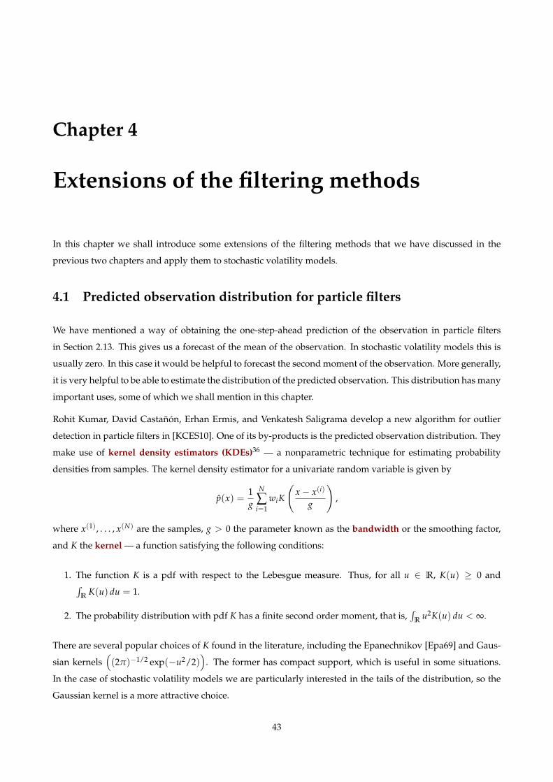
Chapter 4
Extensions of the filtering methods
In this chapter we shall introduce some extensions of the filtering methods that we have discussed in the
previous two chapters and apply them to stochastic volatility models.
4.1 Predicted observation distribution for particle filters
We have mentioned a way of obtaining the one-step-ahead prediction of the observation in particle filters
in Section 2.13. This gives us a forecast of the mean of the observation. In stochastic volatility models this is
usually zero. In this case it would be helpful to forecast the second moment of the observation. More generally,
it is very helpful to be able to estimate the distribution of the predicted observation. This distribution has many
important uses, some of which we shall mention in this chapter.
Rohit Kumar, David Castañón, Erhan Ermis, and Venkatesh Saligrama develop a new algorithm for outlier
detection in particle filters in [KCES10]. One of its by-products is the predicted observation distribution. They
make use of kernel density estimators (KDEs)36 — a nonparametric technique for estimating probability
densities from samples. The kernel density estimator for a univariate random variable is given by
p(x) =1g
N
∑i=1
wiK
(x− x(i)
g
),
where x(1), . . . , x(N) are the samples, g > 0 the parameter known as the bandwidth or the smoothing factor,
and K the kernel — a function satisfying the following conditions:
1. The function K is a pdf with respect to the Lebesgue measure. Thus, for all u ∈ R, K(u) ≥ 0 and∫R
K(u) du = 1.
2. The probability distribution with pdf K has a finite second order moment, that is,∫
Ru2K(u) du < ∞.
There are several popular choices of K found in the literature, including the Epanechnikov [Epa69] and Gaus-
sian kernels((2π)−1/2 exp(−u2/2)
). The former has compact support, which is useful in some situations.
In the case of stochastic volatility models we are particularly interested in the tails of the distribution, so the
Gaussian kernel is a more attractive choice.
43

4.2. Jumps or outliers? 44
While the first moment of the estimated density can be shown to be the sample mean,
∫R
xp(x) =N
∑i=1
wix(i),
the second moment is given by ∫R
x2 p(x) =N
∑i=1
wi
(x(i))2
+ g2κ2,
where κ2 is the second moment of the kernel (1 in the case of the Gaussian kernel), so the variance of the
density p is the sample variance inflated by the factor g2κ2.
This demonstrates by example a general fact — the importance of optimally choosing the bandwidth in kernel
density estimation methods. It is usually chosen to minimise the mean integrated square error (MISE) of the
estimator or other appropriate criteria. The Silverman rule of thumb [Sil86] and Scott bandwidth rule [Sco79]
are often used in practice, but may be suboptimal in a particular situation. Variable bandwidth or adaptive
kernel density estimates may further improve the results. See [Sco15] for details.
We estimate the predicted observation distribution by applying KDE to the samples in (2.12).
4.2 Jumps or outliers?
Gating remains the most common technique for outlier detection in particle filtering. It involves computing
the posterior mean and covariance of the state from t− 1, using the EKF equations (Algorithm 2.5) to compute
a Gaussian approximation to the observation density, then applying the thresholding techniques of Section 2.9.
The posterior density may significantly deviate from Gaussian, as it does in SVLJ. In BayesTSA we imple-
ment the outlier detection method proposed in [KCES10], which involves integrating the KDE of the predicted
observation distribution. Kumar et al. propose an optimisation for the case of zero-mean additive Gaussian
noise. This isn’t the case for SVLJ, so we use Monte Carlo techniques, while noting that in practice this can be
implemented very efficiently [LLP07].
In Figure 4.1 we show the effect of applying different outlier detection thresholds (γ in [KCES10]) in a particle
filter deliberately misspecified to assume that there are no jumps. The RMSE us eventually reduced to a level
approximating that of the correctly specified filter.
4.3 Detecting structural change
The predicted observation distribution can be used to compute the Cumulative Sum of Recursive Resid-
ual (CUSUM) in the same way as it is computed for the Kálmán filter. A description of this statistic and
a case study of its use can be found in [Har89]. For details, see [SG06]. We have included its implementa-
tion in BayesTSA and a plot can be seen in Figure 2.1. It is useful to inspect such plots even in the absence
of automation around change detection. For example, inordinate growth in CUSUM may point out model
misspecification over a particular time interval.

4.4. Resampling 45
Figure 4.1: Comparison of the RMSE for different outlier detection thresholds (γ in [KCES10]) after runningthe filter with smooth resampling schemes. We are averaging the RMSE over 20 runs of the filter on SVLJ datagenerated using StateSpaceModelDataGenerator of the BayesTSA library. We use the same parameters togenerate the data as those in Figure 1 in [PMD14], namely µ = 0.25, φ = 0.975, σ2
v = 0.025, ρ = −0.8, p = 0.01,σ2
J = 10. When running the filter, however, we use the same parameters apart from p, which we assume to bezero (no jumps). The outlier detection mechanism helps reduce the effect of the jumps on the RMSE. Runningthe filter on the correctly specified model (with correct p and σ2
J ) produces RMSE of 0.352 with s.d. 0.035
4.4 Resampling
When particle filters are employed with standard resampling methods, such as the multinomial resampling,
Algorithm 2.2, the resulting simulated likelihood function is not continuous as a function of the parameters
due to the sampling from the discontinuous empirical distribution function (2.2). The smooth resampling
method suggested in [PMD14] to remedy this problem belongs to the category of sampling methods based
on linear interpolation of the empirical distribution function [BCN99, LK00]. This is referred to in [HLD04,
Section 12.1.3] as empirical Law–Kelton (ELK). One weakness of this algorithm is that it generates random
points only between the minimum and maximum of the sample. This limitation is particularly significant in
stochastic volatility models with heavy tails. Several approaches have been suggested to remedy this, such as
the one that named empirical Bratley–Fox–Schrage (EBFS) after [BFS83] in [HLD04]. This method involves
adding an exponential tail to the empirical distribution. It may be appropriate in some situations but is fairly
arbitrary in the context of particle filtering, where any change to the resampling scheme may have serious
implications on the properties of the filter.
On the contrary, the approach based on kernel density estimation [ST95, Section 3.5], [HLD04, Section 12.1.2],
sometimes referred to as smoothed bootstrap has been studied in the particle filter literature. A family of regu-
larised particle filters has been proposed by Christian Musso, Nadia Oudjane, and Françouis Le Gland [MO98,
OM99, MOG01]. In particular, the post-regularised particle filter (post-RPF) [MO98, OM99], which is anal-
ysed theoretically in [GMO98], uses the resampling scheme given as Algorithm 4.1.

4.4. Resampling 46
Figure 4.2: Comparison of the RMSE after running the filter with the smooth [PMD14] and post-RPF (Algo-rithm 4.1) resampling schemes. We are averaging the RMSE over 10–20 runs of the filter on SVLJ data generatedusing StateSpaceModelDataGenerator of the BayesTSA library. Here we have used the same parameters asthose in Figure 1 in [PMD14], namely µ = 0.25, φ = 0.975, σ2
v = 0.025, ρ = −0.8, p = 0.01, σ2J = 10. We assume
that the parameters are known exactly, i.e. we use the same parameters in the particle filter as the ones that weused to generate the data. The error bars show one standard deviation around the mean
Algorithm 4.1 Resampling in the post-regularised particle filter (post-RPF)
Notice that we are working with the normalised weights computed before resampling, brλ(1)t , brλ
(2)t , . . . , brλ
(M)t .
1. Find the appropriate bandwidth g for the kernel density estimator of the empirical distribution given bythe particles x(1)t | t−1, . . . , x(M)
t | t−1 and normalised weights brλ(1)t , . . . , brλ
(M)t (see Section 4.1).
2. Generate M samples from the kernel K, ξ(1), . . . , ξ(M). (This is conveniently done offline.)
3. For i = 1, 2, . . . , M, compute the cumulative sums brΛ(i)t = ∑i
k=1brλ
(k)t , so that, by construction, Λ(M)
t =1.
4. Generate M random samples from U (0, 1), u1, u2, . . . , uM.
5. For each i = 1, . . . , M, choose the particle x(i)t | t := x(j)t | t−1 + gξ(i) with j ∈ 1, 2, . . . , M− 1 such that
ui ∈[
brΛ(j)t , brΛ(j+1)
t
].
Set the normalised weights after resampling: λ(i)t := 1
M .We could view this algorithm as the sampling of posterior particles from the smooth KDE.
Such methods have the theoretical advantage of producing strong approximations of the optimal filter, in
L1 or L2 sense [MOG01, CM14] and, when carefully implemented, introduce little computational over-
head [MOG01]. There is a natural generalisation, using multivariate KDE, to multivariate stochastic volatility
models, such as the ones discussed in [HRS94]. More advanced regularised particle filters can also be em-
ployed, such as L2RPF [MOG01] based on the kernel filter [HK98].

4.5. A generalisation of the Gaussian filter 47
4.5 A generalisation of the Gaussian filter
We have explained in Sections 3.2 and 3.3 why we believe that it is the SVL2 model that is the most consistent
with the Gaussian filter, where the prior estimate of the state at t (given the observations up to and including
the time t − 1) is used to predict the observation at time t. However, we shall derive the filtering equations
for both SVL2 and SVL, since SVL is studied widely in the literature. The Gaussian filter Algorithm 2.7) is not
immediately applicable to these models: we are dealing with correlated non-additive process and observation
noises. The Gaussian approximation recursive filter (GASF) of [WLPY12], where the process and observation
noises are correlated but additive, is not immediately applicable to our problem either. We therefore generalise
Algorithm 2.7 to our problem, beginning with a generalisation of the corresponding Gaussian approximation
Algorithm 2.6:
Algorithm 4.2 Generalised Gaussian moment matching approximation
Let us obtain the moment matching based Gaussian approximation to the joint distribution of the RdX -valued random variable X and the transformed RdY -valued random variable Y , with X = gX(X−, Z) andY = gY(X, Z), where X− ∼ N
(m−, P−
)and Z is an RdZ -valued random variable whose distribution is given
by the pdf pZ. By way of uncurrying, write gY(
gX(X−, Z), Z)
as a function of X− and Z:
g−Y :(X−, Z
)7→ g−Y (X−, Z).
Then (XY
)approx.∼ N
((mµ
),(
P ΞΞᵀ S
)),
where
m =∫
gX(x−, z)ϕ(
x−; m−, P−)
pZ(z) dx− dz,
P =∫ (
gX(x−, z)−m) (
gX(x−, z)−m)ᵀ
ϕ(x−; m−, P−
)pZ(z) dx− dz,
µ =∫
g−Y (x−, z)ϕ(
x−; m−, P−)
pZ(z) dx− dz,
S =∫(g−Y (x−, z)− µ)(g−Y (x−, z)− µ)ᵀϕ
(x−; m−, P−
)pZ(z) dx− dz,
Ξ =∫ (
gX(x−, z)−m) (
gY(x−, z)− µ)ᵀ
ϕ(x−; m−, P−
)pZ(z) dx− dz.
Using the Gaussian moment matching approximation of Algorithm 4.2, we generalise the Gaussian filter to
obtain Algorithm 4.3.

4.6. An application of the Gaussian filter to SVL2 48
Algorithm 4.3 Generalised Gaussian filterThe prediction and update steps of the possibly non-additive noise Gaussian assumed density (Kálmán) filterare:
1. Prediction step:
(a) Predicted (prior) state estimate: xt | t−1 =∫
f t(xt−1, zt)
ϕ(
xt−1; xt−1 | t−1, Pt−1 | t−1
)pZt (zt) dxt−1 dzt.
(b) Predicted (prior) error covariance: Pt | t−1 =∫( f t(xt−1, zt)− xt | t−1)( f t(xt−1, zt)− xt | t−1)
ᵀ
ϕ(
xt−1; xt−1 | t−1, Pt−1 | t−1
)pZt (zt) dxt−1 dzt.
2. Update (or correction) step:
(a) Predicted observation: yt =∫
h−t (xt−1, zt)ϕ(
xt−1; xt−1 | t−1, Pt−1 | t−1
)pZt (zt) dxt−1 dzt.
(b) Innovation (or observation residual): yt = yt − yt.
(c) Innovation covariance: St =∫(h−t (xt−1, zt)− yt)(h
−t (xt−1, zt)− yt)
ᵀ
ϕ(
xt−1; xt−1 | t−1, Pt−1 | t−1
)pZt (zt) dxt−1 dzt.
(d) Crosscovariance: Ξt =∫ (
f t(xt−1, zt)− xt | t−1
) (h−t (xt−1, zt)− yt
)ᵀϕ(
xt−1; xt−1 | t−1, Pt−1 | t−1
)pZt (zt) dxt−1 dzt.
(e) (Optimal) Kálmán gain: Kt = ΞtS−1t .
(f) Updated (posterior) state estimate: xt | t = xt | t−1 + Ktyt.
(g) Updated (posterior) error covariance: Pt | t = Pt | t−1 − KtΞtKᵀt .
4.6 An application of the Gaussian filter to SVL2
Let us now apply Algorithm 4.3, our generalised Gaussian filter, to SVL2. The state equation is consistent with
the standard Kálmán filter paradigm (see Section 2.5). The predict step is, therefore, as in the linear-Gaussian
case:
xt | t−1 = µ(1− φ) + φxt−1 | t−1,
Pt | t−1 = φ2Pt−1 | t−1 + σ2v .
Consider the observation model. Notice that
Proposition 4.6.1. In SVL2, the observation at time t, Yt = (εt − ρσv/2)eXt/2, is a random variable with the gener-
alised NLN distribution of Section 3.3.1,
Yt ∼ NLN
µ′ = −12
ρσv, ν′ = xt | t−1, (σ′χ)2 = 1, (σ′)2 = Pt | t−1, ρ′ =
ρσv√Pt | t−1
,
where we have taken care of the propagation of uncertainty.
Proof. See Appendix A.

4.7. Conclusions, further work, and further reading 49
Substituting the above parameters of the generalised distribution into the equations for E [U], Var [U], and
E [ϑU] in Proposition 3.3.1, we obtain, respectively,
yt = 0, St = ext | t−1+12 Pt | t−1
[1 +
14
ρ2σ2v
], Ξt = e
12 xt | t−1+
18 Pt | t−1 ρσv.
Hence
Kt = e−12 xt | t−1− 3
8 Pt | t−1ρσv
1 + 14 ρ2σ2
v, K2
t Ξt = e−12 xt | t−1− 5
8 Pt | t−1ρ3σ3
v(1 + 1
4 ρ2σ2v
)2 ,
and we obtain the following approximate Gaussian filter for SVL2.
Algorithm 4.4 Generalised Gaussian filter for SVL2The prediction and update steps of the Gaussian filter for SVL2 are:
1. Prediction step:
(a) Predicted (prior) state estimate: xt | t−1 = µ(1− φ) + φxt−1 | t−1.
(b) Predicted (prior) error covariance: Pt | t−1 = φ2Pt−1 | t−1 + σ2v .
2. Update (or correction) step:
(a) Updated (posterior) state estimate: xt | t = xt | t−1 + e−12 xt | t−1− 3
8 Pt | t−1 ρσv
1+ 14 ρ2σ2
vyt.
(b) Updated (posterior) error covariance: Pt | t = Pt | t−1 − e−12 xt | t−1− 5
8 Pt | t−1 ρ3σ3v
(1+ 14 ρ2σ2
v )2 .
For completeness, we give a similar derivation for the SVL2 model without the Stratonovich correction — the
Jacquier–Polson–Rossi model [JPR04] in Appendix B. There the predicted observation will not be zero since in
that model the log-returns don’t form a martingale difference sequence.
4.7 Conclusions, further work, and further reading
We shall now compare the results of running several stochastic filters on generated SVL data. Here we have
used the same parameters as those in Figure 1 in [PMD14], namely µ = 0.25, φ = 0.975, σ2v = 0.025, ρ =
−0.8 with the exception of introducing no jumps, p = 0.01. The outlier detection technique of Section 2.9
could be used in combination with the Kálmán-style filters to deal with jumps, as evidenced by the results
of Section 4.2. The data was generated using the first correlation structure (CS1, as in SVL). We implement a
modification [CLP09] of the unscented Kálmán filter (UKF) [JU96, JU97, WvdM00], which allows correlation
one time step apart, the generalised Gaussian filter for SVL2 (Algorithm 4.4), and a Kálmán filter based on
Harvey’s and Shephard’s QML formulation [HS96]37.
The results are presented in Table 4.1 with graphs and further details in Appendix F. We note that the filters are
not heavily optimised at present and were run on a low-spec machine, so the times should be taken as merely
indicative. While the Harvey–Shephard Kálmán filter is a consistent and asymptotically normal estimator
suitable for quasi-maximum likelihood estimation, it is hardly suitable for real-time filtering due to the large
RMSE.38 The error for the modified UKF is much less, and still less for the generalised Gaussian filter. The
particle filters have a lower RMSE and are, in the limit, optimal. However, the suboptimal filters may be better
suited for the high-frequency trading environment, where the possibility of degeneracy is a major concern and

4.7. Conclusions, further work, and further reading 50
speed is of the essence. The Gaussian filter, which involves only scalar mathematics (unlike both the UKF and
particle filters) can be heavily optimised, especially on specialised low-latency equipment, such as GPUs and
FPGAs.
We repeat the results with lower leverage, ρ = −0.5. The suboptimal filters fare worse in this situation as the
moment-matching approximation deviates further from the true distribution. However, looking at the state
graphs in Appendix F, they continue to track the simulated log-variance at accuracies that may be acceptable
in high-frequency trading applications. In the future one can explore ways of correcting the approximated
distributions for lower values of ρ.
ρ filter RMSE (quasi-) log-likelihood time taken, seconds-0.8 Harvey–Shephard Kálmán filter 1.41 -4889 5.3-0.8 modified UKF 0.67 -3334 6.2-0.8 generalised Gaussian filter 0.52 -3134 4.7-0.8 particle filter for SVL2, post-RPF, 300 particles 0.34 -3080 15.9-0.8 particle filter for SVL, post-RPF, 300 particles 0.30 -3044 17.4-0.5 Harvey–Shephard Kálmán filter 1.41 -4890 5.3-0.5 modified UKF 0.75 -3493 6.7-0.5 generalised Gaussian filter 0.71 -3347 4.7-0.5 particle filter for SVL2, post-RPF, 300 particles 0.39 -3159 16.0-0.5 particle filter for SVL, post-RPF, 300 particles 0.38 -3140 17.9
Table 4.1: A comparison between different stochastic filters applied to generated SVL data

Chapter 5
Intraday stochastic volatility with leverage
5.1 Introduction
The posteriors from the MCMC simulations that we used in Chapter 3 to compare the SVL and SVL2 models
contain some interesting patterns. We see that the leverage effect in the S&P 500 index has been steadily
increasing in recent years (Figure 5.1 (a)). We also note that the leverage effect varies between markets. It
is somewhat less for the European indices (FTSE 100, Euro Stoxx 50, CAC 40, DAX), significantly less for
the Japanese Nikkei 225 and much weaker for the Chinese (SSE Composite) and Russian (MICEX) indices.
While these results do not enable us to draw economic conclusions, it is interesting to plot the macroeconomic
measures of leverage that are available to us — the government debt-to-GDP and households debt-to-GDP
ratios — against the leverage effect (Figure 5.1 (a) and (b)).
Given our interest in medium- to high-frequency trading, we would like to examine what our models tell us
about the leverage effect intraday. Does it continue to exist and what is its relationship to the leverage effect
that we have found in daily log-return data?
5.2 Leverage effect in intraday data
To answer these questions we conduct the following empirical study. We take Dataset 14, containing trades
in S&P 500 E-Mini futures executed on the CME, and Dataset 15, containing trades in Euro Stoxx 50 futures
executed on Eurex. This datasets covers the time interval 2013.04.21–2016.04.21 and contains 274,696,206 and
40,348,422 data points, respectively. That is, on average, 293,165 trades per day for S&P 500 and 43,061 trades
per day for Euro Stoxx 50. The S&P 500 E-Mini futures trade nearly 24/5. For each day we consider the most
actively traded future. We take the last trade before midnight39 to obtain an artificial daily trade price time
series. We compute the log-returns for these prices as detailed in Appendix C to get a time series consisting
of 934 data points. We then take the last trade before midday and the last trade before midnight and obtain
a longer time series of trade prices. We divide this time series into two halves and for each half obtain the
half-daily log-returns. The two resulting time series of log-returns will be roughly equal in length to the
first time-series of daily log-returns. We continue in this manner, further dividing the day into 4, 8, 16, 32,
64, and 128 equal parts obtaining, respectively, 4, 8, 16, 32, 64, and 128 time series of intraday log-returns.
51

5.2. Leverage effect in intraday data 52
(a)
(b) (c)
Figure 5.1: A visual representation of some of the results of Table 3.1 for the SVL model. Subfigure (a) shows theevolution of the leverage, ρ, and volatility of log-variance, σv, parameters for the S&P 500 datasets (Datasets 2–6). Subfigure (b) plots the government debt-to-GDP on the y-axis and leverage for the economy’s key index,ρ, on the x-axis (Japan is an outlier with a very high government debt-to-GDP and has been excluded). Sub-figure (c) plots the households debt-to-GDP on the y-axis and leverage for the economy’s key index, ρ, onthe x-axis. We don’t claim that there is necessarily an economic causal relationship between leverage anddebt-to-GDP and don’t read too much into these plots. Sources: Dataset 7–13, OECD, TradingEconomics.com,TheGlobalEconomy.com — unfortunately we did not have reliable information on corporate or private debt forthe companies underlying each index

5.3. Trade time or wall clock time? 53
Aug 2013 Dec 2013 Apr 2014 Aug 2014 Dec 2014 Apr 2015 Aug 2015 Dec 2015 Apr 2016
time
1.0
0.5
0.0
0.5
1.0
ρτ
Dataset 14, SVL
(a)
5 4 3 2 1 0
ln(τ)
0.9
0.8
0.7
0.6
0.5
0.4
0.3
0.2
0.1
ρτ
Dataset 14, SVL
Dataset 14, SVL2
Dataset 15, SVL
Dataset 15, SVL2
(b)
Figure 5.2: In subfigure (a) we show the leverage effect for each MCMC chain in Dataset 14 under the SVLmodel. The thicker lines correspond to returns computed over longer time periods, the maximum being dailyreturns. Subfigure (b) shows the average leverage for each log-return interval, τ, (measured in units of days)for both datasets under both the SVL and SVL2 models.
We then run the MCMC simulation on each resulting time series of log-returns, 255 Markov chains in total.
The length of each series should be sufficient to maximise the chances of the Markov chain converging. The
univariate posterior distribution of the leverage parameter, ρ, gives us information about the leverage effect
at each frequency of log-returns according to the SVL (SVL2) model. We take the mean of that distribution as
our estimate. We repeat the same procedure under both SVL and SVL2 for Euro Stoxx 50, the trading in which
covers a somewhat smaller portion of the day, but still enough to give us a sufficiently high number of data
points. We summarise the results in Figure 5.2. Further results can be found in Figure E.15 in Appendix E.
We find that ρτ , our estimate of the leverage for log-returns computed over the fraction of the day τ (τ = 1 for
daily log-returns, τ = 1/2 for half-daily, etc.), is related to the leverage for the daily returns by
ρτ ≈ −0.13 ln(τ) + ρ,
where ρ is the estimate of leverage from daily log-returns. Thus both the SVL and SVL2 models suggest that
the leverage effect is present in intraday data and its estimate decreases as the frequency of that data increases.
5.3 Trade time or wall clock time?
We wonder whether leverage is indeed dependent on the time scale or it is obscured by microstructure effects
on intraday timescale. The analysis we applied so far was done in real-world or wall-clock time (taking into
account the real-world time intervals between the trades, which may vary from one trade to another). We
could go beyond the last value interpolation and consider actual wall-clock time intervals between the trades.
We use the Euler–Maruyama discretisation of Section 3.2 to rewrite the SVL model preserving the wall-clock

5.4. Conclusions, further work, and further reading 54
time differences between the ticks:
yt | xt, ρ, τt =√
τtext/2εt,
xt+1 | xt, µ, φ, σ2v , ρ, τt = τt(1− φ)µ + (1− τt(1− φ))xt +
√τtσvηt,
where, as before, (εtηt
)∼ N (0, Σ) , Σ =
(1 ρρ 1
),
and τt is the difference between the wall-clock times at ticks t + 1 and t. We refer to the resulting model as
wall-clock stochastic volatility with leverage (wcSVL). When each τt = 1 we recover the SVL model.
Proposition 5.3.1. The transition density for wcSVL is given by
Xt+1 | xt, µ, φ, σ2v , τt ∼ N
(τt(1− φ)µ + (1− τt(1− φ))xt, τtσ
2v
),
and the likelihood by
Yt | xt+1, xt, µ, φ, σ2v , ρ, τt ∼ N
(√τtext/2 ρ√
τtσvxt+1 − τt(1− φ)µ− (1− τt(1− φ))xt , τtext(1− ρ2)
).
A BUGS implementation of this model is given in Appendix E. To compute the Bayes factors we also need an
adaptation of the particle filtering algorithm:
Algorithm 5.1 An adaptation of the particle filter Algorithm 5.1 to wcSVL
A particle filtering algorithm is obtained by writing, as in the case of SVL, ηt = ρεt +√
1− ρ2ξt, where
ξti.i.d.∼ N (0, 1). In the absence of jumps there is no need to sample ε
(i)t−1. We use the fact that εt = ytτ
−1/2t e−xt/2
to obtain the transition density
Xt+1 | xt, yt, µ, phi, σ2v , ρ, τ ∼ N
(τt(1− φ)µ + (1− τt(1− φ))xt + σvρyte−xt/2, τtσ
2v (1− ρ2)
)and use it to sample the particles x(i)t | t−1. The weights are given by the observation density
p(yt | x(i)t | t−1) = (2πτtex(i)t | t−1)−1/2 exp
(−y2
t /(2τtex(i)t | t−1)
).
We compare the results of calibrating the wcSVL and SVL to the actual intraday trade time-series for the S&P
E-Mini future ESM16 over the time interval 2016.01.01–2016.01.31. This time series of log-returns contains
18,648 points. wcSVL uses the wall-clock time with time measured in days. SVL uses the trade time: each
trade corresponds to a tick, intervals between such ticks regarded as equal. MCMC calibration of wcSVL fails
to find a significant leverage effect, whereas at the tick level we recover a high level of leverage (ρ = −0.91).
5.4 Conclusions, further work, and further reading
These findings seem to agree with those in [ASFL13], where a strong leverage effect is found in high-frequency
data once the sources of bias are taken care of. In order to make our models realistic at higher frequencies, we
need to incorporate the microstructure effects, such as those considered in this paper. Unfortunately, serious
microstructure analysis [Lit04, BLT06, ASFL13] of the stochastic volatility models is beyond the scope of the
present work.

Conclusions and further work
We have applied a combination of stochastic filtering and MCMC techniques to problems in electronic trading,
especially stochastic volatility models with leverage, and examined their performance on simulated data and
actual datasets. We have only considered univariate stochastic volatility models. Extensions to multivariate
models [HRS94] and cointegration [Meu10], perhaps by considering multivariate OU processes, would be
interesting.
Particle filtering methods, while they incur significant computational cost, achieve close-to-optimal RMSE
in nonlinear problems, such as stochastic volatility with jumps. Applying regularisation helps reduce this
RMSE further while keeping the objective function smooth for maximum likelihood parameter estimation.
It may be worthwhile to explore extensions to variable, adaptive bandwidth KDE, e.g. using the approach
suggested in [SS10] to further improve regularised particle filters. In the high-frequency setting, the Gauss
transform [ED03, BY05] could be used to speed up the computation of the cost functions in [SS10]. One could
also explore better ways of sampling directly from the regularised product of the likelihood and the posterior,
e.g. using [MB04]. We have seen how recently introduced methods of outlier detection can help particle filters
in the presence of jumps. Outlier detection can also be used in combination with the Gaussian filter to achieve
the requisite speed in a high-frequency trading setting. To further improve the performance of the filters it
would be interesting to implement them on specialised equipment, such as GPUs and FPGAs.
Our consideration of an alternative discretisation of the stochastic volatility model, and generalisation of Gaus-
sian filter to arbitrary (non-additive) correlated noises, have given rise to a fast approximate filter for stochas-
tic volatility with leverage particularly suited to a high-frequency trading environment, where it is essential
to minimise latency and maximise throughput while processing high-frequency data online. Unlike the un-
scented Kálmán and particle filters, our assumed density filter involves only scalar calculations. In the future,
the moment-matching approximation can be modified to achieve lower RMSE in low leverage settings. We
began to consider the properties of the Gaussian filter and the generalised NLN mixture distribution. More
work is required to understand them properly. Likewise, more thorough work is needed on the filtering Euler–
Maruyama scheme, along the lines of [MSG11].
In our analysis we picked futures with bid-offer spreads small compared with volatility. The observation func-
tion could incorporate the Roll model [Rol84] or its descendants in much the same way as it can incorporate
jumps. MCMC analyses has already been applied to Roll model [Has09, Has10]. It would be useful to incor-
porate stochastic volatility into these models. Further work is needed to account for microstructure effects in
higher-frequency datasets [Lit04, BLT06, ASFL13].
55

Appendix A
Proofs
A.1 Introduction
We have moved some proofs from the main chapters of the dissertation to this appendix to avoid interrupting
the flow of the discussion.
A.2 Proofs for Chapter 3
Lemma A.2.1 (for the proof of Proposition 3.3.1). Let ϑ ∼ N(ν, σ2). For a, b ∈ R, and an integrable function f ,
E[
f (ϑ)eaϑ+b]= eaν+ 1
2 a2σ2+b∫ ∞
−∞f (ϑ)ϕ
(ϑ; ν + aσ2, σ2
)dϑ.
Proof.
E[
f (ϑ)eaϑ+b]= eb
∫ ∞
−∞f (ϑ)eaϑpdfϑ(ϑ) dϑ
= eb∫ ∞
−∞f (ϑ)eaϑ 1√
2πσ2e−(ϑ−ν)2
2σ2 dϑ
= eb∫ ∞
−∞f (ϑ)
1√2πσ2
e−(ϑ−(ν+aσ2))
2+2aνσ2+a2σ4
2σ2 dϑ
= eaν+ 12 a2σ2+b
∫ ∞
−∞f (ϑ)ϕ
(ϑ; ν + aσ2, σ2
)dϑ.
Proposition A.2.2 (Properties of the NLN mixture distribution, i.e. the generalised NLN mixture distribution
with µ = ν = 0 [Yan04], needed for the proof of Proposition 3.3.1). Let U ∼ NLN(σ2, ρ).
1. The conditional distribution of U given ϑ = a is N((ρ/σ)ae
12 a, (1− ρ2)ea
).
2. The mean of U is given by E [U] = 12 ρσe
18 σ2
.
3. The variance of U is given by Var [U] = e12 σ2[1 + ρ2σ2
(1− 1
4 e−14 σ2)]
.
56

A.2. Proofs for Chapter 3 57
Proof of Proposition 3.3.1. 1. Using the substitutions χ′ = (χ− µ)/σχ, ϑ′ = ϑ− ν, we can write U as
U = (µ + σχχ′)e12 (ν+ϑ′) = µe
12 (ϑ′+ν) + σχe
12 νU′,
where U′ = χ′e12 ϑ′ ∼ NLN(σ2, ρ),(
χ′
ϑ′
)∼ N
((00
),(
1 ρσρσ σ2
)).
The result follows by Proposition A.2.2 and the properties of linearly transformed normal random vari-
ables.
2. We can write χ as χ = ρσ (ϑ− ν) + µ + ξ, where ξ is a random variable independent of ϑ and such
that E [ξ] = 0. The variance on the right-hand side must match the variance on the left-hand side,
Var [χ] = σ2χ, Var [ξ] = σ2
χ − ρ2.
E [U] = E[ ρ
σ(ϑ− ν) + µ + ξ
e
12 ϑ]
linearity=
ρ
σE[ϑe
12 ϑ]+(
µ− ρ
σν)
E[e
12 ϑ]+ E[ξe
12 ϑ]
independence=
ρ
σE[ϑe
12 ϑ]+(
µ− ρ
σν)
E[e
12 ϑ]+ E [ξ]E
[e
12 ϑ]
Lemma A.2.1=
ρ
σe
18 σ2+ 1
2 ν∫ ∞
−∞ϑϕ
(ϑ; ν +
12
σ2, σ2)
dϑ +(
µ− ρ
σν)
e18 σ2+ 1
2 ν∫ ∞
−∞ϕ
(ϑ; ν +
12
σ2, σ2)
dϑ,
where the first integral is the first moment of N(
ν + 12 σ2, σ2
), i.e. ν + 1
2 σ2, and the second integral is of
a pdf over its domain, and so equal to 1.
3. We use the same expansion of ξ to find the second moment
E[U2]= E
[ ρ
σ(ϑ− ν) + µ + ξ
2eϑ
]= E
[2(
µ− ρν
σ
)ξeϑ +
2ρ
σξϑeϑ + ξ2eϑ +
(ρ2ν2
σ2 −2ρνµ
σ+ µ2
)eϑ +
2ρ
σ
(µ− ρν
σ
)ϑeϑ +
ρ2
σ2 ϑ2eϑ
]linearity= 2
(µ− ρν
σ
)E[ξeϑ]+
2ρ
σE[ξϑeϑ
]+ E
[ξ2eϑ
]+
(ρ2ν2
σ2 −2ρνµ
σ+ µ2
)E[eϑ]
+2ρ
σ
(µ− ρν
σ
)E[ϑeϑ]+
ρ2
σ2 E[ϑ2eϑ
]independence
= 2(
µ− ρν
σ
)E [ξ]E
[eϑ]+
2ρ
σE [ξ]E
[ϑeϑ]+ E
[ξ2]
E[eϑ]+
(ρ2ν2
σ2 −2ρνµ
σ+ µ2
)E[eϑ]
+2ρ
σ
(µ− ρν
σ
)E[ϑeϑ]+
ρ2
σ2 E[ϑ2eϑ
].
We obtain the result by substituting into the above equation E [ξ] = 0, E[ξ2] = Var
[ξ2] = σ2
χ − ρ2 and,
as a consequence of Lemma A.2.1,
E[eϑ]= eν+ 1
2 σ2,
E[ϑeϑ]= eν+ 1
2 σ2(
ν + σ2)
,
E[ϑ2eϑ
]= eν+ 1
2 σ2(
ν2 + 2νσ2 + σ2 + σ4)
.
4. Follows from Var [U] = E[U2]− (E [U])2 and the two previous items of this proposition.

A.2. Proofs for Chapter 3 58
5. Finally,
E [ϑU] = E[ϑ ρ
σ(ϑ− ν) + µ + ξ
e
12 ϑ]
linearity=
ρ
σE[ϑ2e
12 ϑ]+(
µ− ρν
σ
)E[ϑe
12 ϑ]+ E
[ξϑe
12 ϑ]
independence=
ρ
σE[ϑ2e
12 ϑ]+(
µ− ρν
σ
)E[ϑe
12 ϑ]+ E [ξ]E
[ϑe
12 ϑ]
,
where E [ξ] = 0 and, by Lemma A.2.1,
E[ϑe
12 ϑ]= e
12 ν+ 1
8 σ2(
ν +12
σ2)
,
E[ϑ2e
12 ϑ]= e
12 ν+ 1
8 σ2(
ν2 + νσ2 + σ2 + σ4)
.
Proof of Proposition 3.3.2. By the linearity of the conditional expectation operator,
E [Yt+1 | Yt, Xt] = E[εt+1eXt+1/2 | Yt, Xt
]− 1
2ρσvE
[eXt+1/2 | Yt, Xt
].
We show that the second term, the one being subtracted, is equal to the first. Clearly, Xt+1 | Yt, Xt is normal
and its conditional mean and variance are given by, respectively,
E [Xt+1 | Yt, Xt] = µ(1− φ) + φXt, Var [Xt+1 | Yt, Xt] = σ2v .
Let MZ denote the moment-generating function of a N (m, v) random variable Z (m being its mean and v its
variance), MZ(t) := E[etZ] = emt+vt2/2, t ∈ R. Then
E[eXt+1/2 | Yt, Xt
]= MXt+1 | Yt ,Xt
(1/2) = e12 µ(1−φ)+ 1
2 φXt+18 σ2
v .
By the properties of the NLN mixture distribution,
E[εt+1eXt+1/2 | Yt, Xt
]=
12
ρσve12 µ(1−φ)+ 1
2 φXt+18 σ2
v .
Thus E [Yt+1 | Yt, Xt] = 0 and we see that the log-returns do indeed form a martingale difference sequence.
Proof of Proposition 3.3.3. From the observation and process equations for the SVL2 model, respectively,
yt | xt, ρ = ext/2(
εt −12
ρσv
), (A.1)
xt | xt−1, µ, φ, σ2v , ρ = µ + φ(xt−1 − µ) + ηt, (A.2)
with (εtηt
)i.i.d.∼ N
((00
),(
1 ρρ σ2
v
)),
we obtain the likelihood as follows. If Z1 and Z2 have the bivariate normal distribution with means µ1 and µ2
and variances σ21 and σ2
2 , respectively, and correlation ρ, then the conditional distribution of Z2 given Z1 = z1
is (univariate) normal with
E [Z2 | Z1 = z1] = µ2 + ρσ2(z1 − µ1)
σ1, Var [Z2 | Z1 = z1] = (1− ρ2)σ2
2 .

A.3. Proofs for Chapter 4 59
Since
Xt | xt−1, µ, φ, σ2v ∼ N
(µ + φ(xt−1 − µ), σ2
v
), (A.3)
and (εtXt
)| xt−1, µ, φ, σ2
v , ρ ∼ N((
0µ + φ(xt−1 − µ)
),(
1 ρρ σ2
v
)), (A.4)
Yt | xt, xt−1, µ, φ, σ2v , ρ is normal with
E[Yt | xt, xt−1, µ, φ, σ2
v , ρ]= ext/2E
[εt | xt, xt−1, µ, φ, σ2
v , ρ]− 1
2ext/2ρσv
= ext/2 ρ
σv
(xt − µ− φ(xt−1 − µ)− 1
2σ2
v
),
Var[Yt | xt, xt−1, µ, φ, σ2
v , ρ]= ext Var
[εt −
12
ρσv | xt, xt−1, µ, φ, σ2v , ρ
]= ext(1− ρ2),
the variance being as in SVL.
A.3 Proofs for Chapter 4
Proof of Proposition 4.6.1.
µ′ = E
[εt −
12
ρσv
]= −1
2ρσv;
ν′ = E [Xt]
= E
[µ(1− φ) + φXt−1 + ρσvεt +
√1− ρ2σvξt
]linearity= µ(1− φ) + φE [Xt−1] + ρσvE [εt] =
√1− ρ2σvE [ξt]
= µ(1− φ) + φxt−1 | t−1 + ρσv · 0 +√
1− ρ2σv · 0
= xt | t−1;
(σ′χ)2 = Var
[εt −
12
ρσv
]= 1;
(σ′)2 = Var [Xt]
= Var[
µ(1− φ) + φXt−1 + ρσvεt +√
1− ρ2σvξt
]= Var
[φXt−1 + ρσvεt +
√1− ρ2σvξt
]independence
= Var [φXt−1] + Var [ρσvεt] + Var[√
1− ρ2σvξt
]= φ2Var [Xt−1] + ρ2σ2
v Var [εt] + (1− ρ2)σ2v Var [ξt]
= φ2Pt−1 | t−1 + ρ2σ2v + (1− ρ2)σ2
v
= Pt | t−1;

A.3. Proofs for Chapter 4 60
finally,
ρ′ = Cor [Xt, εt]
=Cov [Xt, εt]√Var [Xt]Var [εt]
=1√
Pt | t−1
·E [(Xt −E [Xt])(εt −E [εt])]
=1√
Pt | t−1
·E[(
µ(1− φ) + φXt−1 + ρσvεt +√
1− ρ2σvξt − µ(1− φ)− φxt−1 | t−1
)εt
]linearity=
1√Pt | t−1
·(
φE [Xt−1εt] + ρσvE[ε2
t
]+√
1− ρ2σvE [ξtεt]− φE[
xt−1 | t−1εt
])independence
=1√
Pt | t−1
·(
φE [Xt−1]E [εt] + ρσvE[ε2
t
]+√
1− ρ2σvE [ξt]E [εt]− φE[
xt−1 | t−1
]E [εt]
)
=ρσv√Pt | t−1
.

Appendix B
Derivation of the Gaussian filter for theJacquier–Polson–Rossi model
We derived a Gaussian filter for SVL2 in Section 4.6. In this appendix we derive it for SVL without the
Stratonovich correction — the Jacquier–Polson–Rossi model [JPR04]. The process model is the same as in
SVL2, so the prediction step of the filter will be the same as in Algorithm 4.4. Let us consider the observation
model.
Proposition B.0.1. In Jacquier–Polson–Rossi, the observation at time t, Yt = εteXt/2, is a random variable with the
generalised NLN distribution of Section 3.3.1,
Yt ∼ NLN
µ′ = 0, ν′ = xt | t−1, (σ′χ)2 = 1, (σ′)2 = Pt | t−1, ρ′ =
ρσv√Pt | t−1
.
Substituting the above parameters of the generalised distribution into the equations for E [U], Var [U], and
E [ϑU] in Proposition 3.3.1, we obtain, respectively,
yt =12
e12 xt | t−1+
18 Pt | t−1 ρσv,
St = ext | t−1+12 Pt | t−1
[1 + ρ2σ2
v
(1− 1
4e−
14 Pt | t−1
)],
Ξt = e12 xt | t−1+
18 Pt | t−1 ρσv
(12
xt | t−1 +14
Pt | t−1 + 1)− xt | t−1yt
= e12 xt | t−1+
18 Pt | t−1 ρσv
(1 +
14
Pt | t−1
).
Hence
Kt = e−12 xt | t−1− 3
8 Pt | t−1ρσv
(1 + 1
4 Pt | t−1
)1 + ρ2σ2
v
(1− 1
4 e−14 Pt | t−1
) ,
K2t Ξt = e−
12 xt | t−1− 5
8 Pt | t−1ρ3σ3
v
(1 + 1
4 Pt | t−1
)3
[1 + ρ2σ2
v
(1− 1
4 e−14 Pt | t−1
)]2 ,
61

62
and we obtain the following approximate Gaussian filter for Jacquier–Polson–Rossi — Algorithm B.1.
Algorithm B.1 Generalised Gaussian filter for the Jacquier–Polson–Rossi modelThe prediction and update steps of the Gaussian filter for the Jacquier–Polson–Rossi model are:
1. Prediction step:
(a) Predicted (prior) state estimate: xt | t−1 = µ(1− φ) + φxt−1 | t−1.
(b) Predicted (prior) error covariance: Pt | t−1 = φ2Pt−1 | t−1 + σ2v .
2. Update (or correction) step:
(a) Predicted observation: yt =12 e
12 xt | t−1+
18 Pt | t−1 ρσv.
(b) Innovation (or observation residual): yt = yt − yt.
(c) Updated (posterior) state estimate: xt | t = xt | t−1 + e−12 xt | t−1− 3
8 Pt | t−1ρσv(1+ 1
4 Pt | t−1)
1+ρ2σ2v
(1− 1
4 e−14 Pt | t−1
) yt.
(d) Updated (posterior) error covariance: Pt | t = Pt | t−1 − e−12 xt | t−1− 5
8 Pt | t−1ρ3σ3
v (1+ 14 Pt | t−1)
3[1+ρ2σ2
v
(1− 1
4 e−14 Pt | t−1
)]2 .

Appendix C
Description of the datasets used inempirical work
C.1 Introduction
In this appendix we shall briefly describe the datasets that we investigate in our empirical work. When our
goal was to compare our results with those obtained by other researchers, we strived, as far as possible, to
reproduce the datasets that they used in their empirical analyses. In other places we considered datasets which
have not been examined elsewhere in the academic literature to the best of our knowledge. This includes the
high-frequency datasets that we have examined.
We refer to all datasets using the notation “Dataset N”, N ∈N∗, throughout the text.
C.2 Financial quantities
Before we describe the datasets per se, we shall briefly consider the financial quantities that we examine in this
work and justify our choices. We are primarily interested in the dynamics of asset prices — i.e., how the asset
prices change over time. Working in discrete time, T := N0, there are several choices for representing price
changes. For t ∈N∗,
Y∗t = St + Dt − St−1,
Y′t = (St + Dt − St−1)/St−1,
Yt = ln(St + Dt)− ln(St−1).
Here St is the price of the asset in units of currency, Dt is the dividend or interest that would be received by
the investor for this particular asset.
There is a good reason for taking differences (differencing) from the point of view of econometrics: the time
series of prices is unlikely to be stationary; taking differences between consecutive observations removes non-
stationarity.
The first differences, Y∗t , are expressed in the same units as St. This makes it difficult to compare the quantity
Y∗t across multiple assets: for example, for some assets, Y∗t will be expressed in cents, for other, in dollars,
63

C.2. Financial quantities 64
etc. For each particular asset, its price units are fairly arbitrary. Both Y′t and Yt are dimensionless40, so don’t
suffer from this drawback. Another disadvantage of Y∗t was mentioned as early as [Fam65]: the variance of
Y∗t , somewhat spuriously, increases with the level of the price, St. Finally, as investors, rather than as purely
theoretical econometricians, we are interested in how much money we make due to price changes (possibly
including the dividends, etc.), in proportion to the value of the assets. This Y∗t cannot provide. Therefore we
shall not use Y∗t in our modelling.
The quantity Y′t is variously referred to as the simple net return, simple return, linear return, proportional
net return, and arithmetic return over the time interval between t− 1 and t. We can “gross it up” to obtain the
simple gross return (also known as proportional gross return and geometric return):
gY′t = (St + Dt)/St−1 = Y′t + 1.
Note that it is customary to call Y′t and gY′t , respectively, the simple net return and simple gross return at time
t. While customary, this is also somewhat sloppy: there are two times, t− 1 and t, in the definitions of these
returns. Because these (discrete) times differ by 1, we call these single-period returns. This caveat will apply
to other kinds of return defined in this section. The time interval [t− 1, t] is called the holding period. The
simple gross return can be interpreted as the future value of one unit of cash invested in the asset for the
holding period [t− 1, t].
The quantity Yt is called the continuously compounded return41 or logarithmic return (log-return for short).
The quantities Y′t , gY′t , and Yt are related to each other via the following equations:
Y′t =gY′t − 1 = exp(Yt)− 1,
gY′t = Y′t + 1 = exp(Yt),
Yt = ln(gY′t ) = ln(Y′t + 1).
By Taylor’s theorem, the expansion of ln(x + 1), where |x| < 1, around the point x = 0 is given by
ln(x + 1) =k
∑n=1
(−1)k+1 xk
k+ o
(|x|k
).
Hence, for |Y′t | < 1,
Yt = ln(Y′t + 1) = Y′t + O(|Y′t |2),
in other words, simple net returns of small absolute value are approximately equal to logarithmic returns.
Since daily returns outside the range from -0.1 to 0.1, i.e. -10% to 10%, are rare, Yt and Y′t are very close.
However, Yt is more convenient mathematically for several reasons. First, it is associated with the logarithmic
price (log-price for short), Mt := ln(St). When Dt = 0,
Yt = Mt −Mt−1.
Chartists42, in particular, prefer to think in terms of log-prices. The vertical distance between two points on
a price time series plot will be in units of price, which, as we said, are fairly arbitrary. Whereas the vertical

C.3. Datasets 65
distance on a log-price time series plot will be (approximately) the percentage difference between the prices:
say P1 = P0 + εP0 for some fraction −1 < ε < 1; then
M1 −M0 = ln(P1)− ln(P0) = ln(P0[1 + ε])− ln(P0) = ln(1 + ε) ≈ ε− 12
ε2 +13
ε3 − . . . ≈ ε.
The logarithmic transform helps stabilise the variance of the time series similarly to how differencing sta-
bilises the mean. As we have mentioned in Section 1.2, log-prices grow linearly in time, whereas prices grow
exponentially.
Another mathematical convenience of the log-returns, Yt, is their additivity across time intervals. We have
already mentioned that there are two times associated with each return. All returns considered so far are
single-period returns. We shall use the notation Yt,K, Y′t,K, etc., to denote K-period returns, so that Yt,1 = Yt,
Y′t,K = Y′t , etc. Ignoring the dividends,
Y∗t,K = St − St−K,
Y′t,K = (St − St−K)/St−K,
gY′t,K = St/St−K,
Yt,K = ln(St)− ln(St−K).
Writing these multi-period returns in terms of single-period returns, we get
Y∗t,K = [St−K+1 − St−K] + [St−K+2 − St−K+1] + . . . + [St − St−1] =K
∑k=1
Y∗t−K+k,
gY′t,K =St−K+1
St−K· St−K+2
St−K+1· . . . · St
St−1=
K
∏k=1
gY′t−K+k,
Y′t,K = St/St−K − 1 =St−K+1
St−K· St−K+2
St−K+1· . . . · St
St−1− 1 =
K
∏k=1
gY′t−K+k − 1,
Yt,K = [Mt−K+1 −Mt−K] + [Mt−K+2 −Mt−K+1] + . . . + [Mt −Mt−1] =K
∑k=1
Yt−K+k.
Thus only Y∗t,K and Yt,K can be expressed as sums of single-period returns. We have already listed many reasons
not to use Y∗t,K. However, this additivity across time intervals gives Yt,K a certain advantage over Y′t,K. We shall
therefore prefer Yt,K in our modelling.43
All definitions of returns mentioned so far ignore inflation and therefore give what an economist would call
nominal results. All of these returns can therefore also be described as nominal. Real returns are obtained
from nominal returns by subtracting adjustments for inflation. Over relatively short time periods these adjust-
ments are difficult to compute. Therefore it is conventional to consider nominal returns in higher-frequency
econometrics, and we shall follow suit.
C.3 Datasets
We shall now describe the datasets that we have used in empirical work. See Table C.1 for a summary.

C.3. Datasets 66
Dataset 1
This dataset is derived from of a time series of daily GBP/USD exchange rates, (St)t=0,1,...,n, n = 945, from
1981.10.01 to 1985.06.28, both inclusive. Logarithmic (continuously compounded) daily returns were com-
puted, scaled by 100, and the resulting time series was mean-adjusted:
Xt = 100 ·[
ln St − ln St−1 −1n
n
∑u=1
(ln Su − ln Su−1)
], t = 1, 2, . . . n. (C.1)
This dataset has been extensively studied in the literature [HRS94, SP97, KSC98, DK00, MY00]. We obtained
it as part of the course materials for [Mey10], which are publicly available for download. It is not clear which
fixing was used as the daily exchange rate to generate the dataset. We attempted to reconstruct the dataset
using a time series of WM/Reuters44 fixes and noticed significant differences. Meyer’s time series was also
longer than that provided by Reuters by eight points. We chose to use Meyer’s dataset without modifications
for the sake of reproducibility.
Dataset 2
This dataset is derived from a time series of daily closing prices of the Standard & Poor’s (S&P) 500, a stock
market index based on the market capitalisations of 500 large companies with common stock listed on the New
York Stock Exchange (NYSE) or NASDAQ. The data was provided by the Yahoo! Finance service. The closing
prices were adjusted for all applicable splits and dividend distributions by Yahoo! in adherence to Center
for Research in Security Prices (CRSP) standards.45 From the prices, (St)t=0,...,n, n = 2022, for the dates from
1980.01.02 to 1987.12.31, both inclusive, we obtained the time series following equation (C.1). This is one of
the time series used in [Yu05]. We generated the time series ourselves as we didn’t have access to the author’s
input data. The number of data points in our time series matches that reported in [Yu05, p. 172]. We were also
able to reproduce some of the results mentioned in that paper very closely using our time series.
Datasets 3–6
These datasets are chronological continuations of Dataset 2 with the daily log-returns on the S&P 500 in-
dex computed according to (C.1) covering the dates 1988.01.05–1995.12.29, 1996.01.03–2003.12.31, 2004.01.05–
2011.12.30, 2012.01.04–2016.12.02, inclusive. We have kept the size of these datasets close to that of Dataset 2.
Dataset 6 is slightly shorter but still longer than Dataset 1 and is length is sufficient to ensure the convergence
of the chains in MCMC simulations, as verified using CODA. The source of these datasets is the Yahoo! Finance
service.
Datasets 7–13
These are datasets of daily log-returns on equity indices for various markets and countries: FTSE 100
(Dataset 7), Euro Stoxx 50 (Dataset 8), CAC 40 (Dataset 9), DAX (Dataset 10), Nikkei 225 (Dataset 11), SSE Com-
posite (Dataset 12), MICEX (Dataset 13). The sources for these are Bloomberg (Datasets 7, 12, 13) and Yahoo!
Finance (all the rest). The log-returns were computed according to (C.1).

C.4. Summary and further reading 67
Datasets 14, 15
These high-frequency datasets were provided by Tick Data, LLC (http://www.tickdata.com). They consist of
trades in S&P 500 E-Mini futures on the CME Group exchange (Dataset 14) and in Euro Stoxx 50 (Dataset 15)
index futures on the Eurex exchange, over the time period 2013.04.21–2016.04.21. There are, on average, 293,165
trades per day for S&P 500 E-Mini futures and 293,165 trades per day for Euro Stoxx 50 futures. The S&P 500
E-Mini futures trade close to 24/5: weekly trading opens on Sunday at 5pm (CST) and closes on Friday at
3:15pm. Trading is almost 24 hours per day with the exception of scheduled maintenance breaks at 3:15pm–
3:30pm and at 4:15pm–5pm. Continuous trading in Euro Stoxx 50 index futures takes place at 07:50am–10pm
CET.
C.4 Summary and further reading
For further details on the financial quantities that we have discussed here see [Tay05, Chapter 2], [Tsa10, Chap-
ter 1], and [Sol12, Section 4.2].
Table C.1 summarises the datasets that we have used in empirical work and provides some further details
about them.
Dataset Product First date Last date Frequency Points Underlying data Log-return s.d.1 GBP/USD spot 1981.10.01 1985.06.28 daily 945 closes 0.712 S&P 500 index 1980.01.01 1987.12.31 daily 2,022 closes 1.133 S&P 500 index 1988.01.05 1995.12.29 daily 2,021 closes 0.784 S&P 500 index 1996.01.03 2003.12.31 daily 2,014 closes 1.255 S&P 500 index 2004.01.05 2011.12.30 daily 2,014 closes 1.396 S&P 500 index 2012.01.04 2016.12.02 daily 1,238 closes 0.817 FTSE 100 index 2012.01.04 2016.12.02 daily 1,226 closes 0.918 Euro Stoxx 50 index 2012.01.03 2016.12.02 daily 1,208 closes 1.299 CAC 40 index 2012.01.03 2016.12.02 daily 1,259 closes 1.23
10 DAX index 2012.01.04 2015.12.02 daily 1,251 closes 1.2111 Nikkei 225 index 2012.01.05 2015.12.02 daily 1,221 closes 1.4912 SSE Composite index 2012.01.05 2015.12.02 daily 1,193 closes 1.5613 MICEX index 2012.01.04 2015.12.02 daily 1,230 closes 1.2214 S&P E-mini index futures 2013.04.21 2016.04.21 intraday 274,696,206 trades15 Euro Stoxx 50 index futures 2013.04.21 2016.04.21 intraday 40,348,422 trades
Table C.1: Summary of the datasets

Appendix D
An overview of frequentist and Bayesianapproaches to estimation
D.1 Introduction
We shall briefly summarise the key distinctions between the frequentist and Bayesian approaches to estima-
tion. The latter originate in the philosophical work of Reverend Thomas Bayes [BP63]. For this discussion to
make sense, we need to first mention the three different interpretations of probability.
D.2 Interpretations of probability
The long-term relative frequency (LTRF) interpretation, also known as frequentist or objectivist, considers
an experiment such that, when it is performed, a certain event A either does or does not occur. Furthermore,
suppose that our experiment is repeatable an arbitrary number of times. Let us denote by N(A, n) the number
of occurrences of A in n repeats of the experiment. Then
P [A] = limn→∞
N(A, n)n
.
In the Bayesian, also known as subjectivist, epistimic or evidential, interpretation of probability we say that
the probability of an event A is the degree of belief that the event A occurs, determined on the basis of empir-
ical observations, past experience or indeed subjective plausibility. This interpretation enables one to assign
probability to an arbitrary statement, irrespective of whether an experiment takes place or is even possible.
The third interpretation of probability is called axiomatic and is due to Andrey Nikolaevich Kolmogorov:
“The theory of probability as a mathematical discipline can and should be developed from axioms in exactly
the same way as Geometry and Algebra” [Kol33]. Thus the difficult philosophical question of what probability
actually is is sidestepped; probability is defined through how it behaves. Kolmogorov’s axioms are consistent
with both the frequentist and Bayesian interpretations of probability; the LTRF interpretation reappers in the
axiomatic interpretation as a theorem — the Strong Law of Large Numbers.
The relative merits of the frequentist and Bayesian interpretations are still subject of much academic discussion.
For example, frequentists point out that the frequentist interpretation of probability is more objective, whereas
68

D.3. Bayes’s theorem 69
the Bayesian interpretation is subjective. Bayesians point out that, in their approach, both new and past data,
as well as belief, are used to draw conclusions, whereas frequentists rely only on past data.
D.3 Bayes’s theorem
Theorem D.3.1 (Bayes’s theorem). [BP63] Let H and E be events. The central theorem of Bayesian thinking, Bayes’s
theorem, establishes the relationship between the probability of H, P [H], the probability of E, P [E], the conditional
probability of H given E, P [H | E], and the conditional probability of E given H, P [E | H]:
P [H | E] =P [E | H]P [H]
P [E].
As we said above, the frequentist thinks of the unconditional probability as the proportion of outcomes of an
experiment, in other words, a frequency, when the event occurs. By the same token, conditional probabilities
are interpreted as relative frequencies: for example, P [H | E] is the proportion of outcomes when the event H
occurs out of those when the event E occurs. Formally,
P [H] := limn→∞
N(H, n)n
, P [E] := limn→∞
N(E, n)n
,
P [H | E] =P [H ∩ E]
P [E]= lim
n→∞
N(H ∩ E, n)N(E, n)
, P [E | H] =P [H ∩ E]
P [H]= lim
n→∞
N(H ∩ E, n)N(H, n)
.
Thus a frequentist interprets Bayes’s theorem as a way or relating the relative frequencies P [H | E] and
P [E | H].
How does a Bayesian interpret Bayes’s theorem? Before answering this question, let us introduce some termi-
nology. For a Bayesian, probability is a degree of belief. Before (prior to) any observation, we are talking about
the degree of belief in a certain hypothesis, H. We call this probability, P [H], the prior, the initial degree of
belief in H. We then consider a particular piece of evidence, E. After (posterior to) taking this piece of evidence
into account, we update our degree of belief, obtaining the posterior probability P [H | E].
The ratio P [E | H] /P [E] is sometimes referred to as the support that E provides for H. The conditional
probability P [E | H] is the likelihood, the compatibility of the evidence with the hypothesis. Finally, P [E] is
the marginal likelihood of the evidence, irrespective of the hypothesis.
Thus, in Bayesian interpretation, Bayes’s theorem says this:
posterior = support · prior ∝ likelihood · prior.
According to an old statistical joke, “a Bayesian is one who, vaguely expecting a horse and catching a glimpse
of a donkey, strongly concludes he has seen a mule” [Sen97].
D.4 Frequentist and Bayesian estimation
Let us now understand how frequentists and Bayesians approach the estimation of unknown parameters in
mathematical models. Let y ∈ Rm be a vector of observed data and let θ ∈ Rn be a vector of parameters.
Given y, we would like to estimate θ.

D.5. Further reading 70
First, let us consider the frequentist approach. Let f (y; θ) be the probability density of y that depends on the
parameters θ. View it as a function of the variable θ with y fixed: L(θ) := f (y; θ). We call L(θ) the likelihood
function. The maximum likelihood estimator (MLE), θML, is the value of θ that maximises the likelihood
function. Notice that we get a single value, θML ∈ Rn, as a result of the optimisation of the likelihood function.
Now let us consider the Bayesian approach. We regard θ as an Rn-valued random variable and y as a (pos-
sibly singleton) set of realisations of an Rm-valued random variable Y . The probability distribution of the
parameters θ expresses our beliefs about their likely values. We start with a prior distribution, π(θ), express-
ing our beliefs about θ before observing y. The likelihood is the conditional density of the data, Y ∈ y,
given θ, f (Y ∈ y | θ). The joint density of Y ∈ y and θ is then the product of the prior and the likeli-
hood: f (Y ∈ y, θ) = π(θ) f (Y ∈ y | θ). The marginal likelihood is the marginal density of Y ∈ y, i.e.
f (Y ∈ y) =∫
π(Y ∈ y | θ) dθ. The conditional density of θ given Y ∈ y, the posterior, is
f (θ | Y ∈ y) =π(θ) f (Y ∈ y | θ)∫π(θ) f (Y ∈ y | θ) dθ
.
For conciseness, it is customary to write y in place of Y ∈ y. The result of a Bayesian estimation procedure is,
then, a probability distribution, rather than a single value as in the case of the frequentist estimation, namely the
posterior f (θ | y).
D.5 Further reading
For a gentle introduction to Bayesian analysis, see [Sto13]. See [Wil01] for more information on interpretations
of probability. Here we consider only the modern notions of probability. Pre-modern notions of probability
were very different and were not numerical [Sch15]. For more details on frequentist and Bayesian approaches
to estimation, see [Rup04, Chapter 2].

Appendix E
Markov chain Monte Carlo analyses inOpenBUGS: implementations,instructions, and results
E.1 Introduction
The instructions given in this appendix apply to OpenBUGS version 3.2.3 rev 1012. Further analyses were
performed using the coda package version 0.18-1 for R (64-bit) version 3.3.2. We ran this software under
Microsoft Windows 10 version 1607 (OS Build 14393.447).
E.2 Implementation of the models in BUGS
We follow the discussions in [MY00, Yu05, Mey10] to reproduce Meyer’s and Yu’s implementations of the basic
SV and SVL models in BUGS:
Listing E.1 An implementation of the SV model in BUGS
model 2 # Priors
mu ∼ dnorm(0., 0.04)4 beta ← exp(.5 * mu)
phistar ∼ dbeta(20., 1.5)6 phi ← 2. * phistar - 1.
recsigmav2 ∼ dgamma(2.5, 0.025)8 sigmav ← sqrt(1. / recsigmav2)
alpha ← (1. - phi) * mu10
# Initial distribution of the state12 x0 ∼ dnorm(mu, recsigmav2)
14 # Transition densityxmean[1] ← alpha + phi * x0
16 x[1] ∼ dnorm(xmean[1], recsigmav2)I(-5,5)for (t in 2:n)
18 xmean[t] ← alpha + phi * x[t-1]x[t] ∼ dnorm(xmean[t], recsigmav2)I(-4,4)
20
22 # Likelihoodfor (t in 1:n)
24 recyvar[t] ← 1. / exp(x[t])
71

E.2. Implementation of the models in BUGS 72
y[t] ∼ dnorm(0, recyvar[t])26
28
# Initial values30 list(mu=0, phistar=0.98, recsigmav2=40)
Listing E.2 An implementation of the SVL model in BUGS
model 2 # Priors
mu ∼ dnorm(0., 0.04)4 beta ← exp(.5 * mu)
phistar ∼ dbeta(20., 1.5)6 phi ← 2. * phistar - 1.
recsigmav2 ∼ dgamma(2.5, 0.025)8 sigmav ← sqrt(1. / recsigmav2)
rho ∼ dunif(-1., 1.)10 alpha ← (1. - phi) * mu
12 # Initial distribution of the statex0 ∼ dnorm(mu, recsigmav2)
14 xmean[1] ← alpha + phi * x0x[1] ∼ dnorm(xmean[1], recsigmav2)I(-5,5)
16
# Transition density18 for (t in 1:n)
xmean[t+1] ← alpha + phi * x[t]20 x[t+1] ∼ dnorm(xmean[t+1], recsigmav2)I(-4,4)
22
# Likelihood24 for (t in 1:n)
ymean[t] ← rho/sigmav * exp(0.5 * x[t]) * (x[t+1] - alpha - phi * x[t])26 recyvar[t] ← 1. / ( exp(x[t]) * (1 - rho*rho) )
y[t] ∼ dnorm(ymean[t], recyvar[t])28
30
# Initial values32 list(mu=0, phistar=0.98, recsigmav2=40, rho=-0.4)
Following Proposition 3.3.3, an implementation of the SVL2 model with the same priors and initial values is
given below.
Listing E.3 An implementation of the SVL2 model in BUGS
model 2 # Priors
mu ∼ dnorm(0., 0.04)4 beta ← exp(.5 * mu)
phistar ∼ dbeta(20, 1.5)6 phi ← 2*phistar - 1
recsigmav2 ∼ dgamma(2.5, 0.025)8 sigmav ← sqrt(1/recsigmav2)
rho ∼ dunif(-1, 1)10 alpha ← mu*(1-phi)
12 # Initial distribution of the statex0 ∼ dnorm(mu, recsigmav2)
14 xmean[1] ← alpha + phi * x0x[1] ∼ dnorm(xmean[1], recsigmav2)I(-5,5)
16
# Transition density18 for (t in 2:n)
xmean[t] ← alpha + phi * x[t-1]20 x[t] ∼ dnorm(xmean[t], recsigmav2)I(-4,4)

E.2. Implementation of the models in BUGS 73
22
# Likelihood24 ymean[1] ← rho/sigmav * exp(0.5 * x[1]) * (x[1] - alpha - phi * x0 - 0.5*sigmav*sigmav)
recyvar[1] ← 1. / ( exp(x[1]) * (1 - rho*rho) )26 y[1] ∼ dnorm(ymean[1], recyvar[1])
for (t in 2:n) 28 ymean[t] ← rho/sigmav * exp(0.5 * x[t]) * (x[t] - alpha - phi*x[t-1] - 0.5*sigmav*sigmav)
recyvar[t] ← 1. / ( exp(x[t]) * (1 - rho*rho) )30 y[t] ∼ dnorm(ymean[t], recyvar[t])
32
34 # Initial valueslist(mu=0, phistar=0.98, recsigmav2=40, rho=-0.4)
Finally, the wcSVL model of Chapter 5 is implemented as follows:
Listing E.4 An implementation of the wcSVL model in BUGS
1 model # Priors
3 mu ∼ dnorm(0., 0.04)beta ← exp(.5 * mu)
5 phistar ∼ dbeta(20., 1.5)phi ← 2. * phistar - 1.
7 recsigmav2 ∼ dgamma(2.5, 0.025)sigmav ← sqrt(1. / recsigmav2)
9 rho ∼ dunif(-1., 1.)oneminusphi ← 1. - phi
11 alpha ← oneminusphi * mu
13 # Initial distribution of the statex0 ∼ dnorm(mu, recsigmav2)
15
# We assume that dt[0] == dt[1] as a corner case17 xmean[1] ← dt[1] * alpha + (1. - dt[1] * oneminusphi) * x0
recxvar[1] ← recsigmav2 / dt[1]19 x[1] ∼ dnorm(xmean[1], recxvar[1])I(-5,5)
21 # Transition densityfor (t in 1:n)
23 xmean[t+1] ← dt[t] * alpha + (1. - dt[t] * oneminusphi) * x[t]recxvar[t+1] ← recsigmav2 / dt[t]
25 x[t+1] ∼ dnorm(xmean[t+1], recxvar[t+1])I(-4,4)
27
# Likelihood29 for (t in 1:n)
ymean[t] ← sqrt(dt[t]) * exp(0.5 * x[t]) * rho / (sqrt(dt[t]) * sigmav) * (x[t+1] - dt[t] *→ alpha - (1. - dt[t] * oneminusphi) * x[t])
31 recyvar[t] ← 1. / ( dt[t] * exp(x[t]) * (1. - rho*rho) )y[t] ∼ dnorm(ymean[t], recyvar[t])
33
35
# Initial values37 list(mu=0, phistar=0.98, recsigmav2=40, rho=-0.4)
Yu uses a normal prior on µ,N (0, 25). Such a prior is called diffuse or uninformative (or, more accurately, not
very informative) as it expresses vague or general information about a parameter. The parameters of a prior,
in this case the mean 0 and variance 25, are called hyperparameters to distinguish them from the parameters
of the model. Notice that BUGS uses precision instead of variance as a parameter of the normal distribution;
precision is the reciprocal (one over) variance:
mu ∼ dnorm(0, 0.04)

E.3. Instructions for running Markov chain Monte Carlo analyses in OpenBUGS 74
Yu uses the same priors as Kim et al. in [KSC98] for φ and σ2v . They write φ as φ = 2φ∗ − 1, where φ∗ ∼
Beta(α = 20, β = 1.5). Thus φ has support (−1, 1) and probability density function
pφ(x) =12· pφ∗
(x + 1
2
),
where pφ∗ is the probability density function of Beta(20, 1.5). The mean of φ is 0.8604 and its variance 0.01153.
σ2v is assumed to follow the inverse-gamma distribution with the shape parameter α = 2.5 and rate parameter
β = 0.025, σ2v ∼ InverseGamma(α = 2.5, β = 0.25), meaning that 1
σ2v∼ Gamma(α = 2.5, β = 0.25). Note that
there are two common parameterisations of the Gamma distribution, Gamma(k, θ), where k > 0 is the shape
parameter, θ > 0 is the scale parameter, and Gamma(α, β), where α > 0 is the shape parameter, β > 0 is the
rate parameter. The corresponding probability density functions being
x 7→ 1Γ(k)θk xk−1e−
xθ , x 7→ βα
Γ(α)xα−1e−βx.
It is the latter that is implemented in BUGS. The mean and variance of this prior are, respectively, 0.1667 and
0.0556. Finally, Yu uses a uniform distribution — a “flat”, uninformative prior — for ρ with support [−1, 1],
and the following initial values for the parameters:
µ = 0, φ = 0.96, σ2v = 0.025, ρ = −0.4.
E.3 Instructions for running Markov chain Monte Carlo analyses inOpenBUGS
Under the directory code, the following directories contain files relevant to BUGS:
• ./datasets: this directory contains the datasets. Each dataset consists of two files, with names having
the following format:
dataset-<i>_y.txtdataset-<i>_n.txt
<i> is the number of the dataset. The datasets are listed in Appendix C, and <i> is consistent with
the numbering convention given there. The first file contains the time series of observations, while the
second initialises n to the number of data points in the dataset. Thus the second file consists a single line.
• ./mcmc: this directory contains the BUGS specifications of the various models examined in the disserta-
tion. The specifications appear under this directory in text files with names <modelname>.txt.
• ./results/mcmc/<modelname>/dataset-<i>: These directories contain the outputs obtained from Open-
BUGS and coda for each combination of (model, dataset).
The instructions below explain how the aforementioned outputs were obtained. First, a combination of
(model, dataset) is selected. In other words, one selects <modelname> and <i>— let’s refer to these choices
as <MODELNAME> and <I>. Then the steps are as follows:

E.3. Instructions for running Markov chain Monte Carlo analyses in OpenBUGS 75
1. Start OpenBUGS.
2. From the menu, select File → Open. In the “Open” dialogue box set the file extension filter to “Text
(*.txt)” (otherwise OpenBUGS will attempt to interpret the file as a OpenBUGS document, *.odc, and the
operation will fail). Browse to mcmc/<modelname>.txt and open it. An editor window will be created.
3. Repeat the above step for datasets/dataset-<i>_y.txt and datasets/dataset-<i>_n.txt. Thus we
end up with two more editor windows.
4. From the menu, select Model→ Specification... The “Specification Tool” dialogue box will appear.
5. In the editor window with <modelname>.txt, highlight the first keyword — model— by double-clicking
on it. Then click on the “check model” button in the “Specification Tool” dialogue box. The status bar at
the bottom of the main OpenBUGS window should show “model is syntactically correct”.
6. In the editor window with the dataset-<i>_n.txt file, highlight the keyword list. In the “Specification
Tool” dialogue, click on “load data”. The status bar should show “data loaded”.
7. In the editor window with the dataset-<i>_y.txt file, highlight the variable name y. In the Specification
Tool dialogue, click on “load data”. The status bar should show “data loaded”.
8. In the Specification Tool dialogue, click on “compile”. The status bar should show “model compiled”.
9. In the editor window with <modelname>.txt, highlight the first keyword in the last line — list. In the
“Specification Tool” dialogue, click on “load inits”. The status bar should show “initial values loaded
but chain contains uninitialized variables”.
10. In Specification Tool dialogue, click on “gen inits”. We have already loaded the initial values for the
parameters such as mu; now we are generating x0. The status bar should show “initial values generated,
model initialized”.
11. Close the Specification Tool dialogue.
12. From the menu, select Model→ Update. In the “Update Tool” dialogue, enter 10000 (ten thousand) in
the “updates” field and 20 in the “refresh” field. Click on “update”. The status bar should show “model
is updating”. You will see the iteration count increasing in the “iteration” field. Wait until this value
reaches 10000. This step may take several minutes depending on the performance of the machine on
which OpenBUGS is being run.
13. We have completed the burn-in. Close the “Update Tool” dialogue.
14. From the menu, select Inference→ Samples... In the “Sample Monitor Tool” dialogue, enter “mu” (omit-
ting the quotation marks) in the “node” field and click on “set”. Repeat for each of “beta”, “phi”,
“sigmav”, “rho” (if this particular parameter is present in model <MODELNAME>). This will create monitors
for these nodes for all update iterations that follow and they will be included in the statistics. We didn’t
add these monitors earlier to ensure that we exclude the burn-in iterations from these statistics.

E.3. Instructions for running Markov chain Monte Carlo analyses in OpenBUGS 76
15. Close the Sample Monitor Tool dialogue.
16. From the menu, select Model → Update. In the “Update Tool” dialogue, enter 100000 (one hundred
thousand) in the “updates” field and 20 in the “refresh” field. Click on “update”. The status bar should
show “model is updating”. You will see the iteration count increasing in the “iteration” field. Wait until
this value reaches 110000 (as this number includes the already completed burn-in iterations). This step
may take 10–30 minutes or more, depending on the model specification and on the performance of the
machine on which OpenBUGS is being run.
17. Close the Update Tool dialogue.
18. From the menu, select Inference→ Samples... In the “Sample Monitor Tool” dialogue, enter “*” in the
“node” field and click on “stats”. You should see the “Node statistics” window with summary statis-
tics. From the menu, select File→ Save As..., set “Save as type” to “Document (*.odc)”, “File name” to
node-statistics.odc and click “Save”. From the menu, select File→ Save As..., set “Save as type” to
“Plain Text (*.txt)”, “File name” to node-statistics.txt and click “Save”.
19. In the “Sample Monitor Tool” dialogue, click on “history”. You should see the “History” window with
plots. From the menu, select File→ Save As..., set “Save as type” to “Document (*.odc)”, “File name” to
history.odc and click “Save”. From the menu, select File → Print..., choose “Microsoft Print to PDF”
under “Select Printer” and click “Print”; set “File name” to history.pdf and click “Save”.
20. In the “Sample Monitor Tool” dialogue, click on “density”. You should see the “Posterior density” win-
dow with kernel-smoothed posterior density plots. From the menu, select File→ Save As..., set “Save as
type” to “Document (*.odc)”, “File name” to posterior-density.odc and click “Save”. From the menu,
select File→ Print..., choose “Microsoft Print to PDF” under “Select Printer” and click “Print”; set “File
name” to posterior-density.pdf and click “Save”.
21. In the “Sample Monitor Tool” dialogue, click on “quantiles”. You should see the “Running quantile”
window with the running quantiles plots. By default, we are showing the percentiles 2.5 and 97.5, and the
median. From the menu, select File→ Save As..., set “Save as type” to “Document (*.odc)”, “File name”
to running-quantiles.odc and click “Save”. From the menu, select File → Print..., choose “Microsoft
Print to PDF” under “Select Printer” and click “Print”; set “File name” to running-quantiles.pdf and
click “Save”.
22. In the “Sample Monitor Tool” dialogue, click on “coda”. You should see the “CODA index” and “CO-
DAchain1” windows — the two inputs for the R package coda. Select the first of these windows.
From the menu, select File → Save As..., set “Save as type” to “Plain Text (*.txt)”, “File name” to
coda-index.txt and click “Save”. Now select the second window. From the menu, select File→ Save
As..., set “Save as type” to “Plain Text (*.txt)”, “File name” to coda-chain-1.txt and click “Save”.
23. In the “Sample Monitor Tool” dialogue, click on “auto cor”. You should see the “Auto-correlation”
window with autocorrelograms. From the menu, select File → Save As..., set “Save as type” to “Doc-
ument (*.odc)”, “File name” to autocorrelation.odc and click “Save”. From the menu, select File →

E.4. Output analysis and diagnostics with coda 77
Print..., choose “Microsoft Print to PDF” under “Select Printer” and click “Print”; set “File name” to
autocorrelation.pdf and click “Save”.
Among the files that we have saved there are three text files, node-statistics.txt, coda-index.txt, and
coda-chain-1.txt. The first of these files presents a useful summary of the node statistics, a bird’s eye
view of the results. The other two will be used by the R package coda. We will talk about these files in
Section E.4. We have saved all graphs as *.pdf documents, so they can easily be included in LATEX reports with
\includegraphics. Finally, we have saved all objects (text and graph) as OpenBUGS documents, *.odc, so we
can open them with OpenBUGS at a later stage.
E.4 Output analysis and diagnostics with coda
coda is an R package that provides functions for summarising and plotting the output from MCMC simula-
tions, as well as diagnostic tests of convergence to the equilibrium distribution of the Markov chain.
To install this package under R, run
install.packages("coda")
Load the coda library:
library(coda)
To analyse the results of a MCMC simulation for a particular (model, dataset), set the R working directory
to the corresponding <modelname>/results-for-dataset-<i> directory:
setwd(".../results/mcmc/<modelname >/dataset-<i>")
Then read the two files with raw data that we saved for coda:
res <- read.coda(’coda-chain -1.txt’, ’coda-index.txt’)
We should see
Abstracting beta ... 100000 valid valuesAbstracting mu ... 100000 valid valuesAbstracting phi ... 100000 valid valuesAbstracting rho ... 100000 valid valuesAbstracting sigmav ... 100000 valid values
Summarise the results of the MCMC simulation:
summary(res)
We save the output as coda-summary.txt. Next, plot the traces and posterior densities46:
plot(res)
We save the two pages of the plot as coda-plots-1.pdf and coda-plots-2.pdf. Finally,
codamenu()
select option 2 (“Use an mcmc object”). When prompted “Enter name of saved object”, enter “res”. Then
select option 2 (“Diagnostics”) from the menu. We run the Geweke, Raftery and Lewis, Heidelberger and
Welch, Autocorrelations, and Cross-Correlations diagnostics, and save the results as coda-diagnostics.txt.

E.5. Results 78
E.5 Results
E.5.1 Summaries: node statistics
Listing E.5 Node statistics for model SV, Dataset 1
node mean sd MC error 2.5% median 97.5% start samplebeta 0.7121 0.114 0.002775 0.5541 0.6894 0.9992 10001 100000mu -0.7022 0.2983 0.007182 -1.181 -0.7438 -0.001617 10001 100000phi 0.9795 0.01105 3.736E-4 0.9538 0.9811 0.996 10001 100000sigmav 0.1567 0.03169 0.001478 0.1039 0.154 0.2273 10001 100000
Listing E.6 Node statistics for model SVL, Dataset 1
node mean sd MC error 2.5% median 97.5% start samplebeta 0.7214 0.128 0.003455 0.5522 0.6939 1.056 10001 100000mu -0.6809 0.3247 0.008484 -1.188 -0.7309 0.1095 10001 100000phi 0.9809 0.01123 3.776E-4 0.9549 0.9827 0.9971 10001 100000rho -0.04357 0.1468 0.004837 -0.3275 -0.04342 0.2401 10001 100000sigmav 0.1549 0.03069 0.001379 0.1032 0.1521 0.2229 10001 100000
Listing E.7 Node statistics for model SVL2, Dataset 1
node mean sd MC error 2.5% median 97.5% start samplebeta 0.7434 0.1442 0.003956 0.5516 0.7114 1.109 10001 100000mu -0.6265 0.3577 0.009804 -1.19 -0.681 0.2075 10001 100000phi 0.9835 0.01091 3.835E-4 0.9575 0.9855 0.9982 10001 100000rho -0.1452 0.1372 0.004488 -0.4141 -0.1445 0.1227 10001 100000sigmav 0.1535 0.03176 0.001478 0.09684 0.1515 0.2213 10001 100000
Listing E.8 Node statistics for model SV, Dataset 2
node mean sd MC error 2.5% median 97.5% start samplebeta 0.8967 0.06348 8.892E-4 0.781 0.8935 1.032 10001 100000mu -0.223 0.1406 0.001954 -0.4944 -0.2251 0.06263 10001 100000phi 0.9736 0.008418 2.893E-4 0.9549 0.9744 0.9879 10001 100000sigmav 0.1517 0.01933 8.596E-4 0.118 0.1502 0.1935 10001 100000
Listing E.9 Node statistics for model SVL, Dataset 2
node mean sd MC error 2.5% median 97.5% start samplebeta 0.8971 0.05707 7.922E-4 0.7914 0.8946 1.018 10001 100000mu -0.2213 0.1265 0.001744 -0.4678 -0.2227 0.03495 10001 100000phi 0.9696 0.00965 3.573E-4 0.948 0.9706 0.9858 10001 100000rho -0.2828 0.08621 0.002662 -0.4463 -0.285 -0.1081 10001 100000sigmav 0.1633 0.02185 9.789E-4 0.1252 0.1614 0.2116 10001 100000
Listing E.10 Node statistics for model SVL2, Dataset 2
node mean sd MC error 2.5% median 97.5% start samplebeta 0.9039 0.06224 9.247E-4 0.7909 0.9003 1.038 10001 100000mu -0.2067 0.1363 0.002001 -0.4691 -0.2101 0.07364 10001 100000phi 0.9746 0.008456 3.11E-4 0.9555 0.9755 0.9887 10001 100000rho -0.2757 0.08773 0.002836 -0.4411 -0.2778 -0.09903 10001 100000sigmav 0.1488 0.01966 8.955E-4 0.114 0.1476 0.1922 10001 100000

E.5. Results 79
Listing E.11 Node statistics for model SVL, Dataset 3
node mean sd MC error 2.5% median 97.5% start samplebeta 0.6908 0.04179 9.988E-4 0.6268 0.6874 0.7713 10001 100000mu -0.7431 0.1124 0.002549 -0.9343 -0.7496 -0.5192 10001 100000phi 0.935 0.01929 7.988E-4 0.8909 0.9369 0.9671 10001 100000rho -0.3497 0.07389 0.001852 -0.4881 -0.352 -0.1974 10001 100000sigmav 0.2664 0.04154 0.001915 0.1918 0.2632 0.3567 10001 100000
Listing E.12 Node statistics for model SVL2, Dataset 3
node mean sd MC error 2.5% median 97.5% start samplebeta 0.7852 0.2352 0.0114 0.6397 0.7212 1.617 10001 100000mu -0.5395 0.4234 0.02044 -0.8935 -0.6536 0.9607 10001 100000phi 0.966 0.01551 7.243E-4 0.9347 0.966 0.9978 10001 100000rho -0.3446 0.08638 0.002877 -0.5113 -0.3451 -0.1754 10001 100000sigmav 0.1864 0.03511 0.001771 0.1171 0.1862 0.2574 10001 100000
Listing E.13 Node statistics for model SVL, Dataset 4
node mean sd MC error 2.5% median 97.5% start samplebeta 1.058 0.049 9.369E-4 0.9623 1.057 1.157 10001 100000mu 0.1105 0.09278 0.001771 -0.07679 0.1116 0.2908 10001 100000phi 0.9707 0.006377 2.419E-4 0.957 0.9711 0.982 10001 100000rho -0.7859 0.0463 0.001913 -0.8657 -0.7894 -0.6846 10001 100000sigmav 0.1746 0.01853 8.514E-4 0.1409 0.1735 0.2139 10001 100000
Listing E.14 Node statistics for model SVL2, Dataset 4
node mean sd MC error 2.5% median 97.5% start samplebeta 1.033 0.05964 0.001116 0.9132 1.034 1.148 10001 100000mu 0.06216 0.1164 0.002188 -0.1816 0.06717 0.2755 10001 100000phi 0.9802 0.00466 1.605E-4 0.9703 0.9805 0.9886 10001 100000rho -0.7922 0.0461 0.001939 -0.8709 -0.7961 -0.693 10001 100000sigmav 0.1522 0.01486 6.785E-4 0.1251 0.1513 0.1832 10001 100000
Listing E.15 Node statistics for model SVL, Dataset 5
node mean sd MC error 2.5% median 97.5% start samplebeta 0.9805 0.08294 0.001296 0.8266 0.9768 1.156 10001 100000mu -0.0464 0.1687 0.002639 -0.3808 -0.04703 0.2892 10001 100000phi 0.9844 0.003518 1.087E-4 0.977 0.9847 0.9907 10001 100000rho -0.7364 0.05527 0.002127 -0.8297 -0.7412 -0.6177 10001 100000sigmav 0.1762 0.01663 7.072E-4 0.1467 0.1752 0.2113 10001 100000
Listing E.16 Node statistics for model SVL2, Dataset 5
node mean sd MC error 2.5% median 97.5% start samplebeta 0.9301 0.07313 0.001162 0.7923 0.9279 1.081 10001 100000mu -0.151 0.1574 0.002505 -0.4657 -0.1497 0.1549 10001 100000phi 0.9861 0.002848 8.324E-5 0.9802 0.9863 0.9913 10001 100000rho -0.8415 0.03222 0.001301 -0.8964 -0.8443 -0.7716 10001 100000sigmav 0.1892 0.01559 6.611E-4 0.1596 0.189 0.2202 10001 100000
Listing E.17 Node statistics for model SVL, Dataset 6
node mean sd MC error 2.5% median 97.5% start samplebeta 0.667 0.02695 4.54E-4 0.6136 0.6657 0.7199 10001 100000

E.5. Results 80
mu -0.8146 0.08102 0.001364 -0.9769 -0.8139 -0.6574 10001 100000phi 0.9162 0.01355 4.396E-4 0.888 0.9168 0.9408 10001 100000rho -0.852 0.04236 0.001716 -0.9244 -0.8554 -0.7594 10001 100000sigmav 0.3655 0.03269 0.001289 0.3015 0.3656 0.43 10001 100000
Listing E.18 Node statistics for model SVL2, Dataset 6
node mean sd MC error 2.5% median 97.5% start samplebeta 0.6465 0.03823 6.054E-4 0.5694 0.6472 0.7201 10001 100000mu -0.8758 0.1192 0.001897 -1.126 -0.8703 -0.6568 10001 100000phi 0.958 0.009064 2.753E-4 0.9384 0.9586 0.9741 10001 100000rho -0.8292 0.04452 0.001732 -0.9017 -0.8343 -0.7288 10001 100000sigmav 0.2721 0.02518 0.001025 0.225 0.2713 0.3245 10001 100000
Listing E.19 Node statistics for model SVL, Dataset 7
node mean sd MC error 2.5% median 97.5% start samplebeta 0.7404 0.0432 6.215E-4 0.6557 0.74 0.8264 10001 100000mu -0.6046 0.1171 0.001686 -0.844 -0.6021 -0.3814 10001 100000phi 0.9456 0.01378 4.694E-4 0.9158 0.9465 0.9695 10001 100000rho -0.7251 0.05981 0.002086 -0.8302 -0.729 -0.5963 10001 100000sigmav 0.276 0.03345 0.001405 0.2162 0.2746 0.3445 10001 100000
Listing E.20 Node statistics for model SVL2, Dataset 7
node mean sd MC error 2.5% median 97.5% start samplebeta 0.7165 0.06105 9.462E-4 0.5925 0.7174 0.835 10001 100000mu -0.6743 0.1727 0.0027 -1.047 -0.6643 -0.3607 10001 100000phi 0.9715 0.009916 3.674E-4 0.9494 0.9724 0.9878 10001 100000rho -0.7427 0.07067 0.002963 -0.8622 -0.7488 -0.5877 10001 100000sigmav 0.2223 0.02574 0.001127 0.1767 0.2206 0.2783 10001 100000
Listing E.21 Node statistics for model SVL, Dataset 8
node mean sd MC error 2.5% median 97.5% start samplebeta 1.103 0.05705 8.488E-4 0.9952 1.102 1.22 10001 100000mu 0.1942 0.1033 0.001537 -0.009714 0.1942 0.3977 10001 100000phi 0.9432 0.01469 5.693E-4 0.9111 0.9443 0.9688 10001 100000rho -0.7385 0.06267 0.002269 -0.8458 -0.7435 -0.6021 10001 100000sigmav 0.2623 0.0367 0.001618 0.195 0.2605 0.3392 10001 100000
Listing E.22 Node statistics for model SVL2, Dataset 8
node mean sd MC error 2.5% median 97.5% start samplebeta 1.09 0.06977 0.001179 0.9547 1.089 1.232 10001 100000mu 0.1682 0.1283 0.002175 -0.09272 0.1702 0.4173 10001 100000phi 0.9735 0.008097 3.189E-4 0.9557 0.9742 0.9871 10001 100000rho -0.8042 0.06404 0.002884 -0.9106 -0.8111 -0.659 10001 100000sigmav 0.1832 0.02297 0.001063 0.1409 0.1822 0.2315 10001 100000
Listing E.23 Node statistics for model SVL, Dataset 9
node mean sd MC error 2.5% median 97.5% start samplebeta 1.044 0.05046 7.373E-4 0.9478 1.043 1.146 10001 100000mu 0.08395 0.09664 0.001411 -0.1072 0.08422 0.2722 10001 100000phi 0.9324 0.01614 5.979E-4 0.8973 0.9337 0.9604 10001 100000rho -0.7319 0.05992 0.002051 -0.8339 -0.7372 -0.6021 10001 100000sigmav 0.2908 0.03914 0.00169 0.2209 0.2891 0.3705 10001 100000

E.5. Results 81
Listing E.24 Node statistics for model SVL2, Dataset 9
node mean sd MC error 2.5% median 97.5% start samplebeta 1.034 0.06466 9.901E-4 0.9071 1.034 1.163 10001 100000mu 0.06336 0.1254 0.001928 -0.195 0.06622 0.3028 10001 100000phi 0.9697 0.008834 3.254E-4 0.9503 0.9704 0.9849 10001 100000rho -0.7909 0.06073 0.002579 -0.8896 -0.7975 -0.6569 10001 100000sigmav 0.2003 0.02432 0.001086 0.1546 0.1998 0.2498 10001 100000
Listing E.25 Node statistics for model SVL, Dataset 10
node mean sd MC error 2.5% median 97.5% start samplebeta 1.054 0.06081 7.668E-4 0.9392 1.053 1.18 10001 100000mu 0.1025 0.1152 0.00145 -0.1255 0.1029 0.3313 10001 100000phi 0.9507 0.01388 5.396E-4 0.9199 0.9518 0.9744 10001 100000rho -0.6639 0.0645 0.001958 -0.7759 -0.6689 -0.5239 10001 100000sigmav 0.239 0.03568 0.001621 0.1741 0.2375 0.3125 10001 100000
Listing E.26 Node statistics for model SVL2, Dataset 10
node mean sd MC error 2.5% median 97.5% start samplebeta 1.044 0.06896 9.261E-4 0.9117 1.042 1.185 10001 100000mu 0.08121 0.1322 0.001777 -0.1849 0.08248 0.3403 10001 100000phi 0.969 0.009325 3.397E-4 0.9484 0.9697 0.985 10001 100000rho -0.7233 0.06734 0.00266 -0.8343 -0.7299 -0.5766 10001 100000sigmav 0.1954 0.02717 0.001222 0.1445 0.1942 0.2514 10001 100000
Listing E.27 Node statistics for model SVL, Dataset 11
node mean sd MC error 2.5% median 97.5% start samplebeta 1.192 0.06563 6.283E-4 1.068 1.19 1.327 10001 100000mu 0.3487 0.11 0.001048 0.1323 0.3487 0.5656 10001 100000phi 0.8932 0.02442 7.895E-4 0.8404 0.895 0.936 10001 100000rho -0.5037 0.06243 0.001259 -0.6181 -0.506 -0.3746 10001 100000sigmav 0.4168 0.05305 0.002014 0.3193 0.4146 0.5265 10001 100000
Listing E.28 Node statistics for model SVL2, Dataset 11
node mean sd MC error 2.5% median 97.5% start samplebeta 1.176 0.07842 6.901E-4 1.023 1.175 1.334 10001 100000mu 0.3195 0.1339 0.00118 0.04537 0.3229 0.5759 10001 100000phi 0.9321 0.01726 5.342E-4 0.8939 0.9336 0.9614 10001 100000rho -0.5191 0.06924 0.001928 -0.648 -0.5215 -0.3757 10001 100000sigmav 0.3355 0.04029 0.001507 0.2639 0.3325 0.4219 10001 100000
Listing E.29 Node statistics for model SVL, Dataset 12
node mean sd MC error 2.5% median 97.5% start samplebeta 1.329 0.2071 0.003915 1.01 1.298 1.827 10001 100000mu 0.5455 0.2973 0.00552 0.01985 0.5213 1.206 10001 100000phi 0.9842 0.008161 2.901E-4 0.965 0.9853 0.9965 10001 100000rho -0.129 0.1167 0.003763 -0.3401 -0.1352 0.1136 10001 100000sigmav 0.1665 0.03319 0.00158 0.1122 0.1628 0.2402 10001 100000
Listing E.30 Node statistics for model SVL2, Dataset 12
node mean sd MC error 2.5% median 97.5% start samplebeta 1.34 0.215 0.004364 1.027 1.304 1.868 10001 100000

E.5. Results 82
mu 0.5619 0.3005 0.005975 0.05266 0.5311 1.25 10001 100000phi 0.9826 0.008968 3.269E-4 0.9613 0.9839 0.9961 10001 100000rho -0.2667 0.09634 0.002528 -0.445 -0.2703 -0.06749 10001 100000sigmav 0.1777 0.03579 0.001687 0.1201 0.1743 0.2589 10001 100000
Listing E.31 Node statistics for model SVL, Dataset 13
node mean sd MC error 2.5% median 97.5% start samplebeta 1.067 0.07643 0.00113 0.9153 1.066 1.22 10001 100000mu 0.1241 0.1443 0.002152 -0.1771 0.1283 0.397 10001 100000phi 0.9632 0.0145 5.564E-4 0.9302 0.9648 0.9867 10001 100000rho -0.3272 0.1144 0.003813 -0.5459 -0.3289 -0.09634 10001 100000sigmav 0.1705 0.03154 0.001477 0.1161 0.1683 0.2409 10001 100000
Listing E.32 Node statistics for model SVL2, Dataset 13
node mean sd MC error 2.5% median 97.5% start samplebeta 1.064 0.08079 0.001277 0.9033 1.064 1.226 10001 100000mu 0.1183 0.1531 0.002429 -0.2033 0.1237 0.4079 10001 100000phi 0.9691 0.01306 5.023E-4 0.9382 0.971 0.9891 10001 100000rho -0.3512 0.115 0.003925 -0.5676 -0.3533 -0.1187 10001 100000sigmav 0.1557 0.02931 0.001389 0.1085 0.1522 0.2252 10001 100000
E.5.2 Selected OpenBUGS plots
Below we have included posterior density plots for some selected datasets. Posterior density, trace, quantile
and coda plots for other datasets are available from the author on request.

E.5. Results 83
beta sample: 100000
0.0 0.5 1.0 1.5
0.0
2.0
4.0
6.0
mu sample: 100000
-2.0 -1.0 0.0 1.0
0.0 0.5 1.0 1.5 2.0
phi sample: 100000
0.85 0.9 0.95
0.0 10.0 20.0 30.0 40.0
sigmav sample: 100000
0.0 0.1 0.2 0.3
0.0
5.0
10.0
15.0
Figure E.1: Posterior density for model SV, Dataset 1

E.5. Results 84
beta sample: 100000
0.0 0.5 1.0 1.5
0.0
2.0
4.0
6.0
mu sample: 100000
-2.0 -1.0 0.0 1.0
0.0
0.5
1.0
1.5
phi sample: 100000
0.85 0.9 0.95
0.0 10.0 20.0 30.0 40.0
rho sample: 100000
-1.0 -0.5 0.0
0.0
1.0
2.0
3.0
sigmav sample: 100000
0.0 0.1 0.2 0.3
0.0
5.0
10.0
15.0
Figure E.2: Posterior density for model SVL, Dataset 1

E.5. Results 85
beta sample: 100000
beta
0.0 0.5 1.0 1.5 2.0
P(b
eta
)0
.02
.04
.0
mu sample: 100000
mu
-2.0 -1.0 0.0 1.0 2.0
P(m
u)
0.0
1.0
phi sample: 100000
phi
0.9 0.925 0.95 0.975 1.0
P(p
hi)
0.0
40
.0
rho sample: 100000
rho
-1.0 -0.5 0.0 0.5
P(r
ho
)0
.02
.0
sigmav sample: 100000
sigmav
0.0 0.1 0.2 0.3 0.4
P(s
igm
av)
0.0
10
.0
Figure E.3: Posterior density for model SVL2, Dataset 1

E.5. Results 86
beta sample: 100000
0.4 0.6 0.8 1.0 1.2
0.0 2.0 4.0 6.0 8.0
mu sample: 100000
-1.5 -1.0 -0.5 0.0 0.5
0.0 1.0 2.0 3.0 4.0
phi sample: 100000
0.92 0.94 0.96 0.98 1.0
0.0
20.0
40.0
60.0
sigmav sample: 100000
0.1 0.15 0.2
0.0
10.0
20.0
30.0
Figure E.4: Posterior density for model SV, Dataset 2

E.5. Results 87
beta sample: 100000
0.5 0.75 1.0 1.25
0.0 2.0 4.0 6.0 8.0
mu sample: 100000
-1.5 -1.0 -0.5 0.0 0.5
0.0 1.0 2.0 3.0 4.0
phi sample: 100000
0.9 0.925 0.95 0.975
0.0
20.0
40.0
60.0
rho sample: 100000
-0.8 -0.6 -0.4 -0.2
0.0
2.0
4.0
6.0
sigmav sample: 100000
0.1 0.15 0.2 0.25
0.0 5.0 10.0 15.0 20.0
Figure E.5: Posterior density for model SVL, Dataset 2

E.5. Results 88
beta sample: 100000
0.5 1.0 1.5
0.0 2.0 4.0 6.0 8.0
mu sample: 100000
-1.0 -0.5 0.0 0.5 1.0
0.0 1.0 2.0 3.0 4.0
phi sample: 100000
0.92 0.94 0.96 0.98
0.0
20.0
40.0
60.0
rho sample: 100000
-0.8 -0.6 -0.4 -0.2
0.0
2.0
4.0
6.0
sigmav sample: 100000
0.05 0.1 0.15 0.2
0.0
10.0
20.0
30.0
Figure E.6: Posterior density for model SVL2, Dataset 2

E.5. Results 89
beta sample: 100000
0.5 0.6 0.7 0.8
0.0 5.0 10.0 15.0 20.0
mu sample: 100000
-1.4 -1.2 -1.0 -0.8 -0.6
0.0
2.0
4.0
6.0
phi sample: 100000
0.8 0.85 0.9 0.95
0.0
10.0
20.0
30.0
rho sample: 100000
-1.0 -0.9 -0.8 -0.7
0.0 2.5 5.0 7.5 10.0
sigmav sample: 100000
0.2 0.3 0.4 0.5
0.0
5.0
10.0
15.0
Figure E.7: Posterior density for model SVL, Dataset 6

E.5. Results 90
beta sample: 100000
beta
0.4 0.6 0.8 1.0
P(b
eta
)0
.01
0.0
mu sample: 100000
mu
-2.0 -1.5 -1.0 -0.5 0.0
P(m
u)
0.0
2.0
4.0
phi sample: 100000
phi
0.9 0.925 0.95 0.975 1.0
P(p
hi)
0.0
40
.0
rho sample: 100000
rho
-1.0 -0.8 -0.6
P(r
ho
)0
.05
.01
0.0
sigmav sample: 100000
sigmav
0.1 0.2 0.3 0.4
P(s
igm
av)
0.0
10
.02
0.0
Figure E.8: Posterior density for model SVL2, Dataset 6

E.5. Results 91
beta sample: 100000
0.4 0.6 0.8 1.0
0.0 2.5 5.0 7.5 10.0
mu sample: 100000
-1.5 -1.0 -0.5 0.0
0.0 1.0 2.0 3.0 4.0
phi sample: 100000
0.85 0.9 0.95
0.0
10.0
20.0
30.0
rho sample: 100000
-1.0 -0.8 -0.6
0.0 2.0 4.0 6.0 8.0
sigmav sample: 100000
0.1 0.2 0.3 0.4
0.0
5.0
10.0
15.0
Figure E.9: Posterior density for model SVL, Dataset 7

E.5. Results 92
beta sample: 100000
beta
0.4 0.6 0.8 1.0 1.2
P(b
eta
)0
.04
.08
.0
mu sample: 100000
mu
-2.0 -1.5 -1.0 -0.5 0.0 0.5
P(m
u)
0.0
2.0
phi sample: 100000
phi
0.9 0.925 0.95 0.975 1.0
P(p
hi)
0.0
40
.0
rho sample: 100000
rho
-1.0 -0.8 -0.6 -0.4
P(r
ho
)0
.04
.0
sigmav sample: 100000
sigmav
0.1 0.2 0.3 0.4
P(s
igm
av)
0.0
10
.02
0.0
Figure E.10: Posterior density for model SVL2, Dataset 7

E.5. Results 93
beta sample: 100000
beta
0.8 1.0 1.2 1.4 1.6
P(b
eta
)0
.04
.08
.0
mu sample: 100000
mu
-0.5 0.0 0.5 1.0
P(m
u)
0.0
4.0
phi sample: 100000
phi
0.85 0.9 0.95 1.0
P(p
hi)
0.0
20
.0
rho sample: 100000
rho
-1.0 -0.8 -0.6
P(r
ho
)0
.04
.08
.0
sigmav sample: 100000
sigmav
0.1 0.2 0.3 0.4 0.5
P(s
igm
av)
0.0
10
.0
Figure E.11: Posterior density for model SVL, Dataset 8

E.5. Results 94
beta sample: 100000
beta
0.75 1.0 1.25 1.5
P(b
eta
)0
.04
.08
.0
mu sample: 100000
mu
-1.0 -0.5 0.0 0.5 1.0
P(m
u)
0.0
2.0
4.0
phi sample: 100000
phi
0.92 0.94 0.96 0.98 1.0
P(p
hi)
0.0
40
.0
rho sample: 100000
rho
-1.0 -0.8 -0.6
P(r
ho
)0
.04
.08
.0
sigmav sample: 100000
sigmav
0.1 0.2 0.3 0.4
P(s
igm
av)
0.0
10
.02
0.0
Figure E.12: Posterior density for model SVL2, Dataset 8

E.5. Results 95
beta sample: 100000
0.0 1.0 2.0 3.0
0.0
1.0
2.0
3.0
mu sample: 100000
-1.0 0.0 1.0 2.0
0.0
0.5
1.0
1.5
phi sample: 100000
0.92 0.94 0.96 0.98 1.0
0.0
20.0
40.0
60.0
rho sample: 100000
-0.75 -0.5 -0.25 0.0 0.25
0.0 1.0 2.0 3.0 4.0
sigmav sample: 100000
0.0 0.1 0.2 0.3
0.0
5.0
10.0
15.0
Figure E.13: Posterior density for model SVL, Dataset 12

E.5. Results 96
beta sample: 100000
beta
0.0 1.0 2.0 3.0 4.0
P(b
eta
)0
.02
.0
mu sample: 100000
mu
-1.0 0.0 1.0 2.0 3.0
P(m
u)
0.0
1.0
2.0
phi sample: 100000
phi
0.92 0.94 0.96 0.98 1.0
P(p
hi)
0.0
40
.0
rho sample: 100000
rho
-0.75 -0.5 -0.25 0.0
P(r
ho
)0
.04
.0
sigmav sample: 100000
sigmav
0.0 0.1 0.2 0.3 0.4
P(s
igm
av)
0.0
10
.0
Figure E.14: Posterior density for model SVL2, Dataset 12

E.5. Results 97
Aug 2013 Dec 2013 Apr 2014 Aug 2014 Dec 2014 Apr 2015 Aug 2015 Dec 2015 Apr 2016
time
1.0
0.5
0.0
0.5
1.0
ρτ
Dataset 14, SVL2
(a)
Aug 2013 Dec 2013 Apr 2014 Aug 2014 Dec 2014 Apr 2015 Aug 2015 Dec 2015 Apr 2016
time
1.0
0.5
0.0
0.5
1.0
ρτ
Dataset 15, SVL
(b)
Aug 2013 Dec 2013 Apr 2014 Aug 2014 Dec 2014 Apr 2015 Aug 2015 Dec 2015 Apr 2016
time
1.0
0.5
0.0
0.5
1.0
ρτ
Dataset 15, SVL2
(c)
Figure E.15: The analogues of Figure 5.2 for the remaining dataset/model combinations

Appendix F
Results of running stochastic filters
98

99
0 500 1000 1500 200015
10
5
0
5
10state
posterior filtered state
true state
0 500 1000 1500 20004202468
10error
0 500 1000 1500 20000.40.60.81.01.21.41.6
rmse
0 500 1000 1500 20001.601.621.641.661.681.701.721.741.76
posterior filtered state standard deviation
0 500 1000 1500 200020
15
10
5
0
5observation
true observation
predicted observation
0 500 1000 1500 2000201510
505
1015
innovation
innovation
5 4 3 2 1 0 1 2 3 45432101234
standardised innovation Q-Q plot
0 500 1000 1500 20000.100.050.000.050.100.150.200.250.30
CUSUM
0 500 1000 1500 20001200010000
8000600040002000
02000
gain
gain
optimal gain
0 500 1000 1500 2000
time
5000
4000
3000
2000
1000
0loglikelihood
Figure F.1: The result of running the Harvey–Shephard Kálmán filter with ρ = −0.8 in Table 4.1

100
0 500 1000 1500 200043210123
state
posterior filtered state
true state
0 500 1000 1500 20001.00.50.00.51.01.52.02.53.0
error
0 500 1000 1500 20000.10.20.30.40.50.60.70.8
rmse
0 500 1000 1500 20000.350.400.450.500.550.600.650.70
posterior filtered state standard deviation
0 500 1000 1500 2000864202468
observation
true observation
predicted observation
0 500 1000 1500 200010
5
0
5
10innovation
innovation
6 4 2 0 2 4 66420246
standardised innovation Q-Q plot
0 500 1000 1500 20000.50.00.51.01.52.02.53.03.5
CUSUM
0 500 1000 1500 20001500
1000
500
0
500
1000gain
gain
optimal gain
0 500 1000 1500 2000
time
350030002500200015001000
5000
loglikelihood
Figure F.2: The result of running the modified UKF with ρ = −0.8 in Table 4.1

101
0 500 1000 1500 20003210123
state
posterior filtered state
true state
0 500 1000 1500 20001.51.00.50.00.51.01.52.0
error
0 500 1000 1500 20000.1
0.2
0.3
0.4
0.5
rmse
0 500 1000 1500 20000.400.450.500.550.600.650.700.75
posterior filtered state standard deviation
0 500 1000 1500 2000864202468
observation
true observation
predicted observation
0 500 1000 1500 200010
5
0
5
10innovation
innovation
5 4 3 2 1 0 1 2 3 45432101234
standardised innovation Q-Q plot
0 500 1000 1500 20000.5
0.0
0.5
1.0
1.5
2.0CUSUM
0 500 1000 1500 2000400200
0200400600800
100012001400
gain
gain
optimal gain
0 500 1000 1500 2000
time
350030002500200015001000
5000
loglikelihood
Figure F.3: The result of running the generalised Gaussian filter with ρ = −0.8 in Table 4.1

102
0 500 1000 1500 20003210123
state
posterior filtered state
true state
0 500 1000 1500 20001.51.00.50.00.51.01.5
error
0 500 1000 1500 20000.200.250.300.350.400.450.50
rmse
0 500 1000 1500 20000.10.20.30.40.50.60.7
posterior filtered state standard deviation
0 500 1000 1500 2000864202468
observation
true observation
predicted observation
0 500 1000 1500 200010
5
0
5
10innovation
innovation
4 3 2 1 0 1 2 3 4432101234
standardised innovation Q-Q plot
0 500 1000 1500 20000.5
0.0
0.5
1.0
1.5
2.0CUSUM
0 500 1000 1500 2000350030002500200015001000
5000
loglikelihood
0 500 1000 1500 2000
time
0
50
100
150
200
250effective sample size
Figure F.4: The result of running the particle filter for SVL2, post-RPF resampling, 300 particles, with ρ = −0.8in Table 4.1

103
0 500 1000 1500 20003210123
state
posterior filtered state
true state
0 500 1000 1500 20001.51.00.50.00.51.01.5
error
0 500 1000 1500 20000.200.250.300.350.400.450.500.55
rmse
0 500 1000 1500 20000.10.20.30.40.50.60.70.8
posterior filtered state standard deviation
0 500 1000 1500 2000864202468
observation
true observation
predicted observation
0 500 1000 1500 200015
10
5
0
5
10innovation
innovation
4 3 2 1 0 1 2 3 4432101234
standardised innovation Q-Q plot
0 500 1000 1500 20000.5
0.0
0.5
1.0
1.5
2.0CUSUM
0 500 1000 1500 2000350030002500200015001000
5000
loglikelihood
0 500 1000 1500 2000
time
50
100
150
200
250
300effective sample size
Figure F.5: The result of running the particle filter for SVL, post-RPF resampling, 300 particles, with ρ = −0.8in Table 4.1

104
0 500 1000 1500 200015
10
5
0
5
10state
posterior filtered state
true state
0 500 1000 1500 20004202468
10error
0 500 1000 1500 20000.40.60.81.01.21.41.6
rmse
0 500 1000 1500 20001.601.621.641.661.681.701.721.741.76
posterior filtered state standard deviation
0 500 1000 1500 200020
15
10
5
0
5observation
true observation
predicted observation
0 500 1000 1500 2000201510
505
1015
innovation
innovation
5 4 3 2 1 0 1 2 3 45432101234
standardised innovation Q-Q plot
0 500 1000 1500 20000.100.050.000.050.100.150.200.250.30
CUSUM
0 500 1000 1500 2000500400300200100
0100200
gain
gain
optimal gain
0 500 1000 1500 2000
time
5000
4000
3000
2000
1000
0loglikelihood
Figure F.6: The result of running the Harvey–Shephard Kálmán filter with ρ = −0.5 in Table 4.1

105
0 500 1000 1500 20003210123
state
posterior filtered state
true state
0 500 1000 1500 20002.01.51.00.50.00.51.01.52.02.5
error
0 500 1000 1500 20000.00.10.20.30.40.50.60.70.80.9
rmse
0 500 1000 1500 20000.580.600.620.640.660.680.700.72
posterior filtered state standard deviation
0 500 1000 1500 2000864202468
observation
true observation
predicted observation
0 500 1000 1500 200010
5
0
5
10innovation
innovation
8 6 4 2 0 2 4 686420246
standardised innovation Q-Q plot
0 500 1000 1500 20000.50.00.51.01.52.02.53.0
CUSUM
0 500 1000 1500 2000200100
0100200300400500600
gain
gain
optimal gain
0 500 1000 1500 2000
time
350030002500200015001000
5000
loglikelihood
Figure F.7: The result of running the modified UKF with ρ = −0.5 in Table 4.1

106
0 500 1000 1500 20002
1
0
1
2
3state
posterior filtered state
true state
0 500 1000 1500 20002.01.51.00.50.00.51.01.52.02.5
error
0 500 1000 1500 20000.00.10.20.30.40.50.60.70.8
rmse
0 500 1000 1500 20000.62
0.64
0.66
0.68
0.70
posterior filtered state standard deviation
0 500 1000 1500 2000864202468
observation
true observation
predicted observation
0 500 1000 1500 200010
5
0
5
10innovation
innovation
6 4 2 0 2 4 66420246
standardised innovation Q-Q plot
0 500 1000 1500 20000.5
0.0
0.5
1.0
1.5
2.0CUSUM
0 500 1000 1500 2000400200
0200400600800
10001200
gain
gain
optimal gain
0 500 1000 1500 2000
time
350030002500200015001000
5000
loglikelihood
Figure F.8: The result of running the generalised Gaussian filter with ρ = −0.5 in Table 4.1

107
0 500 1000 1500 20002
1
0
1
2
3state
posterior filtered state
true state
0 500 1000 1500 20001.51.00.50.00.51.01.5
error
0 500 1000 1500 20000.250.300.350.400.450.500.550.60
rmse
0 500 1000 1500 20000.2
0.3
0.4
0.5
0.6
0.7posterior filtered state standard deviation
0 500 1000 1500 2000864202468
observation
true observation
predicted observation
0 500 1000 1500 200010
5
0
5
10
15innovation
innovation
4 3 2 1 0 1 2 3 4432101234
standardised innovation Q-Q plot
0 500 1000 1500 20000.5
0.0
0.5
1.0
1.5
2.0CUSUM
0 500 1000 1500 2000350030002500200015001000
5000
loglikelihood
0 500 1000 1500 2000
time
050
100150200250300
effective sample size
Figure F.9: The result of running the particle filter for SVL2, post-RPF resampling, 300 particles, with ρ = −0.5in Table 4.1

108
0 500 1000 1500 20002
1
0
1
2
3state
posterior filtered state
true state
0 500 1000 1500 20001.51.00.50.00.51.01.5
error
0 500 1000 1500 20000.200.250.300.350.400.450.500.550.60
rmse
0 500 1000 1500 20000.20.30.40.50.60.70.8
posterior filtered state standard deviation
0 500 1000 1500 2000864202468
observation
true observation
predicted observation
0 500 1000 1500 200010
5
0
5
10
15innovation
innovation
4 3 2 1 0 1 2 3 4432101234
standardised innovation Q-Q plot
0 500 1000 1500 20000.5
0.0
0.5
1.0
1.5
2.0CUSUM
0 500 1000 1500 2000350030002500200015001000
5000
loglikelihood
0 500 1000 1500 2000
time
050
100150200250300
effective sample size
Figure F.10: The result of running the particle filter for SVL, post-RPF resampling, 300 particles, with ρ = −0.5in Table 4.1

Notes
1. http://www.itn-strike.eu/
2. While the origins of modern capital markets can be traced back to the 17th century, the time when Joseph de la Vega (ca. 1650–1692)was writing Confusion de Confusiones [dlV88], the term volatility is a relatively recent arrival. It originates from the Latin word volatilitas,readiness to fly swiftly on (from volo, to fly) [Cra92]. We find an application of the word “volatile” to share prices in an unflattering passagedescribing Louis-Napoléon Bonaparte in a journal published in 1863 [Kin63]:
He was a buyer and seller of those fractional and volatile interests in trading adventures, which go by the name of ‘Shares,’and since it has chanced that the nature of some of his transactions has been brought to light by the public tribunals, it isprobable that the kind of repute in which he is held may be owing in part to those disclosures.
In 1915, Wesley Clair Mitchell (1874–1948) studied what he called “fluctuations” in commodity prices [Mit15]. He was the first per-son [Man63, Hau08] to empirically show the existence of leptokurtic distributions and time-varying volatility in price data. The term“volatility” reappears in the context of financial markets in 1935 in Harold M. Gartley’s (1899–1972) early work on technical analy-sis [Gar35]. In particular, we learn that
The extent to which supply and demand areas are emphasized on the figure chart varies with three factors, namely, a. Thesize of the figure [by this Gartley means the scale of the chart], b. The price level at which the issue is selling, and c. Thevolatility of the stock.
3. Here the subscript “B” stands for Bachelier. He related the coefficient of instability to the price, C, at time t = 0, of a vanilla call optionstruck at K and maturing after a time period τ by
C =∫ ∞
K
1σB√
2πτe− (s−s0)
2
2σ2Bτ ds,
the expected payoff of the option. This gave rise to expectation pricing, which was rendered obsolete by replication pricing [BS73, Mer73]developed 73 years later by Fischer Black (1938–1995), Myron Scholes, and Robert C. Merton in a work, which earned the latter two a NobelPrize (to be more precise, a Nobel Memorial Prize in Economic Sciences). Scholes and Merton received it in 1997 “for a new method todetermine the value of derivatives” in 1997.
4. Black et al. [BHM12] define stylised facts as “[e]mpirical observations used as a starting point for the construction of economic theories.A styli[s]ed fact must be true in general, but not necessarily in every case. For example, it is a styli[s]ed fact that the shares of capitaland labour in national income have been constant over time. This is true approximately for most countries, but is not exactly true for anycountry, nor approximately true for all countries.” For a list of other stylised facts pertaining to asset prices and volatility, see [Con01].
5. Engle received the Nobel Memorial Prize in Economic Sciences in 2003 “for methods of analysing economic time series with time-varyingvolatility (ARCH)”.
6. In fact, Taylor modelled εt as an auto-regression, which in later modifications of the model was replaced with an i.i.d. process. This isbecause one is usually interested in modelling the risky component of the log-return process separately — see [SA09]. The predictablecomponent can be treated exogenously. In our dissertation we shall be concerned with the risky component of the log-returns.
7. Black illustrated this with an example:
...suppose a firm has $6 million in stock and $4 million in bonds outstanding, for a total value of $10 million. If the value ofthe firm drops to $5 million, the value of the bonds might drop to $3 million, and the value of the stock would be $2 million.This means that as the stock drops from $6 million to $2 million, the debt-equity ratio rises from 2/3 to 3/2. That rise indebt-equity ratio will surely mean a rise in the volatility of the stock.
8. For example, several empirical anomalies that suggest alternative explanations are listed in [FW00]:
the effect is much weaker or nonexistent when positive stock returns reduce leverage; it is too small with measured leveragefor individual firms, but much too large for OEX implied volatilities; the volatility change associated with a given change inleverage seems to die out over a few months; and there is no apparent effect on volatility when leverage changes because ofa change in outstanding debt or shares, only when stock prices change. In short, our evidence suggests that the “leverageeffect” is really a “down market effect” that may have little direct connection to firm leverage.
109
110
9. In the sequel we shall cite [PMD14] even when the results appeared for the first time in one of the authors’ earlier papers.
10. In [PMD14], the term “log-volatility” is used instead of “log-variance”. We shall reserve the former for the square root of the variance,although this is a matter of semantics.
11. In quasi-maximum likelihood approaches, an estimate of a parameter of a statistical model is obtained by maximising a function thatis related but not exactly equal to the likelihood function or its logarithm. See Section 2.11 for more information on (log-) likelihoodfunctions and parameter estimation. When maximising likelihood derived from approximate, suboptimal stochastic filters, we are reallyusing quasi-maximum likelihood estimation.
12. Chapter 3 will mention the differences between the two models. They were examined by Yu [Yu05].
13. Elsewhere in the literature observations are sometimes referred to as measurements, e.g. in [Sim06].
14. The abstract to the MIT Press edition (ISBN 9780262257190) of this book starts with the following words: “It has been the opinion of manythat Wiener will be remembered for his Extrapolation long after Cybernetics is forgotten. Indeed few computer-science students wouldknow today what cybernetics is all about, while every communication student knows what Wiener’s filter is.”
15. The continuous-time Kálmán–Bucy filter, unlike the Kálmán filter, does not use a predictor-corrector method to update its state estimates.Instead, a differential Riccati equation is integrated over time.
16. Richard Feynman aptly summarised the reason why linear systems merit special treatment: “Finally, we make some remarks on whylinear systems are so important. The answer is simple: because we can solve them!” [FLS63, pages 24–25]
17. So named after Andrey Andreyevich Markov (1856–1922), who introduced the notion of memoryless stochastic processes in [Mar54].
18. Alternatively, sometimes this is referred to as sequential importance sampling with resampling (SISR) [DCM05].
19. See [SG92] for proofs of convergence.
20. In the sequel we shall cite [PMD14] even when the results appeared for the first time in one of the authors’ earlier papers.
21. This won’t hold, e.g. for the extended Kálmán filter, which we consider next.
22. Chances are that our market feeds are providing us with clean prices. We should therefore remember to convert these prices to dirty pricesbefore we proceed.
23. Model calibration can be defined as the process of adjustment of the model parameters, so that they fit within the margins of the uncertain-ties, to obtain a model representation of the processes that satisfies pre-agreed criteria, such as goodness-of-fit or cost function (see http://www.coastalwiki.org/wiki/Model_calibration and http://www.marinespecies.org/introduced/wiki/Model_calibration).
24. “Markov chain” in MCMC refers to the Markov chains that are produced in algorithms such as the Gibbs sampler (see below) rather thanthe Markov chains that we talked about in Section 2.2.
25. Edward Teller is known in the West as “the father of the hydrogen bomb”.
26. An acronym for Bayesian inference Using Gibbs Sampling.
27. Sometimes the Gibbs sampler is referred to as data augmentation following this paper.
28. By the result that the mathematicians calls the spectral theorem and mechanical engineers the principal axis theorem. As is well known,all the eigenvalues of a positive definite matrix are positive.
29. The innovations, yt, by construction, form the innovation process of Wold’s decomposition [Wol54]. For this reason, the Kálmán andrelated filters are known as whitening filters: the possibly correlated sequence of observations yt is transformed into a white noiseprocess.
30. Dan Simon’s text includes an interesting appendix — Appendix C — entitled “State Estimation and the Meaning of Life”, where heattempts to justify the existence of God through stochastic filtering. While I (or the author) am far from claiming that the appendixpresents any kind of proof, it is an interesting read.
31. According to [KS12, page 44], these software products are “the most widely used MCMC engine[s] currently available”.

111
32. In [Yu05, Section 2], Yu uses the term “volatility”, which we shall reserve for the square root of the variance.
33. Due to Gishiro (Gisiro) Maruyama (1916–1986), who extended Euler’s method to SDEs in [Mar55].
34. Recall from Section 2.1 that Ft is the σ-algebra generated by the observation process.
35. This terminology is ours; it is not standard.
36. In the fields of signal processing and econometrics, kernel density estimators are referred to as the Parzen–Rosenblatt window methodin honour of the pioneers of this technique [Ros56, Par62].
37. We use the formulation (7) from [HS96]. We could instead implement formulation (6) using modifications of the Kálmán filter such asthose suggested in [MWC10].
38. Indeed it was developed for quasi-maximum likelihood estimation and not for real-time filtering.
39. In other words, we are using the causal, last value interpolation.
40. It is easy to see that Y′t is dimensionless: suppose that we scale St, Dt, and St−1 by the same factor, α ∈ R; then (αSt + αDt −αSt−1)/(αSt−1) = (St + Dt − St−1)/St−1. Similarly, Yt is dimensionless, since ln(α[St + Dt])− ln(αSt−1) = ln(α) + ln(St + Dt)− ln(α)−ln(St−1) = ln(St + Dt)− ln(St−1).
41. The name “continuously compounded return” is due to the fact that this return is equal to the continuously compounded interest ratesuch that, if we were to invest St−1 at time t− 1, would give us St + Dt at time t: St + Dt = St−1eYt(t−[t−1]).
42. Chartists are practitioners who use charts or graphs of an asset’s historical prices or levels to forecast its future trends. A chartist will usesome combination of fundamental and technical analysis to decide when to buy or sell the asset.
43. In fact, there is a mathematical argument in favour of using Y′t over Yt. Consider a portfolio Π of L ∈ N∗ assets containing Ni,t units ofthe ith asset at time t, i ∈ 1, 2, . . . , L. Define the portfolio weights at time t by wi,t := Ni,t · Si,t/ ∑L
i=1 Ni,t · Si,t, where Si,t is the price ofthe ith asset at time t. Then, assuming that the porfolio is not rebalanced at time t, i.e. Ni,t = Ni,t−1 for all i, the single-period simple grossreturn on the portfolio is given by
gY′t =∑L
i=1 Ni,t · Si,t
∑Lj=1 Nj,t−1 · Sj,t−1
=L
∑i=1
Ni,t−1 · Si,t
∑Lj=1 Nj,t−1 · Sj,t−1
=L
∑i=1
Ni,t−1 · Si,t−1
∑Lj=1 Nj,t−1 · Sj,t−1
· Si,t
Si,t−1=
L
∑i=1
wi,t−1 · gY′i,t.
This shows that the portfolio simple gross returns are weighted averages of the simple gross returns on the assets in the portfolio. Fromthis, and from the fact that the portfolio weights add up to one, it follows that the portfolio simple net returns are weighted averages ofthe simple net returns on the assets in the portfolio:
Y′t =gY′t − 1 =
L
∑i=1
wi,t−1 · gY′i,t − 1 =L
∑i=1
wi,t−1 · (gY′i,t − 1) = ∑i=1
wi,t−1Y′i,t.
This won’t hold if we define the portfolio weights, as is sometimes customary, as wi,t := Ni,t/ ∑Li=1 Ni,t. And no matter how we define
the portfolio weights, this won’t hold exactly for logarithmic returns. Because of the mathematical convenience of working with weightedaverages, simple net returns are often favoured over logarithmic returns when dealing with multiple assets, i.e. portfolios. Since thepresent work is dedicated to analyses of single assets, this argument is not really applicable, so we choose to work with logarithmicreturns.
44. Since the foreign exchange market is open 24 hours a day from 5pm EST on Sunday until 4pm EST on Friday, it has no notion of a closingexchange rate. The WM/Reuters service, a joint venture between The WM Company and Thomson Reuters, was introduced in 1994 toprovide a standard set of currency benchmark rates to facilitate the unambiguous evaluation of portfolios. These rates, which are fixeddaily Monday to Friday, both inclusive, at 4pm London time, have become the de facto standard for closing spot rates globally.
45. We used Yahoo!’s Adjusted Close — see https://help.yahoo.com/kb/SLN2311.html for details.
46. As plotting can be very intensive computationally, one may need to reload the MCMC simulation results with thinning:res <- read.coda(’coda-chain-1.txt’, ’coda-index.txt’, thin=20)

Bibliography
[ABDL01] Torben G. Andersen, Tim Bollerslev, Francis X. Diebold, and Paul Labys. The distribution of
realized exchange rate volatility. Journal of American Statistical Association, 96:42–55, 2001.
[AG07] Søren Asmussen and Peter W. Glynn. Stochastic Simulation: Algorithms and Analysis, volume 57
of Stochastic Modelling and Applied Probability. Springer, 2007.
[AH09] Ienkaran Arasaratnam and Simon Haykin. Cubature Kalman filters. IEEE Transactions on Auto-
matic Control, 54(6):1254–1269, June 2009.
[AKFIJ03] Hisham Abou-Kandil, Gerhard Freiling, Vlad Ionescu, and Gerhard Jank. Matrix Riccati Equa-
tions in Control and Systems Theory. Springer Basel AG, 2003.
[AM79] Brian D. O. Anderson and John B. Moore. Optimal Filtering. Prentice-Hall, 1979.
[ASFL13] Yacine Aït-Sahalia, Jianqing Fan, and Yingying Li. The leverage effect puzzle: Disentangling
sources of bias at high frequency. Journal of Financial Economics, 109(1):224–249, 2013.
[ASY09] Yacine Aït-Sahalia and Jialin Yu. High frequency market microstructure noise estimates and
liquidity measures. The Annals of Applied Statistics, 3(1):422–457, 2009.
[Bac00] Louis Jean-Baptiste Alphonse Bachelier. Théorie de la spéculation. Annales Scientifiques de lŠÉcole
Normale Supérieure, 3(17):21–86, 1900.
[BBGL97] Carlo Berzuini, Nicola G. Best, Walter R. Gilks, and Cristiana Larizza. Dynamic conditional in-
dependence models and Markov Chain Monte Carlo methods. Journal of the American Statistical
Association, 92(440):1403–1412, 1997.
[BBM95] A. L. Barker, D. E. Brown, and W. N. Martin. Bayesian estimation and the Kalman filter. Com-
puters & Mathematics with Applications, 30(10):55–77, 1995.
[BC09] Alan Bain and Dan Crisan. Fundamentals of Stochastic Filtering, volume 60 of Stochastic Modelling
and Applied Probability. Springer, 2009.
[BCN99] Jerry Banks, John S. Carson, and Barry L. Nelson. Discrete-Event System Simulation. Prentice-
Hall, 2 edition, 1999.
[BD87] Peter J. Brockwell and Richard A. Davis. Time Series: Theory and Methods. Springer-Verlag, 1987.
112

BIBLIOGRAPHY 113
[BE93] Tim Bollerslev and Robert F. Engle. Common persistence in conditional variances. Econometrica,
61:167–186, 1993.
[BFS83] Paul Bratley, Bennet L. Fox, and Linus E. Schrage. A Guide to Simulation. Springer-Verlag, 1983.
[BGJM11] Steve Brooks, Andrew Gelman, Galin L. Jones, and Xiao-Li Meng, editors. Handbook of Markov
Chain Monte Carlo. Handbooks of Modern Statistical Methods. Chapman and Hall, 2011.
[Bha10] Ramaprasad Bhar. Stochastic Filtering with Applications in Finance. World Scientific, 2010.
[BHM12] John Black, Nigar Hashimzade, and Gareth Myles. A Dictionary of Economics. Oxford Paperback
Reference. Oxford University Press, 2012.
[BJ82] Anil K. Bera and Carlos M. Jarque. Model specification tests: A simultaneous approach. Journal
of Econometrics, 20(1):59–82, October 1982.
[BJR94] George E. P. Box, Gwilym M. Jenkins, and Gregory C. Reinsel. Time Series Analysis. Prentice-Hall,
1994.
[Bla76] Fischer Black. Studies of stock price volatility changes. In Proceedings of the Business and Economic
Statistics Section, 1976.
[BLT06] Tim Bollerslev, Julia Litvinova, and George E. Tauchen. Leverage and volatility feedback effects
in high-frequency data. Journal of Financial Econometrics, 4(3):353–384, 2006.
[BML11] Nicola G. Best, Alexina Mason, and Philip Li. Introduction to Bayesian analysis using
WinBUGS. http://www.bias-project.org.uk/WB2011Man/bayes-intro-2011-slides.pdf,
February 2011.
[BNS02] Ole E. Barndorff-Nielsen and Neil Shephard. Econometric analysis of realized volatility and
its use in estimating stochastic volatility models. Journal of the Royal Statistical Society: Series B,
64(2):253–280, 2002.
[BNS04] Ole E. Barndorff-Nielsen and Neil Shephard. Econometric analysis of realised covariation: high
frequency covariance, regression and correlation in financial economics. Econometrica, 72(3):885–
925, May 2004.
[Boc60] Salomon Bochner. Harmonic Analysis and the Theory of Probability. University of California Press,
1960.
[Bol86] Tim Bollerslev. Generalized autoregressive conditional heteroskedasticity. Journal of Economet-
rics, 31, 1986.
[BP63] Thomas Bayes and Richard Price. An essay towards solving a problem in the doctrine of
chances. Philosophical Transactions, 53:370–418, January 1763.
[BS72] Fischer Black and Myron Scholes. The valuation of option contracts and a test of market effi-
ciency. The Journal of Finance, 27(2):399–417, May 1972.

BIBLIOGRAPHY 114
[BS73] Fischer Black and Myron Scholes. The pricing of options and corporate liabilities. Journal of
Political Economy, 81(3):637–654, 1973.
[Buc94] Richard Snowden Bucy. Lectures on Discrete Time Filtering. Springer-Verlag, 1994.
[BY05] Mark Broadie and Yusaku Yamamoto. A double-exponential fast Gauss transform algorithm for
pricing discrete path-dependent options. Operations Research, 53(5):764–779, September–October
2005.
[CC09] Charles K. Chui and Guanrong Chen. Kalman Filtering with Real-Time Applications. Springer, 4
edition, 2009.
[CCF99] James Carpenter, Peter Clifford, and Paul Fearnhead. An improved particle filter for non-linear
problems. IEE Proceedings Radar Sonar and Navigation, 146(1):2–7, 1999.
[Che03] Zhe Chen. Bayesian filtering: From Kalman filters to particle filters, and beyond. Statistics,
182(1):1–69, 2003.
[Chi95] Siddhartha Chib. Marginal likelihood from the Gibbs output. The Journal of the American Statis-
tical Association, 90:1313–1321, 1995.
[CIR85] John C. Cox, Jonathan E. Ingersoll, and Stephen A. Ross. A theory of term structure of interest
rates. Econometrica, 53:385–408, 1985.
[Cla73] Peter K. Clark. A subordinated stochastic process model with finite variance for speculative
prices. Econometrica, 41(1):135–155, January 1973.
[CLP09] Aurora Hermoso Carazo and Josefa Linares-Pérez. Unscented filtering from delayed observa-
tions with correlated noises. Mathematical Proplems in Engineering, August 2009.
[CM44] Robert Horton Cameron and William Theodore Martin. Transformation of wiener integrals
under translations. The Annals of Mathematics, 1944.
[CM13] Dan Crisan and Joaquín Míguez. Nested particle filters for online parameter estimation in
discrete-time state-space Markov models. ArXiv:1308.1883, 2013.
[CM14] Dan Crisan and Joaquín Míguez. Particle-kernel estimation of the filter density in state-space
models. Benoulli, 20(4):1879–1929, 2014.
[CMR05] Olivier Cappé, Eric Moulines, and Tobias Rydén. Inference in Hidden Markov Models. Springer
Series in Statistics. Springer, 2005.
[Con01] Rama Cont. Empirical properties of asset returns: stylized facts and statistical issues. Quantitia-
tive Finance, 1:223–236, 2001.
[Cra92] George Crabb. English Synonymes Explained in Alphabetical Order. Harper & Brothers, Pyblishers,
1892.

BIBLIOGRAPHY 115
[Dag07] John S. Dagpunar. Simulation and Monte Carlo with Applications in Finance and MCMC. Wiley,
2007.
[Das92] Angelos Dassios. Asymptotic approximations to stochastic variance models. working paper,
London School of Economics, April 1992.
[Dav84] Mark H. A. Davis. Lectures on Stochastic Control and Nonlinear Filtering. Springer-Verlag, 1984.
[DCM05] Randal Douc, Olivier Cappé, and Eric Moulines. Comparison of resampling schemes for particle
filtering. In Proceedings of the 4th International Symposium on Image and Signal Processing and
Analysis, pages 64–69, 2005.
[DdFG01] Arnaud Doucet, Nando de Freitas, and Neil J. Gordon. Sequential Monte Carlo methods in practice,
chapter An introduction to sequential Monte Carlo methods, pages 3–14. Springer, 2001.
[DDJ13] Serge Darolles, Patrick Duvaut, and Emmanuelle Jay. Multi-factor Models and Signal Processing
Techniques: Application to Quantitative Finance. Digital Signal and Image Processing Series. Wiley,
2013.
[DGA00] Arnaud Doucet, Simon Godsill, and Christophe Andrieu. On sequential Monte Carlo sampling
methods for Bayesian filtering. Statistics and Computing, 10:197–208, 2000.
[dJP00] Piet de Jong and Jeremy Penzer. The ARIMA model in state space form. Research Report 40,
Department of Statistics, London School of Economics, Houghton Street, London, WC2A 2AE,
UK, August 2000. http://www.lse.ac.uk/statistics/documents/researchreport40.pdf.
[DK00] James Durbin and Siem Jan Koopman. Time series analysis of non-Gaussian observations based
on state space models from both classical and Bayesian perspectives (with discussion). Journal
of the Royal Statistical Society Series B, 62:3–56, 2000.
[DK01] James Durbin and Siem Jan Koopman. Time Series Analysis by State Space Methods. Oxford
University Press, 1 edition, 2001.
[DK12] James Durbin and Siem Jan Koopman. Time Series Analysis by State Space Methods, volume 38 of
Oxford Statistical Science Series. Oxford University Press, 2 edition, 2012.
[dlV88] Josseph de la Vega. Confusion de Confusiones: Dialogos Curiosos Entre un Philosopho agudo, un
Mercaderdiscreto, y un Accionista erudito. Amsterdam, 1688.
[ED03] Ahmed Elgammal and Ramani Duraiswami. Efficient kernel density estimation using the fast
Gauss transform with applications to color modeling and tracking. IEEE Transactions on Pattern
Analysis and Machine Intelligence, 25(11):1499–1504, November 2003.
[EFF08] Robert F. Engle, Sergio M. Focardi, and Frank J. Fabozzi. Handbook of Finance, volume III, chapter
ARCH/GARCH Models in Applied Financial Econometrics. Wiley, 2008.

BIBLIOGRAPHY 116
[EGtM17] Matthias Ehrhardt, Michael Günther, and Jan ter Maten, editors. STRIKE — Novel Methods in
Computational Finance. Mathematics in Industry. Springer-Verlag, 2017.
[EJP03] Bjørn Eraker, Michael Johannes, and Nicholas Polson. The impact of jumps in volatility and
returns. Journal of Finance, 58(3):1269–3000, 2003.
[Eng82] Robert F. Engle. Autoregressive conditional heteroscedasticity with estimates of the variance of
United Kingdom inflation. Econometrica, 50(4):987–1007, July 1982.
[Epa69] V. A. Epanechnikov. Non-parametric estimation of a multivariate probability density. Theory of
Probability and Its Applications, 14(1):153–158, 1969.
[ET94] Bradley Efron and Robert J. Tibshirani. An Introduction to the Bootstrap, volume 57 of Monographs
on Statistics and Applied Probability. Champan & Hall/CRC, 1994.
[Eub06] Randall L. Eubank. A Kalman Filter Primer, volume 186 of Statistics: a series of textbooks and
monographs. Chapman & Hall/CRC, 2006.
[Fam65] Eugene F. Fama. The behavior of stock-market prices. The Journal of Business, 38(1):34–105, 1965.
[FKK72] Masatoshi Fujisaki, Gopinath Kallianpur, and Hiroshi Kunita. Stochastic differential equations
for the non linear filtering problem. Osaka Journal of Mathematics, 9:19–40, 1972.
[FLS63] Richard P. Feynman, Robert B. Leighton, and Matthew Sands. The Feynman Lectures on Physics,
mainly mechanics, radiation, and heat, volume 1. Addison-Wesley Publishing, 1963.
[FMC13] Juan-Antonio Fernández-Madrigal and José Luis Blanco Claraco. Simultaneous Localization and
Mapping for Mobile Robots: Introduction and Methods. IGI Global, 2013.
[FS06] Sylvia Frühwirth-Schnatter. Finite Mixture and Markov Switching Models. Springer Series in Statis-
tics. Springer, 2006.
[FW00] Stephen Figlewski and Xiaozu Wang. Is the ‘leverage effect’ a leverage effect? Available
at SSRN: http://ssrn.com/abstract=256109 or http://dx.doi.org/10.2139/ssrn.256109,
November 2000.
[Gar35] Harold M. Gartley. Profits in the Stock Market. Health Research Books, 1935.
[Gat06] Jim Gatheral. The Volatility Surface: A Practitioner’s Guide. Wiley Finance. Wiley, 2006.
[Gey11] Charles J. Geyer. Handbook of Markov Chain Monte Carlo, chapter Introduction to Markov Chain
Mone Carlo, pages 3–49. Handbooks of Modern Statistical Methods. CRC Press, 2011.
[GG84] Stuart Jay Geman and Donald Geman. Stochastic relaxation, Gibbs distributions, and the
Bayesian restoration of images. IEEE Transactions on Pattern Analysis and Machine Intelligence,
6:721–741, 1984.
[GHR96] Eric Ghysels, Andrew C. Harvey, and Eric Renault. Statistical Models in Finance, chapter Stochas-
tic Volatility, pages 119–191. North-Holland, Amsterdam, 1996.

BIBLIOGRAPHY 117
[Gir60] Igor Vladimirovich Girsanov. On transforming a certain class of stochastic processes by abso-
lutely continuous substitution of measures. Theory of Probability and its Applications, 5(3):285–301,
1960.
[GL06] Dani Gamerman and Hedibert F. Lopes. Markov Chain Monte Carlo: Stochastic Simulation for
Bayesian Inference. Texts in Statistical Science. Chapman and Hall, 2 edition, 2006.
[Gla03] Paul Glasserman. Monte Carlo Methods in Financial Engineering, volume 53 of Stochastic Modelling
and Applied Probability. Springer, 2003.
[Gli97] Yuri Evgenievich Gliklikh. Global Analysis in Mathematical Physics: Geometric and Stochastic Meth-
ods, volume 122 of Applied Mathematical Sciences. Springer, 1997.
[GMO98] François Le Gland, Christian Musso, and Nadia Oudjane. An analysis of regularized interact-
ing particle methods for nonlinear filtering. In Proceedings of the IEEE European Workshop on
Computer-Intensive Methods in Control and Data Processing, Prague, 1998.
[GMW82] Philip E. Gill, Walter Murray, and Margaret H. Wright. Practical Optimization. Emerald Group
Publishing Limited, 1982.
[Gre95] Peter J. Green. Reversible jump Markov chain Monte Carlo computation and Bayesian model
determination. Biometrika, 82(4):711–32, 1995.
[GS90] Alan E. Gelfand and Adrian F. M. Smith. Sampling-based approaches to calculating marginal
densities. Journal of the American Statistical Association, 85(410):398–409, June 1990.
[GSS93] Neil J. Gordon, David J. Salmond, and Adrian F. M. Smith. Novel approach to nonlinear/non-
Gaussian Bayesian state estimation. In IEE Proceedings F (Radar and Signal Processing), 1993.
[GW92] Walter R. Gilks and Pascal Pierre Wild. Adaptive rejection sampling for Gibbs sampling. vol-
ume 41, pages 337–348, 1992.
[Ham94a] James Douglas Hamilton. Handbook of Econometrics, Volume IV, chapter State-Space Models,
pages 3039–3080. Elsevier Science, 1994.
[Ham94b] James Douglas Hamilton. Time Series Analysis. Princeton University Press, 1994.
[Har89] Andrew C. Harvey. Forecasting, structural time series models and the Kalman filter. Cambridge
University Press, 1989.
[Has70] Wilfred Keith Hastings. Monte Carlo sampling methods using Markov chains and their appli-
cations. Biometrika, 57(1):97–109, 1970.
[Has09] Joel Hasbrouck. Trading costs and returns for US equities: estimating effective costs from daily
data. Journal of Finance, 64(3):1445–77, 2009.

BIBLIOGRAPHY 118
[Has10] Joel Hasbrouck. Gibbs estimation of microstructure models: Teaching notes. http:
//pages.stern.nyu.edu/~jhasbrou/Research/GibbsCurrent/Programs/Roll%20Gibbs.pdf,
March 2010.
[Hau08] Espen Gaarder Haug. Derivatives: Models on Models. The Wiley Finance Series. Wiley, 2008.
[Hay01] Simon Haykin, editor. Kalman Filtering and Neural Networks. John Wiley and Sons, Inc., 2001.
[Hes93] Steven L. Heston. A closed-form solution for options with stochastic volatility and applications
to bond and currency options. The Review of Financial Studies, 6(2):327–343, 1993.
[HK98] Markus Hürzeler and Hans R. Künsch. Monte Carlo approximations for general state-space
models. Journal of Computational and Graphical Statistics, 7(2):175–193, 1998.
[HK04] Philip J. Hunt and Joanne E. Kennedy. Financial Derivatives in Theory and Practice, Revised Edition.
Wiley, 2004.
[HL64] Yu-Chi Ho and Robert C. K. Lee. A Bayesian approach to problems in stochastic estimation and
control. IEEE Transactions on Automatic Control, 9(4):333–339, 1964.
[HL11] Jasmina Hasanhodzic and Andrew W. Lo. Black’s leverage effect is not due to leverage. Avail-
able at SSRN: http://ssrn.com/abstract=1762363 or http://dx.doi.org/10.2139/ssrn.
1762363, February 2011.
[HLD04] Wolfgang Hörmann, Josef Leydold, and Gerhard Derflinger. Automatic Nonuniform Random Vari-
ate Generation. Statistics and Computing. Springer, 2004.
[HM54] John Michael Hammersley and Keith W. Morton. Poor man’s Monte Carlo. Journal of the Royal
Statistical Society. Series B (Methodological), 16(1):23–38, 1954.
[HM69] Johannes Edmund Handschin and David Q. Mayne. Monte Carlo techniques to estimate
the conditional expectation in multi-stage non-linear filtering. International Journal of Control,
9(5):547–559, 1969.
[HP79] Andrew C. Harvey and Garry David Alan Phillips. Maximum likelihood estimation of regres-
sion models with autoregressive-moving average disturbances. Biometrika, 66(1):49–58, 1979.
[HRS94] Andrew C. Harvey, Esther Ruiz, and Neil Shephard. Multivariate stochastic variance models.
Review of Economic Studies, 61:247–264, 1994.
[HS96] Andrew C. Harvey and Neil Shephard. Estimation of an asymmetric stochastic volatility model
for asset returns. Journal of Business & Economic Statistics, 14(4):429–434, October 1996.
[HS16] Edward P. Herbst and Frank Schorfheide. Bayesian Estimation of DSGE Models. Princeton Uni-
versity Press, 2016.
[HW87] John Hull and Alan White. The pricing of options on assets with stochastic volatilities. The
Journal of Finance, 42(2):281–300, June 1987.

BIBLIOGRAPHY 119
[IB98] Michael Isard and Andrew Blake. Condensation — conditional density propagation for visual
tracking. International Journal of Computer Vision, 29(1):5–28, 1998.
[IX00] Kazufumi Ito and Kaiqi Xiong. Gaussian filters for nonlinear filtering problems. IEEE Transac-
tions on Automatic Control, 45(5):910–927, 2000.
[Jaz70] Andrew H. Jazwinski. Stochastic Processes and Filtering Theory, Volume 64. Elsevier, 1970.
[Jef61] Harold Jeffreys. The Theory of Probability. Oxford University Press, 3 edition, 1961.
[Joh79] Herb Johnson. Option pricing when the variance rate is changing. Technical Report 2, University
of California, Los Angeles, June 1979.
[JPR04] Eric Jacquier, Nicholas G. Polson, and Peter Rossi. Bayesian analysis of stochastic volatility
models with fat-tails and correlated errors. Journal of Econometrics, 122(1):185–212, 2004.
[JS87] Herb Johnson and David Shanno. Option pricing when the variance is changing. Journal of
Financial and Quantitative Analysis, 22:143–151, 1987.
[JU96] Simon J. Julier and Jeffrey K. Uhlmann. A general method for approximating nonlinear trans-
formations of probability distributions. Technical report, Robotics Research Group, Department
of Engineering Science, University of Oxford, Oxford, 1996.
[JU97] Simon J. Julier and Jeffrey K. Uhlmann. A new extension of the Kalman filter to nonlinear sys-
tems. In Proceedings of AeroSense: The 11th International Symposium on Aerospace/Defense Sensing,
Simulation and Controls, Multi Sensor Fusion, Tracking and Resource Management, pages 182–193,
1997.
[Kál60a] Rudolf Emil Kálmán. A new approach to linear filtering and prediction problems. Transactions
of the ASME — Journal of Basic Endineering, Series D, 82:35–45, 1960.
[Kál60b] Rudolf Emil Kálmán. On the general theory of control systems. In Proceedings of the First Inter-
national Congress of IFAC, Moscow, 1960.
[Kál63] Rudolf Emil Kálmán. Mathematical description of linear dynamical systems. Journal of the
Society for Industrial and Applied Mathematics Series A Control, 1(2):152–192, 1963.
[Kal80] Gopinath Kallianpur. Stochastic Filtering Theory, volume 13 of Applications of Mathematics.
Springer Science+Business Media, LLC, 1980.
[KB61] Rudolf Emil Kálmán and Richard Snowden Bucy. New results in linear filtering and prediction
theory. Journal of Basic Engineering, 1961.
[KCES10] Rohit Kumar, David Castañón, Erhan Ermis, and Venkatesh Saligrama. A new algorithm for
outlier rejection in particle filters. In 13th Conference on Information Fusion (FUSION), February
2010.
[Kin63] Alexander William Kinglake. Louis Napoleon Bonaparte. The Living Age, 983, April 1863.
BIBLIOGRAPHY 120
[Kit93] Genshiro Kitagawa. A Monte Carlo filtering and smoothing method for non-Gaussian nonlinear
state space models. In Proceedings of the 2nd U.S.-Japan Joint Seminar on Statistical Time Series
Analysis, pages 110–131, 1993.
[Kit96] Genshiro Kitagawa. Monte Carlo filter and smoother for non-Gaussian nonlinear state space
models. Journal of Computational and Graphical Statistics, 5(1):1–25, 1996.
[Kol33] Andrey Nikolaevich Kolmogorov. Grundbegriffe der Wahrscheinlichkeitrechnung. Ergebnisse
der Mathematik und ihrer Grenzgebiete, 2(3):1–62, 1933.
[Kol41] Andrey Nikolaevich Kolmogorov. Interpolation and extrapolation. Bulletin de l’académie des
sciences de U.S.S.R., Ser. Math., 5:3–14, 1941.
[Kol56] Andrey Nikolaevich Kolmogorov. Foundations of the Theory of Probability. Chelsea Publishing
Company, 1956.
[KP92] Peter E. Kloeden and Eckhard Platen. Numerical Solution of Stochastic Differential Equations, vol-
ume 23 of Applications of Mathematics: Stochastic Modelling and Applied Probability. Springer, 1992.
[Kri05] Leo Krippner. An intertemporally-consistent and arbitrage-free version of the Nelson and Siegel
class of yield curve models. Working Paper in Economics 1/05, Department of Economics,
University of Waikato, January 2005.
[KS69a] Gopinath Kallianpur and Charlotte Striebel. Stochastic differential equations in stochastic es-
timation problems. In Paruchuri R. Krishnaiah, editor, Proceedings of the Second International
Symposium on Multivariate Analysis, Dayton, Ohio, 1968. Academic Press, 1969.
[KS69b] Gopinath Kallianpur and Charlotte Striebel. Stochastic differential equations occuring in the
estimation of continuous parameter stochastic processes. Theory of Probability and Its Applications,
14(4):567–594, 1969.
[KS12] Marc Kéry and Michael Schaub. Bayesian Population Analysis Using WinBUGS: A Hierarchical
Perspective. Academic Press, 2012.
[KSC98] Sangjoon Kim, Neil Shephard, and Siddhartha Chib. Stochastic volatility: Likelihood inference
and comparison with ARCH models. The Review of Economic Studies, 65(3):361–393, July 1998.
[Kus67] Harold Kushner. Nonlinear filtering: The exact dynamical equations satisfied by the conditional
mode. IEEE Transactions on Automatic Control, 12(3):262–267, June 1967.
[Lan04] Tony Lancaster. An Introduction to Modern Bayesian Econometrics. Blackwell Publishing, 2004.
[LB70] Greta M. Ljung and George E. P. Box. On a measure of a lack of fit in time series models. Journal
of the American Statistical Association, 65:1509–1526, 1970.
[LB13] Tze Leung Lai and Vibhav Bukkapatanam. Adaptive Filtering, Nonlinear State-Space Models, and
Applications in Finance and Econometrics, chapter State-Space Models: Applications in Economics
and Finance, pages 3–22. Statistics and Econometrics for Finance. Springer, 2013.

BIBLIOGRAPHY 121
[LC98] Jun S. Liu and Rong Chen. Sequential Monte Carlo methods for dynamic systems. Journal of the
American Statistical Association, 93(443):1032–1044, September 1998.
[Lew86] Frank L. Lewis. Optimal Estimation with an Introduction to Stochastic Control Theory. Wiley, 1986.
[Lit04] Julia Litvinova. Volatility asymmetry in high frequency data. Technical report, Duke University
Lunblad, Christian, 2004.
[LK00] Averill M. Law and W. David Kelton. Simulation Modeling and Analysis. McGraw-Hill, 3 edition,
2000.
[LLP07] Longin Jan Latecki, Aleksandar Lazarevic, and Dragoljub Pokrajac. Outlier detection with ker-
nel density functions. In MLDM ’07 Proceedings of the 5th international conference on Machine
Learning and Data Mining in Pattern Recognition, pages 61–75, Leipzig, Germany, July 2007.
[LS68] Robert Shevilevich Liptser and Albert Nikolaevich Shiryaev. Non linear filtering of Markov
diffusion processes. Trudy Matematicheskogo Instituta Stekolva, 104:135–180, 1968.
[LS92] Robert Shevilevich Liptser and Albert Nikolaevich Shiryaev. Statistics of Random Processes.
Springer, 1992.
[LTBS00] David J. Lunn, Andrew Thomas, Nicola G. Best, and David Spiegelhalter. WinBUGS – a
Bayesian modelling framework: Concepts, structure and extensibility. Statistics and Computing,
10:325–337, 2000.
[LXhSqWt10] Xu Linzhou, Zhang Xin-hua, Yang Shao-qing, and Fan Wen-tao. An efficient particle filter with
variable number of particles for bearings-only tracking. In 2010 IEEE 10th International Confer-
ence on Signal Processing (ICSP), 2010.
[Mah36] Prasanta Chandra Mahalanobis. On the generalised distance in statistics. Proceedings of the
National Institute of Sciences of India, 2(1):49–55, 1936.
[Man63] Benoit B. Mandelbrot. The variation of certain speculative prices. Journal of Business, XXXVI:392–
417, 1963.
[Mar54] Andrey Andreyevich Markov. Teoriya algorifmov. Works of Steklov Institute of Mathematics, 42:3–
375, 1954.
[Mar55] Gishiro Maruyama. Continuous Markov processes and stochastic equations. Rendiconti del
Circolo Matematico, 4:48–90, 1955.
[Mas04] Simon Maskell. State Space and Unobserved Component Models: Theory and Applications, chapter
An introduction to particle filters, pages 40–72. Cambridge University Press, 2004.
[May66] David Q. Mayne. A solution of the smoothing problem for linear dynamic systems. Automatica,
4(2):73–92, December 1966.
[May79] Peter S. Maybeck. Stochastic Models, Estimation and Control, Volume 1. Academic Press, 1979.

BIBLIOGRAPHY 122
[May82] Peter S. Maybeck. Stochastic Models, Estimation and Control, Volume 2. Academic Press, 1982.
[MB04] Guillaume Marrelec and Habib Benali. Automated rejection sampling from product of distribu-
tions. Computational Statistics, 19, 2004.
[McE66] Bruce A. McElhoe. An assessment of the navigation and course corrections for a manned flyby
of mars or venus. IEEE Transactions on Aerospace and Electronic Systems, AES-2(4):613–623, 1966.
[Mer73] Robert C. Merton. Theory of rational option pricing. The Bell Journal of Economics and Management
Science, 4(1):141–183, 1973.
[Meu10] Attilio Meucci. Review of statistical arbitrage, cointegration, and multivariate Ornstein-
Uhlenbeck. Working paper, symmys.com, January 2010.
[Mey10] Renate Meyer. Applied Bayesian inference B taught at the winter semester 2010/11 at K. This
course was taught in the Department of Mathematics of Karlsruhe Institute of Technology in the
Winter Semester 2010/11. Course materials are available online at http://www.math.kit.edu/
stoch/lehre/abib2010w/, 2010.
[Mit15] Wesley Clair Mitchell. The Making and Using of Index Numbers: Introduction to Index Numbers
and Wholesale Prices in the United States and Foreign Countries, volume 173 of Bulletins of the U.S.
Bureau of Labor Statistics. U.S. Bureau of Labor Statistics, 1915.
[ML03] Cleve Moler and Charles Van Loan. Nineteen dubious ways to compute the exponential of a
matrix, twenty-five years later. SIAM Review, 45(1), 2003.
[MO98] Christian Musso and Nadia Oudjane. Regularisation schemes for branching particle systems as
a numerical solving method of the nonlinear filtering problem. In Proceedings of the Irish Signals
Systems Conference, Dublin, 1998.
[MOG01] Christian Musso, Nadia Oudjane, and François Le Gland. Sequential Monte Carlo methods in
practice, chapter Improving regularized particle filters, pages 247–272. Statistics for Engineering
and Information Science. Springer, 2001.
[MP09] Sheheryar Malik and Michael K. Pitt. Modelling stochastic volatility with leverage and jumps:
A simulated maximum likelihood approach via particle filtering. Warwick Economic Research
Papers 897, The University of Warwick, Department of Economics, Coventry CV4 7AL, April
2009.
[MP11a] Sheheryar Malik and Michael K. Pitt. Modelling stochastic volatility with leverage and jumps: A
simulated maximum likelihood approach via particle filtering. document de travail 318, Banque
de France Eurosystème, February 2011.
[MP11b] Sheheryar Malik and Michael K. Pitt. Particle filters for continuous likelihood evaluation and
maximisation. Journal of Econometrics, 165:190–209, 2011.

BIBLIOGRAPHY 123
[MRR+53] Nicholas Metropolis, Arianna W. Rosenbluth, Marshall N. Rosenbluth, Augusta H. Teller, and
Edward Teller. Equation of state calculations by fast computing machines. Journal of Chemical
Physics, 21, 1953.
[MSG11] Xuerong Mao, Yi Shen, and Alison Gray. Almost sure exponential stability of backward Euler–
Maruyama discretizations for hybrid stochastic differential equations. Journal of Computational
and Applied Mathematics, 235(5):1213–1226, 2011.
[MT90] Angelo Melino and Stuart M. Turnbull. Pricing foreign currency options with stochastic volatil-
ity models. Econometrics Journal, 3:198–215, 1990.
[MWC10] Lili Ma, Huiran Wang, and Jinguang Chen. Analysis of Kalman filter with correlated noises
under different dependence. Journal of Information & Computational Science, 7(5):1147–1154, May
2010.
[MY00] Renate Meyer and Jun Yu. BUGS for a Bayesian analysis of stochastic volatility models. Econo-
metrics Journal, 3:198–215, 2000.
[NC92] Daniel B. Nelson and Charles Q. Cao. Inequality constraints in the univariate GARCH model.
Jorunal of Business & Economic Statistics, 10(2):229–235, April 1992.
[Nel91] Daniel B. Nelson. Conditional heteroskedasticity in asset returns: A new approach. Economet-
rica, 59(2):347–370, March 1991.
[NLS15] Christian A. Naesseth, Fredrik Lindsten, and Thomas B. Schön. Nested sequential Monte Carlo
methods. In Proceedings of the 32nd International Conference on Machine Learning, 2015.
[NS87] Charles R. Nelson and Andrew F. Siegel. Parsimonious modeling of yield curves. The Journal of
Business, 60(4):473–489, October 1987.
[Ntz09] Ioannis Ntzoufras. Bayesian Modeling Using WinBUGS. Wiley Series in Computational Statistics.
Wiley, 2009.
[OCSN04] Yasuhiro Omori, Siddhartha Chib, Neil Shephard, and Jouchi Nakajima. Stochastic volatility
with leverage: fast likelihood inference. August 2004.
[Øks10] Brent Øksendal. Stochastic Differential Equations: An Introduction with Applications. Universitext.
Springer, 6 edition, 2010.
[OM99] Nadia Oudjane and Christian Musso. Multiple model particle filter. In Actes du 17ème Colloque
GRETSI, Vannes, pages 681–684, 1999.
[Orh12] Emin Orhan. Particle filtering. http://www.cns.nyu.edu/~eorhan/notes/
particle-filtering.pdf, August 2012.
[Par62] Emanuel Parzen. On estimation of a probability density function and mode. The Annals of
Mathematical Statistics, 33(3):1065, 1962.

BIBLIOGRAPHY 124
[Pea80] J. G. Pearlman. An algorithm for the exact likelihood of a high-order autoregressive-moving
average process. Biometrika, 67(1):232–233, 1980.
[PH06] Eckhard Platen and David Heath. A Benchmark Approach to Quantitative Finance. Springer Fi-
nance. Springer, 2006.
[PMD14] Michael K. Pitt, Sheheryar Malik, and Arnaud Doucet. Simulated likelhood inference for
stochastic volatility models using continuous particle filtering. Annals of the Institute of Statistical
Mathematics, 66:527–552, 2014.
[PS99] Michael K. Pitt and Neil Shephard. Filtering via simulation: Auxiliary particle filters. Journal of
the American Statistical Association, 94(446):590–599, June 1999.
[PT13] Kerry Patterson and Michael A. Thornton. Handbook of Research Methods and Applications in
Empirical Macroeconomics, chapter A review of econometric concepts and methods for empirical
macroeconomics, pages 4–44. Handbooks of Research Methods and Applications. Edward Elgar
Publishing, 2013.
[RB06] Davide Raggi and Silvano Bordignon. Sequential Monte Carlo methods for stochastic volatility
models with jumps. Technical report, Centro Interuniversitario di Econometria, 2006.
[Rol84] Richard Roll. A simple implicit measure of the effective bid-ask spread in an efficient market.
Jorunal of Finance, 39(4):1127–1139, September 1984.
[Ros56] Murray Rosenblatt. Remarks on some nonparametric estimates of a density function. The Annals
of Mathematical Statistics, 27(3):832, 1956.
[RT92] Christian Ritter and Martin Abba Tanner. Facilitating the Gibbs sampler: The Gibbs stopper and
the Griddy-Gibbs sampler. Journal of the American Statistical Association, 87(419):861–868, 1992.
[Rub87] Donald B. Rubin. Comment: A noniterative sampling/importance resampling alternative to the
data augmentation algorithm for creating a few imputations when fractions of missing informa-
tion are modest : The SIR algorithm. Journal of the American Statistical Association, 82(398):542–
543, June 1987.
[Rui94] Esther Ruiz. Quasi-maximum likelihood estimation of stochastic volatility models. Journal of
Econometrics, 63(1):289–306, July 1994.
[Rup04] David Ruppert. Statistics and Finance: An Introduction. Springer, 2004.
[SA09] Neil Shephard and Torben G. Andersen. Handbook of Financial Time Series, chapter Stochastic
Volatility: Origins and Oveview, pages 233–250. Springer, 2009.
[Sär13] Simo Särkkä. Bayesian Filtering and Smoothing. Cambridge University Press, 2013.
[Say08] Ali H. Sayed. Adaptive Filters. Wiley-Interscience, 2008.

BIBLIOGRAPHY 125
[Sch15] Rudolf Schuessler. Probability in medieval and renaissance philosophy. In Edward N. Zalta,
editor, The Stanford Encyclopedia of Philosophy. Stanford, spring 2015 edition, 2015.
[Sco79] David W. Scott. On optimal and data-based histograms. Biometrika, 66(3):605–610, 1979.
[Sco15] David W. Scott. Multivariate Density Estimation: Theory, Practice, and Visualization. Wiley Series
in Probability and Statistics. Wiley, 2015.
[Sen97] Stephen Senn. Statistical basis of public policy — present remembrance of priors past is not the
same as a true prior. Birtish Medical Journal, 1997.
[SG92] Adrian F. M. Smith and Alan E. Gelfand. Bayesian statistics witwith tears: A sampling-
resampling perspective. The American Statistician, 46(2):84–88, 1992.
[SG06] Milton Severo and João Gama. Discovery Science, volume 4265 of Lecture Notes in Computer Sci-
ence, chapter Change Detection with Kalman Filter and CUSUM, pages 243–254. Springer, 2006.
[She96] Neil Shephard. Time Series Models in Econometrics, Finance and Other Fields, chapter Statistical
aspects of ARCH and stochastic volatility, pages 1–67. Chapman & Hall, London, 1996.
[She05] Neil Shephard, editor. Stochastic Volatility: Selected Readings. Advanced Texts in Econometrics.
Oxford University Press, 2005.
[Shi66] Albert Nikolaevich Shiryaev. Stochastic equations of non linear filtering of Markovian jump
processes. Problemy Peredaci Informacii, 3, 1966.
[Shr04] Steven E. Shreve. Stochastic Calculus for Finance. Volume II: Continuous-Time Models. Springer-
Verlag, 2004.
[Sil86] Bernard Walter Silverman. Density Estimation for Statistics and Data Analysis. Monographs on
Statistics and Applied Probability. Springer, 1986.
[Sim06] Dan Simon. Optimal State Estimation: Kalman, H∞, and Nonlinear Approaches. Wiley, 2006.
[SM71] Andrew P. Sage and James L. Melsa. System Identification, volume 80 of Mathematics in Science
and Engineering. Elsevier, 1971.
[Sol12] Robert Sollis. Empirical Finance for Finance and Banking. John Wiley & Sons Ltd, 2012.
[SP97] Neil Shephard and Michael K. Pitt. Likelihood analysis of non-Gaussian measurement time
series. Biometrika, 84:653–667, 1997.
[SS91] Elias M. Stein and Jeremy C. Stein. Stock price distributions with stochastic volatility: An ana-
lytic approach. The Review of Financial Studies, 4(4):727–752, 1991.
[SS10] Hideaki Shimazaki and Shigeru Shinomoto. Kernel bandwidth optimization in spike rate esti-
mation. Journal of Computational Neuroscience, 2010.

BIBLIOGRAPHY 126
[SSM62] Gerald L. Smith, Stanley F. Schmidt, and Leonard A. McGee. Application of statistical filter
theory to the optimal estimation of position and velocity on board a circumlunar vehicle. NASA
technical report R-135, National Aeronautics and Space Administration (NASA), 1962.
[ST95] Jun Shao and Dongsheng Tu. The Jackknife and Bootstrap. Springer-Verlag, 1995.
[STBG96] David Spiegelhalter, Andrew Thomas, Nicola G. Best, and Walter R. Gilks. BUGS 0.5: Bayesian
inference Using Gibbs Sampling Manual (version ii). MRC Biostatistics Unit, Institute of Public
Health, Robinson Way, Cambridge CB2 2SR, August 1996.
[Sto13] James V. Stone. Bayes’s Rule: A Tutorial Introduction to Bayesian Analysis. Sebtel Press, June 2013.
[Str59] Ruslan Leontyevich Stratonovich. Optimum nonlinear systems which bring about a separation
of a signal with constant parameters from noise. Radiofizika, 2(6):892–901, 1959.
[Str60] Ruslan Leontyevich Stratonovich. Application of the Markov processes theory to optimal filter-
ing. Radiofizika, 5(11):1–19, 1960.
[Tay82] Stephen J. Taylor. Time Series Analysis: Theory and Practice, chapter Financial returns modelled
by the product of two stochastic processes, a study of daily sugar prices, pages 203–226. North-
Holland, 1982.
[Tay05] Stephen J. Taylor. Asset Price Dynamics, Volatility, and Prediction. Princeton University Press,
2005.
[TP83] George E. Tauchen and Mark Pitts. The price variability-volume relationship on speculative
markets. Econometrica, 51(2):485–505, March 1983.
[Tsa10] Ruey S. Tsay. Analysis of Financial Time Series. Wiley Series in Probability and Statistics. Wiley,
2010.
[TW87] Martin Abba Tanner and Wing Hung Wong. The calculation of posterior distributions by data
augmentation. Journal of the American Statistical Association, 82(398):528–540, June 1987.
[VR13] Leonardo Rey Vega and Hernan Rey. A Rapid Introduction to Adaptive Filtering. Springer Briefs
in Electrical and Computer Engineering. Springer, 2013.
[WB06] Greg Welch and Gary Bishop. An introduction to the Kalman filter. Technical Report TR 95-041,
Department of Computer Science, University of North Carolina at Chapel Hill, Chapel Hill, NC
27599-3175, USA, July 2006. http://www.cs.unc.edu/~welch/media/pdf/kalman_intro.pdf.
[WH97] Mike West and Jeff Harrison. Bayesian Forecasting and Dynamic Models. Springer, 2 edition, 1997.
[WHWH06] Yuanxin Wu, Dewen Hu, Meiping Wu, and Xiaoping Hu. A numerical-integration perspective
on Gaussian filters. IEEE Transactions on Signal Processing, 54(8):2910–2921, August 2006.
[Wie42] Norbert Wiener. The interpolation, extrapolation and smoothing of stationary time series. Re-
port of the services 19, research project dic-6037, MIT, February 1942.

BIBLIOGRAPHY 127
[Wie49] Norbert Wiener. Extrapolation, Interpolation, and Smoothing of Stationary Time Series. MIT Press,
1949.
[Wig87] James B. Wiggins. Option values under stochastic volatility: Theory and empirical estimates.
Journal of Financial Economics, 19:351–372, 1987.
[Wil01] David Williams. Weighing the Odds: A Course in Probability and Statistics. Cambridge University
Press, 2001.
[WLPY12] Xiaoxu Wang, Yan Liang, Quan Pan, and Feng Yang. A Gaussian approximation recursive filter
for nonlinear systems with correlated noises. Automatica, 48:2290–2297, 2012.
[Wol54] Herman Wold. A Study in the Analysis of Stationary Time Series. Almqvist and Wiksell Book Co.,
Uppsala, 2 edition, 1954.
[WvdM00] Eric A. Wan and Rudolph van der Merwe. The unscented Kalman filter for nonlinear estimation.
In The IEEE Adaptive Systems for Signal Processing, Communications and Control Symposium, 2000.
[Yan04] Minxian Yang. Normal log-normal mixture: Leptokurtosis, skewness and applications. In
Econometric Society 2004 Australasian Meetings, 2004.
[You84] Peter C. Young. Recursive Estimation and Time-Series Analysis: An Introduction. Springer-Verlag,
1984.
[Yu05] Jun Yu. On leverage in a stochastic volatility model. Journal of Econometrics, 127:165–178, 2005.
[Zak69] Moshe Zakai. On the optimal filtering of diffusion processes. Zeitschrift für Wahrscheinlichkeits-
theorie und Verwandte Gebiete, 11(3):230–243, September 1969.
[ZW06] Eric Zivot and Jiahui Wang. Modeling Financial Time Series with S-PLUS. Springer, 2006.
[ZW13] Yong Zeng and Shu Wu, editors. State-Space Models: Applications in Economics and Finance. Statis-
tics and Econometrics for Finance. Springer, 2013.

Indices
128

SUBJECT INDEX 129
Subject Index
l-step-ahead prediction, see prediction
adaptive filtering, 31
ARCH, see autoregressive conditional het-
eroscedasticity
ARIMA, see autoregressive integrated moving av-
erage
arithmetic return, 64
ARMA, see autoregressive moving average
autoregressive, 4
autoregressive conditional heteroscedasticity, 4
autoregressive integrated moving average, 20
autoregressive moving average, 20
axiomatic interpretation of probability, 68
bandwidth, 43
based on the observations, 19
Bayes factor, 38
Bayes’s theorem, 69
Bayesian interpretation of probability, 68
bootstrap filter, 14
calibrate, 28, 110
causal, 19
chartist, 111
children, in particle filters, 15
coefficient of instability, 1
conditionally heteroscedastic, 4
conditionally homoscedastic, 4
continuously compounded return, 64
correction step, see update step
correlation at the same time, 39
correlation one time step apart, 39
Cumulative Sum of Recursive Residual, 44
CUSUM, see Cumulative Sum of Recursive Resid-
ual
DAG, see directed acyclic graph
data augmentation, 110
debt-equity ratio, 6
degeneracy problem, 14
differencing, 63
diffuse prior, 73
directed acyclic graph, 31
discrete-time, 13
drift, 2
dynamic, 13
EBFS, see empirical Bratley–Fox–Schrage
effective sample size, 32
EGARCH, see exponential GARCH
EKF, see extended Kálmán filter
ELK, see empirical Law–Kelton
EM, see Euler–Maruyama scheme
empirical Bratley–Fox–Schrage, 45
empirical Law–Kelton, 45
epistemic interpretation of probability, see Bayesian
interpretation of probability
Euler–Maruyama scheme, 35, 53
evidence, 69
evidential interpretation of probability, see
Bayesian interpretation of probability
evolution equation, see process equation
expectation pricing, 109
exponential GARCH, 4
extended Kálmán filter, 24
filtering distribution, 11
filtering Euler–Maruyama scheme, 37
filtering problem, 11
frequentist interpretation of probability, 68
GARCH, see generalised autoregressive condi-
tional heteroscedasticity
GASF, see Gaussian approximation recursive filter
gating, 44
Gaussian approximation recursive filter, 47

SUBJECT INDEX 130
Gaussian assumed density filter, see Gaussian filter
Gaussian filter, 27
GBM, see geometric Brownian motion
general state-space model, 13
generalised autoregressive conditional het-
eroscedasticity, 4
generalised Gaussian filter, 47
generalised normal–lognormal mixture, 36, 48, 61
geometric Brownian motion, 2, 23
geometric return, 64
Gibbs sampler, 31
hidden Markov model, see general state-space
model
HMM, see hidden Markov model
holding period, 64
hyperparameters, 73
hypothesis, 69
idiosyncratic spread, 25
infinitesimal variance, 2
initialisation step, 14, 16, 40
KDE, see kernel density estimator
kernel, 43
kernel density estimator, 43
KF, see Kálmán filter
Kálmán filter, 12, 18
Kálmán–Bucy filter, 12
leverage, 6
leverage effect, 6
likelihood, 69, 70
likelihood function, 29, 70
linear return, 64
linear-Gaussian, 12
linear-Gaussian state-space model, 18
log-likelihood function, 29
log-price, 2, 64
log-return, 64
log-variance, 4
logarithmic price, see log-price
logarithmic return, see log-return
logarithmic variance, see log-variance
long-term relative frequency, see frequentist inter-
pretation of probability
LTRF, see long-term relative frequency
Mahalanobis norm, 26
marginal likelihood, 69, 70
Markov chain, 13
Markov chain Monte Carlo, 30
Markov transition density, 13
Markov transition kernel, 13
matrix exponential, 20
matrix Riccati equation, 19
maximum likelihood estimator, 29, 70
MCMC, see Markov chain Monte Carlo
mean integrated square error, 44
mean square error, 19
measurement, see observation
Metropolis algorithm, 31
Metropolis–Hastings algorithm, 31
Metropolis–Hastings–Green algorithm, 31
minimum mean square error estimate, 19
MISE, see mean integrated square error
MLE, see maximum likelihood estimator
MMSE, see minimum mean square error estimate
MSE, see mean square error
multi-period return, 65
multinomial resampling, 14
NLN, see generalised normal–lognormal mixture
nominal return, 65
normal–lognormal mixture, see generalised
normal–lognormal mixture
not very informative prior, see diffuse prior
objectivist interpretation of probability, see frequen-
tist interpretation of probability
observable, 19

SUBJECT INDEX 131
observation, 11, 13
observation density, 13
observation equation, 18
observation model, 11
observation vector, 13
one-step-ahead prediction, see prediction
online, 19
optimal, 19
Ornstein–Uhlenbeck process, 5, 23
OU, see Ornstein–Uhlenbeck process
particle filter, 12, 13
particles, 14
Parzen–Rosenblatt window, 111
percentage drift, 2
percentage volatility, 2
portfolio weights, 111
post-regularised particle filter, 45
post-RPF, see post-regularised particle filter
posterior, 69, 70
prediction, 31
prediction error decomposition form, 29
prediction step, 18, 25, 28, 48, 49, 62
price changes, 63
principal axis theorem, 110
prior, 69, 70
process equation, 18
process model, 11
proportional gross return, 64
proportional net return, 64
QML, see quasi-maximum likelihood
quasi-maximum likelihood, 9
real return, 65
recursive step, 14, 16, 40
replication factor, 15
replication pricing, 109
resampling, 14, 16, 40
RMSE, see root mean square error
root mean square error, 32
Scott bandwidth rule, 44
selection, see resampling
sequential importance resampling, 12, 14
sequential importance sampling, 12, 14, 16, 40
sequential importance sampling with resampling,
see sequential importance resampling
sequential Monte Carlo, see particle filter
Silverman rule of thumb, 44
simple gross return, 64
simple net return, 64
simple return, 64
simple symmetric random walk, 1
single-period return, 64
SIR, see sequential importance resampling
SIS, see sequential importance sampling
SISR, see sequential importance sampling with re-
sampling
SMC, see sequential Monte Carlo
smoothed bootstrap, 45
spectral theorem, 110
standardised plot, 32
standardised residuals, 32
state process, 11
state space, 11
state vector, 13
state-space model, 13
statistical leverage effect, see leverage effect
stochastic volatility, 4
stochastic volatility with leverage, 7
stochastic volatility with leverage and jumps, 7
stochastic volatility with the second correlation
structure, 36
stratified sampling, 14
stylised fact, 3, 109
subjectivist interpretation of probability, see
Bayesian interpretation of probability
support, 69

SUBJECT INDEX 132
SV, see stochastic volatility
SVL, see stochastic volatility with leverage
SVL2, see stochastic volatility with the second cor-
relation structure
SVLJ, see stochastic volatility with leverage and
jumps
system matrix, 18
time invariant, 18
time series, 13
transition equation, see process equation
UKF, see unscented Kálmán filter
uninformative prior, see diffuse prior
unobservables, 30
unscented Kálmán filter, 28, 49
update step, 18, 25, 28, 48, 49, 62
volatility clustering, 3
wall-clock stochastic volatility with leverage, 54
wcSVL, see wall-clock stochastic volatility with
leverage
weighted bootstrap filter, see bootstrap filter
white noise, 32
whitening, 110
Wiener filter, 11
Wiener process, 2
Wiener–Kolmogorov theory of filtering and predic-
tion, 11
Wold’s decomposition, 110
Z-spread, see zero volatility spread
zero volatility spread, 25

INDEX OF AUTHORS 133
Index of Authors
Øksendal, Brent, 33
Abou-Kandil, Hisham, 19
Andersen, Torben G., 38, 109
Anderson, Brian D. O., 33
Andrieu, Christophe, 33
Arasaratnam, Ienkaran, 28
Asmussen, Søren, 35
Aït-Sahalia, Yacine, xviii, 1, 54, 55
Bachelier, Louis Jean-Baptiste Alphonse, 1, 12
Bain, Alan, 11, 33
Banks, Jerry, 45
Barker, A. L., 19
Barndorff-Nielsen, Ole E., 7, 38
Bayes, Reverend Thomas, 68, 69
Benali, Habib, 55
Bera, Anil K., 32
Berzuini, Carlo, 12
Best, Nicola G., 12, 31, 33
Bhar, Ramaprasad, 33
Bishop, Gary, 33
Black, Fischer, xviii, 2, 3, 6, 109
Black, John, 109
Blake, Andrew, 12
Bochner, Salomon, 4
Bollerslev, Tim, xviii, 3, 4, 38, 54, 55
Bordignon, Silvano, 9
Box, George E. P., 20, 32
Bratley, Paul, 45
Broadie, Mark, 55
Brockwell, Peter J., 20
Brooks, Steve, 33
Brown, D. E., 19
Bucy, Richard Snowden, 11, 12, 18, 33
Bukkapatanam, Vibhav, 13
Cameron, Robert Horton, 12
Cao, Charles Q., 4
Cappé, Olivier, 33, 110
Carazo, Aurora Hermoso, xx, 49
Carpenter, James, 12, 14
Carson, John S., 45
Castañón, David, xx, 43–45
Chen, Guanrong, 33
Chen, Jinguang, 39, 111
Chen, Rong, 12, 14
Chen, Zhe, 19, 31
Chib, Siddhartha, xix, 6, 7, 9, 30, 38, 39, 66, 74
Chui, Charles K., 33
Clark, Peter K., xviii, 3, 4
Clifford, Peter, 12, 14
Cont, Rama, 109
Cox, John C., 5
Crabb, George, 109
Crisan, Dan, 11, 31, 33, 46
Dagpunar, John S., 33
Darolles, Serge, 33
Dassios, Angelos, 4, 5, 7
Davis, Mark H. A., 33
Davis, Richard A., 20
de Freitas, Nando, 33
de Jong, Piet, 21
Derflinger, Gerhard, 45
Diebold, Francis X., 38
Douc, Randal, 33, 110
Doucet, Arnaud, xviii, xx, 7–9, 15, 17, 30, 33–35, 45,
46, 49, 110
Duraiswami, Ramani, 55
Durbin, James, 33, 66
Duvaut, Patrick, 33
Efron, Bradley, 14
Ehrhardt, Matthias, xxii
Elgammal, Ahmed, 55

INDEX OF AUTHORS 134
Engle, Robert F., xviii, 3, 4
Epanechnikov, V. A., 43
Eraker, Bjørn, 7
Ermis, Erhan, xx, 43–45
Eubank, Randall L., 33
Fabozzi, Frank J., xviii, 3
Fama, Eugene F., 3, 64
Fan, Jianqing, xviii, 54, 55
Fearnhead, Paul, 12, 14
Figlewski, Stephen, xviii, 109
Focardi, Sergio M., xviii, 3
Fox, Bennet L., 45
Freiling, Gerhard, 19
Frühwirth-Schnatter, Sylvia, 33
Fujisaki, Masatoshi, 12
Gama, João, 44
Gamerman, Dani, 33
Gartley, Harold M., 109
Gelfand, Alan E., 31, 110
Gelman, Andrew, 33
Geman, Donald, 31
Geman, Stuart Jay, 31
Geyer, Charles J., 33
Ghysels, Eric, xviii, 3, 9
Gilks, Walter R., 12, 31
Girsanov, Igor Vladimirovich, 12
Gland, François Le, xx, 45, 46
Glasserman, Paul, 35
Glynn, Peter W., 35
Godsill, Simon, 33
Gordon, Neil J., 12, 14, 33
Gray, Alison, 38, 55
Green, Peter J., 31
Günther, Michael, xxii
Hamilton, James Douglas, 20, 29, 33
Hammersley, John Michael, 12
Handschin, Johannes Edmund, 12, 14
Harrison, Jeff, 33
Harvey, Andrew C., xviii, xx, 3, 5, 7, 9, 20, 29, 33,
42, 44, 46, 49, 55, 66, 111
Hasanhodzic, Jasmina, xviii, 6
Hasbrouck, Joel, 55
Hashimzade, Nigar, 109
Hastings, Wilfred Keith, 31
Haug, Espen Gaarder, 9, 109
Haykin, Simon, 25, 28, 33
Heston, Steven L., 5, 6
Ho, Yu-Chi, 19
Hu, Dewen, 27, 28
Hu, Xiaoping, 27, 28
Hull, John, xviii, 3, 5–7
Hörmann, Wolfgang, 45
Hürzeler, Markus, 12, 46
Ingersoll, Jonathan E., 5
Ionescu, Vlad, 19
Isard, Michael, 12
Ito, Kazufumi, 27, 28
Jacquier, Eric, xix, 9, 35, 49, 61
Jank, Gerhard, 19
Jarque, Carlos M., 32
Jay, Emmanuelle, 33
Jazwinski, Andrew H., 33
Jeffreys, Harold, 39
Jenkins, Gwilym M., 20
Johannes, Michael, 7
Johnson, Herb, 5, 6
Jones, Galin L., 33
Julier, Simon J., 28, 49
Kallianpur, Gopinath, 12, 33
Kelton, W. David, 45
Kim, Sangjoon, xix, 6, 7, 9, 30, 38, 39, 66, 74
Kinglake, Alexander William, 109
Kitagawa, Genshiro, 12, 14, 30
Kloeden, Peter E., 35

INDEX OF AUTHORS 135
Kolmogorov, Andrey Nikolaevich, 11, 68
Koopman, Siem Jan, 33, 66
Krippner, Leo, 26
Kumar, Rohit, xx, 43–45
Kunita, Hiroshi, 12
Kushner, Harold, 12
Künsch, Hans R., 12, 46
Kálmán, Rudolf Emil, 11, 12, 18, 19
Labys, Paul, 38
Lai, Tze Leung, 13
Lancaster, Tony, 33
Larizza, Cristiana, 12
Latecki, Longin Jan, 44
Law, Averill M., 45
Lazarevic, Aleksandar, 44
Lee, Robert C. K., 19
Lewis, Frank L., 27
Leydold, Josef, 45
Li, Philip, 33
Li, Yingying, xviii, 54, 55
Liang, Yan, 47
Linares-Pérez, Josefa, xx, 49
Lindsten, Fredrik, 31
Liptser, Robert Shevilevich, 12
Litvinova, Julia, xviii, 54, 55
Liu, Jun S., 12, 14
Ljung, Greta M., 32
Lo, Andrew W., xviii, 6
Loan, Charles Van, 24
Lopes, Hedibert F., 33
Lunn, David J., 31, 33
Ma, Lili, 39, 111
Mahalanobis, Prasanta Chandra, 26
Malik, Sheheryar, xviii, xx, 7–9, 15–17, 30, 34, 35, 45,
46, 49, 110
Mandelbrot, Benoit B., xviii, 2, 109
Mao, Xuerong, 38, 55
Markov, Andrey Andreyevich, 110
Marrelec, Guillaume, 55
Martin, W. N., 19
Martin, William Theodore, 12
Maruyama, Gishiro, 35, 111
Maskell, Simon, 32
Mason, Alexina, 33
Maten, Jan ter, xxii
Maybeck, Peter S., 25, 27, 33
Mayne, David Q., 12, 14
McElhoe, Bruce A., 25
McGee, Leonard A., 25
Melino, Angelo, 6
Melsa, James L., 33
Meng, Xiao-Li, 33
Merton, Robert C., 109
Merwe, Rudolph van der, 28, 49
Metropolis, Nicholas, 30, 31
Meucci, Attilio, 23, 24, 55
Meyer, Renate, xviii, 9, 30, 33, 38, 66, 71
Mitchell, Wesley Clair, xviii, 3, 109
Moler, Cleve, 24
Moore, John B., 33
Morton, Keith W., 12
Moulines, Eric, 33, 110
Musso, Christian, xx, 45, 46
Myles, Gareth, 109
Míguez, Joaquín, 31, 46
Naesseth, Christian A., 31
Nakajima, Jouchi, 7
Nelson, Barry L., 45
Nelson, Charles R., 26
Nelson, Daniel B., 4
Ntzoufras, Ioannis, 33
Omori, Yasuhiro, 7
Orhan, Emin, 32
Oudjane, Nadia, xx, 45, 46
Pan, Quan, 47

INDEX OF AUTHORS 136
Parzen, Emanuel, 111
Patterson, Kerry, 3
Pearlman, J. G., 20
Penzer, Jeremy, 21
Phillips, Garry David Alan, 29
Pitt, Michael K., xviii, xx, 7–9, 15–17, 30, 32, 34, 35,
45, 46, 49, 66, 110
Pitts, Mark, xviii, 3, 5
Platen, Eckhard, 35
Pokrajac, Dragoljub, 44
Polson, Nicholas, 7
Polson, Nicholas G., xix, 9, 35, 49, 61
Price, Richard, 68, 69
Raggi, Davide, 9
Reinsel, Gregory C., 20
Renault, Eric, xviii, 3, 9
Rey, Hernan, 31
Ritter, Christian, 31
Roll, Richard, 55
Rosenblatt, Murray, 111
Rosenbluth, Arianna W., 30, 31
Rosenbluth, Marshall N., 30, 31
Ross, Stephen A., 5
Rossi, Peter, xix, 9, 35, 49, 61
Rubin, Donald B., 12, 14
Ruiz, Esther, 5, 7, 46, 55, 66
Sage, Andrew P., 33
Saligrama, Venkatesh, xx, 43–45
Salmond, David J., 12, 14
Sayed, Ali H., 31
Schmidt, Stanley F., 25
Scholes, Myron, xviii, 2, 3, 6, 109
Schrage, Linus E., 45
Schuessler, Rudolf, 70
Schön, Thomas B., 31
Scott, David W., 44
Senn, Stephen, 69
Severo, Milton, 44
Shanno, David, 5, 6
Shao-qing, Yang, 14
Shephard, Neil, xviii–xx, 3, 5–7, 9, 30, 32, 38, 39, 42,
46, 49, 55, 66, 74, 109, 111
Shimazaki, Hideaki, 55
Shinomoto, Shigeru, 55
Shiryaev, Albert Nikolaevich, 12
Siegel, Andrew F., 26
Silverman, Bernard Walter, 44
Simon, Dan, xviii, 25, 33, 110
Smith, Adrian F. M., 12, 14, 31, 110
Smith, Gerald L., 25
Spiegelhalter, David, 31, 33
Stein, Elias M., 5, 6
Stein, Jeremy C., 5, 6
Stone, James V., 70
Stratonovich, Ruslan Leontyevich, 12
Striebel, Charlotte, 12
Särkkä, Simo, 27, 33
Tanner, Martin Abba, 31
Tauchen, George E., xviii, 3, 5, 54, 55
Taylor, Stephen J., xviii, 3, 5, 7
Teller, Augusta H., 30, 31
Teller, Edward, 30, 31
Thomas, Andrew, 31, 33
Thornton, Michael A., 3
Tibshirani, Robert J., 14
Turnbull, Stuart M., 6
Uhlmann, Jeffrey K., 28, 49
Vega, Josseph de la, 109
Vega, Leonardo Rey, 31
Wan, Eric A., 28, 49
Wang, Huiran, 39, 111
Wang, Jiahui, 21
Wang, Xiaoxu, 47
Wang, Xiaozu, xviii, 109
Welch, Greg, 33

INDEX OF AUTHORS 137
Wen-tao, Fan, 14
West, Mike, 33
White, Alan, xviii, 3, 5–7
Wiener, Norbert, 11
Wiggins, James B., 5, 6
Wild, Pascal Pierre, 31
Williams, David, 70
Wold, Herman, 110
Wong, Wing Hung, 31
Wu, Meiping, 27, 28
Wu, Shu, 33
Wu, Yuanxin, 27, 28
Xin-hua, Zhang, 14
Xiong, Kaiqi, 27, 28
Xu Linzhou, 14
Yamamoto, Yusaku, 55
Yang, Feng, 47
Yang, Minxian, xx, 36, 56
Yi Shen, 38, 55
Young, Peter C., 33
Yu, Jialin, 1
Yu, Jun, xviii–xx, 7, 9, 30, 33–35, 38, 39, 66, 71, 110
Zakai, Moshe, 12
Zeng, Yong, 33
Zivot, Eric, 21