Bathymetric Techniques and Indian Ocean Applications

1

Bathymetric Techniques and Indian Ocean Applications

Bishwajit Chakraborty and William Fernandes National Institute of Oceanography (Council of Scientific & Industrial Research)

India

1. Introduction

Around 100 years ago, the ocean bottom was thought to be flat and featureless. But with the advent of modern echo sounding techniques the picture has significantly changed. The aim of shallow water bathymetry (measurement and charting of the sea bottom) is to provide navigational safety whereas deep ocean survey is generally of an exploratory nature. Rough mountainous terrain, including the mid-ocean ridge system, is known to cover larger portions of the seabed. In order to understand dynamic processes related to the shape of earth the seafloor bathymetric explorations are important along with the routine offshore explorations of mineral deposits, especially in the Exclusive Economic Zones (EEZ). The Earth works as an integrated system of interacting bio-geophysico-chemical processes which are influenced by the land topography and ocean bathymetry. Erosion and sedimentation rates are much lower in the ocean than on land. However, detailed bathymetry reveals the morphology and geological history. The understanding of the related geological and geophysical parameters which shape the ocean floor, are also essential for living and non-living resource estimation. The ocean floor acts as an interface between the oceanic lithosphere and hydrosphere, and the interaction (i.e., exchange of mass and energy) zone for the processes are provided by the boundary layers. Evidences of the interaction effects in terms of the geomorphology can be seen in the seafloor sediment of ripple marks and bioturbation. Similarly, geological evidences can be seen in the development of manganese nodules and forms of past and present submarine volcanism. Generally, the two basic processes which shape the seafloor are known as endogenic and exogenic e.g. Seibold & Berger (1993). The large seafloor features (seamount, ridge crest, valley etc) related to the plate tectonics are due to the endogenic processes i.e., those deriving their energy from the earth interiors. Small scale features (ripple /abyssal plain etc.) due to erosion as well as deposition of the sediments are attributed to the exogenic processes i.e. those driven by the Sun - a major parameter controls physical processes such as climate temperature and wind waves etc. In turn, these processes control fine-scale deep seafloor morphology. Two third of the earth surface i.e. 362 million square km (70 %) is covered by the ocean. In order to understand the seafloor various methods such as application of remote acoustic techniques (Lurton, 2002), seafloor photographic and geological sampling techniques are well established. Echo-sounding through use of hull mounted transducer became familiar during World War II. Advantage of this technique lies with the rapid depth data acquisition. Due to the improvement of the material science, the designing of the low cost but high quality

www.intechopen.com

Bathymetry and Its Applications

4

transducers became more widespread during the year 1950. The high resolution single beam echo-sounder (higher frequency and narrower beam-width) was available in 1970. Besides single beam echo-sounding technique, which provides single data points beneath the sea, other high resolution remote acoustic techniques like side scan sonar and sub-bottom technique became popular. GLORIA side scan sonar (operating frequency: 6 kHz) as well as SEAMARC (operating frequency: 12 kHz) were extensively employed by USGS during the 1980’s. Side scan sonar system offer seabed aerial view, however, they do not provide accurate depth information. This is primarily due to the phase measuring techniques applied to ensure higher coverage, and estimation of the depth near nadir regions is still contested. Nonetheless, the bathymetry of the side scan sonar systems based on the interferometric techniques such as TOBI (NERC, UK), DSL-120 (WHOI, USA) and Swath Plus (SEA Ltd, UK) were also used extensively. The system details are well covered in Blondel (2009).

Single beam echo sounder replaced the lead-line methods from the 1920s onwards and with this, continuous records of depths along track of the ship were available. Single beam echo sounding technique came into common usage around the 1950s which was only possible after the improvement of transducer technology. The spatial resolution of such systems is a function of the half power beam width, and the transducer beam widths were available around 300-600. In order to provide higher resolution, narrow beam (half power beam widths, 20-50) techniques were introduced much later. These systems became fully operational for real-time attitudes like roll pitch correction since the 1960s i.e., introduction of electronic stabilization. Beam steering techniques were used for such application. Using narrow single beam echo-sounding systems, seabed relief from meter to kilometer can be recorded continuously along the ship’s track. But in order to generate a bathymetric map, several parallel profiles at short intervals are required. Multi-beam bathymetric system (Fig. 1), give bottom profiles which are correlated with respect to the single central track, and allows more reliable correlation of intersecting tracks in a single strip high density depth survey. In 1970, the multi-beam bathymetric system became commercially available with additional facilities like real-time computation and data storage capabilities. Apart from depth determination, this sounding system is useful for various scientific and survey objectives, such as geological survey to characterize the seabed, geotechnical properties and resource evaluation such as polymetallic nodule, ridge research, gas hydrate studies, habitat research etc. The high resolution and high density bathymetry data is found to be economical since it maintains higher depth accuracies and coverage. Multi-beam echo-sounder is a recent successor to single beam technique. Seabeam-multi-beam system was available in 1970's. Multi-beam technique utilizes multiple narrow beam transmission/ reception for a single transmission providing better seafloor coverage. Initial 16 beam Seabeam system had a limited coverage which was subsequently increased to 5-7 times of the centre beam depth. Numbers of beams were generally increased to have high-resolution beam-width varying within the 1.5°-2.2°. In India first multi-beam- Hydrosweep system was installed onboard Ocean Research vessel (ORV) Sagar Kanya (owned by the Ministry of the Earth Science, New Delhi), and it was operated by the National Institute of Oceanography during the year 1990 (Kodagali & Sudhakar, 1993). The Hydrosweep system used to form 59 receiving beams having 2.2° beam-widths which were covering the seafloor over twice the centre-beam depth. Use of modern computers provide faster signal processing techniques connected with position fixing equipments such as Differential Global Positioning System

www.intechopen.com


5

(DGPS) which helps in collocating depth data with the beam position. Extensive bathymetric data acquisition and seafloor investigation was carried out under various scientific projects like: survey for polymetallic nodule, "ridge" i.e., mid-ocean ridge research etc. Recently, mapping program of the 2.2 million km2 area of Exclusive Economic Zone (EEZ) of India using multi-beam system has been undertaken by the Ministry of the Earth Sciences, New Delhi, to which the Indian Institutes e.g., the National Institute of Oceanography, the National Institute of Ocean Technology, and the National Centre of Antarctic and Ocean Research are major contributors. Apart from acquiring the bathymetry data, multi-beam systems were modified to acquire backscatter data also. Backscatter information of the seafloor provide textural aspect of the seafloor i.e., idea about the seafloor sediment material and small scale roughness. This information along with the bathymetry for structural aspect is extremely useful to understand the seafloor. Backscatter strength values can match with the conventional side scan sonar system and offer side scan sonar data along with the bathymetry. Moreover, angular backscatter strength data can be utilized to estimate quantitative seafloor roughness parameters such as sea-water-floor interface as well as sediment volume roughness. Again, at NIO, modification in the Hydrosweep – multi-beam system was made in 1995. Significant seafloor studies are being carried out at NIO during the last two decades where shallow and deep water bathymetric surveys have become compulsory for seafloor studies. Various seafloor segmentation techniques to classify the seafloor were initiated. Numerical based inversion techniques along with the soft computational techniques were used (Chakraborty et al, 2003). Present study will endeavor to elucidate modern techniques to understand seafloor processes and illustrate them with appropriate examples around the Indian Ocean.

Fig. 1. Transducer arrays and signal processing systems used in multi-beam techniques. T.V.

Gain, D and Z are the Time Varied Gain (TVG), depth and time display units respectively.

www.intechopen.com


6

2. Indian Ocean bathymetry

The Exclusive Economic Zone (EEZ) of India is covered with a variety of minerals of economic interest. The EEZ extends up to 200 nautical miles from the coastline. The coastal state has the right to explore and exploit the resource and protect the environment. The non-living resources present in the EEZ around India constitute scope for the exploration of hydrocarbon, calcium carbonate and phosphorite etc. Apart from that, it has also suitable for hydrothermal mineral exploration in the Andaman back arc basin. Multi-beam bathymetric mapping is essential to understand the seabed morphological aspects of these areas in order to acquire scientific and engineering information from the point of view of exploitation. Multi-beam surveys conducted around western continental margin reveals the presence of many small to medium scale seabed topographic features which were not seen in the previous exploration using single beam echo-sounding systems. Some of the seafloor features will be covered in this article in terms of deep as well as shallow water areas.

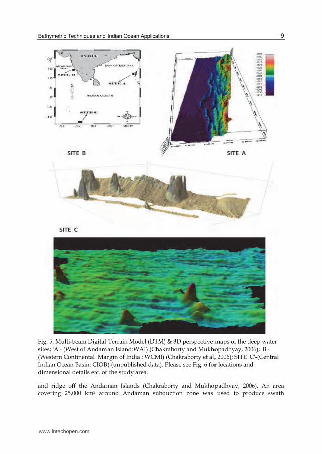
2.1 Bathymetry of shallower areas

Small scale topographic prominences were seen during the echo-sounding surveys, those are formed of algal and/or oolitic limestone on the outer continental shelf off many tropical coasts. Similar features were observed during the course of multi-beam echo-sounding survey on the "Fifty Fathom Flat" off Mumbai, the west coast of India (Nair, 1975). The shelf width off Mumbai is 300 km. The outer 250 km of the shelf, have depth within the 65 to 100m. Small scale features such as pinnacles having heights generally varying from 1-2m, occasionally reaching a maximum height of 8m at some places along with the associations of trough like features. Progressive increase in the relief is observed as one proceeds from shallow to deep waters. In addition to these features, mound shaped protuberances are also varying from 2000-4000m. The height of such mound shape features are varying within the 6-8m. These features are prominently observed beyond the outer shelf of 80-85m, and shelf break in this area occurs at 95m water depth. Single beam bathymetry available on this margin showed reef-like features and large mounds, both made up of aragonite sands (Rao et al, 2003). The dimensions of these features needing detailed multi-beam survey. It is well known that during the Last Glacial Maximum (LGM) (18,000 14C yrs BP), the Glacio-eustatic sea level was at about 120-130 m below the present position (Fairbanks, 1989). Thereafter the sea level started rising largely due to the melting of glacial ice. The carbonate platform measuring about 28000 km2, extending 4 degrees of latitude lies between the 60 to 110m water depths on the outer continental shelf of the northwestern margin of India. Although the platform lies off major rivers such as Narmada and Tapi, it contains <10% terrigenous material. The relic deposits on the carbonate platform are largely carbonate sands. It is interesting to know how carbonates developed when one considers the geographic setting (off major rivers), age of the sediments of the platform, and environmental conditions (intense monsoon) during the early Holocene (Rao & Wagle, 1997). The absence of terrigenous flux on the platform and continued carbonate growth until 7.6 kaBP, implies that the riverine flux either filled the inner shelf or diverted towards the south under the influence of a southwest monsoon current. Therefore, detailed high resolution multi-beam bathymetry survey should be carried out to understand whether this is biohermal or manifestation of physical processes during lower sea levels. This, in-turn helps to identify the factors inhibiting the terrigenous flux on to the platform and processes operative during lowered sea levels. Below, multi-beam bathymetric map of “Fifty Fathom Height” off

www.intechopen.com


7

Tarapur, Mumbai is presented (Fig. 2). The water depth varies from 70-120m having vertical exaggeration of thirty providing the clear indication of small scale reef like features. The data was acquired using EM 1002 multi-beam system installed on-board Coastal Research Vessel (CRV) Sagar Sukti.

Fig. 2. Multi-beam bathymetric map of the "Fifty Fathom Flat" off Mumbai covering distances along northern and southern axes are 28.25 km and 17.75 km respectively.

On the western continental shelf of India, the middle and outer shelf environment, beyond 60 m depth, is uneven and is characterized by the presence of relict carbonate-rich sediments and a variety of limestones. Numerous prominent reefal structures between water depths of 38 and 136 m have been identified, having positive relief, which is believed to be due to the biohermal growth. These reefs occur seaward within the inner and outer shelf transition zone, as significant number of peaks, pinnacles and protuberances of different heights. The height varies from <1 m to 14 m. In shallow environments, often the reefs are buried below 5 - 10 m thick sediments. Bathymetry data of the western continental map is shown, which has also been acquired using EM 1002 system. Depth variation of 60-85m is shown off northern part of the Goa. Small-scale structures as discussed are prominently seen in the figure (Fig. 3) covering 197 km2 area are presented with a vertical exaggeration of 10. Progressive narrowing of the shelf is observed in the western continental shelf. It is around 60m wide off Goa, and shelf break occurring at 130m water depth. Terrace like features are observed here, however, such features are not so prominent than the off Mumbai area.

Quasim & Nair (1978) discovered a living coral bank at 80m water depth, about 100km from the coast off Malpe (Karnataka state), west coast of India and named it as Gaveshani bank. The bank has a height of 42m, length of 2km and width of 1.66 km having area of 3.00 km2 (Figure 4). Walls of this bank rise steeply from the seafloor. Sediments collected by grabs from the seafloor around the bank were silty sand, predominantly carbonate, consisting of shells of foraminifera, fragments of mollusks and corals. The radio carbon age of the sediments and rocks from the outer continental shelf is between the 9000 and 11000 yr. This period corresponds to Holocene when sea level began to rise or when it was in transgressive

www.intechopen.com


8

state. Living corals were acquired from the bank and five major species were identified. Coral growth in the area might have started in the Pleistocene when sea level was low.

Fig. 3. Multi-beam bathymetry map showing small scale features off Goa covering distances along northern and southern axes are 17.50 km and 13.30 km respectively.

2.2 Bathymetry of deeper areas

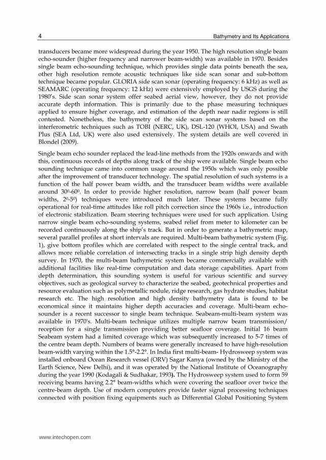
In (Fig. 5) deep water areas from three Indian Ocean regions are presented. Locations of the present interest include: West of the Andaman Island (WAI), Western Continental Margin of India (WCMI) and Central Indian Ocean Basin (CIOB). The topographic data was collected using multi-beam echo sounder Hydrosweep system. Quantitative estimation of roughness parameters from a range of seafloor areas may help to understand the genetic linkages among the area seafloor features (Chakraborty et. al, 2007). Bathymetric data from the Andaman subduction zone in the Bay of Bengal (site A) consists of plain, trench, slope

Fig. 4. Multi-beam map of the coral bank- Gaveshani bank covering distances along northern and southern axes are 2.40 km and 1.40 km respectively.

www.intechopen.com


9

Fig. 5. Multi-beam Digital Terrain Model (DTM) & 3D perspective maps of the deep water

sites; 'A'- (West of Andaman Island:WAI) (Chakraborty and Mukhopadhyay, 2006); 'B'-

(Western Continental Margin of India : WCMI) (Chakraborty et al, 2006); SITE 'C'-(Central

Indian Ocean Basin: CIOB) (unpublished data). Please see Fig. 6 for locations and

dimensional details etc. of the study area.

and ridge off the Andaman Islands (Chakraborty and Mukhopadhyay, 2006). An area covering 25,000 km2 around Andaman subduction zone was used to produce swath

www.intechopen.com


10

bathymetric map (Fig. 5). In this area the heavier Indian plate is shoving below the lighter continental Eurasian plate and causes the subduction morphology and associated structural features. The depth values were found to be varying between the 3600 m (western end of the trench side) to ridge areas (towards the Island side) having seafloor depth of 1000 m. In this region, the bathymetric grid cell size is taken to be 150 m, and the bathymetry map is presented. Data along three survey tracks (A to C) (Fig. 6) across the trench and other areas were collected to constrain exact physiographic profiles of the trench and the ridge. About 20,500 km2 area was surveyed off the central west coast of India (WCMI) (Chakraborty et. al, 2006 & Mukhopadhyay et al, 2008). WCMI data (site B) was acquired between the Karwar and the Kasargod. As mentioned, the seafloor topography in the area varies from nearly flat continental shelf to lower slopes (Fig. 6). The slope morphology appears to have modified by the presence of physiographic highs of varied dimensions and slump related features. In site B (WCMI) depth varies from shallow water (~ 64 m) to deep water (~2200 m). In order to obtain evenly spaced data, the raw data were first gridded. In site B, 100 m was found to be a suitable grid cell size, later on three bathymetric profiles namely D, E, and F covering outer shelf, Mid- Shelf Basement Ridge upper slope, and Prathap ridge of the basin were extracted respectively. In CIOB (site C), the gridding was carried out using suitable grid cell size of 200 m. Bathymetric maps (Fig. 5) were prepared having water depth varying between 4200 – 5800 m and later on five bathymetric profiles were extracted G-K. Of these, three E-W profiles (G-I) are situated in the northern and southern end. Other two N-S profiles (J and K) are situated along west and eastern end. It has been observed that, the western region of the site C is comparatively shallower than the eastern side and the seafloor morphology varies from medium to large scale and has E-W trending in the central part of the area. A chain of seamounts trending along N-S direction was also observed in the extreme eastern region of the study area. Also, few seamounts were observed in the south-west section of the map. The five depth profiles (G, H, I, J and K) from grid data are studied for roughness information from north central, south, east, and west part of the survey area respectively.

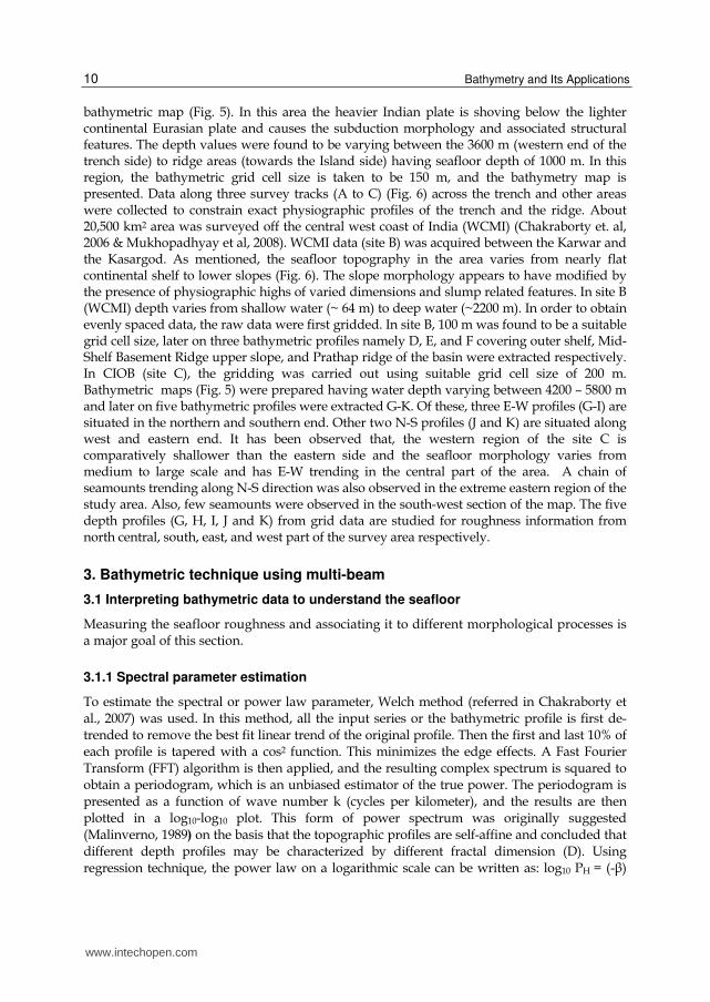
3. Bathymetric technique using multi-beam

3.1 Interpreting bathymetric data to understand the seafloor

Measuring the seafloor roughness and associating it to different morphological processes is a major goal of this section.

3.1.1 Spectral parameter estimation

To estimate the spectral or power law parameter, Welch method (referred in Chakraborty et al., 2007) was used. In this method, all the input series or the bathymetric profile is first de-trended to remove the best fit linear trend of the original profile. Then the first and last 10% of each profile is tapered with a cos2 function. This minimizes the edge effects. A Fast Fourier Transform (FFT) algorithm is then applied, and the resulting complex spectrum is squared to obtain a periodogram, which is an unbiased estimator of the true power. The periodogram is presented as a function of wave number k (cycles per kilometer), and the results are then plotted in a log10-log10 plot. This form of power spectrum was originally suggested (Malinverno, 1989) on the basis that the topographic profiles are self-affine and concluded that different depth profiles may be characterized by different fractal dimension (D). Using regression technique, the power law on a logarithmic scale can be written as: log10 PH = (-β)

www.intechopen.com


11

log10 k + log10 c. Comparing this equation with the straight-line equation reveals that ‘β’ corresponds to the slope of a straight line fitted to the periodogram and ‘c’ corresponds to the intercept. At this stage the straight regression line fitting is done for the entire range of log10

(wave number) of the periodogram. The detailed post processing activity is shown (Fig. 7).

Fig. 6. Contour maps and chosen tracks for data analyses (adapted from Chakraborty et al., 2007). Sites; 'A'- (West of Andaman Island :WAI) (total area: 25000 km2, maximum: 3600m and minimum depth: 1000m); 'B'- (Western Continental Margin of India : WCMI) (total area: 25500 km2, maximum: 2200m and minimum depth: 64m); 'C' - (Central Indian Ocean Basin: CIOB) (total area: 22000 km2, maximum: 5800m and minimum depth: 4200m).

www.intechopen.com


12

Fig. 7. Flow chart provides data processing and analyses steps (adapted from Chakraborty et al, 2007).

3.1.2 Amplitude parameter

The second parameter that is used to characterize the roughness of the profile is an amplitude parameter (S). A robust estimate is the median of the absolute deviation (MAD) from the sample median is given below:

MAD = median | z(x) - MEDIAN [Δz(x)] | (1)

where Δz(x) is the first differences of the depth series z(x). An estimate of 'S' from MAD is defined as:

S = 1.4826 * MAD (2)

www.intechopen.com


13

Segmentation carried out to nine long profiles from three different physiographic provinces

give 35 segments. Three profiles (A, B and C) for site A of WAI region provide 12 segments

(Fig. 8). Our algorithm offers no segmentation to profile A from deeper section of this area

having depth range higher than the 3000 m and 225 km of profile length towards the

sedimentary provinces of trench side (Fig.5). Four segments were obtained for profile B

which lies between the sedimentary trench and ridge area having an undulating seafloor at

similar depth range. For profile C from relatively shallower depth section of ridge area

provides seven segments at depth range 2000 -2400 m. Similarly, for site B from WCMI the

profile D from shallower shelf (depth within the 100 m) presents only two segments. Eight

topographic segments were obtained for profile E from the Mid-Shelf Basement Ridge.

Distinctly different segments for flank parts (E4 and E6) along the bathymetric high E5 of

the profile E are seen (Fig. 8). However, four segments obtained for deeper section of the

profile are from sedimentary areas of the Prathap Ridge (conical features of the heights in

Fig. 5). For this profile F, two highs having significantly different heights, are distinctly

segmented. Overall, fourteen segments are made for this part (site B) of the physiographic

provinces. For CIOB (site C), five profiles provide only nine segments from the deeper part

of the seafloor (~ 5000 m depth) (Figure: 8). From this basinal part of the seafloor, west to

east profiles G and H from the northern and middle part of the area do not offer any

segment. Interestingly, remaining depth profile (I) from E-W direction provides four

segments. Profiles J from western and K from eastern end provide two and one segments

respectively. Once segmentation of the profiles are carried out, the estimation of power law

exponent (β) for segmented profiles are important for calculation of fractal dimension. The

bathymetric profiles extracted from the three different sites viz. A, B and C have sampling

intervals of 150 m, 100 m and 200 m respectively. Hence, the extent of the periodogram on

the higher wave number side in terms of log10(wave number) is limited to 0.50, 0.65 and 0.40

for site A, B and C respectively i.e., the true drop in power occurs somewhere between the

wavelengths ~20 to ~0.2 km for Hydrosweep system operating at 15.5 kHz frequency (Fig.

8). Hence suitable limits are applied to the periodograms for curve fitting in order to

estimate the spectral parameters (power law). In Fig. 8, power spectral density versus wave

number plots for segmented sections (C4, E2, and J1) of the profiles C, E and J are presented

respectively as an example.

3.1.3 Fine scale analyses using ‘β’ and ‘S’ parameters

Overall, the ‘’ values are always negative and having large magnitudes, representing

terrains which are relatively rough at large and smooth at smaller scales. Conversely, lower

magnitudes of the ‘’ parameter represent terrains which are smoother at large scales than at

small scales. The scatter diagram between the power spectral exponent () and amplitude

(S) parameters offer interesting results (Fig. 8). Overall variations in the roughness of these

study areas may group in distinct clusters. For WAI physiographic provinces, the seafloor

along the profile from sedimentary provinces of the trench side of site A possesses β and S

values: 0.93 and 3.55 respectively. Profile A from sedimentary provinces of the trench side

possesses β and S values: 0.93 and 3.55 respectively. As mentioned, high β corresponds to

rough seafloor, while S quantifies amplitude (overall energy) of an area. For example,

profiles having similar β but higher S will correspond to rough profile. Diagram (Fig. 8a)

www.intechopen.com


14

for this physiographic province indicates an isolated point (A1) for a rough seafloor from

trench side. However, four segmented profiles (B1– B4) between the trench and ridge side

provide (β= -1.87 and S= 6.50), (β= -1.64 and S= 10.20), (β= -2.00 and S= 8.86) and (β= -

1.77 and S= 13.90) respectively. Similarly, for seven segmented sections of profile C from

adjacent ridge area from Andaman Island provide variations of spectral parameter (β)

value between (2.19 to 3.02) and amplitude parameter S value (15.20 to 3.20). A critical

analysis of these results indicate significantly lower β in comparison with the segments of

the profile A i.e., smooth seafloor than the segments from the profile B & C. No clear cut

cluster formation is seen in WAI region. Moderately to higher amplitude (S) parameters for

profiles B&C data and relatively higher β value for profile A is indicative of higher large

scale (B&C) and small scale (A) seafloor roughness respectively.

For site B of the WCMI, estimated ‘’ and ‘S’ values of fourteen segmented sections are

found to vary between (-3.56 and -0.90), and (0.24 and 22.28) respectively. The scatter

diagram between the power spectral exponent () and amplitude (S) parameters offer

interesting results (Fig. 8). The overall roughness observed in the study area groups in two

distinct clusters. Cluster one includes segments from structural rises like: E6 (flank related to

Mid-Shelf Basin Ridge), F1 (highs related to the Prathap Ridge) and F3 (S=22.28 consisting of

two to Mid-Shelf Basin Ridge), F1 (highs related to the Prathap Ridge) and F3 (S=22.28

consisting of two small closely associated highs and not included in Fig. 8). These areas

show high S and low to medium values, which suggest large scale seafloor roughness. In

contrast to this, another cluster comprises the remainder of the areas, including a gently

sloping outer shelf and part of the western shelf margin basins. The seafloor here shows low

S and moderate to higher value, suggesting dominantly small-scale undulations. A

comparison of the clustering of the structural rises with that of the outer continental shelf

and basin regions (Fig. 8) indicate differences in their mode of origin (volcanic and plutonic,

respectively). For example, the Mid-Shelf Basement Ridge and the Prathap Ridge are

believed to have been formed by emplacement of volcanic material during the separation of

India and Madagascar in mid-Cretaceous times. Detailed tectonic and other aspects of these

areas in terms of clustering are well covered in Chakraborty et al (2006).

The analyses based on the spectral and amplitude parameters in the study site C (CIOB)

has a seafloor depth vary between 4200 m and 6000 m depth. The estimated ‘’ and ‘S’ values of the E-W profiles (G, H and I) are found to be varying between (-1.14 and -2.70)

and (7.44 and 4.87) respectively (Fig. 8). Also ‘’ and ‘S’ values of N-S profiles are found to vary between (-1.70 and –2.083) and (13.33 and 12.75) respectively. If we remove data points related to the southernmost E-W segmented sections (I2, I3 and I4) of the profile I, the β parameter becomes comparable (-1.70 and -2.10) with N-S profiles (J and K), though, the amplitude parameter (S) are higher for N-S oriented profiles varying between (12.75 and 13.49) than the E-W profiles (4.9 and 7.9). Though we observe most of the profiles /

segmented sections are similar, as far as is concerned, however, show clear-cut existence of two clusters due to variation in amplitude parameter. The amplitude parameters show difference between the E-W and N-S profiles i.e., the amplitude (S) for N-S oriented

profiles are higher than the E-W profiles (Kodagali & Sudhakar, 1993). For similar values towards the E-W and N-S direction with higher amplitude for N-S profiles than the E-W indicate dominant large scale roughness for N-S profiles whereas E-W profiles

www.intechopen.com


15

indicate dominant small scale roughness. This fact is prominently clear in the report (see Fig. 5) (Malinverno, 1990).

3.2 Beam-forming technique to generate multi-beam data

In a multi-narrow beam system, geometrically a cross fan beam is created using two hull

mounted linear/arc transducer arrays at right angles to each other. A narrow beam is

produced in a direction which is perpendicular to the transducer's short axis. In general, the

arrays are designed using a number of identical transducer elements which are equally

spaced and driven individually. An assumption of an array which is kept at the origin of the

co-ordinate system in a xy- plane, is made here. The separation between the elements is

equivalent to 0.5 λ, where λ is assumed to design wavelength of the transducer array. The

farfield pattern for a linear array is given by (Chakraborty, 1986):

The array factor f (θ, φ ) is presented by as:

|F (θ, φ ) | = |f (θ, φ ) |Element pattern| (3)

f (θ, φ ) =n

nn=1

A exp (j k rm. R)

where An is the complex excitation coefficient, which is assumed to be unity and k= 2 / λ

and n is the number of array elements. For above linear array: rn= dn i, where dn is the

element separation from the origin, and i is the unit vector along the x-axis. The polar unit

vector R can be expressed as:

R= (Sin θ Cos φ) i

The array factor for a linear array can be written as:

f (θ, φ ) = n

nn=1

A exp (j k dn Sin θ Cos φ)

The amount of phase delay required between the transmitting elements to steer the beam along the specified direction (θo, φ o) may be expressed as:

n =dn. k (Sin θ0 Cos φ0) i

The above term is to be applied to the far-field pattern of a uniformly excited linear array of the additive type. The farfield beam pattern in the final form is rewritten as:

f(θ, φ) = n

nn=1

A exp j {(k dn Sin θ Cos φ) - (dn. k Sin θ0 Cos φ0)} (4)

In equation (3)

Element pattern = Sin ( l Sin θ Sin φ) / (Sin θ Sin φ) (5)

where l is the length of the element and is equivalent to the 3.0 λ. The final expression for the

vertical farfield pattern can be obtained by substituting equation (4) and equation (5) in

www.intechopen.com


16

equation (3). The farfield pattern of a multi-beam array of 40 elements is shown (Figure 9).

The half power beam widths slowly increase: 3.0 to 3.6o as the beam steering angles

increases. The computed half power beam-widths are generally narrow and are useful for

high resolution bathymetric applications. Sidelobe 1evels around -13 dB for all the

incidence angles are also seen. Sidelobes are also a concern in echo-sounding. There are

certain techniques for suppression of the sidelobes, which significantly affect the

performance of the array. For multibeam applications where many beams for different

look directions are forming at a particular instant of time, sidelobes are assumed to be

suppressed below -25 dB. This is necessary to avoid interference between the sidelobes

and the main beam of the other directions. These sidelobe suppressions are accomplished

by using Dolph-Chebychev window methods. Apart from that, sidelobe levels cannot be

suppressed extensively beyond certain levels. Because it increases the width of the main

beam and thus decreases the resolution. So suppressed sidelobe beam patterns around -25

dB for multibeam transducer array are acceptable as considered by echo-sounder

designers (de Moustier, 1993).

Fig. 8. Segmentation of the representative track lines and power law fitted straight lines and scatter plot of three geological provinces (adapted from Chakraborty et al., 2007).

www.intechopen.com


17

Fig. 9. Beam pattern for a 40- element linear array at different directions (adapted from Nair and Chakraborty, 1997).

3.2.1 Importance of sound velocity and other parameters for bathymetry

Using array transducers for beam-forming purposes the preformed beam directions are

dependent on the used acoustic wavelength which is a function of the sound speed C, i.e

λ=C/f, where C is in m/s and f is in Hz. For any changes in the sound velocity (C), λ will

change. The sound speed is dependent on temperature, salinity and pressure (depth). Chen

& Millero (1977) had proposed an expression to compute the sound velocity. Sound speed

changes occur mostly due to temperature and salinity variations. Hence, variations of ƛ

value with the variations of sound velocity, will change the half power beam-width of the

array and also shift the beam direction. Sound speed changes of 6.6 percent are possible for

an echo-sounding system operating at arctic and Tropical waters (temperature difference of

30°C). Similarly for λ variation of 3.3 percent, a beam rotation of 0 to 45° will introduce an

error amount of 1.9° for a narrow beam of 2° beam-width. Also for swath bathymetry

application, the variation of sound speed over the entire water column must be considered.

The angle of arrival of the different beam is affected due to the refraction effect which is

dominant, for the outer beams of the array system. In order to correct: the refraction error in

echo-sounding systems, computation of the sound system should be performed by

integrating the sound speed profile from the depth of the array to the bottom. The harmonic

mean of the sound, speed is preferred over the average sound speed (Maul & Bishop, 1970

referred in Nair and Chakraborty, 1997). The multi-beam echo-sounder systems acquire

bathymetry data along with other data can be used in scientific studies. As observed most of

the multi-beam data is occasionally recorded with errors (de Moustier and Kleinrock, 1986),

are either geometrical or refraction in nature. But to obtain a map that can be used either for

navigation or scientific purposes, it is necessary that the data is error free. As per IHO

standards the refraction affected data in shallow waters include uncertainties from

navigation point of view. Also, to use in scientific applications it is vital to eliminate these

errors from the bathymetry data. The refraction error influences the slant ranged beams and

can be easily identified as the swath shape deviate in creating artificial features known as

refraction artifacts.

www.intechopen.com


18

For development of echo-sounding devices, certain parameters are of paramount importance to obtain optimum signal to noise ratio. Source level i.e. the transmitted power

measured at 1m from the transmitting array is an important parameter. Similarly, transmission loss in the medium is also compensated at TVG (Time Varied Gain) module of

the receiver. Apart from that, the noise level is also another important issue for the designer of the multibeam system. The noise level parameter is dictated by the location of the array in

the hull. i.e., array should be kept in the forward part of the ship's hull, which is closest to the central line. The machinery noise is minimum in this area of the ship. The positioning of

the array should also be decided based upon the ship's movement due to roll and pitch. Therefore, the array should be maintained submerged throughout the ship's movement. The

major signal processing event which is known as beam-forming takes place at the receiver end of the array. The received signals are pre-amplified and each channel signal (array

element) undergoes a correction for TVG loss in the correction unit and then beam forming techniques are applied to obtain multiple beams using predetermined delays for different

directions. The theoretical backgrounds of the multi-beam signal processing methods have already been mentioned. The beam-formed waveforms are tracked at a bottom echo module

for different preformed beam directions in order to determine the depth.

3.2.2 High resolution beam-forming

In multibeam sounding system, the delay-sum method (the method mentioned above) is used to obtain the beam-formed output in different directions. The size of the transducer array is a function of the beam width i.e., the spatial resolution of the system. At 15 kHz design frequency for a beam width of 2°, the approximate size of the transducer array has to be around 3 meters, which is relatively bulky. So a study is important to examine the effect of various methods of beam-forming which require a smaller array size by using increased signal processing alternatives to the dry end of the multibeam system. These techniques are the 'Maximum Likelihood Method' (MLM), and 'Maximum Entropy Method' (MEM) (Jantti, 1989 & Chakraborty &: Schenke, 1994).

The situation is more complicated when multibeam systems are operated over seamounts,

slopes or ridge areas. The multiple sources of interference arrivals from different directions are

well known. This condition significantly affects the map resolution so that an assumption of

coherent and incoherent source arrival conditions is introduced to study the performance of

the high resolution techniques. In Fig. 10, we present high resolution (MLM) beam patterns for

incoherent and coherent sources. We assume that the sources are separated at 2° and 8° for

different input signal to noise ratio. We observe that for closely placed sources (2°), the sources

are unresolvable for coherent and incoherent sources. For large source separations of 8° the

sources are resolvable for both the source conditions. The number of elements was chosen to

be 16 which is one-fourth of the conventional array size used for multibeam systems. This

techniques are affected due to the low signal to noise ratio conditions, and therefore needs to

be studied using different algorithms such as ESPRIT, MUSIC, etc (Jantti, 1989). The high

resolution beam-forming technique must also consider its use towards the real time

application. It is unlikely that a single algorithm will satisfy all the necessary conditions to

generate noise free bathymetry output. Development of a decision making network should be

the next stage of development. This network will find suitable high resolution algorithms in

real time and would be useful for multi-beam applications.

www.intechopen.com


19

Fig. 10. Multi-beam High-Resolution beam patterns (MLM: Maximum Likelihood Method)

for 16- element array. The sources are incoherent and coherent types of different signal

strengths (adapted from Nair and Chakraborty, 1997).

4. Bathymetry and backscatter data

However, bathymetry only provides the shape of the seafloor features and depends on the resolution of the sounding system. To characterize the nature of the seafloor surveyed, studies of signal waveforms and their variations must be made, i.e. understanding of the backscatter signal is essential. Using the capabilities of multibeam system to provide backscatter signal from different incidence angle, modeling can be performed for seabed classification.

4.1 Angular backscatter data & quantitative seabed roughness

Multibeam systems are useful to derive angular dependent backscatter function of the seafloor. Besides bathymetry, different types of seafloor can be differentiated based on the backscatter values obtained at different incidence angle by the multibeam echo-sounder.

www.intechopen.com


20

The aim of such study is to determine whether bottom types can be determined using angular backscatter functions. In addition, determination of the influence of the sea water-floor interface or sediment volume roughness parameter is possible. The Multibeam technique is particularly suitable to the task of deriving angular dependence of seafloor acoustic backscatter because it provides both high resolutions related to such measurements and bathymetry. Though it is difficult to calibrate the backscatter data, quantitative estimation may be made even for the relative values. The use of composite roughness theory (Jackson et al, 1986) is being made to obtain seafloor parameters. In the composite roughness theory, Helmholtz –Kirchhoff’s interface scattering conditions and perturbation conditions were used including the volume scattering parameters. Extensive modeling studies have been carried out to use angular backscatter data to obtain quantitative roughness and sediment type parameters. A significant amount of work is carried out to obtain quantitative seafloor roughness parameters using bathymetric system such as multi-beam and single beam system (de Moustier & Alexandrou, 1991). The main challenge lies with this application is connected with the calibration, and work is still in progress to make a bathymetric system to obtain quantitative roughness parameters. An example of the use of inversion modeling from nodule bearing seafloor is provided (Fig. 11). The interface roughness and sediment volume parameters are estimated using the composite roughness theory (Chakraborty et al, 2003) from CIOB.

Fig. 11. Measured (dotted line in bold) and model backscatter strength (decibels) due to sea-floor-interface roughness (crossed line) and sediment volume roughness overlying sea-floor interface roughness (dashed line) versus incidence angle for four study areas (adapted from Chakraborty et al, 2003).

www.intechopen.com


21

4.2 Seafloor backscatter image data

The side scan modifications to the multibeam system are also a popular technique. The raw side scan data requires significant image enhancements. Extensive work on image enhancements techniques has been carried out for side scan systems such as GLORIA and SEAMARC (Mitchell & Somers, 1994). Large scale implementation of these techniques is made for multibeam systems. Application of multi-beam bathymetric data provides interesting seafloor features. Besides obtaining bathymetric data for seabed characterization backscatter data is also important. However, use of raw multi-beam backscatter image data is limited due to the presence of inherent artifacts. Generally, angular backscatter strength data show higher values towards the normal incidence angles especially for smooth seafloor compared to outer-beam angles. Therefore, off-line corrections are essential to compensate outer-beam backscatter strength data in such a way that the effect of angular backscatter strength is removed. Moreover the effect of on line gain functions employed to the multi-beam is also to be removed apart from the effect of the large scale seafloor slope along and across track directions. These techniques employed to backscatter strengths data of the multi-beam system provides a normalized image of the seafloor suitable for studying sediment lithology.

EM 1002 multi-beam echo-sounding system installed onboard CRV Sagar Sukti has 111 pre-formed beams i.e., recording 111 depth values for a single ping. In addition to the depth, the system also provides quantitative seafloor-backscatter data, which is utilized to generate normalized backscatter imagery for the study of spatial distribution of fine scale seafloor roughness and textural parameter. Originally during the time of acquisition and consequent storage, individual angular backscatter strength data is corrected for number of losses and changes such as Time Varied Gain (TVG), i.e., propagation losses, predicted beam patterns and for the ensonified area (with the simplifying assumptions of a flat seafloor and Lambertian scattering). This data then gets recorded in a packet format called datagram stored for every ping. A very brief discussion of the developed algorithm named as PROBASI (PROcessing BAckscatter SIgnal) II applied to raw backscatter data of the EM 1002 multi-beam system in order to obtain normalized backscatter image data.

In EM 1002 system online amplifier gain correction is accomplished by applying mean backscattering coefficients such as BSN and BSO applied at 0º and at crossover incidence angles (normally 25º) respectively. Consequently the raw backscatter intensities recorded in the raw (*.all) files are corrected during data acquisition employing Lambert’s law (Simrad Model). However, for lower incidence angles (within the 0-25º) the gain settings in the electronics require a reasonably smooth gain with incidence angle i.e., the gain between BSN

and BSo changes linearly. The sample amplitudes are also corrected suitably incorporating transmitted source level and transducer receiver sensitivity. Further, sonar image amplitudes, though corrected online, needs further improvement to generate normalized images for the seafloor area. This is especially needed for incidence beam angles within the +/10º angles (to remove routine artifacts in the raw backscatter data near normal incidence angles) (Fig. 12). Hence, post processing is essential to be carried out even for moderately rough seafloor. In addition to the artifacts close to normal incidence beams, the EM 1002 multi-beam data show some residual amplitude due to beam pattern effect, and thus real time system algorithm is unable to compensate such routine situations. As we know that, the EM1002 multi-beam echo-sounder system automatically carries out considerable amount of processing on raw backscatter intensities. Even then, the data show some residuals, which are required to be corrected before further studies. These fluctuations may be due to: Seabed

www.intechopen.com


22

Angular Response and Transducer Beam Pattern Effects. Four basic corrections are made during the application of the PROBASI II software: data extraction and geometric corrections, heading correction, position correction, bathymetry slope correction and Lambert’s law removal. In short the entire developmental activities are divided into four modules adopted through following procedure (Fernandes & Chakraborty 2009):

Fig. 12. Flow diagram of multi-beam processing algorithm (PROBASI II), and HPF & LPF

are the high pass filter & low pass filter respectively.

www.intechopen.com


23

Module-I: This extracts data from seabed image, raw range and beam angle, depth, attitude and position datagrams (EM Datagrams Manual). The module applies heading, position, slope correction on data and eliminates the effect of Simrad Model from data.

Module-II: It employs a coarse method. The module filters out maximum residuals or spikes in the backscatter strengths. This improves the image by 20% over the raw backscatter image.

Module-III: This module utilizes iterative beam pattern removal method in a finer sense. Since the coarse method does the maximum job of removing center beam and beam pattern effects. Still to some extent small beam pattern residuals remain in the data. The employed fine method removes such residuals more prominently.

Module-IV: The noise is an influencing factor on the quality of backscatter strengths. Since this type of data directly deals with the signal strength, sometimes the data gets recorded along with the noise occurring at the face of the transducer. Therefore, use of the filters becomes necessary. This module uses a combination of high pass and low pass filters.

4.3 Use of multi-beam bathymetry and backscatter data for pockmark studies

In this section we have presented a study example from western continental margin of India

where backscatter image and bathymetric data is applied in a combined manner to generate

a better picture of the proxies related to non-living resources such as pockmark (Dandapath

et. al, 2010 and references therein). The pockmarks are potentially important for studies of

marine resources and environments because of their relationship with venting of gas or

other fluids generated by biogenic or thermogenic processes. Multibeam echo-sounders are

potentially useful for locating and mapping these pockmarks. The presence of fluid escape

features like seafloor pockmarks was first introduced by King & MacLean (1970). Generally,

these are either hemispherical or disc shaped seafloor depressions having steep sides and

flat floors. Very often, pockmarks exist in the continental margins (Hovland & Judd, 1988).

In plan-view, these are usually circular, elliptical or elongated, and may be composite in

shape. Present study area stretches over 105 km2 offshore Goa along WCMI (Fig. 13), in

water depths ranging from 145 m in the northeast to 330min the southwest. The average

slope of the study area is 0.900, whereas the slope towards the shallower depth is 0.610, and

towards the deeper side this slope changes over to 1.680. Rao et al., (1994) have reported that

the recent clay-rich mud overlies the inner part of this slope area while relict sand is

abundant in the outer slope area. In this work, using multibeam data, set of pockmarks were

observed close to NNW-SSE trending fault zone. The margin is believed to have been

formed in two phases in geological past (Mukhopadhyay et al., 2008). Interestingly, these

pockmarks (total: 112) are observed nearly 50 km away from a BSR zone (Rao et al., 2003)

marked in the Fig. (13b). Acoustic backscatter strength of the area ranges from -26 to -57 dB.

Such backscatter variability is related to the seafloor slope, sediment type and relief

(Blondel, 2009). Backscattering strengths at different water depth for each individual

pockmark centre. In the deeper water (>210 m), many pockmarks show high backscatters

centrally (-27 to -40 dB). Towards the west in deeper water, the seafloor has strong

backscatter (-35 dB) suggesting coarser grained sediment at the seafloor because of increased

acoustic impedance, and roughness-related scattering from coarse sediment. In shallow

water (<210 m) where seabed gradients are gentle, normally backscatter strength is low. The

www.intechopen.com


24

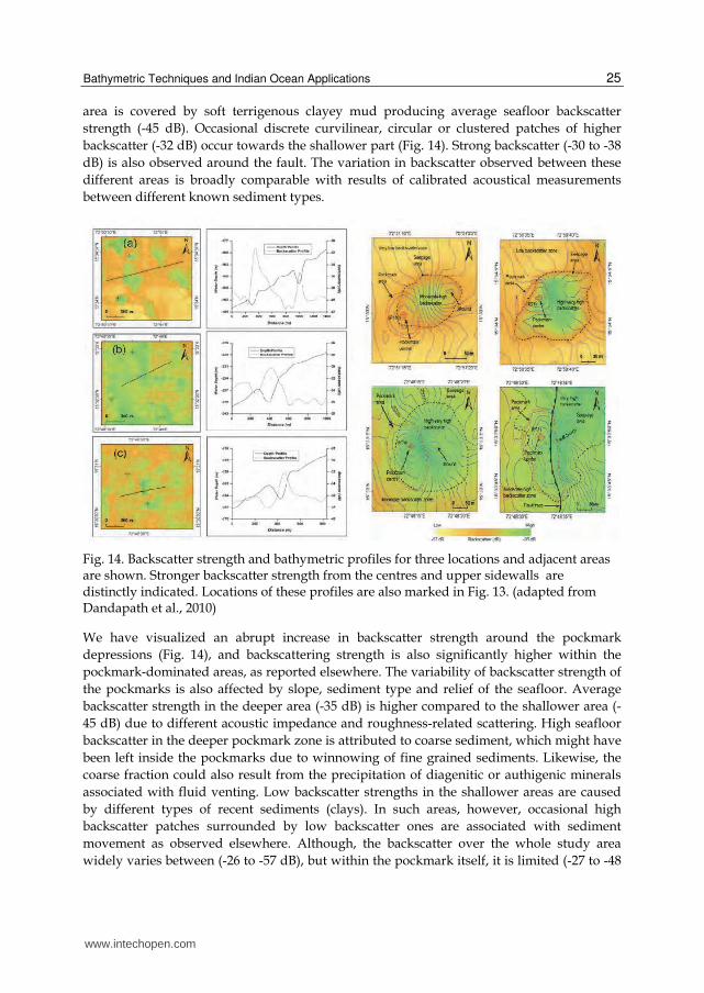
Fig. 13. (a) Location of study area. Red highlighted lines and grey shade indicate the identified bottom simulating reflectors. MSBR refers to Mid-Shelf Basement Ridge, and WCF indicate West Coast Fault. (b) Backscatter map of the study area showing isobaths with an interval of 20 m depth. Pockmarks are indicated by crossed circles. Black, blue and red circles with cross marking represent circular, elliptical and elongated pockmarks, respectively. Dashed lines indicate location of identified faults. Solid black lines represent location of the corresponding profiles for Fig 14. (adapted from Dandapath et al, 2010).

www.intechopen.com


25

area is covered by soft terrigenous clayey mud producing average seafloor backscatter

strength (-45 dB). Occasional discrete curvilinear, circular or clustered patches of higher

backscatter (-32 dB) occur towards the shallower part (Fig. 14). Strong backscatter (-30 to -38

dB) is also observed around the fault. The variation in backscatter observed between these

different areas is broadly comparable with results of calibrated acoustical measurements

between different known sediment types.

Fig. 14. Backscatter strength and bathymetric profiles for three locations and adjacent areas are shown. Stronger backscatter strength from the centres and upper sidewalls are distinctly indicated. Locations of these profiles are also marked in Fig. 13. (adapted from Dandapath et al., 2010)

We have visualized an abrupt increase in backscatter strength around the pockmark

depressions (Fig. 14), and backscattering strength is also significantly higher within the

pockmark-dominated areas, as reported elsewhere. The variability of backscatter strength of

the pockmarks is also affected by slope, sediment type and relief of the seafloor. Average

backscatter strength in the deeper area (-35 dB) is higher compared to the shallower area (-

45 dB) due to different acoustic impedance and roughness-related scattering. High seafloor

backscatter in the deeper pockmark zone is attributed to coarse sediment, which might have

been left inside the pockmarks due to winnowing of fine grained sediments. Likewise, the

coarse fraction could also result from the precipitation of diagenitic or authigenic minerals

associated with fluid venting. Low backscatter strengths in the shallower areas are caused

by different types of recent sediments (clays). In such areas, however, occasional high

backscatter patches surrounded by low backscatter ones are associated with sediment

movement as observed elsewhere. Although, the backscatter over the whole study area

widely varies between (-26 to -57 dB), but within the pockmark itself, it is limited (-27 to -48

www.intechopen.com


26

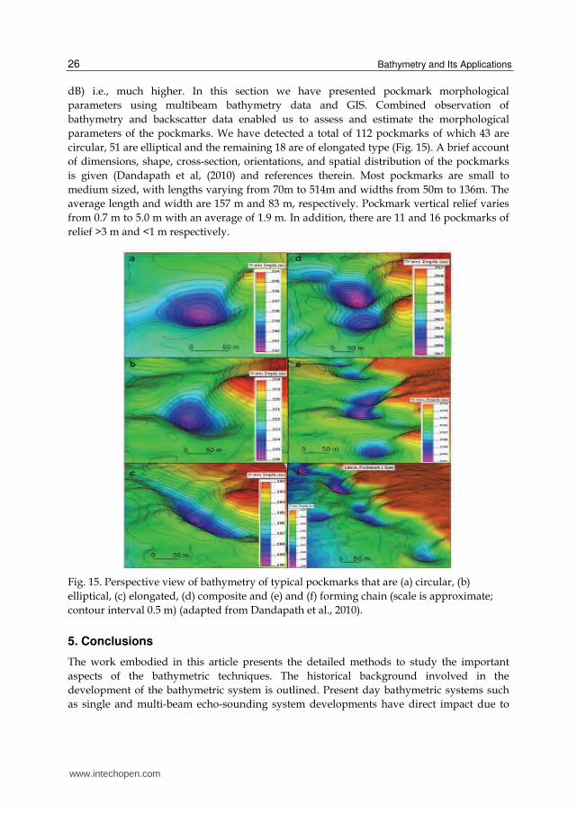
dB) i.e., much higher. In this section we have presented pockmark morphological

parameters using multibeam bathymetry data and GIS. Combined observation of

bathymetry and backscatter data enabled us to assess and estimate the morphological

parameters of the pockmarks. We have detected a total of 112 pockmarks of which 43 are

circular, 51 are elliptical and the remaining 18 are of elongated type (Fig. 15). A brief account

of dimensions, shape, cross-section, orientations, and spatial distribution of the pockmarks

is given (Dandapath et al, (2010) and references therein. Most pockmarks are small to

medium sized, with lengths varying from 70m to 514m and widths from 50m to 136m. The

average length and width are 157 m and 83 m, respectively. Pockmark vertical relief varies

from 0.7 m to 5.0 m with an average of 1.9 m. In addition, there are 11 and 16 pockmarks of

relief >3 m and <1 m respectively.

Fig. 15. Perspective view of bathymetry of typical pockmarks that are (a) circular, (b)

elliptical, (c) elongated, (d) composite and (e) and (f) forming chain (scale is approximate;

contour interval 0.5 m) (adapted from Dandapath et al., 2010).

5. Conclusions

The work embodied in this article presents the detailed methods to study the important

aspects of the bathymetric techniques. The historical background involved in the

development of the bathymetric system is outlined. Present day bathymetric systems such

as single and multi-beam echo-sounding system developments have direct impact due to

www.intechopen.com


27

current technology level. For example: the wet end of the system i.e., transducer is

developed significantly due to the material development taken place in last two decades.

Moreover, development of computer technology allows faster beam-forming and associated

signal processing techniques to work in real time. The involvement of GIS (Geographical

Information System) in bathymetric mapping also has contributed superbly.

We have presented shallow water multi-beam bathymetric data from three geological

important areas of the western continental shelf of India. The acquired data, and subsequent

processed 3D output from three different environments visualizes the level of the

technology to understand the earth related subject. The qualitative description of the

seafloor processes along with the analyses presented here from “Fifty-Fathom Height” off

Mumbai, northern part of Goa, and coral bank off Malpe generate significant interest. The

numerical technique such as spectral methods employed to the bathymetric data of the

deeper part of the western continental margins of India such as: western Andaman Island

(WAI), western continental margins of India (WCMI), and central Indian Ocean basin

(CIOB) provide power law parameters. The segmentation of the bathymetric data into linear

form and subsequent estimation of the power law parameters through straight line fittings

techniques have open up a method to analyze the seafloor roughness.

Bathymetry only provides depth data based on the functioning of the bottom tracking

gate for echo-sounding system. The echo-waveform analyses to determine arrival time of

the bottom echo depends on the echo-peak (near nadir beams) or energy values (off nadir

beams). The analyses made on such data for roughness studies have limitations.

Comparatively, use of seafloor backscatter data involves entire seafloor insonified area.

Though, large scale roughness i.e., structural aspects can be estimated using bathymetry,

but, in order to estimate roughness towards the small scale end (cm scale) the power law

curves are needed to be extended over high-frequency end. The backscatter data are

found to be useful when applied to study micro-topographic studies employing Jackson

model (1986). Here, we have adopted similar techniques for multi-beam Hydrosweep

system at CIOB.

Moreover, this work also presented backscatter image processing from pockmark

dominated areas of the western continental margin of India. The technique associates

bathymetry as well as backscatter data to provide pockmark morphology along with

seepage details of the area as an interesting example for non-living resource related studies.

However, no claim for completeness is being made in the present work. Nevertheless many

issues of bathymetric systems are made, yielding a scope for future work on various aspects

of the bathymetric systems. Certain issues such as bathymetry using phase measuring

system (de Moustier, 1993) is not covered here, though, modern multi-beam systems possess

hybrid techniques such as beam-forming as well as phase measuring system. The shallow

water data presented throughout in this work have been acquired using such system e,g.

EM 1002 multibeam system.

6. Acknowledgment

We acknowledge the Director, NIO for his permission to publish this work, and are thankful to Ryan Rundle, visiting student (Master degree) fellow under RISE research scheme and

www.intechopen.com


28

Andrew Menezes for reading this manuscript. We also acknowledge the review of Dr. P. Blondel. We are thankful to the Ministry of Earth Sciences, New Delhi (Government of India) for their support. This is National Institute of Oceanography contribution 5066.

7. References

Blondel, P. (2009). Handbook of Sidescan Sonar, Springer/Praxis, Chichester, UK.

Chen, C.T. & Millero, F.J. (1977). Speed of sound in seawater in high pressure, J. Acoust. Soc.

Am., Vol.62, No. 5, pp. 1129-1135.

Chakraborty, B. (1986). Coaxial circular array: Study of farfield pattern and field frequency

responses. J. Acoust. Soc. Am., Vol.79, No. 4, pp. 1161-1163.

Chakraborty, B. & Schenke, H.W. (1995). Arc arrays: studies of high resolution techniques

for multibeam bathymetric applications. Ultrasonics, Vol. 33, No. 6, pp. 457-461.

Chakraborty, B., Kodagali, V.N. & Baracho, J. (2003). Sea-floor classification using

multibeam echo-sounding angular backscatter data: A real-time approach

employing hybrid neural network architecture. IEEE JOE, Vol. 28, No. 1, pp. 121-

128.

Chakraborty, B., Mukhopadhyay, R., Jauhari, P., Mahale, V.P., Shashikumar, K. & Rajesh, M.

(2006). Fine-scale analysis of shelf slope physiography across the western

continental margin of India. Geo-Mar. Letter, Vol. 26, No. 2, pp. 114-119.

Chakraborty, B. & Mukhopadhyay, R. (2006). Imaging trench-line disruptions: swath

mapping of subduction zone. Currrent Science, Vol. 90, No. 10, (2006), pp. 1418-

1421.

Chakraborty, B., Mahale, V.P., Shashikumar, K. & Srinivas, K. (2007). Quantitative

characteristics of the Indian Ocean seafloor relief using fractal dimension. Indian

Jour. Mar. Sci. (Special Issue on Fractals in Marine Sciences), Vol. 36, No. 2, pp. 152-161.

Dandapath, S., Chakraborty, B., Karisiddaiah, S.M., Menezes, A.A.A., Ranade, G.,

Fernandes, W.A., Naik, D.K. & Prudhvi Raju, K.N. (2010). Morphology of

pockmarks along the western continental margin of India: employing multibeam

bathymetry and backscatter data. Mar. Pet. Geol., Vol. 27, No.10, pp. 2107-2117.

de Moustier, C. & Kleinrock M. C. (1986). Bathymetry artifacts in the Sea Beam data: How to

recognize them and what causes them. J. Geophys. Res. Vol. 91, No. B3, pp. 3407-

3424.

de Moustier, C. & Alexandrou, D. (1991). Angular dependence of 12 kHz seafloor acoustic

backscatter. J. Acoust. Soc. Am., Vol.90, No. 1, pp. 522-531.

de Moustier, C. (1993). Signal processing for swath bathymetry and concurrent seafloor

acoustic imaging, In: Acoustic Signal Processing Ocean Exploration, J.M.F. Moura and

I.M.G. Lourtie (Eds), pp. 329-354.

Jackson, D.R., Winebrenner, D.P. & Ishimaru, A. (1986). Application of the composite

roughness model to the high frequency bottom backscattering. J. Acoust. Soc. Am.,

Vol. 79, No. 5, pp. 1410-1422.

Jantti, T.P. (1989). Trials and Experimental results of the ECHOES XD Multi-beam Echo

sounder. IEEE JOE, Vol.14, No.4, pp. 306-313.

www.intechopen.com


29

Fairbanks, R.G. (1989). A 17,000 year glacio-eustatic sea level record: influence of glacial

melting rates on the Younger Dryas event and deep -ocean circulation. Nature, Vol.

342,(07 December, 1989), pp. 637-642.

Fernandes, W.A. & Chakraborty, B. (2009). Multi-beam backscatter image data

processing techniques employed to EM 1002 system, Proceedings of International

Symposium on Ocean Electronics (SYMPOL-2009), Kochi; India; 18-20 Nov. 2009.

pp. 93-99.

Hovland, M. & Judd, A.G. (1988). Seabed pockmarks and seepages-Impact on Geology, Biology,

and the Marine Environment, Graham & Trotman, London, UK.

King, L.H. & MacLean, B. (1970). Pockmarks on the Scotian shelf. Geol. Soc. Am. Bull., Vol.81,

No.10, pp. 3141-3148.

Kodagali, V.N. & Sudhakar, M. (1993). Manganese nodule distribution in different

topographic domains of the central Indian Basin. Mar. Georesour. Geotechnol. Vol.11,

No. 4, pp., 293-309.

Lurton, X. (2002). An Introduction to Underwater Acoustics Principles and Applications,

Springer/Praxis, Chichester, UK

Malinverno, A. (1989). Segmentation of topographic profiles of the seafloor based on the

Self-Affine model, IEEE JOE, Vol. 14, No. 4, pp. 348-359.

Malinverno, A. (1990). A simple method to estimate the fractal dimension of a Self-Affine

series. Geophys. Res. Letters, Vol. 17, No. 11, pp.1953-1956.

Mitchell, N.C. & Somers, M.L. (1989). Quantitative backscatter measurements with a long

range Side-Scan Sonar. IEEE JOE. Vol. 14, No.4, pp. 368-374.

Mukhopadhyay, R., Rajesh, M., De, Sutirtha, Chakraborty, B. & Jauhari, P. (2008).

Structural highs on the western continental slope of India: Implications for regional

tectonics. Geomorphology. Vol.96, No. 1-2, pp. 48-61.

Nair, R. R. (1975). Nature & origin of small scale topographic prominences on western

continental shelf of India. Indian Jour. Mar. Sciences, Vol. 4, pp. 25-29.

Nair, R.R. & Chakraborty, B. (1997). Study of multi-beam techniques for bathymetry

and sea-bottom backscatter applications. Jour. Mar. Atmos. Res., Vol. 1, No. 1,

pp. 17-24.

Quasim, S. Z. & Nair, R. R. (1978). Occurrences of a bank with living corals off the south-

west coast of India. Indian Jour. Mar. Sciences, Vol. 7, pp. 55-58.

Rao, V.P.,Veerayya, M., Nair, R.R., Dupeuble, P.A. & Lamboy, M. (1994). Late Quaternary

Halimeda bioherms and aragonitic faecal pellet-dominated sediments on the

carbonate platform of the western continental shelf of India. Mar. Geol. Vol.121,

No.3-4, pp. 293-315.

Rao, V.P. & Wagle, B.G. (1997). Geomorphology and surficial geology of the western

continental shelf and slope of India: A review. Current Science. Vol.73, No.4, pp.

330-350.

Rao, V.P., Montaggioni, L., Vora, K.H., Almeida, F., Rao, K.M. & Rajagopalan, G. (2003).

Significance of relic carbonate deposits along the central and south-western of India

for late Quatenary environmental and sea level changes. Sediment. Geol. Vol.159,

No. 1-2, pp. 95-111.

www.intechopen.com


30

Seibold, E, & Berger, W.H. (1993). The seafloor: An introduction to marine Geology, Springer-

Verlag, Berlin, Germany.

www.intechopen.com

Bathymetry and Its ApplicationsEdited by Dr. Philippe Blondel

ISBN 978-953-307-959-2Hard cover, 148 pagesPublisher InTechPublished online 25, January, 2012Published in print edition January, 2012

InTech EuropeUniversity Campus STeP Ri Slavka Krautzeka 83/A 51000 Rijeka, Croatia Phone: +385 (51) 770 447 Fax: +385 (51) 686 166www.intechopen.com

InTech ChinaUnit 405, Office Block, Hotel Equatorial Shanghai No.65, Yan An Road (West), Shanghai, 200040, China

Phone: +86-21-62489820 Fax: +86-21-62489821

Bathymetry is the only way to explore, measure and manage the large portion of the Earth covered with water.This book ,presents some of the latest developments in bathymetry, using acoustic, electromagnetic and radarsensors, and in its applications, from gas seeps, pockmarks and cold-water coral reefs on the seabed to largewater reservoirs and palynology. The book consists of contributions from internationally-known scientists fromIndia, Australia, Malaysia, Norway, Mexico, USA, Germany, and Brazil, and shows applications around theworld and in a wide variety of settings.

How to referenceIn order to correctly reference this scholarly work, feel free to copy and paste the following:

Bishwajit Chakraborty and William Fernandes (2012). Bathymetric Techniques and Indian Ocean Applications,Bathymetry and Its Applications, Dr. Philippe Blondel (Ed.), ISBN: 978-953-307-959-2, InTech, Available from:http://www.intechopen.com/books/bathymetry-and-its-applications/bathymetric-techniques-and-indian-ocean-application

© 2012 The Author(s). Licensee IntechOpen. This is an open access articledistributed under the terms of the Creative Commons Attribution 3.0License, which permits unrestricted use, distribution, and reproduction inany medium, provided the original work is properly cited.

http://creativecommons.org/licenses/by/3.0

Bathymetric Techniques and Indian Ocean Applications

Documents

Transcript of Bathymetric Techniques and Indian Ocean Applications