Basics of Mesh Generation

Syed Fahad Anwer Fluid Mechanics Group

Department of Mechanical Engineering Aligarh Muslim University, Aligarh

Computational Methods in Engineering Applications

IIT Kanpur, 12-16 April 2016

Outline

1. Introduction

2. Choice of grid

2.1. Simple geometries

2.2. Complex geometries

3. Grid generation

3.1. Conformal mapping

3.2. Algebraic methods

3.3. Differential equation methods

3.4. Commercial software

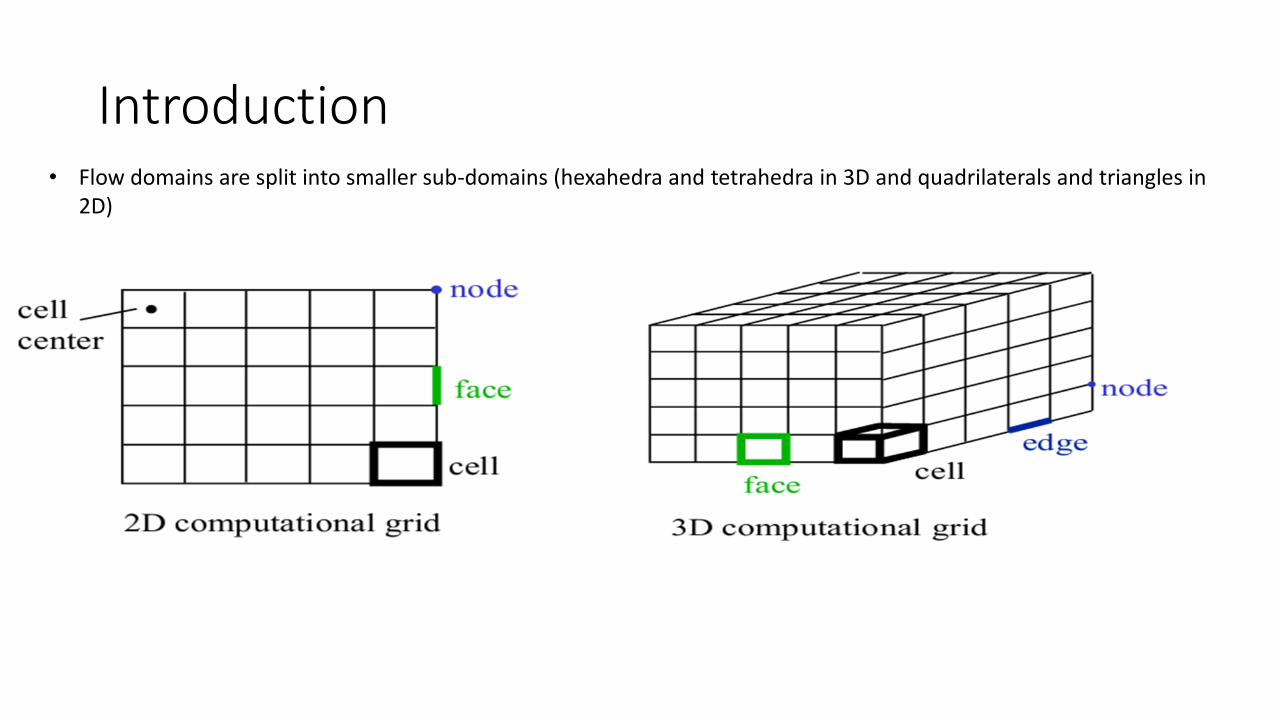
Introduction • Flow domains are split into smaller sub-domains (hexahedra and tetrahedra in 3D and quadrilaterals and triangles in

2D)

Introduction

The grid has a significant impact on

• Rate of convergence

• Solution accuracy

• CPU time required

4

Parameters of mesh quality

Grid density.

Adjacent cell length/volume ratios.(<20%)

Skewness.(<0.85)

Tet vs. hex.

Mesh refinement through adaption.

Orthogonality

Simplest Grid Generation

Finite Difference method Finite Volume method

• Finite Difference Method: Grid points are obtained by the intersection of grid lines (corresponding to the Cartesian or cylindrical or spherical coordinate system)

• Finite Volume Method (Cell centered): Grid points are defined at the centroids of the cells/CVs generated by the intersection of grid lines

Desirable Mesh Properties

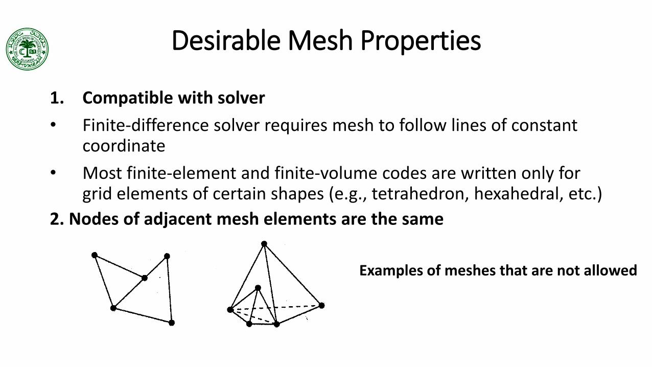
1. Compatible with solver

• Finite-difference solver requires mesh to follow lines of constant coordinate

• Most finite-element and finite-volume codes are written only for grid elements of certain shapes (e.g., tetrahedron, hexahedral, etc.)

2. Nodes of adjacent mesh elements are the same

Examples of meshes that are not allowed

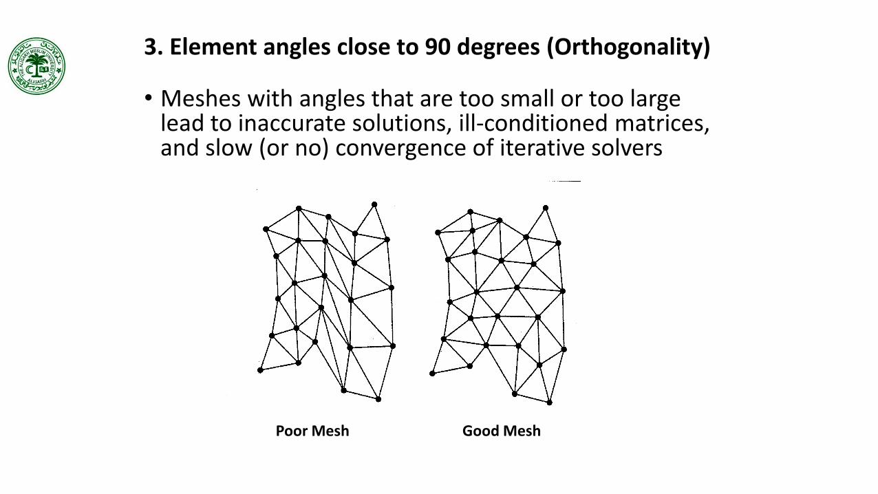
3. Element angles close to 90 degrees (Orthogonality)

• Meshes with angles that are too small or too large lead to inaccurate solutions, ill-conditioned matrices, and slow (or no) convergence of iterative solvers

Poor Mesh Good Mesh

4. Provides adequate resolution of computed fields

• Meshes must be finer in fluid/thermal boundary layers, near cracks in solids, near joints, within vortex cores, etc.

U

5. Uses minimum number of elements

• Triangles use twice as many elements as quadrilaterals

• Tetrahedral use six times as many elements as hexahedral

1

2

3 1

2

6. Easily refinable

• We often want to do tests of resolution by varying the grid size in some systematic manner

• Useful property for multi-grid matrix iteration solvers and multi-scale computational approaches

7. Easy to generate

• Triangles and tetrahedrons are easy to generate using automatic grid generators

• Depends on capabilities of grid generators

8. One to One Correspondence

A mapping which guarantees one-to-one correspondence ensuring grid lines of the same family do not cross each other

Grid Generations Techniques

Structured grids

Algebraic Differential equations

Elliptic

Hyperbolic

Parabolic

Unstructured grids

Grid Generations Techniques

11

STRUCTURED GRID

• Regular connectivity

• Represented by i, j, k indices

• Conserves space

UNSTRUCTURED GRID

• Non-uniform pattern

• Represented by Node numbers

• Large storage requirement

Block Structured Grid

Mesh Generation Concept Structured Grids

Mesh structure: • Domain divided into a structured assembly of quadrilateral cells • Each interior nodal points is surrounded by exactly the same number of mesh cells (or elements) • Directions within the mesh can be immediately identify by associating a curvilinear co-ordinates system • it is possible to immediately identify the nearest neigthbours of any node j on the mesh Advantages: • Large number of algorithms for discretisation are available • The algorithms can be normally implemented in a computationallly efficient manner Disadvantages: • Difficulty to generate grids of regions of general shapes multi-block grids • Very high elapsed time necessary to produce a grid for domains of extremely complex shape

Finite difference, finite volume and finite element discretisations

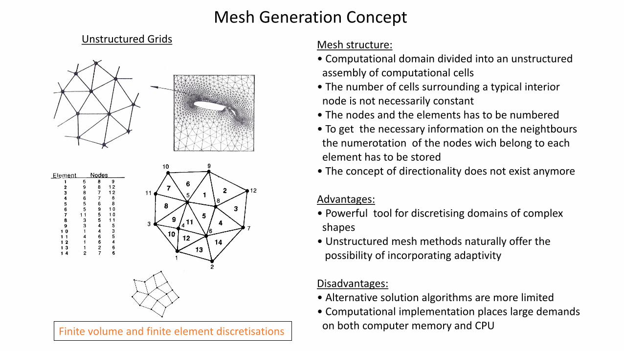
Mesh Generation Concept Unstructured Grids Mesh structure:

• Computational domain divided into an unstructured assembly of computational cells • The number of cells surrounding a typical interior node is not necessarily constant • The nodes and the elements has to be numbered • To get the necessary information on the neightbours the numerotation of the nodes wich belong to each element has to be stored • The concept of directionality does not exist anymore Advantages: • Powerful tool for discretising domains of complex shapes • Unstructured mesh methods naturally offer the possibility of incorporating adaptivity

Disadvantages: • Alternative solution algorithms are more limited • Computational implementation places large demands on both computer memory and CPU Finite volume and finite element discretisations

Geometry Modelling

The boundary of the domain to be discretised needs to be represented in a suitable manner before the generation

can start. If the automatic discretisation of an arbitrary domain is to be achieved, the mathematical description of

the domain topology has to possess the greatest possible generality.

The computer implementation of this description must provide means for automatically computing any geometrical

quantity relevant to the generation procedure.

Planar two-dimensional case

In the planar two dimensional case, the boundary is

represented by closed loops of orientated composite

curves. For simple connected domains these curves

are orientated in a counter-clockwise sense while for

multiple connected regions the exterior boundary curves

are given a counter-clockwise orientation and all the interior

boundary curves are orientated in a clockwise sense

Mathematical description of the geometry → CAD model

Geometry Modelling

Three dimensional case

In three dimensions, the domain to be discretised is viewed as a region bounded by surfaces which intersect

along curves. The portions of these curves and surfaces needed to define the three dimensional domain of

interest are called curve and surface components, respectively.

Decomposition of the boundary of a three dimensional domain into its surfaces and curve components

Geometry Modelling In addition, boundary curves and surfaces are oriented.

This is important in the generating process as it is used

to define the location of the region to be discretised.

The orientation of a boundary surface is defined by the

direction of the inward normal. The orientation of the

boundary curves is defined with respect to the boundary

surfaces that contain them. Each boundary curve will be

common to two boundary surfaces and will have opposite

orientations with respect to each of them.

An example of the approximated geometry of the surfaces

component and its curve components is here

presented.

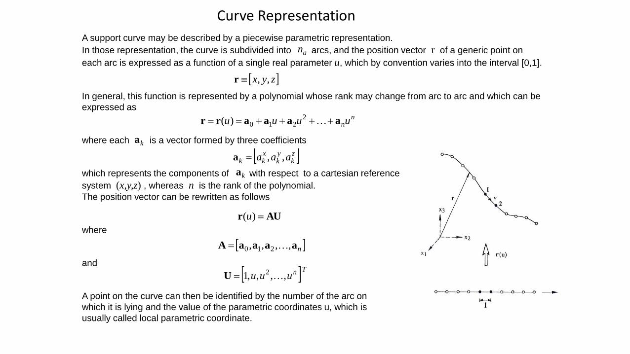
Curve Representation

A support curve may be described by a piecewise parametric representation.

In those representation, the curve is subdivided into arcs, and the position vector r of a generic point on

each arc is expressed as a function of a single real parameter u, which by convention varies into the interval [0,1].

In general, this function is represented by a polynomial whose rank may change from arc to arc and which can be

expressed as

where each is a vector formed by three coefficients

which represents the components of with respect to a cartesian reference

system (x,y,z) , whereas n is the rank of the polynomial.

The position vector can be rewritten as follows

where

and

A point on the curve can then be identified by the number of the arc on

which it is lying and the value of the parametric coordinates u, which is

usually called local parametric coordinate.

an

zyx ,,r

nnuuuu aaaarr 2

210)(

ka

zk

yk

xkk aaa ,,a

ka

AUr )(u

naaaaA ,,,, 210

Tnuuu ,,,,1 2 U

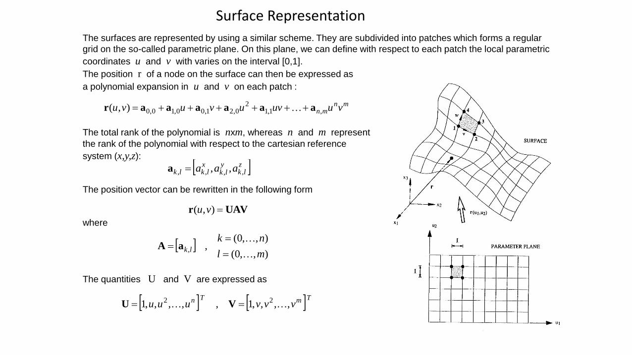
Surface Representation

The surfaces are represented by using a similar scheme. They are subdivided into patches which forms a regular

grid on the so-called parametric plane. On this plane, we can define with respect to each patch the local parametric

coordinates u and v with varies on the interval [0,1].

The position r of a node on the surface can then be expressed as

a polynomial expansion in u and v on each patch :

The total rank of the polynomial is nxm, whereas n and m represent

the rank of the polynomial with respect to the cartesian reference

system (x,y,z):

The position vector can be rewritten in the following form

where

The quantities U and V are expressed as

mnmn vuuvuvuvu ,1,1

20,21,00,10,0),( aaaaaar

zlk

ylk

xlklk aaa ,,,, ,,a

UAVr ),( vu

),,0(

),,0(,

ml

nkk,l

aA

TmTn vvvuuu ,,,,1,,,,,1 22 VU

19

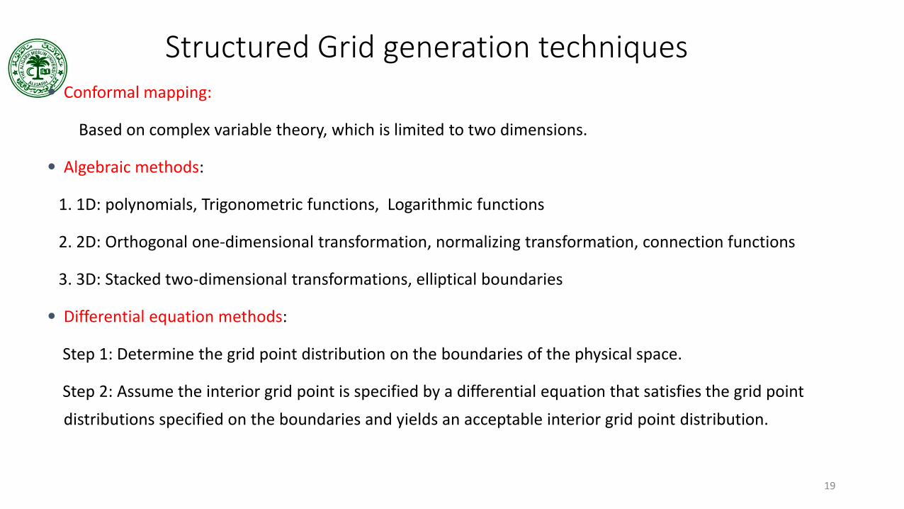
Structured Grid generation techniques • Conformal mapping:

Based on complex variable theory, which is limited to two dimensions.

• Algebraic methods:

1. 1D: polynomials, Trigonometric functions, Logarithmic functions

2. 2D: Orthogonal one-dimensional transformation, normalizing transformation, connection functions

3. 3D: Stacked two-dimensional transformations, elliptical boundaries

• Differential equation methods:

Step 1: Determine the grid point distribution on the boundaries of the physical space.

Step 2: Assume the interior grid point is specified by a differential equation that satisfies the grid point

distributions specified on the boundaries and yields an acceptable interior grid point distribution.

Mappings and Jacobians

Consider the continuous mapping of the form . If a function f exists for which

then

For any differential function f(x) , it is clear that the change of f with respect to is equal to the change of f with

respect to x multiplied by a scaling parameter J which is the change of x with respect to the new variable .

Using this equation to solve for gives

The term is called the jacobian of the mapping and can be seen to be an effective scaling introduced

through the change of variables. The quantity is the ratio of the length in the physical space to the length

in the logical space. If the Jacobian vanishes within the domain, then the transformation is invalid

In two dimensions, let consider a continuous transformation of the form

If we consider a function f with

then

)(xx

)(xff

xJ

x

fJ

x

x

ff,

xf /

f

Jx

f 1

/xJ

/x

),(,),( yyxx

),( yxff

y

y

fx

x

ff

y

y

fx

x

ff

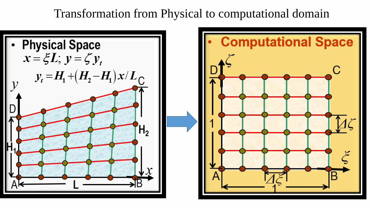
Transformation from Physical to computational domain

• Transformation:

• Inverse Transformation:

Algebraic Grid Generation: Clustering at y=0

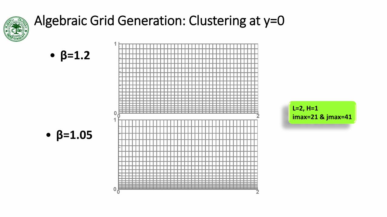
• β=1.2

• β=1.05

Algebraic Grid Generation: Clustering at y=0

L=2, H=1 imax=21 & jmax=41

• Transformation:

• Inverse Transformation:

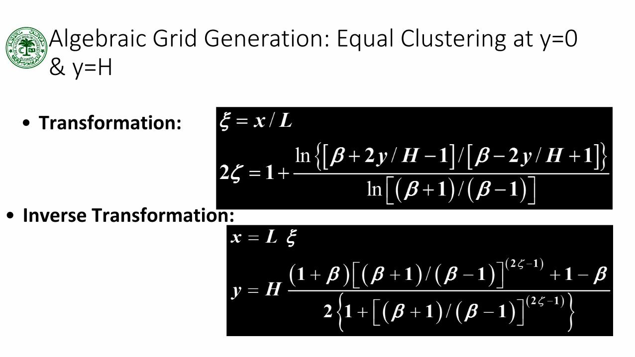
Algebraic Grid Generation: Equal Clustering at y=0 & y=H

• β=1.2

• β=1.05

Algebraic Grid Generation: Equal Clustering at y=0 & y=H

L=2, H=1 imax=21 & jmax=41

• Transformation:

• Inverse Transformation:

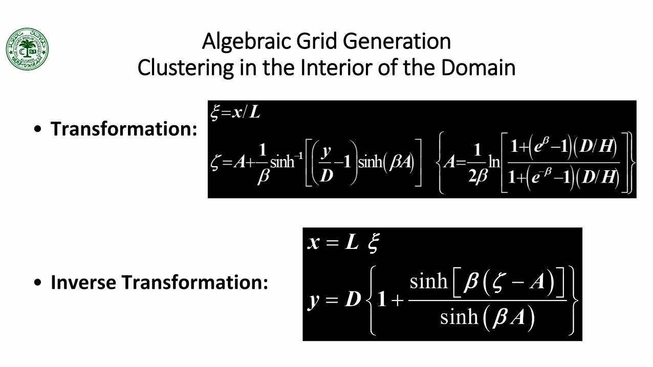
Algebraic Grid Generation Clustering in the Interior of the Domain

• D=H/4 β=5

• D=H/2;β=5 • D=H/2;β=10

Algebraic Grid Generation: Clustering in the interior of the Domain

L=2, H=1 imax=21 & jmax=41

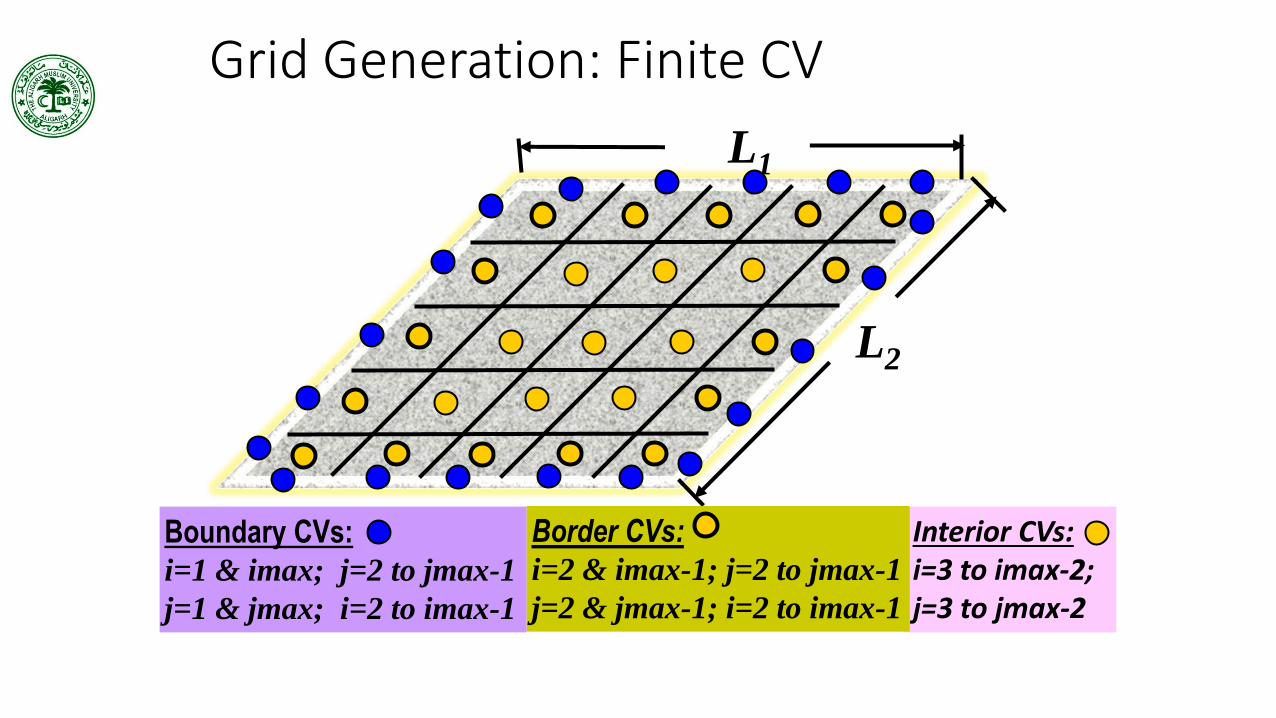
Grid Generation: Finite CV

Boundary CVs:

i=1 & imax; j=2 to jmax-1

j=1 & jmax; i=2 to imax-1

L2

L1

Interior CVs: i=3 to imax-2; j=3 to jmax-2

Border CVs:

i=2 & imax-1; j=2 to jmax-1

j=2 & jmax-1; i=2 to imax-1

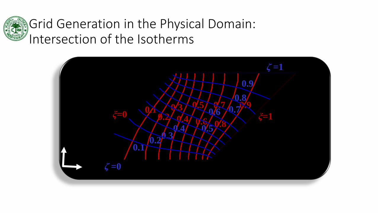
Grid Generation in the Physical Domain: Intersection of the Isotherms

ξ=0 0.1

0.2 0.4

0.9

ξ=1 0.8

0.7 0.3 0.5

0.6

ζ =0

0.1 0.2

0.4

0.9

ζ =1

0.8

0.7

0.3 0.5

0.6

x

y

Elliptic Grid Generation: Inverse Transformation

ξ=0 0.1

0.2 0.4 0.9 ξ=1

0.8 0.7 0.3 0.5

0.6

ζ =0

0.1

0.2

0.4

0.9

ζ =1

0.8

0.7

0.3

0.5

0.6

ξ

ζ

ξ=0 0.1 0.2

0.4

0.9

ξ=1 0.8

0.7 0.3 0.5

0.6

ζ =0

0.1 0.2

0.4

0.9

ζ =1

0.8 0.7

0.3 0.5 0.6

x

y

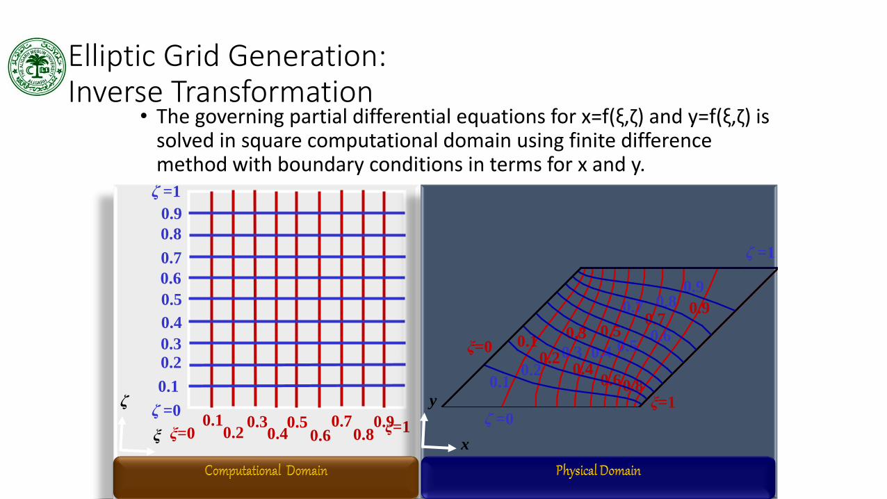
• The governing partial differential equations for x=f(ξ,ζ) and y=f(ξ,ζ) is solved in square computational domain using finite difference method with boundary conditions in terms for x and y.

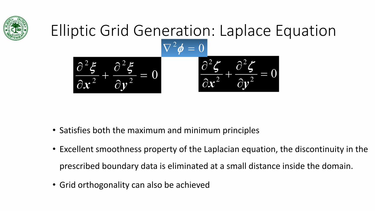
• Satisfies both the maximum and minimum principles

• Excellent smoothness property of the Laplacian equation, the discontinuity in the

prescribed boundary data is eliminated at a small distance inside the domain.

• Grid orthogonality can also be achieved

Elliptic Grid Generation: Laplace Equation

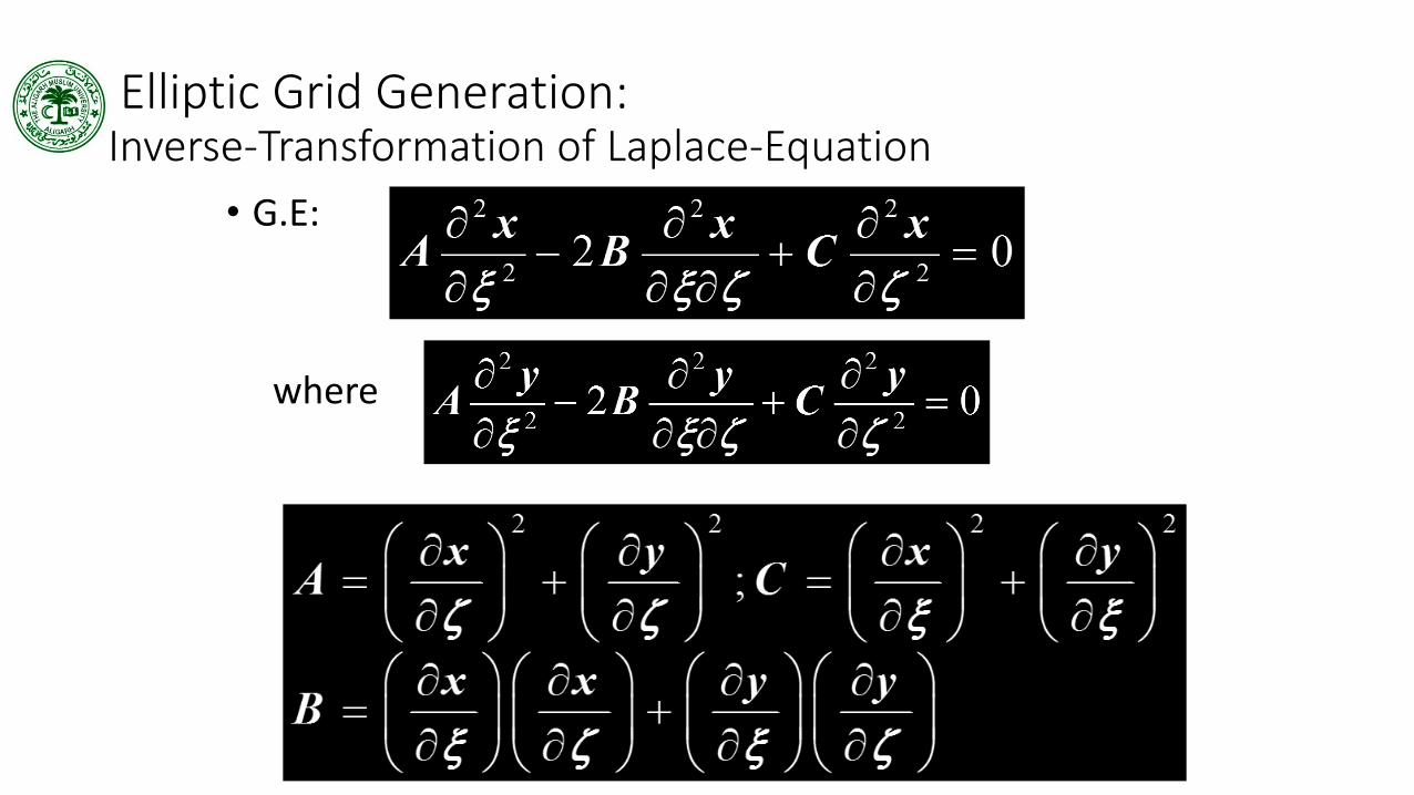
• G.E:

where

Elliptic Grid Generation: Inverse-Transformation of Laplace-Equation

• Condition

• Top/Bottom Boundary: Horizontal Lines

• Left/Right Boundary: Inclined Lines

Grid Orthogonality at the Domain Boundary

PDE’s Grid Generation

• A system of PDEs is solved for the location of grid points in the physical space

• The computational space/domain is a square shaped with uniform grid spacing.

• Types • Elliptic

• Parabolic

• Hyperbolic

Discrete Representation of Domain: Grid Generation

L2

i

j

1 imax 1

jmax Boundary Grid Point: i=1 & imax;

j=2 to jmax-1

j=1 & jmax;

i=2 to imax-1

Border Grid Point: i=2 & imax-1;

j=2 to jmax-1

j=2 & jmax-1;

i=2 to imax-1

i-1,j

i,j+1

i+1,j

i,j-1

i,j

Interior Grid Point:

i=2 to imax-1;

j=2 to jmax-1

L1

i+1,j+1

i+1,j-1

i-1,j+1

i-1,j-1

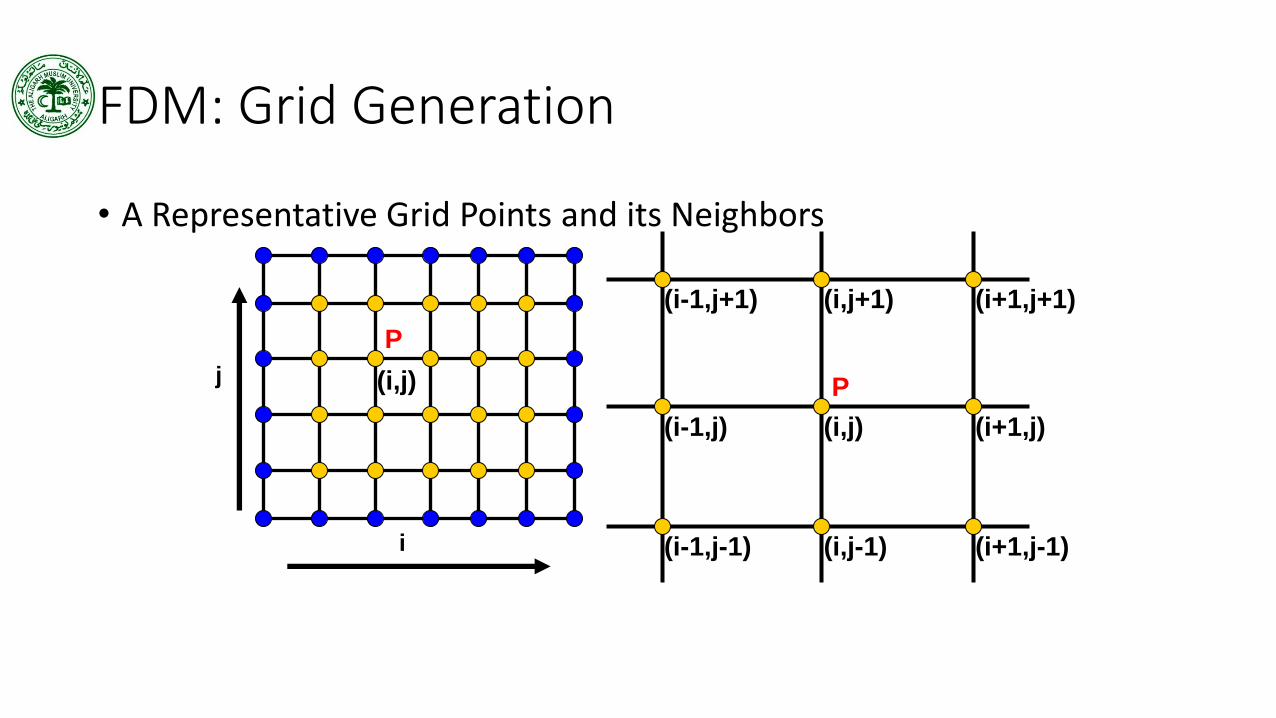
FDM: Grid Generation

• A Representative Grid Points and its Neighbors

(i,j)

P

P

(i,j) (i+1,j) (i-1,j)

(i,j+1) (i+1,j+1) (i-1,j+1)

(i,j-1) (i+1,j-1) (i-1,j-1) i

j

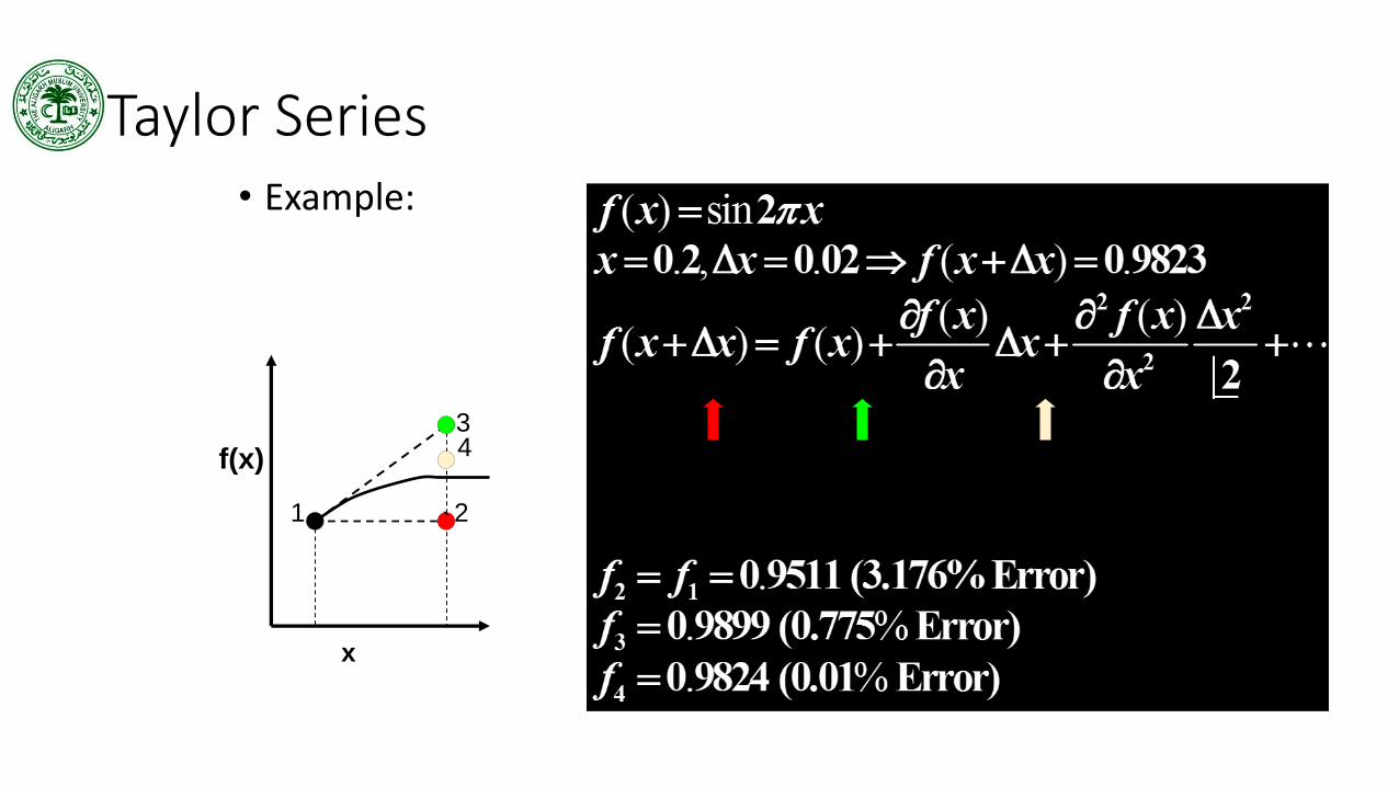
Taylor Series • Example:

I Guess Add to

Capture Slope

Add to account

for Curvature 1 2

3 4

x

f(x)

`

FDM: Taylor Series Expansion

FDM: I Order Forward Difference

Δx

i+1

(+) (-)

i

Finite Difference Quotient

Truncation Error

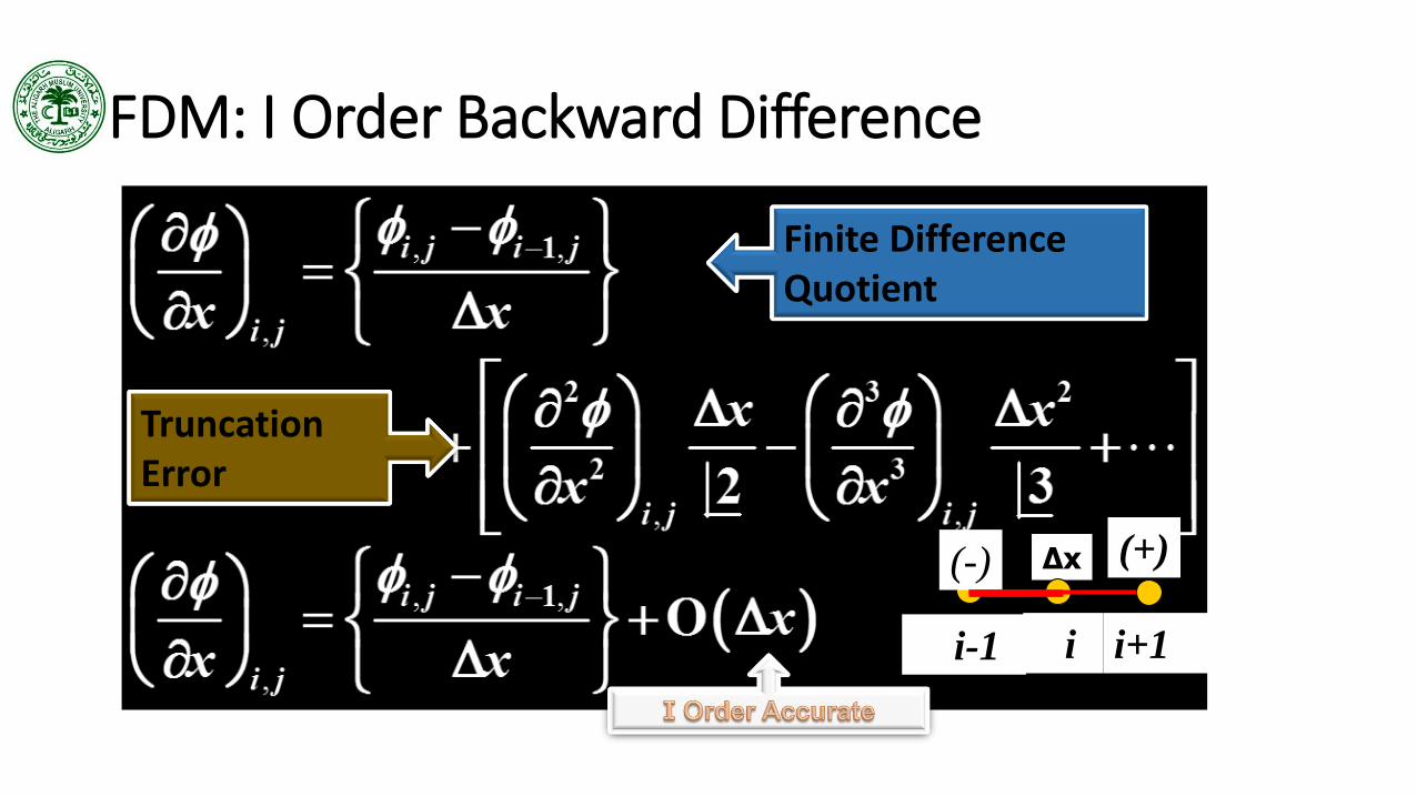
FDM: I Order Backward Difference

Δx

i+1

(+) (-)

i-1 i

Finite Difference Quotient

Truncation Error

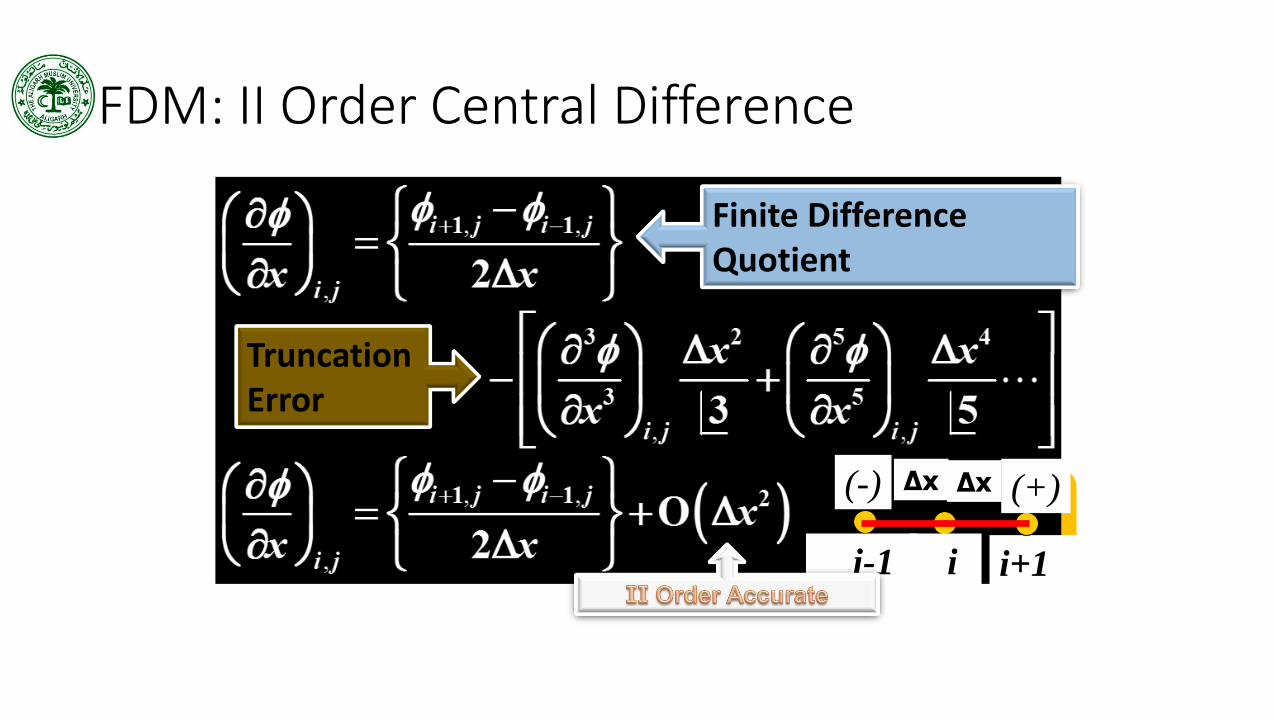
FDM: II Order Central Difference

i+1

(+) (-)

i-1 i

Δx Δx

Finite Difference Quotient

Truncation Error

FDM: II Order Central Second Cross Derivative Difference

i+1,j+1

(+) (-)

Δx Δx

i+1,j-1 i-1,j-1

i-1,j+1

Δy

Δy (+) (-) i,j

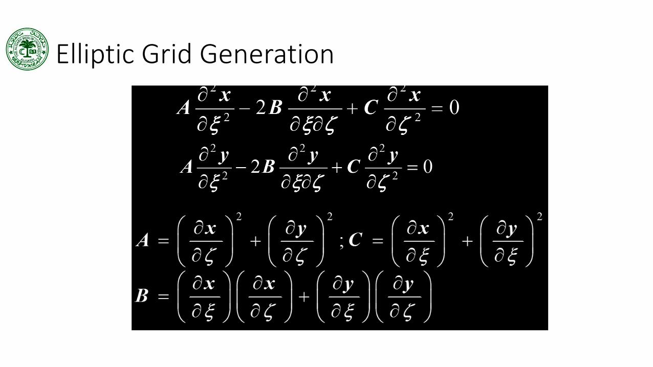
• G.E:

where

Elliptic Grid Generation

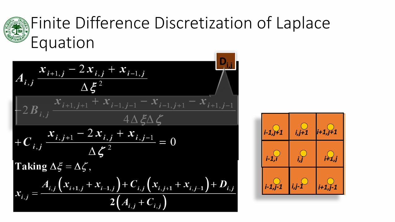
Finite Difference Discretization of Laplace Equation

i,j-1

i-1,i i,j i+1,j

i,j+1

Di,j

i+1,j+1

i+1,j-1 i-1,j-1

i-1,j+1

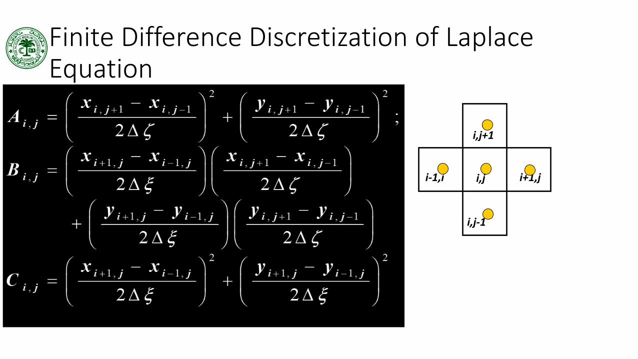
Finite Difference Discretization of Laplace Equation

i,j-1

i-1,i i,j i+1,j

i,j+1

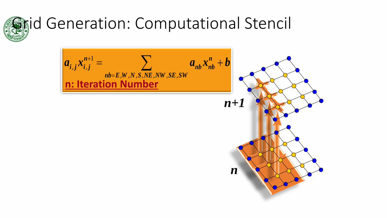
n+1

n

n: Iteration Number

1

, ,

, , , , , , ,

n n

i j i j nb nb

nb E W N S NE NW SE SW

a x a x b

Grid Generation: Computational Stencil

Grid Generation: Solution Algorithm

1. Enter imax, jmax and declare the matrix for x, y, xold and yold

2. Calculate dzi=1/(imax-1) and dzeta=1/(jmax-1)

3. Enter the initial guess for x and y

4. Enter the BC for x and y

5. xold=x and yold=y

6. Using xoldi,j and yoldi,j, For i=2,imax-1 and j=2,jmax-1, Calculate 1. Ai,j, Bi,j, Ci,j, and Di,j

2. xi,j and yi,j

7. Check whether the maximum of abs(xi,j-xoldi,j) and abs(yi,j-yoldi,j) for all interior grid points between two consecutive iteration is less than ε (for ex.: 10-3, practically zero). If not, go to step 5 and continue till convergence

Grids for Multiply connected Domains: Hole in a Square Plate

Grid Generation: O-Type Structured Grids

1

1 ξ

ζ

x

y

Δζ

Δξ

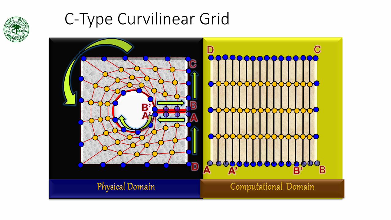
C-Type Curvilinear Grid

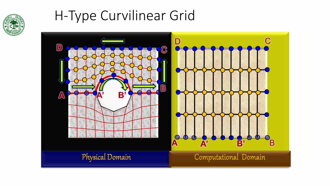
H-Type Curvilinear Grid

Hyperbolic Grid Generation

• Body conforming meshes

• Outer boundary is not specified

• Orthogonal grids

• Faster method

57

Hyperbolic Grid Generation

• Cell Volume scheme- Steger and Chausse

K=40,

• Condition of orthogonality

58

. ( , ) (1)dx dy x y x y V

. 0 (2)x x y y

(1 )

11V K g e 4

2 2

11g x y

11

Vx y

g

11

Vy x

g

Algorithm

Step 1 • Input the body over which grid is to be generated

Step 2 •Calculate and at =0 level(Central difference)

Step 3 •Calculate g11 and V

Step 4 •Calculate and

Step 5

• Integrate in direction by 1 step

• x i,j+1=x i,j +

• y i,j+1=y i,j +

59

x x

x y

.x

.y

Hyperbolic grid over cylinder

• Requirement: Local Fine Grid Clustering near the cylinder

•Does not allow local refinement but creates a horizontal/vertical band of fine grid 4B

4B

1.5B

1.5 B

5 10 15 20 250

5

10

15

20

4B

4B

Grid Generation: Flow across a Cylinder

X

Y

0 10 200

5

10

15

20

3

1

5

24

MultiBlock Structured Grid: Flow across a Circular Cylinder

• Structured Grid: Numerically efficient but less geometrical flexibility of local grid refinement

• Unstructured Grid: Greater geometrical flexibility but less numerically efficient.

• Multi-Block Structured Grid

• The physical domain is divided into regions, called blocks.

• Geometrical flexibility better than structured but worse than unstructured grid.

• They are globally(in-between the blocks) unstructured but locally(within a block) structured

• This block structuring can be viewed as compromise between high geometrical flexibility of fully

unstructured grids and highly numerically efficient structured grids.

• Natural Basis of Parallelization

Types of Grid Generation

Questions and Suggestions