K Ho-Le

An attempt is made to provide o clear overafl picture of the finite element mesh generatlon field. A scheme for c/ossify- ing mesh generation methods is proposed, whereby seven molar mesh generation approaches are identified. The basis for classification is the temporal order in which nodes and elements ore created. The published mesh generation methods ore reviewed. Only four approaches ore found to have fully automatic mesh generation methods. These ap- proaches ore compared on the criteria of element types and shapes, mesh density control, end time efficiency.

computer-aided design, finite element methods, mesh generation

The finite element method is a powerful and versatile analysis tool, but its usefulness is hampered by the need to generate a mesh, but can be very time-consuming and error-prone if done manually. In recognition of this prob- lem, a large number of methods have been devised to auto- mate the mesh generation task. This paper attempts to provide a clear overall picture of the finite element mesh generation field by reviewing, classifying and comparing the mesh generation methods.

There are few comprehensive reviews of mesh generation methods. Buell and Bush z reviewed the pre1973 literature but the field has expanded considerably since then. Thacker 2 published an extensive bibliography in 1980, but did not classify or compare the methods. The material in this paper is more up to date, and appears to be the first attempt at a systematic classification of the methods.

Devising a classification scheme for the mesh generation methods is difficult, and so is the placement of individual methods into the mesh generation classes. Some methods do not seem to fit into any class, while others could be put in two or more places. The final placement is neces- sarily somewhat arbitrary. However it is felt that the clarity afforded by the classification outweighs any prob- lems involved in the classification.

The organization of the paper is as follows. The next section gives some useful background information. The classification scheme is then proposed, followed by the review of 2D and 3D mesh generation methods. Finally, the mesh generation classes are compared on four criteria: element types, element shapes, mesh density control, and time efficiency.

CSIRO Division of Manufacturing Technology, Locked Bag No. 9, Preston 3072, Victoria, Australia

Figure I. Dirichlet tessellation (solid lines) and the Delouney triangulation (dashed lines) on e point set

BACKGROUND INFORMATION Delaunay triangulation Many mesh generators produce a mesh of triangles by first creating all the nodes and then connecting the nodes to form triangles. The question arises as to what is the 'best' triangulation on a given set of points. One particular scheme, namely the Delaunay triangulation, is considered by many researchers 3-s to be the most suitable for finite element analysis. This triangulation maximizes the sum of the smallest angles of the triangles 6 ; thus thin elements are avoided wherever possible.

The Voronoi diagram 4'7-9 of a set of N points in a plane consists of N polygons V(i), each centred on point i such that the locus of points on the plane nearest to node i are included in V(i). The Delaunay triangulation is obtained by connecting the points associated with neighbouring Voronoi polygons (see Figure 1). The above definitions extend naturally to higher-dimensional spaces.

Conversion of element types If a mesh generator produces only one type of element, the elements can be converted to another type as desired. Quad- rilaterals and bricks are easily converted to well-shaped triangles and tetrahedra of similar sizes (see Figure 2). Triangles and tetrahedra may be subdivided into quadri- laterals and bricks (see Figure 3), but the resulting elements are not well-shaped, because the angles around the newly

Finite element mesh generation methods: a review and classification

volume 20 number I jan/feb ] 988 0010-4485/88/010027-12 $03.00 © 1988 Butterworth & Co (Publishers) Ltd 27

d

Figure 2. Conversion o f the quadrilateral into triangles, and the brick into tetrahedra

introduced nodes are necessarily large. Heighway ~° gives a technique to convert a mesh of triangles into a mesh of quadrilaterals by combining every two adjacent triangles into a quadrilateral.

Mesh smoothing

Often the elements produced by an automatic mesh gene- rator are not well-shaped, in which case it is useful to apply a mesh smoothing technique to improve the mesh. The most popular technique is Laplacian smoothing which seeks to reposition the nodes such that each internal node is at the centroid of the polygon formed by its connected neighbours. This repositioning is usually done iteratively, however, a direct solution scheme has also been reported 11 .

In some cases, the Laplacian smoothing technique does not work well; for example, the case illustrated in Figure 4(a). To redress the problem, Herrmann 12 proposes to reposition an internal node i as follows (cf. Figure 5)

1 N Pi - ~ (Pnj + Pn / - wPnk) (1)

N (2-w) n = l

where N is the number of elements around the node i, and w is the weighting factor, 0 ~< w ~< 1.

If w = O, Laplacian smoothing results. If w = 1, the smoothing is called 'isoparametric'; the mesh quality appears to improve (see Figure 4(b)).

Mesh density and mesh conformity

A mesh must accommodate changes in element sizes from region to region. Most FEM packages require a mesh to be conforming, where adjacent elements share a whole edge or a whole face (Figure 6(a)). A mesh composed of triangles or tetrahedra can easily be made conforming, but the task is more difficult with a mesh of quadrilaterals or bricks. Two approaches for creating a transition from large quadri- laterals to small quadrilaterals are illustrated in Figure 7.

Figure 3. Conversion o f the triangle into quadrilaterals, and the tetrahedron into brichs. A new node must be introduced in each case

a b Figure 4. (a) Lap/acian smoothing, and (b) isoparametric smoothing (after Herrmann 12)

When a mesh is refined, some elements are subdivided into smaller elements while others remain unchanged. The question is how to keep the mesh conforming without the introduction of distorted elements. This is difficult with quadrilateral meshes. For triangular meshes, a triangle can be divided into two smaller ones by bisecting the longest side 13. The diagonal transpose technique 4, illustrated in Figure 8, can also be used during the refinement process to create a Delaunay triangulation. However, the elements are not refined in place as required by some adaptive mesh refinement methods, such as the multigrid method 14.

If mesh conformity is allowed to be violated, mesh refinement as well as transitioning between coarse- and fine-mesh regions become easier. In a nonconforming mesh, several small elements may abut a larger one (see Figure 6(b)). Multipoint constraints IsA6 can be applied to the midside nodes to make the mesh analysable. Some novel elements have been introduced to model a large element having many smaller ones abutting its sides 17-19. See also Kela et aL 20 Rheinboldt and Mesztenyi 21 and Simpson 22.

CLASSIFICATION OF MESH GENERATION METHODS In this section, the mesh generation methods, automatic or not, are classified. The methods are still evolving; the ones that are not completely automatic at the moment may become so in the future, so it is worthwhile including them here. For ease of exposition, the proposed classification scheme is explained in terms of 2D mesh generation, but the scheme is applicable to 3D as well.

The output of a mesh generator consists of a set of

ni

Figure 5. Neighbourhood o f an internal node i (after Herrmann 12)

nl

nk'

28 computer-aided design

a b Figure 6. (a) Conforming mesh, and (b) nonconforming mesh, where several small elements may abut a larger one

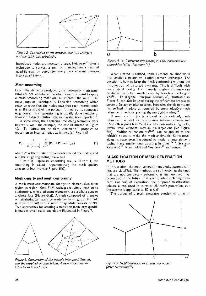
nodes, and a set of elements (which represents the mesh topology). It is proposed to classify the mesh generation methods according to the temporal order of the creation of these sets. There are four main cases as shown in Figure 9.

Mesh topology first The mesh topology is determined first, followed by the nodal positions. Once the mesh topology has been deter- mined, the mesh smoothing techniques described previously may be used to calculate the position of the nodal points. The problem with this approach is that there is no known algorithm for creating the mesh topology, except by using other automatic mesh generation methods! Since mesh smoothing has already been explained, this case will be dropped from further discussions.

Nodes first The nodes are created first, and they are then connected to form triangular or quadrilateral elements. This can be divided into two subcases. If the vertexes of the object are assumed to be the only nodes in the mesh, a triangulation algorithm can be applied to create a minimum number of nonoverlapping triangles that cover the object (see Figure 10). This minimal set of triangles is determined mainly by the topology of the object. The complex topology of the object has been decomposed into the simple topology of the triangles, so this approach will be called the topology decomposition approach. The mesh thus created has dis- torted and mostly coarse elements, and cannot be used for analysis purposes. Mesh refinement, possibly with element rearrangements by the diagonal transpose tech- nique, must be applied to produce a reasonable mesh.

/ \ /

a b Figure 7. Transition from large to small quadrilaterals: (a) with triangles, and (b) with quadrilaterals only

Figure 8. Diagonal transpose to maximize the smallest angle in the triangles

The mesh refinement step above can be avoided if all the nodes in the final mesh are already generated such that their distribution conforms to the mesh density specifi- cation. Then, in the element generation phase, one only has to consider how to connect the nodes to form the best possible elements. This approach (see Figure 11), which covers the bulk of the mesh generation literature, will be called the node connection approach.

Adapted mesh template A mesh template is pregenerated elsewhere, and then adapted to the object being meshed. Three approaches within this case can be identified.

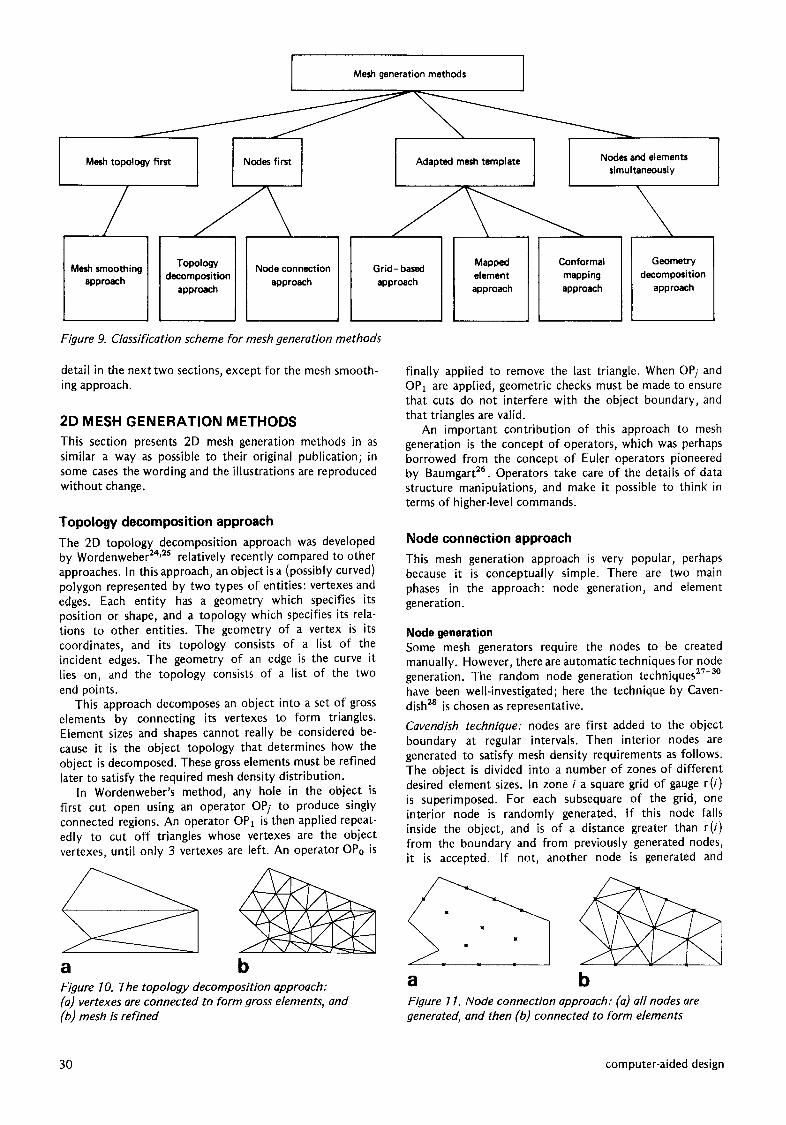
Grid-based approach The mesh template is an infinite rectangular or triangular grid. The grid is superimposed on the object. The grid cells that fall outside the object are removed. The grid cells that intersect the object boundary are adjusted or trimmed so that they fit into the object. The result is a mesh with excellent interior elements (see Figure 12). This approach is becoming popular, especially in 3D mesh generation.

Mapped element approach The mesh template is a rectangular mesh in the unit square (or a triangular mesh in a unit triangle) in the parametric space. It is mapped onto a four-sided (or three-sided) region to induce a mesh in the region via a blending function 23. An arbitrary object has to be subdivided manually into three- or four-sided regions, which are in effect macro elements (see Figure 13). This approach is the mainstay of existing commercial mesh generators.

Conformal mapping approach A polygon Q that has the same number of vertexes as the simply-connected region to be meshed (represented by a polygon P) is constructed such that it can be readily mesh- ed. A conformal mapping F from Q to P is found, based on the correspondence between their vertexes. The mesh in the polygon Q is then mapped onto the object P by this conformal mapping (see Figure 14). This approach is relatively undeveloped compared to other approaches.

Nodes and elements created simultaneously

The nodes and the elements are created simultaneously, with no distinctive phases that can be labeled 'nodes only' or 'elements only'. In this approach, an attempt is made to generate good elements by considering the object geometry, in contrast to the topology decomposition approach which mostly ignores the geometry (except for interference check- ing purposes). This approach will be called the geometry decomposition approach. Figure 15 illustrates a representa- tive method of this approach.

There are altogether seven classes of mesh generation methods as shown in Figure 9, each of which represents an approach to mesh generation. They will be explained in

volume 20 number 1 january/february 1988 29

Mesh topology first

/ Mesh smoothing

approach

Mesh generation methods

Nodes first Adapted mesh template 1 [

Topology decomposition

approach

Node connection approach

G rid- based approach

Mapped element approach

Conformal mapping approach

Nodes and elements simultaneously

Geometry decomposition

approach

Figure 9. Classification scheme for mesh generation methods

detail in the next two sections, except for the mesh smooth- ing approach.

2D MESH GENERATION METHODS This section presents 2D mesh generation methods in as similar a way as possible to their original publication; in some cases the wording and the illustrations are reproduced without change.

Topology decomposition approach The 2D topology decomposition approach was developed by Wordenweber 24p5 relatively recently compared to other approaches, In this approach, an object is a (possibly curved) polygon represented by two types of entities: vertexes and edges. Each entity has a geometry which specifies its position or shape, and a topology which specifies its rela- tions to other entities. The geometry of a vertex is its coordinates, and its topology consists of a list of the incident edges. The geometry of an edge is the curve it lies on, and the topology consists of a list of the two end points.

This approach decomposes an object into a set of gross elements by connecting its vertexes to form triangles. Element sizes and shapes cannot really be considered be- cause it is the object topology that determines how the object is decomposed. These gross elements must be refined later to satisfy the required mesh density distribution.

In Wordenweber's method, any hole in the object is first cut open using an operator OPj to produce singly connected regions. An operator OPz is then applied repeat- edly to cut off triangles whose vertexes are the object vertexes, until only 3 vertexes are left. An operator OPo is

a

finally applied to remove the last triangle. When OPi and OPz are applied, geometric checks must be made to ensure that cuts do not interfere with the object boundary, and that triangles are valid.

An important contribution of this approach to mesh generation is the concept of operators, which was perhaps borrowed from the concept of Euler operators pioneered by Baumgart 26. Operators take care of the details of data structure manipulations, and make it possible to think in terms of higher-level commands.

Figure I0. The topology decomposition approach: (a) vertexes are connected to form gross elements, and (bJ mesh is refined

Node connection approach This mesh generation approach is very popular, perhaps because it is conceptually simple. There are two main phases in the approach: node generation, and element generation.

Node generation Some mesh generators require the nodes to be created manually. However, there are automatic techniques for node generation. The random node generation techniques 2q-3° have been well-investigated; here the technique by Caven- dish 28 is chosen as representative.

Cavend/sh technique: nodes are first added to the object boundary at regular intervals. Then interior nodes are generated to satisfy mesh density requirements as follows. The object is divided into a number of zones of different desired element sizes. In zone i a square grid of gauge r(i) is superimposed. For each subsequare of the grid, one interior node is randomly generated. If this node falls inside the object, and is of a distance greater than r(i) from the boundary and from previously generated nodes, it is accepted. If not, another node is generated and

a b Figure 1 I. Node connection approach." (a) all nodes are generated, and then (b) connected to form elements

30 computer-aided design

y

Z

, I / I I I I i

Figure 1 2. Grid-based approach: interior grid cells give good elements; grid cells along the boundary must be adjusted or trimmed

checked. A fixed number of attempts, say 5, are made to generate an acceptable node for each subsquare, if none is successful then that subsquare is not considered further.

Nonrandom techniques: two such techniques for node generation are known. In Lo's method 31, horizontal lines with spacing I, where / is the desired element length, are intersected with the object. Nodes at approximately dis- tance / apart are placed on the portions of the lines inside the object to produce a uniformly distributed point set. Lee 32 uses the CSG representation for a 2D object that is created by the solid Boolean operations, such as inter- section, union, and difference, on the primitives (e.g. circles and rectangles). In each primitive a node pattern of uniform distribution can be easily generated. These nodes are then combined to produce well-distributed nodes depending on the Boolean operations specified. Some nodes in the overlapping regions may need to be deleted, others may need to be merged or moved.

Element generation In this phase, nodes are connected to form elements such that no elements overlap and the entire object is covered. Most methods produce triangular elements; an excep- tion is Lee's method which attempts to generate quadri- laterals 32 .

In Lee's method, a square grid whose spacing is the same as the desired element size is superimposed on the object. The nodal points are 'bucketed' in the grid cells. The cells are visited in a columnar manner from left to right, and within the same column, from bottom to top. Within a cell, the points are sorted in ascending x-coordinates. Points having the same x-coordinate are sorted in ascending y- coordinates. The points are visited in turn. For each point, neighbouring points are found so as to form the nodes of a good quadrilateral, failing which, a triangle is formed.

Most of the references on node generation above also give triangulation methods. Some other methods are given below.

Lewis and Robinson's method33: this recursive algorithm

a

b

/ / / 1 1

/ /

C Figure 13. Mapped element approach: (a) object is divided into macro elements, and (b) mesh template in unit square is mapped into each element to produce (c) the final mesh

first divides the object into two halves and then keeps on dividing the halves until only triangles remain. An attempt is made to find the split line that best divides the region into two 'equally sized halves' while keeping the halves as 'circular' as possible. For example, for elliptical shapes a split along the minor axis is preferable. Any interior nodes

Q P

Figure 14. Conformal mapping approach: polygon Q and its mesh is constructed in the parametric space, and then mapped onto the object P by a conformal mapping (after Brown s6)

volume 20 number 1 january/february 1988 31

\ Figure 15. Geometry decomposition approach: one element after another is removed from the object

which lie close to the proposed split line are included as part of the new boundaries, thus giving a zigzag effect.

Frederick's method34: each node is to be surrounded with triangular elements. The method begins by selecting a node i, and a node j nearest to i. The side ij is then used to find a node # such that the angle ikj is a maximum and ijk is in a counterclockwise sequence. The new point k then becomes j, and the process is repeated until the node i is fully surrounded with triangles. A new i node is selected and the process is repeated.

Delaunay triangulation methods: these are perhaps the most important triangulation methods because, as men- tioned previously, a Delaunay triangulation maximizes the sum of the smallest angles in all of the triangles in the mesh, thus creating the best mesh for a given set of points. Most of the references on the Delaunay triangulation given pre- viously also contain algorithms for triangulation. Here, another algorithm, by Nelson as , is given.

Nelson's algorithm: start with any boundary segment as a baseline. Find a node which can be connected to Form a triangular element without the resulting element crossing any region boundary, and such that all other nodes fall outside the circle circumscribing the element. Of the two new baselines created by this connection, stack one baseline and let the other be the new current baseline. Whenever the current baseline is a boundary-segment or already occurs in two existing elements, unstack a saved baseline. When the stack is empty, the routine is finished.

Instead of finding the Delaunay triangulation, the method of McGirr et al. ~6 starts by finding the Voronoi diagram. The point associated with each Voronoi polygon can then be connected to the polygon vertexes to form triangles. Many of the resulting triangles, however, appear to be too thin, and have to be searched for and removed.

Grid-based approach The grid-based approach arises out of the observation that a grid looks like a mesh, and it can be made into a mesh provided that the grid cells along the object boundary can be turned into elements. The finer the grid, the better the mesh, since the internal elements which are all well-shaped will become more numerous. The actual methods for mesh construction differ greatly, but the outputs are always similar, since the internal elements are all the same; the only difference being the boundary elements.

The method by Thacker, Gonzalez and Putland a7 is probably the first published one using the grid-based ap- proach. An object is first enclosed in an equilateral triangle fitted with a triangular grid. The grid points that fall out- side the object are eliminated, leaving a zigzag boundary. The grid points on the zigzag boundary are then moved onto the object boundary to create the finished mesh. Kikuchi ~s extends this method to create meshes of pre- dominantly quadrilaterals, but with some triangles, by

using a rectangular grid. One problem with both these methods is that small features, having edges too short compared to the grid spacings, are lost.

Heighway and Biddlecombe 39 start with a zigzag bound- ary that lies entirely within the object, and then mesh the thin strip left between the zigzag boundary and the actual boundary with a triangulation algorithm. The interior elements are initially rectangles but now must be diagonal- ized into triangles.

Kela, Perucchio and Voelcker 2° similarly mesh the interior first with rectangles, but attempt to mesh the boundary strip with quadrilaterals where possible, and triangles otherwise. Only uniform meshes can be generated initially; they may be refined afterwards. They use a CSG representation of the object.

TIPS-1 40, a geometric modelling system, stores a coarse grid as a secondary geometric representation, in addition to the CSG model. This grid could be turned into a mesh by moving the grid points near the boundary onto the boundary; however in the implementation by Akiyama and Wang 41 , this movement has to be done manually.

Yerry and Shephard 42 start with a quadtree encoding of an object 43. This quadtree is modified to be more suit- able to mesh generation as follows:

• The object interior is subdivided into quadrants whose sizes satisfy the mesh density distribution.

• Neighbouring quadrants may differ by at most one level of subdivision.

• The quadrants on the boundary may have cut corners.

Each quadrant is next broken up into triangles such that the resulting mesh is conforming. The triangles, especially the boundary ones, may not be well-shaped.

Mapped element approach This approach requires an object be subdivided manually into simple regions, each of which consists of three or four sides. As such, it is not completely automatic and could have been ignored, were it not for the fact that almost all commercial mesh generators rely on it. Yeung and Hsu 44 made an attempt to automate the division of the object into gross quadrilaterals, but their algorithm is not robust enough. Indeed, if the algorithm had been robust, it could have been extended to generate elements of the right sizes in the first place!

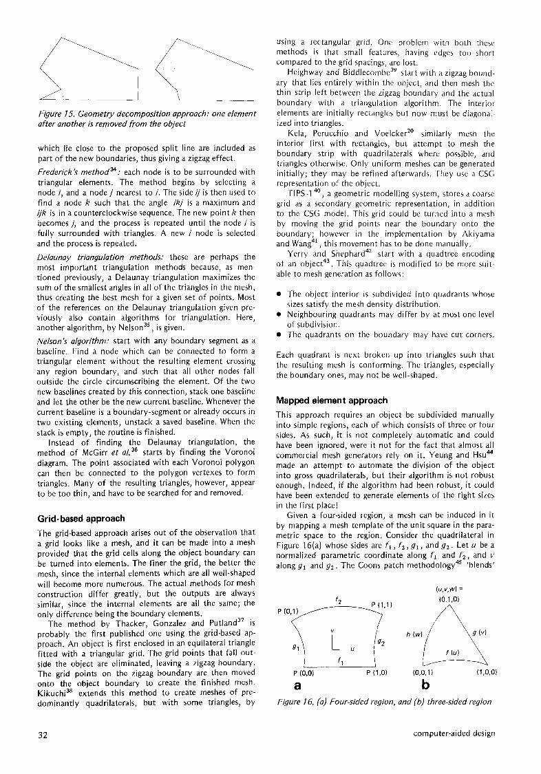
Given a four-sided region, a mesh can be induced in it by mapping a mesh template of the unit square in the para- metric space to the region. Consider the quadrilateral in Figure 16(a) whose sides are f l , f2, g l , and g=. Let u be a normalized parametric coordinate along f l and f 2 , and v along gl and g2. The Coons patch methodology 4s 'blends'

(u,v,w) =

f2 P (1,1) (0,1,0) P

fl

P (0,01 P (1,0) (0,0,11 (1,0,0)

a b Figure 16. (a) Four-sided region, and (b) three-sided region

32 computer-aided design

these sides to give the Cartesian coordinates of a point P(u,v) in the quadrilateral corresponding to a point (u,v) in the unit square in the parametric space. In its simplest form

P(u, v) = (I - v) f l (u) + vf2 (u) + (I - u) gl (v) + ug2 (v)

- (I - u ) ( 1 - v ) P(0,0) - ( I - u ) v P ( 0 , 1 )

- uvP(1,1) - u (I -v) P(I,0) (2)

0 ~ u ~ 1 , 0 ~ v ~ 1

The mesh template in the parametric space can be a rec- tangular grid occupying the unit square; the number of subdivisions in the grid depends on the mesh density dis- tribution. The mesh can also be graded by using unequal u- or v-spacings for the grid lines.

The above blending technique can be formulated in terms of the elegant projector theory ~ , and is called the transfinite mapping technique 47-49. The projector concept allows the generalization of the technique to the use of higher order interpolants to force the coordinate curves to pass through specified curves on the interior of the region s° .

A three-sided region can be similarly divided into a mesh of triangular elements by the use of a trilinearly blended interpolant as described by Barnhill et al. sl. Referring to Figure 16(b), the simplest formulation of the technique is

wh(1 - , ,h(w) 1 ug(v) + + - - P(u,v,w) = ~ [ 1 -v I - v I - w

+ uf(1 -W) + wf(u) + __vg(] -U) _wf(O) 1 - w 1 - u 1 - u

- ug(0) - vh(0) ] (3)

U + V + W = I

O~<u~<l, O~<v~<l, O~<w~<l

The isoparametric mapping is a special case of the trans-

u- plane

w = F (u) z = G (u)

w-plane 9 w= F (G-1IzI)

0} z - plane

Figure I Z Conformal mapping from the polygon Q to the polygon P (after Brown s6)

finite mapping where the boundary curves of a quadrilateral are described by Lagrange polynomials. The technique, first described by Zienkiewicz and Phillips s2, is widely used for mesh generation. In their formulation, two opposite sides of the quadrilateral must have the same number of sub- divisions. In this case, the bandwidth of the object stiffness matrix can be minimized by an appropriate node number- ing scheme. Cohen sa presents a method that allows oppo- site sides to have different numbers of subdivisions.

The discrete transfinite mapping 47 is another special case of the transfinite mapping where a boundary curve is represented as a finite list of points located on the curve, with a unique coordinate associated with each point in the list. The coordinate of the i th point in a boundary curve of n points can be taken as ( i - 1) / (n- I). The boundary curves can be very general. For example, several simpler curves can be concatenated to form a single complex curve. Boundaries that have no exact mathematical description are easily handled.

Yildir and Wexler s4 models the boundaries of a simple region with splines. By using cubic splines or higher order splines, the curvature from one region to another can be made continuous.

C o n f o r m a l m a p p i n g approach

While this approach can deal with simply-connected regions having more than four sides, and hence is more general than the mapped element approach, it is not popular because element shape and mesh density are difficult to control. Three methods based on this approach are known ss-s~. The method by Brown s6 will be described here, as being representative of this approach. This method consists of four steps:

• Step I: model the 2D simply-connected region to be meshed with a straight-sided polygon P in the complex w-plane.

• Step 2: define a polygon Q in the complexz-plane such that Q has the same number of vertexes as P, and a mesh for Q composed entirely of ideally-shaped elements may be generated easily. The mesh topology for Q will be the mesh topology for P.

• Step 3: find the Schwarz-Christoffel transformation G that maps from the upper half u-plane onto the interior of Q, and the transformation F from the upper half u- plane onto the interior of P (see Figure 17).

• Step 4: map the mesh from Q onto P using the compo- site mapping

w = F(G-' (z)) (4)

One problem with this method is that the inverse mapping G -I cannot always be found.

G e o m e t r y d e c o m p o s i t i o n approach

This approach gives some consideration to element shapes and sizes while decomposing an object. Some methods are based on recursion, others on iteration. Representative methods are described below.

In Bykat's method sa, the original object has to be divided into convex parts first. This can be done auto- matically sg. Nodes are next inserted into the boundary of a convex object to satisfy the mesh density distribution. Then the object is divided roughly in the middle of its

volume 20 number I january/february 1988 33

B A

, X

Figure 18. Tracy's algori thm: angles less than 90 ° are cut o f f to form one triangl% and angles between 90 ° and 180 ° are cut o f f to form two triangles

'longest axis'. More nodes are inserted into this split line according to the mesh density distribution. The two halves are recursively divided until they become triangles.

Triquamesh 6°, a commercial mesh generator, is based on a recursive algorithm similar to the above, but uses a different criterion for choosing the split line. It is capable of generating an all-quadrilateral or all-triangle mesh.

An iterative algorithm that removes one or two triangles at a time from the boundary inwards is given by Tracy 61. It assumes the boundary of a singly-connected region has been subdivided into straight line segments whose lengths correspond to the desired element sizes. The algorithm has four steps:

• Step 1: assemble the vertexes of the region in an array, in the counterclockwise order, to form a polygon.

• Step 2: remove all vertex angles of the polygon which are less than 90 ° by forming triangular elements (Fig- ure 18).

• Step 3: start at some vertex B with an angle of less than 180 ° and form two triangles with the adjacent points to the vertex, A and C, and a new point D (see Figure 18). For (XD, YD) use

XA + Xc YA - Yc X D - + - -

2 5

YA + Yc XC-XA Y D - - - + (5)

2 5

where the factor 5 is arbitrary. Update the polygon array by replacing B with D.

• Step 4: check if step 3 creates new angles of less than 90 °. If so, repeat step 2 until it is possible to do step 3 again or the region has only three points left. From the last three points form a triangular element, and the process is complete.

Bykat s9 and Sadek °2 also report similar iterative algorithms. Lindholm's iterative algorithm 63 is slightly different: boun- dary layers, rather than elements, are removed from the object one at a time and then triangulated (see Figure 19).

Figure 19. Lindholm's algorithm: boundary layer is removed from object and triangulated

3D MESH GENERATION METHODS There are very few published 3D mesh generation methods compared to 2D methods due to the greatly increased complexity. While several mesh generation approaches offer the quadrilateral element as an output in 2D, none has been extended to offer the brick element for the 3D case. The following description of the 3D methods is brief because they are based on the same ideas as the 2D methods.

The author is not aware of any 3D mesh generation method based on the conformal mapping approach. The mapped element approach is simple to extend to 3D, so that a mesh can be generated in a four-, five- or six-faced region s2'64,6s . However, as in the 2D case, this approach is not completely automatic, and will not be discussed further. The other four approaches have been extended to 3D, and are reviewed below.

Topology decomposition approach Wordenweber's 2D mesh generation method 24 has been extended to 3D 24'2s. Another method based on the topo- logy decomposition approach, by Woo and Thomasma ~ , is intended solely for 3D, and is given here.

A polyhedral object having holes is first reduced to an object without holes by cutting open the holes with an operator T3 as shown in Figure 20. Three tetrahedra are produced as by-products. An object having no hole is decomposed into tetrahedra by two operators. The opera- tor T1 operates on a convex trivalent vertex (that is, a vertex having three edges) to construct a tetrahedron by cutting out the corner. The operator T2 digs out a tetra- hedron from a convex edge. In either case the tetrahedron must not interfere with any part of the object. Interference is defined by the following two rules:

VT : No vertex of the object lies on any of the four faces of the tetrahedron.

ET : No edge of the object intersects any of the four faces of the tetrahedron.

The algorithm proceeds as follows. If there exists a convex trivalent vertex in the object, then apply the operator TI to construct a tetrahedron T. If T passes interference tests VT and ET, then remove it from the object. Continue with the operator TI on the remaining object. If all the remain- ing vertexes are not convex trivalent, or if all the construct- ed tetrahedra fail the interference tests, then apply the operator T2 to dig out a tetrahedron. If this tetrahedron passes the interference tests, go back to the operator TI . Continue this process until the object is reduced to a single tetrahed ran.

Node connection approach The two following mesh generation methods, based on the node connection approach, require the user to create the nodes manually. The author is not aware of any published algorithm for the automatic generation of nodes in 3D.

Nguyen-Van-Phai 6~ extends Frederick's 2D method to 3D by fully surrounding a line connecting two nearest nodes with tetrahedra. Cavendish 3 uses a 3D Delaunay triangulation algorithm to create tetrahedra. These tetra- hedra form a convex set, with many of them falling outside the object, so each one has to be tested to see if it is inside or outside. The ones outside the object are discarded. It is surprising that while the 2D Delaunay triangulation is, in

34 computer-aided design

i iii.i : a ' .:/

. ; . . il" " i . . '~

o S

b C

Figure 20. Woo and Thomasma's method: (a) operator Tl ." cutting a convex corner, (b) operator T2 : digging out a tetra- hedron, and (c) operator Ta : cutting open a hole (after Woo and Thomasma as)

some sense, the optimal triangulation on a given point set, the 3D Delaunay triangulation may contain very thin tetra- hedra, which must be identified and removed.

Grid-based approach

Of all the six grid-based methods for 2D mesh generation discussed previously, only the one by Yerry and Shephard 6s has been extended to 3D. The object is octree~ncoded 4a, again with some modifications. The octants are broken up into tetrahedra by using a complicated algorithm.

Geometry decomposition approach

Triquamesh 69 appears to be the only 3D mesh generator based on this approach. It recursively divides an object into two subvolumes, by choosing a 'best splitting plane', until all subvolumes have been reduced to tetrahedra. Bricks cannot be generated directly, in contrast to the 2D case where quadrilaterals can be produced by the method. Each tetrahedron may be subdivided into four bricks if desired.

• Step 1 : if the elements generated are not of the desired type, then subdivide them into elements of the desired type.

• Step 2: if the elements do not have sizes compatible with the desired mesh density distribution, then refine them.

• Step 3: if the elements are not well-shaped, then apply a mesh smoothing technique.

The methods for performing these steps have already been discussed. If the postprocessing steps work perfectly, then any initial mesh will do. However, they do not, and the quality of the final mesh depends strongly on the quality of the initial one. Thus the approaches will be compared based on their unprocessed output mesh. Four criteria for comparison are used:

• element type • element shape • mesh density control • time efficiency

COMPARISON OF APPROACHES Comparing the mesh generation approaches is difficult because access to the actual mesh generators is not avail- able. Therefore, it is necessary to make do with the litera- ture and try to infer the capabilities of the approaches.

Only fully automatic mesh generation approaches are compared. This restriction eliminates the two semi- automatic approaches, namely the conformal mapping approach and the mapped element approach. The current implementations of the node connection approach for 3D are not really automatic because nodes must be created manually, but this problem can be easily solved. One possible solution is to superimpose a rectangular grid on the object and choose the grid points that fall inside the object. Therefore this approach should be admitted as an automatic one. Altogether, there are four approaches to be compared: the topology decomposition approach, the node connection approach, the grid-based approach, and the geometry decomposition approach.

Some mesh generation methods, notably the ones based on the topology decomposition approach, do not generate an initial mesh that is good enough for analysis. They rely on postprocessing to improve the mesh. Three postprocess- ing steps can be used:

The criterion of space efficiency is relatively unimportant and hence will not be discussed. Bandwidth or frontwidth optimization, while very desirable, unfortunately cannot be achieved by any automatic mesh generation approaches (but can be done in the semi-automatic approachesS2'ST). Postprocessing must be done to optimize the bandwidth or the frontwidth, using algorithms such as those in Cuthill and McKee 7° and Pina 71.

The mesh generation approaches are now compared. The results of the best implementations of the approaches on each criterion are summarized in Table 1.

Table 1. Comparison of the mesh generation approaches

Approach Quadri- Brick Element Mesh Time lateral shape density efficiency

control

Topological No No Poor No O(N 2 ) decomposition

Node connection Yes No 2D good, Yes O(N) 3D fair

Grid-based Yes Relatively Interior Yes O(N) easy elements

excellent

Geometric Yes No 2D good, Yes unknown decomposition 3D unknown

(N = number of nodes in the mesh)

volume 20 number I january/february 1988 35

Element type The triangle and the tetrahedron are relatively easy to generate, and all approaches can produce them as the primary output. We are interested in the approaches that can also produce the quadrilateral and the brick directly.

In 2D, most methods produce triangles; the exceptions being Lee's method 32 (of the node connection approach), the method of Kela et al. 2° (of the grid-based approach), and Triquamesh 6° (of the geometry decomposition ap- proach). The former two methods produce a mixture of triangles and quadrilaterals; the latter, all quadrilaterals. In 3D, no existing method can produce bricks. The grid- based approach, however, already offers bricks in the object interior, and should therefore be easier than other ap- proaches to coax into generating bricks.

Element shape In the topology decomposition approach, element shapes are determined by the object topology and hence cannot be easily controlled. With careful implementation, all other approaches appear to be capable of generating well-shaped 2D elements; see for example the methods of Lee 32, Kela et al. 2° and Bykat sg. In 3D, the Delaunay triangulation 3 of the node connection approach cannot guarantee well- shaped elements as it does in 2D. The grid-based approach °a gives excellent interior elements and the mesh should be fine overall, though in Yerry and Shephard's implementa- tion, some boundary-elements appear to have poor shapes. The geometry decomposition approach in 3D, as repre- sented by Triquamcsh, cannot be assessed, because details of the method are not available.

Mesh density control The topology decomposition approach cannot control mesh densities directly and has to rely on mesh refinement. The other approaches are all capable of mesh density control, as exemplified by Cavendish et aL 3, Yerry and Shephard 42 and Bykat ss.

Time efficiency Let N be the number of nodes in the output mesh. Worden- weber's method (of the topology decomposition approach) requires O(N 2) time 24. The 2D Delaunay triangulation algorithm by Green and Sibson 9 (of the node connection approach) requires O(N a/2) time, though one can do better by using the linear expected time algorithm of Bentley et a/. ~ as cited in Devroye 73. By using a bucket algorithm, Lee's method (also of the node connection approach) requires only O(N) time. The 3D Delaunay triangulation algorithm by Cavendish 3 requires O(N 2) time. The grid- based approach should require only O(N) by virtue of the spatial addressing property of the grid. The efficiency of the geometry decomposition approach has not been anal- ysed by any author, though Bykat's recursive algorithm in 2D sa has an observed O(N) running time.

CONCLUDING REMARKS In this paper, the published mesh generation methods are reviewed, classified and compared. Seven mesh generation approaches are identified, but only four of them are found to be automatic. The classification scheme presented here is new and may need further refinements. However, it is already useful, not only in showing a clear overall picture of the mesh generation field, but also in giving insights into

the relationship between the approaches. For example, the topology decomposition approach and the node connection approach, two subbranches from a common branch (see Figure 9), both involve a phase where nodal connectivity' is generated from a given point set. Many techniques in the node connection approach, e.g. the Delaunay triangula- tion, would also be applicable to the topology decomposi- tion approach, as far as this phase is concerned.

Accurate comparison of the approaches is difficult, since access to the actual mesh generators is not available. Another reason is that the approaches are still evolving; present limitations in their capability may be overcome later. However, the comparison does give some idea of their potential for 3D mesh generation.

ACKNOWLEDGEMENTS The author wishes to thank Mr R J Maxwell, Dr T F Berreen, Dr T H Siauw, Dr W R Thorpe and Dr M C Good for discussions and helpful comments. This work arises out of a collaborative project between CSIRO and Monash University. The support of CSIRO for this work is greatly appreciated. The author also wishes to thank the referees for suggestions to improve the paper.

REFERENCES I Buell, W R and Bush, B A 'Mesh generation - a survey'

Trans. ASME, J. Eng. Ind. (February 1973) pp 332-338

2 Thacker, W C 'A brief review of techniques for generat- ing irregular computational grids' Int. J. A/umer. Meth. Eng. Vo115 (1980) pp 1335-1341

3 Cavendish, J C, Field, D A and Frey, W H 'An approach to automatic three-dimensional finite element mesh generation' Int. J. Numer. Meth. Eng. Vol 21 (1985) pp 329-347

4 Cendes, Z J, Shenton, D and Shahnasser, H 'Magnetic field computation using Delaunay triangulation and complementary finite element methods' IEEE Trans. Mag. Vol MAG-19 No 6 (November 1983)

5 Boubez, T I, Funnell, W R J, Lowther, D A, Pinchuk, A R and Silvester, P P 'Mesh generation for computa- tional analysis' Comput.-Aided Eng. J. (October 1986) pp 190-201

6 Lawson, C L 'Software for C1 surface interpolation' in Rice, J (ed) Mathematical Software I I I New York Academic (1977)Math. Software Symp. Madison, USA pp 161--193

7 Brostow, W and Dussault, J P 'Construction of Voronoi polyhedra' J. of Computational Physics Vol 29 (1978) pp 81-92

8 Shamos, M I 'Geometric complexity' Proc. 7th Annual A CM 51GA CT Cone (May 1975) pp 224-233

9 Green, P J and Sibson, R 'Computing dirichlet tessella- tions in the plane' The Computer J. Vol 21 No 2 (1977) pp 168-173

10 Heighway, E A 'A mesh generator for automatically subdividing irregular polygons into quadrilaterals' IEEE Trans. on Mag. Vol MAG-19 No 6 (November 1983) pp 2535-2538

11 Denayer, A 'Automatic generation of finite element meshes' Comput. &Struc. Vol 9 (1978) pp 359-364

36 computer-aided design

12 Herrmann, L R 'Laplacian-isoparametric grid genera- tion scheme' J. of Eng. Mech. Div. Proceedings of Amer. Soc. Civil Eng. Vo1102 (EM5) (October 1976)

13 Rivara, M C 'Algorithms for refining triangular grids suitable for adaptive and multi-grid techniques' Int. J. Numer. Meth. Eng. Vol 20 (1984) pp 745-756

14 Brandt, A 'Multi-level adaptive solutions to boundary- value problems' Math. of Computation Vol 31 No 138 (April 1977) pp 333-390

15 Abaqus user's manual Hibbitt, Karlsson, and Sorensen, Inc. (May 1984) Version 4.5

16 Supertab user's manual Structural Dynamics Research Corporation (1986)

17 Gupta, A K 'A finite element for transition from a fine to a coarse grid' Int. J. Numer. Meth. Eng. Vol 12 (1978) pp 35-45

18 Gregory, J A, Fishelov, D, Schut, B and Whiteman, I R 'Local mesh refinement with finite elements for elliptic problems' J. Comput. Physics Vol 29 (1978) pp 133-140

19 Cavendish, J C, Gordon, W ] and Hall, C A 'Substruc- tured macro elements based on locally blended inter- polation' Int. J. Numer. Meth. Eng. Vol 11 (1977) pp 1405-1421

20 Kela, A, Perucchio, R and Voelcker, H B 'Toward automatic finite element analysis' Comput. Mech. Eng. Vol 5 No 1 (July 1986)

Rheinboldt, W C and Mesztenyi, C K 'On a data struc- ture for adaptive finite element mesh refinements' ACM Trans. on Math. Software Vol 6 No 2 (June 1980) pp 166-187

Simpson, R B 'Automatic local refinement for irregular rectangular meshes' Int. J. Numer. Meth. Eng. Vol 14 (1979) pp 1665-1678

Gordon, W J 'Blending-function methods of bivariate and multivariate interpolation and approximation' SIAM J. Numer. Anal. Vol 8 No 1 (1971) pp 158-177

24 Wordenweber, B 'Volume triangulation' Technical Report University of Cambridge, UK, CAD Group Document No. I I0 (1980)

25 Wordenweber, B 'Finite element mesh generation' Comput.-Aided Des. Vol 16 No 5 (September 1984) pp 285-291

26 Baumgart, B G 'Geometric modeling for computer vision' Report No. C5-463 Stanford Artificial Intelli- gence Laboratory, Computer Science Dept, Stanford, USA (October 1974)

27 Suhara, J and Fukuda, J 'Automatic mesh generation for finite element analysis' in Oden, ] T, Clough, R W and Yamamoto, Y (eds) Advances in computational methods in structural mechanics and design UAH Press, Huntsville, Alabama, USA (1972)

28 Cavendish, J C 'Automatic triangulation of arbitrary planar domains for the finite element method' Int. J. Numer. Meth. Eng. Vol 8 (1974) pp 679-696

29 Moscardini, A O, Lewis, B A and Cross, 191 'AGTHOM - automatic generation of triangular and higher order meshes' Int. J. Numer. Meth. Eng. Vol 19 (1983) pp 1331-1353

21

22

23

30 Shaw, R D and Pitchen, R G 'Modifications to the Suhara-Fukuda method of network generation' InL J. Numer. Math. Eng. Vol 12 (1978) pp 93-99

31 Lo, S H 'A new mesh generation scheme for arbitrary planar domains' Int. J. Numer. Meth. Eng. Vol 21 (1985) pp 1403-1426

32 Lee, Y T 'Automatic finite element generation based on constructive solid geometry' PhD thesis Mechanical Engineering Dept, University of Leeds, Leeds, UK (1983)

33 Lewis, B A and Robinson, J S 'Triangulation of planar regions with applications' Comput. J. Vol 21 No 4 (1977) pp 324-332

34 Frederick, C O, Wong, Y C and Edge, F W 'Two- dimensional automatic mesh generation for structural analysis' Int. J. Numer. Math. Eng. Vol 2 (1970) pp 133-I 44

35 Nelson, J M 'A triangulation algorithm for arbitrary planar domains' AppL Math. Modeling, Vol 2 (1978) pp 151 - I 59

36 McGirr, M B, Corderoy, D, Easterbrook, P and Hellier, A 'A new approach to automatic mesh generation in the continuum' Proc. 4th Int. Conf. Australia Finite Element Method Melbourne, Australia (I 8-20 August 1982) pp 36-40

37 Thacker, W C, Gonzalez, A and Putland, G E 'A method for automating the construction of irregular computa- tional grids for storm surge forecast models' J. of Computational Physics Vol 37 (I 980) pp 371-387

38 Kikuchi, Noboru 'Adaptive grid-design methods for finite element analysis' Comput. Methods in Applied Mech. Eng. Vol 55 (1986) pp 129-160

39 Heighway, E A and Biddlecombe, C S 'Two-dimen- sional automatic triangular mesh generation for the finite element electromagnetics package PE2D' IEEE Trans. on Mag. Vol MAG-18 No 2 (March 1982) pp 594-598

40 Wang, K K and Hashimoto, N 'Test and evaluation of TIPS-I system' Technical Report MME-04 Cornell University, Ithaca, NY, USA (I 981 )

41 Akiyama, T and Wang, K K 'A TIPS-I based CAD program for mold design' Proc. 9th North American Manufacturing Research Conf. (19-22 May 1981 )

42 Yerry, M A and Shephard, M S 'A modified quadtree approach to finite element mesh generation' IEEE Comput. Graph. & AppL (February 1983) pp 39-46

43 Samet, H 'The quadtree and related hierarchical data structures' ACM Computing Surveys Vol 16 No 2 (1984) pp 187-260

44 Yeung, S F and Hsu, M B 'A mesh generation method based on set theory' Comput. & Struct. Vol 3 (1973) pp 1063-1077

45 Coons, S A 'Surfaces for computer-aided design of space forms Technical Report MAC-TR 44 MIT, Cam- bridge, MA, USA (1967)

46 Gordon, W J 'An operator calculus for surface and volume modeling' IEEE Comput. Graph. & AppL (October 1983) pp 18-22

volume 20 number I january/february 1988 37

47 Haber, R, Shephard, M S, Abel, J F, Gallagher, R H and Greenberg, D P 'A general two-dimensional graph- ical finite element preprocessor utilizing discrete transfinite mappings' Int. J. Numer. Meth. Eng. Vol 17 (1981) pp 1015-1044

48 Hall, C A 'Transfinite interpolation and applications to engineering problems' in Law and Sahney (eds) Theory of approximation Academic Press (1976) pp 308-331

Cook, W A 'Body oriented (natural) co-ordinates for generating three-dimensional meshes' Int. J. Numer. Meth. Eng. Vol 8 (1974) pp 27-43

49

50 Gordon, W J and Hall, C linear co-ordinate systems generation' Int. J. Numer. pp 461-477

A 'Construction of cur@ and applications to mesh Meth. Eng. Vo[ 7 (1973)

51 Barnhill, R E, Birkhoff, G and Gordon, W J 'Smooth interpolation in triangles' J. Approx. Theory Vol 8 (1973) pp 114-128

52 Zienkiewicz, O C and Phillips, D V 'An automatic mesh generation scheme for plane and curved surfaces by 'isoparametric' co-ordinates' Int. ]. Numer. Meth. Eng. Vol 3 (1971) pp 519-528

53 Cohen, H D 'A method for the automatic generation of triangular elements on a surface' Int. ]. Numer. Meth. Eng. Vol 15 (1980) pp 470-476

54 Yildir, Y B and Wexler, A 'MANDAP - A FEM/BEM data preparation package' IEEE Trans. Meg. Vol MAG-19 No 6 (November 1983) pp 2562-2565

55 Barfield, W D 'Numerical method for generating ortho- gonal curvilinear meshes' J. Computational Physics Vol 5 (1970) pp 23-33

56 Brown, P R 'A non-interactive method for the auto- matic generation of finite element meshes using the Schwarz-Christoffel transformation' Camp. Methods inAppl. Mech. Eng. Vol 25 (1981) pp 101-126

57 Baldwin, K H and Schreyer, H L 'Automatic genera- ion of quadrilateral elements by a conformal mapping' Eng. Comput. Vol 2 (1985) pp 187-194

58 Bykat, A 'Design of a recursive, shape controlling mesh generator' Int. /. Numer. Math. Eng. Vol 19 (1983) pp 1375-1390

59 Bykat, A 'Automatic generation of triangular grid: I - subdivision of a general polygon into convex sub- regions. II - triangulation of convex polygons' Int. J. Numer. Meth. Eng. Vo[ 10 (1976) pp 1329-1342

60 Sluiter, M L C and Hansen, D C 'A general purpose automatic mesh generator for shell and solid finite elements' in Hulbert, L E (ed) Computers in engineer- ing, Vol 3, Book No. G00217, ASME (1982) pp 29-34

61 Tracy, F T 'Graphical pre- and post-processor for two- dimensional finite element method programs' Proc. SIGGRAPH '77 Vol 11 No 2 (1977) pp 8 -12

62 Sadek, E A 'A scheme for the automatic generation of triangular finite elements' Int. ]. Numer. Meth. Eng. Vo[ 15 (1980) pp 1813-1822

63 Lindholm, D A 'Automatic triangular mesh generation on surfaces of polyhedra' IEEE Trans. Mac. Vol MAG-19 No 6 (November 1983) pp 1539-1542

64 Miki, K and Takagi, T 'A domain decomposition and overlapping method for the generation of three- dimensional boundary-fitted coordinate systems' ]. Computational Physics, Vol 53 (1984) pp 319-330

65 Lamont, J H and Butlin, G 'The FEGS pre-processor FEMGEN' in Adey, R A (ed) Engineering software III Springer-Verlag (1983) pp 1005-1039

66 Woo, T C and Thomasma, T 'An algorithm for generating solid elements in objects with holes' Camp. & Struct. Vol 18 No 2 (1984) pp 333-342

67 Nguyen-Van-Phai 'Automatic mesh generation with tetrahedron elements' Int. ]. Numer. Meth. Eng. Vol 18 (1982) pp 273-289

68 Yerry, M A and Shephard, M S 'Automatic three- dimensional mesh generation by the modified-octree technique' Int. J. Numer. Meth. Eng. Vol 20 No 11 (November 1984) pp 1965-1990

69 Jain, Amresh 'Modern methods for automatic FE mesh generation' in Baldwin, K (ed) Modern methods for automating finite element mesh generation The Ameri- can Society of Civil Engineers (1986) pp 19-28

70 Cuthill, E and McKee, T 'Reducing the bandwidth of sparse symmetric matrices' Proc. 24th National Con£ Assoc. Comput. Mach. Publication P-69 ACM (1969) pp 151-172

71 Pina, H L G 'An algorithm for frontwidth reduction' Int. ]. Numer. Meth. Eng. Vo[ 17 (1981 ) pp 1539-1546

72 Bentley, J L, Weide, B W and Yao, A C 'Optimal ex- pected-time algorithm for closest point problems' A CM Trans. on Math. Software Vol 6 (1980) pp 563-580

73 Devroye, Luc Lecture notes on bucket algorithms Birk- hauser (1986)

38 computer-aided design