Basic Network Metrics

Notes by Daniel Whitney January 5, 2008

Introduction Researchers are constantly seeking metrics to characterize networks (and other complex things) as a way of, or in the hope of, summarizing complex situations and behaviors in a convenient and compact way. As indicated below, this does not always work, and we should not be surprised at this. Interest in structural metrics has been strong in the network research community in part because networks tend to be very large and in need of some kind of summary characterization. Another reason is the hope that structure, captured conveniently in metrics, can be linked to observable or even hidden behaviors. Interest has been very strong in understanding the internet, by far the largest and potentially most interesting network in existence. The structure of this network has been studied for at least 10 years and different researchers have come up with different proposed structures. There is at present no way to validate these different proposals. Several methods have been used to estimate its degree sequence and most researchers agree that it follows a power law: p(k) ~ k−γ where γ ~ 2.5− 3. [Barabasi and Albert] Since such a degree distribution implies a few nodes of very high degree, some researchers concluded that these nodes linked preferentially to each other, creating a network of centrally located hubs, which presumably were major servers. However, it has emerged that while structure drives structural metrics, the metrics themselves imply little or nothing about the actual structure, and networks with highly different structure can have the same degree distribution, average nodal degree, and power law coefficient γ . [Li, Alderson, et al] In these notes, we describe a number of metrics that seek to characterize networks in one way or another. Some of these provide metrics about individual nodes whereas others return a value that applies only to the network as a whole. Some of the simplest metrics are given in the notes called Network Models and Basic Operations. These include the number of nodes, number of edges, and average nodal degree. In the present notes, the metrics relate to structural topics such as how nodes of different degrees tend to link to each other or tend to cluster into relatively tightly connected subregions of the network even while the network as a whole remains connected. Also included in these notes are methods for generating graphs that have specified degree sequences or have degree sequences that are characterized statistically as being drawn from an ensemble with a given probabilistic distribution.

Degree Correlation Degree correlation is a basic structural metric that calculates the likelihood that nodes link to nodes of similar or dissimilar nodal degree. The former case is called positive degree correlation while the latter is called negative degree correlation. In the social sciences, a network with positive degree correlation is called assortative while one with negative degree correlation is called dis-assortative. Three ways of characterizing the amount of degree correlation are used, each containing less detail and expressing the result in more compact terms. These are the joint degree distribution, the k-nearest neighbors metric, and the Pearson Degree Correlation. These are discussed below in turn.

Joint Degree Distribution The joint degree distribution examines each pair of connected nodes and notes their respective nodal degrees. Each time a pair has degrees k1,k2( ), one is added to the

entry of the matrix JDD. If 12 nodes of degree 3, for example, are linked, then there will be a 12 in the (3 entry in JDD. If many nodes of similar degree are linked, then JDD will have large entries along and near its diagonal. Conversely, if many node of dissimilar degree are linked, then JDD will have large entries on the anti-diagonal.

k1,k2( ),3)

The text of the JDD routine JDD1 is below: function [JDD]=JDD1(A,name) %computes joint degree dist of A kvA=kvec(A); kmax=max(kvA); JDD=zeros(kmax); N=size(A,1); M=sum(kvA); for i = 1:N for j=1:N if A(i,j)==1 k1=kvA(i); k2=kvA(j); JDD(k1,k2)=JDD(k1,k2)+1; end end end JDD=JDD/M; figure;pcolor(JDD);colorbar shading interp xlabel('k1') ylabel('k2') title(['Joint Degree Distribution for ',name]) Here is code that creates a simple undirected network from a nodelist file, plots it (see result in Figure 1), and calculates its JDD (see result in Figure 2): >> test3=dlmread('testmatrix3.csv')

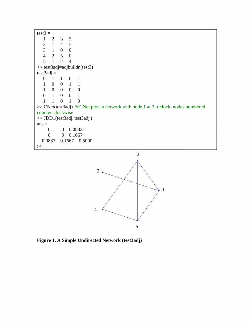
test3 = 1 2 3 5 2 1 4 5 3 1 0 0 4 2 5 0 5 1 2 4 >> test3adj=adjbuildn(test3) test3adj = 0 1 1 0 1 1 0 0 1 1 1 0 0 0 0 0 1 0 0 1 1 1 0 1 0 >> CNet(test3adj) %CNet plots a network with node 1 at 3 o’clock, nodes numbered counter-clockwise >> JDD1(test3adj,'test3adj') ans = 0 0 0.0833 0 0 0.1667 0.0833 0.1667 0.5000 >>

Figure 1. A Simple Undirected Network (test3adj)

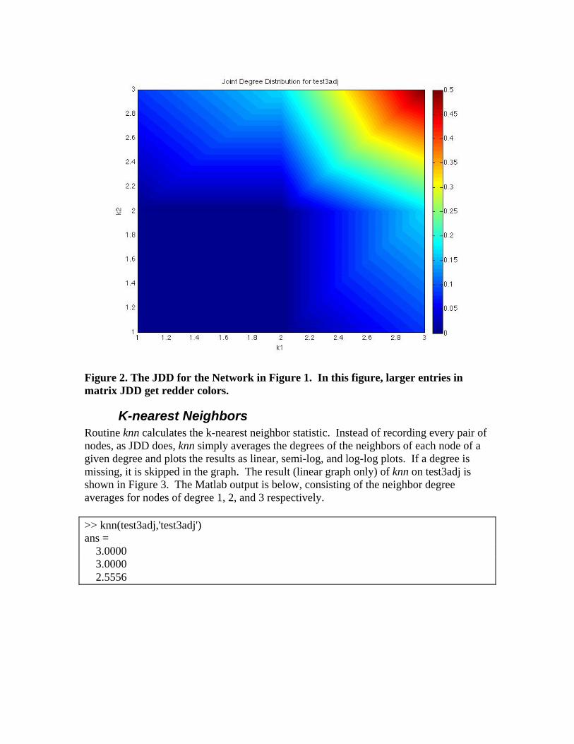
Figure 2. The JDD for the Network in Figure 1. In this figure, larger entries in matrix JDD get redder colors.

K-nearest Neighbors Routine knn calculates the k-nearest neighbor statistic. Instead of recording every pair of nodes, as JDD does, knn simply averages the degrees of the neighbors of each node of a given degree and plots the results as linear, semi-log, and log-log plots. If a degree is missing, it is skipped in the graph. The result (linear graph only) of knn on test3adj is shown in Figure 3. The Matlab output is below, consisting of the neighbor degree averages for nodes of degree 1, 2, and 3 respectively. >> knn(test3adj,'test3adj') ans = 3.0000 3.0000 2.5556

Figure 3. knn for test3adj. On average, nodes of degree = 1 link to nodes of degree = 3. The same is true for nodes of degree = 2. Nodes of degree = 3 link on average no nodes of degree = 2.55.

If knn rises as nodal degree rises, this indicates that nodes of similar degree tend to be linked, whereas if knn falls as degree rises, this indicates the opposite. In Figure 3, knn falls indicating that nodes of dissimilar degree tend to be linked.

Pearson Degree Correlation The Pearson Degree Correlation is the most condensed way to characterize the degree-link structure of a network. It consists of the conventional Pearson correlation calculation applied to each pair of linked nodes. The result always lies in the range [ with a negative result indicating that nodes of dissimilar degree tend to be linked and a positive result indicating that nodes of similar degree tend to be linked. Applying the Pearson routine to test3adj yields

−1,1]

>> Pearson(test3adj) ans = -0.2857 The three results (JDD, Knn, and Pearson for test3adj are instructive because the first one indicates that nodes of like degree tend to be linked while the second and third indicate the opposite. This discrepancy is unlikely to occur in larger networks but the user should take care. At the end of these notes, we will give an example with a large real network. Details about calculating the Pearson degree correlation are in the appendix. [Newman] calculated many statistics on 27 diverse networks and concluded that social and informational networks tended to have positive Pearson degree correlation while technological and biological networks tended to have negative Pearson degree correlation. {Alderson and Whitney] later provided data on an additional 36 networks and showed that no such pattern held. All such conclusions are subject to additional data,

but these results indicate that metrics, especially ones that condense complex patterns into small summaries, should be viewed skeptically.

Rich Club Metric Degree correlation, especially the more commonly used Pearson correlation, is often incorrectly interpreted to be an indicator of the tendency of high degree nodes to link to each other, whereas in fact it is an indicator of the tendency of similar degree nodes to link to each other. The rich club metric is specifically designed to measure the tendency of high degree nodes to link to each other. It is defined in [Colizza et al] as

Images removed due to copyright restrictions.

Earlier research by [Zhou and Mondragon] had indicated that the internet displayed a high rich club metric, implying again a central-hub structure. But high degree nodes are naturally more likely to have links with each other than do low degree nodes, so every network with a wide distribution of nodal degrees will show a positive rich club metric. Colizza et al pointed out that one needs to have a standard of comparison, so they modified their calculation to compare the result with that of a random network with the same number of nodes n and average nodal degree

, for which < k > φ(k) ~ k 2

< k > n. If a network has no more rich club tendency than a

random network then φ(k) ~ 1. Colizza et al also emphasized that the value of φ(k) is independent of the value of the Pearson degree correlation. The rich club metric can be focused on nodes of a specific value of k and higher, and measures the linking structure of just those nodes, so a counter-example with positive (that is, greater than 1) rich club metric and negative Pearson degree correlation like that in Figure 4 is easy to construct. It is likely that the rich club metric could be revised to cover a range of nodal degrees rather than just degrees greater than a given value, but that has not been done so far.

Images removed due to copyright restrictions.

Figure 4. [Colizza et al] An example network with large positive rich club metric and negative degree correlation: The highest degree nodes link maximally to each other while the lowest degree nodes link only to the highest degree ones.

Using the routine richclub on test3adj yields the following results and the graph in >> Asort=sortbyk(test3adj) Asort = 0 1 1 1 0 1 0 1 1 0 1 1 0 0 1 1 1 0 0 0 0 0 1 0 0 >> Dsort=kvec(Asort) Dsort = 3 3 3 2 1 >> [rich]=richclub(Dsort,Asort,'test3adj') rich = 1.2500 1.3223 1.3333

Figure 5. Normalized Rich Club Metric Plot for test3adj. The rising sense of this plot with consistent values grater than 1.0 indicate that there is a rich club. Inspection of the network (Figure 1) confirms this.

Network Rewiring Rewiring is a basic technique for systematically altering the structure of a network. It is not itself a metric but it can be used to change a network’s metrics. Three types of rewiring are commonly used. The first unhooks one end of an edge and randomly hooks it into a new node. The second adds edges to the network. The third swaps pairs of edges in such a way that each node retains its total edge count. Since the network’s degree sequence is thereby preserved, this method is called degree-preserving rewiring.

The first and third of these procedures can disconnect a network unless care is taken to reject rewirings that do this.

Random unhooking and rehooking is illustrated in

Figure 6. This figure shows three situations, each corresponding to a different probability p that an edge, once chosen, will be rewired, starting from the regular closed grid at the left. This method was used by Watts and Strogatz to investigate the behavior of the clustering coefficient and the average path length for different values of p . They found that values of p as small as 0.002 were sufficient to drastically reduce the average path length while at the same time the clustering coefficient was practically unchanged. They named this the “small world effect.”

Images removed due to copyright restrictions.

Figure 6. Unhooking and Rehooking [Watts and Strogatz] Randomly adding links rather than rehooking existing ones causes similar changes in network structure.

Degree-preserving rewiring was originally proposed by [Maslov and Sneppen] as a way to randomize a network. The procedure is described schematically in

Figure 7.

Images removed due to copyright restrictions.

Figure 7. Illustration of Pairwise Degree-Preserving Rewiring [Maslov and Sneppen] See also http://www.cmth.bnl.gov/~maslov/matlab.htm The first few lines of the routine sym_generate_srand are function srand=sym_generate_srand(M) %sym_generate_srand using pairwise degree-preserving rewiring srand=M; This routine takes input adjacency matrix M (stored in sparse format) and converts it to matrix srand by making 2 random pairwise rewirings, where is the number of edges in the network. The routine sym_correlation_profile compares the original network’s JDD to the randomized one’s JDD. Redder colors on the resulting graph indicate places where the original network departed significantly from a random

Ne Ne

structure. Read the short Word file in the folder “maslov rewiring stuff” or go to http://www.cmth.bnl.gov/~maslov/matlab.htm for Maslov’s own more detailed explanation.

Generating a Graph with a Specified Degree Sequence Generating a graph with a specified degree sequence, also called graph realization, is supported by a variety of methods, some of which work better than others, and some of which are at present available only for specialized degree sequences. There are two general approaches. One is to provide a specific list of the nodes and their degrees. The other is to specify a probability distribution representing a family of degree sequences with the intent that a network be generated whose degree sequence is a sample from that distribution. The simplest degree sequence to realize in a graph is the Poisson distribution because this is the distribution for a totally random graph. In such a graph, each node pair is linked with probability p . This can be done using routine randmatrix, whose text is below. function rndmat = randmatrix(n,p) %makes random matrix clear B B=sparse(n,n); for i=1:n for j=i+1:n if rand<p B(i,j)=1; end end end C=B'; D=B+C; rndmat=D; To use this routine, you provide the number of nodes you want, , and the linking probability

np . If you want the network to have a specific average nodal degree < k >,

use the following relationship:

Equation 1 < k >= z = npp = z /n

For graphs with other degree sequences or distributions, the available methods are somewhat of a scatter. They are summarized in Table 1. Function⇒ Routine or folder ⇓

Generate degree sequence from a distribution

Generate the graph from the sequence

Remarks

degree_dist

Use it to generate most distributions except power law

No First few lines of random_graph

random_graph Most distributions except power law

Yes Graph generation is slow for n > 100 - 200

erdosRenyi in folder randGraphs

Watts-strogatz grids

Yes plus a plot

Only one type of graph

sfng in folder Barabasi-Albert

Power law with 2 < k < 3 typically

As above

As above

Folder Volz

No

Generates a symmetric edge list

Can choose the clustering coeff

buildSmax

No

Builds graph with max positive degree correlation

Only one type of graph

Table 1. Summary of Routines for Generating Graphs with Specified Degree Sequences or Distributions

The routine degree_dist allows you to choose a probability distribution and a number of nodes, from which it will generate a degree sequence drawn from that distribution. You need to alter the code itself in order to alter the parameters of the distribution, such as its mean or standard deviation. This routine is part of a larger routine called random_graph, which takes the resulting degree distribution and seeks to generate the graph. This turns out to be quite slow if the network has more than a few dozen nodes. The Volz algorithm, discussed below, is much faster. Here are the first few lines of degree_dist: function [Nseq] = degree_dist(N,p,distribution,fun) % Random graph degree sequence construction routine with various models % Gergana Bounova, October 31, 2005, modified by Whitney 1-8-08 % INPUTS: % N - number of nodes % p - probability, 0<=p<=1 % distribution - probability distribution name, used below % fun - customized pr distr function, used only if distribution = % 'custom'; define the function like any other matlab function, then % call using @function_name in place of fun in the input argument % list % OUTPUTS: NSeq - degree sequence drawn from the specified distribution

Routine erdosRenyi will build a closed lattice of the type studied by Watts and Strogatz and perform the random unhooking and rehooking involved in studying the small world phenomenon. Here are the first few lines of this routine:

function [G]=erdosRenyi(nv,p,Kreg) %Function [G]=edosRenyi(nv,p,Kreg) generates a random graph based on %the Erdos and Renyi algoritm where all possible pairs of 'nv' nodes are %connected with probability 'p'. It does this by creating a connected %regular grid with k = Kreg at every node and then rewires. It does not %protect against disconnecting the network or isolating nodes. % Inputs: % nv - number of nodes % p - rewiring probability % Kreg - initial node degree of for regular graph (use 1 or even numbers) % Output: % G is a structure implemented as data structure in this as well as other % graph theory algorithms. % G.Adj - is the adjacency matrix (1 for connected nodes, 0 otherwise). % G.x and G.y - are row vectors of size nv with the (x,y) coordinates of % each node of G. % G.nv - number of vertices in G % G.ne - number of edges in G % %Created by Pablo Blinder. blinderp@bgu.ac.il

This routine is in the folder randGraphs. Included in the folder is a routine that will graph the output, called plotGraphBasic. Since the output of erdosRenyi is a data structure rather than an adjacency matrix or edge list like we are used to using, plotGraphBasic is designed to take in this datastructure. Below we discuss another graph plotting routine that takes in the adjacency matrix directly. The comments above in erdosRenyi show how to extract the adjacency matrix and the (x,y) coordinates of the nodes. Note that the comments above claim that the routine creates a random network but in fact it creates something quite different from the graphs created by randmatrix. Sample graph output from plotGraphBasic is in Figure 8.

© Pablo Blinder. All rights reserved. This content is excluded from our Creative Commons license.For more information, see http://ocw.mit.edu/fairuse.

p = 0

p = 0.35p = 0.15

p = 0.05

Figure 8. Four Sample Outputs from Routine erdosRenyi for 4 values of p. Each network has 200 nodes and parameter kreg = 4 .

Routine sfng (scale free network graph), written by Mathew Neil George, generates a degree sequence that obeys a power law. It does this by simulating the network growth process proven by Albert and Barabasi to generate power-law degree sequences, but the exponent of the power law is not possible to specify in advance. In practice it comes out in the neighborhood of -2.5. The procedure is to give the routine a small network as a seed and tell the algorithm how many edges a newly arriving node should have. The new node attaches itself according to the preferential attachment rule which says that the probability that an existing node will be chosen by an edge of the new node is proportional to the number of edges the existing node has. The routine comes with this sample of how to use it: % Here is a small example to demonstrate how to use the code. This code % creates a seed network of 5 nodes, generates a scale-free network of 300 nodes from % the seed network, and then performs the two graphing procedures. seed =[0 1 0 0 1;1 0 0 1 0;0 0 0 1 0;0 1 1 0 0;1 0 0 0 0] Net = SFNG(300, 1, seed); CNet(Net)

diagnose_matrix(Net,20) %Gergana's routine %PL_Equation = PLplot(Net) neets "fit" In this example, the seed is a simple 5-node network. The routine is called in the second line and the output network is called Net. Routine CNet plots the resulting graph. This routine will plot any network given its adjacency matrix. The last line invokes a routine that analyzes the result to see what the degree distribution is, especially to test if it follows a power law. This routine, diagnose_powerlaw, was found by ESD PhD candidate Gergana Bounova on the internet and modified by her. I have substituted it for the original routine PLplot because the latter requires a matlab routine called fit that is part of a special matlab toolkit. The result of running the sample above is as follows: seed =[0 1 0 0 1;1 0 0 1 0;0 0 0 1 0;0 1 1 0 0;1 0 0 0 0] Net = SFNG(300, 1, seed); CNet(Net) diagnose_matrix(Net,20) %Gergana's routine seed = 0 1 0 0 1 1 0 0 1 0 0 0 0 1 0 0 1 1 0 0 1 0 0 0 0 There were 300 samples generated altogether The largest sized sample is 30 Fit for power law: -2.1072x + 5.1068 Fit for log-normal: 0.71974x + 0.6654 The output says that the exponent of the power law is -2.1072. The graph produced by this routine is in Figure 9.

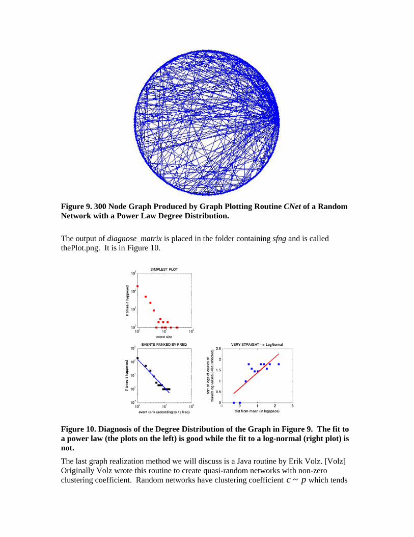
Figure 9. 300 Node Graph Produced by Graph Plotting Routine CNet of a Random Network with a Power Law Degree Distribution.

The output of diagnose_matrix is placed in the folder containing sfng and is called thePlot.png. It is in Figure 10.

Figure 10. Diagnosis of the Degree Distribution of the Graph in Figure 9. The fit to a power law (the plots on the left) is good while the fit to a log-normal (right plot) is not. The last graph realization method we will discuss is a Java routine by Erik Volz. [Volz] Originally Volz wrote this routine to create quasi-random networks with non-zero clustering coefficient. Random networks have clustering coefficient c ~ p which tends

to zero for large networks with typically small < k >. One can use degree-preserving rewiring to increase c of a random graph but it is a very slow process. (One can also raise or lower the Pearson Degree Correlation the same way and it goes much faster. Use routines rgrow and rshrink.) However, Volz’ routine can be asked to generate a network with almost zero clustering coefficient (a small bug makes the program stop if exactly zero is requested). Volz’ routine takes in a degree sequence and returns an edge list. A matlab script for using it follows. To use it, type network_generator_script. This script uses the routine degree_dist to generate the degree distribution, but you could use erdosRenyi or sfng as well if you wanted another degree distribution. Note that this routine is a Java executable, so you need a Java runtime system and library for it to work. The call to Volz’ routine is !java -jar RandomClusteringNetwork.jar degdist.txt numnodes clust_coeff resultfilename.txt The “!java -jar” at the start invokes the underlying operating system of your computer and then invokes the java runtime system. The remaining arguments are separated by spaces. The first is the name of the routine. Next is the name of the file from which the degree sequence will be read. Next is the number of nodes desired. This should be entered as a number and should be the same as the value of N in the script below. Next is the numerical value of the desired clustering coefficient, which must be a number and ≤ . Last is the name of the file into which the routine will write the symmetric edgelist of the resulting network.

> 01

The folder Volz Clustering has all the necessary routines and documentation, including Volz’ master’s thesis and a paper from Physical Review. % script to generate networks using Erik Volz' Java routine % invoke by typing graph_generation_script at the matlab command prompt % don't forget to set the desired parameters inside degree_dist first % don't forget to put the correct numerical values into the java call % !java -jar RandomClusteringNetwork.jar degdist.txt numnodes clust_coeff % edges.txt N=200 %sizenet=int16(N) [nseq] = degree_dist(N,.5,'normal'); mean_degree_seq=mean(nseq) nseqint=int16(nseq); % Volz routine requires integers input nseqabs=abs(nseqint); % protect against negative values dlmwrite('degdist.txt',nseqabs,'\t') % Volz routine requires tab delimited input file !java -jar RandomClusteringNetwork.jar degdist.txt 200 .001 edges.txt edges=dlmread('edges.txt'); % Volz routine generates a

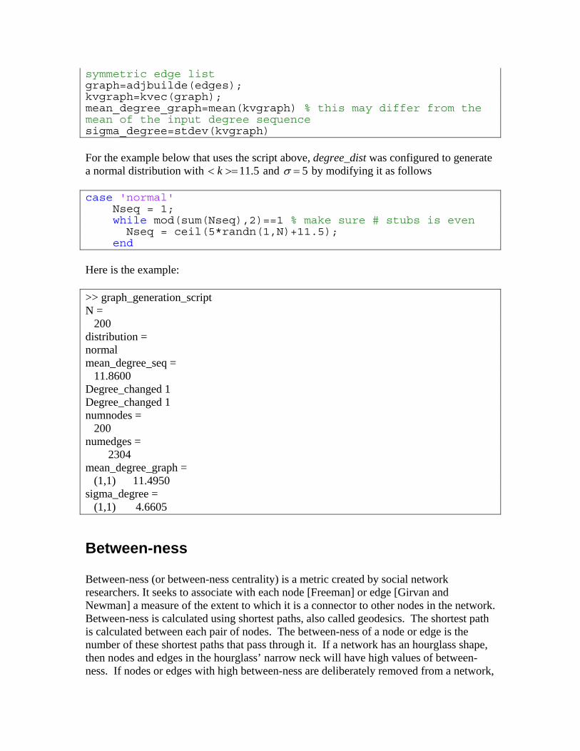
symmetric edge list graph=adjbuilde(edges); kvgraph=kvec(graph); mean_degree_graph=mean(kvgraph) % this may differ from the mean of the input degree sequence sigma_degree=stdev(kvgraph) For the example below that uses the script above, degree_dist was configured to generate a normal distribution with < k >=11.5 and σ = 5 by modifying it as follows case 'normal' Nseq = 1; while mod(sum(Nseq),2)==1 % make sure # stubs is even Nseq = ceil(5*randn(1,N)+11.5); end Here is the example: >> graph_generation_script N = 200 distribution = normal mean_degree_seq = 11.8600 Degree_changed 1 Degree_changed 1 numnodes = 200 numedges = 2304 mean_degree_graph = (1,1) 11.4950 sigma_degree = (1,1) 4.6605

Between-ness Between-ness (or between-ness centrality) is a metric created by social network researchers. It seeks to associate with each node [Freeman] or edge [Girvan and Newman] a measure of the extent to which it is a connector to other nodes in the network. Between-ness is calculated using shortest paths, also called geodesics. The shortest path is calculated between each pair of nodes. The between-ness of a node or edge is the number of these shortest paths that pass through it. If a network has an hourglass shape, then nodes and edges in the hourglass’ narrow neck will have high values of between-ness. If nodes or edges with high between-ness are deliberately removed from a network,

the network will eventually become disconnected. The resilience of a network to deliberate attack can be at least qualitatively assessed this way. This idea is also used, as discussed next, in finding communities in networks.

Finding Communities In another set of notes we discussed how to find the isolated components of a network. Each component consists of nodes linked to each other, but there are no links between components. Even if a network is completely connected, it is often true that the nodes cluster together so that nodes in a cluster tend to have more links with each other than with nodes in other clusters. Clusters are similar to modules in the sense that modules are often defined the same way: many interior mutual links and few exterior links. Researchers have come up with many ways to find communities. Since the concept is qualitative, different ways to quantify it have been proposed and evaluated. One of the most effective is that of [Girvan and Newman], which uses edge between-ness repeatedly to find the communities. The method systematically removes edges of highest between-ness and then recalculates the between-ness of the surviving edges. At some point the network breaks into two or more isolated subnetworks. The process can be repeated on each new subnetwork indefinitely, since there is no objective reason to stop. Girvan and Newman calculate a stopping metric that assesses the ratio of interior to exterior links in the network. The user of the method chooses a threshold value of the stopping criterion. UCINET contains an implementation of the Newman-Girvan algorithm along with several other community (or clique) finding methods from social network analysis. ESD PhD Mo-Han Hsieh found that the UCINET version of the Newman-Girvan algorithm occasionally gave incorrect results, so he wrote his own matlab version.

Using Mo-Han Hsieh's Newman-Girvan program Prepare a two-way symmetric edge list representing the network and store it as TEST.txt. (If you have an adjacency matrix, you can convert it to an edgelist using routine edgelist3.) Type NewmanGirvan at the matlab command prompt. The program will output intermediate results and then write three text files. The most useful of these is called dendrogramTEST. Each column of this file represents a possible partition of the network into communities. The first entry in each column is the number of communities that are not singletons themselves. The second row is the number of singletons among the communities. Note that if the routine is not told to stop at a certain number of communities, it will run until it has disintegrated the network into n communities, where n is the number of nodes. If the network is large, this could be a large number, leading to a large number of columns in this file. You can set the variable TarGroupNum to the maximum number of communities you want investigated. If

TarGroupNum = 0 then the routine will run until it has completely disintegrated the network. The third row contains the value of the stopping metric Q for each of the possible partitions. Usually the "best" partition has the largest value of Q but Q is not a sharply peaked metric so several partitions will have similar values. The remainder of each column is a list of the community numbers in which each node resides. The structure here is the same as the output of componentCount: The nodes are imagined to be listed in ascending numerical order at the left, but this obvious list is omitted. The number to the right of each node number is the number of the community it belongs to. The folder containing this routine contains an example called TEST.txt: >> type TEST.txt 1 2 1 3 1 4 1 5 2 1 2 3 3 1 3 2 4 1 4 6 5 1 5 6 6 4 6 5 This network has 6 nodes. See Figure 11.

Figure 11. Example Network TEST for Community Finding Algorithm, Showing the Two Main Communities Found

The result of typing NewmanGirvan at the matlab prompt is three output files of which the most useful is the dendrogram. Contents of output file dendrogramTEST: 0.0000000e+00 1.0000000e+00 2.0000000e+00 6.0000000e+00 3.0000000e+00 0.0000000e+00 -1.8367347e-01 4.0816327e-02 2.0408163e-01 1.0000000e+00 1.0000000e+00 1.0000000e+00 2.0000000e+00 1.0000000e+00 1.0000000e+00 3.0000000e+00 1.0000000e+00 1.0000000e+00 4.0000000e+00 2.0000000e+00 2.0000000e+00 5.0000000e+00 3.0000000e+00 2.0000000e+00 6.0000000e+00 4.0000000e+00 2.0000000e+00 There are three candidate partitions of the network, each listed in a column. Reading the first two rows together, one column at a time, we see that the first partition has no main component (zero in row 1) and instead consists of 6 isolated nodes (6 in row 2). The second has one main component and three isolates, while the third has two main components and no isolates. The third row gives Q for each of these, and this is maximum for the third column. The remaining rows contain the community numbers for the 6 respective nodes, in a format suitable for use in UCINET if you want to use Netdraw to draw the network and color the communities. In column 1 we see that each node is in its own community, numbered 1 - 6. In the second column we see that nodes 1 - 3 are in community 1 while 4 - 6 are isolates in communities 2 - 4 respectively. In column 3 we see that nodes 1 - 3 are in a community while nodes 4 - 6 are in another. This last partition is shown in Figure 11.

Examples: Random Graph and V-8 Engine First, we generate a random network with 3000 nodes and < k >= 6 using the code AA=randmatrix(3000,6/3000); Then we plot the degree sequence using figure;pds(AA,'AA') The resulting plot is in Figure 12.

Figure 12. Degree Distribution of a Random Network Then we calculate its joint degree distribution using JDD1(AA,'AA'); The resulting plot is in Figure 13.

Figure 13. JDD for Random Network

Then we calculate the k nearest neighbors statistics using knn(AA,'AA'); The results are in

Figure 14. knn for Random Network

For comparison, we do the same for a V-8 engine. The graph of this engine is in Figure 15. The input code and statistics for this network are v8=wk1read('v8 adjacency4.wk1'); >> size(v8) ans = 246 246 >> khat(v8) ans = 3.0244 >> pearson(v8) ans = -0.2688 >> clustEq3(v8) ans = 0.0318 >> clustEq5(v8) ans = 0.2118

Figure 15. Graph of V-8 Engine Next, we obtain the joint degree distribution for the -8: JDD1(v8,'V-8 Engine'); The result is in Figure 16.

Figure 16. JDD for V-8 Engine

Finally we obtain knn for the V-8: knn(v8,'V-8 Engine'); The result is in Figure 17.

Figure 17. knn for V-8 Engine. Missing marks indicate that there are no nodes with the missing degrees.

Comparing the respective plots for the random network and the V-8 engine, we see that the JDDs and knns are quite different. The random network has a fairly symmetric and broadly distributed JDD whereas the V-8 has a JDD with lots of color near opposite corners away from the diagonal. The knn for the random network is also fairly flat whereas for the V-8 it falls. This is consistent with the tendency of high degree nodes to link to lower degree nodes. Comparing the rich club metric for these networks, we get the results in Figure 18 and Figure 19. AA=full(AA); >> AAsort=sortbyk(AA); kvsortAA=kvec(AAsort); [richAA]=richclub(kvsortAA,AAsort,'AA') % note that the rich club routine will not work on sparse matrices, but randmatrix creates a sparse matrix so it must be converted to a full matrix first and

v8sort=sortbyk(v8); >> kvsortv8=kvec(v8sort); >> [rich]=richclub(kvsortv8,v8sort,'V-8 Engine');

Figure 18. Normalized Rich Club Metric for Random Matrix AA

Figure 19. Normalized Rich Club Metric for V-8 Engine The Rich Club is more or less flat for the random matrix AA but definitely falls for the V-8 indicating that there is no great tendency for the highest degree nodes to link to each other in preference to linking to lower degree nodes.

Appendix 1: Calculating Pearson Degree Correlation The formula for the Pearson degree correlation is

Equation 2 r =x − x ( ) y − y ( )∑

x − x ( )2∑ y − y ( )2∑

This is the standard form for the Pearson correlation coefficient. The x's and are the degrees of the nodes at the ends of individual links in the network, so the sums have entries, where is the number of links. If the matrix is symmetric (the graph is undirected) then there is assumed to be two links, one in each direction, between linked nodes, so the number of entries in the sums is .

y'sm

m

2m To understand the calculation, it is useful to use the Pearson function in Excel, which requires a table that is essentially an edgelist with the respective degrees of the nodes in each column. If the network has directed links, then the first column contains the degrees of source nodes and the second column contains the degrees of the destination nodes. Figure 20 shows a simple example network, whose degree correlation we will calculate using Excel.

1

2

34

5

Figure 20. Example Network for Pearson Degree Correlation Calculation Figure 21 shows the Excel screen. At the left is the edgelist table. Column A gives the node number. Each node appears as many times as it has edges. Columns B and C contain the degrees of the nodes at the ends of the edges. In the first row, since the first node is node 1, its degree (2) is in column B while the degree of the destination node is 3 for one destination and 2 for the other. x and y are the averages of the two columns of degrees, B and C respectively. The reader can verify that these averages are equal, having value 2.2. x and y will be equal for any undirected graph.

Image removed due to copyright restrictions.

Figure 21. Excel Calculation of Pearson Degree Correlation for the Network in Figure 20.

x and y can be calculated from simple network metrics < k >, the average nodal degree, and < k 2 >, the average of the squares of the nodal degrees, as follows. First,

Equation 3 x = sum of column valuesnumber of column values

To find the number of column values (the number of rows in the table), we simply note that each node of degree creates rows, so the number of rows is the sum of the degrees in the network, given by

k ksum(kvec(A)), where A is the network’s adjacency

matrix and is the matlab routine that generates the degree sequence. Thus kvec

Equation 4 number of column values= kii=1

n

∑

Since there is a k in each of k rows, the sum of the column values is simply

Equation 5 sum of column values = ki2

i=1

n

∑

Then Equation 3 becomes

Equation 6 x =ki

2

i∑

kii∑

=

1n

ki2

i=1

n

∑1n

kii=1

n

∑=< k2 >< k >

= 2.2

where we have included the numerical value that applies to the example. Note that

Equation 7 x ≥ < k >2

< k >=< k >

indicating that in general x ≠< k >. Note, too, that x is a measure of the variability in the degree sequence. We can see this by comparing Equation 6 to the coefficient of variation defined as cov =σ /μ where σ = < k 2 > − < k >2 and μ =< k >. To calculate Equation 2, we note that the numerator is essentially a quadratic form in the degree sequence and the adjacency matrix:

Equation 8 xi y j( )= xi'δij y j = x'Ax∑

where the entries xi and are the nodal degrees of linked nodes i and j respectively and superscript ‘ denotes vector or matrix transpose. The sum selects pairs of the degree

y j

sequence that represent joined nodes, a fact that is indicated by the Kronecker delta function δ ij . The selected members are multiplied together. The resulting product is equivalent to the last term on the right in Equation 8 since the adjacency matrix contains a 1 only in those places where there is a link between nodes i and j. The denominator of Equation 2 is a trivial normalization. Here is the matlab code for calculating the Pearson degree correlation function prs = pearson(A) %calculates Pearson degree correlation of A %modified 9-14-06 A=sortbyk(A); [rows,colms]=size(A); k=kvec(A); n=length(find(k~=0)); won=[ones(n,1); zeros(rows-n,1)]; %k=won'*A; ksum=won'*k'; ksqsum=k*k'; xbar=ksqsum/ksum; num=(k-won'*xbar)*A*(k'-xbar*won); kkk=(k'-xbar*won).*(k'.^.5); denom=kkk'*kkk; prs=num/denom; The modification allows for the possibility that there are isolated nodes. If the network is asymmetric (directed or mixed) use the routine pearsondir.

References [Albert and Barabasi] Barabasi, A.-L. & Albert, R. “Emergence of Scaling in Complex Networks”. Science 286, 509–512 (1999). [Colizza] V. Colizza, A. Flammini, M. A. Serrano And A. Vespignani, “Detecting Rich-Club Ordering In Complex Networks,” Nature Physics 2 February 2006, 110- 115 [Girvan and Newman] “Community Structure in Social and Biological Networks,” PNAS 99 (12) 7821 – 7826, June 11, 2002 [Li] Lun Li, David Alderson, John C. Doyle, Walter Willinger, “Towards a Theory of Scale-Free Graphs: Definition, Properties, and Implications,” Internet Mathematics,” 2 (4), 2006 [Maslov and Sneppen] S. Maslov and K. Sneppen, “Specificity and Stability in Topology of Protein Networks, Science, 296, 910 May 3 2002 [Newman] Newman, M. E. K., “The Structure and Function of Complex Networks,” SIAM Review, 45, 167–256 (2003) [Volz] “Random Networks with Tunable Degree Distribution and Clustering,” Physical Review E, 70, 056115 (2004) [Zhou and Mondragan] Zhou, S. & Mondragon, R. J., “The Rich-Club Phenomenon in the Internet Topology”. IEEE Commun. Lett. 8, 180–182 (2004).

MIT OpenCourseWarehttp://ocw.mit.edu

ESD.342 Network Representations of Complex Engineering SystemsSpring 2010 For information about citing these materials or our Terms of Use, visit: http://ocw.mit.edu/terms.