Base-Metal Potential Recognition Criteria in Study Area 2 Base-Metal Potential Recognition Criteria...

Chapter 2

Base-Metal Potential

Recognition Criteria in Study

Area

This chapter describes the application of a conceptual model of base-metal met-

allogenesis in the study area to identify deposit recognition criteria, which are

represented as predictor maps, validated using empirical spatial analyses and

subsequently used as inputs in evaluation applications of GIS-based mathemat-

ical geological models described in this research. First, tectono-stratigraphy

and base-metal mineralizations of the study area are described. Then, ex-

ploration data inputs to a GIS of the study area are described. Conjunc-

tive interpretations of processed exploration data are described next. Then,

a conceptual model of base-metal metallogenesis in the framework of overall

tectono-stratigraphic evolution of the study area is used to identify mineral-

ization controls and recognition criteria for base-metal deposits. Finally, em-

pirical models are used to validate spatial association of base-metal deposits

and the recognition criteria. Portions of this chapter have been published as

“Knowledge-driven and Data-driven Fuzzy Models for Predictive Mineral Po-

tential Mapping” (Porwal et al., 2003a) and “Tectonostratigraphy and base-

metal mineralization controls, Aravalli province (western India): new interpre-

tations from geophysical data” (Porwal et al., 2006b).

11

Base-Metal Recognition Criteria in Study Area

2.1 Study Area

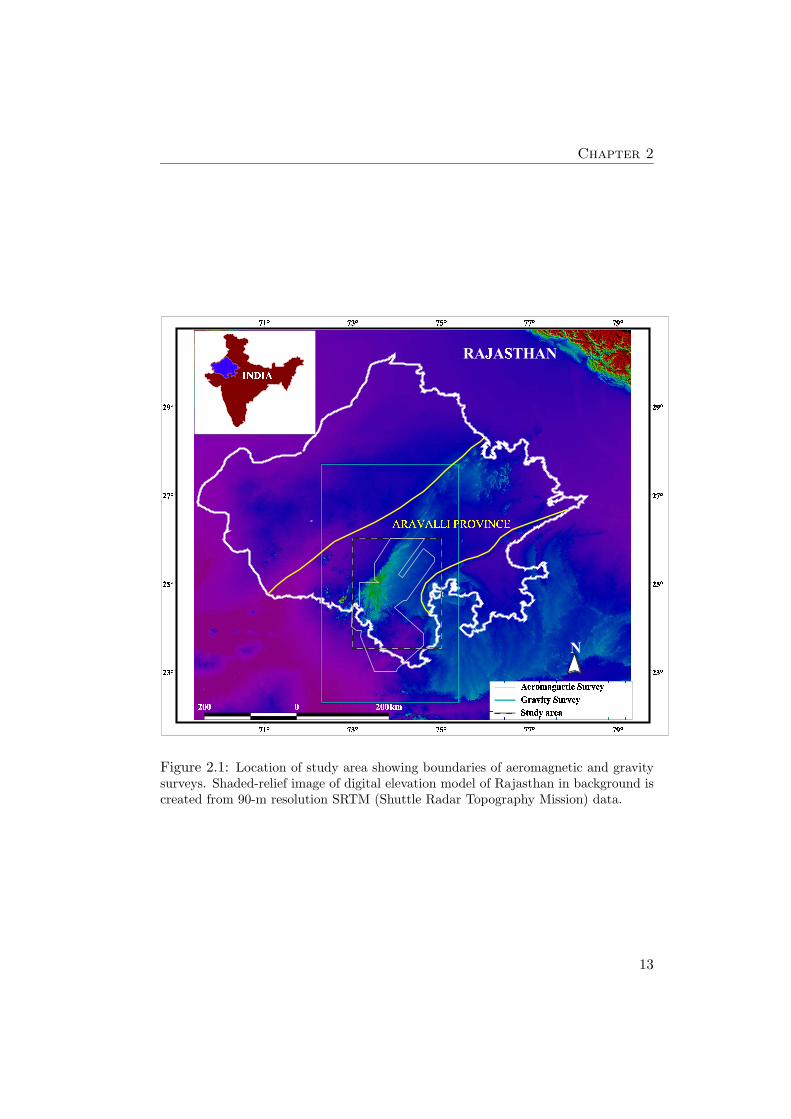
The Aravalli province (Fig.2.1), which is located in the state of Rajasthan,

India, constitutes the most important metallogenic province for base-metal

deposits in India and hosts the entire economically-viable lead-zinc resource-

base of the country. The economically-viable reserves of lead and zinc in the

province stand at 130 million tonnes with average grades of 2.2% Pb and

9.2% Zn; possible resources in producing mines and deposits under detailed

exploration amount to 30 million tonnes (Paliwal, et al., 1986; Kala, 2001;

Haldar, 2001). The province is characterized by an Archaean basement over-

lain by thick successions of intensely deformed and metamorphosed volcanic

and sedimentary rocks. Eastern parts of the province comprise flat and largely

soil-covered peneplains occupied by Archaean basement rocks. Central parts

of the province comprise the NNE-SSW trending and 700-km-long Aravalli

Mountain Chain, which is composed of Palaeo- to Meso-Proterozoic meta-

volcano-sedimentary rocks. Western parts of the province blend into the Great

Thar Desert and are occupied by Neo-Proterozoic magmatic rocks.

A block (about 50,000 km2) of the Aravalli province between latitudes

23◦30’ N and 26◦ N and longitudes 73◦ E and 75◦ E (Fig. 2.2) was selected

and used in this research as a study area for demonstrating the applications

of various mathematical geological models to mineral potential mapping. The

study area contains more than 90% of the province’s base-metal deposits plus

several base-metal prospects, occurrences and abandoned mining pits, which

have made it a prime exploration target area for base metals. It has been rel-

atively well explored by different governmental agencies. Significant amounts

of reliable and public domain data are available, largely generated by the Ge-

ological Survey of India. Moreover, genetic attributes of most of the major

deposits in the study area are documented in published literature. There-

fore, the study area meets all the assumptions stated in chapter 1 for applying

spatial-mathematical-model-based approaches to mineral potential mapping.

2.1.1 Previous geological work in study area

The broad tectono-stratigraphic framework of the study area was first defined

by Heron (1917, 1939, 1953). Since then, several field and laboratory studies

have contributed to a much better understanding of the tectono-stratigraphy of

the study area (Roy, 1988a; Gupta et al., 1997; Roy and Kataria, 1999; Sinha-

Roy et al., 1998; Deb, 2000a). Similarly, larger base-metal deposits in the

12

Chapter 2

��

��

��

��

��

��

��

��

� �

� �

��

��

��

��

��

��

��

��

!"!#!$$%&"'#%()*

Figure 2.1: Location of study area showing boundaries of aeromagnetic and gravitysurveys. Shaded-relief image of digital elevation model of Rajasthan in background iscreated from 90-m resolution SRTM (Shuttle Radar Topography Mission) data.

13


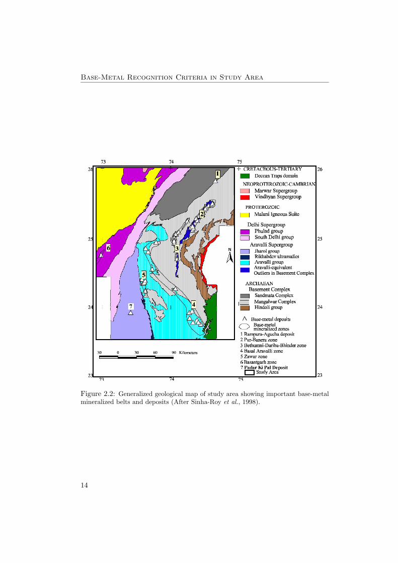
Figure 2.2: Generalized geological map of study area showing important base-metalmineralized belts and deposits (After Sinha-Roy et al., 1998).

14

Chapter 2

study area are well studied and documented (e.g., Mookherjee, 1964a, 1964b,

1965; Poddar, 1965; Straczec and Srikant, 1967; Chauhan, 1977; Gandhi et

al., 1984; Deb, 1986, 1990; Deb and Bhattacharya, 1980; Deb et al. 1989;

Ranawat et al., 1988; Sarkar, 2000; Gandhi, 2001; Haldar and Deb, 2001; Roy,

2001) and, thus, much is fairly well known about major controls on base-metal

mineralizations in the study area.

The study area is generally divided into three major tectono-stratigraphic

units (Heron, 1953; Gupta et al., 1980, 1997; Roy, 1988b).

Bhilwara supergroup. This Archaean supergroup (Raja Rao et al., 1971;

Gupta et al., 1980, 1997; Fig. 2.3A), comprising largely a heterogeneous com-

plex of granite and granodioritic gneisses, migmatites, ampbhibolites and gran-

ulites, constitutes the basement of the study area. It also contains enclaves of

meta-volcanic-sedimentary rocks (Gupta et al., 1980, 1997). Several workers

have reported remnants of greenstone sequences from the basement complex

(Sinha-Roy, 1985; Sahu and Mathur, 1991; Upadhyaya et al., 1992). The spa-

tial distribution of basement rocks in central parts of the study area (Figs. 2.3

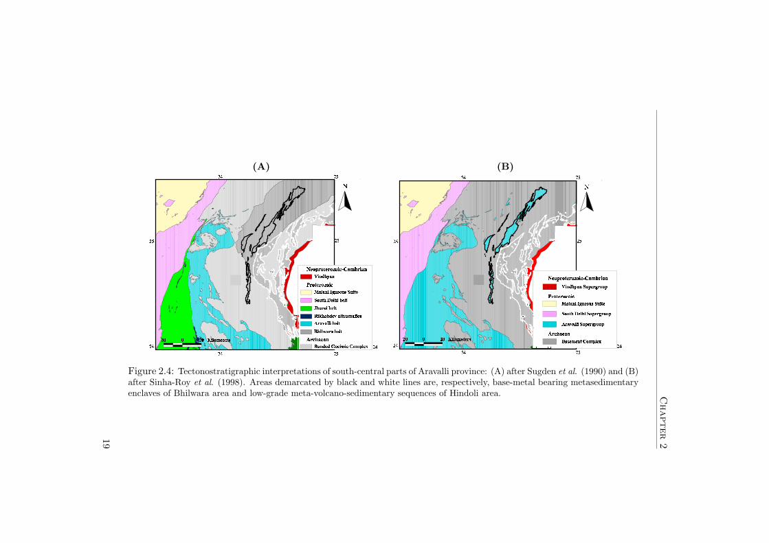
and 2.4) is ill defined and widely debated (see below). Consequently, it is re-

ferred to by various names in the literature, viz., Mewar Gneiss (Roy, 1988b,

1990; Roy and Kroner, 1996; Fig. 2.3B), Banded Gneissic Complex (Heron,

1953; Sharma, 1988; Sugden et al., 1990; Bose, 2000; Deb and Thorpe, 2001;

Fig. 2.4A) and Basement Complex (Sinha-Roy et al., 1998; Fig. 2.4B). In

spite of several commonalities, each name has a different spatial connotation

(Figs. 2.3 and 2.4).

Aravalli supergroup. This Palaeo- to Meso-Proterozoic supergroup (Figs. 2.3

and 2.4) exhibits an inverted V-shaped geometry. It is bisected roughly along

its long axis by a narrow, linearly-disposed suite of ultramafic rocks that sep-

arate a shallow-water shelf association of (predominantly dolomitic) carbon-

ates and a variety of clastic sedimentary rocks in the east from a carbonate-

free deep-water association of pelitic sediments intercalated by thin bands of

quartzites in the west (Roy and Paliwal, 1981). In southern parts of the study

area, this supergroup is separated from the basement by a profound erosional

unconformity (Roy and Paliwal, 1981; Roy et al., 1988) but, in the central

parts, the boundary between the two is blurred by a pervasive migmatization

and soil cover. The central parts comprise several linear belts of base-metal-

bearing metasedimentary sequences (outlined in black in Figs. 2.3 and 2.4) sep-

15


arated by wide tracts of gneisses and migmatites or soil cover. These metasedi-

mentary sequences host some of the largest Pb-Zn deposits of the country. The

central parts have been variously classified en bloc into the Archaean Bhilwara

supergroup (Gupta et al., 1980, 1997; Fig. 2.3A), into the Proterozoic Aravalli

supergroup (Roy, 1988b; Roy et al., 1993; Roy and Kataria, 1999; Fig. 2.3B),

or into a separate group called ‘Bhilwara belt’ of Proterozoic age (Sugden et

al., 1990; Fig. 2.4A). Sinha-Roy et al. (1998) separate these base-metal-bearing

metasedimentary enclaves from surrounding gneisses and migmatites and con-

sider the latter as parts of Archaean basement and the former as Aravalli-

equivalent Proterozoic outliers (Fig. 2.4B). The tectono-stratigraphic status

of the Hindoli volcano-sedimentary sequences along the eastern margin of the

study area (outlined in white in Figs. 2.3 and 2.4) is also unresolved. They

have been variously classified into the Archaean Bhilwara Supergroup (Gupta

et al., 1980; 1997; Fig. 2.3A), into the Proterozoic Aravalli supergroup (Roy,

1988b; Roy and Kataria, 1999; Fig. 2.3B), into the Proterozoic Bhilwara belt

(Sugden et al., 1990; Fig. 2.4A) and into the Archaean Basement Complex

(Sinha-Roy, 1988; Sinha-Roy et al., 1998; Fig. 2.4B).

Delhi supergroup. Flanking the Aravalli supergroup in the west with a

well-defined unconformity (Figs. 2.3 and 2.4), this Meso- to Neo-Proterozoic

supergroup comprises an arenite-dominated assemblage in the east and a pelite-

dominated assemblage in the west. Metavolcanic rocks have much wider tem-

poral and spatial distributions in the Delhi supergroup than in the Aravalli

supergroup. Along its western margin, the Delhi supergroup includes a suite

of base-metal-bearing volcano-sedimentary rocks (Heron, 1953; Gupta et al.,

1980; 1997; Sinha-Roy et al., 1998; Roy and Kataria, 1999) and rocks showing

ophiolitic affinity (Phulad ophiolites, cf. Gupta et al., 1980, 1997; Sugden et

al., 1990). This suite of rocks has been identified as a separate tectonic terrane

by Deb et al. (2001).

In addition to the above major tectonostratigraphic units, the study area

also contains largely undeformed and unmetamorphosed sedimentary sequences

of Neo-Proterozoic to Lower Cambrian age (Marwar and Vindhyan super-

groups; Fig. 2.2). The western parts of the study area comprise the Neo-

Proterozoic Malani Igneous Suite (Fig. 2.2), which represents a major period

of anorogenic magmatism (A-type) in the Aravalli province and forms the

third largest felsic magmatic terrane in the world (Kochar, 2000). This suite

16

Chapter 2

comprises a variety of granites and cogenetic acidic volcanic rocks showing

spectacular ring structures and radial dykes.

Base-metal mineralizations in study area

Base-metal deposits in the study area are hosted by supracrustal rocks of the

Aravalli supergroup and Delhi supergroup (Fig. 2.2). Major concentrations of

base-metal mineralization in the Aravalli supergroup occur in the Rampura-

Agucha deposit and in the Pur-Banera, Bethumni-Dariba-Bhinder and Zawar

mineralized zones (Fig. 2.2). Rampura-Agucha is a world-class Zn-Pb-(Ag) de-

posit with the highest combined metal grade (about 15%) among base-metal

deposits in India. In the Bethumni-Dariba-Bhinder zone, Zn-Pb-(Cu) deposits

are located in a 17 km long belt running from Bethumni in north to Dariba

in south, with a pyrite zone further south around Bhinder. Pur-Banera is a

low-grade polymetallic zone with several small deposits/prospects. Middle Ar-

avalli sequences host Zn-Pb deposits in the Zawar zone. In addition, low-grade

Cu(-Pb-Zn) mineralizations occur in basal sequences of the Aravalli super-

group (Fig. 2.2). The Delhi supergroup hosts smaller deposits of Cu-Zn and

Zn-Pb-Cu in the Basantgarh zone. Table 2.1 summarizes the available geolog-

ical information on important mineralized zones in the study area.

Base-metal mineralization in the study area shows systemic variation in

time and space. Broadly, the following phases of base-metal metallogeny can

be recognized.

The oldest phase is represented by low-grade dolomite-hosted Cu-(Pb-Zn)

deposits in basal sequences of the Aravalli group (Fig. 2.2). The deposits show

close spatial association with metamorphosed mafic volcanic rocks. Detailed

genetic studies on this phase of base-metal mineralization are not available.

The age of this phase of mineralization can be constrained at ca. 2000 Ma by

extrapolating available geochronological data from basal volcanic rocks (Deb

and Thorpe, 2001).

The second phase of base-metal mineralization, which has been dated at

ca. 1800 Ma (Deb and Thorpe, 2001), is represented by large SEDEX-type

Zn-Pb deposits (Menzie and Mossier, 1986; Goodfellow, 2001; Fig. 2.9B) at

Rampura-Agucha and in the Pur-Banera, Bethumni-Dariba-Bhinder and Za-

war zone of the Aravalli supergroup. Base-metal sulphide deposits in the

Aravalli-equivalent outliers (Fig. 2.2) were formed by convective seawater cir-

culation in zones of crustal extension (Deb, 1986; Deb and Sarkar, 1990). Metal

content of exhalative brines was precipitated in second-order troughs with high

17

Base-M

etal

Recognit

ion

Crit

eria

inStudy

Area

(A) (B)

+ , , + , - . / 0 1 2 3 2 4 5

6

7 87 8

7 97 9

: 8: 9

; < = > ? = @ < ? = A = B C D E F G H ? B F I

J . K L M N O K P Q R 2 4 S 4 0 Q R

T ? = @ < ? = A = B C

U O / O K . P Q . 3 2

V 2 / M . P Q R 2 4 S 4 0 Q R

W 4 O X O / / . P Q R 2 4 S 4 0 Q R

Y ? C Z F < F I[ M . / \ O 4 O P Q R 2 4 S 4 0 Q R: 8

: 9

] ^ ] _ a b c d e d f g

h

i j

k d l m f n o d g g

p d q e b o b e r d f c m a

s d q b o g e t e d u v m g d c d o e

w x y z { | { }

~ f m � m a a � t � d f � f b t �

� d a r � t � d f � f b t �

� f o � t f m m o u � d o u f m n f m o e d

� x � � | x � � � � y

� o u r � m o � t � d f � f b t �

� | � � x � � | x � � � � y � � { � � x � { }

� �

� j

i �

� �� j

i j i �

Figure 2.3: Tectonostratigraphic interpretations of south-central parts of Aravalli province: (A) after Gupta et al. (1997) and(B) after Roy (1988b). Areas demarcated by black and white lines are, respectively, base-metal bearing metasedimentary enclavesof Bhilwara area and low-grade meta-volcano-sedimentary sequences of Hindoli area.

18

Chapter

2

(A) (B)

� ��

� ��

� ��

�

� � � � � � � � � � ¡ ¢ £

¤ ¥ ¦ § ¦ © ¥ ¦ ª ¦ « ¬ ® ° ± « ²

³ � µ ¶ · ´

¹ ¦ © ¥ ¦ ª ¦ « ¬

º � � » ¼ � ½ £ ¾ ½ � ¡

¾ � ½ ¡ ¶ ¿ � ¶ � À � ¡

Á ¶ ¢ � � À � ¡

Â � Ã ¶ À µ Ä ½ � ¡ ¢ � Å � Æ £

Ç ¢ Ä � � � À � ¡

È ¶ � � É ¢ À � ¡

Ê ¬ Ë ¥ ²

È µ µ Ì � £ £ � Æ Í � � Î � Ï � �

� � Ð ÑÐ Ò

Ó ÑÓ Ñ

Ó ÒÓ Ò

Ô

Õ Ö Ö Õ Ö × Ø Ù Ú Û Ü Ý Ü Þ ß

à á â ã ä â å á ä â æ â ç è é ê ë ì í ä ç ë î

ï Ø ð ñ ò ó ô ð õ ö ÷ Ü Þ ø Þ Ú ö ÷

ù ä â å á ä â æ â ç èú ô Ù ô ð Ø û ø ð Ü Ú ö ß õ ö Ø Ý Ü

õ Ú ö Ý ò ü Ü Ù ò Ø õ ö ÷ Ü Þ ø Þ Ú ö ÷

ý Þ ô þ ô Ù Ù Ø õ ö ÷ Ü Þ ø Þ Ú ö ÷

ÿ ä è � ë á ë î� ô ß Ü Û Ü ð Ý � Ú Û ÷ Ù Ü �

Ð Ò

Ð Ñ

Figure 2.4: Tectonostratigraphic interpretations of south-central parts of Aravalli province: (A) after Sugden et al. (1990) and (B)after Sinha-Roy et al. (1998). Areas demarcated by black and white lines are, respectively, base-metal bearing metasedimentaryenclaves of Bhilwara area and low-grade meta-volcano-sedimentary sequences of Hindoli area.

19

Base-M

etal

Recognit

ion

Crit

eria

inStudy

Area

Table 2.1: Summary of available information on important mineralized zones in study area

Rampura Agucha Rajpura Dariba Pur-Banera Zawar BasantgarhDeposit Zone Zone Zone Zone

Age ∼ 1800Ma ∼ 1800 Ma ∼ 1800 Ma ∼ 1700 Ma ∼ 1000 Ma

Reserves(MT) 60 261 64 8

Combinedmetal grade(Wt%)

15.5 2.6-7.38 Low grade 6.7 9.8

Type SEDEX SEDEX SEDEX SEDEX VMS

Host lithology Graphitic micaschist withsillimanite

Recrystallizedsiliceous dolomite;carbonaceous chert;graphitic micaschists

Fine grained, greydolomite, commonlygritty/arkosic

Calc-silicates;associated bandedmagnetite quartzite

Hornblende schists;Anthophyllite-chloriteschists

Geologicalsetting

Isolatedmetasedimentaryenclave within thebasement; geologicalsequence comprisesstriped amphibolite,diopside-garnetamphibolite,graphite-garnet-mica-sillimanitegneisses, aplite,feldspathic, arkosicquartzite, pegmatite

Linear intracratonicbasins withinbasement; geologicalsequence comprisescalc biotite schistgrading torecrystallized crossbedded dolomitewith conformableamphibolite,siliceous carbonaterock, carbonaceouschert, graphite mica,banded magnetitequartzite,ferrugineous brecciain ore zone

Second order basinsclose to a basementinlier; geologicalsequence comprisesconglomerate, grit,quartzite (oftenarkosic), phyllite andgreywacke, impuredolomite

Linear intracratonicbasins withinbasement; geologicalsequence comprisescalc-silicates,hornblende schists,graphite micaschists, bandedmagnetite quartzite

Linear belts ofvolcanic rocks;geological sequencecomprisesmetamorphosed andaltered volcanicrocks (hornblende-biotite-quartz schist,cordierite-anthophyllite-sericite-quartz schist,amphibolite etc.

20

Chapter

2

Table 2.1 ContinuedRampura Agucha Rajpura Dariba Pur-Banera Zawar BasantgarhDeposit Zone Zone Zone Zone

Volcanics Amphibolite (maficvolcanics)

Amphibolites (maficvolcanics?) infootwall argillitesand tuffaceous layersin graphite micaschist

Hornblende schist None represented Metamorphosed andaltered mafic andbimodal volcanics

Organicassociation

Ubiquitous graphite Carbonaceousmatter intimatelyassociated withPb-Zn

Graphite associatedwith host rocks

Host rockscarbonaceous atplaces

None represented

Metamorphism Upper Amphibolitefacies (Maxtemperature: 650 CMax pressure : 6kbar)

Amphibolite; (Maxpressure: 5.4 kbar,Max temperature:555 C)

Amphibolite;ubiquitous evidenceof remobilization

Green schist;ubiquitous evidenceof remobilization

Amphibolite(?)

References Gandhi et al.(1984), Ranawat et

al. (1988), Deb et al.(1989), Deb andSarkar (1990),Ranawat andSharma (1990), Deband Thrope (2001),Haldar (2001), Roy(2001)

Poddar (1974),Chauhan (1977),Deb and Kumar(1982), Deb (1986),Deb et al. (1989),Deb and Sarkar(1990), Deb andThrope (2001),Haldar (2001)

Raghunandan et al.(1981); Deb andThorpe (2001)

Straczec and Srikant(1962); Deb et al.(1989), Deb andSarkar (1990), Deband Thorpe (2001)

Raghunandan et al.(1981), Deb (1999,2000b)

21


biological activity. It must be mentioned here that the Rampura-Agucha de-

posit does not show all characteristics that are typical of SEDEX deposits

(Gandhi, 2001), mainly because it has undergone high-grade metamorphism

( 700◦) that has obliterated most of the pre-metamorphic features of the de-

posit. The deposit is geologically similar to the Broken Hill deposit of Australia

for which the SEDEX model has been questioned by several authors (for ex-

ample, Plimer, 1986; Beeson, 1990; Pongratz and Davidson, 1996; Large et

al., 1996). However, Gandhi (2001) convincingly argues in favor of a SEDEX

origin of the deposit on the basis of its mineralogical composition, form and

mode of occurrence, host rock lithology and geotectonic environment. The Zn-

Pb deposits of the Aravalli group (Fig. 2.2) were formed close to a basement

inlier, in second-order basins with biological activity, by hydrothermal fluids

convecting through a heterogeneous source (Deb et al., 1989; Deb and Sarkar,

1990).

The third phase of base-metal mineralization is represented by the Zn-

Pb-Cu and Cu-Zn deposits in the Basantgarh zone of the Delhi supergroup

(Fig. 2.2). These deposits, which are associated with metamorphosed and

altered low-K tholeiites and calc-alkaline basalts, show affinity to VMS-type

deposits (Deb, 2000b). Deb and Thorpe (2001) have dated this phase of min-

eralization at ca. 1000 Ma.

2.1.2 Data requirements for further tectonostratigraphic studies

Since the pioneering works of Heron (1917, 1939, 1953), significant progress

has been made in understanding the tectono-stratigraphy of the study area.

However, as the foregoing discussion shows, the following questions (amongst

others) remain unresolved.

• Are the Hindoli sequences parts of the basement?

• What is the tectono-stratigraphic status of base-metal-bearing metased-

imentary enclaves in central parts of the study area?

• Do base-metal-bearing meta-volcanic-sedimentary sequences along the

western margin of the Delhi supergroup constitute a separate tectono-

stratigraphic domain?

Until very recently, most tectonostratigraphic studies in the study area re-

lied entirely on structural, lithological and lithogeochemical data, with very

22

Chapter 2

little consideration of geophysical data. Certain geophysical data provide in-

formation about the 3-dimensional structure of the lithosphere and can thus

provide insights into unresolved tectono-stratigraphic issues in the study area.

For example, recent deep seismic reflectivity and gravity studies over the 400-

km long Nagaur-Jhalawar transect across central parts of the Aravalli province,

carried out by the National Geophysical Research Institute (NGRI) of India,

provided a better understanding of crustal structure and tectonic evolution of

the province (Tewari et al., 1995, 1997a, 1997b, 1998, 2000; Rajendra Prasad

et al., 1998, 1999; Mishra et al., 1998, 2000; Vijaya Rao et al., 2000; Satyavani

et al., 2001).

Variations in the geomagnetic field, or magnetic anomalies, are caused by

variations in content of magnetite and other ferromagnetic minerals in crustal

rocks formed at temperatures above the Curie point (∼50 km below earth’s

surface). Magnetic anomalies thus reflect compositional and geometric varia-

tions of outcropping and concealed crustal rocks. Similarly, lateral variations

in the Earth’s gravitational field, or gravity anomalies, are essentially caused

by lateral variations of subsurface mass distribution and, therefore, reflect sub-

surface density variations. Bouguer gravity anomalies, which are determined

by applying free-air, Bouguer and terrane corrections to observed gravitational

field values (in order to eliminate effects of latitude, elevation and topography),

reflect lateral variations in density of subsurface rocks. In addition, Bouguer

gravity anomalies are, in general, useful for modeling subsurface mass distri-

butions (Bott and Hinze, 1995). Therefore, magnetic and Bouguer gravity

anomalies can provide useful insights into tectonics of a province, especially

when interpreted in conjunction with surface geological data.

In this research, conjunctive interpretations of total magnetic field inten-

sity data, Bouguer gravity data and other exploration data with the aid of a

geographic information system (GIS) are used to address the above unresolved

tectono-stratigraphic issues in the study area.

2.2 Exploration Database and Geophysical Data

Processing

Available public domain multi-disciplinary spatial data were digitized to cre-

ate a consistent regional-scale GIS of the study area that could be digitally

processed to generate (a) relevant thematic maps for conjunctive tectono-

stratigraphic and metallogenetic interpretations and (b) predictor maps for rep-

23


Table 2.2: Exploration datasets input to GIS

S.No. Dataset Scale Source Format1. Lithostratigraphic

data1:250000 Gupta et al. (1995a). Hard copy (4

sheets)

2. Structural data 1:250000 Gupta et al. (1995b). Hard copy (4sheets)

3. Base-metaldeposits data

1:250000 Raghunandan et al., (1981);DMGR (1990); In-housereports of DMGR.

Published andunpublishedtechnicalreports

4. Geochronologicaldata

- Vinogradov et al. (1964);Crawford (1970); Sivaramanand Odom (1982); Chodharyet al. (1984); Sarkar et al.

(1992); Deb et al. (1989);Wiedenbeck and Goswami(1994); Roy and Kroner(1996); Fareeduddin andKroner (1998); Wiedenbeck et

al. (1996); Deb et al. (2001);Deb and Thorpe (2001).

Publishedresearchliterature.

5. Total magneticfield intensitydata

1:250000 GSI (1981). Hard copy (4sheets ofcontour maps)

6. Bouguer gravitydata

1:1000000 Reddi and Ramakrishna(1988a).

Hard copy (1sheet ofcontour map)

resenting recognition criteria and inputting to mathematical geological models.

Datasets input to the GIS (Table 2.2) include lithostratigraphic data (Gupta

et al., 1995a), structural data (Gupta et al., 1995b), base-metal deposit/occurrence

data (from various sources), geochronological data (from various sources), total

magnetic field intensity maps (GSI, 1981) and a Bouguer gravity map (Reddi

and Ramakrishna, 1988a). Because the datasets come from diverse sources,

they were all georeferenced to the same Universal Transverse Mercator (UTM)

projection for accurate spatial data overlay.

Lithostratigraphic data

Lithostratigraphic data of the study area are available in the form of a hard-

copy or analog map (in 4 sheets on 1:250,000 scale) published by the Geolog-

ical Survey of India (Gupta et al., 1995a). The lithostratigraphic map was

synthesized from a number of regional-scale maps and relevant geological data

24

Chapter 2

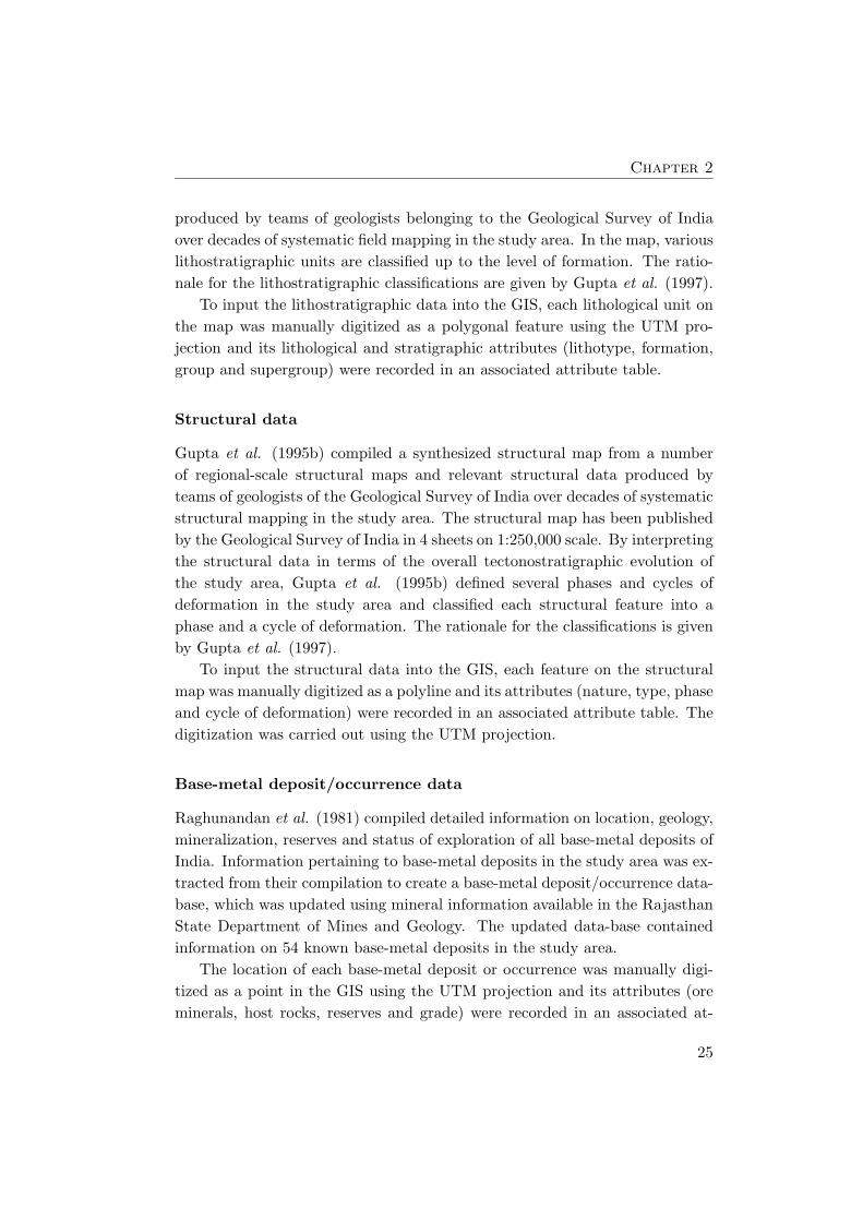
produced by teams of geologists belonging to the Geological Survey of India

over decades of systematic field mapping in the study area. In the map, various

lithostratigraphic units are classified up to the level of formation. The ratio-

nale for the lithostratigraphic classifications are given by Gupta et al. (1997).

To input the lithostratigraphic data into the GIS, each lithological unit on

the map was manually digitized as a polygonal feature using the UTM pro-

jection and its lithological and stratigraphic attributes (lithotype, formation,

group and supergroup) were recorded in an associated attribute table.

Structural data

Gupta et al. (1995b) compiled a synthesized structural map from a number

of regional-scale structural maps and relevant structural data produced by

teams of geologists of the Geological Survey of India over decades of systematic

structural mapping in the study area. The structural map has been published

by the Geological Survey of India in 4 sheets on 1:250,000 scale. By interpreting

the structural data in terms of the overall tectonostratigraphic evolution of

the study area, Gupta et al. (1995b) defined several phases and cycles of

deformation in the study area and classified each structural feature into a

phase and a cycle of deformation. The rationale for the classifications is given

by Gupta et al. (1997).

To input the structural data into the GIS, each feature on the structural

map was manually digitized as a polyline and its attributes (nature, type, phase

and cycle of deformation) were recorded in an associated attribute table. The

digitization was carried out using the UTM projection.

Base-metal deposit/occurrence data

Raghunandan et al. (1981) compiled detailed information on location, geology,

mineralization, reserves and status of exploration of all base-metal deposits of

India. Information pertaining to base-metal deposits in the study area was ex-

tracted from their compilation to create a base-metal deposit/occurrence data-

base, which was updated using mineral information available in the Rajasthan

State Department of Mines and Geology. The updated data-base contained

information on 54 known base-metal deposits in the study area.

The location of each base-metal deposit or occurrence was manually digi-

tized as a point in the GIS using the UTM projection and its attributes (ore

minerals, host rocks, reserves and grade) were recorded in an associated at-

25


tribute table.

Geochronological data

The geochronological data of radioactively-dated rocks and their locations in

the study area are available in published research literature (Vinogradov et

al., 1964; Crawford, 1970; Sivaraman and Odom, 1982; Chodhary et al., 1984;

Sarkar et al., 1989; Deb et al., 1989; Wiedenbeck and Goswami, 1994; Roy and

Kroner, 1996; Fareeduddin and Kroner, 1998; Wiedenbeck et al. 1996; Deb

et al., 2001; Deb and Thorpe, 2001). Deb and Thorpe (2001) give a detailed

synthesis and analysis of the geochronological data of the study area. The

above literature was used to create a geochronological data-base of the study

area containing locality and age data of radioactively-dated rocks.

The location of each radioactively-dated rock was manually digitized as a

point in the GIS using the UTM projection and its age was recorded in an

associated attribute table.

Total magnetic field intensity data

A large portion of the study area (Fig. 2.1) was covered by two adjacent multi-

sensor airborne magnetic surveys carried out by the United States Agency

for International Development (USAID) and the Bureau de Recherches Ge-

ologiques et Minieres/Compagnie Generale de Geophysique (BRGM/CCG).

The average flightline spacing and flight height in the case of the USAID sur-

vey were, respectively, 400 m and 60 m. The average flightline spacing and

flight height in the case of the BRGM/CCG survey were, respectively, 400 m

and 130 m. Raw data from the two surveys were processed and published

by the Geological Survey of India in two sets of total magnetic field intensity

contour maps (2 sheets for each set of data) with 10-nT contour interval (GSI,

1981).

The intersections of contours and flightlines on the total magnetic field in-

tensity maps were manually digitized into the GIS as points using the UTM

projection and the total magnetic field intensity value at each intersection point

was stored in an associated attribute table. The two sets of total magnetic field

intensity data were exported in two ASCII files using a xyz format (x and y de-

fine a co-ordinate pair for digitized magnetic value z) for processing outside the

GIS using digital techniques (see below). Images of processed total magnetic

field intensity data were input into the GIS as additional thematic layers.

26

Chapter 2

Bouguer gravity data

Bouguer gravity data of the Aravalli province are available in the form of a

contour map, with a 5 mgal contour interval, published by Geological Survey

of India (Reddi and Ramakrishna, 1988a). Areal coverage of the Bouguer

gravity data is shown in Fig. 2.1. The data are based on gravity surveys along

roads and tracks at station intervals of 2 km with elevation accuracy of 2 m

(Ramakrishna and Bhaskara Rao, 1981). The data are, therefore, regional in

nature with an overall accuracy of 1-2 mgal (Ramakrishna and Bhaskara Rao,

1981; Reddi and Ramakrishna, 1988b; Mishra et al., 2000).

The contours on the Bouguer gravity map were manually digitized into the

GIS as polylines using the UTM projection and the Bouguer gravity value of

each contour was stored in an associated attribute table. The Bouguer gravity

contours were then converted into point features and exported in ASCII files

using a xyz format (x and y define a co-ordinate pair for each Bouguer gravity

value z) for processing outside the GIS using digital techniques (see below).

Images of digitally processed Bouguer gravity data were input into the GIS as

additional thematic layers.

2.2.1 Geophysical data processing

The geophysical data were processed outside the GIS using specialized software

systems (mainly, Oasis Montaj and GM-SYS), as described below.

Total magnetic field intensity data

The two sets of total magnetic field intensity data, which were exported from

the GIS in xyz format (see above), were gridded using the minimum curvature

method (Briggs, 1974; Swain, 1976) and a cell size of 250 m. Resulting grids

were contoured automatically and then compared with original contour maps

to determine the accuracy of digital data capture. Original contour maps and

computer-generated contours maps were very similar. Subsequently, the two

grids were reduced to a common datum by upward-continuing the USAID grid

to the level at which the BRGM/CGG data was acquired.

Noise reduction. The International Geomagnetic Reference Field (IGRF)

values were removed from the grids to minimize the effect of regional mag-

netic field. Images of residual grids show several high-frequency anomalies

that appear unrelated to probable geological sources. In addition, the USAID

27


grid shows distinct NW-SE trending flightline-related noise. High-frequency

anomalies in the BRGM/CCG grid were filtered using a low-pass Butterworth

filter (k0 = 0.0005). High-frequency anomalies and flightline-related noise in

the USAID grid were suppressed by applying a combination of high-pass But-

terworth (k0 = 0.0005) and directional cosine filters (Minty, 1991). Filtering

was performed in the wavenumber domain by transforming gridded data to

wavenumbers using Fourier analysis. After filtering, the data were transformed

back to the spatial domain. The two grids were then merged and re-gridded

using the minimum curvature method and a cell size of 250 m.

Processing and visualization. To re-position magnetic anomalies over

their crustal sources, total magnetic field intensity is generally reduced to the

pole. However, at low magnetic latitudes, this process results in undesirable

amplification of N-S trending anomalies (MacLeod et al., 1993). Amplitude of

a 3D analytical signal of total magnetic field produces maxima over a magnetic

source, irrespective of direction of magnetization and, therefore, an anomaly

is re-positioned over its magnetic source without being affected by magnetic

latitude (Roest et al., 1992; MacLeod et al., 1993). Due to the low magnetic

latitude of the area, 3-D analytical signals were calculated instead of reduc-

ing total magnetic field intensity data to the pole. A first vertical derivative

(FVD) filter was applied to enhance short wavelength (near-surface) anomalies

and then the filtered data were upward-continued to various heights ranging

from 2 to 8 km to enhance long wavelength (deep-seated) anomalies. Subse-

quently, all processed magnetic grids were displayed as shaded-relief images

and then imported into the GIS to facilitate interpretation in conjunction with

the other datasets.

Bouguer gravity data

The Bouguer gravity data, which were exported from the GIS in xyz format

(see above), were gridded using the minimum curvature method and a cell size

of 2 km. The same procedure, as described above to capture aeromagnetic

data, was used to verify the accuracy of digital data capture.

Processing and visualization. The gravity data were upward-continued

to various heights ranging from 1 km to 20 km to enhance long wavelength

(deep-seated) anomalies. Using the method described by Boyce and Morris

(2002), the residual field was separated from the regional field by subtracting

28

Chapter 2

the gravity data upward-continued to 500 m from the original gravity data. A

FVD filter was then applied to the residual gravity data in order to enhance

near-surface anomalies. The processed gravity grids were displayed as shaded-

relief images to enhance anomaly features and then imported into the GIS.

2.3 Conjunctive Interpretations of Processed Data

The images of the digitally-processed geophysical data were interpreted in con-

junction with surface geological data with the aid of GIS-based overlay tech-

niques to gain insights into the tectono-stratigraphy of the study area.

Regional lineaments

Thematic layers created from the geophysical datasets show prominent regional-

scale lineaments comprising (a) composite linear to curvilinear features hav-

ing distinct characteristics from adjacent features or (b) boundaries between

crustal domains having distinct characteristics. Regional lineaments are par-

ticularly well-defined on the total magnetic field intensity image (Fig. 2.5A)

and on the FVD residual gravity image (Fig. 2.6A). Lineaments were digi-

tized from each shaded-relief image (Figs. 2.5B and 2.6B), resulting in two

new thematic layers. Magnetic lineaments show northwesterly to northeast-

erly trends and, except lineaments M6, M7 and M12, extend for more than 50

km (Fig. 2.5B). Most magnetic lineaments are discernible in the FVD resid-

ual gravity image (Fig. 2.6A), although most are indiscernible in the Bouguer

gravity image (Fig. 2.7A), perhaps due to lower resolution of the gravity data.

The FVD residual gravity image (Fig. 2.6A) shows that magnetic lineament

M15 (Fig. 2.5B) extends much further towards northeast and southwest before

changing its trend (gravity lineament G7 on Fig. 2.6B). The lineament coincides

with the western boundary of the central gravity high in the Bouguer grav-

ity image (Fig. 2.7A). Similarly, magnetic lineament M13 (Fig. 2.5B), which

coincides with gravity lineament G5 (Fig. 2.6B), extends further southwards,

swings anticlockwise and continues further east with an ENE-WSW trend. The

southern section of the lineament is discernible in the Bouguer gravity image

(Fig. 2.7A). Magnetic lineament M10 (Fig. 2.5B) is also traceable in the FVD

residual gravity image (Fig. 2.6A; G4 in Fig. 2.6B). The eastern boundary

of the central gravity high in the Bouguer gravity image (Fig. 2.7A) forms a

well-defined lineament in the FVD residual gravity image (Fig. 2.6A; G1 in

Fig. 2.6B).

29

Base-M

etal

Recognit

ion

Crit

eria

inStudy

Area

(A) (B)

� ��

� ��

� ��

� �

� � � � � � � � � � � �

� � � � � � � � � � � � � � � � ! " � � � � # � � $

% & ' ( ) * + , *

-

� ��

� �

. / /

. / 0

. / 1

. / 2

. 3

. 1

. 4

. 5

. 6

. 0

. 7. /

. 8

. / 6

9: ; < = > ? @ A ?

B C D E F G H I J H E F C K F E G L

1 2 2 1 2 M N O P Q R S R T U

. / 7

V WV XV Y

Z [Z [

Z YZ Y

Z XZ X

V YV X

V W

Figure 2.5: (A) Shaded-relief image of total magnetic field intensity and (B) interpreted lineaments.

30

Chapter

2

(A) (B)

\ ] ] \ ] ] _ a b c d e d f g

h ih i

h jh j

h kh k

l il jl kl ml h

n o p q r s t p r o u v w x t p o y v r o y t z {

| t q o } ~ v w � p v y o r �

� � � � � � � � � � � �

� � � � � � � �

� � � � � � � � �

�

l hl ml kl jl i

� � � � � � � � � � � � � � � � �

� �

� ¡� ¡

� ¢� ¢

£ £ ¡£ ¢£ ¤£ �

¥ ¦ § © ª « ¬ © ® § ® ª °

± ² ³ µ ¶ · ² ¹ º »

¼ ½ ² ³ ¶ · ²

¾ ¹ ¿ À Á ¶ ³ ² ¶

Â

Ã Ä

Ã Å

Ã ÆÃ �

Ã ÇÃ È

Ã ÉÃ �

Ã Ê

£ �£ ¤£ ¢£ ¡£

Figure 2.6: (A) Shaded-relief image of first vertical derivative of residual gravity and (B) interpreted lineaments. Crustal sectionalong transect AA’ is modeled in Fig. 2.10.

31

Base-M

etal

Recognit

ion

Crit

eria

inStudy

Area

(A) (B)

Ë Ì Ì Ë Ì Í Ì Î Ï Ð Ñ Ò Ó Ô Ó Õ Ö

× Ø× Ø

× Ù× Ù

× Ú× Ú

Û ØÛ ÙÛ ÚÛ ÜÛ ×

Ý Þ ß à ß á â ã â ä å æ ç è

é ê ë ì í î ï ð ê ñ ò ó

ô ì õ ê ë î ï ê

ö ñ ÷ ø ù î ë ê î

ú

Û ×Û ÜÛ ÚÛ ÙÛ Ø

ûü ý þ ÿ � � � � �

� � � � � � � � � ý

� � � � � � � �

� � � � � � � � � � � � �

� � � � � � � � � � � � � � � � � � ! "

# $# %# &# '# (

$ &$ &

$ '$ '

$ ($ (

) * * ) * + * , - . / 0 1 2 1 3 4

# (# '# &# %# $

Figure 2.7: Shaded-relief images of (A) Bouguer gravity data and (B) Bouguer gravity upward-continued to 20 km.

32

Chapter 2

Mafic magmatic rocks

By overlaying the lithological layer on the 3-D analytical signals layer (Fig. 2.8A),

it was found that high analytical signals coincide spatially with mapped mafic

magmatic rocks. As compared to metasedimentary and acidic magmatic rocks,

mafic magmatic rocks contain much higher concentrations of magnetite and

ferromagnesian minerals and, thus, generate stronger analytical signals. More-

over, analytical signal anomalies are positioned directly above their crustal

causative bodies. The analytical signals image (Fig. 2.8A) was thus used to in-

terpret presence of other (i.e., unmapped) mafic magmatic bodies in the area.

The interpreted mafic magmatic bodies show good spatial coincidence with

mafic magmatic bodies mapped by Gupta et al. (1995a). However, the inter-

preted mafic magmatic bodies have wider areal extents than respective mapped

mafic magmatic bodies, which indicates wider subsurface extensions of these

bodies below weakly magnetic metasedimentary rocks. Based on available in-

formation about mapped (Gupta et al., 1995a) and unmapped (Gupta et al.,

1997) mafic magmatic bodies, interpreted mafic magmatic bodies were classi-

fied as: (a) mafic metavolcanic rocks, (b) serpentinites, (c) basic granulites,

(d) norite, (e) amphibolite and (f) unclassified mafic rocks (Fig. 2.8B).

Tectonic domains

For a qualitative tectonic interpretation, the most important characteristics

of magnetic anomalies are their trends, relative amplitudes and wavelengths.

Trends of anomalies depend on orientations of magnetic sources, which, in turn,

are tectonically controlled. Wavelengths and relative amplitudes of anomalies

indicate, respectively, lateral extent and a combination of vertical extent and

relative magnetic susceptibilities of causative bodies. Together, such character-

istics of magnetic anomalies reflect the tectonic character of a crustal domain.

The magnetic image (Fig. 2.5A) was interpreted, based on anomaly character-

istics mentioned above, with the objective of dividing the area into a number

of tectonic domains (Fig. 2.9A). Due to incomplete aeromagnetic coverage, do-

mains in eastern parts of the area were demarcated based on the FVD residual

gravity image and on available tectono-stratigraphic information. The tec-

tonic domains show linear dispositions, occur as parallel or sub-parallel belts

having distinctive features in most thematic layers and show good spatial coin-

cidence with major lithostratigraphic belts identified by Sugden et al. (1990)

and Sinha-Roy et al. (1998).

33

Base-M

etal

Recognit

ion

Crit

eria

inStudy

Area

(A) (B)

5

6 7 8 9 : ; < = ;

> ? @ A B C D E F G B C H F I A B C J K L

M K E B C N B I A O E F G P F O C Q R A E O A J F E D

S T T S T U V W X Y Z [ Z \ ]

_ ^ ` ^ a^ a

b `b a

b c

d e f g h i j k e l m n

o p f q e r

b cb ab `

^ `_

s t t s t u v w x y z { z | }

~ � � � � ~ � � � � � � � � � � � �

� � � � � � � � � � � �

� � � � � ��

� � � � �

� � � �

� � � � � � � � � � �

� � � � � � � � � � � � �

¡ � ¢ � � � � � � � � � � � � � � � � � £

¤ � � � � �

� � � � � � � � � � � �

¥ � � � � � ¢ � � � � � � � � � � £

¦ §¦ ¨¦ ©

ª «ª «

ª ©ª ©

ª ¨ª ¨

¦ ©¦ ¨

¦ §

Figure 2.8: (A) Shaded-relief image of 3D analytical signals of total magnetic field intensity and (B) interpreted mafic magmaticbodies.

34

Chapter

2

(A) (B)

¬ ¬

¬ ®¬ ®

¬¬

° ° ®

°° ±

²

³ ´ µ ³ ¶ · µ ¹ ¶ º » · ¼

½ ¾ ¿ À Á Â Ã

³ Â Ä ¾ Å Æ ¾ Ç Ã À Ä È É Ê È À Å Á È Ã Ä À Ã ¿ È Ä Ë

» À Ì Â Æ ¾ Ç Ã À Ä È É ¼ Í Ì Î À Ë

¼ Ä Í Á Ë » Ì À ¾

Ï

Ð Ð ± Ð Ñ Ð Ò È Å Â Æ À Ä À Ì ¿° ±°° ®°

»

» Ó

Ô È Ã Á Õ Ë ¾ Ã Á Â Æ ¾ È Ã

º ¾ Å ¾ Ã È Á Â Æ ¾ È Ã

Ö × Ø Ù Ú Û Ü Ý Þ ß Û à á Ù â Þ Û á Ø

Ö â ã ä å æ × ç å á Ù â Þ Û á Ø

è Õ ¾ Ì Â Å Á Â Æ ¾ È Ã

é á ê å Û ß å Ù × ë Ù â Þ Û á Ø

ì ¾ È ¾ Å Â Á Â Æ ¾ È Ã

» Ì ¾ Î ¾ Å Å È Á Â Æ ¾ È Ã

í Õ È Å î ¾ Ì ¾ Á Â Æ ¾ È Ã

ï È Ã Á Â Å È Á Â Æ ¾ È Ã

¼ ¾ Ã Á Æ ¾ Ä ¾ Á Â Æ ¾ È Ã

º ¾ Ã Ç ¾ Å î ¾ Ì Á Â Æ ¾ È Ã

Figure 2.9: Tectonic domains (A) based on interpretations of magnetic data and (B) derived from geological literature. Crustalsection along transect AA’ is modeled in Fig. 2.10.

35


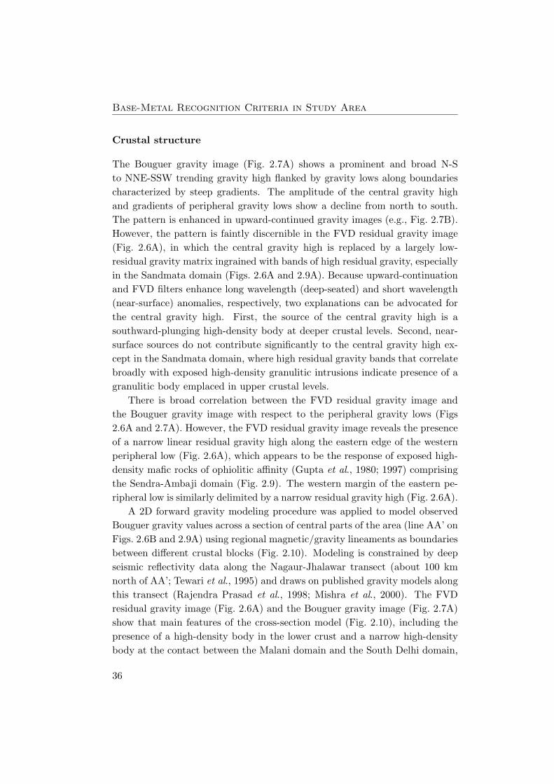
Crustal structure

The Bouguer gravity image (Fig. 2.7A) shows a prominent and broad N-S

to NNE-SSW trending gravity high flanked by gravity lows along boundaries

characterized by steep gradients. The amplitude of the central gravity high

and gradients of peripheral gravity lows show a decline from north to south.

The pattern is enhanced in upward-continued gravity images (e.g., Fig. 2.7B).

However, the pattern is faintly discernible in the FVD residual gravity image

(Fig. 2.6A), in which the central gravity high is replaced by a largely low-

residual gravity matrix ingrained with bands of high residual gravity, especially

in the Sandmata domain (Figs. 2.6A and 2.9A). Because upward-continuation

and FVD filters enhance long wavelength (deep-seated) and short wavelength

(near-surface) anomalies, respectively, two explanations can be advocated for

the central gravity high. First, the source of the central gravity high is a

southward-plunging high-density body at deeper crustal levels. Second, near-

surface sources do not contribute significantly to the central gravity high ex-

cept in the Sandmata domain, where high residual gravity bands that correlate

broadly with exposed high-density granulitic intrusions indicate presence of a

granulitic body emplaced in upper crustal levels.

There is broad correlation between the FVD residual gravity image and

the Bouguer gravity image with respect to the peripheral gravity lows (Figs

2.6A and 2.7A). However, the FVD residual gravity image reveals the presence

of a narrow linear residual gravity high along the eastern edge of the western

peripheral low (Fig. 2.6A), which appears to be the response of exposed high-

density mafic rocks of ophiolitic affinity (Gupta et al., 1980; 1997) comprising

the Sendra-Ambaji domain (Fig. 2.9). The western margin of the eastern pe-

ripheral low is similarly delimited by a narrow residual gravity high (Fig. 2.6A).

A 2D forward gravity modeling procedure was applied to model observed

Bouguer gravity values across a section of central parts of the area (line AA’ on

Figs. 2.6B and 2.9A) using regional magnetic/gravity lineaments as boundaries

between different crustal blocks (Fig. 2.10). Modeling is constrained by deep

seismic reflectivity data along the Nagaur-Jhalawar transect (about 100 km

north of AA’; Tewari et al., 1995) and draws on published gravity models along

this transect (Rajendra Prasad et al., 1998; Mishra et al., 2000). The FVD

residual gravity image (Fig. 2.6A) and the Bouguer gravity image (Fig. 2.7A)

show that main features of the cross-section model (Fig. 2.10), including the

presence of a high-density body in the lower crust and a narrow high-density

body at the contact between the Malani domain and the South Delhi domain,

36

Chapter 2

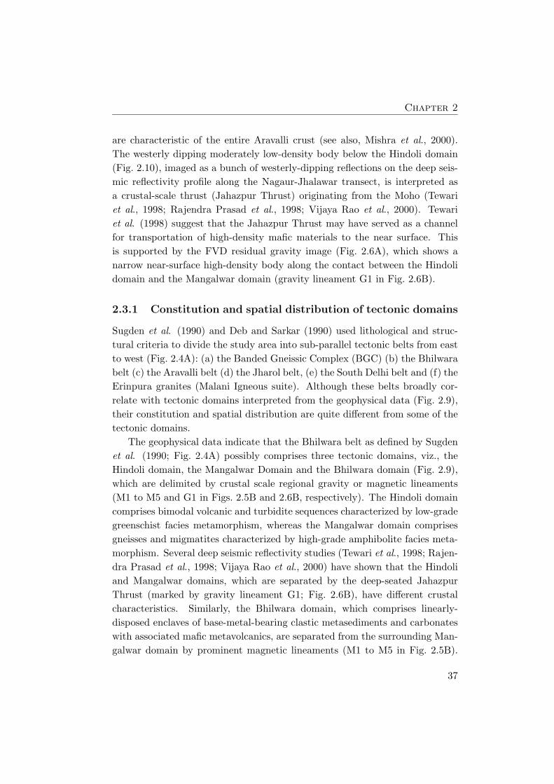
are characteristic of the entire Aravalli crust (see also, Mishra et al., 2000).

The westerly dipping moderately low-density body below the Hindoli domain

(Fig. 2.10), imaged as a bunch of westerly-dipping reflections on the deep seis-

mic reflectivity profile along the Nagaur-Jhalawar transect, is interpreted as

a crustal-scale thrust (Jahazpur Thrust) originating from the Moho (Tewari

et al., 1998; Rajendra Prasad et al., 1998; Vijaya Rao et al., 2000). Tewari

et al. (1998) suggest that the Jahazpur Thrust may have served as a channel

for transportation of high-density mafic materials to the near surface. This

is supported by the FVD residual gravity image (Fig. 2.6A), which shows a

narrow near-surface high-density body along the contact between the Hindoli

domain and the Mangalwar domain (gravity lineament G1 in Fig. 2.6B).

2.3.1 Constitution and spatial distribution of tectonic domains

Sugden et al. (1990) and Deb and Sarkar (1990) used lithological and struc-

tural criteria to divide the study area into sub-parallel tectonic belts from east

to west (Fig. 2.4A): (a) the Banded Gneissic Complex (BGC) (b) the Bhilwara

belt (c) the Aravalli belt (d) the Jharol belt, (e) the South Delhi belt and (f) the

Erinpura granites (Malani Igneous suite). Although these belts broadly cor-

relate with tectonic domains interpreted from the geophysical data (Fig. 2.9),

their constitution and spatial distribution are quite different from some of the

tectonic domains.

The geophysical data indicate that the Bhilwara belt as defined by Sugden

et al. (1990; Fig. 2.4A) possibly comprises three tectonic domains, viz., the

Hindoli domain, the Mangalwar Domain and the Bhilwara domain (Fig. 2.9),

which are delimited by crustal scale regional gravity or magnetic lineaments

(M1 to M5 and G1 in Figs. 2.5B and 2.6B, respectively). The Hindoli domain

comprises bimodal volcanic and turbidite sequences characterized by low-grade

greenschist facies metamorphism, whereas the Mangalwar domain comprises

gneisses and migmatites characterized by high-grade amphibolite facies meta-

morphism. Several deep seismic reflectivity studies (Tewari et al., 1998; Rajen-

dra Prasad et al., 1998; Vijaya Rao et al., 2000) have shown that the Hindoli

and Mangalwar domains, which are separated by the deep-seated Jahazpur

Thrust (marked by gravity lineament G1; Fig. 2.6B), have different crustal

characteristics. Similarly, the Bhilwara domain, which comprises linearly-

disposed enclaves of base-metal-bearing clastic metasediments and carbonates

with associated mafic metavolcanics, are separated from the surrounding Man-

galwar domain by prominent magnetic lineaments (M1 to M5 in Fig. 2.5B).

37


Figure 2.10: Model of crustal section along transect AA’ (Figs. 2.6B and 2.9B) basedon Bouguer gravity data. Causative sources and densities (in parenthesis; in gm/cc):1 - Vindhyan domain (2.56); 1A - high density body below Vindhyan domain (2.9);2 - Hindoli domain (2.65); 2A - high density body below Hindoli domain (2.85); 3- Mangalwar domain (2.75); 3A - Berach granite (intrusive in Mangalwar domain)(2.62); 4 - Bhilwara domain (2.72); 5 - Sandmata domain (2.76); 6 - South Delhidomain (2.72); 7 - Sendra-Ambaji domain (2.9); 8 - Malani domain (2.62); 8A - highdensity body below Malani domain (2.9); 9 - Upper Crust (2.7); 10 - high density bodywithin Lower Crust (3.04); 11 - Lower Crust (2.9); 12-Mantle (3.3). Crustal structure isconstrained by deep seismic reflectivity data along Nagaur-Jhalawar transect (about100 km north of AA’; Tewari et al., 1997). Densities of various blocks are frompublished gravity models along Nagaur-Jhalawar transect (Rajendra Prasad et al.,1998; Mishra et al., 2000). M1, M2, M8, M13 to 15 are magnetic lineaments (Fig. 2.5B.

38

Chapter 2

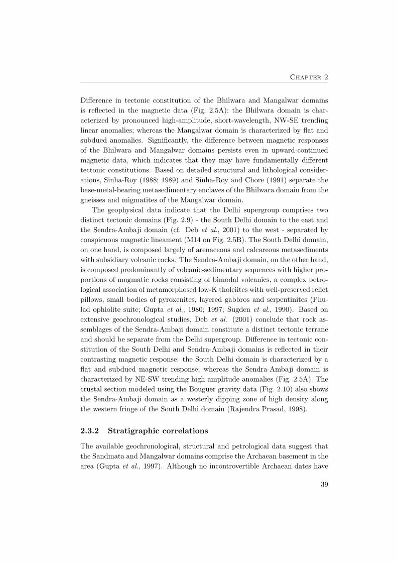
Difference in tectonic constitution of the Bhilwara and Mangalwar domains

is reflected in the magnetic data (Fig. 2.5A): the Bhilwara domain is char-

acterized by pronounced high-amplitude, short-wavelength, NW-SE trending

linear anomalies; whereas the Mangalwar domain is characterized by flat and

subdued anomalies. Significantly, the difference between magnetic responses

of the Bhilwara and Mangalwar domains persists even in upward-continued

magnetic data, which indicates that they may have fundamentally different

tectonic constitutions. Based on detailed structural and lithological consider-

ations, Sinha-Roy (1988; 1989) and Sinha-Roy and Chore (1991) separate the

base-metal-bearing metasedimentary enclaves of the Bhilwara domain from the

gneisses and migmatites of the Mangalwar domain.

The geophysical data indicate that the Delhi supergroup comprises two

distinct tectonic domains (Fig. 2.9) - the South Delhi domain to the east and

the Sendra-Ambaji domain (cf. Deb et al., 2001) to the west - separated by

conspicuous magnetic lineament (M14 on Fig. 2.5B). The South Delhi domain,

on one hand, is composed largely of arenaceous and calcareous metasediments

with subsidiary volcanic rocks. The Sendra-Ambaji domain, on the other hand,

is composed predominantly of volcanic-sedimentary sequences with higher pro-

portions of magmatic rocks consisting of bimodal volcanics, a complex petro-

logical association of metamorphosed low-K tholeiites with well-preserved relict

pillows, small bodies of pyroxenites, layered gabbros and serpentinites (Phu-

lad ophiolite suite; Gupta et al., 1980; 1997; Sugden et al., 1990). Based on

extensive geochronological studies, Deb et al. (2001) conclude that rock as-

semblages of the Sendra-Ambaji domain constitute a distinct tectonic terrane

and should be separate from the Delhi supergroup. Difference in tectonic con-

stitution of the South Delhi and Sendra-Ambaji domains is reflected in their

contrasting magnetic response: the South Delhi domain is characterized by a

flat and subdued magnetic response; whereas the Sendra-Ambaji domain is

characterized by NE-SW trending high amplitude anomalies (Fig. 2.5A). The

crustal section modeled using the Bouguer gravity data (Fig. 2.10) also shows

the Sendra-Ambaji domain as a westerly dipping zone of high density along

the western fringe of the South Delhi domain (Rajendra Prasad, 1998).

2.3.2 Stratigraphic correlations

The available geochronological, structural and petrological data suggest that

the Sandmata and Mangalwar domains comprise the Archaean basement in the

area (Gupta et al., 1997). Although no incontrovertible Archaean dates have

39


been reported from the Sandmata domain, structural and petrological consid-

erations suggest that it is a basement block that has undergone tectono-thermal

reconstitution resulting from emplacement of granulites during the Proterozoic

(Sharma, 1988; Sinha-Roy, 1988; 2001; Roy and Kataria, 1999; Bose, 2000).

In the case of the Mangalwar domain, undoubted Archaean ages have been

reported from its southern parts (MacDougall et al., 1983 1984; Gopalan et

al., 1990; Weidenbeck and Goswami, 1994; Roy and Kroener, 1996). However,

stratigraphic equivalence of southern parts with other parts of the Mangalwar

domain has been questioned strongly by Roy (1988b) and Roy and Kataria

(1999), who consider southern parts of the Mangalwar domain (∼Mewar gneiss;

cf. Roy, 1988b) as Archaean and other parts (mapped as Bhilwara belt by

Sugden et al., 1990; Fig. 2.4A) as Proterozoic. Nevertheless, based on the geo-

physical data, there seems to be absence of a definitive discontinuity between

southern and other parts of the Mangalwar domain (Figs. 2.5A, 2.6A, 2.7A

and 2.7B) and therefore the interpretation of Sinha-Roy (1988) that the Man-

galwar domain is a single block of Archaean basement rocks seems plausible.

It is pointed out, however, that the issue can only be resolved through detailed

geochronological studies.

The geochronological data indicate that the Aravalli, Bhilwara and Hin-

doli domains are Palaeo-Proterozoic and stratigraphically coeval. The age of

the Aravalli domain is constrained between ca. 2075 Ma and 2150 Ma for its

basal sequences (Deb and Thorpe, 2001) and between ca. 1690 Ma and 1710

Ma for its middle sequences (Deb et al., 1989; Deb and Thorpe, 2001); no

specific age constraints are available for its upper sequences. However, based

on indirect evidence, Sinha-Roy (2001) constrains closure of Aravalli basins

between 1500 and 1600 Ma (see also, Roy and Kataria, 1999; Deb and Thorpe,

2001). Deb and Thorpe (2001) have dated the basal sequences of the Hindoli

domain at 1854±7 Ma. The age of the Bhilwara domain is constrained at

ca. 1800 Ma based on Pb isotope data from syngenetic base-metal deposits

(Deb et al., 1989). No geochronological data are available from the Raialo do-

main. Most authors consider metasedimentary rocks of the Raialo domain as

Palaeo-Proterozoic and stratigraphically equivalent to lower Aravalli sequences

(Gupta et al., 1980, 1995a, 1997; Roy et al., 1988; Sinha-Roy, 2001). However,

Sinha-Roy et al. (1993) suggested a possibility that the Raialo rocks are parts

of the Archaean basement and are separated from the Aravalli rocks by the Ba-

nas lineament (M6 on Fig. 2.5B), which has a strong topographic expression as

well. The Banas lineament possibly does not have a deep-seated origin because

40

Chapter 2

(a) there is evidence of physical continuation of litho-units as well as magnetic

anomalies across it and (b) it does not persist in upward-continued magnetic

data. Therefore, it seems likely that the Raialo domain is Palaeo-Proterozoic

and stratigraphically coeval with the Aravalli domain.

Geochronological data are unavailable for the Jharol domain. Its strati-

graphic status is constrained mainly by field relations, which indicate that it

stratigraphically overlies the Aravalli domain (Gupta et al., 1980; 1997; Roy

et al., 1988; Sinha-Roy et al., 1998). The age of the Delhi domain is also

poorly constrained. Deb and Thorpe (2001) indicate an age of ca. 1800 Ma for

initialization of Delhi sedimentation, while Sinha-Roy (2001) suggests a much

younger age (ca. 1500). Similarly, the age of closure of Delhi basins has been

constrained variously at ca. 1400 Ma (Chodhary et al., 1984; Roy and Das,

1985), ca. 1500 (Deb and Thorpe, 2001) and at ca. 900 Ma (Sinha-Roy, 2001).

The age of the Sendra-Ambaji domain is constrained at ca. 1000 Ma by Deb

et al. (2001). Age data of the Malani domain cluster around 850 Ma.

2.4 Conceptual Model of Tectonostratigraphy and

Metallogenesis

2.4.1 Evolution of tectonic domains and base-metal mineral-

ization

Sinha-Roy (1985, 1988, 2001) and Sinha-Roy et al. (1995) postulate tectonic

evolution of Aravalli province in the framework of near-orderly Proterozoic

Wilson cycles (see also Deb and Sarkar, 1990; Sugden et al, 1990). They hy-

pothesized that recurrent phases of extensional and compressional tectonics

of the province in Proterozoic resulted in sequential opening and closing of

intracratonic rifts. Sinha-Roy (2000, 2001) described a conceptual model of

metallogenesis in the Aravalli province in the framework of the above Protero-

zoic cycles. Based on his model, evolution of the main tectonic domains and

associated base-metal mineralizations in the study area can be envisaged in

the framework of Proterozoic tectonic events as follows (Fig. 2.11).

1. At ca. 2500 Ma, the basement complex comprising the Mangalwar and

Sandmata domains was cratonized.

2. At ca. 2000 Ma, the Aravalli rift opened and, possibly through a second

phase of rifting at ca. 1800 Ma, evolved into an ocean that closed at ca.

41


Figure 2.11: Plate tectonic cartoon showing the linkage between crustal evolutionand metallogeny in study area (from Sinha-Roy, 2001).

42

Chapter 2

1500 Ma (Sinha-Roy, 2001). Synsedimentary mafic volcanics and near-

shore sediments deposited on the shelf of the Aravalli ocean constitute the

Aravalli domain, while deep-sea sediments deposited in the Aravalli ocean

constitute the Jharol domain. The Rikhabhdev domain, which com-

prises highly tectonized serpentinites, minor meta-gabbro, meta-basalt

and chert (‘Rikhabhdev ultramafics’), possibly represents an ophiolite

assemblage obducted due to closing of the Aravalli ocean (Sinha-Roy,

1984, 1988, 2000; Sugden et al., 1990; Deb and Sarkar, 1990). The first

phase of the rifting was accompanied by minor Cu(-Pb-Zn) mineraliza-

tion, while the second phase of the rifting was accompanied by a major

SEDEX-type stratabound Zn-Pb mineralization event in the Zawar zone.

The Zawar deposits were formed close to a basement inlier, in second-

order basins with biological activity, by hydrothermal fluids convecting

through a heterogeneous source comprising various sediments (Deb et al.,

1989; Deb and Sarkar, 1990).

3. At ca. 1800 Ma, several rifts opened in the Mangalwar domain accompa-

nied by mafic volcanism, possibly as pull-apart basins due to large-scale

wrench faulting associated with distensional tectonics related to the sec-

ond stage of the Aravalli rifting (Sinha-Roy, 1989; Sinha-Roy and Chore,

1991; Sinha-Roy, 2000). These narrow rifts were, however, aborted. They

are represented by linear metasedimentary enclaves in the Mangalwar do-

main and constitute the Bhilwara domain. These aborted rifts provided

favorable locales for massive SEDEX type stratabound and stratiform

Zn-Pb and Zn-Pb-Cu mineralizations at Rampura-Agucha and in the

Bethumni-Dariba-Bhinder and Pur-Banera belts, which were formed by

convective seawater circulation in zones of crustal extension (Deb, 1986;

Deb and Sarkar, 1990). Metal content of exhalative brines was precipi-

tated in second-order troughs with high biological activity.

4. At ca. 1500 Ma, the Delhi rift opened and developed into an ocean,

which was subsequently closed following subduction of Delhi ocean crust

at ca. 1000 Ma (Sinha-Roy, 2001). This resulted in formation of an island

arc along western margin of Delhi ocean, which contained VMS-type Zn-

Pb-Cu in Deri area. Subsequent closure of the back-arc basin (floored

by oceanic crust; Sinha-Roy, 2001), possibly due to a second stage of

subduction at ca. 900 Ma, resulted in obduction and emplacement of

an ophiolite melange accompanied by VMS-type Cu-Zn mineralizations

43


in the Basantgarh zone. Sediments deposited in the Delhi rift constitute

the Delhi domain, while the back-arc and island arc sequences, including

the ophiolite melange, constitute the Sendra-Ambaji domain.

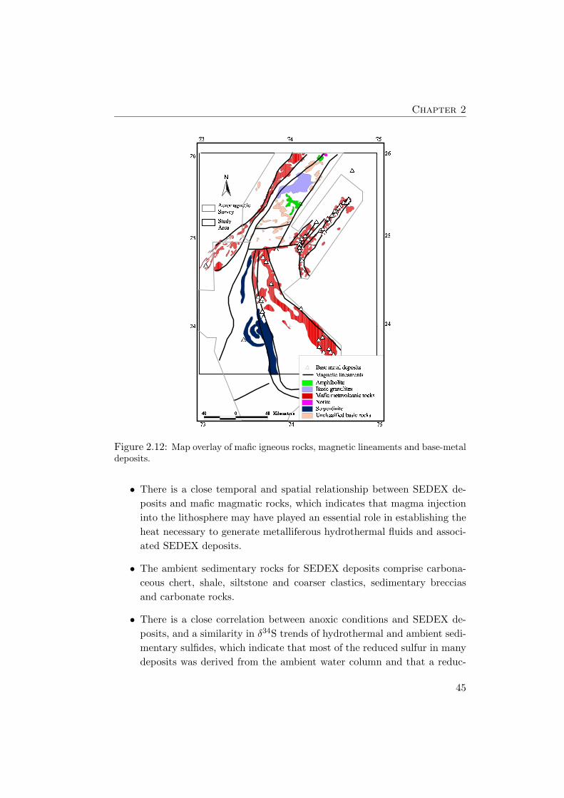
The magnetic lineaments show consistent spatial association with linear

belts of mafic magmatic bodies (Fig. 2.12). The tectonic domains delimited by

these lineaments have distinctive lithological, metamorphic and metallogenic

characteristics, which suggest that these lineaments possibly represent crustal-

scale discontinuities. This is further supported by (a) spatial coincidence of at

least some of these lineaments with established tectono-stratigraphic disconti-

nuities in the area (b) persistence of these lineaments (except Banas lineament)

in upward-continued magnetic data. In the framework of the tectonic evolution

outlined above, the magnetic lineaments are interpreted as traces of the mar-

gins of Proterozoic crustal segments (represented by tectonic domains) and,

by implication, boundaries of intracratonic rifts (the Aravalli, Bhilwara and

South Delhi domains) or subduction zones (the Sendra-Ambaji domain). As

boundaries of intracratonic rifts are generally marked by crustal scale exten-

sional faults, lineaments M1 to M5, M9 and M13 (Fig. 2.5B), which mark

boundaries of the Bhilwara, Aravalli and Delhi domains, respectively, can be

interpreted as crustal scale extensional faults. Similarly, lineaments M14 and

M15 (Fig. 2.5B), which delimit the Sendra-Ambaji domain, can be interpreted

as crustal scale (compressional?) faults.

2.4.2 Generalized geological setting of base-metal mineraliza-

tions

The conceptual model outlined above indicates that major SEDEX-type base-

metal mineralization in the study area is linked to the extensional tectonic

event at ca. 1800 Ma that resulted in (a) formation of the (aborted) Bhilwara

intracratonic rifts and (b) a second stage of rifting in the Aravalli intracratonic

rifts that led to deepening of the Aravalli ocean. The settings of the SEDEX

mineralization in the study area are similar to the following generalized setting

of SEDEX deposits (after Goodfellow, 2001, see also Fig. 2.13).

• Most SEDEX deposits are hosted by basinal sediments deposited within

failed intracratonic rifts or fault-bounded grabens or rifted continental

margins and are formed during reactivation of extensional structures.

44

Chapter 2

ðñðñðñðñðñ

ðñ

ðñ

ðñ

ðñ

ðñðñ

ðñðñðñðñðñðñðñðñðñðñ

ðñðñ

ðñ

ðñ

ðñ

ðñ

ðñ

ðñ

ðñ

ðñ

ðñ

ðñðñðñðñðñ

ðñ

ðñðñ

ðñ

ðñ

ðñðñ

ðñ

ðñ

ðñ

ðñ

ðñðñ

ðñ

ðñ

ðñ

ðñ

òóôõö÷øùú

û

÷ùøüýúþÿùó��òôø�ùö

��

��

��

��

��

��

��

��

��

��

�ÿ��ú��ùõ�ú��øü��òùø�ùÿó�ÿ�óù�üø�óù�ú��ýùóú�ü��úÿ��øü��ú��þøúÿô��óù�÷ý��ü��óù

�ú�ùýùóú�õù�ü��ó��úþÿùó��ÿùúýùÿó�

��

��

��

Figure 2.12: Map overlay of mafic igneous rocks, magnetic lineaments and base-metaldeposits.

• There is a close temporal and spatial relationship between SEDEX de-

posits and mafic magmatic rocks, which indicates that magma injection

into the lithosphere may have played an essential role in establishing the

heat necessary to generate metalliferous hydrothermal fluids and associ-

ated SEDEX deposits.

• The ambient sedimentary rocks for SEDEX deposits comprise carbona-

ceous chert, shale, siltstone and coarser clastics, sedimentary breccias

and carbonate rocks.

• There is a close correlation between anoxic conditions and SEDEX de-

posits, and a similarity in δ34S trends of hydrothermal and ambient sedi-

mentary sulfides, which indicate that most of the reduced sulfur in many

deposits was derived from the ambient water column and that a reduc-

45


Figure 2.13: Schematic section through a rift-controlled sedimentary basin showingidealized setting of SEDEX deposits. SEDEX deposits are hosted by the cover se-quence to an intracratonic rift system filled by continental clastics, marine clasticsand rift-related volcanic rocks. The rift cover sequence acts as hydrothermal caprocks (base marked by bold dashed line) to brines during their heating by deep mag-matism or burial. Geopressured heated brines flow to the contemporaneous surface ofthe cover sequence when the cap rock is ruptured by renewed extensional tectonism.(From Lydon, 1996, 2001).

ing environment may have been essential to the formation of SEDEX

deposits.

• Sedimentary textures (for example, graded and cross-laminated beds)

and other evidence suggest that most of the sulfides were deposited as

sediments on the sea floor.

The VMS-type mineralization in the Basantgarh zone of the Sendra-Ambaji

domain, on the other hand, appears to be related to compressional tectonic

events at ca. 1000, that led to the closure of Delhi rifts.

2.4.3 Mineralization controls and deposit recognition criteria

Most deposits/prospects in basal sequences of the Aravalli domain are confined

to specific stratigraphic horizons and associated with metavolcanic-dolomite-

phyllite assemblages. This indicates prominent lithological and stratigraphic

control on the first phase of base-metal mineralization. Presence of mafic

46

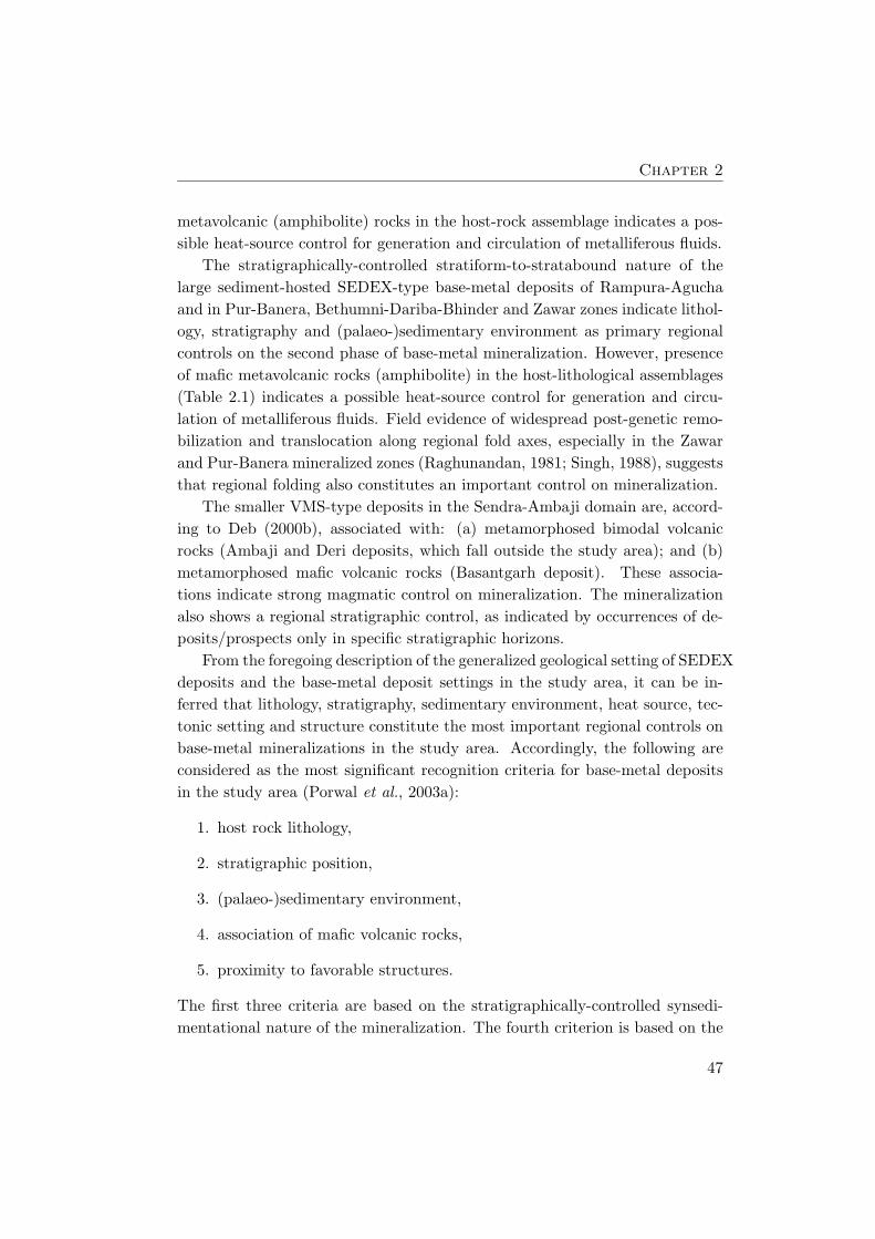
Chapter 2

metavolcanic (amphibolite) rocks in the host-rock assemblage indicates a pos-

sible heat-source control for generation and circulation of metalliferous fluids.

The stratigraphically-controlled stratiform-to-stratabound nature of the

large sediment-hosted SEDEX-type base-metal deposits of Rampura-Agucha

and in Pur-Banera, Bethumni-Dariba-Bhinder and Zawar zones indicate lithol-

ogy, stratigraphy and (palaeo-)sedimentary environment as primary regional

controls on the second phase of base-metal mineralization. However, presence

of mafic metavolcanic rocks (amphibolite) in the host-lithological assemblages

(Table 2.1) indicates a possible heat-source control for generation and circu-

lation of metalliferous fluids. Field evidence of widespread post-genetic remo-

bilization and translocation along regional fold axes, especially in the Zawar

and Pur-Banera mineralized zones (Raghunandan, 1981; Singh, 1988), suggests

that regional folding also constitutes an important control on mineralization.

The smaller VMS-type deposits in the Sendra-Ambaji domain are, accord-

ing to Deb (2000b), associated with: (a) metamorphosed bimodal volcanic

rocks (Ambaji and Deri deposits, which fall outside the study area); and (b)

metamorphosed mafic volcanic rocks (Basantgarh deposit). These associa-

tions indicate strong magmatic control on mineralization. The mineralization

also shows a regional stratigraphic control, as indicated by occurrences of de-

posits/prospects only in specific stratigraphic horizons.

From the foregoing description of the generalized geological setting of SEDEX

deposits and the base-metal deposit settings in the study area, it can be in-

ferred that lithology, stratigraphy, sedimentary environment, heat source, tec-

tonic setting and structure constitute the most important regional controls on

base-metal mineralizations in the study area. Accordingly, the following are

considered as the most significant recognition criteria for base-metal deposits

in the study area (Porwal et al., 2003a):

1. host rock lithology,

2. stratigraphic position,

3. (palaeo-)sedimentary environment,

4. association of mafic volcanic rocks,

5. proximity to favorable structures.

The first three criteria are based on the stratigraphically-controlled synsedi-

mentational nature of the mineralization. The fourth criterion is based on the

47


suggestion of Deb (1999) and Goodfellow (2001) that mafic volcanic rocks in

ore environments provided the heat necessary for the generation and circula-

tion of exhalative brines in the case of SEDEX deposits and form a significant

source of metals in the case of VMS deposits. The fifth criterion is based

on the following considerations. The extensional/compressional faults, which

mark the boundaries of the tectonic domains, could have provided structural

permeability for migration of metalliferous hydrothermal fluids. These faults

could also have focussed magmatic fluids, which, in turn, could have provided

heat-source controls for convection of hydrothermal fluids, as evidenced by

their close spatial association with mafic volcanic rocks. Furthermore, there

is a strong evidence of extensive post-genetic remobilization and relocation of

ores during subsequent deformation, especially in the Zawar and Pur-Banera

zones (Raghunandan, 1981; Singh, 1988).

It may be noticed that the recognition criteria were identified from the

SEDEX deposits, but there is some overlap of the recognition criteria of the

SEDEX and VMS type base-metal deposits (for example, association of mafic

volcanic rocks, proximity to favorable structures etc.) in the study area. As

a result, several of the mathematical models applied in this research predict

base-metal potential zones in the Sendra-Ambaji domain, which is tectonically

favorable for VMS-type base-metal mineralization (Section 2.4.1).

2.5 Empirical Models of Spatial Association of Recog-

nition Criteria with Known Base-Metal Deposits

Recognition criteria for base-metal deposits in the study area were represented

as predictor maps by processing, interpreting and/or reclassifying the explo-

ration data enumerated in Table 2.2. The procedures used are described in the

following sections. The x and y dimensions of each of the predictor map shown

in the following sections are 200 km and 275 km, respectively.

Recognition criterion 1: Host rock lithology

The lithostratigraphic map (Gupta et al., 1995a) was used to generate an ev-

idential map for the recognition criterion ‘host rock lithology.’ Irrespective

of their stratigraphic positions, all lithologies on the map were extracted to

create a map containing 136 classes of lithologies, most of which differed only

in respect of textures and/or metamorphic grades. Because this large number

48

Chapter 2

of classes would result in prohibitively large dimensionality of input data, the

map was simplified by merging the classes with similar lithological composi-

tions. The simplified map was analyzed and classes considered unrelated to

base-metal mineralizations, such as intrusive granites, trap basalt etc, were

merged to create a new class comprising lithologies unrelated to base-metal

mineralization. The reclassified map, to be used as a predictor map represent-

ing the recognition criterion ‘host rock lithology,’ is shown in Fig. 2.14A.

Recognition criterion 2: Stratigraphic position

The lithostratigraphic map (Gupta et al., 1995a) was reclassified to create an

evidential map for the recognition criterion ‘stratigraphic position.’ All strati-

graphic formations and their stratigraphic attributes (groups and supergroups)

were extracted to create a stratigraphic map of the study area. However, the

map contained 103 classes of stratigraphic formations, which would lead to un-

desirably large dimensionality of input data (see above). Therefore the map was

generalized by merging stratigraphic formations based on their stratigraphic

groups. The simplified map was analyzed and stratigraphic groups considered

unrelated to base-metal mineralizations, for example, the Vindhyan group,

Malani igneous suite, Deccan Traps, etc., were merged to create a new class

comprising stratigraphic groups not related to base-metal mineralizations. The

reclassified stratigraphic map, to be used as a predictor map representing the

recognition criterion ‘stratigraphic position,’ is shown in Fig. 2.14B.

Recognition criterion 3: (Palaeo-)sedimentary environment

A (palaeo-)sedimentary environment map of the study area is not available.

However, Gupta et al. (1997) give detailed information on mineralogy, tex-

ture, structure and interpreted depositional conditions of constituent meta-

sedimentary rocks for each stratigraphic formation. Based on this information,

the sedimentary environment of each stratigraphic formation was deduced to

generate a map representing the recognition criterion ‘(palaeo-)sedimentary

environment’ (Fig. 2.15A), which is to be used as one of the input predictor

maps. Although the number of stratigraphic formations is large, the num-

ber of classes in the map of sedimentary environments is small because many

stratigraphic formations have the same interpreted sedimentary environment.

49

Base-M

etal

Recognit

ion

Crit

eria

inStudy

Area

(A) (B)

� ! " # $ % ! % " & ' $

( ) * + , - . , / 0 1 + 2 3 4 / 0 5 3 6 7 8 3 9 / + * , /

: ; < ' ! & ' = & > ? $ ' @ ' & ! $

A % B @ & % & ' $ C B ; ' % $ $ ' $

D < E F % & % " @ ' & # E ' ! % & ' $

A B ; ' & % & ' G H < & I % & '

J > ! > @ % & ' K = > ! > @ % & % " @ < ? ! '

� ! " # $ " F % $ & K B ; ' % $ $

L L

L

L

L L

LLL

LLL

LLL

L L L

M N N M N O N P Q R S T U V U W X

Y

Z [\]\ \

\]\O

_ M _ _ ]_ ]__ M $ % " < > " a $

b b

b

b

b b

bbb

bbb

bbb

b b b

c d d c d e d f g h i j k l k m n

o

p qrsrt rt

rsre

u c u t u su su tu c

v w x y z {

| } ~ � � � � � ~ �

� w � { x �

� � y � { x � � � � z � x � � � � � x { �

� x � � x { � x y � z � � { � �

� x � � x � x � z � � { � �

� x � � � y x � � x y � � x

� � x � � � y

� x � w � � x y x

� � � x y �

Figure 2.14: Predictor map of (A) lithologies and (B) stratigraphic groups.

50

Chapter 2

Recognition criterion 4: Association of mafic volcanic rocks

An evidential map for the recognition criterion ‘association of mafic volcanic

rocks’ was generated by reclassifying the map of mafic magmatic rocks (Fig. 2.8B),

which was interpreted from total magnetic field intensity data. With the ex-

ception of the class ‘mafic meta-volcanic rocks,’ all classes on the map were

merged to create a new class comprising all mafic rocks that are not related to

base-metal mineralization in the study area. The resulting binary map of mafic

magmatic rocks, to be used as a predictor map for the recognition criterion

‘association of mafic volcanic rocks,’ is shown in Fig. 2.15B.

Recognition criterion 5: Proximity to favorable structures

As discussed in Section 2.4.3, crustal-scale faults could have played significant

role in localizing base-metal mineralizations and comprise favorable structural

locales for base-metal deposits in the study area. Because the regional mag-

netic lineaments are interpreted as defining traces of crustal-scale faults (see

Section 2.4.1), they were dilated and used as one of the predictor maps for the

recognition criteria ‘proximity to favorable structures.’ The dilation was car-

ried out by creating five buffer zones around the lineaments, each 2 km wide,

up to a distance of 10 km. A sixth zone comprising parts of the study area at

a distance greater than 10 km from the lineaments was added to generate a

predictor map of buffered distances from regional lineaments (Fig. 2.18A).

In order to identify favorable structural trends that might have controlled

localization of base-metal deposits, Fry analysis (Fry, 1979), which uses a geo-

metrical method of spatial autocorrelation for point data, was performed using

the procedure described by Vearncombe and Vearncombe (1999). For n points

there are n2 − n spatial relationships and, because of the square function, the

method yields interpretable results with small as well as large data sets.

Fry plot translations of point locations of all base metal deposits in the

study area and the corresponding rose diagram of orientations of point-to-

point translations indicate a predominant north-east trend and less dominant

north-west trend (Fig. 2.16). Figure 2.17 shows that the north-east trend is de-

fined by the major SEDEX-type base-metal deposits that formed in the second

phase of mineralization in the study area (∼ 1800 Ma metallogenetic episode),

while the north-west trend is defined by smaller deposits that formed in the

first phase of mineralization (∼ 2000 Ma metallogenetic episode).

51

Base-M

etal

Recognit

ion

Crit

eria

inStudy

Area

(A) (B)

� � � � � � �

� � � � � ¡ � ¢ � ¡ £ ¤ ¥ � � ¥ � ¦ � § � � � ¥ © ª � ¦

« ¥ © ¬ � � ¡ � ¢ � ¡ £ ¤ � � ¥ ¡ ® � � � ¥ © ª � ¦

¯ ¯

¯

¯

¯ ¯

¯¯

¯¯

¯¯

¯ ¯ ¯

° ± ± ° ± ² ± ³ µ ¶ · ¹ º »

¼

½ ¾¿À¿Á ¿Á

¿À¿²

Â ° Â Á Â ÀÂ ÀÂ ÁÂ ° « ¥ © ¬ � � ¡ � ¢ � ¡ £ ¤ ¥ � � ¥ � ¦ � § ¤ � � ¥ © ª � ¦

Ã Ä Å Æ Ç Æ È É Ê Ë Ç Ì Í Æ Î

« ¥ © ¬ � � ¡ � ¢ � ¡ £ ¤ � � � ¥ © ª � ¦

Ï Ë É Ð Æ Í Ä É Æ Ñ É Ë Ò Ä Å Æ Ç Æ É Ä Í Å

Figure 2.15: Predictor map of (A) sedimentary environments and (B) mafic magmatic rocks.

52

Chapter 2

The third phase of mineralization is represented by just one deposit in

the study area, and therefore a Fry analysis of this phase was not applicable.

Vearncombe and Vearncombe (1999) show that trends identified in Fry anal-

ysis can be used to identify the favorable structural trends for mineralization.

The above results therefore indicate that north-east and north-west are the two

favorable trends of base-metal mineralization in the study area. As discussed

in previous sections, the primary controls on base-metal mineralizations in the

study area are lithostratigraphic. Therefore, the favorable trends identified by

the Fry analysis are interpreted to indicate favorable structural trends of base-

metal-hosting lithostratigraphic units. Because trends of magnetic anomalies

reflect trends of source lithostratigraphic units, the trends of anomalies on the

shaded-relief image of the total magnetic field intensity data (Fig. 2.5A) were

mapped. A rose diagram of the lineaments thus obtained indicated four pre-

ferred orientations, viz., NE-SW, NW-SE, E-W and N-S. Based on the results

of the Fry analysis described above, the NE- and NW-trending lineaments were

extracted as separate maps and each set of lineaments was dilated by buffering

into 5 zones, each 1.5 km wide, up to a distance of 7.5 km. To these was added

a sixth zone comprising parts of the study area at a distance greater than

7.5 km from the lineaments. In this way two more predictor maps, namely,

a map of buffered distances from NE-trending lineaments (Fig. 2.18B) and a

map of NW-trending lineaments (Fig. 2.19A), were generated to represent the

recognition criterion ‘proximity to favorable structures.’

A fourth predictor map was generated by extracting regional fold axes from

the structural map of the study area (Gupta et al., 1995b). Well-documented

evidence of post-genetic remobilization and translocation of ore lenses along

regional fold axes, especially in Zawar deposits and Pur-Banera mineralized

zones, indicate that regional fold axes form favorable structural locales for

post-genetic concentration of base-metals in the study area (Raghunandan et

al., 1981; Singh, 1988; Roy, 2001). The regional fold axes were dilated by

buffering into ten zones, each 500 m wide, up to a distance of 5 km. Parts of

the study area at a distance greater than 5 km from the fold axes were classified

as the eleventh zone to generate the evidential map of buffered distances from

fold axes (Fig. 2.19B), which was used as an additional predictor map for the

recognition criterion ‘proximity to favorable structures.’

53


(A) (B)

Figure 2.16: (A) Fry plot translations (black dots) of point locations of base metaldeposits (white dots) in study area and (B) corresponding rose diagram of orientationsof point-to-point translations. Map coordinates are in meters (UTM zone 43). Petalunits of rose diagram are measured in relative frequency of orientations.

2.5.1 Spatial association with polygonal geological features

Spatial associations of known base-metal deposits and the four sets of polyg-

onal geological predictor maps, namely, lithologies, stratigraphic groups, sed-

imentary environment and mafic volcanic rocks, were tested empirically by

estimating the ratio of percentage of known deposits in a polygonal feature

to percentage of the study area occupied by the polygonal feature. This ra-

tio is indicative of conditional probability of occurrence of a base-metal de-

posit/occurrence, given the presence of a polygonal feature.

The results (Table 2.3) indicate that base-metal deposits have strong spa-

tial associations with particular lithologies (dolomite, graphitic meta-pelites,

calc-silicates and magnetite quartzite) and weak spatial associations with other

rocks. Similarly, strong spatial associations are indicated between base-metal

deposits and certain stratigraphic groups (Rajpura-Dariba, Pur-Banera, De-

bari and Nathdwara groups). Shelf sedimentary environments, especially if

characterized anaerobic conditions, show strong spatial associations with base-

metal deposits. The results also indicate a strong spatial association between

54

Chapter 2

(A) (C)

(B) (D)

Figure 2.17: Fry plot translations (black dots) of point locations of base metal de-posits (white dots) of (A) 1800 Ma metallogenic event and (B) 2000 Ma metallogenicevent, and rose diagram of orientations of point-to-point translations for (C) 1800 Mametallogenic event and (D) 2000 Ma metallogenic event. Map coordinates are in me-ters (UTM zone 43). Petal units of rose diagram are measured in relative frequencyof orientations.

55


Table 2.3: Spatial association of known base metal deposits and polygonalpredictor features

Predictor map pattern % deposits in feature% area in feature

Predictor map of lithologies1 Dolomite/dolomitic Marble 20.902 Calc-silicates 26.203 Graphic meta-pelites 28.284 Magnetite quartzite 60.965 Calc-schist/calc-gneiss 0.596 Quartzite/Arkose/Conglomerate 0.307 Migmatite/Gneisses 0.108 Not related to base metals 0.00Predictor map of stratigraphic groups1 Rajpura-Dariba group 62.332 Pur-Banera group 43.563 Debari groups 6.244 Nathdwara group 7.215 Phulad group 3.146 Udaipur group 1.367 Jharol group 0.178 Sandmata Complex 0.259 Mangalwar Complex 0.0910 Not related to base metals 0.00Predictor map of sedimentary environments1 Proximal shelf; restricted; anaerobic 22.162 Proximal shelf; anaerobic 4.233 Distal shelf; restricted; anaerobic 44.114 Proximal shelf; partly anaerobic 57.415 Deep sea 0.106 Basement Complex 0.067 Not related to base metals 0.00Predictor map of mafic igneous rocks1 Mafic volcanic rocks 99.552 Not related to base metals 2.41

base-metal deposits and mafic volcanic rocks.

The above results validate the interpretation based on a conceptual model

of base-metal metallogenesis that host rock lithology, stratigraphic position,

(palaeo-)sedimentary environment and association of mafic volcanic rocks are

important recognition criteria for base-metal deposits in the study area.

2.5.2 Spatial association with linear geological features

Using the procedures described by Bonham-Carter (1994), proximity analyses

were performed to test spatial associations of known base-metal deposits and

the four sets of predictor curvilinear features described above, namely, regional

lineaments, NE-trending lineaments, NW-trending lineaments and regional

56

Chapter

2

(A) (B)

Ó Ó

Ó

Ó

Ó Ó

ÓÓÓ

ÓÓÓ

ÓÓÓ

Ó Ó Ó

Ô Õ Õ Ô Õ Ö Õ × Ø Ù Ú Û Ü Ý Ü Þ ß

à

á âãäãå ãå

ãäãÖ

æ Ô æ å æ äæ äæ åæ Ô

ç è é ê ë

ì í î ï ð

ñ è ç ê ë

ò è ó ê ë

é è ò ê ë

ó è ô ñ ê ë

õ õ

õ

õ

õ õ

õõõ

õõõ

õõõ

õ õ õ

ö ÷ ÷ ö ÷ ø ÷ ù ú û ü ý þ ÿ þ � �

�

� ��

��

�ø� ö � � � �� ö

� � � ��

� � � � ��

Figure 2.18: Predictor map of buffered distances from (A) regional lineaments and (B) NE-trending lineaments.57

Base-M

etal

Recognit

ion

Crit

eria

inStudy

Area

(A) (B)

� �

�

�

� �

��

��

��

� � �

� � � � � � � � � ! " # $ # % &

'

( )*+

*, *,*+

*�- � - , - +- +- ,- �

. / 0 1 2 3 45 6 7 8 9 :

; 1 . / 0 3 4< / 0 1 = 3 42 1 < / 0 3 4= 1 > / 0 3 4

? @ ? A B C DE @ E A B C DE A B @ ? C D

F F

F

F

F F

FFF

FFF

FFF

F F F

G H H G H I H J K L M N O P O Q R

S

T UVW

VX VXVW

VIY G Y X Y WY WY XY G Z @ Z A B C D[ \ ] _ a

Z A B @ E C D

b A B @ B C Dc A B @ b C Db @ b A B C Dd ] ac @ c A B C Dc @ c A B C Dd ] ab @ b A B C Dc A B @ b C Db A B @ B C D

Z A B @ E C D[ \ ] _ a

Z @ Z A B C DE A B @ ? C DE @ E A B C D? @ ? A B C D

Figure 2.19: Predictor map of buffered distances from (A) NW-trending lineaments and (B) fold axes.

58

Chapter 2

fold axes. Figure 2.20 shows plots of cumulative percentage of pixels in dis-

tance corridors around the linear features and cumulative percentage of base-

metal deposit pixels in the distance corridors. The former represent random

(probability) distribution of occurrence of points (that could be occupied by

base-metal deposits) around the linear features, whilst the latter represent ob-

served distribution of base-metal deposit/occurrence points around the linear

features. Plots of the observed distribution of base-metal occurrence points

are higher than the plots of random distribution of points around the linear

feature in each case, which indicates that the probability of base-metal oc-

currence around the linear features is higher than would be expected due to

chance. The plots further indicate that base-metal deposits have a positive

spatial association with each set of linear features. The distance to linear

features in which there is highest separation between the plots represents the

distance of optimal positive spatial between base-metal occurrences and linear

geological features. Thus, the positive spatial association between base-metal

occurrences and regional lineaments is maximum at 6 km (Fig. 2.20A), the

positive spatial association between base-metal occurrences and NE-trending

lineaments is maximum at 7 km (Fig. 2.20B), the positive spatial association

between base-metal occurrences and NW-trending lineaments is maximum at

3 km (Fig. 2.20C) and the positive spatial association between base-metal oc-

currences and regional fold axes is optimal at 2 km (Fig. 2.20D). These optimal

distances of positive spatial associations depict zones around linear geological

features in which there is the highest probability for occurrence of base-metal

deposits.

The above results validate the interpretation based on a conceptual model

of base-metal metallogenesis that proximity to favorable structures forms an

important recognition criteria for base-metal deposits in the study area.

2.6 Concluding Remarks

Analysis of conjunctive interpretations of geological and geophysical datasets

vis-a-vis a review of tectono-stratigraphic studies in Aravalli province indicate

that interpreted tectonic domains, based on magnetic anomalies, have distinct

crustal, lithological, metamorphic and metallogenic characteristics and corre-

late broadly with lithostratigraphic belts identified by several earlier workers.

The analyses contribute the following new or revised interpretations to those of

earlier workers. First, Hindoli sequences probably constitute an independent

59

Base-M

etal

Recognit

ion

Crit

eria

inStudy

Area

Figure 2.20: Plots of cumulative percentage of pixels in distance corridors around linear features and cumulative percentageof base-metal occurrence pixels in distance corridors for (A) regional lineaments, (B) NE-trending lineaments, (C) NW-trendinglineaments and (D) regional fold axes.

60

Chapter 2

Palaeo-Proterozoic tectonic domain and do not form part of Archaean base-

ment complex. Second, base-metal-bearing metasedimentary enclaves in cen-

tral parts of the area also constitute an independent Palaeo-Proterozoic tec-

tonic domain, quite distinct from surrounding (basement complex?) rocks.

Third, base-metal-bearing meta-volcanic-sedimentary sequences along western

margins of Delhi supergroup constitute an independent Neo-Proterozoic tec-

tonic domain.

Based on the conceptual model of base-metal metallogenesis in the study

area and generalized geological setting of SEDEX deposits, host rock lithology,

stratigraphic position, (palaeo-)sedimentary environment, association of mafic

volcanic rocks, proximity to favorable structures are identified as significant

regional-scale recognition criteria for base-metal deposits in the study area.

Empirical modeling of spatial associations indicates strong spatial associations

between the known base-metal deposits and each recognition criterion (rep-

resented as one or more predictor maps). The empirical modeling therefore

validates the recognition criteria that were identified by conceptual modeling.

The results of the simple empirical models of spatial associations between

known base-metal deposits and each of the recognition criteria described in

this chapter can be useful in ranking or weighting the relative importance of

each predictor pattern as an indicator of base-metal deposits in the study area.

Note, however, that the simple empirical associations of known base-metal de-

posits with polygonal predictor features and with linear predictor features were

quantified in different ways. In addition, the simple empirical models presented

in this chapter do not depict spatial relationships amongst recognition criteria

with respect to the base-metal deposits. Predictive mapping of mineral poten-

tial requires (a) uniform representation of spatial associations between target

mineral deposits and recognition criteria, (b) quantitative representation of

spatial relationships amongst recognition criteria with respect to target min-

eral deposits and (c) a systematic way of combining predictor patterns that

is hypothesized to be representative of the complex process of mineral deposit

formation. These requirements can be met through complex mathematical

geological modeling. In the succeeding chapters, different mathematical geo-

logical models for weighting and combining predictor maps are developed and

evaluated by applications to base-metal potential mapping in the study area.

61

Base-Metal Potential Recognition Criteria in Study Area 2 Base-Metal Potential Recognition Criteria...

Documents

Transcript of Base-Metal Potential Recognition Criteria in Study Area 2 Base-Metal Potential Recognition Criteria...