Banking the Unbanked: What do 255 Million New Bank Accounts Reveal about Financial Access?

Sumit Agarwal

Shashwat Alok

Pulak Ghosh

Soumya Kanti Ghosh

Tomasz Piskorski

Amit Seru **

This Version: OCTOBER 2017

Abstract

Using administrative account level data, we study the largest financial inclusion program in India that led to 255 million new bank account openings. About 77% of these accounts maintain a positive balance. While the initial usage remains quite infrequent, it gradually converges to that of banked households with similar demographics. Exploiting regional variation in ex-ante financial access, we find that regions more exposed to the program saw an increase in lending and defaults on new loans. These results are consistent with banks catering to the new demand for formal credit by previously unbanked households. We also find some evidence of increased borrowing and spending for health related reasons in regions more exposed to the program.

Keywords: Banking, Financial Inclusion, Financial Literacy, Big Data, Financial Access, Savings, Spending, Debit Card, Consumer Finance, Household Finance

JLE Codes: C93; D14; G21; O16; O12

** First Version: December 2015. We would like to thank Susan Cherry, Sam Liu and Vasudha Nukala for excellent research assistance. We thank Abijit Banerjee, Thorsten Beck, Souphala Chomsisengphet, Ross Levine, Andy Rose, Bernie Yeung, Wenlan Qian and seminar participants at BIS, NUS, Reserve Bank of India, IIM-NYU Stern India Research Conference and World Bank for helpful comments and suggestions. Sam Liu and Susan Cherry provided outstanding research assistance. Corresponding Author - Agarwal: Georgetown University, ushakri@yahoo.com; Alok: Indian School of Business, shashwat_alok@isb.edu; Ghosh: Indian Institute of Management, Bangalore, pulak.ghosh@iimb.ac.in; Ghosh: State Bank of India, kantisoumya@gmail.com; Piskorski, Columbia Graduate School of Business and NBER, tp2252@columbia.edu; Seru: Stanford Graduate School of Business, Hoover Institution, SIEPR and NBER, aseru@stanford.edu.

1

I. Introduction There is a big debate about the role of financial markets and products in shaping consumer welfare and real economic activity.1 In developed economies, such as the U.S., there is an increasing discussion that the financial sector may have become inefficiently large and products offered to households may have become excessively complex.2 In contrast, in many developing countries, there has been a significant push to increase the usage of financial products – to “complete” the market (Beck et al (2008)). While there are several studies that evaluate the real effects of access to finance for firms, lack of data has meant there is limited evidence on how access to formal financial products impacts households (Dupas et al. (2016)). This paper takes a step in this direction by using micro and regional data to evaluate household usage of banking services and lending patterns around the largest financial inclusion program in the world. Our paper studies the Pradhan Mantri Jan Dhan Yojna (“JDY”) launched in India on August 28, 2014. JDY was the world’s largest financial inclusion program, with the aim to provide access to banking services for all unbanked households in India. It provided convenient access to saving accounts through a debit card and mobile banking.3 Our study has two objectives. First, we document the initial uptake (extensive margin) and subsequent usage (intensive margin) of banking services -- that includes a savings account, overdraft facilities, and insurance benefits -- by the unbanked targeted by the program. We compare the usage patterns of banking services of households who got access to banking under JDY with similar households who already had access to banking services before the program. Second, we exploit the regional variation in ex-ante financial access to explore how expanding access to financial services is related to broader outcomes such as lending, GDP growth, household spending patterns, and consumer prices. Our analysis here compares relative changes in economic outcomes in regions with greater exposure to JDY to those with lower exposure around program implementation. Financial inclusion programs can directly benefit lower income households at the micro level through savings, spending, and reduction in transaction costs. First, access to a bank account allows consumers to earn interest on their savings and provides incentives to save more. Second, savings in the bank account could help circumvent behavioural biases that would otherwise have caused them to spend this money (Benartzi and Thaler (2004), Ashraf et al (2006)). Finally, allowing access to a bank account reduces transaction costs of transferring money to

1 More than 60 countries have adopted financial inclusion as one of the key reform agendas. Financial inclusion is a key aspect of several of the United Nations sustainable development goals (2014). This thrust is driven by the fact that approximately two billion adults around the world do not have financial access. Of those who have access, approximately 40% actually use it. In India alone, there were approximately 450 million unbanked adults as of 2013 (http://rbi.org.in/Scripts/BS_SpeechesView.aspx?Id=827 [accessed on January 8th, 2016). 2 See for example Greenwood and Scharfstein (2013) and Philippon (2015). 3 Easier access is important in developing countries where formal access to bank branches may be costly due to larger distances and lack of proper infrastructure. Similar to earlier work on phone banking services for the unbanked, debit cards provide for easier access through unmanned ATMs and kiosks

2

family for subsistence and saving needs. These benefits to households notwithstanding, banks may not supply this service to such households -- in absence of a financial inclusion initiative like JDY -- for profitability reasons or due to some other frictions. Financial inclusion can also have broader regional implications through at least two channels. First, such a program could allow new capital to come into the formal banking system by means of new deposits, relaxing the capital constraints. This would allow banks to increase lending to their clients. Second, information asymmetry between new customers and lenders or other costs and frictions in acquiring new customers may imply that a program like JDY may allow banks to meet the demand for credit for some households that previously operated outside of the formal banking sector. To the extent that this increase in credit is large, one would see such programs stimulating local economic growth through increased consumption, investments, and employment. Our micro level analysis relies on proprietary micro level data on a random sample of approximately 1.5 million accounts opened under JDY during August 2014 to May 2015 by one of the largest banks in India. This allows us to capture the usage of banking services during the first ten months of the program. This bank is one of the largest Indian banks based on deposit and lending base. In addition, we obtain data from the same bank on two distinct comparison groups: (i) around 50 thousand regular accounts of individuals broadly similar to JDY households opened during the same period (“non-JDY” accounts) and, for robustness, (ii) around 1 million accounts for low-income individuals -- with similar demographic profile like JDY households – opened just prior to the program and tracked over the same time period (“pre-JDY” accounts). This dataset provides us with precise account level information on monthly account balance, withdrawal, deposit, inward and outward remittance transactions, along with demographic information on the consumers. We also supplement this data with regional and aggregate statistics provided by the central bank, which is available to us over a longer time period (till November 2016). We begin by documenting substantial outreach of the program (i.e., the extensive margin). In particular, the program led to a large increase in the number of households having access to the formal banking services. The number of accounts steadily increased at a rate of 14% new accounts per month since the start of the program. As of Nov 11, 2016 we find 255 million new accounts and 190 million debit cards issued under JDY. Moreover, 77% of the accounts maintain some positive balance. These facts are consistent with those obtained by using the micro data from our bank and extrapolating the estimates to national level over the longer horizon. We also find that the average monthly balance maintained in JDY accounts is INR 482 (USD 7)4 or about 60% of the rural poverty line in India.

4 INR 482 translates into USD 7 at the current nominal exchange rate of INR68 per USD. On a PPP basis this translates into USD 23.

3

Along the intensive margin, we find that approximately 81% of the new consumers do not deposit any money after account opening in the first six months since the account opening. About 12% of individuals perform one deposit transaction while only 7% perform two or more deposit transactions. The statistics are qualitatively similar for cash withdrawals, with approximately 87% of the sample not withdrawing any cash after opening the account, about 5% withdrawing cash only once and 8% withdrawing cash two or more times. In terms of types of transactions done by households banked under JDY, inward and outward remittances are the most common transactions. Approximately 34% (21%) of individuals receive (send) money in their account via inward (outward) remittance during the first six months since the account opening. Examining the frequency of transactions, we find that 17% (15%) of individuals receive (send) inward (outward) remittance only once during our sample period, while about 17% (8%) receive (send) remittance two or more times. The percentage of heavy users performing such transactions – i.e., those performing such transactions more than once a month -- is extremely low at less than 1%. Overall, our micro-evidence suggests that there was substantial uptake by households under JDY. Moreover, both savings and transactions go up over time for individuals that are banked under the program. This evidence is consistent with learning by individuals that results in an increase in usage over time as they gain familiarity with banking services. The initial usage is quite infrequent and concentrated among a subset of the consumers with stronger intensity among married account holders. We next compare the account activity of JDY households to similar households that were banked without direct government intervention (pre-JDY and non-JDY households). We find that the usage patterns under the program gradually converge over time to those of similar individuals who were banked outside the program. Our estimates suggest this convergence occurs on average within six to twelve months since an account opens. We note that these micro effects are established using a limited time series. Thus, longer time series data is needed to evaluate the long-run validity of these facts. Next, we exploit spatial (regional) variation in implementation of this program to investigate how access to consumer savings accounts is related to broader economic outcomes such as lending and local GDP growth. To do this, we construct four ex-ante measures of JDY program exposure: (i) number of adults per unit bank branch in a region – this captures the extent of bank branch penetration, (ii) fraction of bank branches owned by state-owned banks in a region -- since privately owned banks are more likely to open branches in higher income areas with greater financial inclusion, (iii) fraction of unbanked households in a region – this captures the extant level of banking access in each area and (iv) a comprehensive financial inclusion index

4

obtained from CRISIL 5 that uses three parameters as inputs to the index: bank branch penetration, deposit penetration and credit penetration. A higher value of all four measures indicates a lower level of financial inclusion. We compare changes in the regional outcome variables in regions with greater ex-ante program exposure relative to regions with lower program exposure around program implementation. We begin our regional analysis by verifying that our ex-ante measures of regional JDY exposure in a region before the program indeed correlate with the subsequent intensity of treatment from the program. We observe that there is a strong positive association between our ex-ante exposure measures with both the number of JDY accounts opened and the total amount deposited in these accounts. Next, we examine whether JDY is associated with an increase in bank lending. In districts with high ex-ante exposure to JDY, using aggregate data provided by the central bank of India, we observe an increase in aggregate lending in areas with greater ex-ante JDY exposure. We verify these effects are present in our micro data and find an increase in both the number of new loans granted and the amount of loans granted in regions with greater JDY exposure relative to those with lower exposure. We find that the total amount of new deposits brought under JDY is small relative to overall deposits in the banks before the program. In particular, the INR 460 billion deposited in JDY accounts is a mere 0.06% of the pre-JDY deposits in the banking sector. Thus, it is unlikely that the additional lending in more exposed regions solely reflects a relaxation of bank financial constraints due to new deposit inflow. Rather, our findings suggest that JDY may have allowed banks to meet the unmet demand for credit for some households that did not have prior access to formal banking products. Next, we we use data from a time-series panel of household survey conducted by Centre for Monitoring Indian Economy (CMIE) and examine the association between ex-ante exposure to JDY with the sources and reasons for borrowing, household savings and consumption. Focusing on the low-income households defined as those with below median monthly income in our sample, we find that consistent with the findings based on bank data, there is an increase in the fraction of households borrowing from banks in regions with greater ex-ante JDY exposure relative to regions with lower exposure. We also observe a contemporaneous decrease in the fraction of households borrowing from non-bank sources such as informal moneylenders, chit funds, friends, and family, etc. To the extent that many of these informal creditors engage in predatory loan pricing, this evidence is consistent with the thesis that households may prefer to substitute these arguably costly sources of credit with bank credit whenever possible. With regards to the purpose of households’ borrowing from banks, we find some evidence of increased borrowing to fund the medical expenditure needs. Next, we examine the association between JDY exposure and household savings and consumption patterns at the regional level. First, we find a relative increase in the fraction of 5 CRISIL is a global analytical company providing Ratings, Research and Risk & Policy Advisory services.

5

households that intend to start saving in more exposed areas. Second, consistent with an increase in the fraction of households borrowing to meet medical expenditure needs, we observe an increase in household medical expenditure in more exposed regions. Finally, we examine whether access to formal bank accounts allowed households to smooth consumption (Jack and Suri (2014)) and find evidence pointing to a decrease in the monthly volatility of consumption expenditure. We also examine a number of other macroeconomic outcomes at the regional level around the JDY implementation. First, we do not observe an economically significant change in the GDP growth rate and investment rate in more affected areas. However, given our near-term focus, it is possible that the overall impact of the program on GDP growth rate will manifest itself over the longer-term as more and more individuals gradually start using these services. Moreover, an increase in lending associated with the program implementation that we document may also require time to affect GDP. In addition, we do not observe any significant relative change in the inflation rate in more exposed areas. This suggests that one of the common concerns -- that the program may have led to substantially higher price level due to a higher circulation of money and creation of additional demand -- may be unwarranted at least in the near term.6 This paper makes several contributions to the existing literature on financial inclusion. First, unlike the prior literature, which relies on field experiments and financial inclusion interventions with limited breadth and scope, we study the largest financial inclusion program in the world. Extant literature has used survey instruments to measure access, usage of financial services, and other household outcomes. Prior literature highlights that survey instruments particularly when asking questions about finance could be biased (Johnson, Parker, and Souleles (2006)). In contrast, we rely on administrative data, which allows us to directly measure usage of banking services by targeted households. Our work is also related to the broad theoretical and empirical literature on financial inclusion. Theoretical work in this literature highlights that access to financial services can help low-income individuals move out of poverty (Aghion and Bolton (1997), Banerjee and Newman (1993)). The focus of several empirical papers that have examined this issue is on understanding the broader impact of increased access to banks on aggregate income and labor market outcomes (Burgess and Pande (2005), Bruhn and Love (2014)). However, micro-level evidence on the usage of banking services by poor individuals is scanter (Cole et al (2011), Dupas and Robinson (2013), Prina (2015) Dupas et al (2016)). Our evidence documenting high take-up but low initial subsequent usage of bank accounts is broadly consistent with the findings reported in RCT studies conducted by Dupas and Robinson (2013) and Dupas et al (2016).7 6 https://macroscan.wordpress.com/2013/02/15/prof-kaushik-basus-observation-on-inflation-vs-financial-inclusion/ [accessed on 10 December, 2015] 7 The bank accounts offered in these studies offered no interest rate on deposit and levied a withdrawal fees. This makes it difficult to disentangle the impact of monetary transaction costs from the lack of demand for banking services.

6

Cole et al (2011) examine the reasons for low demand for financial services among the poor using an RCT study and find that compared to encouraging financial literacy, modest subsidies to bank account holders may work better to incentivise bank account usage. However, they find both low take-up and low subsequent usage even among those offered financial incentives to open bank accounts. In contrast, using an RCT design, Prina (2015) documents both high take up and high usage among bank accounts offered to female household heads. While we don't have the benefit of a well-designed RCT, our experimental setting does allow us to make a number of contributions to the literature. First, we find additional evidence that suggests that poor households learn as they become more familiar with banking services over time. This suggests that the real impact of financial inclusion programs could manifest over the longer-term as more and more individuals gradually start using these services. Second, RCTs are by design limited in scope and not suitable to examine broader regional effects of financial inclusion. In contrast, our setting allows us to shed some light on such effects by examining the evolution of economic outcomes in regions more and less exposed to the program. Finally, to the best of our knowledge ours is the first paper to focus on a large scale financial access policy program with hundreds of millions of targeted households. Three other papers, released subsequent to our study -- Chopra et al (2017), Chopra and Tantri (2017), and Singh (2017) -- also examine account usage of PMJDY accounts and provide external validation of our micro level findings. Our work is related to the large literature highlighting the positive link between financial development and economic growth (King and Levine 1995; Rajan and Zingales 1996; Black and Strahan 2002; and Jayaratne and Strahan 1996). However, much of this literature focuses on the broader country level financial development and the impact of access to finance for firms on economic growth. In contrast, the literature evaluating the role of increased access to consumer level financial products on both micro-level individual outcomes and broader aggregate economy is small. We further the work in this area by studying the largest experiment in expanding access to banking services for low-income individuals. Finally, our work is also broadly related to empirical studies evaluating the micro and regional effects of large-scale programs aimed at mortgage and consumer credit markets (e.g., Mayer et al. 2014, Agarwal et al. 2015a, 2015b, 2017) as well to studies evaluating polices aimed at stimulating household consumption (e.g., Johnson et al. 2006, Mian and Sufi 2010). II. Institutional Context, Data and Summary Statistics

In our setting, the interest rate offered on savings is significant (4%-6% depending on the bank) and comparable to the rates offered to any other ordinary savings account holder. Moreover, first four withdrawals in any month are free. This allows us to abstract from financial transaction costs as an explanation for low usage of these accounts.

7

II.A Prime Minister Jan Dhan Yojna’s Program Background and Objectives The incumbent Prime Minister of India, Mr. Narendra Modi launched the Pradhan Mantri Jan-Dhan Yojna (JDY from now), a national financial inclusion mission program, on 28 August 2014. The primary stated objective of this program is to ensure access to basic financial services (e.g., savings and deposit accounts, remittance) in an affordable manner to the low-income strata of India. JDY’s ultimate aim is to ensure bank account access for each household in India. The main features of JDY that distinguish this scheme from earlier financial inclusion programs are: (i) universal access to banking facilities along with financial literacy programs to improve the understanding of financial products for effective use; (ii) provision of basic bank accounts such as zero-balance accounts with “RuPay” debit cards and overdraft facility of INR 5,000 (USD 73) after six months of satisfactory transaction record; (iii) provision of insurance facilities such as accidental insurance cover of INR 1 lakh (0.1 million) to all account holders and life insurance cover of INR 30,000 (USD 440) to those who have opened the account by January 26, 20158; (iv) provision of mobile banking to conduct simple transactions such as transferring funds and checking balance and (v) access to micro insurance and pension schemes in the second phase of the program. JDY has spurred a heated debate amongst both the policy circles and academics regarding the long-term implications of the program for household welfare and real economic activity. A similar initiative called the “no-frills” account scheme launched by the Reserve Bank of India in 2005 did not see much activity among those who opened the accounts. Some commentators have therefore suggested that JDY might also follow a similar trajectory.9 II.B Data Sources Our main data is based on a proprietary dataset obtained from the largest public bank in India. This bank is one of the largest Indian banks based on deposit and lending base. In the pre-program period, this bank held about 22% of the deposit base in the country. We obtain data on three types of accounts. First, our JDY group comprises of a random sample of 1,514,307 accounts opened under the JDY launched by the government of India. We have ten months of information on these accounts – i.e., between August 2014 and May 2015.10 8 The accidental insurance will initially be for a period of 5 years while the life insurance covers a person until they turn 60. The eligibility criteria stipulates that the insured needs to have a valid RuPay debit card. Only one person in every household can avail this insurance. A claim under the Personal Accidental Insurance under PMJDY is payable if the Rupay Card holder has performed a minimum of one successful financial or non-financial card transaction within 90 days prior to the date of accident including accident date. 9 http://www.thehindubusinessline.com/opinion/a-pointless-number-chase/article7735093.ece [accessed on Jan 15, 2016] 10 We are currently extending our time series to allow us to cover longer period after the program.

8

In addition, we obtain data on a random sample of 50,089 non-JDY accounts opened during the same sample period. These accounts are selected to be demographically close to JDY sample, with the difference being that these individuals have access to banking services outside JDY. For robustness, we also obtain data on 1,080,938 accounts opened in the six months leading to the program (between Jan 2014 to July 2014) and tracked over the same time period. These accounts are for individuals that closely resemble our JDY group in terms of most demographics. For all individuals in our sample, we have monthly information on the average monthly balance; cash deposit transactions, cash withdrawal transactions, remittances and access to debit cards among other things. The data also contains a rich set of demographics about each individual, including age, gender, marital status, mobile phone ownership, education, occupation and district of residence.11 Our micro data is aggregated at account-month level. For instance, we compute Cash Deposit Amount (Cash Withdrawal Amount) by summing all deposit (withdrawal) transactions by an individual in a month. Likewise, we aggregate all monthly inward and outward remittance transaction for each account. Average monthly balance is the average of daily account balance in a month. We supplement this dataset with district level data on GDP from Indicus Analytics, literacy rate and population from the latest Census of India (2011), aggregate district level lending data from the Reserve Bank of India (RBI), and consumer price indices from the Ministry of Statistics. Finally, we use data from a time-series panel of household survey conducted by Centre for Monitoring Indian Economy (CMIE). We use this data to examine the association between ex-ante exposure to JDY with the sources and reasons for borrowing, household savings and consumer spending patterns. II.C Aggregate Summary Statistics Using the data provided by the central bank that coordinates with the ministry of finance, we are able to get an aggregate overview of the program. Table 1 Panel A shows key aggregate statistics for the Indian economy on the outset of the program. Table 1, Panel B shows that as of 9th November 2016, 255 million accounts were opened under JDY.12 In addition, 190 million debit cards were issued with around INR 460 billion (US $7 billion) deposited in these JDY 11 Districts are territorial administrative units in India that are similar to counties in the USA. 12 We get very similar aggregate statistics when we take the information on account openings in our micro data and scale them to the national level. In particular, the new account openings in our micro data in the first ten months are 1.5 million (approximately 4% random sample of the total JDY accounts opened by our bank). Scaling this by the ratio of aggregate deposits (INR 75000 billion) to deposits in our bank (INR 17000 billions) in the period before JDY implementation (as of end of 2013), we find that the number of new account openings in the first 10 months are 165 million. This is very comparable to 158 million new JDY accounts opened based on the data we obtain from the central bank.

9

accounts. Thus, an additional capital approximating US $7 billion became part of the Indian financial system as a result of the JDY program as of mid-November. However, the amount deposited in JDY accounts is a mere 0.06% of the pre-JDY deposits in the banking sector. The number of accounts with positive balance has progressively increased – from around 68.0% in December 2015 to about 77% as of 9th November 2016.13 These statistics closely track the positive balance trends in a random sample of accounts that form our micro data.14 The banks participating in the JDY program are divided into three kinds: public sector -- i.e., owned by government and with national presence, rural regional –i.e., owned by government and with local presence created with the mandate to primarily service the rural areas, and major private banks. A vast fraction of accounts opened under JDY were in public sector banks. Specifically, around 80% of the accounts opened as of 9th November 2016 were in public sector banks, with the largest players being State Bank of India (SBI) (30.7%), Punjab National Bank (PNB) (8.1%) and Bank of Baroda (7.3%). A majority of unbanked in India are in rural regions, with estimates from the central bank suggesting only 40% banked in such regions. As a result, the expectation of the government was that a majority of the new accounts opened under JDY would be in rural regions. Consistent with this view, of the total number of accounts opened, 61% were from rural regions and 39% were from urban regions. The substantial portion of accounts opened in urban areas is not surprising given that around 40% of low-income individuals residing in urban areas did not have bank accounts prior to JDY. II.D Account Level Summary Statistics Table 2 reports the summary statistics for key variables used in account level analysis. Panel A shows monthly amounts for financial transactions across the three samples used in our analysis. The average monthly balance is INR 482 (approximately $7) for the JDY sample, INR 2729 (42$) for the non-JDY sample and INR 715 ($11) for the pre-JDY group. The low balances for the JDY and pre-JDY sample are not surprising given that these accounts cater to individual below poverty line or just above the line. The poverty line in India is INR 816 ($ 12) per month for rural areas and INR 1000 ($ 15) per month for urban areas. In percentage terms, INR 482 is 60% of the monthly poverty line. Thus, the average monthly balance maintained in these accounts is economically consequential, given their monthly income levels. The average monthly balance maintained by individuals in the non-JDY sample is about 6 times those in the

13 On the inauguration day of JDY, 1.5 crore (i.e. 15 million) bank accounts were opened. Guinness World Records recognized this achievement and provided a certificate that says the most bank accounts opened in one week as part of a financial inclusion campaign is 18,096,130 and was achieved by banks in India from 23 to 29 August 2014. 14 In particular, in our micro data about 43% (46%) of the accounts had positive balance as of April 2015 (May 2015) (tenth month). In the data obtained from the central bank, this statistic is 44% and 46% as of April 2015 and May 2015 respectively.

10

JDY sample. In addition, the average balance of individual pre-JDY sample is about 1.5 times the JDY sample. These relative differences are sensible since individuals in both non-JDY and pre-JDY samples consist of individuals with higher income levels as compared to those in the JDY sample. Consequently, the average monthly balance and transaction amounts are higher for such individuals. In Panel B, we report dummy variables that identify individual-months for each of the five kinds of transactions. Approximately, 36% individuals in JDY sample, 94% individuals in non-JDY sample and 47% individuals in pre-JDY sample operate accounts with a positive balance. Focusing on the last row of Panel B that relates to overall usage, we see that about 18% of individuals in JDY sample, 60% in non-JDY and 7% in pre-JDY sample use the accounts monthly for at least one of the four purposes: deposit, withdrawal, inward or outward remittance. We note that these statistics are not directly comparable as they do not account for potential differences across these groups, such as the average age of the accounts. Consequently, in our empirical analysis we will compare the usage patterns of banking services over time among individuals in each of these groups, controlling for a number of observable characteristics. III. Empirical Methodology In our micro-level analysis, we are interested in assessing behavior of individuals – such as usage patterns – who opened accounts under JDY (treatment sample). As a comparison group, we use non-JDY accounts opened since the commencement of the program. We focus on the period that spans 10 months after the commencement of the program. Our tests rely on comparing the savings and usage patterns of our treatment sample relative to the comparison group. This comparison allows us to assess the activity of individuals who opened accounts under the program relative to low income individuals who have access to formal banking outside the program. Formally, we use the following regression specification:

Yit = β0 + β1 JDYit + β2 Ageit + β3 JDYit × Ageit + Xit + Account Opening Montht + εit, where the dependent variable, Yit, is a bank account related outcome variable for individual i at time t (year-month). JDY is a dummy variable that takes a value 1 if the account is opened under the JDY program and 0 for accounts in the non-JDY sample. β1 captures the baseline time-invariant difference between JDY and non-JDY individuals. Age is the number of months since account opening. Thus, β2 captures the differences in account usage over time. The coefficient of interest is β3, which captures the monthly change in outcome variables for the JDY accounts relative to those in the non-JDY group. Xit is a vector of control variables that includes account holder’s age, sex, marital status and per capita GDP in the region. We also include account opening month fixed effects to control for potential seasonality.

11

Accounts opened for very low-income (Below Poverty Line, BPL) individuals after the commencement of the program would, by definition, be a part of JDY sample. As we have noted, our comparison group consists of non-JDY accounts opened for low-income individuals who are close to, but above the BPL. Recall from Table 2 (Panels A and B) that the average account balance and usage statistics for these non-JDY individuals are higher than for individuals in the JDY sample. To the extent these differences are time-invariant, this should be captured by the coefficient β1 and would not confound our key coefficient of interest β3. Nonetheless, for robustness, we repeat our analysis with the second comparison group (pre-JDY accounts). This group comprises of individuals who are observationally very similar to our JDY sample but whose bank accounts were opened in the time period leading to the program. Recall again from Table 2 (Panels A and B) that average account balance and usage statistics for the pre-JDY individuals is in fact much closer to the JDY sample. This validates our assertion that individuals with accounts in the pre-JDY sample might be better matched to those who opened accounts under the program, although the pre-JDY accounts are opened a bit before the program. Our regional analysis exploits variation in ex-ante financial access to explore how expanding access to financial services is related to broader outcomes such as GDP growth, lending, consumption expenditure, retail commodity prices and house prices. We compare these economic outcomes in regions with greater exposure to financial access to those with lower exposure. We elaborate more on the regional analysis methodology in Section V. IV. Account-Level Evidence IV.A Program Reach (Extensive Margin)

We begin by providing some aggregate statistics on the program take-up. The program started with about 15 million accounts opened up the first day itself. Since then the number of accounts opened has increased at a significant pace. Panel A of Figure B1 reported in Appendix B, presents time series data on the number of JDY accounts opened. Starting with approximately 54 million accounts at the end of September 2014, the total number of accounts opened have been growing at a monthly rate of 14% and have reached approximately 255 million accounts as of November 9, 2016. The largest fraction of these accounts has been opened by the public sector (state-owned banks), followed by regional rural banks and finally privately owned banks. Similarly, the number of debit cards issued have gone up from about 19 million as of September 2014 to 190 million as of November 2016, representing a monthly growth of about 35% (Appendix B: Figure B1, panel (b)). State-owned banks have opened a large fraction of the new accounts opened as well as debit cards issued.

12

We also find that the fraction of accounts with positive balance (Appendix B: Figure B1, panel (c)) has been growing over time. In our sample -- covering first ten months of the program -- about 36% of accounts maintain a positive balance. This fraction is higher (44%) for accounts that are more than 6 months old. This is comparable to the aggregate average of 44% of accounts with positive balance as of May 2015. Since then the percentage of JDY accounts with positive balance nationally has gone up to 77%. There is cross-sectional variation in the number of positive-balance accounts across both the type of banks and individual banks. The fraction of users with positive balance seems to be highest for rural banks followed by state-owned banks. The fraction is lowest for the private sector banks. The unbanked living in urban areas may have easier access to banks but given their low income and saving may not have found it optimal to open a bank account. To the extent that private banks cater to urban areas, it may explain why they have opened fewer JDY accounts with zero balance. With regards to individual banks as of November 2016, the number of positive-balance JDY accounts opened with SBI, the largest state-owned bank in India, went up from about 30% in May 2015 to 64% as of November, 2015. The number of positive-balance JDY accounts with ICICI, the largest private sector bank in India also went up from about 55% in May 2015 to about 62% in November 2016.15 Consistent with an increase in the fraction of positive-balance accounts, the total amount deposited in these accounts (Appendix B: Figure B1, panel(d)) went up from INR 43,000 million to INR 456,000 million. IV.B Usage of Banking Products under the Program (Intensive Margin) IV.B.1 Frequency of Usage and Cross-sectional Heterogeneity While a large number of accounts have been opened and an economically significant number of consumers maintain some savings in these accounts, initial usage of these accounts remains quite low. Figure B2 reported in Appendix B presents the summary for frequency of four kinds of banking transaction performed by consumers: Cash Deposits (Panel (a)), Cash Withdrawals (Panel (b)), Inward Remittances (Panel (c)), and Outward Remittances (Panel (d)) during first six months since an account opening. Panel A suggests that around 81% of the consumers in our sample do not deposit any money after account opening. About 12% of individuals perform one deposit transaction and about 7% perform two or more deposit transactions. The statistics are qualitatively similar for cash withdrawals, with approximately 87% of the sample not withdrawing cash, about 5% withdrawing cash only once and about 8% withdrawing cash two or more terms. 15 Source: http://pmjdy.gov.in/Archive [accessed on November 9th 2016]

13

Focusing on panels (c) and (d) of Figure B2 reported in Appendix B, we learn that remittance seems to be the most common transaction performed by the individuals in our sample. This suggests that remittances are important for low-income individuals in India. This is not surprising given that many workers in India migrate to other states away from their family for employment (Banerjee and Duflo (2007), Morten (2016)). Thus, the increase in ease and reduced transaction costs of remittances through JDY bank account may be an important benefit of the program. In percentage terms, approximately 34% (see panel (c)) of individuals receive money in their account via inward remittance. When we look at the distribution of the number of such transactions, we find that 17% of individuals receive inward remittance only once during first six months since an account opening, while about 17% receive remittance two or more times. Similarly, about 21% of account holders send remittance (see panel (d)) at least once. With regards to number of transactions, about 15% of individuals send remittance only once while about 8% send remittances two or more times. However, the percentage of heavy users, that is those performing these transactions 10 or more times is extremely low at less than 1%. Next, we explore heterogeneity in the usage of these accounts. In Figure B3 reported in Appendix B, we present the frequency of usage by males and females in our sample. Similar to our baseline summary Figure B2, we find that overall usage is low for both males and females. However, the frequency of cash withdrawal and remittance transactions is relatively higher for males as compared to females. In Figure B4 reported in Appendix B, we split our sample into married and non-married account holders. Here, we find that frequency of banking transactions is significantly higher for married individuals. For instance, we find that the proportion of married consumers performing at least one deposit transaction is substantially higher at 36% (Appendix B: Figure B4, panel (a)) compared to the sample average of 19%. In comparison, only 16% of the unmarried individuals performed one or more deposit transaction. In terms of frequency of usage, the proportion of married individuals with just one deposit transaction is 23% while those with two or more transactions is approximately 10%. The proportion of married individuals performing at least one cash withdrawal transaction is also higher for the married consumers at 80% (Figure B4, panel (b)) compared to 11% for unmarried sample. The difference in relative terms for remittances is not as stark as that for deposit transactions: we don’t find a significant difference across married and unmarried individuals in terms on inward remittances. However, again the fraction of married individuals performing at least one outward remittance transaction is significantly higher at 37% compared to 18% for the unmarried sample (Appendix B: Figure B4, panel (c)). In Figure B5 reported in Appendix B, we report these statistics after splitting the sample into four quartiles based on the age of the

14

account holder. Here we find that usage remains similar across individuals of different age groups. Overall, we learn from these figures that usage of the JDY bank accounts is initially quite infrequent. Marital status appears to be the most significant characteristic among the ones we consider with regards to predicting the likelihood of relatively high usage of these accounts. IV.B.2 Time-Series Dynamics Before estimating regressions, we present the raw data and discuss some of the patterns that seem salient. Figures 6 to 13 reported in Appendix B present a graphical representation of the dynamics of evolution of use of banking services over time. Figure B6 (panel (a) and (b)) shows that there is an upward trend in monthly balance for both JDY and non-JDY accounts. However, the slope of increase is greater for JDY sample. Interestingly, there appears to be decline in account balance and account usage in the pre-JDY sample for the first few months after account opening before stabilizing. One possibility is that before JDY, in the absence of the government mandate, the banks did not service accounts of low-income individuals very well.16 In Figure B7, we similarly assess cash and deposit transactions. The pattern is broadly similar to that in Figure B6. There is a sharper upward trend in withdrawal and deposits for the JDY sample. The magnitude of withdrawals is larger than cash deposits. We observe that the amount of cash deposits and withdrawals remains relatively flat for the non-JDY individuals. These accounts likely represent banking customers who both deposit (income or savings) and withdraw (regular consumption) roughly the same amount every month. Similar to Figure B6, we again observe a drop in both withdrawals and deposits by individuals in the pre-JDY sample for first few months after account opening, before stabilizing. Figure B8 shows that there is no sharp changes in inward and outward remittance transactions among JDY account holders. In Figure B9, we examine the trend in the fraction of individuals maintaining positive balance and performing banking transactions. While the fraction of non-JDY individuals maintaining positive balance in their accounts remains relative flat over time, there is a sharp increase for individuals with JDY accounts since account opening. Finally, the fraction of pre-JDY individuals maintaining positive balance also remains between 40 to 47%. We do observe a small dip in account usage by these

16 In the absence of a physical branch for transactions with low-income accounts, servicing is done through “Bank Mitras” (customer service correspondents). The evidence in the figures is consistent with the anecdotal evidence that the number of service correspondents employed increased significantly under JDY (http://economictimes.indiatimes.com/industry/banking/finance/banking/banks-open-10-3-cr-jan-dhan-accounts-issue-7-28-cr-rupay-cards/articleshow/45730379.cms [accessed on Jan 8th 2016 ]).

15

individuals between 2 to 4 months after account opening before rising again. Interestingly, there is a sharp dip in the fraction of non-JDY individuals performing some banking transaction after 6 months since account opening. In contrast, usage by pre-JDY individuals declines until around 5 months after account opening and remains flat consequently. In general, the trends are similar for both the cash transactions and the fraction of individuals performing transactions. In Figures 10-13 reported in Appendix B, we analyze whether there is heterogeneity in the usage of banking services across individuals. We exploit demographics and geographical location information of individuals to assess heterogeneity. While we observe some difference in the levels of financial transactions based on the gender (Figure B10), age (Figure B11), GDP of the region (Figure B12) and literacy rate of the region (Figure B13), we do not find any significant differential trends across different groups of individuals based on these parameters. IV.B.2.i Average Monthly Balance and Overall Account Usage We begin our formal analysis by analyzing the average monthly balance maintained and financial transactions performed by individuals with JDY accounts. More specifically, we focus on understanding the dynamics of usage of banking services over time in a regression framework. Table 3, Panel A reports our results based on our analysis of monthly account balance maintained and overall account usage by individuals. The dependent variable in these tests is average monthly balance in column (1), positive balance dummy in column (2), and positive usage dummy in column (3). We estimate specification discussed in Section III. The coefficient of interest β3 measures the relative increase in monthly transaction by JDY individuals relative to the non-JDY individuals. Consistent with graphical evidence presented in sub-figures (a) and (b) of Figure B6, Appendix B, the results in column (1) show that the average monthly balance maintained by individuals increases with time since account opening. The coefficient on Age of Account suggests that the monthly balance maintained by non-JDY sample increases by INR 46 (2%)17with each month since opening. This simply captures the increase in savings over time. However, the magnitude of the increase in average monthly balance with age of account is significantly greater for the JDY sample. The coefficient on the interaction term (β3) shows that relative to the non-JDY sample, average monthly balance maintained by the JDY sample increases by INR 58 every month subsequent to account opening. This effect is both

17 The average month balance maintained by the non-JDY group is approximately INR 2700. INR 46 represents a 2% increase in account balance.

16

economically and statistically significant. In percentage terms INR 58 represents a 12% monthly increase in account balance. Even amongst the low-income households, there can be substantial variation in income and consequently in their savings and account balances. Thus, it may be more meaningful to analyze whether or not these individuals maintain some positive balance in their accounts. Consequently, in Column 2, we seek to understand whether there is an increase in the proportion of accounts with some positive balance. As mentioned above, the dependent variable in these tests is a positive balance dummy, which takes the value one for account-months with positive balance and zero otherwise. Column (2) shows that, relative to the non-JDY accounts, the magnitude of the increase in proportion of accounts maintaining a positive balance is 4% higher for JDY accounts. Relative to the average proportion of one month old JDY accounts maintaining positive balance during our sample period, this represents an approximately 18% monthly increase. 18 This suggests that while many of the JDY individuals may not maintain any balance in their accounts initially, their likelihood of maintaining some savings in these accounts increases as time passes. In column (3), we investigate the evolution of the banking transactions performed by JDY individuals. The dependent variable (positive usage dummy) takes the value one for account-months in which some banking transaction was performed and zero otherwise. Consistent with earlier results, we find that relative to non-JDY individuals, the proportion JDY individuals performing at least one banking transaction in a month increases over time. Interestingly, as the coefficient on Age of Account suggests, this fraction is decreasing for the non-JDY sample. In Panel A of Table B1 of Appendix B, we repeat this analysis using our proprietary account level data for pre-JDY accounts. We remember that these accounts correspond to observationally similar individuals who had prior access to formal banking products. Panel A of Table B1 indicates that usage on the above dimensions is initially lower for JDY accounts as manifested by the negative and statically significant estimates for JDY dummies. However, the positive and statistically significant estimate of AgeofAccountX JDY suggests that these usage patterns under the program gradually converge over time to those of similar individuals who had prior access to formal banking products. The relative magnitudes of these estimates suggest that such convergence takes place within the first six to eight months since the account opening. This evidence is also broadly consistent with Figure B9(d) reported in Appendix B that suggests that after a few months since an account opening, the fraction of

18 About 22% of the one month old JDY account-months maintain a positive account balance during our sample period. Thus 4% increase represents an 18% relative monthly increase for JDY accounts.

17

accounts with positive usage by JDY households is broadly similar to comparable households who already had prior access to banking services (pre-JDY sample). Overall, these results indicate that the use of banking services gradually increases with time since account opening. This could be the result of some learning on the part of JDY individuals likely due to them becoming increasingly familiar with banking services over time. These results suggest that the real effects of JDY may fully manifest over the longer-term as more individuals gradually start using the account. V.B.2.ii Types of Banking Transactions We next study the type of banking transactions performed on the individual’s bank accounts. We begin by analyzing deposit and withdrawal transactions and report these results in Table 3 (Panel B). We use three variables to capture the deposit and withdrawal transactions: (i) cash deposit amount (cash withdrawal amount) captures the total cash deposit (withdrawal) by an individual in his account in a month, (ii) number of deposit transactions (number of withdrawal transactions) and (iii) a dummy variable, Cash Deposit Dummy (Cash Withdrawal Dummy), that identifies whether an individual performed at least one deposit (withdrawal) transaction in a month. Columns (1) to (3), present the results for deposit transactions. As can be seen, the amount of cash deposited, the number of monthly deposit transactions and the likelihood of a deposit increase with age of the account. Column (1) suggests that the coefficient estimate of INR 38 translates into an approximately 36% increase in the withdrawal amounts relative to one month old JDY accounts in our sample. In likelihood terms, an absolute increase in probability of a withdrawal transaction is 0.5%. This represents a 10% increase in the likelihood of withdrawals relative to the average likelihood of a withdrawal transaction (5%) by the JDY individuals during the first month since account opening. We report the results for withdrawal transactions in columns (4)-(6). Consistent with our results on deposit transactions, we find that both the amount of withdrawal and the likelihood of withdrawal are higher for older accounts. Finally, in Panel C of Table 3, we analyze inward and outward remittances performed by individuals. Consistent with the evidence presented in Figure B8 reported in appendix B, we do not observe any economically significant dynamic increase or decrease in these kinds of transactions. In Panel B and C of Table B1 of Appendix B, we repeat the above analysis using our proprietary account level data for pre-JDY accounts. These tables indicate that the initial amount of cash deposits, withdrawals, and outward and inward remittances are lower for JDY accounts. However, the positive and statistically significant estimate of Age of Account

18

X JDY suggests that the usage patterns along these dimensions gradually converge over time to those of similar individuals who had prior access to formal banking products. The relative magnitudes of the estimates suggest that such convergence takes place in about six to twelve months since an account opening. V. Regional Analysis In this section, we explore a number of regional outcome variables such as bank lending and GDP growth around JDY implementation. The broad goal is to inform on the effect of large-scale financial inclusion programs, such as JDY, on economic outcomes. The challenge in using JDY as an experiment to infer its effect on the larger economy is that the effect may be confounded by other contemporaneous macroeconomic policy changes or time trends. To alleviate such confounds we exploit regional heterogeneity in the level of financial inclusion just prior to the program. In particular, we construct four ex-ante measures that capture different dimensions of financial inclusion. Our first main measure is a proxy for bank branch penetration. It captures the average number of adults serviced by one bank branch in an area (Adults per Unit Bank Branch). Our second measure is based on the idea is that private banks are less likely to expand in financially excluded lower income areas. In contrast, given their mandate to promote social welfare, state-owned branches are more likely to open branches in such areas. Hence, we use the percentage of state-owned bank branches as a second proxy for financial inclusion (%State-Owned Branches). Our third measure is the percentage of households without bank accounts (%Without Bank Accounts). It is important to note that the mandate for the first phase of JDY program was to provide 100% banking access to all households. Finally, we also use a comprehensive district level measure of financial inclusion annually released by CRISIL which combines three critical parameters of basic financial services: branch penetration, deposit penetration, and credit penetration into one single metric in the form of an index. It is a relative index that has a scale of 0 to 100, with higher numbers indicating lower levels of financial inclusion. Higher values of all four measures indicate lower levels of financial inclusion. Because new JDY accounts are more likely to be opened in regions that had lower levels of banking access prior to the program, we can trace out the association between JDY intensity and relative changes in different economic outcomes using variation in these ex-ante measures of the program exposure. The idea is to compare economic outcomes in regions that had lower levels of financial/banking access before the program, and therefore also more likely to experience a surge in account openings for the poor under JDY, to regions with higher levels of prior banking access. This approach is broadly similar to that used by Mian and Sufi (2010) and Agarwal et al. (2017) in their studies.

19

It is of course possible that differential changes in economic outcomes in regions that had lower levels of financial/banking access before the program can reflect some fundamental differences across these regions. This is particularly relevant in our context since areas more exposed to the program are on average much poorer than the less exposed regions. To shed some light on this concern, we reassess our key findings using the “synthetic control” method pioneered by Abadie et al., (2010) and Abadie and Gardeazabal, (2003) in Section V.E VI.A Ex-Ante JDY Exposure and Program Intensity We begin by examining the differences in regional income across areas based on our ex-ante exposure measures. In Table 4, we split our sample into two based on median cuts for our four exposure measures. Each observation represents a district and there are 621 districts in India. Districts in India are similar to counties in the USA and represent a territorial administrative unit. Appendix C shows regional dispersion of our exposure measures. Consistent with financially excluded areas being those with lower income levels, GDP per capita is lower for districts with higher values of all our four exposure measures. We next verify that our ex ante measures of regional JDY exposure in a state before the program indeed correlate with the subsequent intensity of treatment from the program. The results from these tests are reported in Table 5. In Panel A, we present the results of a regression in which the dependent variable is Log (# of JDY accounts opened in each state). To account for regional differences in output, we control for Log(GDP) in all our tests. As we observe, there is a strong positive association between the number of JDY accounts opened and our ex-ante exposure measures. Note that we scaled each exposure measure by its standard deviation. Hence the reported coefficient estimates the change in dependent variable for one standard deviation change in our exposure measures. In percentage terms, a one standard-deviation increase in the number of adults per unit bank branch (about 50% relative increase) is associated with a 77%19 absolute increase in the number of JDY accounts opened in a district. Similarly, a one standard deviation increase in fraction of state-owned bank branches, the fraction of households without a bank account and the financial inclusion index is associated with a 43%, 50% and 67% increase in the number of JDY accounts opened respectively. In Panel B of Table 5, we repeat these tests with the Log (total deposits in JDY accounts opened in each state) as the dependent variable. Again, we observe a positive correlation between the total amounts deposited in JDY accounts in each state and the ex-ante exposures

19 The coefficient estimate of 0.573 in panel A of Table 5 translates into (e0.573-1)*100=77% higher number of accounts opened.

20

measures. This relationship is both statistically economically significant. In unreported tests, we repeat this analysis using our proprietary micro level data. Specifically, we aggregate the number of accounts opened and the total amount deposited in these accounts in each state. These tests also confirm a strong correlation between ex-post intensity of the program and our four ex-ante exposure measures. Overall, consistent with our loan-level analysis, the above results confirm that the program led to a significant number of account openings. Moreover, we find stronger intensity of bank deposit inflows in more exposed areas. However, this does not necessarily mean that the program increased the overall number of accounts and deposits. The reason is that the program may have adversely affected the private account activity that would have been undertaken in the absence of the program. To shed light on this issue, we also analyze the evolution of deposits for non-JDY accounts and present the results in Table 6. As we observe from Table 6, we do not find evidence that the program led to substitution of private accounts with JDY ones. This suggests that the program did indeed lead to a net overall increase in the number of accounts and the amount of deposits in India. Panel A of Figure 1 supports this inference by showing the annual growth rate of total deposit amount (for all accounts) in more or less exposed areas based on the pre-program percentage of households without bank accounts. More exposed regions experience a relative increase in deposits after the program starts, relative to less exposed ones. However, in line with our discussion in Section I, Table 6 Panel B indicates that the overall increase in deposits associated with the program is economically small.

V.B Bank Lending In this subsection, we investigate whether there was an increase in growth rate of bank lending around the program. As we noted before, there can be at least a couple of reasons for why banks might increase lending following the introduction of JDY. First, new capital in the formal banking system by means of JDY deposits could relax the bank capital constraints. This would allow banks to increase lending to their clients. Second, information asymmetries between new customers and lenders (or other costs and frictions in acquiring new customers) may imply that a program like JDY allows banks to meet the demand for credit for some households that previously operated outside of the formal banking sector. We first establish that there was such an increase using aggregate regional data. We then use additional data from our micro dataset to determine which of the two reasons might be more consistent with this fact. Panel B of Figure 1 shows the annual growth rate of bank lending in more and less exposed regions, with exposure defined based on pre-program percentage of households without bank

21

accounts. As we observe, more exposed areas experience a relative increase in bank lending after the program starts, relative to less exposed ones. To investigate this more formally, we examine if regions with a greater exposure to JDY experienced a greater increase in bank lending relative to those with limited exposure. Formally, we estimate the following regression model:

Yi = β0 + β1 Exposure Measurei + εi (1)

Here i refers to unique district. Yi is the difference between the average annual growth in bank lending during the program period and the annual growth in bank lending in pre-program period. The coefficient of estimate β1 is a difference-in-differences estimate that captures the change in growth rate of bank lending before and after the JDY program in districts with high exposure relative to those with low exposure. Table 7 shows the estimation results. Consistent with Panel B of Figure 1, we find evidence that regions more exposed to the program experienced a significant relative increase in bank lending. In particular, a one standard deviation increase in the exposure measure is associated with between 1.1 percentage points to 2.3 percentage points annual increase in lending in a region. We note that this substantial increase in bank lending is not implausible despite the fact that JDY households are very poor on average. This is because the most affected program areas are also mainly poor regions with much lower levels of pre-program bank lending than less affected areas.20 Hence the addition of 255 million of low-income bank customers could lead to substantial differential increase in bank lending in low-income regions relative to richer areas, without having any meaningful effect on the aggregate level of bank lending in India. At the same time, we note that the total amount deposited in JDY accounts is approximately 0.06% of the pre-JDY deposits in the banking sector (INR 460 billion; $7 Billion). In terms of state-level variation, the ratio of the JDY deposits to total pre-JDY deposits in the banks varies from a minimum of about 0.01% to a maximum of 0.35%. This suggests that the increase in deposits due to the JDY program is unlikely to fully explain the relative increase in the lending in more exposed areas. Next, we investigate this issue further by exploiting our micro data. V.C Bank Lending and Defaults using Regional Data

20 For example, the average pre-program bank lending level among bottom 25% regions with the lowest level of financial inclusion is about fourteen times smaller than the average bank lending level among top 25% of regions with the highest level of financial inclusion.

22

In Tables 8 and 9, we use our proprietary account level loan data to examine how aggregate lending at the district level changes around the program. Formally, in Table 8 we estimate equation (1), where the dependent variable is the difference between the average annual growth in total loans extended by our bank after the program started and the average of the same variable during the pre-program period. We find a statistically and economically significant increase in credit growth in areas with higher ex-ante exposure to JDY relative to those with lower exposure. Specifically, a one standard deviation increase in the exposure measure is associated with between 3.1 percentage points to 5.5 percentage points annual increase in lending. As noted earlier, since the deposits coming in due to JDY were economically small, this meaningful increase in lending is not likely due to additional capital being available to financially constrained banks. Rather, JDY may have allowed banks to meet the unmet demand for credit for some households. Since JDY was primarily targeted towards the low-income households such increase in credit could manifest itself as an increase in the riskiness of bank loans. We now explore if this conjecture is borne out in the data. In particular, we examine defaults on loans approved around the program implementation. The dependent variable in these tests is the difference between the average monthly default rate on newly originated loans during the program period and the average default rate on loans originated just prior to the program period. Default rate is defined as the proportion of loans originated in a given month that become 60 day delinquent (panel A) or 90 day delinquent (panel B) within a year from loan origination. These results are presented in Table 9, panels A and B. Focusing on Table 9, we find a relative increase in default rates for loans granted during the post-JDY period in the more program exposed areas. In percentage terms, the number of new loans granted that become 60-day delinquent (Panel A) increase by between 0.2 to 0.4 percentage points. This is economically significant given that the average 60-day delinquency rate in our sample is 2.1 percent. In Panel B, we repeat these tests with 90-day delinquent loans and obtain qualitatively similar results. V.D Borrowing Sources and Purpose using Survey Data In Tables 10 and 11, we use data from a time-series panel of household survey conducted by Centre for Monitoring Indian Economy (CMIE) to examine how the fraction of households (at the district level) who borrow changes around the program. The survey asks households whether they have borrowed from banks and also other sources. In Panel A, we re-estimate the regression model (1), where the dependent variable is the difference between the average quarterly growth in the fraction of people who borrowed from banks after the program started and the average of the same variable during the pre-

23

program period. Since, JDY was primarily targeted towards the low-income households, in these tests we restrict our sample to households with below median income.21 Consistent with our results discussed in sections V.B and V.C, we find that there is a statistically significant increase in the fraction of households that borrow from banks in areas with higher ex-ante exposure to JDY relative to those with lower exposure. Specifically, a one standard deviation increase in the exposure measure is associated with between 0.16 percentage points to 0.26 percentage points increase in quarterly growth in the number of households that are able to borrow from banks.22 In Panel B of Table 10, we examine whether the reliance of households on non-banking sources of credit changes around the program. These non-bank sources of capital include informal moneylenders, chit funds, friends and family, as well as other informal sources. To the extent that, these informal creditors may engage in predatory lending practices, consumers with access with formal bank credit may find it optimal to reduce their borrowings from such sources.23 Consistent with this idea, we find that one standard deviation increase in the JDY exposure measure is associated with between 0.12 percentage points to 0.7 percentage points decrease in quarterly growth in the number of households that borrow from non-banking sources. In Table 11, we examine the purpose of household borrowing from banks. Focusing on panel A, we find no evidence of increase in household borrowing for the purpose of consumption expenditure. Panel B of Table 11 points to a relative increase in borrowing to fund medical expenditure needs in more program exposed areas. This suggests that one potential benefit of expanding access to banking services is that it may allow consumers to better cope with uncertain health shocks. V.E Savings and Consumer Expenditure In Tables 12 and 13, we use data from the household survey to examine how the fraction of households (at the district level) who save changes around the program. The survey asks households whether they have savings or intend to save in near future. In Panel A of Table 12, the dependent variable is the difference between the average quarterly growth in the fraction of people who have some financial savings after the program started 21 The results are qualitatively similar if we define low-income households as those that belong to the lowest quartile of the income distribution. 22 In unreported placebo tests focusing on high income households, we do not find any significant impact of the program on the fraction of such households borrowing from banks. 23 Acknowledging that such lenders often engage in usurious lending practices, various states in India have passed laws to protect consumers. For instance, the Kerela Police initiated legal proceedings against a number of money lenders for charging “an usurious rate of interest from their customers, often up to 20 times more than that set by the Reserve Bank of India (RBI)…” Source: The Hindu [accessed on July 2017]

24

and the average of the same variable during the pre-program period. While there is some growth in the fraction of households who save, the coefficient estimates are statistically indistinguishable from zero. In panel B, we find weak evidence of a growth in the fraction of households who intend to start saving. Specifically, the results using the percentage of households without bank accounts as the exposure measure suggests that there was a relative increase in the fraction of households who plan to save in more exposed areas relative to less exposed ones. This is consistent with the idea that access to a bank account allows consumers to earn interest on their savings and provides incentives to save. In Panels A, B and C of Table 13, we examine whether consistent with an increase in borrowing from banks for the purpose of medical expenditure discussed in section V.D, there is also a contemporaneous increase in household medical expenditure. Again, the survey asks detailed questions regarding overall expenses on health and expenses on individual health related items such as medicinal costs and doctors’ fees. Focusing on Panel A, we find that a one standard deviation increase in JDY exposure measure is associated with between 1.8 percentage points to 3.4 percentage points growth in health expenses. In panels B and C, we focus on the expenditure on doctor’s fees and medicines respectively and find consistent evidence. To further corroborate this evidence, we gathered data on health outcomes from CMIE. This data is only available at the state level for 20 states in our sample for both the pre-program and post-program period. The dependent variable in these tests is the difference between the regional average annual percentage change in health outcomes during the program period and the average annual percentage change in health outcomes in pre-program period. We use two proxies for health outcomes: 1) death rate defined as deaths per 100000 people in Panel A of Table B2, and 2) disease death rate defined as deaths per 100000 reported cases of common diseases (Dengue, Pneumonia, Measles and Malaria). Table B2 in Appendix B shows that there is a relative drop in death rate in areas with greater JDY exposure. A one standard deviation increase in JDY exposure measure is associated with between 1.1 percentage points to 1.9 percentage points decrease in death rate. Given that the average death rate in India prior to 2014 was 700 per 100,000 people, a 1%-2% relative increase translates into 7-14 fewer deaths per 100,000. From Panel B in Table B2, we again note that there is a drop in death rate due to diseases but the effect size is not statistically significant. Finally, we note that among other categories of expenditure where we observe notable relative changes are intoxicants. In particular, we find a statistically significant and economically meaningful relative decrease in consumption of cigarettes/tobacco and alcohol in more program exposed areas (see Table B3 in Appendix B). This evidence is consistent with the thesis that savings in the bank account could help individuals to circumvent behavioural

25

biases that would otherwise have caused them to spend this money (Benartzi and Thaler (2004), Ashraf et al (2006)). V.F Consumption Smoothing One potential benefit of access to formal banking services is that availability of savings accounts may enable consumers to smooth consumption and thus make them more resilient to income shocks (Jack and Suri (2014)). To examine this possibility, in Table 14, we examine the effect of the JDY program and monthly variation in consumption. We proxy for consumption variation using the standard deviation of monthly expenses on food and cooking fuel. The idea is that if banking access via JDY allowed consumers to smooth consumption, ex-post we should observe a drop in monthly variability of consumption expenditure. To mitigate any confounding effects of seasonality in consumption, we compute the consumption volatility as the standard deviation of monthly consumption during the first six months of 2014 (pre-JDY period) and the first six months of 2015 (post-JDY period). Table 14 presents these results. The dependent variable in these tests is the difference between the regional average standard deviation of household consumption expenditure in during the program period and the average standard deviation of household consumption expenditure in the pre-program period. Consistent with the above thesis, focusing on both Panels A and B, we observe a significant drop in standard deviation of monthly household expenditure on food and cooking fuel in more exposed areas relative to less exposed areas.

V.G GDP, Investment, and CPI

In this section, we examine the differences in a number of other key outcome variables in regions on the basis of their exposure to the program. We note that the large-scale financial inclusion of previously unbanked individuals can create a positive stimulus for the local economy. First, as we discussed above it can lead to increased bank lending. Second, it could relax credit barriers for the unbanked allowing them to access capital for entrepreneurial activities. Third, as discussed in the previous section, in addition to affording the poor an opportunity for superior financial planning and saving, it may allow them to smooth consumption. Fourth, prior research highlights that increasing financial inclusion is associated with greater employment and improvement in labor productivity. The macro level thesis of this literature is all of these potential effects taken together may result in higher economic growth. Accordingly, we are interested in examining if regions with a greater exposure to JDY experienced a greater increase in economic activity relative to those with limited exposure. Formally, we estimate the regression model similar to (1) where the dependent variable is the difference between the average annual growth in GDP during the program period and the average annual growth in GDP in pre-program period. We complement this analysis by also

26

investigating the relative changes in investment and inflation in more and less JDY exposed areas. Table B4 of Appendix B reports the results from these tests. Panel A of Table B4 of Appendix B shows that overall, the ex-ante exposure measures appear to be negatively related to GDP in the short term. The economic magnitudes, however, are not large. Since a large fraction of the unbanked in India is agricultural workers, we next focus on agricultural GDP. Our results are similar to those found using total GDP: there is no evidence that agricultural GDP growth increases in more exposed areas relative to less exposed ones after the program implementation. Panel B of Table B4 of Appendix B shows that there was no significant increase in investment in more exposed areas relative to less exposed ones, although the sample over which such data is available to us is very limited (only at the state level). Finally, Panel C of Table B4 of Appendix B shows that -- in the near term -- there was no significant relative change in inflation rate in more exposed areas relative to less exposed ones. This suggests that one of the common concerns -- that the program may have led to substantially higher price level -- may be unwarranted at least in the near term.

V.E Discussion and Robustness

Overall, the regional evidence suggests that the JDY program led to a large increase in the number of accounts in India. We find some evidence that this increase has been associated with increased bank lending and increased borrowing and spending for health-related reasons. We note however, that these results need to be interpreted with caution for a number of reasons. First, our regional analysis focuses on the first year and a half of the program. As a result, we cannot assess any longer-term effects associated with the program. Second, it is possible that some of the effects described above can represent the relative differences in evolution of economic outcomes that are unrelated to the program and instead reflect some fundamental differences across these regions. To shed some light on this concern about comparability of the regions we reassess these findings using the “synthetic control” method pioneered by Abadie et al., (2010) and Abadie and Gardeazabal, (2003). In particular, we use the percentage of households without bank accounts as an exposure measure to designate states as either a treatment or control group – i.e., based on whether a state is below or above median in terms of exposure. Using this, we classify 17 treatment states and 17 control ones. The treatment states are then combined to form one “treatment” region by simple averaging outcomes across treatment states. We then create one synthetic control state outcome as the weighted average of control outcomes where weights are chosen to closely match GDP, credit, and deposit growth in 2012-2013 period (pre-program period) in the

27

synthetic control and treatment state. We then track the evolution of outcomes in our treatment state relative to the synthetic control state. Overall, applying this synthetic matching method, we find evidence that is broadly consistent with our main regional analysis. In particular, we find that more exposed areas experienced a relative increase in bank lending (Figure 2 (a)). Consistent with our earlier results we find no evidence of economically significant increase in deposits in the treatment state as well as no relative changes in inflation rate. The main notable difference is that we find no significant differences in the overall GDP growth in the treatment group relative to the synthetic control group (Figure 2 (b)). This suggests that our prior evidence indicating a negative association between overall GDP growth rate and program exposure may have been driven by pre-existing differences in evolution of GDP growth rates between more and less exposed areas. Finally, due to the nature of our empirical setting, we are not able to comment on any economy-wide effects of the program since such effects will be differenced out in our setting. VII. Conclusion In this ongoing study, we use the largest financial inclusion program in the world to study the role of financial inclusion on the unbanked. Using administrative account level micro data, we find that the program led to 255 million new bank account openings in India (as of November 2016). These individuals received bank accounts, debit cards, as well as an overdraft facility. About 77% of the new accounts maintain a positive balance and usage increases over time, with inward and outward remittances being the most common transactions performed by the individuals. While the initial usage may appear quite small, it gradually converges over time to those of similar individuals who were banked outside the program (within six to twelve months since an account opening). This evidence is consistent with learning by individuals that results in an increase in usage over time as they gain familiarity with banking services. Exploiting regional variation in ex-ante financial access, we find an increase in lending and default rate on new loans in regions with low ex-ante access to banking services. We also find some evidence of increased borrowing and spending for health related reasons. Overall, these results are consistent with banks catering to the new demand for formal banking credit by previously unbanked borrowers. Our paper has implications for the growing body of work in financial inclusion and for policy makers. 40% of the world’s population is still unbanked and governments around the world – such as in Indonesia, Malaysia, Philippines, Brazil -- have been thinking of implementing such inclusion programs. Our results can inform policy makers in these countries by presenting evidence on the usage of banking services by previously unbanked and on the evolution of

28

economic outcomes in the first phase of the large scale financial inclusion program. In particular, our findings suggest that there could be millions of low income households that are unbanked despite the fact that they display a fairly comparable demand for banking services as banked households with similar demographics. Moreover, our results also suggest that the real impact of financial inclusion programs could manifest over the longer-term as more and more individuals gradually start using these services. Finally, we note that our findings do not allow us to assess the overall welfare effects of the program. This is a challenging question since such analysis would require among other aspects, the assessment of program implementation costs, which are difficult to measure.

29

References

Abadie, Alberto, Diamond, Alexis, and Hainmueller Jens, 2010, Synthetic Control Methods for Comparative Case Studies: Estimating the Effect of California’s Tobacco Control Program, Journal of the American Statistical Association, 105:490, 493 – 505.

Abadie, Alberto, and Gardeazabal Javier, 2003, The Economic Costs of Conflict: A Case Study of the Basque Country, American Economic Review 93, no. 1, 113 – 132.

Agarwal, Sumit, Amromin Gene, Chomsisengphet Souphala, Landvoigt Tim, Piskorski Tomasz, Seru Amit, and Yao Vincent, 2015a, Mortgage Refinancing, Consumption, and Competition: Evidence form Home Affordable Refinancing Program, Working paper.

Agarwal, Sumit, Chomsisengphet Souphala, Mahoney Neale, and Stroebel Johannes, 2015b, Regulating Consumer Financial Products: Evidence from Credit Cards, Quarterly Journal of Economics 130,111-164.

Agarwal, Sumit, Amromin Gene, Chomsisengphet Souphala, Piskorski Tomasz, and Seru Amit, 2017, Policy Intervention in Debt Renegotiation: Evidence from the Home Affordable Modification Program, Journal of Political Economy 125, 654-712.

Aghion, Philippe, and Bolton, Patrick, 1997, A Theory of Trickle-Down Growth and Development, Review of Economic Studies 64, no. 2, 151 – 172.

Ashraf, Nava, Dean Karlan, and Wesley Yin, 2006, Tying Odysseus to the Mast: Evidence from a Commitment Savings Product in the Philippines, 2006, Quarterly Journal of Economics 121, no. 2, 635–672.

Banerjee, V. Abhijit, and Duflo Esther, 2007, The Economic Lives of the Poor, Journal of Economic Perspectives 21, no. 1, 141 – 168.

Banerjee, V. Abhijit, and Newman F. Andrew, 1993, Occupational Choice and the Process of Development, Journal of Political Economy 101, no. 2, 274 – 298.

Beck, Thorsten, Demirguc-Kunt Asli, Laeven Luc, and Levine Ross, 2008, Finance, Firm Size, and Growth, Journal of Money, Credit and Banking 40, 1379 – 1405.

Beck, Thorsten, Levine Ross, and Levkov Alexey, 2010, Big Bad Banks? The Winners and Losers from Bank Deregulation in the United States, Journal of Finance 65, no. 5, 1637 – 1667.

Benartzi, Shlomo, Thaler H. Richard, 2004, Save More Tomorrow: Using Behavioral Economics in Increase Employee Savings, Journal of Political Economy.

Black, Sandra E., and Strahan E. Philip, 2002, Entrepreneurship and Bank Credit Availability, Journal of Finance 57, no. 6, 2807 – 2833.

Bruhn, Miriam, and Love Inessa, 2014, The Real Impact of Improved Access to Finance: Evidence from Mexico, Journal of Finance 69, no. 3, 1347 – 1376.

30

Burgess, Robin, and Pande Rohini, 2004, Do Rural Banks Matter? Evidence from the Indian Social Banking Experiment, American Economic Review 95, no. 3, 780 – 795.

Cetorelli, Nicola, and Strahan E. Philip, 2006, Finance as a Barrier to Entry: Bank Competition and Industry Structure in Local U.S. Markets, Journal of Finance 61, no. 1, 437 - 461.

Chopra, Yakshup, Nagpurnanand Prabhala, and Prasanna Tantri, 2017, Bank Accounts for the Unbanked: Evidence from a Big Bang Experiment, 2017, Working paper.

Chopra, Yakshup, and Prasanna Tantri, 2017, Bank Accounts for the Poor as Shock Absorbers: Evidence using the World’s Largest Financial Inclusion Program, 2017, Working paper.

Cole, Shawn, Thomas Sampson, and Bilal Zia, 2011, Prices or Knowledge? What Drives Demand for Financial Services in Emerging Markets?, The Journal of Finance 66, no. 66, 1933-1967

Dupas, Pascaline, and Robinson Jonathan, 2013, Why don’t the Poor Save More? Evidence from a Health Savings Experiment, American Economic Review 103, no. 4, 1138 – 1171

Dupas, Pascaline, Karlan Dean, Robinson Jonathan, and Ubfal Diego, 2016, Banking the Unbanked? Evidence from three countries, American Economic Journal Applied (Forthcoming).

Greenwood, Robin, and David Scharfstein, 2013, The Growth of Finance, Journal of Economic Perspectives 27, 3-28.

Jack, William, and Suri. Tavneet, 2014, Risk Sharing and Transaction Costs: Evidence from Kenya’s Mobile Money Revolution, The American Economic Review 104, no. 1, 183-223

Jayaratne, Jith, and Strahan E. Philip, 1996, The Finance-Growth Nexus: Evidence from Bank Branch Deregulation, Quarterly Journal of Economics 111, no. 3, 639 – 670.

Johnson, S. David, Parker A. Jonathan, and Souleles S. Nicholas, 2006, Household Expenditure and the Income Tax Rebates of 2001, American Economic Review 96, no. 5, 1589 – 1610.

King, R., and R. Levine, 1993, Finance and Growth: Schumpeter Might be Right, Quarterly Journal of Economics 108, no. 3, 717-738.

Mayer, Chris, Morrison Edward, Piskorski Tomasz, and Gupta Arpit, 2014, Mortgage Modification and Strategic Behavior: Evidence from a Legal Settlement with Countrywide, American Economic Review 104, 2830-285.

Mian, Atif, and Sufi Amir, 2010, The Effects of Fiscal Stimulus: Evidence from the 2009 ‘Cash for Clunkers’ Program, Quarterly Journal of Economics.

Morten, Melanie, and Oliveira Jaqueline, 2016, The Effects of Roads on Trade and Migration: Evidence from a Planned Capital City, NBER Working Paper.

31

Philippon, Thomas, 2015, Has the US Finance Industry Become Less Efficient? On the Theory and Measurement of Financial Intermediation, 2015, American Economic Review 105, 1408-38.

Prina, Silvia, 2015, Banking the Poor via Savings Accounts: Evidence from a Field Experiment, Journal of Development Economics 115, 16-31

Rajan, Raghuram G, and Zingales Luigi, 1998, Financial Dependence and Growth, American Economic Review 88, no. 3, 559 – 586.

32

TABLE 1: Summary Statistics – Aggregate Statistics

This table presents descriptive statistics for the period before and after the Jan Dhan Yojna (JDY) program. In addition, the number of potential customers (unbanked adults) before the JDY program was 852 million while there were 400 million customers with access to bank accounts before the program. The data on minimum wage, average wage, balance of payments and per capita GDP is obtained from planning commission of India as of February 2014. The poverty line estimates are from Tendulkar Committee report (2005) constituted by the planning commission of India. Data on pre-JDY aggregate household deposits and total banking assets is as of December 2013 and was obtained from the Reserve bank of India. INR to USD conversion is based on the current nominal exchange rate of INR 68 per USD. Statistics regarding the JDY program are obtained from the website http://pmjdy.gov.in/Archive maintained by government of India.

Panel A: Pre Jan-Dhan Yojana Statistics

(1) (2)

USD INR Minimum wage per day 1.3 89 Average wage per day 3.7 256.52

Poverty Line (Avg monthly per capita expenditure) - Rural 12 816

Poverty Line (Avg monthly per capita expenditure) - Urban 15 1000 Aggregate household deposits in the Indian banking sector in billions 110 7,500 Overall banking assets in trillion 1.7 115 India GDP per capita 1,431 97,500

Panel B: Jan-Dhan Yojana Progress Statistics

Number of accounts opened under JDY in millions 255 Number of Debit Cards issues in millions 190 Number of individuals provided accident insurance in millions 93 Number of individuals provided health insurance in millions 29 Total deposits in JDY accounts in INR (in millions) 456,000

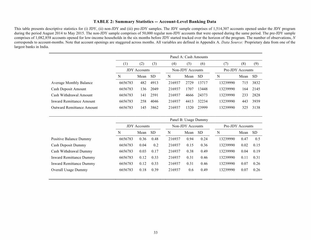
33

TABLE 2: Summary Statistics -- Account-Level Banking Data

This table presents descriptive statistics for (i) JDY, (ii) non-JDY and (iii) pre-JDY samples. The JDY sample comprises of 1,514,307 accounts opened under the JDY program during the period August 2014 to May 2015. The non-JDY sample comprises of 50,000 regular non-JDY accounts that were opened during the same period. The pre-JDY sample comprises of 1,082,858 accounts opened for low-income households in the six months before JDY started tracked over the horizon of the program. The number of observations, N corresponds to account-months. Note that account openings are staggered across months. All variables are defined in Appendix A. Data Source: Proprietary data from one of the largest banks in India.

Panel A: Cash Amounts

(1) (2) (3) (4) (5) (6) (7) (8) (9)

JDY Accounts Non-JDY Accounts Pre-JDY Accounts N Mean SD N Mean SD N Mean SD

Average Monthly Balance 6656783 482 4913 216937 2729 13717 13239990 715 3832 Cash Deposit Amount 6656783 136 2049 216937 1707 13448 13239990 164 2145 Cash Withdrawal Amount 6656783 141 2591 216937 4666 24373 13239990 233 2828 Inward Remittance Amount 6656783 258 4046 216937 4413 32234 13239990 443 3939 Outward Remittance Amount 6656783 145 3862 216937 1320 23999 13239990 325 3138 Panel B: Usage Dummy JDY Accounts Non-JDY Accounts Pre-JDY Accounts

N Mean SD N Mean SD N Mean SD

Positive Balance Dummy 6656783 0.36 0.48 216937 0.94 0.24 13239990 0.47 0.5 Cash Deposit Dummy 6656783 0.04 0.2 216937 0.15 0.36 13239990 0.02 0.15 Cash Withdrawal Dummy 6656783 0.03 0.17 216937 0.38 0.49 13239990 0.04 0.19 Inward Remittance Dummy 6656783 0.12 0.33 216937 0.31 0.46 13239990 0.11 0.31 Inward Remittance Dummy 6656783 0.12 0.33 216937 0.31 0.46 13239990 0.07 0.26 Overall Usage Dummy 6656783 0.18 0.39 216937 0.6 0.49 13239990 0.07 0.26

34

TABLE 3: Panel A – JDY Account Level Analysis of Average Balance and Usage Relative to Non-JDY

Accounts

This table reports the coefficient estimates from the following regression model: Balanceit = β0 + β1 J DYit + β2 Ageit + β3 J DY × Age + Xi,t + Account Opening Datet + εit Where i refers to unique bank account, and t refers to year-month. Balance is Average monthly balance in column (1), a dummy variable that takes the value 1 for accounts-months with positive balance in columns (2) and a dummy variable that takes the value 1 for accounts-months if at least one transaction was performed by the account holder in column (3). Age is the number of months since account opening. JDY is a dummy variable that identifies accounts opened under the JDY program. In these baseline tests, we focus on the periods up to 10 months after the commencement of Jan Dhan Yojna (JDY) (August (2014) to May (2015)). The excluded category is non-JDY accounts as defined in Section III. All variables are defined in detail in Appendix A. Proprietary data was obtained from one of the largest banks in India. Account-clustered robust standard errors are reported in parentheses. *, **, and *** indicate significance at 10%, 5%, and 1% levels respectively.

Average Monthly Balance

Positive Balance Dummy

Positive Usage Dummy

(1) (2) (3)

JDY -2370.967*** -0.724*** -0.441***

(91.073) (0.002) (0.002)

Age of Account 46.776** 0.005*** -0.008***

(18.858) (0.000) (0.001) Age of Account X JDY 57.791*** 0.044*** 0.011*** (18.773) (0.000) (0.001)

N 6698136 6698136 6698136

R2 0.007 0.079 0.046

35

TABLE 3: Panel B – JDY Account Level Analysis of Cash Deposits and Withdrawals Relative to Non-JDY Accounts

This table reports the coefficient estimates from the following regression model: Transactionit = β0 + β1 J DYit + β2 Ageit + β3 J DY × Age + Xi,t + Account Opening Datet + εit Where i refers to unique bank account, and t refers to year-month. Transaction in panel B is one of the 12 variables defined in Appendix A based on deposit and withdrawal transactions. Age is the number of months since account opening. JDY is a dummy variable that identifies accounts opened under the JDY program. In these baseline tests, we focus on the periods up to 10 months after the commencement of Jan Dhan Yojna (JDY) (August 2014 to May 2015). The excluded category is non-JDY accounts as defined in Section III. Proprietary data was obtained from one of the largest banks in India. Account-clustered robust standard errors are reported in parentheses. *, **, and *** indicate significance at 10%, 5%, and 1% levels respectively.

Cash Deposit # Cash Deposit Cash Deposit

Cash Withdrawal

# Cash Withdrawal Cash Withdrawal

Amount Transactions Dummy Amount Transactions Dummy

(1) (2) (3) (4) (5) (6)

JDY -1667.757*** -0.186*** -0.115*** -4819.868*** -1.214*** -0.375*** (72.667) (0.004) (0.002) (135.149) (0.015) (0.003)

Age of Account -32.856** -0.013*** -0.010*** -77.230*** -0.005* -0.005*** (14.295) (0.001) 0.000 (29.457) (0.003) (0.001) Age of Account X JDY 38.371*** 0.008*** 0.005*** 103.159*** 0.018*** 0.012*** (14.411) (0.001) 0.000 (29.452) (0.003) (0.001) N 6698136 6698136 6698136 6698136 6698136 6698136 R2 0.008 0.016 0.015 0.025 0.097 0.109

36

TABLE 3: Panel C - JDY Account Level Analysis of Inward and Outward Remittances Relative to Non-JDY Accounts

This table reports the coefficient estimates from the following regression model: Transactionit = β0 + β1 J DYit + β2 Ageit + β3 J DY × Age + Xi,t + Account Opening Datet + εit Where i refers to unique bank account, and t refers to year-month. Transaction in Panel C is one of the 12 variables defined in appendix A based on remittance transactions. Age is the number of months since account opening. JDY is a dummy variable that identifies accounts opened under the JDY program. In these baseline tests, we focus on the periods up to 10 months after the commencement of Jan Dhan Yojna (JDY) (August 2014 to May 2015). The excluded category is non-JDY accounts as defined in Section III. Proprietary data was obtained from one of the largest banks in India. Account-clustered robust standard errors are reported in parentheses. *, **, and *** indicate significance at 10%, 5%, and 1% levels respectively.

Inward Remittance

# Inward Remittance

Inward Remittance

Outward Remittance

# Outward Remittance

Outward Remittance

Amount Transactions Dummy Amount Transactions Dummy

(1) (2) (3) (4) (5) (6)

JDY -4193.301*** -0.335*** -0.186*** -1238.127*** -0.329*** -0.194*** (166.631) (0.033) (0.002) (140.342) (0.010) (0.002) Age of Account -18.304 0.003 0.004*** -10.922 0.023*** 0.004*** (39.136) (0.002) (0.001) (28.713) (0.002) (0.000) Age of Account X JDY 22.173 0.00 -0.001 17.852 -0.021*** -0.003*** (39.038) (0.002) (0.001) (28.535) (0.002) (0.000) N 6698136 6698136 6698136 6698136 6698136 6698136 R2 0.011 0.003 0.028 0.001 0.01 0.037

37

Table 4: Regional Summary Statistics

This table presents summary statistics for the districts in our sample. Panels A and B report the statistics based on the exposure measures, Adults per Unit Bank Branch which is the ratio of total adult population to the total number of bank branches in a district and %age State-Owned Bank Branches in a district which is the ratio of total number of bank branches that are owned by state-owned banks to the total number of bank branches in each district. Higher values for both these measures imply greater ex-ante JDY exposure. We split our sample into two based on these measures. Columns (1) and (2) (columns (3) and (4)) report statistics for the districts with above (below) median value of Adults per Unit Bank Branch (Panel A) and % State-Owned Bank Branches (Panel B). All variables are defined in Appendix A.

Panel A: Exposure Measure - Adults per Unit Bank Branch

(1) (2) (3) (4)

Above Median Below Median

Mean SD Mean SD

Total Region GDP Per Capita in INR Per Capita 50051 25849 195000 1530000

All Industry GDP Per Capita in INR Per Capita 12511 11207 40171 138000

Agriculture GDP Per Capita in INR Per Capita 7717 8769 9316 9046

Agriculture and Related Per Capita in INR Per Capita 13187 10479 15815 13869

Manufacturing GDP Per Capita in INR Per Capita 3584 5014 19823 72157

Banking GDP Per Capita in INR Per Capita 4387 2470 62272 753000

Adults Per unit Bank Branch 9461 2976 4390 1335

Panel B: Exposure Measure - % State-Owned Bank Branches

Above Median Below Median

Mean SD Mean SD

Total Region GDP in INR Per Capita 55414 33480 190000 1530000

All Industry GDP in INR Per Capita 14704 16674 37867 137000

Agriculture GDP in INR Per Capita 7870 9187 9157 8642

Agriculture and Related in INR Per Capita 13752 11152 15236 13408

Manufacturing GDP in INR Per Capita 3999 6668 19351 72003

Banking GDP in INR Per Capita 4975 3687 61490 751000

% State-Owned Branches 94 3 79 13

38

Table 4: Regional Summary Statistics [continued]

This table presents summary statistics for the districts in our sample. Panels C and D report the statistics based on the exposure measures, % Households Without Bank Accounts, which is the ratio of total number of households without any bank account, to the total number of households in a district and Financial Inclusion Index which is a comprehensive measure of financial inclusion released by CRISIL which combines three critical parameters of basic financial services: branch penetration, deposit penetration, and credit penetration into one single metric in the form of an index. It is a relative index that has a scale of 0 to 100 with higher number indicating lower levels of financial inclusion. Higher values for both these measures imply greater ex-ante JDY exposure. We split our sample into two based on these measures. Columns (1) and (2) (columns (3) and (4)) report statistics for the districts with above (below) median value of % Households Without Bank Accounts (Panel C) and Financial Inclusion Index (Panel D). All variables are defined in Appendix A.

Panel C: Exposure Measure - % Households Without Bank Accounts

(1) (2) (3) (4)

Above Median Below Median

Mean SD Mean SD

Total Region GDP in INR Per Capita 60282 29472 185000 1530000

All Industry GDP in INR Per Capita 16015 12469 36544 138000

Agriculture GDP in INR Per Capita 8971 9558 8045 8250

Agriculture and Related in INR Per Capita 14754 11645 14224 13015

Manufacturing GDP in INR Per Capita 5528 7169 17808 72251

Banking GDP in INR Per Capita 6379 6679 60073 751000

% Households Without Bank Accounts 56 10 28 9

Panel D: Exposure Measure - Financial Inclusion Index

(1) (2) (3) (4)

Above Median Below Median

Mean SD Mean SD

Total Region GDP in INR Per Capita 54556 32558 189000 1520000

All Industry GDP in INR Per Capita 14541 16987 37806 137000

Agriculture GDP in INR Per Capita 7776 9115 9238 8709

Agriculture and Related in INR Per Capita 13803 11605 15171 13007

Manufacturing GDP in INR Per Capita 4013 7040 19190 71641

Banking GDP in INR Per Capita 4754 4332 61166 748000

Financial Inclusion Index 68 8 38 14

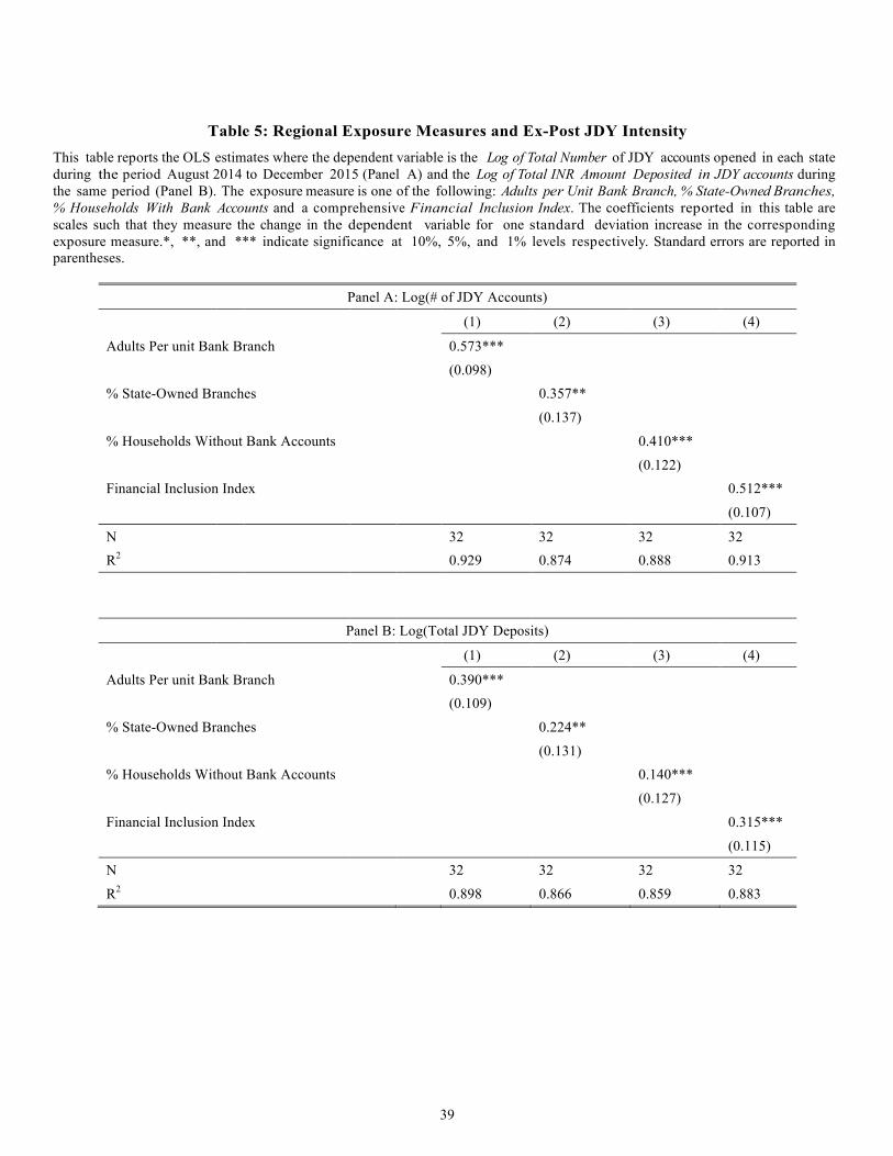
39

Table 5: Regional Exposure Measures and Ex-Post JDY Intensity

This table reports the OLS estimates where the dependent variable is the Log of Total Number of JDY accounts opened in each state during the period August 2014 to December 2015 (Panel A) and the Log of Total INR Amount Deposited in JDY accounts during the same period (Panel B). The exposure measure is one of the following: Adults per Unit Bank Branch, % State-Owned Branches, % Households With Bank Accounts and a comprehensive Financial Inclusion Index. The coefficients reported in this table are scales such that they measure the change in the dependent variable for one standard deviation increase in the corresponding exposure measure.*, **, and *** indicate significance at 10%, 5%, and 1% levels respectively. Standard errors are reported in parentheses.

Panel A: Log(# of JDY Accounts)

(1) (2) (3) (4)

Adults Per unit Bank Branch 0.573*** (0.098)

% State-Owned Branches 0.357** (0.137)

% Households Without Bank Accounts 0.410***

(0.122) Financial Inclusion Index 0.512***

(0.107)

N 32 32 32 32 R2 0.929 0.874 0.888 0.913

Panel B: Log(Total JDY Deposits)

(1) (2) (3) (4)

Adults Per unit Bank Branch 0.390*** (0.109)

% State-Owned Branches 0.224** (0.131)

% Households Without Bank Accounts 0.140***

(0.127) Financial Inclusion Index 0.315***

(0.115)

N 32 32 32 32

R2 0.898 0.866 0.859 0.883

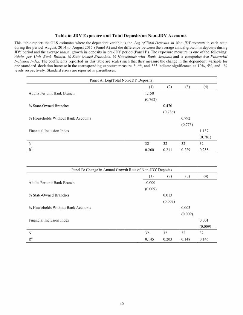
40

Table 6: JDY Exposure and Total Deposits on Non-JDY Accounts

This table reports the OLS estimates where the dependent variable is the Log of Total Deposits in Non-JDY accounts in each state during the period August, 2014 to August 2015 ( Panel A) and the difference between the average annual growth in deposits during JDY period and the average annual growth in deposits in pre-JDY period (Panel B). The exposure measure is one of the following: Adults per Unit Bank Branch, % State-Owned Branches, % Households with Bank Accounts and a comprehensive Financial Inclusion Index. The coefficients reported in this table are scales such that they measure the change in the dependent variable for one standard deviation increase in the corresponding exposure measure. *, **, and *** indicate significance at 10%, 5%, and 1% levels respectively. Standard errors are reported in parentheses.

Panel A: Log(Total Non-JDY Deposits)

(1) (2) (3) (4)

Adults Per unit Bank Branch 1.158 (0.762)

% State-Owned Branches 0.470 (0.786)

% Households Without Bank Accounts 0.792 (0.773)

Financial Inclusion Index 1.137 (0.781)

N 32 32 32 32 R2 0.260 0.211 0.229 0.255

Panel B: Change in Annual Growth Rate of Non-JDY Deposits

(1) (2) (3) (4)

Adults Per unit Bank Branch -0.000 (0.009)

% State-Owned Branches 0.013 (0.009)

% Households Without Bank Accounts 0.003 (0.009)

Financial Inclusion Index 0.001 (0.009)

N 32 32 32 32 R2 0.145 0.203 0.148 0.146

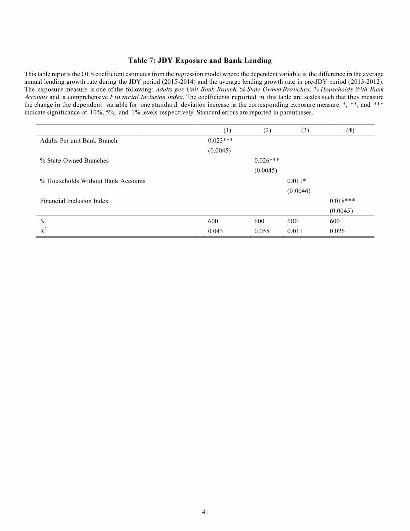
41

Table 7: JDY Exposure and Bank Lending

This table reports the OLS coefficient estimates from the regression model where the dependent variable is the difference in the average annual lending growth rate during the JDY period (2015-2014) and the average lending growth rate in pre-JDY period (2013-2012). The exposure measure is one of the following: Adults per Unit Bank Branch, % State-Owned Branches, % Households With Bank Accounts and a comprehensive Financial Inclusion Index. The coefficients reported in this table are scales such that they measure the change in the dependent variable for one standard deviation increase in the corresponding exposure measure. *, **, and *** indicate significance at 10%, 5%, and 1% levels respectively. Standard errors are reported in parentheses.

(1) (2) (3) (4) Adults Per unit Bank Branch 0.023***

(0.0045) % State-Owned Branches 0.026***

(0.0045) % Households Without Bank Accounts 0.011*

(0.0046) Financial Inclusion Index 0.018*** (0.0045) N 600 600 600 600 R2 0.043 0.055 0.011 0.026

42

TABLE 8: Regional Exposure Measure and Bank Loans (Bank Data)

This table reports the OLS coefficient estimates from the regression model where the dependent variable is the difference in the average monthly lending growth rate during the JDY period (2015-2014) and the average monthly lending growth rate in period before JDY (2013-2012). The exposure measure is one of the following: Adults per Unit Bank Branch, % State-Owned Branches, %age Households With Bank Accounts and a comprehensive Financial Inclusion Index. The coefficients reported in this table are scales such that they measure the change in the dependent variable for one standard deviation increase in the corresponding exposure measure. *, **, and *** indicate significance at 10%, 5%, and 1% levels respectively. Standard errors are reported in parentheses.

Monthly Growth in Total Loan Amount (1) (2) (3) (4) Adults Per unit Bank Branch 0.055***

(0.011) % State-Owned Branches 0.032***

(0.011) % Households Without Bank Accounts 0.031***

(0.011) Financial Inclusion Index 0.041*** (0.011) N 600 600 600 600 R2 0.039 0.013 0.012 0.022

43

TABLE 9: Regional Exposure Measure and Bank Loan Delinquency (Bank Data)This table reports the OLS coefficient estimates from the regression model where the dependent variable is the difference between the average default rate on newly originated loans during the JDY period minus the average monthly default rate (2014, September to 2015 September) on loans originated just prior to the JDYperiod (2014, January to 2014 July), where default rate is defined as the proportion of loans originated in a given month that become 60-day delinquent (panel A) or 90-day delinquent (panel B) within a year from loan origination. The exposure measure is one of the following: Adults per Unit Bank Branch, % State-Owned Branches, % Households With Bank Accounts and a comprehensive Financial Inclusion Index. The coefficients reported in this table are scales such that they measure the change in the dependent variable for one standard deviation increase in the corresponding exposure measure. *, **, and *** indicate significance at 10%, 5%, and 1% levels respectively. Standard errors are reported in parentheses.

Panel A: Default Rate – 60-day delinquency

(1) (2) (3) (4) Adults Per unit Bank Branch 0.004***

(0.001) % State-Owned Branches 0.001

(0.001) % Households Without Bank Accounts 0.004***

(0.001) Financial Inclusion Index 0.002* (0.001) N 439 439 439 438 R2 0.030 0.003 0.026 0.006

Panel B: Default Rate – 90-day delinquency

(1) (2) (3) (4)

Adults Per unit Bank Branch 0.003*** (0.001)

% State-Owned Branches 0.001 (0.001)

% Households Without Bank Accounts 0.003*** (0.001)

Financial Inclusion Index 0.002* (0.001)

N 439 439 439 438 R2 0.027 0.003 0.018 0.007

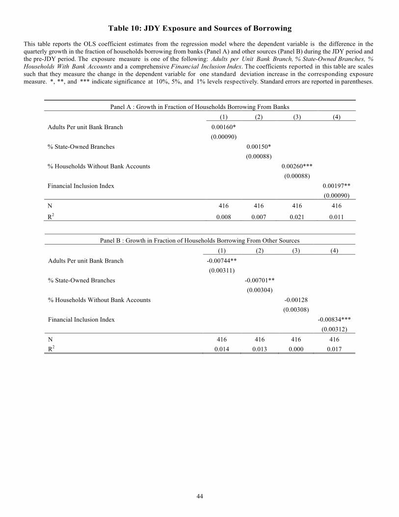
44

Table 10: JDY Exposure and Sources of Borrowing This table reports the OLS coefficient estimates from the regression model where the dependent variable is the difference in the quarterly growth in the fraction of households borrowing from banks (Panel A) and other sources (Panel B) during the JDY period and the pre-JDY period. The exposure measure is one of the following: Adults per Unit Bank Branch, % State-Owned Branches, % Households With Bank Accounts and a comprehensive Financial Inclusion Index. The coefficients reported in this table are scales such that they measure the change in the dependent variable for one standard deviation increase in the corresponding exposure measure. *, **, and *** indicate significance at 10%, 5%, and 1% levels respectively. Standard errors are reported in parentheses.

Panel A : Growth in Fraction of Households Borrowing From Banks (1) (2) (3) (4)

Adults Per unit Bank Branch 0.00160* (0.00090)

% State-Owned Branches 0.00150* (0.00088)

% Households Without Bank Accounts 0.00260*** (0.00088)

Financial Inclusion Index 0.00197** (0.00090)

N 416 416 416 416

R2 0.008 0.007 0.021 0.011

Panel B : Growth in Fraction of Households Borrowing From Other Sources (1) (2) (3) (4)

Adults Per unit Bank Branch -0.00744** (0.00311)

% State-Owned Branches -0.00701** (0.00304)

% Households Without Bank Accounts -0.00128 (0.00308)

Financial Inclusion Index -0.00834*** (0.00312)

N 416 416 416 416 R2 0.014 0.013 0.000 0.017

45

Table 11: JDY Exposure and Purpose of Borrowing This table reports the OLS coefficient estimates from the regression model where the dependent variable is the difference in the quarterly growth in the fraction of households borrowing from banks from households for consumption expenditure (Panel A) and medical expenditure (Panel B). during the JDY period and the pre-JDY period. The exposure measure is one of the following: Adults per Unit Bank Branch, %age State-Owned Branches, %age Households With Bank Accounts and a comprehensive Financial Inclusion Index. The coefficients reported in this table are scales such that they measure the change in the dependent variable for one standard deviation increase in the corresponding exposure measure.. *, **, and *** indicate significance at 10%, 5%, and 1% levels respectively. Standard errors are reported in parentheses.

Panel A: Growth in Fraction of Households Borrowing from Bank for Consumption Expenditure

(1) (2) (3) (4)

Adults Per unit Bank Branch -0.00020

(0.00022)

% State-Owned Branches -0.00018

(0.00022)

% Households Without Bank Accounts -0.00018

(0.00022)

Financial Inclusion Index -0.00040*

(0.00022)

N 416 416 416 416

R2 0.002 0.002 0.002 0.008

Panel B : Growth in Fraction of Households Borrowing from Bank for Medical Expenditure (1) (2) (3) (4)

Adults Per unit Bank Branch 0.00039*** (0.00011)

% State-Owned Branches 0.00012 (0.00011)

% Households Without Bank Accounts 0.00023** (0.00011)

Financial Inclusion Index 0.00018* (0.00011)

N 416 416 416 416 R2 0.031 0.003 0.012 0.007

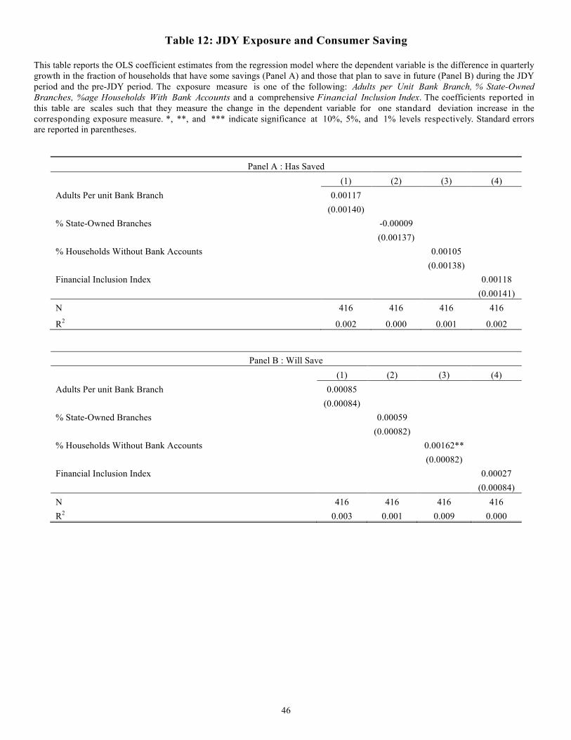
46

Table 12: JDY Exposure and Consumer Saving This table reports the OLS coefficient estimates from the regression model where the dependent variable is the difference in quarterly growth in the fraction of households that have some savings (Panel A) and those that plan to save in future (Panel B) during the JDY period and the pre-JDY period. The exposure measure is one of the following: Adults per Unit Bank Branch, % State-Owned Branches, %age Households With Bank Accounts and a comprehensive Financial Inclusion Index. The coefficients reported in this table are scales such that they measure the change in the dependent variable for one standard deviation increase in the corresponding exposure measure. *, **, and *** indicate significance at 10%, 5%, and 1% levels respectively. Standard errors are reported in parentheses.

Panel A : Has Saved (1) (2) (3) (4)

Adults Per unit Bank Branch 0.00117 (0.00140)

% State-Owned Branches -0.00009 (0.00137)

% Households Without Bank Accounts 0.00105 (0.00138)

Financial Inclusion Index 0.00118 (0.00141)

N 416 416 416 416

R2 0.002 0.000 0.001 0.002

Panel B : Will Save (1) (2) (3) (4)

Adults Per unit Bank Branch 0.00085 (0.00084)

% State-Owned Branches 0.00059 (0.00082)

% Households Without Bank Accounts 0.00162** (0.00082)

Financial Inclusion Index 0.00027 (0.00084)

N 416 416 416 416 R2 0.003 0.001 0.009 0.000

47

Table 13: JDY Exposure and Health Expenditure This table reports the OLS coefficient estimates from the regression model where the dependent variable is the difference in the monthly growth in household health expenditure during the JDY period and the pre-JDY period. The exposure measure is one of the following: Adults per Unit Bank Branch, % State-Owned Branches, %age Households With Bank Accounts and a comprehensive Financial Inclusion Index. The coefficients reported in this table are scales such that they measure the change in the dependent variable for one standard deviation increase in the corresponding exposure measure. *, **, and *** indicate significance at 10%, 5%, and 1% levels respectively. Standard errors are reported in parentheses.

Panel A : Expense on Health (1) (2) (3) (4)

Adults Per unit Bank Branch 0.034*** (0.007)

% State-Owned Branches 0.024*** (0.007)

% Households Without Bank Accounts 0.018*** (0.007)

Financial Inclusion Index 0.030*** (0.007)

N 419 419 419 419 R2 0.060 0.031 0.017 0.044

Panel B : Expense on Doctors and Physiotherapists Fee (1) (2) (3) (4)

Adults Per unit Bank Branch 0.015** (0.006)

% State-Owned Branches 0.006 (0.006)

% Households Without Bank Accounts -0.003 (0.006)

Financial Inclusion Index 0.021*** (0.006)

N 419 419 419 419 R2 0.015 0.002 0.001 0.030

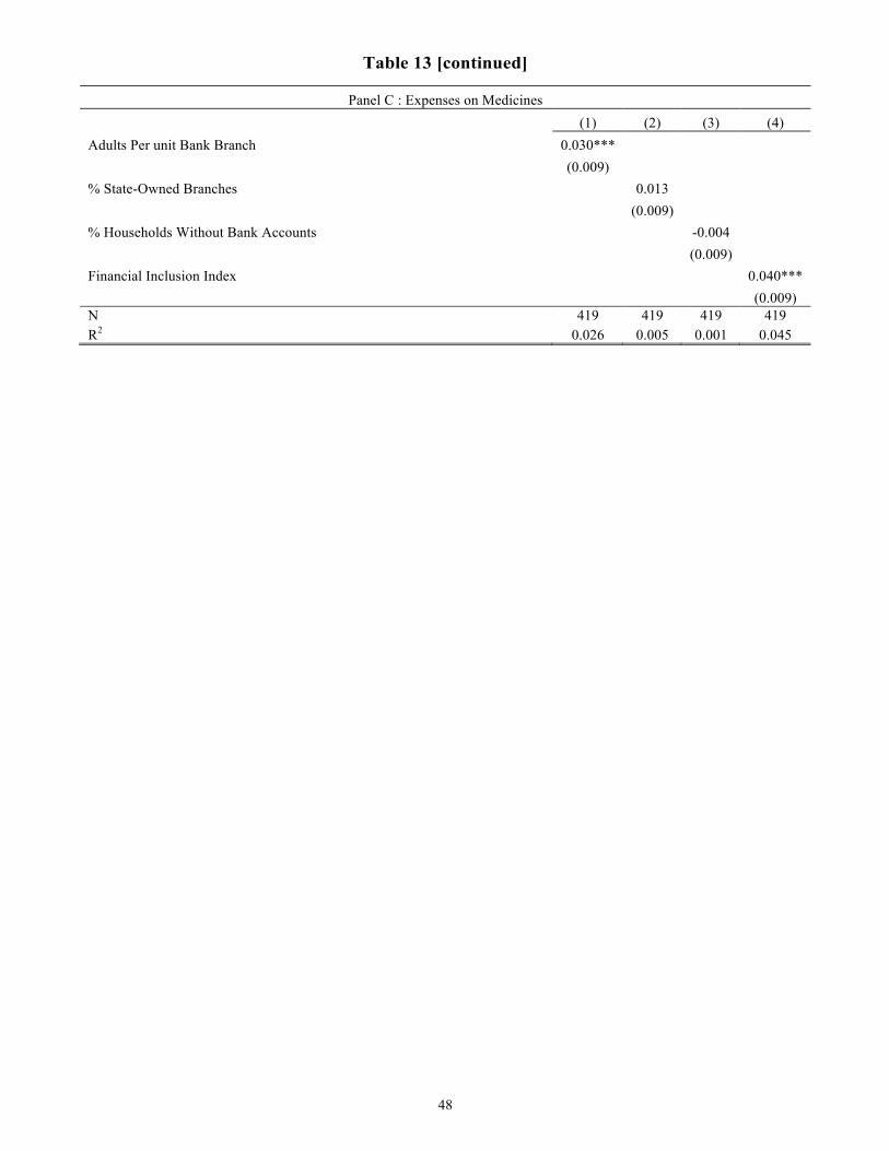
48

Table 13 [continued]

Panel C : Expenses on Medicines (1) (2) (3) (4)

Adults Per unit Bank Branch 0.030*** (0.009)

% State-Owned Branches 0.013 (0.009)

% Households Without Bank Accounts -0.004 (0.009)

Financial Inclusion Index 0.040*** (0.009)

N 419 419 419 419 R2 0.026 0.005 0.001 0.045

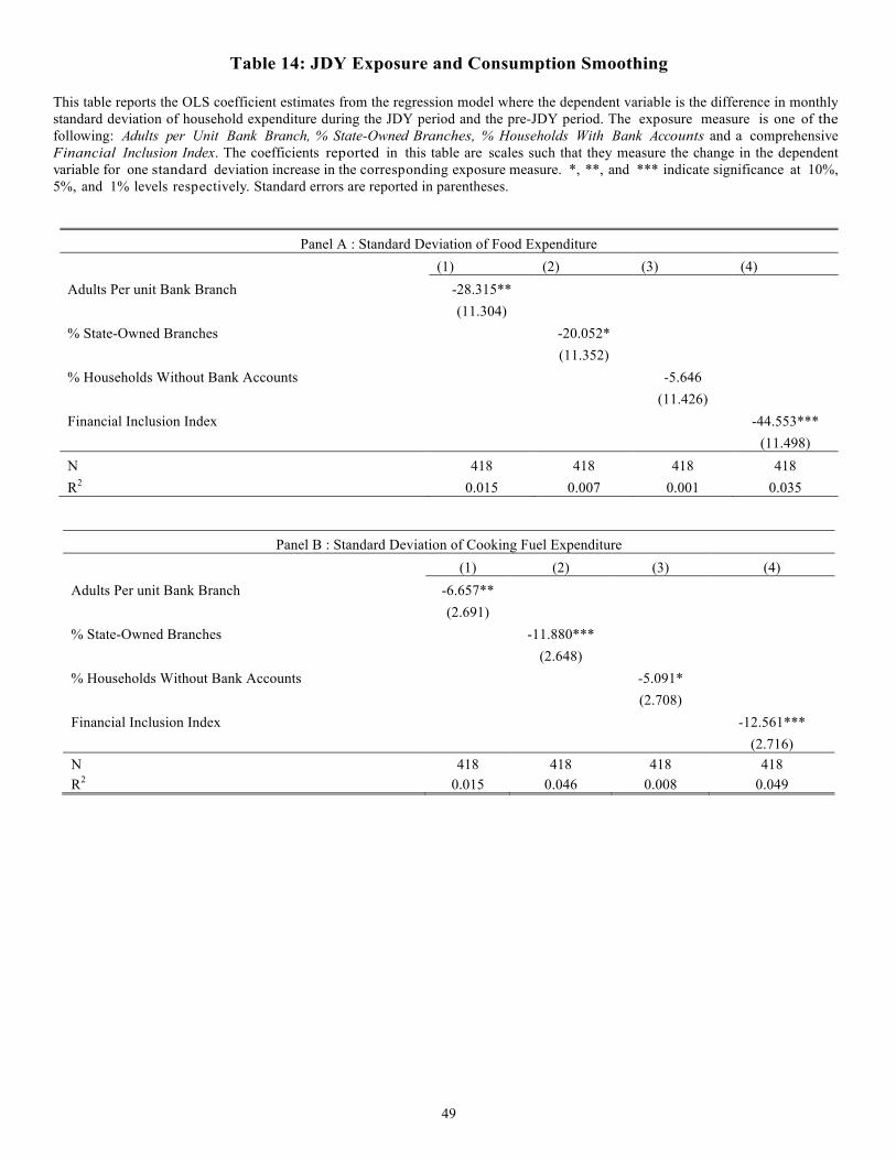
49

Table 14: JDY Exposure and Consumption Smoothing This table reports the OLS coefficient estimates from the regression model where the dependent variable is the difference in monthly standard deviation of household expenditure during the JDY period and the pre-JDY period. The exposure measure is one of the following: Adults per Unit Bank Branch, % State-Owned Branches, % Households With Bank Accounts and a comprehensive Financial Inclusion Index. The coefficients reported in this table are scales such that they measure the change in the dependent variable for one standard deviation increase in the corresponding exposure measure. *, **, and *** indicate significance at 10%, 5%, and 1% levels respectively. Standard errors are reported in parentheses.

Panel A : Standard Deviation of Food Expenditure (1) (2) (3) (4)

Adults Per unit Bank Branch -28.315** (11.304)

% State-Owned Branches -20.052* (11.352)

% Households Without Bank Accounts -5.646 (11.426)

Financial Inclusion Index -44.553*** (11.498)

N 418 418 418 418 R2 0.015 0.007 0.001 0.035

Panel B : Standard Deviation of Cooking Fuel Expenditure (1) (2) (3) (4)

Adults Per unit Bank Branch -6.657** (2.691)

% State-Owned Branches -11.880*** (2.648)

% Households Without Bank Accounts -5.091* (2.708)

Financial Inclusion Index -12.561*** (2.716)

N 418 418 418 418 R2 0.015 0.046 0.008 0.049

50

Figure 1: JDY Exposure and Deposit and Bank Lending Growth Rate

The figure shows the bank deposit percentage growth rates (panel (a)) and bank lending growth rates (panel (b)) in the more and less JDY exposed regions (based on the % of Households without Bank Accounts). The more exposed group is represented by the solid line, and the less exposed group is represented by the dashed line.

(a) Deposit Growth Rate (b) Lending Growth Rate

0%

5%

10%

15%

20%

25%

2012 2013 2014 2015

51

Figure 2: Synthetic Control: JDY Exposure and Bank Lending and Region GDP Growth Rates

The figure shows the bank lending growth rate (panel (a)) and GDP growth rates (panel (b)) in the more and less JDY exposed states (based on the % of Households without Bank Accounts). The more exposed group is represented by the solid line, and the less exposed synthetic control group is represented by the dashed line.

(a): Bank Lending Growth Rate (b): GDP Growth Rate

0%

2%

4%

6%

8%

10%

12%

14%

16%

18%

20%

2012 2013 2014 2015

52

Online Appendix A: Variable Definition

The Appendix describes some of the key variables used in our regional analysis.

• Accounts Per Capita: the ratio of total number of JDY accounts opened in each state during the period August, 2014 to December 2015, to the total number of adults in that state.

• Deposits Per Capita: the ratio of total amount Deposited in JDY accounts in each state during the period August, 2014 to December 2015, to the total number of adults in that state.

• Adults Per Unit Bank Branch: the ratio of the total adult population to the total number of bank branches in a state (or district).

• % State-Owned Bank Branches: the ratio of total number of bank branches that are owned by state-owned banks to the total number of bank branches in each state (district).

• % Households Without Bank Accounts: the ratio of total number of households without any bank account to the total number of households in each state (district).

• Financial Inclusion Index: a comprehensive district level measure of financial inclusion released by CRISIL, which combines three critical parameters of basic financial services: branch penetration, deposit penetration, and credit penetration into one single metric in the form of an index. It is a relative index that has a scale of 0 to 100 with higher numbers indicating lower levels of financial inclusion. For state level analysis, we use the average value of the index across all districts.

53

Online Appendix B: Additional Figures and Tests

The Appendix reports results of additional tests that are briefly described in the text. Additional details are available from the authors upon request.

54

Figure B1: Time Series of Aggregate Extensive Margin Statistics on JDY

The figure shows time series of aggregate statistics related to the JDY program: Number of Accounts Opened (Panels (a)), Number of Debit Cards issued (Panel (b)), Fraction of accounts with positive balance (panel (c)), and Total amount deposited in JDY accounts (panel (d)). The four lines represent the statistics respectively for JDY accounts opened by private banks, public (government owned) banks, regional rural banks and the total across all banks.

(a) Number Accounts Opened (b) Number Debit Cards Issued

(c) Number Accounts with Positive Balance (d) Total Deposits in JDY Accounts

55

Figure B2: Summary of Banking Transactions Performed The figure shows the distribution of number of one of four banking transactions: Cash Deposits (panels (a)), Cash Withdrawals (panel (b)), Inward Remittances (panel (c)), and Outward Remittances (panel (d)) during the first six months since an account opening.

(a) Cash Deposits (b) Cash Withdrawals

(c) Inward Remittances (d) Outward Remittances

81.1%

12.3%5.5% 0.9% 0.1% 0.0%

0%10%20%30%40%50%60%70%80%90%

100%

0 1 2 to 4 5 to 9 10 to 19 20+

87.3%

5.4% 4.4% 1.8% 0.8% 0.3%0%

10%20%30%40%50%60%70%80%90%

100%

0 1 2 to 4 5 to 9 10 to 19 20+

66.4%

16.9%11.9%

4.2% 0.4% 0.1%0%

10%20%30%40%50%60%70%80%90%

100%

0 1 2 to 4 5 to 9 10 to 19 20+

78.9%

14.7%4.8% 1.1% 0.3% 0.1%

0%10%20%30%40%50%60%70%80%90%

100%

0 1 2 to 4 5 to 9 10 to 19 20+

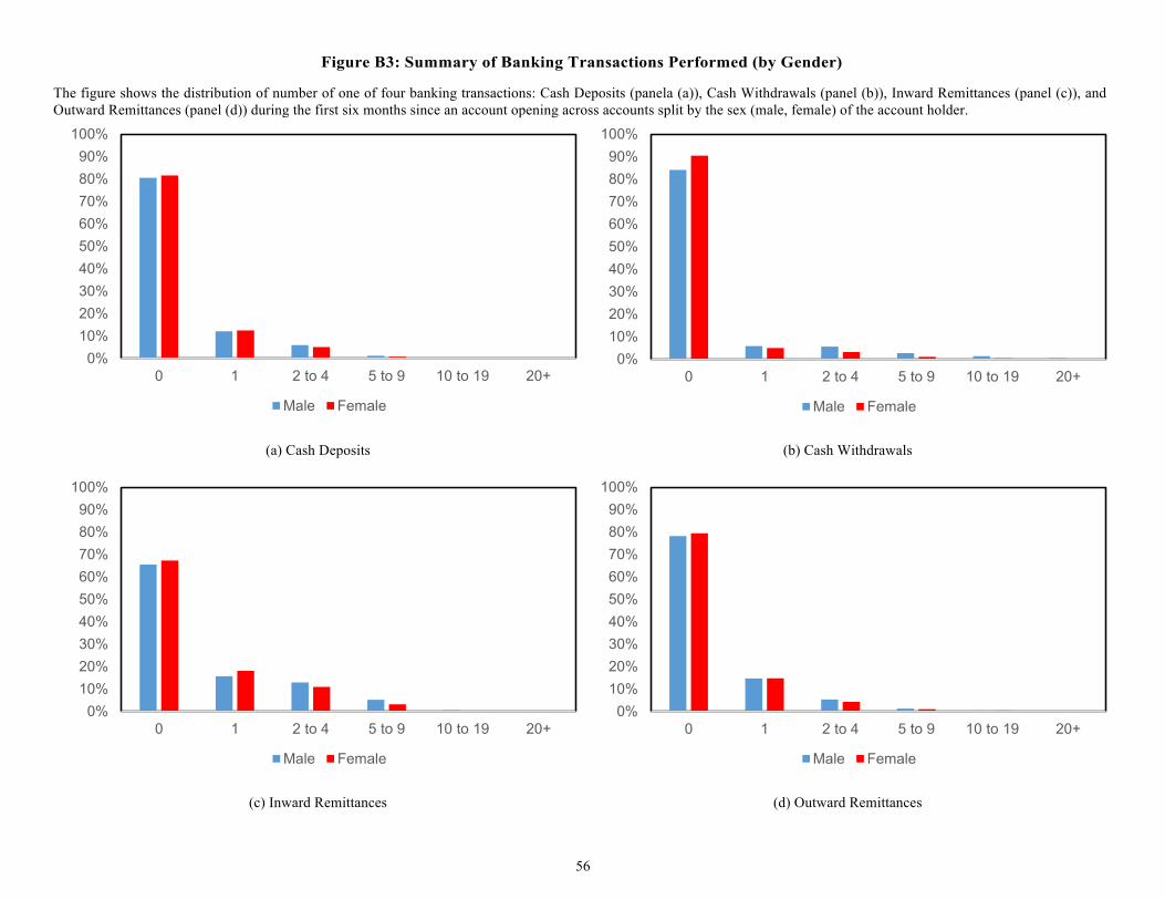
56

Figure B3: Summary of Banking Transactions Performed (by Gender)

The figure shows the distribution of number of one of four banking transactions: Cash Deposits (panela (a)), Cash Withdrawals (panel (b)), Inward Remittances (panel (c)), and Outward Remittances (panel (d)) during the first six months since an account opening across accounts split by the sex (male, female) of the account holder.

(a) Cash Deposits (b) Cash Withdrawals

(c) Inward Remittances (d) Outward Remittances

0%10%20%30%40%50%60%70%80%90%

100%

0 1 2 to 4 5 to 9 10 to 19 20+

Male Female

0%10%20%30%40%50%60%70%80%90%

100%

0 1 2 to 4 5 to 9 10 to 19 20+

Male Female

0%10%20%30%40%50%60%70%80%90%

100%

0 1 2 to 4 5 to 9 10 to 19 20+

Male Female

0%10%20%30%40%50%60%70%80%90%

100%

0 1 2 to 4 5 to 9 10 to 19 20+

Male Female

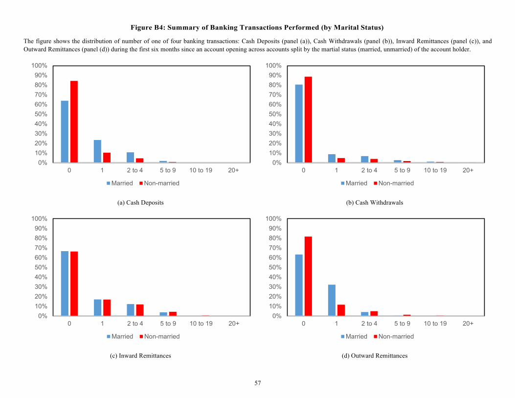
57

Figure B4: Summary of Banking Transactions Performed (by Marital Status)

The figure shows the distribution of number of one of four banking transactions: Cash Deposits (panel (a)), Cash Withdrawals (panel (b)), Inward Remittances (panel (c)), and Outward Remittances (panel (d)) during the first six months since an account opening across accounts split by the martial status (married, unmarried) of the account holder.

(a) Cash Deposits (b) Cash Withdrawals

(c) Inward Remittances (d) Outward Remittances

0%10%20%30%40%50%60%70%80%90%

100%

0 1 2 to 4 5 to 9 10 to 19 20+

Married Non-married

0%10%20%30%40%50%60%70%80%90%

100%

0 1 2 to 4 5 to 9 10 to 19 20+

Married Non-married

0%10%20%30%40%50%60%70%80%90%

100%

0 1 2 to 4 5 to 9 10 to 19 20+

Married Non-married

0%10%20%30%40%50%60%70%80%90%

100%

0 1 2 to 4 5 to 9 10 to 19 20+

Married Non-married

58

Figure B5: Summary of Banking Transactions Performed (by Age Quartiles) The figure shows the distribution of number of one of four banking transactions: Cash Deposits (panel (a)), Cash Withdrawals (panel (b)), Inward Remittances (panel (c)), and Outward Remittances (panel (d)) during the first six months since an account opening across accounts split by the age quartile of the account holder.

(a) Cash Deposits (b) Cash Withdrawals

(c) Inward Remittances (d) Outward Remittances

0%10%20%30%40%50%60%70%80%90%

100%

0 1 2 to 4 5 to 9 10 to 19 20+

Q1 Q2 Q3 Q4

0%10%20%30%40%50%60%70%80%90%

100%

0 1 2 to 4 5 to 9 10 to 19 20+

Q1 Q2 Q3 Q4

0%10%20%30%40%50%60%70%80%90%

100%

0 1 2 to 4 5 to 9 10 to 19 20+

Q1 Q2 Q3 Q4

0%10%20%30%40%50%60%70%80%90%

100%

0 1 2 to 4 5 to 9 10 to 19 20+

Q1 Q2 Q3 Q4

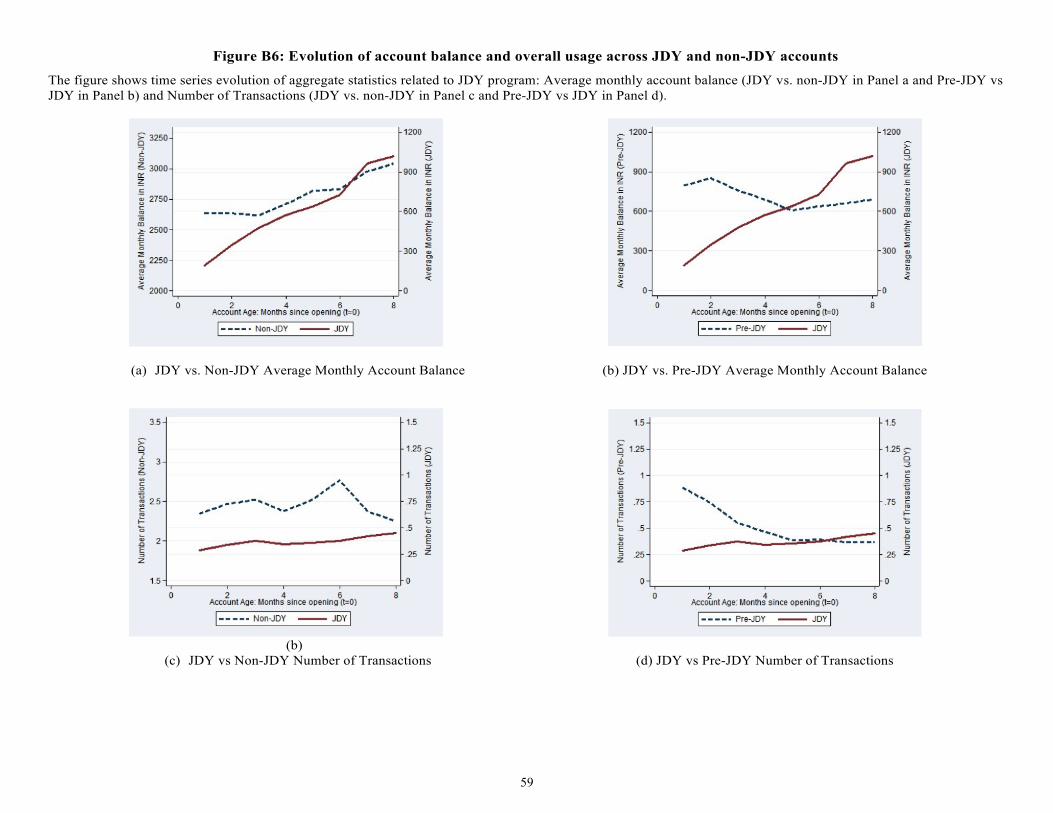
59

Figure B6: Evolution of account balance and overall usage across JDY and non-JDY accounts The figure shows time series evolution of aggregate statistics related to JDY program: Average monthly account balance (JDY vs. non-JDY in Panel a and Pre-JDY vs JDY in Panel b) and Number of Transactions (JDY vs. non-JDY in Panel c and Pre-JDY vs JDY in Panel d).

(a) JDY vs. Non-JDY Average Monthly Account Balance

(b) JDY vs. Pre-JDY Average Monthly Account Balance

(b)

(c) JDY vs Non-JDY Number of Transactions

(d) JDY vs Pre-JDY Number of Transactions

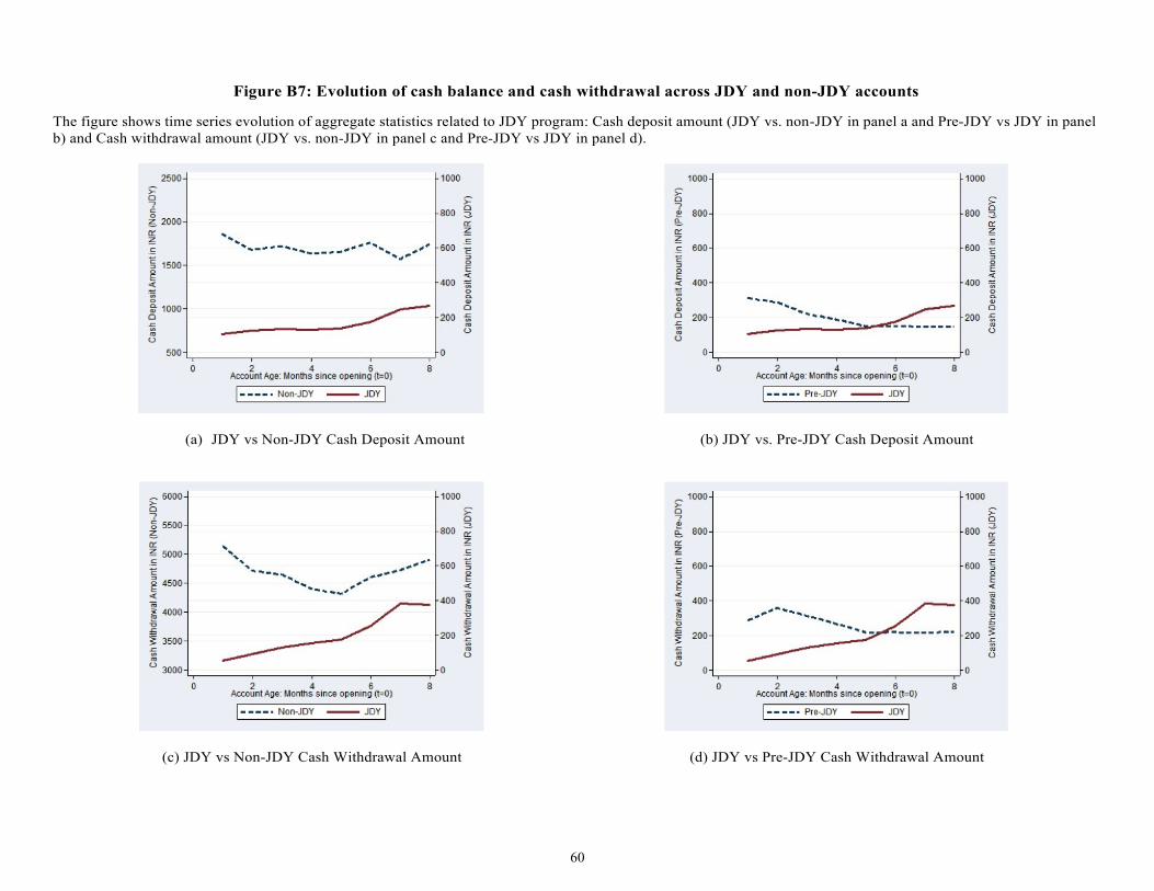
60

Figure B7: Evolution of cash balance and cash withdrawal across JDY and non-JDY accounts

The figure shows time series evolution of aggregate statistics related to JDY program: Cash deposit amount (JDY vs. non-JDY in panel a and Pre-JDY vs JDY in panel b) and Cash withdrawal amount (JDY vs. non-JDY in panel c and Pre-JDY vs JDY in panel d).

(a) JDY vs Non-JDY Cash Deposit Amount

(b) JDY vs. Pre-JDY Cash Deposit Amount

(c) JDY vs Non-JDY Cash Withdrawal Amount

(d) JDY vs Pre-JDY Cash Withdrawal Amount

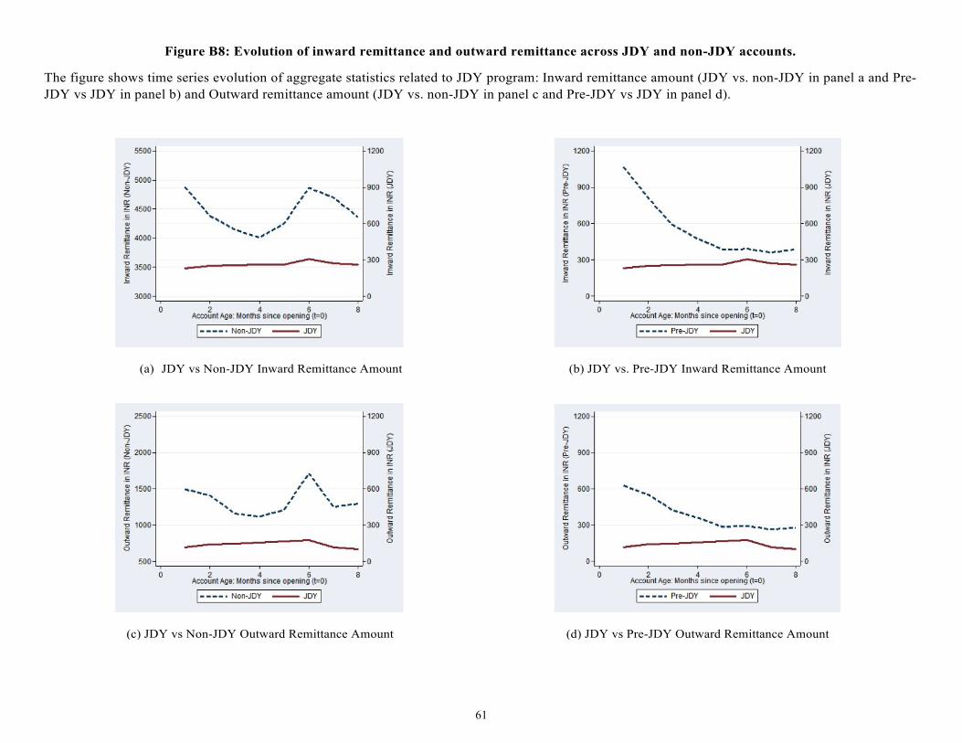
61

Figure B8: Evolution of inward remittance and outward remittance across JDY and non-JDY accounts.

The figure shows time series evolution of aggregate statistics related to JDY program: Inward remittance amount (JDY vs. non-JDY in panel a and Pre-JDY vs JDY in panel b) and Outward remittance amount (JDY vs. non-JDY in panel c and Pre-JDY vs JDY in panel d).

(a) JDY vs Non-JDY Inward Remittance Amount

(b) JDY vs. Pre-JDY Inward Remittance Amount

(c) JDY vs Non-JDY Outward Remittance Amount

(d) JDY vs Pre-JDY Outward Remittance Amount

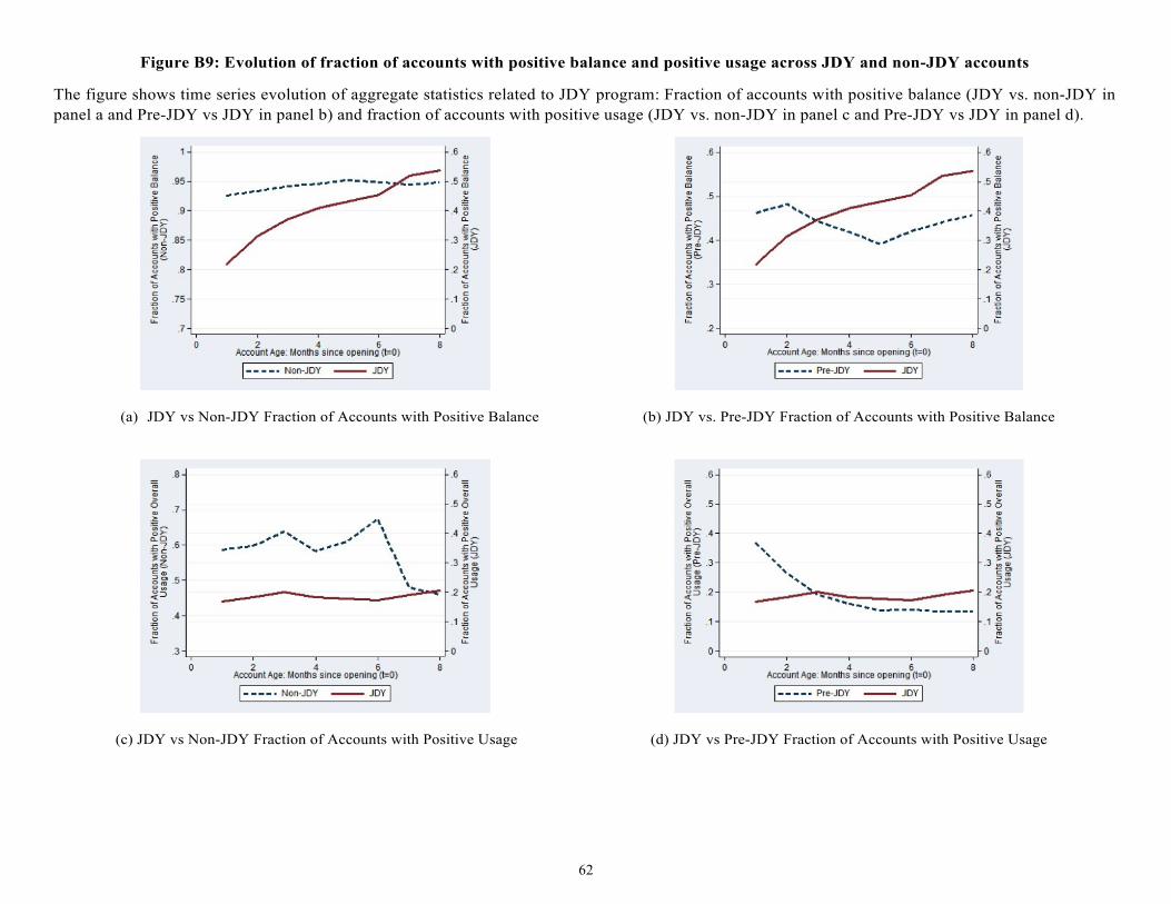
62

Figure B9: Evolution of fraction of accounts with positive balance and positive usage across JDY and non-JDY accounts

The figure shows time series evolution of aggregate statistics related to JDY program: Fraction of accounts with positive balance (JDY vs. non-JDY in panel a and Pre-JDY vs JDY in panel b) and fraction of accounts with positive usage (JDY vs. non-JDY in panel c and Pre-JDY vs JDY in panel d).

(a) JDY vs Non-JDY Fraction of Accounts with Positive Balance

(b) JDY vs. Pre-JDY Fraction of Accounts with Positive Balance

(c) JDY vs Non-JDY Fraction of Accounts with Positive Usage

(d) JDY vs Pre-JDY Fraction of Accounts with Positive Usage

63

Figure B10: Heterogeneity by Gender

The figure shows time series of aggregate statistics related to JDY program: Average monthly balance (JDY in panel a, Non-JDY in panel b and Pre-JDY in panel c) and Fraction of accounts with positive overall usage (JDY in panel d, Non-JDY in panel e and Pre-JDY in panel f).

(a) JDY Average Monthy Balance (b) Non-JDY Average Monthly Balance (c) Pre-JDY Average Monthly Balance

(d) JDY Fraction of Accounts with Positive Usage (e) Non-JDY Fraction of Accounts with Positive Usage (f) Pre-JDY Fraction of Accounts with Positive Usage

64

Figure B11: Heterogeneity by Age of Depositor

The figure shows time series of aggregate statistics related to JDY program: Average monthly balance (JDY in Panel a, Non-JDY in Panel b and Pre-JDY in Panel c) and Fraction of accounts with positive overall usage (JDY in Panel d, Non-JDY in Panel e and Pre-JDY in Panel f).

(a) JDY Average Monthy Balance (b) Non-JDY Average Monthly Balance (c) Pre-JDY Average Monthly Balance

(d) JDY Fraction of Accounts with Positive Usage (e) Non-JDY Fraction of Accounts with Positive Usage (f) Pre-JDY Fraction of Accounts with Positive Usage

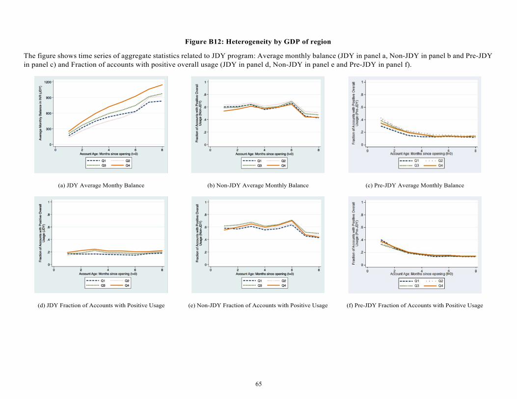
65

Figure B12: Heterogeneity by GDP of region

The figure shows time series of aggregate statistics related to JDY program: Average monthly balance (JDY in panel a, Non-JDY in panel b and Pre-JDY in panel c) and Fraction of accounts with positive overall usage (JDY in panel d, Non-JDY in panel e and Pre-JDY in panel f).

(a) JDY Average Monthy Balance (b) Non-JDY Average Monthly Balance (c) Pre-JDY Average Monthly Balance

(d) JDY Fraction of Accounts with Positive Usage (e) Non-JDY Fraction of Accounts with Positive Usage (f) Pre-JDY Fraction of Accounts with Positive Usage

66

Figure B13: Heterogeneity by Literacy of the Region

The figure shows time series of aggregate statistics related to JDY program: Average monthly balance (JDY in panel a, Non-JDY in panel b and Pre-JDY in panel c) and Fraction of accounts with positive overall usage (JDY in panel d, Non-JDY in panel e and Pre-JDY in panel f).

(a) JDY Average Monthy Balance (b) Non-JDY Average Monthly Balance (c) Pre-JDY Average Monthly Balance

(d) JDY Fraction of Accounts with Positive Usage (e) Non-JDY Fraction of Accounts with Positive Usage (f) Pre-JDY Fraction of Accounts with Positive Usage

67

TABLE B1: Panel A – JDY Account Level Analysis of Average Balance and Usage Relative to Pre-JDY Accounts

This table reports the coefficient estimates from the following regression model:

Balanceit = β0 + β1 J DYit + β2 Ageit + β3 J DY × Age + Xi,t + Account Opening Datet + εit

where i refers to unique bank account, and t refers to year-month. Balance is Average monthly balance in column (1), a dummy variable that takes the value 1 for accounts-months with positive balance in columns (2) and a dummy variable that takes the value 1 for accounts-months if at least one transaction was performed by the account holder in column (3). Age is the number of months since account opening. JDY is a dummy variable that identifies accounts opened under the JDY program. In these baseline tests, we focus on the periods up to 10 months after the commencement of Jan Dhan Yojna (JDY) (August (2014) to May (2015)). The excluded category is pre-JDY accounts as defined in Section III. All variables are defined in detail in appendix A. Proprietary data was obtained from one of the largest banks in India. Account-clustered robust standard errors are reported in parentheses. *, **, and *** indicate significance at 10%, 5%, and 1% levels respectively.

Average Monthly Balance Positive Balance Dummy Positive Usage Dummy

(1) (2) (3)

JDY -605.458*** -0.191*** -0.049*** (7.034) (0.001) (0.001) Age of Account 2.637*** 0.010*** -0.007***

(0.438) (0.000) (0.000) Age of Account X JDY 109.205*** 0.036*** 0.008***

(1.657) (0.000) (0.000)

N 19024045 19024045 19024045

R2 0.002 0.026 0.013

68

TABLE B1: Panel B – JDY Account Level Analysis of Cash Deposits and Withdrawals Relative to Pre-JDY Accounts

This table reports the coefficient estimates from the following regression model:

Transactionit = β0 + β1 J DYit + β2 Ageit + β3 J DY × Age + Xi,t + Account Opening Datet + εit

where i refers to unique bank account, and t refers to year-month. Transaction in panel B is one of the 12 variables defined in appendix A based on deposit and withdrawal transactions. Age is the number of months since account opening. JDY is a dummy variable that identifies accounts opened under the JDY program. In these baseline tests, we focus on the periods up to 10 months after the commencement of Jan Dhan Yojna (JDY) (August 2014 to May 2015). The excluded category is pre-JDY accounts as defined in Section III. Proprietary data was obtained from one of the largest banks in India. Account-clustered robust standard errors are reported in parentheses. *, **, and *** indicate significance at 10%, 5%, and 1% levels respectively.

Cash Deposit Amount

# Cash Deposit Transactions

Cash Deposit Dummy

Cash Withdrawal Amount

# Cash Withdrawal Transactions

Cash Withdrawal Dummy

(1) (2) (3) (4) (5) (6)

JDY -144.723*** 0.004*** 0.013*** -291.462*** -0.147*** -0.050*** (3.034) (0.000) (0.000) (3.689) (0.001) (0.000) Age of Account -8.641*** -0.002*** -0.002*** -8.118*** -0.005*** -0.002*** (0.201) (0.000) (0.000) (0.270) (0.000) (0.000) Age of Account X JDY 23.231*** 0.001*** -0.001*** 47.036*** 0.024*** 0.010*** (0.635) (0.000) (0.000) (0.726) (0.000) (0.000)

N 19024045 19024045 19024045 19024045 19024045 19024045 R2 0.001 0.003 0.006 0.002 0.009 0.014

69

TABLE B1: Panel C - JDY Account Level Analysis of Inward and Outward Remittances Relative to Pre-JDY Accounts

This table reports the coefficient estimates from the following regression model:

Transactionit = β0 + β1 J DYit + β2 Ageit + β3 J DY × Age + Xi,t + Account Opening Datet + εit

where i refers to unique bank account, and t refers to year-month. Transaction in panel C is one of the 12 variables defined in appendix A based on remittance transactions. Age is the number of months since account opening. JDY is a dummy variable that identifies accounts opened under the JDY program. In these baseline tests, we focus on the periods up to 10 months after the commencement of Jan Dhan Yojna (JDY) (August 2014 to May 2015). The excluded category is pre-JDY accounts as defined in Section III. Proprietary data was obtained from one of the largest banks in India. Account-clustered robust standard errors are reported in parentheses. *, **, and *** indicate significance at 10%, 5%, and 1% levels respectively.

Inward Remittance Amount

# Inward Remittance Transactions

Inward Remittance Dummy

Outward Remittance Amount

# Outward Remittance Transactions

Outward Remittance Dummy

(1) (2) (3) (4) (5) (6)

JDY -449.872*** -0.068*** -0.028*** -331.536*** -0.123*** -0.060*** (6.043) (0.001) (0.000) (5.594) (0.001) (0.000) Age of Account -27.364*** -0.008*** -0.005*** -14.832*** -0.006*** -0.002*** (0.396) (0.000) (0.000) (0.331) (0.000) (0.000) Age of Account X JDY 35.593*** 0.005*** 0.003*** 22.165*** 0.008*** 0.004*** (1.065) (0.000) (0.000) (1.051) (0.000) (0.000)

N 19024045 19024045 19024045 19024045 19024045 19024045 R2 0.001 0.004 0.014 0.001 0.002 0.009

70

Table B2: JDY Exposure and Health Outcomes

This table reports the OLS coefficient estimates from the regression model where the dependent variable is the difference in the average annual percentage change in health outcomes during the JDY period (2015-2014) and the annual percentage change in health outcomes in pre-JDY period (2013-2012). The exposure measure is one of the following: Adults per Unit Bank Branch, % State-Owned Branches, % Households With Bank Accounts and a comprehensive Financial Inclusion Index. The coefficients reported in this table are scales such that they measure the change in the dependent variable for one standard deviation increase in the corresponding exposure measure.*, **, and *** indicate significance at 10%, 5%, and 1% levels respectively. Standard errors are reported in parentheses.

Panel A: Death rate

(1) (2) (3) (4) Adults Per unit Bank Branch -0.019***

(0.005) % State-Owned Branches -0.004

(0.007) % Households Without Bank Accounts -0.017***

(0.006) Financial Inclusion Index -0.011* (0.006)

N 20 20 20 20 R2 0.408 0.020 0.329 0.146

Panel B: Death rate of common diseases

(1) (2) (3) (4) Adults Per unit Bank Branch -0.014

(0.097) % State-Owned Branches -0.090

(0.095) % Households Without Bank Accounts -0.020

(0.097) Financial Inclusion Index -0.001 (0.096) N 20 20 20 20 R2 0.001 0.037 0.002 0.000

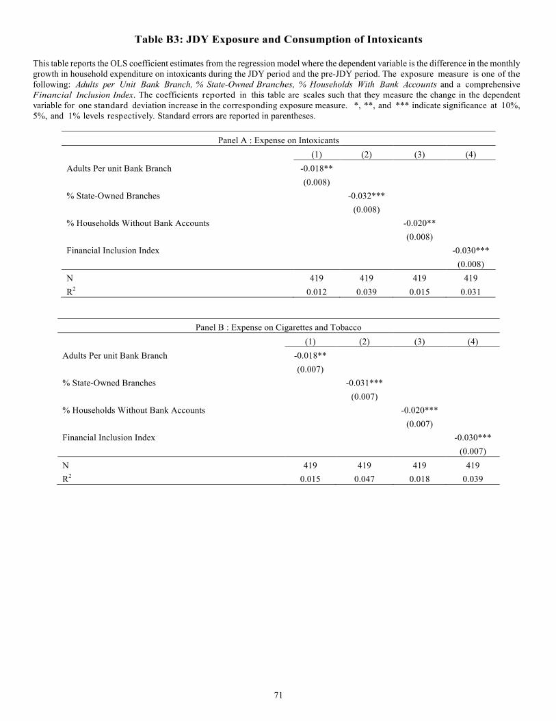
71

Table B3: JDY Exposure and Consumption of Intoxicants This table reports the OLS coefficient estimates from the regression model where the dependent variable is the difference in the monthly growth in household expenditure on intoxicants during the JDY period and the pre-JDY period. The exposure measure is one of the following: Adults per Unit Bank Branch, % State-Owned Branches, % Households With Bank Accounts and a comprehensive Financial Inclusion Index. The coefficients reported in this table are scales such that they measure the change in the dependent variable for one standard deviation increase in the corresponding exposure measure. *, **, and *** indicate significance at 10%, 5%, and 1% levels respectively. Standard errors are reported in parentheses.

Panel A : Expense on Intoxicants (1) (2) (3) (4)

Adults Per unit Bank Branch -0.018** (0.008)

% State-Owned Branches -0.032*** (0.008)

% Households Without Bank Accounts -0.020** (0.008)

Financial Inclusion Index -0.030*** (0.008)

N 419 419 419 419 R2 0.012 0.039 0.015 0.031

Panel B : Expense on Cigarettes and Tobacco (1) (2) (3) (4)

Adults Per unit Bank Branch -0.018** (0.007)

% State-Owned Branches -0.031*** (0.007)

% Households Without Bank Accounts -0.020*** (0.007)

Financial Inclusion Index -0.030*** (0.007)

N 419 419 419 419 R2 0.015 0.047 0.018 0.039

72

Table B3 [continued]

(1) (2) (3) (4)

Adults Per unit Bank Branch -0.018* (0.011)

% State-Owned Branches -0.019* (0.010)

% Households Without Bank Accounts -0.020* (0.010)

Financial Inclusion Index -0.019* (0.011)

N 419 419 419 419 R2 0.007 0.008 0.008 0.008

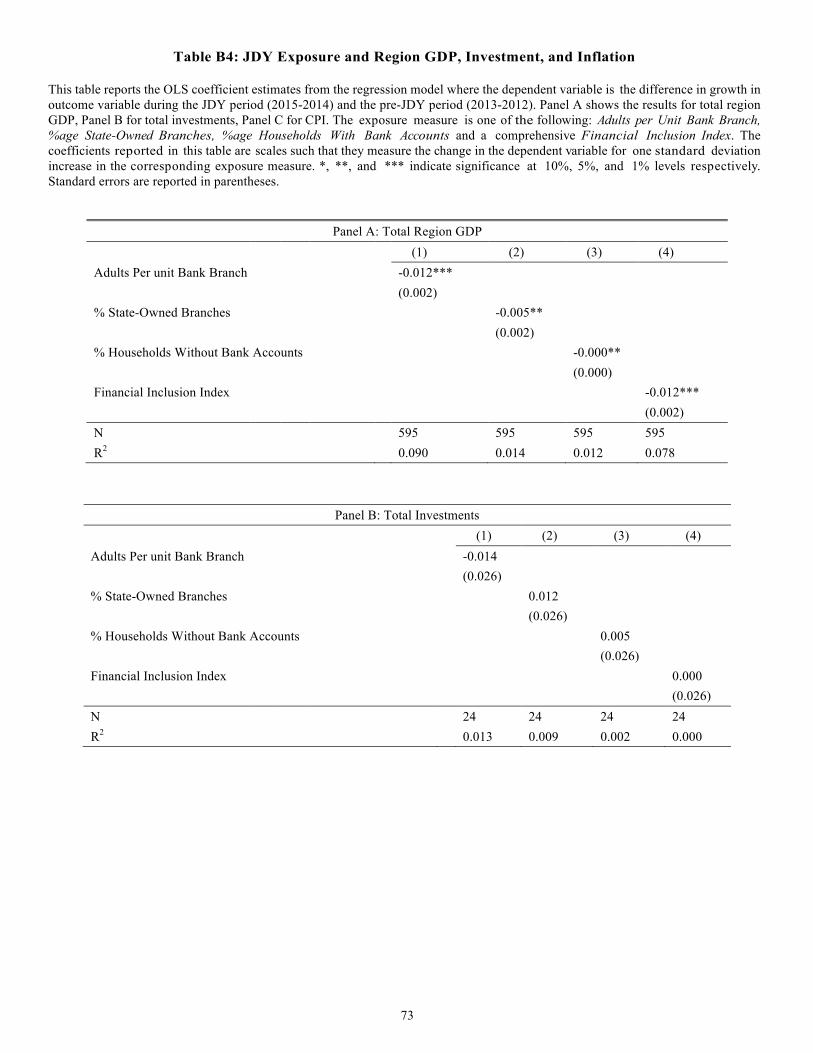
73

Table B4: JDY Exposure and Region GDP, Investment, and Inflation This table reports the OLS coefficient estimates from the regression model where the dependent variable is the difference in growth in outcome variable during the JDY period (2015-2014) and the pre-JDY period (2013-2012). Panel A shows the results for total region GDP, Panel B for total investments, Panel C for CPI. The exposure measure is one of the following: Adults per Unit Bank Branch, %age State-Owned Branches, %age Households With Bank Accounts and a comprehensive Financial Inclusion Index. The coefficients reported in this table are scales such that they measure the change in the dependent variable for one standard deviation increase in the corresponding exposure measure. *, **, and *** indicate significance at 10%, 5%, and 1% levels respectively. Standard errors are reported in parentheses.

Panel A: Total Region GDP

(1) (2) (3) (4) Adults Per unit Bank Branch -0.012***

(0.002) % State-Owned Branches -0.005**

(0.002) % Households Without Bank Accounts -0.000**

(0.000) Financial Inclusion Index -0.012*** (0.002) N 595 595 595 595 R2 0.090 0.014 0.012 0.078

Panel B: Total Investments

(1) (2) (3) (4) Adults Per unit Bank Branch -0.014

(0.026) % State-Owned Branches 0.012

(0.026) % Households Without Bank Accounts 0.005

(0.026) Financial Inclusion Index 0.000 (0.026) N 24 24 24 24 R2 0.013 0.009 0.002 0.000

74

Table B4 [continued]

Panel C: Total CPI

(1) (2) (3) (4) Adults Per unit Bank Branch 0.000

(0.003) % State-Owned Branches 0.000

(0.003) % Households Without Bank Accounts 0.002

(0.003) Financial Inclusion Index -0.001 (0.003) N 34 34 34 34 R2 0.000 0.000 0.019 0.001

75

Appendix C: Regional Distribution of Ex-Ante Program Exposure Measures

This figure shows the regional distribution of our four program exposure measures in India: Adults per Unit Bank Branch (Panel A), % State-Owned Branches (Panel B), Fraction of Households Without Bank Accounts (Panel C) and Financial Inclusion Index (Panel D). Higher values of all measures indicate lower levels of financial inclusion.

(a) Number of Adults per Unit Bank Branch (b) % State-Owned Branches

(c) Fraction of Households Without Bank Accounts (d) Financial Inclusion Index