B10a: Martingales through measure theory

Alison Etheridge

0 Introduction

0.1 Background

In the last fifty years probability theory has emerged both as a core mathematical discipline, sittingalongside geometry, algebra and analysis, and as a fundamental way of thinking about the world. Itprovides the rigorous mathematical framework necessary for modelling and understanding the inherentrandomness in the world around us. It has become an indispensible tool in many disciplines - fromphysics to neuroscience, from genetics to communication networks, and, of course, in mathematicalfinance. Equally, probabilistic approaches have gained importance in mathematics itself, from numbertheory to partial differential equations.

Our aim in this course is to introduce some of the key tools that allow us to unlock this mathematicalframework. We build on the measure theory that we learned in Part A Integration and develop themathematical foundations essential for more advanced courses in analysis and probability. We’ll thenintroduce the powerful concept of martingales and explore just a few of their remarkable properties.The nearest thing to a course text is

• David Williams, Probability with Martingales, CUP.

Also highly recommended are:

• S.R.S. Varadhan, Probability Theory, Courant Lecture Notes Vol. 7.

• R. Durrett, Probability: theory and examples, 4th Edition, CUP 2010.

• A. Gut, Probability: a graduate course, Springer 2005.

0.2 The Galton-Watson branching process

We begin with an example that illustrates some of the concepts that lie ahead.If you did Part A Probability then you’ll have already come across the Galton-Watson branching

process. In spite of earlier work by Bienayme, it is attributed to the great polymath Sir Frances Galtonand the Revd Henry Watson. Like many Victorians, Galton was worried about the demise of Englishfamily names. He posed a question in the Educational Times of 1873. He wrote

The decay of the families of men who have occupied conspicuous positions in past timeshas been a subject of frequent remark, and has given rise to various conjectures. Theinstances are very numerous in which surnames that were once common have become scarceor wholly disappeared. The tendency is universal, and, in explanation of it, the conclusionhas hastily been drawn that a rise in physical comfort and intellectual capacity is necessarilyaccompanied by a diminution in ‘fertility’. . .

1

He went on to ask “What is the probability that a name dies out by the ‘ordinary law of chances’?”Watson sent a solution which they published jointly the following year. The first step was to distill

the problem into a workable mathematical model and that model, formulated by Watson, is what wenow call the Galton-Watson branching process. Let’s state it formally:

Definition 0.1 (Galton-Watson branching process). Let X(m)r ;m, r ∈ N be a doubly infinite sequence

of independent identically distributed random variables, each with the same distribution as X, where

P[X = k] = pk, k = 0, 1, 2, . . .

and µ =∑∞

k=0 kpk < ∞. Write f(θ) =∑∞

k=0 pkθk for the probability generating function of X. Then

the sequence Znn∈N of random variables defined by

1. Z0 = 1,

2. Zn+1 = X(n+1)1 + · · · + X

(n+1)Zn

,

is the Galton-Watson branching branching process (started from a single ancestor) with offspring gen-erating function f .

The random variable Zn models the number of male descendants of a single male ancestor after ngenerations.

Claim 0.2. Let fn(θ) = E[θZn ]. Then fn is the n-fold composition of f with itself (where by conventiona 0-fold composition is the identity).

‘Proof’

We proceed by induction. First note that f0(θ) = θ, so f0 is the identity. Assume that fn = f · · ·fis an n-fold composition of f with itself. To compute fn+1, first note that

E[θZn+1

∣∣Zn = k]

= E

[θX

(n+1)1 +···+X

(n+1)k

]

= E

[θX

(n+1)1

]· · ·E

[θX

(n+1)k

](independence)

= f(θ)k,

(since X(n+1)i has the same distribution as X). Hence

E[θZn+1

∣∣Zn

]= f(θ)Zn . (1)

This is our first example of a conditional expectation. Notice that the right hand side of (1) is a randomvariable. Now

E[θZn+1

]= E

[E[θZn+1

∣∣Zn

]](2)

= E[f(θ)Zn

]

= fn (f(θ)) (inductive hypothesis).

2

In (2) we have used what is called the tower property of conditional expectataions. In this exampleyou can make all this work with the Partition Theorem of mods (because the events Zn = k partitionour space). In the general theory that follows, we’ll see how to replace the Partition Theorem whenthe sample space is not so nice.

Watson wanted to establish the extinction probability of the branching process, that is the value ofP[Zn = 0 for some n].

2

Claim 0.3. Let q = P[Zn = 0 for some n]. Then q is the smallest root in [0, 1] of the equation θ = f(θ).In particular,

• if µ = E[X] ≤ 1, then q = 1,

• if µ = E[X] > 1, then q < 1.

‘Proof’

Writing qn = P[Zn = 0], since Zn = 0 ⊆ Zn+1 = 0 we see that qn is an increasing function of nand, intuitively,

q = limn→∞

qn = limn→∞

fn(0). (3)

A proof will need the Monotone Convergence Theorem. Since fn+1(0) = f(fn(0)), evidently, granted (3),q solves q = f(q).

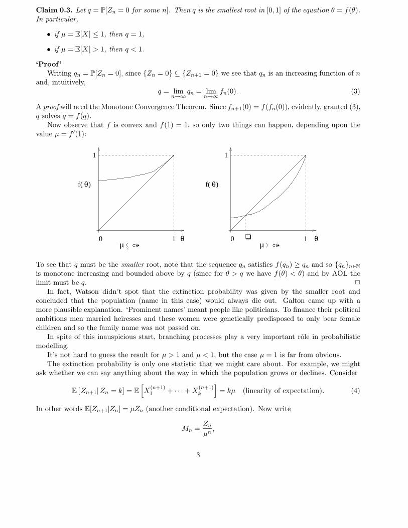
Now observe that f is convex and f(1) = 1, so only two things can happen, depending upon thevalue µ = f ′(1):

0 1

1

0 1

1

θ θ

θ)θ)f( f(

µ µ

To see that q must be the smaller root, note that the sequence qn satisfies f(qn) ≥ qn and so qnn∈N

is monotone increasing and bounded above by q (since for θ > q we have f(θ) < θ) and by AOL thelimit must be q. 2

In fact, Watson didn’t spot that the extinction probability was given by the smaller root andconcluded that the population (name in this case) would always die out. Galton came up with amore plausible explanation. ‘Prominent names’ meant people like politicians. To finance their politicalambitions men married heiresses and these women were genetically predisposed to only bear femalechildren and so the family name was not passed on.

In spite of this inauspicious start, branching processes play a very important role in probabilisticmodelling.

It’s not hard to guess the result for µ > 1 and µ < 1, but the case µ = 1 is far from obvious.The extinction probability is only one statistic that we might care about. For example, we might

ask whether we can say anything about the way in which the population grows or declines. Consider

E [Zn+1|Zn = k] = E

[X

(n+1)1 + · · · + X

(n+1)k

]= kµ (linearity of expectation). (4)

In other words E[Zn+1|Zn] = µZn (another conditional expectation). Now write

Mn =Zn

µn,

3

thenE [Mn+1|Mn] = Mn.

In fact, more is true.E [Mn+1|M0,M1, . . . ,Mn] = Mn.

The process Mnn∈N is our first example of a martingale.It is natural to ask whether Mn has a limit as n → ∞ and, if so, can we say anything about that

limit? We’re going to develop the tools to answer these questions, but for now, notice that for µ ≤ 1we have ‘proved’ that M∞ = limn→∞ Mn = 0 with probability one, so

0 = E[M∞] 6= limn→∞

E[Mn] = 1. (5)

We’re going to have to be careful in passing to limits, just as we discovered in Part A Integration.Indeed (5) may remind you of Fatou’s Lemma from Part A.

1 Measure spaces

We begin by recalling some definitions that we encountered in Part A Integration (and, less explicitly,in Mods Probability). The idea was that we wanted to be able to assign a ‘mass’ or ‘size’ to subsetsof a space in a consistent way. In particular, for us these subsets will be ‘events’ or ‘collections ofoutcomes’ (subsets of a probability sample space Ω) and the ‘mass’ will be a probability (a measure ofhow likely that event is to occur).

Definition 1.1 (Algebras and σ-algebras). Let Ω be a set and F a collection of subsets of Ω.

1. We say that F is an algebra if ∅ ∈ F and for all A,B ∈ F , Ac ∈ F and A ∪ B ∈ F ,

2. We say that F is a σ-algebra if ∅ ∈ F and for all sequences Ann∈N of elements of F , Ac1 ∈ F

and ∪n∈NAn ∈ F .

An algebra is closed under finite set operations whereas a σ-algebra is closed under countable setoperations.

Definition 1.2 (Measure space). We say that (Ω,F , µ) is a measure space if Ω is a set, F is a σ-algebra of subsets of Ω and µ : F → [0,∞] satisfies µ(∅) = 0 and for any sequence Ann∈N of disjointelements of F ,

µ

(∞⋃

n=1

An

)=

∞∑

n=1

µ(An). (6)

1. Given a measure space (Ω,F , µ), we say that µ is a finite measure if µ(Ω) < ∞.

2. If there is a sequence Enn∈N of sets from F with µ(En) < ∞ for all n and ∪n∈NEn = Ω, thenµ is said to be σ-finite.

3. In the special case when µ(Ω) = 1, we say that (Ω,F , µ) is a probability space and we often usethe notation (Ω,F , P) to emphasize this.

There are lots of measure spaces out there, several of which you are already familiar with.

4

Example 1.3 (Discrete measure theory). Let Ω be a countable set and F the power set of Ω (that isthe set of all subsets of Ω). A mass function is any function µ : Ω → [0,∞]. We can then define ameasure on Ω by µ(x) = µ(x) and extend to arbitrary subsets of Ω using Property (6).

Equally given a measure on Ω we can define a mass function. So there is a one-to-one correspon-dence between measures on a countable set Ω and mass functions.

These discrete measure spaces provide a ‘toy’ version of the general theory but in general they are notenough. Discrete measure theory is essentially the only context in which one can define the measureexplicitly. This is because σ-algebras are not in general amenable to an explicit presentation and it isnot in general the case that for an arbitrary set Ω all subsets of Ω can be assigned a measure - recallfrom Part A Integration that we constructed a non-Lebesgue measurable subset of R. Instead onespecifies the values to be taken by the measure on a smaller class of subsets of Ω that ‘generate’ theσ-algebra (as the singletons did in Example 1.3). This leads to two problems. First one needs to knowthat it is possible to extend the measure that we specify to the whole σ-algebra. This constructionproblem is often handled with Caratheodory’s Extension Theorem. The second problem is to know thatthere is only one measure on the σ-algebra that is consistent with our specification. This uniquenessproblem can often be resolved through a corollary of Dynkin’s π-system Lemma that we state below.First we need more definitions.

Definition 1.4 (Generated σ-algebras). Let A be a collection of subsets of Ω. Define

σ(A) = A ⊆ Ω : A ∈ F for all σ-algebras F containing A .

Then σ(A) is a σ-algebra (exercise) which is called the σ-algebra generated by A. It is the smallestσ-algebra containing A.

Example 1.5 (Borel σ-algebra, Borel measure, Radon measure). Let Ω be a topological space withtopology (that is open sets) T . Then the Borel σ-algebra of Ω is the σ-algebra generated by the opensets,

B(Ω) = σ(T ).

A measure µ on (Ω,B(Ω)) is called a Borel measure. If also µ(K) < ∞ for every compact set K ⊆ Ωthen µ is called a Radon measure.

Definition 1.6 (π-system). Let I be a collection of subsets of Ω. We say that I is a π-system if ∅ ∈ Iand for all A,B ∈ I, A ∩ B ∈ I.

Notice that an algebra is automatically a π-system.

Example 1.7. The collectionπ(R) = (−∞, x] : x ∈ R

form a π-system and σ(π(R)), the σ-algebra generated by π(R) is the Borel subsets of R (exercise).

Here’s why we care about π-systems.

Theorem 1.8 (Uniqueness of extension). Let Ω be a set and let I be a π-system on Ω. Let F = σ(I) bethe σ-algebra generated by I. Suppose that µ1, µ2 are measures on (Ω,F) such that µ1(Ω) = µ2(Ω) < ∞and µ1 = µ2 on I. Then µ1 = µ2 on F .

In particular, if two probability measures on Ω agree on a π-system, then they agree on the σ-algebragenerated by that π-system.

Exercise 1.9. Find an example where uniqueness fails if I is not a π-system on Ω = 1, 2, 3, 4.

5

That deals with uniqueness, but what about existence?

Definition 1.10 (Set functions). Let A be any set of subsets of Ω containing the emptyset ∅. A setfunction is a function µ : A → [0,∞] with µ(∅) = 0. Let µ be a set function. We say that µ is

1. increasing if for all A,B ∈ A with A ⊆ B,

µ(A) ≤ µ(B),

2. additive if for all disjoint A,B ∈ A with A ∪ B ∈ A (note that we must specify this in general)

µ(A ∪ B) = µ(A) + µ(B),

3. countably additive if for all sequences of disjoint sets Ann∈N in A with ∪n∈NAn ∈ A

µ

(⋃

n∈N

An

)=∑

n∈N

µ(An).

In this language, a measure space is a set Ω equipped with a σ-algebra F and a countably additiveset function on F .

An immediate consequence of σ-additivity of measures is the following useful lemma.Notation: For a sequence of sets Fnn∈N, Fn ↑ F means Fn ⊆ Fn+1 for all n and ∪n∈NFn = F .Similarly, Gn ↓ G means Gn ⊇ Gn+1 for all n and ∩n∈NGn = G.

Lemma 1.11 (Monotone convergence properties). Let (Ω,F , µ) be a measure space.

1. If Fnn∈N is a collection of sets from F with Fn ↑ F , then µ(Fn) ↑ µ(F ) as n → ∞,

2. If Gnn∈N is a collection of sets from F with Gn ↓ G, and µ(Gk) < ∞ for some k ∈ N thenµ(Gn) ↓ µ(G) as n → ∞.

Proof

1. Let H1 = F1, Hn = Fn\Fn−1, n ≥ 2. Then Hnn∈N are disjoint and

µ(Fn) = µ(H1 ∪ · · · ∪ Hn)

=n∑

k=1

µ(Hk) (additivity)

↑∞∑

k=1

µ(Hk) (positivity)

= µ

(∞⋃

k=1

Hk

)(σ-additivity)

= µ(F ).

2. follows on taking Fn = Gk\Gk+n. 2

Note that µ(Gk) < ∞ is essential (for example take Gn = (n,∞) ⊆ R and Lebesgue measure).

Theorem 1.12 (Caratheodory Extension Theorem). Let Ω be a set and A an algebra on Ω. LetF = σ(A) denote the σ-algebra generated by A. Let µ0 : A → [0,∞] be a countably additive setfunction. Then there exists a measure µ on (Ω,F) such that µ = µ0 on A.

6

Remark 1.13. If µ0(Ω) < ∞, then Theorem 1.8 tells us that µ is unique since an algebra is certainlya π-system.

Corollary 1.14. There exists a unique measure µ on the Borel subsets of R such that for all a, b ∈ R

with b > a, µ ((a, b]) = b − a. The measure µ is the Lebesgue measure on B(R).

The proof of this result is an exercise. (The tricky bit is that Theorem 1.8 requires µ(Ω) < ∞ and soyou must work a little harder.)

The proof of the Caratheordory Extension Theorem proceeds in much the same way as our (sketch)proof of the existence of Lebesgue measure in Part A Integration. First one defines an outer measureµ∗ by

µ∗(A) = inf∑

j

µ0(Aj) : A ⊆ ∪j∈NAj, Aj ∈ A

and define a set to be measurable if for all sets E,

µ∗(A) = µ∗(A ∩ E) + µ∗(A ∩ Ec).

One must check that µ∗ then defines a countably additive set function on the collection of measurablesets and that the measurable sets form a σ-algebra that contains A. For more details see Varadhanand the references therein.

The Caratheodory Extension Theorem doesn’t quite solve the problem of constructing measures onσ-algebras - it reduces it to constructing countably additive set functions on algebras. The followingtheorem is very useful for constructing probability measures on Borel subsets of R. First we need somenotation.Notation:

For −∞ ≤ a < b < ∞, let Ia,b = (a, b] and set Ia,∞ = (a,∞)Let I = Ia,b : −∞ ≤ a < b ≤ ∞. That is I is the collection of intervals that are open on the left

and closed on the right.Now suppose that F : R → [0, 1] is a non-decreasing function with limx→−∞ F (x) = 0 and

limx→∞ F (x) = 1. Recall that F is said to be right continuous if for each x ∈ R F (x) = limy↓x F (y).Given such an F we can define a finitely additive probability measure on the algebra A consisting ofthe emptyset and finite disjoint unions of intervals from I by setting

µ(Ia,b) = F (b) − F (a)

for intervals and then extending it to A by defining it as the sum for disjoint unions from I.Notice that the Borel σ-field B(R) is the σ-field generated by A. So Caratheodory’s Extension

Theorem tells us that this extends to a probability measure on B provided that µ is countably additiveon A.

Theorem 1.15 (Lebesgue). µ is countably additive on A if and only if F (x) is a right continuousfunction of x. Therefore for each right continuous non-decreasing function F (x) with F (−∞) = 0and F (∞) = 1 there is a unique probability measure µ on the Borel sets of the line such that F (x) =µ(I−∞,x). Conversely, every countably additive probability measure µ on B(R) comes from some F .The correspondence is one-to-one.

Sketch of key points of proof

We’ll see essentially this result again in a slightly different guise later in the course. Rather thangive a detailed proof here, let’s see where right continuity comes into it.

7

First note that by the monotone convergence properties of Lemma 1.11 (as you prove on problemsheet 1) the σ-additivity of µ on A is equivalent to saying that for any sequence Ann∈N of sets fromA with An ↓ ∅, µ(An) ↓ 0.

If µ is σ-additive, then right continuity of F is immediate since this implies

µ(Ixy) = F (y) − F (x) ↓ 0 as y ↓ x.

The other way round is a bit more work. Suppose that F is right continuous but, for a contradiction,that there exist Ann∈N from A with µ(An) ≥ δ > 0 and An ↓ ∅.

Step 1: Replace An by Bn = An ∩ [−l, l]. Since

|µ(An) − µ(Bn)| ≤ 1 − F (l) + F (−l),

we may do this in such a way that µ(Bn) ≥ δ/2 > 0.Step 2: Supose that Bn = ∪kn

i=1Iani,bni

. Replace Bn by Cn = ∪kn

i=1Iani,bni

where ani< ani

< bniand

we use right continuity of F to do this in such a way that

µ(Bn\Cn) <δ

10 · 2nfor each n.

Step 3: Set Dn = Cn, the closure of Cn (obtained by adding the points anito Cn). Set En = ∩n

i=1Dni

and Fn = ∩ni=1Ci. Then

Fn ⊆ En ⊆ An.

So En ↓ ∅ (since An ↓ ∅). But

µ(Fn) ≥ µ(Bn) −∑

i

µ(Bi\Ci) =δ

2−∑

i

δ

10 · 2i=

2δ

5

and so Fn and hence Dn is non-empty. The decreasing limit of a sequence of closed sets cannot beempty and so we have the desired contradiction. 2

The function F (x) is the distribution function corresponding to the probability measure µ. In thecase when it is differentiable it is precisely the cumulative distribution function of a continuous randomvariable with probability density function f(x) = F ′(x) that we encountered in mods.

If x1, x2, . . . is a sequence of points and we have probabilities pn at these points (for examplex1, x2, . . . could be the non-negative integers), then for the discrete measure

µ(A) =∑

n:xn∈A

pn,

we have the distribution functionF (x) =

∑

n:xn≤x

pn,

which only increases by jumps, the jump at xn being of height pn.There are examples of continuous F that don’t come from any density (recall the Devil’s staircase

of Part A Integration).The measure µ is sometimes called a Lebesgue-Stieltjes measure. We’ll return to it a little later.We now have a very rich class of measures to work with. In Part A Integration, we developed a

theory based on Lebesgue measure. It is natural to ask whether we can develop an analogous theoryfor other measures. The answer is ‘yes’ and it is gratifying that we already did the work in Part A.The proofs that we used there will carry over to any σ-finite measure. It is left as a (useful) exerciseto check that. Here we just state the key definitions and results.

8

2 Integration

2.1 Definition of the integral

Definition 2.1 (Measurable function). Let (Ω,F , µ) and (Λ,G, ν) be measure spaces. A functionf : Ω → Λ is measurable (with respect to F , G) if and only if

G ∈ G =⇒ f−1(G) ∈ F .

Let (Ω,F , µ) be a measure space. We suppose that [−∞,∞] is endowed with the Borel sets B(R).We want to define, where possible, for measurable functions f : Ω → [−∞,∞], the integral of f withrespect to µ,

µ(f) =

∫fdµ =

∫

x∈Ωf(x)µ(dx).

Unless otherwise stated, measurable functions map to R with the Borel σ-algebra.Recall that

lim supn→∞

xn = limn→∞

supm≥n

xm and lim infn→∞

xn = limn→∞

infm≥n

xm.

Theorem 2.2. Let fnn∈N be a sequence of measurable functions with respect to F ,B). Then thefollowing are also measurable:

maxn≤k

fn, minn≤k

fn, supn∈N

fn, infn∈N

fn, lim supn→∞

fn, lim infn→∞

fn.

Definition 2.3. A simple function is a finite sum

φ(x) =

N∑

k=1

ak1Ek(x) (7)

where each Ek is a measurable set of finite measure and the ak are constants.

The canonical form of a simple function φ is the unique decomposition as in (7) where the numbersak are distinct and the sets Ek are disjoint.

Definition 2.4. If φ is a simple function with canonical form

φ(x) =

M∑

k=1

ck1Fk(x)

then we define the integral of φ with respect to µ as

∫φ(x)µ(dx) =

M∑

k=1

ckµ(Fk).

Definition 2.5. For a non-negative measurable function f on (Ω,F , µ) we define the integral

µ(f) = supµ(g) : g simple, g ≤ f

.

Definition 2.6. We say that a measurable function f on (Ω,F , µ) is integrable if µ(|f |) < ∞ and thenwe set

µ(f) = µ(f+) − µ(f−).

Definition 2.7 (µ-almost everywhere). Let (Ω,F , µ) be a measure space. We say that a property holdsµ-almost everywhere if it holds except on a set of µ-measure zero. If µ is a probability measure, weoften say almost surely instead of almost everywhere.

Note: It is vital to remember that notions of almost everywhere depend on the underlying measure µ.

9

2.2 The Convergence Theorems

Theorem 2.8 (Fatou’s Lemma). Let fnn≥1 be a sequence of non-negative measurable functions on(Ω,F , µ). Then

µ(lim infn→∞

fn) ≤ lim infn→∞

µ(fn).

Corollary 2.9 (Reverse Fatou Lemma). Let fnn≥1 be a sequence of non-negative integrable functions.Assume that there exists a measurable function g ≥ 0 such that µ(g) < ∞ and fn ≤ g for all n ∈ N.Then

µ(lim supn→∞

fn) ≥ lim supn→∞

µ(fn).

Proof

Apply Fatou to g − fnn≥1. (Note that µ(g) < ∞ is needed.) 2

Theorem 2.10 (Monotone Convergence Theorem). Let fnn≥1 be a sequence of non-negative mea-surable functions. Then

fn ↑ f =⇒ µ(fn) ↑ µ(f).

(Note that we are not excluding µ(f) = ∞ here.)

Theorem 2.11 (Dominated Convergence Theorem). Let fnn≥1 be a sequence of integrable functionson (Ω,F , µ) with fn(x) → f(x) as n → ∞ for each x ∈ Ω. (We say that fn converges pointwise to f .)Suppose that for some integrable function g, |fn| ≤ g for all n. Then f is integrable and

µ(fn) → µ(f) as n → ∞.

A useful lemma that you prove on the problem sheet is the following.

Lemma 2.12 (Scheffe’s Lemma). Let fnn≥1 be a sequence of non-negative integrable functions on(Ω,F , µ) and suppose that fn(x) → f(x) for µ-almost every x ∈ Ω (written fn → f a.e.). Then

µ(|fn − f |) n→∞−→ 0 iff µ(fn)n→∞−→ µ(f).

The corollaries of the MCT and DCT for series also extend to this general setting.The measurable functions that are going to interest us most in what follows are random variables.

Definition 2.13 (Random Variable). In the special case when (Ω,F , P) is a probability space, we’llcall a measurable map X : Ω → R a random variable.

In the language of mods, Ω is the sample space of an experiment and the random variable X is ameasurement of the outcome of the experiment. We can think of X as inducing a probability measureon R via

µX(A) = P[X−1(A)] for A ∈ B(R),

and, in particular, FX(x) = µX((−∞, x]) defines the distribution function of X (c.f. Theorem 1.15).Since (−∞, x] : x ∈ R is a π-system, we see that the distribution function uniquely determines µX .In this notation, ∫

X(ω)P(dω) =

∫xµX(dx) ≡ E[X].

Very often in applications we suppress the sample space and work directly with µX .In fact this idea of using a measurable function to map a measure on one space onto a measure on

another is more general. Let (Ω,F) and (Λ,G) be measurable spaces and let µ be a measure on F .

10

Then any measurable (with respect to (F ,G)) function f : Ω → Λ induces an image measure ν = µf−1

on G given byν(A) = µ

(f−1(A)

).

On the problem sheet you’ll use this to construct the measure µ of Theorem 1.15 from Lebesgue measureon [0, 1].

2.3 Product Spaces and Independence

Because we want to be able to discuss more than one random variable at a time, we need the notionof product spaces.

Definition 2.14 (Product σ-algebras). Given two sets Ω1 and Ω2, the Cartesian product Ω = Ω1×Ω2

is the set of pairs (ω1, ω2) with ω1 ∈ Ω1 and ω2 ∈ Ω2.If Ω1 and Ω2 come with σ-algebras F1 and F2 respectively, then we can define a natural σ-algebra

F on Ω as the σ-algebra generated by sets of the form A1 × A2 with A1 ∈ F1 and A2 ∈ F2. Thisσ-algebra will be called the product σ-algebra.

Given two probability measures P1 and P2 on (Ω1,F1) and (Ω2,F2) respectively, we’d like to definea probability measure on (Ω,F) by

P[A1 × A2] = P1[A1] × P2[A2] (8)

and extending it to the whole of F .Evidently it can be extended to the algebra A of sets that are finite disjoint unions of measurable

rectangles as the obvious sum. It is a tedious, but straightforward, exercise to check that this iswell-defined.

To check that we can extend it to the whole of F = σ(A), we need to check that P defined by (8)is actually countably additive on A so that we can apply Caratheodory’s Extension Theorem.

Lemma 2.15. The finitely additive set function P, defined on A through (8) is countably additive onA.

Proof

Recall that countable additivity is equivalent to checking that for any sequence of measurable setswith An ↓ ∅, P[An] ↓ 0.

For any A ∈ A, define the section

Aω2 = ω1 : (ω1, ω2) ∈ A.

Then P1[Aω2 ] is a measurable function of ω2 (in fact it is a simple function - exercise) and

P[A] =

∫

Ω2

P1[Aω2 ]dP2.

Now let An ∈ A be a sequence of sets with An ↓ ∅. Then

An,ω2 = ω1 : (ω1, ω2) ∈ An

satisfies An,ω2 ↓ ∅ for each ω2 ∈ Ω2. Since P1 is countably additive, P1[An,ω2] → 0 for each ω2 ∈ Ω2

and since 0 ≤ P1[An,ω2 ] ≤ 1 for n ≥ 1 it follows from the DCT (with dominating function g ≡ 1) that

P[An] =

∫P1[An,ω2]dP2 → 0.

11

So P is countably additive as required. 2

By an application of the Caratheodory Extension Theorem we see that P extends uniquely to acountably additive set function on σ(A) = F .

Definition 2.16 (Product measure). The measure P defined through (8) is called the product measureon (Ω,F).

The most familiar example of a product measure is, of course, Lebesgue measure on R2, or, moregenerally, by extending the above in the obvious way on Rd.

Our integration theory was valid for any measure space (Ω,F , µ) on which µ is a countably additivemeasure. But as we already know for R2, in order to calculate the integral of a function of two variablesit is convenient to be able to proceed in stages and calculate the repeated integral. So if f is integrablewith respect to Lebesgue measure on R2 then we know that

∫

R2

f(x, y)dxdy =

∫ (∫f(x, y)dx

)dy =

∫ (∫f(x, y)dy

)dx.

What is the analogous result here?

Theorem 2.17 (Fubini’s Theorem). Let f(ω) = f(ω1, ω2) be a measurable function on (Ω,F). Thenf can be considered as a function of ω2 for each fixed ω1 or the other way around. The functions gω1(·)on Ω2 and hω2(ω1) on Ω1 defined by

gω1(ω2) = hω2(ω1) = f(ω1, ω2)

are measurable for each ω1 and ω2.If f is integrable with respect to the product measure P then the function gω1(·) is integrable with

respect to P2 for P1-almost every ω1 and the function hω2(·) is integrable with respect to P1 for P2-almostevery ω2. Their integrals

G(ω1) =

∫

Ω2

gω1(ω2)dP2

and

H(ω2) =

∫

Ω1

hω2(ω1)dP1

are measurable, finite almost everywhere, and integrable with respect to P1 and P2 respectively. Finally,

∫

Ωf(ω1, ω2)dP =

∫

Ω1

G(ω1)dP1 =

∫

Ω2

H(ω2)dP2.

Conversely, for a non-negative function, if either∫

GdP1 or∫

HdP2 is finite then so is the other andf is integrable with integral equal to either of the repeated integrals.

Warning: Just as we saw for functions on R2 in Part A Integration, for f to be integrable we requirethat |f | is integrable. If we drop the assumption of non-negative in the last part then the result is falseand it is not hard to cook up examples where both repeated integrals exist but f is not integrable.

The proof of Fubini’s Theorem is not examinable. It follows a standard pattern that Williams callsthe standard machine:

• Check the result for f = 1A where A ∈ F .

• Extend by linearity to non-negative simple functions.

12

• Pass to increasing limits using the MCT.

• Take positive and negative parts.

However, in this case, it turns out that what one might hope would be the easy bit - checking theresult for indicator functions of measurable sets - is highly non-trivial. It relies on a result called theMonotone Class Theorem. We include this here, but it is not examinable.

Definition 2.18 (Monotone Class). A family of subsets M of Ω is called a monotone class if it isstable under countable unions and countable intersections.

Theorem 2.19 (The Monotone Class Theorem). The smallest monotone class containing an algebraA is the σ-algebra generated by A.

The point is that if we have a result that we know to be valid on an algebra A and we can checkthat the sets for which the result holds form a monotone class, then necessarily the result holds onσ(A).

To illustrate, here’s the difficult bit of the proof of Fubini’s Theorem.

Corollary 2.20 (to Lemma 2.15). For and A ∈ F , if we denote by Aω1 and Aω2 the respective sections

Aω1 = ω2 : (ω1, ω2) ∈ A,

Aω2 = ω1 : (ω1, ω2) ∈ A,then the functions P1[Aω2 ] and P2[Aω1 ] are measurable and

P[A] =

∫P1[Aω2 ]dP2 =

∫P2[Aω1 ]dP1.

In particular, for a measurable set A, P[A] = 0 iff for P1-almost all ω1 the sections Aω1 have P2-measurezero or equivalently for P2-almost every ω2, the sections Aω2 have P1-measure zero.

Proof

The assertion clearly works for a rectangle of the form A1 ×A2 with A1 ∈ F1 and A2 ∈ F2. It alsofollows by simple addition to sets in A. By the MCT, the class of sets for which the assertion is validform a monotone class, and since it contains A it also contains σ(A) = F . 2

One of the central ideas in probability theory is independence and this is intricately linked withproduct measure.

Intuitively, two events are independent if they have no influence on each other. Knowing that onehas happened tells us nothing about the chance that the other has happened. More formally:

Definition 2.21 (Independence). Let (Ω,F , P) be a probability space. Let I be a finite or countablyinfinite set. We say that the events Ai ∈ F , i ∈ I are independent if for all finite subsets J ⊆ I

P

[⋂

i∈J

Ai

]=∏

i∈J

P[Ai].

Sub σ-algebras G1,G2, . . . of F are called independent if whenever Gi ∈ Gi (i ∈ N) and i1, i2, . . . , in aredistinct

P[Gi1 ∩ . . . Gin ] =n∏

k=1

P[Gik ].

13

How does this fit in with our notion of independence from mods?

Definition 2.22 (σ-algebra generated by a random variable). Let (Ω,F , P) be a probability spaceand let X be a real-valued random variable on Ω,F , P) (that is a measurable function from Ω,F) to(R,B(R)). Then

σ(X) = σ (ω ∈ Ω : X(ω) ∈ A;A ∈ B(R))= σ

(X−1(A) : A ∈ B(R)

).

It is the smallest sub σ-algebra of F with respect to which X is a measurable function.

Definition 2.23 (Independent random variables). Random variables X1,X2, . . . are called independentif the σ-algebras σ(X1), σ(X2), . . . are independent.

If we write this in more familiar language we see that X and Y are independent if for each pairA,B of Borel subsets of R

P[X ∈ A,Y ∈ B] = P[X ∈ A]P[Y ∈ B].

From this it is easy to check the following result.

Lemma 2.24. Two random variables X and Y on the probability space (Ω,F , P) are independent iffthe measure µXY induced on R2 by (X,Y ) is the product measure µX × µY where µX and µY are themeasures on R induced by X and Y respectively.

This generalises the result you learned in mods and part A for discrete/continuous random variables- two continuous random variables X and Y are independent if and only if their joint density functioncan be written as the product of the density function of X and the density function of Y .

Of course the conditions of Definition 2.23 would be impossible to check in general - we don’thave a nice explicit presentation of the σ-algebras σ(Xi). But we can use our result of Theorem 1.8(uniqueness of extension) to reduce it to something much more manageable.

Theorem 2.25. Let (Ω,F , P) be a probability space. Suppose that G and H are sub σ-algebras of Fand that G0 ad H0 are π-systems with

σ(G0) = G, and σ(H0) = H.

Then G and H are independent iff G0 and H0 are independent, i.e. P[G ∩ H] = P[G]P[H] wheneverG ∈ G0, H ∈ H0.

Proof

The two measures H 7→ P[G∩H] and H 7→ P[G]P[H] on (Ω,H) have the same total mass P[G] andthey agree on the π-system H0. So by Theorem 1.8 they agree on σ(H0) = H. Hence, for G ∈ G0 andH ∈ H

P[G ∩ H] = P[G]P[H].

Now fix H ∈ H and repeat the argument with the two measures G 7→ P[G∩H] and G 7→ P[G]P[H]. 2

Corollary 2.26. A sequence Xnn∈N of real-valued random variables on (Ω,F , P) is independent ifffor all x1, . . . xn ∈ R and n ∈ N

P[X1 ≤ x1, . . . Xn ≤ xn] = P[X1 ≤ x1] . . . P[Xn ≤ xn].

14

Remark 2.27 (Kolmogorov’s Consistency Theorem). Notice that our notion of independence onlyreally makes sense if our random variables are defined on a common probability space. For a countablesequence of random variables with specified distributions it is not completely clear that there exists sucha probability space.

By extending our construction of product measure in the obvious way, we can construct a measureon Rn for every n which is the joint distribution of the first n of the random variables. Let us denoteit by Pn. The Pn’s are consistent in the sense that if we project from R(n+1) to Rn in the obvious way,then Pn+1 projects to Pn. Such a family is called a consistent family of finite dimensional distributions.

Now look at the space Ω = R∞ of all real sequences ω = xn : n ≥ 1 with the σ-algebra F , generatedby the algebra A of finite dimensional cylinder sets, that is sets of the form B = ω : (x1, . . . , xn) ∈ Awhere A varies over the Borel sets in Rn and n varies over positive integers.

The Kolmogorov Consistency Theorem tells us that given a consistent family of finite dimensionaldistributions Pn, there exists a unique P on (Ω,F) such that for every n, under the natural projectionπn(ω) = (x1, . . . , xn), the induced measure Pπ−1

n = Pn on Rn.

3 Tail events and modes of convergence

3.1 The Borel-Cantelli Lemmas

We’ll return to independence, or more importantly lack of it, in the next section, but first we lookat some ramifications of our theory of integration for probability theory. Throughout, (Ω,F , P) willdenote a probability space.

First we’re going to look at Fatou’s Lemma in this setting, but in the special case where the functionsfn are indicator functions of measurable sets. Recall that Fatou’s Lemma says that for a sequence ofnon-negative measurable functions fnn∈N

P[lim infn→∞

fn] ≤ lim infn→∞

P[fn]

and the reverse Fatou lemma says that if 0 ≤ fn ≤ g for some g with P[g] < ∞ then

P[lim supn→∞

fn] ≥ lim supn→∞

P[fn].

So what does lim infn→∞ fn or lim supn→∞ fn look like if the fn’s are indicator functions of sets?Let fn = 1An for some An ∈ F .

lim supn→∞

fn = limn→∞

supm≥n

fm

= limn→∞

supm≥n

1Am

= limn→∞

1∪m≥nAm

= 1∩n∈N∪m≥nAm .

This motivates the following definition.

Definition 3.1. Let Ann∈N be a sequence of sets from F . We define

lim supn→∞

An =⋂

n∈N

∪m≥nAm

= Am occurs infinitely often= ω ∈ Ω : ω ∈ Am for infinitely many m.

15

lim infn→∞

An =⋃

n∈N

∩m≥nAm

= ω ∈ Ω : for some m(ω), ω ∈ Am for all m ≥ m(ω)= ‘Am eventually’= Ac

m infinitely oftenc.

Lemma 3.2.

1lim supn→∞ An= lim sup

n→∞1An , 1lim infn→∞ An

= lim infn→∞

1An .

The proof is an exercise (based on our calculations above).In this terminology the Fatou and reverse Fatou Lemmas say

P[An eventually] ≤ lim infn→∞

P[An]

andP[An i.o.] ≥ lim sup

n→∞P[An]

(both of which make good intuitive sense). In fact we can say more about the probabilities of theseevents.

Lemma 3.3 (The First Borel-Cantelli Lemma, BC1). Suppose that

∑

n∈N

P[An] < ∞,

thenP[An i.o.] = 0.

Remark 3.4. Notice that we are making no assumptions about independence here. This is a verypowerful result.

Proof of BC1

Let Gn = ∪m≥nAm. Then

P[Gn] ≤∞∑

m=n

P[Am]

and Gn ↓ G = lim supn→∞ An, so by Lemma 1.11 (monotone convergence properties), P[Gn] ↓ P[G].On the other hand, since

∑n∈N P[An] < ∞, we have that

∞∑

m=n

P[Am] → 0 as n → ∞,

and soP[lim sup

n→∞An] = lim

n→∞P[Gn] = 0

as required. 2

A partial converse to this result is provided by the second Borel-Cantelli Lemma, but note that wemust now assume that the events are independent.

16

Lemma 3.5 (The Second Borel-Cantelli Lemma, BC2). Assume that Ann∈N are independent events.If ∑

n∈N

P[An] = ∞

thenP[An i.o.] = 1.

Proof

Set am = P[Am] and note that 1−a ≤ e−a. We consider the complementary event Acn eventually.

P[⋂

m≥n

Acm] =

∏

m≥n

(1 − am) (by independence)

≤ exp(−∑

m≥n

am) = 0.

Hence using Lemma 1.11 (monotone convergence properties) again

P

⋃

n∈N

⋂

m≥n

Acm

= lim

N→∞P

N⋃

i=1

⋂

m≥n

Acm

≤ limN→∞

N∑

n=1

P

⋂

m≥n

Acm

= 0.

Thus

P

[lim infn→∞

Acn

]= P

⋃

n∈N

⋂

m≥n

Acm

= 0.

and since (lim infn→∞

Acn

)c= lim sup

n→∞An

we haveP[lim sup

n→∞An] = P[An i.o.] = 1

as required. 2

Example 3.6. A monkey is provided with a typewriter. At each time step it has probability 1/26of typing any of the 26 letters independently of other times. What is the probability that it will typeABRACADABRA at least once? infinitely often?

Solution

We can consider the events

Ak = ABRACADABRA is typed between times 11k + 1 and 11(k + 1)

for each k. The events are independent and P[Ak] = (1/26)11 > 0. So∑∞

k=1 P[Ak] = ∞. Thus BC2says that Ak happens infinitely often. 2

Later in the course, with the help of a suitable martingale, we’ll be able to work out how long wemust wait, on average, before we see patterns appearing in the outcomes of a series of independentexperiments.

We’ll see many applications of BC1 and BC2 in what follows. Before developing more machinery,here is one more.

17

Example 3.7. Let Xnn≥1 be independent exponentially distributed random variables with mean 1and let Mn = maxX1, . . . ,Xn. Then

P

[lim infn→∞

Mn

log n≥ 1

]= 1.

Remark 3.8. In fact with a little more work we can show that

P

[Mn

log n→ 1 as n → ∞

]= 1.

See, for example, S.C. Port, Theoretical Probability for Applications, Wiley 1993, Example 4.7.2 p.560.

First recall that if X is an exponential random variable with parameter 1 then

P[X ≤ x] =

0 x < 0,

1 − e−x x ≥ 0.

Fix 0 < ǫ < 1. Then

P[Mn ≤ (1 − ǫ) log n] = P

[n⋂

i=1

Xi ≤ (1 − ǫ) log n]

=n∏

i=1

P [Xi ≤ (1 − ǫ) log n] (independence)

=

(1 − 1

n1−ǫ

)n

≤ exp(−nǫ).

Thus∞∑

n=1

P[Mn ≤ (1 − ǫ) log n] < ∞

and so by BC1P[Mn ≤ (1 − ǫ) log n i.o.] = 0.

Since ǫ was arbitrary this gives

P

[lim infn→∞

Mn

log n≥ 1

]= 1.

2

At first sight, it looks as though BC1 and BC2 are not very powerful - they tell us when certainevents have probability zero or one. But in fact for many applications, in particular when the eventsare independent, these are events that can only have probability zero or one. This is because they areexamples of what are known as ‘tail’ events.

Recall from Definition 2.22 that the σ-algebra generated by a random variable X is the smallestsub σ-algebra of F with respect to which X is measurable. That is

σ(X) = σ(X−1(A) : A ∈ B(R)

).

Definition 3.9 (Tail σ-algebra). For a sequence of random variables Xnn∈N define

Tn = σ(Xn+1,Xn+2 . . .)

andT =

⋂

n∈N

Tn.

Then T is called the tail σ-algebra of the sequence Xnn∈N.

18

We can think of the tail σ-algebra as containing events describing the limiting behaviour of thesequence as n → ∞.

Theorem 3.10 (Kolmogorov’s 0-1 law). Let Xnn∈N be a sequence of independent random variables.Then the tail σ-algebra T of Xnn∈N contains only events of probability 0 or 1. Moreover, any T -measurable random variable is almost surely constant.

Proof

Let Fn = σ(X1, . . . ,Xn). Note that Fn is generated by the π-system of events

A = X1 ≤ x1, . . . ,Xn ≤ xn : x1, . . . , xn ∈ R

and Tn is generated by the π-system of events

B = Xn+1 ≤ xn+1, . . . ,Xn+k ≤ xn+k : xn+1, . . . , xn+k ∈ R, k ∈ N .

For any A ∈ A, B ∈ B, by the independence of the random variables Xnn∈N, we have

P[A ∩ B] = P[A]P[B]

and so by Theorem 2.25 the σ-algebras σ(A) = Fn and σ(B) = Tn are also independent.Since T ⊆ Tn we conclude that Fn and T are also independent.Now ∪n∈NFn is a π-system (although not in general a σ-algebra) generating the σ-algebra F∞ =

σ(Xnn∈N). So applying Theorem 2.25 again we see that F∞ and T are independent. But T ⊆ F∞

so that if A ∈ TP[A] = P[A ∩ A] = P[A]2

and so P[A] = 0 or P[A] = 1.Now suppose that Y is any T -measurable random variable. Then FY (y) = P[Y ≤ y] is right

continuous and takes only values in 0, 1. So P[Y = c] = 1 where c = infy : FY (y) = 1. 2

Example 3.11. Let Xnn∈N be a sequence of independent, identically distributed (i.i.d.) randomvariables and let Zn =

∑nk=1 Xk. Consider L = lim supn→∞ Zn/n. Then L is a tail random variable and

so almost surely constant. We’ll prove later in the course (Theorem 9.2) that, under weak assumptions,L = E[X1] almost surely.

If the Xn in the last example have mean zero one, then setting

B =

lim sup

n→∞

Zn√2n log log n

= 1

, (9)

similarly we have P[B] = 0 or P[B] = 1. In fact P[B] = 1. This is called the law of the iteratedlogarithm. Under the slightly stronger assumption that ∃α > 0 such that E[|Xn|2+α] < ∞, Varadhanproves this by a (delicate) application of Borel-Cantelli.

You may at this point be feeling a little confused. In mods probability/statistics (possibly evenat school) you learned that if Xnn∈N is a sequence of i.i.d. random variables with mean zero andvariance one then

P

[X1 + · · · + Xn√

n≤ a

]= P

[Zn√

n≤ a

]n→∞−→

∫ a

−∞

1√2π

exp

(−x2

2

)dx. (10)

This is the Central Limit Theorem without which statistics would be a very different subject. Howdoes it fit with (9)? The results (9) and (10) are giving quite different results about the behaviour ofZn for large n. They correspond to different ‘modes of convergence’.

19

Definition 3.12 (Modes of convergence). Let (Ω,F , P) be a probability space, X a given randomvariable and Xnn∈N a sequence of random variables.

1. We say that Xnn∈N converges almost surely to X (written Xna.s.→ X) if

P[ω : limn→∞

Xn(ω) = X(ω)] = 1.

2. We say that Xnn∈N converges to X in probability (written XnP→ X) if, given ǫ > 0,

limn→∞

P[ω : |Xn(ω) − X(ω)| > ǫ] = 0.

3. Let F and Fn denote the distribution functions of X and Xn respectively. We say that Xn

converges to X in distribution (written Xnd→ X or Xn

L→ X) if

limn→∞

Fn(x) = F (x).

4. Suppose that X and Xn have finite rth moment for some r > 0 (that is E[|X|r] < ∞). We say

that Xn converges to X in Lr (written XnLr

→ X) if

limn→∞

E[|Xn − X|r] = 0.

These notions of convergence are all different.

Convergence a.s. =⇒ Convergence in Probability =⇒ Convergence in Distribution

⇑Convergence in Lr

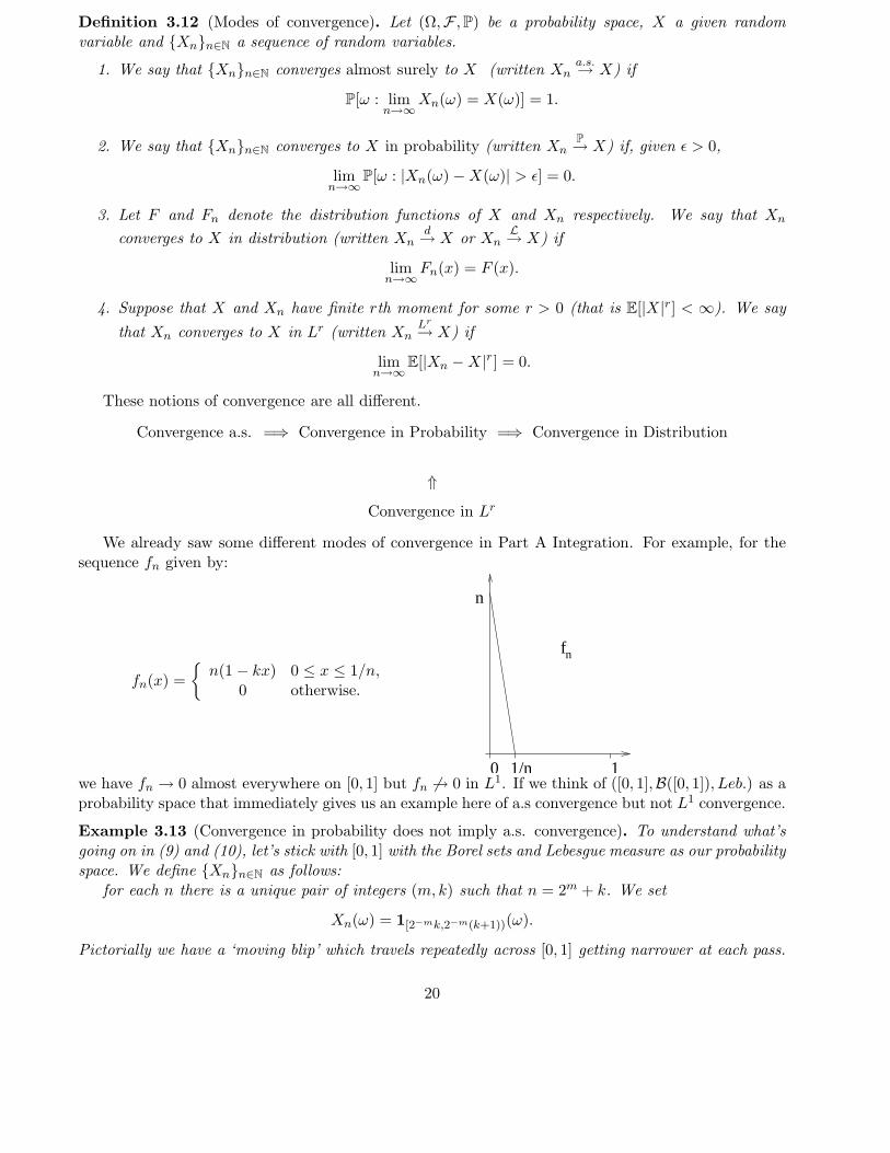
We already saw some different modes of convergence in Part A Integration. For example, for thesequence fn given by:

fn(x) =

n(1 − kx) 0 ≤ x ≤ 1/n,

0 otherwise.

f

10

n

n

1/nwe have fn → 0 almost everywhere on [0, 1] but fn 6→ 0 in L1. If we think of ([0, 1],B([0, 1]), Leb.) as aprobability space that immediately gives us an example here of a.s convergence but not L1 convergence.

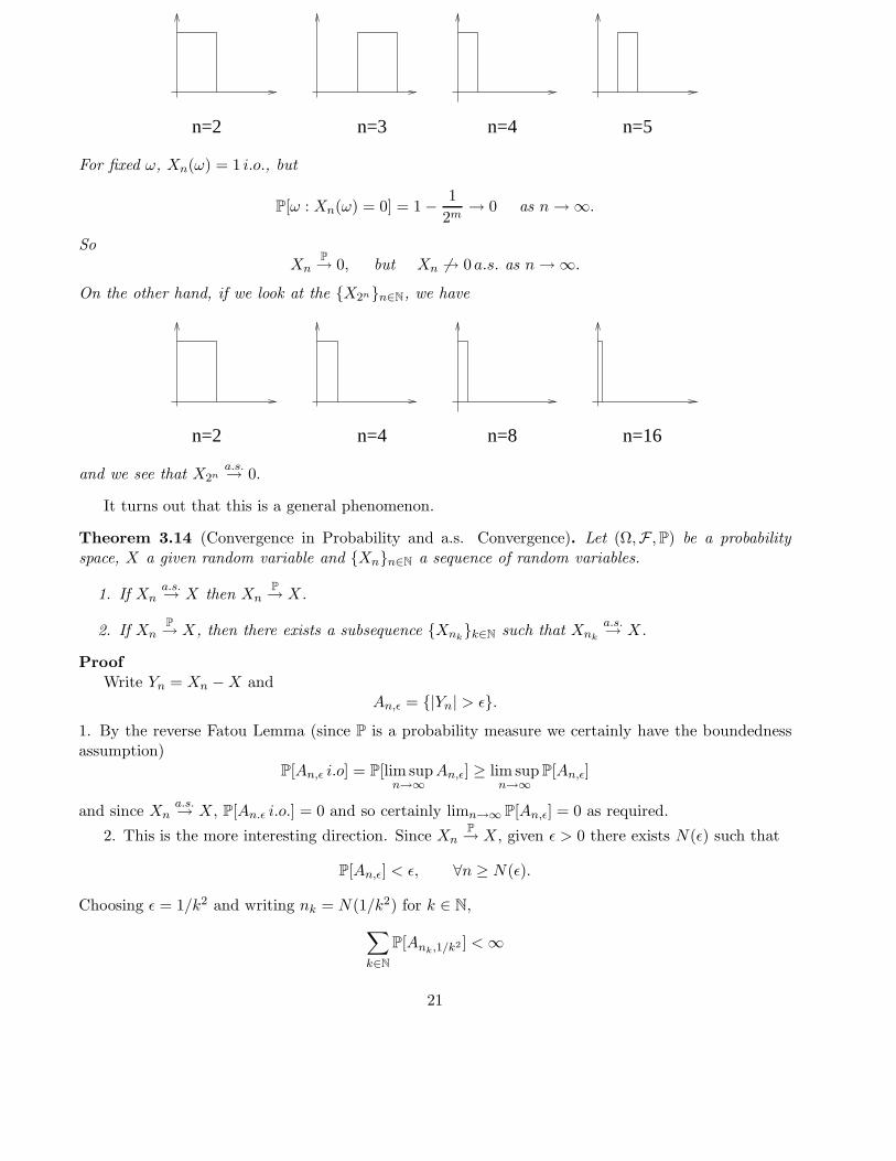
Example 3.13 (Convergence in probability does not imply a.s. convergence). To understand what’sgoing on in (9) and (10), let’s stick with [0, 1] with the Borel sets and Lebesgue measure as our probabilityspace. We define Xnn∈N as follows:

for each n there is a unique pair of integers (m,k) such that n = 2m + k. We set

Xn(ω) = 1[2−mk,2−m(k+1))(ω).

Pictorially we have a ‘moving blip’ which travels repeatedly across [0, 1] getting narrower at each pass.

20

n=5n=2 n=3 n=4

For fixed ω, Xn(ω) = 1 i.o., but

P[ω : Xn(ω) = 0] = 1 − 1

2m→ 0 as n → ∞.

SoXn

P→ 0, but Xn 6→ 0 a.s. as n → ∞.

On the other hand, if we look at the X2nn∈N, we have

n=16n=2 n=4 n=8

and we see that X2na.s.→ 0.

It turns out that this is a general phenomenon.

Theorem 3.14 (Convergence in Probability and a.s. Convergence). Let (Ω,F , P) be a probabilityspace, X a given random variable and Xnn∈N a sequence of random variables.

1. If Xna.s.→ X then Xn

P→ X.

2. If XnP→ X, then there exists a subsequence Xnk

k∈N such that Xnk

a.s.→ X.

Proof

Write Yn = Xn − X andAn,ǫ = |Yn| > ǫ.

1. By the reverse Fatou Lemma (since P is a probability measure we certainly have the boundednessassumption)

P[An,ǫ i.o] = P[lim supn→∞

An,ǫ] ≥ lim supn→∞

P[An,ǫ]

and since Xna.s.→ X, P[An.ǫ i.o.] = 0 and so certainly limn→∞ P[An,ǫ] = 0 as required.

2. This is the more interesting direction. Since XnP→ X, given ǫ > 0 there exists N(ǫ) such that

P[An,ǫ] < ǫ, ∀n ≥ N(ǫ).

Choosing ǫ = 1/k2 and writing nk = N(1/k2) for k ∈ N,

∑

k∈N

P[Ank,1/k2 ] < ∞

21

and so by BC1, P[Ank,1/k2 i.o.] = 0. That is

P[lim supn→∞

Ank,1/k2 ] = 0

which, in turn, says Xnk

a.s.→ X as required. 2

The First Borel-Cantelli Lemma provides a very powerful tool for proving almost sure convergenceof a sequence of random variables. It’s successful application often rests on being able to find goodbounds on the random variables Xnn∈N. We end this section with some inequalities that are oftenhelpful in this context. The first is trivial, but has many applications.

Lemma 3.15 (Chebyshev’s inequality). Let (Ω,F , P) be a probability space and X a non-negativerandom variable, then for each λ > 0

P[X ≥ λ] ≤ 1

λE[X].

More generally, let Y be any random variable (not necessarily non-negative) and let φ : R → [0,∞] benon-decreasing and measurable. Then for any λ ∈ R,

P[Y ≥ λ] = P[φ(Y ) ≥ φ(λ)]

≤ 1

φ(λ)E[φ(Y )].

The second inequality is often applied with φ(x) = eθx to obtain

P[Y ≥ λ] ≤ e−θλE[eθY ]

and then optimised over θ.For the next inequality we recall

Definition 3.16 (Convex function). Let I ⊆ R be an interval. A function c : I → R is convex if forall x, y ∈ I and t ∈ [0, 1],

c (tx + (1 − t)y) ≤ tc(x) + (1 − t)c(y).

Theorem 3.17 (Jensen’s inequality). Suppose that (Ω,F , P) is a probability space and X an integrablerandom variable taking values in I. Let c : I → R be convex. Then

E[c(X)] ≥ c (E[X]) .

Important examples of convex functions include x2, ex, 1/x. To check that a twice continuouslydifferentiable function is convex, it suffices to check that c′′(x) > 0 for all x.

The proof of Theorem 3.17 rests on the following lemma.

Lemma 3.18. Suppose that c : I → R is convex and let m be an interior point of I. Then there exitsa, b ∈ R such that c(x) ≥ ax + b for all x with equality at x = m.

Proof

For x < m < y, by convexity,

c(m) ≤ (m − x)

(y − x)c(y) +

(y − m)

(y − x)c(x).

22

Rearranging,c(m) − c(x)

m − x≤ c(y) − c(m)

y − m.

So for an interior point m, since the left hand side does not depend on y and the right hand side doesnot depend on x,

supx<m

c(m) − c(x)

m − x≤ inf

y>m

c(y) − c(m)

y − m

and choosing a so that

supx<m

c(m) − c(x)

m − x≤ a ≤ inf

y>m

c(y) − c(m)

y − m

we have that c(x) ≥ c(m) + a(x − m) for all x ∈ I. 2

Proof of Theorem 3.17

Since E[X] is certainly an interior point of I (other than in the trivial case X is almost surelyconstant), set m = E[X] in the previous lemma and we have

c(X) ≥ c (E[X]) + a(X − E[X]).

Now take expectations to recoverE[c(X)] ≥ c (E[X])

as required. 2

4 Conditional Expectation

Probability is a measure of ignorance. When new information decreases that ignorance we change ourprobabilities. We formalised this in mods through Bayes’ rule. For a probability space (Ω,F , P) andA,B ∈ F

P[A|B] =P[A ∩ B]

P[B].

We want now to introduce an extension of this which lies at the heart of martingale theory: the notionof conditional expectation. First a preliminary definition:

Definition 4.1 (Equivalence class of a random variable). Let (Ω,F , P) be a probability space and X arandom variable. The equivalence class of X is the collection of random variables that differ from Xonly on a null set.

Definition 4.2 (Conditional Expectation). Let (Ω,F , P) be a probability space and let X be an in-tegrable random variable (that is one for which E[|X|] < ∞). Let G be a sub σ-algebra of F . Theconditional expectation E[X|G] is any G-measurable, integrable random variable Z in the equivalenceclass of random variables such that

∫

ΛZdP =

∫

ΛXdP for any Λ ∈ G.

The integrals of X and Z over sets Λ ∈ G are the same, but X is F-measurable whereas Z isG-measurable. The conditional expectation satisfies

∫

ΛE[X|G]dP =

∫

ΛXdP for any Λ ∈ G (11)

23

and we shall call (11) the defining relation.Just as probability of an event is a special case of expectation (corresponding to integrating an

indicator function rather than a general measurable function), so conditional probability is a specialcase of conditional expectation. In that case (11) becomes

∫

ΛP[A|G]dP = P[A ∩ Λ] for any Λ ∈ G. (12)

Let’s see how this fits with our understanding from mods. Suppose that X is a discrete random variabletaking values xnn∈N. Then the events X = xn are a partition of Ω (that is Ω is a disjoint unionof these events.) So, by the Partition Theorem of mods,

P[A] = P

[⋃

n∈N

(A ∩ X = xn)]

=∑

n∈N

P[A ∩ X = xn]

=∑

n∈N

P[A|X = xn]P[X = xn].

Now we ‘randomize’ - replace P[X = xn] by 1X=xn and we write

P[A|X] = P[A|σ(X)] =

∞∑

n=1

P[A|X = xn]1X=xn,

which means that for a given ω ∈ Ω

P[A|σ(X)] =

P[A|X = x1], if X(ω) = x1,P[A|X = x2], if X(ω) = x2,

· · · · · ·P[A|X = xn], if X(ω) = xn.

To see that this coincides with (12), notice that if Λ ∈ σ(X) then it can be expressed as a union ofsets of the form X = xn (the advantage with working with discrete random variables again - theσ-algebra is easy) and for such Λ

∫

Λ

(∞∑

n=1

P[A|X = xn]1X=xn

)dP =

∑

n:xn∈Λ

P[A|X = xn]P[X = xn]

=∑

n:xn∈Λ

P[A ∩ X = xn]

= P[A ∩ Λ].

This would have worked equally well for any other partition in place of X = xnn∈N. So moregenerally, let Λnn∈N be a partition of Ω and let E[X|Λn] be the conditional expectation relative tothe conditional measure P[·|Λn] so that

E[X|Λn] =

∫

ΩX(ω)dP[ω|Λn] =

∫Λn

XdP

P[Λn].

24

Then for Λ =∑

j∈J Λj ∈ G we obtain (using the disjointness of the Λj ’s)

∫

Λ

(∞∑

n=1

E[X|Λn]1Λn

)dP =

∑

j∈J

∞∑

n=1

∫

Λj

E[X|Λn]1Λn1ΛjdP (the summand is zero if n 6= j)

=∑

j∈J

∫

Λj

E[X|Λj ]dP

=∑

j∈J

E[X|Λj ]P[Λj]

=∑

j∈J

∫Λj

XdP

P[Λj ]P[Λj ]

=∑

j∈J

∫

Λj

XdP

=

∫

∪jΛj

XdP =

∫

ΛXdP.

So in this case

E[X|G] =

∞∑

n=1

E[X|Λn]1Λn a.s.,

or, spelled out, that

E[X|G] =

E[X|Λ1] if ω ∈ Λ1,E[X|Λ2] if ω ∈ Λ2,

· · · · · ·E[X|Λn] if ω ∈ Λn,

· · · · · ·So E[X|G] is constant on each set Λi (where it takes the value E[X|Λi]).

So far we have proved that conditional expectations exist for sub σ-algebras G generated by parti-tions. Before proving existence in the general case we show that we have (a.s.) uniqueness.

Proposition 4.3 (Almost sure uniqueness of conditional expectation). Let (Ω,F , P) be a probabilityspace, X an integrable random variable and G a sub σ-algebra of F . If Y and Z are two G-measurablerandom variables that both satisfy the defining relation (11), then P[Y 6= Z] = 0. That is Y and Zagree up to a null set.

Proof

Since Y and Z are both G-measurable,

Λ1 = ω : Y (ω) < Z(ω) ∈ G,

so using the defining relation ∫

Λ1

(Y − Z)dP = 0

which implies P[Λ1] = 0.Similarly,

Λ2 = ω : Y (ω) > Z(ω) ∈ G

25

and ∫

Λ2

(Y − Z)dP = 0

gives P[Λ2] = 0 which completes the proof. 2

For existence in the general case we will use another important result from measure theory. Firsta definition.

Definition 4.4. Let (Ω,F , P) be a probability space and let Q be a finite measure on (Ω,F). Themeasure Q is absolutely continuous with respect to P iff

P[a] = 0 =⇒ Q[A] = 0 ∀A ∈ F .

We write Q ≪ P.

Theorem 4.5 (The Radon-Nikodym Theorem). Let (Ω,F , P) be a probability space and suppose thatQ is a finite measure that is absolutely continuous with respect to P. Then there exists an F-measurablerandom variable Z with finite mean such that

Q[A] =

∫

AZdP for all A ∈ F .

Moreover, Z is P-a.s. unique. It is written

Z =dQ

dP

and is called the Radon-Nikodym derivative of Q with respect to P.

Theorem 4.6 (Existence of conditional expectation). Let (Ω,F , P) be a probability space, X an in-tegrable random variable and G a sub σ-algebra of F . Then there exists a unique equivalence class ofrandom variables with are measurable with respect to G and for which the defining relation (11) holds.

Proof

Let P|G denote the measure P restricted to the sub σ-algebra G. Set

Q[A] =

∫

AXdP for A ∈ G.

Then Q ≪ P|G and so the Radon-Nikodym Theorem applies to Q, P|G on (Ω,G). Write

E[X|G] =dQ

dP|G.

2

It is much harder to write out E[X|G] explicitly when G is not generated by a partition. But notethat if G = σ(Y ) for some random variable Y on (Ω,F , P), then any G-measurable function can, inprinciple, be written as a function of Y . We saw an example of this with our branching process in §0.2.If Zn was the number of descendants of a single ancestor after n generations, then

E[Zn+1|σ(Zn)] = µZn

where µ is the expected number of offspring of a single individual.In general, of course, the relationship can be much more complicated.

26

Exercise 4.7. Roll a fair die until we get a six. Let Y be the total number of rolls and X the numberof 1’s. Show that

E[X|Y ] =1

5(Y − 1) and E[X2|Y ] =

1

25(Y 2 + 2Y − 3).

Let’s turn to some elementary properties of conditional expectation. Most of the following areobvious. Always remember that whereas expectation is a number, conditional expectation is a functionon (Ω,G) and, since conditional expectation is only defined up to equivalence (so up to null sets) wehave to qualify many of our statements with the caveat ‘a.s.’.

Proposition 4.8. Let (Ω,F , P) be a probability space, X and Y integrable random variables, G ⊆ F asub σ-algebra and a, b, c real numbers. Then

1. E[E[X|G]] = E[X].

2. E[aX + bY |G]a.s.= aE[X|G] + bE[Y |G].

3. If X is G-measurable, then E[X|G]a.s.= X.

4. E[c|G]a.s.= c.

5. E[X|∅,Ω] = E[X].

6. If X ≤ Y a.s. then E[X|G] ≤ E[Y |G] a.s.

7. |E[X|G]| ≤ E[|X||G].

8. If X is independent of G then E[X|G] = E[X] a.s.

Proof

The proofs all follow from the requirement that E[X|G] be G-measurable and the defining rela-tion (11). We just do some examples.

1. Set Λ = R in the defining relation.2. ∫

ΛE[aX + bY |G]dP =

∫

Λ(aX + bY )dP

= a

∫

ΛXdP + b

∫

ΛY dP (linearity of the integral)

= a

∫

ΛE[X|G]dP + b

∫

ΛE[Y |G]dP

=

∫

Λ(aE[X|G] + bE[Y |G])dP,

where the last line again follows by linearity of the integral. And if two G-measurable functions agreeon integration over any G-measurable set then they are P-a.s equal.

5. The sub σ-algebra is just ∅,Ω and so E[X|∅,Ω] (in order to be measurable with respect to∅,Ω) must be constant. Now integrate over Ω to identify that constant.

Jumping to 8. Note that E[X] is G-measurable and for Λ ∈ G∫

ΛE[X]dP = E[X]P[Λ] = E[X]E[1Λ]

= E[X1Λ] (by independence)

=

∫X1ΛdP =

∫

ΛXdP,

27

so the defining relation holds. 2

Notice that 8 is intuitively clear. If X is independent of G, then telling me about events in G tellsme nothing about X and so my assessment of its expectation does not change. On the other hand for3, if X is G-measurable, then telling me about events in G actually tells me the value of X.

The conditional counterparts of our convergence theorems of integration also hold good.

Proposition 4.9 (Conditional Convergence Theorems). Let (Ω,F , P) be a probability space, Xnn∈N

a sequence of integrable random variables, X a random variable and G a sub σ-algebra of F .

1. cMON: If Xn ↑ X as n → ∞, then E[Xn|G] ↑ E[X|G] a.s. as n → ∞.

2. cFatou: If Xnn∈N are non-negative then

E[lim infn→∞

Xn|G] ≤ lim infn→∞

E[Xn|G] a.s.

3. If Xnn∈N are non-negative and Xn ≤ Z for all n where Z is an integrable random variable then

E[lim supn→∞

Xn|G] ≥ lim supn→∞

E[Xn|G] a.s.

4. cDOM: If Y is an integrable random variable and |Xn| ≤ Y for all n and Xna.s.→ X then

E[Xn|G]a.s.→ E[X|G] as n → ∞.

The proofs all use the defining relation (11) to transfer statements about convergence of the condi-tional probabilities to our usual convergence theorems and are left as an exercise.

The following two results are incredibly useful in manipulating conditional expectations. The firstis sometimes referred to as ‘taking out what is known’.

Proposition 4.10. Let (Ω,F , P) be a probability space and X, Y integrable random variables. Let Gbe a sub σ-algebra of F and suppose that Y is G-measurable. Then

E[XY |G]a.s.= Y E[X|G].

Proof

We use the ‘standard machine’.First suppose that X and Y are non-negative. If Y = 1A for some A ∈ G, then for any Λ ∈ G we

have Λ ∩ A ∈ G and so by the defining relation (11)∫

ΛY E[X|G]dP =

∫

Λ∩AE[X|G]dP =

∫

Λ∩AXdP =

∫

ΛY XdP.

Now extend by linearity to simple random variables Y . Next if Ynn≥1 are simple random variableswith Yn ↑ Y as n → ∞, it follows that YnX ↑ Y X and YnE[X|G] ↑ Y E[X|G] from which we deduce theresult by the MCT. Finally, for X, Y not necessarily non-negative, write XY = (X+ −X−)(Y + −Y −)and use linearity of the integral. 2

Proposition 4.11 (Tower property of conditional expectations). Let (Ω,F , P) be a probability spaceand X an integrable random variable and F1, F2 sub σ-algebras of F with F1 ⊆ F2. Then

E [E[X|F2]| F1] = E[X|F1] a.s.

In other words, writing Xi = E[X|Fi],

X1 = E[X2|F1] a.s.

28

This extends Part 5 of Proposition 4.8 which dealt with the case F1 = ∅,Ω.The usefulness of this result mirrors that of the ‘partition theorem’ of mods probability theory. If

sets A1, . . . , An partition Ω then for any random variable X,

E[X] =

n∑

i=1

E[X|Ai]P[Ai].

Proof of Proposition 4.11

Choose Λ ∈ F1 and observe that automatically Λ ∈ F2. Applying the defining relation (three times)gives ∫

ΛE [E[X|F2]| F1] dP =

∫

ΛE[X|F2]dP =

∫

ΛXdP =

∫

ΛE[X|F1]dP.

2

Jensen’s inequality also extends to the conditional case.

Proposition 4.12 (Conditional Jensen’s Inequality). Suppose that (Ω,F , P) is a probability space andthat X is an integrable random variable taking values in an open interval I ⊆ R. Let c : I → R beconvex and let G be a sub σ-algebra of F . If E[|c(X)|] < ∞ then

E[c(X)|G] ≥ c (E[X|G]) a.s.

Proof

Recall from our proof of Jensen’s inequality that if c is convex, then for x < m < y ∈ I

c(m) − c(x)

m − x≤ c(y) − c(m)

y − m. (13)

Letting x ↑ m and writing

(D−c)(q) = limr↑q

c(q) − c(r)

q − r

for the left derivative of c at the point q, we see that

c(y) ≥ supm∈I

(D−c)(m)(y − m) + c(m)

and in fact we have equality (by setting y = m on the right hand side).(Existence of (D−(c) follows from (13) which also automatically guarantees continuity of c).In particular, there exists a pair of sequences ann∈N, bnn∈N of real numbers such that

c(x) = supnanx + bn for x ∈ I.

Now for our random variable X, since c(X) ≥ anX + bn we have

E[c(X)|G] ≥ anE[X|G] + bn a.s. (14)

Since the union of a countable union of null sets is null (Part A Integration) we can arrange for (14)to hold simultaneously for all n ∈ N except possibly on a null set and so

E[c(X)|G] ≥ supnanE[X|G] + bn a.s.

= c (E[X|G]) a.s.

2

An important special case is c(x) = xp for p > 1. In particular, for p = 2

E[X2|G] ≥ E[X|G]2.

This leads to another interesting characteristaion of E[X|G].

29

Remark 4.13 (Conditional Expectation and Mean Square Approximation). Let (Ω,F , P) be a proba-bility space and X, Y square integrable random variables. Let G be a sub σ-algebra of F and supposethat Y is G-measurable. Then

E[(Y − X)2] = E[Y − E[X|G] + E[X|G] − X2

]

= E[(Y − E[X|G])2] + E[(E[X|G] − X)2] + 2E[(Y − E[X|G])(E[X|G] − X)].

Now Y is G-measurable and so, using Proposition 4.8 part 1 and Proposition 4.10 we have

E[(Y − E[X|G])(E[X|G] − X)] = E [E[(Y − E[X|G])(E[X|G] − X)|G]

= E [(Y − E[X|G]) (E[E[X|G] − X|G])] = 0,

and so the cross-terms vanish.In particular, we can minimise E[(Y − X)2] by choosing Y = E[X|G]. In other words, E[X|G] is

the best mean-square approximation of X among all G-measurable random variables.If you have already done Hilbert space theory then E[X|G] is the orthogonal projection of X ∈

L2(Ω,F , P) onto the closed subspace L2(Ω,G, P). Indeed this is a route to showing that conditionalexpectations exist without recourse to the Radon-Nikodym Theorem.

We are now, finally, in a position to introduce martingales.

5 Martingales

Much of modern probability theory derived from two sources: the mathematics of measure and gam-bling. (The latter perhaps explains why it took so long for probability theory to become a respectablepart of mathematics.) Although the term ‘martingales’ has many meanings outside mathematics - itis the name given to a strap attached to a fencer’s epee, it’s a strut under the bowsprit of a sailingship and it is part of a horse’s harness that prevents the horse from throwing its head back - it’sintroduction to mathematics, by Ville in 1939, was inspired by the gambling strategy ‘the infalliblemartingale’. This is a strategy for making a sure profit on games such as roulette in which one makesa sequence of independent bets. The strategy is to stake £1 (on, say, a specific number at roulette)and keep doubling the stake until that number wins. When it does, all previous losses and more arerecouped and you leave the table with a profit. It doesn’t matter how unfavourable the odds are, onlythat a winning play comes up eventually. But the martingale is not infallible. Nailing down why inpurely mathematical terms had to await the development of martingales in the mathematical sense byJ.L. Doob in the 1940’s. Doob originally called them ‘processes with property E’, but in his famousbook on stochastic processes he reverted to the term ‘martingale’ and he later attributed much of thesuccess of martingale theory to the name.

The mathematical term martingale doesn’t refer to the gambling strategy, but rather models theoutcomes of a series of fair games (although as we shall see this is only one application).

We begin with some terminology.

Definition 5.1 (Filtration). A filtration on the probability space (Ω,F , P) is a sequence Fnn≥0 ofsub σ-algebras such that for all n, Fn ⊆ Fn+1.

Usually n is interpreted as time and Fn represents knowledge accumulated by time n (we neverforget anything).

Definition 5.2 (Adapted stochastic process). A stochastic process, Xnn≥0 is a collection of randomvariables defined on some probability space (Ω,F , P).

We say that Xnn≥0 is adapted to the filtration Fnn≥0 if, for each n, Xn is Fn-measurable.

30

Definition 5.3 (Martingale, submartingales, supermartingale). Let (Ω,FP) be a probability space andFnn≥0 a filtration. An integrable, Fn-adapted stochastic process Xnn≥0 is called

1. a martingale if E[Xn+1|Fn] = Xn a.s. for n ≥ 0,

2. a submartingale if E[Xn+1|Fn] ≥ Xn a.s. for n ≥ 0,

3. a supermartingale if E[Xn+1|Fn] ≤ Xn a.s. for n ≥ 0.

If we think of Xn as our accumulated fortune when we make a sequence of bets, then a martingalerepresents a fair game in the sense that the conditional expectation of Xn+1−Xn, given our knowledgeat the time when we make the (n + 1)st bet (that is Fn), is zero. A submartingale represents afavourable game and a supermartingale an unfavourable game.

Note that the concept of martingale makes no sense unless we specify the filtration. Very often, ifa filtration is not specified, it is implicitly assumed that the natural filtration is intended.

Definition 5.4 (Natural filtration). The natural filtration associated with a stochastic process Xnn≥0

on the probability space (Ω,F , P) is defined by

Fn = σ(X0,X1, . . . ,Xn), n ≥ 0.

A stochastic process is automatically adapted to the natural filtration associated with it.Here are some elementary properties.

Proposition 5.5. Let (Ω,F , P) be a probability space.

1. A stochastic process Xnn≥0 on (Ω,F , P) is a submartingale w.r.t. the filtration Fnn≥0 if andonly if −Xnn≥0 is a supermartingale. It is a martingale if and only if it is both a martinagleand a submartingale.

2. If Xnn≥0 is a martingale w.r.t. Fnn≥0 then

E[Xn] = E[X0] for all n.

If Xnn≥0 is a submartingale and m < n then

Xm ≤ E[Xn|Fm] a.s.

andE[Xm] ≤ E[Xn].

If Xnn≥0 is a supermartingale and m < n then

Xm ≥ E[Xn|Fm] a.s.

andE[Xm] ≥ E[Xn].

3. If Xnn≥0 is a submartingale w.r.t. some filtration Fnn≥0, then it is also a submartingalewith respect to the natural filtration Gn = σ(X0, . . . ,Xn).

31

Proof

1 is obvious.2. We prove the result when Xnn≥0 is a submartingale w.r.t Fnn≥0.The result is true for n = m+1 by definition. Suppose that it is true for n = m+k for some k ∈ N.

ThenXm+k ≤ E[Xm+k+1|Fm+k]

(by definition) and so (by the inductive hypothesis)

Xm ≤ E [E[Xm+k+1|Fm+k]| Fm]

and since Fm ⊆ Fm+k, the tower property gives

Xm ≤ E[Xm+k+1|Fm]i a.s.

and the result follows by induction. For the second conclusion, take expectations.3. Xnn≥0 is adapted to its natural filtration Gnn≥0 and since (by definition) Gn is the smallest

σ-algebra with respect to which X0, . . . ,Xn are all measurable, Gn ⊆ Fn. Thus, by the towerproperty,

E[Xn|Gm] = E [E[Xn|Fm]| Gm] ≥ E[Xm|Gm] = Xm.

2

Proposition 5.6. Let (Ω,F , P) be a probability space. Suppose that Xnn≥0 is a martingale withrespect to the filtration Fnn≥0. Let c be a convex function on R. If c(Xn) is an integrable randomvariable for each n ≥ 0, then c(Xn)n≥0 is a submartingale w.r.t Fnn≥0.

Proof

By Jensen’s inequality for conditional expectations

c(Xm) = c (E[Xn|Fm]) (martingale property)

≤ E[c(Xn)|Fm] (Jensen’s inequality).

2

Corollary 5.7. If Xnn≥0 is a martingale w.r.t. Fnn≥0 then (subject to integrability) |Xn|n≥0,X2

nn≥0, eXnn≥0, e−Xnn≥0, max(Xn,K)n≥0 are all submartingales w.r.t. Fnn≥0.

Example 5.8 (Sums of independent random variables). Suppose that Y1, Y2, . . . are independent ran-dom variables on the probability space (Ω,F , P) and that E[Yn] = 0 for each n. Define

Xn =

n∑

k=1

Yk, X0 = 0.

Then Xnn≥0 is a martingale with respect to the natural σ-algebra

Fn = σ(X1, . . . ,Xn) = σ(Y1, . . . , Yn).

In this sense martingales generalise the notion of sums of independent random variables with meanzero. The independent random variables Yii∈N of Example 5.8 can be replaced by martingale differ-ences (which are not necessarily independent).

32

Definition 5.9 (Martingale differences). Let (Ω,F , P) be a probability space and Fnn≥0 a filtra-tion. A sequence Unn∈N of integrable random variables, adapted to the filtration Fnn∈N is called amartingale difference sequence if

E[Un+1|Fn] = 0 a.s. for all n ≥ 0.

Example 5.10. Let (Ω,F , P) be a probability space and let Xnn∈N be a sequence of independent,non-negative random variables with E[Xn] = 1 for all n. Define

M0 = 1, Mn =

n∏

i=1

Xi for n ≥ 1.

Let Fnn∈N be the natural filtration associated with Mnn∈N. Then Mnn∈N is a martingale. (Ex-ercise).

This is an example where the martingale is (obviously) not a sum of independent random variables.

Example 5.11. Let (Ω,F , P) be a probability space and let Fnn∈N be a filtration. Let X be anintegrable random variable (that is E[|X|] < ∞). Then setting

Xn = E[X|Fn], n ≥ 1,

Xnn∈N is a martingale w.r.t. Fnn∈N. This is an easy consequence of the tower property. Indeed

E[Xn+1|Fn] = E[E[X|Fn+1]|Fn] = E[X|Fn] a.s.

We shall see later that a large class of martingales (called uniformly integrable) can be written in thisway. One can think of Fnn∈N as representing unfolding information about X and we’ll see thatXn → X a.s. as n → ∞.

Definition 5.12 (Predictable process). Let (Ω,F , P) be a probability space and Fnn∈N a filtration.A sequence Unn∈N of random variables is predictable with respect to Fnn∈N if Un is measurablewith respect to Fn−1 for all n ≥ 1.

Example 5.13 (Discrete stochastic integral or martingale transform). Let (Ω,F , P) be a probabilityspace and Fnn∈N a filtration. Let Ynn∈N be a martingale with difference sequence Unn≥1. Supposethat vnn≥1 is a predictable sequence. Set

X0 = 0, Xn =n∑

k=1

Ukvk for n ≥ 1.

The sequence Xnn≥1 is called a martingale transform and is itself a martingale. It is a discreteversion of the stochastic integral. To check the martingale property:

E[Xn+1|Fn] = E

[n∑

k=1

Ukvk|Fn

]+ E[Un+1vn+1|Fn]

= Xn + vn+1E[Un+1|Fn] (using Proposition 4.10)

= Xn.

33

Typical examples of predictable sequences appear in gambling or finance contexts where they mightconstitute strategies for future action. The strategy is then based on the current state of affairs. If, forexample, (k − 1) rounds of some gambling game have just been completed, then the strategy for thekth round is vk ∈ Fk−1. The change in fortune in the kth round is then Ukvk.

Another situation is when vk = 1 as long as some special event has not yet happened and vk = 0thereafter. That is the game goes on until the event occurs. This is called a stopped martingale - atopic we’ll return to in due course.

There are more examples on the problem sheet. Here is one last one.

Example 5.14. Let Yii∈N be independent random variables such that E[Yi] = µi, var(Yi) = E[Y 2i ]−

E[Yi]2 = σ2

i . Let

s2n =

n∑

i=1

σ2i , n ≥ 1.

(That is s2n = var(

∑ni=1 Yi) by independence.) Take Fnn∈N to be the natural filtration generated by

Ynn∈N.It is easy to check that

Xn =n∑

i=1

(Yi − µi)

is a martingale (just by modifying Example 5.8) and so by Proposition 5.6, since c(x) = x2 is a convexfunctions, X2

nn∈N is a submartingale. But we can recover a martingale from it by compensation:

Mn =

(n∑

i=1

(Yi − µi)

)2

− s2n, n ≥ 1

is a martingale with respect to Fnn≥1.

Proof

By considering the sequence Yi = Yi − µi of independent mean zero random variables if necessary,we see that w.l.o.g. we may assume µi = 0 for all i. Then

E[Mn+1|Fn] = E

(

n∑

i=1

Yi + Yn+1

)2

− s2n+1

∣∣∣∣∣∣Fn

= E

(

n∑

i=1

Yi

)2

+ 2Yn+1

n∑

i=1

Yi + Y 2n+1 − s2

n+1|Fn

=

(n∑

i=1

Yi

)2

+ 2

n∑

i=1

YiE[Yn+1|Fn] + E[Y 2n+1|Fn] − s2

n − σ2n+1 a.s.

= Mn

since E[Yn+1|Fn] = 0 and E[Y 2n+1|Fn+1] = σ2

n+1. 2

This process of ‘compensation’, whereby we correct a process by something predictable (in thisexample it was deterministic) in order to obtain a martingale reflects a general result due to Doob.

Theorem 5.15 (Doob’s Decomposition Theorem). Let (Ω,F , P) be a probability space and Fnn∈N afiltration. Let Xnn∈N be a sequence of integrable random variables, adapted to Fnn∈N. Then

34

1. Xnn∈N has a Doob decomposition

Xn = X0 + Mn + An (15)

where Mnn∈N is a martingale and Ann∈N is a predictable process and M0 = 0 = A0. More-

over, if Xn = X0 + Mn + An is another Doob decompositon of Xnn∈N then

P[Mn = Mn, An = An for all n] = 1.

2. Xnn∈N is a supermartingale if and only if Ann∈N in (15) is a decreasing process and asubmartingale if and only if Ann∈N is an increasing process.

Proof

Let

Mn =

n∑

k=1

(Xk − E[Xk|Fk−1]) , and An = Xn − Mn, n ≥ 1.

Then, sinceE[Xk − E[Xk|Fk−1]|Fk−1] = 0,

the process Mnn∈N is a martingale. We must check that Ann∈N is predictable. But

An = Xn −n∑

k=1

(Xk − E[Xk|Fk−1]) =n∑

k=1

E[Xk|Fk−1] −n−1∑

k=1

Xk

which is Fn−1-measurable.That establishes existence of a decomposition. For uniqueness, suppose that Xn = X0 + Mn + An.

Then by predictability,

An+1 − An = E[An+1 − An|Fn]

= E[(Xn=1 − Xn) − (Mn+1 − Mn)|Fn]

= E[Xn+1|Fn] − Xn

= An+1 − An,

which combined with A0 = 0 = A0 proves uniqueness of the increasing process and therefore, since

Mn = Xn − X0 − An = Xn − X0 − An = Mn,

also proves uniqueness of the martingale.2 is obvious. 2

Remark 5.16 (The angle bracket process 〈M〉). Let (Ω,F , P) be a probability space, Fnn∈N a fil-tration and Mnn∈N a martingale with respect to Fnn∈N with E[M2

n] < ∞ for each n. (Such amartingale is called an L2-martingale.) Then by Proposition 5.6, M2

nn∈N is a submartingale. Thusby Theorem 5.15 it has a Doob decomposition (which is essentially unique),

M2n = Nn + An

where Nnn∈N is a martingale and Ann∈N is an increasing predictable process. The process Ann∈N

is often denoted by 〈M〉nn∈N.Note that E[M2

n] = E[An] and that

An − An−1 = E[(Mn − Mn−1)2|Fn−1].

It turns out that 〈M〉nn∈N is an extremely powerful tool with which to study Mnn∈N. It is beyondour scope here, but see for example Neveu 1975, Discrete Parameter Martingales.

35

6 Stopping Times and Stopping Theorems

Much of the power of martingale methods, as we shall see, comes from the fact that (under suitableboundedness assumptions) the martingale property is preserved if we ‘stop’ the process at certainrandom times. Such times are called ‘stopping times’ (or sometimes ‘optional times’).

Intuitively, stopping times are times that we can recognise when they arrive, like the first timeheads comes up in a series of coin tosses or the first time the FTSE 100 index takes a 3% fall in a singleday. They are times which can be recognised without reference to the future. Something like ‘the dayin December when the FTSE 100 reaches its maximum’ is not a stopping time - we must wait until theend of December to determine the maximum, and by then, in general, the time has passed.

Stopping times can be used for strategies of investing and other forms of gambling. We recognisethem when they arrive and can make decisions based on them (for example to stop playing).

Definition 6.1 (Stopping time). Let (Ω,F , P) be a probability space and Fnn∈N a filtration. Apositive integer-valued (possibly infinite) random variable τ is called a stopping time with respect toFnn∈N if τ = n ∈ Fn for all n or, equivalently, if τ > n ∈ Fn for all n. Stopping times aresometimes called optional times.

Warning: Some authors assume P[τ < ∞] = 1.

Lemma 6.2. Let (Ω,F , P) be a probability space, Fnn∈N a filtration, Mnn∈N a martingale with re-spect to Fnn∈N and τ a stopping time with respect to Fnn∈N. Then Mn∧τn∈N is also a martingalewith respect to Fnn∈N.

Proof

Take vn = 1τ>n−1 in Example 5.13. 2

This Lemma tells us that E[Mn∧τ ] = E[M0], but can we let n → ∞ to obtain E[Mτ ] = E[M0]? Theanswer is ‘no’.

Example 6.3. Let Yii∈N be i.i.d. random variables with P[Yi = 1] = P[Yi = −1] = 1/2. SetXn =

∑nk=1 Yk, n ≥ 1. That is Xn is the position of a simple random walk started from the origin

after n steps. In particular, Xnn∈N is a martingale and so E[Xn] = 0 for all n.Now let τ = minn : Xn = 1. It is clear that τ is a stopping time and evidently Xτ = 1. But then

E[Xτ ] = 1 6= 0 = E[X0].

The problem is that τ is too large - E[τ ] = ∞. It turns out that if we impose suitable boundednessassumptions then we will have E[Mτ ] = E[M0] and that is the celebrated Optional Stopping Theorem.There are many variants of this result.

Theorem 6.4 (Doob’s Optional Stopping Theorem). Let (Ω,F , P) be a probability space, Fnn∈N

a filtration, Mnn∈N a martingale with respect to Fnn∈N and τ a stopping time with respect toFnn∈N. Then Mτ is integrable and

E[Mτ ] = E[M0] (16)

in each of the following situations:

1. τ is a.s. finite and Mnn∈N is bounded (that is there exists K such that |Mn(ω)| ≤ K for everyn ∈ N and every ω ∈ Ω).

2. τ is bounded (for some N ∈ N, τ(ω) ≤ N for all ω ∈ Ω).

3. E[τ ] < ∞ and there exists M < ∞ such that

E [ |Mn+1 − Mn|| Fn] < M, for all n.

36

Proof

1. Because τ < ∞, limn→∞ Mn∧τ = Mτ a.s. and since Mnn∈N is bounded we may apply theBounded Convergence Theorem (that is the DCT with dominating function g(ω) ≡ K) to deduce theresult.

2. Take n = N in Lemma 6.2.3. Note first that setting M0∧τ = 0,

|Mn∧τ | =

∣∣∣∣∣

n∑

i=1

(Mi∧τ − M(i−1)∧τ )

∣∣∣∣∣

≤n∑

i=1

|Mi∧τ − M(i−1)∧τ |

≤∞∑

i=1

1τ≥i|Mi∧τ − M(i−1)∧τ |. (17)

Now

E

[∞∑

i=1

1τ≥i|Mi∧τ − M(i−1)∧τ |]

=

∞∑

i=1

E[1τ≥i|Mi∧τ − M(i−1)∧τ |] (by MCT)

=∞∑

i=1

E[E[1τ≥i|Mi∧τ − M(i−1)∧τ |

∣∣Fi−1]]

(tower property)

=∞∑

i=1

E[1τ≥iE[ |Mi∧τ − M(i−1)∧τ |

∣∣Fi−1]]

(since τ ≥ i ∈ Fi−1)

≤ M

∞∑

i=1

E[1τ≥i]

= M

∞∑

i=1

P[τ ≥ i] = ME[τ ] < ∞.

Moreover, τ < ∞ a.s. and so Mn∧τ → Mτ a.s. as n → ∞ and so by the DCT with the function on theright hand side of (17) as dominating function, we have the result. 2

In order to make use of 3, we need to be able to check when E[τ ] < ∞. The following lemmaprovides a useful test.

Lemma 6.5. Let (Ω,F , P) be a probability space, Fnn∈N a filtration, and τ a stopping time withrespect to Fnn∈N. Suppose that there exists N ∈ N and ǫ > 0 such that for all n ∈ N

P[τ < n + N | Fn] ≥ ǫ a.s.

Then E[τ ] < ∞.

The proof is an exercise.Let’s look at some applications of Theorem 6.4.

Example 6.6. Suppose that (Ω,F , P) is a probability space and Xii∈N are i.i.d. random variableswith P[Xi = j] = pj for each j = 0, 1, 2, . . .. What is the expected number of random variables thatmust be observed before the subsequence 0, 1, 2, 0, 1 occurs?

37

Solution

Consider a fair gambling casino - that is one in which the expected gain from each bet is zero. Inparticular, a gambler betting £a on the outcome of the next bet being a j will lose with probability1−pj and will win £a/pj with probbaility pj. (Her expected fortune after the game is then 0(1−pj)+pjaj/pj = a, the same as before the game.)

Imagine a sequence of gamblers betting at the casino, each with a fortune 1.Gambler i bets £1 that Xi = 0; if she wins, she bets her entire fortune of £1/p0 that Xi+1 = 1;

if she wins again she bets her fortune of £1/(p0p1) that Xi+2 = 2; if she wins that bet, then she bets£1/(p0p1p2) that Xi+3 = 0; if she wins that bet then she bets her total fortune of £1/(p2

0p1p2) thatXi+4 = 1; if she wins she quits with a fortune of £1/(p2

0p21p2.

Let Mn be the casino’s winnings after n games (so when Xn has just been revealed). Then Mnn∈N

is a mean zero martingale, adapted to the filtration Fnn∈N where Fn = σ(X1, . . . ,Xn). If we writeτ for the number of random variables to be revealed before we see the required pattern, then byLemma 6.5, E[τ ] < ∞. Condition 3 of Theorem 6.4 is satisfied (for example take M = 4/(p2

0p21p2)).

After Xτ has been revealed, gamblers 1, 2, . . . , τ − 5 have each lost £1.

• Gambler τ − 4 has gained £1/(p20p

21p2) − 1,

• Gamblers τ − 3 and τ − 2 have each lost £1,

• Gambler τ − 1 has gained £1/(p0p1) − 1,

• Gambler τ has lost £1.

Thus

Mτ = τ − 1

p20p

21p2

− 1

p0p1

and by Theorem 6.4 E[Mτ ] = 0, so taking expectations,

E[τ ] =1

p20p

21p2

+1

p0p1.

2

The same trick can be used to calculate the expected time until any (finite) specified pattern occursin i.i.d. data.

We stated the Optional Stopping Theorem for martingales, but similar results are available forsupermartingales - just replace the equality in (16) by an inequality. We also have the following usefulanalogue of Lemma 6.2.

Lemma 6.7. Let (Ω,F , P) be a probability space, Fnn∈N a filtration, Xnn∈N a submartingale withrespect to Fnn∈N and τ a stopping time (finite or infinite) with respect to Fnn∈N. Then Xn∧τn∈N

is also a submartingale with respect to Fnn∈N.

Proof

Let Λ ∈ Fn.∫

ΛE[X(n+1)∧τ

∣∣Fn]dP =

∫

ΛX(n+1)∧τ dP

=

∫

Λ∩τ≤nX(n+1)∧τdP +

∫

Λ∩τ>nXn+1dP.

38

Now Λ ∩ τ > n ∈ Fn so by the submartingale inequality the right hand side is

≥∫

Λ∩τ≤nXn∧τdP +

∫

Λ∩τ>nXndP =

∫

ΛXn∧τdP.

Thus ∫

ΛXn∧τdP ≤

∫

ΛE[X(n+1)∧τ |Fn]dP

for each Λ ∈ Fn and since Xn∧τ is Fn-measurable this implies

Xn∧τ ≤ E[X(n+1)∧τ |Fn] a.s.

2

Let’s just record one more result for submartingales.According to Chebyshev’s inequality, if X is a random variable and λ > 0, then

P[|X| ≥ λ] ≤ E[|X|]λ

.

Martingales satisfy a similar, but much more powerful inequality, which bounds the maximum of theprocess.

Theorem 6.8 (A maximal inequality). Let Xnn∈N be a positive submartingale (adapted to a filtrationFnn∈N). Then for each fixed N ∈ N,

P[maxn≤N

Xn ≥ λ] ≤ E[XN ]

λ.

Corollary 6.9. Let (Ω,F , P) be a probability space and Fnn∈N a filtration. If Mnn∈N is a martin-gale with respect to Fnn∈N then for each N ∈ N

P [maxn≤N |Mn| ≥ λ] ≤ E[|MN |]λ

.

Proof

Since c(x) = |x| is convex, set Xn = |Mn| and Xnn∈N is a submartingale. 2

Proof of Theorem 6.8

First let τ be a stopping time with P[τ ≤ N ] = 1. Then

E[Xτ ] =

N∑

k=1

E[Xτ1τ=k] =

N∑

k=1

E[Xk1τ=k].

Now

E[XN1τ=k] = E[E[XN1τ=k|Fk]]

= E[1τ=kE[XN |Fk]]

≥ E[1τ=kXk] since Xnn∈N a submartingale

and summing over k,

E[XN ] =

N∑

k=1

E[XN1τ=k] ≥N∑

k=1

E[Xk1τ=k] = E[Xτ ].

39

Now define τ byτ = infn ≤ N : Xn ≥ λ

if the set is non-empty and τ = N otherwise. Then maxn≤N Xn ≥ λ = Xτ ≥ λ and

P[maxn≤N

Xn ≥ λ] = P[Xτ ≥ λ] ≤ 1

λE[Xτ ] ≤

1

λE[XN ]

as required. 2

7 The Upcrossing Lemma and Martingale Convergence

Let Xnn∈N be an integrable random process, for example modelling the value of the stockmarket.Consider the following strategy:

1. You do not invest until the value of X goes below some level a (representing what you considerto be a bottom price), in which case you buy a share.

2. You keep your share until X gets above some level b (a value you consider to be overpriced) inwhich case you sell your share and you return to the first step.

Three remarks:

1. However clever this strategy may seem, if Xnn∈N is a supermartingale and you stop playing atsome bounded stopping time then your losses will be greater than your winnings.

2. Your earnings are bounded above by (b− a) times the number of times the process went up froma to b.

3. If you stop at a time n when the value is below the price at which you bought, then you make aloss which is bounded above by (Xn − a)−.

Combining these remarks, if Xnn∈N is a supermartingale we should be able to bound (above) thenumber of times the stock price rose from a to b by E[(Xn−a)−]/(b−a). This is precisely what Doob’supcrossing inequality will tell us. To make it precise, we need some notation.

Definition 7.1 (Upcrossings). If x = xnn≥0 is a sequence of real numbers and a < b are fixed, definetwo integer-valued sequences Sk(x)k≥1, Tk(x)k≥1 recursively as follows:

Let T0(x) = 0 and for k ≥ 0 let

Sk+1(x) = infn ≥ Tk(x) : xn < a,

Tk+1(x) = infn ≥ Sk+1(x) : xn > b,with the usual convention that inf ∅ = ∞.

LetNn([a, b], x) = supk > 0 : Tk(x) ≤ n

be the number of upcrossings of [a, b] by x before time n and let

N([a, b], x) = supk > 0 : Tk(x) < ∞

be the total number of upcrossings of [a, b] by x.

40

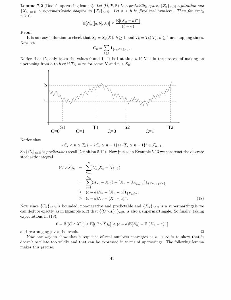
Lemma 7.2 (Doob’s upcrossing lemma). Let (Ω,F , P) be a probability space, Fnn∈N a filtration andXnn∈N a supermartingale adapted to Fnn∈N. Let a < b be fixed real numbers. Then for everyn ≥ 0,

E[Nn([a, b],X)] ≤ E[(Xn − a)−]

(b − a).

Proof

It is an easy induction to check that Sk = Sk(X), k ≥ 1, and Tk = Tk(X), k ≥ 1 are stopping times.Now set

Cn =∑

k≥1

1Sk<n≤Tk.

Notice that Cn only takes the values 0 and 1. It is 1 at time n if X is in the process of making anupcrossing from a to b or if TK = ∞ for some K and n > SK .

T2

b

a

S1C=0 C=1

T1C=0

S2C=1

Notice thatSk < n ≤ Tk = Sk ≤ n − 1 ∩ Tk ≤ n − 1c ∈ Fn−1.

So Cnn∈N is predictable (recall Definition 5.12). Now just as in Example 5.13 we construct the discretestochastic integral

(C X)n =

n∑

k=1

Ck(Xk − Xk−1)

=

Nn∑

i=1

(XTi− XSi

) + (Xn − XSNn+1)1SNn+1≤n

≥ (b − a)Nn + (Xn − a)1Xn≤a

≥ (b − a)Nn − (Xn − a)−. (18)

Now since Cnn∈N is bounded, non-negative and predictable and Xnn∈N is a supermartingale wecan deduce exactly as in Example 5.13 that (C X)nn∈N is also a supermartingale. So finally, takingexpectations in (18),

0 = E[(C X)0] ≥ E[(C X)n] ≥ (b − a)E[Nn] − E[(Xn − a)−]

and rearranging gives the result. 2

Now one way to show that a sequence of real numbers converges as n → ∞ is to show that itdoesn’t oscillate too wildly and that can be expressed in terms of upcrossings. The following lemmamakes this precise.

41

Lemma 7.3. A real sequence xnn∈N converges to a limit in [−∞,∞] if and only if N([a, b], x) < ∞for all a, b ∈ R with a < b.

Proof

Because we need to be able to take a, b rational in our next theorem, we’ll show that xnn∈N doesnot converge if and only if there exist rationals a < b such that N([a, b], x) = ∞.

(i) If N([a, b], x) = ∞, thenlim infn→∞

xn ≤ a < b ≤ lim supn→∞

xn

and so xnn∈N does not converge.(ii) If xnn∈N does not converge, then

lim infn→∞

xn < lim supn→∞

xn

and so choose two rationals a < b in between. 2

Now a supermartingale Xnn∈N is just a random sequence and by Doob’s Upcrossing Lemma wecan bound the number of upcrossings of [a, b] that it makes for any a < b and so our hope is that wecan combine this with Lemma 7.3 to show that the random sequence Xnn∈N converges. This is ournext result.

Theorem 7.4 (Doob’s Forward Convergence Theorem). Let (Ω,F , P) be a probability space andFnn∈N a filtration. Suppose that Xnn∈N is a supermartingale adapted to Fnn∈N with the propertythat

supn

E[|Xn|] < ∞

(we say that Xnn∈N is bounded in L1), then Xnn∈N converges with probability one to an a.s. finitelimit X∞.

Proof

Fix rationals a < b. Then by Doob’s Upcrossing Lemma

E[Nn([a, b],X)] ≤ E[(Xn − a)−]

(b − a)≤ E[|Xn| + a]

(b − a)

and so by the MCT,

E[N([a, b],X)] ≤ supn E[|Xn| + a]

(b − a)

which implies that N([a, b],X) < ∞ a.s.. That is P[N([a, b],X) < ∞] = 1 for any a < b ∈ Q. Hence

P

[ ⋂

a<b∈Q

N([a, b],X) < ∞]

= 1

(since a countable union of null sets is null). So Xnn∈N converges a.s. to some X∞. It remains tocheck that X∞ is finite a.s. But Fatou’s Lemma gives

E[|X∞|] ≤ lim infn→∞

E[|Xn|]

and the right hand side is finite by assumption. Hence |X∞| < ∞ a.s.. 2

Corollary 7.5. If Xnn∈N is a non-negative supermartingale, then X∞ = limn→∞ Xn exists a.s.

42

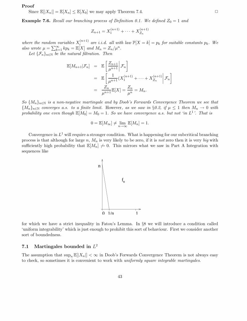
Proof

Since E[|Xn|] = E[Xn] ≤ E[X0] we may apply Theorem 7.4. 2

Example 7.6. Recall our branching process of Definition 0.1. We defined Z0 = 1 and

Zn+1 = X(n+1)1 + · · · + X

(n+1)Zn

where the random variables X(n+1)i are i.i.d. all with law P[X = k] = pk for suitable constants pk. We

also wrote µ =∑∞

k=1 kpk = E[X] and Mn = Zn/µn.Let Fnn∈N be the natural filtration. Then

E[Mn+1|Fn] = E

[Zn+1

µn+1

∣∣∣∣Fn

]

= E

[1

µn+1(X

(n+1)1 + · · · + X

(n+1)Zn

∣∣∣∣Fn

]

=Zn

µn+1E[X] =

Zn

µn= Mn.

So Mnn∈N is a non-negative martingale and by Doob’s Forwards Convergence Theorem we see thatMnn∈N converges a.s. to a finite limit. However, as we saw in §0.2, if µ ≤ 1 then Mn → 0 withprobability one even though E[M0] = M0 = 1. So we have convergence a.s. but not ‘in L1’. That is

0 = E[M∞] 6= limn→∞

E[Mn] = 1.

Convergence in L1 will require a stronger condition. What is happening for our subcritical branchingprocess is that although for large n, Mn is very likely to be zero, if it is not zero then it is very big withsufficiently high probability that E[Mn] 6→ 0. This mirrors what we saw in Part A Integration withsequences like

f

10

n

n

1/n

for which we have a strict inequality in Fatou’s Lemma. In §8 we will introduce a condition called‘uniform integrability’ which is just enough to prohibit this sort of behaviour. First we consider anothersort of boundedness.

7.1 Martingales bounded in L2

The assumption that supn E[|Xn|] < ∞ in Doob’s Forwards Convergence Theorem is not always easyto check, so sometimes it is convenient to work with uniformly square integrable martingales.

43

Definition 7.7 (Martingales bounded in Lp). Let (Ω,F , P) be a probability space, Fnn∈N a filtrationand Mnn∈N a martingale adapted to Fnn∈N. We say that Mnn∈N is bounded in Lp (or for p = 2‘uniformly square integrable’) if

supn

E[|Mn|p] < ∞.

Suppose that Mnn∈N is a uniformly square integrable martingale and that k > j ≥ 0. We adoptthe convention that M−1 = 0. Then

E[(Mk − Mk−1)(Mj − Mj−1)] = E [E [(Mk − Mk−1)(Mj − Mj−1)|Fk−1]] (tower property)

= E [(Mj − Mj−1)E[Mk − Mk−1)|Fk−1]] (taking out what is known)

= 0. (martingale property)

This allows us to obtain a ‘Pythagoras rule’:

E[M2n] = E

(

n∑

k=1

(Mk − Mk−1)

)2

= E[M20 ] +

n∑

k=1

E[(Mk − Mk−1)2] + 2

∑

n≥k>j≥1

E[(Mk − Mk−1)(Mj − Mj−1)]

= E[M20 ] +

n∑

k=1

E[(Mk − Mk−1)2]. (19)

Theorem 7.8. Let (Ω,F , P) be a probability space, Fnn∈N a filtration and Mnn∈N a martingaleadapted to Fnn∈N. The martingale Mnn∈N is uniformly square integrable if and only if

∑

k≥1

E[(Mk − Mk−1)2] < ∞ (20)

and in this case Mn → M∞ a.s. and

limn→∞

E[(Mn − M∞)2] = 0,

that is Mn → M∞ in L2.

Proof

From (19) it is clear that (20) is equivalent to uniform square integrability.Now suppose (20) holds. From Jensen’s inequality (since c(x) = x2 is convex)

E[|Mn|]2 ≤ E[M2n]

and so Doob’s Forward Convergence Theorem shows that M∞ = limn→∞ Mn exists a.s. To checkconvergence in L2 we use Pythagoras again,

E[(Mn+k − Mn)2] =

n+k∑

j=n+1

E[(Mj − Mj−1)2], (21)

and so by Fatou’s Lemma

E[(M∞ − Mn)2] = E[lim infk→∞

(Mn+k − Mn)2]

≤ lim infk→∞

E[(Mn+k − Mn)2]

=∑

j≥n+1

E[(Mj − Mj−1)2] (using (21))

44

and since∞∑

j=1

E[(Mj − Mj−1)2] < ∞

(which is (20)) the right hand side tends to zero as n → ∞. That is

limn→∞

E[(M∞ − Mn)2] = 0

as required. 2

Notice that martingales that are bounded in L2 form a strict subset of those that are boundedin L1 (that is those for which we proved Doob’s Forwards Convergence Theorem). And convergencein L2 implies convergence in L1, so for these martingales we don’t have the difficulty we had withour branching process example. L2-boundedness is often relatively straightforward to check, so isconvenient, but it is a stonger condition than we need for L1-convergence.

8 Uniform Integrability

If X is an integrable random variable (that is E[|X|] < ∞) and Λn is a sequence of sets with P[Λn] → 0,then E[|X1Λn |] → 0 as n → ∞. (This is a consequence of the DCT since |X| dominates |X1Λn | and|X1Λn | → 0 a.s.) Uniform integrability demands that this type of property holds uniformly for randomvariables from some class.

Definition 8.1 (Uniform Integrability). A class C of random variables is called uniformly integrableif given ǫ > 0 there exists K ∈ (0,∞) such that

E[|X|1|X|>K] < ǫ for all X ∈ C.

There are two reasons why this definition is important:

1. Uniform integrability is necessary and sufficient for passing to the limit under an expectation,

2. it is often easy to verify in the context of martingale theory.

Property 1 should be sufficient to guarantee that uniform integrability is interesting, but in fact uniformintegrability is not often used in analysis where it is usually simpler to use the MCT or the DCT. It isonly taken seriously in probability and that is because of 2.

Proposition 8.2. Suppose that Xα, α ∈ I is a uniformly integrable family of random variables onsome probability space (Ω,F , P). Then

1.sup

αE[|Xα|] < ∞,

2.P[|Xα| > N ] → 0 as N → ∞, uniformly in α.

3.E[|Xα|1Λ] → 0 as P[Λ] → 0, uniformly in α.

Conversely, either 1 and 3 or 2 and 3 implies uniform integrability.

45

Proof

1 By definition of uniform integrability, there exists N0 such that for all α

E[|Xα|1|Xα|>N0] ≤ 1.

Then for all α

E[|Xα|] = E[|Xα|1|Xα|≤N0 + |Xα|1|Xα|>N0

]≤ N0P[|Xα| ≤ N0] + 1 ≤ N0 + 1.

Now 1 implies 2 since

P[|Xα| > N ] ≤ 1

NE[|Xα|] (Chebyshev)

≤ 1

Nsup

αE[|Xα|]

and the bound on the right, which evidently tends to zero as N → ∞, is independent of α.To see 3, fix ǫ > 0 and choose Nǫ such that

E[|Xα|1|Xα|>Nǫ] <ǫ

2for all α.

Then choose δ = ǫ/(2Nǫ) and suppose P[Λ] < δ, then

E[|Xα|1Λ] = E[|Xα|1Λ∩|Xα|≤Nǫ + |Xα|1Λ∩|Xα|>Nǫ]

≤ NǫE[1Λ] + E[|Xα|1Λ∩|Xα|>Nǫ]

≤ NǫP[Λ] +ǫ

2< ǫ independent of α.

Thus, given ǫ > 0, choosing δ in this way, P[Λ] < δ implies E[|Xα|1Λ] < ǫ as required.For the converse, since 1 implies 2, it is enough to check that 2 and 3 imply uniform integrability.

Choose ǫ > 0, by 3 there exists δ > 0 such that P[Λ] < δ implies E[|Xα|1Λ] < ǫ for all α. Then sinceby 2 there is N0 such that N ≥ N0 implies P[|Xα| > N ] < δ for all α, we have that for all N ≥ N0

E[|Xα|1|Xα|>N

]< ǫ for all α.

2

We’ve already said that uniform integrability is a necessary and sufficient condition for going tothe limit under the integral. Let’s state this a bit more formally. Recall that for a family of randomvariables Xnn∈N on (Ω,F , P) we say that Xn → X in L1 if

E[|Xn − X|] → 0 as n → ∞.

We say that Xn → X in probability if given ǫ > 0

limn→∞

P [ω : |Xn(ω) − X(ω)| > ǫ] = 0.

It’s easy to check that if Xn → X in L1, then for any set Λ

E [|Xn1Λ − X1Λ|] → 0 as n → ∞.

Theorem 8.3 (Uniform Integrability and L1 convergence). Let Xnn∈N be a sequence of integrablerandom variables which converge in probability to a random variable X. TFAE

46

1. Xnn∈N is uniformly integrable,

2. E[|Xn − X|] → 0 as n → ∞,

3. E[|Xn|] → E[|X|] as n → ∞.

Proof

Since |Xn| → |X| in probability, by Theorem 3.14 there exists a subsequence nkk∈N such thatXnk

k∈N converges a.s.. Fatou’s Lemma gives

E[|X|] ≤ lim infn→∞

E[|Xnk|]

and by Proposition 8.2 1 the right hand side is bounded. Thus X is integrable. Now let ǫ > 0.

E[|X − Xn|] = E[|X − Xn|1|X−Xn|≤ǫ/3 + |X − Xn|1|X−Xn|>ǫ/3]

≤ ǫ

3+ E

[|X|1|X−Xn|>ǫ/3 + |Xn|1|X−Xn|>ǫ/3

].

Now since Xn → X in probability we have P[|X − Xn| > ǫ/3] → 0 as n → ∞ and so using theintegrability of X and the DCT gives

E[|X|1|X−Xn|>ǫ/3] → 0 as n → ∞.

Since by Proposition 8.2 3, uniform integrability implies

E[|Xn|1|X−Xn|>ǫ/3] → 0 as n → ∞,

we haveE[|Xn − X|] → 0 as n → ∞

as required.2 implies 3 is obvious, so let’s prove that 3 implies 1.Suppose then thet E[|Xn|] → E[|X|] as n → ∞. For any real number M such that P[X = M ] = 0,

we define

X(M) =

X |X| ≤ M,0 |X| > M,

with a parallel definition for X(M)n .

Then for any such M ,

E[|Xn|1|Xn|>M] = E[|Xn|] − E[|X(M)n |]

→ E[|X|] − E[|X(M)|]

as n → ∞ since E[|Xn|] → E[|X|] by hypothesis and using the bounded convergence theorem.Now let ǫ > 0. Choose Mǫ large enough that

E[|X|] − E[|X(Mǫ)|] <ǫ

3

(and P[|X| = Mǫ] = 0 as above). There exists N0 such that for n ≥ N0 we have both

|E[|Xn|] − E[|X|]| <ǫ

3

47

and ∣∣∣E[|X(Mǫ)n |] − E[|X(Mǫ)|]

∣∣∣ <ǫ

3.

Then for all n ≥ N0,

E[|Xn|1|Xn|>Mǫ] = E[|Xn|] − E[|X(Mǫ)n |]

≤∣∣∣E[|X|] − E[|X(Mǫ)|]

∣∣∣+ |E[|Xn|] − E[|X|]| +∣∣∣E[|X(Mǫ)

n |] − E[|X(Mǫ)|]∣∣∣

<ǫ

3+

ǫ

3+

ǫ

3= ǫ

There are only finitely many n < N0, so there exists M ′ǫ ≥ Mǫ such that

E[|Xn|1|Xn|>M ′

ǫ

]< ǫ

for all n, which is 1. 2

The second reason that uniform integrability is important is that it is readily verified for martingalesand submartingales.

Theorem 8.4. Let Fαα∈I be a family of sub σ-fields of F and let X be an integrable random variable.Define

Xα = E[X|Fα].

Then Xα, α ∈ I is uniformly integrable.

Proof

Let Y = E[X|Fα]. By the conditional Jensen inequality (Proposition 4.12), since c(x) = |x| isconvex,

|Y | = |E[X|Fα]| ≤ E [ |X|| Fα] a.s.

and soE[|Y |1|Y |≥K] ≤ E

[E[ |X|| Fα]1|Y |≥K

]= E[|X|1|Y |≥K]. (22)

Now the single integrable random variable X forms on its own a uniformly integrable class and soby Proposition 8.2 given ǫ > 0 we can find δ > 0 such that P[Λ] < δ implies E[|X|1Λ] < ǫ. So toshow that (22) is less than ǫ for sufficiently large K we must check that P[|Y | ≥ K] converges to zero(uniformly in α) as K → ∞. But

P[|Y | ≥ K] ≤ E[|Y |]K

(Chebyshev)

=E[|X|]

K(tower property)

so for any α, taking K > E[|X|]/δ implies P[|Y | ≥ K] < δ and hence the right hand side of (22) is lessthan ǫ as required. 2

Theorem 8.5. Let (Ω,F , P) be a probability space, Fnn∈N a filtration and Mnn∈N a martingaleadapted to Fnn∈N. TFAE

1. Mnn∈N is uniformly integrable,

2. Mn converges a.s. and in L1(Ω,F , P) to a limit M∞,

3. there exists Z ∈ L1(Ω,F , P) such that Mn = E[Z|Fn], n ≥ 0

48

Proof

We already have most of the ingredients.1 =⇒ 2: If Mnn∈N is uniformly integrable then it is bounded in L1 and so by Doob’s Forward

Convergence Theorem it converges a.s.. Theorem 8.3 and uniform integrability ensure convergence inL1 to a limit which we denote M∞.

2 =⇒ 3: Choose Z = M∞. For all m,n ∈ N with m ≥ n and all F ∈ Fn

E[Xm1F ] = E[Xn1F ]

(combining Xn = E[Xm|Fn] a.s. and the tower property) and letting m → ∞ , the L1 convergencegives

E[X∞1F ] = E[Xn1F ] for all F ∈ Fn

which gives Xn = E[X∞|Fn] a.s. by definition of conditional expectation.3 =⇒ 1 follows directly from Theorem 8.4. 2

9 Backwards Martingales and the Strong Law of Large Numbers

Backwards martingales are martingales for which time is indexed by the negative integers Z.Given sub σ-algebras

G−∞ =⋂

k∈N

G−k ⊆ · · · ⊆ G−(n+1) ⊆ G−n ⊆ · · · ⊆ G0

an integrable G−nn∈N-adapted process M−nn∈N is a backwards martingale if

E[M−n+1|G−n] = M−n a.s.

Backwards martingales are automatically uniformly integrable by Theorem 8.4 since M0 is integrableand

M−n = E[M0|G−n].

We can easily adapt Doob’s Upcrossing Lemma to prove that if Nm([a, b],M) is the number of up-crossings of [a, b] by a backwards martingale between times −m and 0, then

(b − a)E[Nm([a, b],M)] ≤ E[(M0 − a)−]. (23)

To see this consider the forwards martingale M−m+k for 0 ≤ k ≤ m. As m → ∞, Nm([a, b],M)converges a.s. to the total number of upcrossings of [a, b] by M−nn∈N and since the bound in (23) isuniform in m, we conclude, exactly as in Doob’s Forward Convergence Theorem, that M−n convergesa.s. to a G−∞-measurable random variable M−∞ as −n → −∞. As remarked above, our backwardsmartingale is automatically uniformly integrable and so we have:

Theorem 9.1. Let M−nn∈N be a backwards martingale. Then M−n converges a.s. and in L1 as−n → −∞ to the random variable M−∞ = E[M0|G−∞].

We now use this result to prove the celebrated Kolmogorov Strong Law.

Theorem 9.2 (Kolmogorov’s SLLN). Let Xnn∈N be a sequence of i.i.d. random variables withE[|Xk|] < ∞ for each k. Write µ = E[Xk] and define

Sn =

n∑

k=1

Xk.

49

ThenSn

n→ µ a.s. and in L1 as n → ∞.

Proof

DefineG−n = σ(Sn, Sn+1, Sn+2, . . .)

andG−∞ = ∩k∈NG−k.

Note that G−n = σ(Sn,Xn+1,Xn+2, . . .) and that by independence of the Xi’s, G−(n+1) is independentof the sub σ-algebra σ(X1, Sn) (which is a sub σ-algebra of σ(X1,X2, . . . ,Xn)). Thus

E[X1|G−n] = E[X1|σ(Sn, σ(Xn+1,Xn+2, . . .))] = E[X1|Sn].

But by symmetry (recall that Xnn∈N is an i.i.d. sequence)

E[X1|Sn] = E[X2|Sn] = · · · = E[Xn|Sn]

and1

nE[X1 + · · · + Xn|Sn] =

1

nSn.

Therefore, for all n ∈ N

E[X1|G−n] = · · · = E[Xn|G−n] =Sn

n

so that

E[Sn|G−(n+1)] = E[Sn+1|G−(n+1)] − E[Xn+1|G−(n+1)]

= Sn+1 −Sn+1

n + 1=

n

n + 1Sn+1.

Hence, setting M−n = Sn/n, M−nn∈N is a backwards martingale with respect to its natural filtration.Thus Sn/n converges a.s. and in L1 to a limit which is a.s. constant by Kolmogorov’s 0-1 law and soit must equal its mean value,

E[ lim−n→−∞

E[X1|G−n]] = lim−n→−∞

E[E[X1|G−n]]

= limn→∞

E[Sn

n] = µ.

2

Note that the result is not completely obvious. For example, if the Xi are normally distributedwith mean zero and variance 1, Sn/n converges to zero a.s., but Sn/

√n does not converge and indeed

lim sup Sn/√

2n log log n = 1.

50

Index

L1-bounded, 42L2-martingale, 35, 43π-system, 5σ-algebra, 4

Borel, 5generated by a collection of sets, 5generated by a random variable, 14independence of collection, 13product, 11tail, 18

absolutely continuous, 26adapted process, 30algebra, 4almost everywhere, 9almost sure convergence, 20almost surely, 9angle bracket process, 35

backwards martingale, 49Bayes’ rule, 23BC1, 16BC2, 17Borel σ-algebra, 5Borel measure, 5Borel-Cantelli Lemma, 16branching process, 2, 43

Chebyshev’s inequality, 22compensation, 34conditional convergence theorems, 28conditional expectation, 2, 23

a.s. uniqueness, 25and mean square approximation, 30defining relation, 24existence, 26taking out what is known, 28tower property, 28

conditional Jensen’s inequality, 29consistent family, 15convergence

almost surely, 20, 21in Lr, 20in distribution, 20in probability, 20, 21

convex function, 22

cylinder sets, 15

defining relation (conditional expectation), 24discrete measure theory, 5discrete stochastic integral, 33distribution function, 8, 10Dominated Convergence Theorem, 10Doob’s forward convergence theorem, 42

extinction probability, 2

Fatou’s Lemma, 10reverse, 10

filtration, 30natural, 31

Fubini’s Theorem, 12

Galton-Watson branching process, 2, 43

image measure, 11independent

σ-algebras, 13events, 13random variables, 14

integrable function, 9

Jensen’s inequality, 22conditional version, 29

Kolmogorov 0-1 Law, 19Kolmogorov’s Consistency Theorem, 15

law of the iterated logarithm, 19Lebesgue-Stieltjes measure, 8liminf, 9

sets, 15limsup, 9

sets, 15

martingale, 4, 31backwards, 49

martingale convergence theorem, 42martingale difference, 33martingale transform, 33maximal inequality, 39measurable function, 9measure space, 4

51

monotone convergence properties, 6modes of convergence, 20monotone class, 13Monotone Class Theorem, 13monotone convergence properties, 6Monotone Convergence Theorem, 10

natural filtration, 31

Optional Stopping Theorem, 36optional time, 36

partition, 24Partition Theorem, 24, 29predictable process, 33product σ-algebra, 11product measure, 12

Radon measure, 5Radon-Nikodym derivative, 26Radon-Nikodym Theorem, 26random variable, 10

equivalence class, 23independent, 14

reverse Fatou Lemma, 10

Scheffe’s Lemma, 10set function, 6simple function, 9

canonical form, 9standard machine, 12stopped martingale, 34stopping time, 36Strong law of large numbers, 49submartingale, 31supermartingale, 31

tail σ-algebra, 18taking out what is known, 28tower property, 2, 28

uniform integrability, 45and L1 convergence, 46

uniqueness of extension, 5upcrossing, 40upcrossing lemma, 41

52