Automatic Task Design on Amazon Mechanical...

Automatic Task Design on Amazon Mechanical Turk

A thesis presented

by

Eric Hsin-Chun Huang

To

Applied Mathematics

in partial fulfillment of the honors requirements

for the degree of

Bachelor of Arts

Harvard College

Cambridge, Massachusetts

April 6, 2010

Abstract

Workers’ behaviors are heavily influenced by factors such as provided reward and the amount

and structure of the work. In this thesis, I study the problem of task design, which is

important because efficient designs can induce workers to adopt behaviors that are desirable

to employers. I present a framework for adopting a quantitative approach to design image

labeling tasks on Amazon Mechanical Turk, an online marketplace for labor. With the

idea of learning from observations and the use of machine learning techniques, I first train

workers’ behavior models and use these models to find solutions to the design problems for

different goals. The experimental results show support for the importance of design in this

domain and the validity of the trained models for predicting the quality and quantity of

submitted work.

1

Acknowledgments

I thank my thesis supervisor, Prof. David Parkes, for directing my research along the right

path, for pointing me to the right place when troubled, and for providing encouragement

throughout this project. I thank Haoqi Zhang for the extremely helpful weekly meetings,

and for closely working with me to get past one challenge after another. His passion for

research and thirst for knowledge motivate me to do great work. I thank Prof. Yiling

Chen and Prof. Krzysztof Gajos for their insights on the project and advices from different

perspectives.

Lastly, I thank my parents and my brother, Hank, for providing unending love and

support, and for believing in me.

1

Contents

Abstract 1

Acknowledgments 1

1 Introduction 4

1.1 Problem Statement and Approach . . . . . . . . . . . . . . . . . . . . . . . 5

1.2 Contributions . . . . . . . . . . . . . . . . . . . . . . . . . . . . . . . . . . . 6

1.3 Related Work . . . . . . . . . . . . . . . . . . . . . . . . . . . . . . . . . . . 7

1.4 Outline . . . . . . . . . . . . . . . . . . . . . . . . . . . . . . . . . . . . . . 9

2 Amazon Mechanical Turk and Image Labeling Tasks 10

2.1 Overview of Amazon Mechanical Turk . . . . . . . . . . . . . . . . . . . . . 10

2.1.1 Web Interface for Workers . . . . . . . . . . . . . . . . . . . . . . . . 12

2.1.2 User Communities . . . . . . . . . . . . . . . . . . . . . . . . . . . . 13

2.2 Choosing Tasks . . . . . . . . . . . . . . . . . . . . . . . . . . . . . . . . . . 15

2.2.1 Criteria for Tasks . . . . . . . . . . . . . . . . . . . . . . . . . . . . . 15

2.2.2 Image Labeling Tasks . . . . . . . . . . . . . . . . . . . . . . . . . . 16

2.3 Configuration of a Posting of Image Labeling HITs . . . . . . . . . . . . . . 18

2.4 Design Goals . . . . . . . . . . . . . . . . . . . . . . . . . . . . . . . . . . . 19

1

2

3 Problem Formulation and Design Approach 20

3.1 Problem Formulation . . . . . . . . . . . . . . . . . . . . . . . . . . . . . . . 20

3.1.1 Challenges for Task Design on AMT . . . . . . . . . . . . . . . . . . 22

3.2 Design Approach . . . . . . . . . . . . . . . . . . . . . . . . . . . . . . . . . 23

3.2.1 Idea of Environment Design . . . . . . . . . . . . . . . . . . . . . . . 23

4 Behavior Models 26

4.1 Behavior outside the HIT . . . . . . . . . . . . . . . . . . . . . . . . . . . . 27

4.1.1 View-accept Model Approach . . . . . . . . . . . . . . . . . . . . . . 27

4.1.2 Time Model Approach . . . . . . . . . . . . . . . . . . . . . . . . . . 30

4.2 Behavior within the HIT . . . . . . . . . . . . . . . . . . . . . . . . . . . . . 30

5 Initial Experiment and Model Selection 32

5.1 Setup . . . . . . . . . . . . . . . . . . . . . . . . . . . . . . . . . . . . . . . 32

5.2 Training Models . . . . . . . . . . . . . . . . . . . . . . . . . . . . . . . . . 34

5.2.1 Behavior outside the HIT . . . . . . . . . . . . . . . . . . . . . . . . 34

5.2.2 Behavior within the HIT . . . . . . . . . . . . . . . . . . . . . . . . . 40

5.3 Conclusion . . . . . . . . . . . . . . . . . . . . . . . . . . . . . . . . . . . . 42

6 Designs and Experimental Results 45

6.1 Design Problems . . . . . . . . . . . . . . . . . . . . . . . . . . . . . . . . . 45

6.2 Benchmarks and Our Designs . . . . . . . . . . . . . . . . . . . . . . . . . . 47

6.3 Experiments . . . . . . . . . . . . . . . . . . . . . . . . . . . . . . . . . . . . 51

6.3.1 Setup . . . . . . . . . . . . . . . . . . . . . . . . . . . . . . . . . . . 51

6.3.2 Results and Discussion . . . . . . . . . . . . . . . . . . . . . . . . . . 51

3

7 Conclusion 59

7.1 Brief Review . . . . . . . . . . . . . . . . . . . . . . . . . . . . . . . . . . . 59

7.2 Future Work . . . . . . . . . . . . . . . . . . . . . . . . . . . . . . . . . . . 60

7.3 Conclusion . . . . . . . . . . . . . . . . . . . . . . . . . . . . . . . . . . . . 61

Bibliography 62

Chapter 1

Introduction

Online crowdsourcing is a problem-solving model where tasks traditionally performed by

in-house employees and contractors are brought to online communities to be completed.

It is beginning to find a significant influence in both the business world and academia.

Businesses are using online crowdsourcing to obtain a cheap on-demand workforce, while

academic communities in various fields, such as economics, psychology, and computer sci-

ence, are using online crowdsourcing as a convenient source of subjects for experiments. It

becomes important to understand how employers/requesters can gain knowledge of such an

environment, and how they can use that knowledge to achieve their interested goals.

Amazon Mechanical Turk (AMT) is an online marketplace that facilitates online crowd-

sourcing by bringing requesters and workers together [20]. The name comes from the name

of a chess-playing automaton of the 18th century, which concealed the presence of a human

chess master who was controlling its operations behind the scene. Originally developed for

Amazon’s in-house use, AMT was launched in 2005 [1]. Its application programming in-

terface (API) enables computers to coordinate human intelligence to accomplish tasks that

are difficult for computers, thus the associated term “artificial artificial intelligence.” The

platform allows requesters (humans or computers) to post human intelligence tasks (HITs)

and registered workers to choose to complete such tasks in exchange for specified monetary

rewards.

4

5

1.1 Problem Statement and Approach

In this thesis, I am interested in computer science methods for learning about the worker

population on the AMT domain, and how this knowledge can be used to design tasks for

different goals. Specifically, I consider image labeling tasks where workers are asked to label

a set of images, each with a required certain number of tags describing the contents of the

image or some relevant context. The designs refer to choosing a set of parameters for HITs,

such as reward amount per HIT, number of images per HIT, number of labels required per

image, number of assignments per HIT, total number of HITs, and time to post. I consider

two goals for design: 1) quality, to obtain the most number of labels in the gold standard,

and 2) quantity, to obtain the most number of labels regardless of whether they are in the

gold standard, both under budget and time constraints.

For a particular goal, it is not obvious how the requester would set those parameters

so that the collective behavior of the workers align with the goal. In order to design, the

requester needs to understand how the worker population behaves with respect to the design

and how the behavior changes as the design is modified. The approach taken in this thesis

adopts the idea of environment design as well as standard machine learning techniques.

Environment design studies problems in settings where an interested party aims to influ-

ence an agent’s behavior by providing limited changes to the agent’s environment. Recent

theoretical work by Zhang et al. [25] includes a framework to solve environment design

problems by learning from observations of agent behaviors in order to effectively design.

Environment design is fitting to our problem because we can think of the AMT domain

and HITs as the environment, the worker population as the agent, and the requester as the

designer of the environment. For learning from observations, machine learning techniques

are used to predict future outcomes of designs.

There are several challenges:

• Need to understand how the worker population behaves.

We need to understand how the worker population behaves with respect to different

6

designs, so that we can evaluate different designs to choose the optimal for a particular

goal.

• Need to understand which environment variables are important.

We need to know which of the environment variables significantly affect the popula-

tion’s behavior to make sure the important ones are included in the behavior model,

while the less important ones are excluded to reduce problem complexity.

• The environment is not fully observable.

The Amazon Mechanical Turk API is limited in providing system-wide statistics, such

as total current online workers and completed HITs over a given time period, which

may be insufficient for learning about an agent’s preferences to work on a given HIT

that we post.

• Need to know which machine learning algorithms to use.

We need to find out which machine learning algorithms are suitable to this problem

and domain.

1.2 Contributions

In this thesis, I present a framework for automatic designing image labeling tasks on AMT.

Adopting a quantitative approach to design, I formulate a model-based view on how workers

act on AMT, and train models to predict workers’ behaviors. Using these trained models,

I formulate the design problems as optimization problems, and search for solutions. The

experimental results show support for the importance of design in this domain and for using

our trained model to design. This work serves as the initial attempt to adopt quantitative

behavior models to design.

7

1.3 Related Work

Prior work by Zhang et al. [26, 28, 27, 25] laid out a solid theoretical foundation for the

problem of environment design. Using the inverse reinforcement learning framework and the

idea of active indirect preference elicitation, Zhang and Parkes developed a method to learn

the reward function of the agent in a Markov Decision Process (MDP) setting and proved

the method’s convergence to desirable bounds [26, 28]. Zhang and Parkes also showed that

value-based policy teaching is NP-hard and provided a mixed integer program formulation

[27]. Our application is built on the theoretical work on a general approach to environment

design, where Zhang et al. [25] presented a general framework for the formulation and

solution of environment design problems with one agent.

However, the above-mentioned theoretical work is not be easily applicable to the AMT

domain. First, the theories are based on linear programs and MDPs for modeling an

agent’s behavior in the domain, which may not be suitable for describing agent behavior

on AMT. Second, the iterative learning approach in Zhang’s work cuts down the parameter

space of the behavior model by some inverse learning method, e.g. inverse linear programs

for linear programming models and inverse reinforcement learning for MDP models. This

inverse method might not be available for the specific models chosen for the AMT domain.

Third, the learning process might need to be modified by adding slack variables or making

it probabilistic because the AMT domain is very volatile as the number of HITs on the

system and the activity level as approximated by logging completed HITs both vary quite

a bit from day to day.

Some work has been done on studying the nature of the workforce on AMT. Snow et

al. [16] used AMT for five human linguistic annotation tasks, and found high agreement

between the AMT non-expert annotations and the existing gold standard labels provided

by experts. This is in support of obtaining high quality work using AMT.

Sorokin and Forsyth [17] also use AMT to obtain data annotation, and began some

analysis on the workforce by noting the high elasticity of the workforce and that roughly

top 20% of annotators produce 70% of the data across different tasks. However, the analysis

8

of the workforce is brief and only note qualitative observations. It also did not include how

environment variables affect workers’ behavior.

Su et al. [18] conducted experiments on AMT also with several kinds of tasks. They

varied the qualification test score needed for a worker to do a task and voting schemes

for answers, and observed their effects on work quality. Generally, they saw that higher

qualification score led to higher accuracy and lower number of workers, as expected.

Mason and Watts [11] studied the relationship between financial incentives and perfor-

mance on AMT, and found that increased financial incentives increase quantity, but not

quality of work. They attempted to explain this with the “anchoring” effect that workers’

perceived value of their work depend on the amount they are paid.

None of the work mentioned above provided quantitative models for describing the be-

havior of the worker population on AMT. In this thesis, I aim to develop a mathematical

model for prediction that can be used in task designs.

There has also been work on different methods of collecting image labels. Image labeling

is only one kind of task that concerns enterprise and content management systems, referred

to as ACE (attribute extraction, categorization and entity resolution) by Su et al.[18].

Common ways to accomplish these tasks are to have in-house workers, and to outsource

them to contract workers. However, these approaches face scalability limitations, and this

is where systems such as Google Image Labeler [10] and AMT come in. In [24], Yuen et

al. gave an extensive survey of human computation systems. Of particular relevance are

LabelMe [13] and the ESP game [23]. LabelMe is a web-based tool for image annotation,

which asks users to draw and label polygons corresponding to items in the images. The tool

allows anyone to label any number of images he/she wants. Users can also adopt this tool

to label their own sets of images, provided that they are uploaded to the LabelMe database.

The ESP game, pioneered by Luis Von Ahn et al., is one kind of GWAP (game with a

purpose) that were made for a variety of different human computation tasks. The ESP game

works by showing a sequence of images to a random pair of two random players and asking

them to provide labels describing the image. When a match between labels submitted by

9

the two players is found, they advance to the next image. If the image shown is already

labeled, the labels may appear as taboo words, so entering them repeatedly will not advance

the players to the next image. The goal for the players is to get as many matches as possible

within the time limit.

Each of these different approaches has its pros and cons, as described by Deng et al.

[4]. The LabelMe dataset was critiqued on its small number of categories, but it provides

outlines and locations of objects. For the ESP game, one advantage is that by incentivizing

people to contribute by making the task fun, it acquires labels for free and very quickly.

However, one drawback mentioned is that its speeded nature may promote certain strategies

to provide “basic level” words as labels, as opposed to more specific or general level.

AMT has been used by some [4, 17, 13] for constructing image datasets. With the

flexibility to use different approaches such as using the LabelMe web-tool and the ImageNet

method, AMT can be used to build datasets of different advantages and drawbacks for

different needs.

1.4 Outline

In Chapter 2, I give an overview of the AMT domain and image labeling tasks. In Chapter

3, I formulate the design problem of image labeling tasks on AMT, discuss the challenges

and present a design approach. In Chapter 4, I propose mathematical models for describing

workers’ behavior. In Chapter 5, I present results from the initial experiment, train and

evaluate the proposed models, and select the best-performing models. In Chapter 6, I use

the selected models to formulate the design problems, and present experimental results.

Finally, I conclude in Chapter 7.

Chapter 2

Amazon Mechanical Turk and

Image Labeling Tasks

Amazon Mechanical Turk [20] is a marketplace for work that requires human intelligence.

Since its launch in 2005 (still in beta), a wide variety of tasks have been completed on AMT.

Some examples listed on the AMT website include:

• Select the correct spelling for these search terms.

• Is this website suitable for a general audience?

• Transcribe conversations in this audio.

• Write a summary for this article.

In this chapter, I provide an overview of Amazon Mechanical Turk and a detailed de-

scription of the chosen task for design in this thesis – image labeling.

2.1 Overview of Amazon Mechanical Turk

Some key concepts of AMT are described below:

10

11

• Human Intelligence Task (HIT)

A minimal unit of work that a worker can do.

• Requester

A user who posts HITs on the system.

• Turker/worker

A registered user who does work on the system.

• Reward

The amount of money the requester pays for a HIT.

• Assignments

An assignment is created when a worker accepts a HIT, and belongs uniquely to that

particular worker. The requester can specify how many assignments can be created

for a HIT, which is equivalent to the maximum number of workers who can work on

a single HIT.

On AMT, requesters can post any HITs for registered workers to complete. After an

assignment is submitted, the requester reviews the work and chooses to approve or reject

it. If the assignment is rejected, the requester is not obligated to pay the worker. Amazon

charges the maximum of 10% of the reward amount and half a cent for fees. In addition to

the web interface, AMT provides REST1 and SOAP2 application programming interfaces

(APIs), as well as a command-line interface for programmable interactions with the system.

For a group of HITs, the requester specifies the reward per HIT, number of assignments

per HIT, its lifetime during which the HITs will be available to workers, the amount of

time the workers have to complete a single HIT, and optionally a qualification requirement

for workers to be eligible to do the task. AMT has default qualification criteria requesters

1REST, Representational State Transfer, is style of software architecture for distributed hypermediasystems such as the World Wide Web [http://en.wikipedia.org/wiki/Representational State Transfer/].

2SOAP, originally defined as Simple Object Access Protocol, is a protocol specification forexchanging structured information in the implementation of Web Services in computer networks[http://en.wikipedia.org/wiki/SOAP/].

12

can use, including percentages of tasks accepted, completed, approved, rejected, etc, as well

as worker locale. The requester can also create custom qualification tests using the AMT

API. These tests could be an example HIT, or could be a completely different task used to

determine the workers’ eligibility as deemed appropriate by the requester. HITs can also

be extended/terminated at any time by the requester. As a measure to ensure anonymity,

AMT assigns a worker ID to each worker account. The requester can see the worker’s ID if

he/she has completed one of the posted HITs, but the requester cannot retrace the worker’s

identity from his/her ID.

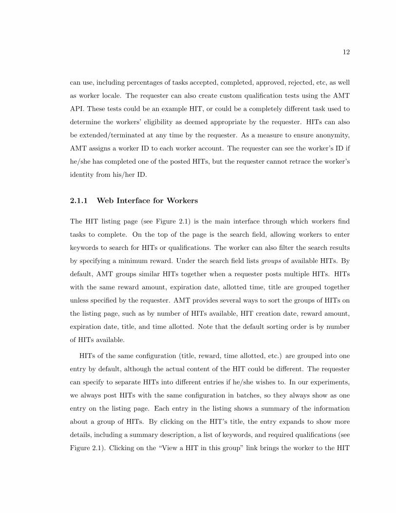
2.1.1 Web Interface for Workers

The HIT listing page (see Figure 2.1) is the main interface through which workers find

tasks to complete. On the top of the page is the search field, allowing workers to enter

keywords to search for HITs or qualifications. The worker can also filter the search results

by specifying a minimum reward. Under the search field lists groups of available HITs. By

default, AMT groups similar HITs together when a requester posts multiple HITs. HITs

with the same reward amount, expiration date, allotted time, title are grouped together

unless specified by the requester. AMT provides several ways to sort the groups of HITs on

the listing page, such as by number of HITs available, HIT creation date, reward amount,

expiration date, title, and time allotted. Note that the default sorting order is by number

of HITs available.

HITs of the same configuration (title, reward, time allotted, etc.) are grouped into one

entry by default, although the actual content of the HIT could be different. The requester

can specify to separate HITs into different entries if he/she wishes to. In our experiments,

we always post HITs with the same configuration in batches, so they always show as one

entry on the listing page. Each entry in the listing shows a summary of the information

about a group of HITs. By clicking on the HIT’s title, the entry expands to show more

details, including a summary description, a list of keywords, and required qualifications (see

Figure 2.1). Clicking on the “View a HIT in this group” link brings the worker to the HIT

13

page where the worker can preview one of the actual HITs and decide whether to accept

it. Figure 2.2 shows an example of an actual HIT. Once the HIT is accepted, the worker

gets to work on the HIT and a submit button appears, with a checkbox that automatically

accepts the next HIT for the worker when checked.

Figure 2.1: HIT listing page

2.1.2 User Communities

AMT already has a substantial user base that is quite active, and has formed user commu-

nities. For example, Turker Nation [12] is an online forum where people discuss anything

related to AMT, from efficient working strategies to requester reviews. Developer commu-

nities also formed. Scripts were written to increase workers’ productivity, mostly using the

Greasemonkey add-on for Firefox. Some are specifically written for HITs that are popu-

lar and well-supplied. One particularly popular script is Turkopticon [22], which provides

14

Figure 2.2: Actual HIT page

worker-generated requester reviews overlaying the HIT listing page.

On the requester’s side, several tools have also been built to facilitate posting tasks and

running experiments on AMT. Seaweed [2] is a web application for developing economic

games to deploy on the web and AMT. Turkit [21] is a Java/Javascript API for posting

iterative tasks on AMT.

15

2.2 Choosing Tasks

2.2.1 Criteria for Tasks

The AMT platform allows a wide variety of the types of task to be posted. In this thesis, I

choose a specific type of task to design, considering the following criteria:

• High Volume

A large volume of the chosen type of task should be available. This ensures that there

is enough work to be used for learning the model and that there is a good number of

work left so that the learning is worth the effort.

• Self-contained

The chosen type of task should be self-contained, meaning that the variables that

affect the agent’s behavior should be within the task, and that there are limited

external factors influencing the outcome of the work. Workers should not need to

look for outside information in order to complete the task. This secludeness helps the

requester (designer) to have a good understanding and control over the AMT domain

(environment).

• Human-centric

The chosen type of task should be human-centric, fitting the kinds of task that makes

sense for human computation. They should be difficult for computers, but relatively

easy for humans; otherwise, we would not employ AMT.

• Verifiable results

The chosen type of task should have an existing dataset of good-quality work done

for the task. There should be a way to automatically evaluate the submitted results

against the dataset. This dataset can serve as a gold standard which I use to automat-

ically evaluate the quality of the submitted work for the purpose of the experiments.

• Meaningful

16

I aim to choose a type of task that is useful and meaningful for the advancement of

scientific research, particularly the advancement of artificial intelligence research.

2.2.2 Image Labeling Tasks

Image labeling tasks are chosen for design in this work. I will first provide a complete

description of the image labeling tasks, followed by a discussion about how it fits the criteria.

Description of Our Image Labeling HITs

Each HIT pays the worker a specified amount to provide a certain number of labels for

a certain number of images within a specified amount of time. The posted HITs have an

expiration time when uncompleted HITs are no longer available to workers. The guidelines

provided in the HIT are reproduced below:

• For each image, you must provide Ntag distinct and relevant tags.

• You should strive to provide relevant and non-obvious tags.

• Tags must describe the image, contents of the image, or some relevant context.

• Your submitted tags will be checked for appropriateness.

Figure 2.3 is an actual posting of an image labeling task. For this particular image,

labels may include racecars, red, eight, tires, etc.

How It Fits the Criteria

• High Volume

There is an enormous number of images on the web. In 2005, Google has indexed

over one billion images [9]. More and more people are starting to share photos as so-

cial networking websites became increasingly popular. Websites such as ImageShack,

17

Figure 2.3: Actual Image Labeling Task.

Facebook, Photobucket and Yahoo’s Flickr host a total of over 40 billion photos in

2009 [14].

• Self-contained

Each image labeling task is self-contained. The HIT asks for relevant labels that

describe the images, or their content. Workers should not need to look for outside

information to label the images.

• Human-centric

Image labeling is still hard for computers to do. A vast amount of research has been

done on object recognition by the computer vision community. However, most focuses

on images with one or very few objects. To produce non-obvious, or context-implied

labels is even a harder task for computers.

18

• Verifiable results

There are standard image datasets that are commonly used as benchmarks for com-

puter vision algorithms. These include Caltech101/256 [6, 7], MSRC [15], PASCAL [5]

etc. Other datasets include TinyImage [19], ESP dataset [23], LabelMe [13] and Ima-

geNet [4]. One way to verify the results is to run a comparison between the submitted

results and the dataset. If there is overlapping, the submitted labels are considered

valid.

• Meaningful

Labeled images can be used to construct or expand image datasets which can be used

to test computer vision algorithms. When incorporated to search engine databases,

labeled images allow for more accurate and relevant results.

2.3 Configuration of a Posting of Image Labeling HITs

Each component of a posting of image labeling HITs and the notations used is listed:

• R

Amount of reward per HIT paid to the worker.

• Npic

Number of pictures per HIT.

• Ntag

Number of tags required per image.

• NHIT

Total number of HITs posted.

• Nasst

Number of assignments per HIT.

19

• TA

Time allotted per HIT.

• Time

Time of the day when the HITs are posted.

2.4 Design Goals

A requester may be interested in many different goals for image labeling tasks. In this

thesis, I consider two particular goals for design. The first goal, henceforth refered to Goal

1, concerns the quality of the submitted work. It aims to maximize the total number of

submitted labels that are uniquely in the gold standard dataset. The second goal, Goal

2, concerns the quantity of the submitted work. It aims to maximize the total number of

unique labels submitted, regardless of whether they are in the gold standard dataset. For

both goals, a budget constraint and a time limit are imposed so that the experimental results

can be compared. For any particular goal, it is not obvious how the requester would choose

a configuration of the posting so that the workers’ actions are aligned with the requester’s

interests.

Chapter 3

Problem Formulation and Design

Approach

In this chapter, I first formulate the problem of task design for image labeling tasks on AMT,

and discuss the challenges associated with the problem. I give an overview of environment

design and explain why it is fitting for our problem. Finally, I present a sketch of the

adopted design approach.

3.1 Problem Formulation

In this section, I formally specify the design problem for image labeling tasks on AMT. The

requester has many images that he/she wishes to be labeled. The requester posts image

labeling HITs as described in the previous chapter. The requester may choose to post HITs

in several batches in sequence, and can modify the configuration of the posting in between

batches. The requester are allowed to change the following components of a configuration:

• R

Amount of reward per HIT paid to the worker.

• Npic

20

21

Number of images per HIT.

• Ntag

Number of labels asked for per image.

• NHIT

Total number of HITs posted.

• Time

Time of the day when the HITs are posted.

For all HIT postings, Nasst, which denotes the number of assignments per HIT, is fixed

at five, and TA, which denotes the allotted time for completing a single HIT, is fixed at

thirty minutes. Fixing these two variables simplify the design problem while still keeping

its complexity that makes the design problem interesting for the purpose of this work. Five

assignments per HIT is chosen so that the results are not dominated by just one worker.

Thirty minutes is allotted per HIT because it gives the worker plenty of time to complete a

HIT. A configuration of a HIT posting, or a set of values for the above variables, is a design

of the task.

Since the requester is interested in the collective results submitted by the workers for

the two goals, we will view the entire worker population on AMT as a single agent, instead

of viewing each individual worker as an agent. The requester observes the agent’s behavior

by examining the submitted work, in this case, the submitted labels for the images. The

requester also observes other factors such as who (worker’s ID) submits the HITs, when

and how many times each HIT is previewed, accepted and submitted. Furthermore, the

requester observes the page number on which the posted HITs are located in each of the

different sorting orders of the HIT listing page. The requester also collects the system-

wide statistics provided by AMT, such as the number of HITs available and the number of

projects (groups of HITs) available. AMT does not provide the activity level of the workers

at a certain time; however, it may be approximated by counting the number of completed

HITs over a time period by logging every HIT on the system.

22

The design problem is essentially the following question: how can the requester choose

a configuration of a HIT posting that is conducive towards his/her goal?

3.1.1 Challenges for Task Design on AMT

To design tasks on AMT, there are several obstacles:

• Direct queries are infeasible.

Direct queries are infeasible on AMT. Requesters cannot ask workers questions such

as how workers’ actions differ when facing differently structured HITs because it may

be hard to specify their behavior verbally or before actually completing one of the

HITs. For questions like how long it would take to complete fifty of this kind of HIT,

it may be difficult because one worker cannot answer for the population’s collective

behavior. It is possible to ask questions like how much a worker would require to

do a certain kind of HIT by posting the question as a HIT on AMT. However, it is

uncertain whether the workers would answer honestly to questions of this kind, as

strategic workers may report higher or lower numbers.

• Goal-oriented design.

Task design in general is difficult because goals could be complicated. Most requesters

on AMT have some objective when they post tasks. These objectives may concern

the quality and quantity of the result, or the time it takes to complete a batch of

work. Some tasks are easy and mechanical, so the requester may only care about

getting the most number of tasks completed within a time frame. Some tasks might

be more difficult and require creative thinking, so the requester may be interested

in getting the highest quality of work given a budget. Some requesters might have

minimum thresholds for quality and quantity that they want to be able to reach with

the minimal amount of time spent.

• Constraints.

Requesters on AMT face many constraints. First, they have no control over how AMT

23

works, e.g. how the HIT listing page shows available HITs, how workers can search

for HITs, or how much commission Amazon charges for a HIT. These are part of the

domain controlled by Amazon. However, the requesters do have complete control over

the content of the HITs they post (limited by browser capabilities). They are free to

specify the components of a HIT posting however they want. The requesters may also

be under budget constraints, or time constraints associated with their goals.

• Large space of design space.

As mentioned in the previous chapter, a configuration of a HIT posting has many

components such as reward amount, number of images per HIT, number of labels

per image, etc. Treating each of these components as a decision variable, we have a

high-dimensional space of possible designs, each with a large range of values.

• Need a quantitative model describing the workers’ behavior.

In order to design, we need to have an understanding of workers’ behavior and how

it changes with respect to changes in the domain. We need a quantitative model

incorporating environment variables to the workers’ decision problem.

• Large space of agents’ preferences.

For any particular behavior model, we can image workers having quite different pref-

erences for a specific configuration of a HIT posting. Even when we have an under-

standing of the workers’ behavior model, the space of possible preferences may be

large, and we need a method for learning such preferences.

3.2 Design Approach

3.2.1 Idea of Environment Design

The nature of our problem is very similar to the general problem of environment design,

which Zhang et al. [25] formulated as follows. Under the influences of aspects of an en-

vironment, agents act frequently and repeatedly in the environment with respect to their

24

preferences. An interested party observes the agents’ behaviors, either partially or fully.

The interested party can provide limited changes to the environment and observe how

agents’ behaviors change and further learn about the agents’ preferences based on these

observations. By modifying the environment intelligently through repeated interactions,

the interested party aims to align the agents’ behaviors with the decisions desired by the

interested party.

Using active indirect preference elicitation and inverse reinforce learning, Zhang et al.

[28, 27] introduced methods to solve a particular environment design problem, policy teach-

ing, where an agent follows a sequential decision making process modeled by a Markov

Desicion Process (MDP), and an interested party can provide limited incentives to the

states to affect the agent’s policy. Zhang et al. [25] developed a general framework for the

formulation and solution of environment design problems, and applied the framework in a

linear programming setting.

Although the above techniques may not apply to the AMT domain, Zhang’s formulation

of the environment design problem encounters many of the same challenges we face in task

design on AMT:

• Direct queries are infeasible.

Direct queries for preferences may simplify the design problem a lot, simply because it

is much easier to learn about agents’ behavior model. Direct queries may be infeasible

in domains because agents may be uncooperative or dishonest. Another reason may be

that the answers are difficult to specify. An agent can act in an environment; however,

he/she might not be able to specify how each environmental aspect affects his/her

actions. It may also be difficult to describe an agent’s behavioral policy. Finally,

direct queries may be intrusive. Environment design methods makes sense in these

domains because learning from observations is a way to overcome the unavailability

of direct queries.

• Goal-oriented design.

To apply environment design methods, the designer should have a goal that can be

25

clearly specified. The goal should be able to be evaluated based on observations of

agents’ behaviors, so that the designer can learn from past interactions.

• Constraints.

The designer faces constraints in changes that he can make to the environment. These

admissibility constraints would require the designer to modify the environment in an

intelligent way because the constraints eliminate the option of simply trying every

modification of the environment.

• Large space of environment changes.

The space of possible environment changes should be fairly large. This makes the

learning problem interesting: how would the designer choose to change the environ-

ment so that he/she gains a good amount of new information? When the space of

changes is small, the naive method of trying all changes would work reasonably well.

• Need a quantitative model describing the agent’s behavior.

Environment design requires an understanding of the agent decision problem and how

environment changes translate into changes in parameters in the decision problem.

This understanding is the basis that enables learning in the domain.

• Large space of agents’ preferences.

The agents acting in the domain should have a large space of preferences for the

agents’ decision problem. If the space of preferences is small, the designer can just

design for each set of preferences to see which works well.

In the problem of task design on AMT, the environment is the AMT domain itself and

the HITs. The designer of the environment is the requester. The agent in the environment

is the entire worker population. To design, I adopt the environment design’s general idea

of learning from observations and designing based on the learned knowledge. To learn from

observations, I use standard machine learning techniques such as linear regressions, decision

trees, and multilayer perceptrons to discover patterns in the data.

Chapter 4

Behavior Models

In this chapter, I discuss the mathematical models that I consider for describing agent’s

behavior on AMT. The workers’ behavior on AMT can be separated into two parts: 1)

the actions outside the HIT, e.g. how many viewed or accepted the HIT in a given time

frame, and 2) the actions within the HIT, e.g. what they do once they have accepted

the HIT, and what the submitted results are. For behavior outside the HIT, I consider

two approaches. The first approach predicts independently the number of views in a given

time frame and percentage of accepting given the worker views the HIT. The number

of assignments submitted in the time frame can then be predicted by combining the two

models. The second approach directly predicts the time it takes to reach a certain percentage

of completion of the HIT posting. For behavior within the HIT, I consider two models to

predict metrics for each of the 2 interested goals respectively.

26

27

4.1 Behavior outside the HIT

4.1.1 View-accept Model Approach

View Model

The view model predicts the total number of adjusted previews a given HIT configuration

gets. As described before, a worker can first preview a HIT before he/she accepts the HIT.

Once a worker accepts a HIT, he/she can also check a box instructing AMT to automatically

accept the next HIT in the group once the current HIT is submitted. The adjusted number

of previews I track include the actual previews from workers , as well as the views that

come from the automatic accepting after the first HIT. For example, a worker previews a

HIT and decides to accept the HIT. Once he finishes the HIT, he thinks that the HIT is fun

and chooses to check the box to automatically accept the next one. He ends up completing

a total of 5 HITs in the group. In this case, the adjusted number of previews would be

the one preview plus the four views for the subsequent four HITs that were automatically

accepted. This adjustment is made so that the percentage of accepting would be correct

being 100%, instead of 500% without the adjustment.

The following factors are believed to affect the number of previews a HIT posting gets:

• Activity level of workers on AMT.

Higher the activity level of workers on AMT is expected to correspond to higher

number of previews that a HIT posting gets. However, AMT does not provide system-

wide statistics on workers. To approximate the activity level of workers, I track

the total number of completed HITs on the system, assuming that this number is

directionally correlated with the activity level of the workers. I also track the total

number of HITs on the system, used to normalize the number of completed HITs as

the number of completed HITs may depend on how many HITs are available at the

time.

• The page numbers where the group of HITs appear on the listing page in different

28

sorting orders.

The lower the page number is, the more previews the HIT posting gets. However,

different sorting orders may have different magnitude of influence depending on how

workers browse for HITs.

• HIT title of the group, listed keywords, and summary description as can be seen on

the listing page.

These factors are what workers see on the listing page and may affect their decision

to proceed to viewing an example of the HIT posting. However, these factors are kept

constant across HIT postings in our design problem, so I do not consider them in the

model.

To describe the model, I adopt the following notation:

• Rankings = {HITs available, reward amount, ...}

This is the set of different sorting orders a worker can choose for the HIT listing page.

• Pi where i ∈ Rankings

Pi is the page number where the group of HITs appear when sorted according to i

in the beginning of the posting. Note that this number may change as HITs of this

group are completed, and as other HITs are added to or removed from the system.

• CHITs

Completed number of HITs on the system over the time frame when the HITs are

posted.

• THITs

Average total number of HITs on the system over the time frame when the HITs are

posted.

The model is the function f that takes the above variables as inputs and outputs the

total number of previews a particular HIT posting would get:

29

Nviews = f(Pi1 , ..., Pin , CHITs, THITs) (4.1)

where i1, ..., in ∈ Ranking

Some possible forms of the function are:

f =∑

i∈RankingskiCHITsPi

(4.2)

f =∑

i∈Rankingski

logCHITsPi

(4.3)

f =∑

i∈Rankingski

CHITsPiTHITs

(4.4)

where the ki’s are weights associated with each sorting order. Equation 4.2 assumes the

number of previews being linear in CHITs, Equation 4.3 assumes the number of previews

being linear in logCHITs, while Equation 4.4 assumes the number of previews being linear

in CHITs normalized by THITs.

Accept Model

The accept model predicts the percentage of the previews that actually leads to an accepting

of the HIT. In contrast to the factors that affect the number of previews, the relevant factors

here are those present in the content of the HIT:

• R

Reward amount. As reward amount increases, the accepting percentage is likely to

increase because the HIT becomes more attractive to workers when it pays more for

the same amount of work.

• Npic

Number of images per HIT. As the number of images per HIT increases, the accepting

percentage is likely to decrease because completing the HIT requires more work and

thus less attractive to workers.

30

• Ntag

Number of labels required per image. Similar to Npic, as the number of labels re-

quired per image increases, workers need to do more work per HIT, so the accepting

percentage is likely to decrease.

I postulate that the accepting percentage depends on WR , which is the amount of work the

worker does per dollar he/she gets. I assume that a worker makes the decision of whether

to accept based on this value. If this value is over his/her minimum threshold, the worker

accepts after viewing the HIT. I consider a logistic model:

P (accept|preview) =1

1 + e−WR

(4.5)

The possible forms of W may include NpicNtag, Npic logNtag, log(Npic)Ntag, logNpic logNtag,

and log(NpicNtag), where taking the log represents diminishing effect of added work.

4.1.2 Time Model Approach

The second approach directly predicts the time it takes to reach a certain percentage of

completion for a HIT configuration. For example, given the HIT configuration and the time

of the day when the HITs are posted, the model predicts the number of seconds it takes to

get 50% of the posted work submitted. The model is a function that takes the parameters

of a HIT configuration and the time of the day when the HITs are posted as inputs, and

outputs the time it takes (in seconds) to get m% of the posted work completed:

Time = f(R,Npic, Ntag, NHIT , PostingT ime,m) (4.6)

4.2 Behavior within the HIT

For different designs, there are different metrics the designer is interested in using to measure

the submitted work. For Goal 1, the requester is interested in predicting the number of

labels uniquely in the gold standard per assignment for a given HIT configuration. For

31

Goal 2, the requester is interested in predicting the number of unique labels regardless of

the gold standard per assignment for a given HIT configuration. For both goals, we want

to predict the number of labels contributed by a single assignment in order to separate the

predictions of behavior outside the HIT and within the HIT. To obtain the total number

of labels, we simply multiply the number of labels per assignment by the predicted total

number of completed HITs. The possibly influential factors for predicting submitted results

are similar to those for the accept model as important factors are those that can be seen

within a HIT:

• R

Reward amount. The reward amount might affect how workers work by signaling how

much the work is worth to the requester and the quality and quantity that is expected

by the requester.

• Npic

Number of images per HIT. Having too many images per HIT might tire out the

workers, causing them to submit very obvious tags.

• Ntag

Number of labels required per image. Similar to Npic, a high number of labels might

cause the workers to experience fatigue. There might also be diminishing return if the

requester is only interested in unique labels because the chance of overlapping labels

increases in the number of labels requested.

Chapter 5

Initial Experiment and Model

Selection

In this chapter, I present the results from the initial experiment, and select appropriate

models based on training on the obtained dataset.

5.1 Setup

Configurations

In order to select models for predicting behavior, we need to obtain data for different

configurations of HIT postings, so we can evaluate the models on how well they explain the

data. To get this data, I assume that the proposed models are correct and choose informative

configurations that will help verifying the models’ functional forms and assumptions. I chose

a total of 42 different configurations, selected to cover a range of values of important features

in the models. Specifically, I wanted to verify the following models:

• View Model.

The configurations were chosen to have different reward and number of HITs in a

posting to see the effect of different page numbers on the HIT listing page.

32

33

• Accept Model.

The configurations were chosen to cover different W/R values ranging from 0.000833

to 0.0333, where W is assumed to be NpicNtag, which is the total number of labels

required. We can observe how these values affect the percentage of accepting given

the worker views the HIT, and verify whether the threshold values fit a logistic model

within the worker population.

• Behavior within the HIT.

For models predicting the submitted results, we want to vary the factors within the

HIT, e.g. R,Npic, Ntag, and see how they affect the results. The configurations were

chosen by changing each of the variables alone, as well as two and three variables at

a time, such as scaling up reward and amount of work linearly/non-linearly, etc.

These configurations were ran in a random order over a three-week period. Each con-

figuration was allowed to run until completion, and the next configuration was posted

immediately after the completion of the previous one.

Gold Standard Dataset

In order to evaluate the submitted results, we need a gold standard dataset against which

we can compare the submitted labels. I chose the ESP dataset [3] as the gold standard.

The ESP dataset was published by the inventor of the ESP game, Luis von Ahn. It contains

100,000 images with English labels obtained by the ESP Game [23]. This means that all

labels in the dataset were entered by at least two people, and therefore believed to be

relevant to the images and of decent quality. For the use of this work, I filtered the ESP

dataset to contain only those images with at least 10 labels, which are around 57,000 images.

34

5.2 Training Models

I use the popular machine-learning software, Weka [8], to train the proposed models. The

models were evaluated by the leave-one-out cross-validation method. In leave-one-out cross-

validation, the training data is divided into n folds, where n is the number of total training

instances. The model is repeatedly trained on n-2 instances and tested on the validation

set, which is one of the two remaining instances, for n iterations. I choose the best model

based on validation set performance, and report the performance on the test set, which is

the last remaining fold/instance. The evaluation of the model is based on how accurately it

predicts on the test instance. The main metric I consider is RRSE (Root relative squared

error): √∑i(Pi − Ti)2∑i(T − Ti)2

(5.1)

where Pi is the model’s prediction on instance i, Ti is the actual value of instance i, and T

is the average value of the training instances. I also look at MAE (Mean absolute error):

1

n

n∑i=1

|Pi − TiTi

| (5.2)

where Pi is the model’s prediction on instance i, Ti is the actual value of instance i. RRSE

measures how well the trained model predicts as compared to the simple predictor, which

is just the average of the training set. MAE informs about how much the value of the

predictions are off by. Other statistics such as correlation coefficient (CC) and root mean

squared error (RMSE) are also reported. Note that only the results for a subset of different

methods and features are reported here.

5.2.1 Behavior outside the HIT

View-accept Model Approach

View Model

The view model aims to predict the number of views a HIT posting gets over a time frame.

The three possible models I consider are:

35

• View Model 1

f =∑

i∈RankingskiCHITsPi

(5.3)

• View Model 2

f =∑

i∈Rankingski

logCHITsPi

(5.4)

• View Model 3

f =∑

i∈Rankingski

CHITsPiTHITs

(5.5)

I tried several methods for training the model, including linear regression, decision stump

(one-level decision tree), M5P and REPTree, which are both linear regression trees, but M5P

uses the standard M5 pruning criterion, while REPTree uses reduced-error pruning. Table

5.1 shows the cross-validation results.

Model Method CC RRSE RMSE MAE

View Model 1

Linear Regression 0.053 132.66% 91.41 64.08Decision Stump -0.223 115.51% 79.60 68.06M5P 0.055 133.31% 91.86 64.66REPTree -0.087 102.99% 70.97 56.00

View Model 2

Linear Regression 0.381 93.40% 64.36 49.07Decision Stump 0.155 106.38% 73.33 59.18M5P 0.321 94.96% 65.44 51.22REPTree -0.096 114.87% 79.16 62.64

View Model 3

Linear Regression 0.203 103.59% 71.38 57.62Decision Stump -0.194 113.32% 78.09 66.21M5P 0.198 98.78% 68.06 51.46REPTree -0.276 112.15% 77.28 62.36

Table 5.1: View Model Result

The numbers for RRSE show that for both models and all methods, the trained model’s

predictive power is not much better than the simple predictor of just using the average of the

training instances, and most of the learning methods actually produced worse performance

than the simple predictor. There are several possible explanations for this poor predictive

power of the models. First, the model uses the number of completed HITs on the system

to approximate the activity level of workers on the system, which is believed to be linearly

36

correlated with the number of views a HIT posting gets. There are two problems with this

approach. First, since AMT does not provide statistics on how many HITs are completed,

the number is approximated by using a script that logs the HIT listing page every fifteen

minutes and computing the number of completed HITs by comparing the HITs between

consecutive times. This approximation may not be accurate because I can only observe the

HIT listing page from the viewpoint of one single worker. This is troublesome because if

one group of HITs asked for multiple assignments, when I observe the number of available

HITs in that group decreases by one, only one is counted in the number of completed HITs,

when in actuality, multiple assignments were submitted. Also, an requester can freely force

a HIT he posted to expire before the expiration date, in which case I would count that

as a completed HIT when it is only removed by the requester. The second problem with

approximating the activity level using the number of completed HITs is that the number of

completed HITs only takes into account those workers who are working on HITs, but does

not take into account those who are just browsing the HIT listing page, and are the actual

workers we care about.

Another possible explanation for the poor predictive power of the models is that workers

may have other ways to look for HITs. Some may use the search field to search for only

keywords that are interesting to them. Some may have a minimum reward for which they

are willing to work. It is also possible that some find out about a HIT from recommendations

in the user communities as mentioned in Chapter 2. In short, the page number where the

HIT posting shows up in different sorting orders may not completely capture how workers

look for HITs.

Accept Model

The accept model predicts the probability that a worker accepts a HIT after viewing an

example of the HIT. I consider a logistic model as described in Chapter 4:

P (accept|preview) =1

1 + e−WR

(5.6)

I consider the following different forms of W :

37

• Model 1: NpicNtag

• Model 2: Npic logNtag

• Model 3: log(Npic)Ntag

• Model 4: logNpic logNtag

• Model 5: log(NpicNtag)

Model RRSE

Accept Model 1 96.67%Accept Model 2 98.26%Accept Model 3 96.61%Accept Model 4 97.30%Accept Model 5 98.02%

Table 5.2: Accept Model Result

As the RRSE values in Table 5.2 shows, this model does not provide significant advan-

tages over using the simple predictor. One possible explanation for the poor performance

might be that workers may want to view several other different HITs before committing to

one, thus creating noise in the data.

Time Model Approach

The second approach to predict the behavior outside the HIT aims to directly predict the

time it takes to reach a certain completion percentage of a given HIT posting. I consider

the following factors: R,Npic, Ntag, NHIT , PostingT ime. I consider methods such as linear

regressions, regression trees, and multilayer perceptrons (MLP).

I evaluate the models using cross-validation with a validation set for choosing the best

model, and a separate test set to evaluate its performance without “peeking” into the

test data. After the cross-validation process, I select the MLP model because of its best

performance on the validation set (data not reproduced here). The features are:NpicNtag

R ,

R, logNpic, logNtag, NHIT , NpicNtag, PostingT ime, where PostingT ime is a cyclic feature

38

encoded as

(cos(PostingT ime∗2π24∗60∗60 ), sin(PostingT ime∗2π24∗60∗60 )).

As for percentage of completion, the model does best on predicting 50% completion.

For percentage higher than 50%, the model has poor performance. Looking at the training

data, most configurations reached 50% completion before spending 50% of the total time

taken for all HITs to be completed, whereas the 80% completion marks exhibit much higher

variability. Some reached 80% soon after reaching 50%, while some reached 80% much later.

The MLP model does not work well for predicting time to reach 80% completion because

it does not capture features that explain these variabilities.

To select the network structure of the MLP, I ran another cross-validation. I considered

different hidden-layer structures and all nodes fully-connected:

1. 1 layer, 4 nodes

2. 1 layer, 9 nodes

3. 2 layers, 4 and 9 nodes

4. 3 layers, 4, 1, and 9 nodes

Each MLP is trained for 500 epochs and with learning rate = 0.3, and normalized inputs.

Since the trained MLP depends on the order at which training instances are passed through

the back propagation algorithms, I repeat cross-validation 5 times and report the average.

StructureValidation Set Test Set

RRSE RMSE MAE RRSE RMSE MAE

1 54.34% 8267.14 4815.87 56.41% 8515.05 5336.76

2 67.39% 10170.49 5760.17 69.19% 10474.25 5734.29

3 42.25% 6377.28 4575.59 42.69% 6445.50 4607.93

4 36.47% 5489.83 3944.52 38.68% 5838.50 4079.19

Table 5.3: Second Approach Result

Table 5.3 shows that Structure 4 has the best performance on the validation set with

36.47% RRSE, as well as lowest RMSE and MAE. RRSE of 36.47% implies that the errors

39

of values predicted by this model is about one third of the errors of values predicted by

the simple predictor. Evaluation of Structure 4 on the test set also shows comparable

performance as the validation set. This suggests that the model is somewhat predictive for

future instances. However, there are some caveats about using an MLP in this case. First,

the model is only trained on 42 instances, which is considered very few for a complicated

3-layer network with about 50 weights. The rule-of-thumb is that each weight requires 5-10

instances to train. Second, MLP’s do not generalize well for input values outside the range

of the trained instances, so the trained model should be limited to use with inputs that

are in the range of the training instances. Another point is that the training set is not

well-balanced as Figure 5.1 shows; many instances’ output values are concentrated in the

lower range.

Figure 5.1: Actual vs. Predicted Chart for MLP Structure 4. The x-axis is the actual valuesand the y-axis is the predicted values. A larger cross indicates larger error.

Figure 5.1 shows the actual vs. predicted chart. As the chart shows, we see that the

crosses lie approximately close to the diagonal line, which suggests decent accuracy of the

model’s predictions. Also, we see that the size of errors are not drastically different for lower

values and upper values, which shows that the better performance of the trained model over

40

the simple predictor is not due to over-fitting the larger values. These observations are all

favorable for using the trained MLP.

5.2.2 Behavior within the HIT

For behavior within the HIT, I am interested in two metrics, one for each goal. The first is

the number of submitted labels that are uniquely in the gold standard per assignment. For

this model, I consider the following sets of features:

1. R,Npic, Ntag, NpicNtag

2. R, logNpic, logNtag

Model MethodValidation Set Test Set


1

Linear Regression 33.76% 0.26 0.20 33.85% 0.26 0.19Decision Stump 48.60% 0.38 0.28 48.65% 0.38 0.28M5P 44.21% 0.34 0.25 44.27% 0.34 0.25REPTree 47.48% 0.37 0.27 47.17% 0.37 0.28

2


Table 5.4: Predicting Number of Labels Uniquely in the Gold Standard

Similarly, I ran cross-validation on different learning methods and results are reported in

Table 5.4. Looking at the RRSE on the validation set, model 2 trained with linear regression

has RRSE of 26.66%, which is the best compared to the other methods and model. MAE

is also the lowest for model 2 with linear regression. The performance on the test set

is comparable to the performance on the validation, suggesting decent predictive power.

Figure 5.2 shows the actual vs. predicted chart for this model. We see a nice distribution

of points along the diagonal line. However, looking at the bottom-left corner, we see that

the model does not predict as accurately when the values are smaller as the model predicts

values of about 0.75 on instances with actual values less than 1.2.

41

When trained on the entire dataset, the model is:

NuniqueInGS = 2.5973R + 1.3237 logNpic + 0.6734 logNtag + 0.0747 (5.7)

with R2 = 0.9444.

Figure 5.2: Actual vs. Predicted Chart for Model 2 Linear Regression for Predicting UniqueLabels in Gold Standard. The x-axis is the actual values and the y-axis is the predictedvalues. A larger cross indicates larger error.

The second metric I am interested in is the number of unique submitted labels regardless

of whether they are in the gold standard, for Goal 2. I consider the following features for

this model:

1. Npic logNtag

2. log(Npic)Ntag

3. log(NpicNtag)

4. NpicNtag

42

For each model, I also ran cross-validation with different methods and Table 5.3 shows

the results. Looking at RRSE on validation set, model 4 with feature NpicNtag and trained

with linear regression performs the best. It has the smallest MAE, and its performance on

the test set adds support for the model’s generality.

When trained on the entire dataset, the model is:

Nunique = 0.3879NpicNtag + 1.0792 (5.8)

with R2 = 0.8694.

Figure 5.3 shows the actual vs. predicted chart. We see points along the diagonal line

for output values greater than about 2.5, while for output values smaller than 2.5 the points

form a somewhat horizontal line. This suggests that the model’s predictions are not accurate

for actual output values smaller than 2.5, which implies that the model does not predict

well for small NpicNtag values. Also, note that because of the non-zero intercept value in

the trained linear model, the model predicts the number of unique labels to be greater than

one even if only one label is required. The model may be so because it is trying to minimize

error for larger values and thus compromising accuracies of smaller values for smaller error

overall. Moreover, the form of the model suggests a linear relationship between the number

of unique labels submitted and the total number of labels the HIT asks for. In reality,

we would expect the total number of labels asked for to have a diminishing effect when

increasing the number of unique labels submitted, because as more labels are submitted for

an image, the chance of overlapping increases. This diminishing effect is not captured by

the model probably because there are no or very few training instances with high enough

values of NpicNtag that exhibit this diminishing effect. In short, this model is probably not

an accurate predictor for extreme input values on both the low and high ends.

5.3 Conclusion

In this chapter, I presented the results for training the models proposed in Chapter 4 on

data from the initial experiment. We saw that to predict behavior outside the HIT, the

43

Model MethodValidation Set Test Set


1


2


3


4


Table 5.5: Predicting Number of Total Unique Labels

second approach of directly predicting the time it takes to reach 50% completion percent-

age is better than the first approach of predicting views and accepts independently. To

predict behavior within the HIT, we see that the linear regression method works quite well

for predicting each of the metrics, although predictions near the extreme values are less

accurate.

44

Figure 5.3: Actual vs. Predicted Chart for Model 4 Linear Regression for Predicting TotalUnique Labels. The x-axis is the actual values and the y-axis is the predicted values. Alarger cross indicates larger error.

Chapter 6

Designs and Experimental Results

In this chapter, I use the selected models to formulate the two design problems for the two

goals. I discuss the method for finding solutions and the nature of the model. Finally, I

present the results from the experiments.

6.1 Design Problems

The first design problem concerns Goal 1, where the requester is interested in obtaining the

most number of unique labels in the gold standard, under budget and time constraints. Let

us first define the following notations:

• B: Budget.

• T : Time the requester has to complete 50% of the posted work.

• NuniqueGS : The number of labels submitted that are uniquely in the gold standard

per assignment.

• R: Reward per assignment.

• Npic: Number of images per assignment.

• Ntag: Number of labels required per image.

45

46

• PostingT ime: Time of the day when the HITs are posted, in seconds since midnight

• Nasst: Number of assignments per HIT, fixed at 5.

Using the above notation, the design problem can be represented by the optimization prob-

lem:

maxR,Npic,Ntag ,NHIT

NuniqueGSNHITNasst/2 (6.1a)

s.t. NuniqueGS = k1R + k2 logNpic + k3 logNtag + k4 (6.1b)

NHITNasst(R + max(0.1R, 0.005)) ≤ B (6.1c)

f(R,Npic, Ntag, NHIT , PostingT ime) ≤ T (6.1d)

Equation 6.1a is the objective, which is half of the predicted total number of submitted

tags that are uniquely in the gold standard if all the posted HITs are completed. Equation

6.1b defines NuniqueGS as the trained model from Chapter 5, where k1 = 2.5973, k2 =

1.3237, k3 = 0.6734, and k4 = 0.0747. Equation 6.1c is the budget constraint where the

max takes into account the minimum commission that Amazon charges per HIT, which is

0.005. Finally, Equation 6.1d is the time constraint, where f is the function representing

the trained MLP selected in Chapter 5.

Let Nunique be the number of unique submitted tags per assignment. Using the same

notation defined above, the design problem for Goal 2, which is to maximize the total

number of unique labels regardless of the gold standard given budget and time constraints,

can be represented by the following optimization problem:

maxR,Npic,Ntag ,NHIT

NuniqueNHITNasst/2 (6.2a)

s.t. Nunique = w1NpicNtag + w2 (6.2b)

NHITNasst(R + max(0.1R, 0.005)) ≤ B (6.2c)

f(R,Npic, Ntag, NHIT , PostingT ime) ≤ T (6.2d)

47

The optimization problem is very similar to the one for Goal 1, except for the objective

and the variable Nunique. Equation 6.2a is the objective, which is half of the predicted total

number of unique submitted labels regardless of whether they are in the gold standard if

all the posted HITs are completed. Equation 6.2b is the predicted number of unique labels

regardless of the gold standard as predicted by the trained model selected in Chapter 5,

where w1 = 0.3879, and w2 = 1.0792. Similar to the optimization problem for Goal 1,

Equation 6.1c is the budget constraint and Equation 6.1d is the time constraint, where f

is the function representing the trained MLP selected in Chapter 5.

Finding Solutions

Both of these optimization problems are non-linear. These problems are difficult to solve,

especially with the function representing the trained MLP, which could be exponential and

highly complex. To find the solutions, I run a grid-search over the solution space. For

each possible solution, the algorithm checks whether the solution is valid by checking the

constraints. The time to 50% completion is predicted by passing the variables to Weka and

parsing the resulting output. The search finds the solution with the highest objective value.

If there are multiple solutions with the same objective value, the algorithm break ties by

choosing the one with the least predicted time to finish 50% of the work.

6.2 Benchmarks and Our Designs

For the experiments, the budget is chosen to be $5 for each configuration, and the time

limit is three hours to reach 50% completion.

Benchmark Designs

Before I discuss our solutions, I first introduce the two benchmark designs for comparison.

The first one is the common sense (abbreviated CS) design. The configuration is chosen to

be (R,Npic, Ntag, NHIT , Nasst) = ($0.01, 1, 3, 66, 5). It is chosen by observing the common

48

practices on AMT and also some of the other image labeling tasks. Paying one cent for a

total of three labels seems reasonable. The number of HITs are chosen so that most of the

budget is spent. Note that not exactly all of the budget could be spent because there are

five assignments for each HIT. In this configuration, the worker receives about $0.00333 for

each label he/she submits.

The second design is a random one. It is chosen by randomly choosing R,Npic, Ntag

from the solution space, in which the algorithm searches. To make sure a reasonable con-

figuration is chosen (paying enough for the amount of work), a constraint is imposed on

the random design that the worker should receive at least the same amount of reward

per label as the common sense design, which is $0.00333. The chosen configuration is

(R,Npic, Ntag, NHIT , Nasst) = ($0.04, 1, 4, 22, 5). The number of HITs is chosen so most of

the budget is spent.

Our Designs

The solution space for the grid-search is limited to ranges of values in the initial experiment

because of the MLP used in the problems. MLP does not predict well for input values that

are too far outside the ranges of the input values of the training instances. The search space

is as follows:

• R = [0.01, 0.10]

• Npic = [1, 10]

• Ntag = [1, 10]

• PostingT ime = [0, 24 ∗ 60 ∗ 60] in one hour intervals

• Nasst fixed at five.

For both Goal 1, the grid-search found the following solution:

(R,Npic, Ntag, NHIT , Nasst, PostingT ime) = ($0.01, 10, 1, 66, 5, 46800) (6.3)

49

The predicted time to finish 50% of the work is 2446.65 seconds, which is a little under

one hour.

This solution informs us a couple of things about the models. First, we see that the

design pushes reward down as low as it can. This makes sense because increasing R from

$0.01 to $0.02, in this case doubling reward would mean halving NHIT because of the budget

constraint, but there are other terms besides R in the model predicting NuniqueGS . Thus,

doubling R would not double NuniqueGS , while NHIT is halved, resulting in a lower objective

value. Next, we see that the design pushes Ntag down to 1, while choosing Npic to be pretty

large at 10, limited by solution space. This also makes sense because the coefficient k2 for

logNpic is larger than the coefficient k3 for logNtag in the model for predicting NuniqueGS ,

and the design chooses Npic to be large to maximize the value of NuniqueGS . The design

would also try to push Ntag up to 2; however, it is restricted by the time constraint.

For Goal 2, the search found the following solution:


The predicted time to finish 50% of the work is 6123.34 seconds, which is just a little under

two hours.

The same argument as above explains why it chooses R to be the minimum, because of

the constant term in the model for predicting Nunique. Because Nunique is linear in NpicNtag,

we expect the design to push NpicNtag higher to be maximized. The design would try to

choose Npic and Ntag to be as close to each other as possible, so it would push towards

(7,3) or (6,3). The design chooses (7, 2) in this case because it is the best under the time

constraint.

Note that both designs choose to post at around noon GMT, suggesting that noon is the

optimal time to post.

Also, note that the time predicting model is very optimistic in how long it would take to

finish 50% of the work. This may be so because the training data is imbalanced that most

are configurations with NHIT = 20 and only a few with larger NHIT values. Based on the

data from the initial experiment, it is very unlikely that these two designs can get 50% of

50

the work in three hours. To mitigate this problem, I impose an additional constraint on

the design problems, requiring the reward paid to the worker to be at least $0.00333 per

required label, which is what the common sense design pays. This prevents the search from

choosing designs that ask for too much work per dollar of reward. Under this additional

constraint, the search returns the same solution (Design 1) for both Goal 1 and Goal 2,

which is :


The predicted time to finish 50% of the work is 2116.75 seconds. Note that the objective

value for Goal 2 is actually the same with (Npic, Ntag) = (3, 1) and (1, 3); the search chooses

(3, 1) because the predicted time to 50% for this design is less. The design for Goal 2 will

try to push Ntag up to 2, but is limited by the additional minimum reward constraint. I also

try relaxing the minimum payment constraint a little bit to be at least $0.002, the search

finds another design (Design 2), same for both goals:


The predicted time to finish 50% of the work is 2148.75 seconds. According to the models,

this design is predicted to do better than Design 1 and the common sense design for both

goals.

Table 6.1 shows the summary of the chosen designs.

Design R Npic Ntag NHIT Nasst Total Cost

CS $0.01 1 3 66 5 $4.95Random $0.04 1 4 22 5 $4.95Design 1 $0.01 3 1 66 5 $4.95Design 2 $0.01 5 1 66 5 $4.95

Table 6.1: Designs

51

6.3 Experiments

6.3.1 Setup

To evaluate the designs, I run each design four times, at 0am, 6am, 12pm, and 18pm, over

a period of 4 days. Each configuration is allowed to run for 6 hours, at the end of which

the unfinished HITs are forced to expire, and the next configuration is posted.

6.3.2 Results and Discussion

Assignments Submitted

Table 6.2 shows the actual and predicted number of assignments that were submitted at

the end of three hours. First, note that the AMT domain is quite noisy. For the same

design, we see the numbers of assignments submitted fluctuate quite a bit. For example,

for the common sense design, the number ranges from 35 to 130 when posted at different

times of the day. Moreover, the daily pattern fluctuates too. Our time model predicted

that the optimal time to post is around noon. However, based on the data, we do not

see any significant advantages of posting at noon. Since the size of the data is small, we

cannot make any conclusions for the optimal time to post, except for the observation that

the domain is quite noisy.

We see that except for the random design, the actual numbers of assignments submitted

were much lower than the predicted 50%. For CS and Design 1, which both asked for a

total of three labels, there was about 20% of the total posted assignments submitted. For

Design 2, which asked for a total of five labels, the percentage was much lower, at 10%. This

observation is expected as the time it takes to obtain results increases with the amount of

work per assignment, all else being equal. It is interesting to see how asking two more labels

per assignment while paying the same amount could really make the task unappealing to

the workers.

For the random design, the average completion percentage at the end of three hours was

52

73.64%, which was much higher than the predicted 50%. Here, we see the sizable influence

that increasing reward can make. The increase in reward overly compensated the extra one

label asked for in this design, which made the task much more appealing to the workers,

and resulted in a high completion percentage.

Except for the random design, the results here provide support for the made assumption

that the trained time model is overly optimistic in predicting the time it requires to reach

50% completion. Note that Design 1 and Design 2 are not even the original designs chosen

by the models, but are designs with reduced amount of work by imposing the additional

constraint as discussed in the previous section.

Design PostingTime# of Asst. Submitted

% of All CompletedActual Predicted

CS

0 72 165 21.82%6 69 165 20.91%

12 130 165 39.39%18 35 165 10.61%

Average 76.5 165 23.18%

Random

0 97 55 88.18%6 101 55 91.82%

12 83 55 75.45%18 43 55 39.09%

Average 81 55 73.64%

Design 1

0 65 165 19.70%6 42 165 12.73%

12 67 165 20.30%18 64 165 19.39%

Average 59.5 165 18.03%

Design 2

0 14 165 4.24%6 23 165 6.97%

12 36 165 10.91%18 74 165 22.42%

Average 36.75 165 11.14%

Table 6.2: Assignments submitted at the end of 3 hours

53

Figure 6.1: Unique labels in GS per assignment after 3 hours.

Unique Labels in Gold Standard

Figure 6.1 shows the average number of unique labels submitted that are in the gold standard

per assignment for each design. Comparatively, the chart shows an upward trend in the

order of CS, Random, Design 1, and Design 2. It is not surprising to see Design 2 had the

most number because it asks for a total of five labels per assignment. However, the random

design, which asked for a total of four labels per assignment, only did slightly better than

the common sense design (t test P-value1 = 0.2162). What was interesting is that Design 1,

chosen by the model and paying the same amount per label as the common sense design, did

significantly better than the common sense design (t test P-value = 0.0043). Moreover, it

did better than the random design (t test P-value = 0.0259), which asked for one more label

per assignment than Design 1. The observations that Design 1 did better than random, and

that Design 2 was much better compared to random than random was to common sense,

provide support for the validity of our model for predicting the number of unique labels in

gold standard per assignment.

1The lower the P-value, the higher confidence that the two distributions have different means.

54

Figure 6.2: Total Unique labels in GS after 3 hours.

Figure 6.2 shows the average number of total unique labels submitted that are in the

gold standard for each design. We see that Design 1 obtained about 10 more labels than the

common sense design on average (t test P-value = 0.3232). Even though fewer assignments

were submitted for Design 1 than for the common sense design, it still got more unique

labels in the gold standard, because it could get more per assignment. However, even

though Design 2 could also get more labels per assignment, it got fewer labels than both

Design 1 and the common sense design in total because the HIT had become too unattractive

to the workers that much fewer assignments were submitted. This was not in line with what

the model predicted, which was that Design 2 should get the most. This was again due

to the overly optimistic time model, which predicted 50% of the work to be done in three

hours, while only about 11% were completed. As for the random design, it got the most

number of unique labels in the gold standard in total. This was due to its higher number

of labels per assignment and higher attractiveness of its HITs because of higher pay.

The model successfully predicted the relative relationship between the four designs in

terms of the number of unique labels in GS per assignment. It predicted that Design 2

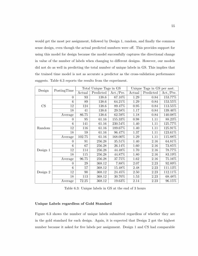
55

would get the most per assignment, followed by Design 1, random, and finally the common

sense design, even though the actual predicted numbers were off. This provides support for

using this model for design because the model successfully captures the directional change

in value of the number of labels when changing to different designs. However, our models

did not do as well in predicting the total number of unique labels in GS. This implies that

the trained time model is not as accurate a predictor as the cross-validation performance

suggests. Table 6.3 reports the results from the experiment.

Design PostingTimeTotal Unique Tags in GS Unique Tags in GS per asst.

Actual Predicted Act./Pre. Actual Predicted Act./Pre.

CS

0 93 138.6 67.10% 1.29 0.84 153.77%6 89 138.6 64.21% 1.29 0.84 153.55%

12 124 138.6 89.47% 0.95 0.84 113.55%18 41 138.6 29.58% 1.17 0.84 139.46%

Average 86.75 138.6 62.59% 1.18 0.84 140.08%

Random

0 95 61.16 155.33% 0.98 1.11 88.23%6 141 61.16 230.54% 1.40 1.11 125.77%

12 116 61.16 189.67% 1.40 1.11 125.91%18 59 61.16 96.47% 1.37 1.11 123.61%

Average 102.75 61.16 168.00% 1.29 1.11 115.88%

Design 1

0 91 256.28 35.51% 1.40 2.16 64.81%6 67 256.28 26.14% 1.60 2.16 73.85%

12 114 256.28 44.48% 1.70 2.16 78.77%18 115 256.28 44.87% 1.80 2.16 83.19%

Average 96.75 256.28 37.75% 1.62 2.16 75.16%

Design 2

0 29 368.12 7.88% 2.07 2.23 92.89%6 57 368.12 15.48% 2.48 2.23 111.13%

12 90 368.12 24.45% 2.50 2.23 112.11%18 113 368.12 30.70% 1.53 2.23 68.48%

Average 72.25 368.12 19.63% 2.14 2.23 96.15%

Table 6.3: Unique labels in GS at the end of 3 hours

Unique Labels regardless of Gold Standard

Figure 6.3 shows the number of unique labels submitted regardless of whether they are

in the gold standard for each design. Again, it is expected that Design 2 got the highest

number because it asked for five labels per assignment. Design 1 and CS had comparable

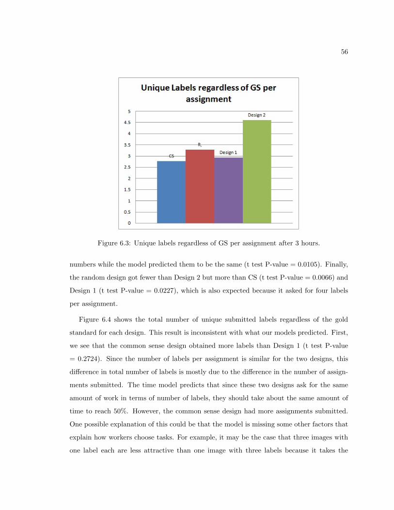
56

Figure 6.3: Unique labels regardless of GS per assignment after 3 hours.

numbers while the model predicted them to be the same (t test P-value = 0.0105). Finally,

the random design got fewer than Design 2 but more than CS (t test P-value = 0.0066) and

Design 1 (t test P-value = 0.0227), which is also expected because it asked for four labels

per assignment.

Figure 6.4 shows the total number of unique submitted labels regardless of the gold

standard for each design. This result is inconsistent with what our models predicted. First,

we see that the common sense design obtained more labels than Design 1 (t test P-value

= 0.2724). Since the number of labels per assignment is similar for the two designs, this

difference in total number of labels is mostly due to the difference in the number of assign-

ments submitted. The time model predicts that since these two designs ask for the same

amount of work in terms of number of labels, they should take about the same amount of

time to reach 50%. However, the common sense design had more assignments submitted.

One possible explanation of this could be that the model is missing some other factors that

explain how workers choose tasks. For example, it may be the case that three images with

one label each are less attractive than one image with three labels because it takes the

57

Figure 6.4: Total Unique labels regardless of GS after 3 hours.

workers more effort to look at different images and reposition their minds in the new image.

Design 2 had the least unique labels submitted. Again, this is due to the low number of

submitted assignments and the inaccuracy of the time model. The result for the random

design is also inconsistent with the model’s prediction. This is also because of the number

of submitted assignments are so much higher than what the model predicted. Together

with the under-prediction for the other designs, the number of unique labels for the random

design ended up being the most out of all. Table 6.4 includes all the data on unique labels.

Conclusion

Based on the trained models for predicting behavior within and outside the HIT, I formu-

lated two optimization problems for each of the goals discussed. After seeing the initial

solutions to the problems and the unrealistic amount of work asked for in each HIT in the

chosen designs, I further constrained the solution space by requiring the amount of pay per

label to be above a minimum threshold. I ran experiments with the two selected designs,

together with a common sense design and a random design as benchmarks for comparison.

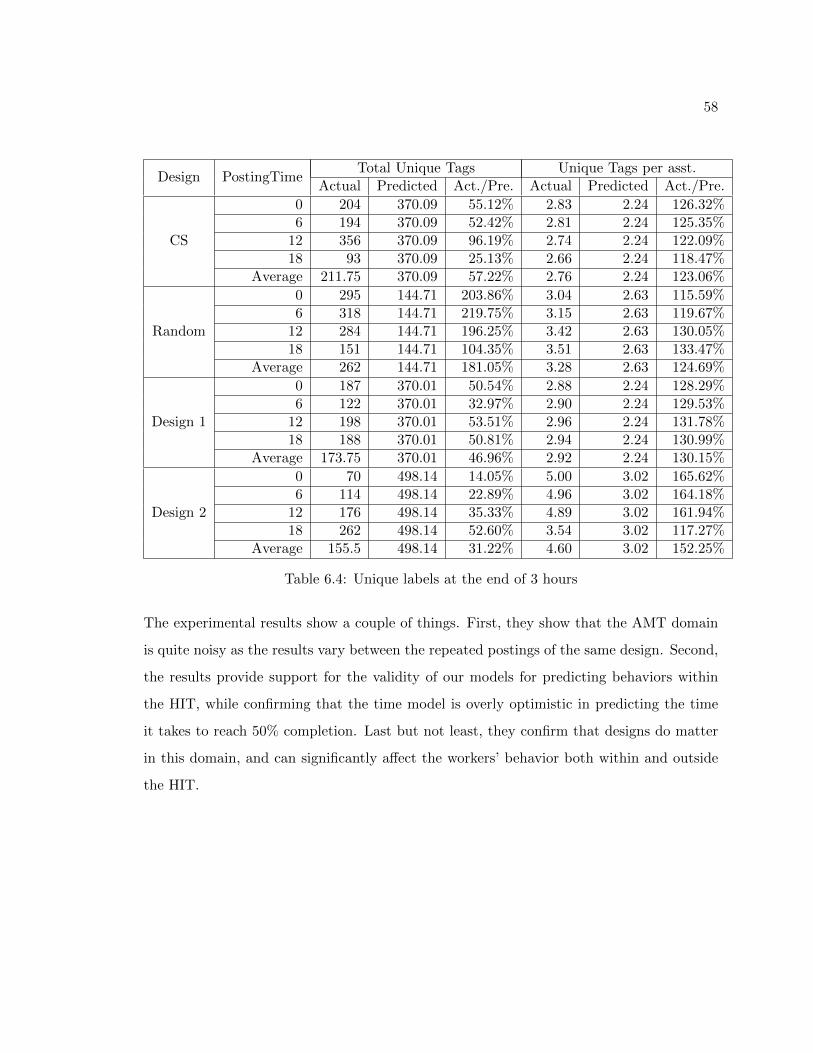
58

Design PostingTimeTotal Unique Tags Unique Tags per asst.

Actual Predicted Act./Pre. Actual Predicted Act./Pre.

CS

0 204 370.09 55.12% 2.83 2.24 126.32%6 194 370.09 52.42% 2.81 2.24 125.35%

12 356 370.09 96.19% 2.74 2.24 122.09%18 93 370.09 25.13% 2.66 2.24 118.47%

Average 211.75 370.09 57.22% 2.76 2.24 123.06%

Random

0 295 144.71 203.86% 3.04 2.63 115.59%6 318 144.71 219.75% 3.15 2.63 119.67%

12 284 144.71 196.25% 3.42 2.63 130.05%18 151 144.71 104.35% 3.51 2.63 133.47%

Average 262 144.71 181.05% 3.28 2.63 124.69%

Design 1

0 187 370.01 50.54% 2.88 2.24 128.29%6 122 370.01 32.97% 2.90 2.24 129.53%

12 198 370.01 53.51% 2.96 2.24 131.78%18 188 370.01 50.81% 2.94 2.24 130.99%

Average 173.75 370.01 46.96% 2.92 2.24 130.15%

Design 2

0 70 498.14 14.05% 5.00 3.02 165.62%6 114 498.14 22.89% 4.96 3.02 164.18%

12 176 498.14 35.33% 4.89 3.02 161.94%18 262 498.14 52.60% 3.54 3.02 117.27%

Average 155.5 498.14 31.22% 4.60 3.02 152.25%

Table 6.4: Unique labels at the end of 3 hours

The experimental results show a couple of things. First, they show that the AMT domain

is quite noisy as the results vary between the repeated postings of the same design. Second,

the results provide support for the validity of our models for predicting behaviors within

the HIT, while confirming that the time model is overly optimistic in predicting the time

it takes to reach 50% completion. Last but not least, they confirm that designs do matter

in this domain, and can significantly affect the workers’ behavior both within and outside

the HIT.

Chapter 7

Conclusion

In this thesis, I study the problem of goal-oriented task design in the domain of Amazon

Mechanical Turk. This problem is important because we can imagine workers on the AMT

system responding differently to different tasks, in terms of how the task is structured,

how much work is in a task, and how much the requester is paying per task. We can see

these factors influencing the tasks workers choose to work on and the results they submit.

Specifically, this work studies the design of image labeling tasks on AMT. Even though this

work is focused on a specific type of task, with some modifications, the approach to the

problem could very well be applied to other types of task, or even other domains.

7.1 Brief Review

In Chapter 1, I introduced the problem of goal-oriented task design on AMT and why it

is important. I gave an overview of image labeling tasks, and the approach to solve this

problem. I presented some potential obstacles and situated this problem in the contexts

of related works on AMT, designs on AMT, image labeling and environment design. In

Chapter 2, I gave an overview of the AMT domain, a specific description of image labeling

tasks, and why I chose image labeling tasks to work with. I presented the two design goals

in which a requester may be interested. In Chapter 3, I formulated the design problem for

59

60

image labeling tasks on AMT. I presented an overview of the idea of environment design

and why its idea of designing based on knowledge learned from observations is particular

suitable for our problem. Then, I provided a sketch of our design approach. In Chapter 4, I

introduced the mathematical models for describing the workers’ behavior both within and

outside the HIT. I listed the potential important factors for the models and described the

intuitions behind choosing them. In Chapter 5, I discussed the results of the initial experi-

ment. I used the experimental data to train the models proposed in Chapter 4, and based

on cross-validation results, selected the ones I use to design. In Chapter 6, I formulated the

two design problems using the selected models, and ran experiments to assess the validity of

the models. The experimental results show that the models for predicting behavior within

the HIT are somewhat accurate, while the time model for predicting behavior outside the

HIT is overly optimistic.

7.2 Future Work

This work opens up several questions for future work:

• Machine learning techniques. Are there more suitable machine learning techniques

for this domain? Can we more accurately predict the workers’ behavior? Are there

automatic methods for extracting important features?

• Active learning. Can we apply active learning to this domain? Instead of running an

initial batch of experiments to obtain training data, are there methods that automat-

ically pick configurations that allow the model to learn the most?

• General behavior model. Can we learn a general model for describing how workers

behave? Instead of learning specific models for each metric of an interested goal, can

we learn a generative model that applies to different types of tasks and goals?

• Applications to other domains. Can we generalize the method used in this work to a

general framework for automatic task design, not just in AMT?

61

7.3 Conclusion

In this thesis, I developed a method to automatically design image labeling tasks on Amazon

Mechanical Turk, drawing techniques from machine learning and ideas from environment

design. I built a software framework using AMT’s API to conduct experiments on the

system. The experimental results confirmed the importance of design in this domain and

added support for the validity of our trained models. This work provides a foundation for

applying a quantitative approach to design in the real-world domains.

Bibliography

[1] Amazon. http://amazon.com/.

[2] Lydia B. Chilton, Clayton T. Sims, Max Goldman, Greg Little, and Robert C. Miller.

Seaweed: a web application for designing economic games. In In Proceedings of the

ACM SIGKDD Workshop on Human Computation, pages 34–35, Paris, France, 2009.

[3] ESP dataset. http://www.cs.cmu.edu/ biglou/resources/.

[4] Jia Deng, Wei Dong, Richard Socher, Li-Jia Li, Kai Li, and Li Fei-Fei. Imagenet: A

large-scale hierarchical image database. In In the 2009 IEEE Conference on Computer

Vision and Pattern Recognition, pages 248–255, 2009.

[5] Mark Everingham, Luc Van Gool, Christopher K.I. Williams, John Winn, and An-

drew Zisserman. The pascal visual object classes challenge 2008 (voc2008) results.

http://www.pascal-network.org/ challenges/voc/voc2008/workshop/.

[6] Li Fei-Fei, Rob Fergus, and Pietro Perona. One-shot leraning of object categories. IEEE

Transactions on Pattern Analysis and Machine Intelligence, 28 no. 4, April 2006.

[7] Gregory Griffin, Alex Holub, and Pietro Perona. Caltech-256 object category dataset.

Technical Report, 2007.

[8] Weka 3: Machine Learning Software in Java. http://www.cs.waikato.ac.nz/ml/weka/.

[9] Munir Kotadia. Google image index hits 1 billion mark. http://news.cnet.com/google-

image-index-hits-1-billion-mark/2100-1024 3-5567523.html/.

62

63

[10] Google Image Labeler. http://images.google.com/imagelabeler/.

[11] Winter Mason and Duncan J. Watts. Financial incentives and the ”Performance of

Crowds”. In In KDD-HCOMP ’09, Paris, France, June 2009.

[12] Turker Nation. http://turkers.proboards.com/.

[13] Bryan C. Russel, Antonio Torralba, Kevin P. Murphy, and William T. Freeman. La-

belme: a database and web-based tool for image annotation. International Journal of

Computer Vision, 77 (1-3):157–173, May 2008.

[14] Erick Schonfeld. Who has the most photos of them all?

http://techcrunch.com/2009/04/07/who-has-the-most-photos-of-them-all-hint-it-

is-not-facebook/.

[15] J. Shotton, J. Winn, C. Rother, and A. Criminisi. Textonboost: Joint appearance,

shape and context modeling for multi-class object recognition and segmentation. In In

ECCV, pages 1–15, 2006.

[16] Rion Snow, Brendan O’Connor, Daniel Jurafsky, and Andrew Y. Ng. Cheap and fast

- but is it good? evaluating non-expert annotations for natural language tasks. In

In the 2008 Conference on Empirical Methods in Natural Language Processing, pages

254–263, Honolulu, October 2008.

[17] Alexander Sorokin and David Forsyth. Utility data annotation with amazon mechanical

turk. In In the Computer Vision and Pattern Recognition Workshops, January 2008.

[18] Qi Su, Dmitry Pavlov, Jyh-Herng Chou, and Wendell C. Baker. Internet-scale collection

of human-reviewed data. In In the 2007 International World Wide Web Conference,

Banff, Alberta, Canada, May 2007.

[19] Antonio Torralba, Rob Fergus, and William T. Freeman. 80 million tiny images: a

large dataset for non-parametric object and scene recognition. IEEE Transactions on

Pattern Analysis and Machine Intelligence, 30 no. 11, May 2008.

64

[20] Amazon Mechanical Turk. http://mturk.com/.

[21] Turkit. http://groups.csail.mit.edu/uid/turkit/.

[22] Turkopticon. http://turkopticon.differenceengines.com/.

[23] Luis von Ahn and Laura Dabbish. Labeling images with a computer game. In In ACM

SIGCHI Conference on Human Factors in Computing Systems, 2004.

[24] Man-Ching Yuen, Ling-Jyh Chen, and Irwin King. A survey of human computation

systems. In In the 2009 International Conference on Computational Science and En-

gineering, 2009.

[25] Haoqi Zhang, Yiling Chen, and David C. Parkes. A general approach to environment

design with one agent. In In the 21st International Joint Conference on Artificial

Intelligence (IJCAI-09), Pasadena, CA, 2009.

[26] Haoqi Zhang and David C. Parkes. Enabling environment design via active indirect

elicitation. In In the 4th Multidisciplinary Workshop on Advances in Preference Han-

dling, Chicago, IL, 2008.

[27] Haoqi Zhang and David C. Parkes. Value-based policy teaching with active indirect

elicitation. In In the 23rd AAAI Conference on Artificial Intelligence (AAAI’08),

Chicago, IL, 2008.

[28] Haoqi Zhang, David C. Parkes, and Yiling Chen. Policy teaching through reward

function learning. In In the 10th ACM Electronic Commerce Conference (EC’09),

Stanford, CA, 2009.

Automatic Task Design on Amazon Mechanical...

Documents

Transcript of Automatic Task Design on Amazon Mechanical...