AUTOMATIC RECTIFICATION OF LANDSAT IMAGES USING FEATURES DERIVED FROM DIGITAL TERRAIN MODELS

by

JAMES J . LITTLE

A.B. HARVARD UNIVERSITY 1972

A THESIS SUBMITTED IN PARTIAL FULFILLMENT OF THE REQUIREMENTS FOR THE DEGREE OF

MASTER OF SCIENCE

i n

THE FACULTY OF GRADUATE STUDIES

(Department of Computer Science)

We accept t h i s thesis as conforming to the required standard.

THE UNIVERSITY OF BRITISH COLUMBIA

July , 1980

(c) James J . L i t t l e , 1980

I n p r e s e n t i n g t h i s t h e s i s i n p a r t i a l f u l f i l m e n t o f t h e r e q u i r e m e n t s f o r

a n a d v a n c e d d e g r e e a t t h e U n i v e r s i t y o f B r i t i s h C o l u m b i a , I a g r e e t h a t

t h e L i b r a r y s h a l l make i t f r e e l y a v a i l a b l e f o r r e f e r e n c e a n d s t u d y .

I f u r t h e r a g r e e t h a t p e r m i s s i o n f o r e x t e n s i v e c o p y i n g o f t h i s t h e s i s

f o r s c h o l a r l y p u r p o s e s may be g r a n t e d by t h e Head o f my D e p a r t m e n t o r

by h i s r e p r e s e n t a t i v e s . I t i s u n d e r s t o o d t h a t c o p y i n g o r p u b l i c a t i o n

o f t h i s t h e s i s f o r f i n a n c i a l g a i n s h a l l n o t be a l l o w e d w i t h o u t my

w r i t t e n p e r m i s s i o n .

D e p a r t m e n t o f .

The U n i v e r s i t y o f B r i t i s h C o l u m b i a 2075 W e s b r o o k P l a c e V a n c o u v e r , C a n a d a V6T 1W5

D E - 6 B P 7 5 - 5 1 1 E

i i <

/ABSTRACT

Before two images of the same object can be compared, they must be brought into correspondence with some reference datum. This process i s termed r e g i s t r a t i o n . The reference can be one of the images, a synthetic image, a map or other symbolic representation of the area imaged. A novel method i s presented for automatically determining the transformation to ali g n a Landsat image to a d i g i t a l t e r r a i n model, a structure which represents the topography of an area. Parameters of an affi n e transformation are computed from the correspondence between features of t e r r a i n derived from the d i g i t a l t e r r a i n model, and brightness d i s c o n t i n u i t i e s extracted from the Landsat image.

i i i

Table of Contents

1. Introduction 1 2. Previous Work 9

2.1 Registration and Rectification 9 2.2 Digital Terrain Models 12 2.3 Synthetic Images 14 2.3.1 Reflectance Functions 14 2.3.2 Sun Position 18 2.4 Feature Selection 18 2.5 Matching 20 2.5.1 Symbolic Matching 21 2.5.2 Geometrically Constrained Matching 23

3. The Registration Method 28 3.1 The F i r s t Stage: Feature Extraction 28 3.1.1 Extracting Features from Digital Terrain Models 28 3.1.2 Extracting Features from the Landsat Image 29 3.1.3 Selecting Feature Points 31 3.1.4 Line Growing 35 3.1.5 Approximations to Lines 36 3.2 The Second Stage: Matching 44 3.3 The Affine Transformation 46 3.4 Construction of a Pairing 49 3. 5 Support for a Pairing 53 3.6 Consistency of the Transform 56 3.7 Verification 56

4. Implementation and Testing 59 4.1 The Input 59 4.2 Programming Languages 60 4.3 Data Structures 60 4.4 Estimating the Affine Transform 62 4.5 Examples of Registration and Results 63

5. Discussion and Conclusions 74 5.1 Discussion 74 5.2 Further Work 76 5.3 Conclusions 76

Bibliography 77

L i s t of Figures

Figure 1 Subsection of a Land sat image 3 Figure 2 Contour p l o t (100 meter interval) of the d i g i t a l t e r r a i n model .. 4 Figure 3 Landsat features 5 Figure 4 DTM features 6 Figure 5 Registered Landsat image 8 Figure 6 Triangulated Irregular Network 13 Figure 7 The geometry of l i g h t r e f l e c t i o n 16 Figure 8 Synthetic image 17 Figure 9 Sun position i n terms of azimuth and elevation 19 Figure 10 Self-shadowed facets 30 Figure 11 Subsection of a Landsat image 32 Figure 12 Output of the edge detection step 33 Figure 13 Edge detector output after echo suppression 34 Figure 14 Lines before merging 37 Figure 15 Compatibility of segment directions i n l i n e merging 38 Figure 16 Lines after merging 39 Figure 17 Line generalization 40 Figure 18 Varying the d e t a i l l e v e l i n generalization 42 Figure 19 The band of a curve 43 Figure 20 Landsat features 45 Figure 21 Structured and simple ridges 47 Figure 22 Close f i t i n a p a i r i n g 51 Figure 23 Loose f i t i n a pairing 52 Figure 24 Mismatches and support 54 Figure 25 Self-consistency of a transform 57 Figure 26 Synthetic image for September 14 1976 64 Figure 27 DTM features with matched points 65 Figure 28 Landsat features with matched points 67 Figure 29 Subsection of Landsat image 68 Figure 30 Synthetic image for January 8 1979 70 Figure 31 DTM features with matched points 71 Figure 32 Landsat features with matched points 72 Figure 33 Registered Landsat image for January 8 1979 73

V

Acknowledgement

I sincerely thank my supervisor Robert J . Woodham for his help. His perceptive c r i t i c i s m of my work i n progress has not only improved t h i s thesis but also has been very b e n e f i c i a l to my education. I also wish to thank Alan K. Mackworth for encouraging me o r i g i n a l l y bo pursue t h i s thesis topic.

1

1. Introduction

There are many image analysis tasks where the objects i n the scene are

known beforehand. Often i n d u s t r i a l inspection and manipulation tasks

involve determining the position and orientation of a known part within a

given image (Hsieh and Fu,1979; Agin,1980; Myers, 1980). S i m i l a r l y ,

biomedical applications, such as chest X-ray interpretation (Ballard et a l . ,

1979), often deal with images whose general content i s known. The

interpretation of images acquired v i a s a t e l l i t e or a e r i a l photography i s

f a c i l i t a t e d by knowledge of the scene given i n form of maps and other

geographic data. Once the position and orientation of objects i n a scene i s

determined, image analysis s i m p l i f i e s . Thus, registering the image to the

scene model i s an important f i r s t step i n automatic image interpretation.

In remote sensing, the s p a t i a l relations between the objects i n the scene

are precisely known, and the geometric r e l a t i o n between image and scene

model can be characterized by a fixed mathematical transformation of known

form but unknown parameters. In contrast, the number of r i b s i n a chest

x-ray, for example, i s given, as we l l as t h e i r general s p a t i a l

relationships, but the i r precise size and position are not precisely known.

The importance of re g i s t r a t i o n has been demonstrated i n the domain of

Landsat images. When a new image has been brought into correspondence with

surface data, the interpretation of ground cover i s improved. For example,

the e f f e c t of shading due bo variations i n surface topography and shadows

can be estimated (Woodham, 1980). Thus f a r , r e g i s t r a t i o n has eluded

complete automation. The object of t h i s thesis i s to present a method for

automated r e g i s t r a t i o n of Landsat images.

A Landsat MSS image measures scene radiance i n each of four spectral

2

bands, at a nominal ground resolution of 79 x 79 meters. The position and

attitude of the Landsat MSS platform i s known with li m i t e d precision. After

systematic corrections based on the estimated platform position and

attitude, the ground location of an image point may d i f f e r from i t s true

position by as much as 10 kilometers. Since each picture element (pixel) of

a Landsat MSS image has a nominal ground spacing of 56 meters i n the across

track d i r e c t i o n and 79 meters i n the along track d i r e c t i o n , t h i s represents

an error of up to 179 p i x e l s . Further processing i s thus required to relate

the image coordinate system to other coordinate systems.

A d i g i t a l t e r r a i n model (DTM) represents surface elevation as a

function of ground coordinates. A DTM can be accurately located i n a

geographic coordinate system. A Landsat image registered to a d i g i t a l

t e r r a i n model can be d i r e c t l y compared with other sources of geographic

information, and other images.

An automatic method for registering Landsat images to d i g i t a l t e r r a i n

models i s developed. As an example, figure 1 shows a 100 x 100 section of a

Landsat image. Figure 2 shows a contour p l o t at 100 meter int e r v a l s of the

d i g i t a l t e r r a i n model. In the method presented here, a set of c u r v i l i n e a r

features i s determined from both the Landsat image and the DTM. Features

from the Landsat image are shown i n figure 3 while those selected from the

DTM are depicted i n figure 4 . A correspondence between the elements of the

two sets of c u r v i l i n e a r features i s established which s a t i s f i e s both

geometric (shape) constraints and topological (adjacency) constraints. The

matching between elements determines point pairs input to a least-squares

estimator for the parameters of an affine transform. The image re g i s t r a t i o n

problem i s transformed into the problem of matching sets of curves i n the

plane. The points on the features used for calculating the transform are

Figure 1 100 x 100 pixe l subsection of Landsat image (band 7) from September 14,1976, frame ID 11514-17153. Photographed from screen of COMTAL Vision 1.

4

5

6

Figure 4 Features derived from DTM using the sun's position at the time of image acquisition on September 14, 1976.

7

labelled 1-6 i n figures 3 and 4. The registered Landsat image i s shown i n

figure 5 . The derived a f f i n e transform i s :

x' = a x + b y + c y 1 = d x + e y + f

where (x,y) are Landsat image coordinates, (x',y') are DIM coordinates, and

where

a = 0.555292 b = 0.131612 c = 1.944259 d = -0.143495 e = 0.7736 12 f = 2.197464

Chapter 2 reviews previous work i n r e g i s t r a t i o n , feature detection,

d i g i t a l t e r r a i n models and matching methods.

Chapter 3 develops the method for registering images to d i g i t a l t e r r a i n

models. Knowledge of sun position i s used to select features for

re g i s t r a t i o n . Geometric constraints are used to guide the re g i s t r a t i o n

process.

Chapter 4 presents the pa r t i c u l a r implementation used to r e a l i z e the

method.

Chapter 5 discusses the results and t h e i r relevance to other image

understanding tasks.

8

Figure 5 Registered Landsat image for September 14, 1976. The white square o u t l i n e s the 10 kilometer area covered by the DTM. Photographed from the screen of the COMTAL Vi s i o n 1.

9

2. Previous Work

2.1 Registration and R e c t i f i c a t i o n

Image reg i s t r a t i o n i s the process of determining the correspondence

between elements of two or more images and applying a transformation to one

image to a l i g n i t with the other. Two s a t e l l i t e images would f i r s t be

registered i n order bo proceed with change detection. However, i t i s often

necessary to register images not just to each other but also to absolute

ground coordinates. Registering an image to absolute ground coordinates i s

ca l l e d image r e c t i f i c a t i o n . Often the term re g i s t r a t i o n i s used for both

image-to-image r e g i s t r a t i o n and image-bo-ground r e g i s t r a t i o n ( i . e . ,

r e c t i f i c a t i o n ) .

Commonly, two images are registered by manually selecting ground

control points (GCP's) from each image (Bernstein, 1976). A ground control

point i s a d i s t i n c t i v e ground feature detectable i n an image. Typical GCP's

are a i r p o r t s , land-water boundaries, f i e l d patterns and highway

intersections. Parameters of an appropriate transformation are calculated

from a subset of the selected GCP's. For each GCP i n one of the images, the

corresponding GCP must be located i n the second. Manual selection of GCP's

i s time-consuming. Several techniques have been developed to automate

p a r t i a l l y the selection of ground control points.

As an i n i t i a l improvement to the manual method, correla t i o n techniques

can be used to improve the estimates of the GCP locations. For each GCP i n

the reference image, a small m x n subsection of image surrounding the GCP

i s used as a template. The best matched position of the template determines

10

the location of the corresponding GCP. The best position is that at which

the correlation of the template with the image is maximized. The

correlation between an m x n template SI and a subsection of an image S2 at

(x,y) is:

YL Z_Sl(i,j) • S2(x+i,yfj)

High output of this operation may result i f one of the subsections has a

high average gray level. For this and other reasons, i t is convenient to

normalize the correlation, resulting in the following formulation: Vw. y\

/ / (Sl(i,j) - Si) • (S2(x+i,y+j) - S2)

<r~~ 2 I— (Sl(i,j) - Si) 7 / (S2(x+i,y+j) - S2)

where r-*'*-

sT=l/(m-n)£ L Sl(i,j) and

S2 = l/(m.n)^_ y 1 "s2(x+i,y+j)

Then a perfect correlation corresponds to a value of 1. Sequential

similarity detection algorithms (SSDA's) can be used to speed up template

matching (Barnea and Silverman,1972). This correlation process is repeated

for each GCP. The refined GCP locations are used to determine the

parameters of the registration transformation. This refinement technique

can be embodied in a fully automatic registration procedure i f a library of

GCP templates is maintained for use in the registration of subsequent images

of the same area.

The GCP method can be further automated by introducing automatic

selection of the GCP's. As a first step toward this, the reference image

can be regularly subdivided into overlapping subimages, each of which is

11

used as a template i n the correlation technique. This automatic method has

d i f f i c u l t i e s . There i s no guarantee, for example, that the GCP templates

can be located by correlation i n other images. The GCP's produced by-

regular subdivision are random with respect to the content of the image.

Davis and Kenue(1977) describe a method for automatically selecting ground

control points i n a reference image. Ground control points are selected

where there i s a strong connected set of brightness d i s c o n t i n u i t i e s . The

algorithm thresholds the gradient of the image and finds connected sets of

pix e l s i n the thresholded gradient image. GCP's are selected from the

resulting set so as to be as evenly scattered about the image as possible.

This method improves upon regular subdivision of the reference image into

templates, but i t also suffers two major shortcomings:

1) Since the GCP's are chosen on the basis of image features, the GCP's have no necessary r e l a t i o n bo ground features whose appearance can be expected bo remain constant i n other images. 2) In p a r t i c u l a r , no attempt i s made to take account of possible changes i n illumination between the images, which w i l l systematically a f f e c t the appearance of the templates.

In the absence of a scene model, not much more can be done. However,

d i g i t a l t e r r a i n models, when available, can be used to select and v e r i f y

GCP's for r e g i s t r a t i o n .

Horn and Bachman (1978) use synthetic images generated from d i g i t a l

t e r r a i n models to register Landsat images. The synthetic image represents

the appearance of the t e r r a i n under the illumination conditions

corresponding to the sun position at the time of image acquisition. Their

published work assumes that the transformation between the synthetic image

and the Landsat image can be described i n terms of rotation, translation and

scale change. A correlation of the r e a l and synthetic images i s used as

measure of goodness of f i t to guide the adjustment of rotation, translation

and scaling. The correlation of the entire image i s ultimately used. This

12

i s computationally expensive. The authors avoid some of t h i s expense by

f i r s t using low resolution images to produce rough estimates of the

transformation parameters. The f u l l resolution of the data i s used to

compute the f i n a l refinements to the transformation parameters.

The method presented i n t h i s thesis follows the s p i r i t of the work of

Horn and Bachman. The known position of the sun i s used to predict the

t e r r a i n features which w i l l appear as d i s t i n c t image features. The symbolic

features themselves are used to determine the transformation parameters.

2.2 D i g i t a l Terrain Models

A d i g i t a l t e r r a i n model (DTM) represents the surface of the earth i n a

p a r t i c u l a r region. This i s usually taken to mean that the DTM can be used

to determine the elevation of the surface at any point i n the region.

Besides providing height information, a d i g i t a l t e r r a i n model also

represents the surface orientation since slope and aspect can be derived.

Slope information i s c r u c i a l for accurate calculation of the synthetic

image. Because the DTM i s defined i n a ground coordinate system, an image

registered to a DTM can be d i r e c t l y compared to other sources of geographic

information.

A common representation of t e r r a i n i s as a discrete g r i d of t e r r a i n

elevations. Slope i s determined i n a g r i d representation by l o c a l

differencing. A l t e r n a t i v e l y , t e r r a i n can be modelled as a set of contiguous

non-overlapping triangular facets (figure 6), i n a Triangulated Irregular

Network (TIN) (Peucker et a l . , 1978). In the TIN, slope information i s

d i r e c t l y computed from the surface facets. E f f i c i e n t procedures e x i s t for

converting the g r i d to a TIN and vice-versa (Peucker et a l . , 1978; Fowler

Figure 6 A Triangulated Irregular Network (TIN)

14

and L i t t l e , 1979). The d i g i t a l t e r r a i n model used for the work described

herein was constructed i n the TIN format.

The structure of t e r r a i n can be modelled by the network of ridges and

channels (divides and streams). The ridges are convex l i n e a r surface

features which, t h e o r e t i c a l l y , connect passes (saddle points) bo peaks

(relative maxima). In practice the set of ridges on a surface also includes

convex line a r features which connect to the main ridges that do j o i n passes

to peaks. Channels are concave line a r features connecting passes to p i t s

(relative minima). In addition, the surface behavior of the t e r r a i n between

ridges and channels i s modelled. This surface behavior includes l i n e s along

which the surface changes slope. These are termed breaks of slope. Actual

production of a DTM, whether a g r i d or a TIN, often involves recording the

t e r r a i n structure of ridges and channels.

Several methods e x i s t for deriving the the location of ridges and

channels from the g r i d representation (Peucker and Douglas, 1975; Toriwaki

and Fukumaru,1978). The TIN model i s advantageous for feature selection

since ridges, channels and breaks of slope are e x p l i c i t l y represented as the

boundaries of triangular facets.

2.3 Synthetic Images

2.3.1 Reflectance Functions

Image irradiance at a given point depends on the object material imaged

at that point and i t s orientation i n space with respect to the l i g h t

source (s) and viewer. Following Horn and Bachman, one model of image

15

formation uses a surface reflectance function:

PHI(I,E,G) = P * CDS(I)

where I, E, and G are the incident angle(I), emittance angle(E), and the

phase angle (G) (figure 7). In the above equation, P i s an albedo factor

depending on the surface composition, which, without additional a p r i o r i

knowledge, i s assumed to be constant. This reflectance function models a

lambertian surface which, as a perfect d i f f u s e r , appears equally bright from

a l l viewing directions. The incident angle(I) i s the angle between the

surface normal and the illumination d i r e c t i o n . In the case of Landsat

imagery, the p r i n c i p a l l i g h t source i s the distant sun, so that the

illumination d i r e c t i o n i s e f f e c t i v e l y constant for a l l surface points.

Diffuse illumination from the atmosphere and possibly from other scene

elements i s ignored i n the synthetic image.

The DTM provides accurate estimates of the surface orientation for the

test area. A synthetic image i s produced under the assumption of an

orthographic projection and a single l i g h t source at the known sun position.

The brightness i n the synthetic image at each picture element (pixel) i s a

function of the surface orientation at the appropriate point i n the DTM.

Figure 8 shows a synthetic image produced from a d i g i t a l t e r r a i n model,

using the simple reflectance function described above, with the sun from the

northwest at 45 degrees elevation, as i n standard cartographic convention.

16

Figure 7 The geometry of l i g h t r e f l e c t i o n from a surface element i s governed' by the incident angle, I, the emittance angle, E, and the phase angle, G. (after Horn and Bachman, 1978)

17

Figure 8 Synthetic image of the DTM. The ligh t source i s positioned in the northwest at 4 5 degree elevation, as in cartographic convention. Photographed from the screen of the OOMTAL Vision !.

18

2.3.2 Sun Position

In order to produce a synthetic image corresponding to an actual

imaging s i t u a t i o n , i t i s necessary to determine the sun's pos i t i o n at the

precise time of image acquisition. Fortunately, the time of acquisition of

each Landsat scan l i n e i s accurately determined and recorded as part of the

image annotation data. Standard tables or formulae can be employed to

determine the position of the sun at a given date, time, l a t i t u d e and

longitude. Sun position i s described i n terms of azimuth, the angle of

rotation about the v e r t i c a l axis, i n degrees clockwise from north, and

elevation, the angle of rotation above the horizontal (figure 9) . In t h i s

description, standard cartographic convention situates the l i g h t source at

azimuth 315 degrees, elevation 45 degrees.

2.4 Feature Selection

The l i t e r a t u r e i n image analysis abounds with techniques for

determining the po s i t i o n and orientation of brightness d i s c o n t i n u i t i e s i n

images (Davis, 1975). /An operator which performs t h i s task i s c a l l e d an

"edge detector". Generally, edge detectors perform w e l l i n locating sharp

boundaries where the r e l a t i v e brightness difference i s large and the

boundary i s l o c a l l y l i n e a r . For the purpose of the method presented i n t h i s

thesis, the features to be found i n Landsat images are r e s t r i c t e d to

d i s c o n t i n u i t i e s between r e l a t i v e l y bright and dark regions. The i n t e n s i t y

differences between regions are known to be large and the tra n s i t i o n s

between the regions sharp. The focus of the research i s not on the design

19

Figure 9 Definition of the position of the sun in terras of azimuth 0 , and elevation (j> .

20

of an optimal f i l t e r for detecting such features. Rather i t i s assumed that

most edge-detecting operators w i l l be robust enough to detect the required

boundaries.

S i m i l a r l y , the choice of method for joining p i x e l s which display edge

a c t i v i t y into l i n e s i s not c r i t i c a l . Portions of the image features sought

w i l l be r e l a t i v e l y straight, and connecting these into curves i s

straightforward, toy rule for connection which prefers extending e x i s t i n g

l i n e s along the general l i n e tendency i s acceptable. I t i s presumed when

the features are used that there w i l l be gaps i n the curves, so the degree

to which a line-growing method i s able bo bridge these gaps i s not c r i t i c a l .

In sum, feature selection techniques were chosen from e x i s t i n g methods i n

the l i t e r a t u r e .

Feature selection i n the domain of the d i g i t a l t e r r a i n model derives

from an investigation of the production of synthetic images (discussed i n

section 2.3). The method for DTM feature selection w i l l be elaborated i n

section 3.1.1.

2.5 Matching

In the automatic r e g i s t r a t i o n method presented i n the thesis, a

one-to-one correspondence i s derived between symbolic features of an image

and a d i g i t a l t e r r a i n model. This correspondence between features can be

modelled as a matching of the features, depending upon the s i m i l a r i t y of

their descriptions. I f the matching between features based on thei r

symbolic descriptions i s r e l i a b l e , then matching methods can be used for

automatic r e g i s t r a t i o n . Other researchers have considered the problem of

matching an image to a model of the scene. Research on matching

21

descriptions of an image to models of the scene can be divided into those

which handle symbolic descriptions only, and those which also manipulate

geometric relat i o n s . The topics of interest i n t h i s work are both

representations of object and image relations and the control structures

used i n matching.

2.5.1 Symbolic Matching

Barrow and Popplestone (1971) describe the adjacency r e l a t i o n of

picture regions by a region adjacency graph (RAG). This graph i s

necessarily planar. A description of a model scene i s also represented i n

terms of a RAG. Recognition of elements i n the picture i s performed by

matching a region with a model oomponent. Both region adjacency graphs are

augmented by edges indicating relations between regions such as r e l a t i v e

s i z e , position (above-below, l e f t - r i g h t ) , shape and convexity. The match i s

incrementally increased, one region at a time. The search space can be

represented as a tree; nodes represent matchings and descendants of a node

represent developments of the matching at the node by adding another region.

The search space i s probed for a solution using b e s t - f i r s t search.

Barrow and B u r s t a l l (1976) use maximal matching of graphs for matching

r e l a t i o n a l structures, such as image and scene descriptions represented as

graphs. A graph i s defined as a set N of nodes, and a r e l a t i o n R, a subset

of NxN. A matching from GI to G2 i s a subset S of NlxN2 which preserves the

relations i n each graph; for a l l pairs (a,A) and (b,B) i n S, a i s connected

to b i n GI i f and only i f A i s connected to B i n G2. A matching i s maximal

when no other matching has higher c a r d i n a l i t y . Under t h i s d e f i n i t i o n , a

node i n GI may be matched to more than one node i n G2 and vice versa. Two

22

pairs are 'compatible' i f the pairs are in S. A graph is derived, as

follows: the elements of the graph (the set X) are elements of S and the

relation (H) between elements of the graph i s that of compatibility between

pairs. Given a graph so constructed, a maximal matching of the original

graphs can be obtained by finding a maximal clique(complete subgraph) of

(X,H). It is clear that in such a clique a l l pairs are compatible, by

definition, and that i t s order is maximal. If the restriction that a = b

i f f A = B i s added to the definition of compatibility, the correspondence

generated by the maximal matching i s one-to-one. To our dismay, however,

this merely reduces a d i f f i c u l t problem to an NP-complete problem. However,

the best clique-finding algorithms seem to perform e f f i c i e n t l y in most

cases.

Tanimoto (1976) offers an excellent discussion of the motivation for

using graph matching and develops an algorithm for enumerating a l l maximal

matchings of two graphs. A matching assigns labels to regions in the

segmentation of an image. The labels form one set of nodes in a bipartite

graph, and the regions the other set. Edges represent the compatibility of

descriptions of a region with a label and hence restricted to a yes-no

decision. A maximal matching of the bipartite graph so formed i s the

maximal set of edges from one set of nodes to the other, where a node occurs

at most in one edge. Tanimoto notes that methods for constructing such

bipartite graphs are 'neither usually obvious nor necessarily possible'.

One approach i s to allow edges which satisfy many constraints such as degree

restrictions. Usually these are determined by local constraints, that i s ,

those which only require examining the neighbors of a node. A maximal

matching can be generated in 0{e * sqrt(n)) time, where e is the number of

edges in the graph, and n the number of nodes. An algorithm i s presented by

23

Tanimoto which can l i s t the set of maximal matchings of the graph. A note

of caution: the number of maximal matchings i s p o t e n t i a l l y exponential i n n.

A recent paper by I t a i , Rodeh and Tanimoto (1978) also characterizes the

cases when matching problems with r e s t r i c t i o n s are NP-complete (Aho et

al.,1974), and provides a discussion of the a p p l i c a b i l i t y of graph-matching

v i s - a - v i s constraint propagation.

Maximal matching techniques are appealing because once the

compatibility r e l a t i o n i s constructed, generation of matchings i s e f f i c i e n t .

However, the effectiveness of maximal matching methods depends upon the

extent to which the compatibility r e l a t i o n can constrain matchings to

appropriate ones. I f the compatibility r e l a t i o n i s too general, many

matchings w i l l be generated which are incorrect. Computing compatibility

becomes expensive when the i n t e r r e l a t i o n of features extends more than just

to l o c a l features. In the re g i s t r a t i o n problem, i n p a r t i c u l a r , the solution

must s a t i s f y global constraints, while compatibility testing must be rather

l o c a l to allow maximal matching to be a successful alternative method. In

addition, i t i s not clear that the relations among features can e a s i l y be

characterized by descriptions such as ' l e f t - r i g h t ' or 'near-far'. Rather,

metric relations such as angle and distance are appropriate i n t h i s domain,

especially as they are precisely known for the DTM. Using metric relations

becomes more important when matchings between i n t r i n s i c aspects of features,

such as shape, length or position, are less r e l i a b l e .

2.5.2 Geometrically Constrained Matching

Fischler and Eschlanger (1973) d e t a i l a method for matching a reference

image i n raster format to a reference image which i s described by a graph

24

composed of components (coherent pieces of the model). For each of these

components, a l o c a l evaluation array (LEA) i s computed. The LEA measures

the goodness of f i t of each component of the model at each point i n the

image, rather l i k e the goodness of f i t of a template at a l l points i n the

image. The model components are assumed to be joined together by springs.

The cost of a matching i s the amount of tension i n the springs j o i n i n g the

"components. This method i s compatible with a 'rubber-sheeting*

transformation of the image, i n which d i r e c t i o n i s not g l o b a l l y preserved

and scaling can vary across the image.

Dynamic programming i s used to solve the matching problem. Using the

LEA, the cost of orienting the constituent component subassemblies can be

computed, recorded i n tabular form, and used to f i n d a global minimum cost

matching. The cost of t h i s method increases exponentially as the degree of

interconnection of the components r i s e s . As an alternative, the authors

suggested an incremental method, very similar to Barrow and Popplestone's

technique. The work i s of note i n two respects: f i r s t , i t constructs a f u l l

transformation from one image to the other, and second, i t uses geometric

constraints as w e l l as semantic constraints i n the matching. The

re g i s t r a t i o n method presented i n t h i s thesis uses an incremental method.

Bajcsy and Chance (1975) studied the problem of establishing the

correspondence between images of brain s l i c e s before and after chemical or

physical operations i n which there i s appreciable shape d i s t o r t i o n of the

brain. The images are processed to extract the veins i n the images. The

nodes (vein junctions) are ordered by degree. A matching i s generated by

comparing the degree of junctions from the two images. Because i t i s l i k e l y

that an edge i n one graph w i l l show up i n another, t h i s seems an appropriate

strategy. The graphs are not t o t a l l y matched i n t h i s process; rather, the

25

i n i t i a l matching i s used as a 'seed' to a r e g i s t r a t i o n procedure which

perturbs the i n i t i a l mapping s l i g h t l y i n order to reach an optimal match.

The authors state that without such an i n i t i a l match, the h i l l - c l i m b i n g

method of the r e g i s t r a t i o n i s not s u f f i c i e n t l y constrained and might 'walk

o f f the edge of the image'.

Work at SRI (Bolles et a l . , 1979) models the transformation from the

test image to the reference as a function of camera parameters, such as

f o c a l length, position, yaw, pitch and r o l l . The reference i s a 'database'

of highways and features of highways. An essential part of the SRI method

i s that there i s a good 'a p r i o r i ' estimate of the camera parameters and of

the errors i n these parameters. These estimates are used to predict the

location and extent of the region i n the image which i s to be searched for

an element from the reference image. The predicted search region for an 0

element i s termed i t s 'uncertainty region'. "Once an element i s located

within i t s search region, the search regions for other elements are

constrained i n location and siz e . The pairing of reference element and

image element provides new information which i s used to improve the camera

parameters and reduce the errors. Both line a r and point features are

hand-selected from the reference image for r e g i s t r a t i o n . Because highway

structures, such as the boundaries of lanes, are l o c a l l y very s i m i l a r , i t i s

possible to mistake a feature for one o f f s e t from the proper match. To

prevent t h i s s i t u a t i o n , the system i d e n t i f i e s features nearby which can be

used to v e r i f y a match, and searches for them i n the image. For example,

highways are composed of several p a r a l l e l lanes; i n detection of a highway

the system searches for l o c a l l y o f f s e t lanes to confirm the matching of

others. This notion i s termed ' l o c a l support' for a feature match. The

matching of elements provides information for the correspondence refinement

26

process which solves the nonlinear camera parameter estimation problem.

Bolles (1979) describes a further use of the maximal clique method for

matching features i n an image with a model. Nodes i n the feature graph

represent l a b e l l i n g s of nodes. /Arcs represent compatibility relations

between the l a b e l l i n g s of features. These relations are based on distance

and orientation measures computed i n the image and compared with model

descriptions. A maximal clique i n t h i s graph represents a maximal match of

the features of the image with the labels i n the model. As with a l l maximal

matching methods, there are d i f f i c u l t i e s with the combinatorial behavior of

the problem and the inordinate size of the graphs; generating graphs for

reasonable problems i n i t s e l f i s time-consuming. Bolles (p. 144) suggests

several ways of improving the method:

1) R e s t r i c t the model to key features

2) Use geometric l i m i t s with respect bo some feature to exclude

unnecessary features.

3) I t e r a t i v e l y apply the maximal clique method to refine the

assignment.

With respect bo the l a s t point, Bolles further states "the benefit of t h i s

approach i s derived from the fact that the st r u c t u r a l constraints are

applied sequentially instead of a l l at once" (p.145).

In general, methods for maximal matching suffer from the d i f f i c u l t i e s

encountered i n Bolles*s method. E x p l i c i t construction of the relations

which may hold between elements of the model and the features of the image

i s i t s e l f an expensive task. The re g i s t r a t i o n method presented here follows

the s p i r i t of Bolles's work. The method depends upon an analysis of the

27

model to f i n d promising features of the model. These are found i n the

image. Nearby features of the model are used to confirm the i n i t i a l

matching. Then additional features are selected for matching, from the

r e s t r i c t e d set constrained by the previous matches. Local support for a

feature acts as a breadth-first look-ahead to select promising matches,

following which a depth-first search i s conducted for further matches. In

addition, once an estimate for the matching has been constructed, i t i s

l o c a l l y adjusted to improve the r e g i s t r a t i o n .

These facets of the method anticipate the suggestions of Bolles. The

illumination conditions at the time of image acquisition are used to

determine the features. Key features are selected based on the s t r u c t u r a l

complexity of t h e i r components. The geometric constraints of the transform

derivation guide i t s development. Lastly, the inspection and rejection of

choices at early stages of the search deliver the benefits of sequential

exploration of the p o s s i b i l i t i e s .

3. The Registration Method

The r e g i s t r a t i o n method proceeds i n several stages. The data consist

of the raw Landsat image and a d i g i t a l t e r r a i n model (DIM) for the area

imaged. The time at which the image was acquired i s known. In the f i r s t

stage, features of the d i g i t a l t e r r a i n model and the Landsat image are

derived. The second stage considers matchings of three features from both

the DTM and the image. Each match determines the parameters of an a f f i n e

transformation. When one of the derived transforms predicts other

ridge-to-Landsat feature pairings, with a s u f f i c i e n t l y small t o t a l residual

error, the transformation i s accepted. Otherwise, r e g i s t r a t i o n f a i l s .

3.1 The F i r s t Stage; Feature Extraction

3.1.1 Extracting Features from D i g i t a l Terrain Models

Since the sun's position corresponding to the Landsat image i s known,

i t i s possible bo determine the location of convex breaks of slope which

w i l l appear i n the image with strong brightness d i s c o n t i n u i t i e s , as follows:

The slope of each surface facet i s derived and the brightness of the facet

determined using the reflectance function. For every location i n the TIN

where surface slope changes (represented by the junction of facets), the

brightness of the surface facets adjoining i s computed. The difference

between these values indicates the r e l a t i v e magnitude of the brightness

discontinuity to be expected at that position. In testing the method, only

those edges are selected which are bounded, on one side, by a self-shadowed

29

facet (one which receives no d i r e c t illumination), and, on the other side,

by a facet whose predicted brightness i s r e l a t i v e l y high (figure 10) . This

r e s t r i c t s the features to a small subset of a l l edges which w i l l generate

brightness d i s c o n t i n u i t i e s . Many ridges w i l l not be self-shadowed on one

side, but w i l l nevertheless appear as sharp d i s c o n t i n u i t i e s i n the image.

However, areas i n self-shadow, i f present, w i l l be very dark i n the image,

and t h e i r appearance w i l l be less sensitive to ground cover v a r i a t i o n .

Self-shadowed ridges tend to l i e perpendicular to the azimuthal d i r e c t i o n of

the sun. This leads to strong constraint along the d i r e c t i o n p a r a l l e l to

the azimuthal d i r e c t i o n of the sun, but l i t t l e constraint i n the orthogonal

di r e c t i o n . Pairings of features at junctions or endpoints of features

provide the needed constraint i n the orthogonal d i r e c t i o n . Edges s a t i s f y i n g

t h i s c r i t e r i o n are merged into curves when their endpoints are adjacent and

merging them does not cause the resulting curve to loop back upon i t s e l f .

Only those curves are output which represent a strong brightness

discontinuity. These curves w i l l be termed "ridges" i n the following

discussion of the re g i s t r a t i o n method, while noting that the curves can be

generated both by t e r r a i n ridges as w e l l as other convex breaks of slope.

The features extracted from the DTM are shown i n figure 4.

3.1.2 Extracting Features from the Landsat Image

In the Landsat image, some surface slope breaks appear as boundaries at

transitions between bright and dark regions. Desirable boundaries are those

formed by convex breaks of slope oriented perpendicular to the azimuthal

di r e c t i o n of the sun's illumination. Shadow boundaries also appear as

transitions between bright and dark regions, but, since the d i r e c t i o n of the

30

Figure 10 Self-shadowed sur faces.

31

incident illumination i s known, they can be distinguished from the

t r a n s i t i o n features formed by ridges. Shadows are dark on the side o f the

edge nearer the l i g h t source. Figure 11 shows the Landsat image subsection

used for the r e g i s t r a t i o n tests.

3.1.3 Selecting Feature Points

The Landsat image i s correlated with an edge detector composed of two

orthogonal components. The 5x5 Sobel operator (Iannino and Shapiro, 1979)

was used because i t had been reported to y i e l d acceptable re s u l t s , i n the

l i t e r a t u r e . The r a t i o of the outputs of the components of the operator

provides an estimate of the dir e c t i o n of the boundary element passing

through the p i x e l s tested.

The edge detector gives high values not only at d i s c o n t i n u i t i e s , but

also at p i x e l s o f f s e t from the d i s c o n t i n u i t i e s . This produces secondary

l i n e s , c a l l e d echos, l y i n g p a r a l l e l to the o r i g i n a l (figure 12). In order

to eliminate these as early as possible a scheme of Nevatia and Babu (1979)

i s used, to edge element i s judged to e x i s t at a p i x e l i f :

a) the magnitude of the f i l t e r output i s above a threshold b) i t s magnitude i s higher than that of i t s two neighbors i n the d i r e c t i o n normal to the estimated edge d i r e c t i o n , and c) the edge directions of these neighboring p i x e l s are within 45 degrees of the d i r e c t i o n at the central p i x e l .

I f any of these conditions do not hold then no edge element i s judged to

e x i s t . The e f f e c t of t h i s process i s to suppress the echo elements at an

ea r l y stage, eliminating the need for l a t e r curve thinning procedures

(figure 13).

32

33

******* ****

* ***** ** ******** ** ************ ******************* ********************* ********************* ******** ** ********** ** ******** *** ** *************** ***************** ****

*** **** ***

*** ***

*** ***** ****** ***** **** * *** **

** *** **** ****** ***** ******** ***** ************ * ************ ****** ** ******** ****** ***** ****** ***** ************** ************ ***************** *********** ***** ********* *** *** *

********* **** ******* ** ******* **** ***** ****** *** *****

* * * * * * *

* * * * * * * * * * *

* * * f * *

*** ***** ***************** *************** ************

** **** ***

*** * * ** **** ****** ****** ****** ******** ********* ************ ************ ********** ******** ********

*** ***** ****** ******* ****** *** ***** ******** ************** ****************

***** ********* **** ** ***** ****** ********* *********** ************ ****** *** ****** ******* ******** ********* ********* ******* ******

********************************* ******************************** ************ ********************** * ******* ******************** *** ****** *************************** ***** ********************** ******** ********* ******** ************* ****** ******* ********** ****** ********** ******** *** *********

************ ************** * ****************************** ***** ********* ****************** **** ** ******** ********************** **** ********** **************** ****** **** . ******** *********************** ** * ******* ** ******** ***********

** **** * * *** *** ******* **** ******* *** ****** * ****** *** *** ********** * ***** ***** * ***** **** * ***** ** "**** **** ****

* ******** *** ** ******* ******* **** * ***** ******* * **************** ********************* ******************** ********************* ********************** ******************** ************ ******** ************* ****** ************** ******* ** *********************** ******************************* ****************************** **************************** * **************************** ***************************** *************************** ***************************** ********** ******************* ****************************** **** ************* ** ******* *** ******* ******* ******

**** ****** ****** ****** ******* ****** ****** ****** • ******* ******* ******* ******* ***** *** ***

*** **

*** ***

*** *****

***** ******** **** ************ ******, * *****

****** ***** ** **

********** *********** *********

*****

*** *** *** ****

**** *****

******** ***********

****** ***** *

***** * ***** *

****** * ******** **.

********* *** *********

*********** ************

**************** **************** * **************** **** *********** **** *** *

*********** *** ******* * ********************** ***** ***** ************************ ****************** **** ******** ****************** ****** **** * ********* ** ****** ******* ****** ****** ********** ***** ** *************** * ********* *******

*******

** ********************* * ***************** *******. ******************* ** ********************** *** ***************** **** ***** ************ ****** **** ****** *********** ********* ******** ****** *********** ********** ****************** ***** ******************* *****. ******************** *** ***** *********** ** ***** ***

******* ******

**** ' ***** *******

********** *******

****** *******

** *** ****** *** ** ********* ** *** *********** **** ************ ***** * *********** **************** ** ** **

************ ********** ************* *********** ****************** ****************** ******** **** * ********** ** ** ************ * ***************** ** ***************************** ************ *************** ******************* ************ *************** ******************** ***************** ** ***************** *** ************** ************************ **

*********** *********** ******** ****** * **** ***********

******** ********* ********* ********** *********** *** ************** * **** ************

* ********** ******************* **** ******************** ***** ************************ **************************************

** ************** *** *********** ****************** *** **** *********

************' *** ****

**** ****

***+ *********** *** **** **** * **** +** *****

** . ********** ************* * ****************************** ******************************

*********************** ********* ********** ******* **** **** *** * *** ***** * ****** ***** ****** *********** ******* ******** ******* ******** **** *********

****** *** *** ** ********** • *** ** ********

***

****** ******* *** **** ******* ******* -********* ************ . ***************

** ***

***

********** • *** ** *** *********** ***

*** **** *************** ************** ************** ************** ***************** **** ************************************ ******** ************************** ********* ******* ******************** *************** •

****************** ****** ********************* ***************** *****************^ ************ ******************

J.*i*J.J.J.XJ.J.J.J.J.iJ.J.J.J.J.̂ ********** **** ************* ******** ** *******************

***** ******* *******

************************************* *** ************* ******************

********** ********** *** ********* ******** ******** ********* ********* **** ************ * . : . - • -. * * * * * * * * * * *

********* * ******* ***** ** **** **

Figure 12 i

Result of applying the edge detector. **s represent edge elements whose o r i e n t a t i o n i s consistent with the sun's posi t i o n .

34

***** ********* **

*** ***

**** ***

*** ***

*** *** *** ** ****

** **

**** ****

** ******

** *** ** *** * ** **

*** *** ** *** *** ******* ***

***

** ** * *

*** ** * * ** ** **

* ** **

**** ***

** ****** *** * ****

* ** ** ****

* ** ***********

*** * **

** ** * *** * * *

***** *** ***** * ****

** * ** ****** *** *

*** **

*** ** *** **

*** .***

*** *** .** ** * * *

** ** . ** ** ** *** *** ***** . *

*** **

************ ******** ***** * ***** *

* ****** **

*** ********** ***** * ** **** * * *** ** **

** ** '** **

* * * * ** *

** .

* *** ***

Figure 13 Edge detector output after echo suppression.

35

3.1.4 Line Growing

The output of the Sobel operator i s used to construct the line a r

features, following the method of (Bajcsy and Tavakoli, 1976). The process

i s divided into two steps. F i r s t , p i x e l s are connected into curves

represented as sets of p i x e l s . Next, a piecewise l i n e a r approximation i s

derived for these curves, and curves are merged when possible. In the

discussion which follows, the terms " l i n e " and "curve" w i l l be used

interchangeably to refer to a s t r i n g of points connected by st r a i g h t l i n e

segments.

In the f i r s t stage, a histogram of the values of the f i l t e r output i s

derived. This density histogram i s used to d i r e c t the process so that l i n e s

are 'grown1 from those points which had the highest output from the

f i l t e r i n g step. A cumulative d i s t r i b u t i o n function i s derived from the

density histogram. At each step i n the l i n e growing process, the threshold

i s relaxed so that f i v e percent more p i x e l s are above i t . I n i t i a l l y the

threshold i s set at the 95 percent l e v e l .

At each stage i n the l i n e construction process, the threshold i s set at

the proper l e v e l and a l l points i n the image above the threshold and not

already i n a l i n e are processed. The threshold i s then lowered a l e v e l , and

the process repeated, u n t i l the minimum l e v e l i s reached. Lines are

constructed incrementally i n t h i s f i r s t stage; at f i r s t a l i n e consists of a

single point. When an adjacent point l i e s above the current threshold, and

cannot be joined to any e x i s t i n g l i n e , i t i s joined to the single point and

forms a two-point l i n e . To ensure that the l i n e s found have less than a

certain maximum curvature, points are added to an e x i s t i n g l i n e only i f they

are adjacent to the endpoints of the l i n e and the segment connecting the new

36

point to the endpoint l i e s within 45 degrees of the d i r e c t i o n of the nearest

segment i n the l i n e .

The r e s u l t of the f i r s t stage i s a set of l i n e s each consisting of a

set of connected p i x e l s . Figure 14 shows these l i n e s ; at each p i x e l the

l a s t d i g i t of the curve to which that p i x e l belongs i s printed. In the next

stage, these l i n e s are merged into larger connected l i n e s when two

conditions hold: f i r s t , the l i n e s are adjacent at t h e i r endpoints, and,

second, the segment directions are compatible, that i s , j o i n i n g the two

l i n e s at the i r endpoints does not cause the resulting curve to loop back

upon i t s e l f . The segments are compatible i n d i r e c t i o n i f the dot product o f

the segments, considered as vectors or i g i n a t i n g at the common endpoint, i s

less than or equal to zero (figure 15). Figure 16 shows the curves after

merging. To aid i n curve merging, a piecewise line a r approximation i s

derived for each of the curves.

3.1.5 Approximations to Lines

A piecewise l i n e a r approximation to a d i g i t a l l i n e (Ranter, 1972;

P a v l i d i s , 1977) approximates a l i n e to a given precision by a set of l i n e a r

segments connecting points on the l i n e . In i t s construction, the f i r s t and

l a s t points i n the l i n e are connected by a straight l i n e segment. The

extreme points l y i n g farthest i n perpendicular distance from the l i n e

segment are determined, B and D i n the example shown i n figure 17 . The

extreme points are included i n the approximation i f t h e i r distances from the

segment are above the specified threshold, which w i l l be termed the " d e t a i l

l e v e l " of the l i n e . The l i n e i s then subdivided into the three sets of

points to the l e f t , between and rig h t of the selected points. The three

37

o 05

60 1 1 1 6

7 166 I , 71 J 2 11

,3 8 2 918 9 „ 1 8 990 8 1 9 8 49

5 0 1 9 449 5 1 6

7222 22

223 24

524 252

25 825

222 9 7777 20

73 888 3

184 3 J

6 3 3

9

0 0

90 75 19 75 666

„i9 7 5 666 J 9 75 2 09 75

0 77 7

7 17 7.

72 37 7

88 89

89 8

84

8884

884 0 988

11111 015

28 28

2 24 4

11

98 98

66661"" 777 go 8

8888 57 2 91 39

8 81 8 8

15 3 44 8 6657 15 93 8 1 666 69 8

„?, 2 8

09 7 8 0 8

01 01

701 3 00

5 8 22 56 77 3 88

56 435 8 9 0000 4

555 04

29 29

220 324

55555

11

9

5 1 9 3

i 2

F i g u r e 1 4

L i n e s b e f o r e m e r g i n g . T h e d i g i t a t e a c h p i x e l i s t h e l a s t d i g i t o f t h e n u m b e r o f t h e l i n e t o w h i c h t h e p i x e l b e l o n g s .

38

compatible segments

incompatible segments

Figure 15 Two l i n e s can be merged i f the dot product of the segments at the j o i n point i s negative.

39

o 05 6

10 f>

666 8 76 8 2 66

1 8 2 668 1 8 668 1 8 660

0 1 9 8 66 5 0 1 9 666 5 1 6

7666 -66

663 64

664 6 266 6 26

8 2 6 2 2 2 9

8888 20 9 8 3

888 3 184 3 8 35 8 1

0 °

l8° il" 222 10 75 222

0 0 75 2 3

0°° T 7 7 5

} 7 5555 7 2 e5,5

37 59 7 59

7 5 7 54 7 554

955 0 95

11111 9 5 015 9 5

11111 777 „ 55 1111 57 2 5 1

11 35 H r t 5 1 55

11 5 5 0 1 554

11 55555 15 8 44 8 5557

15 88 8 1 6 6 6 68 8

8 28 88 7 8

8 8 8 1

8 1 7 8 1 3

88 8 4

5 8 22 56 77 2 88 9

5 6 225 8 9 2 2 2 2 2

555 22 8 8 1 „

8 11 8 • • " • : . • • • . . . . • „ • . - • :

9 2 9

2 2 3 2 2 . 3

2 4 2 ,

3 2 4

F i g u r e 1 6

L i n e s a f t e r m e r g i n g . T h e d i g i t a t e a c h p i x e l i s t h e l a s t d i g i t o f t h e n u m b e r o f t h e l i n e t o w h i c h t h e p i x e l b e l o n g s .

40

F i g u r e 1 7

A c u r v e a n d t h e t r e e r e p r e s e n t a t i o n o f i t s g e n e r a l i z e d f o r m .

41

subsets of the l i n e are processed recursively i n a similar fashion. In

figure 17, these subsets are TAB, BCD and DEF. I f the point farthest from

the segment i n a p a r t i c u l a r subset i s within the threshold distance, then

processing of that subset of the l i n e i s stopped, and only the endpoints of

the l i n e segment retained. The process of finding such an approximation i s

termed 'generalization'. The t r e e - l i k e structure derived i n t h i s fashion i s

useful i n cartographic computations (Ballard,1979). A tree for a

generalized form of a curve i s also shown i n figure 17.

By varying the d e t a i l l e v e l used i n computing the curve approximation,

a family of approximations i s generated (figure 18) . A l t e r n a t i v e l y , the

perpendicular distance of a point i n the curve from the next highest l e v e l

segment can be recorded i n the approximation. The distance so found i s a

measure of the significance of that point i n the approximation of the curve.

By constructing two l i n e s , p a r a l l e l to and o f f s e t from a given segment

of a curve, and at a given perpendicular distance, a region i n the plane i s

described which i s c a l l e d the 'band' of that segment of the curve. When the

segment connects the endpoints of the curve, the region i s the band of the

curve (figure 19). The d e t a i l at which the curve i s examined can be varied

by a l t e r i n g the perpendicular distance at which the band i s constructed.

The band of a curve w i l l be used to determine whether a curve overlaps

another, i n curve comparison and i n testing of the r e g i s t r a t i o n .

Since most of the l i n e s i n the Landsat image contain many colinear

points, the l i n e approximations contain s i g n i f i c a n t l y fewer points than the .

the o r i g i n a l l i n e s represented as connected sets of p i x e l s . Using the

approximations, d i r e c t i o n a l decisions involving the orientation of l i n e

segments are less affected by perturbations at the end of curves caused by

quantization. The output of the feature-detector i s the set of l i n e s i n

42

F i g u r e 1 8

V a r y i n g t h e d e t a i l l e v e l i n g e n e r a l i z a t i o n . T h e d o t t e d l i n e s r e p r e s e n t t h e g e n e r a l i z e d f o r m o f t h e c u r v e a t e a c h l e v e l .

Figure 19 The band of a curve.

44

generalized form, which are longer than a specified minimum length (figure

20). These cu r v i l i n e a r features derived from a Landsat image w i l l be termed

"l-edges".

Since the ridges are derived from the TIN representation, they are

represented as a s t r i n g of contiguous l i n e segments. I t i s natural to

convert t h i s form to the piecewise lin e a r approximations used for curves

found i n the Landsat image. I f a DTM feature i s represented by a single

straight l i n e segment, then i t i s 'simple'. Any curve whose representation

includes i n t e r i o r points i s said to be 'structured*. The ridges and l-edges

are input to the second stage.

3.2 The Second Stage; Matching

The basic approach i n the second stage i s to locate the known features,

the ridges, i n the image. Features are located sequentially, and the

location of a feature i n an image w i l l constrain search for other features.

Ridges w i l l be located by s t r u c t u r a l l y matching ridges with l-edges. A

ridge matched to an 1-edge i s a "pairing". A pairing locates a ridge i n the

image and provides a pair of matched points which are used as ground control

points (section 3.4). Because of the sequential nature of the algorithm, i t

i s useful to introduce an ordering.

The ridges are considered i n the order of thei r s t r u c t u r a l complexity.

This i s because i t i s assumed that the more strongly an element d i f f e r s from

a straight l i n e the less l i k e l y i t i s to be matched incorrectly. The goal

of the matching process i s to pair a s u f f i c i e n t number of ridges and l-edges

to compute transform parameters. Features i n the DTM are ordered as

follows:

45

F i g u r e 2 0

L a n d s a t i m a g e f e a t u r e s f o r s u b s e c t i o n i n f i g u r e s 1 1 - 1 6 .

46

1. M l structured ridges are considered before simple ridges (figure 21). 2. The strength of a ridge i s the product of i t s length and the estimated brightness discontinuity across i t . Structured ridges and simple ridges are each ordered according to the ridge strength.

The r e l a t i o n of structured feature to structured feature i s p o t e n t i a l l y

a many-to-many r e l a t i o n . A portion of a ridge may be represented by two or

more l i n e segments while the corresponding 1-edge i s represented as a single

l i n e segment, or vice versa. To consider a l l possible relations between two

structured curves means examining the relations between a l l powersets of

both. Representing and manipulating such relations s i g n i f i c a n t l y

complicates curve matching. Consequently, a l l structured features i n the

landsat image are broken down into simple elements, represented by single

l i n e segments.

3.3 The Affine Transformation

Horn and Woodham (1979) demonstrate that, i f small, second-order

ef f e c t s are ignored, an aff i n e transformation i s s u f f i c i e n t to register

small subsections of a Landsat image to a plane tangent to the earth's

surface. The parameters of t h i s transformation can be expressed i n terms of

the parameters of the s a t e l l i t e ' s o r b i t and other fixed quantities. An

aff i n e transform has 6 degrees of freedom and can be written as:

x' = a x + b y + c

y ' = d x + e y + f

where x,y are image coordinates and x',y' are DTM coordinates. A subset of

47

F i g u r e 21

S t r u c t u r e d ( A ) a n d s i m p l e ( B ) r i d g e s .

48

a f f i n e transformations can be expressed as a composition of rotation,

translation and scaling of the coordinate axes. However, the f u l l y general

affine transform does not admit t h i s simple decomposition.

Finding the tranformation parameters requires at least three matched

points. These can be determined manually by ide n t i f y i n g ground control

points i n both the DTM and the image. Let the coordinates of the image

points be ( X j , y t ) , (x^,y 2) and (x^y^) and the DTM coordinates be (x ,y ( ),

( x 2 ,y ) and ( x } , y 3 ) . Then

x, y, 1 a d x . y i x l Y i 1 • b e — x 3 y 3 l c f

so -1 a d b e c f

x, y» 1 x i Y t 1

/ /

X V

I f more than three GCP's are supplied, a least-squares estimate of the

transform can be computed. I f

M

x» y, i x z y z l

V n 1

Then the least-squares estimate with equal weighting to a l l points for the

transform parameters i s :

a d b e c f

T - « T (M-M) • M

x,» y.i y*

X.

Once three feature pairings have been established, the affi n e transform

can be estimated. A set of three pairings w i l l be termed a 'matching' and a

set of more than three pairings an 'extended matching'. Exhaustive

49

examination of a l l matchings i s too expensive. The number of t r i p l e s grows

as n . Hence the number of matchings grows as n , where each of the feature

sets i s of c a r d i n a l i t y n. Knowledge of the constraints imposed on the

problem i s used bo l i m i t the search space. An estimate of the a f f i n e

transform i s derived (following Horn and Woodham, 1979) from o r b i t a l

parameters included i n the image annotation, and other fixed parameters of

the scanner. Section 4.4 presents the analytic expressions for the

parameters of the a f f i n e transform and describes the parameters of the

s a t e l l i t e o r b i t . Because t h i s estimate of the transform i s available, i t

can be used bo eliminate the generation of some incorrect matchings.

3.4 Construction of a Pairing

I n i t i a l l y , the location of an image feature i n the DTM i s known only to

within 10 kilometers. This delimits a search region for a feature. The

system begins by selecting a ridge and finding the l-edges i n i t s search

region. Each 1-edge i s transformed according to the 'a p r i o r i ' transform

estimate, and compared with the candidate ridge. The basis of the

comparison i s the representation of a curve as a piecewise l i n e a r curve.

The construction of t h i s representation, as described i n section 3.1.5,

involves determination of the d i r e c t i o n of the curve, which i s the d i r e c t i o n

of the vector connecting i t s endpoints. The band about the curve i s a

region i n the plane bounded by two l i n e s p a r a l l e l bo the d i r e c t i o n vector

and o f f s e t from i t by a fixed amount. The width of the band i s the distance

between the p a r a l l e l l i n e s . Assessment of a pairing of features proceeds as

follows:

50

a) I f the ridge i s simple, the transformed 1-edge i s translated so that one of i t s endpoints coincides with an endpoint of the ridge segment. The perpendicular distance D from the ridge to the other endpoint of the 1-edge i s computed. There are three cases:

1) D i s less than or equal to the band width. The positions at which the 1-edge can be matched include a l l points i n the ridge segment. In practice, three positions are used (figure 22): at either endpoint, or at the centerpoints, the averages of the endpoints of the segments. 2) D i s less than twice the band width. The 1-edge i s constrained to match i t s centerpoint to the centerpoint of the ridge (figure 23). 3) Otherwise, the pairing i s rejected.

In cases 1 and 2, the measure of goodness of the match i s the cosine of the angle between the two curves. In case 3, the measure of the match i s a r b i t r a r i l y set to 0. The translation vector for the pairing i s constructed from the difference of the matched points.

b) I f the ridge feature i s structured, then the 1-edge i s compared with each of the l i n e segments i n the ridge as above. The r e s u l t of the comparison i s a l i s t of matchings of the 1-edge with each of the segments i n the ridge.

I f structured l-edges were used i n pairing development, endpoint matches

could be confirmed on the basis of the r e l a t i v e orientation of the segments

meeting at that endpoint. Local context i s provided by the adjacency of

segments. In the present system, l o c a l support for a pairing serves t h i s

purpose.

The r e s u l t of a match determines a point-to-point correspondence which

i s used i n estimating the a f f i n e transform. The l i s t of pairings of ridge

and l-edges, sorted by value, i s associated with the ridge. Pairings whose

value i s too small are not allowed to enter into the construction of a

matching. This acts to eliminate pairings which can only arise from

combinations of rotation, scaling and skewing inconsistent with the known

imaging geometry.

51

Figure 22 Close f i t i n a p a i r i n g , with the three matching p o s i t i o n s .

52

53

3.5 Support for a Pairing

A p a i r i n g s p e c i f i e s a translation vector. The residual error i n

position of an image feature after transformation can be modeled as a

translation. Hence the translation needed bo bring a transformed 1-edge

inbo correspondence with a ridge i s used to guide the development of

matchings. Each subsequent pai r i n g must be consistent with the previous

pairings, that i s , the translation required to construct the pairing must be

similar to those previous. S i m i l a r i t y between translation vectors i s

measured by treating each translation as a point i n the plane and finding

the distance between the points. I f the distance i s too large, the

translations are incompatible. Otherwise, the translations are considered

consistent. Testing translation consistency eliminates the generation of

many incorrect matchings.

Experimentation with the feature sets has shown that translation alone

i s not a s u f f i c i e n t constraint. For example, the location and orientation

of ridges i s often controlled by the underlying geological structure of the

region. Ridges are often p a r a l l e l or nearly so, and the spacing between

ridges can be very regular. Hence, a pairing of a ridge to an image feature

may be correct i n orientation, but o f f s e t by the inter-ridge spacing.

Consider the following example: The problem i s to register the image

resembling the numeral 4 represented i n figure 24 to a model of the numeral.

Image segments are referred to by t h e i r endpoints, ABCDEF, and the model

segments by the same l e t t e r s , with quotes, A'B'C'D'E'F'. In t h i s example,

i f segment A-C i s compared with B-D, the match w i l l be high i n value,

assuming an i d e n t i t y a p r i o r i transformation. Orientation and length of the

segment do l i t t l e bo distinguish A-C and B-D. To eliminate incorrect

B

0 — E

F

a)

A. Bi A iB

/ i

D! E C

i /

Figure 24 An image (1), i t s model (2), and a mis-match demonstrate support for a matching.

55

matchings cause by t h i s phenomenon, the l o c a l s p a t i a l structure of both the

ridges and the 1-edges must be used to guide the matching. In terms of the

example, note that when A-C i s registered to B'-D', C-D overlaps D*-E',

p a r t i a l l y confirming the match with B'-D'. But when A-C i s paired with

A'-C1, a l l segments i n the image w i l l p a r t i c i p a t e i n a pairing consistent

with that involving A-C.

When an i n i t i a l p a i r i n g of features i s made, nearby ridges are examined

and a t a l l y i s kept of the number of nearby ridges which can be paired with

1-edges i n a matching consistent with that under construction. Consistency

here i s again measured by comparing the translations necessary to bring a

feature into alignment, under the a p r i o r i transform, with a given 1-edge.

I f a structured ridge i s being considered, the t a l l y i s formed by counting

the number of segments i n the ridge which can be paired with 1-edges under

mutually compatible translations. Developing a pa i r i n g o f the elements of a

structured ridge with several simple 1-edges compensates somewhat for the

decomposition of structured 1-edges into separate simple features. The

simple 1-edges can be paired with the elements of a structured ridge as they

would have been had they s t i l l been joined i n a structured 1-edge. The

pairings of ridge and 1-edges are ordered by the number of supporting

pairings, ( i . e . , by the extent to which they can be l o c a l l y extended). This

strategy can be understood as a generalization of the scheme of determining

l o c a l support for lin e a r features employed i n the SRI system (Bolles et a l . ,

1979).

At t h i s point, a feature (whole or part) i s matched to a 1-edge, and a

set of compatible pairings has been generated. Each of the elements i n t h i s

set i s i n turn selected as the second pairing for the matching. By

selecting other ridges with translation-compatible pairings as the t h i r d

56

part of the match, the matching i s extended to include three mutually

translation-consistent pairings of features. With the s i x values from the

matching, an affi n e transform can be determined. Each pairing of a ridge

and an 1-edge provides a point-to-point match for the parameter

determination.

3.6 Consistency o f the Transform

When an affi n e transform i s determined for a set of three point

pairings, the resulting transform w i l l predict the points with no error.

Hence i t i s necessary also to test how the transform predicts the segments

passing through the matched points. This f i r s t estimate of the transform

computed from the three pairings i s tested for self-consistency. The

transform i s self-consistent i f , using the new transform, the transformed

1-edges and th e i r matching ridges overlap (figure 25). Many matchings y i e l d

inconsistent transforms, which are rejected. This avoids the r e l a t i v e l y

expensive procedure of predicting and v e r i f y i n g feature locations.

3.7 V e r i f i c a t i o n

I f the transform i s self-consistent, i t i s then used to predict the the

location of the remaining 1-edges i n the t e r r a i n model. When a 1-edge i s

compared to a ridge, i t i s examined at the positions for matching as

described above (3.4). I f the 1-edge l i e s within a narrow band of the

appropriate segment on the ridge, the points corresponding to that match are

entered as the match points, and the features are matched. The number of

1-edges which overlap e x i s t i n g ridges i s used as the measure of the q u a l i t y

57

(1)

(2)

• _ Figure 25 •. In a self-consistent transform (2), the bands of the ridges overlap the transformed l-edges (dotted l i n e s ) . When the transform i s not self-consistent (1), the l-edges extend outside the bands. A-C are the matched points.

58

of the matching. Also the average and root-mean-square of the differences

between points i n the DTM and t h e i r matched 1-edge points are calculated.

I f enough features can be matched i n t h i s way, the set of pairings i s used

to form an extended matching, from which a least-squares estimate o f the

affi n e transform parameters i s computed. In t h i s extended matching, any

point pairs whose associated error i s larger than the average error are

rejected. In a good matching most of the point pairs produce errors less

than the average. Removing pairs with large errors and re-computing the

transformation i s a h e u r i s t i c for improving the r e g i s t r a t i o n . The new

transform i s computed from the remaining pa i r s . This transform, i n turn, i s

used to predict the location of the l-edges i n the DTM. I f the matching

improves, a new least-squares estimate of the transform i s computed. This

i t e r a t i v e process terminates when error terms are s u f f i c i e n t l y small and the

number of features predicted i s s u f f i c i e n t l y high. Indeed, i f the average

and RMS errors are less than a p i x e l , searching stops and success i s

indicated.

59

4. Implementation and Testing

4.1 The Input

To test the method, a 100x100 p i x e l subsection of a Landsat image

(figure 1) i s registered to a d i g i t a l t e r r a i n model. Band 7 of the Landsat

image was used because the effects of t e r r a i n r e l i e f are most apparent i n

that band. The Landsat image was acquired on September 14,1976 (frame ID

11514-17153). The d i g i t a l t e r r a i n model was d i g i t i z e d from the 1:50,000

series contour map, Canadian National Topographic System (NTS) sheet 82 F/9,

(St. Mary Lake), covering an area from l a t i t u d e 49 degrees, 30 minutes to

lat i t u d e 49 degrees, 45 minutes and i n longitude from 116 degrees to 116

degrees, 30 minutes. This area i s northwest of Cranbrook, B r i t i s h Columbia.

/An area, 30 kilometers by 23 kilometers, i s represented i n the TIN d i g i t a l

t e r r a i n model by approximately 5500 points. This t e r r a i n model was u t i l i z e d

i n other research on modeling image formation i n remote sensing

(Woodham,1980).

The DTM was prepared manually by the author. The ridges and channels

of the area were d i g i t i z e d . Additional points were included to shape the

te r r a i n surface between the ridges and channels. The complete set of points

was triangulated, and automatically edited to include the edges joi n i n g

points along the ridges and channels. When a TIN format DTM i s not

available, there exist'automatic procedures for converting a DTM i n g r i d

format to a TIN (Fowler and L i t t l e , 1979).

60

4.2 Programming Languages

Implementation of the various parts of the system has been accomplished

i n several d i f f e r e n t programming languages. The procedures to extract

features from a DTM and brightness d i s c o n t i n u i t i e s from a Landsat image were

both written i n PASCAL-UBC ( J o l l i f e and Pollack, 1979). Brightness

d i s c o n t i n u i t i e s are not derived on demand during r e g i s t r a t i o n , but are

determined i n a preprocessing step. The DTM and the image are not available

during r e g i s t r a t i o n matching. Registration matching uses ridge features and

Landsat features written to a n c i l l a r y f i l e s during the preprocessing steps.

The r e g i s t r a t i o n system i s written i n LISP-MTS (Wilcox and Hafner, 1976) and

reads the f i l e s from the Pascal procedures. LISP was chosen for the major

component of the implementation because of the ease of experimentation with

control structures and the s i m p l i c i t y of dynamic storage a l l o c a t i o n .

4.3 Data Structures

The c u r v i l i n e a r features of the DTM and the Landsat image are

represented i n the piecewise lin e a r approximation described i n section

3.1.5. They are structured as l i s t s when written to the feature f i l e s . A

curve i s represented as a 3 element l i s t , as follows:

61

( f i r s t - p o i n t l a st-point internal-structure )

where in t e r n a l structure i s a 5 element l i s t defined recursively as:

( l e f t - p o i n t right-point internal-structure between f i r s t - p o i n t and l e f t - p o i n t internal-structure between l e f t - p o i n t and right-point internal-structure between right-point and last-point )

or NIL when the perpendicular distance of a l l points between

• f i r s t - p o i n t and last-point i s l e s s than the d e t a i l l e v e l .

Points are represented as a l i s t of the two coordinates. At lower l e v e l s i n

the structure, internal-structure i s expanded using the endpoints of the

enclosing segment as the f i r s t - and last-point. For example the l i n e A-F i n

figure 17 i s represented i n the l i s t structure for a generalized curve as:

( A F ( B D NIL (C NIL NIL NIL NIL) (E NIL NIL NIL NIL)))

The dotted l i n e s i n figure 17 show the approximating segments for various

portions of the curve. Figure 17 also shows a tree representation of the

generalized curve. This representation can e a s i l y be converted into the

o r i g i n a l l i n e structure, a l i s t of points, by a pre-order traversal of the

tree.

Because i t i s necessary to search the area around a feature, a data

structure was added to the system which would succinctly represent s p a t i a l

r e l a t i o n s . A coarse mesh i s placed over the region i n the plane containing

the features. Each c e l l defined by t h i s mesh i s termed a bucket. On input,

the features are compared with t h i s mesh and the names of a l l features

passing through a given bucket are added to the l i s t of features i n the

bucket. When i t i s necessary to find a l l features within a certain distance

62

of a feature, a region of the appropriate shape around the feature is

generated, and the l i s t of buckets which this shape overlaps is derived. By

merging the li s t s of feature names associated with this l i s t of buckets, i t

is possible to determine the names of a l l features which may li e within the

correct region.

4.4 Estimating the Affine Transform

If the change in the satellite's attitude during image acquisition is

ignored, the parameters of the transform are:

a = (M zO S) oos (H + y) b = (0 R L) sin H + (E R L) cos G c = xO - (r cos H + p sin H) zO d = -(M zO S) sin (H + y) e = (0 R L) cos H f = yO - (-r sin(H) + p cos(H)) zO

where

M is the angular velocity of the scanning mirror zO is the distance of the satellite from the surface of the

earth at reference time tO S is the sampling interval along the scan 0 is the angular velocity of the satellite in its orbit R is the radius of the satellite's orbit L is the time interval between scan lines G is the geocentric latitude at the sub-satellite point H is the heading of the satellite - the angle its orbit makes

with a meridian r,p,y are the ro l l , pitch and yaw angle of the satellite

platform measured with respect to x,y, z axes E is the angular velocity of the earth xO,yO are the image coordinates of the point directly

below the satellite at reference time tO

The a priori estimate of the affine transform used in registration was

computed using the following substitutions to the equations for the

transform:

63

M =6.21 rad/sec zO = 900 kilometers (a more accurate altitude is contained in

the image annotation) S = 9.958e-6 sec 0 = 1.014e-3 rad/sec R =6370 kilometers L = 12.237e-3 sec G = 49 deg 35 min H = 0.246 rad rfp,y = 0,0,0 rad E = 72.722e-6 rad/sec x0,y0 =0,0

Using these parameters, the resulting affine transform is:

a = 0.539797 b = 0.236592 c = 0.0 d = -0.13550 e = 0.766666 f = 0.0

4.5 Examples of Registration and Results

The position of the sun for the September 14, 1976 image was determined

using a version of the method of (Horn, 1977) implemented by R.J. Woodham.

The sun's position so determined was azimuth 134.5 degrees, elevation 34.4

degrees. Figure 26 shows a synthetic image generated using the calculated

position of the sun. The DTM features selected using t h i s sun position are

depicted i n figure 27 . A l l of these ridge l i n e s are longer than 250

meters. The curves are generalized using a d e t a i l l e v e l of 80 meters.

For the Landsat image, the same length and generalization parameters

were used. The top 20 percent of the feature c e l l s were used i n the

construction of the 1-edges. The position of the sun was input as we l l , so

that shadow edges could be rejected.

64

Figure 26 Svnthetic imaqe for September 14, 1976. Sun fs position i s Izimuth 134.59degreeSl elevation 34.4 degrees. The white tox outlines theWlon of the M i n feature selection. Photographed from the screen of the CCMTAL Vision 1.

66

In the test case, the location of the Landsat image i n the DTM was

estimated by hand to within 0.75 kilometers, or approximately 10 p i x e l s .

This reduced the search region size so as to reduce the expense i n

developing the system. The a f f i n e transform for t h i s image was determined

to be:

a = 0.555292 b = 0.131612 c = 1.944259 d =-0.143495 e = 0.7736 12 f = 2.197464

The errors associated with a transformation are determined by comparing the

positions of transformed Landsat points with the positions of the

corresponding DTM points. The point pairs are derived from the features

which overlap using the transformation being evaluated. The r e g i s t r a t i o n

determined from the matching found by the system resulted i n the following

errors:

Average error = 30.9 meters or 0.3862 pi x e l s Root mean square error = 53.5 meters or 0.66875 p i x e l s

Figures 27 and 28 show the DTM and Landsat features with the matched points.

There are 33 ridges and 18 l-edges i n t h i s example. Twenty-five matchings

(three pairings each) were examined before a matching was accepted. Of

these matchings, 14 produced transforms which were self-consistent. The

remaining were rejected on the grounds of the inconsistency of the

transform. Two of the s i x pairings i n t h i s matching are at junctions

between features i n the DTM.

A second image of the same region (figure 29) obtained January 8, 1979,

(frame ID 30309-17575), was registered. The a p r i o r i estimate of the a f f i n e

transform used for t h i s case was the same as that used for the f i r s t image.

The position of the sun for t h i s image was calculated as above to be azimuth

67

\

Figure 28 Features from Landsat image, September 14, 1976, with matched points (1-6).

68

Figure 29 100 x 100 pixel subsection of Landsat imaqe (band 7) from January 8r 1979, frame ID 30309-17575. Photographed from the screen of the COMTAL Vision 1.

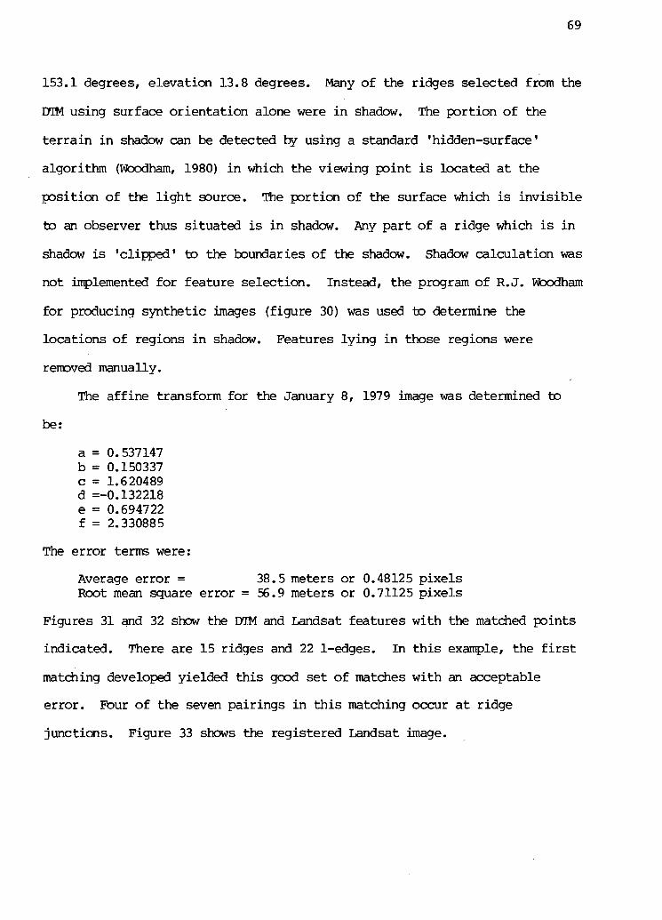
69

153.1 degrees, elevation 13.8 degrees. Many of the ridges selected from the

DTM using surface orientation alone were i n shadow. The portion of the

t e r r a i n i n shadow can be detected by using a standard 'hidden-surface'

algorithm (Woodham, 1980) i n which the viewing point i s located at the

position of the l i g h t source. The portion of the surface which i s i n v i s i b l e

to an observer thus situated i s i n shadow. Any part of a ridge which i s i n

shadow i s 'clipped' to the boundaries of the shadow. Shadow calculation was

not implemented for feature selection. Instead, the program of R.J. Woodham

for producing synthetic images (figure 30) was used to determine the

locations of regions i n shadow. Features l y i n g i n those regions were

removed manually.

The affine transform for the January 8, 1979 image was determined to

be:

a = 0.537147 b = 0.150337 c = 1.620489 d =-0.132218 e = 0.694722 f = 2.330885

The error terms were:

Average error = 38.5 meters or 0.48125 p i x e l s Root mean square error = 56.9 meters or 0.71125 p i x e l s

Figures 31 and 32 show the DTM and Landsat features with the matched points

indicated. There are 15 ridges and 22 l-edges. In t h i s example, the f i r s t

matching developed yielded t h i s good set of matches with an acceptable

error. Four of the seven pairings i n t h i s matching occur at ridge

junctions. Figure 33 shows the registered Landsat image.

Figure 30 Synthetic image f o r January 8t 1979. Sun's position i s azimuth 153.1 degrees, elevation 13.8 degrees. The white box o u t l i n e s the portion of the DTM used i n feature s e l e c t i o n . Photographed from the screen of the COMT7AL V i s i o n 1.

71

72

Figure 33 Registered Landsat image section for January 8, 1979. The white square outlines the 10 kilometer area' covered by the DTM. Pnotographed from the screen of the COMTAL Vision 1.

74

5. Discussion and Conclusions

5.1 Discussion

The results of the tests indicate that feature matching can be an

eff e c t i v e procedure for registering images. Registration errors for the

examples are we l l within accepted standards. The automatic re g i s t r a t i o n

procedure presented r e l i e s upon the existence of a detailed t e r r a i n model

for i t s use. Currently, such DTM's are not generally available. However,

i n Canada, the Department of Energy, Mines and Resources i s committed to

production of such DTM's for most of Canada. I t has been shown (Woodham,

1980) that r e g i s t r a t i o n of an image to a d i g i t a l t e r r a i n model i s help f u l i n

determining shading effects which af f e c t image analysis. Benefits such as

t h i s can sometimes j u s t i f y manual generation of a DTM for a p a r t i c u l a r study

area.

Insofar as the method i s based upon determining t e r r a i n features which

w i l l appear d i s t i n c t l y i n an image, the method i s r e s t r i c t e d to application

i n areas of mountainous t e r r a i n . There i s l i t t l e p o s s i b i l i t y that the

method as i t stands would be useful i n registering images of p r a i r i e land.

The benefits of registering an image to a DTM i n such a situ a t i o n are

minimal also. Nevertheless, the p r i n c i p l e of using known illumination

conditions and a scene model can find a p p l i c a b i l i t y elsewhere. The features

selected can be water-land boundaries, roads and other d i s t i n c t i v e scene

elements. The application to DTM's and Landsat images i s p a r t i c u l a r l y

appealing since the imaging geometry i s simple. There i s no need to solve

hidden surface problems. Funt (1980) has proposed using synthetic images i n

75

interpreting indoor scenes. Features extracted from any scene model

containing information on surface orientation and position can be used with

the method presented.

The representation of curves by generalization s i m p l i f i e s the process

of analysing the relations between curves. By matching portions of curves

to each other i n varying positions, d i s t i n c t i v e matchings are determined.

Although the notion of representing a curve by i t s band has existed for some

time, i t s use i n curve matching i s new i n t h i s application. By permitting

looser matching between curves and segments of curves, the band

representation f a c i l i t a t e s curve matching.

Determining l o c a l support for a match appears to disambiguate f a l s e

matches readily. In images of mountainous t e r r a i n , i t i s u n l i k e l y that

l o c a l support w i l l be i n s u f f i c i e n t for detecting correct matches. However,

i n scenes of urban landscapes, or i n i n d u s t r i a l applications, r e g u l a r i t y i s

i n t r i n s i c . Local support w i l l be very necessary i n distinguishing f a l s e and

true matches. In addition, these situations w i l l require more careful

selection of d i s t i n c t subsets of matching features. The representations for

curves advanced i n t h i s thesis i s advantageous for such feature selection.

D i f f i c u l t i e s with the method w i l l occur i n areas of low r e l i e f or

strongly regular t e r r a i n , what geomorphologists c a l l "strongly controlled"

t e r r a i n . Clouds, depending upon the sun's position, can be problematic.

The boundaries of shadows of clouds w i l l appear i n images as strong

brightness di s c o n t u i t i e s and w i l l not be discriminated from the images of

ridges. Clouds themselves w i l l generate brightness d i s c o n t i n u i t i e s . The

method may prove i t s e l f robust enough to meet t h i s challenge.

76

5.2 Further Work

The handling of curve matching where both curves are structured was

eliminated i n t h i s implementation of the regi s t r a t i o n method. By

subdividing l-edges into simple segments, some of the power of the

representation i s l o s t . The junctions at which the 1-edge segments meet are

then unavailable. However, the implementation i s s i m p l i f i e d . By including

a f a c i l i t y for manipulating and assessing structured-to-structured feature

matching a s i g n i f i c a n t improvement oould be made. Davis (1979) has

developed one such method.

The control of matching development i s very simple. All

translation-consistent t r i p l e s are examined for self-consistency. I f a

matching i s self-consistent with respect to i t s derived transformation, the

transform i s used to predict the location of image features i n the DTM. The

re s u l t of t h i s test of the transform i s binary: either accept or f a i l . When

a set of predicted 1-edge to ridge overlaps i s generated, the s t r u c t u r a l

relations between the overlapping l-edges and ridges could be used to guide

further adjustment of the parent matching. This upward flow of information

i s very important i n image analysis i n general.

5.3 Conclusions

This work demonstrates the effectiveness of matching features derived

from d i g i t a l t e r r a i n models with image features for solving the r e g i s t r a t i o n

problem. I t i s hoped that the techniques presented here and the p r i n c i p l e s

underlying them can find application elsewhere.

77

Bibliography

Agin, G.J., "Computer Vision Systems for I n d u s t r i a l Inspection and Assembly", Computer 13, 5(May, 1980), 11-20.

Aho, A.V., Hopcroft, J.E. and J.D. Ullman,The Design and Analysis of Computer Algorithms, Addison-Wesley, Reading, Ma., 1974.

Ambler, A.P. and R.S. Popplestone, "Inferring the positions of bodies from specified s p a t i a l relationships", A r t i f i c i a l Intelligence, 6, 2 (1795), 157-174.

Bajcsy, R. and P. Chance, "Picture recognition applications i n biochemistry", Technical Report, University of Pennsylvania, Moore

'• School of E l e c t r i c a l Engineering, (May, 1975).

Bajcsy, R., and M. Tavakoli, "Computer recognition of roads from s a t e l l i t e pictures", International Joint Conference for Pattern Recognition, (1976).

Ballard, D.H., CM. Brown and J.A. Feldman, "An Approach to Knowledge-Directed Image Analysis", International J o i n t Conference on A r t i f i c i a l Intelligence, (1979).

Ballard, D.H. " S t r i p Trees: A Hierarchical Representation for Map Features", Proceedings of IEEE Computer Society Conference on Pattern Recognition and Image Processing, Chicago, I l l i n o i s , August 1979, 278-285.

Barnea, D.T. and H. Silverman,"A Class of Algorithms for Fast D i g i t a l Image Registration", IEEE Transactions on Computers, C-21, 179, (1972).

Barrow, H.G. and R.M. B u r s t a l l , "Subgraph Isomorphism, Matching Relational Structures and Maximal Cliques", Information Processing Letters, 4, 4, (Jan. 1976), 83-84.

Barrow, H.G. and R.S. Popplestone, "Relational descriptions i n picture processing", i n Machine Intelligence 6, Meltzer, B., Michie, D. (Eds.), 377-396.

Barrow, H.G., Tenenbaum, J.M., Bolles, R.C. and H.C. Wolf, "Parametric Correspondence and Chamfer Matching: Two New Techniques for Image Matching", Technical Note 153, SRI International, Menlo Park, C a l i f o r n i a .

Bernstein, R. " D i g i t a l Image Processing of Earth Observation Sensor Data", IBM Journal of Research and Development, (Jan. 1976), 40-57.

Bolles, R.C, "Robust feature matching through maximal cliques", Proceedings of Society of Photo-optical Instrumentation Engineers, 182 Imaging Applications for Automated In d u s t r i a l Inspection and Assembly, (1979), 140-149.

78

Bolles, R.C. et a l . , "Automatic Determination of Image-to-Database Correspondences", International J o i n t Conference on A r t i f i c i a l Intelligence, (1979).

Davis, L.S. "Shape Matching Using Relaxation Techniques". IEEE Transactions on Pattern Analysis and Machine Intelligence, 1,1 (Jan. 1979), 60-72.

Davis, L.S. "A Survey of Edge Detection Techniques", Computer Graphics and Image Processing 14, 3 (1975), 248-270.

Davis, W.A. and S.K. Kenue, "On the Detection of Changes i n D i g i t a l Images", Computer Science Technical Report, University of Alberta, Edmonton, (Sept. 1977).

Fi s c h l e r , M.A. and R.A. Elschlager, "The Representation and Matching of P i c t o r i a l Structures", IEEE Transactions on Computers, C-22, 1, (Jan. 1973), 67-92.

Fowler, R.J. and J . J . L i t t l e , "Automatic Extraction of Irregular Network D i g i t a l Terrain Models", Proceedings of SIGGRAPH-79, Chicago, I l l i n o i s , (Aug. 1979), 199-207.

Funt, B.V. "Towards Synthetic Images i n Scene Analysis", Proceedings of the CSCSI/SCEIO Conference, V i c t o r i a , B.C., (1980), 158-165.

Horn, B.K.P., "The Position of the Sun", MIT A l Lab Working Paper 162.

Horn, B.K.P. and B.L. Bachman, "Using Synthetic Images to Register Real Images with Surface Models", Comm. ACM 21, 11 (Nov. 1978), 914-924.

Horn, B.K.P. and R.J. Woodham, "Landsat MSS Coordinate Transformations", Proceedings of the F i f t h Annual Symposium on Machine Processing of Remotely Sensed Data, Purdue University, 1979.

Hsieh, Y.Y. and K.S. Fu, "A Method for Automatic IC Chip Alignment and Wire Bonding", Proceedings of the IEEE Computer Society Conference on Pattern Recognition and Image Processing, Chicago, I l l i n o i s , (August 1979), 101-108.

Iannino, A. and S. Shapiro, "An Iterat i v e Generalization of the Sobel Edge Detection Operator", Proceedings of the IEEE Computer Society Conference on Pattern Recognition and Image Processing, Chicago, I l l i n o i s , (August, 1979), 130-137.

I t a i , A., Rodeh, M. and S.L. Tanimoto, "Some matching problems for b i p a r t i t e graphs", Journal of the Association for Computing Machinery 25, 4 (Oct. 1978), 517-525.

J o l l i f e , B. and B.W. Pollack, "UBC PASCAL, PASCAL/CJBC Programmer's Guide",Computer Center, University of B r i t i s h Columbia, (Sept. 1979).

Kaneko, T., "Evaluation of LANDSAT Image Registration Accuracy", Photogrammetric Engineering and Remote Sensing XLIII, 1976, 1285-1299.

79

Myers, W., "Industry Begins to Use V i s u a l Pattern Recognition", Computer 13, 5 (May, 1980), 21-31.

Nevatia, R. and K.R. Babu, "Linear Feature Extraction and Description", International J o i n t Conference on A r t i f i c i a l Intelligence, (August,1979).

P a v l i d i s , T.,Structural Pattern Recognition, Springer-Verlag, New York, 1977.

Peucker, T.K. and D.H. Douglas, "Detection of surface-specific points by l o c a l p a r a l l e l processig of discrete t e r r a i n elevation data", Computer Graphic and Image Processing 4, (1975), 375-387.

Peucker, T.K., R.J. Fowler, J . J . L i t t l e , and D.M. Mark, "The Triangulated Irregular Network", Proc. of the D i g i t a l Terrain Models Symposium, May 9-11, 1978.

Ramer, U. "An i t e r a t i v e procedure for the polygonal approximation of planar curves". Computer Graphics and Image Processing 1,3 (1972).

Sutherland, I.E., Sproull, R.F. and R.A. Schumaker, "A Characterization of Ten Hidden-Surface Algorithms", Computing Surveys 6, 1 (March 1974), 1-55.

Tanimoto, S.L. "Analysis of biomedical images using maximal matching", Proceedings of 1976 IEEE Conference on Decision and Control Adaptive Processes, Clearwater Beach, F l a . , (Dec. 1976), 171-176.

Toriwaki, J . and T. Fukumaru, "Extraction of Structural Information from Grey Pictures", Computer Graphics and Image Processing 7, (1978), 30-51.

Wilcox, B. and C. Hafner,"LISP/MTS User's Guide", Department of Computer Science, University of B r i t i s h Columbia, (July, 1976).

Woodham, R.J. "Using D i g i t a l Terrain Data to Model Image Formation i n Remote Sensing", Proc. Soc. Photo-Optical Instrumentation Engineers, Vol. 238, Bellingham, Wa., (July, 1980).