UPTEC X 11 008

Examensarbete 30 hpMars 2011

Automatic detection of fluorescent spots in microscopy images

Anel Mahmutovic

Molecular Biotechnology Programme

Uppsala University School of Engineering

UPTEC X 11 008 Date of issue 2011-02

Author

Anel Mahmutovic

Title (English)

Automatic detection of fluorescent spots in microscopy images

Title (Swedish)

Abstract A GUI(Graphical User Interface)-based spot detection software was designed and implemented in Matlab, having both manual and automated capabilities. It supports 7 spot detection methods, image cropping, colony segmentation, deletion/addition of spots and more. The spot detection methods have been evaluated using FROC(Free-response Reciever Operating Characteristics) methodology and the software has been used in studying real world problems. Some of these problems are the investigation of the expression pattern of LacI molecules and the creation of cell lineage trees.

Keywords Spot, Image, Matlab, Filtering, Morphology, FROC, Gaussian, Fluorescence, LacI

Supervisors

Gustaf Ullman (ICM), Johan Elf (ICM)

Scientific reviewer

Ewert Bengtsson (CBA)

Project name

Sponsors

Language

English

Security

ISSN 1401-2138

Classification

Supplementary bibliographical information Pages

35

Biology Education Centre Biomedical Center Husargatan 3 Uppsala

Box 592 S-75124 Uppsala Tel +46 (0)18 4710000 Fax +46 (0)18 471 4687

Automatic detection of fluorescent spots

in microscopy images

Anel Mahmutovic

Sammanfattning

Fluorescensmikroskopi tillåter forskare att studera enskilda molekylers dynamik. En sådan,

statisktiskt signifikant, studie kräver enorma datamängder. Analysen av datan är följaktligen

flaskhalsen då man går från experiment till att utröna den underliggande biologin. Ett av

analysstegen är oftast prickdetektion i mikroskopibilder av biologiska system, där varje

fluorescent prick motsvarar en molekyl. Sättet på vilket prickarna har detekterats hittills har

varit manuellt, dvs peka och klicka på varje prick i varje bild. Av diverse olika skäl, men

främst för att undvika subjektiviteten som följer den manuella metodologin, har en

prickdetektions-mjukvara skapats. Mjukvaran kallad BlobPalette3, programmerades i Matlab

vilket är ett programmeringsspråk väl utrustat för att tackla komplexa bildanalysproblem.

BlobPalette3 är ett GUI-baserat program innehållande 7 av de mest välanvända

prickdetektionsmetoderna enligt vetenskapliga artiklar. Vidare har BlobPalette3 möjlighet

att segmentera cell-kolonier, lägga till prickar, ta bort prickar, beskära bilder m.m.

BlobPalette3 detekterar prickar antingen semi-automatiskt eller automatiskt. Det semi-

automatiska tillvägagångssättet är att ladda in ett bildset i programmet, välja metod, ställa in

parametrar och detektera prickar. Det automatiska tillvägagångssättet åstadkoms genom att

integrera BlobPalette3 med det java-baserade programmet μManager, vilket är ett program

för kontroll av automatiserade mikroskop. Metoderna evaluerades med FROC-metoden där

det visade sig att prickdetektionsmetoden baserad på den så kallade Wavelet-Transformen

var bäst (relativt vår typ av bilder). BlobPalette3 har exempelvis börjat användas till att skapa

cell-släktträd innehållande prickinformation samt till att studera interaktionen mellan

transkriptionsfaktorn LacI och DNA. Den kontinuerliga utvecklingen av prickdetektions-

algoritmer tillsammans med den evolution BlobPalette3 genomgår, kommer att säkerställa

mjukvarans roll i utforskandet av livets hemligheter.

Examensarbete 30hp

Civilingenjörsprogrammet i Molekylär Bioteknik

Uppsala universitet februari 2011

1

Contents Page

1. Introduction 2

1.1 The lac operon 2

1.2 Image Analysis Fundamentals 4

1.2.1 Spatial Filtering 4

1.2.2 Morphological Image Processing 6

2. Methods 10

2.1 Top-Hat-Filter 10

2.2 Grayscale Opening Top Hat Filter 11

2.3 SWD (Stable Wave Detector) 13

2.4 FDA (Fishers Discriminant Analysis) 13

2.5 IUWT (Isotropic Undecimated Wavelet Transform) 16

2.6 RMP (Rotational Morphological Processing) 18

2.7 H-Dome transform 19

3. Evaluation 19

3.1 ROC (Reciever Operating Characteristics) 20

3.2 FROC (Free-Response ROC) 22

4. The software (BlobPalette3) 23

5. Results 25

6. Discussion 29

6.1 Dealing with the noise variability between images 29

6.2 The evaluation 30

7. Conclusion and Future Perspectives 31

8. Related sub-projects 31

9. References 34

2

1. Introduction

The introduction of Fluorescence Microscopy techniques makes it possible to answer many

of the previously unanswered questions in various branches of Biology. Two examples of

those questions are how transcription factors (TFs) coordinate gene expression at the level

of single cells[18] and how small regulatory RNAs are distributed in the cell at each time

during the cell cycle. A more specific problem, lying closely at heart of this thesis, is the

investigation of what happens with a transcription factor when it is bound to DNA during

replication. The Elf group at the department of Cell and Molecular Biology, University of

Uppsala, has taken a significant step toward answering that question using novel microscopy

technology and computational tools. By using the lac operon in the E.coli cell as a model

system, in which a fusion protein is expressed in low copy numbers, the need arises for the

detection of single molecules. An imaging setup meeting that need is the Single Molecule

Microscopy technique[18]. The single molecule microscope is a wide-field fluorescence

microscope with fine tuned parameters, applied on single cells. The cells themselves have

carefully designed genetic constructs such that single fusion proteins are made visible in

fluorescence images. The single molecule visibility poses restrictions on how the genetic

constructs can be made. The major factors that need to be taken into account are the

maturation time for the fusion protein and the copy number of that protein.

First, the maturation time for the fluorescent molecule should be short. The maturation time

is the time it takes between the translation of the fluorescent protein and its ability to be

able to emit light upon excitation. A fluorescent fusion protein with short maturation time

ensures its binding site being occupied by a protein which is detectable.

Second, the copy number should be small. Having a large number of fast diffusing

fluorescently labeled proteins would produce a smear of signals, thus diminishing single

molecule detectability. The fast diffusing molecules still exist in a system having a low copy

number, but the contrast between a bound fusion protein and freely diffusing proteins is

sufficiently large to ensure single molecules being detectable.

The detected signals, i.e. immobilized fluorescing molecules, will appear as diffuse,

diffraction limited spots in images. To reveal the underlying biological processes from image

data one needs to quantitatively analyze the spots. Due to the noise present in biological

systems, large data sets are required in order to draw valid conclusions. Therefore, the aim

of this work was to construct an user friendly, robust, and accurate software capable of

detecting spots automatically and in real time during the image acquisition process.

3

1.1 The lac operon

The transcription of the lac operon(Fig.1) is induced when the availability of glucose is scarce

in order to metabolize the disaccharide allolactose, a metabolite of lactose[19]. Under

conditions where Glucose is available, the lac operon is repressed by the tight binding of the

transcription factor LacI to the operator site O. When the availability of glucose is running

low the intracellular cAMP (cyclic Adenosine Monophosphate) levels increase. The enhancer

CAP (Catabolite Activator Protein) proteins subsequently bind to cAMP molecules which

induces an allosteric effect in the CAPs leading to an increased affinity for their binding site.

This leads to an increased transcription rate of the lac operon. Furthermore, the binding of

allolactose to LacI results in the release of LacI from its binding site, causing a further

increase in transcription rate. The genes transcribed, that is to say lacZ, lacY and lacA, of

which only lacZ and lacY are necessary for the metabolizing function of the lac operon

system, encode the proteins β-Galactosidase, β-Galactoside Permease and β-Galactoside

transacetylase, respectively. The function of β-Galactosidase is to cleave the allolactose

producing one Glucose and one Galactose. β-Galactoside Permease is a membrane protein

that pumps lactose into the cell and β-Galactoside transacetylase transfers an acetyl group

from acetyl-CoA to galactosides.

Fig.1 Figure depicts the genetic organization of two E.Coli strains, wt cells and SX701 cells.

For the wt cells we see the lacI gene, the CAP binding site, the promoter site P, the operator

site O, the lacZ gene, the lacY gene and the lacA gene. The genetic organization in the SX701

strain is the same except for lacY being substituted for tsr-Venus.

To answer the question of what happens with a transcription factor (LacI) when bound to

DNA during replication we utilized the SX701 strain. In this strain we have a fusion protein,

tsr-Venus, substituted for lacY. The fusion is between a fast maturing fluorescent protein

Venus (an YFP variant) and a membrane targeting peptide[1] tsr. The membrane targeting

peptide reduces the diffusion rate of the fluorescent molecule thus preventing signal spread

4

in the cytoplasm which leads to an increased spot contrast. Given automated spot detection

and segmentation solutions, we can quantitatively determine the gene expression at a

specific time during a cell’s life cycle and thus answer the posed question.

1.2 Image analysis fundamentals

A digital image can mathematically be defined as:

where (i,j) is the pixel coordinate of the image and I is the intensity levels of the image. For

example the notion of a 8-bit grayscale image means that the number of intensity levels that

can be represented in the image is equal to 28=256 where a 0 equals to the color black, 255

is white and everything in between is different shades of gray. The plane {(i,j); i=1,2,…,M ,

j=1,2,..,N} is called the spatial plane of the image. An image containing the pixel values 1 or 0

is called a binary image.

When developing algorithms, a useful representation of a digital image when developing

algorithms is in matrix form (eq.2).

. . .

. . . (2)

. .

. . .

If I is given in matrix form, we have the power of directly manipulating the intensity values of

the image.

1.2.1 Spatial Filtering

In spatial filtering, one is referring to intensity value manipulations in the spatial plane. A

spatial filter, or mask, is a sub-image or sub-window with a predefined size and operation

(Fig.2).

1/9 1/9 1/9

1/9 1/9 1/9

5

1/9 1/9 1/9

Fig.2 An average filter of size 3x3 pixels.

We denote a filter of size mxn with w(s,t) such that w(0,0) is the value of the center

coordinate of the mask. Also, for our purposes, we will always work with odd sized filters

meaning that m=2a+1, n=2b+1 where a and b are positive integers. Then the process of

spatial filtering an image can mathematically be stated as:

where g(i,j) is the intensity value at coordinate (i,j) of the filtered image f and w is the filter.

The mechanics of (2) can be described as a process whereby w(0,0) visits every pixel (i,j) and

for each (i,j) computes the sum of products of w(i,j) with its corresponding f(i,j) and finally

maps the result of the computation to g(i,j). The border pixels are taken care of by

symmetric mirroring. The convolution of an image with a mask w is given by (3). Therefore,

spatial filtering an image with a mask w is the same as convolving an image with mask w. The

reader might also encounter the term correlation eq.(4). Having an isotropic filter, like the

average filter in Fig.2, the results of convolution and correlation are the same.

Noise in images arise due to the electronics of the hardware (Gaussian noise) and the

stochastics of photon emission from fluorophores (Poisson noise)[20]. Another source of

Poisson noise is low photon count[20]. The average filter, and other so called smoothing

filters, are usually used as a pre-processing step in order to reduce that noise. One filter that

is especially valuable for that purpose in our case is the Gaussian filter (Fig.3). Given that the

spots we are trying to detect are Gaussian, the Gaussian filter enhances these spots apart

from reducing the noise. This is because the spots, to a high degree of accuracy, can be

modeled using a Gaussian function. Therefore, we always use this filter as a pre-processing

step.

.0751 .1238 .0751

.1238 .2042 .1238

6

Fig.3 An example of a Gaussian filter with size 3x3 pixels and standard deviation 1 pixel.

1.2.2 Morphological Image Processing

Morphological image processing [21] is an extremely powerful tool in image processing

applications. It can for example be used for bridging gaps that exists in letters, reducing the

noise in fingerprint images, extract boundaries, filling holes, detect spots etc. It is based on

the mathematics of set theory where a set/subimage/structuring element is defined.

Subsequently, certain operations with that structuring element are applied on an image. For

our purposes, we shall mainly be interested in three specific operations called morphological

opening, closing and grayscale reconstruction by erosion. The morphological opening and

closing are described below. First, let us denote our structuring element by B which is a

member of 2-dimensional set of integers. Assume we perform the morphological operations

on a binary image A. The reflection (Fig.4), B’, and translation (Fig.5), (B)z ,of the structuring

element B are defined in equation (5) and (6), respectively.

B’ = (5)

(B)Z = (6)

Fig.4 An illustration of a structuring element B and its reflection B’.

.0751 .1238 .0751

7

Fig.5 An illustration of a structuring element B (left) and its translation (B)Z (right).

The erosion and dilation of an image A by structuring element B are given in equation 7 and

8, respectively.

A-B = (7)

A+B = (8)

What equation (7) tells us is that the erosion of image A is obtained by translating the

structuring element B such that B is contained in A. The region mapped out by A with

respect to its “center of mass” is then the eroded image. We will only be dealing with

structural elements that are either disk shaped or quadratic, therefore the center of mass is

always at the center of B and B’=B. This process is illustrated in Fig.6.

Equation 8 tells us that a dilated image A+B is produced by the reflection of the structural

element B around its center of mass followed by the translation such that B is always partly

contained in A. Note that due to symmetry, for our structural elements B’ = B. The process of

dilating an image A with a structural element B is illustrated in Fig.7.

8

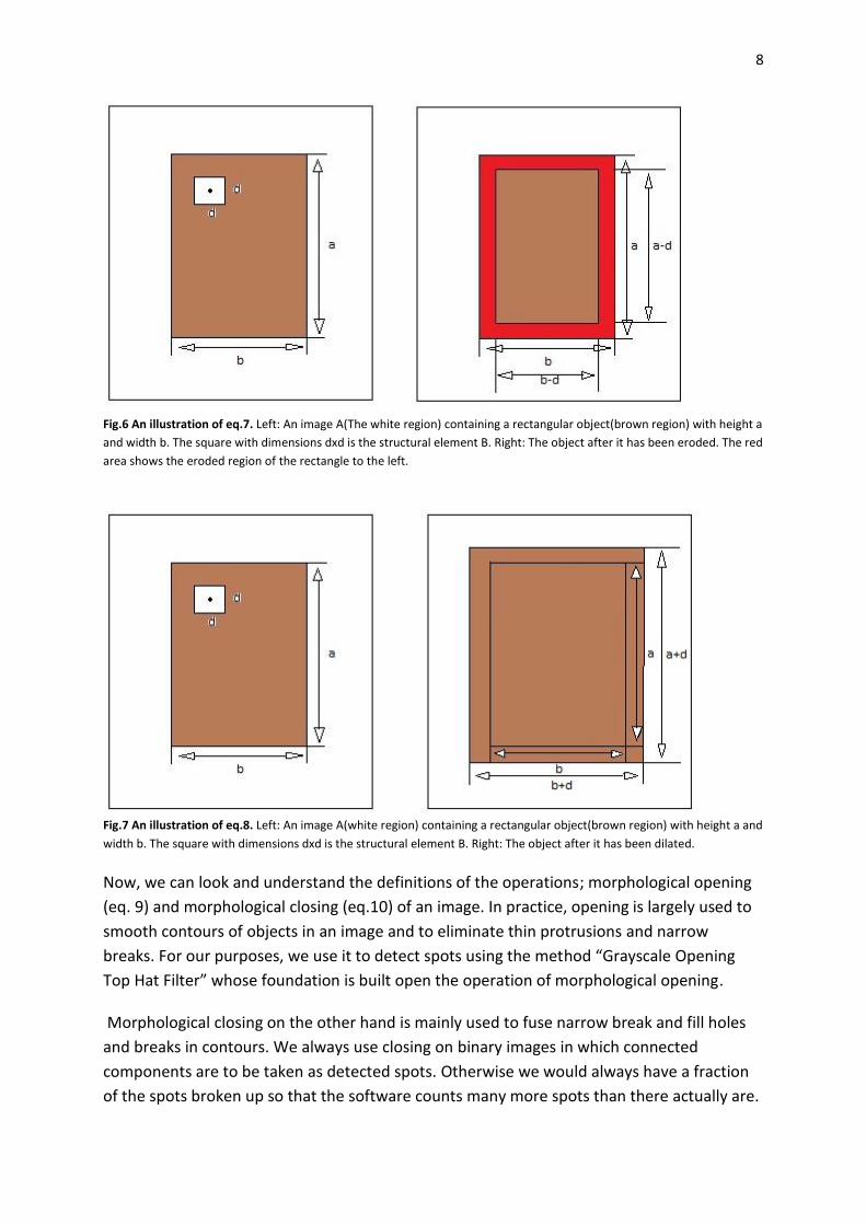
Fig.6 An illustration of eq.7. Left: An image A(The white region) containing a rectangular object(brown region) with height a

and width b. The square with dimensions dxd is the structural element B. Right: The object after it has been eroded. The red

area shows the eroded region of the rectangle to the left.

Fig.7 An illustration of eq.8. Left: An image A(white region) containing a rectangular object(brown region) with height a and

width b. The square with dimensions dxd is the structural element B. Right: The object after it has been dilated.

Now, we can look and understand the definitions of the operations; morphological opening

(eq. 9) and morphological closing (eq.10) of an image. In practice, opening is largely used to

smooth contours of objects in an image and to eliminate thin protrusions and narrow

breaks. For our purposes, we use it to detect spots using the method “Grayscale Opening

Top Hat Filter” whose foundation is built open the operation of morphological opening.

Morphological closing on the other hand is mainly used to fuse narrow break and fill holes

and breaks in contours. We always use closing on binary images in which connected

components are to be taken as detected spots. Otherwise we would always have a fraction

of the spots broken up so that the software counts many more spots than there actually are.

9

(9)

(10)

As is evident from equation (9), the opening of an image A by structural element B is the

erosion of A followed by dilation of (A-B). This particular sequence of operations is so

common that a name for it was introduced, morphological opening. Understanding why the

sequence is common follows from the following simple thought experiment. If we choose a

structural element B such that B is larger than the object/objects we would like to eliminate,

then eroding the image will not only eliminate the object of interest but also diminish other

objects. Then by dilating the image we force the diminished objects back towards their

original size.

The same is true for the closing operation (a dilation followed by erosion). Imagine, for

example, scanning a text. Now looking at the text you notice gaps in the letters. The fix for

this would be to first dilate the image containing the text. Since the letters now are too fat it

is preferable to erode the image in the next step.

The back and forth hopping between the opening and closing operators are far from perfect

when comparing the result with the original image. However there exist a powerful concept

known as morphological reconstruction with which hopping is unnecessary. We use this

concept to define the H-Dome transform, section 2.7. Applying morphological reconstruction

by dilation on an image that has been eroded, will result in exactly the original image minus

the objects that were eliminated by the erosion.

The concept of reconstruction by dilation and reconstruction by erosion is built upon

geodesic dilation (eq.11) and geodesic erosion (eq.12), respectively. In these equations we

have a marker image F, a structural element B and a mask image A. So, the meaning of

equation 11 for example, is that we dilate a marker image F with a structural element B

followed by a logical AND operation with mask image A. Then it follows, that if we apply

equation 11 successively using an eroded image as the marker and the original image as the

mask, we will end up with the original image minus the eroded objects given that the width

of B is smaller than the distance between the eroded objects and non-eroded objects. This is

exactly what the definition of morphological reconstruction by dilation (eq.13) means.

Stability in the recursive equation 13 is reached when DA(k)(F)=DA

(k+1)(F). Morphological

reconstruction by erosion is stated in eq. 14.

(11)

(12)

(13)

10

(14)

As noted above, we have been dealing with definitions of morphological operations on

binary images. Of course, the operations are also applicable to grayscale images where each

pixel is a member of Z3. In other words, each pixel has a coordinate (x,y) and an intensity

value A(x,y), all real integers in our case. Structuring elements in gray-scale morphology

come in two flavors, nonflat and flat. Our interest lies only in the flat structural elements

containing only 1s or 0s. Now, erosion of a gray-scale image with a flat structural element B

is defined in equation (11). The interpretation is that the “center of mass” of B visits every

pixel (x,y) in image A and for each (x,y) chooses the minimum value of A encompassed by B.

The process of dilating a gray-scale image A is similar to dilating it only that the maximum

pixel value is chosen (eq.12). The reason for the minus signs in equation (12) is because B

has to be reflected around its center of mass, B’ = B(-x,-y).

= (14)

(15)

The opening and the closing of a gray-scale image are given in equation (9) and (10),

respectively. The geodesic dilation, geodesic erosion, morphological reconstruction by

dilation and morphological reconstruction by erosion for grayscale images are as defined in

equation 11-14 except that we use the pointwise minimum operator and the pointwise

maximum operator instead of the logical AND for geodesic dilation and geodesic erosion,

respectively.

2 Methods

The methods implemented in the software fall into one of two categories. They are either

supervised or unsupervised, FDA (Fisher’s discriminant analysis) being the one method

falling into the supervised category. The logical flow by which all the methods (excluding FDA

from step 2 and 3) operate can be summarized in the following steps:

1. Reduction of the noise in images. This is done by spatial filtering the images with a

Gaussian kernel. Some of the methods, like the Top-Hat-Filter and the wavelet

transform, have intrinsic noise reduction capabilities. For these methods, the

freedom of choice exist for exists for choosing a pre-filtering step.

2. Spot enhancement. The way by which the methods enhance spots is what separates

one method from the other. The result from this step is a gray-scale image which can

be thought of as a probability map. The brighter the pixel the higher the probability

of it being a spot.

3. Binarization by the application of an intensity threshold. This step produces a binary

image IB(x,y) . The connected pixels of the binary image are clustered, each

11

cluster being a spot. The coordinates of the spots are taken as the centroids of the

clusters.

2.1 Top-Hat-Filter

The method of extracting spots using the top hat filter as described by [22] utilize the

intensity and size information of the spots. The idea is to define two circular regions DTop and

DBrim which are related to the maximum expected spot radius and the shortest expected

distance between spots, respectively (eq. 17,eq. 18,Fig.8). The idea is to let the regions DTop

and DBrim visit every pixel (i,j) in image I and for each (i,j) compute the average intensities ITop

and IBrim after which we apply (eq.19). The connected components are finally taken to be the

detected spots. The idea in computing the average intensities is to reduce the noise. The

meaning of the parameter H is the minimum rise of a pixel region above its background for

which we would consider that region a spot. So in summary, this method has three

parameters (H,DBrim,DTop). The method works well for images with relatively high signal-to-

noise (SNR) ratios, above 3. As for our images, the method is not suitable due to the low

SNR. Nevertheless, the method is computationally inexpensive so that it may be the method

of choice in the future due to the constant improvement of the image acquisition hardware.

DTop RTop2 (17)

DBrim RTop2 2 2 RBrim

2} (18)

CB(i,j) (19)

Fig.8 The red region corresponds to DTop while the blue region corresponds to DBrim.

2.2 Grayscale Opening Top Hat Filter

Grayscale Opening Top Hat Filter[3] makes use of the morphological operation known as

opening. In the area of spot detection, the idea is to first choose the radius of the disk-

shaped structuring element A such that rA > the radius of the largest expected spot. Then

12

grayscale opening is performed according to equation (x) on image J whose output is the

image JA. By doing the opening operation we have effectively removed all spherical objects

in the image whose size is smaller than that of the structuring element. Therefore, by taking

K = J-JA we remove in the image all non-spot objects. Of course, the image K will be

contaminated, so that the last step of this method is to threshold the image according

eq.(20).

CB(i,j) = (20)

The connected components are finally counted and taken as the spots. The algorithm is

depicted in fig.9. A common application of this method is actually removal of non-uniform

illumination on images that are to be segmented. The idea is as above, you take a structuring

element larger than all the objects and perform grayscale opening. This leaves you with only

the non-uniform background of the resulting image. Subtracting that image from the original

leaves you with objects without the non-uniform background.

13

Fig.9 A scheme depicting the algorithm of the Grayscale Opening Top Hat Filter. The image was generated by

randomly extracting 10 spots from real images and by randomly distributing them throughout the image.

1. The image is opened with a disk-shaped structure element with radius 10 pixels.

2. The image from 1 is subtracted from the original image.

3. The image is thresholded, resulting in a binary image.

4. The centroids of the connected components in the binary image are taken as the coordinates of the

spots.

2.3 SWD (Stable Wave Detector)

The idea behind the SWD (Stable Wave Detector) [23] is easily grasped if one starts with

considering a 1-D data array of length N and the signal of interest having a length of T/2.

From this data array we form a new one consisting of n overlapping frames where the

frames overlap more than T/2. For each frame i, we then compute the Fourier coefficients ai

and bi according to equation (21) and equation (22), respectively.

Finally, we say that a spot has been detected if (ai < |bi|) and the signal is surrounded by

bi<0 and bi>0 from left to right, respectively. The extension to 2-D is the application of

equation (21) and (22) first row by row followed by column by column. The intersection

between the positions are then chosen as the location of the individual detected blobs.

2.4 Fishers Discriminant Analysis (FDA)

The method of FDA[1,2,4,5] lies in the domain known as Pattern Recognition Methods and is

perhaps best introduced by describing an experiment Ronald Aylmer Fisher performed 1936.

The idea was to have a “machine” to distinguish between the two species of flowers Iris

14

setosa and Iris versicolor based on measurements (actually, yet another species Iris virginica

was used in Fishers article, but we omit it since our purpose is to introduce the reader to the

general concepts and terminology of discriminant analysis.). The measurements were the

petal length and width of each flower. By plotting the petal length and petal width against

each other he noticed two clearly discernable clusters of 2D points, each point representing

a flower (Fig.10) and each cluster representing a species. Given a mathematical expression

that can find a line that best separates the clusters from each other, the problem of

automatically detecting which flower belong to which species would be solved. Because

then, all you would have to do is measure the petal width and petal length of the flower and

check which side of the line the measurement fall on.

Fig.10 By measuring and plotting the petal width (x1) against petal length (x2) for flowers of the species Iris

setosa and Iris versicolor, R.A. Fisher saw two distinguishable clusters. Note that this is not the actual result Fisher got, the

figure merely illustrates the idea.

The measurements x1 and x2 are components of what we define as a feature vector x (eq.

23).

(23)

The two iris species are defined as classes, w1 and w2, such that if x fall on the left side of the

discriminating line, then x w1 if we define the left cluster in Fig.10 as w1. A discriminant

function di(x) is a function such that di(x)>dj(x) , i,j if x wi and i j. Clearly then, the

discriminating line or decision boundary is given by equation 24.

dij=

Given a decision boundary dij(x), we just check the sign and assign the feature to the proper

class. Of course, finding a decision boundary in the first place requires collecting training

15

data. In our example above, we would need to collect a substantial amount of I.Setosa and

I.Versicolor flowers, make the measurements and undertake a suitable approach to find

dij(x). The “suitable approach” that we shall be interested in is the FDA approach. First, we

define a discriminant function di(x) according to equation 25.

i| (25)

(26)

Ni is the number of features belonging to class wi. The mean vector of class i, μi, can be

thought of as a vector pointing to the center of mass of the cluster representing class i. The

vector, w, is found by finding the maximum of the ratio (Q(w)) given in equation 27. Clearly,

maximizing Q means that we try to find a w such that we get a maximum separation

between classes with respect to their mean vectors and at the same time a minimum intra

class variance (since is the covariance matrix of class i). In finding such a w and applying

it in equation 24, we actually perform a linear transformation, the result being a mapping

from higher dimensional space on one dimension. The solution of setting is given in

equation 28 where μi is the mean vector of class i.

(27)

-1 (28)

For our spot detection purposes, we defined two classes, one being spots and the other

being background. The training data consists of 5x5 image patches of spots and background

such that xT = (x1,x2,…,x25). The decision boundary will thus be a hyperplane in 25

dimensional space. The method has no parameters but it requires collecting training data

which can be really cumbersome, especially if one has to collect 5x5 image patches by hand.

Initially, we noticed the results being highly sensitive to the amount and quality of the

training data we collected. It was cumbersome to collect enough material because of the

unmanageable ratio between the amount of manual work per image patch versus the

amount of data needed. Therefore, we used the wavelet transform to collect the data in a

semi-automatic fashion where the threshold was set to a high value to ensure the quality of

the data (Fig.11).

FDA is widely used throughout the scientific community for example, in differentiating

between normal and adenocarcinoma tissue in an early stage[4], in automatic identification

of β-barrel membrane proteins[6], in quality control[7], etc. The success or failure for our

purposes depends largely on the assumption that the distribution of the samples are

multinormally distributed. This is the main prerequisite that FDA requires to ascertain

16

optimum performance. Even though the distributions may be normal, but there are

considerable overlap between the background and the spot distributions, the results will be

poor because FDA is a linear discriminator. Also, which features one choose and the quality

of the training data, are important considerations to make.

2.5 Isotropic Undecimated Wavelet Transform (IUWT)

The wavelet transform[1,8-10], which gave rise to the MRA (Multi Resolution Analysis)

approach in the field of signal processing, decompose a signal Aj0 at resolution j0 into signals

Aj where j=j0,j0+1,j0+2,…,j0+k. The signal in our case being an image, the wavelet transform

allow us to study it at different resolutions thus enabling us to detect features that might

otherwise go undected. It has been diligently used in image denoising and compression[11],

face recognition[12], astronomical image processing[9] and for many other purposes.

The scheme that we have adopted to detect the spots (à trous wavelet representation) using

the wavelet transform comes mainly from [1,8 & 13]. If we let j0=0 correspond to our input

image A0(x,y), then the approximation images A1,A2,…,Ak are generated by recursively

convolving the image A0 with the 1-D kernel [1/16 1/4 3/8 1/4 1/16] and inserting 2j-1 -1

zeros between every two taps. The insertion of the zeros in the filter/kernel is where the

name “à trous” came from, trous meaning hole. The next step is to compute the wavelet

planes according to equation 29 whereby we have decomposed our image in a set of

wavelet planes and the most coarse approximation image w1,w2,…,wk,Ak. With this set we

can easily reconstruct the original image without error by using eq. 30.

(29)

(30)

The adoption of the à trous representation gives rise to properties of the wavelet planes

which are crucial for the realization of detecting spots. First, the wavelet planes are

translation invariant, meaning that the detection of a spot does not depend on its position.

Second, the transform is not biased toward a particular direction in the input image, that is it

is isotropic. Third, local maxima in the wavelet plane will propagate down the resolution

levels due to significant discontinuities and not noise in the original image, given that the

image is corrupted by additive correlated Gaussian noise[14,15]. If the image is corrupted by

mainly poisson noise, then one applies the Anscombe Transform (eq. 31) which transforms

17

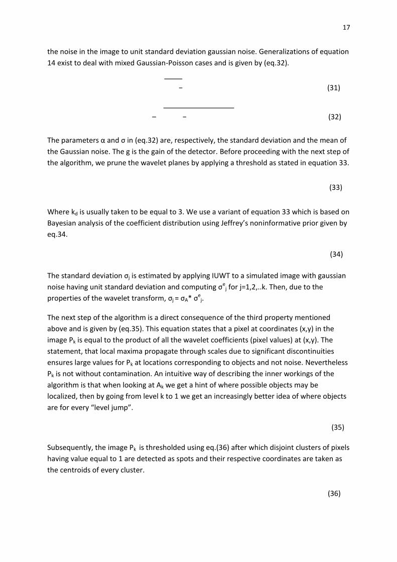
the noise in the image to unit standard deviation gaussian noise. Generalizations of equation

14 exist to deal with mixed Gaussian-Poisson cases and is given by (eq.32).

(31)

(32)

The parameters α and σ in (eq.32) are, respectively, the standard deviation and the mean of

the Gaussian noise. The g is the gain of the detector. Before proceeding with the next step of

the algorithm, we prune the wavelet planes by applying a threshold as stated in equation 33.

(33)

Where kd is usually taken to be equal to 3. We use a variant of equation 33 which is based on

Bayesian analysis of the coefficient distribution using Jeffrey’s noninformative prior given by

eq.34.

(34)

The standard deviation σj is estimated by applying IUWT to a simulated image with gaussian

noise having unit standard deviation and computing σej for j=1,2,..k. Then, due to the

properties of the wavelet transform, σj = σA* σej.

The next step of the algorithm is a direct consequence of the third property mentioned

above and is given by (eq.35). This equation states that a pixel at coordinates (x,y) in the

image Pk is equal to the product of all the wavelet coefficients (pixel values) at (x,y). The

statement, that local maxima propagate through scales due to significant discontinuities

ensures large values for Pk at locations corresponding to objects and not noise. Nevertheless

Pk is not without contamination. An intuitive way of describing the inner workings of the

algorithm is that when looking at Ak we get a hint of where possible objects may be

localized, then by going from level k to 1 we get an increasingly better idea of where objects

are for every “level jump”.

(35)

Subsequently, the image Pk is thresholded using eq.(36) after which disjoint clusters of pixels

having value equal to 1 are detected as spots and their respective coordinates are taken as

the centroids of every cluster.

(36)

18

The scheme where we go from original image to detected spots via Pk and a CBinary are shown

in Fig.12.

Fig.12 Top Left: Original Image. 1: Shows the wavelet multiscale product Pk. 2: Shows the result from applying eq.18 on

Pk. 3. The detected spots for the image.

2.6 RMP (Rotational Morphological Processing)

The method of RMP[16] utilize the grayscale top hat transformation using a linear structural

element of width 1 and length larger than the diameter of the spots one wishes to extract.

The idea is to apply the top hat transformation on N images, each image i being a rotated

(clockwise) version of the input image A0 as given in equation 37. The rotational part of this

method is there because spots are in general symmetric objects, thus an isotropic approach

to the detection of them is suitable (i.e. a linear structural element is not isotropic). The

19

whole purpose of the method is to increase the resolution with respect to a methods

capability to differentiate between spots that are very close.

-1 (37)

After applying the grayscale top hat transform on each image Ai->A’i, the images are rotated

anticlockwise and equation (38) is applied. This equation states that the pixel value at (x,y) in

image g is equal to the maximum intensity value at (x,y) for A’i. The effect of this equation in

combination with the application of a linear structural element on rotated versions of the

same image is the elimination of Gaussian objects and the retaining ,to a certain degree, of

the diffuse intensity bridge between 2 close spots. Therefore, by applying equation (39) and

subsequently thresholding the result one can detect closely lying spots.

(38)

(39)

2.7 H-Dome transform

The core of the H-Dome[1,16] transform is morphological reconstruction which it employs to

detect spots. Starting with the original image A0(x,y) as the mask, we apply equation 40 to

get the marker image F.

(40)

The constant h defines where image A0(x,y) is to be “sliced” relative to the maximum

intensity value A0(x,y). Then, we perform grayscale morphological reconstruction by dilation

given in equation 12. Note that we use the grayscale definition of dilation in the geodesic

dilation equation and that the logical AND operator is substituted for a pointwise minimum

operator. This gives us an image H, on which we apply equation 41 to get a binary image that

we subsequently use to detect spots. Note that this method does not have an intrinsic noise

reduction capability. Therefore, it is imperative that a nosie reduction step is included such

as spatial filtering with a Gaussian kernel. The effect of the Gaussian on H(x,y) would be

broadening of the objects, thus a parameter s is incorporated into the method which

transforms H(x,y)->Hs(x,y) to mitigate the broadening effect.

(41)

3 Evaluation

The evaluation of the spot detection methods was done using FROC[18] (Free Response

Operating Characteristics) methodology. ROC[18] (Receiver Operating Characteristics),

which has been diligently applied on evaluating medical diagnostic systems is the method

20

from which FROC was derived. Thus, ROC is explained in section 3.1 and FROC in section

3.2. Before proceeding, some basic terminology needs to be explained. Given a set of objects

each with a boolean state and the knowledge of which objects are true, then true positives

(TPs) are all the detected objects that coincide with the true objects. An analogous term used

for TPs in decision theory literature is sensitivity. True negatives (TNs) are all the objects

which have not been detected minus the true objects that have not been detected. The true

objects that have not been detected are false negatives (FNs). An analogous term for (TNs)

found in decision theory literature is specificity. Finally, false positives (FPs) are all the

detected objects that do not coincide with the true objects. The true positive fraction (TPF)

and the false positive fraction (FPF) are defined as and

, respectively.

3.1 ROC (Reciever Operating Characteristics)

Consider a system which has to determine whether an event is true or false. The system may

be a spot detector which is presented with multiple images (the objects in this case) and the

spot detector has to determine whether one or more spots are present (truth state of object) or

not (false state of object). The system in this case is then boolean, either it detects an image

having spots or it does not. The detector has a threshold; given a large threshold the detector

detects less spots than it would with a lower threshold, thus the probability for detecting an

image with spots is less. In other words, a large threshold means a small FP fraction but also a

small TP fraction. Conversely, by setting a lower threshold we would detect more TPs but

also more FPs.

This can be illustrated by plotting the intensity distribution of positive samples (spots) and

negative samples (background) with respect to the intensity values (Fig.13). By setting an

intensity threshold to a value x, the detector considers all samples as spots having an intensity

value larger than x. Therefore, setting the threshold at x=0.1, we get a (TP,FP)-pair where we

get many TPs and many FPs as is evident in the figure. If we now increment the threshold-

value over the whole intensity span by a step size of T and taking we can produce a

continuous curve by plotting TPF versus FPF. The continuous curve is denoted as a ROC

curve (Fig.14). The ROC curve is a complete description of our methods capability to detect

images with spots. We realize that given an ROC curve with the detector has a

50% chance of detecting the existence of spots (one distribution completely overlaps the

other). If , then the detector has a 100% chance of detecting the existence of

spots (no overlap between normal distributions if they are infinitely separated). Thus we

would take the area under the roc curve (AUC) as a measure of the methods capability to

detect the existence of an image with spots.

21

Fig.13 An illustration of the approximately binormal distribution of pixels corresponding to

spots and background. Note that the detector described in section 3.1 has nothing to do with

our spot detection methods. The fictive detector was introduced to simplify the minds transition

to the world of ROC curves.

Fig.14 An illustration of the appearance of 3 ROC curves. The probability of method green

detecting an image with spots is 1. The probability of method blue detecting spots an image

with spots is 0.67. The probability of method red detecting an image with spots is 0.50.

For our purposes we need a generalized ROC evaluation such that we take into account the

methods capabilities of detecting spots in images and not the images with spots. The

generalized ROC evaluation should also take the precision by which the spots are localized

into account.

22

3.2 FROC (Free-Response Receiver Operating Characteristics)

The first step towards the conception of the FROC methodology was the development of

LROC methodology (Localization ROC). Given an object with a location, zTRUE, and a state

which can be true or false; we define a true positive TP as a detected object which is true

and which is localized at zDetected if |zTRUE - zDetected| < otherwise it’s a FP. In our case we

have multiple objects (spots) that need to be detected to within an pixel (160 nm). The

extension of LROC is the detection of all the objects over all the images where TPs are scored

with respect to detection and location. Subsequently a curve (FROC curve) is produced by

plotting TPF versus the mean number of false positives per image (Fig.15). Note that the

FROC curve does not have an upper limit with respect to the number of FPs per image.

Therefore the AUC cannot be utilized to measure spot detection performance. Instead, we

will compare the TPF at a fix value of the mean number of false positives per image (<FPs>)

the implications of which are discussed in section 6.

Fig.15. A FROC curve where y-axis: True Positive Fraction and x-axis: mean number of False Positives.

23

4 The Software (BlobPalette3)

A definition list of the functions of BlobPalette3.

1. Load one or multiple images. The program has only been tested for .tiff images.

2. Saves multiple files associated with a spot detection session. The files are as follows:

# blobData.mat -> First column: x-coordinates, Second Column: y-coordinates, Third

Column: Frame number.

# cropData.mat -> A row vector which holds the x-position, the y-position, the width

of x and the height of y of a rectangle specifying how the original

image was cropped. Default = [90,85,217,280].

# imageStack.mat -> A 3D matrix of size [width_image x height_image x nr_images].

The matrix holds all images that were loaded.

# matsData.mat -> A vector of size nr_Frames holding the total number of detected

spots in each frame.

# savedcoords.mat -> A cell array of size nr_Frames. Each element holds a matrix

Containing the (x,y) coordinates of the detected spots.

3. This function is used if one wishes to synchronize BlobPalette3 with Micro-Manager,

a software package for control of automated microscopes. With this, one has the

capability of running an automated spot detection session in real time. The

operational flow is as follows: First, press (3) followed by Micro-Manager-1.3.

Second: Select MMTest2 in the plugins menu in Micro-Manager-1.3 (Fig.14). Third:

Define parameters for image acquisition session in Micro-Manager-1.3. Forth: Lean

back and enjoy.

24

Fig. 16 Micro-Manager, a software package for control of automated microscopes. Synchronization with BlobPalette3

requires selecting MMTest2 before image acquisition.

4. A listbox where you have the option of selecting between 7 methods.

5. A button which is activated when images are loaded. Pressing it will allow you to

define a crop rectangle, using the mouse, in the right image window whereby all

images are cropped.

6. Clears all detected spots in current frame showing the spots.

7. A checkbox, when pressed, lets you define a crop rectangle by specifying the (x,y)

position of its upper left corner, the width and the height.

8. Parameter area where parameters associated with the selected method shows up.

9. The button to press to detect blobs/spots.

10. Extract positive (spots) and negative (background) training data for FDA. The edit box

lets you specify how many negative samples you wish to collect. The software will

prompt you to save a number of files:

# Negative.mat -> a matrix with nr_negative_samples rows and 25 columns.

# Positive.mat -> a matrix with sum(matsData) rows and 25 columns.

25

# w.mat -> a column vector defining the linear transformation as explained in

section 2.4.

11. Lets you add blobs to images. Somewhat defeating the approach of non-subjectivity

towards spot detection. Use with caution.

12. Lets you delete blobs from images. Somewhat defeating the approach of non-

subjectivity towards spot detection. Use with caution.

13. Activation of colony segmentation using the wavelet transform when checked. Have

to specify the minimum colony area that you would expect.

14. Slider-control of which frame is currently shown (for frames containing detected

spots).

15. Slider-control of which frame is currently shown.

16. The currently shown frame with detected spots, image+frame number.

17. The currently shown frame, image+frame number.

Notes: The methods for spot detection are constantly evolving. The software has thus been

designed (at the code level) as a platform, onto which new methods can be added with

relative ease.

5 Results

The results from the evaluation of the methods using FROC methodology is presented in

Fig.16 and Table1. We used real image data of which 10 images were randomly selected.

The images were used as a golden standard, i.e. we assumed knowing the location of the

true spots in all 10 images. The SNR (Signal to Noise Ratio) for the images, which is an image

quality parameter, was estimated using positive and negative training data. It was calculated

by taking the difference between the mean intensity value for spots and the mean intensity

value for background patches, divided by the standard deviation of the spot intensities.

Fig.16 FROC curves for all methods except for FDA. Y-axis: True Positive Fraction

(TPF). X-axis: The mean number of false positives divided by the total nr of spots. The curves were

generated using 10 images, each image with a SNR 2.6. The total nr of true spots was 415.

26

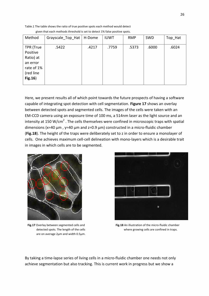
Table.1 The table shows the ratio of true positive spots each method would detect

given that each methods threshold is set to detect 1% false positive spots.

Method Grayscale_Top_Hat H-Dome IUWT RMP SWD Top_Hat

TPR (True Positive Ratio) at an error rate of 1% (red line Fig.16)

.5422 .4217 .7759 .5373 .6000 .6024

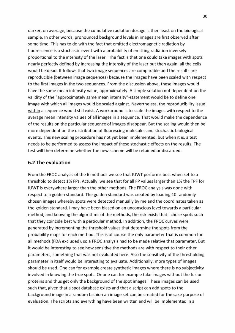
Here, we present results all of which point towards the future prospects of having a software

capable of integrating spot detection with cell segmentation. Figure 17 shows an overlay

between detected spots and segmented cells. The images of the cells were taken with an

EM-CCD camera using an exposure time of 100 ms, a 514nm laser as the light source and an

intensity at 150 W/cm2 . The cells themselves were confined in microscopic traps with spatial

dimensions (x=40 µm , y=40 µm and z=0.9 µm) constructed in a micro-fluidic chamber

(Fig.18). The height of the traps were deliberately set to z in order to ensure a monolayer of

cells. One achieves maximum cell-cell delineation with mono-layers which is a desirable trait

in images in which cells are to be segmented.

Fig.17 Overlay between segmented cells and Fig.18 An illustration of the micro-fluidic chamber

detected spots. The length of the cells where growing cells are confined in traps.

are on average 2μm and width 0.5μm.

By taking a time-lapse series of living cells in a micro-fluidic chamber one needs not only

achieve segmentation but also tracking. This is current work in progress but we show a

27

preview of what lies in store for the near future in figure.19. The tracking procedure is

illustrated in the form of a tree where the root of the tree represent a cell (the mother cell)

at time t=0. The cell was tracked for 3 generations. The histograms depicted at the lines

corresponds to intensity value distributions of the spots detected in the cell.

Fig.19 A tree diagram depicting the division of a cell during 3 generations. The blue histograms shows the distribution of

spots in each cell as a function of time. Where there are none blue histograms (Three daughter cells in the 3rd

generation) there are no spots. This kind of graphical information can be obtained by combining spot detection,

cell segmentation and cell tracking.

Another result was obtained from an experiment devised to study the interaction between

LacI and O1sym in a genetically modified E.Coli strain. O1sym is a high affinity operator, thus

we ensure that it’s being occupied by LacI most of the time. As it happens, the spots

detected with this system were drastically different from the “conventional” data. Therefore

a spot filtration script was designed to act on the detected spots from one of the seven

methods in BlobPalette3. The filtration script works by fitting a Gaussian function (Fig.21) for

each detected spot whereby the fitresults for each spot was saved. The fitresults contain the

variance and the intensity of each fitted Gaussian. By putting in the fitresults in a conditional

statement we were able to discard spots which did not fit to the ideal intensity and variance

values. The results are illustrated in Fig.20.

28

Fig.20 To the left: The detected spots after filtering out the initial result from IUWT. #Spots detected = 187

To the right: A “golden standard” where the spots were manually annotated. #Spots = 182

Fig.21 An example of a Gaussian function fitted to a spot in order to filtrate the results.

Lastly, a bleaching experiment was performed using 3 cell colonies, each continuously

exposured by laser with an intensity of 150W/cm2 during 60s. The time delay between

consecutive frames were 100ms thus we took 600 spot images of each colony. The spots

were detected using IUWT, ld=.0025, kd=3, Levels = 2, Coefficient selection = Jeffrey. The

plots for the 3 colonies are shown in Fig.22.

29

Fig.22 A bleaching experiment performed on 3 different colonies. The dotted line intersect at t=4 seconds

at which time approximately 75% of the spots have disappeared.

6 Discussion

6.1 Dealing with the noise variability between images

A software was created giving the user the chance from choosing between 7 methods for

spot detection. The reason for having many methods instead of one which is “superior” is

because superiority is measured relative the characteristics of the images. The methods are

evaluated in section 3, and are evaluated based on a set of fluorescence microscopy images.

The particular noise pattern existent in the images and the spot appearance is defined by a

combination of environmental factors, stochastic biological events and the electronics of the

imaging system. Even between images in a multi acquisition session, the noise pattern and

spot appearance varies. In fact, a method of manipulating the input images was devised in

order to minimize this variation. The idea is taking the ratio between the mean intensity

value of the first image in a sequence with the mean intensity value of all the other images.

Given an image sequence of length N, we compute N-1 ratios, each ratio associated with one

of the N-1 images. The image k in the N-1 image sequence is multiplied by its ratio, thus

elevating its pixel values if its mean intensity value is smaller than the mean intensity value

of the first image in the N sequence and vice versa. In conclusion, the first image in sequence

N dictates the intensity value tuning of the following N-1 images. On one hand this process

improves our spot detection results but on the other it shatters the reproducibility criterion.

Because given the same image sequence, the results would be dependent on which image

appears first. Although we realize this and the fact that there seems to be a tradeoff

between reproducibility and fraction of true spots detected we chose to adopt this method.

We came to the conclusion that the first image in a multi-acquisition session will always be

30

darker, on average, because the cumulative radiation dosage is then least on the biological

sample. In other words, pronounced background levels in images are first observed after

some time. This has to do with the fact that emitted electromagnetic radiation by

fluorescence is a stochastic event with a probability of emitting radiation inversely

proportional to the intensity of the laser. The fact is that one could take images with spots

nearly perfectly defined by increasing the intensity of the laser but then again, all the cells

would be dead. It follows that two image sequences are comparable and the results are

reproducible (between image sequences) because the images have been scaled with respect

to the first images in the two sequences. From the discussion above, these images would

have the same mean intensity value, approximately. A simple solution not dependent on the

validity of the “approximately same mean intensity”-statement would be to define one

image with which all images would be scaled against. Nevertheless, the reproducibility issue

within a sequence would still exist. A workaround is to scale the images with respect to the

average mean intensity values of all images in a sequence. That would make the dependence

of the results on the particular sequence of images disappear. But the scaling would then be

more dependent on the distribution of fluorescing molecules and stochastic biological

events. This new scaling procedure has not yet been implemented, but when it is, a test

needs to be performed to assess the impact of these stochastic effects on the results. The

test will then determine whether the new scheme will be retained or discarded.

6.2 The evaluation

From the FROC analysis of the 6 methods we see that IUWT performs best when set to a

threshold to detect 1% FPs. Actually, we see that for all FP values larger than 1% the TPF for

IUWT is everywhere larger than the other methods. The FROC analysis was done with

respect to a golden standard. The golden standard was created by loading 10 randomly

chosen images whereby spots were detected manually by me and the coordinates taken as

the golden standard. I may have been biased on an unconscious level towards a particular

method, and knowing the algorithms of the methods, the risk exists that I chose spots such

that they coincide best with a particular method. In addition, the FROC curves were

generated by incrementing the threshold values that determine the spots from the

probability maps for each method. This is of course the only parameter that is common for

all methods (FDA excluded), so a FROC analysis had to be made relative that parameter. But

it would be interesting to see how sensitive the methods are with respect to their other

parameters, something that was not evaluated here. Also the sensitivity of the thresholding

parameter in itself would be interesting to evaluate. Additionally, more types of images

should be used. One can for example create synthetic images where there is no subjectivity

involved in knowing the true spots. Or one can for example take images without the fusion

proteins and thus get only the background of the spot images. These images can be used

such that, given that a spot database exists and that a script can add spots to the

background image in a random fashion an image set can be created for the sake purpose of

evaluation. The scripts and everything have been written and will be implemented in a

31

future evaluation of the methods. The idea I have for a future evaluation is illustrated in the

scheme given in Fig.23. Also, the reason for the exclusion of FDA from the evaluation is that

it does not have any thresholding parameter. There are plans for introducing a threshold

such that the user may fine-tune the results. In addition, FDA can then be evaluated in a

FROC analysis and its performance compared to the other methods.

Fig.23 A scheme depicting future method analysis idea.

7 Conclusion and Future Perspectives

The path in going from posing a biological question, to performing an experiment, to the

analysis of the data from the experiment in order to answer that question, is a path in which

spots need to be detected at some intermediary step. Some example questions which

ultimately lead to spot detection are; how are transcription factors distributed in the cell at

each specific time, and are regulatory sRNAs (small RNAs) localized to their targets in the cell

or are the homogenously distributed. In unraveling the underlying biology from the spot

detection, the spots need to be detected in an accurate, unbiased and reproducible way.

Therefore a GUI-based, user friendly, spot detection software has been designed. There are

currently 7 methods implemented of which IUWT (Isotropic Undecimated Wavelet

Transform) performs best for our images having a SNR 2.6. In addition to the loading of

images and detecting the spots, the software is capable of synchronizing with μManager.

μManager is a software package for automatic control of microscopes. Thus, the

synchronization option let us detect spots and analyze the spot data in real time during the

image acquisition process. In combination with a segmentation and tracking solution, there

exists power to unravel some of the mysteries of life. One needs to be aware though that

the spot detection methods are not perfect. Therefore the software has been designed at

the code level such that new, improved, future methods may be added with relative ease.

8 Related sub-project

This section describes a project which is not part of the spot detection project per se. The

project is connected to the microscope with which we acquire spot images, thus it’s

described here. The project is the design of a GUI-based software with which we can control

32

the image acquisition process more freely than µManager allow us to do. It is written in

BeanShell which is a shell scripting language based on the Java language.

1. Here you select the name with which all image names will start with.

2. Select the channels and corresponding color. In this particular case the first channel

selected, Coherent-514 (YFP), corresponds to images taken at 514nm (i.e.

fluorescence images). The second channel, Scion-Dialamp, is the Phase channel. The

colors associated with the channels are useful for when making overlays between

images.

3. Load a position list. A position list is a set of predefined (x,y)-coordinates defining at

what positions the camera moves to. The position list is acquired in the Multi-D

Acquisition setting in µManager.

4. Set the path to where the images during the acquisition process are saved.

5. Set how many z samples the camera will take. This is as of yet a dummy-function. In

other words it is non functional. Nevertheless, it was incorporated if the need should

arise in the future to sample along the z-coordinate (the depth of the sample).

6. Define how many frames you wish to acquire.

7. Define the interval in between snapped frames.

8. Mode selection

33

8.1 Time-Channel-Position(“Trace”). Given 10 frames, 2 channels (C1 & C2) and 4

positions (A,B,C &D) the camera takes a snapshot at A using C1, then B using C1

all the way up to D using C1. Here the channel is switched to C2 and the path is

retraced back to A (D->C->B->A). Subsequently the channels are switched back to

C1 and the pattern is repeated.

8.2 Time-Position-Channel. Given the same conditions as in 8.1 the camera takes a

snapshot at A using C1 followed by a snapshot at A using C2. The position is then

changed to B and the pattern is repeated.

8.3 Position-Time-Channel. Given the same conditions as in 8.1 the camera

alternates between the channels at position A, for each channel taking an image.

Thus we will produce 10 frames taken with C1 and 10 frames taken with C2 at

position A. The position is then switched to B and the pattern is repeated.

8.4 Time-Channel-Position. Assume the same conditions as in 8.1. The camera

behaves exactly like described in 8.1 except at D. The path is not traced back in

this case; it goes like D->A->B->C->D->…

9. Set the name of the channel group. The name can be found or set in µManager.

10. Define a delay before the image acquisition takes place. Usually, one needs to wait

for a certain cell density in the micro-fluidic chamber before starting the image

acquisition process. With the initial delay property, one can circumvent the waiting

for the cells to grow.

11. A box where each element corresponds to a Channel-Position pair. The numerical

value is the exposure you wish to set for a specific pair. The row dimension is where

the channels are ordered in the way they were selected (2.). The column dimension

defines the positions.

12. Define the waiting period between every round A->B->C->D.

13. A boolean matrix defining if a snapshot is to be taken at a certain time in a certain

position using a certain channel. A numerical 1 means take a snapshot. Given the

same conditions as in 8.1 the rows are defined as : 1st Row: C1-A, 2nd Row: C1-B 3rd

row: C1-C, 4th row: C1-D, 5th row: C2-A, etc. Of course, given an acquisition with 400

frames, a way of repeating the matrix along the frame dimension must exist.

14. Set the number of frames for which the pattern is unique with respect to the frame

dimension. The unique pattern will repeat itself along the frame dimension.

15. A quick way of setting all elements to one.

16. This setting is for repeating a pattern along the vertical dimension. This feature

comes in handy when having many positions. LPRU stands for Least Position

Repeating Unit.

17. Set the number of rows for which the pattern is to be repeated vertically.

18. Pressing this button will start the image acquisition session.

34

9 References

1. Smal* I, Loog M, Niessen W and Meijering E, “Quantitative Comparison of Spot Detection Methods in Fluorescence

Microscopy”, IEEE Transactions On Medical Imaging, vol.29, no.2, pp. 282-301, 2010.

2. Fisher R.A, “The use of multiple measurements in taxonomic problems”, Annals of Eugenics, vol. 7, pp. 179-188, 1936.

3. Gonzalez R.C and Woods R.E, 2008 , Digital Image Processing, Pearson, New Jersey, 954 p.

4. Lina L, Bingyang L, Lisheng L, Buhong L, and Shusen X , “Discriminant analysis for classification of colonic tissue

autofluorescence spectra”, Optics in Health care and Biomedical Optics IV, vol.7845, pp.78450P, 2010.

5. Krzanowski W.J, “The Performance of Fisher’s Linear Discriminant Function Under Non-Optimal Conditions”,

Technometrics, vol.19,no.2, pp. 191-200, 1977.

6. Liu Q, Zhu Y, Wang B, and Li Y , “Identification of β-barrel membrane proteins based on amino acid composition

properties and predicted secondary structure”, Computational Biology and Chemistry, vol. 27, no. 3, pp. 355-361, 2003

7. Garcia-Allende P.B, Conde O.M, Mirapeix J, Cobo A, and Lopez-Higuera J.M, “Quality control of industrial processes by

combining a hyperspectral sensor and Fisher’s linear discriminant analysis”, Sensors and actuators B-chemical, vol. 129, no.

2, pp. 977-984, 2008.

8. Olivo-Marin JC, “Extraction of spots in biological images using multiscale products”, Pattern Recognition, vol.35, no.9,

pp.1989-1996, 2002.

9. Starck JL, Murtagh F, “Astronomical image and signal processing – Looking at noise, information, and scale”, IEEE Signal

Processing Magazine, vol.18, no.2, pp. 30-40, 2001

10. Starck JL, Fadili J, Murtagh F, “The undecimated wavelet decomposition and its reconstruction”, vol. 16, no. 2, pp. 297-

309, 2007.

11. Chang SG, Yu B, Vetterli M, “Adaptive wavelet thresholding for image denoising and compression”, IEEE Transactions on

Image Processing, vol. 9, no. 9, pp. 1532-1546, 2000.

12. Garcia C, Tziritas G, “Face Detection Using Quantized Skin Color Regions Merging and Wavelet Packet Analysis”, IEEE

Transactions On Multimedia, vol. 1, no. 3, pp. 264-277, 1999.

13. Starck JL, Murtagh F, Bijaoui A, “Multiresolution support applied to image filtering and restoration”, Graphical Models

And Image Processing, vol. 57, no. 5, pp. 420-431, 1995.

14. Johnstone IM, Silverman BW, “Wavelet threshold estimators for data with correlated noise”, Journal of the royal

statistical society series B-statistical methodology, vol. 59, no. 2, pp. 319-351, 1997.

15. Jansen M, Bultheel A, “Multiple wavelet threshold estimation by generalized cross validation for images with correlated

noise”, IEEE Transactions On Image Processing, vol. 8, no. 7, pp. 947-953, 1999.

16.Yoshitaka K, Norio B, Nobuhiro M, “Extended morphological processing: a practical method for automatic spot detection

of biological markers from microscopic images”, BMC Bioinformatics, vol. 11, pp. article no. 373, 2010.

17. Charles E. M, “Reciever Operating Characteristic Analysis: A Tool for the Quantitative Evaluation of Observer

Performance and Imaging Systems”, J Am Coll Radiol, vol. 3, pp. 413-422, 2006.

18. Li G, Elf J, “Single molecule approaches to transcription factor kinetics in living cells”, FEBS Letters, vol. 583, no. 24, pp.

3973-3983, 2009.

19. Kolb A, Busby S, Buc H, Garges S, and Adhya S, “Transcriptional Regulation by CAMP and its Receptor Protein”, Annual

Review of Biochemistry, vol. 62, pp. 749-795, 1993

35

20. Chen Y, Muller JD, So PTC, Gratton E, “The photon counting histogram in fluorescence fluctuation spectroscopy”,

Biophysical Journal, vol. 77, no.1, pp. 553-567, 1999.

21. Oberholzer M, Ostreicher M, Christen H, and Bruhlmann M, “Methods in quantitative image analysis”, Histochemistry

and Cell Biology, vol. 105, no. 5 , pp. 333-355, 1996.

22. Bright D. S. and Steel E. B., “Two-dimensional top hat filter for extracting spots and spheres from digital images,” J. Microsc., vol. 146, no. 2, pp. 191–200, 1987. 23. Allalou A, Pinidiyaarachchi A, Wahlby C, “Robust Signal Detection in 3D Fluorescence Microscopy”, Cytometry part A, vol. 77A, no. 1, pp. 86-96, 2010.