Automated analysis of quantitative image data using ... · from any application, ... In 2D gel...

The Annals of Applied Statistics2011, Vol. 5, No. 2A, 894–923DOI: 10.1214/10-AOAS407© Institute of Mathematical Statistics, 2011

AUTOMATED ANALYSIS OF QUANTITATIVE IMAGE DATA USINGISOMORPHIC FUNCTIONAL MIXED MODELS, WITH

APPLICATION TO PROTEOMICS DATA

BY JEFFREY S. MORRIS1,2,3, VEERABHADRAN BALADANDAYUTHAPANI1,RICHARD C. HERRICK1, PIETRO SANNA2 AND HOWARD GUTSTEIN1,2

University of Texas MD Anderson Cancer Center, University of Texas MDAnderson Cancer Center, University of Texas MD Anderson Cancer Center,

Scripps Research Institute and University of Texas MD Anderson Cancer Center

Image data are increasingly encountered and are of growing importancein many areas of science. Much of these data are quantitative image data,which are characterized by intensities that represent some measurement ofinterest in the scanned images. The data typically consist of multiple imageson the same domain and the goal of the research is to combine the quan-titative information across images to make inference about populations orinterventions. In this paper we present a unified analysis framework for theanalysis of quantitative image data using a Bayesian functional mixed modelapproach. This framework is flexible enough to handle complex, irregularimages with many local features, and can model the simultaneous effects ofmultiple factors on the image intensities and account for the correlation be-tween images induced by the design. We introduce a general isomorphic mod-eling approach to fitting the functional mixed model, of which the wavelet-based functional mixed model is one special case. With suitable modelingchoices, this approach leads to efficient calculations and can result in flexi-ble modeling and adaptive smoothing of the salient features in the data. Theproposed method has the following advantages: it can be run automatically,it produces inferential plots indicating which regions of the image are associ-ated with each factor, it simultaneously considers the practical and statisticalsignificance of findings, and it controls the false discovery rate. Although themethod we present is general and can be applied to quantitative image datafrom any application, in this paper we focus on image-based proteomic data.We apply our method to an animal study investigating the effects of cocaineaddiction on the brain proteome. Our image-based functional mixed modelapproach finds results that are missed with conventional spot-based analy-sis approaches. In particular, we find that the significant regions of the image

Received December 2009; revised May 2010.1Supported by National Cancer Institute (CA-107304).2Supported by National Institute for Alcohol Abuse (AA-016157).3Supported by Statistical and Applied Mathematical Sciences Institute (SAMSI) Program on

Analysis of Object Data (AOD).Key words and phrases. Bayesian analysis, false discovery rate, functional data analysis, func-

tional mixed models, functional MRI, image analysis, isomorphic transformations, proteomics, 2Dgel electrophoresis, wavelets.

894

http://www.imstat.org/aoas/

http://dx.doi.org/10.1214/10-AOAS407

http://www.imstat.org

ISO-FMM FOR IMAGE DATA 895

identified by the proposed method frequently correspond to subregions of vis-ible spots that may represent post-translational modifications or co-migratingproteins that cannot be visually resolved from adjacent, more abundant pro-teins on the gel image. Thus, it is possible that this image-based approachmay actually improve the realized resolution of the gel, revealing differen-tially expressed proteins that would not have even been detected as spots bymodern spot-based analyses.

1. Introduction. Image data are increasingly encountered in many areas ofscience and technology, including medicine, defense, robotics, security, and ma-terials science. Image analysis involves the extraction of meaningful informationfrom these data.

Some types of image analysis are performed subjectively by an expert user whois trained to visually extract the important features from the image. For example,a trained radiographer may inspect a CT scan to determine whether a patient hasa tumor, or a trained pathologist may look at a scanned microscopic slide anddetermine the histology of a tumor. Other types of image information can be auto-matically extracted using a computer-based analysis of the digitized image basedon an expert systems approach. For example, face recognition software can be usedto identify an individual in an image, or optical character recognition software canbe used to ascertain license plate numbers from still images taken at a toll booth.In these examples, the data are digitized and pattern recognition is used to performdiscrimination, but the analysis is still qualitative in nature because the informationof interest is the presence or absence of particular features in the image, not themagnitudes of the pixel intensities themselves.

In other image data, the magnitudes of the digitized pixel intensities actuallyrepresent an approximate quantification of some measurement of interest. For ex-ample, in functional magnetic resonance imaging (fMRI), magnetic images are ob-tained for serial slices of the brain, and the pixel intensities represent the amountof oxygenated blood flow to that part of the brain, which is a surrogate measurefor the brain activity level. In 2D gel electrophoresis (2-DE)-based proteomics,the proteomic content of a biological sample is physically separated on a two-dimensional polyacrimidic gel by its isoelectric point (pH) and molecular mass.The gel is scanned to produce an image characterized by spots that correspond toproteins present in the sample. The intensities of the spots are rough measures ofprotein abundance. We refer to this type of image data as quantitative image data(QID), which is the primary focus of this paper.

A set of QID typically involves multiple scanned images from the same indi-vidual and/or from different individuals, with intensities observed over the sametwo-dimensional (or higher) domain. The overall goal of this type of quantitativeimage analysis (QIA) is to combine information across images to make statisticalinferences about populations or about the effects of certain interventions on thepopulations represented in the images. One important specific goal of QIA is to

896 J. S. MORRIS ET AL.

identify which regions of the image differ significantly across treatment groupsor populations. For example, in fMRI we might analyze images from individualsperforming various functions in order to determine which parts of the brain aretypically active during each activity, or we might wish to distinguish between dif-ferent populations of patients with respect to their brain activity during a givenactivity, for example, in response to visual stimulus for children with and withoutattention deficit disorder. In proteomics, we aim to find which regions of the gel,and thus which proteins, are differentially expressed between cases and controls ina case-control study.

These image data sets are enormous in size and complex in nature, presentingnumerous challenges in terms of storing, managing, analyzing and viewing thedata. It is not uncommon to have hundreds or thousands of images in a given dataset, with each image sampled on a grid of tens of thousands to millions of pixels.Managing and viewing data sets of this size is difficult; performing rigorous sta-tistical analyses on the data is particularly challenging. Before statistical analysiscan be performed, the raw, digitized images must undergo a number of processingsteps, including alignment, background correction, normalization, denoising andartifact removal. These steps may involve technology-specific methods, and mustbe done before any further analysis takes place. We will not discuss preprocess-ing methods in detail in this paper, but will assume the researchers have appliedsuitable processing methods to the data before using the QIA methods we describe.

Feature extraction vs. image-based modeling: Researchers frequently use a fea-ture extraction approach to analyze QID. They are motivated by the premise thatthe relevant information in the images is contained in well defined, discrete fea-tures that can be extracted by computing numerical summaries according to theirestimated feature structure. The steps of a feature extraction approach are to iden-tify the salient features in the images, quantify each feature for each individual,and then use standard univariate and multivariate statistical methods to determinewhich features are associated with the factors of interest. For example, in fMRI,the preprocessed pixel intensities can be integrated within predefined Regions ofInterest (ROI), for example, brain regions, and then these regions can be analyzedto determine which regions are related to the underlying activity or population.In 2-DE proteomics, a spot-detection algorithm estimates distinct protein spots inthe images. The protein spots are quantified and then surveyed to determine whichare differentially expressed. This approach is computationally efficient because itreduces the data from complex, high-dimensional images to a vector of spot inten-sities, and can retain the relevant information contained in the QID, provided thatall the salient features are properly detected and quantified.

The problem with this approach is that any information in the image not con-tained in one of the feature summaries will be completely lost to the analysis. InfMRI, there may be important differences within subregions of the predefined re-gions of interest that could be missed by integrating the entire region. In 2-DE,spot detection methods are not perfect and may fail to detect some differentially


expressed proteins as distinct spots. One of the inherent dangers of this problem isthat the researchers may never be aware that they missed anything—that there wasinformation of significance in their data that was missed because of inadequatefeature extraction.

An alternative to feature extraction is to model the images in their entirety us-ing a suitable statistical modeling framework, which is a challenging endeavorwe call an image-based modeling approach. To be appropriate for image-basedmodeling, an analytic method must possess the following three major character-istics: (1) sufficient flexiblity and adaptability to accommodate the local featuresthat tend to characterize these complex, irregular data; (2) the ability to appropri-ately borrow strength spatially across the image; and (3) enough computationalefficiency to be feasibly applied to data sets of this magnitude. Some examplesof recently published image-based modeling methods include those of Reiss andOgden (2009), who constructed a generalized linear model method for image pre-dictors, and Smith and Fahrmeir (2007), who analyzed fMRI data using Bayesianvariable selection on image pixels and an Ising prior to model spatial correlationamong the variable selection parameters. QID can be viewed as functional datawith the two-dimensional domain given by the rows and columns of the image andthe range given by the pixel intensities, and thus can be analyzed using a functionaldata analysis [FDA, Ramsay and Silverman (1997)] approach.

Recent work on Functional Mixed Models (FMM) [Guo (2002), Morris et al.(2003), Morris and Carroll (2006), Morris et al. (2006), Morris et al. (2008)] pro-vides a general modeling framework useful for modeling many types of functionaldata, but has not yet been adapted for use with image data. In this paper we presenta unified, Bayesian image-based analysis approach for QID based on a version ofthe FMM suitable for higher dimensional image data. The model fitting is doneusing an isomorphic transformation approach, which we define and introduce inSection 3.2. The method can simultaneously model the effects of multiple factorson the images through fixed effects and can account for correlations between im-ages that are induced by the design through random effect modeling. The isomor-phic modeling approach results in efficient calculations and, with suitable trans-formation, can accommodate nonstationary features in the covariance matrices,and result in adaptive smoothing and borrowing of strength across pixels in eachdimension while the inference is performed. The method yields posterior proba-bilities of specified effect sizes that can be interpreted as local false discovery rates[FDR, Benjamini and Hochberg (1995), Storey (2003)]. The posterior probabili-ties can be used in Bayesian inference to flag regions of the curves as significantwhile considering both practical and statistical significance and controlling theFDR. The software to implement this method can be run automatically with littleuser input, and is efficient enough to handle even very large image data sets. Al-though this method is generally applicable to all QID, in this paper we focus on2-DE data. We show that this adaptive, image-based approach can find results that


would have been missed with standard spot-level analyses, and may extract moreprotein information from the gels than was previously known to be present.

In Section 2 we discuss image-based proteomics and standard analysis ap-proaches, and introduce the brain proteomics data set that we consider in this paper.In Section 3 we describe the methodology: we overview functional mixed models,describe our general isomorphic approach to model fitting, and present the isomor-phic functional mixed model for higher dimensional image data. Also, we describehow to conduct Bayesian FDR-based inference using the output data and presentan image compression approach that can be used optionally to speed up calcu-lations. In Section 4 we apply this method to the brain proteomics data set andcompare and contrast results with a feature extraction approach. We finish with adiscussion of the implications of our results for 2-DE proteomics and as a generalmethodology for quantitative image data analysis in Section 5.

2. Image-based proteomics data.

2.1. Introduction to proteomics. Over the past two decades, advances in ge-nomics have fueled increased interest in the field of proteomics. Proteomics dif-fers from genomics in that the former field involves the direct measurement ofproteins rather than their precursors, genes and messenger RNA. Our focus is onthe use of proteomics for biomarker discovery, which involves the measurementof the relative abundance of proteins across different samples to determine whichare differentially expressed across groups or correlated to a factor of interest. Theproteins of interest can then be validated and further studied for possible clinicalapplications, for example, for early detection of cancer or as markers of responseto a particular cancer therapy. Various types of proteomics data can be consid-ered quantitative image data, including liquid chromatography–mass spectrometry(LC–MS) and 2D gel electrophoresis (2-DE).

While LC–MS is growing in importance, the major workhorse in biomarker dis-covery proteomics to date has been 2-DE. The process of 2-DE involves stainingand denaturing the biological sample, running it through a polyacrimidic gel, andseparating the proteomic content of the sample by isolectric point (pH) and thenby molecular mass. The gel is then digitally scanned to produce an image of thestained spots that correspond to proteins present in the sample, which are doubleindexed by their molecular mass and pH. The spots on the gel physically con-tain the actual proteins, so protein identification is easily accomplished by cuttingout the spot, enzymatically digesting it, and using MS–MS to ascertain its iden-tity. One variant of 2-DE that may yield more accurate relative quantifications is2D difference gel electrophoresis [DIGE, Lilley (2003), Karp and Lilley (2005)],which involves differentially labeling two samples with two different dyes, loadingthem onto the same gel, and then scanning the gel with two different lasers, eachof which specifically picks up one of the two dyes. When comparing two groups,


paired samples from each group can be run on the same gel, effectively condition-ing the gel effect out of the analysis. In more general problems, one dye (the activechannel) can be used for the primary sample and the other dye (the reference chan-nel) used on some common reference material used on all gels so that it may serveas an internal normalization factor.

2-DE has been criticized for various perceived limitations of the technology,including its limited ability to measure proteins with medium or low abundanceor to resolve co-migrating proteins with similar pH/mass combinations [Gygi etal. (2000)]. Although the technology itself may possess some technical limitations,a major factor limiting the realized potential of 2-DE is a lack of efficient andeffective algorithms to process and analyze the gel images. More effective analyticmethods that better extract proteomic information from the gel images may helpthe technology more fully realize its potential.

2.2. Spot-based analysis of 2-DE proteomic data. Nearly all existing 2-DEgels are analyzed using a feature extraction approach whereby spots are detectedand quantified for different gel images and then analyzed to ascertain which aredifferentially expressed. The success of a feature extraction approach depends onthe effectiveness of the feature detection and quantification method used and, un-til recently, the predominant approaches used for spot detection and quantificationhad major problems. Traditional approaches based on spot detection on individ-ual gels followed by matching spots across gels suffer from problems with miss-ing data, spot detection errors, spot matching errors and spot boundary estimationerrors [Clark and Gutstein (2008), Morris, Clark and Gutstein (2008)]. The abun-dance of these errors may be partially responsible for some researchers concludingthe technology is ineffective. In recent years, alternative spot detection strategieshave been developed that mitigate these errors to a degree, and include Pinna-cle, a method we have developed [Morris, Clark and Gutstein (2008), Morris etal. (2010)], and commercial packages SameSpots by Nonlinear Dynamics (New-castle upon Tyne, UK), Redfin Solo by Ludesi (Malmo, Sweden) and Delta2Dby Decodon (Greifswald, Germany). While improving from past methods, thesespot-based approaches are still far from perfect, and, in particular, still have somedifficulty resolving distinct co-migrating proteins that are present in the same spot.Thus, there may be more to gain by using an image-based modeling approach.

2.3. Image-based analysis approaches for 2-DE. Spot-based approaches arealmost universally used for the analysis of 2-DE data. We know of only one paperin the current literature that describes the application of an image-based model-ing approach. Faergestad et al. (2007) presented a pixel-based method for pairwiseanalysis of 2-DE data that involves the application of partial least squares regres-sion (PLSR) to the vectorized gel images (after preprocessing). Faergested et al.used a jacknife procedure to conduct inference, repeatedly applying the PLSR toeach leave-one-out cross-validation sample and then performing a t-test at each


pixel using the cross-validation regression coefficients as the data. In order to avoidflagging pixels that were statistically but not practically significant, they restrictedtheir attention to pixels with a certain minimum standard deviation across samples.The general image-based method we introduce in this paper is not limited to pair-wise inference; it can account for correlation among images from the same subjector batch; it performs adaptive smoothing as part of the estimation and inference;and it yields rigorous unified FDR-based Bayesian inference that simultaneouslyaccounts for both statistical and practical significance. Our method can be appliedto any type of image-based proteomics data, including LC–MS, 2-DE and DIGE.

2.4. Motivating example: Cocaine addiction brain proteomics study. Themethods we develop in this paper are applied to proteomic data from a neuro-biology study on cocaine addiction. The study aimed to identified neurochemicalchanges in the brain that are associated with the transition from nondependent druguse to addiction. The addiction process is conceptualized as an increasing motiva-tion to seek drugs, resulting in increased drug intake, loss of control over drugintake and compulsive drug taking. Previous studies suggest that prolonged expo-sure to cocaine or opiate drugs leads to increased self-administration and a pro-nounced elevation in reward thresholds [Leith and Barrett (1976), Kokkinidis,Zacharko and Predy (1980), Markou and Koob (1992), Schulteis et al. (1994)].Neurochemical changes in parts of the basal forebrain structure, the extendedamygdala, parallel these decreases in the function of the reward system [Parsons,Koob and Weiss (1995), Weiss et al. (1992), Heinrichs et al. (1995), Richter andWeiss (1999)]. These data suggest that substance dependence or addiction pro-duces a pronounced dysregulation of the brain’s reward systems, and that neu-rochemical changes in the extended amygdala may provide a substrate for suchdysfunction. The neurochemical changes may involve cellular effects at the trans-lational and post-translational levels that alter protein expression and function, andthus may be detected by proteomic analysis.

An animal study to investigate these concepts used a model developed byAhmed and Koob (1998). The animal model was based on rats that were trainedto obtain cocaine by pressing a lever. Six rats were given short durations ofdrug access (1 hour/day), and 7 rats were given long durations of drug access(12 hours/day). The study included 8 control rats. The rats were eventually euth-anized, and their brain tissue was harvested and microdissected to extract variousregions of the extended amygdala. Tissues from the brain samples were then sub-jected to 2-DE to assess their proteomic content. The goal was to compare andcontrast protein expression and modification associated with excessive levels ofcocaine intake and to compare tissues from animals given long versus short accessto the drug. The data we analyzed for this paper were obtained from the the centralnucleus region of the extended amygdala. The data set contains a total of 53 gelsfrom 21 rats, with roughly 2–3 gels per rat.


3. Methods. In this section we review previous work on functional mixedmodels and wavelet space modeling for 1D functional data, and then discuss howthis approach can be used with other transformations, that is, not just wavelets.Thereafter, we describe how to adapt this method to model image data and discusshow to perform rigorous FDR-based Bayesian inference from its output.

3.1. Functional mixed models and wavelet-based modeling. For background,here we describe the wavelet-based functional mixed models method (WFMM) ofMorris and Carroll (2006). Suppose we observe a sample of N curves Yi(t), i =1, . . . ,N , each defined on a compact set T . The FMM is given by

Y(t) = XB(t) + ZU(t) + E(t),(1)

where Y(t) = {Y1(t), . . . , YN(t)}′ is a vector of observed functions, “stacked”as rows. Here, B(t) = {B1(t), . . . ,Bp(t)}′ is a vector of fixed effect functionswith corresponding N × p design matrix X, U(t) = {U1(t), . . . ,Um(t)}′ is a vec-tor of random effect functions with corresponding N × m design matrix Z,and E(t) = {E1(t), . . . ,EN(t)}′ is a vector of functions representing the resid-ual error processes. The effect functions measure the partial effect of the cor-responding covariate at position t of the functions. The set of random effectfunctions U(t) is a realization from a (mean zero) multivariate Gaussian processwith m × m between-function covariance matrix P and within-function co-variance surface Q(t1, t2), denoted by U(t) ∼ M G P(P,Q) and implying thatcov{Ub(t1),Ub′(t2)} = Pbb′Q(t1, t2). The residual errors are assumed to followE(t) ∼ M G P(R,S), independent of U(t). The random effect or residual error por-tions of the model can be stratified to allow covariances indexed by some factor,ZU(t) = ∑H

h=1 ZhUh(t) with Uh(t) ∼ M G P(Ph,Qh) or E(t) = ∑Cc=1 VcEc(t)

with Vc a vector whose ith element is 1 if curve i is from stratum c and Ec ∼M G P(Rc, Sc).

In practice, observed functional data are sampled on some discrete grid. Assum-ing all observed functions are sampled on the same fine grid t = (t1, . . . , tT ), thediscrete version of (1) is

Y = XB + ZU + E,(2)

where Y is an N × T matrix of observed curves on the grid t, B is a p × T

matrix of fixed effects, U is an m × T matrix of random effects, and E is anN × T matrix of residual errors. Following Dawid (1981), U follows a matrixnormal distribution with m × m between-row covariance matrix P and T × T

between-column covariance matrix Q, which we denote by U ∼ M N (P,Q), im-plying cov(Uij ,Ui′j ′) = Pii′Qjj ′ . The residual error matrix E is assumed to beM N (R,S). The within-random effect curve covariance surface Q and residualerror covariance surface S are T × T covariance matrices that are discrete approx-imations of the corresponding covariance surfaces in T × T .


Morris and Carroll (2006) used a wavelet basis modeling approach to fit themodel (2), which involves three steps. First, a fast algorithm called the discretewavelet transform [DWT, Mallat (1989)] is applied to each of the N observedfunctions on grid t to yield a vector of T wavelet coefficients for each function,effectively rotating the data axes to transform the data into the wavelet space. Sec-ond, a Markov chain Monte Carlo (MCMC) procedure is used to obtain posteriorsamples from a wavelet-space version of model (2). The wavelet-space covariancematrices for the random effect functions and residual errors are modeled as diago-nal, but with different variances for each wavelet coefficient, and spike-slab priorsare assumed on the fixed effects’ wavelet coefficients. These assumptions are par-simonious, yet accommodate nonstationary features in the data-space covariancematrices Q and S and induce adaptive regularization of the fixed and random effectfunctions, Ba(t) and Ub(t) [Morris and Carroll (2006)]. Third, the inverse DWT isapplied to the the posterior samples of the wavelet-space parameters to yield pos-terior samples of the parameters in the data-space model (2), which can be used toperform Bayesian inference.

3.2. Isomorphic modeling of functional mixed models (ISO-FMM). TheWFMM is just one example of a general approach to fitting functional mixedmodels we call an isomorphic approach (ISO-FMM), which we introduce here.The same basic three-step approach underlying the WFMM can be applied us-ing isomorphic transformations not involving wavelets if desired. We define anisomorphic transformation as one that preserves all of the information in the orig-inal data, that is, is invertible. More precisely, given row vector y ∈ �(T), wesay a transform f :�(T ) → �(T ) is isomorphic if there exists a reverse trans-form f −1 such that f −1{f (y)} = y. The wavelet transform is isomorphic becauseIDWT(DWT(y)) = y, but isomorphic transformations can be constructed in otherways as well, for example, by using other basis functions including Fourier bases,spline bases and certain empirically determined basis functions like functionalprincipal components.

Suppose we observe N functions all on the same fine grid t of length T , result-ing in N ×T data matrix Y whose rows are the observed functions and columns in-dex the grid locations. The following steps describe the general steps of a Bayesianimplementation of the ISO-FMM for functional data:

1. Transform each of the rows of Y using an isomorphic transformation f , repre-sented as D = f (Y ), with f (·) applied to a matrix implying here the transformf is applied separately to each row. Rather than indexing positions within thecurve, the columns of D will index items in the transformed space, for exam-ple, basis coefficients. We can think of the induced functional mixed model inthe transformed space with the columns of D,B∗ = f (B),U∗ = f (U), andE∗ = f (E) indexing coefficients in the alternative space. We refer to this as thetransformed-space FMM.


2. Apply an MCMC procedure to the transformed-space FMM to obtain posteriorsamples of all of its parameters. This requires specification of (a) parsimoniousassumptions on the covariance matrices Q∗ and S∗ that are sufficiently flexibleto capture important features of Q and S, and (b) a prior distribution on thefixed effects in the transformed-space FMM to induce effective regularizationof the fixed effect functions B∗.

3. Apply the inverse isomorphic transform f −1 to the posterior samples of thefunctional quantities in the transformed-space FMM to obtain posterior samplesfrom the original data-space FMM (2), where Bayesian inference is performed.

This approach could also be applied in a frequentist context. That would involvefitting the transformed-space model with some explicit roughness penalties in ap-propriate places, for example, the fixed and random effect functions, to induceadaptive smoothing, and then transforming the estimated quantities back to thedata space. This would easily yield estimates, but more work would need to bedone to obtain inferential quantities.

The use of an isomorphic transformation ensures that the representation in thetransformed data retains all of the information contained in the original data, thatis, is “lossless,” and thus any basis coefficients can be considered as transformedraw data rather than estimated parameters. Thus, the transformed-space model isisomorphic to the data-space model. This allows us to perform the modeling in thetransformed space, where it may be possible to perform modeling and regulariza-tion more parsimoniously and conveniently, and yet obtain valid inference in thedata-space model, where the parameters are more clearly interpretable.

For many isomorphic transformations, it is possible to assume parsimoniousstructures for Q∗ and S∗ in the basis space and still accommodate a rich class ofstructures for data space within curve covariance matrices Q and S. For example,using a Fourier transform, any stationary covariance matrix can be representedby uncorrelated Fourier coefficients, so diagonal Q∗ and S∗ are fully justified ifwe are willing to assume stationarity in Q and S. Diagonal assumptions on Q∗and S∗ allow the transformed-space FMM to be fit one column at a time, makingthe procedure highly parallelizable and reducing the memory requirements of thesoftware. This assumption may also be justifiable in some empirically-determinedbasis spaces such as FPC. For wavelets, the whitening property of the transformmakes diagonal Q∗ and S∗ a reasonable working assumption that accommodatesmany commonly encountered nonstationary features. For a given isomorphic trans-formation, one must decide what parsimonious assumptions are reasonable in thebasis space, and carefully consider what constraints these assumptions induce inthe data space.

Another advantage of transformed-space modeling is that for many isomorphictransforms, there are natural prior distributions on basis space coefficients that caninduce regularization of the functional effects in the model and effectively act likeroughness penalties. For example, with wavelets, a sparsity prior that has a spike


at zero and medium-to-heavy tails like a spike-slab prior leads to adaptive regular-ization of the underlying effect function. Spline bases are frequently regularizedby second-order penalties, which can be induced by a Gaussian prior. First-orderpenalties can be induced by double-exponential priors.

Although orthonormal linear isomorphic transformations are convenient to usebecause they represent a simple rotation of the axes, they are not the only pos-sibility. The transform does not have to be orthonormal or even linear. With anorthonormal transform, i.i.d. white noise has the same distribution and total en-ergy in both the data and basis space, but these are not necessary properties forthe FMM. With linear transforms [f (Y ) = YW ′ for some matrix W ′], a Gaussianmodel in the data space induces a Gaussian model in the transformed space, andvice-versa, but this is also not absolutely necessary for valid modeling. For ex-ample, one could specify a Gaussian model in the transformed space that is usedfor the fitting, and this would correspond to some non-Gaussian model in the dataspace that might not have a simple closed form, but which could still be a validand reasonable data-space likelihood.

If the set of functions jointly have a very sparse representation in the chosen ba-sis space, it may be possible and advantageous to use an approximately isomorphictransformation of lower dimension that still retains almost all of the informationfor the original functions. We describe a way to perform this compression in themultiple function context in Section 3.5.

Many methods in the existing statistical literature use a basis function approachto represent functions or vectors, but rather than transformed data the coefficientsare typically treated as parameters to estimate and the transforms are not isomor-phic but lower rank projections. There are some methods in the current statisticalliterature that effectively use an isomorphic modeling approach [e.g., wavelet re-gression, Clyde, Parmigiani and Vidakovic (1998); spectral analysis of stationarytime series, Diggle and Al Wasel (1997); nonisotropic modeling of geostatisticaldata, Sampson and Guttorp (1992)]; however, to our knowledge, this has not beendiscussed previously as a general modeling strategy. Our intended contributionshere are to (1) explicitly offer an isomorphic approach as a general modeling strat-egy and (2) apply this approach to functional mixed modeling.

3.3. ISO-FMM for quantitative image data. In this section we introducea functional mixed model for image data, describe how to model image data usingour isomorphic transformed-space approach, and provide implementation detailsusing higher dimensional wavelet transforms. Even though these results hold gen-erally for higher dimensional images, we present the results for 2D images for easeof exposition.

3.3.1. Functional mixed models for quantitative image data. Suppose we havea sample of N images, Yi, i = 1, . . . ,N , with each Yi a T1 × T2 matrix contain-ing the image intensities sampled on a regular, equally-spaced two-dimensional


grid (t1, t2) with t1 = (t11, . . . , t1T1)′ and t1 = (t21, . . . , t2T2)

′. A functional mixedmodel for these image data, with (t1, t2) a coordinate on the grid, can be written as

Yi(t1, t2) =p∑

a=1

XiaBa(t1, t2) +m∑

b=1

ZibUb(t1, t2) + Ei(t1, t2),(3)

where Ba and Ub are fixed and random effect images, respectively, which mea-sure the effects of scalar fixed or random effect covariates on the correspondinglocation of the image Y , and Ei contains the residual error images. The Ub andEi are mean zero Gaussian processes defined on the surface, with correspondingbetween-image covariance matrices P and R, respectively, and four-dimensionalwithin-image covariance surfaces Q(t1, t2, t

′1, t

′2) and S(t1, t2, t

′1, t

′2) summarizes

the covariance between locations (t1, t2) (t ′1, t ′2) of the random effect and residualerror images, respectively.

Let each image be represented by a row vector of length T1 ∗T2, yi = {vec(Yi)}′,where vec is the column stacking vectorizing operator. If we let Y be theN × T (= T1 ∗ T2) matrix whose rows contain the vectorized images, then thediscrete image mixed model can be written as

Y I = XBI + ZUI + EI ,(4)

with each row of BI and UI containing one of the vectorized fixed or random ef-fect images, respectively, that measure the effect of a scalar fixed or random effectcovariate on the corresponding location of the image, and with the rows of EI con-taining the vectorized “residual error images.” The columns index the pixels in theimage. The superscript “I” simply is a reminder that these quantities are based onimages. As before, we assume that UI ∼ M N (P,Q) and EI ∼ M N (R,S), withP and R being m × m and N × N matrices defining covariances between images,and Q and S being T × T within-function two-dimensional covariance matricesfor the random effects and residuals that model the covariance between differentpositions within the images. For example, Q{t1 + (t2 − 1) ∗T1, t

†1 + (t2 − 1)† ∗T1}

describes the covariance between UIb (t1, t2) and UI

b (t†1 , t

†2 ). Note that any reason-

able structure on these within-image covariance matrices should not just model theautocovariance based on the proximity within the vector yi , but rather the proxim-ity within the higher dimensional image Y I

i , that is, in all dimensions.

3.3.2. ISO-FMM for quantitative image data. The ISO-FMM approach for1D functions described in Section 3.2 can be applied to QID, as well, using iso-morphic transforms and inverse transforms that operate on the higher dimensionalfunctions, for example, images. The covariance assumptions in the transformedspace and the regularization prior distributions should be chosen to induce ap-propriate spatial correlation, adaptive smoothing and borrowing of strength in alldimensions.


The isomorphic transform f in the image space will map the T = T1 ×T2 pixelsto a set of alternative transformed-space coefficients, DI

i = f (Y Ii ). This transform

can be constructed a number of different ways. One natural way is to take tensorproducts of suitable 1D transforms, leading to a separable transform. It is also pos-sible to use special bases constructed for image data. Depending on the resolutionof the images and transform used, computational feasibility can become an issuebecause the transform will have to be applied to all N observed images as well asto all p fixed effect images for each of M posterior samples. After transformation,a model is then proposed in the transformed space.

If the transform is linear, then the Gaussian assumptions from (4) hold in boththe data and transformed space, and our transformed-space model is given by

DI = XBI∗ + ZUI∗ + EI∗,(5)

with the rows of DI ,BI∗ = f (BI ),UI∗ = f (UI ), and EI∗ = f (EI ) containingthe transformed representations for each of the corresponding image-based quan-tities in (4), with UI∗ ∼ MN(P,Q∗) and EI∗ ∼ MN(R,S∗). As before, f (A)

for some matrix A means applying the transformation f sequentially on the rowsof A. If a separable linear transform is used, then the linear transform matrix for thevectorized images can be explicitly defined as follows. Suppose we obtain a matrixof coefficients DI

i from the sampled image Y Ii by applying a linear transform W1

to the rows of the image and W2 to the columns, that is, DIi = W1Y

Ii W ′

2. Thistransformation can be explicitly represented as di = yi W ′, where yi = vec(Y I

i )′and di = vec(DI

i ) are the vectorized image and coefficient matrix, respectively,W ′ = (W2 ⊗W1) is the linear transformation matrix, and ⊗ is the Kronecker prod-uct. This representation makes it easy to explicitly see the connections between thedata-space and transformed-space matrix models (4) and (5) for the QID context asDI = Y I W ′, BI∗ = BI W ′, UI∗ = UI W ′, and EI∗ = EI W ′, and Q∗ = W ′QWand S∗ = W ′SW . If W1 and W2 are orthogonal, then it follows that W is alsoorthogonal. These results generalize to general r-dimensional functions stacked asvectors using W ′ = (Wr ⊗ Wr−1 ⊗ · · · ⊗ W1).

3.3.3. Implementation details using wavelets. The same properties that makewavelet bases convenient for isomorphic modeling in 1D functional data (fast cal-culations, compact support, whitening property, joint frequency–time representa-tion, sparse representations for broad classes of data) also make them useful formodeling QID. Here, we will describe the implementation details for ISO-FMMusing higher dimensional wavelet transforms to construct the isomorphic transfor-mations, which involves three factors: choice of transform, specification of covari-ance structure, and regularization prior.

There are various ways to construct isomorphic transforms for image data usingwavelet bases. These transforms can be separable or nonseparable. A separable, orrectangular, transform is easily constructed by applying the 1D DWT separately


to each row and each column of the image. As mentioned in Section 3.1, after ap-plying the wavelet transform to a vector of data, the resulting wavelet coefficientsare double-indexed by scale j = 1, . . . , J and location k = 1, . . . ,Kj . If we applya separable 2D wavelet transform, each coefficient is quad-indexed by row scale j1and location k1, and column scale j2 and location k2.

Nonseparable transforms can also be used. Although they are not representedas simple tensor products of 1D transforms, they are constructed using linear op-erators, and so still represent a linear transformation. The most commonly usednonseparable wavelet transform is a square transform. This type of decompositionyields three types of wavelet coefficients at each scale j = 1, . . . , J , correspond-ing to horizontal, vertical and diagonally-oriented wavelet bases. In this case, thewavelet coefficients are triple-indexed by scale (j = 1, . . . , J ), orientation {l = 1(row details), 2 (column details), 3 (2D details)} and location (k = 1, . . . ,Kjl). Thesquare wavelet transform tends to better model local behavior and leads to moreparsimonious representations than the rectangular transform, and so is commonlyused in practice. With the basis functions aligned with the principal axes (horizon-tal, vertical and diagonal), a disadvantage of the square transform is that sometimesit does not efficiently represent smoother contours or features of the images that donot align with the principal axes [Do and Vetterli (2001)]. This leads to less effec-tive adaptive smoothing for images with these types of features. Other 2D wavelettransforms have been constructed for this purpose and could be used in place ofthe square transform, for example, curvelets [Candes and Donoho (2000)], con-tourlets [Do and Vetterli (2005)] or qincunx wavelets [Feilner, Van De Ville andUnser (2005)]. We choose to use the square nonseparable wavelet transform for2-DE data because the key features of the images, the spots, are aligned with thehorizontal and vertical axes and so should be well represented by them. We foundthem to be more efficient than the rectangular separable transform which containsmany long, thin basis functions constructed by combining a low frequency basisin one dimension (small j ) and high frequency basis in the other (large j ).

Again, motivated by the whitening property of the wavelet transform, wemodel the wavelet coefficients as independent, that is, Q∗ = diag(qjlk) and S∗ =diag(sjlk), allowing each coefficient triple-indexed by its scale j , orientation l andlocation k to have its own variance component. The independence leads to parsi-monious modeling, while the heteroscedasticity accommodates nonstationary spa-tial features in the data space matrices Q and S. In Supplementary Material, weillustrate through plots and movies [Morris (2010)] the effective spatial covariancestructures of Q and S induced by independent heteroscedastic wavelet space mod-els for our 2-DE data. It accommodates spatial covariance in all directions, basedon proximity horizontally, vertically and diagonally, and the strength of this spa-tial covariance is allowed to vary across different parts of the image. This adaptivehandling of spatial correlation is important in 2-DE, since we expect strong au-tocorrelation within spots that rapidly falls off outside of the spot, and we expecta more slowly decaying autocorrelation in nonspot background regions of the gel.


Further, the structure allows different image-to-image variances for different pix-els in the image, which is important to obtain accurate pixelwise inference, sincewe expect different protein spots to have different variances. These principles gen-eralize to higher dimensional images when the corresponding higher dimensionalDWT is used for transformation.

We assume the spike-Gaussian slab prior on the wavelet coefficients for thefixed effects, which is written as

B∗ajlk = γ ∗

ajlk N (0, τajl) + (1 − γ ∗ajlk)I0,

(6)γ ∗ajlk = Bernoulli(πajl),

with regularization parameters π and τ indexed by covariate a, scale j and orienta-tion l, and estimated from the data using the empirical Bayes procedure similar toMorris and Carroll (2006), as detailed in a supplementary article [Morris (2010)].This induces adaptive smoothing of the fixed effect images Ba(t1, t2). By index-ing the parameters by covariate, we allow for different regularization parametersfor different fixed effect images, and by indexing by scale j and orientation l, weare able to naturally accommodate different degrees of smoothness horizontally,vertically and diagonally within the fixed effect images.

After specifying vague proper priors on the variance components, we are leftwith a fully specified Bayesian model for the transformed-space FMM (2). Weuse a Markov chain Monte Carlo (MCMC) procedure to obtain posterior samplesof the transformed-space fixed effect functions B∗, and then apply the inverse 2Dwavelet transform to them to obtain posterior samples of the data-space fixed ef-fect functions B , which are used for Bayesian inference. The MCMC details arepresented in the supplementary article by Morris (2010).

3.4. Bayesian FDR-based inference. Given the posterior samples of Ba(t1, t2),the fixed effect image describing the effect of covariate Xa on the images as a func-tion of position (t1, t2), we can perform Bayesian inference to flag significant re-gions of the curves by extending the approach used in Morris et al. (2008), asfollows.

First, we must define the effect size that is of practical significance, say, δ.For example, if the image intensities are modeled on a log2 scale, then δ = 1would correspond to a two-fold difference. From the posterior samples of B , wecan compute the posterior probability of an effect size of at least δ, pδ

a(t1, t2) =Prob{|Ba(t1, t2)| > δ}, which can be plotted in what we call a probability discov-ery image, and define significant regions of the image as those with pδ

a(t1, t2) > φ

for some threshold φ. The quantities 1 − pδa(t1, t2) can be considered q-values,

or estimates of the local false discovery rate [Storey (2003)], as they measure theprobability of a false positive if position (t1, t2) is called a “discovery,” defined asa region in the image with at least δ effect size.


The significance threshold φ can be determined using classical Bayesian utilityconsiderations such as those of Mueller et al. (2004) based on the elicited rela-tive costs of false positive and false negative errors. Alternatively, it can be setto control the average Bayesian FDR, in the same manner as in Morris et al.(2008). For example, suppose we are interested in finding the threshold valueφδ

α that controls the overall average FDR at some level α of the original imageon a continuous domain in the Lebesgue sense, meaning we expect the ratio ofLebesgue measures of the falsely discovered regions to regions flagged as discov-eries to be no more than α. When our interest is on the discrete grid of pixelssampled in the observed image, we can estimate this threshold as follows. Wedrop the index a from all quantities to declutter the notation. For all image pixellocations (t1j , t2j ), j = 1, . . . , T , in the vectorized probability of discovery imagepδ = [pδ

j ; j = 1, . . . , T ] = vec{pδ(t1, t2)}, we first sort pδj in descending order

to yield pδ(j), j = 1, . . . , T . Then φδ

α = pδ(ξ), where ξ = max{j∗ : j∗−1 ∑j∗

j=1{1 −pδ

(j)} ≤ α}, which is the maximum index for which the cumulative average of thesorted local false discovery rates (1 − pδ) is less than or equal to α. The set of im-age regions T δ

α = {(t1, t2) :pδ(t1, t2) > φδα} are then flagged as “significant,” based

on an effect size of δ and an average Bayesian FDR of α. In 2-DE, a map of theseimage regions can be forwarded to the spot-cutting robot in order to cut out theseregions of the gel for protein identification.

3.5. Image compression to speed computations. The ISO-FMM approach de-scribed in Section 3 involves transforming the observed functions or images intothe transformed space and modeling all items in the transformed space, for ex-ample, all basis coefficients. Our approach and software are sufficiently computa-tionally efficient enough to perform this procedure, even for quite large data sets.However, if the chosen transformation leads to sparse representations of the ob-served images, it may be possible to use a virtually “lossless” approach modelinga subset of the coefficients and to save a great deal of computational time and mem-ory overhead. If the transformation leads to a sparse representation, then most ofthe basis coefficients are near zero for all images and they could be left out of themodeling with very little practical effect on the final results, effectively compress-ing the observed images and all images in the FMM. For example, wavelets lead tosparse representations of many classes of functional and image data and are rou-tinely used in signal compression applications, including JPEG images and MPEGvideo.

In this section we introduce a compression method that selects which co-efficients to include in the model in order to preserve a minimum percentageof the total energy for all images in the data set. This method can be used to plotthe minimum total energy vs. number of coefficients, to help the user mitigate thetrade-off between information and compression. This approach could also be usedwith criteria other than total energy.


After transforming each of N vectorized images to the transformed spacewith T coefficients, we are left with the N ×T matrix DI whose rows i = 1, . . . ,N

correspond to the images and columns j = 1, . . . , T correspond to the basiscoefficients. For each row of DI , we square the coefficients, sort them in de-creasing order, and then compute the relative cusum Cij for each coefficient j .The quantity Cij represents the proportion of total energy preserved for curve i

if only coefficients of magnitude |DIij | and larger are retained. Define the set

J P = {j :Cij > P for all i = 1, . . . ,N} of size T ∗P = ‖J P ‖ to contain the indices

of the minimal set of coefficients that must be kept to preserve 100P % of thetotal energy for each image, with complementary set J ′

P containing the remain-ing coefficient indices. In the transformed-space FMM, only the T ∗

P coefficientsj ∈ J P would actually be modeled, and zeros would be substituted for the re-gions of B∗,U∗,E∗,Q∗ and S∗ corresponding to j ∈ J ′

P . One can vary P andplot P vs. ‖J P ‖ in what we call a compression plot—a useful tool in decidinghow much compression to do. This plot is a multiple-sample analog to the screeplot, a commonly used tool in principal components analysis. Depending on theimage features and transformation used, extremely high compression levels (100:1or greater) can retain virtually all information contained in the raw images. Notethat these compression ratios also approximate the savings in memory overheadrequired to run the MCMC procedure. Thus, this near isomorphic approach maybe preferable to the full isomorphic approach modeling all coefficients.

4. Application to brain proteomics data. In this section we apply thewavelet-based ISO-FMM for quantitative image data described in Section 3 tothe brain proteomics data set introduced in Section 2.4.

4.1. Methods. Gel image preprocessing. As described in Section 3, we ob-tained a total of 53 2D gel images from a total of 21 rats. We used one gel asa reference and registered the other 52 gels to that reference in order to get the pro-tein spots aligned across images using RAIN [Dowsey, Dunn and Yang (2008)].Then, we cropped each registered gel image within the same 646 × 861 region toexclude parts of the gel that were either corrupted or did not appear to contain anyproteins. From each image we estimated and removed a spatially-varying localbackground by subtracting from each pixel intensity the minimum value withina square formed by a window of +/ − 100 around that pixel in horizontal andvertical directions. We normalized the image by dividing by the total sum of allbackground-corrected pixel intensities on the gel. We conducted both steps as de-scribed in Morris, Clark and Gutstein (2008). The resulting normalized intensitieswere then log2 transformed to yield the images Yi used for the downstream quan-titative analyses.

Image-based modeling using ISO-FMM. We constructed an isomorphic trans-formation for the images based on a square nonseparable 2D wavelet transform


FIG. 1. Compression plot: Plot of minimum proportion of energy preserved for EACH image vs.number of wavelet coefficients (T ∗) for example 2-DE data set.

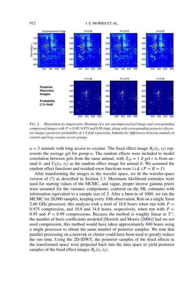
using a Daubechies wavelet with four vanishing moments, periodic boundary con-ditions, and the decomposition completed to J = 6 frequency levels. To investi-gate image compression, we generated a compression plot (Figure 1) as describedin Section 3.5. Note that we were able to preserve a high level of energy whileretaining a small proportion of coefficients. The top panels of Figure 2 containplots of one of the processed 2D gel images (uncompressed and compressed usingP = 0.99,0.975 and 0.95) to demonstrate that the compressed and uncompressedimages look virtually identical. We chose P = 0.975 for our primary analyses,which modeled the T = 646 × 861 = 556,206 pixels using only T ∗

97.5 = 10,634wavelet coefficients, for a compression ratio of more than 50:1. As a sensitivityanalysis, we also ran ISO-FMM with compression levels P = 0.95 and P = 0.99,yielding T ∗

95 = 4958 and T ∗99 = 26,520 coefficients, respectively, which correspond

to compression ratios of over 100:1 and 20:1. We also considered the rectangulartransform, but found this was not as efficient in representing the 2-DE images,with 11,384 coefficients required using P = 0.975, so we chose to use the squaretransform in our analyses.

Let Yi(t1, t2), i = 1, . . . ,53, be the log2-transformed preprocessed gel images.We used the following functional mixed model for these data:

Yi(t1, t2) =3∑

a=1

XiaBa(t1, t2) +21∑

b=1

ZibUb(t1, t2) + Ei(t1, t2),(7)

where Xia = 1 if gel i is from an animal in group a, 0 otherwise, with the groupslabeled as a = 1 control animals, a = 2 animals with short access to cocaine, and


FIG. 2. Illustration of compression: Heatmap of a raw uncompressed gel image and correspondingcompressed images with P = 0.99,0.975 and 0.95 (top), along with corresponding posterior discov-ery images (posterior probability of 1.5-fold expression, bottom) for differences between animals incontrol and long cocaine access groups.

a = 3 animals with long access to cocaine. The fixed effect image Ba(t1, t2) rep-resents the average gel for group a. The random effects were included to modelcorrelation between gels from the same animal, with Zib = 1 if gel i is from an-imal b, and Ub(t1, t2) as the random effect image for animal b. We assumed therandom effect functions and residual error functions were i.i.d. (P = R = I ).

After transforming the images to the wavelet space, we fit the wavelet-spaceversion of (7) as described in Section 3.3. Maximum likelihood estimates wereused for starting values of the MCMC, and vague, proper inverse gamma priorswere assumed for the variance components, centered on the ML estimates withinformation equivalent to a sample size of 2. After a burn-in of 1000, we ran theMCMC for 20,000 samples, keeping every 10th observation. Run on a single Xeon2.66 GHz processor, this analysis took a total of 16.8 hours when run with P =0.975 compression, and 10.8 and 34.8 hours, respectively, when run with P =0.95 and P = 0.99 compressions. Because the method is roughly linear in T ∗,the number of basis coefficients modeled [Herrick and Morris (2006)] had we notused compression, this method would have taken approximately 600 hours usinga single processor to obtain the same number of posterior samples. We note thatparallel processing on a network or cluster could have been used to greatly reducethe run time. Using the 2D-IDWT, the posterior samples of the fixed effects inthe transformed space were projected back into the data space to yield posteriorsamples of the fixed effect images Ba(t1, t2).


Next, we constructed posterior samples for the overall mean gel image,M(t1, t2) = 1/3{B1(t1, t2)+ B2(t1, t2) + B3(t1, t2)}, and to consider contrasts cor-responding to the various between-group comparisons. Here we focus on the im-age corresponding to the difference between the control group and the long co-caine access group, C13(t1, t2) = B1(t1, t2) − B3(t1, t2) (upper right panel of Fig-ure 4). Regions of C13(t1, t2) with large negative values correspond to regions withgreater protein expression for animals given a long access to cocaine. Regionswith large positive values correspond to regions with greater protein expressionfor the control animals. Using the approach described in Section 3.4, we soughtto identify regions of the gel with at least 1.5-fold difference between groups[δ = log2(1.5) = 0.5850], while controlling the FDR at α = 0.10.

Spot-based modeling using Pinnacle. To compare our ISO-FMM image-basedapproach with a standard spot-based method, we applied Pinnacle [Morris, Clarkand Gutstein (2008)] to these data. First, we aligned and preprocessed the images,exactly as described above, to make sure that any difference in results was not dueto preprocessing but due to the spot vs. image-based approach. Applying Pinnacle,we computed the raw mean processed gel, and denoised it using an undecimatedwavelet-based approach. We detected spots based on their pinnacles, defined asany pixel that is a local maxima in both the horizontal and vertical directions ofthe wavelet-denoised average gel whose normalized intensity is greater than the75th percentile on the gel. Using the Pinnacle graphical user interface, we hand-edited the spot detection to remove obvious artifacts, and were left with a totalof 752 detected spots. For each gel, we quantified each spot using the maximalnormalized intensity within a 5 × 5 square around the detected pinnacle, and thenaveraged intensities over replicate gels from the same animal, yielding a 21 × 752matrix containing normalized spot quantifications for each of 752 detected spotsfor the 21 animals. Using this matrix, we performed t-tests for each pinnacle tocompare the samples from animals in the control and long cocaine access groups,and then forwarded the p-values into the fdrtool method [Strimmer (2008)] toobtain the corresponding q-values, or local false discovery rates.

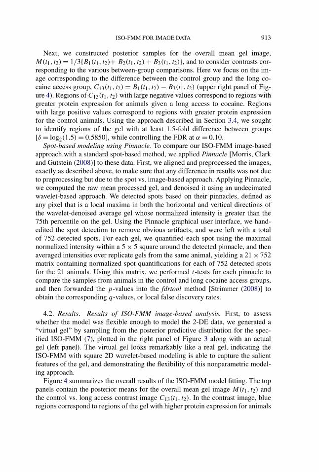
4.2. Results. Results of ISO-FMM image-based analysis. First, to assesswhether the model was flexible enough to model the 2-DE data, we generated a“virtual gel” by sampling from the posterior predictive distribution for the spec-ified ISO-FMM (7), plotted in the right panel of Figure 3 along with an actualgel (left panel). The virtual gel looks remarkably like a real gel, indicating theISO-FMM with square 2D wavelet-based modeling is able to capture the salientfeatures of the gel, and demonstrating the flexibility of this nonparametric model-ing approach.

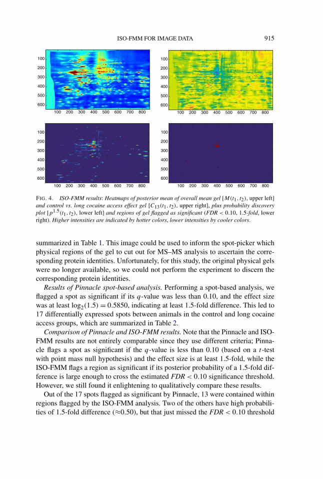
Figure 4 summarizes the overall results of the ISO-FMM model fitting. The toppanels contain the posterior means for the overall mean gel image M(t1, t2) andthe control vs. long access contrast image C13(t1, t2). In the contrast image, blueregions correspond to regions of the gel with higher protein expression for animals


FIG. 3. Virtual Gel Plot of single gel from data example (left panel) and a virtual gel (right panel),found by sampling randomly from the posterior predictive distribution of the ISO-FMM used to fitthe sample data. Note that the ISO-FMM is able to sufficiently capture the structure of real 2D gelsso that the virtual gel looks very much like a real gel that could have come from the example data set.

in the long cocaine access group; red and orange regions indicate higher proteinexpression for control animals; and yellow regions indicate no difference. Notethat we see a mix of blue and red regions, and most of these regions resembleprotein spots. This is what we would expect to see in well-run gel studies withdifferentially expressed protein spots. If most of the effects were all in the samedirection (blue or red), or if the regions were irregular and not spot shaped, thenwe might suspect that the results were driven by some artifacts in the data, forexample, background artifacts, which might indicate a problem in the experiment.

The bottom left panel of Figure 4 is the probability discovery plot, p1.513 (t1, t2),

measuring the posterior probability of at least 1.5-fold expression differences be-tween animals in the control and long cocaine access groups with red regions hav-ing the highest posterior probabilities. The bottom panels of Figure 2 contain thisprobability discovery plot for the different compression levels, and demonstratethat the results are robust to the choice of compression level P . Again, these re-gions of high probability are shaped like protein spots, as we would expect if theywere marking differentially expressed proteins. Applying the FDR < 0.10 crite-rion as described in Section 3.4, we flagged all pixels (t1, t2) with p1.5

13 (t1, t2) >

φ1.50.10 = 0.757 as differentially expressed. These regions are marked in red in the

bottom right panel of Figure 4. There are 27 contiguous regions flagged, which are


FIG. 4. ISO-FMM results: Heatmaps of posterior mean of overall mean gel [M(t1, t2), upper left]and control vs. long cocaine access effect gel [C13(t1, t2), upper right], plus probability discoveryplot [p1.5(t1, t2), lower left] and regions of gel flagged as significant (FDR < 0.10, 1.5-fold, lowerright). Higher intensities are indicated by hotter colors, lower intensities by cooler colors.

summarized in Table 1. This image could be used to inform the spot-picker whichphysical regions of the gel to cut out for MS–MS analysis to ascertain the corre-sponding protein identities. Unfortunately, for this study, the original physical gelswere no longer available, so we could not perform the experiment to discern thecorresponding protein identities.

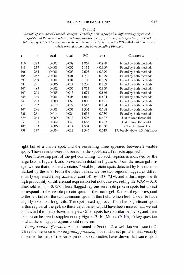
Results of Pinnacle spot-based analysis. Performing a spot-based analysis, weflagged a spot as significant if its q-value was less than 0.10, and the effect sizewas at least log2(1.5) = 0.5850, indicating at least 1.5-fold difference. This led to17 differentially expressed spots between animals in the control and long cocaineaccess groups, which are summarized in Table 2.

Comparison of Pinnacle and ISO-FMM results. Note that the Pinnacle and ISO-FMM results are not entirely comparable since they use different criteria; Pinna-cle flags a spot as significant if the q-value is less than 0.10 (based on a t-testwith point mass null hypothesis) and the effect size is at least 1.5-fold, while theISO-FMM flags a region as significant if its posterior probability of a 1.5-fold dif-ference is large enough to cross the estimated FDR < 0.10 significance threshold.However, we still found it enlightening to qualitatively compare these results.

Out of the 17 spots flagged as significant by Pinnacle, 13 were contained withinregions flagged by the ISO-FMM analysis. Two of the others have high probabili-ties of 1.5-fold difference (≈0.50), but that just missed the FDR < 0.10 threshold


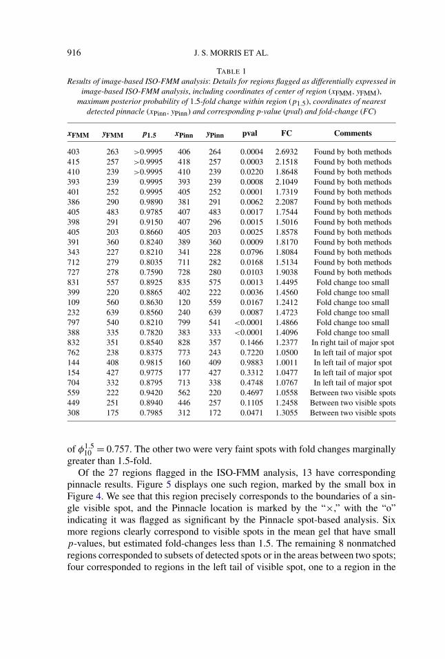
TABLE 1Results of image-based ISO-FMM analysis: Details for regions flagged as differentially expressed in

image-based ISO-FMM analysis, including coordinates of center of region (xFMM, yFMM),maximum posterior probability of 1.5-fold change within region (p1.5), coordinates of nearest

detected pinnacle (xPinn, yPinn) and corresponding p-value (pval) and fold-change (FC)

xFMM yFMM p1.5 xPinn yPinn pval FC Comments

403 263 >0.9995 406 264 0.0004 2.6932 Found by both methods415 257 >0.9995 418 257 0.0003 2.1518 Found by both methods410 239 >0.9995 410 239 0.0220 1.8648 Found by both methods393 239 0.9995 393 239 0.0008 2.1049 Found by both methods401 252 0.9995 405 252 0.0001 1.7319 Found by both methods386 290 0.9890 381 291 0.0062 2.2087 Found by both methods405 483 0.9785 407 483 0.0017 1.7544 Found by both methods398 291 0.9150 407 296 0.0015 1.5016 Found by both methods405 203 0.8660 405 203 0.0025 1.8578 Found by both methods391 360 0.8240 389 360 0.0009 1.8170 Found by both methods343 227 0.8210 341 228 0.0796 1.8084 Found by both methods712 279 0.8035 711 282 0.0168 1.5134 Found by both methods727 278 0.7590 728 280 0.0103 1.9038 Found by both methods831 557 0.8925 835 575 0.0013 1.4495 Fold change too small399 220 0.8865 402 222 0.0036 1.4560 Fold change too small109 560 0.8630 120 559 0.0167 1.2412 Fold change too small232 639 0.8560 240 639 0.0087 1.4723 Fold change too small797 540 0.8210 799 541 <0.0001 1.4866 Fold change too small388 335 0.7820 383 333 <0.0001 1.4096 Fold change too small832 351 0.8540 828 357 0.1466 1.2377 In right tail of major spot762 238 0.8375 773 243 0.7220 1.0500 In left tail of major spot144 408 0.9815 160 409 0.9883 1.0011 In left tail of major spot154 427 0.9775 177 427 0.3312 1.0477 In left tail of major spot704 332 0.8795 713 338 0.4748 1.0767 In left tail of major spot559 222 0.9420 562 220 0.4697 1.0558 Between two visible spots449 251 0.8940 446 257 0.1105 1.2458 Between two visible spots308 175 0.7985 312 172 0.0471 1.3055 Between two visible spots

of φ1.510 = 0.757. The other two were very faint spots with fold changes marginally

greater than 1.5-fold.Of the 27 regions flagged in the ISO-FMM analysis, 13 have corresponding

pinnacle results. Figure 5 displays one such region, marked by the small box inFigure 4. We see that this region precisely corresponds to the boundaries of a sin-gle visible spot, and the Pinnacle location is marked by the “×,” with the “o”indicating it was flagged as significant by the Pinnacle spot-based analysis. Sixmore regions clearly correspond to visible spots in the mean gel that have smallp-values, but estimated fold-changes less than 1.5. The remaining 8 nonmatchedregions corresponded to subsets of detected spots or in the areas between two spots;four corresponded to regions in the left tail of visible spot, one to a region in the


TABLE 2Results of spot-based Pinnacle analysis: Details for spots flagged as differentially expressed in

spot-based Pinnacle analysis, including location (x, y), p-value (pval), q-value (qval) andfold-change (FC). Also included is the maximum p1.5(t1, t2) from the ISO-FMM within a 5-by-5

neighborhood around the corresponding Pinnacle

x y pval qval FC p1.5 Comments

410 239 0.002 0.008 1.865 >0.999 Found by both methods418 257 <0.001 0.002 2.152 >0.999 Found by both methods406 264 <0.001 0.003 2.693 >0.999 Found by both methods405 252 <0.001 0.001 1.732 0.999 Found by both methods393 239 0.001 0.004 2.105 0.999 Found by both methods381 291 0.006 0.014 2.209 0.989 Found by both methods407 483 0.002 0.007 1.754 0.979 Found by both methods407 203 0.005 0.013 1.671 0.866 Found by both methods389 360 0.001 0.005 1.817 0.824 Found by both methods341 228 0.080 0.068 1.808 0.821 Found by both methods711 282 0.017 0.027 1.513 0.804 Found by both methods407 296 0.001 0.007 1.502 0.788 Found by both methods728 281 0.014 0.024 1.638 0.759 Found by both methods379 263 0.009 0.018 1.595 0.487 Just missed threshold257 60 0.062 0.048 1.663 0.463 Just missed threshold409 163 0.006 0.014 1.504 0.160 FC barely above 1.5798 177 0.004 0.012 1.543 0.019 FC barely above 1.5, faint spot

right tail of a visible spot, and the remaining three appeared between 2 visiblespots. These results were not found by the spot-based Pinnacle approach.

One interesting part of the gel containing two such regions is indicated by thelarge box in Figure 4, and presented in detail in Figure 6. From the mean gel im-age, we see that this field contains 7 visible protein spots detected by Pinnacle, asmarked by the ×’s. From the other panels, we see two regions flagged as differ-entially expressed (long access > control) by ISO-FMM, and a third region withhigh probability of differential expression but not quite exceeding the FDR = 0.10threshold φ1.5

0.10 = 0.757. These flagged regions resemble protein spots but do notcorrespond to the visible protein spots in the mean gel. Rather, they correspondto the left tails of the two dominant spots in this field, which both appear to haveslightly extended long tails. The spot-based approach found no significant spotsin this region of the gel, so these discoveries would have been missed had we notconducted the image-based analysis. Other spots have similar behavior, and theirdetails can be seen in supplementary Figures 3–10 [Morris (2010)]. A key questionis what these flagged regions could represent.

Interpretation of results. As mentioned in Section 2, a well-known issue in 2-DE is the presence of co-migrating proteins, that is, distinct proteins that visuallyappear to be part of the same protein spot. Studies have shown that some spots


FIG. 5. Specific Results 1: Posterior mean of overall mean gel (upper left), effect gel (upper right),probability discovery plot (lower left), and indicating ISO-FMM flagged regions (lower right) forregion marked by small box in Figure 4, with pinnacles for detected spots marked (×), and differentialexpression in Pinnacle analysis indicated by a (o). Note that region flagged by ISO-FMM correspondsto visible spot also detected by Pinnacle analysis.

FIG. 6. Specific Results 2: Posterior mean of overall mean gel (upper left), effect gel (upper right),probability discovery plot (lower left), and indicating ISO-FMM flagged regions (lower right) forregion marked by large box in Figure 4, with pinnacles for detected spots marked (×), and differentialexpression in Pinnacle analysis indicated by a (o). Note that regions flagged by ISO-FMM correspondto tails of visible spots that themselves are not differentially expressed. These results are not foundby the Pinnacle analysis.


on a gel can have as many as 5 or 6 distinct proteins [Gygi et al. (2000)]. Theseco-migrating proteins can be different proteins or post-translational modificationsof the same protein, which can also be functionally distinct. If two proteins havesimilar combinations of pH and molecular mass, it is possible that the proteinswill run together in the same visible spot on the 2-DE. It can be very difficult, andsometimes impossible, for any spot detection method to deconvolve these multiplespots into separate protein spots, especially if one of them has considerably higherabundance than the others. The inability to resolve these co-migrating proteins isone of the key criticisms levied against 2-DE. The significant regions flagged byISO-FMM but not by Pinnacle which appear in the tail of a visible spot or betweentwo visible spots may indicate differentially expressed co-migrating proteins visi-bly masked by a more abundant non differentially-expressed protein, and that theseproteins were completely missed by the spot-based analysis. Studies are underwayto confirm this possibility.

In this way, the image-based modeling approach may be able to extract moreprotein information from the gels than spot-based approaches. Because spot-basedmodeling approaches have been almost universally used to date, this means thatperhaps 2-DE contains more proteomic information than was previously known.The image-based approach may effectively increase the realized resolution of thegels and better extract the proteomic information they contain. Further biologicalstudies are needed to validate these conjectures.

5. Discussion. In this paper we have discussed a general Bayesian methodfor quantitative image data based on functional mixed models that uses an isomor-phic modeling approach. The underlying FMM framework is very general, cansimultaneously model any number of covariates, each having their own fixed ef-fect image of general form, and can account for correlation between the imagesusing random effect images and between-image covariance matrices. The resultsfrom the method can be used to perform FDR-based Bayesian inference that takesboth practical and statistical significance into account, and flags significant regionsof the fixed effect images.

Previous work on functional mixed models has been limited to single-dimen-sional functions; here we have shown how this approach can be applied to imagesof dimension 2 or higher. Also, previous work on functional mixed models hasbeen based on specific modeling strategies using smoothing splines [Guo (2002)]or wavelets [Morris and Carroll (2006)]. In this paper we have described a gen-eral modeling strategy that involves using an isomorphic transformation to mapthe data to an alternative space, where modeling can be done more parsimoniouslyand smoothing or regularization naturally done, and results can be mapped backto the original data space for final inference. This method, ISO-FMM, containsWFMM as a special case, but can be also applied much more generally using otherisomorphic transformations. With each proposed transformation, careful thoughtneeds to be given to the modeling choices and their implications in the data space,


and thus further work is required to apply this approach using certain other trans-formations. This general modeling strategy can be used for the 1D FMM, or forthe higher dimensional FMM that is the primary interest of this paper. This iso-morphic modeling approach is a general strategy with potential for application toa variety of other contexts.

We introduced a compression method to reduce the dimensionality of the datathat is appropriate when the chosen isomorphic transformation leads to a sparserepresentation for all of the images, as is true for wavelets. This compressionmethod can also be applied to any functional data, 1-D or higher. We have found itis possible to use compression to speed up the computations by one or two ordersof magnitude, which greatly reduces the memory overhead requirements withoutsubstantively changing the results.

While the method is complex, we have developed general freely availablesoftware (http://biostatistics.mdanderson.org/SoftwareDownload/SingleSoftware.aspx?Software_Id=70) to implement it that is efficient enough to handle very largedata sets and complex models, and is relatively straightforward to use, consideringthe complexity of the method. If the user is satisfied with automatic vague properpriors and default wavelet bases, then the method can run completely automati-cally if the user simply specifies the Y,X and Z matrices. Users who wish to usealternative basis functions can compute the D matrix themselves and feed that intothe program, indicating which groups of coefficients will share common smooth-ing parameters. The code automatically generates posterior means and quantiles(default 0.005, 0.01, 0.025, 0.975, 0.99, 0.995) for prespecified contrasts involvingthe Ba(t1, t2), plus the posterior probabilities of specific effect sizes pδ

a(t1, t2) forspecified choices of δ {default δ = log2(1.25), log2(1.5), log2(2.0)}. Thus, plotslike those generated in Figure 4 can be quickly generated once the method is run.The code is continually being updated as the scope of the FMM framework is ex-tended, so more features will be added in the future, as will an R interface forrunning the method.

Applying this method to 2-DE data, we found that the ISO-FMM was able tofind differentially expressed proteins that may be co-migrating proteins that wouldnot have been found using the usual spot-based analysis approaches. The ISO-FMM may be capable of extracting more proteomic information from the gels thanwas previously known to be there. This method can easily be applied to DIGE databy just modeling Yi(t1, t2) to be the log ratio of the two channels. Although thispaper focused on 2-DE, the ISO-FMM can be applied to any type of quantitativeimage data, including fMRI, LC–MS and other commonly encountered applica-tions. This rigorous, automated method can be useful in extracting informationand performing inference for quantitative image data.

Acknowledgments. We thank Andrew Dowsey and Brittan Clark for aligningthe gels, and George Koob from Scripps Research Institute for helpful advice. Wealso thank Lee Ann Chastain for excellent editorial assistance.

http://biostatistics.mdanderson.org/SoftwareDownload/SingleSoftware.aspx?Software_Id=70

http://biostatistics.mdanderson.org/SoftwareDownload/SingleSoftware.aspx?Software_Id=70


SUPPLEMENTARY MATERIAL

Supplement A: Computational details for wavelet-space implementation ofISO-FMM for image data (DOI: 10.1214/10-AOAS407SUPPA). Computationaldetails for wavelet implementation of the ISO-FMM for image data, includingempirical Bayes method for estimating regularization parameters, MCMC detailsand Metropolis–Hastings details for covariance parameters.

Supplement B: Supplementary figures (DOI: 10.1214/10-AOAS407SUPPB).Supplementary figures, including a virtual 2d gel simulated from the model,a demonstration of the spatial covariance structure induced by the model and 8plots containing zoomed-in results from analysis of application data in certain in-teresting regions of the gel.

Supplement C: Spatial covariance structure in image WFMM (DOI:10.1214/10-AOAS407SUPPC). Basic illustration of spatial covariance structureinduced by ISO-FMM with 2D wavelet transforms and independence assumed inthe wavelet space. Basic demonstration described, and some plots provided. Moviefile spatial_covariance.wvm also available as supplementary material to further il-lustrate these results.

Supplement D: Movie file illustrating spatial covariance structure of ISO-WFMM with 2D wavelet transform (DOI: 10.1214/10-AOAS407SUPPD). Win-dows movie file illustrating the nonstationary spatial covariance structure inducedby the ISO-FMM with 2D wavelet bases, with independence assumed amongwavelet coefficients. Description of data yielding this movie is provided in thefile “Spatial Covariance Structure in Image WFMM.pdf,” also available as supple-mentary material.

REFERENCES

AHMED, S. H. and KOOB, G. F. (1998). Transition from moderate to excessive drug intake: Changein hedonic set point. Science 282 298–300.

BENJAMINI, Y. and HOCHBERG, Y. (1995). Controlling the false discovery rate: A practical andpowerful approach to multiple testing. J. Roy. Statist. Soc. Ser. B 57 289–300. MR1325392

CANDES, E. J. and DONOHO, D. L. (2000). Curvelets, multiresolution representation, and scalinglaws. In SPIE Wavelet Applications in Signal and Image Processing VIII (A. Aldroubi, A. F. Laineand M. A. Unser, eds.). Proc. SPIE 4119. Hindawi, New York.

CLARK, B. N. and GUTSTEIN, H. B. (2008). The myth of automated, high-throughput two-dimensional gel electrophoresis. Proteomics 8 1197–1203.

CLYDE, M., PARMIGIANI, G. and VIDAKOVIC, B. (1998). Multiple shrinkage and subset selectionin wavelets. Biometrika 85 391–401. MR1649120

DAWID, A. P. (1981). Some matrix-variate distribution theory: Notational considerations and aBayesian application. Biometrika 68 265–274. MR0614963

DIGGLE, P. J. and AL WASEL, I. (1997). Spectral analysis of replicated biomedical time series.J. Roy. Statist. Soc. Ser. C 46 31–71. MR1452286

DO, M. N. and VETTERLI, M. (2001). Beyond Wavelets (J. Stoeckler and G. V. Welland, eds.).Academic Press, New York. MR2136835

http://dx.doi.org/10.1214/10-AOAS407SUPPA

http://dx.doi.org/10.1214/10-AOAS407SUPPB

http://dx.doi.org/10.1214/10-AOAS407SUPPC

http://dx.doi.org/10.1214/10-AOAS407SUPPD

http://www.ams.org/mathscinet-getitem?mr=1325392






DO, M. N. and VETTERLI, M. (2005). The contourlet transform: An efficient directional multireso-lution image representation. IEEE Trans. Image Process. 14 2091–2106.

DOWSEY, A. W., DUNN, M. J. and YANG, G. Z. (2008). Automated image alignment for 2D gelelectrophoresis in a high-throughput proteomics pipeline. Bioinformatics 24 950–957.

FAERGESTAD, E. M., RYE, M., WALCZAK, B., GIDSKEHAUG, L., WOLD, J. P., GROVE, H.,JIA, X., HOLLUNG, K., INDAHL, U. G., WESTAD, F., VAN DEN BERG, F. and MARTENS,H. (2007). Pixel-based analysis of multiple images for the indentification of changes: A novelapproach applied to unravel patterns of 2-D electrophoresis gel images. Proteomics 7 3450–3461.

FEILNER, M., VAN DE VILLE, D. and UNSER, M. (2005). An orthogonal family of quin-cunx wavelets with continuously adjustable order. IEEE Trans. Signal Process. 14 499–510.MR2128291

GYGI, S. P., CORTHALS, G. L., ZHANG, Y., ROCHON, Y. and AEBERSOLD, R. (2000). Evaluationof two-dimensional gel electrophoresis-based proteome analysis technology. Proc. Natl. Acad.Sci. USA 97 9390–9395.

GUO, W. (2002). Functional mixed effects models. Biometrics 58 121–128. MR1891050HEINRICHS, S. C., MENZAGHI, F., SCHULTEIS, G., KOOB, G. F. and STINUS, L. (1995). Sup-

pression of corticotropin-releasing factor in the amygdala attenuates aversive consequences ofmorphine withdrawal. Behavioral Pharmacology 6 74–80.

HERRICK, R. C. and MORRIS, J. S. (2006). Wavelet-based functional mixed model analysis: Com-putational considerations. In Proceedings, Joint Statistical Meetings, ASA Section on StatisticalComputing 2051–2053. Amer. Statist. Assoc., Alexandria, VA.

KARP, N. A. and LILLEY, K. S. (2005). Maximizing sensitivity for detecting changes in proteinexpression: Experimental design using minimal CyDyes. Proteomics 5 3105–3115.

KOKKINIDIS, L., ZACHARKO, R. M. and PREDY, P. A. (1980). Post-amphetamine depression ofself-stimulation responding from the substantia nigra: Reversal by tricyclic antidepressants. Phar-macol Biochem. Behav. 12 379–383.

LEITH, N. J. and BARRETT, R. J. (1976). Amphetamine and the reward system: Evidence for toler-ance and post-drug depression. Psychopharmacologia 46 19–25.

LILLEY, K. S. (2003). Protein profiling using two-dimensional difference gel electrophoresis (2-DDIGE). In Current Protocols in Protein Science, Chapter 22, Unit 22.2. Wiley, New York.

MALLAT, S. G. (1989). A theory for multiresolution signal decomposition: The wavelet representa-tion. IEEE Trans. Pattern Anal. Mach. Intell. 11 674–693.

MARKOU, A. and KOOB, G. (1992). Bromocriptine reverses the elevation in intracranial self-stimulation thresholds observed in a rat model of cocaine withdrawal. Neuropsychopharmacology7 213–224.

MORRIS, J. S. (2010). Supplement to “Automated analysis of quantitative image data using iso-morphic functional mixed models, with application to proteomics data.” DOI: 10.1214/10-AOAS407SUPPA, DOI: 10.1214/10-AOAS407SUPPB, DOI: 10.1214/10-AOAS407SUPPC,DOI: 10.1214/10-AOAS407SUPPD.

MORRIS, J. S., ARROYO, C., COULL, B., RYAN, L. M., HERRICK, R. and GORTMAKER, S. L.(2006). Using wavelet-based functional mixed models to characterize population heterogeneityin accelerometer profiles: A case study. J. Amer. Statist. Assoc. 101 1352–1364. MR2307570

MORRIS, J. S., BROWN, P. J., HERRICK, R. C., BAGGERLY, K. A. and COOMBES, K. R. (2008).Bayesian analysis of mass spectrometry data using wavelet-based functional mixed models. Bio-metrics 12 479–489. MR2432418

MORRIS, J. S. and CARROLL, R. J. (2006). Wavelet-based functional mixed models. J. Roy. Statist.Soc. Ser. B 68 179–199. MR2188981

MORRIS, J. S., CLARK, B. N. and GUTSTEIN, H. B. (2008). Pinnacle: A fast, automatic and accu-rate method for detecting and quantifying protein spots in 2-dimensional gel electrophoresis data.Bioinformatics 24 529–536.




http://dx.doi.org/10.1214/10-AOAS407SUPPB

http://dx.doi.org/10.1214/10-AOAS407SUPPC

http://dx.doi.org/10.1214/10-AOAS407SUPPD






MORRIS, J. S., VANNUCCI, M., BROWN, P. J. and CARROLL, R. J. (2003). Wavelet-based non-parametric modeling of hierarchical functions in colon carcinogenesis. J. Amer. Statist. Assoc. 98573–583.

MORRIS, J. S., CLARK, B. N., WEI, W. and GUTSTEIN, H. B. (2010). Evaluting the performanceof new approaches to spot quantification and differential expression in 2-dimensional gel elec-trophoresis studies. Journal of Proteome Research 9 595–604.

MUELLER, P., PARMIGIANI, G., ROBERT, C. and ROUSSEAU, J. (2004). Optimal sample size formultiple testing: The case of gene expression microarrays. J. Amer. Statist. Assoc. 99 990–1001.MR2109489

PARSONS, L. H., KOOB, G. F. and WEISS, F. (1995). Serotonin dysfunction in the nucleus accum-bens of rats during withdrawal after unlimited access to intravenous cocaine. Journal of Pharma-cology and Experimental Therapeutics 274 1182–1191.

RAMSAY, J. O. and SILVERMAN, B. W. (1997). Functional Data Analysis. Springer, New York.MR2168993

REISS, P. T. and OGDEN, R. T. (2009). Functional generalized linear models with images as pre-dictors. Biometrics. Published online May 8, 2009.

RICHTER, R. and WEISS, F. (1999). In vivo CRF release in rat amygdala is increased during cocainewithdrawal in self-administering rats. Synapse 32 254–261.

SAMPSON, P. D. and GUTTORP, P. (1992). Nonparametric estimation of nonstationary spatial co-variance structure. J. Amer. Statist. Assoc. 87 108–119.

SCHULTEIS, G., MARKOU, A., GOLD, L. H., STINUS, L. and KOOB, G. F. (1994). Relative sensi-tivity to naloxone of multiple indices of opiate withdrawal: A quantitative dose–response analysis.Journal of Pharmacology and Experimental Therapeutics 271 1391–1398.

SMITH, M. and FAHRMEIR, L. (2007). Spatial Bayesian variable selection with application to func-tional magnetic resonance imaging. J. Amer. Statist. Assoc. 102 417–431. MR2370843

STOREY, J. D. (2003). The positive false discovery rate: A Bayesian interpretation and the q-value.Ann. Statist. 31 2013–2035. MR2036398

STRIMMER, K. (2008). fdrtool: A versitile R package for estimating local and tail area-based falsediscovery rates. Bioinformatics 24 1461–1462.

WEISS, F., MARKOU, A., LORANG, M. T. and KOOB, G. F. (1992). Basal extracellular dopaminelevels in the nucleus accumbens are decreased during cocaine withdrawal after unlimited-accessself-ad ministration. Brain Research 593 314–318.

J. S. MORRIS

V. BALADANDAYUTHAPANI

R. C. HERRICK

H. GUTSTEIN

UNIVERSITY OF TEXAS

MD ANDERSON CANCER CENTER

UNIT 1411, PO BOX 301402HOUSTON, TEXAS 77230-1402USAE-MAIL: [email protected]

[email protected]@[email protected]

URL: http://works.bepress.com/jeffrey_s_morris

P. SANNA

SCRIPPS RESEARCH INSTITUTE

LA JOLLA, CALIFORNIA

USAE-MAIL: psanna@scripps





mailto:[email protected]




http://works.bepress.com/jeffrey_s_morris

mailto:psanna@scripps

Automated analysis of quantitative image data using ... · from any application, ... In 2D gel...

Documents

Transcript of Automated analysis of quantitative image data using ... · from any application, ... In 2D gel...