
Autodock by Anop Singh Ranawat
22
Transcript of Autodock by Anop Singh Ranawat
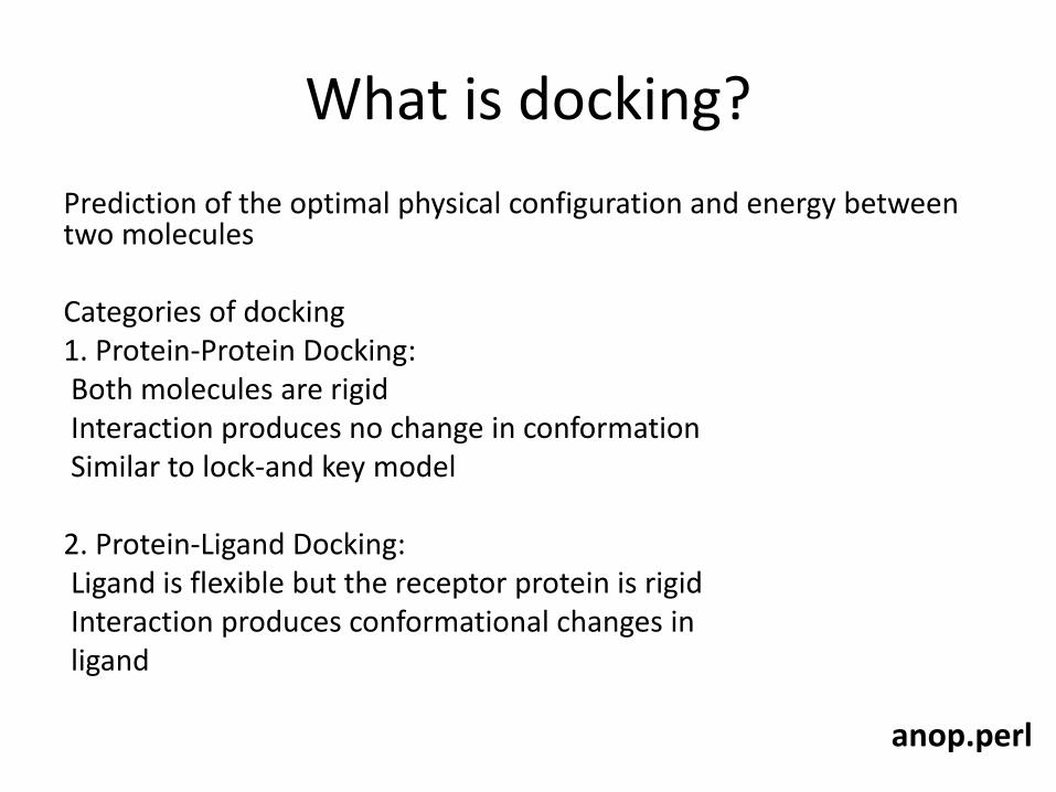
What is docking?
Prediction of the optimal physical configuration and energy between two molecules Categories of docking 1. Protein-Protein Docking: Both molecules are rigid Interaction produces no change in conformation Similar to lock-and key model 2. Protein-Ligand Docking: Ligand is flexible but the receptor protein is rigid Interaction produces conformational changes in ligand
anop.perl
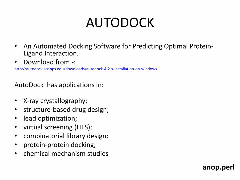
AUTODOCK
• An Automated Docking Software for Predicting Optimal Protein-Ligand Interaction.
• Download from -: http://autodock.scripps.edu/downloads/autodock-4-2-x-installation-on-windows
AutoDock has applications in: • X-ray crystallography; • structure-based drug design; • lead optimization; • virtual screening (HTS); • combinatorial library design; • protein-protein docking; • chemical mechanism studies
anop.perl
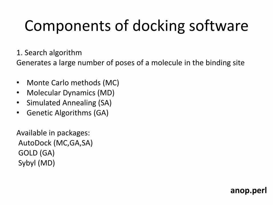
Components of docking software
1. Search algorithm Generates a large number of poses of a molecule in the binding site
• Monte Carlo methods (MC) • Molecular Dynamics (MD) • Simulated Annealing (SA) • Genetic Algorithms (GA)
Available in packages: AutoDock (MC,GA,SA) GOLD (GA) Sybyl (MD)
anop.perl
Components of docking software
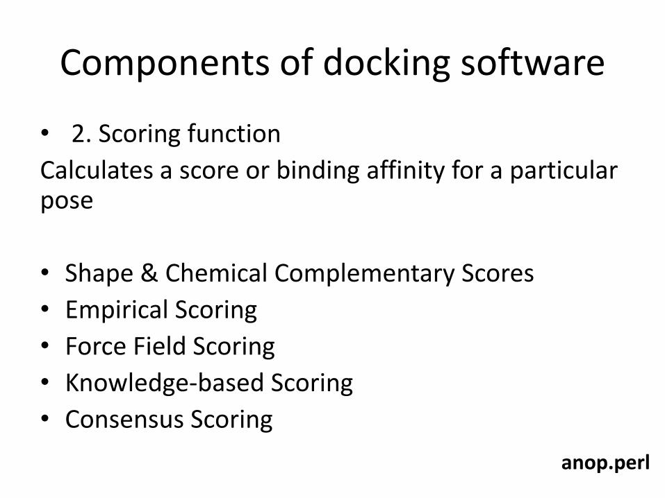
• 2. Scoring function
Calculates a score or binding affinity for a particular pose
• Shape & Chemical Complementary Scores
• Empirical Scoring
• Force Field Scoring
• Knowledge-based Scoring
• Consensus Scoring
anop.perl
The Algorithms
anop.perl

Simulated Annealing
• Algorithm modeled after the cooling of a solution to form glass, though it’s better explained by crystal formation
• Given a long enough cooling time, molecules will relax into their lowest energy state to form the largest crystals
– Quick cooling - highly disordered system
– Slow cooling - highly ordered crystal, with each molecule in its lowest energy state
– Algorithm simulates either linear or proportional slow cooling
anop.perl
The SA Algorithm
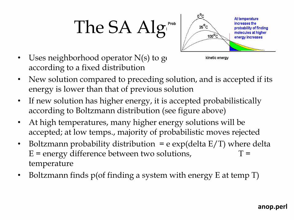
• Uses neighborhood operator N(s) to generate a set of solutions according to a fixed distribution
• New solution compared to preceding solution, and is accepted if its energy is lower than that of previous solution
• If new solution has higher energy, it is accepted probabilistically according to Boltzmann distribution (see figure above)
• At high temperatures, many higher energy solutions will be accepted; at low temps., majority of probabilistic moves rejected
• Boltzmann probability distribution = e exp(delta E/T) where delta E = energy difference between two solutions, T = temperature
• Boltzmann finds p(of finding a system with energy E at temp T)
anop.perl
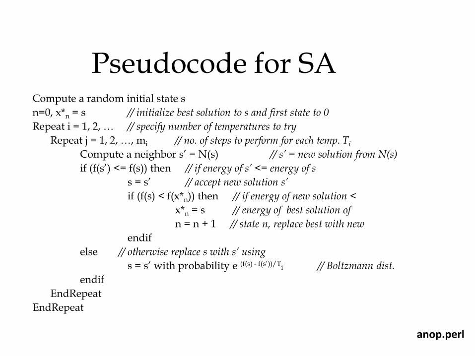
Pseudocode for SA Compute a random initial state s
n=0, x*n = s // initialize best solution to s and first state to 0
Repeat i = 1, 2, … // specify number of temperatures to try
Repeat j = 1, 2, …, mi // no. of steps to perform for each temp. Ti
Compute a neighbor s’ = N(s) // s’ = new solution from N(s)
if (f(s’) <= f(s)) then // if energy of s’ <= energy of s
s = s’ // accept new solution s’
if (f(s) < f(x*n)) then // if energy of new solution <
x*n = s // energy of best solution of
n = n + 1 // state n, replace best with new
endif
else // otherwise replace s with s’ using
s = s’ with probability e (f(s) - f(s’))/Ti // Boltzmann dist.
endif
EndRepeat
EndRepeat
anop.perl
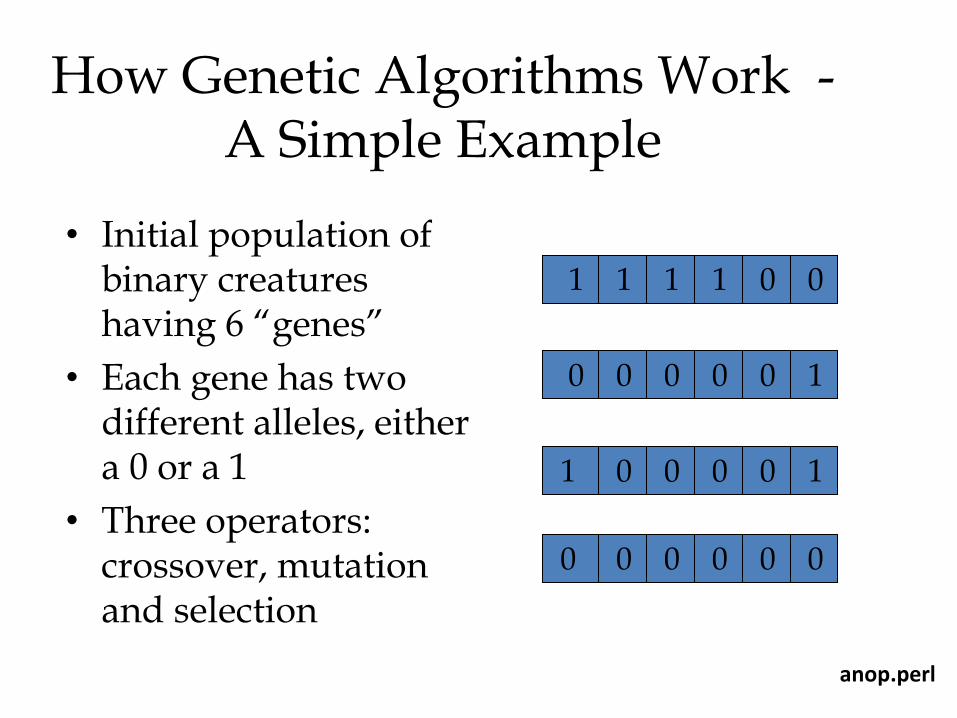
How Genetic Algorithms Work - A Simple Example
• Initial population of binary creatures having 6 “genes”
• Each gene has two different alleles, either a 0 or a 1
• Three operators: crossover, mutation and selection
1 1 1 1 0 0
0 0 0 0 0 1
1 0 0 0 0 1
0 0 0 0 0 0
anop.perl
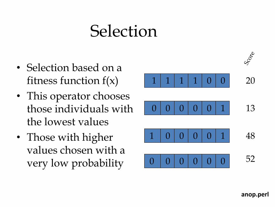
Selection
• Selection based on a fitness function f(x)
• This operator chooses those individuals with the lowest values
• Those with higher values chosen with a very low probability
1 1 1 1 0 0
0 0 0 0 0 1
1 0 0 0 0 1
0 0 0 0 0 0
20
13
48
52
anop.perl
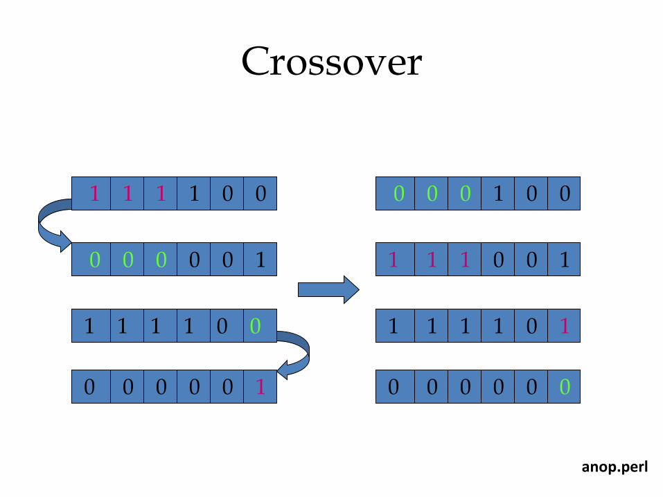
Crossover
0 0 0 1 0 0
1 1 1 0 0 1
1 1 1 1 0 1
0 0 0 0 0 0
1 1 1 1 0 0
0 0 0 0 0 1
1 1 1 1 0 0
0 0 0 0 0 1
anop.perl

Mutation
0 0 1 1 0 0
1 1 1 0 1 1
1 1 1 1 0 1
0 0 1 0 1 0
0 0 0 1 0 0
1 1 1 0 0 1
1 1 1 1 0 1
0 0 0 0 0 0
anop.perl

Replacement
• Lower scoring individuals create more offspring, higher scoring ones create fewer or none at all
• Offspring replace parental generation
• “Elitism” function allows best individual from parent generation to persist, if it is a better solution than new individuals created
• Cycle of selection, mutation, crossover and replacement
repeated
0 0 1 1 0 0
1 1 1 0 1 1
1 1 1 1 0 1
0 0 1 0 1 0
15 1
9 1
22 0
1 2
anop.perl
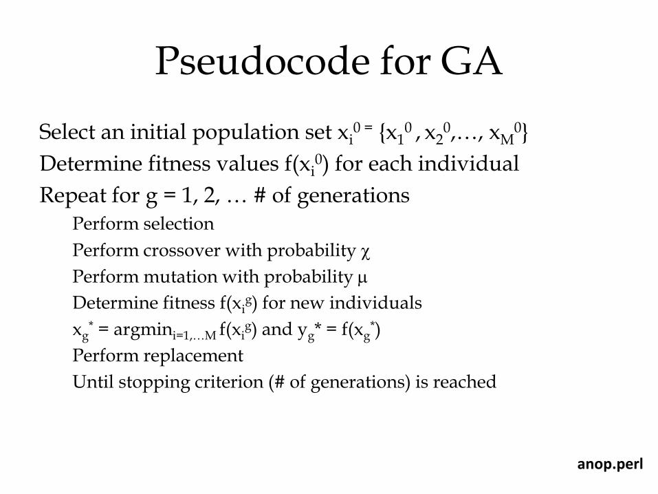
Pseudocode for GA
Select an initial population set xi0 = {x1
0 , x20,…, xM
0}
Determine fitness values f(xi0) for each individual
Repeat for g = 1, 2, … # of generations Perform selection
Perform crossover with probability
Perform mutation with probability
Determine fitness f(xig) for new individuals
xg* = argmini=1,…M f(xi
g) and yg* = f(xg*)
Perform replacement
Until stopping criterion (# of generations) is reached
anop.perl

How GA works in AutoDock
• Ligand’s “genes” are its x, y and z coordinates
• These form a unit vector, which is given a random rotation angle between 0
o
and 360o
to form a quaternion
• Additional genes may represent torsion angles between bonds of the ligand
anop.perl
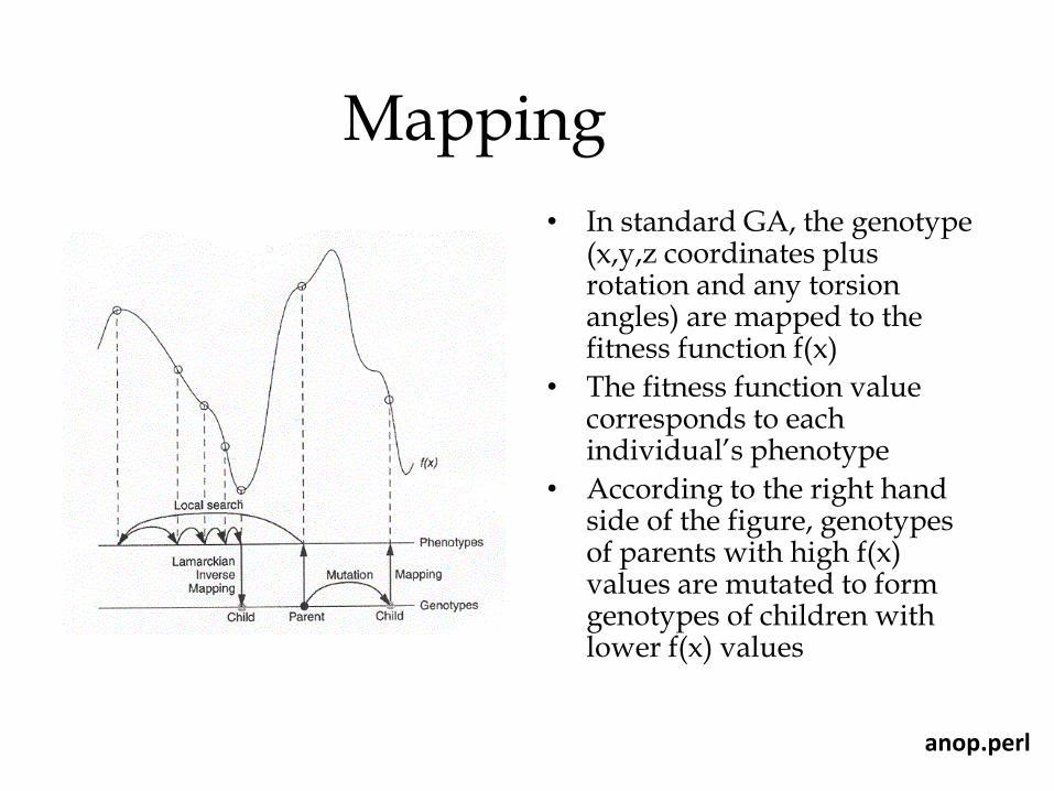
Mapping
• In standard GA, the genotype (x,y,z coordinates plus rotation and any torsion angles) are mapped to the fitness function f(x)
• The fitness function value corresponds to each individual’s phenotype
• According to the right hand side of the figure, genotypes of parents with high f(x) values are mutated to form genotypes of children with lower f(x) values
anop.perl
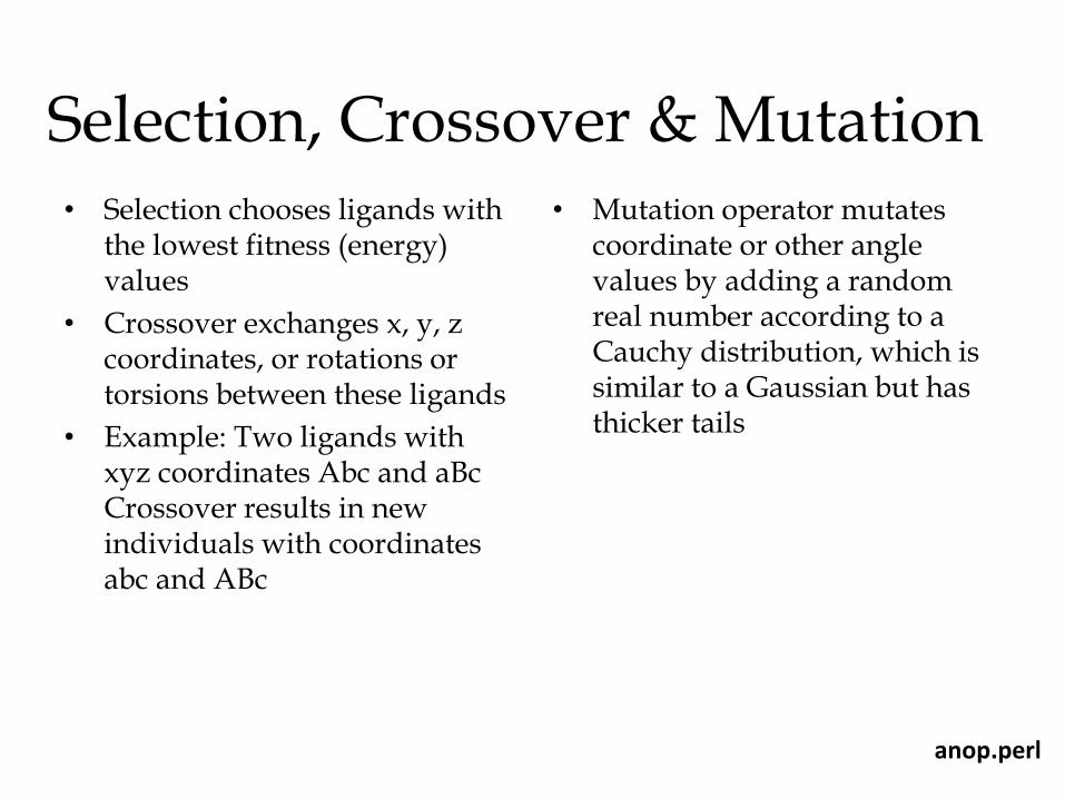
Selection, Crossover & Mutation • Selection chooses ligands with
the lowest fitness (energy) values
• Crossover exchanges x, y, z coordinates, or rotations or torsions between these ligands
• Example: Two ligands with xyz coordinates Abc and aBc Crossover results in new individuals with coordinates abc and ABc
• Mutation operator mutates coordinate or other angle values by adding a random real number according to a Cauchy distribution, which is similar to a Gaussian but has thicker tails
anop.perl
Replacement
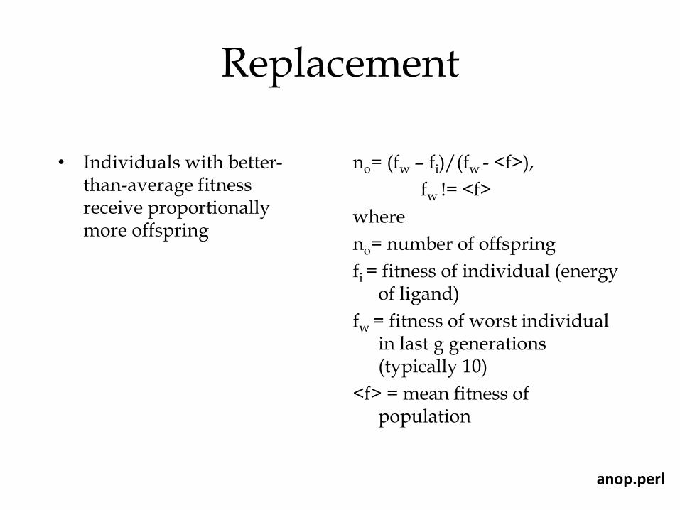
• Individuals with better-than-average fitness receive proportionally more offspring
no= (fw – fi)/(fw - <f>),
fw != <f>
where
no= number of offspring
fi = fitness of individual (energy of ligand)
fw = fitness of worst individual in last g generations (typically 10)
<f> = mean fitness of population
anop.perl
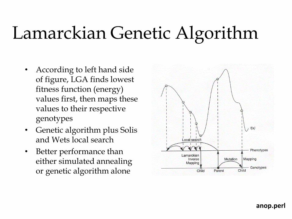
Lamarckian Genetic Algorithm
• According to left hand side of figure, LGA finds lowest fitness function (energy) values first, then maps these values to their respective genotypes
• Genetic algorithm plus Solis and Wets local search
• Better performance than either simulated annealing or genetic algorithm alone
anop.perl
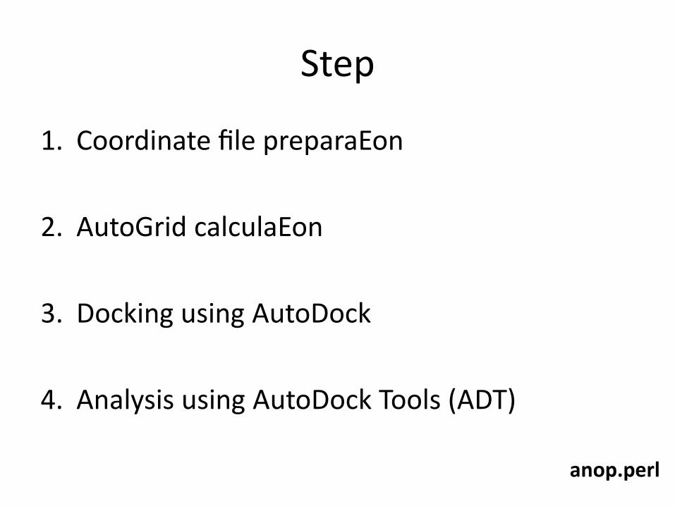
Step
1. Coordinate file preparaEon
2. AutoGrid calculaEon
3. Docking using AutoDock
4. Analysis using AutoDock Tools (ADT)
anop.perl

• Get detail
autodock.scripps.edu/faqs.../autodock4.../AutoDock4.2_UserGuide.pdf
anop.perl