Asymptotically Efficient Estimation of Models Defined by ... - UCLA Econ · Asymptotically...
74
Asymptotically Efficient Estimation of Models Defined by Convex Moment Inequalities Hiroaki Kaido Andres Santos Boston University UC San Diego Andres Santos UCSD
-
Upload
dinhnguyet -
Category
Documents
-
view
223 -
download
0
Transcript of Asymptotically Efficient Estimation of Models Defined by ... - UCLA Econ · Asymptotically...

Asymptotically Efficient Estimation of ModelsDefined by Convex Moment Inequalities
Hiroaki Kaido Andres Santos
Boston University UC San Diego
Andres Santos UCSD

The Model
Consider X ∼ P0 with X ∈ X ⊆ RdX , θ ∈ Θ ⊂ Rdθ and restriction:
F (
∫m(x, θ)dP0(x)) ≤ 0
where m : X ×Θ→ Rdm and F : Rdm → RdF are known functions.
Under Identification• Semiparametric efficiency bound may exist.• Possible to construct efficient estimator.
Partial Identification• What does semiparametric efficiency bound mean?• Is there an efficient estimator?
Andres Santos UCSD
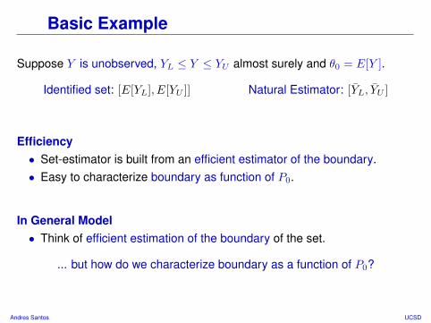
Basic Example
Suppose Y is unobserved, YL ≤ Y ≤ YU almost surely and θ0 = E[Y ].
Identified set: [E[YL], E[YU ]] Natural Estimator: [YL, YU ]
Efficiency• Set-estimator is built from an efficient estimator of the boundary.• Easy to characterize boundary as function of P0.
In General Model• Think of efficient estimation of the boundary of the set.
... but how do we characterize boundary as a function of P0?
Andres Santos UCSD
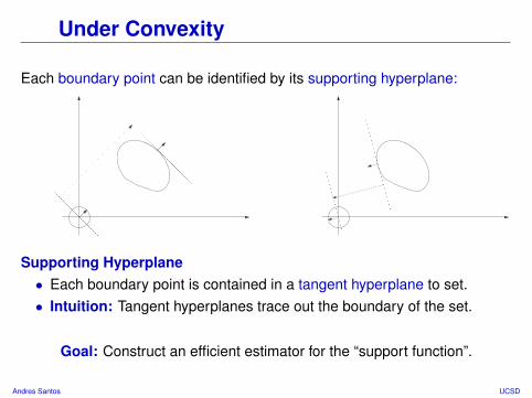
Under Convexity
Each boundary point can be identified by its supporting hyperplane:
Supporting Hyperplane• Each boundary point is contained in a tangent hyperplane to set.• Intuition: Tangent hyperplanes trace out the boundary of the set.
Goal: Construct an efficient estimator for the “support function”.
Andres Santos UCSD
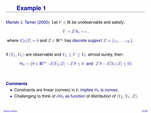
Example 1
Manski & Tamer (2002): Let Y ∈ R be unobservable and satisfy:
Y = Z ′θ0 + ε ,
where E[ε|Z] = 0 and Z ∈ Rdθ has discrete support Z ≡ z1, . . . zK.
If (YL, YU ) are observable and YL ≤ Y ≤ YU almost surely, then:
Θ0 = θ ∈ Rdθ : E[YL|Z]− Z ′θ ≤ 0 and Z ′θ − E[YU |Z] ≤ 0
Comments• Constraints are linear (convex) in θ, implies Θ0 is convex.• Challenging to think of ∂Θ0 as function of distribution of (YL, YU , Z).
Andres Santos UCSD

Example 1
Θ0 = θ ∈ Rdθ : E[YL|Z]− Z ′θ ≤ 0 and Z ′θ − E[YU |Z] ≤ 0
Role of mL: Let x ≡ (yL, yU , z), use mL(x) to pick moments we need.∫mL(x)dP0(x) =
(E[YL1Z = z1], . . . , E[YL1Z = zK])′(E[YU1Z = z1], . . . , E[YU1Z = zK])′
(P (Z = z1), . . . , P (Z = zK))′
Role of FL: Use FL function to construct expressions we require:
FL(
∫mL(x)dP0(x)) =
(−(E[YL|Z = z1], . . . , E[YL|Z = zK ])′
(E[YU |Z = z1], . . . , E[YU |Z = zK ])′
)
Combining: Set A ≡ (−z1, . . . ,−zK , z1, . . . zK)′, m(x, θ) = (θ′A′,mL(x)′)′,
F (
∫m(x, θ)dP0(x)) = Aθ − FL(
∫mL(x)dP0(x))
Andres Santos UCSD
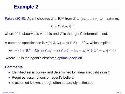
Example 2
Pakes (2010): Agent chooses Z ∈ RdZ from Z ≡ z1, . . . , zK to maximize:
E[π(Y, Z, θ0)|F ]
where Y is observable variable and F is the agent’s information set.
A common specification is π(Y, Z, θ0) = ψ(Y,Z)− Z ′θ0, which implies:
Θ0 = θ ∈ Rdθ : E[((ψ(Y, zj)− ψ(Y, zi))− (zj − zi)′θ)1Z∗ = zi] ≤ 0
where Z∗ is the agent’s observed optimal decision.
Comments• Identified set is convex and determined by linear inequalities in θ.• Requires assumptions on agent’s beliefs.• ψ assumed known, though often separately estimated.
Andres Santos UCSD

Example 3
Luttmer (1996): Under power utility and market frictions, modified Euler:
E[1
1 + ρY −γZ − P ] ≤ 0
with Y future/present consumption, Z ∈ RdZ asset payoff and P prices.
Comments• Constraints strictly convex if Z ≥ 0 and Z > 0 with positive probability.• Resulting identified set for (ρ, γ) is convex.• Big Caveat: Our efficiency bound is for i.i.d. data.
Andres Santos UCSD

General Outline
Preliminaries• Background: support functions and efficiency.• Linear constraints and regularity.
Efficiency• Characterizing sources of irregularity.• Semiparametric efficiency bound for support function.• Show “plug-in” estimator is in fact efficient.
Confidence Regions• Construct bootstrap procedure.• Establish validity of confidence regions.
Andres Santos UCSD

Literature Review
Partial Identification
Manski & Tamer (2002), Manski (2003), Imbens & Manski (2004),Chernozhukov, Hong & Tamer (2007), Romano & Shaikh (2008, 2010),Stoye (2009), Bontemps, Magnac & Maurin (2007), Beresteanu & Molinari(2008), Beresteanu, Molinari & Molchanov (2009), Kaido (2010).
Moment InequalitiesAndrews & Jia (2008), Menzel (2009), Rosen (2009), Andrews & Soares(2010), Bugni (2010), Canay (2010), Pakes (2010).
Efficiency and Regularity
Chamberlain (1987, 1992), Brown & Newey (1998), Newey (2004), Ai &Chen (2009), Chen & Pouzo (2009), Hirano & Porter (2009), Chernozhukov,Lee & Rosen (2009), Song (2010).
Andres Santos UCSD

1 Preliminaries
2 Efficiency
3 Confidence Regions
4 Simulation Evidence
Andres Santos UCSD

Support Function
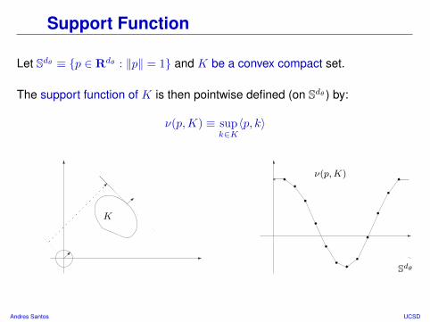
Let Sdθ ≡ p ∈ Rdθ : ‖p‖ = 1 and K be a convex compact set.
The support function of K is then pointwise defined (on Sdθ ) by:
ν(p,K) ≡ supk∈K〈p, k〉
K
ν(p,K)
Sdθ
Andres Santos UCSD

Support Function
Let Sdθ ≡ p ∈ Rdθ : ‖p‖ = 1 and K be a convex compact set.
The support function of K is then pointwise defined (on Sdθ ) by:
ν(p,K) ≡ supk∈K〈p, k〉
K
ν(p,K)
Sdθ
Andres Santos UCSD

Support Function
Let Sdθ ≡ p ∈ Rdθ : ‖p‖ = 1 and K be a convex compact set.
The support function of K is then pointwise defined (on Sdθ ) by:
ν(p,K) ≡ supk∈K〈p, k〉
K
ν(p,K)
Sdθ
Andres Santos UCSD

Support Function
Let Sdθ ≡ p ∈ Rdθ : ‖p‖ = 1 and K be a convex compact set.
The support function of K is then pointwise defined (on Sdθ ) by:
ν(p,K) ≡ supk∈K〈p, k〉
K
ν(p,K)
Sdθ
Andres Santos UCSD

Support Function
Let Sdθ ≡ p ∈ Rdθ : ‖p‖ = 1 and K be a convex compact set.
The support function of K is then pointwise defined (on Sdθ ) by:
ν(p,K) ≡ supk∈K〈p, k〉
K
ν(p,K)
Sdθ
Andres Santos UCSD

Support Function
Let Sdθ ≡ p ∈ Rdθ : ‖p‖ = 1 and K be a convex compact set.
The support function of K is then pointwise defined (on Sdθ ) by:
ν(p,K) ≡ supk∈K〈p, k〉
K
ν(p,K)
Sdθ
Andres Santos UCSD
Support Function
Let Sdθ ≡ p ∈ Rdθ : ‖p‖ = 1 and K be a convex compact set.
The support function of K is then pointwise defined (on Sdθ ) by:
ν(p,K) ≡ supk∈K〈p, k〉
K
ν(p,K)
Sdθ
Andres Santos UCSD

Support Function
Let C(Sdθ ) be the space of bounded continuous functions on Sdθ .
⇒ Every convex compact K is associated with a unique function in C(Sdθ).
Theorem (Hormander) For any two convex compact, K1 and K2:
dH(K1,K2) = supp∈Sdθ
|ν(p,K1)− ν(p,K2)|
where dH(K1,K2) is the Hausdorff distance between the sets K1 and K2.
Norm Equality• Relationship allows for inference; Beresteanu & Molinari (2008).• Equipping C(Sdθ ) with ‖ · ‖∞ implies embedding is isometric.
Andres Santos UCSD
Identified Set
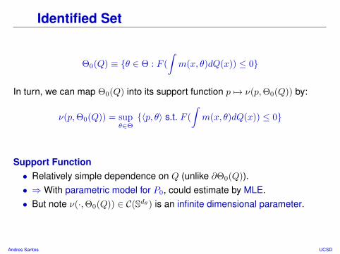
Θ0(Q) ≡ θ ∈ Θ : F (
∫m(x, θ)dQ(x)) ≤ 0
In turn, we can map Θ0(Q) into its support function p 7→ ν(p,Θ0(Q)) by:
ν(p,Θ0(Q)) = supθ∈Θ〈p, θ〉 s.t. F (
∫m(x, θ)dQ(x)) ≤ 0
Support Function• Relatively simple dependence on Q (unlike ∂Θ0(Q)).• ⇒With parametric model for P0, could estimate by MLE.• But note ν(·,Θ0(Q)) ∈ C(Sdθ ) is an infinite dimensional parameter.
Andres Santos UCSD
Efficiency in C(Sdθ)
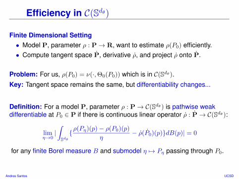
Finite Dimensional Setting• Model P, parameter ρ : P→ R, want to estimate ρ(P0) efficiently.• Compute tangent space P, derivative ρ, and project ρ onto P.
Problem: For us, ρ(P0) = ν(·,Θ0(P0)) which is in C(Sdθ ).Key: Tangent space remains the same, but differentiability changes...
Definition: For a model P, parameter ρ : P→ C(Sdθ ) is pathwise weakdifferentiable at P0 ∈ P if there is continuous linear operator ρ : P→ C(Sdθ ):
limη→0|∫Sdθρ(Pη)(p)− ρ(P0)(p)
η− ρ(P0)(p)dB(p)| = 0
for any finite Borel measure B and submodel η 7→ Pη passing through P0.
Andres Santos UCSD

Convolution Theorem
Theorem (Hayek, LeCam) Under regularity conditions, if ρ : P→ C(Sdθ ) ispathwise weak differentiable at P0 and Tn
L→ G is a regular estimator, then:
G L= G0 + ∆0
for a unique Gaussian process G0 and tight Borel r.v. ∆0 with ∆0 ⊥ G0.
Comments• Since parameter is in C(Sdθ ), estimator Tn converges in C(Sdθ ).• Gaussian process G0 does not depend on Tn, “noise term” ∆0 does.
Intuition: Every regular estimator converges to G0 plus noise ∆0 ...
⇒ An estimator is efficient if it converges in distribution to G0
Andres Santos UCSD
Semiparametric Efficiency
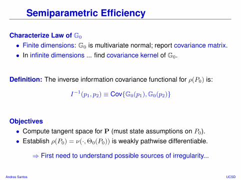
Characterize Law of G0
• Finite dimensions: G0 is multivariate normal; report covariance matrix.• In infinite dimensions ... find covariance kernel of G0.
Definition: The inverse information covariance functional for ρ(P0) is:
I−1(p1, p2) ≡ CovG0(p1),G0(p2)
Objectives• Compute tangent space for P (must state assumptions on P0).• Establish ρ(P0) = ν(·,Θ0(P0)) is weakly pathwise differentiable.
⇒ First need to understand possible sources of irregularity...
Andres Santos UCSD
Differentiability Problems
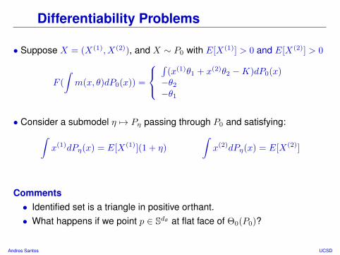
• Suppose X = (X(1), X(2)), and X ∼ P0 with E[X(1)] > 0 and E[X(2)] > 0
F (
∫m(x, θ)dP0(x)) =
∫
(x(1)θ1 + x(2)θ2 −K)dP0(x)−θ2
−θ1
• Consider a submodel η 7→ Pη passing through P0 and satisfying:∫x(1)dPη(x) = E[X(1)](1 + η)
∫x(2)dPη(x) = E[X(2)]
Comments• Identified set is a triangle in positive orthant.• What happens if we point p ∈ Sdθ at flat face of Θ0(P0)?
Andres Santos UCSD

Differentiability Problems
-0.5 0.0 0.5 1.0 1.5
-0.5
0.0
0.5
1.0
1.5
p
Θ0(P0)
Identified Set
Andres Santos UCSD
Differentiability Problems
-0.5 0.0 0.5 1.0 1.5
-0.5
0.0
0.5
1.0
1.5
p
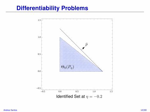
Θ0(Pη)
Identified Set at η = −0.2
Andres Santos UCSD
Differentiability Problems
-0.5 0.0 0.5 1.0 1.5
-0.5
0.0
0.5
1.0
1.5
p
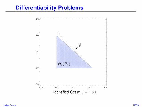
Θ0(Pη)
Identified Set at η = −0.1
Andres Santos UCSD
Differentiability Problems
-0.5 0.0 0.5 1.0 1.5
-0.5
0.0
0.5
1.0
1.5
p
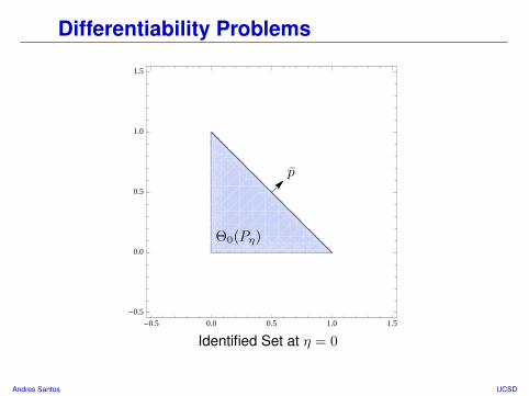
Θ0(Pη)
Identified Set at η = 0
Andres Santos UCSD
Differentiability Problems
-0.5 0.0 0.5 1.0 1.5
-0.5
0.0
0.5
1.0
1.5
p
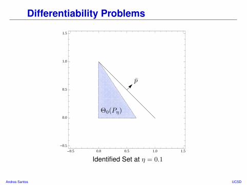
Θ0(Pη)
Identified Set at η = 0.1
Andres Santos UCSD
Differentiability Problems
-0.5 0.0 0.5 1.0 1.5
-0.5
0.0
0.5
1.0
1.5
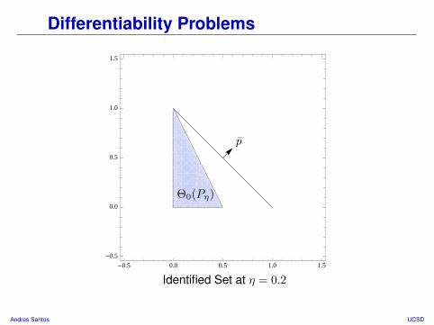
p
Θ0(Pη)
Identified Set at η = 0.2
Andres Santos UCSD
Differentiability Problems
Formally: If p = s/‖s‖ for s = (E[X(1)], E[X(2)]), then along η 7→ Pη,
ν(p,Θ0(Pη)) =
K‖s‖ if η ≥ 0
K‖s‖
E[X(1)](E[X(1)]+η)
if η < 0
Implications• When dθ > 1, slope of linear constraints should not depend on P0.• This is not a problem for strictly convex constraints.• Not a problem in discussed examples.
Next Goal• Restrict P0, F , m so η 7→ ν(·,Θ0(Pη)) is differentiable.• Derive semiparametric efficiency bound and efficient estimator.
Andres Santos UCSD

1 Preliminaries
2 Efficiency
3 Confidence Regions
4 Simulation Evidence
Andres Santos UCSD
Model Details
Problem: Linear constraints may cause support function to be irregular.
Approach: Group constraints into linear and strictly convex ...
For m(x, θ): Let mS : X ×Θ→ RdmS , mL : X → RdmL , A a dFL × dθ matrix.
m(x, θ) ≡ (mS(x, θ)′,mL(x)′, θ′A′)′
For F (v): Let FS : RdmS → RdFS and FL : RdmL → RdFL , let:
F (
∫m(x, θ)dP0(x)) =
(FS(
∫mS(x, θ)dP0(x))
Aθ − FL(∫mL(x)dP0(x))
)where θ 7→ F
(i)S (∫mS(x, θ)dP0(x)) is strictly convex for 1 ≤ i ≤ dFS .
Andres Santos UCSD

Key Assumptions
Assumptions (A)(i) Θ0(P0) is contained in the interior of Θ (relative to Rdθ ).(ii) There exists a θ0 ∈ Θ such that F (E[m(X, θ0)]) < 0.(iii) θ 7→ m(x, θ) is differentiable (but not necessarily in x).(iv) At each θ ∈ ∂Θ0(P0) number of active constraints ≤ dθ.
Discussion• A(i) largely notation. May impose ‖θ‖2 ≤ B or θ(i) ≥ C through F,m.• A(ii) With moment equalities may lose convexity.• A(iii) Allows discontinuous functions of x (e.g. 1Xi = x).• A(iv) analogue to intersection bounds (Hirano & Porter (2009)).
Key: A(ii)-A(iv) implied by linear independence requirement.
Andres Santos UCSD

Lagrangian Representation
ν(p,Θ0(P0)) = supθ∈Θ〈p, θ〉 s.t. F (
∫m(x, θ)dP0(x)) ≤ 0
= supθ∈Θ〈p, θ〉+ λ(p, P0)′F (
∫m(x, θ)dP0(x))
Intuition• Each boundary point of Θ0(P0) is a maximizer for some p ∈ Sdθ .• λ(p, P0) reflects importance of constraints in keeping you inside Θ0(P0).
Reveals Dependence on Pη
⇒ Move along submodel η 7→ Pη ⇒ Changes moment inequalities
⇒ Effect on set depends on constraint importance in shaping ∂Θ0(Pη).
Andres Santos UCSD

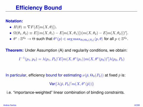
Efficiency Bound
Notation:• H(θ) ≡ ∇F (E[m(X, θ)]).• Ω(θ1, θ2) ≡ E[(m(X, θ1)− E[m(X, θ1)])(m(X, θ2)− E[m(X, θ2)])′].• θ∗ : Sdθ → Θ such that θ∗(p) ∈ arg maxθ∈Θ0(P0)〈p, θ〉 for all p ∈ Sdθ .
Theorem: Under Assumption (A) and regularity conditions, we obtain:
I−1(p1, p2) = λ(p1, P0)′H(θ∗(p1))Ω(θ∗(p1), θ∗(p2))H(θ∗(p2))′λ(p2, P0)
In particular, efficiency bound for estimating ν(p,Θ0(P0)) at fixed p is:
Varλ(p, P0)′∇F (E[m(X, θ∗(p))])m(X, θ∗(p))
i.e. “importance-weighted” linear combination of binding constraints.
Andres Santos UCSD
Efficiency Bound
Notation:• H(θ) ≡ ∇F (E[m(X, θ)]).• Ω(θ1, θ2) ≡ E[(m(X, θ1)− E[m(X, θ1)])(m(X, θ2)− E[m(X, θ2)])′].• θ∗ : Sdθ → Θ such that θ∗(p) ∈ arg maxθ∈Θ0(P0)〈p, θ〉 for all p ∈ Sdθ .
Theorem: Under Assumption (A) and regularity conditions, we obtain:
I−1(p1, p2) = λ(p1, P0)′E[m(X, θ∗(p1))m(X, θ∗(p2))′]λ(p2, P0)
In particular, efficiency bound for estimating ν(p,Θ0(P0)) at fixed p is:
Varλ(p, P0)′m(X, θ∗(p))
i.e. “importance-weighted” linear combination of binding constraints.
Andres Santos UCSD
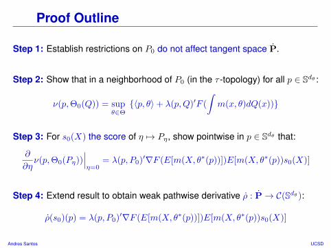
Proof Outline
Step 1: Establish restrictions on P0 do not affect tangent space P.
Step 2: Show that in a neighborhood of P0 (in the τ -topology) for all p ∈ Sdθ :
ν(p,Θ0(Q)) = supθ∈Θ〈p, θ〉+ λ(p,Q)′F (
∫m(x, θ)dQ(x))
Step 3: For s0(X) the score of η 7→ Pη, show pointwise in p ∈ Sdθ that:
∂
∂ην(p,Θ0(Pη))
∣∣∣η=0
= λ(p, P0)′∇F (E[m(X, θ∗(p))])E[m(X, θ∗(p))s0(X)]
Step 4: Extend result to obtain weak pathwise derivative ρ : P→ C(Sdθ ):
ρ(s0)(p) = λ(p, P0)′∇F (E[m(X, θ∗(p))])E[m(X, θ∗(p))s0(X)]
Andres Santos UCSD

Proof Outline (Regularity)
In General: For Λ(p, P0) (set of multipliers), Ξ(p, P0) (set of maximizers):
∂
∂η+ν(p,Θ0(Pη)) = max
θ∗∈Ξ(p,P0)min
λ∈Λ(p,P0)λ′∇F (E[m(X, θ∗)])E[m(X, θ∗)s0(X)]
∂
∂η−ν(p,Θ0(Pη)) = min
θ∗∈Ξ(p,P0)max
λ∈Λ(p,P0)λ′∇F (E[m(X, θ∗)])E[m(X, θ∗)s0(X)]
Intuition• Multiple Lagrange multipliers implies some constraint is redundant.
⇒ Constraints are smooth in η 7→ Pη but relevant ones switch at P0
• Multiple maximizers implies you are on a “flat face” of identified set.⇒ In constraint Aθ − FL(
∫mL(x)dPη), θ∗ does not enter derivative
Andres Santos UCSD
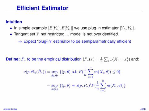
Efficient Estimator
Intuition• In simple example [E[YL], E[YU ]] we use plug-in estimator [YL, YU ].• Tangent set P not restricted ... model is not overidentified.
⇒ Expect “plug-in” estimator to be semiparametrically efficient
Define: Pn to be the empirical distribution (Pn(x) = 1n
∑i 1Xi = x) and:
ν(p,Θ0(Pn)) = supθ∈Θ〈p, θ〉 s.t. F (
1
n
n∑i=1
m(Xi, θ)) ≤ 0
= supθ∈Θ〈p, θ〉+ λ(p, Pn)′F (
1
n
n∑i=1
m(Xi, θ))
Andres Santos UCSD
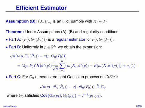
Efficient Estimator
Assumption (B): Xini=1 is an i.i.d. sample with Xi ∼ P0.
Theorem: Under Assumptions (A), (B) and regularity conditions:
• Part A: ν(·,Θ0(Pn)) is a regular estimator for ν(·,Θ0(P0)).
• Part B: Uniformly in p ∈ Sdθ we obtain the expansion:√n(ν(p,Θ0(Pn))− ν(p,Θ0(P0)))
= λ(p, P0)′H(θ∗(p))1√n
n∑i=1
m(Xi, θ∗(p))− E[m(X, θ∗(p))]+ op(1)
• Part C: For G0 a mean zero tight Gaussian process on C(Sdθ ):
√n(ν(·,Θ0(Pn))− ν(·,Θ0(P0)))
L→ G0
where G0 satisfies CovG0(p1),G0(p2) = I−1(p1, p2).
Andres Santos UCSD
Efficient Estimator
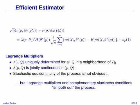
√n(ν(p,Θ0(Pn))− ν(p,Θ0(P0)))
= λ(p, P0)′H(θ∗(p))1√n
n∑i=1
m(Xi, θ∗(p))− E[m(X, θ∗(p))]+ op(1)
Lagrange Multipliers• λ(·, Q) uniquely determined for all Q in a neighborhood of P0.• λ(p,Q) is jointly continuous in (p,Q).• Stochastic equicontinuity of the process is not obvious ...
... but Lagrange multipliers and complementary slackness conditions“smooth out” the process.
Andres Santos UCSD
Back in Θ ...
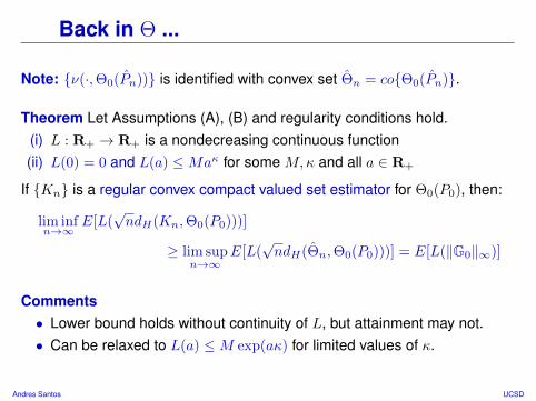
Note: ν(·,Θ0(Pn)) is identified with convex set Θn = coΘ0(Pn).
Theorem Let Assumptions (A), (B) and regularity conditions hold.(i) L : R+ → R+ is a nondecreasing continuous function(ii) L(0) = 0 and L(a) ≤Maκ for some M,κ and all a ∈ R+
If Kn is a regular convex compact valued set estimator for Θ0(P0), then:
lim infn→∞
E[L(√ndH(Kn,Θ0(P0)))]
≥ lim supn→∞
E[L(√ndH(Θn,Θ0(P0)))] = E[L(‖G0‖∞)]
Comments• Lower bound holds without continuity of L, but attainment may not.• Can be relaxed to L(a) ≤M exp(aκ) for limited values of κ.
Andres Santos UCSD

1 Preliminaries
2 Efficiency
3 Confidence Regions
4 Simulation Evidence
Andres Santos UCSD

Bootstrap
Problem: How do we obtain consistent bootstrap for the distribution of G0?
Approach: Perturb estimator of influence function ...
Definition: For random weights Wini=1 define G∗n process pointwise by:
λ(p, Pn)′∇F (1
n
n∑i=1
m(Xi, θ(p)))1√n
n∑i=1
Wim(Xi, θ(p))−1
n
n∑i=1
m(Xi, θ(p))
where θ : Sdθ → Θ satisfies θ(p) ∈ arg maxθ∈Θ0(Pn)〈p, θ〉 for all p ∈ Sdθ .
Why should this work?• If Wi ⊥ Xi, expect to converge to efficient influence function.• Law of G∗n conditional on Xini=1 (but not Wini=1) consistent for G0.
Andres Santos UCSD
Bootstrap
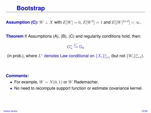
Assumption (C): W ⊥ X with E[W ] = 0, E[W 2] = 1 and E[|W |2+δ] <∞.
Theorem If Assumptions (A), (B), (C) and regularity conditions hold, then:
G∗nL∗
→ G0
(in prob.), where L∗ denotes Law conditional on Xini=1 (but not Wini=1).
Comments:• For example, W ∼ N(0, 1) or W Rademacher.• No need to recompute support function or estimate covariance kernel.
Andres Santos UCSD

Critical Values
Let Ψ0 ⊆ Sdθ and Υ : R→ R. Critical values often are 1− α quantile of:
supp∈Ψ0
Υ(G0(p))
Example 1: Let Ψ0 = Sdθ and Υ(a) = |a|. We need quantiles of:
supp∈Ψ0
Υ(G0(p)) = supp∈Sdθ
|G0(p)|
Example 2: Let Ψ0 = Sdθ and Υ(a) = | − a|+. We need quantiles of:
supp∈Ψ0
Υ(G0(p)) = supp∈Sdθ
| −G0(p)|+
Andres Santos UCSD

Critical Values
AlgorithmStep 1: Compute ν(·,Θ0(Pn)) to obtain p 7→ λ(p, Pn) and p 7→ θ(p).
Step 2: Draw Wini=1 to construct G∗n.
Step 3: Given Hausdorff consistent estimate Ψn for Ψ0 define:
c1−α ≡ infc : P ( supp∈Ψn
Υ(G∗n(p)) ≤ c |Xini=1) ≥ 1− α
Theorem: Under Assumptions (A), (B), (C) and regularity conditions:
c1−αp→ c1−α
Andres Santos UCSD
One Sided Region
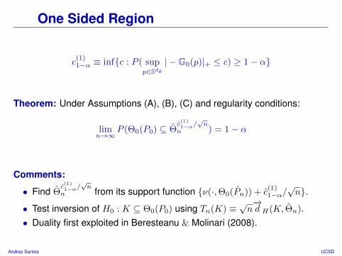
c(1)1−α ≡ infc : P ( sup
p∈Sdθ| −G0(p)|+ ≤ c) ≥ 1− α
Theorem: Under Assumptions (A), (B), (C) and regularity conditions:
limn→∞
P (Θ0(P0) ⊆ Θc(1)1−α/
√n
n ) = 1− α
Comments:
• Find Θc(1)1−α/
√n
n from its support function ν(·,Θ0(Pn)) + c(1)1−α/
√n.
• Test inversion of H0 : K ⊆ Θ0(P0) using Tn(K) ≡√n−→d H(K, Θn).
• Duality first exploited in Beresteanu & Molinari (2008).
Andres Santos UCSD

Two Sided Region
c(2)1−α ≡ infc : P ( sup
p∈Sdθ|G0(p)| ≤ c) ≥ 1− α
Theorem: Under Assumptions (A), (B), (C) and regularity conditions:
limn→∞
P (Θ−c(2)1−α/
√n
n ⊆ Θ0(P0) ⊆ Θc(2)1−α/
√n
n ) = 1− α
Comments:• Provides uniform confidence interval for ∂Θ0(P0).• Test inversion of H0 : K = Θ0(P0) using Tn(K) ≡
√ndH(K, Θn).
Andres Santos UCSD

Region for Parameter
infθ∈Θ0(P0)
lim infn→∞
P (θ ∈ Pn) ≥ 1− α
Standard Approach: Build Pn through test inversion of hypothesis:
H0 : θ ∈ Θ0(P0) H1 : θ /∈ Θ0(P0)
Test Statistic: Use the efficient estimator to test this null hypothesis by:
Hn(θ) ≡√n−→d H(θ, Θn)
Andres Santos UCSD

Region for Parameter
Definition: Let M(θ) be set of maximizers of p 7→ ν(p, θ)− ν(p,Θ0(P0)).
c1−α(θ) ≡ infc : P ( supp∈M(θ)
| −G0(p)|+ ≤ c) ≥ 1− α
Note: Bootstrap with Hausdorff consistent estimate for M(θ) (Kaido 2010).
Theorem: Under Assumptions (A), (B), (C) and regularity conditions:
infθ∈Θ0(P0)
lim infn→∞
P (θ ∈ Pn) ≥ 1− α
where the confidence region is given by Pn ≡ θ ∈ Θ : Hn(θ) ≤ c1−α(θ).
Andres Santos UCSD
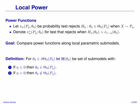
Local Power
Power Functions• Let πn(Pη; θ0) be probability test rejects H0 : θ0 ∈ Θ0(Pη) when X ∼ Pη.• Denote π∗n(Pη; θ0) for test that rejects when Hn(θ0) > c1−α(θ0).
Goal: Compare power functions along local parametric submodels.
Definition: For θ0 ∈ ∂Θ0(P0) let H(θ0) be set of submodels with:
1 If η ≤ 0 then θ0 ∈ Θ0(Pη).2 If η > 0 then θ0 /∈ Θ0(Pη).
Andres Santos UCSD
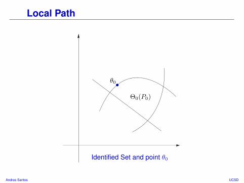
Local Path
Θ0(P0)
θ0•
Identified Set and point θ0
Andres Santos UCSD

Local Path
Θ0(Pη)
θ0•
Identified Set at η = −0.4
Andres Santos UCSD
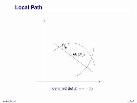
Local Path
Θ0(Pη)
θ0•
Identified Set at η = −0.3
Andres Santos UCSD
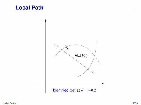
Local Path
Θ0(Pη)
θ0•
Identified Set at η = −0.2
Andres Santos UCSD
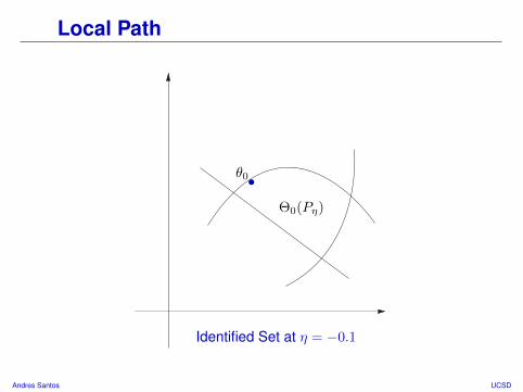
Local Path
Θ0(Pη)
θ0•
Identified Set at η = −0.1
Andres Santos UCSD
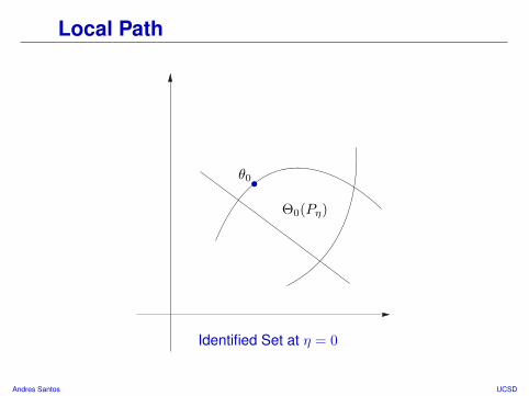
Local Path
Θ0(Pη)
θ0•
Identified Set at η = 0
Andres Santos UCSD

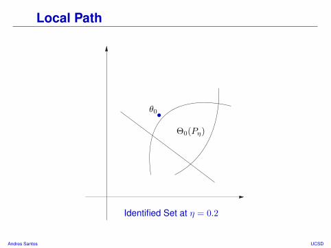
Local Path
Θ0(Pη)
θ0•
Identified Set at η = 0.1
Andres Santos UCSD
Local Path
Θ0(Pη)
θ0•
Identified Set at η = 0.2
Andres Santos UCSD

Local Path
Θ0(Pη)
θ0•
Identified Set at η = 0.3
Andres Santos UCSD

Local Path
Θ0(Pη)
θ0•
Identified Set at η = 0.4
Andres Santos UCSD

Local Power
Theorem: Let Assumptions (A), (B), (C) and regularity conditions hold and
lim supn→∞
πn(Pη/√n; θ0) ≤ α
for every Pη ∈ H(θ0) and η < 0. If M(θ0) = p0, then for any Pη ∈ H(θ0)
lim supn→∞
πn(Pη/√n; θ0) ≤ lim
n→∞π∗n(Pη/
√n; θ0) = 1−Φ
(z1−α − η
E[l(X)s0(X)]√E[G2
0(p0)]
)where s0(x) is the score of η 7→ Pη and l(x) = −λ(p0, P0)′H(θ0)m(x, θ0).
Comments:• Applies to θ0 not at kink of boundaries.• Pη ∈ H(θ0) if and only if E[l(X)s0(X)] > 0.• Weak “size control” requirement ... locality of semiparametric efficiency.
Andres Santos UCSD

Subvectors
Suppose Θ = Θ1 ×Θ2 with Θ1 ⊂ Rdθ1 , Θ2 ⊂ Rdθ2 and θ = (θ1, θ2).
Θ0,M (P0) ≡ θ1 ∈ Θ1 : (θ1, θ2) ∈ Θ0(P0) for some θ2 ∈ Θ2
Key: For p1 ∈ Sdθ1 and (p1, p2) = p ∈ Sdθ1+dθ2 , it follows that:
ν(p1,Θ0,M (P0)) = supθ1∈Θ0,M (P0)
〈p1, θ1〉
= sup(θ1,θ2)∈Θ0(P0)
〈p1, θ1〉+ 〈0, θ2〉 = ν((p1, 0),Θ0(P0))
⇒ The efficient estimator for ν(·,Θ0,M (P0)) is just ν((·, 0),Θ0(Pn)).
⇒ All our results apply to the identified set Θ0,M as well.
Andres Santos UCSD

1 Preliminaries
2 Efficiency
3 Confidence Regions
4 Simulation Evidence
Andres Santos UCSD
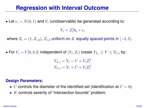
Regression with Interval Outcome
• Let εi ∼ N(0, 1) and Yi (unobservable) be generated according to:
Yi = Z ′iθ0 + εi
where Zi = (1, Zi,2), Zi,2 uniform on K equally spaced points in [−5, 5].
• For Vi ∼ U [0, 0.2] independent of (Yi, Zi) create YLi ≤ Y ≤ YU,i by:
YL,i = Yi − C + ViZ2i
YU,i = Yi + C + ViZ2i
Design Parameters:• C controls the diameter of the identified set (identification at C = 0).• K controls severity of “intersection bounds” problem.
Andres Santos UCSD
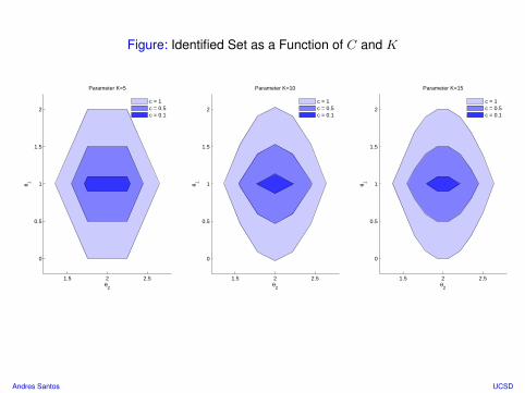
Figure: Identified Set as a Function of C and K
1.5 2 2.5
0
0.5
1
1.5
2
θ2
θ 1
Parameter K=5
c = 1c = 0.5c = 0.1
1.5 2 2.5
0
0.5
1
1.5
2
θ2
θ 1
Parameter K=10
c = 1c = 0.5c = 0.1
1.5 2 2.5
0
0.5
1
1.5
2
θ2
θ 1
Parameter K=15
c = 1c = 0.5c = 0.1
Andres Santos UCSD
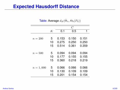
Expected Hausdorff Distance
Table: Average dH(Θn,Θ0(P0))
CK 0.1 0.5 1
n = 200 5 0.153 0.150 0.15110 0.275 0.250 0.25015 0.514 0.361 0.359
n = 500 5 0.094 0.094 0.09410 0.177 0.155 0.15515 0.360 0.218 0.219
n = 1, 000 5 0.066 0.066 0.06610 0.130 0.109 0.10915 0.201 0.154 0.154
Andres Santos UCSD

Expected Inner Hausdorff Distance
Table: Average ~dH(Θn,Θ0(P0))
CK 0.1 0.5 1
n = 200 5 0.137 0.144 0.14410 0.106 0.105 0.10815 0.308 0.045 0.047
n = 500 5 0.088 0.090 0.09010 0.085 0.093 0.09415 0.043 0.051 0.054
n = 1, 000 5 0.063 0.064 0.06410 0.075 0.081 0.08115 0.061 0.055 0.053
Andres Santos UCSD

Expected Outer Hausdorff Distance
Table: Average ~dH(Θ0(P0), Θn)
CK 0.1 0.5 1
n = 200 5 0.150 0.145 0.14510 0.273 0.249 0.25015 0.296 0.359 0.359
n = 500 5 0.092 0.090 0.09010 0.185 0.154 0.15415 0.360 0.218 0.219
n = 1, 000 5 0.064 0.064 0.06410 0.130 0.108 0.10815 0.185 0.154 0.154
Andres Santos UCSD
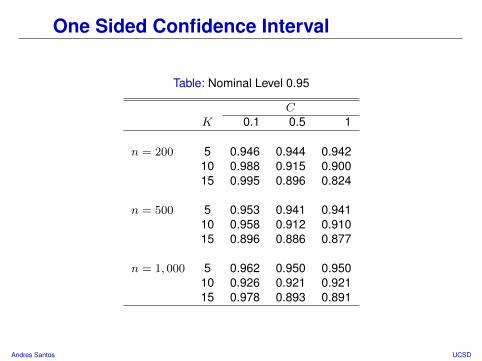
One Sided Confidence Interval
Table: Nominal Level 0.95
CK 0.1 0.5 1
n = 200 5 0.946 0.944 0.94210 0.988 0.915 0.90015 0.995 0.896 0.824
n = 500 5 0.953 0.941 0.94110 0.958 0.912 0.91015 0.896 0.886 0.877
n = 1, 000 5 0.962 0.950 0.95010 0.926 0.921 0.92115 0.978 0.893 0.891
Andres Santos UCSD
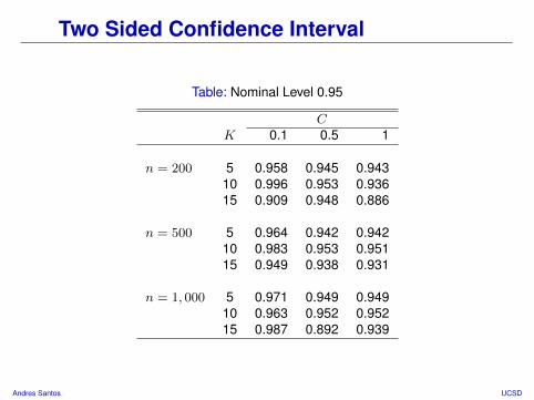
Two Sided Confidence Interval
Table: Nominal Level 0.95
CK 0.1 0.5 1
n = 200 5 0.958 0.945 0.94310 0.996 0.953 0.93615 0.909 0.948 0.886
n = 500 5 0.964 0.942 0.94210 0.983 0.953 0.95115 0.949 0.938 0.931
n = 1, 000 5 0.971 0.949 0.94910 0.963 0.952 0.95215 0.987 0.892 0.939
Andres Santos UCSD
Conclusion
Semiparametric Efficiency• Proposed a notion of semiparametric efficiency.• Characterized sources of irregularity in higher dimensions.• Derived the semiparametric efficiency bound.
Efficient Estimation• Showed “plug-in” estimator is efficient.• Obtained consistent bootstrap procedure.• Employed efficient estimator to construct confidence regions.
Challenges• Efficiency is local concept, often more uniformity is desired.• Sensitivity to “intersection bound” problems in higher dimensions?• Different use of efficient estimator (Imbens & Manski (2004)).• Other efficient estimators may “behave” better ... Sieve MLE? EL?
Andres Santos UCSD


![References - Springer978-0-387-49819-5/1.pdf · References [1] R. Agrawal, M. V. Hegde, and D. Teneketzis. Asymptotically efficient adaptive allocation rules for the multiarmed bandit](https://static.fdocuments.net/doc/165x107/5e05e33742049c30454f8bfa/references-springer-978-0-387-49819-51pdf-references-1-r-agrawal-m-v.jpg)