Asymptotically efficient autoregressive model selection ... · these two alternative methods of...

Ann. Inst, Statist. Math. Vol. 48, No. 3, 577-602 (1996)

ASYMPTOTICALLY EFFICIENT AUTOREGRESSIVE MODEL SELECTION FOR MULTISTEP PREDICTION

R. J. BHANSALI

Department of Statistics and Computational Mathematics, University of Liverpool, Victoria Building, Brownlow Hill, P.O. Box 147, Liverpool L69 3BX, U.K.

(Received March 1, 1994; revised June 5, 1995)

Abst rac t . A direct method for multistep prediction of a stationary time series involves fitting, by linear regression, a different autoregression for each lead time, h, and to select the order to be fitted, kh, from the data. By contrast, a more usual 'plug-in' method involves the least-squares fitting of an initial k-th order autoregression, with k itself selected by an order selection criterion. A bound for the mean squared error of prediction of the direct method is derived and employed for defining an asymptotically efficient order selection for h-step prediction, h > 1; the Sh(k) criterion of Shibata (1980) is asymptotically efficient according to this definition. A bound for the mean squared error of prediction of the plug-in method is also derived and used for a comparison of these two alternative methods of multistep prediction. Examples illustrating the results are given.

Key words and phrases: AIC, FPE, order determination, time series.

1. Introduction

There has been much interest recently in the question of using lead-time dependent estimates or models for multistep prediction of a time series. Thus, Kabaila (1981), Stoica and Soderstrom (1984), Weiss (1991) and Tiao and Xu (1993) consider estimation of the parameters of a specified model separately for each lead time by minimising the sum of squares of the within sample prediction errors. Also, Findley (1983), Gersch and Kitagawa (1983) and Lin and Granger (1994) recommend selecting and fitting a new model for each lead time. Additional references include Greco et al. (1984), Milanese and Tempo (1985), del Pino and Marshall (1986), Hurvich (1987) and Wall and Correia (1989). Grenander and Rosenblatt (1954) and Cox (1961) are two early references in which the h-step prediction constants, h > 1, for a finite predictor are obtained separately for each h by minimising a relevant mean squared error of prediction. Also, Pillai et al. (1992) address the maximum entropy question when the objective is multistep prediction.

577

578 R.J . BHANSALI

From a statistical methodological point of view, the 'direct' method of 'tuning' the parameter estimates or model selection for multistep prediction is quite a general one and it may be applied whenever the notion of a 'true' model generating a time series can be regarded as being implausible and the model fitted for one- step prediction can be viewed simply as a useful approximation for the stochastic structure generating the time series. It is thus probably unsurprising to find that the cited references cover a rather broad range of different classes of time series.

The direct method may be viewed as an alternative to the widely-used 'plug- in' method, see Box and Jenkins (1970), in which the multistep forecasts are obtained from an initial model fitted to the time series by repeatedly using the model with the unknown future values replaced by their own forecasts. Whittle ((1963), p. 36) observed that the plug-in method is optimal in a least-squares sense if the fitted model coincides with that generating the time series, or, in a somewhat restricted sense, for prediction only one step ahead. As, in practice, all fitted models may be incorrect, this observation suggests that for multistep prediction the plug-in method may be improved upon by adopting a different approach and the direct method may be interpreted as being one such approach.

In this paper, a mathematical optimality result for the direct method is established. A result of this type has so far not been available and it contributes towards theoretically underpinning the method in support of which strong empirical evidence has already been presented in the cited references.

Our result is in the context of the autoregressive model fitting approach which provides a natural setting for considering this method because an autoregressive representation exists under weak conditions (Brillinger (1975), p. 78) and the notion of an incorrect model is readily formulated.

On the assumption that T consecutive observations from a discrete-time infinite order autoregressive process, {xt}, are available, a new autoregressive model is selected and fitted for each lead time h _> 1. A direct procedure, involving a linear least-squares regression of xt+ h on xt, x t - 1 , . . . , Xt-k+l, is employed for estimating the autoregressive coefficients. Here, k = kh, say, is a random variable and its value is selected anew for each h. In Section 4, an asymptotic lower bound for the h-step mean squared error of prediction of the direct method is derived, and in Section 5 we show that this bound is attained in the limit if kh is selected by the Sh(k) criterion of Shibata (1980) and also if it is selected by suitable versions of the FPE and AIC criteria of Akaike (1970, 1973).

An asymptotic lower bound for the h-step mean squared error of prediction, h > 1, of the plug-in method when the initial autoregressive order, k = kl, is selected from the data is also derived in Section 6. The results here point to a two-fold advantage in using the direct method: first, the bound on its h-step mean squared error is smaller than that for the plug-in method, and, secondly, the latter bound is not attainable and thus the actual mean squared error for the plug-in method could be larger than this bound. The difference between these two bounds depends upon h and on the autoregressive coefficients generating {xt}. We discuss this point further in Section 7.

In Sections 4 and 5, we also generalise to h > 1 the results for h = 1 of Shibata (1980), who stated, without proof, that an optimality property established by him

MODEL SELECTION FOR MULTISTEP PREDICTION 579

for the Sl(k) criterion would also hold for the Sh(k) criterion when predicting h steps ahead. The generalization involved is non-trivial however, especially a for- mulation of optimality for the direct method with respect to the plug-in method. The technical machinery required is also more complex because for h > 1 an aim of model selection is not to 'whiten' the observed time series so as to produce as residuals a series of (approximately) uncorrelated random variables, but instead it is to produce a series which (approximately) follows a moving average process of order h - 1. Furthermore, we also relax a Gaussian assumption invoked by Shibata (1980, 1981). Indeed, the work of this author serves to clarify the re- lationship between the objectives of consistency and efficiency in order selection by showing that whereas for a finite order process, AIC is not consistent, for an infinite order autoregression it is asymptotically efficient for one-step prediction and for spectral estimation. By contrast, an objective of this paper is to show that this last result does not hold for multistep prediction but that an asymptotically efficient order selection is still possible by selecting a new order for each h with a criterion specifically suggested for this purpose.

2. Preliminaries

Our results hold under a varying combinations of assumptions, and it will be useful to label some of these at the outset.

Suppose that the observed time series is a realization of a stationary process {xt} (t = 0, ± 1 , . . . ) satisfying the following assumptions:

ASSUMPTION 1. resentation

That {xt} possesses a one-sided infinite autoregressive rep-

O<3

E a(j)xt-y = et, a(O) = 1, j=O

in which {et} is a sequence of independent identically distributed random variables, each with mean 0, variance a 2, and the a(j) are absolutely summable real coefficients such that the polynomial

(2.1) A ( z ) = E a ( j ) z J 5 0 , Izl ~ 1. j=O

ASSUMPTION 2. That {xt} does not degenerate to a finite order autoregressive process.

The existence of higher order moments of {et} is also assumed, but the number of moments varies in different results, to ensure flexibility we state the following assumption:

ASSUMPTION 3. For a value of s = So, say, to be further specified

(2.2) E(I¢ I <

580 R. J. B H A N S A L I

Our main Theorems 4.1, 5.1 and 6.1 hold when so -- 16 in Assumption 3, but Proposition 3.1 only with so = 8 and Lemmas 4.1-4.3 with So = 4.

Assumption 1 ensures that {xt} has a representation

o ~

(2.3) xt = ~ b(j)et-j, b(O) = 1, j=o

in which the b(j) are absolutely summable and satisfy (2.1) but with b(j) replacing a(j), and 1 + b(1)z + b(2)z 2 + . . . . [A(z)] -1.

The covariance function of {xt} is defined by R(u) = E(xtxt+u) (t ,u = 0, +1 , . . . ) , its spectral density function by

(2.4) f (#)=(27~) -1 ~ R(s )exp( - i s# ) ,

and the autoregressive transfer function by A(#) = A{exp(- i#)} . For any integer n and all h _ 1, we may write

o o

(2.5) X~+h = -- ~ Ch(j)xn+l-j + Zn+h, j----1

where --¢h(j) is the coefficient of xn+l- j (j = 1, 2 , . . . ) in the linear least-squares predictor, ~ ( h ) , say, of x~+u based on the infinite past, {xt, t <_ n} and

(2.6) h - 1

Z~+h = E b(j)en+h-j j=O

is the h-step prediction error. As in Bhansali (1993),

j - -1

(2.7) Ch(j) = - ~ a ( u ) b ( h - 1 + j - u ) (j = 1 ,2 , . . . ) . u=0

The corresponding mean squared error of prediction is given by

h - 1

(2.8) V(h) = E[{Xn+h -- ~n(h)} 2] ---- a 2 Z b2(j) (h > 1). j=O

Denote the k-th order (direct) linear least-squares predictor of Xn+ h based on the finite past, {Xn, Xn-1, . . . ,Xn-k+l}, k > 1, by

(2.9) XDhk(n) ~ -- Z CDhk(j)Xn+l-j j = l


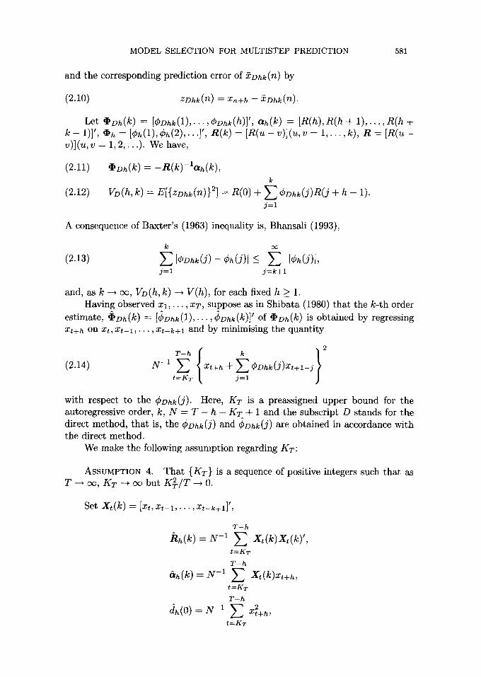
and the corresponding prediction error of XDhk(n) by

(2.10) ZDhk(n) = Xn+h -- ~Vh~(n) .

Let ~Dh(k) = [¢Dhk(1),.. . , CDhk(h)]', ah(k) = JR(h), R(h + 1) , . . . , R(h + k - 1)1', ~h = [¢h(1),¢h(2), . . . ] ' , it(k) = [ R ( u - v)](u,v = 1 , . . . , k ) , R -- [ R ( u - v)l(u,v = 1, 2 , . . . ) . We have,

(2.11)

(2.12)

~Dh(k) -- - R ( k ) - l a h ( k ) , k

VD(h, k) = E[{ZDhk(n)}2J = RiO ) + E CDhk(j)R(j + h - 1). j = l

A consequence of Baxter's (1963) inequality is, Bhansali (1993),

k

(2.13) E ]¢Dhk(j) -- Ch(J)l -< E ICh(J)l, j = l j = k + l

and, as k ~ oc, VD(h, k) ~ V(h), for each fixed h _> 1. Having observed x l , . . . , XT, suppose as in Shibata (1980) that the k-th order

estimate, ~Dh(k) = [¢Dhk(1),.. . , CDhk(k)l' of • ,h (k ) is obtained by regressing Xt+h on xt, x t - 1 , . . . , Xt-k+l and by minimising the quantity

(2.14) N-1 E Xt+h Ac E CDhk(j)XtTl-J t=KT j = l

with respect to the CDhk(j). Here, KT is a preassigned upper bound for the autoregressive order, k, N = T - h - KT + 1 and the subscript D stands for the direct method, that is, the ¢Dhk(j) and ~)Dhk(j) are obtained in accordance with the direct method.

We make the following assumption regarding KT:

ASSUMPTION 4. That {KT} is a sequence of positive integers such that as T ~ oo, KT -"* O0 but K 2 / T ~ O.

Set Xt(k) = [xt, x t - 1 , . . . , Xt-k+l]',

T-h

-~h(k)-= N -1 E Xt(k)Xt(k) ' , t = K T

T-h ah(k) = N-' ~ X,(k)x~+h,

t = K T

T-h

J~(o) = g -1 Z xL~, t = g T

582 R.J. BHANSALI

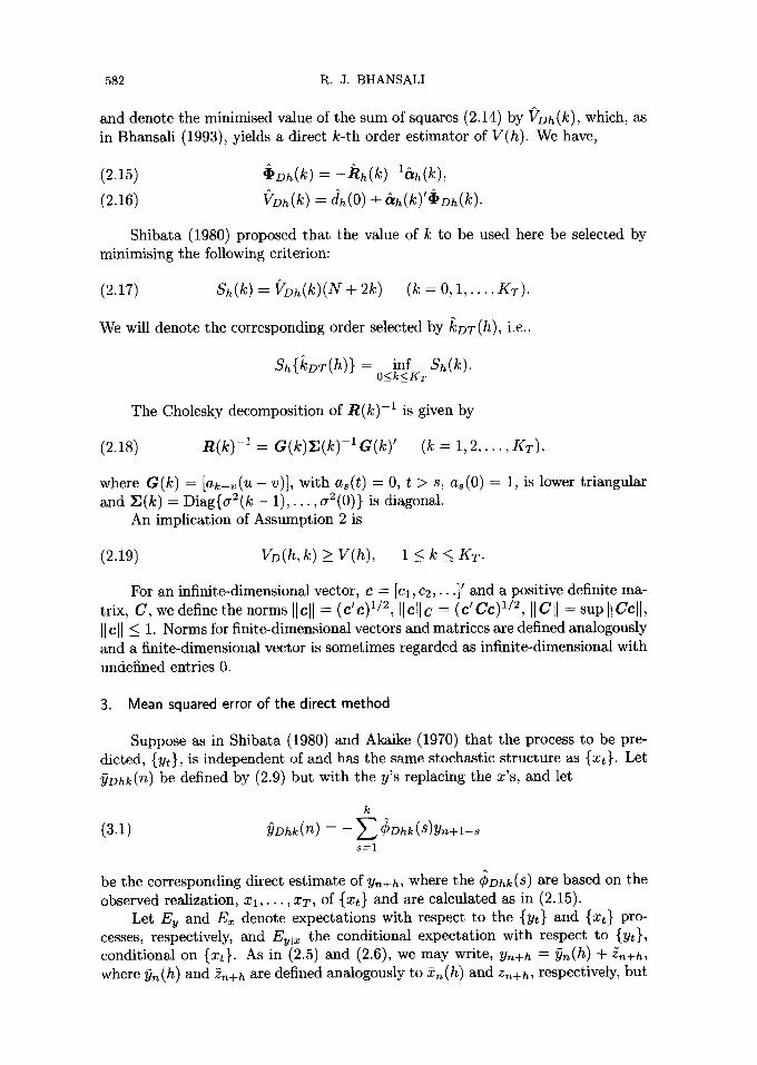
and denote the minimised value of the sum of squares (2.14) by VDh(k), which, as in Bhansali (1993), yields a direct k-th order estimator of V(h). We have,

(2.15) (2.16) VDh(k) = dh(O) +

Shibata (1980) proposed that the value of k to be used here be selected by minimising the following criterion:

(2.17) Sh(k) = VDh(k)(N + 2k) (k = 0, 1 , . . . , KT).

We will denote the corresponding order selected by ~DT(h), i.e.,

Sh{]~DT(h)}= inf Sh(k). O<k<KT

The Cholesky decomposition of R(k) -1 is given by

(2.18) R(k) -1 = C(k)r (k) - l c ( k ) ' (k = 1 , 2 , . . . , K r ) ,

where G(k) = [ak-v(U -- v)], with as(t) = O, t > s, a~(O) = 1, is lower triangular and ~3(k) = Diag{a2(k - 1) , . . . , 62(0)} is diagonal.

An implication of Assumption 2 is

(2.19) VD(h, k) >__ V(h), 1 < k < KT.

For an infinite-dimensional vector, c = [c], c2,...]~ and a positive definite matrix, C, we define the norms II c l l = (c' c) 1/2, II cll c = (c' Cc) 1/2, II C II = sup [t Ccll, Ilcll _< 1. Norms for finite-dimensional vectors and matrices are defined analogously and a finite-dimensional vector is sometimes regarded as infinite-dimensional with undefined entries 0.

3. Mean squared error of the direct method

Suppose as in Shibata (1980) and Akaike (1970) that the process to be predicted, {yt}, is independent of and has the same stochastic structure as {xt}. Let 99hk(n) be defined by (2.9) but with the y's replacing the x's, and let

(3.1) s = l

be the corresponding direct estimate of Yn+h, where the ~Dhk (S) are based on the observed realization, Xl , . . . , XT, of {Xt} and are calculated as in (2.15).

Let Ey and Ex denote expectations with respect to the {yt} and {xt} processes, respectively, and Eylx the conditional expectation with respect to {yt}, conditional on {xt}. As in (2.5) and (2.6), we may write, yn+h = ~n(h) + 5n+h, where ~ln(h) and ~ + h are defined analogously to 2,~(h) and Zn+h, respectively, but


with the y's replacing the x's and with 2~+h denoting the h-step prediction error of the {Yt} process. Hence, on using the identity Ey = ExEyl~ , and noting that under the assumption stated at the beginning of this section, {Yt} is distributed independently of {xt}, the mean squared error of YDhk(n) is given by

(3.2) E~[{~Dhk(n) -- Yn+h} 2]

= - 9 hk(n) -- n+h} 2]

= Ey [{Z~+h }2] + ExEylx [{YDhk (n) -- YDhk (n)}2]

Y(h) + G { l 1 4 D h ( k ) = - ¢ IIR}.

We next develop an asymptotic approximation for the second term to the right of (3.2) by evaluating the probability limit of the quantity occurring inside the curly brackets, since an analytic evaluation of the actual expectation of this term is not straightforward; see Bhansali and Papangelou (1991) for a discussion of this point. To this end, set

(3.3) QD(k) = H4Dh(k) -- "~hl[2R.

It follows from (3.2) that the probability limit of QD (k) provides an approximation to the mean squared error of h-step prediction up to V(h) when Yn+h is predicted by ~]Dhk(n), and, in fact, it could serve as a substitute for this mean squared error.

We may write,

( 3 . 4 ) QD(k) = {VD(h, k) - V(h)} + 114oh(k) -- ~Dh(k)ll~(k ).

The probability limit of the stochastic term on the right of (3.4) is evaluated below in Proposition 3.1; an explicit proof of this proposition is omitted, but one can be constructed from the results of Section 4.

PROPOSITION 3.1. Let {kT} be a sequence of integers such that 1 < kT ~_ KT and kT ---+ ~ as T ---+ ~ , and suppose that Assumptions 1, 2, 3 with So -- 8 and 4 hold. Then, for each fixed h > 1,

(3.5) p l i m (N/kT)fl~Dh(kT) -- ODh(kT)lt2(k) = V(h).

For k = 1, 2 , . . . , KT, let

(3.6) FDhT(k) = {VD(h, k) - Y(h)} + (k /N)Y(h) .

We have the following corollary.

COROLLARY 3.1. Under the assumptions stated in Proposition 3.1,


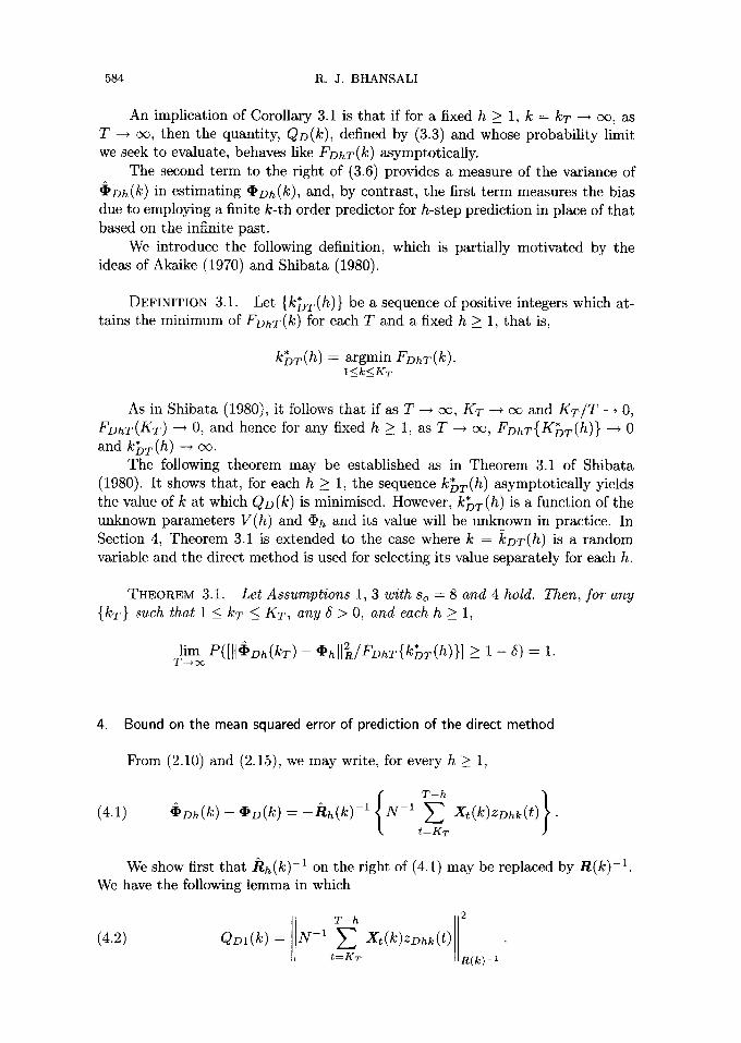
An implication of Corollary 3.1 is that if for a fixed h > 1, k = kT ---+ oe, as T ~ ce, then the quantity, QD(k), defined by (3.3) and whose probability limit we seek to evaluate, behaves like FDhT(k) asymptotically.

The second term to the right of (3.6) provides a measure of the variance of ~Dh(k) in estimating (I~Dh(k), and, by contrast, the first term measures the bias due to employing a finite k-th order predictor for h-step prediction in place of that based on the infinite past.

We introduce the following definition, which is partially motivated by the ideas of Akaike (1970) and Shibata (1980).

DEFINITION 3.1. Let {k*DT(h)} be a sequence of positive integers which at- tains the minimum of FDhT(k ) for each T and a fixed h > 1, that is,

k*DT(h ) = argmin FDhT(k). I<k<KT

As in Shibata (1980), it follows that if as T -* cx~, KT --* oo and K T / T -~ 0, FDhT(KT) --* 0, and hence for any fixed h _> 1, as T -* ce, FDhT{K•T(h)} -~ 0 and k*DT( h ) --* cx~.

The following theorem may be established as in Theorem 3.1 of Shibata (1980). It shows that, for each h ~ 1, the sequence k*DT(h ) asymptotically yields the value of k at which QD(k) is minimised. However, k*DT(h ) is a function of the unknown parameters V(h) and Oh and its value will be unknown in practice. In Section 4, Theorem 3.1 is extended to the case where k = koT(h) is a random variable and the direct method is used for selecting its value separately for each h.

THEOREM 3.1. Let Assumptions 1, 3 with so = 8 and 4 hold. Then, for any {kT} such that 1 <_ kT < KT, any 5 > O, and each h >_ 1,

lira P ( [ l l ~ D h ( k T ) - Ohl I~ /FDhT{k*DT(h)}] >__ 1 - 5 ) = 1. r --* oo

4. Bound on the mean squared error of prediction of the direct method

From (2.10) and (2.15), we may write, for every h > 1,

(4.1) ~Dh(k) - - OD(k) = - R h ( k ) -1 N -1 E Xt(k)ZDhk(t) • t : K T

We show first that Rh(k) -1 on the right of (4.1) may be replaced by R(k) -1. We have the following lemma in which

T - - h 2

(4.2) QDI(k) = N -1 t E-KT Xt(k)ZDhk(t) • R(k)-i


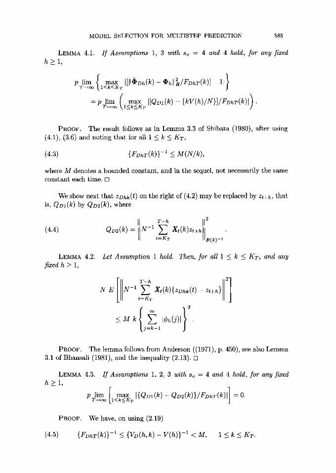
LEMMA 4.1. If Assumptions 1, 3 with so = 4 and 4 hold, for any fixed h> l,

PTli~moo {l<k<KTmax I[H*Dh(k)--~hl]2/FDhT(k)]- 11}

=pli~Ino¢" \l<_k<_Kr( max I[QDI(k) - {kV(h)/N}]/FDhT(k)I).

PROOF. The result follows as in Lemma 3.3 of Shibata (1980), after using (4.1), (3.6) and noting that for all 1 < k < KT,

(4.3) {FDhT(k)} -1 <_ M(N/k) ,

where M denotes a bounded constant, and in the sequel, not necessarily the same constant each time. []

We show next that Z D h k ( t ) on the right of (4.2) may be replaced by Zt+h, that is, QDl(k) by QD2(k), where

(4.4) QD2(k) = N -1 T-hE Xt(k)zt+h 2

t = g T R ( k ) - 1

LEMMA 4.2. Let Assumption 1 hold. Then, for all 1 <_ k <_ KT, and any fixed h > 1,

N E T- -h 2]

g - 1 E Xt(k){ZDhk(t)--Zt+h} t = K T

2

< M k f h(J)l j = k + l

PROOF. The lemma follows from Anderson ((1971), p. 450), see also Lemma 3.1 of Bhansali (1981), and the inequality (2.13). []

LEMMA 4.3. If Assumptions 1, 2, 3 with So = 4 and 4 hold, for any fixed h > l ,

F 1

O.

PROOF. We have, on using (2.19)

(4.5) {FDhT(k)} -1 ~_ {VD(h, k) -- g(h)} -1 < M, 1 < k < KT.


It thus follows from Lemma 4.2 that, with K = KT,

E N -1 T-h 2 ]

max E Xt(k){ZDhk(t) - Zt+h} /FDhT(k) I<k<KT

-- -- t:KT

_< i ~ E i -~ ~ X~(k){z~h~(t) - ~ MKg/T k = i t=KT

and converges to 0 as T --* oc. The lemma may now be established by using the Cauchy-Schwarz inequality and noting that

(4.6) max ][R(k)-~l] ~ M, [] I<k<KT

Now, consider QD2(k). On using the Cholesky decomposition, (2.18), for R(k) -1, we get

(4.7) QD2(k) = E N-1 E Zt+hZmk(t-- u + t) { a 2 ( k - u)} -1. u : l t:KT

We show that Q m ( k ) may be further simplified by replacing z m k ( t - u + 1) and a-2(k - u) by et+l-u and a -2 respectively. Put

(4.8) QD3(k) = E 0"-2 N-1 E Zt+hgt+l-u ' U:I t = K T

LEMMA 4.4. I f Assumptions 1 and 3 with so = 8 hold, for any fixed h > 1,

2

~,u=l v=k--u+l

PROOF. The result follows from (2.13) and the results of Brillinger ((1975), p. 20); see also Lemma 3.2 of Bhansali (1981). []

LEMMA 4.5. tf Assumptions 1, 2, 3 with So = 8, and 4 hold, for any fixed h > l ,

o. L I<k<KT I{QD2(k) - =

PROOF. The lemma follows from (4.5) and Lemma 4.4 on noting that

K

k = l


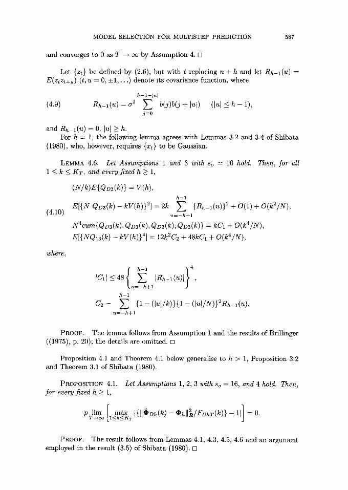
and converges to 0 as T ~ c~ by Assumption 4. []

Let {zt} be defined by (2.6), but with t replacing n + h and let Rh-l(u) = E(ztzt+~) (t, u : 0, + l , . . . ) denote its covariance function, where

h-l-I~l

(4.9) Rh-l(u) = a 2 E b(j)b(j + [u[) (lul _< h - 1), j=o

and Rh-l(u) ---- 0, lul h. For h = 1, the following temma agrees with Lemmas 3.2 and 3.4 of Shibata

(1980), who, however, requires {xt} to be Gaussian.

LEMMA 4.6. 1 < k < KT, and every fixed h >_ 1,

Let Assumptions 1 and 3 with So = 16 hold. Then, for all

(4.10)

(N/k)E{QDa(k)} = V(h), h-1

E[{N QD3(k) -- kV(h)} 21 = 2k E {Rh-l(u)}2 + O(1) + O(k2/N), u------h+l

g4cum{QD3(k), Qo3(k), QD3(k), QDa(k)} = kC1 + O(k4/N),

E[{NQ13(k) - kV(h)} 41 = 12k2C2 + 48kC1 + O(k4/N),

where,

4 tCI[-~ 48//u=-h+l ~ [Rh-l(U)[}~

h-1 C2 = E { 1 - ( lu l /k)}{1- ([ul/g)}2Rh_l(u).

u=-h+l

PROOF. The lemma follows from Assumption 1 and the results of Brillinger ((1975), p. 20); the details are omitted. []

Proposition 4.1 and Theorem 4.1 below generalise to h > 1, Proposition 3.2 and Theorem 3.1 of Shibata (1980).

PROPOSITION 4.1. Let Assumptions 1, 2, 3 with So = 16, and 4 hold. Then, for every fixed h > 1,

PROOF. The result follows from Lemmas 4.1, 4.3, 4.5, 4.6 and an argument employed in the result (3.5) of Shibata (1980). []

588 R. J. BHANSALI

THEOREM 4.1. Let Assumptions 1, 2, 3 with So = 16, and 4 hold. Then, for any random variable, kDT(h), possibly dependent on Xl , . . . , XT, every fixed h > 1 and for any 5 > O,

lim P([ll~Dh{kDT(h)} --OhlI~/FDhT{k*DT(h)}] > 1 --5) = 1. T----* c<~

PROOF. The result follows from Proposition 4.1 and Definition 3.1. []

Theorem 4.1 provides an extension of Corollary 3.1 to the situation in which, for each fixed h > 1, the fitted autoregressive order, k = ~DT(h), say, is a random variable and its selected value is possibly based on the observations, x l , . . . , XT, on {xt}. For this situation, the theorem shows that with any order selection, kDT(h), QD{kDT(h)}, which, as discussed below (3.3), is the substitute mean squared error of prediction up to V(h), is never below F;ghT{kDT(h)} , in probability. In this sense FDhT{k*DT(h)} provides a lower bound for QD(k) when the autoregressive order is selected separately for each h by the direct method. We accordingly define an asymptotically efficient order selection for h-step prediction as follows:

DEFINITION 4.1. For the direct method of fitting autoregression for h-step prediction, h _> 1, an order selection, kDT(h), is said to be asymptotically efficient if

P T l i m ( [ l l ~ D h ( ~ D T ( h ) } -- ~hfl2 /FDhT{k*DT(h)}]) = 1.

5. Asymptotically efficient h-step order selection

We now show that the autoregressive order selection by the Sh(k) criterion, (2.17), is asymptotically efficient in the sense of Definition 4.1, and that small changes to this criterion do not affect this property, and thus obtain appropriate generalisations to the case h > 1 of the corresponding results of Shibata (1980).

For a fixed k > 1, let

(5.1)

We then have

(5.2)

T - h

VDh(k) = N -1 E {ZDhk(t)}2" t=KT

Hence we may write, for all k = 1, 2 , . . . , KT,

Sh(k) = N FDhT(k)+ gl(k)+ g2(k) + g3(k), (5.3)

where

g l ( k ) = 2 k { V D h ( k ) -- V(h)} + N V ( h ) ,

g2(k) {k Y(h) gll~Dh(k ) 2 = - - - - V D h ( k ) l I R ~ ( k ) } ,

g 3 ( k ) = N{?Dh(k) -- VD(h, k ) } .


Proposi t ion 4.1 shows tha t as compared with the first term, the fourth te rm to the right of (5.3) is small, uniformly in 1 < k < KT. Lemma 5.1 below examines the second term.

LEMMA 5.1. I f Assumpt ions 1, 2, 3 with So = 16, and 4 hold, for any fixed h > l ,

p Tlimo~ [l_<l~I_<8~T Ik{VDh(k)-- V ( h ) } / { N F D h T ( k ) } I ] -= O.

PROOF. On using (5.2), we may write

(5.4) If~oh(k) -- V(h)l <_ 114oh(k) -- '~Dh(k) II&h(k

+ If/Dh(k) -- VD(h,k) l + IVD(h, k) -- Y(h) l .

Now, by Lemma 3.3 of Shibata (1980) and our Proposi t ion 4.1,

(5.5) p lim max [kll@Dh(k ) -- ODh(k)ll 2 / {NFDhT(k ) } ] = O. T---*~ I < k < K T h(k)

Also, since E[{f/Dh(k) -- Vm(h, k)} 2] = o ( g - 1 ) , uniformly in 1 < k < KT,

K

E E [ { f / D h ( k ) - VD(h ,k )} 2] <_ M K T / N k = l

and converges to 0 as T --* c~. Thus, in view of (4.5),

(5.6) p l i r n max [ k l f / D h ( k ) - V D ( h , k ) l / { g F D h T ( k ) } ] = O . I <k<KT

The lemma now follows from Assumption 2 and the inequality (4.5). []

Consider now the last te rm to the right of (5.3). If {k~T } is a sequence of positive integers such that k~T ~ oc, as T --+ cx), then for every 1 < k <_ K T and each fixed h > 1 we may write

(5.7) [f/Dh(k~T ) -- VD(h, k~T)] -- If/oh(k) -- VD(h, k)]

= 2['~Dh(k~T) -- "~Dh(k)]'[&h(gT) -- ah(gT)]

+ ['~Dh(k~T) -- @Dh(k ) ] ' {Rh(gT) -- R ( K T ) } • +

where ODh(k~T ) is considered as a K T × 1 vector with undefined entries set equal to zero. We show below that the contr ibution of the two terms to the right of (5.7) is asymptot ical ly negligible.

OC.

and

LEMMA 5.2. Let Assumpt ions 1, 2 and 4 hold and that k~T ---+ co, as T --+ Then, for every fixed h >_ 1, as T -+ oc,

max I{@Dh(k~T) -- ODh(k)} ' {&h(KT) -- a h ( K T ) } / { F D h T ( k ) } l , I <k<KT

590 R . J . B H A N S A L I

m a x I <k< KT

I{ODh(k~T) -- ODh(k ) } ' { t th (KT) -- R ( K T ) }

• { O D h ( k ~ T ) + O D h ( k ) } / { F D h T ( k ) } l

converge in probability to zero•

PROOF. The result follows from (4.5) and the inequality (2.13) by noting that

E{Idh(u) -- R(h - 1 + u)l } ~ M T -1/2,

E { [ D ( T ) ( u , v ) - R ( v - u)l } < M T -1/2, I ~_u~_KT,

1 < u, v <_ KT,

where dh ( u ) denotes t he typical element of &h (KT) and D (T) ( u, v) t hat of ~lh ( KT ). []

We now establish the asymptotic efficiency of the order selected by the Sh(k) criterion for all fixed h > 1. We also show that small changes to the Sh(k) criterion do not affect the asymptotic efficiency of the selected order.

Let k°DT(h) be the order selected by minimising a new criterion,

(5.8) S~(k) = {N + 2k + ~hT(k)}VDh(k), 1 < k < KT,

in which ~'~hT(k) denotes some function of k. The following theorem generalizes Theorems 4.1 and 4.2 of Shibata (1980) to

the case h > 1:

THEOREM 5.1. Let Assumptions 1, 2, 3 with So = 16, and 4 hold, and that ~hT(k) in (5.8) is such that

i) PTlim ~ max I~hT(k)l /N} = 0 ; [ I~k~_KT

ii) plim Ii~km<_aXKT I[~hT(k)- ~hT{k*DT(h)}]/[NFDhT(k)] } %

O.

Then for every fixed h >>_ 1,

a) plim[ll~Dh{kDT(h)}--Oh,l~/FDhT{k*DT(h)}] = 1;

b) the selection, k°DT(h), is asymptotically efficient.

PROOF. To establish a), observe that for all T = 1, 2 , . . . ,

P[Sh{kDT(h)} <_ Sh{k*DT(h)}] = 1•

By (5.3), however, this result implies that

P([FDhT{kDT(h)} --FDhT{k*DT(h)}] ~-- ZhT) = 1,


where 3

zh~ = N -1 ~{9,(kS~(h)) - gi(~.~(h))}. i = 1

Now, Proposition 4.1 and Lemmas 5.1 and 5.2 imply that, as T ~ ec, Z h T "---)

0, in probability. It follows therefore by a standard argument that for any 5 > 0,

lim P([FDhT{]~DT(h)}/FDhT{k*DT(h)}] <_ 1 + 6) = 1. T----* oo

The result a) now follows from Proposition 4.1 by deducing first that this last result and the definition of k*DT(h ) imply that

P Tlim [FDhT{klT(h) } /FDhT{k*DT(h) }] = 1.

Also, b) follows from a), conditions i) and ii) and Proposition 4.1; see also Theorem 4.2 of Shibata (1980). []

As examples of the alternative criteria whose asymptotic efficiency also follows from Theorem 5.1, we have the following:

1) The h-step Final Prediction Error Criterion:

(5.9) FPEh(k ) = VDh(k)(1 + k/T)(1 - k /T) -1 (k = O, 1 , . . . , KT);

2) The h-step information criterion

(5.1o) AICh(k) = T In VDh(k) + 2k (k = 0, 1 , . . . , KT),

which, for h = 1, reduce to the FPE and AIC criteria of Akaike (1970, 1973) respectively; see also Bhansali (1993).

6. Bound for the mean squared error of the plug-in method

Let &(k) -- [&k(1),..., 5k(k)] = ~Dl(k) be the k-th order least-squares estimate of the autoregressive coefficients, and denote the corresponding theoretical parameter by a(k) = [ak(1),.. . ,ak(k)]' = (I)Dl(k), k = 1 , . . . , KT. We also write ~2(k) = yv(1, k).

Now, put

(6.1) -a(k)' ]

~(a) = L / ; - ; l O 2 - 1 J '

where Ik-1 and Ok-1 respectively denote an identity matrix and a vector of zeros of dimension k - 1, and define r(k) analogously but with a(k) replacing 6(k) in (6.1).

592 R . J . B H A N S A L I

As in Yamamoto (1976) and Lewis and Reinsel (1985), the k-th order plug-in estimator, ~ph(k) = [¢Phk (1) , . . . , CPhk (k)]', of the h-step prediction constants is given by, with ek = [1, 0 , . . . , 0] ~,

(6.2) ~ph(k) = -e~F(k) h (h >_ 1),

the corresponding theoretical parameter, ¢Y~Ph (k) -~ [¢Phk(1), '" , CPhlz(k)]' is defined analogously but with r(k) replacing F(k) on the right of (6.2).

Denote the k-th order plug-in predictor of Xn+h, h > 1, based on {xn, x n - ] , . . . , Xn-k+l} by

k

(6.3) 2phk(n) = - ~ ¢phk(j)xn+l-j . j = l

The corresponding h-step prediction error is denoted by

zphk (n) ---- Xn+h -- 2Phk (n)

and the mean squared error of prediction by

Vp(h, k) -~ E[{ZPhk(n)}2].

We have, as in Bhansali (1981),

f (6.4) Vp(h, k) -- IBh_l,k(#)121Ak(#)12f(#)d#, 7~

where, with tOk(j) = e'kr(k)¢ek (j >_ 1),/3k(0) ---- 1, Bh-l ,k(#) denotes the transfer function of the [3k(j) (j = 0, 1 , . . . , h - 1) and Ak(#) that of the ak(j), ak(O) = 1.

We note that if {x~} is a finite autoregressive process of order m, m < k, then, for all h > 1,

ODh(k) = Oph(k) = O(k, h),

where/b(k, h) = [¢h(1), . . . , Ch(k)]' and Ch(J) = 0, j > m, and now ~ph(k) , provides an approximate maximum likelihood estimator of O(k, h), and it is asymptotically efficient for all h > 1; by contrast, ~Dh(k) is asymptotically inefficient for h > 1. Under Assumption 2, however, ODh(k) may be different from Oph(k) and for all k > 1 and each fixed h > 1,

(6.5) Vp(h, k) >_ VD(h, k) >_ V(h).

Moreover, since, as k --~ c~, ak(j) --* a(j), for every fixed j >_ 1, CPhk(j) --~ ¢(j) and Vp(h, k) -+ Y(h), for all h > 1.

Now, as in Section 3, suppose that the process to be predicted, (Yt}, is independent of and has the same stochastic structure as {x~}. Let ~Iphk(n) be defined by (6.3) but with yi replacing xi, i = 1 , . . . , k and let

k

yphk(n) ~ -- Z ~Phk(8)Yn÷l-s s = l


be the corresponding plug-in estimate of Yn+h, where the Cehk(S) are based on x : , . . . , XT and are calculated as in (6.2).

As in (3.2), the mean squared error of prediction of 9phk(n) is given by

Ey[{~)Phk(n) --yn+h} 2] = V(h) + Ex{Qp(k)}

where Qp(k) = IIg~ph(k) -- ~htl~.

Moreover, we now have,

(6.6) Qp(k) = {Vp(h, k) - V(h)} + ll4ph(k) -- Oph(k)ll2(k) + w(k),

where

(6.7) w(k) = 2 { V p h ( k ) - V h } ' R { C p h ( k ) -- V ~ h ( k ) ) .

The probability limits of the stochastic terms on the right of (6.6) and (6.7) may be evaluated as in Section 3 and are given below in Proposition 6.1; for related results see Lewis and Reinset (1985) and Bhansali (1993). To save space, an explicit proof of this proposition is not given.

PROPOSITION 6.1. Under the assumptions stated in Proposition 3.1, for each fixed h > 1,

(6.8)

(6.9)

p l i m ( N / k T ) l t 4 p h ( k T ) -- @ph(kT)ll2R(k) = V(h),

p ~ i m ( N / k ~ ) t w ( k ~ ) l = O.

Now, for k = 1, 2 , . . . , KT, let

(6.10) FphT(k) = {Vp(h, k) - V(h)} + (k/N)V(h).

We have the following corollary, which shows that, if the initial fitted order k = kT, of the plug-in method is a function of T such that kT ~ cxD, as T ~ co, but sufficiently slowly, then, its substitute mean squared error of prediction up to V(h), Qp(k), asymptotically behaves like FphT(k) for each fixed h _> 1.

COROLLARY 6.1. Under the assumptions stated in Proposition 6.1,

It may be observed that Proposition 6.1 and Corollary 6.1 establish for the plug-in method results parallel to Proposition 3.1 and Corollary 3.1 established earlier in Section 3 for the direct method. Moreover, for the plug-in method (6.10) affords an interpretation similar to that of (3.6): thus, the second term to its

594 R.J . BHANSALI

right provides a measure of the variance of ~ p h ( k ) for estimating Oph(k) and the first term measures the bias in using a finite k-th order predictor in place of one based on the infinite past. Now, however, an interesting contrast between these two methods emerges. Proposition 6.1 shows that asymptotically the direct and plug-in methods have the same variance, but, by (6.5), the bias of the plug-in method is never smaller. Thus, for all fixed T and h, and each k > 1,

(6.11) Fphr(k) > FphT(k).

We now extend this last comparison to the situation in which the initial selected order, k, of the plug-in method is a random variable whose value is possibly selected by an order determining criterion. The basic approach we take for this purpose is to derive a lower bound for the mean squared error of prediction of the plug-in method applicable to this situation and then to compare the magnitude of this bound with that derived earlier in Section 4 for the direct method.

We first introduce the following definition, which parallels Definition 3.1, but applies to the plug-in method.

DEFINITION 6.1. Let {k~T(h)} be a sequence of positive integers which at- tains the minimum of FphT(k) for each T and a fixed h _> 1, that is,

k*pT(h ) = argmin FphT(k). I ~ k ~ K T

Like k*DT(h), k*pT(h ) --~ oc, as T ---* oo, since if KT --~ cx~ but K T / T --~ O, FphT(KT) --+ O.

The following theorem establishes for the plug-in method a result similar to that established in Theorem 3.1 for the direct method since it shows that, for each h __ 1, the sequence k*pT(h ) asymptotically yields the values of k that minimises @p(k).

THEOREM 6.1. Let Assumptions 1, 3 with So = 8 and 4 hold. Then, for any {kT} such that 1 ~ kT ~__ KT, any 5 > 0, and each h >_ 1,

lim P([ll '~ph(kT) -- Ohll2/FphT{k*pT(h)}] >_ 1 -- 5) = 1. T----* cx~

However, k*pT(h), like k*DT(h ) is unknown in practice as it is a function of the unknown parameters V(h) and CI, h. Below, we extend Theorem 6.1 to the situation in which k = kPT, say, may be chosen by FPE, AIC or related criteria; the latter include, with a = 2, and h = 1, the criteria to be introduced in Section 7 by (7.3), and the former two are given by (5.9) and (5.10), but with h = 1.

Put fi[ = T - KT,

T - 1

~Z(k ) = ( ~ ) - I E ZDlk(t + 1)Xt(k) , t : K T


and for u ,v = 0 , 1 , . . . , h - 1, let

(6.12) (6.13)

Hu~(k) = r (k)h- l -~R(k)r (k) 'h-~-~,

Luv(k) = R(k)-lHuv(k)R(k) -1,

W~(k) -- Y(k)'£~v(k) Y(k), W ~ ( k ) = Y(k) 'L~(k) Y(k),

where Y ( k ) is obtained from IZ(k) by replacing ZDlk(t+ 1) with et+l and L ~ ( k ) from Luv(k) by replacing R(k) -1 with R(k) -1, and R(k) = Rl(k) is as in (2.15) but with h = 1.

We may write (Bhansali (1981)),

(6.14) h - 1 h - 1

u = 0 v = 0

where/3k(j) = e~r(k)Jek (j = 1 ,2 , . . . , h - 1) and/3k(0) = 1. The following lemma shows that for each fixed (u, v) the error in replacing

W~. (k) by W I ~ (k) is asymptotically negligible.

LEMMA 6.1. Let Assumptions 1, 2, 3 with so = 4 and 4 hold. Then, for every fixed u, v = O, 1 , . . . , h - 1 and each fixed h > 1,

p lim{ I~_k~_KT

I[Wluv(k) - Wuv(k)l/Fp~r(k)l } = 0 .

PROOF. The argument is in two parts: the first step is to show that Y(k) may be replaced by Y ( k ) on the right of (6.12), and the second to show that L~.(k) may also be replaced by L~v(k). To save space the details are omitted, but the method used parallels that given earlier in the proofs of Lemmas 4.1 and 4.2. []

We have, for u,v = 0, 1 , . . . , h - 1,

E { W I ~ ( k ) } = t r {a2R(k ) - lHuv(k )} = W2uv(k), say.

The orders of magnitude of the variance and the fourth central moment of W I ~ (k) are evaluated in the following lemma.

LEMMA 6.2. Let Assumptions 1, 4 and 3 with so = 16 hold. For every u, v = 0, 1 , . . . , h - 1, and each h >_ 1, uniformly in 1 < k < KT,

(6.15) E[{NWluv(k) - W2uv(k)) 2] = O(k) + 0(k2/1~); N 4 cum{Wlu~(k), Wlu~(k), Wluv(k), Wluv(k)} = O(k 2) -~- O(k4/~J); g[{NWluv(k) - W2uv(k)} 4] = O(k 2) Jr- O(k4/~[).

596 R.J . BHANSALI

PROOF. The lemma follows by applying the rules for evaluating cumulants given by Brillinger ((1975), p. 19). []

We now show that W l ~ v ( k ) may be replaced by W2~.(k).

LEMMA 6.3. Let A s s u m p t i o n s 1, 2, 3 with So -- 16, and 4 hold. Then , f o r

u, v = O, 1, . . . , h - 1, and each f ixed h > 1,

[ p l i r a max I { W ~ u . ( k ) - W 2 ~ , ( k ) } / F p h T ( k = O. T--~e~z I <_k<_KT

PROOF. The temma follows from Lemma 6.2; see also result (3.5) of Shibata (1980). []

In the following lemma, an expression for W2uv(k) is obtained by using the Cholesky decomposition (2.18) for R ( k ) -1.

LEMMA 6.4. For every u, v = O, 1 , . . . , h - 1, each f ixed h > 1, and all k > h, with s = h - l - u, t = h - l - v, k = k - m a x ( s , t ) - l , as k --* cx~,

(6.16) cr-2W2u,(k) = M + / _ { I A j ( ~ ) 1 2 / a 2 ( j ) } e x p { i l s - t l # } f ( t t ) d p . 7r

PROOF. We have, on using (2.18), for all u, v

(6.17) a - 2 W 2 ~ , ( k ) = tr{ G ( k ) t H ~ v ( k ) G ( k ) E ( k ) - l } .

The lemma may now be established by noting that the submatrix in the bot tom (k - s) x (k - t) right hand corner of Hu~(k ) has R ( p - q) as its typical element (p = 1 , . . . , k - s; q = 1 , . . . , k - t), and partitioning the matrices G ( k ) ' , G ( k ) and E(k) -1 analogously but ensuring that the dimensions of the relevant submatrices of the matrix product on the right of (6.17) match. []

An implication of Lemma 6.4 is that a uniform bound, valid for all 1 < k < KT, for the mean squared error of the plug-in method may not take a convenient form; a useful approximation may be obtained, however, by restricting the choice of k to the range kT < k < K T , where kT --~ oo as T ---* oo is a sequence of positive integers. This restriction may be justified because the order selected by AIC and related criteria have this property.

LEMMA 6.5. Let A s s u m p t i o n s 1 and 3 with So = 4 hold. For u, v = 0, 1 , . . . , h - 1, each f ixed h > 1 and every divergent sequence { k T } , with 5uv = 1, u = v, 5~v -- O, u T~ v, as T --* oc,

(6.18) I{W2~v(k) - k a 2 6 ~ } / { N F p h T ( k ) } l

MODEL SELECTION FOR MULTISTEP PREDICTION

converges to 0 uniformly in kT < k < K T . I f also Assumpt ions 2, 3 with So = 16 and 4 hold,

(6.19) i) p l i m J~k(U) -- ~k(U)J = O, uniformly in 1 < k ~ KT;

(6.20) ii) [~k(u) -- b(u)J --~ 0, uniformly in kT < k < KT.

597

PROOF. The result (6.18) follows directly from Lemma 6.4, while (6.19) and (6.20) are established recursively in j = 1, 2 , . . . , u on noting that by Proposi t ion

4.1, see also Shibata (1981), k ~-]s=l ]~tk(s) - ak(s)J ~ 0, in probability, uniformly in 1 < k < KT; ]/3k(1) -- b(1)] -- Jak(1) -- a(1)] -~ 0, uniformly in kT < k < KT. []

A bound for the h-step mean squared error of prediction of the plug-in method is given in the following two results which for h = 1 agree with Shibata (1980) but hold wi thout requiring that kT~ o r ~PT, is a divergent sequence.

PROPOSITION 6.2. I f Assumpt ions 1, 2, 3 with So -- 16, and 4 hold,

1 [ { l l 4 p h ( k ) -- V II /FphT(k)} -- 1]1

converges to 0 in probability, uniformly in kT ~_ k < KT , for any divergent sequence { kT } and each fixed h >_ 1.

PROOF. For any divergent sequence, {kT}, as T ~ cx),

I [ l l&Ph(k) -- OPh(k)ll (k) - {kV(h)lN}]lFphT(k)l

converges to 0 in probability, uniformly in kT ~_ k ~_ t (T , by (6.14) and Lemmas 6.1-6.5; also, since, {Vp(h, k) - V(h)} -~ 0, as k --* co, uniformly in kT < k < KT , so does Iw(k) /FphT(k)[ . []

THEOREM 6.2. Let Assumpt ions 1, 2, 3 with So = 16, and 4 hold. For any random variable, k P T , possibly dependent on x l , . . . , XT, and such that k p T ~ 00, as T ~ oc, for any b > O and each h > l,

lim P ( [ ] ] ~ P h T ( k p T ) - - Oh]J2R/FphT{k*pT(h)}] >_ 1 - - 5 ) = 1. T--+ oo

PROOF. The result follows from Proposi t ion 6.1, Definition 3.1 and the assumpt ion tha t kPT --~ (x), as T ----+ oo. []

Theorem 6.2 implies tha t when k is a random variable, the subst i tu te h-step mean squared error of prediction up to V(h ) of the plug-in method, Q p ( k ) , is never below FphT{k*pT(h)} , in probability. For h = 1, as discussed earlier, the bound is a t ta ined asymptot ical ly if k is selected by AIC, or an equivalent criterion.

598 R . J . BHANSALI

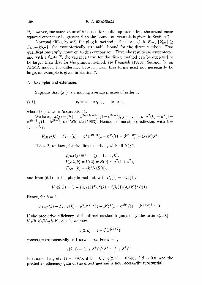
If, however, the same value of k is used for multistep prediction, the actual mean squared error may be greater than the bound; an example is given in Section 7.

A second difficulty with the plug-in method is tha t for each h, FphT{k*pT} > FDhT{k*DT}, the asymptot ical ly at tainable bound for the direct method. Two qualifications apply, however, to this comparison. First, the results are asymptot ic , and with a finite T, the variance term for the direct method can be expected to be larger than that for the plug-in method; see Bhansali (1993). Second, for an A R M A model, the difference between their bias terms need not necessarily be large, an example is given in Section 7.

7. Examples and extensions

Suppose that {xt} is a moving average process of order 1,

(7.1) xt = ~, - / 3 ~ t - 1 , IZl < 1,

where {et} is as in Assumption 1. We have, ak(j) =/3J(1 - /32k-2J+2) / (1 - ~32k+2), j = 1 , . . . , k, a2(k) = a2(1 -

/32k+4)/(1 -/32k+2) see Whit t le (1963). Hence, for one-step prediction, with k =

1,.. . , /~T,

FD1T(k) = Fp1T(]~) = [a2fl~k+2(1 - / 3 2 ) / ( 1 - f12k+2)] + (k/N)a2.

If h = 2, we have, for the direct method, with all k > 1,

¢DUk(j) =-- 0 (j = 1 . . . . , k),

vD(2, k) = v ( 2 ) = R(0) = ~ ( 1 + Z~), F~2~(k) = (k/N)R(0);

and from (6.4) for the plug-in method, with/3k(1) = - ak (1 ) ,

Vp(2, k) = [1 + {/~k(1)}2]a2(k)+ 2~k(1){ak(k)}2R(1).

Hence, for h = 2,

FphT(k) -- FDhT(k) = O-2~2k+2(1 --/32)2(1 -- /32k)/(1 --/32k+2)3 > 0.

If the predictive efficiency of the direct method is judged by the ratio e(h, k) = VD(h, k)/Vp(h, k), h > 1, we have

e(2, k) = 1 - O(~ 2k+2)

converges exponentially to 1 as k --~ cx~. For k = 1,

e(2, 1) = (1 +/3~)4/{~4 + (1 +/3~)4}.

It is seen that , e(2, 1) = 0.975, if /3 = 0.5; e(2, 1) = 0.946, if /3 = 0.8, and the predictive efficiency gain of the direct me thod is not necessarily substantial .


A related question concerns whether or not the same value of k minimises FphT(k) for different values of h. That this is not so may be gleaned by a comparison of FpIT(k) and Fp2T(k), which shows that the values of k minimising the former and the latter do not always coincide. To illustrate this point, we computed the values of these two functions for T = 100, 200, 500, 1000, KT = 30 and several different value of/~. For each (T, t3) combination, the values of k that minimised FphT(k), h ---- i and 2 were determined. To save space, detailed results are omitted, but suffice to say that for ~ < 0.5, the same value of k was selected with h = 1 and h = 2 and for all choices of T. For f~ _> 0.8, however, there was a significant discrepancy between the two orders selected. For example, with T = 1000 and /3 = 0.8, the orders selected with (h = 1, h -- 2) were (10, 7), which increased to (17, 8), for/~ = 0.9 and to (23, 8), for/3 -- 0.95.

One reason why in the moving average example above the gain in predictive efficiency due to the direct method appears small is that the autoregressive coefficients, a(j), decrease to 0 at an exponential rate as j -~ ¢c; the difference between Vp(h, k) and VD(h, k) then vanishes extremely rapidly as k increases and even for moderately small values of k, the numerical value of this difference is negligible. It may be anticipated that this would be so for all "short-memory" time series models since for this class of models, by definition, the difference between Vp (h, k) and VD(h, k) vanishes exponentially as k -~ c~.

Stoica and Nehorai (1989) consider multistep prediction of observations simulated from two linear and two non-linear models by fitting an autoregressive model to the simulated data, but with the coefficients estimated by minimising a linear combination of the squared h-step prediction errors, (2.14), h = 1 , . . . , S, the maximum lead time. They report that if the second-order properties of the simulated model are well approximated by the fitted autoregressive model then the predictive efficiency gain by using this 'multistep error' method is small in comparison with the usual plug-in method; if, however, an underparametrized model is used for prediction then the gain in predictive efficiency can be considerable.

We note that this finding accords with the discussion given above since in the former situation k may be expected to be sufficiently large to ensure that the difference between Vp(h, k) and VD(h, k) is small, but the converse is likely to hold in the latter situation when for small values of k the difference can be substantially in favour of the direct method. It should be pointed out nevertheless that the 'multistep error' method used by these authors is not the same as the direct method examined in this paper, since separate model selection for each lead time has not been considered, rather the same model is used at each lead time but with reestimated parameters and the parameter estimation technique employed is also somewhat different from that described in Section 2. In our view, under the hypothesis that the model generating an observed time series is unknown, the question of model selection for each lead time cannot be separated from that of estimation of the multistep prediction constants and they should be considered together, since the forecasts may be improved by doing both simultaneously instead of only the latter.

An application of the autoregressive model fitting approach for prediction of a 'long-memory' time series has been given by Ray (1993) in whose simulations a

600 R.J. BHANSALI

fractional noise process is forecast up to 20 steps ahead by the plug-in method, but allowing k to vary over a grid of values without recourse to an order determining criterion. Her results endorse the use of autoregressive models for predicting a long- memory process, but indicate a need for considering models of different orders at different lead times, as envisaged in the direct method.

To illustrate the use of these two methods for multistep forecasting of an actual time series, we consider the first 264 observations of the Wolf Annual Sunspot Series, 1700-1963, as given by Wei ((1990), pp. 446-447). Priestley (1981) observes that this series is unlikely to have been generated by a linear mechanism, and, therefore, the present example should point to how the methods might behave with possibly non-linear data.

The plug4n method was applied by fitting an initial 9th order autoregression, the model selected by the FPE2 criterion of Bhansali and Downham (1977), and the direct method by the Sh(k) criterion, (2.17)--the orders of the different autoregressive models selected by this criterion for each h = 1, 2 , . . . , 20 were 9, 9, 17, 17, 16, 15, 14, 13, 12, 11, 2, 3, 3, 3, 7, 6, 11, 10, 9, and 8, respectively. Thus, for this series, the autoregressive order selected varies considerably with the lead time, h, indicating, first, that the series is highly predictable from its own past--even up to twenty steps ahead, and, secondly, that a finite-order autoregressive process probably does not provide an adequate representation for the generating structure of the series. An explanation for why the selected autoregressive order changes so much with different h is, however, not readily given, but it could be related to the highly periodic and possibly non-linear mechanism generating the data. It may be noted also that the estimates (2.15)-(2.16) do not use the same set of observations for different h; nevertheless, under the stationarity assumption, and with T -- 264 observations in total, the possible effects of missing out a small number of 'recent' observations may not be critical.

The forecasts obtained by the plug-in and the direct methods of the Sunspot series for 1964-1983 were compared with the recorded values.

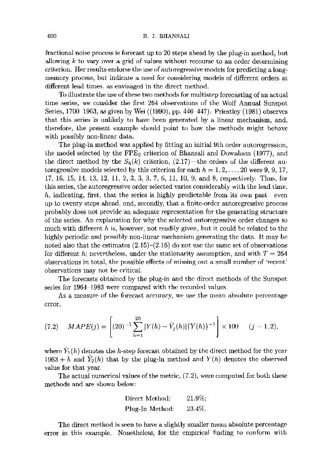
As a measure of the forecast accuracy, we use the mean absolute percentage error,

(7.2) ] M A P E ( j ) = (20) -1 ~ IV(h) - Y j ( h ) l { Y ( h ) } -1 × 100 h = l

(j = 1, 2),

where ]Yl (h) denotes the h-step forecast obtained by the direct method for the year 1963 + h and ]Y2(h) that by the plug-in method and Y(h) denotes the observed value for that year.

The actual numerical values of the metric, (7.2), were computed for both these methods and are shown below:

Direct Method: 21.9%;

Plug-In Method: 23.4%.

The direct method is seen to have a slightly smaller mean absolute percentage error in this example. Nonetheless, for the empirical finding to conform with


the earlier asymptotic results, this difference should be statistically significant, a question we do not pursue here.

The Sh(k), AICh and FPEh criteria may be viewed, see Bhansali and Downham (1977), as special cases with a -- 2 of the following extended criteria in which a > 1 denotes a fixed constant:

(7.3) S(h'~)(k) = (N + ak)VDh(k); FPEh,~(k) = Vnh(k)(1 + ak/N);

AICh~(k) = T ln f/Dh(k) + ak.

Let /¢(DaT)(h) denote the order selected by minimising any of the extended criteria in (7.3). As in Shibata (1980), if the a(j) decrease to 0 exponentially as j --* c~, the selected order would still be asymptotically efficient in the sense of Definition 4.1, but it would not be if the a(j) decrease to 0 geometrically.

Bhansali (1986) defines, with h = 1, a class of generalized penalty functions for which the criteria (7.3) are asymptotically efficient with each fixed a. The argument given there extends to h > 1 by defining a generalized risk function,

F(D~)T(k) = {VD(h, k) - V(k)} + at(k /N)V(h) ,

in which a t > 0 is a fixed constant. It readily follows from Theorems 4.1 and 5.1 that with a = a t + 1 and each h > 1 the order selected by any of the criteria (7.3) is asymptotically efficient with respect to this extended risk function, provided a > 1 remains fixed as T --* c~ and Assumptions 1, 2, 3 with So = 16 and 4 hold.

Acknowledgements

Thanks are due to Dr. David Findley for drawing the problem considered in the paper to the author's attention, and to the referees and an Associate Editor for their helpful comments.

REFERENCES

Akaike, H. (1970). Statistical predictor identification, Ann. Inst. Statist. Math., 22, 203-217. Akaike, H. (1973). Information theory and an extension of the maximum likelihood principle,

2nd International Symposium on Information Theory (eds. B. N. Petrov and F. Csaki), 278-291, Akademia Kiado, Budapest.

Anderson, T. W. (1971). The Statistical Analysis of Time Series, Wiley, New York. Baxter, G. (1963). A norm inequality for a "finite-section" Wiener-Hopf equation, Illinois J.

Math., 7, 97-103. Bhansali, R. J. (1981). Effects of not knowing the order of an autoregressive process on the mean

squared error of prediction--I, J. Amer. Statist. Assoc., 76, 588-597. Bhansali, R. J. (1986). Asymptotically efficient selection of the order by the criterion autore-

gressive transfer function, Ann. Statist., 14, 315-325. Bhansali, R. J. (1993). Estimation of the prediction error variance and an R 2 measure by

autoregressive model fitting, J. Time Ser. Anal., 14, 125-146. Bhansali, R. J. and Downham, D. Y. (1977). Some properties of the order of an autoregressive

model selected by a generalization of Akaike's FPE criterion, Biometrika, 64, 547-551. Bhansali, R. J. and Papangelou, F. (1991). Convergence of moments of least-squares estimators

for the coefficients of an autoregressive process of unknown order, Ann. Statist., 19, 1155- 1162.

602 R . J . BHANSALI

Box, G. E. P. and Jenkins, G. M. (1970). Time Series Analysis: Forecasting and Control, Holden Day, San Francisco.

Brillinger, D. R. (1975). Time Series: Data Analysis and Theory, Holt, New York. Cox, D. R. (1961). Prediction by exponentially weighted moving averages and related methods,

J. Roy. Statist. Soc. Set. B, 23, 414-422. del Pino, G. E. and Marshall, P. (1986). Modelling errors in time series and k-step prediction,

Recent Advances in Systems Modelling (ed. L. Contesse), 87-98, Springer, Berlin. Findley, D. F. (1983). On the use of multiple models for multi-period forecasting, Proceedings of

the Business and Economic Statistics Section, 528-531, American Statistical Association, Washington, D.C.

Gersch, W. and Kitagawa, G. (1983). The prediction of a time series with trends and seasonali- ties, Journal of Business and Economic Statistics, 1,253-264.

Greco, C., Menga, G., Mosca, E. and Zappa, G. (1984). Performance improvements of self-tuning controllers by multistep horizons: the MUSMAR approach, Automatica, 20, 681-699.

Grenander, U. and Rosenblatt, M. (1954). An extension of a theorem of C. Szego and its application to the study of stochastic processes, Trans. Amer. Math. Soc., 76, 112-126.

Hurvich, C. M. (1987). Automatic selection of a linear predictor through frequency domain cross validation, Comm. Statist. Theory Methods, 16, 3199-3234.

Kabaila, P. V. (1981). Estimation based on one step ahead prediction versus estimation based on multi-step ahead prediction, Stochastics, 6, 43 55.

Lewis, R. and Reinsel, G. C. (1985). Prediction of multivariate time series by autoregressive model fitting, J. Multivariate Anal., 16, 393-411.

Lin~ J.-L. and Granger~ C. W. J. (1994). Forecasting from non-linear models in practice, Journal of Forecasting, 13, 1-9.

Milanese, M. and Tempo, R. (1985). Optimal algorithms theory for robust estimation and prediction, IEEE Trans. Automat. Control, AC-30, 730-738.

Pillai, S. U., Shim, T. I. and Benteftifa, M. (1992). A new spectrum extension method that maximizes the multistep minimum prediction error-generalization of the maximum entropy concept, IEEE Transactions on Signal Processing, 40, 142-158.

Priestley, M. B. (1981). Spectral Analysis and Time Series, Academic Press, New York. Ray, B. K. (1993). Modeling long-memory processes for optimal long-range prediction, J. Time

Ser. Anal., 14, 511-526. Shibata, R. (1980). Asymptotically efficient selection of the order of the model for estimating

parameters of a linear process, Ann. Statist., 8, 14~164. Shibata, R. (1981). An optimal autoregressive spectral estimate, Ann. Statist., 9, 300-306. Stoica, P. and Nehorai, A. (1989). On multistep prediction error methods for time series models,

Journal of Forecasting, 8, 357-368. Stoica, P. and Soderstrom, T. (1984). Uniqueness of estimated k-step prediction models of

ARMA processes, Systems Control Lett., 4, 325-331. Tiao, G. C. and Xu, D. (1993). Robustness of MLE for multi-step predictions: the exponential

smoothing case, Biometrika, 80, 623-641. Wall, K. D. and Correia, C. (1989). A preference-based method for forecasting combination,

Journal of Forecasting, 8, 269-292. Wei, W. W. S. (1990). Time Series Analysis, Addison Wesley, Redwood City. Weiss, A. A. (1991). Multi-step estimation and forecasting in dynamic models, J. Econometrics,

46, 135-149. Whittle, P. (1963). Prediction and Regulation by Linear Least-Square Methods, English Univer-

sity Press, London. Yamamoto~ T. (1976). Asymptotic mean square prediction error for an autoregressive model

with estimated coefficients, Applied Statistics, 25, 123-127.

Asymptotically efficient autoregressive model selection ... · these two alternative methods of...

Documents

Transcript of Asymptotically efficient autoregressive model selection ... · these two alternative methods of...