
Asymptotic behaviour of the energy to partially ...rivera/Art_Pub/Tesepere.pdf · Asymptotic...
26
Asymptotic behaviour of the energy to partially viscoelastic materials * Jaime E. Mu˜ noz Rivera Alfonso Peres Salvatierra Abstract In this paper we study models of materials consisting of an elastic part (without memory) and a viscoelastic part, where the dissipation given by the memory is effective. We show that the solutions of the corresponding partial viscoelastic model decay exponentially to zero, provided the relaxation function also decays exponentially, no matter how small is the viscoelastic part of the material. AMS classification code : 35B40, 35L05, 35L70 Keywords and phrases : viscoelasticity, exponential decay, localized damping, materials with memory. 1 Introduction Let us consider a n-dimensional body which in its reference configuration is homogeneous and occupies the open bounded set Ω ⊂ IR n with smooth boundary Γ. Let x 7→ u(x, t) be the position of the material particle x at time t. Then the viscoelastic equation of motion is given by ρu tt - κΔu + Z ∞ 0 g(s) div {a(x)∇u(·,t - s)} ds = f in Ω×]0, ∞[ u(x, t)=0 on ∂ Ω×]0, ∞[= Γ×]0, ∞[ u(x, 0) = u 0 (x), u t (x, 0) = u t (x), in Ω. where ρ is the mass density function, g is the relaxation function and f denotes the body force. Here we are mainly interested on the asymptotic behaviour of the solution u when t tends to infinity. Note that the above model is dissipative, and the dissipation is given by the memory term, where a ≥ 0. The memory is effective only in a part of the body Ω where a> 0. Concerning the exponential stability of dissipative systems, it is well known by now that the solution of the wave equation with frictional damping * Supported by a grant 305406/88-4 of CNPq-BRASIL (To appear in Quarterly of Applied Mathematics) 1
-
Upload
trinhthien -
Category
Documents
-
view
218 -
download
0
Transcript of Asymptotic behaviour of the energy to partially ...rivera/Art_Pub/Tesepere.pdf · Asymptotic...
Asymptotic behaviour of the energy to partially
viscoelastic materials∗
Jaime E. Munoz Rivera Alfonso Peres Salvatierra
Abstract
In this paper we study models of materials consisting of an elastic part (without memory)and a viscoelastic part, where the dissipation given by the memory is effective. We showthat the solutions of the corresponding partial viscoelastic model decay exponentially tozero, provided the relaxation function also decays exponentially, no matter how small is theviscoelastic part of the material.
AMS classification code: 35B40, 35L05, 35L70
Keywords and phrases: viscoelasticity, exponential decay, localized damping, materials with memory.
1 Introduction
Let us consider a n-dimensional body which in its reference configuration is homogeneous and
occupies the open bounded set Ω ⊂ IRn with smooth boundary Γ. Let x 7→ u(x, t) be the
position of the material particle x at time t. Then the viscoelastic equation of motion is given
by
ρutt − κ∆u +
∫ ∞
0g(s) div a(x)∇u(·, t − s) ds = f in Ω×]0,∞[
u(x, t) = 0 on ∂Ω×]0,∞[= Γ×]0,∞[
u(x, 0) = u0(x), ut(x, 0) = ut(x), in Ω.
where ρ is the mass density function, g is the relaxation function and f denotes the body force.
Here we are mainly interested on the asymptotic behaviour of the solution u when t tends to
infinity. Note that the above model is dissipative, and the dissipation is given by the memory
term, where a ≥ 0. The memory is effective only in a part of the body Ω where a > 0.
Concerning the exponential stability of dissipative systems, it is well known by now that the
solution of the wave equation with frictional damping
∗Supported by a grant 305406/88-4 of CNPq-BRASIL (To appear in Quarterly of Applied Mathematics)
1
utt − ∆u + a(x)ut = 0 in Ω×]0,∞[,
u(x, t) = 0, on Γ×]0,∞[,
decays exponentially to zero as time goes to infinity provided a(x) ≥ a0 > 0 a.e. in Ω. In this
case, since a(x) is a positive function, the dissipative effect is working in the whole domain Ω.
In this direction we may ask, whether the damping term a(x)ut continues to be effective when
the function a satifies only a(x) ≥ 0. That is, suppose that the function a(x) vanishes outside
an open subset ω of Ω. Is the dissipative term a(x)ut strong enough to produce the exponential
decay of the solution?. Under what conditions on ω we may expect an uniform rate of decay
for the solution? A first answer to these questions was given in [6], [14], [18], [27]. In those
works the authors proved that the solution of the wave equation with ”local” damping decays
exponentially to zero provided ω is a neighborhood of the boundary Γ. This means that a
dissipation mechanism which is effective over a strategic part of the material is strong enough to
produce exponential rate of decay of the total energy. Such results are connected with Control
Theory. It was proved by Lions [13] that the solution of the wave equation can be controlled
acting only in a neighborhood of the boundary. Roughly speaking, any time that we can control
the solution acting on a part of the material, it is possible to introduce a dissipative mechanism
at the same place producing uniform decay in time of the energy. The methods in Bardos et al.
[1] allow to give a necessary and sufficient condition for the uniform decay of the solutions of the
dissipative wave equation. Namely, this condition requests that every ray of geometric optics
that propagates in Ω and is reflected on the boundary enters the region a > 0 in a uniform
time. In fact, the necessity of this condition is due to the construction of Ralston [22, 23] of
the gaussian beam solutions of the wave equation. Other examples of localized damping are
given by introducing dissipative boundary conditions acting in a part of the boundary. In this
direction there is an extensive literature, see for example [4], [5], [6], [7], [8], [10], [11], [12], [17],
[19], [20], [21], [24], [26], [28] among others.
In this paper we also consider locally distributed dissipation; but this dissipation does not
appear by the introduction of any artificial mechanism. On the contrary, it arises because of
the mixed structure of the material. That is, we consider a body consisting of an elastic and
a viscoelastic part. So, the dissipation is due to the memory effect which works only over a
portion of the material. The one dimensional case is represented in the next picture, but our
analysis applies without restriction on the dimension
2
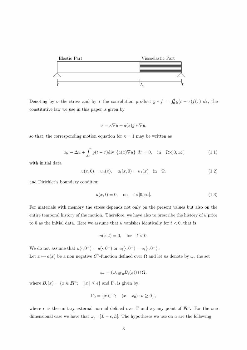
@ @
Viscoelastic PartElastic Part
0 LL1
Denoting by σ the stress and by ∗ the convolution product g ∗ f =∫ t0 g(t − τ)f(τ) dτ , the
constitutive law we use in this paper is given by
σ = κ∇u + a(x)g ∗ ∇u,
so that, the corresponding motion equation for κ = 1 may be written as
utt − ∆u +
∫ t
0g(t − τ)div a(x)∇u dτ = 0, in Ω×]0,∞[ (1.1)
with initial data
u(x, 0) = u0(x), ut(x, 0) = u1(x) in Ω. (1.2)
and Dirichlet’s boundary condition
u(x, t) = 0, on Γ×]0,∞[. (1.3)
For materials with memory the stress depends not only on the present values but also on the
entire temporal history of the motion. Therefore, we have also to prescribe the history of u prior
to 0 as the initial data. Here we assume that u vanishes identically for t < 0, that is
u(x, t) = 0, for t < 0.
We do not assume that u(·, 0+) = u(·, 0−) or ut(·, 0+) = ut(·, 0−).
Let x 7→ a(x) be a non negative C2-function defined over Ω and let us denote by ωε the set
ωε = (∪x∈Γ0Bε(x)) ∩ Ω,
where Bε(x) = x ∈ IRn; ‖x‖ ≤ ε and Γ0 is given by
Γ0 = x ∈ Γ; (x − x0) · ν ≥ 0 ,
where ν is the unitary external normal defined over Γ and x0 any point of IRn. For the one
dimensional case we have that ωε =]L − ε, L[. The hypotheses we use on a are the following
3
x 7→ a(x) ∈ C2(Ω); a(x) =
0 on Ω \ ωε
1 on ωε/2.(1.4)
|∇a(x)|2 ≤ c|a(x)|. (1.5)
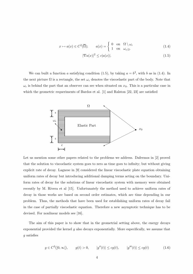
We can built a function a satisfying condition (1.5), by taking a = b2, with b as in (1.4). In
the next picture Ω is a rectangle, the set ωε denotes the viscoelastic part of the body. Note that
ωε is behind the part that an observer can see when situated on x0. This is a particular case in
which the geometric requeriments of Bardos et al. [1] and Ralston [22, 23] are satisfied
ZZ
ZZ
ZZ
ZZ
ZZ
s x0
Ω
s@@I
ωε
-ε
6?
ε
6?
ε
Elastic Part
Let us mention some other papers related to the problems we address. Dafermos in [2] proved
that the solution to viscoelastic system goes to zero as time goes to infinity; but without giving
explicit rate of decay. Lagnese in [9] considered the linear viscoelastic plate equation obtaining
uniform rates of decay but introducing additional damping terms acting on the boundary. Uni-
form rates of decay for the solutions of linear viscoelastic system with memory were obtained
recently by M. Rivera et al [15]. Unfortunately the method used to achieve uniform rates of
decay in those works are based on second order estimates, which are time depending in our
problem. Thus, the methods that have been used for establishing uniform rates of decay fail
in the case of partially viscoelastic equation. Therefore a new asymptotic technique has to be
devised. For nonlinear models see [16].
The aim of this paper is to show that in the geometrial setting above, the energy decays
exponential provided the kernel g also decays exponentially. More especifically, we assume that
g satisfies
g ∈ C3(]0,∞[), g(t) > 0, |g′′(t)| ≤ cg(t), |g′′′(t)| ≤ cg(t) (1.6)
4

−κ0g(t) ≤ g′(t) ≤ κ1g(t) (1.7)
α := 1 −∫ ∞
0g(τ) dτ < 1 (1.8)
To facilitate our analysis, we introduce the following binary operators
g <= ∇u =
∫ t
0g(t − τ)
∫
Ωa(x)|∇u(x, t) −∇u(x, τ)|2 dxdτ
g <= u =
∫ t
0g(t − τ)
∫
Ωa(x)|u(x, t) − u(x, τ)|2 dxdτ
Under the above conditions the main result of this paper is given by
Theorem 1.1 Under the above assumptions on Ω, ω and a and with the kernel g satisfying
(1.6)–(1.8), the weak solution of the viscoelastic equation (1.1)–(1.3), decays exponentially as
time goes to infinity. That is, there exist positive constants c and γ that do not depend on the
initial data, such that
E(t) ≤ cE(0)e−γt
where by E(t) we are denoting the first order energy
E(t) =1
2
∫
Ω|ut|2 +
1 − a(x)
∫ t
0g(τ) dτ
|∇u|2 dx +1
2g <= ∇u.
The method we use here is based on the construction of a functional L for which an inequality
of the form
d
dtL(t) ≤ −cL(t)
holds, with c > 0. To construct such functional L we start from the energy identity. Then,
we look for other functions whose derivatives introduce negative terms such as: −∫
a(x)|ut|2,−∫
a(x)|∇u|2, etc. until we are able to construct the whole energy in the right hand side of the
energy identity. Finally, we take L as the summatory of such functions. Unfortunately, the above
process also introduces terms without definite sign. To overcome this difficulty, we introduce a
new multiplier which allows us to get the appropiate estimates. Finally, we choose carefully the
coefficients of each term of L, such that the resulting summatory satisfies the required inequality.
The remaining part of this article is organized as follows. In the next section 2, we establish
the existence and regularity result to equation (1.1)–(1.3) as well as the energy identity. Section
3 deals with the regularity of the convolution term. Finally in section 4 we show the exponential
decay of the solution of the equation (1.1)–(1.3).
5

2 Existence results and preliminaries
Our starting point is given by the following Lemma
Lemma 2.1 For any v ∈ C1(0, T ;H1(0, L)) we get
∫
Ω
∫ t
0g(t − τ)a(x)∇v dτ · ∇vt dx = −1
2g(t)
∫
Ωa(x)|∇v|2 dx +
1
2g′ <= ∇v
−1
2
d
dt
g <= ∇v −(∫ t
0g dτ
) ∫
Ωa(x)|∇v|2 dx
∫
Ω
∫ t
0g(t − τ)a(x)v dτ · vt dx = −1
2g(t)
∫
Ωa(x)|v|2 dx +
1
2g′ <= v
−1
2
d
dt
g <= v −(∫ t
0g dτ
)∫
Ωa(x)|v|2 dx
Proof.- It is easy to see that
d
dtg <= ∇v = g′ <= ∇v − 2
∫
Ω
∫ t
0g(t − τ)a(x)∇v(τ)dτ · ∇vt(x, t) dτdx
+2
∫ t
0g(t − τ) dτ
∫
Ωa(x)∇v∇vt dx
= g′ <= ∇v − 2
∫
Ω
∫ t
0g(t − τ)a(x)∇v(τ) dτ · ∇vt dx
+d
dt
∫ t
0g(τ) dτ
∫
Ωa(x)|∇v|2 dx
− g(t)
∫
Ωa(x)|∇v|2 dx
This shows our result, the proof of the other identity is similar. <=
It is not difficult to show that there exists only one solution to equation (1.1)–(1.3). We sum-
marize the existence result in the following theorem
Theorem 2.1 Let us suppose that g is a C0-function and that the initial data satisfies
(u0, u1) ∈ H10 (Ω) × L2(Ω),
then, there exists only one weak solution u to equation (1.1)–(1.3) with the following regularity,
u ∈ L∞(0,∞;H10 (Ω)), ut ∈ L∞(0,∞;L2(Ω)).
In addition, if g ∈ C1 and
(u0, u1) ∈ H2(Ω) ∩ H10 (Ω) × H1
0 (Ω);
6

then, there exist only one strong solution u of equation (1.1)–(1.3) satisfying
u ∈ C2−i(0,∞;H10 (Ω) ∩ H i(Ω)), i = 1, 2. u ∈ C2(0,∞;L2(Ω)).
<=
The dissipative property of the viscoelastic equation is summarized in the following Lemma:
Lemma 2.2 Any strong solution of (1.1)–(1.3) satisfies
d
dtE(t) =
1
2g′ <= ∇u − 1
2g(t)
∫
Ωa(x)|∇u|2 dx.
Proof.-Multiplying equation (1.1) by ut and integration over Ω yields
d
dt
∫
Ω
(
|ut|2 + |∇u|2)
dx =
∫
Ωa(x)g ∗ ∇u · ∇ut dx.
From Lemma 2.1 our conclusion follows <=
Lemma 2.2 tells us that the dissipation given by the memory term is effective only on the
support of the function a. We will show in section 4 that such dissipation is enough to produce
the exponential decay of the energy, as time goes to infinity.
3 Regularity of the convolution
Let us denote by ‖ · ‖C0 the norm in C0(Ω). The following Lemma will play an important role
in the sequel.
Lemma 3.1 Let us suppose that g is a positive function satisfying condition (1.8), a ∈ C 0(Ω)
is such that ‖a‖C0 ≤ 1 and finally let us take f ∈ Lp(0, T ;L2(Ω)) with 1 ≤ p < ∞. In this
conditions we have that there exists only one solution v of the Volterra’s equation
v(x, t) −∫ t
0g(t − τ)a(x)v(·, τ) dτ = f(x, t), a.e. (x, t) ∈ Ω×]0, T [
satisfying
v ∈ Lp(0, T ;L2(Ω)).
Besides, there exists a positive constant c independent of T , such that
‖v‖Lp(0,T ;L2) ≤ c‖f‖Lp(0,T ;L2).
7
Proof.-We will use the Picard’s method. Let us denote by
v0 := f, v−1 = 0,
and consider the iterative equation
vµ(x, t) =
∫ t
0g(t − τ)a(x)vµ−1(·, τ) dτ + f(x, t).
Denoting by
wµ = vµ − vµ−1,
we have that
wµ(x, t) =
∫ t
0g(t − τ)a(x)wµ−1(·, τ) dτ,
from where it follows that
‖wµ(t)‖L2 ≤∫ t
0g(t − τ)‖a‖C0‖wµ−1(·, τ)‖L2 dτ.
Using Young’s inequality we get
‖wµ‖Lp(0,T ;L2) ≤(∫ T
0g(τ) dτ
)
‖a‖C0‖wµ−1‖Lp(0,T ;L2)
From where it follows that:
‖wµ‖Lp(0,T ;L2) ≤[
(
∫ T
0g dτ)‖a‖C0
]2
‖wµ−2‖Lp(0,T ;L2)
≤[
(
∫ T
0g dτ)‖a‖C0
]µ
‖w0‖Lp(0,T ;L2)
≤[
(
∫ T
0g dτ)‖a‖C0
]µ
‖f‖Lp(0,T ;L2)
Since (∫ T0 g dτ)‖a‖C0 < 1, then it follows that
∞∑
µ=1
‖wµ‖Lp(0,T ;L2) ≤‖f‖Lp(0,T ;L2)
1 −∫ T0 g dτ‖a‖C0
≤‖f‖Lp(0,T ;L2)
1 − (1 − α)‖a‖C0
.
Where α was defined in (1.8). Recalling that
vµ − v0 =µ∑
i=1
wi,
we conclude that the sequence vµ is convergent. So, there exists a function v ∈ Lp(0, T ;L2(Ω))
for which we have
vµ → v strong in Lp(0, T ;L2(Ω)).
8
Besides, we have that
‖v‖Lp(0,T ;L2) ≤
1
1 − (1 − α)‖a‖C0
+ 1
︸ ︷︷ ︸
:=C
‖f‖Lp(0,T ;L2).
Where C is a positive constant which does not depend on T . To show the uniqueness, let us
suppose that there exists another solution v. Denoting by V = v − v, we have that
V =
∫ t
0g(t − τ)a(x)V (x, τ) dτ.
In particular,
|V | ≤∫ t
0g(t − τ)|a(x)V (x, τ)| dτ.
From Gronwall’s inequality we conclude that V = 0. The proof is now complete <=
In the next Lemma we will show that integration in time is equivalent to remove spatial
derivatives.
Lemma 3.2 Let us suppose that 0 ≤ a(x) ≤ 1 satisfies conditions (1.6)–(1.8) and that g is a
positive function satisfying (1.8). If u is a weak solution of (1.1)–(1.3) satisfying
ut ∈ L∞(0, T ;L2(Ω)), u ∈ L∞(0, T ;H10 (Ω)),
then we have that
g ∗ u ∈ L2(0, T ;H2(Ω))
and
‖g ∗ u‖L2(0,T ;H2) ≤ C
∫ T
0E(t) dt + CE(0). (3.1)
where C is a positive constant independent of T .
Proof.-Applying convolution to equation (1.1) we have
−∆g ∗ u + g ∗ g ∗ div a(x)∇u = −g ∗ utt.
Performing an integration by parts over ]0, t[ we get
g ∗ utt = g(0)ut − g(t)ut(·, 0) +
∫ t
0g′(t − τ)ut dτ := −F.
From the hypotheses we conclude that F ∈ L2(0, T ;L2(Ω)). Denoting by v = g ∗ ∆u, we have
that
−v + a(x)g ∗ v = G (3.2)
9

where
G = F − g ∗ ∇a(x) · ∇u. (3.3)
Applying Lemma 3.1 for p = 2 and since ‖a‖C0 ≤ 1 we conclude that
v ∈ L2(0, T ;L2(Ω)).
Since
∫ T
0
∫
Ω|F |2 dx ≤ 2g(0)2
∫ T
0
∫
Ω|ut|2 dxdt +
∫ T
0g(t)
∫
Ω|u1|2 dxdt +
∫ T
0
∫
Ω|g′ ∗ ut|2 dxdt
︸ ︷︷ ︸
≤∫ T
0|g′| dt
∫ T
0
∫
Ω|ut|2 dx
we have that
‖v‖L2(0,T ;L2(Ω)) ≤ c‖G‖L2(0,T ;L2(Ω))
≤ C
∫ T
0E(t) dt + C
∫ T
0g(t) dtE(0),
which implies that g ∗ ∆u ∈ L2(0, T ;L2(Ω)) from where we obtain
g ∗ u ∈ L2(0, T ;H2(Ω))
Finally, using elliptic regularity, inequality (3.1) follows. The proof is now complete <=
4 Exponential Decay
To show the exponential decay of the solution let us introduce the following functional
I(t) :=
∫
Ωa(x)
ut(g ∗ u)t −1
2g(0)|u|2 −
∫ t
0g dτ |u|2 dx
dx− 1
2g′′ <= u+
1
2
∫
Ωa2(x)|g∗∇u|2 dx.
In these conditions we have:
Lemma 4.1 Under the above conditions and for g ∈ C 3, satisfying conditions (1.6)–(1.8), we
have that for any δ > 0 there exists Cδ satisfying
d
dtI(t) ≤ −g(0)
∫
Ωa(x)|ut|2 dx + δ
∫
Ωa(x)|∇u|2 dx + Cδg <= ∇u
+Cδg(t)
∫
Ωa(x)|∇u|2 dx + Cδ
∫
ωε
∫ t
0g(t − τ)|u(x, t) − u(x, τ)|2 dxdt + Cδ
∫
ωε
|u(x, t)|2 dx.
Here Cδ → ∞ when δ → 0.
10
Proof.-Multiplying equation (1.1) by a(x)(g ∗ u)t we get:
∫
Ωutta(x)(g ∗ u)t dx
︸ ︷︷ ︸
:=I1
−∫
Ω∆ua(x)(g ∗ u)t dx
︸ ︷︷ ︸
:=I2
−∫
Ωa(x)g ∗ ∇u · ∇ a(x)(g ∗ u)t dx
︸ ︷︷ ︸
:=I3
= 0,
from where we have:
I1 =d
dt
∫
Ωuta(x)(g ∗ u)t dx −
∫
Ωuta(x)(g ∗ u)tt dx
=d
dt
∫
Ωuta(x)(g ∗ u)t dx −
∫
Ωuta(x)(g(0)u + g′ ∗ u)t dx
=d
dt
∫
Ωuta(x)(g ∗ u)t dx − g(0)
∫
Ωa(x)|ut|2 dx −
∫
Ωa(x)ut
g′(0)u + g′′ ∗ u
dx
=d
dt
∫
Ωuta(x)(g ∗ u)t dx − g(0)
∫
Ωa(x)|ut|2 dx − g′(0)
2
d
dt
∫
Ωa(x)|u|2 dx
−∫
Ωa(x)utg
′′ ∗ u dx.
Using Lemma 2.1 we get that
∫
Ωa(x)utg
′′ ∗ u dx =1
2g′′′ <= u − 1
2
∫
Ωa(x)|u|2 dx − 1
2
d
dt
g′′ <= u −∫ t
0g dτ
∫
Ωa(x)|u|2 dx
,
from where it follows that
I1(t) =d
dtI0(t) − g(0)
∫
Ωa(x)|ut|2 dx +
1
2g′′(t)
∫
Ωa(x)|u|2 dx − 1
2g′′′ <= u,
where by I0 we are denoting
I0 =
∫
Ωa(x)
ut(g ∗ u)t −g′(0)
2|u|2
dx − 1
2g′′ <= u −
∫ t
0g dτ
∫
Ωa(x)|u|2 dx.
On the other hand:
I2 = −∫
Ωa(x)∆u
g(0)u + g′ ∗ u
dx
=
∫
Ω∇u · ∇
a(x)g(0)u + a(x)g′ ∗ u
dx
=
∫
Ω[∇u · ∇a(x)]g(0)u + g(0)
∫
Ωa(x)|∇u|2 dx +
∫
Ω[∇u · ∇a]g′ ∗ u dx
+
∫
Ωa(x)∇u · g′ ∗ ∇u dx.
Note that
11

∫
Ω[∇u · ∇a]g(0)u +
∫
Ω[∇u · ∇a]g′ ∗ u dx =
g(t)
∫
Ω[∇u · ∇a]u +
∫
Ω∇u · ∇a
∫ t
0g′(t − τ) u(·, τ) − u(·, t) dx.
Similarly, we have
g(0)
∫
Ωa(x)|∇u|2 dx +
∫
Ωa(x)∇u · ∇g′ ∗ u dx =
g(t)
∫
Ωa(x)|∇u|2 dx +
∫
Ωa(x)∇u ·
∫ t
0g′(t − τ) ∇u(·, τ) −∇u(·, t) dx.
Using the above formulas we conclude that I2 may be written as
I2(t) = g(t)
∫
Ω[∇u · ∇a]u +
∫
Ω[∇u · ∇a]
∫ t
0g′(t − τ) u(·, τ) − u(·, t) dx
+g(t)
∫
Ωa(x)|∇u|2 dx +
∫
Ωa(x)∇u ·
∫ t
0g′(t − τ) ∇u(·, τ) −∇u(·, t) dx.
From hypotheses (1.5), (1.7)-(1.8) we have that
∫
Ω[∇u · ∇a]
∫ t
0g′(t − τ) u(·, τ) − u(·, t) dτdx ≤
c
∫
Ω
√a|∇u|
∫ t
0g dτ
1/2 ∫ t
0g(t − τ)|u(·, t) − u(·, τ)|2 dτ
1/2
dx
≤ δ
∫
Ωa(x)|∇u|2 dx + Cδ
∫ t
0
∫
ωε
|u(·, t) − u(·, τ)|2 dxdt.
Using similar ideas to estimate the term
∫
Ωa(x)∇u ·
∫ t
0g′(t − τ) ∇u(·, τ) −∇u(·, t) dxdt
we arrive at
I2(t) ≤ Cδg(t)
∫
Ωa(x)|∇u|2 dx + Cδg <= ∇u + δ
∫
Ωa(x)|∇u|2 dx
+Cδ
∫ t
0
∫
ωε
g′(t − τ)|u(x, t) − u(x, τ)|2 dxdτ,
where δ is a small parameter to be fixed later and Cδ → ∞ as δ → 0. Finally,
12
I3(t) = −∫
Ωag ∗ ∇u · ∇(ag ∗ u)t dx
= −∫
Ωa(x)
∫ t
0g(t − τ)[∇u(·, τ) −∇u(·, t) · ∇a](g ∗ u)t
−∫ t
0g dτ
∫
Ωa(x)[∇u · ∇a](g ∗ u)t dx − 1
2
d
dt
∫
Ωa2|g ∗ ∇u|2 dx
= −∫
Ωa(x)
∫ t
0g(t − τ) ∇u(·, τ) −∇u(·, t) · ∇a(x)
g(0)u + g′ ∗ u
dx
−∫ t
0g dτ
∫
Ωa(x)∇u · ∇a(x)
g(0)u + g′ ∗ u
− 1
2
d
dt
∫
Ωa2|g ∗ ∇u|2 dx.
Using the identity
g(0)u + g′ ∗ u = g(t) +
∫ t
0g′(t − τ) u(·, τ) − u(·, t) dτ
and since a(x) ≤ 1, with the same arguments we used to estimate I2 we have
−∫
Ωa(x)
∫ t
0g(t − τ)[∇u(·, τ) −∇u(·, t) · ∇a] dτ
g(0)u + g′ ∗ u
dx ≤
C
g <= ∇u + g(t)
∫
Ωa(x)|∇u|2 dx
+ δ
∫
Ωa(x)|∇u|2 dx + Cδ
∫
ωε
|u|2 dx.
+Cδ
∫ t
0
∫
ωε
g(t − τ)|u(·, t) − u(·, τ)|2 dxdt,
and
∫ t
0g dτ
∫
Ωa(x)∇u · ∇a(x)
g(0)u + g′ ∗ u
≤
δ
∫
Ωa(x)|∇u|2 dx + Cδ
∫
ωε
|u|2 dx + Cδ
∫ t
0
∫
ωε
g(t − τ)|u(·, t) − u(·, τ)|2 dxdt,
from where it follows that
I3(t) ≤ −1
2
d
dt
∫
Ωa2|g ∗ ∇u|2 dx + Cg <= ∇u + δ
∫
Ωa(x)|∇u|2 dx+
+Cδ
∫
ωε
|u|2 dx + Cδ
∫ t
0
∫
ωε
g(t − τ)|u(·, t) − u(·, τ)|2 dxdt
Since
−I1 = I2 + I3
our conclusion follows by substitution of the relations for Ii, i = 1, 2, 3 into the above identity.
The proof is now complete. <=
13
Lemma 4.2 With the same hypotheses as Lemma 4.1 we have that the solution of equation
(1.1)–(1.3) satisfies,
d
dt
∫
Ωauut dx ≤
∫
Ωa(x)|ut|2 dx − c0
∫
Ωa(x)|∇u|2 dx + c
∫
ωε
|u|2 dx
+Cδ
∫ t
0
∫
ωε
g(t − τ)|u(·, t) − u(·, τ)|2 dxdt.
Proof.-Let us multiply equation (1.1) by a(x)u(x, t) to get
∫
Ωauttu dx
︸ ︷︷ ︸
:=I1
−∫
Ωa(x)u∆u dx
︸ ︷︷ ︸
:=I2
+
∫
Ωdiv ag ∗ ∇u au dx
︸ ︷︷ ︸
:=I3
= 0.
Note that
I1(t) =d
dt
∫
Ωautu dx −
∫
Ωa(x)|ut|2 dx.
On the other hand
I2(t) =
∫
Ω∇u∇au dx
=
∫
Ωu∇u∇a dx +
∫
Ωa(x)|∇u|2 dx
= −1
2
∫
Ω∆a(x)|u|2 dx +
∫
Ωa(x)|∇u|2 dx.
Finally,
I3(t) = −∫
Ωa(x)g ∗ ∇u · ∇ au dx
= −∫
Ωa(x)[g ∗ ∇u · ∇a]u dx −
∫
Ωa2g ∗ ∇u · ∇u dx
= −∫
Ωa(x)[g ∗ ∇u · ∇a]u dx +
∫ t
0g dτ
∫
Ωa2|∇u|2 dx
−∫
Ωa2∫ t
0g(t − τ) ∇u(·, τ) − u(·, t) · ∇u dx.
Summing up I1, I2, and I3 we get
d
dt
∫
Ωauut dx =
∫
Ωa(x)|ut|2 dx −
∫
Ωa(1 − a(x)
∫ t
0g dτ)|∇u|2 dx +
∫
Ω(∆a)|u|2 dx
+
∫
Ωa(x)
∫ t
0g(t − τ) ∇u(·, τ) −∇u(·, t)∇a(x)u dτ dx
+
∫
Ωa2∫ t
0g(t − τ) ∇u(·, τ) −∇u(·, t) dτ∇u dx.
14
Using |∆a(x)| ≤ C our conclusion follows <=
The following Lemma is proved by Lions [13], for convenience we rewrite it here.
Lemma 4.3 Let us denote by qk a C1-function, then any strong solution (u ∈ C i(0, T ;H2−i(Ω))
for i = 0, 1, 2) of the wave equation
utt − ∆u = f, (4.1)
u(x, t) = 0, on Γ×]0,∞[,
satisfies the following identity
d
dt
∫
Ωutqk
∂u
∂xkdx =
∫
Ωfqk
∂u
∂xkdx +
1
2
∫
Γqkνk|
∂u
∂ν|2 dΓ +
∫
Γ
∂u
∂νqk
∂u
∂xkdΓ
+1
2
∫
Ω
∂qk
∂xk
|ut|2 + |∇u|2
dx +
∫
Ω∇u · ∇qk
∂u
∂xkdx.
Proof.-Let us multiply equation (4.1) by qk∂u∂xk
to get
∫
Ωutt − ∆u qk
∂u
∂xkdx =
∫
Ωfqk
∂u
∂xkdx. (4.2)
It is easy to see that
∫
Ωuttqk
∂u
∂xkdx =
d
dt
∫
Ωutqk
∂u
∂xkdx −
∫
Ωutqk
∂ut
∂xkdx
=d
dt
∫
Ωutqk
∂u
∂xkdx − 1
2
∫
Ωqk
∂|ut|2∂xk
dx
=d
dt
∫
Ωutqk
∂u
∂xkdx +
1
2
∫
Ω
∂qk
∂xk|ut|2 dx.
On the other hand
−∫
Ω∆uqk
∂u
∂xkdx = −
∫
Γ
∂u
∂νqk
∂u
∂xkdΓ +
∫
Ω∇u · ∇q
∂u
∂xkdx +
∫
Ω∇u · q ∂∇u
∂xkdx
= −∫
Γ
∂u
∂νqk
∂u
∂xkdΓ +
∫
Ω∇u · ∇q
∂u
∂xkdx +
1
2
∫
Ωqk
∂|∇u|2∂xk
dx
= −∫
Γ
∂u
∂νqk
∂u
∂xkdΓ +
∫
Ω∇u · ∇q
∂u
∂xkdx +
1
2
∫
Γqkνk|∇u|2 dΓ
−1
2
∫
Ω
∂qk
∂xk|∇u|2 dx.
Since u(x, t) = 0 on Γ then we have that
∂u
∂xk= νk
∂u
∂ν,
from where our conclusion follows <=
15
Lemma 4.4 Let us take qk = a2(x)hk, where hk ∈ C2(Ω) is such that hk = νk on Γ. Then we
have that
− d
dt
∫
Ωa2(x)uthk
∂u
∂xkdx ≤ −1
2
∫
Γ0
|∂u
∂ν|2 dΓ + C
∫
Ωa(x)
|ut|2 + |∇u|2
dx
+C
∫
Ωa(x)|h(x) div ag ∗ ∇u |2 dx,
for any solution of equation (1.1)–(1.3)
Proof.-From Lemma 4.3 applied to qk = a2(x)hk we have
− d
dt
∫
Ωa2hkut
∂u
∂xkdx = −
∫
Ωfa2(x)hk
∂u
∂xkdx =
∫
Γa2(x)hkνk|
∂u
∂ν|2 dx
+1
2
∫
Ω
∂a2(x)hk
∂xk
|ut|2 − |∇u|2
dx +
∫
Ω∇u · ∇a2hk
∂u
∂xkdx.
Since a = 1 on Γ0 and hk = νk on Γ, using the Cauchy-Schwarz inequality, our conclusion
follows. <=
Let us denote by LN (t) the functional
LN (t) = NE(t) + I(t) +g(0)
2
∫
Ωa(x)uut dx − δ0
∫
Ωa2(x)uthk
∂u
∂xkdx.
In these conditions we get
Lemma 4.5 Under the above notations we have
d
dtLN (t) ≤ −κ0
∫
Ωa(x)
|ut|2 + |∇u|2
dx − N
2
g <= ∇u + g(t)
∫
Ωa(x)|∇u|2 dx
(4.3)
−δ0
2
∫
Γ|∂u
∂ν|2 dΓ + Cδ0
∫
Ωa(x)|h(x) div ag ∗ ∇u |2 dx + C
∫
ωε
|u|2 dx
+C
∫ t
0
∫
ωε
g(t − τ)|u(x, t) − u(x, τ)|2 dxdτ.
Proof.-From Lemma 4.1 and Lemma 4.2 we get that
d
dt
I(t) +g(0)
2
∫
Ωa(x)uut dx
≤ −g(0)
2
∫
Ωa(x)|ut|2 dx − (C − δ)
∫
Ωa(x)|∇u|2 dx
+C
∫
ωε
|u|2 dx + Cδ
g <= ∇u + g(t)
∫
Ωa(x)|∇u|2 dx
+C
∫ t
0
∫
ωε
g(t − τ)|u(x, t) − u(x, τ)|2 dxdτ.
16
So, taking δ small enough we get that there exists a positive constant k0 such that
d
dt
I(t) +g(0)
2
∫
Ωa(x)uut dx
≤ −2κ0
∫
Ωa(x)|ut|2 dx +
∫
Ωa(x)|∇u|2 dx
+C
∫
ωε
|u|2 dx + Cδ
g <= ∇u + g(t)
∫
Ωa(x)|∇u|2 dx
+C
∫ t
0
∫
ωε
g(t − τ)|u(x, t) − u(x, τ)|2 dxdτ.
Using Lemma 2.2, Lemma 4.4 and the above inequality we arrive at
d
dtLN (t) ≤ −κ0
∫
Ωa(x)|ut|2 dx +
∫
Ωa(x)|∇u|2 dx
− ε
2
∫
Γ|∂u
∂ν|2 dΓ
−(N − Cδ)
g <= ∇u + g(t)
∫
Ωa(x)|∇u|2 dx
+ C
∫
ωε
|u|2 dx
+Cε
∫
Ωa(x)|h(x) div ag ∗ ∇u |2 dx + C
∫ t
0
∫
ωε
g(t − τ)|u(x, t) − u(x, τ)|2 dxdτ.
Therefore taking N > 2Cδ, we get
d
dtLN(t) ≤ −κ0
∫
Ωa(x)|ut|2 dx +
∫
Ωa(x)|∇u|2 dx
− ε
2
∫
Γ|∂u
∂ν|2 dΓ
−N
2
g <= ∇u + g(t)
∫
Ωa(x)|∇u|2 dx
+ C
∫
ωε
|u|2 dx
+Cδ0
∫
Ωa(x)|h(x) div ag ∗ ∇u |2 dx +
∫ t
0
∫
ωε
g(t − τ)|u(x, t) − u(x, τ)|2 dxdτ.
The proof is now complete <=
Lemma 4.6 Let us suppose that u is the weak solution of (1.1)–(1.3), then there exists a positive
constant C, independent of T , such that
∫ T
0
∫
Ωa(x)|div ag ∗ ∇u |2 dxdt ≤ C
∫ T
0
∫
Ωa(x)
|ut|2 + |∇u|2
dxdt (4.4)
+C
∫ T
0g(t) dtE(0),
∫ T
0
∫
Ω|div ag ∗ ∇u |2 dxdt ≤ C
∫ T
0E(t)dt + C
∫ T
0g(t) dtE(0). (4.5)
Proof.-Note that
div ag ∗ ∇u = ∇a · ∇u + ag ∗ ∆u.
As in the proof of Lemma 3.2, v =√
ag ∗ ∆u satisfies
−v + a(x)g ∗ v =√
aG
17

where G is given by (3.3). Using similar arguments, we conclude that
‖v‖2L2(0,T ;L2) ≤
∫ T
0
∫
Ωa(x)|G|2 dxdt
≤∫ T
0
∫
Ωa(x)
|ut|2 + |∇u|2
dxdt + C
∫ T
0g dtE(0).
Therefore it follows that
∫ T
0
∫
Ωa(x)| div ag ∗ ∇u |2 dxdt ≤ C
∫ T
0
∫
Ωa(x)
|ut|2 + |∇u|2
dxdt + C
∫ T
0g(t) dtE(0),
for a positive constant C. The proof is now complete <=
Lemma 4.7 Let us suppose that ϕ is a weak solution of the wave equation
ϕtt − ∆ϕ = 0
ϕ(x, 0) = ϕ0, ϕt = ϕ1
ϕ(x, t) = 0, on Σ = Γ×]0,∞[.
Then, for x0 ∈ IRn and T > 2R(x0), there exists a positive constant C > 0 for which we have
E(0) ≤ C
∫ T
0
∫
ω|ϕt|2 + |∇ϕ|2 dxdt
for any (ϕ0, ϕ1) ∈ H10 (Ω) × L2(Ω) where
R(x0) = maxx∈Ω
|n∑
k=1
(xk − x0k)
2|1/2
Proof.-See [13] Lemma 2.3, Chapter VIII, pag 411. <=
Our next step is to estimate the term∫
ω |u|2 dx. To do this we will use the following Lemma
Lemma 4.8 Let us suppose that u is a weak solution of (1.1)–(1.3), then for any ε > 0 there
exist a positive constant Cε for which we have
∫ T
0
∫
Ω|u|2 dxdt ≤ Cε
∫ T
0g(t)
∫
Ωa(x)|∇u|2 dxdt +
∫ T
0g <= ∇u dt
+ε
∫ T
0
∫
Ωa(x)
|∇u|2 + |ut|2 + | div ag ∗ ∇u|2
dxdt,
∫ T
0
∫
Ω|g ∗ ∇u|2 dxdt ≤ Cε
∫ T
0g(t)
∫
Ωa(x)|∇u|2 dxdt +
∫ T
0g <= ∇u dt
+ε
∫ T
0
∫
Ωa(x)
|∇u|2 + |ut|2 + | div ag ∗ ∇u|2
dxdt,
18
and
∫ T
0
∫ t
0
∫
Ωg(σ − t)|u(x, σ) − u(x, t)|2 dxdσdt ≤
Cε
∫ T
0g(t)
∫
Ωa(x)|∇u|2 dxdt +
∫ T
0g <= ∇u dt
+ε
∫ T
0
∫
Ωa(x)
|∇u|2 + |ut|2 + | div ag ∗ ∇u|2
dxdt,
provided T is large enough.
Proof.-We argue by contradiction. Suppose that there exists ε0 > 0 and a sequence of
functions such that
∫ T
0
∫
Ω|uν |2 dxdt ≥ ν
∫ T
0g(t)
∫
Ωa(x)|∇uν |2 dxdt +
∫ T
0g <= ∇uν dt
+ε0
∫ T
0
∫
Ωa(x)
|∇uν |2 + |uνt |2 + | div ag ∗ ∇u|2
dxdt, (4.6)
for ν → ∞. By the linearity of the problem we may suppose that
∫ T
0
∫
Ω|uν |2 dxdt = 1, ∀ν ∈ IN. (4.7)
So, we get that
g(t)a(x)|∇uν |2+
∫ t
0a(·)g(t−τ)|uν(·, τ)−uν(·, t)|2 dτ → 0 strongly in L1(]0,∞[×Ω).
(4.8)
Let us decompose uν into:
uν = wν + vν ,
where
wνtt − ∆wν = −div ag ∗ ∇uν (bounded in L2(0, T ;L2(Ω))).
wν(x, 0) = 0, wνt (x, 0) = 0, in Ω
wν(x, t) = 0, on Γ×]0,∞[,
and
vνtt − ∆vν = 0,
vν(x, 0) = uν(x, 0), vνt (x, 0) = uν
t (x, 0), in Ω
19
vν(x, t) = 0, on Γ×]0,∞[
From (4.6) and (4.7) it follows that uν is bounded in
W 1,∞(0, T ;L2(ω)) ∩ L∞(0, T ;H1(ω)).
Note that wν is also bounded in
W 1,∞(0, T ;L2(Ω)) ∩ L∞(0, T ;H10 (Ω)).
Thereby, we conclude that vν = uν − wν satisfies
vνt is bounded in L2(0, T ;L2(ω)),
vν is bounded in L2(0, T ;H1(ω)).
Using Lemma 4.7 we have
(uν(·, 0), uνt (·, 0)) = (vν(·, 0), vν
t (·, 0)), is bounded in H10 (Ω) × L2(Ω).
which implies that
vν is bounded in W 1,∞(0, T ;L2(Ω)) ∩ L∞(0, T ;H10 (Ω)).
Hence
uν = wν + vν is bounded in W 1,∞(0, T ;L2(Ω)) ∩ L∞(0, T ;H10 (Ω)).
Therefore there exists a subsequence (which we still denote in the same way) and a function
u ∈ W 1,∞(0, T ;L2(Ω)) such that
uν → u weak * in W 1,∞(0, T ;L2(Ω))
and satisfying
utt − ∆u = 0,
u(x, 0) = u0(x), ut(x, 0) = u1(x), in Ω
u(x, t) = 0, on Γ×]0, T [
From (4.8) we conclude that
u = 0 on ωε×]0, T [
Using the Holmgren’s Theorem for T > 2diam (Ω \ ωε) we get that u = 0 on Ω×]0, T [. But
this is contradictory with (4.7) since due to the compactness of the embedding H 1(Ω×]0, T [) ⊂
20
L2(Ω×]0, T [), the sequence uν converges stromgly in L2(Ω×]0, T [). This contradiction proves
the first inequality. To prove the other we use similar arguments. Thereby, our conclusion
follows. <=
Using the inequalities (4.3), (4.5), Lemma 4.8 and taking ε > 0 small enough we arrive at
LN (T ) −LN (0) ≤ −κ0
∫ T
0M(t) dt + CεE(0) + Cε
∫ T
0E(t) dt (4.9)
for N > 2C; where by M we are denoting
M(t) =
∫
Ωa(x)
|ut|2 + |∇u|2
dx + g <= ∇u +
∫
Γ0
|∂u
∂ν|2 dΓ.
Now we are in conditions to prove the main result of this paper.
Proof of Theorem 1.1 We will suppose that the initial data belongs to H 2(Ω) ∩H10 (Ω)×
H10 (Ω). Our conclusion will follow using standard density arguments. Using Lemma 4.3 for
q = x − x0 we conclude that
− d
dt
∫
Ωutqk
∂u
∂xkdx = −
∫
Ωfqk
∂u
∂xkdx +
1
2
∫
Ω
∂qk
∂xk
|ut|2 − |∇u|2
dx
+
∫
Ω∇u · ∇qk
∂u
∂xkdx − 1
2
∫
Γqkνk|
∂u
∂ν|2,
from where it follows
− d
dt
∫
Ωutqk
∂u
∂xkdx = −
∫
Ωfqk
∂u
∂xkdx +
n
2
∫
Ω
|ut|2 − |∇u|2
dx
+
∫
Ω|∇u|2 dx − 1
2
∫
Γqkνk|
∂u
∂ν|2,
which implies that
− d
dt
∫
Ωutqk
∂u
∂xkdx = −
∫
Ωfqk
∂u
∂xkdx +
n − 1
2
∫
Ω
|ut|2 − |∇u|2
dx (4.10)
+1
2
∫
Ω|ut|2 + |∇u|2 dx − 1
2
∫
Γqkνk|
∂u
∂ν|2.
Multiplying by u equation (1.1) we get
d
dt
∫
Ωuut dx =
∫
Ω
|ut|2 − |∇u|2
dx +
∫
Ωag ∗ ∇u · ∇u dx.
Inserting this identity into (4.10) we have
21
− d
dt
∫
Ωutqk
∂u
∂xkdx = −
∫
Ωfqk
∂u
∂xkdx +
n − 1
2
d
dt
∫
Ωuut dx
−n − 1
2
∫
Ωag ∗ ∇u · ∇u dx +
1
2
∫
Ω|ut|2 + |∇u|2 dx
−1
2
∫
Γqkνk|
∂u
∂ν|2,
from where we have
d
dt
−∫
Ωutqk
∂u
∂xkdx − n − 1
2
∫
Ωuut dx
︸ ︷︷ ︸
:=X(t)
= −∫
Ωfqk
∂u
∂xkdx − n − 1
2
∫
Ωag ∗ ∇u · ∇u dx
+1
2
∫
Ω|ut|2 + |∇u|2 dx − 1
2
∫
Γqkνk|
∂u
∂ν|2.
Integrating over [0, T ] we get
X(T ) − X(0) = −∫ T
0
∫
Ωfqk
∂u
∂xkdx dt − n − 1
2
∫ T
0
∫
Ωag ∗ ∇u · ∇u dx dt (4.11)
+1
2
∫ T
0
∫
Ω|ut|2 + |∇u|2 dx dt − 1
2
∫ T
0
∫
Γqkνk|
∂u
∂ν|2 dt.
Since
X(T ) ≤ CE(T ), X(0) ≤ CE(0),
and using∫ T
0E(t) dt ≤ C
∫ T
0
∫
Ω|ut|2 + |∇u|2 dx dt +
∫ T
0g <= ∇u dt
,
together with inequality (4.11) we conclude that
∫ T
0E(t) dt ≤ C
∫ T
0M(t) dt + C E(T ) + E(0) .
From the energy identity we get
E(0) ≤ E(T ) +
∫ T
0M(t) dt. (4.12)
Therefore, there exist a positive constant C1 such that
∫ T
0E(t) dt ≤ C1
∫ T
0M(t) dt + C1E(T ). (4.13)
22

Since E(t) is a decreasing function we have that
E(T ) ≤ 1
T
∫ T
0E(t) dt.
Inserting the above inequality into (4.13) we get
(1 − C
T)
∫ T
0E(t) dt ≤ C1
∫ T
0M(t) dt. (4.14)
On the other hand, it is not difficult to see that
c0E(t) ≤ L(t) ≤ c1E(t). (4.15)
Therefore using (4.9), (4.14), and (4.15) we conclude that
L(T ) −L(0) ≤ −κ0
∫ T
0M(t) dt + CεE(0) + Cε
∫ T
0E(t) dt (using (4.12))
≤ −κ0
∫ T
0M(t) dt + Cε
E(T ) +
∫ T
0M(t) dt
+ Cε
∫ T
0E(t) dt
≤ −κ1
∫ T
0L(t) dt.
provided ε small enough. Using inequality (4.15) we can establish that
∫ T
0L(t) dt ≥ c
∫ T
0E(t) dt ≥ cTE(T ) ≥ c2TL(T ),
which implies that
L(T ) −L(0) ≤ −κ1cTL(T ).
This is equivalent to
L(T ) ≤ 1
1 + CTL(0).
Repeating the above process from T to 2T we get that
L(2T ) ≤ 1
1 + CTL(T ) ≤ 1
(1 + CT )2L(0).
In general we have that
L(nT ) ≤ 1
(1 + CT )nL(0).
Since any number t can be written as t = nT + r where r < T and E(t) is a decreasing function,
from (4.15) we arrive at
L(t) ≤ cL(t − r) ≤ C
(1 + CT )(t−r)/TL(0) ≤ c0e
−γtL(0),
where γ = ln(1+CT )T , from where the exponential decay follows.
23
References
[1] C. Bardos & G. Lebeau & J. Rauch; Sharp sufficient conditions for the observation, control
and stabilization of waves from the boundary. SIAM Journal of Control and Optimization
30, pp 1024-1065 (1992)
[2] C. M. Dafermos; An Abstract Volterra Equation with application to linear Viscoelasticity.
J. Differential Equation 7, pag 554-589, (1970).
[3] G. Dassios and F. Zafiropoulos, Equipartition of energy in linearized 3-d viscoelasticity,
Quart. Appl. Math. 48, pp 715–730, (1990).
[4] Greenberg J.M. and Li Tatsien; The effect of the boundary damping for the quasilinear
wave equation Journal of Differential Equations 52 (1) pp 66-75 (1984)
[5] M.A. Horn and I. Lasiecka; Uniform decay of weak solutions to a Von Karman plate with
nonlinear boundary dissipation Differential and Integral Equations 7(4) pp 885-908 (1994)
[6] F. A. Khodja , A. Benabdallah, D. Teniou; Stabilisation frontiere et interne du systeme de
la Thermoelasticite Reprint de l’equipe de Mathematiques de Besancon 95/32
[7] V. Komornik and E. Zuazua; A direct method for the boundary stabilization of the wave
equation. J. Math. pures et appl. 69 pp 33-54 (1990)
[8] V. Komornik; Rapid boundary stabilization of the wave equation SIAM J. Control and
Optimization 29 pp 197-208 (1991)
[9] J. E. Lagnese; Asymptotic energy estimates for Kirchhoff plates subject to weak viscoleastic
damping. International series of numerical mathematics, Vol. 91, 1989, Birhauser, Verlag,
Bassel.
[10] I. Lasiecka and R. Trigianni; Exact controllability and uniform stabilization of Euler-
Bernoulli equations with boundary control only in ∆w|Σ Bollettino U.M.I. Vol 7, pp 665-702
(1991)
[11] I. Lasiecka; Global uniform decay rates for the solution to the wave equation with nonlinear
boundary conditions Applicable Analysis Vol.47, pp 191-212 (1992)
[12] I. Lasiecka; Exponential decay rates for the solutions of Euler-Bernoulli equations with
boundary dissipation ocurring in the moments only Journal of Differential Equations 95,
pp 169-182 (1992)
24
[13] J. L. Lions, Controlabilite exacte, perturbations et stabilisation de systemes distribues. Tome
1 Masson, Paris 1988.
[14] K. Liu and Z. Liu; Exponential decay of the energy of the Euler Bernoulli beam with locally
distributed Kelvin-Void SIAM Control and Optimization Vol. 36 (3), pp 1086-1098, (1998)
[15] J. Munoz Rivera, Asymptotic behaviour in linear viscoelasticity, Quart. Appl. Math. 52, pp
629–648, (1994).
[16] J. Munoz Rivera, Global smooth solution for the Cauchy problem in nonlinear viscoelasticity,
Diff. Integral Equations Vol. 7, pp 257–273, (1994).
[17] J.E. Munoz Rivera and M. L. Olivera; Stability in inhomogeneous and anisotropic ther-
moelasticity Bollettino U.M.I. 7 11A, pp 115-127, (1997)
[18] M. Nakao; Decay of solutions of the wave equation with a local nonlinear dissipation Math-
ematisched Annalen Vol. 305 (1), pp 403-417, (1996)
[19] K. Ono; A stretched string equation with a boundary dissipation Kyushu J. of Math. V 28,
No 2, pp 265-281, (1994)
[20] J.P. Puel and M. Tucsnak; Boundary stabilization for the Von Karman equation SIAM J.
Control and Otimization (1) 33, pp 255-273, (1995)
[21] J.P. Puel M. Tucsnak; Global existence for the full von Karman system Applied Mathematics
and Optimization (34) pp 139-160, (1996)
[22] J. Ralston; Solution of the wave equation with localized energy. Comm. Pure Appl. Math.
22, pp 807-823, (1969)
[23] J. Ralston; Gaussian beams and the propagation of singularities. Studies in PDEs, MAA
Studies in Math. 23, W. Littman ed., pp 206-248, (1982).
[24] M. Renardy; On the type of certain C0-semigroups Communication in Partial Differential
Equation (18) pp 1299-1307, (1993)
[25] M. Renardy, W. J. Hrusa and J. A. Nohel, Mathematical Problems in Viscoelasticity,
Pitman Monographs and Surveys in Pure and Appl. Math. 35, Longman Sci. Tech., 1987.
[26] Shen Weixi and Zheng Songmu; Global smooth solution to the system of one dimensional
Thermoelasticity with dissipation boundary condition Chin. Ann. of Math. 7B (3) pp 303-
317, (1986)
25
[27] E. Zuazua; Exponential decay for the semilinear wave equation with locally distribuited
damping Communication in PDE 15 pp 205-235, (1990)
[28] E. Zuazua; Uniform stabilization of the wave equation by nonlinear wave equation boundary
feedback SIAM J. control and optimization 28 pp 466-477, (1990)
Jaime E. Munoz Rivera, National Laboratory for Scientific Computation, Department of Re-
search and Development, Rua Getulio Vargas 333, Quitandinha CEP 25651-070. Petropollis,
RJ, Brasil, and IM, Federal University of Rio de Janeiro.
Alfonso Peres Salvatierra, Universidad Nacional Mayor de San Marcos. Av. Venezuela s/n,
Lima - Peru.
26