Asymptotic growth of the 4d N = 4 index and partially ... · Prepared for submission to JHEP...
57
Prepared for submission to JHEP LCTP-19-32, UUITP-50/19 Asymptotic growth of the 4d N =4 index and partially deconfined phases Arash Arabi Ardehali, a Junho Hong, b and James T. Liu b a Department of Physics and Astronomy, Uppsala University, Box 516, SE-751 20 Uppsala, Sweden b Leinweber Center for Theoretical Physics, Randall Laboratory of Physics, The University of Michigan, Ann Arbor, MI 48109-1040, USA E-mail: [email protected], [email protected], [email protected] Abstract: We study the Cardy-like asymptotics of the 4d N = 4 index and demonstrate the existence of partially deconfined phases where the asymptotic growth of the index is not as rapid as in the fully deconfined case. We then take the large-N limit after the Cardy-like limit and make a conjecture for the leading asymptotics of the index. While the Cardy- like behavior is derived using the integral representation of the index, we demonstrate how the same results can be obtained using the Bethe ansatz type approach as well. In doing so, we discover new non-standard solutions to the elliptic Bethe ansatz equations including continuous families of solutions for SU (N ) theory with N ≥ 3. We argue that the existence of both standard and continuous non-standard solutions has a natural interpretation in terms of vacua of N =1 * theory on R 3 × S 1 . arXiv:1912.04169v2 [hep-th] 23 Jan 2020
Transcript of Asymptotic growth of the 4d N = 4 index and partially ... · Prepared for submission to JHEP...

Prepared for submission to JHEP LCTP-19-32 UUITP-5019
Asymptotic growth of the 4d N = 4 index and partially
deconfined phases
Arash Arabi Ardehalia Junho Hongb and James T Liub
aDepartment of Physics and Astronomy Uppsala University
Box 516 SE-751 20 Uppsala SwedenbLeinweber Center for Theoretical Physics Randall Laboratory of Physics
The University of Michigan Ann Arbor MI 48109-1040 USA
E-mail ardehaliphysicsuuse junhohumichedu jimliuumichedu
Abstract We study the Cardy-like asymptotics of the 4d N = 4 index and demonstrate
the existence of partially deconfined phases where the asymptotic growth of the index is not
as rapid as in the fully deconfined case We then take the large-N limit after the Cardy-like
limit and make a conjecture for the leading asymptotics of the index While the Cardy-
like behavior is derived using the integral representation of the index we demonstrate how
the same results can be obtained using the Bethe ansatz type approach as well In doing
so we discover new non-standard solutions to the elliptic Bethe ansatz equations including
continuous families of solutions for SU(N) theory with N ge 3 We argue that the existence
of both standard and continuous non-standard solutions has a natural interpretation in terms
of vacua of N = 1lowast theory on R3 times S1
arX
iv1
912
0416
9v2
[he
p-th
] 2
3 Ja
n 20
20
Contents
1 Introduction 1
11 Setup 2
12 Outline of the new technical results 4
2 High-temperature phases of the 4d N = 4 index 6
21 Classification via center symmetry 7
211 Correspondence with vacua of compactified N = 1lowast theory 8
22 Classification via asymptotic growth 10
3 Cardy-like asymptotics of the index 11
31 Behavior on the M wings 12
32 Behavior on the W wings 12
321 SU(2) and infinite-temperature confinementdeconfinement transition 12
322 SU(N) for finite N gt 2 13
323 Taking the large-N limit 16
4 Comparison with the Bethe Ansatz type approach 21
41 The Bethe Ansatz type expression for the index 22
42 The Cardy-like limit of the index 24
421 Standard solutions and the asymptotic bound (313) 24
422 Non-standard solutions and the improved asymptotic bound (317) 26
43 Additional non-standard solutions 29
431 Non-standard solutions for N = 2 29
432 Non-standard solutions for finite N gt 2 31
44 The large-N limit of the index revisited 35
441 A new parametrization of the standard solutions 36
5 Discussion 39
51 Summary and relation to previous work 39
52 Future directions 42
A Proof of Lemma 1 44
B Proof of Lemma 2 44
C The elliptic Bethe Ansatz equations in the asymptotic regions 45
C1 Low-temperature asymptotic solutions 46
C11 N = 2 47
C12 N = 3 47
ndash i ndash
C2 High-temperature asymptotic solutions 48
C21 N = 2 50
C22 N = 3 51
1 Introduction
For the first time it has become possible to analyze a black hole-counting index [1 2] both in
a Cardy-like limit [3ndash5] and in a large-N limit [6] In the present work we further study the
asymptotics of the 4d N = 4 index of [2] finding that the two limits shed light not only on
each other but also on new black objects in the dual AdS5 theory
Our work is motivated by the important recent discovery [6 7] that by varying the fugacity
parameters of the index its large-N asymptotics exhibits a Hawking-Page-type deconfinement
transition [8 9] from a multi-particle phasemdashalready observed in [2]mdashto a long-anticipated
black hole phase [10ndash15]
Here we argue that by varying the chemical potentials in the index its Cardy-like asymp-
totics displays ldquoinfinite-temperaturerdquo Roberge-Weiss-type first-order phase transitions [16]
between the fully-deconfined phase associated to black holes [10ndash15] and confined or partially-
deconfined phases with the latter possibly associated to new multi-center black objects
Guided by this Cardy-limit analysis we revisit the large-N asymptotics of the index and
argue that by including some previously neglected contributions in the asymptotic analysis
of [6] it is possible to see the partially-deconfined phases in the large-N limit as well
In the rest of this introduction we present a more precise description of our framework
as well as a brief outline of our new technical results Section 2 spells out our terminology
regarding various ldquophasesrdquo of the index There we outline a correspondence with N = 1lowast
theory which turns out to yield surprisingly powerful insight into the Bethe Ansatz approach
discussed later in the paper In Section 3 we study the Cardy-like limit of the index using its
expression as an integral over holonomy variables [2 17] extending previous partial results by
one of us in [5] For the SU(2) case we explain that varying the chemical potentials triggers
an ldquoinfinite-temperaturerdquo Roberge-Weiss-type transition [16] between a confined phase where
the center-symmetric (ie Z2-symmetric) holonomy configuration dominates the index and a
deconfined phase where two center-breaking holonomy configurations take over For N = 3 we
establish a similar behavior with a Z3 center-breaking pattern while for N = 4 we encounter
a partially deconfined phase with a Z4 rarr Z2 center-breaking pattern We also consider the
SU(N gt 4) cases and in particular argue that taking the large-N limit after the Cardy-like
limit should yield various partially-deconfined infinite-temperature phases Our investigation
of this double-scaling limit leads up to a conjecture for the leading asymptotics of the index
as displayed in (319)
In Section 4 we study the index using its expression as a sum over solutions to a system
of elliptic Bethe Ansatz Equations (eBAEs) [18 19] First we review the Bethe Ansatz
ndash 1 ndash
formula for the 4d N = 4 index Then we study the Cardy-like asymptotics of the index
in this approach It turns out that compatibility with the same partially-deconfined infinite-
temperature phases observed in the integral approach requires the existence of new solutions
to the eBAEs which are not covered in [20] We find a vast number of such new solutions in
this work in most cases numerically in some low-rank cases asymptotically and in one case
exactly The exact solution comes from the remarkable correspondence with N = 1lowast theory
discussed in section 2 The correspondence also gives powerful insight into continua of eBAE
solutions which exist for N ge 3 The existence of such continua of solutions implies in fact
that the Bethe Ansatz formula in its current form [18 19] as a finite sum is incomplete for
N gt 2 and calls for an integration with a so-far unknown measure which we leave unresolved
Finally we move on to the large-N limit of the index extending previous results by Benini
and Milan in [6] Section 5 summarizes our main findings by placing them in the context
of recent literature and also outlines a few important related directions for future research
The appendices elaborate on some technical details used in the main text
11 Setup
The 4d N = 4 index [2]
I(p q y123) = Tr[(minus1)F pJ1qJ2yQ1
1 yQ22 yQ3
3
] (11)
is expected to be a meromorphic function of five complex parameters p q y123 subject to
y1y2y3 = pq on the domain |p| |q| isin (0 1) and y123 isin Clowastmdashcf [17 21] For simplicity
throughout this paper we restrict ourselves to the special case where y1 y2 are on the unit
circle alternatively we define σ τ ∆a through p = e2πiσ q = e2πiτ ya = e2πi∆a and take
∆12 isin R Then for the SU(N) case the index can be evaluated as the following elliptic
hypergeometric integral [17]
I(p q y123) =
((p p)(q q)
)Nminus1
N
3proda=1
ΓNminus1e
(ya) ∮ Nminus1prod
j=1
dzj2πizj
i 6=jprod1leijleN
prod3a=1 Γe
(ya
zizj
)Γe(zizj
) (12)
with the unit-circle contour1 for the zj = e2πixj whileprodNj=1 zj = 1 the xj variables (satisfyingsumN
j=1 xj isin Z) will be referred to as the holonomies The two special functions (middot middot) and
Γe(middot) equiv Γ(middot p q) are respectively the Pochhammer symbol and the elliptic gamma function
[22]
(p q) =infinprodk=0
(1minus pqk) (13)
Γ(z p q) =prodjkge0
1minus zminus1pj+1qk+1
1minus zpjqk (14)
1More precisely the unit-circle contour works if one uses an iε-type prescription of the form ∆12 isin R+ i0+
or one lets y12 approach the unit circle from inside in the Cardy-like limit (as in [5]) If ∆12 are kept strictly
real then the contour should be slightly deformed This seems to be a technicality of no significance for our
purposes in the present work though so we neglect it for the rest of this paper
ndash 2 ndash
Finally we assume p q isin R and ∆123 isin Z so that the index exhibits fast asymptotic
growthmdashcf [5 23]
Further defining b β through τ = iβbminus1
2π σ = iβb2π the Cardy-like [24] limit of our interest
corresponds to [3]
the CKKN limit |β| rarr 0 with b isin Rgt0 ∆a isin R Z 0 lt | arg β| lt π
2fixed (15)
Throughout this paper unless otherwise stated by the ldquohigh-temperaturerdquo or ldquoCardy-likerdquo
limit we always mean the CKKN limit (15)
It turns out [4 5] that b does not control the leading asymptotics of the index in the
CKKN limit and arg β controls its qualitative behavior only through its sign On the other
hand ∆3 is redundant thanks to the ldquobalancing conditionrdquo y1y2y3 = pq Therefore we end up
with only two control-parameters ∆12 for each sign of arg β
Since ∆12 are defined mod Z we can focus on a fundamental domain It turns out to be
useful [5] to take the fundamental domain to consist of the two wings 0 lt ∆1∆2 1minus∆1minus∆2 lt
1 (upper-right) and minus1 lt ∆1∆2minus1minus∆1 minus∆2 lt 0 (lower-left) of a butterfly in the ∆1-∆2
plane When arg β gt 0 the effective pairwise potential for the holonomies in the Cardy-like
limit given explicitly in (36) below is M-shaped on the upper-right wing of the butterfly
while on the other wing it is W-shapedmdashand conversely for arg β lt 0 See Figure 1 for a
representation of the fundamental domain along with the M and W wings Throughout this
paper the M wing (resp W wing) denotes the part of the fundamental domain where the
effective pairwise potential for the holonomies is M-shaped (resp W-shaped)
The asymptotics of the index on the M wings was obtained in [5] On the M wings be-
cause of the shape of the pairwise potential the holonomies condense in the Cardy-like limit
and the ldquosaddle-pointsrdquo with xij(= xi minus xj) = 0 dominate the matrix-integral expression
(12) for the index As reviewed in subsection 31 the resulting asymptotics allows making
contact with the entropy SBH(J12 Qa) of the bulk BPS black holes On the other hand the
asymptotics on the W wings has been an open problem In this work we discover a host of
interesting phenomena most importantly partial deconfinement on the W wings
As a complementary approach to that based on the integral representation (12) of the
index we also study it via the Bethe Ansatz type formula of [18 19] In this approach we
limit ourselves for simplicity to p = q in which case the formula takes the form
I(q q y123)=
sumuisineBAEs
I(u ∆123 τ) (16)
for some rather elaborate special function I spelled out in subsection 41 involving the elliptic
gamma function Here u isin eBAEs means that we have to sum over the solutions to the elliptic
Bethe Ansatz equations of the SU(N)N = 4 theory spelled out in section 41 involving Jacobi
theta functions Prior to the present work only a set of isolated solutions to the eBAEs were
known These were derived in [20] and we will refer to them as ldquothe standard solutionsrdquo
ndash 3 ndash
Figure 1 The qualitative behavior of the pairwise potential for the holonomies as a function
of the pairrsquos separation for fixed ∆12 and fixed arg β isin (0 π2) in the two complementary
regions minus1 lt ∆1∆2minus1 minus ∆1 minus ∆2 lt 0 (lower-left) and 0 lt ∆1∆2 1 minus ∆1 minus ∆2 lt 1
(upper-right) of the space of the control-parameters ∆12 (taken to be inside R) The M and
W wings switch places if arg β is taken to be inside (minusπ2 0) insteadmdashcf [5]
They are labeled by three non-negative integers mn r subject to mn = N 0 le r lt n and
correspond to perfect tilings of the torus with modular parameter τ In this work we discuss
various new solutions which we refer to as ldquonon-standardrdquo In particular we will argue that
for N gt 2 there are continua of such solutions The Bethe Ansatz formula for the index then
breaks down and needs to be reformulated to incorporate such continua hence the question
mark above the equal-sign in (16)
Despite the said shortcoming of the Bethe Ansatz approach for N gt 2 we will still utilize
it in section 4 by temporarily neglecting the continua of eBAE solutions This way we study
the CKKN limit (with b = 1) of the index and will compare the result with that obtained in
section 3 from the integral expression
Up to the same caveat we will also utilize the Bethe Ansatz formula in section 4 to study
the large-N limit of the index Taking the Cardy-like limit after the large-N limit we obtain
an answer that we will compare with the asymptotics of the index in the Cardy-like before
the large-N limit analyzed in section 3
12 Outline of the new technical results
For readers interested in specific technical results here we provide a list of the new findings
of the present paper with reference to the appropriate section where they are discussed
ndash 4 ndash
bull Relation between the N = 1lowast theory and the N = 4 theory
The correspondence between vacua of the N = 1lowast theory and solutions to the N = 4
eBAEs is spelled out in subsection 211 It leads to Conjecture 2 in section 4 stating
that for N ge (l + 1)(l + 2)2 there are l-complex-dimensional continua of solutions to
the SU(N) N = 4 eBAEs
bull The Cardy-like asymptotics of the index
We studied the Cardy-like asymptotics of the index for generic ∆12 isin R and arg β 6= 0
using the elliptic hypergeometric integral form in section 3 For N = 2 3 4 it is
presented for the first time in subsections 321 and 322 Some earlier studies had
considered only the xij = 0 saddle-point in the matrix-integral which is incorrect on the
W wings For N rarrinfin a lower bound for the index is obtained in (317) wherein Cmax
can be taken to infinity This lower bound along with Lemma 1 establishes that the index
is partially deconfined all over the W wings in the double scaling limit This finding
encourages Conjecture 1 that the said lower bound is actually optimal and therefore
gives the large-N after the Cardy-like asymptotics of the index Using this asymptotic
expression for the index and assuming Qa isin CZ we find critical points of the Legendre
transform of (logarithm of) the index yielding micro-canonical entropies SC(J12 Qa) =
SBH(J12 Qa)C for C = 2 3 4 5 these presumably correspond to entropies of new
(possibly multi-center) black objects in the bulk (What happens to the micro-canonical
entropy for C gt 5 is not clear to us see the comment at the end of section 3)
We studied the same index using the Bethe Ansatz form in subsection 42 Compatibility
with the results from the elliptic hypergeometric integral form implies the existence of
new eBAE solutions that were not covered in [20] We indeed found such solutions
numerically (analytically in the Cardy-like limit) for some simple cases and reproduced
the lower bound (317) Conjecture 1 would imply that in the Bethe Ansatz approach
the other eBAE solutions which we have not fully figured out will not contribute to
the leading Cardy-like asymptotics of the index at large N
bull ldquoNon-standardrdquo eBAE solutions
We discuss various new SU(N) eBAE solutions that were not covered in [20] referred
to as ldquonon-standardrdquo solutions In subsection 431 we employ elementary elliptic func-
tion theory to establish the existence of one such solution (two if we count the different
signs) for N = 2 and present its asymptotics In subsection 432 we discuss numer-
ical evidence that for N = 3 there is a one-complex-dimensional continuum of eBAE
solutions We further discuss this continuum in the low- and high-temperature limits
It turns out that a member of this continuum can be captured exactly (ie at finite
temperature) This is thanks to the correspondence of subsection 211 with the N = 1lowast
theory which allows us to borrow a result of Dorey [25] We present analytic evidence
that this exact non-standard solution is indeed a member of a one-complex-dimensional
ndash 5 ndash
continuum This is achieved via a beautiful three-term theta function identity presented
as Lemma 2 which establishes that the associated Jacobian factor of the eBAE solution
vanishes Finally we discuss numerical evidence for Conjecture 2 for N le 10 in par-
ticular we found numerical evidence for two and three complex dimensional continua
of solutions to the SU(N) eBAEs for N = 6 and N = 10 respectively These findings
imply that the Bethe Ansatz formula for the 4d N = 4 index is valid in its currently
available form only for N = 2 for higher N it needs to be reformulated to take the
continua of Bethe roots into account
bull The large-N asymptotics of the index
In subsection 44 we estimated the large-N limit of the index extending previous results
in [6] In particular the leading Cardy-like asymptotics of the improved large-N limit of
the index turns out to match the large-N after the Cardy-like asymptotics of the index
(319) with a couple of subtle issues discussed in details in the main text This suggests
that the asymptotic behavior of the index in the double-scaling limit is captured by
Conjecture 1 regardless of the order of the Cardy-like limit and the large-N limit
2 High-temperature phases of the 4d N = 4 index
The 4d N = 4 index (just as any Romelsberger index [1] for that matter) can be computed
as a partition function on a primary Hopf surface [26] with complex-structure moduli τ σ
To gain intuition on these moduli we work with b β instead defined through τ = iβbminus12π
σ = iβb2π When b β are positive real numbers the Hopf surface is S3b times S1 with a direct
product metric and with β = 2πrS1rS3 while b becomes the squashing parameter of the
three-sphere Then in analogy with thermal quantum physics one can interpret the S1 as
the Euclidean time circle and hence think of β as inverse-temperature in units of rS3
More generally the complex-structure moduli of the Hopf surface could be such that
β becomes complex Then the Hopf surface is still topologically S3 times S1 but metrically
it is not a direct product anymore This situation would correspond to having a ldquocomplex
temperaturerdquo
From a field theory perspective allowing β to become complex simply amounts to extend-
ing the territory of exploration with potentially new behaviors of the index to be discovered
in the extended domain For example as we will recollect in subsection 51 general Romels-
berger indices seem to exhibit a much faster and much more universal Cardy-like growth in
subsets of the complex-β domain [27 28]
From a holographic perspective on the other hand complexifying β finds a distinctly
significant meaning through its relation with rotation in the bulkmdashcf [26 29] This relation
arises because the non-direct product geometry of the boundary can be filled in only with
rotating spacetimes This observation in turn explains why studies of the Cardy-like limit of
the 4d N = 4 index prior to CKKN [3] found a much slower growth than that required by the
bulk black holes earlier studies had focused on real β while the bulk BPS black holes have
ndash 6 ndash
rotation and require complex β (As we will recollect in subsection 51 a second important
novelty of the limit studied by CKKN was considering complex yk)
In this work we study various ldquophases of the 4d N = 4 index at high (complex) tem-
peraturesrdquo What we mean by this is as follows First of all since the Hopf surface the
index corresponds to is compact in order to have a notion of ldquophaserdquo (associated to various
ldquosaddle-pointsrdquo dominating the partition function) we need to take some limit of the index
When a large-N limit is taken one can speak of high- (complex-) temperature phases of the
index when |β| is small enoughmdashsmaller than some finite critical value for instance For finite
N on the other hand to have a notion of phase we go to ldquoinfinite- (complex-) temperaturerdquo
|β| rarr 0 (with | arg β| isin (0 π2) fixed) We can then classify various behaviors of the index
in those limits as various ldquophasesrdquo The control-parameters ∆12 in turn would often allow
Roberge-Weiss type [16] transitions between such phases
There appear to be two particularly natural classification schemes in the present context
and we now explain both in some detail In particular two different notions of partial de-
confinement arise from the following classifications When discussing partial deconfinement
in the following sections it should be clear from the context which of the two notions we
are referring to (A ldquosub-matrix deconfinementrdquo different from partial deconfinement in the
senses elaborated on below has been recently discussed in [30ndash33])
21 Classification via center symmetry
A first classification scheme arises if following in the footsteps of Polyakov [34] one considers
patterns of center-symmetry breaking by the dominant holonomy configurations in the index
In section 3 we will discuss various center-breaking patterns in the Cardy-like limit of
the index The Cardy-like limit is analogous to the infinite-temperature limit of thermal
partition functions We will speak of partial deconfinement in a sense similar to that of
Polyakov when a dominant holonomy configuration breaks the ZN center to a subgroup
(possibly an approximate one for large N in a sense elaborated on in subsection 323) For
C gt 1 a divisor of N a useful order-parameter for a single critical holonomy configuration
xlowast is the C-th power of the Polyakov loop TrPC |xlowast =sumN
j=1 e2πiCxlowastj which condenses (ie
becomes nonzero) in a phase where ZN rarr ZC We say the index is in a ldquoC-center phaserdquo
if a dominant holonomy configuration is C-centered with C packs of NC condensed (ie
collided) holonomies distributed uniformly on the circle so that∣∣TrPC |xlowast
∣∣ = N summing
over all critical holonomies recovers the center symmetry of coursesum
xlowast TrPC |xlowast = 0
Partial deconfinement in this sense has been discussed earlier (see eg [35]) in the more
conventional thermal non-supersymmetric context with R3 as the spatial manifold there a
sharper notion of an order-parameter exists since on non-compact spatial manifolds cluster
decomposition forbids the analog of summing over all xlowast
The one-center phase as one would expect is the fully deconfined one where all the
holonomies condense at a given value (either 0 or 1N or Nminus1
N due to the SU(N) con-
straint) However in principle this is not the only pattern for a full breaking of the ZN center
ndash 7 ndash
For example a random distribution of the holonomies on the circle would also completely
break the center When the dominant holonomy configurations xlowast break the ZN center com-
pletely (or more generally to ZC) but are not one-centered (or more generally C-centered)
we say the high-temperature phase of the index is ldquonon-standardrdquo the Polyakov loop then
may or may not condense (and more generally∣∣TrPC |xlowast
∣∣ lt N) We will encounter such
non-standard phases in the Cardy-like limit of the N = 4 index for N = 5 6 in section 3
they correspond to the holes in Figure 4 and in the Bethe Ansatz approach they would arise
when non-standard eBAE solutions take over the index in the Cardy-like limit
In section 4 we will demonstrate how partial deconfinement in a similar sense can occur
in the large-N limit of the index as well The large-N limit will be analyzed for τ = σ via
the Bethe Ansatz approach where the behavior of the index depends on which solution of
the eBAEs dominates the large-N limit Such solutions can be thought of as complexified
holonomy configurations whose τ -independent parts correspond to the Polyakov loops At
finite β they also have τ -dependent parts though that are analogous to rsquot Hooft loops There
is hence also an analog of ldquomagneticrdquo ZN center at finite β which has in fact appeared in
the Bethe Ansatz context already in [20] Therefore the high-temperature phases at finite β
and large N can be classified via subgroups of ZN times ZN in a picture that is in a sense dual
to rsquot Hooftrsquos classification of phases of SU(N) gauge theories [36ndash38] We now proceed to
expand on this dualitymdashor correspondencemdashbelow
211 Correspondence with vacua of compactified N = 1lowast theory
There is a regime of parameters where we expect close connection between high-temperature
phases of the N = 4 index and low-energy phases of the N = 1lowast theory on R3timesS1 This is the
regime where i) β rarr 0 and β isin Rgt0 such that in the rS1 rarr 0 ldquodirect channelrdquo one is probing
high-temperature phases on S3 times S1 while in the rS3 rarrinfin ldquocrossed channelrdquo one is probing
low-energy phases on R3 times S1 ii) the chemical potentials ∆123 are small enough that their
periodicity and balancing condition are not significant Even then the ∆k are real masses for
the adjoint chiral multiplets of compactified N = 4 theory while N = 1lowast theory has complex
masses for its adjoint chirals Nevertheless based on the channel-crossing argument one might
expect at least some resemblance between potential high-temperature phases of the N = 4
index and possible low-energy phases of compactified N = 1lowast theory and interestingly enough
closer inspection reveals not just a resemblance but a precise quantitative correspondence
aspects (though not all) of which extend even to finite complex β and arbitrary ∆12 isin R
First the proper identification between the complex-structure modulus τ of the N = 4
index and the complexified gauge coupling τ of the N = 1lowast theory seems to be as follows
τ larrrarr minus1
τ (21)
Alternatively the electric and magnetic loops are swapped in the two picturesmdashie the
Polyakov loops in the direct channel correspond to the rsquot Hooft loops in the crossed channel
and the rsquot Hooft loops in the direct channel correspond to the Wilson loops in the crossed
ndash 8 ndash
channel The identification (21) can be motivated through the crossed-channel relation be-
tween the two pictures but a more satisfactory derivation of it would be desirable Once the
identification is accepted though one can compare the vacua of compactified N = 1lowast theory
as determined via Doreyrsquos elliptic superpotential [25] with the possible high-temperature
phases of the N = 4 index as determined via solutions to the elliptic BAEs
A particularly interesting aspect of the correspondence which survives at finite complex
β and finite ∆123 is the connection between the massive phases of the compactified N = 1lowast
and the standard solutions to the N = 4 eBAEs
massive vacua larrrarr standard eBAE solutions (22)
valid for arbitrary N Specifically the vacuum associated to the subgroup F primer of ZN times ZNgenerated by (0 n) (Nn r) in the Donagi-Witten terminology [39] corresponds to the Nn n rstandard eBAE solution [20] spelled out in subsection 41 below Moreover just as the massive
phases are permuted via S duality in N = 1lowast theory the standard solutions to the N = 4
eBAEs are permuted via an SL(2Z) acting on τ [20]
Most strikingly for our purposes the Coulomb phase of the SU(3) N = 1lowast theory corre-
sponds to a continuous set of non-standard solutions to the SU(3) N = 4 eBAEs This yields
an exact non-standard SU(3) eBAE solution via the corresponding N = 1lowast vacuum given by
Dorey [25] We will discuss this exact non-standard eBAE solution in section 4 We suspect
that more generally for any N gt 2 for general τ in the upper-half plane and at least for an
appropriate range of ∆12 there is a correspondence
Coulomb vacua larrrarr continua of non-standard eBAE solutions (23)
though the precise map might quite non-trivially depend on the chosen ∆12 A further bridge
due to Dorey [25] is expected to connect the vacua on R3timesS1 to those on R42 Based on this
correspondence and available knowledge (see eg [42]) on semi-classical Coulomb vacua on
R4 we expect that for N ge (l+1)(l+2)2 there are l-complex-dimensional continua of eBAE
solutions for the SU(N) N = 4 theory We have numerically checked that this expectation
pans out for N = 4 through 10 as well the N = 4 5 cases just like for N = 3 contain
one-complex-dimensional continua of non-standard eBAE solutions while in the N = 6 case
for the first time a two-complex-dimensional continuum of solutions arises This persists for
N = 7 8 9 and then a new three-complex-dimensional family of solutions appears at N = 10
These continua of solutions present a serious difficulty for the Bethe Ansatz formula for the
4d N = 4 index [18 19] which is derived assuming only isolated eBAE solutions We will
2The correspondence put forward in the present subsection essentially boils down to one between station-
ary points of elliptic Calogero-Moser Hamiltonians [25] associated to compactified N = 1lowast and a subset of
solutions to the N = 4 elliptic Bethe Ansatz equations So although mathematically intriguing (with potential
connections to [40 41]) it might not bear conceptual lessons for QFT Doreyrsquos correspondence with R4 [25]
on the other hand seems to require navigating rather deep waters of quantum gauge theory to make complete
sense of We leave a more thorough investigation of these connections to future work
ndash 9 ndash
comment more on this point in section 4
An example of phenomena arising for finite complex τ or large ∆12 that are outside
the regime of validity of the correspondence is presented by the isolated non-standard SU(2)
eBAE solution u∆ discussed in subsection 43 For ∆12 so large that the lower branch of
(432) becomes relevant even in the β rarr 0 limit the non-standard solution u∆ does not
correspond to an SU(2) N = 1lowast vacuum
22 Classification via asymptotic growth
Deconfinement in a second sense can be associated with the asymptotic growth of Re log I(or more generally Re log of a partition function with the Casimir-energy piece removed)
either as |β| rarr 0 for finite N or as N rarrinfin This is a more general sense as it does not rely
on a center symmetry In the case of the 4d N = 4 index an O(1|β|2) growth as |β| rarr 0
or an O(N2) growth as N rarrinfin [9] could count as ldquodeconfinementrdquo in this second sense
So far these criteria do not distinguish between the fully-deconfined and partially-deconfined
phases as classified in the first sense A more refined classification is possible in the present
context though due to the presence of the first-order Roberge-Weiss type transitions [16]
Let us consider the specific case of the SU(4) N = 4 theory in the Cardy-like limit as an
illustrative example In Figure 3 we see three high-temperature ldquophasesrdquo of the index sep-
arated by first-order transitions Each phase can be labeled according to its fastest growth
say by its
s = sup( lim|β|rarr0
|β|2Re log I) (24)
which is proportional to the maximum height of its corresponding curve in Figure 3 Then we
get an ordering of the phases with s gt 0 although no longer a fully-deconfined or a confined
phase in an absolute sense we still get a ldquomaximally deconfinedrdquo and (possibly) a ldquominimally
deconfinedrdquo phase in a relative sense as well as other ldquopartially deconfinedrdquo phases in the
middle Phases with s le 0 might more appropriately be called ldquonon-deconfinedrdquo
Figure 3 displays a clear correlation between this and the previous sense of deconfinement
the curves corresponding to larger center-breaking have higher maxima and therefore faster
maximal growth Also note that the blue curve which would correspond to a confined (ie
center-preserving) phase in the Polyakov sense is associated to a ldquominimally deconfiningrdquo
phase in the sense of asymptotic growth On the other hand the non-standard phases arising
for N ge 5 exhibit intermediate asymptotic growth so would be partially deconfined in the
second sense even though their dominant holonomy configurations might break the center
completely
In the large-N limit besides a similar ordering of the deconfined phases via
s = sup( limNrarrinfin
Re log IN2) (25)
there is also a useful notion of a ldquoconfinedrdquo phase [9] where Re log I = O(N0) In similar
problems there could of course be various other phases with intermediate scaling as well
ndash 10 ndash
3 Cardy-like asymptotics of the index
Following [5] the elliptic gamma functions can be expanded in the CKKN Cardy-like limit
(15) so that the index (12) simplifies as
I(p q y123)in the CKKN limitminusminusminusminusminusminusminusminusminusminusminusrarr
int 12
minus12eminus2πi
Qh(x∆a)
τσ dNminus1 x (31)
with the integral over the N minus1 independent holonomies corresponding to the maximal torus
of SU(N) Here
Qh(x ∆12) =1
12
3suma=1
(N minus 1)κ(∆a) +sum
1leiltjleNκ(∆a + (xi minus xj)) + κ(∆a minus (xi minus xj))
(32)
where
κ(x) = x(1minus x)(1minus 2x) with x = xminus bxc (33)
Note in particular that κ(x) is compatible with the unit periodicity of the holonomies Note
also that on the RHS of (32) every ∆3 can be replaced with minus∆1 minus ∆2 this is because
the balancing condition y1y2y3 = pq fixes ∆3 = τ + σ minus ∆1 minus ∆2 mod Z and since we are
interested in the leading Cardy-like asymptotics we can neglect τ and σ in ∆3 (To capture
the subleading effects a generalization of κ(x) to complex domain is needed [5]mdashcf (415)
below)
Since we are interested in the |τσ| rarr 0 limit the integral in (31) is dominated by the
global maximum of the real part of the exponent or alternatively the global minimum of
Re(iQhτσ) Moreover this limit is well defined since κ(x) is continuous and bounded and
the integration domain is compact As a result the leading asymptotic behavior of the index
is given by
I(p q y123)in the CKKN limitminusminusminusminusminusminusminusminusminusminusminusrarr eminus2πi
Qh(xlowast∆a)
τσ (34)
where xlowast is the holonomy configuration corresponding to the global minimum3 Taking the
parametrization τ = iβbminus1
2π and σ = iβb2π and noting that Qh is a real function we see that xlowast
corresponds to the global minimum of
Veff = minus sin(2 arg β)Qh(x ∆a) (35)
From the x-dependent part of Qh we see that minimizing Veff is equivalent to minimizing a
potential of the formsum
1leiltjleN VQ(xij arg β∆12) with the pairwise part explicitly reading
V Q(xij arg β∆12) = minussign(arg β) middot3sum
a=1
(κ(∆a + xij) + κ(∆a minus xij)) (36)
Figure 1 above shows the qualitative behavior of this pairwise potential
3If there are degenerate minima xlowast can be taken to correspond to any one of them as the added degeneracy
factor is subleading in the CKKN limit
ndash 11 ndash
31 Behavior on the M wings
As Figure 1 shows on the M wings the pairwise potential (36) is minimized at xij = 04
Consequently the overall potential Veff also takes on its global minimum when all holonomies
are identical Taking SU(N) into account there are N possible configurations namely all
xi = kN with k = 0 1 N minus 1 These configurations are dominant in the Cardy-like
limit and completely break the ZN center Here we have complete deconfinement [5] (see also
[3 4]) as the index exhibits ldquomaximalrdquo asymptotic growth
I(p q y123) sim exp
(minus iπ
6τσ(N2 minus 1)
3suma=1
κ(∆a)
)= exp
(minusiπ(N2 minus 1)
∆1∆2∆(plusmn1)3
τσ
) (37)
with ∆(plusmn1)3 = plusmn1minus∆1 minus∆2 where the sign should be taken to be the same as that of arg β
(More precisely it is after appropriate tuning of ∆12 that the maximal asymptotic growth is
achieved in this fully deconfined phase see Figure 2)
This ldquogrand-canonicalrdquo asymptotics in (37) when translated to the micro-canonical
ensemble yields the expected entropy SBH of the bulk AdS5 black holes [15 43] (The
original work [15] showed this last statement for the minus sign and [43] later established it
for the plus sign as well)
Our focus in this work is on the W wings though to which we now turn
32 Behavior on the W wings
The W wings are characterized by the feature that the minimum of the pairwise potential
(36) is displaced away from xij = 0 In particular it is located either at xij = 12 mod 1
or in a flat region around this point The issue now is that except for special case of SU(2)
it is impossible to center the differences xij around 12 mod 1 for all i and j As a result
the global minimum of Veff cannot correspond to the individual minima of all the individual
pairwise potentials and the extremization problem then becomes quite challenging For this
reason it has been an open problem to find the Cardy-like asymptotics of the index on the W
wings (cf Problem 1 in Section 5 of [5]) In this section we completely address the problem
for N le 4 and take steps towards addressing it for N gt 4
321 SU(2) and infinite-temperature confinementdeconfinement transition
The W-wing behavior is easy to determine for the SU(2) case as the minimum at x12 = 12
along with the SU(2) condition x1 + x2 = 0 is trivially solved by the ldquoconfiningrdquo holonomy
4This was found in [5] by numerically scanning the space of the control-parameters In [4] an analytic proof
was suggested for an M-type behavior all over the parameter-space when arg β gt 0 however as pointed out
in the Added Note of [5] the proof actually applies only to the upper-right wing of Figure 1 and the oddity
of the potential under ∆12 rarr minus∆12 establishes in fact the W-type behavior on the lower-left wing when
arg β gt 0 The two wings of course switch places for arg β lt 0
ndash 12 ndash
configuration x1 = minusx2 = 14 This leads to the W-wing asymptotics
I W wingsminusminusminusminusminusrarr exp
(minus iπ
6τσ
3suma=1
(κ(∆a) + 2κ(∆a + 12)
)) (38)
Note that i) the chosen dominant holonomy configuration on the W wings respects the Z2
center symmetry generated by xi rarr xi + 12 and ii) as already discussed in [5] the fastest
asymptotic growth of the index on the W wings is slower than the fastest asymptotic growth
on the M wings as expected
322 SU(N) for finite N gt 2
For N gt 2 it is no longer possible to have all xij equal to 12 and finding the global
minimum of the effective potential becomes a difficult problem Nevertheless we can obtain
lower bounds on the asymptotic growth by examining special sets of holonomy configurations
In particular we note that
I(p q y123) amp eminus2πiQh(x0∆a)
τσ (39)
for any set of holonomies x0 on the maximal torus This bound is saturated when x0 = xlowast
but is suboptimal otherwise Our goal is then to pick a family of configurations x0i and
optimize over this family Because the potential is exponentiated we can in fact write
I(p q y123) ampsumi
eminus2πiQh(x0i∆a)
τσ (310)
which is a convenient way to package the lower bound on the asymptotic growth
The choice of holonomy configurations to optimize over will of course determine how
optimal the bound will be As a compromise between simplicity and robustness of the esti-
mate we consider the family based on grouping the N holonomies into packs of d collided
holonomies (x1 = x2 = middot middot middot = xd xd+1 = xd+2 = middot middot middot = x2d etc) where d is a divisor of
N There are a total of Nd distinct packs and they are then distributed uniformly on the
periodic interval [minus12 12] in such a way that they satisfy the SU(N) conditionsum
j xj isin Z
This latter condition gives rise to d discrete configurations (which we collectively denote by
xd) signalling a partial breaking ZN rarr ZNd of the center These special configurations were
shown in [28] to be saddle point solutions for real holonomies in the large-N limit Alterna-
tively they arise as the hyperbolic (or ldquohigh-temperaturerdquo) reduction of the set of eigenvalue
configurations found in [20] we will comment more on this point below
For a given divisor d since there are C = Nd packs distributed evenly on the periodic
unit interval the spacing between packs is 1C As a result the configuration xd yields
Qh(xd ∆12) =1
12
3suma=1
((N minus 1)κ(∆a) +N(dminus 1)κ(∆a) + d2
Cminus1sumJ=1
J(κ(∆a +J
C) + κ(∆a minus
J
C))
)
(311)
ndash 13 ndash
Here the second term is the contribution of the d(d minus 1)2 collided holonomy pairs inside
a single pack with xij = 0 and the third term is the contribution of the holonomy pairs
between the different packs with xij = JC
To simplify (311) further we use the remarkable identity
nminus1sumJ=1
J
(κ(∆a +
J
n) + κ(∆a minus
J
n)
)=κ(n∆a)
nminus nκ(∆a) (312)
which can be derived with Mathematicarsquos aid Applying this to (311) and substituting in
d = NC then gives
I ampsumC|N
exp
(minus iπ
6τσ
3suma=1
(N2
C3κ(C∆a)minus κ(∆a)
)) (313)
The symbol amp emphasizes that the RHS is only a lower bound on the asymptotic growth of Iin the CKKN limit While we are mainly interested in the W wings derivation of this bound
is independent of the wings In particular this bound is optimal on the M wings where the
optimal term is given by C = 1 corresponding to the condensation of all holonomies into a
single pack On the W wings however except for N = 2 where it reduces to (38) the bound
(313) is not necessarily optimal as we will argue below
Although the bound (313) is written as a sum over lsquotrialrsquo configurations generically
depending on where exactly we are on the W wings only one term would dominate the
sum The question of which divisor C provides the strongest bound then boils down to the
comparison of
1
C3
3suma=1
κ(C∆a) (314)
for various divisors C of N For N a prime number there are only two divisors namely C = 1
and C = N In this case the answer is simple the ldquoconfinedrdquo C = N term dominates the
sum in (313) on the W wings while the ldquofully deconfinedrdquo C = 1 term dominates on the M
wings For composite N however other divisors (besides 1 and N) may give the dominant
contribution to the sum in (313) on the W wings For example for N = 6 Figure 2 shows
that while on the M wing the fully condensed C = 1 term is dominant on the W wing there
are regions where the other divisors take over the sum in (313)
As already emphasized the sum in (313) gives us a lower bound but not necessarily the
true asymptotic growth of the index Nevertheless we conjecture that at least on subsets
of the regions where various divisors become dominant in (313) the corresponding term in
the sum actually gives the true asymptotics In other words that for any finite N there are
confining or partially deconfining phases on the W wings
For small values of N we can attack the extremization problem numerically of course
and make more precise statements This is what we will do next For example for N = 6
we establish that on a subset of the region in Figure 2 where the green curve takes over the
ndash 14 ndash
Figure 2 The functions Cminus3sum3
a=1 κ(C∆a) for C = 1 (brown) C = 2 (green) C = 3
(yellow) and C = 6 (blue)
dominant holonomy configuration is indeed the partially-deconfining (Z6 rarr Z2) configuration
xd=3 that on a subset of the ldquoyellow regionrdquo the dominant holonomy configuration is the
partially-deconfining (Z6 rarr Z3) configuration xd=2 and that on a subset of the ldquoblue regionrdquo
the dominant holonomy configuration is the confining (Z6-symmetric) configuration xd=1
A remarkable surprise of the numerical investigation discussed below is that for N = 3 4
the bound (313) is in fact optimal Therefore (313) gives the exact leading-order asymptotics
of the index in these cases For larger values of N on the other hand the numerical analysis
shows that there are indeed regions on the W wings where the bound (313) is not optimal
SU(3) infinite-temperature confinementdeconfinement transition
Our numerical investigation shows that for N = 3 the bound (313) is optimal to within two
parts in 1015mdashwhich is essentially the machine precision We therefore conclude that the
exact leading asymptotics of the index in this case reads
ISU(3) sim eminus8iπ6τσ
sum3a=1 κ(∆a) + eminus
iπ6τσ
sum3a=1( 1
3κ(3∆a)minusκ(∆a)) (315)
Hence just as in the SU(2) case we have infinite-temperature confinementdeconfinement
transitions moving from the W wings to the M wings On the M wings the first term on the
RHS of (315) dominates and on the W wings the second term
ndash 15 ndash
Before moving on to richer cases once again we emphasize that in the present paper we
are studying the asymptotics on generic points of the parameter-space On non-generic points
where ∆a isin Z or τ σ isin iR+ the asymptotic growth would be slower and a more involved
analysis is required cf section 3 of [5]
SU(4) infinite-temperature partial deconfinement
In this case as well the numerical investigation shows that the bound (313) is optimal to
within two parts in 1015 We therefore conclude that the exact leading asymptotics of the
index for N = 4 reads
ISU(4) sim eminus15iπ6τσ
sum3a=1 κ(∆a) + eminus
iπ6τσ
sum3a=1(2κ(2∆a)minusκ(∆a)) + eminus
iπ6τσ
sum3a=1( 1
4κ(4∆a)minusκ(∆a)) (316)
The first and the third terms on the RHS come respectively from the fully-deconfined (C =
1) and the confined (C = N = 4) holonomy configurations But here we have also the
first instance of infinite-temperature partial deconfinement in the superconformal index the
middle term on the RHS of (316) takes over on the middle triangle of the W wings as
shown in Figure 3 This term corresponds to C = 2 and signals a Z4 rarr Z2 breaking of
the center symmetry in the Cardy-like limit This qualifies as a partially deconfined phase
not only because of its partial-breaking pattern of the center symmetry but also because
of its ldquopartial liberation of the constituentsrdquo as signified by the fact that the height of the
green curve lies between those of the blue (C = 4 confined) curve and the brown (C = 1
fully-deconfined) curve
SU(5) and SU(6) insufficiency of the divisor configurations
In these cases the numerical analysis shows that there are regions on the W wings where none
of the divisor configurations xd minimizes Veff Fixing arg β gt 0 for concreteness we see from
Figure 4 that in the SU(5) case there is a relatively large such region but for SU(6) there
are rather small subsets of the W wing where this happens Hence the bound (313) seems
much more efficient in the SU(6) case This is to be expected of course as there are three
contributing trial configurations (C = 2 3 6) on the W wings when N = 6 while there is
only one such configuration (C = 5) when N = 5
323 Taking the large-N limit
The bound on the asymptotic growth of the index (313) was derived using a family of
holonomy configurations based on divisors C of N This bound can of course be improved by
enlarging the family of trial configurations One way to do this is to divide the N holonomies
into C collided packs with the packs evenly distributed on the periodic interval for all integer
C = 1 2 N In general each pack cannot have the same number of holonomies unless C
is a divisor of N Nevertheless we can make the packs nearly uniform by first distributing
bNCc holonomies into each of the C packs This leaves N mod C holonomies left over
which can then be distributed in some prescribed manner in the packs This set of trial
ndash 16 ndash
Figure 3 The functions Cminus3sum3
a=1 κ(C∆a) for C = 1 (brown) C = 2 (green) and C = 4
(blue) The take-over of the green curve signifies the partially deconfined phase in that region
when N = 4
configurations would in principle improve the bound given in (313) However the resulting
bound would be sensitive to the particular distribution of the left over N mod C holonomies
and can no longer be expressed in such a compact manner
Although the refined bound that is obtained by splitting the eigenvalues into C packs
for all integers C does not admit a simple expression for finite N it nevertheless simplifies
in the large-N limit at least for the leading order growth of the index The idea here is
that instead of taking C = 1 2 N we cut off the set of trial configurations at some
large but finite Cmax that is independent of N For a given C we then start with C packs
of bNCc holonomies and compute Veff for this subset of CbNCc holonomies This is of
course incomplete but we can add in the remaining pairwise potentials (36) between these
uniform holonomies and the N mod C remaining ones (as well as those among the remaining
holonomies themselves) These interactions between O(C) objects and O(N) objects (as well
as those among the remaining O(C) objects) add a correction of at most O(N) since we keep
the cutoff on C fixed Alternatively starting with CbNCc instead of N holonomies also
leads to a correction of the same order As a result the leading O(N2) behavior of the index
is captured by (313) with the modification that the sum is taken over all integers up to the
ndash 17 ndash
Figure 4 The difference (scaled by a factor of 12) between the numerically maximized Qh
and the Qh maximized over the divisor configurations xd on the arg β gt 0 W wing for
N = 5 on the left and for N = 6 on the right When the result is zero it means the divisor
configurations are maximizing Qh (hence minimizing Veff) Note the big hole in the middle
for N = 5 and the small holes for N = 6 signalling the failure of the divisor configurations
to maximize Qh (hence to minimize Veff)
cutoff
INrarrinfin ampCmaxsumC=1
exp
(minus iπN
2
τσ
3suma=1
κ(C∆a)
6C3
) (317)
Since we have dropped terms of O(N) or smaller this asymptotic bound is only valid when
considering the O(N2τσ) growth of the index In this case in fact because the bound applies
for any finite Cmax isin N we can remove the Cmax cutoff and instead take the sum to infinity
Note that the large-N bound (317) confirms that the finite N bound (313) is not
optimal in general For N a large prime for example the finite N bound would consist of a
sum over only the C = 1 and C = N terms with the C = N (or ldquoconfiningrdquo) term winning
on the W wings But we know (cf Figure 2) that for large enough N at least on subsets of
the W wings the C = 2 3 terms in the large-N bound (317) dominate over the confining
term This is of course a simple result of enlarging the set of trial configurations to include
more general C collided packs of holonomies for all integer C whether C divides N or not
Returning to the large-N analysis we see that as long as at least one term in (317) has
a positive real part in the exponent the index will exhibit O(N2) growth in the Cardy-like
limit This corresponds to either full deconfinement when the C = 1 term dominates or
ndash 18 ndash
partial deconfinement when some C gt 1 term dominates As discussed above the C = 1
term always dominates in the M wings even at finite N with the resulting behavior given by
(37) On the other hand the situation is more elaborate in the W wings Let us fix arg β lt 0
for concreteness then the W wing consists of all ∆12 subject to 0 lt ∆1∆2 1minus∆1 minus∆2 lt
1 The question then becomes whether for any such ∆12 we can find a C isin N such thatsuma κ(C∆a) lt 0 We now argue that this is the case In fact since κ(C∆a) is periodic under
∆12 rarr ∆12 + 1C we can simply focus on the square 0 lt ∆12 lt 1C Now it follows
from the scaling ∆a rarr ∆aC that on this square the sign ofsum
a κ(C∆a) is positive (resp
negative) if the representatives C∆12C of ∆12 on the square 0 lt ∆12 lt 1C lie on the
lower triangle with vertices (0 0) (0 1C) (1C 0) (resp the upper triangle with vertices
(0 1C) (1C 0) (1C 1C)) Hence the question boils down to whether we can find a C
such that the representatives are on the upper triangle where C∆1C + C∆2C gt 1C
(The interested reader might find that a simple drawing of the said triangles would render
the previous sentences obvious) The following lemma answers this question in the positive
Lemma 1 For every pair of real numbers x y subject to 0 lt x y 1minus xminus y lt 1 there exists
a natural number C gt 1 such that Cx+ Cy gt 1
An elementary proof of this lemma can be found in the appendix5 Here we instead point out
that it follows from a much stronger result often associated6 to the names Kronecker and
Weyl that if there is no integer relationship between x y (ie no solution to ax+ by + c = 0
in integers other than (a b c) = (0 0 0)) then the points (Cx Cy) are dense in the unit
torus (In our case even if there is such an integer relationship between ∆1∆2 we can always
establish our desired result by applying the Kronecker-Weyl theorem to ∆1∆2 + ε with a
small-enough ε chosen such that there is no integer relationship between ∆1∆2 + ε)
Similar arguments apply when arg β gt 0 We thus conclude that for all points strictly
inside the W wings there exists a natural number C gt 1 such that the exponent of the ldquoC-th
boundrdquo in (317)
INrarrinfin amp exp
(minus iπN
2
τσ
3suma=1
κ(C∆a)
6C3
) (318)
has positive real part and hence the index is partially deconfined
A ldquonon-deconfinedrdquo behavior (ie o(N2)τσ growth for log I as N rarrinfin after the Cardy-
like limit) might appear in the non-generic situations where arg β = 0 (cf section 3 of [5])
or ∆a isin Z In such cases subdominant terms of O(N) or smaller may be important in order
to fully pin down the behavior of the index
With some optimism this genericity of partial deconfinement on the W wings can be
taken as a sign that it would be consistent to conjecture that the large-N bound (317) with
5We learned the proof as well as the following remark regarding the Kronecker-Weyl theorem from
David E Speyer a mathematician at University of Michigan6See httpsmathoverflownetquestions162875reference-for-kronecker-weyl-theorem-in-full-generality
ndash 19 ndash
the cut-off removed gives not just a lower bound but the actual leading asymptotics of the
index
Conjecture 1 The leading asymptotics of the superconformal index (12) of the 4d N = 4
theory with SU(N) gauge group in the CKKN limit (15) simplifies as N rarrinfin to
INrarrinfin siminfinsumC=1
exp
(minus iπN
2
τσ
3suma=1
κ(C∆a)
6C3
) (319)
with the error such that logarithms of the two sides differ by o(N2τσ)
This conjecture is motivated in part by the following two observations i) that in the N rarrinfinlimit there are infinitely many trial configurations and hence increasing chance of their suffi-
ciency ii) that already for N as small as 6 as witnessed by Figure 4 the divisor configurations
go a long way towards minimizing Veff on the W wings
Entropy of the partially deconfined phases
Let us now focus on the C-th term in (319) and see what entropy it bears7 First we rewrite
the C-th term explicitly as
exp
(minus πiN2
τσ
3suma=1
κ(C∆a)
6C3
)= exp
(minus πiN2
τσ
〈C∆1〉〈C∆2〉〈C∆3〉C3
) (320)
where we have defined 〈C∆a〉 as
〈C∆a〉 =
C∆a minus 1 if C∆1 + C∆2 = C∆1+ C∆2 minus 1
C∆a if C∆1 + C∆2 = C∆1+ C∆2(321)
The corresponding entropy SC(J12 Qa) is obtained by performing a Legendre transform
of (320) which requires adding minus2πi(σJ1 + τJ2 +sum
a ∆aQa) in the exponent and then
extremizing The first step can be written explicitly as
exp[SC(J12 Qa ∆a σ τ)]
= exp
[minus2πi
C
(N2
2(Cτ)(Cσ)〈C∆1〉〈C∆2〉〈C∆3〉+ (Cσ)J1 + (Cτ)J2 +
3suma=1
〈C∆a〉Qa
)]
(322)
where we have replaced C∆a with 〈C∆a〉 in the last term this replacement is allowed assum-
ing Qa isin CZ which we do for simplicity because then since the difference between C∆a and
7Even if Conjecture 1 turns out to be incorrect for generic ∆12 it might very well be correct in the vicinity
of the critical points we find below and this would be enough for the following entropy calculation to be valid
ndash 20 ndash
〈C∆a〉 is an integer it would not change the exponential when multiplied by minus2πiQaC Ex-
tremizing the function SC(J12 Qa ∆a σ τ) in (322) with respect to the chemical potentials
∆a σ τ under the constraintsum
a ∆a minus σ minus τ isin Z determines the entropy as
SC(J12 Qa) = SC(J12 Qa ∆Ca σ
C τC) (323)
where ∆Ca σC and τC denote the critical points under the aforementioned constraint With
an appropriate relation between J12 Qa the resulting entropy will be a real number [3] and
hence acceptable
Note that the expression inside the round bracket in (322) with general C reduces to the
expression with C = 1 under 〈C∆a〉 rarr 〈∆a〉 Cσ rarr σ and Cτ rarr τ In other words this
simple replacement maps the present problem to that of the C = 1 (single-center) black hole
entropy problem We thus find
SC(J12 Qa) = SBH(J12 Qa)C (324)
as alluded to in section 1
Using the same property we can also figure out the critical points with general C directly
from the known ones with C = 1 Since our analysis is restricted to real ∆12 however we
should focus on the equal-charge case where all Qarsquos are equal to each other (cf the end of
section 2 in [5]) In that case the critical points with C = 1 have been already known as
〈∆C=1a 〉 = plusmn1
3hArr (∆C=1
1 ∆C=12 ) =
(plusmn 1
3 plusmn1
3
) (325)
with the signs the same as that of arg β The critical points with general C are then deter-
mined as
〈C∆Ca 〉 = plusmn1
3hArr (∆C
1 ∆C2 ) =
(plusmn 1
3C+j
C plusmn 1
3C+k
C
) (326)
where j k are arbitrary integers For C = 2 as an example fixing arg(β) gt 0 for concreteness
we have the critical point at (∆1∆2) = (minus13 minus
13) on the W wing The interested reader is
encouraged to locate the C = 3 critical points in Figure 2
An interesting question is whether at the critical point the C-th term in (317) is indeed
dominant otherwise the entropy derivation would not be self-consistent Curiously a numer-
ical investigation shows that the answer is positive for C le 5 and negative for general C gt 5
The interpretation of this result is not yet clear to us
4 Comparison with the Bethe Ansatz type approach
It was argued in [18 19] that the index (11) can be rewritten as a Bethe Ansatz type formula
One advantage of this reformulation is that the integral over the Coulomb branch in (12)
is replaced by a sum over solutions to a set of Bethe Ansatz like equations This was the
approach used in [6] to obtain the black hole microstate counting in the large-N limit Here we
briefly review the Bethe Ansatz approach (BA approach) to the index and then demonstrate
how the partially deconfined phases identified in the previous section emerge in this approach
ndash 21 ndash
41 The Bethe Ansatz type expression for the index
For simplicity we restrict to p = q (ie τ = σ = iβ2π ) in the index In this case the Bethe
Ansatz type formula reads [6 19]
I(q q y123) = αN (τ)sum
uisineBAEs
Z(u ∆a τ)H(u ∆a τ)minus1 (41)
where αN (τ) = 1N
prodinfink=1(1minuse2πikτ )2(Nminus1) and u = u1 middot middot middot uN denotes all possible solutions
to the following system of elliptic Bethe Ansatz equations (eBAEs)
1 = Qi(u ∆a τ) = e2πi(λ+3sumj uij)
Nprodj=1
θ0(uji + ∆1 τ)θ0(uji + ∆2 τ)θ0(uji minus∆1 minus∆2 τ)
θ0(uij + ∆1 τ)θ0(uij + ∆2 τ)θ0(uij minus∆1 minus∆2 τ)
(42)
under the SU(N) constraintsumN
i=1 ui isin Z+ τZ and the abbreviation uij = uiminusuj The third
chemical potential ∆3 is constrained via ∆3 = 2τminus∆1minus∆2 (mod Z) as in the previous section
Note that λ is a free parameter independent of i Here we have introduced Z(u ∆a τ) and
H(u ∆a τ) as
Z(u ∆a τ) =
(3prod
a=1
ΓNminus1(∆a τ τ)
)Nprod
ij=1 (i 6=j)
prod3a=1 Γ(uij + ∆a τ τ)
Γ(uij τ τ) (43a)
H(u ∆a τ) = det
[1
2πi
part(Q1 middot middot middot QN )
part(u1 middot middot middot uNminus1 λ)
] (43b)
and the elliptic functions θ0(u τ) and Γ(u τ σ) are defined as (z = e2πiu q = e2πiτ p = e2πiσ)
θ0(u τ) = (1minus z)infinprodk=1
(1minus zqk)(1minus zminus1qk) (44)
Γ(uσ τ) = Γ(z p q) (45)
Note that H(u ∆a τ) has to be evaluated at the solutions to the eBAEs after taking the
partial derivatives of Qirsquos with respect to uirsquos
Since the right-hand side of (41) is summed over all possible solutions to the eBAEs
(42) the first step towards the computation of the index (41) is to find the most general
solutions to the eBAEs (42) Here we find it convenient to use the relation
θ1(u τ) = minusieπiτ4 (eπiu minus eminusπiu)
infinprodk=1
(1minus e2πikτ )(1minus e2πi(kτ+u))(1minus e2πi(kτminusu))
= ieπiτ4 eminusπiu
infinprodk=1
(1minus e2πikτ )θ0(u τ)
(46)
to rewrite the eBAEs (42) in terms of the Jacobi theta function θ1(u τ) as
1 = Qi = e2πiλNprodj=1
θ1(uji + ∆1 τ)
θ1(uij + ∆1 τ)
θ1(uji + ∆2 τ)
θ1(uij + ∆2 τ)
θ1(uji minus∆1 minus∆2 τ)
θ1(uij minus∆1 minus∆2 τ) (47)
ndash 22 ndash
These eBAEs are a set of highly non-linear equations and it seems rather challenging to
find the most general solutions However in the form (47) these equations coincide with
those for the topologically twisted index of N = 4 SYM on T 2 times S2 [44] In [20] oddity and
quasi-periodicity of θ1(u τ) with respect to the first argument
θ1(u τ) = minusθ1(minusu τ)
θ1(u+ l + kτ τ) = (minus1)leminus2πikueminusπik2τθ1(u τ) (k l isin Z)
(48)
were used to find a large set of solutions to (47) These solutions are denoted in terms of
three non-negative integers mn r with N = mn and r = 0 1 nminus 1 and have the uirsquos
distributed as
umnr =
ujk = u+
nj + rk
N+k
nτ
∣∣∣∣N = mn 0 le r lt n (j k) isin Zm times Zn
(49)
where u is determined by the SU(N) constraintsum
j
sumk ujk isin Z + τZ In essence these
mn r solutions correspond to regular distributions of the N holonomies over the funda-
mental domain of the torus specified by (1 τ)8 We will refer to these as the standard solutions
to the eBAEs (42) and refer to the uirsquos as holonomies in analogy to the holonomies xi in the
integral representation of the index
It turns out however that the standard solutions (49) are in fact not the most general
solutions to the eBAEs In a way this is not particularly surprising because of the non-linear
nature of the equations We will refer to the additional solutions that do not fall into the
class of (49) as non-standard solutions Such solutions will not correspond to a periodic tiling
of the fundamental domain and moreover may depend on the chemical potentials ∆k The
Bethe Ansatz form for the index is then a sum over standard and non-standard solutions
which we denote schematically as
I(q q y123) =sumn|N
nminus1sumr=0
INnnr(∆a τ) +sum
non-standard u
Iu(∆a τ) (410)
Note that the contribution from the standard solutions to the index dubbed as Imnr(∆a τ)
in (410) can be written explicitly as
Imnr(∆a τ)
=αN (τ)
prod3a=1 ΓNminus1(∆a τ τ)
H(umnr ∆a τ)
(jk)6=(jprimekprime)prod(jk)(jprimekprime)isinZmZn
prod3a=1 Γ( jminusj
prime
m + kminuskprimen (τ + r
m) + ∆a τ τ)
Γ( jminusjprime
m + kminuskprimen (τ + r
m) τ τ)
(411)
by substituting (49) into (41 43a)
8When gcd(mn r) = 1 these distributions are equivalent to those labeled by (mprime nprime) with u(mprimenprime) =
ui = u+ (mprimeτ + nprime)iN | gcd(mprime nprime N) = 1 0 le i lt N considered in the saddle point analysis of [45] with
m = Nn = gcd(Nmprime) and r = nprimeb (mod n) where the integers a b are determined by 1 = na+ (mprimem)b
ndash 23 ndash
42 The Cardy-like limit of the index
In Section 3 we were able to bound the asymptotic growth of the index in the Cardy-like limit
based on a set of trial holonomy configurations with the N holonomies distributed among C
packs of collided holonomies For finite N we took C to be a divisor of N so that all packs
contain an equal number NC of holonomies and arrived at the bound (313) This bound
can be improved in the large-N limit by removing the requirement that NC is an integer
the O(N2) behavior of the index is then governed by (317) In this subsection we reproduce
the same results in the BA approach
421 Standard solutions and the asymptotic bound (313)
At first it may not be obvious how (313) can be obtained in the BA approach However
the connection can be made by taking the τ rarr 0 limit of the standard solutions for the
holonomies given in (49) They reduce in this hyperbolic (or ldquohigh-temperaturerdquo) limit to
umnr =
ujk = u+
nj + rk
N
∣∣∣∣(j k) isin Zm times Zn
(412)
This distributes the N holonomies in the unit interval spaced in multiples of 1N In fact it
is not difficult to see that periodicity of the holonomies ensures that (412) is equivalent to
the N holonomies distributed evenly into C distinct packs of NC collided holonomies with
C =N
gcd(n r) (413)
(In the special case r = 0 we define gcd(n 0) = n) This indeed corresponds directly to the
holonomy configurations considered in Section 3 which led to the asymptotic bound (313)
for the finite-N index in the Cardy-like limit
To derive (313) in the BA approach more explicitly we compute the contributions from
the standard solutions to the index namely Imnr(∆a τ) given in (411) in the Cardy-like
limit The result whose derivation we now outline confirms that they saturate the asymp-
totic bound in (313) First since we are interested in the 1|τ |2 leading behavior of log I
the contribution logαN (τ) from the prefactor is negligible Next the Jacobian determinant
H(umnr ∆a τ) involves derivatives of theta functions which are of order O(eminus1|τ |) [20] in
general9 and therefore minus logH(umnr ∆a τ) does not contribute to the 1|τ |2 leading order
of log I Hence the leading contribution to log I comes entirely from logZmnr(∆a τ) which
can be estimated using the following asymptotic formula for the elliptic gamma function
log Γ(u τ τ) = minus πi
6τ2κτ (u) +O
(1
|τ |
) (414)
9We did not rule out the possibility that for some non-generic values of ∆12 the Jacobian determinant
evaluated for a standard solution can be exactly zero This would be rather unnatural as the standard
solutions are expected to be isolated At any rate we exclude such pathological ∆12 from our consideration
ndash 24 ndash
where κτ (u) is defined as
κτ (x) = xτ (1minus xτ )(1minus 2xτ ) with xτ = xminus bRex+ tan(arg β) Imxc (415)
This κτ (x) is a generalization of κ(x) introduced in (33) to complex domain [5] Note that
xτ and κτ (x) reduce repectively to x and κ(x) for x isin R
The 1|τ |2-leading order behavior of the index is then obtained from the asymptotic
expansion of (43a)
log I(u ∆a τ) = minus πi
6τ2
suma
(N minus 1)κτ (∆a) +sumi 6=j
κτ (uij + ∆a)
+O(1τ) (416)
where we made use of the relation κτ (u) + κτ (minusu) = 0 The connection to the integral
approach to the index is now manifest as this reproduces Qh(x ∆) in (32) obtained in the
CKKN limit of (12) Of course here the holonomies are not integrated over but rather are
taken to satisfy the eBAEs (42) or equivalently (47)
In the hyperbolic limit the standard solutions all reduce to (412) which is equivalent
to dividing them into C distinct packs of collided holonomies Substituting any one of these
solutions into (416) then necessarily gives the same result that was previously obtained in
the CKKN limit In particular taking ∆1∆2 isin R and noting that κτ (x) reduces to κ(x) for
real arguments we obtain
log Imnr(∆a τ) = minus πi
6τ2
3suma=1
(N2
C3κ(C∆a)minus κ(∆a)
)+O (1τ) (417)
where C = N gcd(n r)
In the Cardy-like limit the Bethe Ansatz form of the index (410) then takes the form
I(q q y123) =sumC|N
d(C) exp
(minus πi
6τ2
3suma=1
(N2
C3κ(C∆a)minus κ(∆a)
)+O (1τ)
)
+sum
non-standard u
Iu(∆a τ) (418)
where we have made explicit the degeneracy factor d(C) counting the number of distinct
standard solutions that gives rise to a given C though it of course does not contribute to the
1|τ |2 leading order If we discard the contributions of any possible non-standard solutions
then this saturates the asymptotic bound obtained earlier as (313) Recall that in the integral
approach the bound was obtained by taking a set of trial configurations corresponding to
C equal packs of collided holonomies Here the Bethe Ansatz approach uses the same set
of holonomy configurations so it is no surprise that the final asymptotic expression for the
index is the same However in this approach the holonomy configurations are not just trial
configurations but are exact solutions to the eBAEs and remain exact solutions even away
from the Cardy-like limit
ndash 25 ndash
422 Non-standard solutions and the improved asymptotic bound (317)
As demonstrated in the CKKN limit of the elliptic hypergeometric integral the basic asymp-
totic bound (313) can be improved by enlarging the set of trial configurations to encompass
C nearly uniform packs of collided holonomies for all integers C not necessarily dividing N
In the BA approach however we cannot arbitrarily choose trial configurations rather we
are limited to solutions of the eBAEs Since the standard solutions only allow for values of C
that divide N they cannot generate the improved bound (317) This strongly suggests that
the set of standard solutions is in fact incomplete and that we need non-standard solutions
resembling arbitrary C packs where C does not divide N
As an example consider the case C = 2 When N is even this is realized by a standard
solution which corresponds in the Cardy-like limit to N2 holonomies taking the value ui = 0
and another N2 holonomies taking the value ui = 12 (up to a constant u shift enforcing
the SU(N) condition) Away from the Cardy-like limit this splits into two eBAE solutions
the first corresponding to mn r = 2 N2 0 and the second to 1 NN2 In both
cases the N2 holonomies in each pack are evenly distributed along the periodic τ direction
although in the second solution the two packs are offset by τN while in the first solution
they are not
The more interesting case is how C = 2 is realized when N is odd The expectation here
is that there must be a non-standard solution where the holonomies are split into two packs
Although we cannot equally divide an odd number of holonomies we can imagine grouping
(N + 1)2 of them into one pack and (N minus1)2 of them in the other While the first pack has
one additional holonomy this should become unimportant in the large-N limit Nevertheless
we demonstrate that such a non-standard solution exists even for finite N
Before describing this non-standard C = 2 solution recall that we assumed ∆1∆2 isin Rin section 3 so we make the same assumption here Then without loss of generality we
can set 0 lt ∆1 le ∆2 le 1 minus ∆1 minus ∆2 lt 1 using the invariance of the eBAEs (47) under
∆12 rarr ∆12 + Z and ∆12 rarr minus∆12 (see Appendix C for details) Furthermore we assume
∆1∆2 1 minus ∆1 minus ∆2 take different values and are not asymptotically close to each other
(sim O(|τ |) in the Cardy-like limit for example) to avoid any potentially complicated behavior
near Stokes lines Based on this setup we find that the non-standard C = 2 solution falls
into two cases depending on whether ∆1 + ∆2 le 12 or ∆1 + ∆2 gt
12
Case 1 ∆1 + ∆2 le 12
In appendix C we establish a non-standard solution in the Cardy-like limit with the chemical
potentials satisfying ∆1 + ∆2 le 12 It is given explicitly as
u =
i
(N + 1)2τ i = 0 middot middot middot N minus 1
2
cup
1
2+
iminus 12
(N minus 1)2τ i = 1 middot middot middot N minus 1
2
(419)
This asymptotic non-standard solution satisfies the eBAEs in the Cardy-like limit (as dis-
played in (C22)) up to exponentially suppressed terms Note that this solution corresponds
ndash 26 ndash
02 04 06 08 10Re (u)
002
004
006
008
010
Im(u)
(a) (∆1∆2) = (105517
75287 )
02 04 06 08 10Re (u)
002
004
006
008
010
Im(u)
(b) (∆1∆2) = ( 75287
152517 )
Figure 5 Numerical solutions to the eBAEs (47) with N = 11 and τ = 1+23i230 Note that
(a) corresponds to Case 1 (∆1 + ∆2 le 12) and (b) corresponds to Case 2 (∆1 + ∆2 gt
12)
to both packs having holonomies equally spaced along the periodic τ direction and hence
can be viewed as a natural odd-N version of the standard C = 2 solution Although this
solution only satisfies the eBAEs asymptotically we have demonstrated that similar solutions
continue to exist at finite τ by numerically solving the exact eBAEs (47) As an example
we present a numerical solution with N = 11 in Figure 5a This strongly implies that there
is an exact non-standard solution to the eBAEs (47) whose asymptotic form is given as
(419) Unlike the standard solutions however this non-standard C = 2 solution does not
have the holonomies uniformly distributed on the torus and moreover generally depends on
the potentials ∆a except in the Cardy-like limit
It is now straightforward to insert the asymptotic solution (419) into (416) to obtain
the contribution to the index
log Iodd-NC=2 (∆a τ) = minus πi
6τ2
3suma=1
N2 minus 1
8κ(2∆a) +O (1τ) (420)
which can be compared with the standard C = 2 solution
log Ieven-NC=2 (∆a τ) = minus πi
6τ2
3suma=1
(N2
8κ(2∆a)minus κ(∆a)
)+O (1τ) (421)
obtained by taking C = 2 in (417) Although these expressions still demonstrate an evenodd
effect at finite N the leading O(N2τ2) behavior is identical in the large-N limit
Case 2 ∆1 + ∆2 gt12
We now turn to the second possibility where the chemical potentials satisfy ∆1 + ∆2 gt12
Here the non-standard solution takes the asymptotic form
u =
plusmn∆1 minus ε
2
cup
i
(N minus 3)2τ i = 0 middot middot middot N minus 5
2
cup
1
2+
iminus 12
(N minus 1)2τ i = 1 middot middot middot N minus 1
2
(422)
ndash 27 ndash
This corresponds to two isolated holonomies along with packs of (N minus 3)2 and (N minus 1)2
holonomies respectively Numerically we can see that for sufficiently large τ the first two
holonomies are actually part of a single pack of (N + 1)2 holonomies just as in case 1
However as Im τ approaches zero this pair first moves towards the real axis and then finally
towards plusmn∆12 in the Cardy-like limit The exponentially small deviation ε away from this
endpoint is given by
ε =τ
2πiexp
[minusπiτ
(minusN minus 1
2+ (N minus 2)∆1 + (N minus 1)∆2
)] (423)
provided the quantity in the parentheses is positive This is true for a generic value of
∆1 + ∆2 gt12 (not asymptotically close to 1
2) and a sufficiently large N Although (422) only
holds asymptotically numerical solutions of this type can be obtained for finite τ and we
provide an example in Figure 5b
Inserting the non-standard solution (422) into the asymptotic expression (416) then
gives the contribution to the index
log Iodd-NC=2 (∆a τ) = minus πi
6τ2
[3sum
a=1
N2
8κ(2∆a) +
3N
2(1minus 2∆2)(1minus 2∆3)
+3
4minus 3∆2 + 3(∆1 + ∆2)(minus2∆1 + ∆2 + 2∆1∆2)
]+O (1τ)
(424)
Although this expression is more complicated than the corresponding one for Case 1 it reduces
in the large-N limit to the same leading order behavior as all the other C = 2 cases namely
log IC(∆a τ) = minusπiN2
τ2
3suma=1
κ(C∆a)
6C3+O(N logN 1|τ |) (425)
with C = 2
While we have focused on non-standard solutions for C = 2 numerical investigations
confirm that similar non-standard solutions exist for arbitrary values of C and N at least for
N sufficiently large so that it can be divided into nearly equal packs of holonomies These
non-standard solutions are similar to that with C = 2 in that they are sensitive to the choice
of chemical potentials ∆1 and ∆2 with the simpler configuration corresponding to Case 1
above occurring only when ∆1 + ∆2 le 1C In this case the non-standard solution in the
Cardy-like limit is given by
u =
I
C+
i
(N + C minusD)Cτ I = 0 middot middot middot D minus 1 i = 0 middot middot middot N minusD
C
cupJ
C+
j minus 12
(N minusD)2τ J = D middot middot middot C minus 1 j = 1 middot middot middot N minusD
C
(426)
where N = CbNCc + D (D = 1 middot middot middot C minus 1) This satisfies the eBAEs in the Cardy-like
limit (as displayed in (C22)) up to exponentially suppressed terms In principle this solution
ndash 28 ndash
can be inserted into (416) to obtain the contribution of a given C non-standard solution to
the index The resulting expressions simplify in the large-N limit and reduce to (425) as
expected
Although this extension of the Case 1 solution to arbitrary values of C only holds for
sufficiently small ∆1 + ∆2 we expect that generalizations of the Case 2 solution (where pairs
of holonomies may be pulled away from the main packs) exist for other values of the chemical
potentials We thus conjecture that at least in the Cardy-like limit solutions to the eBAEs
exist for all values of C and N with d le NC lt d+ 1 Here d corresponds to the minimum
number of holonomies in a single pack that allows the solution to be categorized as a set
of packs instead of individually distributed holonomies When C divides N the solution is
standard but otherwise it is non-standard For each value of C the contribution to the index
then takes the form (425) regardless of whether the solution is standard or non-standard
As a result the Bethe-ansatz type approach to the index reproduces the improved asymptotic
bound (317) found above
43 Additional non-standard solutions
As we have seen explicitly the non-standard solutions (419) and (422) to the eBAEs (47) for
C = 2 and odd N contribute to the index in much the same way as the standard 2 N2 0solution for even N at least in the large-N limit Moreover such contributions were crucial
to reproduce the improved asymptotic bounds (317) with arbitrary integer C that may or
may not divide N This makes us conclude that we cannot ignore the non-standard solutions
in the Bethe ansatz approach to the index
While we have focused on non-standard solutions that are similar to the CNC 0solutions since all standard solutions reduce to this form in the Cardy-like limit we have
also found numerical evidence for the existence of non-standard solutions at finite τ This
suggests that many if not all standard mn r solutions have generalized counterparts as
non-standard solutions In addition there may be additional non-standard solutions that do
not fall into any particular classification Thus it would be nice to understand the full set of
solutions to the eBAEs
In principle we would just solve the eBAEs (47) to obtain a complete set of standard
and non-standard solutions However in practice this is a rather challenging problem even
in the asymptotic limits Therefore to make the problem tractable we focus on the N = 2
and N = 3 cases Even so much of the analysis is rather technical so we relegate the details
to Appendix C and only highlight the main results here
431 Non-standard solutions for N = 2
Since the eBAEs (47) depend only on the difference uij = ui minus uj of the holonomies and
since the free parameter λ is unconstrained the N = 2 eBAEs reduce to a single equation for
a single variable u21
1 =3prod
a=1
θ1(∆a + u21 τ)2
θ1(∆a minus u21 τ)2 (427)
ndash 29 ndash
Here for convenience we have used the real chemical potentials ∆123 which are essentially
the same as ∆1∆2minus∆1 minus∆2 up to simple shifts and reflections such that
0 lt ∆a lt 1
3suma=1
∆a = 1 (428)
See Appendix C for more details
Since each theta function has a first-order zero this fraction has six zeros Furthermore
since it is elliptic the fraction takes all values including unity six times and thus the eBAE
has six solutions Four of them are the familiar ones
u21 =
0
1
2τ
2
1 + τ
2
(429)
corresponding to the trivial solution and standard 2 1 0 1 2 0 and 1 2 1 solutions
respectively The other two solutions are non-standard and since the equation is symmetric
under u21 rarr minusu21 they are negatives of each other
u21 = u∆ minusu∆ (non-standard) (430)
It seems challenging to find u∆ in closed form except in the asymptotic limits so part of the
investigation will be numerical
We denote the lsquolow-temperaturersquo limit to be |τ | 1 and the lsquohigh-temperaturersquo limit to
be |τ | 1 where arg τ (6= 0 π) is held fixed for both cases In either limit the Jacobi theta
function θ1(u τ) has a straightforward asymptotic expansion so the equation (427) can be
directly solved The asymptotic analysis is presented in Appendix C and we summarize the
N = 2 results here
As indicated above the standard solutions (429) are exact solutions for any ∆a and for
all τ so we only focus on the non-standard solution specified by u∆ In the low-temperature
limit the solutionmdashgiven in (C11)mdashtakes the form
u∆(Im τ rarrinfin) =1
2πilog
minus(1minussum
a cos 2π∆a
2
)+
radicradicradicradic(1minussum
a cos 2π∆a
2
)2
minus 1
(431)
The high-temperature asymptotic solution splits into two cases depending on whether ∆3
is less than or greater than 12 The solution is given by (C26) and (C30) which can be
summarized as
u∆(Im τ rarr 0) =
1
2+τ
4 ∆3 lt
1
2
1minus ∆3 + ilog 2
2πτ ∆3 ge
1
2
(432)
There does not appear to be a simple analytic solution away from these asymptotic limits
However numerical investigations demonstrate that the non-standard solutions (431) and
ndash 30 ndash
Figure 6 Numerical plots of the non-standard N = 2 solution u∆ with arg(τ) = π4 The
figure on the left corresponds to ∆3 lt 12 while that on the right corresponds to ∆3 gt 12
Note that the vertical axis is given in units of (complex) τ
(432) are indeed continuously connected Figure 6 shows explicit examples of the numerical
solution for u∆ with both possibilities of ∆3
To be complete it should be noted that for ∆3 ge 12 the high-temperature limit also
admits a continuous set of solutions
u∆(Im τ rarr 0) =
x+ y τ
∣∣∣∣x isin (1minus ∆3 ∆3) y isin [0 1) and ∆3 ge 12
(433)
which interestingly correspond to the plateaus of Qh in the integral approach of the previous
section However these solutions do not appear to be continuously connected to any solutions
away from the high-temperature limit so we believe they are only an artifact of the high-
temperature asymptotics and are not true solutions to the eBAEs once subleading terms are
included
432 Non-standard solutions for finite N gt 2
The structure of the eBAEs is considerably harder to analyze for N gt 2 as there are more
holonomy pairs uij to consider For any N note that the product of the N individual eBAEs
(47) gives the condition e2πiNλ = 1 so that e2πiλ is a root of unity (not necessarily primitive)
Focusing next on a single equation say i = 1 then gives the condition
1 =
3proda=1
Nprodj=2
(θ1(∆a + uj1 τ)
θ1(∆a minus uj1 τ)
)N (434)
For N = 3 this means we can solve for u31 in terms of u21
3proda=1
θ1(∆a + u31 τ)
θ1(∆a minus u31 τ)= ωk
3proda=1
θ1(∆a minus u21 τ)
θ1(∆a + u21 τ) (435)
where ω = e2πi3 is a primitive cube root of unity and k = 0 1 2 We thus look for non-
standard solutions by picking a given u21 and then (numerically) solving for u31 There are
ndash 31 ndash
three solutions up to periodicity for each value of k giving nine possible roots u31 for a fixed
u21 However not all of these solutions are valid as they must solve not just the i = 1 but
all of the eBAEs Numerically we find in addition to the standard solutions which only exist
at discrete values of u21 that two roots of (435) with k = 0 in fact solve the complete set of
eBAEs for arbitrary u21 (The third k = 0 root is the trivial solution u31 = minusu21 but it does
not generically solve the remaining eBAEs apart from the standard solutions)
Although we only obtain solutions numerically for intermediate values of τ analytic
results are possible in the low and high temperature limits In the low-temperature limit
we take the two independent holonomies to be u21 and u31 and write z21 = e2πiu21 and
z31 = e2πiu31 The non-standard solutions then correspond to the two roots of the quadratic
expression (C16) which we repeat here for convenience
(1 + z21 + z31)
(1 +
1
z21+
1
z31
)= 3 + 2
suma
cos 2π∆a (436)
The two roots are related by the map uij rarr minusuij corresponding to taking zij rarr 1zij
The important feature of this solution is that the eBAEs reduce to a single condition on
two complex holonomies As a result we end up with a continuous family of non-standard
solutions
To further explore the nature of the non-standard solutions we consider for simplicity
the case where all the chemical potentials are identical to each other namely ∆a = 13 In
this case the right-hand side of (436) vanishes and we find simply
1 + z21 + z31 = 0 or 1 +1
z21+
1
z31= 0 (437)
Since the second case can be obtained from the first by taking ui rarr minusui we focus on the
first case The expression 1 + z21 + z31 = 0 has a simple interpretation in the complex plane
as a triangle with sides 1 z21 and z31 Since the solution is restricted to |q| le |z21| le 1 and
|q| le |z31| le 1 the space of solutions is given by the intersection of two disks of radius one
centered at 0 and 1 respectively The continuous family of non-standard N = 3 solutions is
shown schematically in Figure 7
The analysis of the high-temperature asymptotic solutions is rather involved so we again
focus on the case ∆a = 13 In addition to the standard solutions the continuous family
of non-standard solutions survives in the high temperature limit and is given by (C34) in
Appendix C which we rewrite in terms of u21 = x21 + y21τ and u31 = x31 + y31τ
u21 u32 isinu21 u32
∣∣∣∣0 le x21 mod 1 lt 13 u21 minus 2u31 = Z + 1
3τ(Z + 12)
cupu21 u32
∣∣∣∣13 lt x21 mod 1 lt 23 u21 + u31 = Z + 1
3τ(Z + 12)
cupu21 u32
∣∣∣∣13 lt x21 mod 1 lt 23 2u21 minus u31 = Z + 1
3τ(Z + 12)
cupu21 u32
∣∣∣∣23 lt x21 mod 1 lt 1 u21 minus 2u31 = Z + 13τ(Z + 1
2)
(438)
ndash 32 ndash
(a) 1 + z21 + z31 = 0 (b) 1 + 1z21 + 1z31 = 0
Figure 7 The space of non-standard N = 3 solutions in the low-temperature limit with
identical chemical potentials ∆a = 13 Solutions of the first type satisfying 1+z21 +z31 = 0
are shown in (a) while solutions of the second type satisfying 1 + 1z21 + 1z31 = 0 are
shown in (b)
Figure 8 The space of non-standard N = 3 solutions in the high-temperature limit with
identical chemical potentials ∆a = 13 Here we only show the real components x21 and
x31 under the decomposition uij = xij + yijτ The parameter space is actually one-complex
dimensional which would be apparent if we had not suppressed the y21-y31 plane
This indicates that up to discrete shifts there is a one-complex dimensional family of high-
temperature solutions Although the family appears to be split into four branches the first
and last subset in (438) is part of the same branch as shown in Figure 8
We have verified numerically in several examples that the asymptotic low and high tem-
perature solutions are continuously connected with each other This suggests that the con-
ndash 33 ndash
tinuous family of non-standard solutions is in fact generic for any value of τ In general the
parameter space and the relation between u21 and u31 depends on the chemical potentials
∆a However there is an interesting point (up to permutations) in this space of non-standard
solutions with
u21 = 12 u31 = 1
2τ (439)
which is ∆a-independent This is an exact non-standard solution whose validity can be
checked using (48) We were actually led to it via the correspondence of subsection 211
with N = 1lowast theory it corresponds to a Coulomb vacuum of the compactified N = 1lowast theory
with SU(3) gauge group listed in Doreyrsquos paper [25] as the ldquofifthrdquo vacuum
Despite its simple form somewhat reminiscent of the standard solutions the solution
(439) is part of the continuous family and not isolated To see this we look for vanishing
eigenvalues of the Jacobian matrix (partQipartuj) where the Qi represent the eBAE expressions
as given in (47) In general there are N eBAEs along with N holonomies uj However the
constraintprodiQi = 1 along with the SU(N) constraint
sumj uj isin Z + τZ effectively reduces
this to an (N minus 1)times (N minus 1) matrix
partQipartuj
= minusδijNsumk=1
g(uki ∆a τ) + g(uji ∆a τ)minus g(uNi ∆a τ) (440)
where i j = 1 middot middot middot N minus 1 and we have defined
g(u ∆a τ) equiv3sum
a=1
(θprime1(u+ ∆a τ)
θ1(u+ ∆a τ)+θprime1(minusu+ ∆a τ)
θ1(minusu+ ∆a τ)
) (441)
For the present N = 3 case we find
det
(partQipartuj
)∣∣∣∣(u21u31)=(12τ2)
= 12
(4prod
J=2
3suma=1
θprimeJ(∆a τ)
θJ(∆a τ)
)4sumI=2
1sum3a=1 θ
primeI(∆a τ)θI(∆a τ)
(442)
where θ234 are the standard Jacobi theta functions given explicitly in (B3) We now make
use of the following result
Lemma 2 For any τ in the upper-half plane and any complex ∆123 subject tosum
a ∆a isin Z
we have4sumI=2
1sum3a=1 θ
primeI(∆a τ)θI(∆a τ)
= 0 (443)
This lemma combined with (442) establishes that the Jacobian matrix indeed has a
vanishing eigenvalue This establishes the existence of a ldquozero moderdquo taking (439) to nearby
eBAE solutions Proof10 of this lemma can be found in appendix B
10We are indebted to Hjalmar Rosengren a mathematician at Chalmers University for an instrumental
correspondence regarding the proof
ndash 34 ndash
Although we have yet to perform an analytic investigation of the non-standard solutions
for N gt 3 we have investigated some cases numerically For N = 4 and 5 in addition to
the isolated standard solutions we find solutions on which partQipartuj has a single vanishing
eigenvalue suggesting that they are part of one-complex dimensional families of solutions
More interestingly for N = 6 7 8 and 9 we find evidence for both one and two complex di-
mensional families of solutions the latter signalled by two vanishing eigenvalues for partQipartuj
Similarly for N = 10 we find evidence for one two and three complex dimensional families
of solutions These are in agreement with the expectation that the continuous families of
solutions correspond to Coulomb vacua of N = 1lowast theory Based on these numerical results
and the putative correspondence with N = 1lowast theory we conjecture that at least the dimen-
sionality of the space of the N = 4 eBAE solutions is captured correctly by the semi-classical
formula for the rank of the Coulomb vacua in SU(N) N = 1lowast theory
Conjecture 2 For N ge (l+1)(l+2)2 generic τ in the upper-half plane and generic ∆12 isinC the SU(N) N = 4 eBAEs in (47) have l-complex-dimensional continua of solutions
The existence of such flat directions is somewhat unusual nevertheless in that it necessar-
ily demands the existence of non-trivial identities among products of Jacobi theta functions
Of particular significance is that the existence of continuous solutions to the eBAEs poses
a serious issue to the full validity of the Bethe ansatz type approach as established in Ref [19]
The reason is that the rewriting of the index (12) into the Bethe ansatz form relies on the
fact that the general solutions to the eBAEs are isolated so that Cauchyrsquos formula may be
applied [19] Hence if there are continuous families of non-standard solutions the Bethe
ansatz type approach must be reformulated to incorporate such continuous Bethe roots into
the sum over solutions to the eBAEs (410)
44 The large-N limit of the index revisited
While we have been motivated by the Cardy-like limit of the index the appearance of partially
deconfined phases as well as non-standard solutions suggests that we re-examine the large-N
limit at finite τ as investigated in Ref [6] In this large-N limit one or at most a few solutions
(if there are any degeneracies) to the BAE would be expected to dominate in the sum over
solutions (410) The focus is then on identifying the dominant solution much as one would
search for a dominant saddle point contribution
The main emphasis in [6] was on the basic solution corresponding to I1N0(∆a τ) In
the large-N limit the contribution was found to be
log I1N0(∆a τ) =
Nminus1sumjjprime=0 (j 6=jprime)
log
prod3a=1 Γ
( jminusjprimeN τ + ∆a τ τ
)Γ( jminusjprimeN τ τ τ
) +O(N logN)
= minusπiN2Θ(∆a τ) +O(N logN) (444)
ndash 35 ndash
where Θ(xa τ) is defined as
Θ(xa τ) equivsum3
a=1 κτ (xa)
6τ2+
3sum3
a=1xaτ (1minus xaτ )minus (1minus τ)(1minus 2τ)
3τminus
3suma=1
(1minus xaτ )
(445)
where xτ and κτ (x) are defined in (415) Using the constraint ∆3 = 2τ minus∆1minus∆2 we can
rewrite Θ(∆a τ) explicitly as
Θ(∆a τ) =
(∆1τminus1)(∆2τminus1)(2τ+1minus∆1τminus∆2τ )
τ2 (∆1 + ∆2τ = ∆1τ + ∆2τ minus 1)∆1τ∆2τ (2τ+1minus∆1τminus∆2τ )
τ2 minus 1 (∆1 + ∆2τ = ∆1τ + ∆2τ )
(446)
and therefore (444) is in fact a function of ∆1 ∆2 and τ only
While it is clear that the basic solution yields a contribution of (N2) there are potentially
many other sources of contributions at the same order These include other standard mn rsolutions as well as isolated and continuous families of non-standard solutions The conjecture
of Ref [6] is that only the set of T -transformed solutions u1Nr would yield additional
contributions at O(N2) The resulting large-N index is then argued to take the form
log I(q q y123) = max
log I1Nr(∆a τ) r isin Z
+O(N logN)
= maxminusπiN2Θ(∆a τ + r) r isin Z
+O(N logN) (447)
unless the ∆arsquos are located along Stokes lines where the asymptotic expansions of the elliptic
functions fail to converge or where different contributions may compete with each other
We note that there is some tension between the conjectured large-N index (447) and
our conjectured leading asymptotics in the CKKN limit namely (319) In particular the
latter as well as the more rigorous bound (317) include configurations where the holonomies
are split into C nearly equal packs distributed evenly on the circle and this is not visible
in (447) Of course it is possible that the Cardy-like limit and the large-N limit do not
commute Nevertheless this motivates us to ask whether additional solutions to the eBAEs
either standard or non-standard may contribute at large N
441 A new parametrization of the standard solutions
In the Cardy-like limit we have seen that standard solutions obtained from C identical packs
of NC collided holonomies will contribute at O(τminus2(N2C3)
) Here we are assuming that C
divides N so this is a standard solution If the limit is smooth then we expect this behavior
to persist even as we move away from the Cardy-like limit As in (413) the standard
mn r solutions that reduce to C packs of holonomies have gcd(n r) = NC This can be
parametrized as the set of standard solutionsC
p pN
C qN
C
C|N p|C and gcd(p q) = 1 (448)
ndash 36 ndash
The set of configurations for a given C all have C packs of holonomies with the packs equally
spaced 1C apart on the periodic unit circle The NC holonomies within each pack are
equally spaced (CN)τ apart on the periodic τ cycle To obtain a periodic tiling of T 2 each
subsequent pack is offset by (sN)τ from the previous one where s = 0 1 C minus 1 so there
are precisely C distinct standard solutions in the set of configurations for a given C In
fact this classification of standard solutions by the number of packs C allows for a new (but
equivalent) parametrization of the standard solutions (49) labeled now by
C s where C|N and s = 0 1 C minus 1 (449)
For a given C s the holonomies solving the eBAEs are
uCs =
uab = u+
a
C+bC + as
Nτ
∣∣∣∣C|N 0 le s lt C (a b) isin ZC times ZNC
(450)
Here a labels the pack and b labels a particular holonomy within that pack
In the large-N limit provided C sim O(1) the holonomies become dense along the τ
circle and hence the shift between packs by a fraction sN does not qualitatively change the
appearance of the solution This suggests that we can compute ICs in the large-N limit in a
universal manner provided C sim O(1) so that NC remains large To do so we start with the
expression for the standard solution given in (411) Ignoring the subleading contributions
from the prefactor αN (τ) and the Jacobian H(uCs ∆a τ)minus1 as in [6] then gives
log ICs(∆a τ)
=
Cminus1sumprime
aaprime=0
NCminus1sumprime
bbprime=0
log
prod3a=1 Γ
((aminus aprime)( 1
C + τNs) + bminusbprime
NC τ + ∆a τ τ)
Γ((aminus aprime)( 1
C + τNs) + bminusbprime
NC τ τ τ) +O(N logN) (451)
where the primes in the summation symbols indicate that the (a b) = (aprime bprime) case is excluded
This can be rewritten as
log ICs(∆a τ)
= C
NCminus1sumprime
bbprime=0
log
prod3a=1 Γ
(bminusbprimeNC τ + ∆a τ τ
)Γ(bminusbprimeNC τ τ τ
)+
Cminus1suma=1
NCminus1sumbbprime=0
(C minus a) log
prod3a=1 Γ
(bminusbprimeNC τ + a( 1
C + τNs) + ∆a τ τ
)Γ(bminusbprimeNC τ + a( 1
C + τNs) τ τ
)+ a log
prod3a=1 Γ
(bminusbprimeNC τ + (aminus C)( 1
C + τNs) + ∆a τ τ
)Γ(bminusbprimeNC τ + (aminus C)( 1
C + τNs) τ τ
)+O(N logN)
(452)
ndash 37 ndash
where on the first line the b = bprime case is excluded In fact the first line is similar to the
expression (444) for the basic 1 N 0 solution but with N replaced by NC and with an
extra prefactor of C Note that the replacement N rarr NC in the large-N formula is valid
since we have assumed C sim O(1) The second line can be simplified using the formulas (for
∆ 6= 0) [6]
Nminus1sumprime
jjprime=0
log Γ
(j minus jprime
Nτ + ∆ τ τ
)= πiN2 (τ minus ∆τ + 1)(τ minus ∆τ + 12)(τ minus ∆τ )
3τ2+O(N)
(453a)
Nminus1sumprime
jjprime=0
log Γ
(j minus jprime
Nτ τ τ
)= πiN2 τ(τ minus 12)(τ minus 1)
3τ2+O(N logN) (453b)
along with (444) The result is
log ICs(∆a τ) = minusπiN2
C
(Cminus1suma=0
Θ(∆a +a
C τ)minus (C minus 1)(C(1minus 3τ) + 1)
6Cτ
)+O(N logN) (454)
provided that ∆a is not an integer multiple of 1C In particular this demonstrates O(N2)
scaling of the standard C s solution for C sim O(1) even away from the the Cardy-like
limit Moreover this leading-order behavior is independent of the offset s along the τ circle
between adjacent packs of holonomies thus confirming the intuition that once the packs are
sufficiently dense the distribution of holonomies within each pack becomes unimportant at
least at leading order
The analysis of the large-N limit of the standard solutions is still incomplete as we have
not considered the case where C scales with N Nevertheless the contributions (454) suggests
that the conjecture (447) must be refined by enlarging the holonomy configurations that need
to be considered In terms of the C s labels the basic 1 N 0 solution is included as 1 0while the T-transformed 1 N r solutions fall under C s with r = qNC where q and C
are relatively prime Note that this presents a bit of a puzzle as (454) and (447) appear to
be in conflict except for r = 0
The resolution of this puzzle is based on two observations The first is that for r sim O(1)
in the large-N limit we must have C sim N in which case the expression (454) breaks down
The second is that if instead C sim O(1) then r must be large However in this case the
map from the first to the second line of (447) breaks down as it is only valid for r scaling as
O(N0) This is because the derivation of Θ(∆a τ + r) from the large-N asymptotics of the
standard solution (411) with mn r = 1 N r was based on making the shift τ rarr τ + r
However shifts with r = O(N) may lead to a modification to log I1Nr(∆a τ) that is not
captured by simply shifting τ in (444)
Provided we only take standard solutions into account the large-N limit of the index
will be given by maximizing over all C s solutions Although we are unable to provide an
ndash 38 ndash
analytic expression for C sim O(N) we nevertheless expect the large-N index to take a form
along the rough lines of
log I(q q y123) = maxCsimO(1)rsimO(1)
minusπiN
2
C
Cminus1sumj=0
Θ(∆a +j
C τ + r)minus (C minus 1)(C(1minus 3(τ + r)) + 1)
6C(τ + r)
+O(N logN) (455)
where C divides N for standard solutions The shift of τ rarr τ + r in the above allows us to
include T-transformed versions of the C s solutions and the restriction of this expression
to C = 1 reproduces the conjecture (447) of [6]
Of course this is still expected to be incomplete as we have not yet accounted for the non-
standard solutions We know from the Cardy-like limit that isolated non-standard solutions
exist for all integer values of C Numerically these solutions are continuously connected to low
temperature solutions and hence should exist for arbitrary τ Again in the large-N limit
the isolated non-standard solutions correspond to C packs of either bNCc or bNCc + 1
holonomies distributed along the τ circle Since we take C sim O(1) the difference between
packs shows up as a O(1N) correction and hence we expect the leading O(N2) behavior to
be correctly captured by (455) where we now drop the restriction that C divides N
Finally we are able to connect the large-N limit of the index (455) to the Cardy-like
limit by taking τ rarr 0 Looking only at the leading O(1τ2) order it is easy to see that all
terms with r 6= 0 will not contribute Making use of
Θ(∆a τ) =1
6τ2
3suma=1
κτ (∆a) +O(1|τ |) (456)
along with the identity (312) then gives
log I(q q y123) = maxCsimO(1)
minusπiN
2
τ2
3suma=1
κτ (C∆a)
6C3
+O(N logN 1|τ |) (457)
in perfect agreement with the conjecture (319) for the leading large-N asymptotics in the
Cardy-like limit This certainly suggests that the asymptotic behavior of the index is inde-
pendent of the order of limits between the Cardy-like limit and the large-N limit Of course
in order to remove the conjectures and be more rigorous in the Bethe Ansatz approach we
have to consider solutions with C sim O(N) as well as the issue of continuous non-standard
solutions
5 Discussion
51 Summary and relation to previous work
Several papers investigating asymptotic growth of supersymmetric indices of the 4d N = 4
theory have appeared in the last year Below we outline how our findings complement those
of the most closely related recent work
ndash 39 ndash
bull Cardy-like asymptotics of the N = 4 index Choi-Kim-Kim-Nahmgoong (CKKN)
[3] Honda [4] and Ardehali [5] All three of these papers investigated the Cardy-like
limit of the 4d N = 4 index I(p q yk) using its integral representation and in the limit
where yk approach the unit circle (for yk not approaching the unit circle the problem
is still openmdashsee Problem 2 in [5] and subsection 52 below) CKKN [3] took actually
also a large-N limitmdashafter the Cardy-like limitmdashto simplify the analysis but in [4 5]
N was left arbitrary CKKN [3] assumed that the dominant holonomy configurations
in the Cardy-like limit correspond to equal holonomies xij = 0 it was later realized in
[4 5] that this assumption fails in essentially half of the parameter-space (see the Added
Note of [5] for the relation between the findings of [4] and [5]) As in [5] we divide the
parameter-space into complementary M wings and W wings While on the M wings the
dominant holonomy configurations indeed correspond to xij = 0 and the asymptotics
has been understood on the W wings finding the Cardy-like asymptotics has been an
open problemmdashsee Problem 1 of [5] In section 3 we solved this problem for N le 4 and
also conjectured the formula (319) in the large-N limit In particular for N = 4 as
well as in the large-N limit we have discovered regions on the W wings corresponding
to partially deconfined phases in the Cardy-like limit of the 4d N = 4 index
bull Large-N asymptotics of the N = 4 index Benini-Milan [6] This reference studied
the large-N limit of the 4d N = 4 index using its Bethe Ansatz representation In the
present paper we pointed out some difficulties with the Bethe Ansatz representation for
N ge 3 there seem to be continuous families of Bethe roots calling for an integration
measure which is so far not understood Setting this difficulty aside we pointed out
that some of the discrete Bethe roots (found in [20]) are not negligible in the large-N
limit of the index as assumed in [6] We moreover discovered new discrete Bethe roots
that play an important role in the large-N asymptotics of the index The new non-
negligible contributions that we have found demonstrate partially deconfined phases in
the large-N limit of the index as well
bull Large-N asymptotics of the N = 4 index via the density-distribution ap-
proach CKKN [7] In this reference following the original work of Kinney-Maldacena-
Minwalla-Raju [2] the large-N limit of the index was analyzed using its integral rep-
resentation by rewriting the integral in terms of ρn =sumN
j=1 e2πinxj rather than xj
These new variables are Fourier coefficients of the density distribution ρ(x) for the
holonomies in the large-N limit The drawback of this approach is that the range of
ρn does not appear to be simple to derive This difficulty hinders an accurate analysis
of the saddle-points of the integral over the ρn variables We have thus avoided this
approach in the present work
bull Cardy-like asymptotics of the N = 1 index on higher Riemann sheets Kim-
Kim-Song [27] and Cabo Bizet-Cassani-Martelli-Murthy [28] Since the fugacities of
the index satisfy y1y2y3 = pq one can ldquoturn off the flavor fugacitiesrdquo by setting yk =
ndash 40 ndash
(pq)13 the resulting function I(p q (pq)13) is the usual N = 1 superconformal index
of the N = 4 theory and is known not to have fast asymptotic growth in the usual
Cardy-like limit p q rarr 1 due to bose-fermi cancelations [More precisely for SU(N)
N = 4 theory it can be shown from the results in [23] that I(p q (pq)13) grows like
βNminus1 not like e1β2as expected from the bulk black holes [15]] These statements
are not the end of the story however as they really apply only to the fundamental
Riemann sheet of the function For p q inside the unit open punctured disc the function
I(p q (pq)13) unlike the more well-behaved I(p q yk) is not meromorphic therefore
besides turning on flavor fugacities there is another way to get fast growth from itmdash
or ldquoobstruct its bose-fermi cancelationsrdquo if you willmdashand that is to go to its higher
Riemann sheets Because of the power 13 for pq the non-meromorphic N = 1 index
I(p q (pq)13) has in fact three inequivalent sheets which can be identified along branch
cuts at arg p = π and be labeled by n0 = minus1 0+1 The papers [27 28] show that
on the n0 = plusmn1 sheets it is possible to get the fast exponential growth associated to
the bulk black holesmdashsimply note that p rarr pe2πin0 introduces nontrivial phases in
(pq)13 equivalent to ldquoturning on flavor fugacitiesrdquo and setting yk = (pq)13e2πin03
on the n0 = 0 sheet corresponding to ∆a = n03 in the CKKN limit which can
obstruct the bose-fermi cancelations as familiar from CKKNrsquos work [3] Now while for
sign(arg β) = plusmn the Cardy-like asymptotics of the index has been obtained from the
fully-deconfining holonomy configurations on the n0 = plusmn1 sheets on the other (n0 =
∓1) sheets we expect that the partially deconfined configurations become significant
Note that here the control-parameters are n0 sign(arg β) In particular for the SU(4)
N = 4 theory it follows from our results in section 3 that it is the partially-deconfining
Z4 rarr Z2 holonomy configurations which take over on the n0 = ∓1 sheets Similarly
if our conjecture (319) is correct in the large-N limit the partially-deconfining ZN rarrZN2 holonomy configurations take over on the n0 = ∓1 sheets (As discussed in
subsection 323 when N is odd as N rarr infin we can approximate the problem by
replacing N rarr N minus 1 and then consider the ZNminus1 rarr Z(Nminus1)2 configurations instead)
The results of [27 28] also imply universal expressions for the asymptotics of the N = 1
indices of large classes of 4d SCFTs on parts of their n0 = plusmn1 sheets We expect
that on other parts of those sheets as well as on other sheets when available partially
deconfined phases with different asymptotics might arise
bull Higher Riemann sheets of the N = 1 index with path-integration Cabo Bizet-
Cassani-Martelli-Murthy [43] This reference is also related to analytic continuation of
the N = 1 index to the n0 6= 0 sheets and is in fact the pioneering work on investiga-
tion of such higher sheets However it adopts a Lagrangian (path-integral) approach
whose analytic continuation is not properly understood In particular the path-integral
computation in [43] suffers from subtleties regarding regularization of the analytically
continued supersymmetric Casimir energy as discussed in footnote 13 of [43] already
before analytic continuation the regularization scheme used there does not give the cor-
ndash 41 ndash
rect result when applied to general theories and it is somewhat of a coincidence that
it works for the N = 4 theory There seems to be no reason to believe that the scheme
keeps being coincidentally correct in the analytically continued case which is relevant
to black hole counting [Such subtleties can be overcome when working with the path-
integral version of the N = 4 index I(p q yk) in the CKKN limit though which would
be relevant to the analysis here see section 4 of [5] where this issue was addressed]
bull Large-N asymptotics of the N = 1 index on higher Riemann sheets Cabo Bizet-
Murthy [45] This paper studies the large-N asymptotics of the N = 1 index (with
p = q) of the N = 4 theory on its n0 6= 0 sheets in the density-distribution approach
It adopts a variational perspective and looks for saddle-point configurations of ρ(x)
instead of working with the subtle Fourier coefficients ρn While the focus of [45] is on
the saddle-point configurations corresponding to the standard mn r eBAE solutions
with gcd(mn r) = 1 our results imply that detecting the partially deconfined phases
in their approach requires investigating more general saddle-point configurations corre-
sponding to the standard eBAE solutions with gcd(mn r) gt 1 as well as configurations
corresponding to non-standard eBAE solutions
bull The topologically-twisted N = 4 index Hosseini-Nedelin-Zaffaroni [44] and Hong-
Liu [20] Besides the superconformal index there is the rich and interesting topologically-
twisted index that one can compute exactly for the N = 4 theory This index has been
analyzed using a Bethe Ansatz expression with precisely the same eBAEs that feature
in the 4d N = 4 superconformal index Our results in this paper thus imply that the
expressions analyzed in [44] and [20] too for rank ge 2 suffer from the difficulty of
continuously connected Bethe roots Furthermore in some regions of the parameter-
space this index exhibits a well-understood fast asymptotic growth of type e1β in the
Cardy-like limit which is associated to black strings in AdS5 [44] In the rest of the
parameter-space finding the asymptotics is more challenging however [20] In those
regions we expect that the new discrete solutions that we introduced in this paper are
of significance in the Cardy-like asymptotics of the topologically twisted index
52 Future directions
We conclude by outlining some of the interesting open problems and exciting prospects related
to this work
bull The Bethe Ansatz approach There are several important open questions regarding
the Bethe Ansatz approach Already at rank 1 (ie for SU(2)) where the Bethe Ansatz
formula seems valid not all the solutions of the eBAE are known as discussed in
section 4 besides the four standard solutions [20] 0 12 τ2 (1 + τ)2 there are two
more solutions of the form plusmnu∆ and it would be nice to find u∆ in closed form
For rank ge 2 we have given numerical evidence that there is a continuously connected set
of solutions undermining the Bethe Ansatz formula in its current form as a finite sum
ndash 42 ndash
over eBAE vacua it would be nice to have a proof for existence of uncountably many
Bethe roots for rank ge 2 It would also be important to find ways of reformulating the
BA approach to incorporate the continuous sets of Bethe roots into account It would
moreover be necessary for black hole-counting applications (as in [6]) to characterize
all the Bethe roots contributing to the leading asymptotics of the index in the large-N
limit (We expect similar challenges facing the analyses in [46 47] as well)
bull General Cardy-like asymptotics and black holes with unequal charges As
remarked above the Cardy-like asymptotics of the 4d N = 4 index for general complex
∆12 is still an open problem This problem is relevant to the microstate counting of
the bulk black holes with unequal charges because it is only for the equal-charge black
holes that ∆12 isin R as we have assumed [5] While it might be quite challenging to
address this problem for arbitrary N in the SU(2) case this does not seem out of reach
finding the asymptotic form of u∆ would lead to the desired asymptotics using the Bethe
Ansatz formula
bull The gravity dual of the partially deconfined phases The bulk duals of the
partially-deconfined phases have not been constructed as far as we are aware They
should be new black objects and their accurate interpretation is not clear to us at
this point It is tempting to speculate that they correspond to multi-center black holes
which in cases with lens-space horizon topology are sometimes referred to as black lenses
[48 49] (We expect partially-deconfined phases in the indices analyzed in [46 47 50]
as well with new possibly multi-center black objects associated to them in the bulk)
bull The black hole operators One of the most exciting aspects of the recent advances
in AdS5CFT4 microstate counting is the prospect they open for explicit construction
of the operators dual to the bulk BPS black holes The operators dual to the bulk
KK multi-particle states have long been known of course they are the multi-trace op-
erators generated by the famous single-trace operators nicely reviewed in Table 7 of
[51] for instance The black hole operators on the other hand have been elusive even
in AdS3CFT2 We hope that the emerging refined understanding of the asymptotic
growth of the 4d N = 4 index can guide future pursuits of these long-sought operators
in the N = 4 theory
Note added After the first version of the present paper appeared on arXiv we became aware
that the latest version of [28] contains the contribution of a divisor holonomy configuration to
the Cardy-like asymptotics of the N = 1 index on its higher Riemann sheets In particular
Eq (350) in that work is essentially the analog of our (313) in that context Our conjecture
(319) suggests that in the large-N limit at least for the N = 4 theory (and presumably also
in various other holographic SCFTs) irrespective of whether N is even or odd Eq (350) of
[28] with K = 2 would give the leading Cardy-like asymptotics in parameter-regimes (such
as Re(iτσ) gt 0 n0 = minus1) which were previously unexplored
ndash 43 ndash
Acknowledgments
We thank F Benini D Cassani T Hansen Y Lu R de Mello Koch and J Minahan
for related discussions D Speyer for correspondence on Lemma 1 and H Rosengren for
correspondence on Lemma 2 AAA would like to thank P Milan for suggesting numerical
investigation of the Cardy-like limit JTL wishes to thank B Willett for raising the issue
of non-standard solutions to the eBAEs This work was supported in part by the Knut and
Alice Wallenberg Foundation under grant Dnr KAW 20150083 and by the US Department
of Energy under grant DE-SC0007859 JH is supported in part by a Leinweber Graduate
Fellowship from the University of Michigan
A Proof of Lemma 1
Cover the torus R2Z2 with balls of radius ε2 By the pigeonhole principle there are
two integers A lt B such that (Ax Ay) and (Bx By) are in the same ball Then
((B minusA)x (B minusA)y) is in the ball of radius ε around 0 (mod Z2)
Now if (B minusA)x+ (B minusA)y gt 1 we are done by taking C = B minusA
If on the other hand (B minusA)x+ (B minusA)y lt 1 then the relation
αminus β =
α minus β α ge βα minus β+ 1 α lt β
(A1)
guarantees that for ε small enough we have ((B minus A minus 1)x + (B minus A minus 1)y) gt 1 so we
are done by taking C = B minusAminus 1 QED
Let us see how things work in an example Take x = y = 13 The two values B = 6 and
A = 3 are acceptable Now since (BminusA)x+(BminusA)y = 1+1 = 0 lt 1 we can take
C = B minus Aminus 1 = 2 Indeed 2 middot 13+ 2 middot 1
3 = 43 gt 1 as desired As explained above (318)
this implies that for arg β lt 0 at the point (∆1∆2) = (13 13) the bound in (318) with
C = 2 guarantees a partially deconfined behavior for INrarrinfin
B Proof of Lemma 2
Using the identity
θprime1(n τ) = θ2(n τ)θ3(n τ)θ4(n τ) (B1)
for an arbitrary integer n isin Z we can generalize Theorem 21 of [52] as
3suma=1
θprimeI(∆a τ)
θI(∆a τ)=
+θprime1(nτ)θI(nτ)
prod3a=1
θ1(∆aτ)
θI(∆aτ)(I = 3)
minus θprime1(nτ)θI(nτ)
prod3a=1
θ1(∆aτ)
θI(∆aτ)(I = 2 4)
(B2)
ndash 44 ndash
wheresum
a ∆a = n isin Z Here θ234 are related to θ1(u τ) defined in (46) via
θ2(u τ) = θ1(u+ 12 τ) (B3a)
θ3(u τ) = eπiτ4 eπiuθ1(u+ (1 + τ)2 τ) (B3b)
θ4(u τ) = minusieπiτ4 eπiuθ1(u+ τ2 τ) (B3c)
These theta functions are basically obtained from θ1(u τ) by shifting the first argument u by
three different half-periods 12
1+τ2 τ2 respectively They satisfy the so-called Jacobirsquos formula
together with θ1(u τ) namely [53]
2θ1(u0 u1 u2 u3 τ) = θ1(uprime0 uprime1 uprime2 uprime3 τ) + θ2(uprime0 u
prime1 uprime2 uprime3 τ)
minus θ3(uprime0 uprime1 uprime2 uprime3 τ) + θ4(uprime0 u
prime1 uprime2 uprime3 τ) (B4)
where 2uprimeα =sum3
β=0 uβ minus 2uα (α = 0 1 2 3) and we have used the abbreviations
θI(u0 u1 u2 u3 τ) equiv3prod
α=0
θI(uα τ) (B5)
Since θ1(n τ) = 0 for an arbitrary integer n isin Z the following special case of Jacobirsquos formula
(B4) is valid forsum
a ∆a = n isin Z
0 = θ2(n ∆1 ∆2 ∆3 τ)minus θ3(n ∆1 ∆2 ∆3 τ) + θ4(n ∆1 ∆2 ∆3 τ) (B6)
Combining (B6) and (B2) establishes the lemma QED
As discussed in the main text the lemma proves that the SU(3) eBAEs have a ldquozero
moderdquo at the exact non-standard solution (439)
C The elliptic Bethe Ansatz equations in the asymptotic regions
In this appendix we investigate the eBAEs (47) in the asymptotic regions including both
the low-temperature (|τ | 1) and the high-temperature (|τ | 1) limits Then we look for
asymptotic non-standard solutions for N = 2 and N = 3
Before getting into details first we rewrite (47) as
1 = Qi = e2πiλNprodj=1
3proda=1
θ1(uji + ∆a τ)
θ1(uij + ∆a τ) (C1)
where for notational convenience we have introduced ∆a as
∆a =
∆a (a = 1 2)
minus∆1 minus∆2 (a = 3)(C2)
ndash 45 ndash
This is to avoid using a complex ∆3 = 2τ minus∆1 minus∆2 and to keep all the chemical potentials
∆a real We now use quasi-periodicity and the oddness of θ1(u τ) namely (48) to rearrange
the chemical potentials ∆a and the holonomies uk for convenience when writing down the
asymptotic expansions Note that we always assume ∆12 isin R or equivalently ∆a isin R
We start with shifting ∆a by integers using (48) so that 0 le Re ∆a lt 1 is satisfied This
yieldssum
a ∆a isin 0 1 2 Then since the eBAEs (C1) are invariant under ∆a rarr 1minus ∆a and
λ rarr minusλ due to (48) redefining ∆a as ∆a rarr 1 minus ∆a does not change the eBAE solutions
ui Therefore we can redefine ∆a as ∆a rarr 1minus ∆a wheneversum
a ∆a = 2 and consequently
we havesum
a ∆a isin 0 1 Finally we assume ∆a isin R then 0 le Re∆a lt 1 together withsuma ∆a = 0 leads to ∆a = 0 which is forbidden for the index to converge So we have
0 lt ∆a lt 13sum
a=1
∆a = 1 (C3)
The final expression of ∆a shifted from (C2) is given in terms of ∆a as
∆12 =
∆12 (∆1+ ∆2+ minus∆1 minus∆2 = 1)
1minus ∆12 (∆1+ ∆2+ minus∆1 minus∆2 = 2)
∆3 =
minus∆1 minus∆2 (∆1+ ∆2+ minus∆1 minus∆2 = 1)
1minus minus∆1 minus∆2 (∆1+ ∆2+ minus∆1 minus∆2 = 2)
(C4)
where as usual middot = middot minus bmiddotc and we have assumed ∆12 isin R Z
We can also specify the range of holonomies uk using the same properties of θ1(u τ) given
in (48) The key is that the eBAEs (C1) are invariant under uk rarr uk+pk+qkτ for arbitrary
integers pk qk isin Z Using this invariance we can set uk as
uk = xk + ykτ (0 le xk yk lt 1) (C5)
with yi le yj for i le j without loss of generality
Following the setup (C3) and (C5) now we investigate the eBAEs (C1) in asymptotic
regions and look for non-standard solutions there
C1 Low-temperature asymptotic solutions
We start with the low-temperature (|τ | 1) asymptotic region First we rewrite the infinite
product form of θ1(u τ) (46) as
θ1(u τ) = ieπiτ4 eπi(p+p(p+1)τminusu(2p+1))
infinprodk=1
(1minus e2πikτ )(1minus e2πi((kminus1)τ+(uminusτp)))(1minus e2πi(kτminus(uminusτp)))
(C6)
ndash 46 ndash
where we have defined the integer p as
p =
lfloorImu
|τ | sin θ
rfloor(τ = |τ |eiθ) (C7)
Substituting the form of eBAE solutions uk (C5) and the product form (C6) into the eBAEs
(C1) then gives
eπi(Nminus2λminus1) =3prod
a=1
Nprodj=1
infinprodk=1
(1minus e2πi(minusxij+(kminusyij)τ+∆a))(1minus e2πi(xij+(kminus1+yij)τminus∆a))
(1minus e2πi(xij+(kminus1+yij)τ+∆a))(1minus e2πi(minusxij+(kminusyij)τminus∆a)) (C8)
where the curly bracket denotes mod Z as in (33) Under the low-temperature limit the
contributions from k ge 2 are exponentially suppressed and therefore (C8) reduces to
eπi(Nminus2λminus1) =3prod
a=1
Nprodj=1
(1minus e2πi(xij+yijτminus∆a))(1minus e2πi(minusxij+(1minusyij)τ+∆a))
(1minus e2πi(xij+yijτ+∆a))(1minus e2πi(minusxij+(1minusyij)τminus∆a))times(
1 +O(eminus2π|τ | sin θ))
(C9)
These are the eBAEs reduced under the low-temperature limit which yield Nminus1 independent
algebraic equations They are still involved to solve in general however so we consider simple
cases N = 2 and N = 3
C11 N = 2
For N = 2 the reduced eBAEs (C9) yield a single algebraic equation
plusmn1 =
3proda=1
1minus e2πi(u21minus∆a)
1minus e2πi(u21+∆a)
1minus e2πi(τminusu21+∆a)
1minus e2πi(τminusu21minus∆a)times(
1 +O(eminus2π|τ | sin θ)) (C10)
The complete set of solutions to (C10) is given as
u21 isin
01
2τ
21 + τ
2plusmn 1
2πilog
[minus 1minus
suma cos 2π∆a
2+
radic(1minus
suma cos 2π∆a
2
)2
minus1
] (C11)
Here the first solution is trivial and the next three solutions correspond to the standard
2 1 0 1 2 0 and 1 2 1 solutions respectively The other two low-temperature asymp-
totic solutions are non-standard and completely distinguished from the trivial solution and
the standard mn r-type solutions
C12 N = 3
For N = 3 we define
z21 = e2πiu21 z31 = e2πiu31 ya = e2πi∆a and q = e2πiτ (C12)
Note that the low-temperature limit corresponds to |q| 1 In addition the setup (C5)
restricts
|q| le |z31| le |z21| le 1 (C13)
ndash 47 ndash
Under this restriction the reduced eBAEs (C9) yield two algebraic equations
3proda=1
(1minus yaz21)(1minus yminus1a
qz21
)(1minus yaz31)(1minus yminus1a
qz31
)
(1minus yminus1a z21)(1minus ya q
z21)(1minus yminus1
a z31)(1minus ya qz31
)
=3prod
a=1
(1minus yminus1a z21)(1minus ya q
z21)(1minus ya z31
z21)(1minus yminus1
a q z21z31
)
(1minus yaz21)(1minus yminus1a
qz21
)(1minus yminus1a
z31z21
)(1minus yaq z21z31
)
=3prod
a=1
(1minus yminus1a z31)(1minus ya q
z31)(1minus yminus1
az31z21
)(1minus yaq z21z31
)
(1minus yaz31)(1minus yminus1a
qz31
)(1minus ya z31z21
)(1minus yminus1a q z21
z31) (C14)
up to exponentially small terms of at most O(|q|)If we assume |z31| is strictly greater than |q| then we can simply set q = 0 in (C14) in
the log-temperature limit The resulting equations then simplify and admit a discrete set of
solutions
(z21 z31) = (1 1) cup (ω ωminus1) cup (ωminus1 ω) cup (minus1 0) (C15)
where ω = e2πi3 as well as a continuous family of solutions satisfying a single condition
(1 + z21 + z31)
(1 +
1
z21+
1
z31
)= 3 + 2
suma
cos 2π∆a (C16)
which reduces to the finitely many non-standard solutions for N = 2 given in (C11) under
z31 = z21 Starting with the discrete solutions the first three are based on cube roots of
unity and correspond to the high temperature limit of the standard solutions In particular
the first entry in (C15) corresponds to the C = 1 case and the next two correspond to the
C = 3 cases The final solution in (C15) is novel as it is a non-standard solution that is
nevertheless independent of the chemical potentials ∆a Note that strictly speaking this
solution violates the assumption made above that |z31| gt |q| However it is in fact easy to
see that this extends to an exact non-standard solution
(u21 u31) = (12 τ2) (C17)
for arbitrary τ
Perhaps more interestingly we have found a continuous family of solutions given by
(C16) This one complex dimensional family of solutions is obviously non-standard since it
depends on the chemical potentials ∆a In addition the limiting form of (C16) for z21 rarr minus1
and z31 rarr 0 encompasses the non-standard solution (C17) This suggests that (C17) is not
a discrete solution but rather a part of the continuous family We confirm this explicitly in
Appendix B by demonstrating that the transformation matrix partQipartuj (i j = 1 2) where Qirepresents the i-th BAE contains a zero mode corresponding to a flat direction
C2 High-temperature asymptotic solutions
Next we consider the high-temperature (|τ | 1) asymptotic region Using the infinite
product form of θ1(u τ) in (46) together with the S-transformation
S θ1(uτ minus1τ) = minusiradicminusiτe
πiu2
τ θ1(u τ) (C18)
ndash 48 ndash
we can derive the high-temperature expansion of θ1(u τ)
θ1(u τ) = minusiτeπiτ4 e
πiτu(1minusu)(1minus eminus
2πiτu)infinprodk=1
(1minus eminus2πiτk)(1minus eminus
2πiτ
(kminusu))(1minus eminus2πiτ
(k+u))
= minusiτeπiτ4 (minus1)pe
πiτuτ (1minusuτ )
infinprodk=1
(1minus eminus2πiτk)(1minus eminus
2πiτ
(kminusuτ ))(1minus eminus2πiτ
(kminus1+uτ ))
(C19)
where we have used the notation uτ introduced in (415) and defined the integer p as
p = bReuminus cot θ Imuc (τ = |τ |eiθ) (C20)
Substituting the form of eBAE solutions uk (C5) and the product form (C19) into the eBAEs
(C1) then gives
eπi(Nminus2λminus1) =
3proda=1
Nprodj=1
[eπiτ (minusxij+∆a(1minusminusxij+∆a)minusxij+∆a(1minusxij+∆a))
+ eπi(bminusxij+∆acminusbxij+∆acminus2yij(1minusminusxij+∆aminusxij+∆a))
timesinfinprodk=1
(1minus eminus2πiτ
(kminusminusxij+∆a+yijτ))(1minus eminus2πiτ
(kminus1+minusxij+∆aminusyijτ))
(1minus eminus2πiτ
(kminusxij+∆aminusyijτ))(1minus eminus2πiτ
(kminus1+xij+∆a+yijτ))
]
(C21)
where the curly bracket denotes mod Z as in (33) Under the high-temperature limit the
contributions from k ge 2 are exponentially suppressed and therefore (C21) reduces to
eπi(Nminus2λminus1) =3prod
a=1
Nprodj=1
[eπiτ (minusxij+∆a(1minusminusxij+∆a)minusxij+∆a(1minusxij+∆a))
+ eπi(bminusxij+∆acminusbxij+∆acminus2yij(1minusminusxij+∆aminusxij+∆a))
times (1minus eminus2πiτ
(1minusminusxij+∆a+yijτ))(1minus eminus2πiτ
(minusxij+∆aminusyijτ))
(1minus eminus2πiτ
(1minusxij+∆aminusyijτ))(1minus eminus2πiτ
(xij+∆a+yijτ))
]times(
1 +O(eminus 2π sin θ
|τ | )) (C22)
These are the eBAEs reduced under the high-temperature limit which yieldNminus1 independent
algebraic equations They are still involved to solve in general however so we consider simple
cases N = 2 and N = 3
ndash 49 ndash
C21 N = 2
For N = 2 the reduced eBAEs (C22) yield a single algebraic equation (take logarithmic
function on both sides)
Zπi =πi
τ
3suma=1
(x21 + ∆a(1minus x21 + ∆a)minus minusx21 + ∆a(1minus minusx21 + ∆a))
+ πi3sum
a=1
(bx21 + ∆ac minus bminusx21 + ∆ac+ 2y21(1minus x21 + ∆a minus minusx21 + ∆a))
+
3suma=1
log
[(1minus eminus
2πiτ
(1minusx21+∆aminusy21τ))(1minus eminus2πiτ
(x21+∆a+y21τ))
(1minus eminus2πiτ
(1minusminusx21+∆a+y21τ))(1minus eminus2πiτ
(minusx21+∆aminusy21τ))
]+O(e
minus 2π sin θ|τ | )
(C23)
Solving this equation is quite involved in general mainly because the last logarithmic term
may yield a large contribution for some special values of x21 We therefore solve this equation
under appropriate assumptions on x21
CASE 1 plusmnx21 + ∆a are NOT asymptotically close to 0 or 1
First we consider the solutions where plusmnx21 + ∆a are not asymptotically close to the end
points 0 and 1 In this case the last logarithmic term in (C23) is exponentially suppressed
as sim O(eminus 2π sin θ
|τ | x) where we have defined a real number x isin (0 1) as
x equiv min(x21 + ∆a 1minus x21 + ∆a minusx21 + ∆a 1minus minusx21 + ∆a a = 1 2 3) (C24)
Then (C23) is simplified into the following system of algebraic equations
0 =3sum
a=1
(x21 + ∆a(1minus x21 + ∆a)minus minusx21 + ∆a(1minus minusx21 + ∆a)
) (C25a)
Z =3sum
a=1
(bx21 + ∆ac minus bminusx21 + ∆ac+ 2y21(1minus x21 + ∆a minus minusx21 + ∆a)
) (C25b)
up to O(eminus 2π sin θ
|τ | x) If we set 0 lt ∆1 le ∆2 le ∆3 lt 1 without loss of generality the complete
set of solutions to (C25) can be written as
u21 = x21 + y21τ isin
01
2τ
21 + τ
2
cup
1
2+τ
41
2+
3τ
4
∣∣∣∣∆3 lt1
2
cupx21 + y21τ
∣∣∣∣x21 isin [1minus ∆3 ∆3] y21 isin [0 1) ∆3 ge1
2
(C26)
up to O(eminus 2π sin θ
|τ | x) The complete set of solutions to (C23) corresponding to the CASE
1 is therefore given as (C26) whose subset violating the assumption ldquox21 plusmn ∆a are not
asymptotically close to 0 or 1rdquo is excluded For example u21 = ∆3 + y21τ (∆3 ge 12) must
be excluded from the set of solutions to (C23) corresponding to the CASE 1 even though itrsquos
included in (C26) since minusx21 + ∆3 = 0 violates the assumption
ndash 50 ndash
CASE 2 Some plusmnx21 + ∆a are asymptotically close to 0 or 1
Next we consider the solutions where some of the plusmnx21 + ∆a are asymptotically close to 0
or 1 In this case the last logarithmic term in (C23) may yield a contribution which is not
exponentially suppressed Therefore it is hard to reduce (C23) further as we did in CASE 1
and consequently it becomes difficult to find the complete set of solutions to (C23) in CASE
2
We can still find however a particular solution in CASE 2 by using an appropriate
ansatz Setting 0 lt ∆1 le ∆2 le ∆3 lt 1 without loss of generality we use the following
ansatz
u21 = ∆3 + ε|τ |+ y21τ
(∆3 ge
1
2
) (C27)
where ε is a positive real number Note that this ansatz has minusx21 + ∆3 asymptotically
close to 0 so breaks the assumption for CASE 1 hence using this ansatz may yield a new
asymptotic solution that is not covered by (C26)
Substituting (C27) into (C23) we get
plusmn 1 =eminus2πi
(ε|τ |τ
+y21
)1minus eminus2πi
(ε|τ |τ
+y21
) times (1 +O(eminus 2π sin θ
|τ | min(∆1minusε|τ |2∆3minus1+2ε|τ |))) (C28)
after taking exponential function on both sides Ignoring the exponentially suppressed term
it is clear that the LHS must take +1 to yield a regular solution and consequently we have
ε =log 2
2π sin θand y21 =
minus log 2 cot θ
2π
hArr u21 = ∆3 minus i
log 2
2πτ (mod Z + Zτ) (C29)
Recall that u21 rarr minusu21 does not affect that a given solution satisfies the eBAEs (C1) so we
found two examples of high-temperature asymptotic solutions in CASE 2 namely
u21 isinplusmn(minus∆3 + i
log 2
2πτ
) ∣∣∣∣∆3 ge1
2
(C30)
C22 N = 3
For N = 3 the reduced eBAEs (C22) yield two algebraic equations Since they are more
involved than the ones for N = 2 we only consider the case where xij + ∆a (1 le i 6= j le 3)
are not asymptotically close to 0 or 1 Then the two algebraic equations from the eBAEs
(C22) are simplified as
F1(u21 u32) = F2(u21 u32) = F3(u21 u32) (C31)
ndash 51 ndash
up to exponentially suppressed terms of order O(eminus 2π sin θ
|τ | X) where we have defined
Fi(u21 u32) equiv πi
τ
3suma=1
3sumj=1
(minusxij + ∆a(1minus minusxij + ∆a)minus xij + ∆a(1minus xij + ∆a)
)
+ πi3sum
a=1
3sumj=1
(bminusxij + ∆ac minus bxij + ∆ac minus 2yij(1minus minusxij + ∆a minus xij + ∆a)
)
(C32)
X equiv min(xij + ∆a 1minus xij + ∆a a = 1 2 3 1 le i 6= j le 3) (C33)
It is still difficult to solve (C31) for general chemical potentials and therefore we assume
that all the chemical potentials ∆a are identical as ∆a = 13 Then the complete set of
solutions to (C31) is given asx21 = x32 =
Z3 y21 y32 =
Z3
cup
0 le x21 lt1
3 x32 =
1minus x21
2 y21 + 2y32 =
2Z + 1
6
cup
1
3lt x21 le
1
2 x32 = 1minus 2x21 2y21 + y32 =
2Z + 1
6
cup
1
3lt x21 = x32 lt
2
3 y21 minus y32 =
2Z + 1
6
cup
1
2lt x21 lt
2
3 x32 = 2(1minus x21) 2y21 + y32 =
2Z + 1
6
cup
2
3lt x21 lt 1 x32 = 1minus x21
2 y21 + 2y32 =
2Z + 1
6
(C34)
up to O(eminus 2π sin θ
|τ | X) Note that the first subset of (C34) actually breaks the assumption that
xij +∆a are not asymptotically close to 0 or 1 but we know it corresponds to the standard
mn r solutions The others represent continuous families of non-standard solutions in the
high-temperature limit
References
[1] C Romelsberger Counting chiral primaries in N = 1 d = 4 superconformal field theories
Nucl Phys B747 (2006) 329 [hep-th0510060]
[2] J Kinney J M Maldacena S Minwalla and S Raju An Index for 4 dimensional super
conformal theories Commun Math Phys 275 (2007) 209 [hep-th0510251]
[3] S Choi J Kim S Kim and J Nahmgoong Large AdS black holes from QFT 181012067
[4] M Honda Quantum Black Hole Entropy from 4d Supersymmetric Cardy formula Phys Rev
D100 (2019) 026008 [190108091]
[5] A Arabi Ardehali Cardy-like asymptotics of the 4d N = 4 index and AdS5 blackholes JHEP
06 (2019) 134 [190206619]
[6] F Benini and P Milan Black holes in 4d N = 4 Super-Yang-Mills 181209613
[7] S Choi J Kim S Kim and J Nahmgoong Comments on deconfinement in AdSCFT
181108646
ndash 52 ndash
[8] S W Hawking and D N Page Thermodynamics of Black Holes in anti-De Sitter Space
Commun Math Phys 87 (1983) 577
[9] E Witten Anti-de Sitter space thermal phase transition and confinement in gauge theories
Adv Theor Math Phys 2 (1998) 505 [hep-th9803131]
[10] J B Gutowski and H S Reall Supersymmetric AdS(5) black holes JHEP 02 (2004) 006
[hep-th0401042]
[11] J B Gutowski and H S Reall General supersymmetric AdS(5) black holes JHEP 04 (2004)
048 [hep-th0401129]
[12] H K Kunduri J Lucietti and H S Reall Supersymmetric multi-charge AdS(5) black holes
JHEP 04 (2006) 036 [hep-th0601156]
[13] Z W Chong M Cvetic H Lu and C N Pope Five-dimensional gauged supergravity black
holes with independent rotation parameters Phys Rev D72 (2005) 041901 [hep-th0505112]
[14] M Cvetic G W Gibbons H Lu and C N Pope Rotating black holes in gauged supergravities
Thermodynamics supersymmetric limits topological solitons and time machines
hep-th0504080
[15] S M Hosseini K Hristov and A Zaffaroni An extremization principle for the entropy of
rotating BPS black holes in AdS5 JHEP 07 (2017) 106 [170505383]
[16] A Roberge and N Weiss Gauge Theories With Imaginary Chemical Potential and the Phases
of QCD Nucl Phys B275 (1986) 734
[17] V P Spiridonov and G S Vartanov Superconformal indices of N = 4 SYM field theories Lett
Math Phys 100 (2012) 97 [10054196]
[18] C Closset H Kim and B Willett N = 1 supersymmetric indices and the four-dimensional
A-model JHEP 08 (2017) 090 [170705774]
[19] F Benini and P Milan A Bethe Ansatz type formula for the superconformal index 181104107
[20] J Hong and J T Liu The topologically twisted index of N = 4 super-Yang-Mills on T2 times S2
and the elliptic genus JHEP 07 (2018) 018 [180404592]
[21] E M Rains Transformations of elliptic hypergeometric integrals Ann Math 171 (2010) 169
[math0309252v4 [mathQA]]
[22] S N M Ruijsenaars First order analytic difference equations and integrable quantum systems
Journal of Mathematical Physics 38 (1997) 1069
[23] A Arabi Ardehali High-temperature asymptotics of supersymmetric partition functions JHEP
07 (2016) 025 [151203376]
[24] J L Cardy Operator Content of Two-Dimensional Conformally Invariant Theories Nucl
Phys B270 (1986) 186
[25] N Dorey An Elliptic superpotential for softly broken N = 4 supersymmetric Yang-Mills theory
JHEP 07 (1999) 021 [hep-th9906011]
[26] B Assel D Cassani and D Martelli Localization on Hopf surfaces JHEP 08 (2014) 123
[14055144]
[27] J Kim S Kim and J Song A 4d N = 1 Cardy Formula 190403455
ndash 53 ndash
[28] A Cabo-Bizet D Cassani D Martelli and S Murthy The asymptotic growth of states of the
4d N = 1 superconformal index JHEP 08 (2019) 120 [190405865]
[29] P Benetti Genolini D Cassani D Martelli and J Sparks Holographic renormalization and
supersymmetry JHEP 02 (2017) 132 [161206761]
[30] D Berenstein Submatrix deconfinement and small black holes in AdS JHEP 09 (2018) 054
[180605729]
[31] M Hanada G Ishiki and H Watanabe Partial Deconfinement JHEP 03 (2019) 145
[181205494]
[32] M Hanada A Jevicki C Peng and N Wintergerst Anatomy of Deconfinement 190909118
[33] M Hanada and B Robinson Partial-Symmetry-Breaking Phase Transitions 191106223
[34] A M Polyakov Thermal Properties of Gauge Fields and Quark Liberation Phys Lett 72B
(1978) 477
[35] M C Ogilvie P N Meisinger and J C Myers Exploring Partially Confined Phases PoS
LATTICE2007 (2007) 213 [07100649]
[36] G rsquot Hooft On the Phase Transition Towards Permanent Quark Confinement Nucl Phys
B138 (1978) 1
[37] G rsquot Hooft A Property of Electric and Magnetic Flux in Nonabelian Gauge Theories Nucl
Phys B153 (1979) 141
[38] G rsquot Hooft Topology of the Gauge Condition and New Confinement Phases in Nonabelian
Gauge Theories Nucl Phys B190 (1981) 455
[39] R Donagi and E Witten Supersymmetric Yang-Mills theory and integrable systems Nucl
Phys B460 (1996) 299 [hep-th9510101]
[40] A Gorsky and N Nekrasov Elliptic Calogero-Moser system from two-dimensional current
algebra hep-th9401021
[41] A Gorsky A Zabrodin and A Zotov Spectrum of Quantum Transfer Matrices via Classical
Many-Body Systems JHEP 01 (2014) 070 [13106958]
[42] A Bourget Modularity and Vacua in N = 1lowast Supersymmetric Gauge Theory PhD thesis
Ecole Normale Superieure 2016
[43] A Cabo-Bizet D Cassani D Martelli and S Murthy Microscopic origin of the
Bekenstein-Hawking entropy of supersymmetric AdS5 black holes 181011442
[44] S M Hosseini A Nedelin and A Zaffaroni The Cardy limit of the topologically twisted index
and black strings in AdS5 JHEP 04 (2017) 014 [161109374]
[45] A Cabo-Bizet and S Murthy Supersymmetric phases of 4d N = 4 SYM at large N
190909597
[46] A G Lezcano and L A Pando Zayas Microstate Counting via Bethe Ansatze in the 4d N = 1
Superconformal Index 190712841
[47] A Lanir A Nedelin and O Sela Black hole entropy function for toric theories via Bethe
Ansatz 190801737
ndash 54 ndash
[48] H K Kunduri and J Lucietti Supersymmetric Black Holes with Lens-Space Topology Phys
Rev Lett 113 (2014) 211101 [14086083]
[49] S Tomizawa Multicharged black lens Phys Rev D100 (2019) 024056 [190507748]
[50] A Amariti I Garozzo and G Lo Monaco Entropy function from toric geometry 190410009
[51] E DrsquoHoker and D Z Freedman Supersymmetric gauge theories and the AdS CFT
correspondence in Strings Branes and Extra Dimensions TASI 2001 Proceedings pp 3ndash158
2002 hep-th0201253
[52] Y Men and J Zhao A logarithmic derivative of theta function and implication Pure and
Applied Mathematics Journal Special Issue Mathematical Aspects of Engineering Disciplines 4
(2015) 55
[53] E Whittaker and G Watson A course of modern analysis Cambridge 1927
ndash 55 ndash
- 1 Introduction
-
- 11 Setup
- 12 Outline of the new technical results
-
- 2 High-temperature phases of the 4d N=4 index
-
- 21 Classification via center symmetry
-
- 211 Correspondence with vacua of compactified N=1 theory
-
- 22 Classification via asymptotic growth
-
- 3 Cardy-like asymptotics of the index
-
- 31 Behavior on the M wings
- 32 Behavior on the W wings
-
- 321 SU(2) and infinite-temperature confinementdeconfinement transition
- 322 SU(N) for finite Ngt2
- 323 Taking the large-N limit
-
- 4 Comparison with the Bethe Ansatz type approach
-
- 41 The Bethe Ansatz type expression for the index
- 42 The Cardy-like limit of the index
-
- 421 Standard solutions and the asymptotic bound (313)
- 422 Non-standard solutions and the improved asymptotic bound (317)
-
- 43 Additional non-standard solutions
-
- 431 Non-standard solutions for N=2
- 432 Non-standard solutions for finite Ngt2
-
- 44 The large-N limit of the index revisited
-
- 441 A new parametrization of the standard solutions
-
- 5 Discussion
-
- 51 Summary and relation to previous work
- 52 Future directions
-
- A Proof of Lemma 1
- B Proof of Lemma 2
- C The elliptic Bethe Ansatz equations in the asymptotic regions
-
- C1 Low-temperature asymptotic solutions
-
- C11 N=2
- C12 N=3
-
- C2 High-temperature asymptotic solutions
-
- C21 N=2
- C22 N=3
-
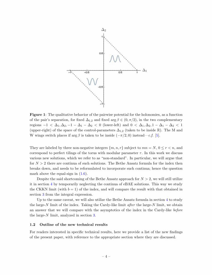
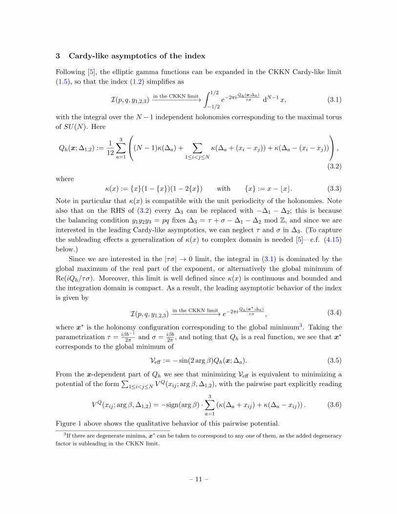
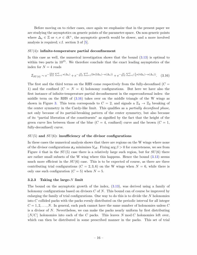
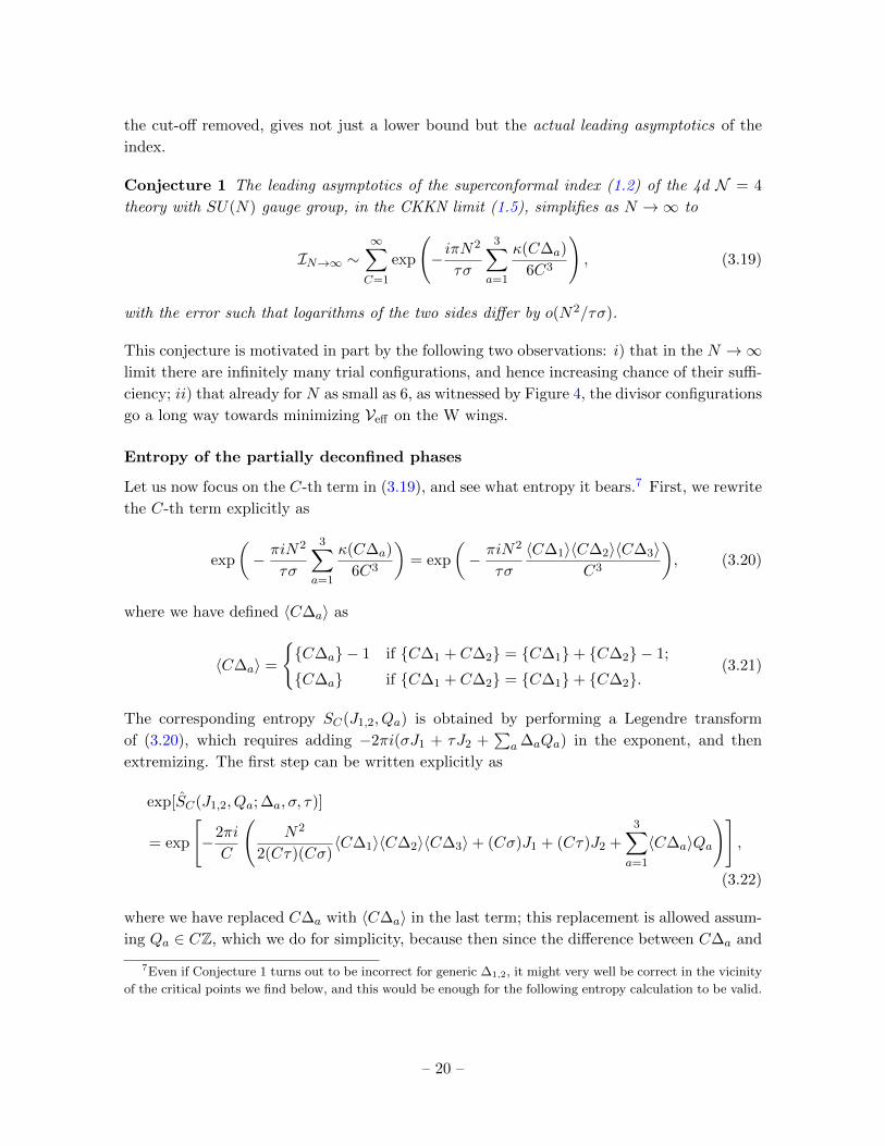

02 04 06 08 10Re (u)
002
004
006
008
010
Im(u)
(a) (∆1∆2) = (105517
75287 )
02 04 06 08 10Re (u)
002
004
006
008
010
Im(u)
(b) (∆1∆2) = ( 75287
152517 )
Figure 5 Numerical solutions to the eBAEs (47) with N = 11 and τ = 1+23i230 Note that
(a) corresponds to Case 1 (∆1 + ∆2 le 12) and (b) corresponds to Case 2 (∆1 + ∆2 gt
12)
to both packs having holonomies equally spaced along the periodic τ direction and hence
can be viewed as a natural odd-N version of the standard C = 2 solution Although this
solution only satisfies the eBAEs asymptotically we have demonstrated that similar solutions
continue to exist at finite τ by numerically solving the exact eBAEs (47) As an example
we present a numerical solution with N = 11 in Figure 5a This strongly implies that there
is an exact non-standard solution to the eBAEs (47) whose asymptotic form is given as
(419) Unlike the standard solutions however this non-standard C = 2 solution does not
have the holonomies uniformly distributed on the torus and moreover generally depends on
the potentials ∆a except in the Cardy-like limit
It is now straightforward to insert the asymptotic solution (419) into (416) to obtain
the contribution to the index
log Iodd-NC=2 (∆a τ) = minus πi
6τ2
3suma=1
N2 minus 1
8κ(2∆a) +O (1τ) (420)
which can be compared with the standard C = 2 solution
log Ieven-NC=2 (∆a τ) = minus πi
6τ2
3suma=1
(N2
8κ(2∆a)minus κ(∆a)
)+O (1τ) (421)
obtained by taking C = 2 in (417) Although these expressions still demonstrate an evenodd
effect at finite N the leading O(N2τ2) behavior is identical in the large-N limit
Case 2 ∆1 + ∆2 gt12
We now turn to the second possibility where the chemical potentials satisfy ∆1 + ∆2 gt12
Here the non-standard solution takes the asymptotic form
u =
plusmn∆1 minus ε
2
cup
i
(N minus 3)2τ i = 0 middot middot middot N minus 5
2
cup
1
2+
iminus 12
(N minus 1)2τ i = 1 middot middot middot N minus 1
2
(422)
ndash 27 ndash
This corresponds to two isolated holonomies along with packs of (N minus 3)2 and (N minus 1)2
holonomies respectively Numerically we can see that for sufficiently large τ the first two
holonomies are actually part of a single pack of (N + 1)2 holonomies just as in case 1
However as Im τ approaches zero this pair first moves towards the real axis and then finally
towards plusmn∆12 in the Cardy-like limit The exponentially small deviation ε away from this
endpoint is given by
ε =τ
2πiexp
[minusπiτ
(minusN minus 1
2+ (N minus 2)∆1 + (N minus 1)∆2
)] (423)
provided the quantity in the parentheses is positive This is true for a generic value of
∆1 + ∆2 gt12 (not asymptotically close to 1
2) and a sufficiently large N Although (422) only
holds asymptotically numerical solutions of this type can be obtained for finite τ and we
provide an example in Figure 5b
Inserting the non-standard solution (422) into the asymptotic expression (416) then
gives the contribution to the index
log Iodd-NC=2 (∆a τ) = minus πi
6τ2
[3sum
a=1
N2
8κ(2∆a) +
3N
2(1minus 2∆2)(1minus 2∆3)
+3
4minus 3∆2 + 3(∆1 + ∆2)(minus2∆1 + ∆2 + 2∆1∆2)
]+O (1τ)
(424)
Although this expression is more complicated than the corresponding one for Case 1 it reduces
in the large-N limit to the same leading order behavior as all the other C = 2 cases namely
log IC(∆a τ) = minusπiN2
τ2
3suma=1
κ(C∆a)
6C3+O(N logN 1|τ |) (425)
with C = 2
While we have focused on non-standard solutions for C = 2 numerical investigations
confirm that similar non-standard solutions exist for arbitrary values of C and N at least for
N sufficiently large so that it can be divided into nearly equal packs of holonomies These
non-standard solutions are similar to that with C = 2 in that they are sensitive to the choice
of chemical potentials ∆1 and ∆2 with the simpler configuration corresponding to Case 1
above occurring only when ∆1 + ∆2 le 1C In this case the non-standard solution in the
Cardy-like limit is given by
u =
I
C+
i
(N + C minusD)Cτ I = 0 middot middot middot D minus 1 i = 0 middot middot middot N minusD
C
cupJ
C+
j minus 12
(N minusD)2τ J = D middot middot middot C minus 1 j = 1 middot middot middot N minusD
C
(426)
where N = CbNCc + D (D = 1 middot middot middot C minus 1) This satisfies the eBAEs in the Cardy-like
limit (as displayed in (C22)) up to exponentially suppressed terms In principle this solution
ndash 28 ndash
can be inserted into (416) to obtain the contribution of a given C non-standard solution to
the index The resulting expressions simplify in the large-N limit and reduce to (425) as
expected
Although this extension of the Case 1 solution to arbitrary values of C only holds for
sufficiently small ∆1 + ∆2 we expect that generalizations of the Case 2 solution (where pairs
of holonomies may be pulled away from the main packs) exist for other values of the chemical
potentials We thus conjecture that at least in the Cardy-like limit solutions to the eBAEs
exist for all values of C and N with d le NC lt d+ 1 Here d corresponds to the minimum
number of holonomies in a single pack that allows the solution to be categorized as a set
of packs instead of individually distributed holonomies When C divides N the solution is
standard but otherwise it is non-standard For each value of C the contribution to the index
then takes the form (425) regardless of whether the solution is standard or non-standard
As a result the Bethe-ansatz type approach to the index reproduces the improved asymptotic
bound (317) found above
43 Additional non-standard solutions
As we have seen explicitly the non-standard solutions (419) and (422) to the eBAEs (47) for
C = 2 and odd N contribute to the index in much the same way as the standard 2 N2 0solution for even N at least in the large-N limit Moreover such contributions were crucial
to reproduce the improved asymptotic bounds (317) with arbitrary integer C that may or
may not divide N This makes us conclude that we cannot ignore the non-standard solutions
in the Bethe ansatz approach to the index
While we have focused on non-standard solutions that are similar to the CNC 0solutions since all standard solutions reduce to this form in the Cardy-like limit we have
also found numerical evidence for the existence of non-standard solutions at finite τ This
suggests that many if not all standard mn r solutions have generalized counterparts as
non-standard solutions In addition there may be additional non-standard solutions that do
not fall into any particular classification Thus it would be nice to understand the full set of
solutions to the eBAEs
In principle we would just solve the eBAEs (47) to obtain a complete set of standard
and non-standard solutions However in practice this is a rather challenging problem even
in the asymptotic limits Therefore to make the problem tractable we focus on the N = 2
and N = 3 cases Even so much of the analysis is rather technical so we relegate the details
to Appendix C and only highlight the main results here
431 Non-standard solutions for N = 2
Since the eBAEs (47) depend only on the difference uij = ui minus uj of the holonomies and
since the free parameter λ is unconstrained the N = 2 eBAEs reduce to a single equation for
a single variable u21
1 =3prod
a=1
θ1(∆a + u21 τ)2
θ1(∆a minus u21 τ)2 (427)
ndash 29 ndash
Here for convenience we have used the real chemical potentials ∆123 which are essentially
the same as ∆1∆2minus∆1 minus∆2 up to simple shifts and reflections such that
0 lt ∆a lt 1
3suma=1
∆a = 1 (428)
See Appendix C for more details
Since each theta function has a first-order zero this fraction has six zeros Furthermore
since it is elliptic the fraction takes all values including unity six times and thus the eBAE
has six solutions Four of them are the familiar ones
u21 =
0
1
2τ
2
1 + τ
2
(429)
corresponding to the trivial solution and standard 2 1 0 1 2 0 and 1 2 1 solutions
respectively The other two solutions are non-standard and since the equation is symmetric
under u21 rarr minusu21 they are negatives of each other
u21 = u∆ minusu∆ (non-standard) (430)
It seems challenging to find u∆ in closed form except in the asymptotic limits so part of the
investigation will be numerical
We denote the lsquolow-temperaturersquo limit to be |τ | 1 and the lsquohigh-temperaturersquo limit to
be |τ | 1 where arg τ (6= 0 π) is held fixed for both cases In either limit the Jacobi theta
function θ1(u τ) has a straightforward asymptotic expansion so the equation (427) can be
directly solved The asymptotic analysis is presented in Appendix C and we summarize the
N = 2 results here
As indicated above the standard solutions (429) are exact solutions for any ∆a and for
all τ so we only focus on the non-standard solution specified by u∆ In the low-temperature
limit the solutionmdashgiven in (C11)mdashtakes the form
u∆(Im τ rarrinfin) =1
2πilog
minus(1minussum
a cos 2π∆a
2
)+
radicradicradicradic(1minussum
a cos 2π∆a
2
)2
minus 1
(431)
The high-temperature asymptotic solution splits into two cases depending on whether ∆3
is less than or greater than 12 The solution is given by (C26) and (C30) which can be
summarized as
u∆(Im τ rarr 0) =
1
2+τ
4 ∆3 lt
1
2
1minus ∆3 + ilog 2
2πτ ∆3 ge
1
2
(432)
There does not appear to be a simple analytic solution away from these asymptotic limits
However numerical investigations demonstrate that the non-standard solutions (431) and
ndash 30 ndash
Figure 6 Numerical plots of the non-standard N = 2 solution u∆ with arg(τ) = π4 The
figure on the left corresponds to ∆3 lt 12 while that on the right corresponds to ∆3 gt 12
Note that the vertical axis is given in units of (complex) τ
(432) are indeed continuously connected Figure 6 shows explicit examples of the numerical
solution for u∆ with both possibilities of ∆3
To be complete it should be noted that for ∆3 ge 12 the high-temperature limit also
admits a continuous set of solutions
u∆(Im τ rarr 0) =
x+ y τ
∣∣∣∣x isin (1minus ∆3 ∆3) y isin [0 1) and ∆3 ge 12
(433)
which interestingly correspond to the plateaus of Qh in the integral approach of the previous
section However these solutions do not appear to be continuously connected to any solutions
away from the high-temperature limit so we believe they are only an artifact of the high-
temperature asymptotics and are not true solutions to the eBAEs once subleading terms are
included
432 Non-standard solutions for finite N gt 2
The structure of the eBAEs is considerably harder to analyze for N gt 2 as there are more
holonomy pairs uij to consider For any N note that the product of the N individual eBAEs
(47) gives the condition e2πiNλ = 1 so that e2πiλ is a root of unity (not necessarily primitive)
Focusing next on a single equation say i = 1 then gives the condition
1 =
3proda=1
Nprodj=2
(θ1(∆a + uj1 τ)
θ1(∆a minus uj1 τ)
)N (434)
For N = 3 this means we can solve for u31 in terms of u21
3proda=1
θ1(∆a + u31 τ)
θ1(∆a minus u31 τ)= ωk
3proda=1
θ1(∆a minus u21 τ)
θ1(∆a + u21 τ) (435)
where ω = e2πi3 is a primitive cube root of unity and k = 0 1 2 We thus look for non-
standard solutions by picking a given u21 and then (numerically) solving for u31 There are
ndash 31 ndash
three solutions up to periodicity for each value of k giving nine possible roots u31 for a fixed
u21 However not all of these solutions are valid as they must solve not just the i = 1 but
all of the eBAEs Numerically we find in addition to the standard solutions which only exist
at discrete values of u21 that two roots of (435) with k = 0 in fact solve the complete set of
eBAEs for arbitrary u21 (The third k = 0 root is the trivial solution u31 = minusu21 but it does
not generically solve the remaining eBAEs apart from the standard solutions)
Although we only obtain solutions numerically for intermediate values of τ analytic
results are possible in the low and high temperature limits In the low-temperature limit
we take the two independent holonomies to be u21 and u31 and write z21 = e2πiu21 and
z31 = e2πiu31 The non-standard solutions then correspond to the two roots of the quadratic
expression (C16) which we repeat here for convenience
(1 + z21 + z31)
(1 +
1
z21+
1
z31
)= 3 + 2
suma
cos 2π∆a (436)
The two roots are related by the map uij rarr minusuij corresponding to taking zij rarr 1zij
The important feature of this solution is that the eBAEs reduce to a single condition on
two complex holonomies As a result we end up with a continuous family of non-standard
solutions
To further explore the nature of the non-standard solutions we consider for simplicity
the case where all the chemical potentials are identical to each other namely ∆a = 13 In
this case the right-hand side of (436) vanishes and we find simply
1 + z21 + z31 = 0 or 1 +1
z21+
1
z31= 0 (437)
Since the second case can be obtained from the first by taking ui rarr minusui we focus on the
first case The expression 1 + z21 + z31 = 0 has a simple interpretation in the complex plane
as a triangle with sides 1 z21 and z31 Since the solution is restricted to |q| le |z21| le 1 and
|q| le |z31| le 1 the space of solutions is given by the intersection of two disks of radius one
centered at 0 and 1 respectively The continuous family of non-standard N = 3 solutions is
shown schematically in Figure 7
The analysis of the high-temperature asymptotic solutions is rather involved so we again
focus on the case ∆a = 13 In addition to the standard solutions the continuous family
of non-standard solutions survives in the high temperature limit and is given by (C34) in
Appendix C which we rewrite in terms of u21 = x21 + y21τ and u31 = x31 + y31τ
u21 u32 isinu21 u32
∣∣∣∣0 le x21 mod 1 lt 13 u21 minus 2u31 = Z + 1
3τ(Z + 12)
cupu21 u32
∣∣∣∣13 lt x21 mod 1 lt 23 u21 + u31 = Z + 1
3τ(Z + 12)
cupu21 u32
∣∣∣∣13 lt x21 mod 1 lt 23 2u21 minus u31 = Z + 1
3τ(Z + 12)
cupu21 u32
∣∣∣∣23 lt x21 mod 1 lt 1 u21 minus 2u31 = Z + 13τ(Z + 1
2)
(438)
ndash 32 ndash
(a) 1 + z21 + z31 = 0 (b) 1 + 1z21 + 1z31 = 0
Figure 7 The space of non-standard N = 3 solutions in the low-temperature limit with
identical chemical potentials ∆a = 13 Solutions of the first type satisfying 1+z21 +z31 = 0
are shown in (a) while solutions of the second type satisfying 1 + 1z21 + 1z31 = 0 are
shown in (b)
Figure 8 The space of non-standard N = 3 solutions in the high-temperature limit with
identical chemical potentials ∆a = 13 Here we only show the real components x21 and
x31 under the decomposition uij = xij + yijτ The parameter space is actually one-complex
dimensional which would be apparent if we had not suppressed the y21-y31 plane
This indicates that up to discrete shifts there is a one-complex dimensional family of high-
temperature solutions Although the family appears to be split into four branches the first
and last subset in (438) is part of the same branch as shown in Figure 8
We have verified numerically in several examples that the asymptotic low and high tem-
perature solutions are continuously connected with each other This suggests that the con-
ndash 33 ndash
tinuous family of non-standard solutions is in fact generic for any value of τ In general the
parameter space and the relation between u21 and u31 depends on the chemical potentials
∆a However there is an interesting point (up to permutations) in this space of non-standard
solutions with
u21 = 12 u31 = 1
2τ (439)
which is ∆a-independent This is an exact non-standard solution whose validity can be
checked using (48) We were actually led to it via the correspondence of subsection 211
with N = 1lowast theory it corresponds to a Coulomb vacuum of the compactified N = 1lowast theory
with SU(3) gauge group listed in Doreyrsquos paper [25] as the ldquofifthrdquo vacuum
Despite its simple form somewhat reminiscent of the standard solutions the solution
(439) is part of the continuous family and not isolated To see this we look for vanishing
eigenvalues of the Jacobian matrix (partQipartuj) where the Qi represent the eBAE expressions
as given in (47) In general there are N eBAEs along with N holonomies uj However the
constraintprodiQi = 1 along with the SU(N) constraint
sumj uj isin Z + τZ effectively reduces
this to an (N minus 1)times (N minus 1) matrix
partQipartuj
= minusδijNsumk=1
g(uki ∆a τ) + g(uji ∆a τ)minus g(uNi ∆a τ) (440)
where i j = 1 middot middot middot N minus 1 and we have defined
g(u ∆a τ) equiv3sum
a=1
(θprime1(u+ ∆a τ)
θ1(u+ ∆a τ)+θprime1(minusu+ ∆a τ)
θ1(minusu+ ∆a τ)
) (441)
For the present N = 3 case we find
det
(partQipartuj
)∣∣∣∣(u21u31)=(12τ2)
= 12
(4prod
J=2
3suma=1
θprimeJ(∆a τ)
θJ(∆a τ)
)4sumI=2
1sum3a=1 θ
primeI(∆a τ)θI(∆a τ)
(442)
where θ234 are the standard Jacobi theta functions given explicitly in (B3) We now make
use of the following result
Lemma 2 For any τ in the upper-half plane and any complex ∆123 subject tosum
a ∆a isin Z
we have4sumI=2
1sum3a=1 θ
primeI(∆a τ)θI(∆a τ)
= 0 (443)
This lemma combined with (442) establishes that the Jacobian matrix indeed has a
vanishing eigenvalue This establishes the existence of a ldquozero moderdquo taking (439) to nearby
eBAE solutions Proof10 of this lemma can be found in appendix B
10We are indebted to Hjalmar Rosengren a mathematician at Chalmers University for an instrumental
correspondence regarding the proof
ndash 34 ndash
Although we have yet to perform an analytic investigation of the non-standard solutions
for N gt 3 we have investigated some cases numerically For N = 4 and 5 in addition to
the isolated standard solutions we find solutions on which partQipartuj has a single vanishing
eigenvalue suggesting that they are part of one-complex dimensional families of solutions
More interestingly for N = 6 7 8 and 9 we find evidence for both one and two complex di-
mensional families of solutions the latter signalled by two vanishing eigenvalues for partQipartuj
Similarly for N = 10 we find evidence for one two and three complex dimensional families
of solutions These are in agreement with the expectation that the continuous families of
solutions correspond to Coulomb vacua of N = 1lowast theory Based on these numerical results
and the putative correspondence with N = 1lowast theory we conjecture that at least the dimen-
sionality of the space of the N = 4 eBAE solutions is captured correctly by the semi-classical
formula for the rank of the Coulomb vacua in SU(N) N = 1lowast theory
Conjecture 2 For N ge (l+1)(l+2)2 generic τ in the upper-half plane and generic ∆12 isinC the SU(N) N = 4 eBAEs in (47) have l-complex-dimensional continua of solutions
The existence of such flat directions is somewhat unusual nevertheless in that it necessar-
ily demands the existence of non-trivial identities among products of Jacobi theta functions
Of particular significance is that the existence of continuous solutions to the eBAEs poses
a serious issue to the full validity of the Bethe ansatz type approach as established in Ref [19]
The reason is that the rewriting of the index (12) into the Bethe ansatz form relies on the
fact that the general solutions to the eBAEs are isolated so that Cauchyrsquos formula may be
applied [19] Hence if there are continuous families of non-standard solutions the Bethe
ansatz type approach must be reformulated to incorporate such continuous Bethe roots into
the sum over solutions to the eBAEs (410)
44 The large-N limit of the index revisited
While we have been motivated by the Cardy-like limit of the index the appearance of partially
deconfined phases as well as non-standard solutions suggests that we re-examine the large-N
limit at finite τ as investigated in Ref [6] In this large-N limit one or at most a few solutions
(if there are any degeneracies) to the BAE would be expected to dominate in the sum over
solutions (410) The focus is then on identifying the dominant solution much as one would
search for a dominant saddle point contribution
The main emphasis in [6] was on the basic solution corresponding to I1N0(∆a τ) In
the large-N limit the contribution was found to be
log I1N0(∆a τ) =
Nminus1sumjjprime=0 (j 6=jprime)
log
prod3a=1 Γ
( jminusjprimeN τ + ∆a τ τ
)Γ( jminusjprimeN τ τ τ
) +O(N logN)
= minusπiN2Θ(∆a τ) +O(N logN) (444)
ndash 35 ndash
where Θ(xa τ) is defined as
Θ(xa τ) equivsum3
a=1 κτ (xa)
6τ2+
3sum3
a=1xaτ (1minus xaτ )minus (1minus τ)(1minus 2τ)
3τminus
3suma=1
(1minus xaτ )
(445)
where xτ and κτ (x) are defined in (415) Using the constraint ∆3 = 2τ minus∆1minus∆2 we can
rewrite Θ(∆a τ) explicitly as
Θ(∆a τ) =
(∆1τminus1)(∆2τminus1)(2τ+1minus∆1τminus∆2τ )
τ2 (∆1 + ∆2τ = ∆1τ + ∆2τ minus 1)∆1τ∆2τ (2τ+1minus∆1τminus∆2τ )
τ2 minus 1 (∆1 + ∆2τ = ∆1τ + ∆2τ )
(446)
and therefore (444) is in fact a function of ∆1 ∆2 and τ only
While it is clear that the basic solution yields a contribution of (N2) there are potentially
many other sources of contributions at the same order These include other standard mn rsolutions as well as isolated and continuous families of non-standard solutions The conjecture
of Ref [6] is that only the set of T -transformed solutions u1Nr would yield additional
contributions at O(N2) The resulting large-N index is then argued to take the form
log I(q q y123) = max
log I1Nr(∆a τ) r isin Z
+O(N logN)
= maxminusπiN2Θ(∆a τ + r) r isin Z
+O(N logN) (447)
unless the ∆arsquos are located along Stokes lines where the asymptotic expansions of the elliptic
functions fail to converge or where different contributions may compete with each other
We note that there is some tension between the conjectured large-N index (447) and
our conjectured leading asymptotics in the CKKN limit namely (319) In particular the
latter as well as the more rigorous bound (317) include configurations where the holonomies
are split into C nearly equal packs distributed evenly on the circle and this is not visible
in (447) Of course it is possible that the Cardy-like limit and the large-N limit do not
commute Nevertheless this motivates us to ask whether additional solutions to the eBAEs
either standard or non-standard may contribute at large N
441 A new parametrization of the standard solutions
In the Cardy-like limit we have seen that standard solutions obtained from C identical packs
of NC collided holonomies will contribute at O(τminus2(N2C3)
) Here we are assuming that C
divides N so this is a standard solution If the limit is smooth then we expect this behavior
to persist even as we move away from the Cardy-like limit As in (413) the standard
mn r solutions that reduce to C packs of holonomies have gcd(n r) = NC This can be
parametrized as the set of standard solutionsC
p pN
C qN
C
C|N p|C and gcd(p q) = 1 (448)
ndash 36 ndash
The set of configurations for a given C all have C packs of holonomies with the packs equally
spaced 1C apart on the periodic unit circle The NC holonomies within each pack are
equally spaced (CN)τ apart on the periodic τ cycle To obtain a periodic tiling of T 2 each
subsequent pack is offset by (sN)τ from the previous one where s = 0 1 C minus 1 so there
are precisely C distinct standard solutions in the set of configurations for a given C In
fact this classification of standard solutions by the number of packs C allows for a new (but
equivalent) parametrization of the standard solutions (49) labeled now by
C s where C|N and s = 0 1 C minus 1 (449)
For a given C s the holonomies solving the eBAEs are
uCs =
uab = u+
a
C+bC + as
Nτ
∣∣∣∣C|N 0 le s lt C (a b) isin ZC times ZNC
(450)
Here a labels the pack and b labels a particular holonomy within that pack
In the large-N limit provided C sim O(1) the holonomies become dense along the τ
circle and hence the shift between packs by a fraction sN does not qualitatively change the
appearance of the solution This suggests that we can compute ICs in the large-N limit in a
universal manner provided C sim O(1) so that NC remains large To do so we start with the
expression for the standard solution given in (411) Ignoring the subleading contributions
from the prefactor αN (τ) and the Jacobian H(uCs ∆a τ)minus1 as in [6] then gives
log ICs(∆a τ)
=
Cminus1sumprime
aaprime=0
NCminus1sumprime
bbprime=0
log
prod3a=1 Γ
((aminus aprime)( 1
C + τNs) + bminusbprime
NC τ + ∆a τ τ)
Γ((aminus aprime)( 1
C + τNs) + bminusbprime
NC τ τ τ) +O(N logN) (451)
where the primes in the summation symbols indicate that the (a b) = (aprime bprime) case is excluded
This can be rewritten as
log ICs(∆a τ)
= C
NCminus1sumprime
bbprime=0
log
prod3a=1 Γ
(bminusbprimeNC τ + ∆a τ τ
)Γ(bminusbprimeNC τ τ τ
)+
Cminus1suma=1
NCminus1sumbbprime=0
(C minus a) log
prod3a=1 Γ
(bminusbprimeNC τ + a( 1
C + τNs) + ∆a τ τ
)Γ(bminusbprimeNC τ + a( 1
C + τNs) τ τ
)+ a log
prod3a=1 Γ
(bminusbprimeNC τ + (aminus C)( 1
C + τNs) + ∆a τ τ
)Γ(bminusbprimeNC τ + (aminus C)( 1
C + τNs) τ τ
)+O(N logN)
(452)
ndash 37 ndash
where on the first line the b = bprime case is excluded In fact the first line is similar to the
expression (444) for the basic 1 N 0 solution but with N replaced by NC and with an
extra prefactor of C Note that the replacement N rarr NC in the large-N formula is valid
since we have assumed C sim O(1) The second line can be simplified using the formulas (for
∆ 6= 0) [6]
Nminus1sumprime
jjprime=0
log Γ
(j minus jprime
Nτ + ∆ τ τ
)= πiN2 (τ minus ∆τ + 1)(τ minus ∆τ + 12)(τ minus ∆τ )
3τ2+O(N)
(453a)
Nminus1sumprime
jjprime=0
log Γ
(j minus jprime
Nτ τ τ
)= πiN2 τ(τ minus 12)(τ minus 1)
3τ2+O(N logN) (453b)
along with (444) The result is
log ICs(∆a τ) = minusπiN2
C
(Cminus1suma=0
Θ(∆a +a
C τ)minus (C minus 1)(C(1minus 3τ) + 1)
6Cτ
)+O(N logN) (454)
provided that ∆a is not an integer multiple of 1C In particular this demonstrates O(N2)
scaling of the standard C s solution for C sim O(1) even away from the the Cardy-like
limit Moreover this leading-order behavior is independent of the offset s along the τ circle
between adjacent packs of holonomies thus confirming the intuition that once the packs are
sufficiently dense the distribution of holonomies within each pack becomes unimportant at
least at leading order
The analysis of the large-N limit of the standard solutions is still incomplete as we have
not considered the case where C scales with N Nevertheless the contributions (454) suggests
that the conjecture (447) must be refined by enlarging the holonomy configurations that need
to be considered In terms of the C s labels the basic 1 N 0 solution is included as 1 0while the T-transformed 1 N r solutions fall under C s with r = qNC where q and C
are relatively prime Note that this presents a bit of a puzzle as (454) and (447) appear to
be in conflict except for r = 0
The resolution of this puzzle is based on two observations The first is that for r sim O(1)
in the large-N limit we must have C sim N in which case the expression (454) breaks down
The second is that if instead C sim O(1) then r must be large However in this case the
map from the first to the second line of (447) breaks down as it is only valid for r scaling as
O(N0) This is because the derivation of Θ(∆a τ + r) from the large-N asymptotics of the
standard solution (411) with mn r = 1 N r was based on making the shift τ rarr τ + r
However shifts with r = O(N) may lead to a modification to log I1Nr(∆a τ) that is not
captured by simply shifting τ in (444)
Provided we only take standard solutions into account the large-N limit of the index
will be given by maximizing over all C s solutions Although we are unable to provide an
ndash 38 ndash
analytic expression for C sim O(N) we nevertheless expect the large-N index to take a form
along the rough lines of
log I(q q y123) = maxCsimO(1)rsimO(1)
minusπiN
2
C
Cminus1sumj=0
Θ(∆a +j
C τ + r)minus (C minus 1)(C(1minus 3(τ + r)) + 1)
6C(τ + r)
+O(N logN) (455)
where C divides N for standard solutions The shift of τ rarr τ + r in the above allows us to
include T-transformed versions of the C s solutions and the restriction of this expression
to C = 1 reproduces the conjecture (447) of [6]
Of course this is still expected to be incomplete as we have not yet accounted for the non-
standard solutions We know from the Cardy-like limit that isolated non-standard solutions
exist for all integer values of C Numerically these solutions are continuously connected to low
temperature solutions and hence should exist for arbitrary τ Again in the large-N limit
the isolated non-standard solutions correspond to C packs of either bNCc or bNCc + 1
holonomies distributed along the τ circle Since we take C sim O(1) the difference between
packs shows up as a O(1N) correction and hence we expect the leading O(N2) behavior to
be correctly captured by (455) where we now drop the restriction that C divides N
Finally we are able to connect the large-N limit of the index (455) to the Cardy-like
limit by taking τ rarr 0 Looking only at the leading O(1τ2) order it is easy to see that all
terms with r 6= 0 will not contribute Making use of
Θ(∆a τ) =1
6τ2
3suma=1
κτ (∆a) +O(1|τ |) (456)
along with the identity (312) then gives
log I(q q y123) = maxCsimO(1)
minusπiN
2
τ2
3suma=1
κτ (C∆a)
6C3
+O(N logN 1|τ |) (457)
in perfect agreement with the conjecture (319) for the leading large-N asymptotics in the
Cardy-like limit This certainly suggests that the asymptotic behavior of the index is inde-
pendent of the order of limits between the Cardy-like limit and the large-N limit Of course
in order to remove the conjectures and be more rigorous in the Bethe Ansatz approach we
have to consider solutions with C sim O(N) as well as the issue of continuous non-standard
solutions
5 Discussion
51 Summary and relation to previous work
Several papers investigating asymptotic growth of supersymmetric indices of the 4d N = 4
theory have appeared in the last year Below we outline how our findings complement those
of the most closely related recent work
ndash 39 ndash
bull Cardy-like asymptotics of the N = 4 index Choi-Kim-Kim-Nahmgoong (CKKN)
[3] Honda [4] and Ardehali [5] All three of these papers investigated the Cardy-like
limit of the 4d N = 4 index I(p q yk) using its integral representation and in the limit
where yk approach the unit circle (for yk not approaching the unit circle the problem
is still openmdashsee Problem 2 in [5] and subsection 52 below) CKKN [3] took actually
also a large-N limitmdashafter the Cardy-like limitmdashto simplify the analysis but in [4 5]
N was left arbitrary CKKN [3] assumed that the dominant holonomy configurations
in the Cardy-like limit correspond to equal holonomies xij = 0 it was later realized in
[4 5] that this assumption fails in essentially half of the parameter-space (see the Added
Note of [5] for the relation between the findings of [4] and [5]) As in [5] we divide the
parameter-space into complementary M wings and W wings While on the M wings the
dominant holonomy configurations indeed correspond to xij = 0 and the asymptotics
has been understood on the W wings finding the Cardy-like asymptotics has been an
open problemmdashsee Problem 1 of [5] In section 3 we solved this problem for N le 4 and
also conjectured the formula (319) in the large-N limit In particular for N = 4 as
well as in the large-N limit we have discovered regions on the W wings corresponding
to partially deconfined phases in the Cardy-like limit of the 4d N = 4 index
bull Large-N asymptotics of the N = 4 index Benini-Milan [6] This reference studied
the large-N limit of the 4d N = 4 index using its Bethe Ansatz representation In the
present paper we pointed out some difficulties with the Bethe Ansatz representation for
N ge 3 there seem to be continuous families of Bethe roots calling for an integration
measure which is so far not understood Setting this difficulty aside we pointed out
that some of the discrete Bethe roots (found in [20]) are not negligible in the large-N
limit of the index as assumed in [6] We moreover discovered new discrete Bethe roots
that play an important role in the large-N asymptotics of the index The new non-
negligible contributions that we have found demonstrate partially deconfined phases in
the large-N limit of the index as well
bull Large-N asymptotics of the N = 4 index via the density-distribution ap-
proach CKKN [7] In this reference following the original work of Kinney-Maldacena-
Minwalla-Raju [2] the large-N limit of the index was analyzed using its integral rep-
resentation by rewriting the integral in terms of ρn =sumN
j=1 e2πinxj rather than xj
These new variables are Fourier coefficients of the density distribution ρ(x) for the
holonomies in the large-N limit The drawback of this approach is that the range of
ρn does not appear to be simple to derive This difficulty hinders an accurate analysis
of the saddle-points of the integral over the ρn variables We have thus avoided this
approach in the present work
bull Cardy-like asymptotics of the N = 1 index on higher Riemann sheets Kim-
Kim-Song [27] and Cabo Bizet-Cassani-Martelli-Murthy [28] Since the fugacities of
the index satisfy y1y2y3 = pq one can ldquoturn off the flavor fugacitiesrdquo by setting yk =
ndash 40 ndash
(pq)13 the resulting function I(p q (pq)13) is the usual N = 1 superconformal index
of the N = 4 theory and is known not to have fast asymptotic growth in the usual
Cardy-like limit p q rarr 1 due to bose-fermi cancelations [More precisely for SU(N)
N = 4 theory it can be shown from the results in [23] that I(p q (pq)13) grows like
βNminus1 not like e1β2as expected from the bulk black holes [15]] These statements
are not the end of the story however as they really apply only to the fundamental
Riemann sheet of the function For p q inside the unit open punctured disc the function
I(p q (pq)13) unlike the more well-behaved I(p q yk) is not meromorphic therefore
besides turning on flavor fugacities there is another way to get fast growth from itmdash
or ldquoobstruct its bose-fermi cancelationsrdquo if you willmdashand that is to go to its higher
Riemann sheets Because of the power 13 for pq the non-meromorphic N = 1 index
I(p q (pq)13) has in fact three inequivalent sheets which can be identified along branch
cuts at arg p = π and be labeled by n0 = minus1 0+1 The papers [27 28] show that
on the n0 = plusmn1 sheets it is possible to get the fast exponential growth associated to
the bulk black holesmdashsimply note that p rarr pe2πin0 introduces nontrivial phases in
(pq)13 equivalent to ldquoturning on flavor fugacitiesrdquo and setting yk = (pq)13e2πin03
on the n0 = 0 sheet corresponding to ∆a = n03 in the CKKN limit which can
obstruct the bose-fermi cancelations as familiar from CKKNrsquos work [3] Now while for
sign(arg β) = plusmn the Cardy-like asymptotics of the index has been obtained from the
fully-deconfining holonomy configurations on the n0 = plusmn1 sheets on the other (n0 =
∓1) sheets we expect that the partially deconfined configurations become significant
Note that here the control-parameters are n0 sign(arg β) In particular for the SU(4)
N = 4 theory it follows from our results in section 3 that it is the partially-deconfining
Z4 rarr Z2 holonomy configurations which take over on the n0 = ∓1 sheets Similarly
if our conjecture (319) is correct in the large-N limit the partially-deconfining ZN rarrZN2 holonomy configurations take over on the n0 = ∓1 sheets (As discussed in
subsection 323 when N is odd as N rarr infin we can approximate the problem by
replacing N rarr N minus 1 and then consider the ZNminus1 rarr Z(Nminus1)2 configurations instead)
The results of [27 28] also imply universal expressions for the asymptotics of the N = 1
indices of large classes of 4d SCFTs on parts of their n0 = plusmn1 sheets We expect
that on other parts of those sheets as well as on other sheets when available partially
deconfined phases with different asymptotics might arise
bull Higher Riemann sheets of the N = 1 index with path-integration Cabo Bizet-
Cassani-Martelli-Murthy [43] This reference is also related to analytic continuation of
the N = 1 index to the n0 6= 0 sheets and is in fact the pioneering work on investiga-
tion of such higher sheets However it adopts a Lagrangian (path-integral) approach
whose analytic continuation is not properly understood In particular the path-integral
computation in [43] suffers from subtleties regarding regularization of the analytically
continued supersymmetric Casimir energy as discussed in footnote 13 of [43] already
before analytic continuation the regularization scheme used there does not give the cor-
ndash 41 ndash
rect result when applied to general theories and it is somewhat of a coincidence that
it works for the N = 4 theory There seems to be no reason to believe that the scheme
keeps being coincidentally correct in the analytically continued case which is relevant
to black hole counting [Such subtleties can be overcome when working with the path-
integral version of the N = 4 index I(p q yk) in the CKKN limit though which would
be relevant to the analysis here see section 4 of [5] where this issue was addressed]
bull Large-N asymptotics of the N = 1 index on higher Riemann sheets Cabo Bizet-
Murthy [45] This paper studies the large-N asymptotics of the N = 1 index (with
p = q) of the N = 4 theory on its n0 6= 0 sheets in the density-distribution approach
It adopts a variational perspective and looks for saddle-point configurations of ρ(x)
instead of working with the subtle Fourier coefficients ρn While the focus of [45] is on
the saddle-point configurations corresponding to the standard mn r eBAE solutions
with gcd(mn r) = 1 our results imply that detecting the partially deconfined phases
in their approach requires investigating more general saddle-point configurations corre-
sponding to the standard eBAE solutions with gcd(mn r) gt 1 as well as configurations
corresponding to non-standard eBAE solutions
bull The topologically-twisted N = 4 index Hosseini-Nedelin-Zaffaroni [44] and Hong-
Liu [20] Besides the superconformal index there is the rich and interesting topologically-
twisted index that one can compute exactly for the N = 4 theory This index has been
analyzed using a Bethe Ansatz expression with precisely the same eBAEs that feature
in the 4d N = 4 superconformal index Our results in this paper thus imply that the
expressions analyzed in [44] and [20] too for rank ge 2 suffer from the difficulty of
continuously connected Bethe roots Furthermore in some regions of the parameter-
space this index exhibits a well-understood fast asymptotic growth of type e1β in the
Cardy-like limit which is associated to black strings in AdS5 [44] In the rest of the
parameter-space finding the asymptotics is more challenging however [20] In those
regions we expect that the new discrete solutions that we introduced in this paper are
of significance in the Cardy-like asymptotics of the topologically twisted index
52 Future directions
We conclude by outlining some of the interesting open problems and exciting prospects related
to this work
bull The Bethe Ansatz approach There are several important open questions regarding
the Bethe Ansatz approach Already at rank 1 (ie for SU(2)) where the Bethe Ansatz
formula seems valid not all the solutions of the eBAE are known as discussed in
section 4 besides the four standard solutions [20] 0 12 τ2 (1 + τ)2 there are two
more solutions of the form plusmnu∆ and it would be nice to find u∆ in closed form
For rank ge 2 we have given numerical evidence that there is a continuously connected set
of solutions undermining the Bethe Ansatz formula in its current form as a finite sum
ndash 42 ndash
over eBAE vacua it would be nice to have a proof for existence of uncountably many
Bethe roots for rank ge 2 It would also be important to find ways of reformulating the
BA approach to incorporate the continuous sets of Bethe roots into account It would
moreover be necessary for black hole-counting applications (as in [6]) to characterize
all the Bethe roots contributing to the leading asymptotics of the index in the large-N
limit (We expect similar challenges facing the analyses in [46 47] as well)
bull General Cardy-like asymptotics and black holes with unequal charges As
remarked above the Cardy-like asymptotics of the 4d N = 4 index for general complex
∆12 is still an open problem This problem is relevant to the microstate counting of
the bulk black holes with unequal charges because it is only for the equal-charge black
holes that ∆12 isin R as we have assumed [5] While it might be quite challenging to
address this problem for arbitrary N in the SU(2) case this does not seem out of reach
finding the asymptotic form of u∆ would lead to the desired asymptotics using the Bethe
Ansatz formula
bull The gravity dual of the partially deconfined phases The bulk duals of the
partially-deconfined phases have not been constructed as far as we are aware They
should be new black objects and their accurate interpretation is not clear to us at
this point It is tempting to speculate that they correspond to multi-center black holes
which in cases with lens-space horizon topology are sometimes referred to as black lenses
[48 49] (We expect partially-deconfined phases in the indices analyzed in [46 47 50]
as well with new possibly multi-center black objects associated to them in the bulk)
bull The black hole operators One of the most exciting aspects of the recent advances
in AdS5CFT4 microstate counting is the prospect they open for explicit construction
of the operators dual to the bulk BPS black holes The operators dual to the bulk
KK multi-particle states have long been known of course they are the multi-trace op-
erators generated by the famous single-trace operators nicely reviewed in Table 7 of
[51] for instance The black hole operators on the other hand have been elusive even
in AdS3CFT2 We hope that the emerging refined understanding of the asymptotic
growth of the 4d N = 4 index can guide future pursuits of these long-sought operators
in the N = 4 theory
Note added After the first version of the present paper appeared on arXiv we became aware
that the latest version of [28] contains the contribution of a divisor holonomy configuration to
the Cardy-like asymptotics of the N = 1 index on its higher Riemann sheets In particular
Eq (350) in that work is essentially the analog of our (313) in that context Our conjecture
(319) suggests that in the large-N limit at least for the N = 4 theory (and presumably also
in various other holographic SCFTs) irrespective of whether N is even or odd Eq (350) of
[28] with K = 2 would give the leading Cardy-like asymptotics in parameter-regimes (such
as Re(iτσ) gt 0 n0 = minus1) which were previously unexplored
ndash 43 ndash
Acknowledgments
We thank F Benini D Cassani T Hansen Y Lu R de Mello Koch and J Minahan
for related discussions D Speyer for correspondence on Lemma 1 and H Rosengren for
correspondence on Lemma 2 AAA would like to thank P Milan for suggesting numerical
investigation of the Cardy-like limit JTL wishes to thank B Willett for raising the issue
of non-standard solutions to the eBAEs This work was supported in part by the Knut and
Alice Wallenberg Foundation under grant Dnr KAW 20150083 and by the US Department
of Energy under grant DE-SC0007859 JH is supported in part by a Leinweber Graduate
Fellowship from the University of Michigan
A Proof of Lemma 1
Cover the torus R2Z2 with balls of radius ε2 By the pigeonhole principle there are
two integers A lt B such that (Ax Ay) and (Bx By) are in the same ball Then
((B minusA)x (B minusA)y) is in the ball of radius ε around 0 (mod Z2)
Now if (B minusA)x+ (B minusA)y gt 1 we are done by taking C = B minusA
If on the other hand (B minusA)x+ (B minusA)y lt 1 then the relation
αminus β =
α minus β α ge βα minus β+ 1 α lt β
(A1)
guarantees that for ε small enough we have ((B minus A minus 1)x + (B minus A minus 1)y) gt 1 so we
are done by taking C = B minusAminus 1 QED
Let us see how things work in an example Take x = y = 13 The two values B = 6 and
A = 3 are acceptable Now since (BminusA)x+(BminusA)y = 1+1 = 0 lt 1 we can take
C = B minus Aminus 1 = 2 Indeed 2 middot 13+ 2 middot 1
3 = 43 gt 1 as desired As explained above (318)
this implies that for arg β lt 0 at the point (∆1∆2) = (13 13) the bound in (318) with
C = 2 guarantees a partially deconfined behavior for INrarrinfin
B Proof of Lemma 2
Using the identity
θprime1(n τ) = θ2(n τ)θ3(n τ)θ4(n τ) (B1)
for an arbitrary integer n isin Z we can generalize Theorem 21 of [52] as
3suma=1
θprimeI(∆a τ)
θI(∆a τ)=
+θprime1(nτ)θI(nτ)
prod3a=1
θ1(∆aτ)
θI(∆aτ)(I = 3)
minus θprime1(nτ)θI(nτ)
prod3a=1
θ1(∆aτ)
θI(∆aτ)(I = 2 4)
(B2)
ndash 44 ndash
wheresum
a ∆a = n isin Z Here θ234 are related to θ1(u τ) defined in (46) via
θ2(u τ) = θ1(u+ 12 τ) (B3a)
θ3(u τ) = eπiτ4 eπiuθ1(u+ (1 + τ)2 τ) (B3b)
θ4(u τ) = minusieπiτ4 eπiuθ1(u+ τ2 τ) (B3c)
These theta functions are basically obtained from θ1(u τ) by shifting the first argument u by
three different half-periods 12
1+τ2 τ2 respectively They satisfy the so-called Jacobirsquos formula
together with θ1(u τ) namely [53]
2θ1(u0 u1 u2 u3 τ) = θ1(uprime0 uprime1 uprime2 uprime3 τ) + θ2(uprime0 u
prime1 uprime2 uprime3 τ)
minus θ3(uprime0 uprime1 uprime2 uprime3 τ) + θ4(uprime0 u
prime1 uprime2 uprime3 τ) (B4)
where 2uprimeα =sum3
β=0 uβ minus 2uα (α = 0 1 2 3) and we have used the abbreviations
θI(u0 u1 u2 u3 τ) equiv3prod
α=0
θI(uα τ) (B5)
Since θ1(n τ) = 0 for an arbitrary integer n isin Z the following special case of Jacobirsquos formula
(B4) is valid forsum
a ∆a = n isin Z
0 = θ2(n ∆1 ∆2 ∆3 τ)minus θ3(n ∆1 ∆2 ∆3 τ) + θ4(n ∆1 ∆2 ∆3 τ) (B6)
Combining (B6) and (B2) establishes the lemma QED
As discussed in the main text the lemma proves that the SU(3) eBAEs have a ldquozero
moderdquo at the exact non-standard solution (439)
C The elliptic Bethe Ansatz equations in the asymptotic regions
In this appendix we investigate the eBAEs (47) in the asymptotic regions including both
the low-temperature (|τ | 1) and the high-temperature (|τ | 1) limits Then we look for
asymptotic non-standard solutions for N = 2 and N = 3
Before getting into details first we rewrite (47) as
1 = Qi = e2πiλNprodj=1
3proda=1
θ1(uji + ∆a τ)
θ1(uij + ∆a τ) (C1)
where for notational convenience we have introduced ∆a as
∆a =
∆a (a = 1 2)
minus∆1 minus∆2 (a = 3)(C2)
ndash 45 ndash
This is to avoid using a complex ∆3 = 2τ minus∆1 minus∆2 and to keep all the chemical potentials
∆a real We now use quasi-periodicity and the oddness of θ1(u τ) namely (48) to rearrange
the chemical potentials ∆a and the holonomies uk for convenience when writing down the
asymptotic expansions Note that we always assume ∆12 isin R or equivalently ∆a isin R
We start with shifting ∆a by integers using (48) so that 0 le Re ∆a lt 1 is satisfied This
yieldssum
a ∆a isin 0 1 2 Then since the eBAEs (C1) are invariant under ∆a rarr 1minus ∆a and
λ rarr minusλ due to (48) redefining ∆a as ∆a rarr 1 minus ∆a does not change the eBAE solutions
ui Therefore we can redefine ∆a as ∆a rarr 1minus ∆a wheneversum
a ∆a = 2 and consequently
we havesum
a ∆a isin 0 1 Finally we assume ∆a isin R then 0 le Re∆a lt 1 together withsuma ∆a = 0 leads to ∆a = 0 which is forbidden for the index to converge So we have
0 lt ∆a lt 13sum
a=1
∆a = 1 (C3)
The final expression of ∆a shifted from (C2) is given in terms of ∆a as
∆12 =
∆12 (∆1+ ∆2+ minus∆1 minus∆2 = 1)
1minus ∆12 (∆1+ ∆2+ minus∆1 minus∆2 = 2)
∆3 =
minus∆1 minus∆2 (∆1+ ∆2+ minus∆1 minus∆2 = 1)
1minus minus∆1 minus∆2 (∆1+ ∆2+ minus∆1 minus∆2 = 2)
(C4)
where as usual middot = middot minus bmiddotc and we have assumed ∆12 isin R Z
We can also specify the range of holonomies uk using the same properties of θ1(u τ) given
in (48) The key is that the eBAEs (C1) are invariant under uk rarr uk+pk+qkτ for arbitrary
integers pk qk isin Z Using this invariance we can set uk as
uk = xk + ykτ (0 le xk yk lt 1) (C5)
with yi le yj for i le j without loss of generality
Following the setup (C3) and (C5) now we investigate the eBAEs (C1) in asymptotic
regions and look for non-standard solutions there
C1 Low-temperature asymptotic solutions
We start with the low-temperature (|τ | 1) asymptotic region First we rewrite the infinite
product form of θ1(u τ) (46) as
θ1(u τ) = ieπiτ4 eπi(p+p(p+1)τminusu(2p+1))
infinprodk=1
(1minus e2πikτ )(1minus e2πi((kminus1)τ+(uminusτp)))(1minus e2πi(kτminus(uminusτp)))
(C6)
ndash 46 ndash
where we have defined the integer p as
p =
lfloorImu
|τ | sin θ
rfloor(τ = |τ |eiθ) (C7)
Substituting the form of eBAE solutions uk (C5) and the product form (C6) into the eBAEs
(C1) then gives
eπi(Nminus2λminus1) =3prod
a=1
Nprodj=1
infinprodk=1
(1minus e2πi(minusxij+(kminusyij)τ+∆a))(1minus e2πi(xij+(kminus1+yij)τminus∆a))
(1minus e2πi(xij+(kminus1+yij)τ+∆a))(1minus e2πi(minusxij+(kminusyij)τminus∆a)) (C8)
where the curly bracket denotes mod Z as in (33) Under the low-temperature limit the
contributions from k ge 2 are exponentially suppressed and therefore (C8) reduces to
eπi(Nminus2λminus1) =3prod
a=1
Nprodj=1
(1minus e2πi(xij+yijτminus∆a))(1minus e2πi(minusxij+(1minusyij)τ+∆a))
(1minus e2πi(xij+yijτ+∆a))(1minus e2πi(minusxij+(1minusyij)τminus∆a))times(
1 +O(eminus2π|τ | sin θ))
(C9)
These are the eBAEs reduced under the low-temperature limit which yield Nminus1 independent
algebraic equations They are still involved to solve in general however so we consider simple
cases N = 2 and N = 3
C11 N = 2
For N = 2 the reduced eBAEs (C9) yield a single algebraic equation
plusmn1 =
3proda=1
1minus e2πi(u21minus∆a)
1minus e2πi(u21+∆a)
1minus e2πi(τminusu21+∆a)
1minus e2πi(τminusu21minus∆a)times(
1 +O(eminus2π|τ | sin θ)) (C10)
The complete set of solutions to (C10) is given as
u21 isin
01
2τ
21 + τ
2plusmn 1
2πilog
[minus 1minus
suma cos 2π∆a
2+
radic(1minus
suma cos 2π∆a
2
)2
minus1
] (C11)
Here the first solution is trivial and the next three solutions correspond to the standard
2 1 0 1 2 0 and 1 2 1 solutions respectively The other two low-temperature asymp-
totic solutions are non-standard and completely distinguished from the trivial solution and
the standard mn r-type solutions
C12 N = 3
For N = 3 we define
z21 = e2πiu21 z31 = e2πiu31 ya = e2πi∆a and q = e2πiτ (C12)
Note that the low-temperature limit corresponds to |q| 1 In addition the setup (C5)
restricts
|q| le |z31| le |z21| le 1 (C13)
ndash 47 ndash
Under this restriction the reduced eBAEs (C9) yield two algebraic equations
3proda=1
(1minus yaz21)(1minus yminus1a
qz21
)(1minus yaz31)(1minus yminus1a
qz31
)
(1minus yminus1a z21)(1minus ya q
z21)(1minus yminus1
a z31)(1minus ya qz31
)
=3prod
a=1
(1minus yminus1a z21)(1minus ya q
z21)(1minus ya z31
z21)(1minus yminus1
a q z21z31
)
(1minus yaz21)(1minus yminus1a
qz21
)(1minus yminus1a
z31z21
)(1minus yaq z21z31
)
=3prod
a=1
(1minus yminus1a z31)(1minus ya q
z31)(1minus yminus1
az31z21
)(1minus yaq z21z31
)
(1minus yaz31)(1minus yminus1a
qz31
)(1minus ya z31z21
)(1minus yminus1a q z21
z31) (C14)
up to exponentially small terms of at most O(|q|)If we assume |z31| is strictly greater than |q| then we can simply set q = 0 in (C14) in
the log-temperature limit The resulting equations then simplify and admit a discrete set of
solutions
(z21 z31) = (1 1) cup (ω ωminus1) cup (ωminus1 ω) cup (minus1 0) (C15)
where ω = e2πi3 as well as a continuous family of solutions satisfying a single condition
(1 + z21 + z31)
(1 +
1
z21+
1
z31
)= 3 + 2
suma
cos 2π∆a (C16)
which reduces to the finitely many non-standard solutions for N = 2 given in (C11) under
z31 = z21 Starting with the discrete solutions the first three are based on cube roots of
unity and correspond to the high temperature limit of the standard solutions In particular
the first entry in (C15) corresponds to the C = 1 case and the next two correspond to the
C = 3 cases The final solution in (C15) is novel as it is a non-standard solution that is
nevertheless independent of the chemical potentials ∆a Note that strictly speaking this
solution violates the assumption made above that |z31| gt |q| However it is in fact easy to
see that this extends to an exact non-standard solution
(u21 u31) = (12 τ2) (C17)
for arbitrary τ
Perhaps more interestingly we have found a continuous family of solutions given by
(C16) This one complex dimensional family of solutions is obviously non-standard since it
depends on the chemical potentials ∆a In addition the limiting form of (C16) for z21 rarr minus1
and z31 rarr 0 encompasses the non-standard solution (C17) This suggests that (C17) is not
a discrete solution but rather a part of the continuous family We confirm this explicitly in
Appendix B by demonstrating that the transformation matrix partQipartuj (i j = 1 2) where Qirepresents the i-th BAE contains a zero mode corresponding to a flat direction
C2 High-temperature asymptotic solutions
Next we consider the high-temperature (|τ | 1) asymptotic region Using the infinite
product form of θ1(u τ) in (46) together with the S-transformation
S θ1(uτ minus1τ) = minusiradicminusiτe
πiu2
τ θ1(u τ) (C18)
ndash 48 ndash
we can derive the high-temperature expansion of θ1(u τ)
θ1(u τ) = minusiτeπiτ4 e
πiτu(1minusu)(1minus eminus
2πiτu)infinprodk=1
(1minus eminus2πiτk)(1minus eminus
2πiτ
(kminusu))(1minus eminus2πiτ
(k+u))
= minusiτeπiτ4 (minus1)pe
πiτuτ (1minusuτ )
infinprodk=1
(1minus eminus2πiτk)(1minus eminus
2πiτ
(kminusuτ ))(1minus eminus2πiτ
(kminus1+uτ ))
(C19)
where we have used the notation uτ introduced in (415) and defined the integer p as
p = bReuminus cot θ Imuc (τ = |τ |eiθ) (C20)
Substituting the form of eBAE solutions uk (C5) and the product form (C19) into the eBAEs
(C1) then gives
eπi(Nminus2λminus1) =
3proda=1
Nprodj=1
[eπiτ (minusxij+∆a(1minusminusxij+∆a)minusxij+∆a(1minusxij+∆a))
+ eπi(bminusxij+∆acminusbxij+∆acminus2yij(1minusminusxij+∆aminusxij+∆a))
timesinfinprodk=1
(1minus eminus2πiτ
(kminusminusxij+∆a+yijτ))(1minus eminus2πiτ
(kminus1+minusxij+∆aminusyijτ))
(1minus eminus2πiτ
(kminusxij+∆aminusyijτ))(1minus eminus2πiτ
(kminus1+xij+∆a+yijτ))
]
(C21)
where the curly bracket denotes mod Z as in (33) Under the high-temperature limit the
contributions from k ge 2 are exponentially suppressed and therefore (C21) reduces to
eπi(Nminus2λminus1) =3prod
a=1
Nprodj=1
[eπiτ (minusxij+∆a(1minusminusxij+∆a)minusxij+∆a(1minusxij+∆a))
+ eπi(bminusxij+∆acminusbxij+∆acminus2yij(1minusminusxij+∆aminusxij+∆a))
times (1minus eminus2πiτ
(1minusminusxij+∆a+yijτ))(1minus eminus2πiτ
(minusxij+∆aminusyijτ))
(1minus eminus2πiτ
(1minusxij+∆aminusyijτ))(1minus eminus2πiτ
(xij+∆a+yijτ))
]times(
1 +O(eminus 2π sin θ
|τ | )) (C22)
These are the eBAEs reduced under the high-temperature limit which yieldNminus1 independent
algebraic equations They are still involved to solve in general however so we consider simple
cases N = 2 and N = 3
ndash 49 ndash
C21 N = 2
For N = 2 the reduced eBAEs (C22) yield a single algebraic equation (take logarithmic
function on both sides)
Zπi =πi
τ
3suma=1
(x21 + ∆a(1minus x21 + ∆a)minus minusx21 + ∆a(1minus minusx21 + ∆a))
+ πi3sum
a=1
(bx21 + ∆ac minus bminusx21 + ∆ac+ 2y21(1minus x21 + ∆a minus minusx21 + ∆a))
+
3suma=1
log
[(1minus eminus
2πiτ
(1minusx21+∆aminusy21τ))(1minus eminus2πiτ
(x21+∆a+y21τ))
(1minus eminus2πiτ
(1minusminusx21+∆a+y21τ))(1minus eminus2πiτ
(minusx21+∆aminusy21τ))
]+O(e
minus 2π sin θ|τ | )
(C23)
Solving this equation is quite involved in general mainly because the last logarithmic term
may yield a large contribution for some special values of x21 We therefore solve this equation
under appropriate assumptions on x21
CASE 1 plusmnx21 + ∆a are NOT asymptotically close to 0 or 1
First we consider the solutions where plusmnx21 + ∆a are not asymptotically close to the end
points 0 and 1 In this case the last logarithmic term in (C23) is exponentially suppressed
as sim O(eminus 2π sin θ
|τ | x) where we have defined a real number x isin (0 1) as
x equiv min(x21 + ∆a 1minus x21 + ∆a minusx21 + ∆a 1minus minusx21 + ∆a a = 1 2 3) (C24)
Then (C23) is simplified into the following system of algebraic equations
0 =3sum
a=1
(x21 + ∆a(1minus x21 + ∆a)minus minusx21 + ∆a(1minus minusx21 + ∆a)
) (C25a)
Z =3sum
a=1
(bx21 + ∆ac minus bminusx21 + ∆ac+ 2y21(1minus x21 + ∆a minus minusx21 + ∆a)
) (C25b)
up to O(eminus 2π sin θ
|τ | x) If we set 0 lt ∆1 le ∆2 le ∆3 lt 1 without loss of generality the complete
set of solutions to (C25) can be written as
u21 = x21 + y21τ isin
01
2τ
21 + τ
2
cup
1
2+τ
41
2+
3τ
4
∣∣∣∣∆3 lt1
2
cupx21 + y21τ
∣∣∣∣x21 isin [1minus ∆3 ∆3] y21 isin [0 1) ∆3 ge1
2
(C26)
up to O(eminus 2π sin θ
|τ | x) The complete set of solutions to (C23) corresponding to the CASE
1 is therefore given as (C26) whose subset violating the assumption ldquox21 plusmn ∆a are not
asymptotically close to 0 or 1rdquo is excluded For example u21 = ∆3 + y21τ (∆3 ge 12) must
be excluded from the set of solutions to (C23) corresponding to the CASE 1 even though itrsquos
included in (C26) since minusx21 + ∆3 = 0 violates the assumption
ndash 50 ndash
CASE 2 Some plusmnx21 + ∆a are asymptotically close to 0 or 1
Next we consider the solutions where some of the plusmnx21 + ∆a are asymptotically close to 0
or 1 In this case the last logarithmic term in (C23) may yield a contribution which is not
exponentially suppressed Therefore it is hard to reduce (C23) further as we did in CASE 1
and consequently it becomes difficult to find the complete set of solutions to (C23) in CASE
2
We can still find however a particular solution in CASE 2 by using an appropriate
ansatz Setting 0 lt ∆1 le ∆2 le ∆3 lt 1 without loss of generality we use the following
ansatz
u21 = ∆3 + ε|τ |+ y21τ
(∆3 ge
1
2
) (C27)
where ε is a positive real number Note that this ansatz has minusx21 + ∆3 asymptotically
close to 0 so breaks the assumption for CASE 1 hence using this ansatz may yield a new
asymptotic solution that is not covered by (C26)
Substituting (C27) into (C23) we get
plusmn 1 =eminus2πi
(ε|τ |τ
+y21
)1minus eminus2πi
(ε|τ |τ
+y21
) times (1 +O(eminus 2π sin θ
|τ | min(∆1minusε|τ |2∆3minus1+2ε|τ |))) (C28)
after taking exponential function on both sides Ignoring the exponentially suppressed term
it is clear that the LHS must take +1 to yield a regular solution and consequently we have
ε =log 2
2π sin θand y21 =
minus log 2 cot θ
2π
hArr u21 = ∆3 minus i
log 2
2πτ (mod Z + Zτ) (C29)
Recall that u21 rarr minusu21 does not affect that a given solution satisfies the eBAEs (C1) so we
found two examples of high-temperature asymptotic solutions in CASE 2 namely
u21 isinplusmn(minus∆3 + i
log 2
2πτ
) ∣∣∣∣∆3 ge1
2
(C30)
C22 N = 3
For N = 3 the reduced eBAEs (C22) yield two algebraic equations Since they are more
involved than the ones for N = 2 we only consider the case where xij + ∆a (1 le i 6= j le 3)
are not asymptotically close to 0 or 1 Then the two algebraic equations from the eBAEs
(C22) are simplified as
F1(u21 u32) = F2(u21 u32) = F3(u21 u32) (C31)
ndash 51 ndash
up to exponentially suppressed terms of order O(eminus 2π sin θ
|τ | X) where we have defined
Fi(u21 u32) equiv πi
τ
3suma=1
3sumj=1
(minusxij + ∆a(1minus minusxij + ∆a)minus xij + ∆a(1minus xij + ∆a)
)
+ πi3sum
a=1
3sumj=1
(bminusxij + ∆ac minus bxij + ∆ac minus 2yij(1minus minusxij + ∆a minus xij + ∆a)
)
(C32)
X equiv min(xij + ∆a 1minus xij + ∆a a = 1 2 3 1 le i 6= j le 3) (C33)
It is still difficult to solve (C31) for general chemical potentials and therefore we assume
that all the chemical potentials ∆a are identical as ∆a = 13 Then the complete set of
solutions to (C31) is given asx21 = x32 =
Z3 y21 y32 =
Z3
cup
0 le x21 lt1
3 x32 =
1minus x21
2 y21 + 2y32 =
2Z + 1
6
cup
1
3lt x21 le
1
2 x32 = 1minus 2x21 2y21 + y32 =
2Z + 1
6
cup
1
3lt x21 = x32 lt
2
3 y21 minus y32 =
2Z + 1
6
cup
1
2lt x21 lt
2
3 x32 = 2(1minus x21) 2y21 + y32 =
2Z + 1
6
cup
2
3lt x21 lt 1 x32 = 1minus x21
2 y21 + 2y32 =
2Z + 1
6
(C34)
up to O(eminus 2π sin θ
|τ | X) Note that the first subset of (C34) actually breaks the assumption that
xij +∆a are not asymptotically close to 0 or 1 but we know it corresponds to the standard
mn r solutions The others represent continuous families of non-standard solutions in the
high-temperature limit
References
[1] C Romelsberger Counting chiral primaries in N = 1 d = 4 superconformal field theories
Nucl Phys B747 (2006) 329 [hep-th0510060]
[2] J Kinney J M Maldacena S Minwalla and S Raju An Index for 4 dimensional super
conformal theories Commun Math Phys 275 (2007) 209 [hep-th0510251]
[3] S Choi J Kim S Kim and J Nahmgoong Large AdS black holes from QFT 181012067
[4] M Honda Quantum Black Hole Entropy from 4d Supersymmetric Cardy formula Phys Rev
D100 (2019) 026008 [190108091]
[5] A Arabi Ardehali Cardy-like asymptotics of the 4d N = 4 index and AdS5 blackholes JHEP
06 (2019) 134 [190206619]
[6] F Benini and P Milan Black holes in 4d N = 4 Super-Yang-Mills 181209613
[7] S Choi J Kim S Kim and J Nahmgoong Comments on deconfinement in AdSCFT
181108646
ndash 52 ndash
[8] S W Hawking and D N Page Thermodynamics of Black Holes in anti-De Sitter Space
Commun Math Phys 87 (1983) 577
[9] E Witten Anti-de Sitter space thermal phase transition and confinement in gauge theories
Adv Theor Math Phys 2 (1998) 505 [hep-th9803131]
[10] J B Gutowski and H S Reall Supersymmetric AdS(5) black holes JHEP 02 (2004) 006
[hep-th0401042]
[11] J B Gutowski and H S Reall General supersymmetric AdS(5) black holes JHEP 04 (2004)
048 [hep-th0401129]
[12] H K Kunduri J Lucietti and H S Reall Supersymmetric multi-charge AdS(5) black holes
JHEP 04 (2006) 036 [hep-th0601156]
[13] Z W Chong M Cvetic H Lu and C N Pope Five-dimensional gauged supergravity black
holes with independent rotation parameters Phys Rev D72 (2005) 041901 [hep-th0505112]
[14] M Cvetic G W Gibbons H Lu and C N Pope Rotating black holes in gauged supergravities
Thermodynamics supersymmetric limits topological solitons and time machines
hep-th0504080
[15] S M Hosseini K Hristov and A Zaffaroni An extremization principle for the entropy of
rotating BPS black holes in AdS5 JHEP 07 (2017) 106 [170505383]
[16] A Roberge and N Weiss Gauge Theories With Imaginary Chemical Potential and the Phases
of QCD Nucl Phys B275 (1986) 734
[17] V P Spiridonov and G S Vartanov Superconformal indices of N = 4 SYM field theories Lett
Math Phys 100 (2012) 97 [10054196]
[18] C Closset H Kim and B Willett N = 1 supersymmetric indices and the four-dimensional
A-model JHEP 08 (2017) 090 [170705774]
[19] F Benini and P Milan A Bethe Ansatz type formula for the superconformal index 181104107
[20] J Hong and J T Liu The topologically twisted index of N = 4 super-Yang-Mills on T2 times S2
and the elliptic genus JHEP 07 (2018) 018 [180404592]
[21] E M Rains Transformations of elliptic hypergeometric integrals Ann Math 171 (2010) 169
[math0309252v4 [mathQA]]
[22] S N M Ruijsenaars First order analytic difference equations and integrable quantum systems
Journal of Mathematical Physics 38 (1997) 1069
[23] A Arabi Ardehali High-temperature asymptotics of supersymmetric partition functions JHEP
07 (2016) 025 [151203376]
[24] J L Cardy Operator Content of Two-Dimensional Conformally Invariant Theories Nucl
Phys B270 (1986) 186
[25] N Dorey An Elliptic superpotential for softly broken N = 4 supersymmetric Yang-Mills theory
JHEP 07 (1999) 021 [hep-th9906011]
[26] B Assel D Cassani and D Martelli Localization on Hopf surfaces JHEP 08 (2014) 123
[14055144]
[27] J Kim S Kim and J Song A 4d N = 1 Cardy Formula 190403455
ndash 53 ndash
[28] A Cabo-Bizet D Cassani D Martelli and S Murthy The asymptotic growth of states of the
4d N = 1 superconformal index JHEP 08 (2019) 120 [190405865]
[29] P Benetti Genolini D Cassani D Martelli and J Sparks Holographic renormalization and
supersymmetry JHEP 02 (2017) 132 [161206761]
[30] D Berenstein Submatrix deconfinement and small black holes in AdS JHEP 09 (2018) 054
[180605729]
[31] M Hanada G Ishiki and H Watanabe Partial Deconfinement JHEP 03 (2019) 145
[181205494]
[32] M Hanada A Jevicki C Peng and N Wintergerst Anatomy of Deconfinement 190909118
[33] M Hanada and B Robinson Partial-Symmetry-Breaking Phase Transitions 191106223
[34] A M Polyakov Thermal Properties of Gauge Fields and Quark Liberation Phys Lett 72B
(1978) 477
[35] M C Ogilvie P N Meisinger and J C Myers Exploring Partially Confined Phases PoS
LATTICE2007 (2007) 213 [07100649]
[36] G rsquot Hooft On the Phase Transition Towards Permanent Quark Confinement Nucl Phys
B138 (1978) 1
[37] G rsquot Hooft A Property of Electric and Magnetic Flux in Nonabelian Gauge Theories Nucl
Phys B153 (1979) 141
[38] G rsquot Hooft Topology of the Gauge Condition and New Confinement Phases in Nonabelian
Gauge Theories Nucl Phys B190 (1981) 455
[39] R Donagi and E Witten Supersymmetric Yang-Mills theory and integrable systems Nucl
Phys B460 (1996) 299 [hep-th9510101]
[40] A Gorsky and N Nekrasov Elliptic Calogero-Moser system from two-dimensional current
algebra hep-th9401021
[41] A Gorsky A Zabrodin and A Zotov Spectrum of Quantum Transfer Matrices via Classical
Many-Body Systems JHEP 01 (2014) 070 [13106958]
[42] A Bourget Modularity and Vacua in N = 1lowast Supersymmetric Gauge Theory PhD thesis
Ecole Normale Superieure 2016
[43] A Cabo-Bizet D Cassani D Martelli and S Murthy Microscopic origin of the
Bekenstein-Hawking entropy of supersymmetric AdS5 black holes 181011442
[44] S M Hosseini A Nedelin and A Zaffaroni The Cardy limit of the topologically twisted index
and black strings in AdS5 JHEP 04 (2017) 014 [161109374]
[45] A Cabo-Bizet and S Murthy Supersymmetric phases of 4d N = 4 SYM at large N
190909597
[46] A G Lezcano and L A Pando Zayas Microstate Counting via Bethe Ansatze in the 4d N = 1
Superconformal Index 190712841
[47] A Lanir A Nedelin and O Sela Black hole entropy function for toric theories via Bethe
Ansatz 190801737
ndash 54 ndash
[48] H K Kunduri and J Lucietti Supersymmetric Black Holes with Lens-Space Topology Phys
Rev Lett 113 (2014) 211101 [14086083]
[49] S Tomizawa Multicharged black lens Phys Rev D100 (2019) 024056 [190507748]
[50] A Amariti I Garozzo and G Lo Monaco Entropy function from toric geometry 190410009
[51] E DrsquoHoker and D Z Freedman Supersymmetric gauge theories and the AdS CFT
correspondence in Strings Branes and Extra Dimensions TASI 2001 Proceedings pp 3ndash158
2002 hep-th0201253
[52] Y Men and J Zhao A logarithmic derivative of theta function and implication Pure and
Applied Mathematics Journal Special Issue Mathematical Aspects of Engineering Disciplines 4
(2015) 55
[53] E Whittaker and G Watson A course of modern analysis Cambridge 1927
ndash 55 ndash
- 1 Introduction
-
- 11 Setup
- 12 Outline of the new technical results
-
- 2 High-temperature phases of the 4d N=4 index
-
- 21 Classification via center symmetry
-
- 211 Correspondence with vacua of compactified N=1 theory
-
- 22 Classification via asymptotic growth
-
- 3 Cardy-like asymptotics of the index
-
- 31 Behavior on the M wings
- 32 Behavior on the W wings
-
- 321 SU(2) and infinite-temperature confinementdeconfinement transition
- 322 SU(N) for finite Ngt2
- 323 Taking the large-N limit
-
- 4 Comparison with the Bethe Ansatz type approach
-
- 41 The Bethe Ansatz type expression for the index
- 42 The Cardy-like limit of the index
-
- 421 Standard solutions and the asymptotic bound (313)
- 422 Non-standard solutions and the improved asymptotic bound (317)
-
- 43 Additional non-standard solutions
-
- 431 Non-standard solutions for N=2
- 432 Non-standard solutions for finite Ngt2
-
- 44 The large-N limit of the index revisited
-
- 441 A new parametrization of the standard solutions
-
- 5 Discussion
-
- 51 Summary and relation to previous work
- 52 Future directions
-
- A Proof of Lemma 1
- B Proof of Lemma 2
- C The elliptic Bethe Ansatz equations in the asymptotic regions
-
- C1 Low-temperature asymptotic solutions
-
- C11 N=2
- C12 N=3
-
- C2 High-temperature asymptotic solutions
-
- C21 N=2
- C22 N=3
-
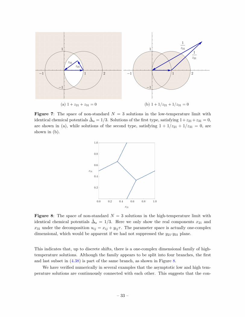
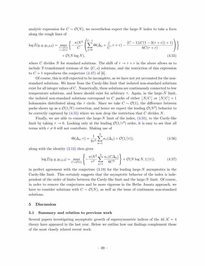