Asymmetric benchmarking in compensation: Executives

are rewarded for good luck but not penalized for bad∗

Gerald T. Garvey† Todd T. Milbourn‡

(Received 13 May 2003; accepted 14 January 2004)

∗JEL classification: D8; G3; J3 Keywords: CEO compensation; benchmarking; pay for luck Thanks to SendhilMullainathan (American Finance Association discussant), Harold Mulherin, Bill Schwert (editor), Richard Smith,Yisong Tian, Steven Todd, conference participants at the 2004 AFA meetings, seminar participants at ClaremontMcKenna College, Indiana University, Southern Methodist University, University of Arizona and York University,and especially an anonymous referee for very useful comments. Remaining errors are our own.

†Barclays Global Investors, San Francisco, CA 94105, USA‡John M. Olin School of Business, Washington University, St. Louis, MO 63130, USA

1

Abstract

Principal-agent theory suggests that a manager should be paid relative to a benchmark that

removes the effect of market or sector performance on the firm’s own performance. Recently, it

has been argued that such indexation is not observed in the data because executives can set pay

in their own interests; that is, they can enjoy “pay for luck” as well as “pay for performance.”

We first show that this argument is incomplete. The positive expected return on stock markets

reflects compensation for bearing systematic risk. If executives’ pay is tied to market movements,

they can only expect to receive the market-determined return for risk-bearing. This argument,

however, assumes that executive pay is tied to bad luck as well as to good luck. If executives can

truly influence the setting of their pay, they will seek to have their performance benchmarked only

when it is in their interest, namely, when the benchmark has fallen. Using industry benchmarks,

we find significantly less pay for luck when luck is down (in which case, pay for luck would reduce

compensation) than when it is up. These empirical results are robust to a variety of alternative

hypotheses and robustness checks, and they suggest that the average executive loses 25-45% less

pay from bad luck than is gained from good luck.

2

1. Introduction

Both the level and the stock-price sensitivity of executive compensation have increased dramat-

ically since the 1980s (Hall and Liebman, 1998). Academics (Bertrand and Mullainathan, 2001;

Bebchuk and Fried, 2003) and practitioners (Crystal, 1991; Rappaport, 1999) are concerned that

the boom in pay was at least in part a windfall. That is, executives were enriched for merely track-

ing a bull market. Consistent with this view, Bertrand and Mullainathan (2001) show that pay

is as sensitive to exogenous forces (henceforth, luck) as it is to firm-specific performance and that

the linkage is stronger when shareholders are diffuse and arguably more passive. (A similar finding

appears in the empirical literature on relative performance evaluation. See Antle and Smith, 1986

and Aggarwal and Samwick, 1999a, 1999b.)

Our starting point is the observation that an executive whose pay is tied to market movements

has relieved her shareholders of some of the firm’s systematic risk. By definition, the systematic

component of returns provides the fair-market rate of compensation for such services. The argu-

ment applies a fortiori to exogenous but unsystematic shocks such as those that affect only a single

industry. Tying compensation to such shocks reduces an executive’s expected utility because the

market provides no compensation for bearing such risks. Thus, the Bertrand and Mullainathan

(2001) result that the sensitivity of pay to exogenous luck is stronger when a large outside share-

holder is absent does not necessarily support their conclusion that such executives are able to set

pay in their own interests.

The above argument is based on the estimated sensitivity of compensation to various perfor-

mance measures. A typical regression coefficient implies that executives’ compensation changes by

$X for every $1,000 change in the market value of the firm’s equity, regardless of whether that

change is the result of firm-specific performance or exogenous luck. Our argument that pay for

luck only provides the executive with the market return in exchange for bearing systematic risk is

only valid if compensation retains its sensitivity to performance when luck turns out to be bad.

In this paper, we find evidence that executives are in fact insulated from bad luck, while they are

rewarded for good luck.1

1Betrand and Mullainathan (2001) note the appearance of such asymmetry but do not pursue the issue system-

3

The most straightforward interpretation of the data is as follows. At the beginning of any

compensation period, luck-based pay will be at best a zero-net present value (NPV) investment from

an executive’s point of view. It is equivalent to a zero-dollar investment position that yields the right

to participate in subsequent gains or losses in a set of market-priced assets. The expected return

on this position simply compensates the holder for the systematic risk involved. But compensation

is not completely determined in this ex ante fashion. Instead, it is decided at the end of each fiscal

year by the compensation committee of the board of directors (see, e.g., Crystal, 1991), at which

point it is known whether exogenous forces (luck) have turned out favorably or unfavorably for the

firm. At this stage, the executive’s self-interest is straightforward: Emphasize benchmarking and

remove exogenous influences from compensation only if the benchmark is down. This effectively

transforms the executive’s investment in the luck component of performance from a zero-NPV

appreciation right into a valuable option. The presence of this valuable option is exactly what we

find in the data.

Two additional tests further our understanding of the process whereby asymmetric benchmark-

ing takes place. First, the effect is stronger when corporate governance is weaker, according to

the measure introduced by Gompers, Ishii, and Metrick (2003). We argue that this makes sense

because executives strictly prefer asymmetric benchmarking to simple pay for luck. Second, part of

the phenomenon is attributable to stock option granting practices. O’Byrne (1995) and Hall (1999)

distinguish two alternative approaches to option grants: fixed-number and fixed-value. Fixed-

number granting policies give an executive the same number of options every year. Thus, if the

stock price goes up, the executive receives a more valuable grant as well as a capital gain on her

outstanding options. As Bertrand and Mullainathan (2001) point out, such a granting policy auto-

matically strengthens pay for luck. But executives prefer weaker pay for luck when luck turns out

to be bad. Fixed-value option granting policies increase the number of options granted when the

stock price has fallen in an attempt to maintain the total value of the grant. The usual justification

is to reduce the prospect of unwanted turnover (something that O’Byrne, 1995 terms “retention

atically. Our measures of luck include industry stock returns at the two-digit standard industrial classification codelevel. Thus, luck can be more broadly interpreted as the set of exogenous factors affecting a firm’s return, whichnaturally includes the effects of the market portfolio on average industry returns.

4

risk”). We find evidence that option-granting policies are closer to fixed-value when luck is bad

than when it is good. Put another way, compensation seems more concerned about retention risk

when luck is bad than with overpayment risk when luck is good.

Our empirical finding that top managers enjoy stronger pay for luck when luck is good is robust

to a host of potential benchmark portfolios and specifications. Nonetheless, there are several viable

alternative explanations. First, what we have in essence shown is a departure from linearity in the

pay for luck relationship. The slope is less steep below zero than it is above zero. But optimal

compensation need not be linear in stock market performance. If it is not, and firms do not bother

benchmarking, the asymmetry that we document could simply mirror the shape of the optimal

relationship between pay and firm-specific performance (henceforth, we refer to this portion of firm

returns as “skill”).2 We find, however, that the asymmetries in pay for luck and skill are statistically

different from one another.

Oyer (2004) and Himmelberg and Hubbard (2000) argue that benchmarking is not observed

in compensation because the value of executives’ outside opportunities are also market sensitive.

This can explain the absence of benchmarking when the market is up; the executive’s market

opportunities are also up and she would quit if the firm tried to benchmark her. But we find that

executives are benchmarked when the market is down. The Oyer (2004) story can explain our

results only if there is also an asymmetry in the sensitivity of executives’ outside opportunities

to the market. A related version of the labor market argument is that executives possess outside

opportunities that are not related to the overall market at all. Examples include working in the

non-profit sector, writing a book, or pursuing some other form of outside personal interest. This

would imply that in a down market, the firm still needs to provide the executive with a minimum

level of compensation to keep her from taking such opportunities. An observationally equivalent

idea is that the Chief Executive Officer (CEO) is essentially infinitely risk-averse with respect to

reductions in pay. This minimum-pay hypothesis, however, has the same empirical implication

as the mirror-image hypothesis outlined above. If the manager has a fixed minimum amount of

2Jin (2002) shows that the lack of indexation for the average executive is consistent with efficient contracting.Moreover, Garvey and Milbourn (2003) show that indexation occurs in circumstances in which it would appearefficient, providing managers with insurance when they can least provide for it themselves.

5

compensation she must receive, her pay will show the same asymmetric response to luck and to

skill. We are able to reject this hypothesis in the data.

Another alternative explanation is that executives do indeed suffer losses from bad luck, but such

losses take the form of dismissal or turnover. We find, however, that turnover has no statistically

significant association with luck and thus no evidence that dismissal is the punishment for bad

luck. Finally, the asymmetry between pay for good versus bad luck could reflect an asymmetry in

firms’ underlying exposure to luck. Firms with appropriate flexibility can reap the gains to good

markets while leaving some of the losses from bad luck to be borne by their less flexible rivals. We

show that this can explain our results only if flexible firms have stronger pay for performance. We

find no evidence to support this condition in a simple test exploiting the fact that flexible firms

will also tend to show systematically higher levels of skill.

The remainder of this paper is organized as follows. Section 2 presents a simple model in

which pay for luck need not be desired by executives and then delineates our empirically testable

hypotheses. Section 3 contains our primary empirical results and several robustness checks, while

in Section 4 we provide tests of alternative hypotheses. Section 5 contains additional tests of the

source of the skimming results we uncover. Concluding remarks are in Section 6.

2. A simple model of pay for luck

To fix ideas, we first provide a simple model of executive pay in order to tease out our empirical

hypotheses.

2.1. Basic results

We consider a one-period model of an all-equity firm employing a single manager. The executive

is paid according to firm value, where initial value is denoted V and its end-of-period value is denoted

V1 = V (1 + βrm + δL+ ε). (1)

For simplicity, we normalize the risk-free rate of interest to zero and set the scale factor V = 1.

Following standard notation, rm represents market returns and β is the firm’s sensitivity to this

market factor. The second shock L is luck and could represent returns to the firm’s industry, oil

prices, exchange rates, or any other objective index that affects the value of the specific firm. The

6

term δ represents the sensitivity of firm value to luck, and ε is firm-specific risk (or skill), unrelated

either to the market or to what we term luck. We assume that market risk is priced but that both

luck and skill are diversifiable, so that E(rm) > 0 and E(L) = E(ε) = 0. All shocks are assumed to

be independently and normally distributed. The results in this section generalize straightforwardly

to a setting with multiple systematic factors and multiple luck factors.

Because the terms rm and L are both verifiable, the executive’s pay can be separately condi-

tioned on both factors. To economize on notation, we assume that the firm chooses to link some of

the manager’s pay to firm value, but do not model the underlying incentive problem that motivates

such a compensation arrangement. The manager’s pay is assumed to take the form

W = w + a(1 + ε) + bmrm + bLL, (2)

where w represents fixed pay, a is the sensitivity of pay to idiosyncratic firm value (skill), bm is

the extent to which the manager is paid for market movements and bL is the sensitivity of pay to

luck. In a standard principal-agent setting, the term a would represent the marginal reward the

manager receives for effort given that her efforts cannot be disentangled from other firm-specific

determinants of value.

If the firm makes no attempt to distinguish exogenous forces (market and luck) from firm-specific

outcomes, we will observe bm = aβ and bL = aδ. That is, the manager is paid as much for market

movements and luck as she is for firm-specific performance. Bertrand and Mullainathan (2001)

find evidence that this is the case and argue that this is evidence that at least some executives

have captured the pay process, thereby enabling them to enrich themselves at the expense of

shareholders. To analyze this claim, however, it is not sufficient to point to cases in which either

βrm is large and positive (i.e., the market has gone up and the firm has a positive beta) or that W

increased because of good luck (δL). If an executive has in fact captured the pay process, she will

certainly exploit this fact to increase her expected utility. To address this question, we assume that

the manager has negative exponential utility with a coefficient of risk-aversion given by k. This

allows us to write the certainty-equivalent of her utility in terms of the mean and variance of her

7

compensation, given by

U = w+ a+ bmβE(rm)− k

2

£a2σ2e + b2mβ

2σ2m + b2Lδ2σ2L

¤. (3)

Bertrand and Mullainathan (2001) show that, on average, managers are paid for luck. That is,

bm and bL are both positive. However, whether such an arrangement increases the CEO’s expected

utility depends on the signs of the following3

∂U

∂bm= βE(rm)− kbmβ

2σ2m and (4)

∂U

∂bL= −kbLδ2σ2L . (5)

The first term ( ∂U∂bm) could be positive or negative. Linking the executive’s pay to market-wide luck

increases her expected utility only if bm < E(rm)kβσ2m

. This result has a natural interpretation. Because

the expected market risk premium is positive, the executive desires some exposure to its shocks.

She gains from such exposure so long as it is not excessive, given her risk aversion. The results

on pay for luck are even simpler. The term ∂U∂bL

is unambiguously negative. The executive strictly

prefers to be insulated from luck because it is risky and the market provides no compensation

for bearing such risks. If an executive has captured the pay process, we would ultimately expect

bL = 0.

2.2. Results when executives have access to capital markets

The results above are similar to those in the standard principal-agent literature in which pay

is set to maximize shareholder wealth, subject to participation and incentive constraints, rather

than to enrich the executives. The interpretation is that it is inefficient to have the manager bear

risks that the shareholders can bear at lower costs if there are no incentive effects. Here, the

interpretation is that even if the manager can choose her own pay, she will not choose to expose

herself to risk when the compensation is insufficient.

Our results imply that the Bertrand and Mullainathan findings are not necessarily consistent

with their conclusion that at least some managers have captured the pay process. We say ‘not3We take partial derivatives with respect to bm and bL and do not consider the possibility that the fixed component

w changes to compensate for any utility losses or gains. We ignore this because to implement it empirically wouldrequire direct estimates of executives’cash compensation, which are observable, but also requires direct estimates oftheir outside opportunity wages, which are unobservable.

8

necessarily’ because our model implies that bL = 0, but bm = E(rm)kβσ2m

. That is, the manager not

only will choose pay to insulate herself fully from luck, but also to give herself an optimal positive

exposure to the market. Betrand and Mullainathan cannot reject the hypothesis that bm = a/β.

That is, pay is equally sensitive to market and to idiosyncratic shocks to value. Absent information

about the manager’s risk-aversion k, we cannot reject the hypothesis that managers are receiving

their most preferred exposure to market shocks through their pay arrangements.

Jin (2002) and Garvey and Milbourn (2003) point out that the above analysis ignores the fact

that executives can and do choose securities such as mutual funds for their own private portfolios.

However, thus far the analysis assumes that they can invest in various markets only implicitly

through their compensation. Suppose to the contrary that the manager can also choose to invest

cm dollars of her risk-free wealth w in the market and cL dollars in a security that tracks the luck

factor (an industry index or oil futures, for example). Because the risk-free rate is zero, we can

now write her expected utility as

U = w + a+ (bmβ + cm)E(rm)− k

2

£a2σ2e + (bmβ + cm)

2σ2m + (bLδ + cL)2σ2L

¤. (6)

Her private investment choices will satisfy the following first-order conditions

∂U

∂cm= E(rm)− k(bmβ + cm)σ

2m = 0 and (7)

∂U

∂cL= −k(bLδ + cL)σ

2L = 0. (8)

In light of her optimal private holdings, the effect of pay for luck on her expected utility is given

by

∂U

∂bm= βE(rm)− βk(bmβ + cm)σ

2m = 0 and (9)

∂U

∂bL= −kδ(bLδ + cL)σ

2L = 0. (10)

As long as the executive can make her optimal private investment choices cm and cL, she is

indifferent to the sensitivity of her pay to either market shocks or luck. She can always create her

most desired exposure to the market or to luck, regardless of how her pay is determined. This

result also carries over if the executive believes she has private information about either the market

9

or luck. She can equally well take bets through her compensation or through her own private

investments.

Garvey and Milbourn (2003) recognize that at least some executives will not be able to freely

choose their own desired investment positions. Legal restraints, transaction costs, or limited per-

sonal wealth, for example, could prevent her from taking large short positions in either the market

or her industry. Our basic point still holds, however. Markets and industries go down as well as

up, and an executive gains no obvious benefit from being exposed to such risks through her pay.

Sometimes she will prosper from good luck, but other times she will suffer from bad luck.

2.3. Second thoughts: asymmetric benchmarking?

Bertrand and Mullainathan (2001) refer to the phenomenon of pay for luck as managerial

“skimming.” This terminology suggests that perhaps managers skim off only the gains stemming

from good luck. Bertrand and Mullainathan note the appearance of an asymmetry for oil price

shocks but do not present systematic tests. The fact that executive stock option exercise prices

are frequently revised downward after price declines but never, to our knowledge, upward to offset

price increases suggests a similar asymmetry (see, e.g., Chance, Kumar, and Todd, 2000). Similar

cases exist in the determination of bonuses. Under existing accounting standards, a portion of

the investment gains and losses on pension plan assets are recorded as income. During a market

upswing, pension gains help increase a firm’s net income and ultimately the CEO’s bonus payout.

However, as markets fall, pension losses reduce net income and, in theory, the CEO’s bonus.

In response to the economic downturn, many firms, including GE, Delta Air Lines, AK Steel,

and Verizon, apparently amended the compensation formula (Wall Street Journal, 2003 ). One

particularly glaring example was identified at AK Steel, where “[i]n January 2003, two weeks

before announcing the full-year loss for 2002, the company amended the terms of its annual bonus

plan, so that bonuses would be pegged to net income ‘excluding special, unusual and extraordinary

items.’ The company similarly amended its long-term incentive plan.”

Affording a board of directors some discretion over bonus payouts need not result in such

apparently perverse results. Discretion can be optimal in situations in which monitors (e.g., the

10

board of directors) have access to valuable, yet subjective, information surrounding a manager’s

performance. Murphy and Oyer (2003) document several cases in which bonuses owed to top

executives based on objective criteria were disallowed by the board based on “poor individual

performance [or] underperformance relative to similar firms.” Thus, there exist individual cases

where benchmarks are both used appropriately and where they appear instead to enrich executives.

Our tests help identify which of the two is more likely to be observed in the broader marketplace.

The following simple model details and clarifies the empirical implications of our argument.

The starting point is the recognition that actual compensation, including the use of benchmarks,

is not completely determined by a contract. Instead, it is chosen by the compensation committee

of the board each year, looking back at past performance. This shifts the focus from ex ante

contracting and welfare to ex post outcomes. Here, ex post means after the realization of luck has

been revealed. To simplify, focus on one dimension of luck L and associated pay for luck b. Based

on the evidence that little benchmarking exists on average, suppose that the default arrangement

is one in which pay is as sensitive to luck as it is to skill (b = a). However, the executive can induce

the board to evaluate and pay her relative to the benchmark L by exerting influence at a cost of I

to the executive. Thus, she can shift from a pay for luck regime in which b = a to a benchmarking

regime in which b = 0. It is rational for the executive to incur the cost I only if it is exceeded by

the loss she avoids by being benchmarked, an amount equal to aL. Thus, below the critical luck

level of − Ia , we will observe benchmarking and for L > − I

a we will observe pay for luck. This is

illustrated in Panel A of Fig. 1.

The above argument not only helps lay out our empirical implications, but it also indicates the

barriers to successful testing. First, we cannot observe the influence cost I, although we follow the

logic of Bertrand and Mullainathan (2001) in arguing that I is lower when governance is weaker.

Second, there is no reason to presume that the costs of influence are all fixed. If there are increasing

marginal influence costs, we will see a smooth movement from b = 0 to b = a as L increases. This

is illustrated in Panel B of Fig. 1 for the case in which influence activities reduce b one for one

at the strictly increasing cost of I2/2 . Third, if the default is full benchmarking and not pay for

11

luck, the critical luck value in Panels A and B would be the positive number Ia , at which point

the executive exerts effort to shift her pay from benchmarking toward pay for luck. In all cases,

however, we have the result that there should be less pay for luck when L < 0 (benchmark is down)

than when L > 0 (benchmark is up).

Insert Fig. 1 near here

3. Empirical analysis

In this section, we describe our data, lay out our empirical methodology, and ultimately provide

our main results.

3.1. Data and descriptive statistics

Our data are drawn from two sources. Firm returns and estimates of their volatility come

from the Center for Research in Security Prices (CRSP), and the compensation data are drawn

from Standard and Poor’s ExecuComp. Our sample period covers the years 1992 through 2001,

and Panel A of Table 1 summarizes the basic compensation and firm-specific variables for the full

sample. These summary statistics cover each firm’s executive identified by ExecuComp as the

CEO given by the CEOANN field. We drop firms with fiscal years ending in any month other

than December because we need to use peer group performance as a benchmark. Finally, because

we need to analyze year-to-year changes in compensation, we drop firm-years in which the CEO

was changed and in which the CEO served for less than two full years. We address the resulting

selection issues in two ways. First, Panel A of Table 1 presents summary statistics from the full

ExecuComp sample, whereas Panel B contains the same summary statistics for the subsample we

employ in our analyses. Our subsample is not qualitatively different from the full sample. Second,

we explicitly analyze the effects of what we estimate as luck and skill on CEO turnover in Section

4.

Insert Table 1 near here

Focusing on our usable subsample in Panel B, salary and bonus represent the CEO’s yearly

salary and bonus values, respectively, and average to approximately $634,000 and $703,000. Option

12

grants represents the Black and Scholes value of the options granted to the CEO in the year and

average just under $2 million. CEO age is the CEO’s age in the data year, and CEO tenure is

calculated as the difference in years between the fiscal year-end of the current year and the date

at which the executive became CEO, as given by the became_CEO field. Stock return is the

one-year percentage return for the firm over the calendar year (which also is the firm’s fiscal year

because we focus only on December fiscal year-ends), and market cap of equity is the firm’s market

capitalization at the end of the year. The standard deviation of stock returns are computed

using the monthly returns of the five years preceding the data year. Not surprisingly, requiring

multiple firm-years with the same CEO tends to favor more established firms with more fixed

pay, slightly lower volatility and returns, and slightly higher market values. All differences are

slight, however. The more important feature of both the full sample and the subsample is the

enormous right skewness in the data. For instance, the maximum value of option grants is over $60

million, and the median value is approximately one-fourth of the mean. To reduce the effects of

such outliers, our variables of empirical interest are all winsorized at the 1% level and we estimate

robust standard errors.4 We ignore changes in the value of the CEO’s existing shares and options

because by definition they move only with the stock price and cannot have distinct sensitivities to

luck versus skill.

While our theoretical model distinguishes between two exogenous shocks to firm value (market

and luck), actual firms are subject to a large number of such shocks. In Table 2, we provide summary

statistics for the two benchmarks we use. These include both the equal-weighted and value-weighted

industry returns, in which a firm’s industry is given by the remaining ExecuComp firms in the same

two-digit standard industrial classification (SIC) code. Critical to our ability to test the hypothesis

that managers opportunistically benchmark their pay is the fact that the benchmark can take both

positive and negative values. To that end, Table 2 summarizes the percentage of the observations

for each benchmark that are positive, as given in the column denoted “percent positive”. Not

surprisingly for our sample period, a large proportion of our sample contains positive benchmark

4Our regression results are also robust to the use of median and robust regressions, which also minimize the effectof outliers on coefficient estimates. We report the estimates of median regressions in Tables 5 and 6.

13

returns.

Insert Table 2 near here

It is important to note that our empirical results are robust to a wide variety of luck measures,

including broader market-based measures such as the value-weighted and equal-weighted market

return, size decile-based returns, and even more focused measures of luck such as oil price move-

ments. All of these are imperfect measures of luck, and empirically we cannot be certain that we

have adequately distinguished between the portion of a firm’s return given by luck and that which

is affected by the executive’s actions and decisions (i.e., her skill). We will inevitably misclassify

some luck as skill, and vice versa, and such measurement error will tend to push the estimated pay

coefficients on luck and skill closer together. Because our tests are based on estimating different

coefficients on luck and skill, simple measurement error biases us against finding this result. We

also deal in some detail with a related alternative explanation in which firms’ exposures to luck are

not linear as we assume in our model specification (see Section 4.1).

We provide simple correlations of some key variables in Table 3. Not surprisingly, both option

and total compensation have a strong and positive association with firm size as given by its market

capitalization and also with percentage stock returns and risk. Remaining correlations are typical

of other compensation studies.

Insert Table 3 near here

3.2. Pay for luck confirmed

We begin our analysis by confirming the result that the average executive receives compensation

for exogenous as well as firm-specific performance. We follow the Bertrand and Mullainathan (2001)

approach of breaking the test into two stages. First, firm performance (given here by the firm’s

raw stock return) is regressed on exogenous components, given by the equal-weighted and value-

weighted industry returns, with the resulting predicted value representing what we coin luck and the

residual representing skill (i.e., the firm-specific component of firm performance).5 This provides a

5We do not include market returns because our estimates all include time dummies. Because market-wide returnsvary only by year, they add no information in this setting.

14

natural and parsimonious way to deal with the large set of potential indices. In terms of the model,

we estimate the regression

V1 − 1 = βrm + δL+ γX + ε, (11)

where ε is the residual from the regression and X represents the indices plus year dummies.6 The

model normalizes beginning of period value to one. In our regressions, we scale both firm returns

and the returns on the indices by each firm’s market capitalization at the beginning of the year.

We then compute the luck component of firm returns as

λ = bβrm + bδL+ bγX, (12)

where bβ, bδ, and bγ are the estimated coefficients from Eq. (11). Summary statistics on our empiricalestimates of luck and skill are contained in Panel B of Table 4.

Insert Table 4 near here

To test the effect of luck versus skill on compensation, we follow the approach of Aggarwal and

Samwick (1999a) on the pay for performance relationship.7 First, we use changes in compensation as

the dependent variable. Second, we use dollar performance measures for both luck and skill, which

involves multiplying predicted and residual stock returns by market capitalization at the beginning

of the year. Third, and most important, we follow Aggarwal and Samwick and depart from Bertrand

and Mullainathan (2001) by not fixing the sensitivity of pay to either luck or skill to be the same for

all firms. Instead, we include interactions between luck and skill and the cumulative distribution

function (cdf) of their own respective volatilities. Aggarwal and Samwick show that ignoring this

6Bertrand and Mullainathan (2001) also include firm fixed effects in their performance regressions. This effectivelysays that each firm’s average performance over the sample period, even after controlling for market and industryeffects, was due to exogenous luck. While our results are qualitatively unaffected by adopting their specification, weomit firm dummies from the performance regression.

7Bertrand and Mullainathan (2001), along with many other compensation studies, also use log-log specifications.As stressed by Baker and Hall (2004), theory does not dictate which specification is preferable and our resultsare similar with the log specification. We report results with the linear specification for two reasons. Empirically,we estimated Box-Cox specifications in which compensation is transformed to (Compθ − 1)/θ and the maximum-likelihood estimate of θ was 1.12. This estimate of θ was insignificantly different from one (implying that theunderlying relationship is linear), but was significantly different from zero (implying that the underlying relationshipis not log). If we applied the transformation to both compensation and performance (luck and skill), the θ estimatewas 0.92, again indistinguishable from one, but statistically different from zero. Theoretically, our hypotheses aboutasymmetric benchmarking essentially point to a local convexity in the compensation function, which shows up mostnaturally if we do not perform a concave transformation on the data.

15

heterogeneity systematically understates the strength of the pay-performance relationship. (We use

dollar variance because we are regressing dollar compensation on dollar stock returns.) Thus, our

variance measure captures both size and percentage risk effects. This is not a problem for Bertrand

and Mullainathan because their question is whether pay is equally sensitive to luck and skill and

also because we find their result carries over to the case in which the sensitivity is allowed to differ

according to risk. But we need to estimate the attenuation of the pay for luck relationship when

luck is down, and thereby require an accurate estimate of this relationship as a first step. In terms

of our empirical model, we estimate

W = w + aV ε+ bV λ+ cV ε× cdf(V ar(V ε)) + dV λ× cdf(V ar(V λ)) + gY , (13)

where Y contains controls for firm fixed effects, year effects, total risk, and the CEO’s tenure.

In the first regressions of Panel A of Table 4, we defineW as the change in total direct compensa-

tion, which reflects salary, bonus, long-term incentive payments, all other compensation, the market

value of restricted stock granted, and the Black, Scholes and Merton value of options granted. In

the second and third regressions, we separately treat the two main sources of incentive pay: bonuses

and option grants.

We immediately confirm the Bertrand and Mullainathan (2001) finding that executive pay is

positively and significantly related to both luck and firm-specific performance. That is, we estimate

that both bb > 0 and ba > 0. Consequently, the conclusion to be drawn from Panel A of Table 4

is the standard one: indexation (or benchmarking) is not an important feature of the average

executive’s compensation. The point estimates of the coefficients imply that for a CEO of a firm

with median risk, an additional $1,000 in firm value from skill (which is unrelated to industry or

market conditions) will increase total compensation by 96 cents [1.823−(12×1.725)], bonus payoutsby just under 31 cents, and new option grants by 42 cents. While this represents substantial pay for

performance (and significantly understates actual incentives because we omit the ongoing incentives

resulting from previously granted shares and options), the same executive will gain 74 cents in total

compensation, 18 cents in bonus, and 35 cents in larger option grants for performance that is entirely

the result of market or industry factors (i.e., from luck). In no case are the sensitivities to luck and

16

skill statistically different from one another.

These findings are similar to those that led Bertrand and Mullainathan (2001) to conclude that

at least some executives skim the gains to luck. However, as argued in our model, such a finding is

also consistent with executives bearing exogenous risks that neither increase their expected utility

nor decrease shareholder wealth. Below, we present our main findings of differential indexation in

compensation as a function of realized luck.

3.3. Evidence of asymmetric indexation

As shown in Section 2.3, the most durable and robust prediction of our idea is that there will

be less benchmarking when the benchmark is down than when it is up. The actual break point

need not be at zero, and we take this point up in Subsection 3.4.

As indicated in the Introduction, optimal contracting provides an alternative explanation for

the asymmetry. The optimal incentive contract based on skill could have a nonlinearity near zero.

Such a contract could be optimal to encourage managerial risk-taking, or because such outcomes

are revealing of the agent’s effort (see Hart and Holmstrom, 1987). The firm could also decide that

it is optimal not to benchmark the executive (see Jin, 2002, and Garvey and Milbourn, 2003). If

so, the apparent nonlinearity in pay for luck is simply the mirror image of an optimal incentive

contract based on skill. Our first test of these hypotheses involves allowing the sensitivity of pay to

luck and skill to differ depending on whether luck or skill, respectively, is up or down. Specifically,

we add the following interaction terms to our specification in Eq. (13):

aDV ε×D1(ε < 0) + bDV λ×D2(λ < 0), (14)

where D1(ε < 0) is an indicator variable taking on the value one if skill is negative, and zero

otherwise, and D2(λ < 0) is the analogous indicator variable for luck. The skimming hypothesis

predicts that bD < 0. The optimal contracting hypothesis can also explain an empirical finding

that bD < 0 but would also imply that aD = bD. We empirically examine these coefficients next.

In Table 5, we summarize the estimated coefficients from three specifications using changes in

total direct compensation, followed by estimates of models of changes in the two most important

discretionary components of compensation: bonus payouts and option grants. Not surprisingly,

17

salary and the other components of compensation show negligible sensitivity to either luck or skill.

The first column is our primary specification, allowing for both pay for luck and pay for skill to

be asymmetric around zero. The second column omits the skill interaction term to ensure that

the asymmetry in pay for luck remains even when we restrict pay for skill to be linear. The third

column estimates a median regression (minimizing the sum of absolute errors instead of squared

errors) to ensure that our results are not driven by outliers. The last two columns repeat our

primary specification restricting attention to bonuses and to option grants, respectively.

Insert Table 5 near here

As in the results of Panel A of Table 4, we estimate a positive and significant relationship

between changes in total executive pay and the realizations of luck and skill, with both effects

weakening as the firm becomes riskier. More importantly, we estimate a negative coefficient for

bD that is both statistically and economically significant whether or not we allow for asymmetry

in pay for skill and regardless of the estimation method. Moreover, we consistently reject the

hypothesis that the asymmetry in pay for bad luck and pay for bad skill are equal (i.e., aD = bD).

The results also continue to hold if we remove those cases in which compensation (total, bonus,

or option grants) is at its lower bound of zero. Thus, our finding that executives are insulated

from bad luck is not driven by the fact that they cannot receive negative compensation when luck

is particularly bad. However, they can still receive their punishment for bad luck in the form of

dismissal, and we take up this alternative explanation later.

The findings summarized in Panel A of Table 4 suggest that, on average, the executive’s pay is

affected by luck. However, the results of Table 5 show that the executive is rewarded more for good

luck than she is punished for bad luck. Our point estimates imply that the executive at a firm with

median risk receives approximately 79 cents [1.413 − (12 × 1.243)] in additional compensation forevery additional $1,000 increase in shareholder wealth because of luck. On the other hand, she loses

only 60 cents (given by the sum of the median pay for luck sensitivity of 79 cents and the estimated

coefficient on bD = −19.2 cents) for every $1,000 loss in shareholder wealth due to bad luck, areduction of almost 25%. The proportional reduction in exposure to bad luck is greater still when

18

we use median regressions, because estimated pay for luck falls more than the estimated asymmetry

at zero luck. Equally important, no such favorable asymmetry (from the executive’s perspective)

is evident in the skill component. In some specifications, the manger is punished somewhat more

for bad skill than she is rewarded for good skill.8

The primary contribution of our work is that we empirically test the most natural implication

of the skimming approach that provides a strictly different prediction than standard agency theory.

That is, if top managers can in fact influence the form of their compensation, they will seek

indexation (i.e., insurance) only when it is to their advantage to do so. Ex post, insurance is

valuable to the manager only when unfavorable outcomes are realized, and this is what our first

set of tests strongly suggest. The remainder of the paper supplements these results. We first

estimate piecewise linear regressions to push the theory’s predictions to their limit and then address

alternative explanations for the results. Finally, we attempt to uncover possible sources of the

skimming we have identified.

3.4. Testing the break point and functional form

The ex post model (and accompanying Fig. 1) sketched at the end of Section 2 suggests that

the relationship between b and L is neither globally concave nor convex. Instead, there should

be a significant increase in the estimated coefficient on luck (b) moving from large and negative

realizations of luck to values that are closer to zero, with little subsequent increase thereafter.

Unfortunately, the appropriate breakpoints are not clear a priori because of the unobservability

of both the managerial influence costs (I) and the underlying relationship between these influence

costs and the resulting sensitivity of pay to luck. Therefore, in Table 6, we estimate piecewise

linear models using various breakpoints for luck that bracket the value of zero. Using the summary

statistics on luck and skill from Panel B of Table 4 as a guide, we consider two sets of breakpoints

based on percentiles. In each of these cases, the critical value of zero lies strictly between the

breakpoints.

8This is not to say that the average executive has incentives to reduce risk. We have ingored convexity andpay-performance incentives stemming from options already granted because these must have the same sensitivity toluck and skill. This is also why our estimated sensitivities are less than those in Aggarwal and Samwick (1999a) anbdMilbourn (2003).

19

Insert Table 6 near here

We amend Eq. (13) by segmenting the contribution of exogenous factors (luck) to the firm’s

dollar returns (bV λ) into

bLowV λ{Low} + bMedV λ{Med} + bHighV λ{High}, (15)

where

λ{Low} =

⎧⎪⎨⎪⎩ λ if λ < 10th percentile of λ

0 otherwise,(16)

λ{High} =

⎧⎪⎨⎪⎩ λ if λ > 90th percentile of λ

0 otherwise, and(17)

λ{Med} =

⎧⎪⎨⎪⎩ λ if λ ∈ [10th, 90th percentiles of λ]0 otherwise.

(18)

We similarly segment the contribution of firm-specific factors (skill) in that we also include

aLowV ε{Low} + aMedV ε{Med} + aHighV ε{High} (19)

in some specifications. Given the lack of theoretical basis for the exact breakpoint, we also report

results for the less extreme case in which low luck is defined as luck below the 20th percentile and

high luck is above the 80th percentile.

Our chief hypothesis is whether the pay for luck coefficient in the lowest range of luck is less

than the others because it contains values in which the executive would strictly prefer no pay for

luck. The secondary hypothesis is that the medium coefficient is less than the high coefficient

because the executive is willing to expend more resources to tie her pay to luck as luck increases.

To test these hypotheses, we rely on median regressions as in Aggarwal and Samwick (1999a) that

minimize the sum of absolute instead of squared errors. Results are qualitatively similar if we

use ordinary least squares (OLS), but the coefficients on high and low are strongly affected by

extreme values, while the medium coefficient is unaffected. Such issues are unavoidable because by

construction the λ(Low) range contains the extreme negative values of luck and the λ(High) range

20

contains the extreme positive values. Aggressively trimming the outliers is unappealing because of

the potential loss of valuable and scarce information from the extreme values of luck. We therefore

adapt our estimation technique instead of the data to suit the task at hand.

In the first two columns of Table 6, we designate the extreme deciles as high and low luck (and,

respectively, high and low skill, in the case of the second column). In the third column we expand

the definition of high and low luck to include the next highest and lowest deciles. In all cases,

the coefficient on low luck (bLow) is substantially lower than that on bMed and bHigh, although all

are positive and significantly different from zero. F -tests reject the hypotheses that the coefficient

on low luck is equal to those on either medium or high luck at the 1% level. This buttresses our

findings from Table 5 (where our results are tied to the breakpoint of zero) that there is less pay

for luck when luck turns out to be bad (i.e., when the realized value of luck lies in the lower range).

Equally important, we find no such pattern with the skill component of performance and thus no

support for the mirror-image explanation of our results.

While we find strong evidence that executives are insulated from bad luck, we do not find

evidence that they reap extraordinarily high rewards for good luck. In no case can we reject the

hypothesis that bMed and bHigh are equal to one another. This pattern is entirely consistent with the

model sketched in Fig. 1, and indicates the empirical relevance of the constraints we have assumed

on managerial skimming. First, executives do not seem able to fully avoid the consequences of bad

luck. The coefficient on low luck is about 50% smaller than that on higher levels of luck but is still

positive.9 Second, executives are not able to exploit the gains of good luck to an increasing extent

as luck improves. Instead, pay for luck is clearly bounded on the upside by the strength of the pay

for skill relationship. That is, executives can reap rewards for good luck only to the extent that

their pay is also tied to skill.

4. Alternative explanations

The results thus far strongly support the conclusion that executives can reap the rewards of

good luck without sharing proportionately in the losses from bad luck. In this section, we examine

9An alternative explanation for the finding that executives are not fully insulated from bad luck is measurementerror in the first-stage decomposition of performance into luck and skill. If the true relationship is that the executiveis fully insulated from bad luck, we could get our results simply by misclassifying some skill as luck and vice versa.

21

explanations other than executive skimming for this result. Section 5 then attempts to draw out

some of the mechanisms that underlie the ability of at least some executives to gain more from

good luck than they lose from bad luck.

4.1. Performance nonlinearities

A logical alternative explanation for our results is that pay is effectively linear in both luck and

skill, but firm performance is not. Specifically, a skillful manager could be able to adjust quickly to

exploit good luck or to avoid some of the consequences of bad luck or both. Of course, this cannot

be true for all firms in an industry or market; some must be in the opposite position of being

disproportionately exposed to bad luck.10 The simplest possible model of this argument would be

as follows. Consider an industry with two firms, one common shock L, and no firm-specific shocks.

The common shock L ∈ {−1, 0, 1}. The firms are identical in size, but the flexible firm’s CEOmanages to capture all of the positive shock and avoid all of the negative shock. Thus, the flexible

firm’s returns take on the values Vf ∈ {0, 0, 1} while that of the inflexible firm takes on the values

Vi ∈ {−1, 0, 0}. Panel A of Fig. 2 depicts the possible outcomes and the consequences of ignoringnonlinearity in performance in estimating each firm’s luck. When luck is good, the flexible firm has

a dollar return of one and the inflexible firm has a return of zero; our linear estimate will indicate

that both had luck worth 1/2 and ascribes the remaining performance to skill (1/2 for the flexible

firm, −1/2 for the inflexible firm). Similarly, when luck is bad, we will estimate luck = −1/2 forboth firms with the flexible firm again having skill = 1/2 (because it achieved a zero return when

luck was bad) and the inflexible firm again having skill = −1/2.

Insert Fig. 2 near here

To draw out the consequences for our estimated pay relationship, suppose that both firms link

pay to performance. Specifically, suppose the flexible firm pays its CEO a bonus f if its returns

are one and not zero, and the inflexible firm penalizes its CEO an amount −i if its returns arenegative one and not zero. Panel B of Fig. 2 depicts the resulting relationship that we will observe

10We thank the anonymous referee for suggesting the alternative explanation and for developing the idea to thispoint. However, we bear full responsibility for the developments that follow.

22

between pay and what we estimate as luck. Because we control for executive fixed effects, it is

reasonable to normalize pay to zero. When luck is good, the flexible CEO receives a bonus of f

and the inflexible CEO receives no bonus. When luck is zero, there are no bonuses or penalties.

When luck is bad, the inflexible firm penalizes its CEO −i but the flexible firm does not because

it has not suffered from the bad luck. We will therefore estimate a pay for luck sensitivity of f in

the good luck state (expected bonus is f/2 for luck = 1/2) and a pay for luck sensitivity of i in the

bad luck state (expected bonus is −i/2 for luck = −1/2).It is immediately apparent that performance nonlinearities can explain our observation of asym-

metric benchmarking if the flexible firm uses stronger incentives than the inflexible firm (f > i),

which is arguably a plausible hypothesis. Milbourn (2003) finds evidence that firms with better

past performance tend to tie their managers’ pay more closely to subsequent performance, but this

is not an appropriate test of the condition that f > i. Our observation is that flexible firm-CEO

pairs will tend to have positive residuals in our luck-skill regressions, and we can use this to clas-

sify firms to then test their contemporaneous pay-performance relationships.11 Milbourn’s (2003)

evidence implies that f > i only if there is strong persistence in abnormal stock performance over

multiple years, a condition that is not supported by the literature on momentum (e.g., Jegadeesh

and Titman, 1993), which finds that good performance tends to reverse after approximately six

months.

Before constructing a test of the condition f > i, it is important to note that our finding that

there is no systematic asymmetry in the pay-skill relationship is evidence against the nonlinear

performance explanation. The reason is that pay for what we measure as skill in this model is

exactly the same as pay for luck in Panel B of Fig. 2. The flexible firm has skill of 1/2 when luck

is good and when it is bad. When luck is good, its manager receives a bonus of f but no bonus

when luck is bad. Thus, the estimated return for good skill is also f . Similarly, the inflexible firm

has skill of −1/2 when luck is either good or bad but only bears the loss −i when luck is bad, sothe estimated loss for a unit of low skill is −i, just as for the case of bad luck.11 In presenting the model it was not necessary to carefully distinguish between firm and CEO because they formed

unique pairs. In the empirical tests, we focus on the skill of unique firm-CEO pairs.

23

Table 7 presents an additional test of the nonlinearity explanation, focusing on the condition

that flexible firms use stronger incentives than inflexible firms. The additional observation is that

flexible firms will tend to have systematically higher skill measures. In our model, the flexible firm

has skill of 1/2 when luck is good or bad, while the inflexible firm has skill of −1/2 in both cases. Foreach CEO-firm pair in our sample, we compute the median value of skill and ask if firms with skillful

CEOs have systematically higher pay for performance, when performance now makes no distinction

between luck and skill.12 The first column estimates an interaction term between performance and

the CEO-firm pair’s median skill level and finds no systematic evidence that higher skill CEOs

(and potentially more flexible employing firms) receive stronger pay-performance as required by

the asymmetric performance explanation for our results. The last two columns divide the sample

into CEOs with high and low median skill levels and show that, if anything, low-skill CEOs have

somewhat stronger pay-performance although the difference is not statistically significant. In no

case do we find empirical support for the asymmetric performance explanation’s key condition that

f > i. However, one reason we perhaps do not find it is that we are not directly measuring firm

flexibility, but instead proxy for it with median (or average) performance.

Insert Table 7 near here

4.2. External labor market forces

The skimming approach views compensation as an arena in which rent extraction takes place.

The specific ways in which managers extract rents are primarily through influence over the com-

pensation committee’s and regulators’ information and incentives. A related approach suggested by

Oyer (2004) and Himmelberg and Hubbard (2000) focuses on the managers’ threat of quitting not

only ex ante (as in the traditional principal-agent model), but also ex post, after performance has

been observed. This is a viable explanation for the existence of pay for luck if the manager’s out-

side opportunities fluctuate with market-wide outcomes. But they do not explain the asymmetry

between good and bad luck. An up-market could strengthen an executive’s outside opportunities

and hence her bargaining power, but a down-market should weaken such opportunities.12Similar results are obtained if we use average skill levels instead of median levels, but the classification of firms

is driven more by extreme values.

24

An alternative labor-market explanation is that the executive has some market-insensitive, out-

side opportunity to which she can revert, such as working at a nonprofit organization or writing

her memoirs. An observationally-equivalent explanation is that we have optimal ex ante incen-

tive contracts and executives are strongly averse to reductions in their pay below some minimum

(see, e.g., Scharfstein, 1988). This minimum pay hypothesis not only suggests why the executive

should be insulated from bad luck, but also implies that she should be insulated from firm-specific

downturns. We systematically rejected this hypothesis in the previous sections.

4.3. Job loss as punishment for bad luck

The labor market explanations assume that the managers’ outside opportunities provide her

with bargaining power through the threat of quitting and the associated turnover costs. There is

an alternative interpretation of turnover that could explain our results.13 Suppose that executives

are likely to be dismissed when the firm is experiencing bad luck. Because our sample contains only

those executives who remain on the job, and compensation cannot be negative, we systematically

underestimate the true punishment for bad luck.14

To test this explanation, we return to the full sample and code a dummy variable for years in

which the CEO position changes hands. We then ask if bad luck is associated with abnormally high

turnover in a probit estimate controlling for luck, skill, age, CEO tenure, firm size, and year effects.

The first column of Table 8 shows, consistent with the results in Barro and Barro (1990) for bank

executives and Brickley, Coles, and Linck (1999) for board members, that the turnover decision

appears to be benchmarked. That is, skill has a significant negative effect on the probability

of turnover, whereas luck has no discernible effect. Our second column asks whether bad luck

or bad skill have distinct effects on turnover, and suggests that if anything, there is asymmetric

benchmarking in dismissal as well as in compensation.

Insert Table 8 near here13Thanks again to an anonymous referee for suggesting this explanation.14 In our sample, approximately 15% of the bonus observations, 20% of the option grant observations, and 0.2%

of the total compensation observations are zero. All results continue to hold if we omit these observations, whichis to some degree expected at this point because any asymmetry induced by the zero minimum would also implyasymmetric pay for skill, counter to our results.

25

Dismissal is, a priori, a viable alternative explanation for our finding that pay increases in good

luck but does not symmetrically decrease with bad luck. Extreme punishment effectively requires

some kind of job change because pay cannot be negative. Given that the CEO is at the top of

the organization, the only unfavorable job change is to be dismissed. These facts undercut our

conclusion that executives are insulated from bad luck only if executives are disproportionately

likely to lose their jobs when luck is bad. We find no evidence to support this condition and

therefore maintain the conclusion that executives lose less from bad luck than they gain from good

luck.

5. Additional tests: how does skimming take place?

In this section, we provide two additional empirical tests to further explore how CEO pay

skimming actually takes place. To this end, we first examine whether skimming takes place more

often in situations marked by weaker corporate governance. Next, we explore whether boards alter

their option-granting policies as means of insulating CEOs against bad luck outcomes.

5.1. Governance and skimming

Bertrand and Mullainathan (2001) show that skimming (paying for luck) is weaker in firms for

which corporate governance is stronger. They proxy for the efficacy of corporate governance in

several ways: the presence of a large shareholder (holding a claim of 5% of the shares or more),

CEO tenure, board of directors size, and the fraction of board members who are insiders. The

presence of a large shareholder provides their strongest result, and they find that pay for luck is

reduced by as much as 33% in firms for which there is a large shareholder. They also find that the

presence of a large shareholder becomes more important for reducing CEO pay skimming as CEO

tenure increases.15

Absent readily available data on the presence of a large shareholder and both board composition

and size, we turn to the Corporate Governance Index constructed by Gompers, Ishii, and Metrick

(2003).16 This index is based on the prevalence of various corporate governance provisions at each

15Hermalin and Weisbach (1997) provide a theory that suggests CEOs with longer tenures will have greater influenceover the board of directors. However, we find that the severity of the asymmetric relationship of pay for luck isinsensitive to CEO tenure in our sample.16We thank Andrew Metrick for graciously providing us with these data.

26

firm and is inversely related to the strength of shareholder rights. That is, lower values of the

index correspond to greater shareholder (weaker management) rights, whereas higher values of the

index are associated with weaker shareholder (stronger management) rights. The key determinants

are takeover defenses, state laws, shareholder voting rights, and protection of directors and officers

through insurance and severance arrangements. In our sample, the index ranges from 2 to 17, with

a median and average value of 9 for the 5,377 firm-year observations for which we could match our

ExecuComp sample with that of Gompers, Ishii and Metrick. (The governance index spans the

range 2 through 18 in Gompers, Ishii, and Metrick, 2003.)

To form our testable hypotheses we adapt the logic of the Bertrand and Mullainathan (2001)

governance tests. CEOs should be better able to insulate themselves from bad luck outcomes when

they are employed by a firm with weaker shareholder rights (i.e., by firms with higher values of the

governance index). In the first and second columns of Table 9, we first replicate our analysis of

pay for luck in Table 4 for two subsamples of the data. In the first column, we examine the pay for

luck relationship in firms for which corporate governance can be characterized as strong (G ≤ 6).In the second column, we examine the same relationship in firms in which corporate governance

is weak (G ≥ 12).17 Similar to the results of Table 4, pay is positively and significantly related

to both luck and skill in firms with strong and weak corporate governance, respectively. This is

consistent with the original Betrand and Mullainathan (2001) findings. However, further consistent

with their findings, in the case of firms with stronger corporate governance, pay for luck is only

marginally significant and economically smaller than the associated pay for skill coefficient. This

is in contrast to the results for firms with weaker corporate governance where the estimated pay

for luck coefficient is strictly greater than the associated pay for skill coefficient.

We turn now to an examination of whether asymmetric indexation is in fact more prevalent in

firms with weaker corporate governance. In the third and fourth columns of Table 9, we replicate

the analysis of Table 5 on the strong and weak corporate governance subsamples by including the

17Gompers, Ishii, and Metrick (2003) rely on deciles of the index in their analysis of the effects of governanceon corporate performance. Here, we rely on quintiles so as to leave a sufficient number of firm-year observations(roughly 1,000) in each subsample. Qualitatively similar, yet statistically weaker, results are obtained using decilesas the breakpoints.

27

interaction of luck with an indicator of whether luck was negative. In the case of strong corporate

governance, we estimate a positive and significant coefficient (bD) on this interaction, consistent

with the notion that CEOs in better governed firms are not insulated from bad luck as in the average

firm. However, in the case of weaker corporate governance, CEOs are partially insulated from bad

luck with nearly 25% of the effects of bad luck removed from their ultimate pay. Thus, we conclude

on the basis of these results that while the average CEO’s pay is asymmetrically indexed (see Table

5), it appears to be marginally more prominent in situations in which the CEO could have greater

influence over her pay, such as is exemplified in a firm with weaker corporate governance.

This statement is further supported by the results contained in the fifth column of Table 9,

when we employ the full sample of firms. Here, we estimate the effects of asymmetric indexation

across three groups by including two additional interactions with our primary interaction of luck

with the indicator of whether luck was negative. We interact this primary interaction with an

indicator variable denoting whether the firm had strong corporate governance (G ≤ 6) and alsowith an indicator of weaker corporate governance (G ≥ 12). The asymmetric indexation for payat firms with intermediate quality of corporate governance is captured by the estimated coefficient

bD on the primary interaction. The natural prediction is that we should observe the least asym-

metric indexation in firms with stronger governance, moderate asymmetric indexation in firms of

intermediate governance strength, and the most severe asymmetric indexation in firms with the

weakest governance. Turning to our empirical findings, we see that the data are consistent with

the first two predictions, but not the third. That is, we observe no asymmetric benchmarking for

firms with G ≤ 6, significant asymmetric benchmarking for firms of intermediate governance, andinsignificant asymmetric benchmarking for firms with G ≥ 12. That said, we can strongly rejectthe hypotheses that the relevant bD coefficient for firms with good corporate governance is equal

to those at firms with either intermediate or weak corporate governance. We cannot, however,

reject the hypothesis that asymmetric benchmarking is the same at firms of intermediate and weak

corporate governance. Our inability to differentiate between these types of firms could simply re-

flect that once firms move away from the strong corporate governance set, an executive’s ability to

28

influence her pay strategically perhaps does not vary significantly. In any event, the results suggest

that the strength of shareholder rights does tend to restrain managerial pay-skimming practices.

5.2. Fixed value versus fixed number option granting policies

Hall (1999) shows that, on average, executives receive more valuable option grants when past

performance is better, but this is not universally the case. He distinguishes two basic alternative

option-granting policies. There are fixed-number granting policies, in which executives get more

valuable grants as firm value grows, and fixed-value granting policies, which attempt to hold the

yearly value of the option grant fixed even when price falls or rises. According to compensation

consultants (O’Byrne, 1995), the apparent goal in this latter policy is to maintain a constant ratio

of stock-based pay to fixed pay. Our asymmetric benchmarking story implies that firms would tend

to use a fixed-number granting policy when the stock price is driven up by exogenous forces, but

attempt to maintain the value of the option grant when luck is bad by increasing the number of

options granted.

The most direct test would be to regress the number of options granted on measures of luck

and skill, when the hypothesis is that the executive gets a distinct boost when luck is down. But

this would add little to our results in Table 5 where we show that the value of new option grants

is not much affected by bad luck. Since the value of a new (at-the-money) option is lower when

luck is bad, the total value of the grant can only be maintained by granting more options. This

is the essence of a fixed-value granting policy. Table 10 presents an alternative test based on the

recognition that if firms follow a strict fixed-value granting policy, a regression of the value of

option grants to a given CEO in year t on option grants to the same CEO in the previous year will

yield a coefficient of one. The first column regresses grants on lagged grants and all the empirical

controls used in Panel A of Table 4 (including risk, luck, skill, interactions of luck and skill with

risk, tenure, and year dummies). The exception is that we do not use firm fixed effects.18 Instead,

we control for two-digit SIC effects and also include other firm-specific determinants such as firm

size (measured by both the book value of total assets and the market value of the firm), the book-

18The reason is that, in this case, the lagged grant measure would capture only deviations from the firm’s ownsample mean grant value. If we employ firm fixed effects, we estimate a negative coefficient because, on average, anabove-average grant is followed by a below-average grant.

29

to-market ratio, and debt-to-total assets (see, e.g., Yermack, 1995). We then obtain the sensible

result that the coefficient on lagged option grants is positive and highly significant (firms do have

distinct and identifiable granting levels) and is also significantly different from one, implying that

some firms follow a fixed-number policy and, more generally, take into account other factors in

granting options.

The second column of Table 10 includes interactions between lagged option grants and both

bad luck and bad skill. The hypothesis is that if firms revert to fixed-value granting policies when

luck is bad, lagged option grants will be a stronger determinant of current option grants in such

times. Consistent with this, we estimate a positive coefficient on the interaction of bad luck and

lagged option grants. Bad luck drives the coefficient on lagged option grants about 10% closer to

the fixed-value level of one. Consistent with our previous estimates of the effects of bad luck versus

bad skill, we find that when firm-specific performance is bad, a tendency exists to depart further

from fixed-value granting policies and we can reject equality between the coefficients on bad luck

and bad skill interactions at the 1% level. The final column of Table 10 confirms that the evidence

that granting policies are closer to fixed-value when luck is bad does not rely on the inclusion of

the bad skill asymmetry term and its negative coefficient.

6. Concluding remarks

We find that executive pay is most sensitive to industry or market benchmarks when such

benchmarks are up. This is consistent with the view that important aspects of executive compen-

sation are not chosen as part of an ex ante efficient contracting arrangement, but rather as a way

to transfer wealth from shareholders to executives ex post. Normatively, the message is that the

choice of whether to remove luck from an executive’s compensation package is less important than

is consistency in this choice across years. That is, if the board chooses to use external benchmarks

to evaluate performance, these benchmarks should be applied when they have risen as well as when

they have fallen. Alternatively, if it is decided that benchmarking is impractical or too costly, this

should be applied when benchmarks are down as well as when they are up.

The corporate governance results help flesh out the story. Firms where shareholders are more

30

influential are more likely to use benchmarks consistently across up and down markets. The option

granting results suggest that some firms could inadvertently practice asymmetric benchmarking by

increasing the number of options granted in down markets while not reducing them in up markets.

Further work is necessary to more clearly distinguish rent-seeking from efficient contracting views

of executive compensation. Our results lend some empirical support to the rent-seeking approach

and also indicate some of the forces that shape and constrain rent-seeking in the compensation

process.

31

References

Aggarwal, R., Samwick, A., 1999a. The other side of the trade-off: the impact of risk onexecutive compensation. Journal of Political Economy 107, 65-105.

Aggarwal, R., Samwick, A., 1999b. Executive compensation, strategic competition, and relativeperformance evaluation: theory and evidence. Journal of Finance 54, 1999-2043.

Antle, R., Smith, A., 1986. An empirical investigation of the relative performance evaluationof corporate executives. Journal of Accounting Research 24, 1-39.

Baker, G. P., Hall, B., 2004. CEO incentives and firm size. Journal of Labor Economics 22,767—798.

Barro, J. R., Barro, R. J., 1990. Pay, performance, and turnover of bank CEOs. Journal ofLabor Economics 8, 448-481.

Bebchuk, L. A., Fried, J. M., 2003, Executive compensation as an agency problem. Journal ofEconomic Perspectives 17-3, 71-92.

Bertrand, M., Mullainathan, S., 2001. Are executives paid for luck? The ones without principalsare. Quarterly Journal of Economics 116, 901-932.

Brickley, J. A., Coles, J., Linck, J., 1999. What happens to CEOs after they retire? Evidenceon career concerns and CEO incentives. Journal of Financial Economics 52, 341-377.

Chance, D. M., Kumar, R., Todd, R. B., 2000. The “repricing” of executive stock options.Journal of Financial Economics 57, 129-154.

Crystal, G. S., 1991. In Search of Excess: The Overcompensation of American Executives.W.W. Norton, New York.

Garvey, G. T., Milbourn, T. T., 2003. Incentive compensation when executives can hedge themarket: evidence of relative performance evaluation in the cross-section. Journal of Finance 58,1557-1582.

Gompers, P. A., Ishii, J. L., Metrick, A., 2003. Corporate governance and equity prices. Quar-terly Journal of Economics 118, 107-155.

Hall, B., 1999. The design of multi-year stock option plans. Journal of Applied CorporateFinance 12, 97-106.

Hall, B., Liebman, J., 1998. Are CEOs really paid like bureaucrats? Quarterly Journal ofEconomics 113, 654-691.

Hart, O., Holmstrom, B., 1987. The theory of contracts. In: Advances in Economic Theory:Fifth World Congress. Econometric Society Monographs series, no. 12. Cambridge UniversityPress, New York, New York and Melbourne, Australia, pp. 71-155.

Hermalin, B., Weisbach, M., 1997. Endogenously-chosen boards of directors and their monitor-ing of the CEO. American Economic Review 88, 96-118.

Himmelberg, C., Hubbard, R.G., 2000. Incentive pay and the market for CEOs: an analysisof pay-for-performance sensitivity. Unpublished working paper. Columbia University, New York,New York.

Jegadeesh, N., Titman, S., 1993. Returns from buying winners and selling losers: implicationsfor market efficiency. Journal of Finance 48, 65-91.

Jin, L., 2002. CEO compensation, diversification and incentives. Journal of Financial Eco-nomics 66, 29-63.

Milbourn, T. T., 2003. CEO reputation and stock-based compensation. Journal of FinancialEconomics 68, 233-262.

Murphy, K. J., Oyer, P., 2003. Discretion in executive incentive contracts. Unpublished workingpaper. University of Southern California, Los Angeles, California.

O’Byrne, S., 1995. Total compensation strategy. Journal of Applied Corporate Finance 8,185-197.

Oyer, P., 2004. Why do firms use incentives that have no incentive effects? Journal of Finance59, 1619-1649.

Rappaport, A., 1999. New thinking on how to link pay to performance. Harvard BusinessReview 77-2, 91-105.

Scharfstein, D., 1988. The disciplinary role of takeovers. Review of Economic Studies 45,185-199.

Wall Street Journal, 2003, Pensions fall — not CEO’s bonus. Jesse Drucker, Theo Francis, June18.

Yermack, D., 1995. Do corporations award CEO stock options effectively? Journal of FinancialEconomics 39, 237-269.

32

Table 1

Descriptive statistics of chief executive officers (CEOs) and firms. The data are collected for every CEOin the ExecuComp database as defined by the CEOANN field for each year 1992-2001. Salary and bonusrepresent the CEO’s yearly salary and bonus values. Cash compensation is the sum of salary, bonus, long-term incentive payouts and all other cash compensation paid. Option grants represent the Black and Scholesvalue of the options granted to the CEO in the year. Total direct compensation is the sum of salary, bonus,other annual compensation, long-term incentive payouts, other cash payouts, and the value of restrictedstock and stock option awards. CEO age is the CEO’s age in the data year, and CEO tenure is calculated asthe difference between the fiscal year-end of the current year and the date at which the CEO became CEOas given by Became_CEO. Stock return is the one-year percentage return for the firm over its fiscal year.Market cap of equity is the firm’s market capitalization at the end of the firm’s fiscal year in millions ofdollars. The standard deviation of stock returns (stock volatility) is computed using the five years of monthlydata preceding the data year. Compensation data are in thousands, and market values are in millions ofyearly dollars. Panel A contains the full ExecuComp sample, and Panel B, which contains only CEOs withat least two consecutive years of coverage, contains the subsample upon which we perform our analysis.

VariableNumber of

observationsMean Minimum Median Maximum

Standard

deviation

Panel A. Full ExecuComp sample

Salary 13,737 577.6 0 521.9 4,000 316.3

Bonus 13,737 605.8 0 300 102,015.2 1,552.8

Option grants 13,737 2,371.1 0 521.2 60,347.4 6,638.6

Total compensation 13,737 3,703.6 0 1,817.0 293,097 11,363.2

CEO age 6,809 57.6 30 58 88 7.8

CEO tenure 12,223 7.7 0 5.6 35.8 7.1

Stock return 13,737 0.266 -0.991 0.111 617.8 5.40

Market cap of equity 13,737 5,656.4 0.424 1,199.0 507,216.7 19,158.2

Stock volatility 13,737 0.387 0.102 0.343 3.48 0.194

33

Panel B. Sample used in regression analyses

Salary 6,263 634.1 0 584.4 4,000 337.1

Bonus 6,263 703.6 0 361.5 102,015 1834

Option grants 6,263 1,984.6 0 569.1 60,347 4,221.2

Total compensation 6,263 4,424.9 0 2,063.2 293,097 10,043.1

CEO age 3,849 58.1 33 58 87 7.29

CEO tenure 6,263 8.31 0 6.25 35 6.95

Stock return 6,263 0.252 -0.991 0.0977 617.8 7.26

Market cap of equity 6,263 6,341.2 0.424 1,585.4 507,216 19,643

Stock volatility 6,263 0.365 0.102 0.317 3.49 0.191

34

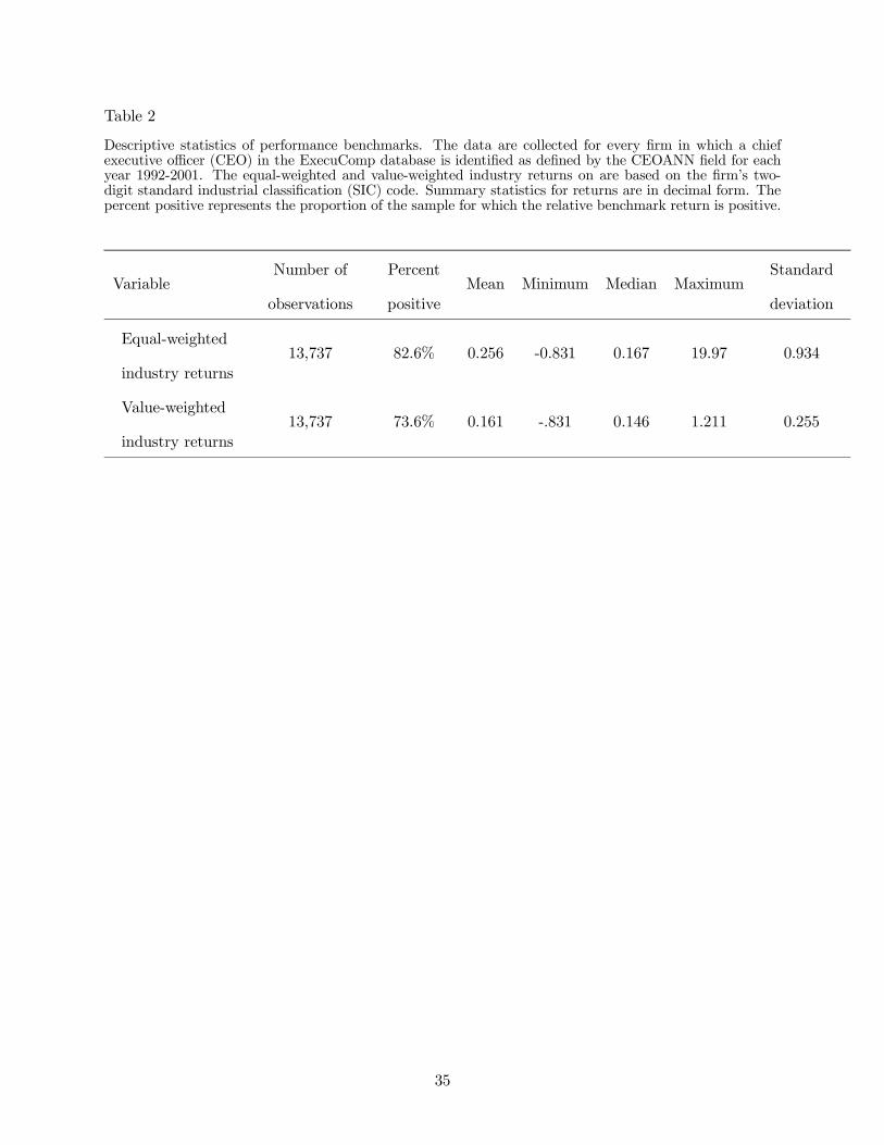
Table 2

Descriptive statistics of performance benchmarks. The data are collected for every firm in which a chiefexecutive officer (CEO) in the ExecuComp database is identified as defined by the CEOANN field for eachyear 1992-2001. The equal-weighted and value-weighted industry returns on are based on the firm’s two-digit standard industrial classification (SIC) code. Summary statistics for returns are in decimal form. Thepercent positive represents the proportion of the sample for which the relative benchmark return is positive.

VariableNumber of

observations

Percent

positiveMean Minimum Median Maximum

Standard

deviation

Equal-weighted

industry returns13,737 82.6% 0.256 -0.831 0.167 19.97 0.934

Value-weighted

industry returns13,737 73.6% 0.161 -.831 0.146 1.211 0.255

35

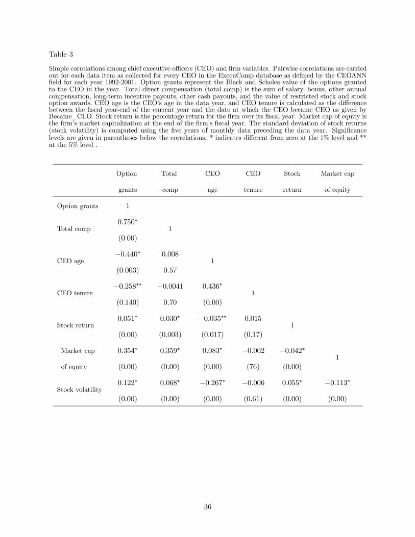
Table 3

Simple correlations among chief executive officers (CEO) and firm variables. Pairwise correlations are carriedout for each data item as collected for every CEO in the ExecuComp database as defined by the CEOANNfield for each year 1992-2001. Option grants represent the Black and Scholes value of the options grantedto the CEO in the year. Total direct compensation (total comp) is the sum of salary, bonus, other annualcompensation, long-term incentive payouts, other cash payouts, and the value of restricted stock and stockoption awards. CEO age is the CEO’s age in the data year, and CEO tenure is calculated as the differencebetween the fiscal year-end of the current year and the date at which the CEO became CEO as given byBecame_CEO. Stock return is the percentage return for the firm over its fiscal year. Market cap of equity isthe firm’s market capitalization at the end of the firm’s fiscal year. The standard deviation of stock returns(stock volatility) is computed using the five years of monthly data preceding the data year. Significancelevels are given in parentheses below the correlations. * indicates different from zero at the 1% level and **at the 5% level .

Option

grants

Total

comp

CEO

age

CEO

tenure

Stock

return

Market cap

of equity

Option grants 1

Total comp0.750∗

(0.00)

1

CEO age−0.440∗

(0.003)

0.008

0.57

1

CEO tenure−0.258∗∗

(0.140)

−0.00410.70

0.436∗

(0.00)

1

Stock return0.051∗

(0.00)

0.030∗

(0.003)

−0.035∗∗

(0.017)

0.015

(0.17)1

Market cap

of equity

0.354∗

(0.00)

0.359∗

(0.00)

0.083∗

(0.00)

−0.002(76)

−0.042∗

(0.00)1

Stock volatility0.122∗

(0.00)

0.068∗

(0.00)

−0.267∗

(0.00)

−0.006(0.61)

0.055∗

(0.00)

−0.113∗

(0.00)

36

Table 4

Column 1 of Panel A contains an ordinary least squares regression of changes in total direct chief executiveofficer compensation on the contribution of exogenous factors (luck) on the performance of the firm’s dollarreturns, the contribution of firm-specific performance, the cdf of the dollar variance of firm returns, tenure,and an interaction of luck with the cdf of the variance of luck and skill with the variance of skill, plusexecutive fixed effects and year effects. Column 2 replaces total compensation with bonus, and Column 3uses the Black and Scholes value of options granted. Total direct compensation is the sum of salary, bonus,other annual compensation, long-term incentive payouts, other cash payouts, and the value of restrictedstock and stock option awards. In the row labeled Pr (b = a), we provide the p-value from the test thatb− a = 0. Pr (b = a) is evaluated at the median for both variance of luck and skill. Robust standard errorsare reported in parentheses, and the coefficients on the intercept, the cdf of the dollar variance tenure, andthe year and executive fixed effects are suppressed for convenience. * indicates different from zero at the1% level, ** at the 5% level, and *** at the 10% level. In each case, there are 6,263 observations. PanelB contains summary statistics on the predicted dollar values of luck (λ) and the residual skill (ε) from ourfirst-stage regression of firm returns on equally-weighted and value-weighted average industry returns, whereindustry is given by the firm’s two-digit standard industrial classification code.

Panel A. Paying for luck

Independent variables Total compensation Bonus Option grants

(1) (2) (3)

Luck (λ)1.405∗

(0.463)

0.346∗

(0.058)

0.703∗∗

(0.352)

Skill (ε)1.823∗

(0.420)

0.598∗

(0.047)

0.842∗

(0.253)

Luck × cdf variance of luck−1.33∗

(0.438)

−0.334∗

(0.056)

−0.701∗∗

(0.357)

Skill × cdf variance of skill−1.725∗

(0.316)

−0.579∗

(0.050)

−0.844∗

(0.278)

R2 0.197 0.290 0.188

Pr(b = a) 0.47 0.018 0.67

Panel B. Summary statistics on luck and skill

Variable Mean 1% Median 99% Standard deviation

Luck (λ) 945.8 -2,944.4 154.7 17,124.1 3,884.0

Skill (ε) -159.9 -14,014.4 -35.4 11,030.5 4,329.2

37

Table 5

Testing for asymmetry around zero. Column 1 contains an ordinary least squares regression of changesin total direct chief executive officer compensation on the contribution of exogenous factors (luck) on theperformance of the firm’s dollar returns, the contribution of firm-specific performance, and interactions ofboth luck and skill with dummy variables indicating that luck or skill are negative. We also control for thecdf of the dollar variance of firm returns, tenure, and an interaction of luck with the cdf of the variance of luckand skill with the variance of skill, plus executive fixed effects and year effects. Column 2 estimates the samemodel, but drops the interaction of skill and the dummy variable indicating that skill is negative. Column 3estimates the same model as Column 1, but relies on a median regression. Using the same specification asin Column 1, Column 4 replaces total compensation with bonus and Column 5 uses the Black and Scholesvalue of options granted. Total direct compensation is the sum of salary, bonus, other annual compensation,long-term incentive payouts, other cash payouts, and the value of restricted stock and stock option awards.In the row labeled Pr (bD= aD), we provide the p-value from the test that bD−aD= 0. Median bad luckremoved for median firm is equal to the opposite of the coefficient on the luck×luck is down (bD), divided bythe sensitivity of pay to luck (coefficient b on λ) for a firm with the median riskiness of luck. Robust standarderrors are reported in parentheses, and the coefficients on the intercept, the cdf of the dollar variance, tenure,and the year and executive fixed effects are suppressed for convenience. * indicates different from zero at the1% level and ** at the 5% level. N/A stands for not applicable. In each case, there are 6,263 observations.

38

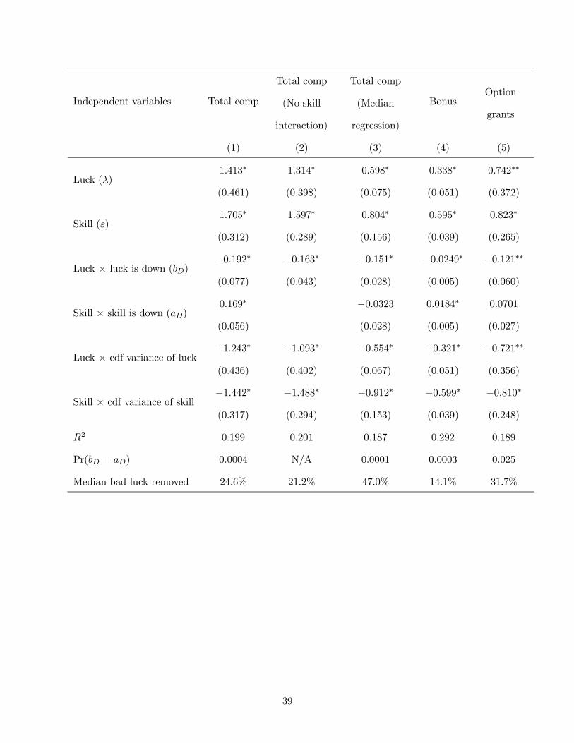
Independent variables Total comp

Total comp

(No skill

interaction)

Total comp

(Median

regression)

BonusOption

grants

(1) (2) (3) (4) (5)

Luck (λ)1.413∗

(0.461)

1.314∗

(0.398)

0.598∗

(0.075)

0.338∗

(0.051)

0.742∗∗

(0.372)

Skill (ε)1.705∗

(0.312)

1.597∗

(0.289)

0.804∗

(0.156)

0.595∗

(0.039)

0.823∗

(0.265)

Luck × luck is down (bD)−0.192∗

(0.077)

−0.163∗

(0.043)

−0.151∗

(0.028)

−0.0249∗

(0.005)

−0.121∗∗

(0.060)

Skill × skill is down (aD)0.169∗

(0.056)

−0.0323(0.028)

0.0184∗

(0.005)

0.0701

(0.027)

Luck × cdf variance of luck−1.243∗

(0.436)

−1.093∗

(0.402)

−0.554∗

(0.067)

−0.321∗

(0.051)

−0.721∗∗

(0.356)

Skill × cdf variance of skill−1.442∗

(0.317)

−1.488∗

(0.294)

−0.912∗

(0.153)

−0.599∗

(0.039)

−0.810∗

(0.248)

R2 0.199 0.201 0.187 0.292 0.189

Pr(bD = aD) 0.0004 N/A 0.0001 0.0003 0.025

Median bad luck removed 24.6% 21.2% 47.0% 14.1% 31.7%

39

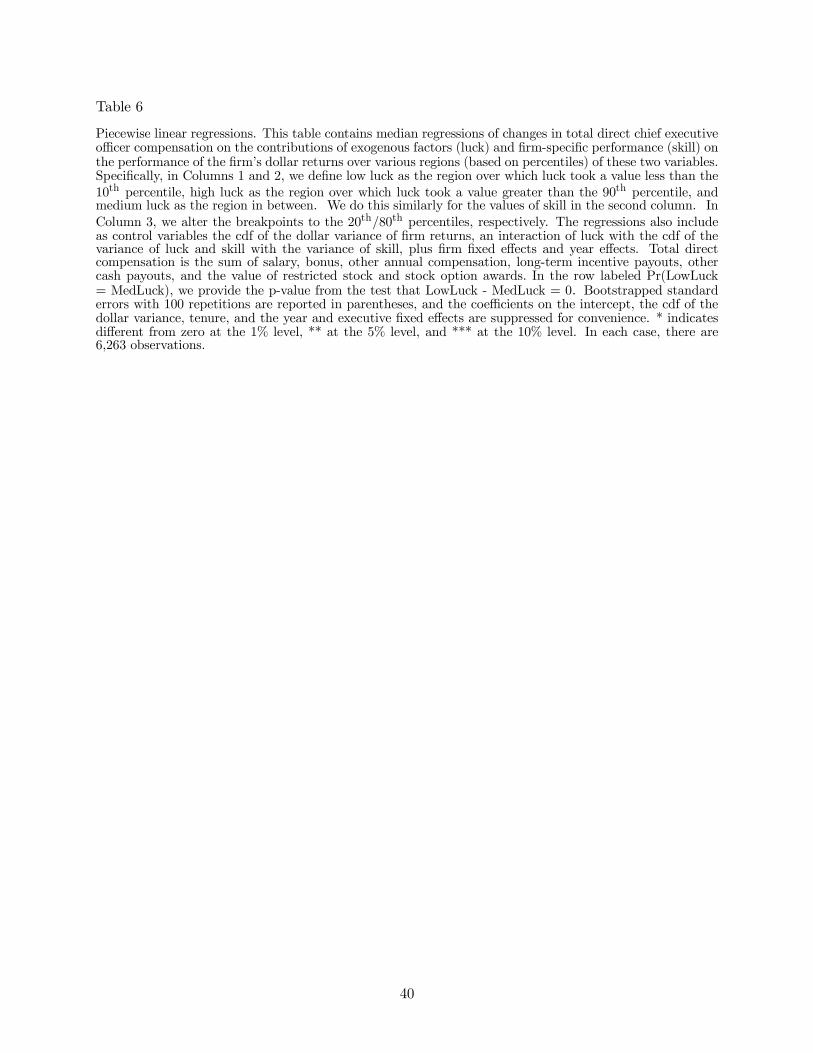
Table 6

Piecewise linear regressions. This table contains median regressions of changes in total direct chief executiveofficer compensation on the contributions of exogenous factors (luck) and firm-specific performance (skill) onthe performance of the firm’s dollar returns over various regions (based on percentiles) of these two variables.Specifically, in Columns 1 and 2, we define low luck as the region over which luck took a value less than the10th percentile, high luck as the region over which luck took a value greater than the 90th percentile, andmedium luck as the region in between. We do this similarly for the values of skill in the second column. InColumn 3, we alter the breakpoints to the 20th/80th percentiles, respectively. The regressions also includeas control variables the cdf of the dollar variance of firm returns, an interaction of luck with the cdf of thevariance of luck and skill with the variance of skill, plus firm fixed effects and year effects. Total directcompensation is the sum of salary, bonus, other annual compensation, long-term incentive payouts, othercash payouts, and the value of restricted stock and stock option awards. In the row labeled Pr(LowLuck= MedLuck), we provide the p-value from the test that LowLuck - MedLuck = 0. Bootstrapped standarderrors with 100 repetitions are reported in parentheses, and the coefficients on the intercept, the cdf of thedollar variance, tenure, and the year and executive fixed effects are suppressed for convenience. * indicatesdifferent from zero at the 1% level, ** at the 5% level, and *** at the 10% level. In each case, there are6,263 observations.

40

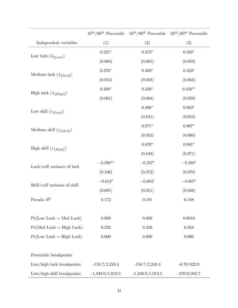
10th/90th Percentile 10th/90th Percentile 20th/80th Percentile

Independent variables (1) (2) (3)

Low luck (λ{Low})0.221∗

(0.060)

0.272∗

(0.065)

0.328∗

(0.059)

Medium luck (λ{Med})0.376∗

(0.054)

0.403∗

(0.058)

0.423∗

(0.064)

High luck (λ{High})0.389∗

(0.061)

0.420∗

(0.064)

0.458∗∗

(0.059)

Low skill (ε{Low})0.866∗

(0.041)

0.864∗

(0.053)

Medium skill (ε{Med})0.871∗

(0.052)

0.867∗

(0.060)

High skill (ε{High})0.870∗

(0.048)

0.981∗

(0.071)

Luck×cdf variance of luck−0.290∗∗

(0.106)

−0.337∗

(0.072)

−0.388∗

(0.070)

Skill×cdf variance of skill−0.612∗

(0.091)

−0.804∗

(0.051)

−0.807∗

(0.046)

Pseudo R2 0.172 0.191 0.188

Pr(Low Luck = Med Luck) 0.000 0.000 0.0016

Pr(Med Luck = High Luck) 0.532 0.429 0.358

Pr(Low Luck = High Luck) 0.000 0.000 0.000

Percentile breakpoints

Low/high luck breakpoints -158.7/2,243.4 -158.7/2,243.4 -6.70/822.9

Low/high skill breakpoints -1,349.0/1,013.5 -1,349.0/1,013.5 -470.9/282.7

41

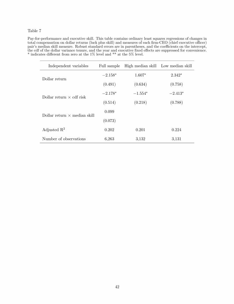
Table 7

Pay-for-performance and executive skill. This table contains ordinary least squares regressions of changes intotal compensation on dollar returns (luck plus skill) and measures of each firm-CEO (chief executive officer)pair’s median skill measure. Robust standard errors are in parentheses, and the coefficients on the intercept,the cdf of the dollar variance tenure, and the year and executive fixed effects are suppressed for convenience.* indicates different from zero at the 1% level and ** at the 5% level.

Independent variables Full sample High median skill Low median skill

Dollar return−2.158∗

(0.491)

1.607∗

(0.634)

2.342∗

(0.758)

Dollar return × cdf risk−2.178∗

(0.514)

−1.554∗

(0.218)

−2.413∗

(0.788)

Dollar return × median skill0.099

(0.073)

Adjusted R2 0.202 0.201 0.224

Number of observations 6,263 3,132 3,131

42

Table 8

Luck versus skill and CEO turnover. This table contains probit regressions of the probability the CEO leavesher firm in a given year. Age is a dummy variable that takes on the value one if the CEO is 65 years or older.Column 1 uses continuous measures of the contribution of exogenous factors (luck) on the performance ofthe firm’s dollar returns and the contribution of firm-specific performance (skill). Column 2 uses dummyvariables taking on the value one if the relevant measure is negative. In the row labeled Pr (b = a), weprovide the p-value from the test that b - a = 0. The estimated intercept term and coefficients on controlsfor market capitalization, asset value, and year dummies are suppressed for convenience. * indicates differentfrom zero at the 1% level and ** at the 5% level. In each case, there are 6,809 observations.

Continuous measures Dummy for bad luck and skill

(1) (2)

Luck−0.008(0.025)

Skill−0.0291∗

(0.011)

Luck is down−0.126(0.135)

Skill is down0.266∗∗

(0.115)

Age0.0210∗∗

(0.009)

0.202∗∗

(0.009)

Tenure−1.749∗

(0.254)

−1.651∗

(0.077)

Log likelihood -836 -877

Pr(b = a) 0.31 0.027

43

Table 9

Differential asymmetry based on governance index. Columns 1-5 of this table contain ordinary least squaresregressions of changes in total direct chief executive officer compensation on the contribution of exogenousfactors (luck) on the performance of the firm’s dollar returns, the contribution of firm-specific performance,the cdf of the dollar variance of firm returns, tenure, and interactions of luck with the cdf of the varianceof luck and skill with the variance of skill, plus industry fixed effects and year effects. Columns 1 and 3contain coefficient estimates for the subsample of firms in the bottom quintile (G ≤ 6) of the Gompers, Ishii,and Metrick (2003) Corporate Governance Index (strong governance). Columns 2 and 4 contain coefficientestimates for the subsample of firms in the top quintile (G ≥ 12) of the Corporate Governance Index (weakgovernance). Columns 3 and 4 include the interaction of luck with a dummy variable indicating whetherluck is negative. Column 5 contains estimates from the same model for the full sample but includes twoadditional interactions of luck with a dummy variable indicating whether luck is negative with anotherdummy variable indicating whether corporate governance is good (G ≤ 6) or poor (G ≥ 12). Here, wecan interpret the coefficient on luck with an indicator of whether luck is negative as capturing the firmsof intermediate governance quality. Total direct compensation is the sum of salary, bonus, other annualcompensation, long-term incentive payouts, other cash payouts, and the value of restricted stock and stockoption awards. Robust standard errors are reported in parentheses, and the coefficients on the intercept, thecdf of the dollar variance, tenure, and the year and industry fixed effects are suppressed for convenience. *indicates different from zero at the 1% level, ** at the 5% level, and *** at the 10% level.

44

Strong

governance

G ≤ 6

Weak

governance

G ≥ 12

Strong

governance

G ≤ 6

Weak

governance

G ≥ 12

Full

sample

Independent variables (1) (2) (3) (4) (5)

Luck (λ)1.91∗∗∗

(1.02)

2.45∗

(0.719)

1.56

(1.03)

2.81∗

(0.735)

1.28∗

(0.382)

Skill (ε)2.77∗

(0.765)

1.44∗

(0.493)

2.83∗

(0.765)

1.46∗

(0.492)

1.60∗

(0.264)

Luck × luck is down (bD)0.312∗∗∗

(0.165)

−0.364∗∗

(0.161)

−0.238∗

(0.076)

Luck × luck is down ×strong governance{G≤6}

0.44∗

(0.149)

Luck × luck is down ×weak governance{G≥12}

−0.021(0.170)

Luck × cdf variance of luck−1.90∗∗∗

(1.038)

−2.34∗

(0.737)

−1.584(1.051)

−2.67∗

(0.750)

−1.22∗

(0.388)

Skill × cdf variance of skill−2.93∗

(0.795)

−1.30∗∗

(0.510)

−3.00∗

(0.795)

−1.32∗

(0.510)

−1.55∗

(0.272)

Number of observations 944 1,146 944 1,146 5,377

R2 0.061 0.106 0.065 0.110 0.026

Pr(StrongGov = IntermGov) 0.0009

Pr(StrongGov = WeakGov) 0.4681

Pr(IntermGov = WeakGov) 0.0254

45

Table 10

Option granting policies and luck. The dependent variable in all cases is the Black and Scholes value ofoptions granted. Lagged option grants is the value of options granted in the previous year. Robust standarderrors are in parentheses, and the coefficients on the control variables (risk, luck, skill, luck and skill interactedwith the cdf of risk, asset value, market capitalization, debt/assets, tenure, and year and two-digit standardindustrial classification dummies) are suppressed for convenience. * indicates different from zero at the 1%level, ** at the 5% level, and *** at the 10% level. N/A stands for not applicable. In each case, there are6,263 observations.

Value of options granted

Independent variables

Lagged option grant0.349∗

(0.013)

0.353∗

(0.020)

0.337∗

(0.015)

Lagged option grant × luck is down (bD)0.0411∗∗

(0.021)

0.0439∗∗

(0.0201)

Lagged option grant × skill is down (aD)−0.0437∗∗∗

(0.023)

Adjusted R2 0.337 0.339 0.338

Pr(bD = aD) NA 0.0058 NA

46

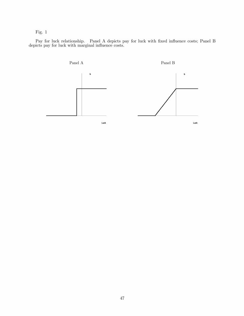
Fig. 1

Pay for luck relationship. Panel A depicts pay for luck with fixed influence costs; Panel Bdepicts pay for luck with marginal influence costs.

Panel A Panel B

Luck

b

Luck

b

Luck

b

Luck

b

47

Fig. 2

Asymmetric performance: Panel A depicts the realizations of luck and skill, while Panel Bdepicts the implied pay for luck relationship that would be estimated.

Panel A Panel B

f’s skill

f’s luck = i’s luck = - i’s skill

1 - 1

1

½

- ½

- 1

i’s skill

f’s luck = i’s luck = - f’s skill

Estimated Relationship •

•

½

- ½

f

f/2

- i/2

- i i’s pay when luck is bad •

i’s pay when luck is good

f’s pay when luck is good

f’s pay when luck is bad

•

48