Astronomy - USPmaciel/research/articles/art91.pdf · 2 Department of Astronomy, Odessa State...

A&A 381, 32–50 (2002)DOI: 10.1051/0004-6361:20011488c© ESO 2002

Astronomy&

Astrophysics

Using Cepheids to determine the galactic abundance gradient

I. The solar neighbourhood ?,??

S. M. Andrievsky1,2, V. V. Kovtyukh2,3, R. E. Luck4,5, J. R. D. Lepine1,D. Bersier6, W. J. Maciel1, B. Barbuy1, V. G. Klochkova7,8, V. E. Panchuk7,8, and R. U. Karpischek9

1 Instituto Astronomico e Geofısico, Universidade de Sao Paulo, Av. Miguel Stefano, 4200 Sao Paulo SP, Brazile-mail: [email protected]

2 Department of Astronomy, Odessa State University, Shevchenko Park, 65014, Odessa, Ukrainee-mail: [email protected]

3 Odessa Astronomical Observatory and Isaac Newton Institute of Chile, Odessa Branch, Ukraine4 Department of Astronomy, Case Western Reserve University, 10900 Euclid Avenue, Cleveland, OH 44106-7215,

USA, e-mail: [email protected] Visiting Astronomer, Cerro Tololo Inter-American Observatory, National Optical Astronomy Observatories

which are operated by the Association of Universities for Research in Astronomy, Inc., under contract with theUS National Science Foundation

6 Harvard-Smithsonian Center for Astrophysics, 60 Garden Street, MS 16, Cambridge, MA 02138, USAe-mail: [email protected]

7 Special Astrophysical Observatory, Russian Academy of Sciences, Nizhny Arkhyz, Stavropol Territory, 369167,Russiae-mail: [email protected]; [email protected]

8 SAO RAS and Isaac Newton Institute of Chile, SAO RAS Branch, Russia9 EdIC group, Universidade de Sao Paulo, Sao Paulo, Brazil

e-mail: [email protected]

Received 31 July 2001 / Accepted 10 October 2001

Abstract. A number of studies of abundance gradients in the galactic disk have been performed in recent years.The results obtained are rather disparate: from no detectable gradient to a rather significant slope of about−0.1 dex kpc−1. The present study concerns the abundance gradient based on the spectroscopic analysis ofa sample of classical Cepheids. These stars enable one to obtain reliable abundances of a variety of chemicalelements. Additionally, they have well determined distances which allow an accurate determination of abundancedistributions in the galactic disc. Using 236 high resolution spectra of 77 galactic Cepheids, the radial elementaldistribution in the galactic disc between galactocentric distances in the range 6–11 kpc has been investigated.Gradients for 25 chemical elements (from carbon to gadolinium) are derived. The following results were obtainedin this study. Almost all investigated elements show rather flat abundance distributions in the middle part ofgalactic disc. Typical values for iron-group elements lie within an interval from ≈−0.02 to ≈−0.04 dex kpc−1 (inparticular, for iron we obtained d[Fe/H]/dRG = −0.029 dex kpc−1). Similar gradients were also obtained for O,Mg, Al, Si, and Ca. For sulphur we have found a steeper gradient (−0.05 dex kpc−1). For elements from Zr to Gdwe obtained (within the error bars) a near to zero gradient value. This result is reported for the first time. Thoseelements whose abundance is not expected to be altered during the early stellar evolution (e.g. the iron-groupelements) show at the solar galactocentric distance [El/H] values which are essentially solar. Therefore, there isno apparent reason to consider our Sun as a metal-rich star. The gradient values obtained in the present studyindicate that the radial abundance distribution within 6–11 kpc is quite homogeneous, and this result favors agalactic model including a bar structure which may induce radial flows in the disc, and thus may be responsiblefor abundance homogenization.

Key words. stars: abundances – stars: supergiants – galaxy: abundances – galaxy: evolution

Send offprint requests to: S. M. Andrievsky,e-mail: [email protected]? Based on spectra collected at McDonald – USA, SAORAS

– Russia, KPNO – USA, CTIO – Chile, MSO – Australia, OHP– France.?? Full Table 1 is only available in electronic form athttp://www.edpsciences.org

Table A1 (Appendix) is only, and Table 2 also, avail-able in electronic form at the CDS via anonymous ftp tocdsarc.u-strasbg.fr (130.79.128.5)

or viahttp://cdsweb.u-strasbg.fr/cgi-bin/qcat?J/A+A/381/32

S. M. Andrievsky et al.: Galactic abundance gradient. I. 33

1. Introduction

In recent years the problem of radial abundance gradi-ents in spiral galaxies has emerged as a central problemin the field of galactic chemodynamics. Abundance gradi-ents as observational characteristics of the galactic disc areamong the most important input parameters in any the-ory of galactic chemical evolution. Further development oftheories of galactic chemodynamics is dramatically ham-pered by the scarcity of observational data, their largeuncertainties and, in some cases, apparent contradictionsbetween independent observational results. Many ques-tions concerning the present-day abundance distributionin the galactic disc, its spatial properties, and evolutionwith time, still have to be answered.

Discussions of the galactic abundance gradient, as de-termined from several studies, were provided by Friel(1995), Gummersbach et al. (1998), Hou et al. (2000).Here we only briefly summarize some of the more per-tinent results.

1) A variety of objects (planetary nebulae, cool gi-ants/supergiants, F-G dwarfs, old open clusters) seem togive evidence that an abundance gradient exists. UsingDDO, Washington, UBV photometry and moderate res-olution spectroscopy combined with metallicity calibra-tions for open clusters and cool giants the following gra-dients were derived (d[Fe/H]/dRG): −0.05 dex kpc−1

(Janes 1979), −0.095 dex kpc−1 (Panagia & Tosi 1981),−0.07 dex kpc−1 (Harris 1981), −0.11 dex kpc−1

(Cameron 1985), −0.017 dex kpc−1 (Neese & Yoss 1988),−0.13 dex kpc−1 (Geisler et al. 1992), −0.097 dex kpc−1

(Thogersen et al. 1993), −0.09 dex kpc−1 (Friel & Janes1993), −0.091 dex kpc−1 (Friel 1995), −0.09 dex kpc−1

(Carraro et al. 1998), −0.06 dex kpc−1 (Friel 1999; Phelps2000). One must also add that there have been attempts toderive the abundance gradient (specifically d[Fe/H]/dRG)using high-resolution spectroscopy of cool giant and su-pergiant stars. Harris & Pilachowski (1984) obtained−0.07 dex kpc−1, while Luck (1982) found a steeper gra-dient of −0.13 dex kpc−1.

Oxygen and sulphur gradients determined from ob-servations of planetary nebulae are −0.058 dex kpc−1

and −0.077 dex kpc−1 respectively (Maciel & Quireza1999), with slightly flatter values for neon and argon,as in Maciel & Koppen (1994). A smaller slope wasfound in an earlier study of Pasquali & Perinotto (1993).According to those authors the nitrogen abundance gra-dient is −0.052 dex kpc−1, while that of oxygen is−0.030 dex kpc−1.

2) From young B main sequence stars, Smartt &Rolleston (1997) found a gradient of −0.07 dex kpc−1,while Gehren et al. (1985), Fitzsimmons et al.(1992), Kaufer et al. (1994) and Kilian-Montenbrucket al. (1994) derived significantly smaller values:−0.03−0.00 dex kpc−1. No systematic abundancevariation with galactocentric distance was found byFitzsimmons et al. (1990). The recent studies ofGummersbach et al. (1998) and Rolleston et al. (2000)

support the existence of a gradient (−0.07 dex kpc−1).The elements in these studies were C-N-O and Mg-Al-Si.

3) Studies of the abundance gradient (primarily nitro-gen, oxygen, sulphur) in the Galactic disc based on youngobjects such as H ii regions give positive results: either sig-nificant slopes from −0.07 to −0.11 dex kpc−1 accordingto: Shaver et al. (1983) for nitrogen and oxygen, Simpsonet al. (1995) for nitrogen and sulphur, Afflerbach et al.(1997) for nitrogen, Rudolph et al. (1997) for nitrogenand sulphur, or intermediate gradients of about −0.05 to−0.06 dex kpc−1 according to: Simpson & Rubin (1990)for sulphur, Afflerbach et al. (1997) for oxygen and sul-phur; and negative ones: weak or nonexistent gradientsas concluded by Fich & Silkey (1991); Vilchez & Esteban(1996), Rodriguez (1999). Recently Pena et al. (2000) de-rived oxygen abundances in several H ii regions and founda rather flat distribution with galactocentric distance (co-efficient −0.04 dex kpc−1). The same results were alsoreported by Deharveng et al. (2000).

As one can see, there is no conclusive argument allow-ing one to come to a definite conclusion about whether ornot a significant abundance gradient exists in the galac-tic disc, at least for all elements considered and withinthe whole observed interval of galactocentric distances.Compared to other objects supplying us with an informa-tion about the radial distribution of elemental abundancesin the galactic disc, Cepheids have several advantages:

1) they are primary distance calibrators which provideexcellent distance estimates;

2) they are luminous stars allowing one to probe to largedistances;

3) the abundances of many chemical elements can bemeasured from Cepheid spectra (many more than fromH ii regions or B stars). This is important for investi-gation of the distribution in the galactic disc of abso-lute abundances and abundance ratios. Additionally,Cepheids allow the study of abundances past the iron-peak which are not generally available in H ii regionsor B stars;

4) lines in Cepheid spectra are sharp and well-definedwhich enables one to derive elemental abundances withhigh reliability.

In view of the inconsistencies in the current results on thegalactic abundance gradient, and those advantages whichare afforded by Cepheids, we have undertaken a large sur-vey of Cepheids in order to provide independent infor-mation which should be useful as boundary conditions fortheories of galactic chemodynamics. We also hope that theresults on the abundance gradient from the Cepheids willalso be helpful to constrain the structure and age of thebar, and its influence on the metallicity gradient. This firstpaper in this series on abundance gradients from Cepheidspresents the results for the solar neighbourhood.

34 S. M. Andrievsky et al.: Galactic abundance gradient. I.

2. Observations

For the great majority of the program stars multiphaseobservations were obtained. From the total number of thespectra for each star we selected those showing no or atmost a small asymmetry of the spectral lines. For the dis-tant (fainter) Cepheids we have analyzed 3–4 spectra inorder to derive the abundances, while for the nearby stars2–3 spectra were used. This is predicated on the fact thatthe brighter stars have higher S/N spectra and thus bet-ter determined equivalent widths. For some stars we haveonly one spectrum, and for a few Cepheids more than fourspectra were analyzed.

Information about the program stars and spectra isgiven in Table 1. Note that we also added to our sampletwo distant Cepheids (TV Cam and YZ Aur) which werepreviously analyzed by Harris & Pilachowski (1984). Wehave used their data for these stars but atmospheric pa-rameters and elemental abundances (specifically the ironcontent) were re-determined using the same methodologyas for other program stars (see next section).

3. Methodology

3.1. Line equivalent widths

The line equivalent widths in the Cepheid spectra weremeasured using the Gaussian approximation, or in somecases, by direct integration. To estimate the internalaccuracy of the measurements we have compared theequivalent widths of lines present in adjacent overlappingechelle orders. In no case did the difference between in-dependent estimates exceed 10%. The measured equiv-alent widths were analyzed in the LTE approximationusing the WIDTH9 code of Kurucz. Only lines havingWλ ≤ 165 mA were used for abundance determination.The total number of lines used in the analysis exceeds41 000.

3.2. Atmosphere models

Plane-parallel LTE atmosphere models (ATLAS9) fromKurucz (1992) were used to determine the elemental abun-dances. Final models were interpolated (in Teff and log g)from the solar metallicity grid computed using a microtur-bulent velocity of 4 km s−1. The adopted microturbulentvelocities vary from 3 to 8 km s−1 but numerical experi-ment shows that the derived abundances are not substan-tially altered by the mismatch between the model micro-turbulence and the value used to compute the abundances.Note that the ATLAS9 models are in a regime where theconvection problem discovered by Castelli (1996) does notcause a significant problem.

3.3. Oscillator strengths and damping constants

The oscillator strengths used in present study were ob-tained through an inverted solar analysis (with elemental

abundances adopted following Grevesse et al. 1996). Theywere derived using selected unblended solar lines from thesolar spectrum by Kurucz et al. (1984). A detailed descrip-tion and list of the log gf values can be found in Kovtyukh& Andrievsky (1999). The damping constants for the linesof interest were taken from the list of B. Bell. It is wellknown that the classical treatment of the van der Waalsbroadening leads to broadening coefficients which are toosmall (see Barklem et al. 2000).

3.4. Stellar parameters

The effective temperature for each program star was deter-mined using the method described in detail in Kovtyukh& Gorlova (2000). That method is based on the use of re-lations between effective temperature and the line depthratios (each ratio is for the weak lines with different exci-tation potentials of the same chemical element). The ad-vantages of this method are the following: such ratios aresensitive to the temperature variations, they do not de-pend upon the abundances and interstellar reddening. Themain source of initial temperatures used for the calibrat-ing relations was Fry & Carney (1997). Their data are ingood agreement with the results obtained by other meth-ods, such as the infrared flux method (Fernley et al. 1989)or detailed analysis of energy distribution (Evans & Teays1996). Another source was photometry (Kiss 1998).

The number of temperature indicators (ratios) is typ-ically 30. The precision of the Teff determination is 10–30 K (standard error of the mean) from the spectra withS/N greater than 100, and 30–50K for S/N less than 100.Although an internal error of Teff determination appearsto be small, a systematic shift of the zero-point of Teff scalemay exist. Nevertheless, an uncertainty in the zero-point(if it exists) can affect absolute abundances in each pro-gram star, but the slopes of the abundance distributionsshould be hardly affected.

The microturbulent velocity and gravity were foundusing the technique put forth by Kovtyukh & Andrievsky(1999). This method was applied to an investigation ofLMC F supergiants with well known distances, and itproduced much more appropriate gravities for those starsthan were previously determined (see Hill et al. 1995). Themethod also allowed to solve several problems connectedwith abundances in the Magellanic Cloud supergiants (fordetails see Andrievsky et al. 2001). Results on Teff , log gand Vt determination are gathered in Table 1 (the quotedprecision of the Teff values presented in Table 1 is not rep-resentative of the true precision which is stated above).

Several remarks on the gravity results for our programCepheids have to be made. It is expected that the gravi-ties of Cepheids, being averaged over the pulsational cycle,should correlate with their pulsational periods in the sensethat lower gravities correspond to larger periods. As it wasanalytically shown by Gough et al. (1965), the pulsationalperiod P behaves as P ∼ R2M−1, i.e. ∼g−1 (where R,M and g are the radius, mass and gravity of a Cepheid


Table 1. Program Cepheids, their spectra and results for individual phases.

Star P, d JD, 24+ φ Telescope Teff , K log g Vt, km s−1 [Fe/H]

V473 Lyr (s) 1.4908 49906.43160 0.793 OHP 1.93 m 6163 2.45 4.20 –0.0949907.57360 0.559 OHP 1.93 m 6113 2.60 4.50 –0.05

SU Cas(s) 1.9493 50674.95633 0.902 MDO 2.1 m 6594 2.60 3.85 –0.0250675.96550 0.420 MDO 2.1 m 6162 2.25 3.00 –0.0050678.93059 0.941 MDO 2.1 m 6603 2.50 3.50 –0.0151473.79052 0.704 MDO 2.1 m 6201 2.30 2.85 –0.00

EU Tau (s) 2.1025 51096.90943 0.172 MDO 2.1 m 6203 2.00 3.00 –0.0951097.89587 0.641 MDO 2.1 m 6014 2.20 3.30 –0.03

IR Cep (s) 2.1140 48821.46940 0.137 SAORAS 6 m 6162 2.40 4.10 +0.00

respectively). A similar relation between pulsational pe-riod and gravity can be also derived, for example, by com-bining observational “period-mass” and “period-radius”relations established for Cepheids by Turner (1996) andGieren et al. (1998) respectively.

As for each star of our sample we have only a lim-ited number of the gravity estimates, in Fig. 1 we simplyplotted individual log g (gravity in cm s−2) values for agiven Cepheid versus its pulsational period of the funda-mental mode (period is given in days). The general trendcan be clearly traced from this figure. For the long-periodCepheids the scatter in the gravities derived at the dif-ferent pulsational phases achieves approximately 1 dex.The instantaneous gravity value, in fact, is a combina-tion of the static component GM/R2 and dynamical termγ dV /dt (γ is the projection factor and V is the radial ve-locity). This means that observed amplitudes of the grav-ity variation do not reflect purely pulsational changes ofthe Cepheid radius. Nevertheless, there may exist some ad-ditional mechanism artificially “lowering” gravities whichare derived through spectroscopic analysis, and thus in-creasing an amplitude of the gravity variation. Such effectsas, for example, sphericity of the Cepheid atmospheres,additional UV flux and connected with it an overion-ization of some elements, stellar winds and mass loss,rotation and macroturbulence, may contribute to someincrease of the spectroscopic gravity variation over a pul-sational cycle. It is quite likely that these effects shouldbe more pronounced in the more luminous (long-period)Cepheids, and they may affect the abundances resultingfrom the gravity sensitive ionized species. To investigatethis problem one needs to perform a special detailed mul-tiphase analysis for Cepheids with various pulsational pe-riods. From our sample of stars only for TU Cas, U Sgrand SV Vul we have enough data to observe effects.

In Figs. 2–3 we plotted Ce and Eu abundances togetherwith spectroscopic gravities versus pulsational phases forthe intermediate-period Cepheid U Sgr (P ≈ 7 days) andfor SV Vul (P ≈ 45 days), one of the longest periodCepheid among our program stars. A scatter of about0.15 dex is seen for both elements which are presented inthe spectra only by ionized species. Inspecting Fig. 3 onemight suspect some small decrease of abundances aroundphase 0.4 (roughly corresponds to a maximum in SV Vulradius). It can be attributed to NLTE effects, which shouldincrease in the extended spherical atmosphere of lower

density. More precisely, a small decrease in the abundancesmay be caused by additional overionization of the dis-cussed ions having rather low ionization potentials (about11 eV). Although the s-process elements in Cepheids aremeasured primarily by ionized species, and any errors inthe stellar gravities at some phases propagate directly intothe abundance results, we do not think that this effectmay have some radical systematic influence on abundanceresults for the s-process elements in our program stars.The reasons are the following. An indicated decrease inthe abundance is rather small, even for the long-periodCepheid, and practically is not seen for shorter periods.In fact, a decrease of about 0.15 dex is comparable witherrors in the abundance determination for the elementswith small number of lines, like s-process elements. Onecan also add that the abundances averaged from differentphases should be sensitive to this effect even to a lesserextent.

4. Elemental abundances

Detailed abundance results are presented in the Appendix(Table A1) and Table 2. The Appendix contains the perspecies abundances averaged over all individual spectra(phases) for each star along with the total number of linesand standard deviation. Table 2 contains the final aver-aged abundance per element. The latter abundances wereobtained by averaging all lines from all ions at all phases:that is, for example a sum of all iron line abundances fromall phases and divide by the total number of lines. The ironabundance for individual phases is presented in Table 1,and the mean iron abundance for each star is also repeatedin Table 3. Note that standard deviation of the abundanceof an element falls within the range 0.05–0.20 dex for alldeterminations. Because the number of lines used for someelements is large (especially for iron), the standard errorof the mean abundance is very small.

Note that the modified method of LTE spectroscopicanalysis described in Kovtyukh & Andrievsky (1999) spec-ifies the microturbulent velocity as a fitting parameter toavoid any systematic trend in the “[Fe/H]−EW” relationbased on Fe ii lines (which are not significantly affected byNLTE effects unlike Fe i lines which may be adversely af-fected). With the microturbulent velocity obtained in thisway, the Fe i lines demonstrate a progressively decreas-ing iron abundance as a function of increasing equivalent


Fig. 1. Program Cepheid gravities vs. their pulsational periods.

Fig. 2. Relative-to-solar Ce and Eu abundance and spectro-scopic gravity of U Sgr vs. its pulsational phases.

width. Kovtyukh & Andrievsky (1999) attribute this be-havior to departures from LTE in Fe i. To determine the

Fig. 3. Same as Fig. 2 but for SV Vul.

true iron abundance from Fe i lines one refers the abun-dance to the lowest EW, and it is therefore determinedusing the [Fe/H]−EW relation for these lines (and this


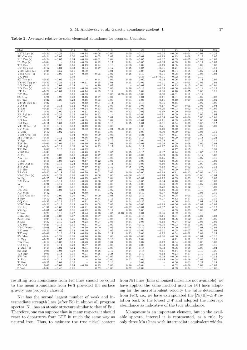
Table 2. Averaged relative-to-solar elemental abundance for program Cepheids.

Star C O Na Mg Al Si S Ca Sc Ti V Cr Mn

V473 Lyr (s) −0.34 −0.24 0.01 −0.14 −0.06 −0.03 0.09 −0.10 −0.05 −0.06 −0.04 −0.08 −0.22SU Cas (s) −0.24 −0.02 0.20 −0.24 0.05 0.07 0.11 −0.01 −0.13 0.13 0.08 0.12 0.07EU Tau (s) −0.24 −0.05 0.24 −0.28 −0.01 0.04 0.09 −0.05 −0.07 0.03 −0.05 −0.02 −0.05IR Cep (s) −0.04 – 0.28 −0.39 0.12 0.17 0.34 −0.06 −0.03 0.09 0.26 −0.12 −0.02TU Cas −0.19 −0.03 0.15 −0.19 0.14 0.10 −0.03 −0.02 −0.19 0.05 0.02 0.02 0.06DT Cyg (s) −0.12 0.01 0.33 0.04 0.17 0.12 0.15 0.05 −0.01 0.21 0.14 0.18 0.19V526 Mon (s) −0.28 −0.52 0.11 −0.09 – −0.01 0.05 −0.08 −0.20 −0.04 −0.18 −0.02 −0.14V351 Cep (s) −0.19 −0.09 0.17 −0.30 −0.03 0.07 0.26 −0.10 0.01 0.08 0.08 0.03 −0.03VX Pup – – 0.08 – – −0.06 – −0.33 −0.13−0.01 −0.02 −0.16 −0.10SZ Tau (s) −0.20 −0.02 0.25 – 0.14 0.07 0.19 0.02 0.02 0.06 0.10 0.18 0.09V1334 Cyg (s) −0.30 −0.23 0.18 −0.31 0.15 0.08 0.11 −0.03 −0.01 0.02 −0.01 −0.03 0.03BG Cru (s) −0.18 0.08 0.24 – 0.29 0.07 – −0.01 −0.33 0.13 0.15 −0.04 −0.01BD Cas (s) −0.14 −0.09 −0.03 −0.26 −0.09 0.03 0.26 −0.19 −0.23 −0.06 −0.06 −0.14 −0.13RT Aur −0.22 −0.01 0.29 −0.14 0.13 0.12 0.19 0.09 0.05 0.10 0.05 0.08 0.11DF Cas −0.30 – 0.16 −0.33 – 0.03 0.39−0.18 −0.09 0.00 −0.01 0.11 −0.12SU Cyg −0.21 −0.25 0.23 −0.16 0.17 0.04 0.02 0.01 −0.11 0.01 0.06 0.02 0.02ST Tau −0.27 −0.29 0.23 −0.18 0.03 0.03 0.04 −0.04 −0.11 0.10 −0.07 −0.04 −0.02V1726 Cyg (s) −0.22 – 0.29 −0.12 0.07 0.11 0.17 −0.16 −0.05 0.15 – −0.07 0.00BQ Ser −0.15 −0.13 0.12 −0.14 0.14 0.07 0.13 −0.05 −0.17 0.03 −0.01 0.04 −0.04Y Lac −0.26 −0.37 0.13 −0.24 0.13 0.03 −0.04 −0.05 −0.26 −0.03 0.02 −0.07 −0.09T Vul −0.26 0.00 0.13 −0.31 0.12 0.04 0.12 0.03 −0.19 0.00 0.00 0.10 0.01FF Aql (s) −0.31 −0.23 0.25 −0.24 0.12 – 0.01 −0.03 −0.11 0.09 0.14 0.06 0.04CF Cas −0.19 0.06 0.09 −0.21 0.10 0.01 0.10 −0.01 −0.04 −0.00 −0.06 0.06 −0.01BG Lac −0.17 0.10 0.17 −0.25 0.08 0.04 0.09 −0.01 −0.11 0.03 −0.05 0.06 0.04Del Cep −0.17 0.01 0.20 −0.16 0.16 0.10 0.15 0.01 0.01 0.04 0.09 0.06 0.17V1162 Aql (s) −0.14 −0.19 0.13 −0.19 0.13 0.06 – −0.03 −0.21 −0.03 −0.02 0.02 −0.01CV Mon −0.25 0.02 0.03 −0.32 −0.05 0.01 0.08−0.19 −0.14 0.10 0.30 0.04 −0.05V Cen −0.17 0.02 0.01 – 0.11 0.03 0.14 −0.03 0.00 0.09 0.03 −0.04 −0.11V924 Cyg (s:) −0.30 – −0.04 −0.38 0.09 −0.04 0.05 −0.21 −0.37 −0.21 0.01 −0.09 0.10MY Pup (s) −0.36 −0.12 0.14 −0.36 0.03 −0.08 −0.14 −0.13 −0.17 −0.09 −0.09 −0.18 −0.24Y Sgr −0.14 −0.06 0.22 −0.03 0.27 0.12 0.17 0.04 −0.24 0.01 0.07 0.17 0.11EW Sct −0.07 −0.04 0.07 −0.10 0.15 0.08 0.15 −0.01 −0.09 0.09 0.08 0.05 0.08FM Aql −0.24 −0.19 0.32 0.00 0.33 0.17 0.24 0.17 −0.17 0.15 0.10 0.19 0.11TX Del 0.06 0.16 0.48 −0.22 – – – 0.16 – 0.17 0.15 – 0.38V367 Sct −0.38 – 0.21 −0.48 0.21 0.05 0.15 −0.15 0.07 0.24 0.06 −0.05 −0.13X Vul −0.16 0.03 0.18 −0.20 0.17 0.08 0.20 −0.04 −0.09 0.08 0.04 0.12 0.08AW Per −0.23 −0.03 0.24 −0.27 0.07 0.06 0.18 −0.03 −0.15 0.01 0.15 0.27 0.10U Sgr −0.16 0.03 0.20 −0.17 0.22 0.07 0.15 0.03 −0.16 0.06 0.03 0.10 0.06V496 Aql (s) −0.20 −0.15 0.24 −0.12 0.10 0.11 0.13 −0.03 0.10 0.06 0.06 0.09 0.05Eta Aql −0.20 −0.10 0.19 −0.19 0.23 0.12 0.08 −0.02 −0.18 0.03 0.02 0.22 0.12BB Her −0.10 0.04 0.40 −0.01 0.23 0.15 – −0.01 0.07 0.09 0.07 0.10 0.30RS Ori −0.45 −0.18 0.06 −0.30 0.02 0.02 0.00 −0.06 −0.19 0.11 −0.12 −0.09 −-0.11V440 Per (s) −0.34 −0.21 0.05 −0.33 0.06 0.00 −0.06 −0.16 −0.14 0.05 0.00 –0.06 –0.04W Sgr −0.25 0.02 0.18 −0.25 −0.01 0.04 0.11 −0.01 −0.12 0.03 0.03 0.03 0.03RX Cam −0.25 −0.11 0.18 −0.23 0.06 0.05 0.04 −0.05 0.04 0.10 0.03 0.08 0.02W −0.27 −0.12 0.18 −0.28 0.10 0.03 0.05 −0.08 0.05 0.09 0.00 −0.02 −0.02U Vul −0.18 −0.03 0.18 −0.16 0.12 0.09 0.17 −0.05 −0.28 0.05 0.02 0.10 0.01DL Cas −0.31 −0.01 0.11 0.11 0.14 0.02 0.21 0.01 −0.16 0.03 −0.04 0.10 0.07AC Mon −0.42 – 0.24 −0.40 – −0.02 −0.15 −0.10 −0.07 0.12 – −0.08 −0.19V636 Cas (s) −0.17 −0.09 0.29 −0.07 0.09 0.08 0.12 0.15 0.25 0.05 0.05 0.30 0.10S Sge −0.12 0.04 0.24 −0.22 0.14 0.16 0.17 0.03 0.27 0.12 0.17 0.22 0.19GQ Ori −0.37 −0.12 0.17 0.11 0.04 0.00 0.04 −0.25 – 0.06 0.04 0.01 −0.14V500 Sco −0.20 −0.13 0.13 −0.23 0.08 0.02 0.06 −0.09 −0.13 −0.06 −0.10 −0.07 −0.03FN Aql −1.31 −0.08 0.19 −0.21 0.10 0.00 −0.02 −0.07 −0.07 0.04 0.01 −0.04 −0.12YZ Sgr −0.07 −0.07 0.31 −0.22 0.18 0.12 0.18 0.00 – 0.03 0.03 0.09 0.07S Nor −0.23 −0.19 0.27 −0.24 0.16 0.05 0.10−0.03 0.01 0.05 0.02 −0.08 −0.10Beta Dor −0.31 −0.08 0.07 −0.30 0.07 0.00 −0.04 −0.18 −0.11 0.01 −0.05 −0.04 0.03Zeta Gem −0.24 −0.12 0.25 −0.15 0.07 0.04 0.03 −0.06 0.13 0.06 0.02 0.00 0.05Z Lac −0.32 −0.10 0.23 −0.23 0.07 0.05 0.14 0.04 −0.18 0.07 −0.02 0.05 0.05VX Per −0.25 −0.15 0.15 −0.31 0.03 0.00 0.04 −0.12 −0.05 −0.03 −0.11 −0.06 −0.09V340 Nor(s:) −0.08 0.07 0.29 −0.30 0.00 0.03 0.18 −0.16 −0.12 0.00 −0.07 0.01 −0.03RX Aur −0.29 −0.02 0.18 −0.20 0.04 0.05 −0.01 −0.09 −0.31 0.05 −0.07 0.04 0.08TT Aql −0.09 0.13 0.28 −0.19 0.20 0.11 0.33 0.08 0.12 0.04 −0.01 0.09 0.14SV Mon −0.84 −0.28 0.28 −0.16 0.10 0.00 −0.10 −0.09 −0.30 −0.06 −0.16 −0.07 −0.16X Cyg −0.29 0.05 0.26 −0.09 0.18 0.13 0.13 0.04 – 0.21 0.11 0.23 0.11RW Cam −0.14 −0.05 0.19 −0.23 0.12 0.07 0.18 0.02 0.12 0.04 −0.02 0.06 0.05CD Cyg −0.18 −0.11 0.23 −0.37 0.19 0.09 0.28 0.08 0.03 0.08 0.06 0.05 0.10Y Oph (s) −0.14 −0.01 0.12 −0.31 0.14 0.03 0.15 −0.15 0.33 0.06 0.05 0.03 0.04SZ Aql −0.01 −0.04 0.28 −0.12 0.28 0.17 0.24 0.14 0.11 0.14 0.12 0.19 0.20WZ Sgr 0.03 0.13 0.39 0.01 0.28 0.28 0.51 0.19 0.12 0.23 0.17 0.19 0.15SW Vel −0.13 0.18 0.17 0.16 0.04 −0.03 0.17 −0.16 0.08 −0.06 −0.14 0.14 –0.12X Pup −0.29 −0.11 0.18 – 0.10 −0.05 0.02 0.06 −0.18 −0.08 −0.16 −0.07 0.07T Mon −0.27 0.08 0.35 – 0.10 0.13 – 0.09 – 0.06 0.03 0.27 0.14SV Vul 0.02 −0.01 0.04 −0.10 0.13 0.06 0.16 −0.04 – 0.02 −0.08 0.02 −0.02S Vul −0.34 −0.40 0.21 – 0.22 −0.03 0.22 −0.04 – 0.03 0.04 0.10 −0.06

resulting iron abundance from Fe i lines should be equalto the mean abundance from Fe ii provided the surfacegravity was properly chosen).

Ni i has the second largest number of weak and in-termediate strength lines (after Fe) in almost all programspectra. Ni i has an atomic structure similar to that of Fe i.Therefore, one can suppose that in many respects it shouldreact to departures from LTE in much the same way asneutral iron. Thus, to estimate the true nickel content

from Ni i lines (lines of ionized nickel are not available), wehave applied the same method used for Fe i lines adopt-ing for the microturbulent velocity the value determinedfrom Fe ii; i.e., we have extrapolated the [Ni/H]−EW re-lation back to the lowest EW and adopted the interceptabundance as indicative of the true abundance.

Manganese is an important element, but in the avail-able spectral interval it is represented, as a rule, byonly three Mn i lines with intermediate equivalent widths.


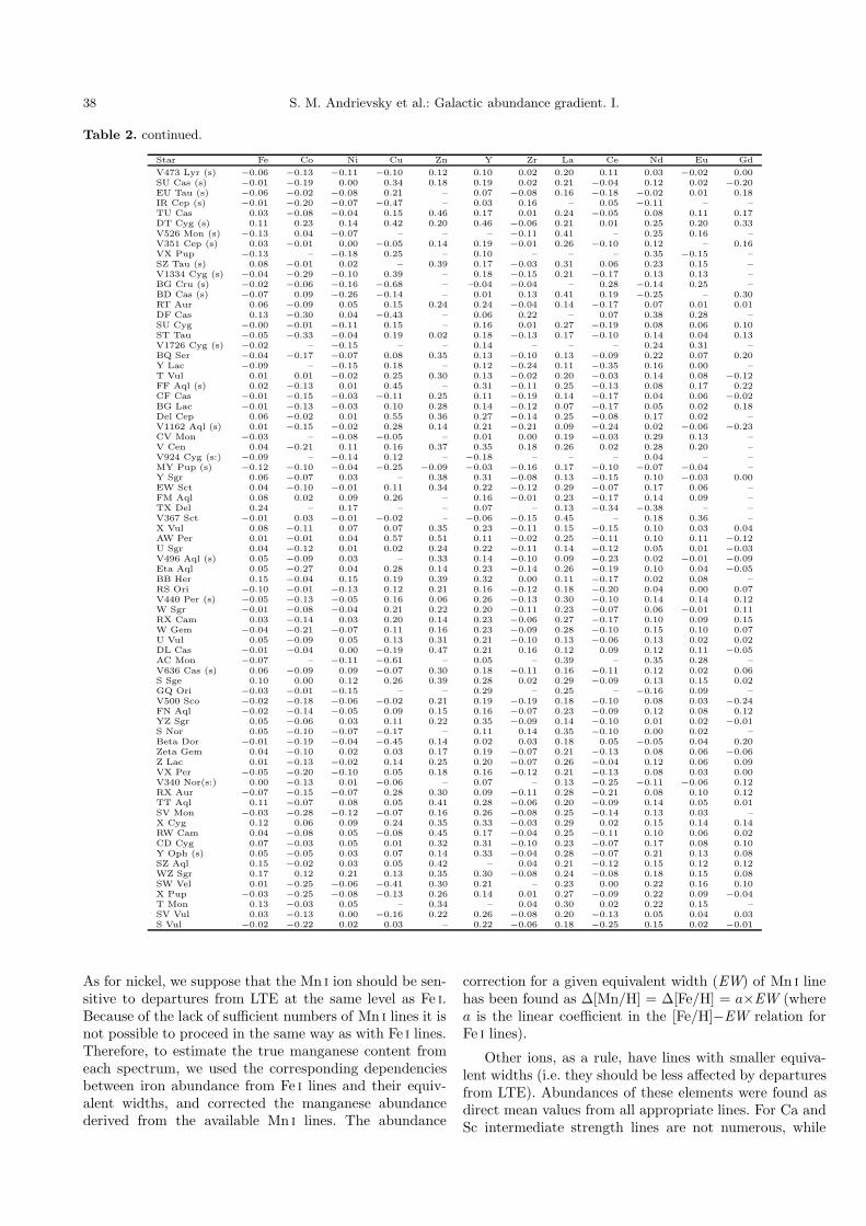
Table 2. continued.

Star Fe Co Ni Cu Zn Y Zr La Ce Nd Eu Gd

V473 Lyr (s) −0.06 −0.13 −0.11 −0.10 0.12 0.10 0.02 0.20 0.11 0.03 −0.02 0.00SU Cas (s) −0.01 −0.19 0.00 0.34 0.18 0.19 0.02 0.21 −0.04 0.12 0.02 −0.20EU Tau (s) −0.06 −0.02 −0.08 0.21 – 0.07 −0.08 0.16 −0.18 −0.02 0.01 0.18IR Cep (s) −0.01 −0.20 −0.07 −0.47 – 0.03 0.16 – 0.05 −0.11 – –TU Cas 0.03 −0.08 −0.04 0.15 0.46 0.17 0.01 0.24 −0.05 0.08 0.11 0.17DT Cyg (s) 0.11 0.23 0.14 0.42 0.20 0.46 −0.06 0.21 0.01 0.25 0.20 0.33V526 Mon (s) −0.13 0.04 −0.07 – – – −0.11 0.41 – 0.25 0.16 –V351 Cep (s) 0.03 −0.01 0.00 −0.05 0.14 0.19 −0.01 0.26 −0.10 0.12 – 0.16VX Pup −0.13 – −0.18 0.25 – 0.10 – – – 0.35 −0.15 –SZ Tau (s) 0.08 −0.01 0.02 – 0.39 0.17 −0.03 0.31 0.06 0.23 0.15 –V1334 Cyg (s) −0.04 −0.29 −0.10 0.39 – 0.18 −0.15 0.21 −0.17 0.13 0.13 –BG Cru (s) −0.02 −0.06 −0.16 −0.68 – –0.04 −0.04 – 0.28 −0.14 0.25 –BD Cas (s) −0.07 0.09 −0.26 −0.14 – 0.01 0.13 0.41 0.19 −0.25 – 0.30RT Aur 0.06 −0.09 0.05 0.15 0.24 0.24 −0.04 0.14 −0.17 0.07 0.01 0.01DF Cas 0.13 −0.30 0.04 −0.43 – 0.06 0.22 – 0.07 0.38 0.28 –SU Cyg −0.00 −0.01 −0.11 0.15 – 0.16 0.01 0.27 −0.19 0.08 0.06 0.10ST Tau −0.05 −0.33 −0.04 0.19 0.02 0.18 −0.13 0.17 −0.10 0.14 0.04 0.13V1726 Cyg (s) −0.02 – −0.15 – – 0.14 – – – 0.24 0.31 –BQ Ser −0.04 −0.17 −0.07 0.08 0.35 0.13 −0.10 0.13 −0.09 0.22 0.07 0.20Y Lac −0.09 – −0.15 0.18 – 0.12 −0.24 0.11 −0.35 0.16 0.00 –T Vul 0.01 0.01 −0.02 0.25 0.30 0.13 −0.02 0.20 −0.03 0.14 0.08 −0.12FF Aql (s) 0.02 −0.13 0.01 0.45 – 0.31 −0.11 0.25 −0.13 0.08 0.17 0.22CF Cas −0.01 −0.15 −0.03 −0.11 0.25 0.11 −0.19 0.14 −0.17 0.04 0.06 −0.02BG Lac −0.01 −0.13 −0.03 0.10 0.28 0.14 −0.12 0.07 −0.17 0.05 0.02 0.18Del Cep 0.06 −0.02 0.01 0.55 0.36 0.27 −0.14 0.25 −0.08 0.17 0.02 –V1162 Aql (s) 0.01 −0.15 −0.02 0.28 0.14 0.21 −0.21 0.09 −0.24 0.02 −0.06 −0.23CV Mon −0.03 – −0.08 −0.05 – 0.01 0.00 0.19 −0.03 0.29 0.13 –V Cen 0.04 −0.21 0.11 0.16 0.37 0.35 0.18 0.26 0.02 0.28 0.20 –V924 Cyg (s:) −0.09 – −0.14 0.12 – −0.18 – – – 0.04 – –MY Pup (s) −0.12 −0.10 −0.04 −0.25 −0.09 −0.03 −0.16 0.17 −0.10 −0.07 −0.04 –Y Sgr 0.06 −0.07 0.03 – 0.38 0.31 −0.08 0.13 −0.15 0.10 −0.03 0.00EW Sct 0.04 −0.10 −0.01 0.11 0.34 0.22 −0.12 0.29 −0.07 0.17 0.06 –FM Aql 0.08 0.02 0.09 0.26 – 0.16 −0.01 0.23 −0.17 0.14 0.09 –TX Del 0.24 – 0.17 – – 0.07 – 0.13 −0.34 −0.38 – –V367 Sct −0.01 0.03 −0.01 −0.02 – −0.06 −0.15 0.45 – 0.18 0.36 –X Vul 0.08 −0.11 0.07 0.07 0.35 0.23 −0.11 0.15 −0.15 0.10 0.03 0.04AW Per 0.01 −0.01 0.04 0.57 0.51 0.11 −0.02 0.25 −0.11 0.10 0.11 −0.12U Sgr 0.04 −0.12 0.01 0.02 0.24 0.22 −0.11 0.14 −0.12 0.05 0.01 −0.03V496 Aql (s) 0.05 −0.09 0.03 – 0.33 0.14 −0.10 0.09 −0.23 0.02 −0.01 −0.09Eta Aql 0.05 −0.27 0.04 0.28 0.14 0.23 −0.14 0.26 −0.19 0.10 0.04 −0.05BB Her 0.15 −0.04 0.15 0.19 0.39 0.32 0.00 0.11 −0.17 0.02 0.08 –RS Ori −0.10 −0.01 −0.13 0.12 0.21 0.16 −0.12 0.18 −0.20 0.04 0.00 0.07V440 Per (s) −0.05 −0.13 −0.05 0.16 0.06 0.26 −0.13 0.30 −0.10 0.14 0.14 0.12W Sgr −0.01 −0.08 −0.04 0.21 0.22 0.20 −0.11 0.23 −0.07 0.06 −0.01 0.11RX Cam 0.03 −0.14 0.03 0.20 0.14 0.23 −0.06 0.27 −0.17 0.10 0.09 0.15W Gem −0.04 −0.21 −0.07 0.11 0.16 0.23 −0.09 0.28 −0.10 0.15 0.10 0.07U Vul 0.05 −0.09 0.05 0.13 0.31 0.21 −0.10 0.13 −0.06 0.13 0.02 0.02DL Cas −0.01 −0.04 0.00 −0.19 0.47 0.21 0.16 0.12 0.09 0.12 0.11 −0.05AC Mon −0.07 – −0.11 −0.61 – 0.05 – 0.39 – 0.35 0.28 –V636 Cas (s) 0.06 −0.09 0.09 −0.07 0.30 0.18 −0.11 0.16 −0.11 0.12 0.02 0.06S Sge 0.10 0.00 0.12 0.26 0.39 0.28 0.02 0.29 −0.09 0.13 0.15 0.02GQ Ori −0.03 −0.01 −0.15 – – 0.29 – 0.25 – −0.16 0.09 –V500 Sco −0.02 −0.18 −0.06 −0.02 0.21 0.19 −0.19 0.18 −0.10 0.08 0.03 −0.24FN Aql −0.02 −0.14 −0.05 0.09 0.15 0.16 −0.07 0.23 −0.09 0.12 0.08 0.12YZ Sgr 0.05 −0.06 0.03 0.11 0.22 0.35 −0.09 0.14 −0.10 0.01 0.02 −0.01S Nor 0.05 −0.10 −0.07 −0.17 – 0.11 0.14 0.35 −0.10 0.00 0.02 –Beta Dor −0.01 −0.19 −0.04 −0.45 0.14 0.02 0.03 0.18 0.05 −0.05 0.04 0.20Zeta Gem 0.04 −0.10 0.02 0.03 0.17 0.19 −0.07 0.21 −0.13 0.08 0.06 −0.06Z Lac 0.01 −0.13 −0.02 0.14 0.25 0.20 −0.07 0.26 −0.04 0.12 0.06 0.09VX Per −0.05 −0.20 −0.10 0.05 0.18 0.16 −0.12 0.21 −0.13 0.08 0.03 0.00V340 Nor(s:) 0.00 −0.13 0.01 −0.06 – 0.07 – 0.13 −0.25 −0.11 −0.06 0.12RX Aur −0.07 −0.15 −0.07 0.28 0.30 0.09 −0.11 0.28 −0.21 0.08 0.10 0.12TT Aql 0.11 −0.07 0.08 0.05 0.41 0.28 −0.06 0.20 −0.09 0.14 0.05 0.01SV Mon −0.03 −0.28 −0.12 −0.07 0.16 0.26 −0.08 0.25 −0.14 0.13 0.03 –X Cyg 0.12 0.06 0.09 0.24 0.35 0.33 −0.03 0.29 0.02 0.15 0.14 0.14RW Cam 0.04 −0.08 0.05 −0.08 0.45 0.17 −0.04 0.25 −0.11 0.10 0.06 0.02CD Cyg 0.07 −0.03 0.05 0.01 0.32 0.31 −0.10 0.23 −0.07 0.17 0.08 0.10Y Oph (s) 0.05 −0.05 0.03 0.07 0.14 0.33 −0.04 0.28 −0.07 0.21 0.13 0.08SZ Aql 0.15 −0.02 0.03 0.05 0.42 – 0.04 0.21 −0.12 0.15 0.12 0.12WZ Sgr 0.17 0.12 0.21 0.13 0.35 0.30 −0.08 0.24 −0.08 0.18 0.15 0.08SW Vel 0.01 −0.25 −0.06 −0.41 0.30 0.21 – 0.23 0.00 0.22 0.16 0.10X Pup −0.03 −0.25 −0.08 −0.13 0.26 0.14 0.01 0.27 −0.09 0.22 0.09 −0.04T Mon 0.13 −0.03 0.05 – 0.34 – 0.04 0.30 0.02 0.22 0.15 –SV Vul 0.03 −0.13 0.00 −0.16 0.22 0.26 −0.08 0.20 −0.13 0.05 0.04 0.03S Vul −0.02 −0.22 0.02 0.03 – 0.22 −0.06 0.18 −0.25 0.15 0.02 −0.01

As for nickel, we suppose that the Mn i ion should be sen-sitive to departures from LTE at the same level as Fe i.Because of the lack of sufficient numbers of Mn i lines it isnot possible to proceed in the same way as with Fe i lines.Therefore, to estimate the true manganese content fromeach spectrum, we used the corresponding dependenciesbetween iron abundance from Fe i lines and their equiv-alent widths, and corrected the manganese abundancederived from the available Mn i lines. The abundance

correction for a given equivalent width (EW) of Mn i linehas been found as ∆[Mn/H] = ∆[Fe/H] = a×EW (wherea is the linear coefficient in the [Fe/H]−EW relation forFe i lines).

Other ions, as a rule, have lines with smaller equiva-lent widths (i.e. they should be less affected by departuresfrom LTE). Abundances of these elements were found asdirect mean values from all appropriate lines. For Ca andSc intermediate strength lines are not numerous, while


0

1000

2000

3000

4000

5000

0

30

60

90

120

150

180

210

240

270

300

330

0

1000

2000

3000

4000

5000

d, pc

Fig. 4. The distribution of the program Cepheids in the galactic plane.

weak lines are often absent. For these two elements abun-dance corrections were not determined. Therefore, theirabundances should be interpreted with caution.

5. Distances

Galactocentric distances for the program Cepheids werecalculated from the following formula (the distances aregiven in pc):

RG =[R2

G, + (d cos b)2 − 2RG,d cos b cos l]1/2

(1)

where RG, is the galactocentric distance of the Sun, d isthe heliocentric distance of the Cepheid, l is the galacticlongitude, and b is the galactic latitude. The heliocentricdistance d is given by

d = 10−0.2(Mv−<V>−5+Av). (2)

To estimate the heliocentric distances of programCepheids we used the “absolute magnitude – pulsationalperiod” relation of Gieren et al. (1998). E(B − V ),< B − V >, mean visual magnitudes and pulsational pe-riods are from Fernie et al. (1995), see Table 3. We use forAv an expression from Laney & Stobie (1993):

Av = [3.07 + 0.28(B − V )0 + 0.04E(B − V )]E(B−V )·(3)

For s-Cepheids (DCEPS type) the observed periods arethose of the first overtone (see, e.g. Christensen-Dalsgaard& Petersen 1995). Therefore, for these stars the corre-sponding periods of the unexcited fundamental mode werefound using the ratio P1/P0 ≈ 0.72, and these periodswere then used to estimate the absolute magnitudes. In thecase of V473 Lyr, the fundamental period P0 was foundassuming that this star pulsates in the second overtone(Andrievsky et al. 1998), i.e. P1/P0 = 0.56. For V924 Cyg

and V340 Nor, whose association with the group of s-Cepheids is not certain, we used the observed periods asthe fundamental period in order to estimate Mv.

The galactocentric distance of the Sun RG, = 7.9 kpcwas adopted from the recent determination by McNamaraet al. (2000). Estimated distances and other useful charac-teristics of our program Cepheids are gathered in Table 3.Because our spectra were obtained with different spectro-graphs having differing resolving powers, and also becausefor different stars we have a differing number of spectra(as a rule, one spectrum for Cepheids observed with 6-mtelescope), we have assigned for each star a weight in thederivation of the gradient solution. We assigned a weightW = 1 to the following stars: those observed with the6-m telescope (lower resolution spectra), the two starsobserved by Harris & Pilachowski (1984), and the starswith one high resolution spectrum, but a low S/N ratio(VX Pup, CV Mon and MY Pup). For the rest of the pro-gram stars a weight W = 3 was used. The weights aregiven in the last column of Table 3. The distribution ofthe analyzed Cepheids in the galactic plane is shown inFig. 4.

6. Results and discussion

6.1. The radial distribution of elemental abundances:General picture and remarks on some elements

Using our calculated galactocentric distances and averageabundances we can determine the galactic metallicity gra-dient from a number of species. Plots for several chemicalelements and results of a linear fit are given in Fig. 5 (iron)and Figs. 6–9 (other elements). Note that, in the plotsfor Si and Cr, TX Del is not included. This star showsrather strong excess in the abundances of these elements


Table 3. Some physical and positional characteristics of program Cepheids.

Star P , d < B − V > E(B − V ) Mv d, pc l b RG, kpc <[Fe/H]> W

V473 Lyr (s) 2.6600 0.632 0.026 −2.47 517.2 60.56 7.44 7.66 −0.06 3SU Cas (s) 2.7070 0.703 0.287 −2.49 322.7 133.47 8.52 8.12 −0.01 3EU Tau (s) 2.9200 0.664 0.172 −2.58 1058.2 188.80 −5.32 8.94 −0.06 3IR Cep (s) 2.9360 0.870 0.411 −2.59 624.4 103.40 4.91 8.07 −0.01 1

TU Cas 2.1393 0.582 0.115 −2.21 821.4 118.93 −11.40 8.32 +0.03 3DT Cyg (s) 3.4720 0.538 0.039 −2.79 487.4 76.55 −10.78 7.80 +0.11 3

V526 Mon (s) 3.7150 0.593 0.093 −2.87 1716.6 215.13 1.81 9.36 −0.13 1V351 Cep (s) 3.8970 0.940 0.400 −2.93 1640.5 105.20 −0.72 8.48 +0.03 1

VX Pup 3.0109 0.610 0.136 −2.62 1265.5 237.02 −1.30 8.65 −0.13 1SZ Tau (s) 4.3730 0.844 0.294 −3.07 536.5 179.48 −18.74 8.41 +0.08 3

V1334 Cyg(s) 4.6290 0.504 0.000 −3.14 633.2 83.60 −7.95 7.85 −0.04 3BG Cru (s) 4.6430 0.606 0.053 −3.14 491.2 300.42 3.35 7.66 −0.02 3BD Cas (s) 3.6510 – 0.734 −3.25 2371.5 118.00 −0.96 9.25 −0.07 1

RT Aur 3.7282 0.595 0.051 −2.88 428.2 183.15 8.92 8.32 +0.06 3DF Cas 3.8328 1.181 0.599 −2.91 2297.9 136.00 1.53 9.68 +0.13 1SU Cyg 3.8455 0.575 0.096 −2.91 781.5 64.76 2.50 7.60 −0.00 3ST Tau 4.0343 0.847 0.355 −2.97 1020.7 193.12 −8.05 8.89 −0.05 3

V1726 Cyg(s) 5.8830 0.885 0.312 −3.43 1916.2 92.50 −1.61 8.21 −0.02 1BQ Ser 4.2709 1.399 0.841 −3.04 911.7 35.13 5.37 7.18 −0.04 3Y Lac 4.3238 0.731 0.217 −3.05 1996.6 98.72 −4.03 8.43 −0.09 3T Vul 4.4355 0.635 0.064 −3.09 532.7 72.13 −10.15 7.76 +0.01 3

FF Aql (s) 6.2100 0.756 0.224 −3.49 424.4 49.20 6.36 7.63 +0.02 3CF Cas 4.8752 1.174 0.566 −3.20 3145.2 116.58 −0.99 9.72 −0.01 3TV Cam 5.2950 1.198 0.644 −3.30 3739.1 145.02 6.15 11.15 −0.06 1BG Lac 5.3319 0.949 0.336 −3.31 1656.6 92.97 −9.26 8.15 −0.01 3Del Cep 5.3663 0.657 0.092 −3.31 247.9 105.19 0.53 7.97 +0.06 3

V1162 Aql(s) 7.4670 0.900 0.205 −3.71 1470.2 29.40 −18.60 6.72 +0.01 3CV Mon 5.3789 1.297 0.714 −3.32 1809.1 208.57 −1.79 9.53 −0.03 1V Cen 5.4939 0.875 0.289 −3.34 702.3 316.40 3.31 7.41 +0.04 3

V924 Cyg 5.5710 0.847 0.258 −3.36 4428.4 66.90 5.33 7.38 −0.09 1MY Pup (s) 7.9100 0.631 0.064 −3.78 708.4 261.31 −12.86 8.03 −0.12 1

Y Sgr 5.7734 0.856 0.205 −3.40 496.1 12.79 −2.13 7.42 +0.06 3EW Sct 5.8233 1.725 1.128 −3.41 345.0 25.34 −0.09 7.59 +0.04 3FM Aql 6.1142 1.277 0.646 −3.47 842.3 44.34 0.89 7.32 +0.08 3TX Del 6.1660 0.766 0.132 −3.48 2782.5 50.96 −24.26 6.60 +0.24 3

V367 Sct 6.2931 1.769 1.130 −3.51 1887.7 21.63 −0.83 6.18 −0.01 3X Vul 6.3195 1.389 0.848 −3.51 831.6 63.86 −1.28 7.57 +0.08 3

AW Per 6.4636 1.055 0.534 −3.54 724.9 166.62 −5.39 8.60 +0.01 3U Sgr 6.7452 1.087 0.403 −3.59 620.5 13.71 −4.46 7.30 +0.04 3

V496 Aql (s) 9.4540 1.146 0.413 −4.00 1195.1 28.20 −7.13 6.88 +0.05 3Eta Aql 7.1767 0.789 0.149 −3.66 260.1 40.94 −13.07 7.71 +0.05 3BB Her 7.5080 1.100 0.414 −3.72 3091.7 43.30 6.81 6.04 +0.15 3RS Ori 7.5669 0.945 0.389 −3.73 1498.9 196.58 0.35 9.35 −0.10 3

V440 Per (s) 10.5140 0.873 0.273 −4.12 801.1 135.87 −5.17 8.49 −0.05 3W Sgr 7.5949 0.746 0.111 −3.73 405.4 1.58 −3.98 7.50 −0.01 3

RX Cam 7.9120 1.193 0.569 −3.78 833.4 145.90 4.70 8.60 +0.03 3W Gem 7.9138 0.889 0.283 −3.78 916.9 197.43 3.38 8.78 −0.04 3U Vul 7.9906 1.275 0.654 −3.79 570.9 56.07 −0.29 7.60 +0.05 3

DL Cas 8.0007 1.154 0.533 −3.79 1602.1 120.27 −2.55 8.82 −0.01 3AC Mon 8.0143 1.165 0.508 −3.80 2754.8 221.80 −1.86 10.12 −0.07 1

V636 Cas (s) 11.6350 1.391 0.786 −4.25 592.2 127.50 1.09 8.27 +0.06 3S Sge 8.3821 0.805 0.127 −3.85 648.1 55.17 −6.12 7.55 +0.10 3

GQ Ori 8.6161 0.976 0.279 −3.88 2437.6 199.77 −4.42 10.22 −0.03 1V500 Sco 9.3168 1.276 0.599 −3.98 1406.1 359.02 −1.35 6.49 −0.02 3FN Aql 9.4816 1.214 0.510 −4.00 1383.2 38.54 −3.11 6.87 −0.02 3YZ Sgr 9.5536 1.032 0.292 −4.01 1205.4 17.75 −7.12 6.77 +0.05 3S Nor 9.7542 0.941 0.215 −4.03 879.6 327.80 −5.39 7.17 +0.05 3

Beta Dor 9.8424 0.807 0.044 −4.04 335.8 271.73 −32.78 7.90 −0.01 3Zeta Gem 10.1507 0.798 0.018 −4.08 387.2 195.75 11.90 8.27 +0.04 3

Z Lac 10.8856 1.095 0.404 −4.17 1782.4 105.76 −1.62 8.56 +0.01 3VX Per 10.8890 1.158 0.515 −4.17 2283.5 132.80 −2.96 9.60 −0.05 3

V340 Nor(s:) 11.2870 1.149 0.332 −4.21 1976.1 329.80 −2.23 6.27 +0.00 3RX Aur 11.6235 1.009 0.276 −4.24 1579.0 165.77 −1.28 9.44 −0.07 3TT Aql 13.7547 1.292 0.495 −4.45 976.1 36.00 −3.14 7.13 +0.11 3SV Mon 15.2328 1.048 0.249 −4.57 2472.3 203.74 −3.67 10.21 −0.03 3X Cyg 16.3863 1.130 0.288 −4.66 1043.5 76.87 −4.26 7.73 +0.12 3

RW Cam 16.4148 1.351 0.649 −4.66 1748.4 144.85 3.80 9.38 +0.04 3CD Cyg 17.0740 1.266 0.514 −4.71 2462.1 71.07 1.43 7.47 +0.07 3

Y Oph (s) 23.7880 1.377 0.655 −5.11 664.9 20.60 10.12 7.29 +0.05 3SZ Aql 17.1408 1.389 0.641 −4.71 1731.0 35.60 −2.34 6.57 +0.15 3YZ Aur 18.1932 1.375 0.565 −4.78 4444.7 167.28 0.94 12.27 −0.05 1WZ Sgr 21.8498 1.392 0.467 −5.00 1967.5 12.11 −1.32 5.99 +0.17 3SW Vel 23.4410 1.162 0.349 −5.09 2572.4 266.20 −3.00 8.47 +0.01 3X Pup 25.9610 1.127 0.443 −5.21 2776.6 236.14 −0.78 9.72 −0.03 3T Mon 27.0246 1.166 0.209 −5.26 1369.7 203.63 −2.55 9.17 +0.13 3SV Vul 44.9948 1.442 0.570 −5.87 1729.5 63.95 0.32 7.31 +0.03 3S Vul 68.4640 1.892 0.827 −6.38 3199.7 63.45 0.83 7.07 −0.02 3

which could be connected with its peculiar nature (inHarris & Welch 1989 TX Del is reported as a spectro-scopic binary. It has also been labeled a Type II Cepheid attimes). In the plot for carbon we did not include the datafor FN Aql and SV Mon, both of which have an extremelylow carbon abundances. These two unusual Cepheids willbe discussed in detail in a separate paper.

The information in the plots and also in Fig. 10 enablesone to put together several important conclusions. Mostradial distributions of the elements studied indicate a neg-ative gradient ranging from about −0.02 dex kpc−1 to−0.06 dex kpc−1, with an average of −0.03 dex kpc−1 forthe elements in Figs. 5–8. The most reliable value comesfrom iron (typically the number of iron lines for each star isabout 200–300). The gradient in iron is −0.029 dex kpc−1,


5 6 7 8 9 10 11 12 13-0.50

-0.25

0.00

0.25

0.50

r = -0.471

[Fe/H]= -0.029*RG + 0.253

±0.004 ±0.031

[Fe/

H]

RG, kpc

Fig. 5. Iron abundance gradient and its linear approximation. The position of the Sun is at the intersection of the dashed lines.

which is close to the typical gradient value produced byother iron-group elements. Examination of Fig. 5 mightlead one to suspect that the iron gradient is being con-trolled by the cluster of stars atR ≈ 6.5 with [Fe/H]≈ 0.2.If one deletes these stars from the solution the gradi-ent falls to approximately −0.02 dex kpc−1. This lattervalue differs from the value determined using all the databy about twice the formal uncertainty in either slope.However, we do not favour the neglect these points asthere is no reason to suspect these abundances relative tothe bulk of the objects. Indeed, in a subsequent paper, weshall present results for Cepheids which lie closer to thegalactic center and which have abundances above those ofthis study, which may imply a steepening of the gradienttowards the galactic center.

Unweighted iron abundances give a gradient of−0.028 dex kpc−1. Both weighted and unweighted irongradients are not significantly changed if we remove twoCepheids at galactocentric distances greater than 11 kpc(gradient is −0.031 dex kpc−1). Thus, the average slopeof about −0.03 dex kpc−1 probably applies to the range6 ≤ RG (kpc) ≤ 10. Notice that in all cases the correlationcoefficient is relatively low, r ≈ 0.47.

Carbon shows a surprisingly clear dependence upongalactocentric distance (Fig. 6a): the slope of the rela-tion is among the largest from examined elements. Wehave included in the present study elements such as car-bon and sodium, although the gradients based on theirabundances determined from Cepheids may not be con-clusive. In fact, it is quite likely that the surface abun-dances of these elements have been altered in these inter-mediate mass stars during their evolution from the mainsequence to the Cepheid stage. For example, the surfaceabundance of carbon should be decreased after the globalmixing which brings the CNO-processed material into thestellar atmosphere (turbulent diffusion in the progenitor Bmain sequence star, or the first dredge-up in the red giantphase). Some decrease in the surface abundance of oxygenis also expected for supergiant stars, but at a significantlylower level than for carbon (Schaller et al. 1992).

It is also well known that galactic supergiants(Cepheids, in particular) show an increased sodium abun-dance which is usually interpreted as a result of dredge-upof material processed in the Ne–Na cycle (and thereforeenriched in sodium) to the stellar surface (Sasselov 1986;Luck 1994; Denissenkov 1993a, 1993b, 1994). Such a con-tamination of the Cepheids’ atmospheres with additionalsodium may result in a bias of the [Na/H] gradient valuederived from Cepheids in relation to the true gradient. Itcan be seen that our results in Figs. 6a,c are consistentwith these considerations on C and Na, respectively. It isnot clear how these effects should affect stars at differentgalactocentric distances (with different metallicities), butit is likely that they contribute to increase the dispersionin the abundances, thus producing a flatter gradient.

There are some indications (Andrievsky & Kovtyukh1996) that surface Mg and Al abundances in yellow super-giants can be altered to some extent due to mixing of thematerial processed in the Mg–Al cycle with atmosphericgas. This supposition seems to gain some additional sup-port from our present data (see Fig. 11) where one can seethat the Mg and Al abundances are correlated.

As surface abundance modifications depend upon thenumber of visits to the red giant region (i.e. the number ofdredge-up events) as well as other factors (pre dredge-upevents, depth of mixing events, mass), it is possible thatthe program Cepheids could show differential evolution-ary effects in their abundances. Because of the high prob-ability of such effects impacting the observed carbon andsodium (and perhaps, oxygen, magnesium, and aluminum)abundances in these Cepheids, we recommend that ourgradient values for carbon and sodium to be viewed withextreme caution, while the gradients of oxygen, magne-sium and aluminum abundances could be used, but alsowith some caution.

The difference in metallicity between the stars of oursample (say, at 6 kpc and 10 kpc) is about 0.25 dex.This is a rather small value to detect/investigate the so-called “odd-even” effect, that is the metallicity dependentyield for some elements which should be imprinted on


5 6 7 8 9 10 11-1.0

-0.5

0.0

0.5

1.0

f

[Si/H]= -0.030*RG + 0.299

±0.004 ±0.034

[Si/H

]

-1.0

-0.5

0.0

0.5

1.0

b[O/H]= -0.022*RG + 0.102

±0.009 ±0.074

[O/H

]

-1.0

-0.5

0.0

0.5

1.0

e

[Al/H]= -0.041*RG + 0.444

±0.005 ±0.043

[Al/H

]

-1.0

-0.5

0.0

0.5

1.0

c

[Na/H]= -0.023*RG + 0.380

±0.006 ±0.052

[Na/

H]

-1.0

-0.5

0.0

0.5

1.0

a[C/H]= -0.055*RG + 0.230

±0.006 ±0.050

[C/H

]

-1.0

-0.5

0.0

0.5

1.0

RG , kpc

d[Mg/H]= -0.015*RG - 0.067

±0.009 ±0.071

[Mg/

H]

Fig. 6. Abundance gradients for other investigated elements: C–Si.

the trends of abundance ratios for [Elodd/Eleven] versusgalactocentric distance, see for details Hou et al. (2000).Such elements as, for example, aluminum, scandium, vana-dium and manganese should show progressively decreasingabundances with overall metal decrease. This should man-ifest itself as a gradient in [Elodd/Fe]. We have plotted theabundance ratios for some “odd” elements (normalizedto iron abundance) versus RG in Fig. 12. As one can see,

none of the abundance ratios plotted versus galactocentricdistance shows a clear dependence upon RG. This couldmean that the “odd-even” effect may be overestimated ifonly the yields from massive stars are taken into accountignoring other possible sources, or that the effect is notsufficiently large to be seen over the current distance andmetallicity baseline.


5 6 7 8 9 10 11-1.0

-0.5

0.0

0.5

1.0

f

[Cr/H]= -0.019*RG + 0.205

±0.007 ±0.059

[Cr/

H]

-1.0

-0.5

0.0

0.5

1.0

b

[Ca/H]= -0.021*RG + 0.140

±0.006 ±0.049

[Ca/

H]

-1.0

-0.5

0.0

0.5

1.0

e

[V/H]= -0.035*RG + 0.296

±0.006 ±0.045

[V/H

]

-1.0

-0.5

0.0

0.5

1.0

c[Sc/H]= -0.032*RG + 0.192

±0.011 ±0.088

[Sc/

H]

-1.0

-0.5

0.0

0.5

1.0

a

[S/H]= -0.051*RG + 0.530

±0.008 ±0.061[S/H

]

-1.0

-0.5

0.0

0.5

1.0

RG , kpc

d

[Ti/H]= -0.017*RG + 0.186

±0.005 ±0.039

[Ti/H

]

Fig. 7. Same as Fig. 6, but for S–Cr.

6.2. Metallicity dispersion and the metallicity in thesolar vicinity

There is a spread in the metallicity at each given galac-tocentric distance (larger than the standard error of theabundance analysis) which is most likely connected withlocal inhomogeneities in the galactic disc. As an example,in Fig. 13, we show the derived iron abundance vs. galactic

longitude for the stars of our sample (a few Cepheids withheliocentric distances large than 3000 pc were excluded).The distribution gives only a small hint about a local in-crease of the metallicity in the solar vicinity towards thedirection l ≈ 30 and 150.

It is important to note that at the solar galactocentricdistance those elements, whose abundance is not supposed


5 6 7 8 9 10 11-1.0

-0.5

0.0

0.5

1.0

f

[Y/H]= -0.022*RG + 0.365

±0.007 ±0.058

[Y/H

]

-1.0

-0.5

0.0

0.5

1.0

b[Co/H]= -0.024*RG + 0.094

±0.007 ±0.059

[Co/

H]

-1.0

-0.5

0.0

0.5

1.0

e

[Zn/H]= -0.015*RG + 0.389

±0.010 ±0.077

[Zn/

H]

-1.0

-0.5

0.0

0.5

1.0

c

[Ni/H]= -0.037*RG + 0.283

±0.005 ±0.042

[Ni/H

]

-1.0

-0.5

0.0

0.5

1.0

a

[Mn/H]= -0.034*RG + 0.294

±0.007 ±0.058[Mn/

H]

-1.0

-0.5

0.0

0.5

1.0

RG , kpc

d

[Cu/H]= -0.028*RG + 0.304

±0.018 ±0.141

[Cu/

H]

Fig. 8. Same as Fig. 6, but for Mn–Y.

to be changed in supergiants during their evolution, showon average the solar abundance in Cepheids. Relative tothe solar region, the stars within our sample which arewithin 500 pc of the Sun have a mean [Fe/H] of ≈+ 0.01(n = 14, σ = 0.06). If we consider all program stars at agalactocentric radius of 7.4–8.4 kpc, i.e. those in a 1 kpcwide annulus centered at the solar radius, we find a mean[Fe/H] of approximately +0.03 (n = 29, σ = 0.05).

This result again stresses the importance of the prob-lem connected with subsolar metallicities reported forthe hot stars from the solar vicinity (see, e.g. Gies &Lambert 1992; Cunha & Lambert 1994; Kilian 1992;Kilian et al. 1994; Daflon et al. 1999; Andrievsky et al.1999). This also follows from the plots provided byGummersbach et al. (1998) for several elements.


5 6 7 8 9 10 11-1.0

-0.5

0.0

0.5

1.0

f[Gd/H]= +0.014*RG - 0.063

±0.010 ±0.082

[Gd/

H]

-1.0

-0.5

0.0

0.5

1.0

b

[La/H]= +0.018*RG + 0.072

±0.005 ±0.040

[La/

H]

-1.0

-0.5

0.0

0.5

1.0

e

[Eu/H]= +0.007*RG + 0.012

±0.006 ±0.044

[Eu/

H]

-1.0

-0.5

0.0

0.5

1.0

c[Ce/H]= +0.011*RG - 0.183

±0.008 ±0.062

[Ce/

H]

-1.0

-0.5

0.0

0.5

1.0

a[Zr/H]= + 0.002*RG - 0.075

±0.007 ±0.053

[Zr/

H]

-1.0

-0.5

0.0

0.5

1.0

RG , kpc

d[Nd/H]= +0.017*RG - 0.033

±0.007 ±0.058

[Nd/

H]

Fig. 9. Same as Fig. 6, but for Zr–Gd.

This problem was discussed, for instance, by Luck et al.(2000). The authors compared the elemental abundancesof B stars from the open cluster M 25 with those of theCepheid U Sgr and two cool supergiants which are alsomembers of the cluster, and found disagreement in theabundances of the B stars and supergiants; e.g., whilethe supergiants of M 25 show nearly solar abundances,

the sample of B stars demonstrate a variety of patternsfrom under- to over-abundances. This should not be ob-served if we assume that all stars in the cluster were bornfrom the same parental nebula. Obviously, the problem ofsome disagreement between abundance results from youngsupergiants and main-sequence stars requires furtherinvestigation.


5 15 25 35 45 55 65-0.10

-0.05

0.00

0.05

0.10

Na Al Sc V Mn Co Cu Y La Eu

C O Mg Si S Ca Ti Cr Fe Ni Zn Zr Ce Nd Gd

Gra

dien

t

Z

Fig. 10. Derived gradients versus atomic number.

-0.5 -0.4 -0.3 -0.2 -0.1 0.0 0.1 0.2-0.2

-0.1

0.0

0.1

0.2

0.3

0.4

0.5

[Al/H]= 0.394*[Mg/H] + 0.194 ±0.052 ±0.011

[Al/H

]

[Mg/H]

Fig. 11. [Al/H] vs. [Mg/H] for program Cepheids.

6.3. Flattening of the elemental distribution in thesolar neighbourhood

All previous studies of the radial abundance distribu-tion in the galactic disc have considered only chemicalelements from carbon to iron, and all derived gradientshave shown a progressive decrease in abundance with in-creasing galactocentric distance. For the elements fromcarbon to yttrium in this study our gradient values alsohave negative signs, while for the heavier species (fromzirconium to gadolinium) we obtained (within the errorbars) near-to-zero gradients (see Fig. 10). Two obviousfeatures which are inherent to derived C-Gd abundancedistributions have to be interpreted: a rather flat charac-ter of the distribution for light/iron-group elements, andan apparent absence of a clear gradient for heavy species.

The flattening of the abundance distribution can becaused by radial flows in the disc which may lead to a ho-mogenization of ISM. Among the possible sources forcinggas of ISM to flow in the radial direction, and thereforeproducing a net mixing effect there could be a gas vis-cosity in the disc, gas infall from the halo, gravitational

interaction between gas and spiral waves or a central bar(see e.g., Lacey & Fall 1985; Portinari & Chiosi 2000).

The mechanism of the angular momentum re-distribution in the disc based on the gas infall from thehalo is dependent upon the infall rate, and therefore itshould have been important at the earlier stages of theGalaxy evolution, while other sources of the radial flowsshould effectively operate at present.

Gravitational interaction between the gas and densitywaves produces the radial flows with velocity (Lacey &Fall 1985):

vr ∼ (Ωp − Ωc)−1, (4)

where Ωp and Ωc are the angular velocities of the spi-ral wave and the disc rotation respectively. According toAmaral & Lepine (1997) and Mishurov et al. (1997) amongothers, based on several different arguments, the galacticco-rotation resonance is located close to the solar galac-tic orbit. The co-rotation radius is the radius at whichthe galactic rotation velocity coincides with the rotationvelocity of the spiral pattern. Together with Eq. (4) thismeans that, inside the co-rotation circle, gas flows towardsthe galactic center (Ωc > Ωp and vr < 0), while out-side it flows outwards. This mechanism can produce some“cleaning” effect in the solar vicinity, and thus can leadto some flattening of the abundance distribution. In addi-tion, it could explain the similarity in the solar abundancesand mean abundances in the five billion years youngerCepheids located at the solar galactocentric annulus (seeFig. 5), although one might expect that the Cepheids fromthis region should be more abundant in metals than ourSun.

There is a clear evidence that the bars of spiral galaxieshave also a great impact on chemical homogenization inthe discs (Edmunds & Roy 1993; Martin & Roy 1994;Gadotti & Dos Anjos 2001). It has been shown that aflatter abundance gradient is inherent to galaxies whichhave a bar structure. This could imply that a rotatingbar is capable of producing significant homogenization ofthe interstellar medium, while such homogenization is notefficient in unbarred spiral galaxies.

The direct detection of a bar at the centerof our galaxy using COBE maps was reported by


-1.0

-0.5

0.0

0.5

1.0

a

[Al/Fe]= -0.011*RG + 0.191

±0.005 ±0.039[Al/F

e]

-1.0

-0.5

0.0

0.5

1.0

[Zn/

Fe]

f

[Cu/Fe]= +0.004*RG + 0.031

±0.018 ±0.142

[Cu/

Fe]

-1.0

-0.5

0.0

0.5

1.0

e[Co/Fe]= +0.004*RG - 0.153

±0.007 ±0.055

[Co/

Fe]

-1.0

-0.5

0.0

0.5

1.0

d

[Mn/Fe]= -0.004*RG + 0.037

±0.005 ±0.042

[Mn/

Fe]

-1.0

-0.5

0.0

0.5

1.0

c[V/Fe]= - 0.005*RG + 0.033

±0.005 ±0.042

[V/F

e]

-1.0

-0.5

0.0

0.5

1.0

RG , kpc

b[Sc/Fe]= +0.001*RG - 0.092

±0.010 ±0.077

[Sc/

Fe]

5 6 7 8 9 10 11-1.0

-0.5

0.0

0.5

1.0

g

[Zn/Fe]= +0.018*RG + 0.101

±0.008 ±0.065

Fig. 12. Gradients for some abundance ratios.

Blitz & Spergel (1991). Kuijken (1996), Gerhard (1996),Gerhard et al. (1998), Raboud et al. (1998) also suggestthat the Milky Way is a barred galaxy. The most re-cent evidence for a long thin galactic bar was reported by

Lopez-Corredoira et al. (2001) from the DENIS survey.These authors conclude that our Galaxy is a typical barredspiral. If so, then the Milky Way should obey the relationbetween the slope of metallicity distribution and the bar


0 100 200 300 400-0.4

-0.2

0.0

0.2

0.4

[Fe/

H]

Galactic Longitude

Fig. 13. Iron abundance vs. galactic longitude.

5 6 7 8 9 10 11 12 13-0.50

-0.25

0.00

0.25

0.50

[Fe/H]= + 0.004*R2

G - 0.092*RG + 0.510 ±0.002 ±0.040 ±0.165

[Fe/

H]

RG, kpc

Fig. 14. Iron abundance profile with a parabolic approximation.

strength (specifically, the axial ratio), which is based onthe data obtained from other galaxies.

According to the above mentioned authors the galac-tic bar is triaxial and has an axial ratio (b/a) of about1/3−1/2 (see also Fux 1997, 1999). With such axial ra-tio an ellipticity EB = 10(1−b/a) ≈ 5−7. Lepine &Leroy (2000) presented a model which reproduces a near-infrared brightness distribution in the Galaxy. Their es-timate of the galactic bar characteristics supposes thatthe total length of the bar should be about 4.6 kpc, whileits width about 0.5 kpc. In this case an ellipticity couldbe even larger than 7. For such ellipticities the obser-vational calibration of Martin & Roy (1994) for barredgalaxies predicts a metallicity slope of about −0.03 to≈0 dex kpc−1 for oxygen. Our results on abundance gra-dients in the solar neighbourhood for iron-group elementsand light species (such as Si, Ca, and even oxygen) appearto be in good agreement with expected gradient valuewhich is estimated for the galactic disc solely from barcharacteristics.

Martinet & Friedli (1997) investigated secular chemi-cal evolution in barred systems and found that a strong

bar is capable of producing significant flattening of theinitial gradient across the disc. Using numerical resultsof that paper one can trace the (O/H) abundance evolu-tion in barred systems. With our abundance gradients forsuch elements as oxygen, silicon, calcium and iron-groupelements one can conclude that an expected age of thegalactic bar is approximately 1 Gyr, or less. Another im-portant result obtained by Martinet & Friedli (1997) isthat the bar of such an age should produce not only sig-nificant flattening across almost the whole disc, but alsosteepening of the abundance distribution in the inner parts(our observational results for this region will be discussedin the next paper from this series).

An additional mechanism which may cause some lo-cal flattening (or even a shallow local minimum in theelemental abundances) should operate near the galacto-centric solar radius where the relative rotational velocityof the disc and spiral pattern is small. The shocks thatarise when the gas orbiting in the disc penetrates the spi-ral potential perturbation, and which are responsible fortriggering star formation in spiral arms, pass through aminimum strength at this galactic radius, due to almost


zero relative velocity. Furthermore, simulations performedby Lepine et al. (2001) show that there is also a gas deple-tion at the co-rotation radius. Both reasons point towardsa minimum of star formation rate at the co-rotation ra-dius. This lower star formation rate manifests itself in themodels as a minimum in elemental abundances. One canexpect that after a few billion years, a galactic radius withminimum star formation rate should correspond to a localminimum in metallicity. The flat local minimum in metalabundance should be observable, unless the mechanismsthat produce radial transport or radial mixing of the gasin the disc are important, or if the co-rotation radius var-ied appreciably in a few billion years. Note that the star-formation rate also depends on the gas density, which de-creases towards large galactic radii. The combined effectof gas density and co-rotation could produce a slightlydisplaced minimum.

At first glance, the abundance data presented inFigs. 5–9 show little indication of a local abundance mini-mum (or discontinuity) at the solar galactocentric radius.Nevertheless, the parabolic fit of the iron abundance dis-tribution rather well represents observed data, and showsthat a small increase in the metallicity at galactic radiilarger than the co-rotation radius may not be excluded(Fig. 14).

Comparing gradients from iron-group elements (smalland negative) with those from the heaviest species (near tozero) one could propose the following preliminary explana-tion of the observed difference. The known contributors ofthe O-to-Fe-peak nuclei to ISM are massive stars explod-ing as SNe II (short-lived) and SNe I (long-lived), whiles-process elements (past iron-peak) are created only in thelow-mass AGB stars (1–4 M, Travaglio et al. 1999). Theextremely flat distribution in the disc seen for s-process el-ements implies that there should exist some mechanism(s)effectively mixing ISM at time-scales less than the lifetimes of the stars with masses 1–4 M (τ ≈ 0.3−10 Gyr).At the same time such a mechanism may not be able tocompletely erase the O-Fe gradients related to the ISM,and imprinted on the young stars. If the characteristictime of the mixing (even being possibly comparable tothe SNe I life time) exceeds a nuclear evolution of theSNe II O-Fe contributors, then these are the high-massstars that could be responsible for the resulting small neg-ative gradients from O-Fe elements in the disc.

If one adopts the velocity of the radial flows, say,4 km s−1 (see discussion in Lacey & Fall 1985; Stark& Brand 1989), then the necessary time to mix the gaswithin about 4 kpc (baseline covered by our data) shouldbe likely less than 1 Gyr, that is below the life-time in-tervals for AGB progenitors with 1–2 M. However, thisad hoc supposition meets a problem with the observed Eugradient. This element is believed to be produced mainlythrough the r-process in lower-mass SNe II (e.g., Travaglioet al. 1999), and therefore should probably behave similarto, for example, iron, but its radial abundance distribu-tion appears to be quite similar to that of the s-processelements, like Zr, La, Ce, Nd (see Fig. 10).

Acknowledgements. SMA would like to express his gratitude toFAPESP for the visiting professor fellowship (No. 2000/06587-3) and to Instituto Astronomico e Geofısico, Universidade deSao Paulo for providing facility support during a productivestay in Brazil.

The authors thank Drs. A. Fry and B. W. Carney for theCCD spectra of some Cepheids, Drs. H. C. Harris and C. A.Pilachowski for providing the plate material on two distantCepheids TV Cam and YZ Aur, Dr. G. A. Galazutdinov forthe spectra of V351 Cep, BD Cas and TX Del, Dr. I. A. Usenko,Mrs. L. Yu. Kostynchuk and Mr. Yu. V. Beletsky for the helpwith data reduction. The authors are also thankful to Dr. Yu.N. Mishurov for discussion and Drs. N. Prantzos, J. L. Houand C. Bertout for several comments.

We are indebted to the referee, Dr. B. W. Carney, for adetailed reading of the paper, and for his many valuable sug-gestions and comments which improved the first version.

References

Afflerbach, A., Churchwell, E., & Werner, M. W. 1997, ApJ,478, 190

Amaral, L. H., & Lepine, J. R. D. 1997, MNRAS, 286, 885Andrievsky, S. M., & Kovtyukh, V. V. 1996, Ap&SS, 245, 61Andrievsky, S. M., Kovtyukh, V. V., Bersier, D., et al. 1998,

A&A, 329, 599Andrievsky, S. M., Korotin, S. A., Luck, R. E., & Kostynchuk,

L. Yu. 1999, A&A, 342, 756Andrievsky, S. M., Kovtyukh, V. V., Korotin, S. A., Spite, M.,

& Spite, F. 2001, A&A, 367, 605Barklem, P. S., Piskunov, N., & O’Mara, B. J. 2000, A&A,

142, 467Blitz, L., & Spergel, D. N. 1991, ApJ, 379, 631Cameron, L. M. 1985, A&A, 147, 47Carraro, G., Ng, Yu. K., & Portinari, L. 1998, MNRAS, 296,

1045Castelli, F. 1996, Model atmospheres and stellar spectra, ed.

S. J. Adelman, F. Kupka, & W. W. Weiss (San Francisco),ASP Conf. Ser., 108, 85

Christensen-Dalsgaard, & Petersen, J. O. 1995, A&A, 299, L17Cunha, K., & Lambert, D. L. 1994, ApJ, 426, 170Daflon, S., Cunha, K., & Becker, S. R. 1999, ApJ, 522, 950Deharveng, L., Pena, M., Caplan, J., & Costero, R. 2000,

MNRAS, 311, 329Dennisenkov, P. A. 1993a, SSR, 66, 405Dennisenkov, P. A. 1993b, SSR, 74, 363Dennisenkov, P. A. 1994, A&A, 287, 113Edmunds, M. G., & Roy, J.-R. 1993, MNRAS, 261, L17Evans, N. R., & Teays, T. J. 1996, AJ, 112, 761Fernie, J. D., Evans, N. R., Beattie, B., & Seager, S. 1995,

IBVS, 4148, 1Fernley, J.A., Skillen, I., & Jameson, R. F. 1989, MNRAS, 237,

947Fich, M., & Silkey, M. 1991, ApJ, 366, 607Fitzsimmons, A., Brown, P. J. F., Dufton, P. L., & Lennon,

D. J. 1990, A&A, 232, 437Fitzsimmons, A., Dufton, P. L., & Rolleston, W. R. J. 1992,

MNRAS, 259, 489Friel, E. D. 1995, ARA&A, 33, 381Friel, E. D. 1999, Ap&SS, 265, 271Friel, E. D., & Janes, K. A. 1993, A&A, 267, 75Fry, A. M., & Carney, B. W. 1997, AJ, 113, 1073Fux, R. 1997, A&A, 327, 983


Fux, R. 1999, A&A, 345, 787Gadotti, D. A., & Dos Anjos, S. 2001, ApJ, in pressGehren, T., Nissen, P. E., Kudritzki, R. P., & Butler, K. 1985,

Proc. ESO Workshop on production and distribution ofCNO elements, ed. I. J. Danziger, F. Matteucci, & K. Kjaer(Garching, ESO), 171

Geisler, D., Claria, J. J., & Minniti, D. 1992, AJ, 104, 1892Gerhard, O. E. 1996, Unresolved problems of the Milky Way,

ed. L. Blitz, & P. Teuben (Kluwer, Dordrecht), 79Gerhard, O. E., Binney, J. J., & Zhao, H. 1998, Highlights of

Astronomy, ed. J. Andersen (Kluwer, Dordrecht), 628Gieren, W. P., Fouque, P., & Gomez, M. 1998, ApJ, 496, 17Gies, D. R., & Lambert, D. L. 1992, ApJ, 387, 673Gough, D. O., Ostriker, J. P., & Stobie, R. S. 1965, ApJ, 142,

1649Grevesse, N., Noels, A., & Sauval, J. 1996, ASP Conf. Ser., 99,

117Gummersbach, C. A., Kaufer, D. R., Schafer, D. R., Szeifert,

T., & Wolf, B. 1998, A&A, 338, 881Harris, H. C. 1981, AJ, 86, 707Harris, H. C., & Pilachowski, C. A. 1984, ApJ, 282, 655Harris, H. C., & Welch, D. L. 1989, AJ, 98, 981Hill, V., Andrievsky, S. M., & Spite, M. 1995, A&A, 293, 347Hou, J. L., Prantzos, N., & Boissier, S. 2000, A&A, 362, 921Janes, K. A. 1979, ApJS, 39, 135Kaufer, A., Szeifert, T., Krenzin, R., Baschek, B., & Wolf, B.

1994, A&A, 289, 740Kilian, J. 1992, A&A, 262, 171Kilian, J., Montenbruck, O., & Nissen, P. E. 1994, A&A, 284,

437Kilian-Montenbruck, J., Gehren, T., & Nissen, P. E. 1994,

A&A, 291, 757Kiss, L. L. 1998, MNRAS, 297, 825Kovtyukh, V. V., & Andrievsky, S. M. 1999, A&A, 351, 597Kovtyukh, V. V., & Gorlova, N. I. 2000, A&A, 358, 587Kuijken, K. 1996, Barred galaxies, ed. R. Buta, D. A. &

Crocker, B. G. Elmegreen (ASP, San Francisco), 504Kurucz, R. L. 1992, The Stellar Populations of Galaxies, ed.

B. Barbuy, & A. Renzini, IAU Symp., 149, 225Kurucz, R. L., Furenlid, I., Brault, I., & Testerman, L. 1984,

The solar flux atlas from 296 nm to 1300 nm, NSOLacey, C. G., & Fall, M. 1985, ApJ, 290, 154Laney, C. D., & Stobie, R. S. 1993, MNRAS, 263, 291Lepine, J. R. D., & Leroy, P. 2000, MNRAS, 313, 263Lepine, J. R. D., Mishurov, Yu. N., & Dedikov, S. Yu. 2001,

ApJ, 546, 234

Lopez-Corredoira, M., Hammersley, P. L., Garzon, F., et al.2001, A&A, 373, 139

Luck, R. E. 1982, ApJ, 256, 177Luck, R. E. 1994, ApJS, 91, 309Luck, R. E., Andrievsky, S. M., Kovtyukh, V. V., Korotin,

S. A., & Beletsky, Yu. V. 2000, A&A, 361, 189Maciel, W. J., & Koppen, J. 1994, A&A, 282, 436Maciel, W. J., & Quireza, C. 1999, A&A, 345, 629Martin, P., & Roy, J.-R. 1994, ApJ, 424, 599Martinet, L., & Friedli, D. 1997, A&A, 323, 363McNamara, D. H., Madsen, J. B., Barnes, J., & Ericksen, B. F.

2000, PASP, 112, 202Mishurov, Yu. N., Zenina, I. A., Dambis, A. K., Mel’nik, A. M.,

& Rastorguev, A. S. 1997, A&A, 323, 775Neese, C. L., & Yoss, K. M. 1988, AJ, 95, 463Panagia, N., & Tosi, M. 1981, A&A, 96, 306Pasquali, A., & Perinotto, M. 1993, A&A, 280, 581Pena, M., Deharveng, L., Caplan, J., & Costero, R. 2000, Rev.

Mex. Astron. Astrofis., 9, 184Phelps, R. 2000, Chemical evolution of the Milky Way, ed. F.

Matteucci, & F. Giovannelli (Kluwer Dordrecht), 239Portinari, L., & Chiosi, C. 2000, A&A, 355, 929Raboud, D., Grenon, M., Martinet, L., Fux, R., & Udry, S.

1998, A&A, 335, L61Rodriguez, M. 1999, A&A, 351, 1075Rolleston, W. R. J., Smartt, S. J., Dufton, P. L., & Ryans,

R. S. I. 2000, A&A 363, 537Rudolph, A. L., Simpson, J. P., Haas, M. R., Erickson, E. F.,

& Fich, M. 1997, ApJ 489, 94Sasselov, D. D. 1986, PASP, 98, 561Schaller, G., Shaerer, D., Meynet, G., & Maeder, A. 1992,

A&AS, 96, 269Shaver, P. A., McGee, R. X., Newton, L. M., Danks, A. C., &

Pottasch, S. R. 1983, MNRAS, 204, 53Simpson, J. P., & Rubin, R. H. 1990, ApJ, 354, 165Simpson, J. P., Colgan, S. W. J., Rubin, R. H., Erickson, E. F.,

& Haas, M. R. 1995, ApJ, 444, 721Smartt, S. J., & Rolleston, W. R. J. 1997, ApJ, 481, L47Stark, A. A., & Brand, J. 1989, ApJ, 339, 763Thogersen, E. N., Friel, E. D., & Fallon, B. V. 1993, PASP,

105, 1253Travaglio, C., Galli, D., Gallino, R., et al. 1999, ApJ, 521, 691Turner, D. G. 1996, JRASC, 90, 82Vilchez, J. M., & Esteban, C. 1996, MNRAS, 280, 720

Astronomy - USPmaciel/research/articles/art91.pdf · 2 Department of Astronomy, Odessa State...

Documents

Transcript of Astronomy - USPmaciel/research/articles/art91.pdf · 2 Department of Astronomy, Odessa State...