A&A 608, A85 (2017)DOI: 10.1051/0004-6361/201731370© ESO 2017

Astronomy&Astrophysics

Detailed chemical composition of classical Cepheidsin the LMC cluster NGC 1866 and in the field of the SMC?

B. Lemasle1, M. A. T. Groenewegen2, E. K. Grebel1, G. Bono3, 4, G. Fiorentino5, P. François6, 7, L. Inno8,V. V. Kovtyukh9, 10, N. Matsunaga11, S. Pedicelli3, 12, F. Primas12, J. Pritchard12,

M. Romaniello12, 13, and R. da Silva3, 4, 14

1 Astronomisches Rechen-Institut, Zentrum für Astronomie der Universität Heidelberg, Mönchhofstr. 12–14, 69120 Heidelberg,Germanye-mail: lemasle@uni-heidelberg.de

2 Koninklijke Sterrenwacht van België, Ringlaan 3, 1180 Brussels, Belgiume-mail: martin.groenewegen@oma.be

3 Dipartimento di Fisica, Università di Roma Tor Vergata, via della Ricerca Scientifica 1, 00133 Rome, Italy4 INAF–Osservatorio Astronomico di Roma, via Frascati 33, 00078 Monte Porzio Catone, Rome, Italy5 INAF–Osservatorio Astronomico di Bologna, via Gobetti 93/3, 40129 Bologna, Italy6 GEPI, Observatoire de Paris, CNRS, Université Paris Diderot, place Jules Janssen, 92190 Meudon, France7 UPJV, Université de Picardie Jules Verne, 33 rue St. Leu, 80080 Amiens, France8 Max-Planck-Institut für Astronomie, 69117 Heidelberg, Germany9 Astronomical Observatory, Odessa National University, Shevchenko Park, 65014 Odessa, Ukraine

10 Isaac Newton Institute of Chile, Odessa Branch, Shevchenko Park, 65014 Odessa, Ukraine11 Department of Astronomy, School of Science, The University of Tokyo, 7-3-1 Hongo, Bunkyo-ku, 113-0033 Tokyo, Japan12 European Southern Observatory, Karl-Schwarzschild-Str. 2, 85748 Garching bei München, Germany13 Excellence Cluster Universe, Boltzmannstr. 2, 85748 Garching bei München, Germany14 ASI Science Data Center, via del Politecnico snc, 00133 Rome, Italy

Received 14 June 2017 / Accepted 7 September 2017

ABSTRACT

Context. Cepheids are excellent tracers of young stellar populations. They play a crucial role in astrophysics as standard candles.The chemistry of classical Cepheids in the Milky Way is now quite well-known, however despite a much larger sample, the chemicalcomposition of Magellanic Cepheids has been only scarcely investigated.Aims. For the first time, we study the chemical composition of several Cepheids located in the same populous cluster: NGC 1866,in the Large Magellanic Cloud (LMC). To also investigate the chemical composition of Cepheids at lower metallicity, we look atfour targets located in the Small Magellanic Cloud (SMC). Our sample allows us to increase the number of Cepheids with knownmetallicities in the LMC/SMC by 20%/25% and the number of Cepheids with detailed chemical composition in the LMC/SMC by46%/50%.Methods. We use canonical spectroscopic analysis to determine the chemical composition of Cepheids and provide abundances for agood number of α, iron-peak, and neutron-capture elements.Results. We find that six Cepheids in the LMC cluster NGC 1866 have a very homogeneous chemical composition, also consistentwith red giant branch (RGB) stars in the cluster. Period–age relations that include no or average rotation indicate that all the Cepheidsin NGC 1866 have a similar age and therefore belong to the same stellar population. Our results are in good agreement with theoreticalmodels accounting for luminosity and radial velocity variations. Using distances based on period-luminosity relations in the near- ormid-infrared, we investigate for the first time the metallicity distribution of the young population in the SMC in the depth direction.Preliminary results show no metallicity gradient along the SMC main body, but our sample is small and does not contain Cepheids inthe inner few degrees of the SMC.

Key words. stars: variables: Cepheids – Magellanic Clouds – galaxies: star clusters: individual: NGC 1866

1. Introduction

Classical Cepheids are the first step on the ladder of the ex-tragalactic distance scale. Cepheid distances were first com-puted from period-luminosity (PL) relations in the opticalbands, but the metallicity dependence of the optical PL-relations (e.g., Romaniello et al. 2008) and the interstellar

? Based on observations collected at the European Organisation forAstronomical Research in the Southern Hemisphere under ESO pro-gramme 082.D-0792(B).

absorption led researchers to prefer period-luminosity or period-Wesenheit (PW) relations in the near-infrared (e.g., Bono et al.2010; Feast et al. 2012; Ripepi et al. 2012; Gieren et al. 2013;Inno et al. 2013; Bhardwaj et al. 2016) where the Wesenheit in-dex is a reddening-free quantity (Madore 1982). In recent years,these relations have been extended to the mid-infrared (e.g.,Monson et al. 2012; Ngeow et al. 2012, 2015; Scowcroft et al.2013; Rich et al. 2014); most of them are tied to very accurateparallax measurements for the closest Cepheids (Benedict et al.2007; van Leeuwen et al. 2007).

Article published by EDP Sciences A85, page 1 of 36

A&A 608, A85 (2017)

Independent distances to Cepheids can also be obtained withthe Baade-Wesselink (BW) method, which combines the abso-lute variation of the radius of the star with the variation of itsangular diameter. The former is obtained by integrating the pul-sational velocity curve of the Cepheid that is derived from itsradial velocity curve via the projection factor (p). The latter usessurface-brightness (SB) relations to transform variations of thecolor of the Cepheid to variations of its angular diameter. SB re-lations were first derived in the optical bands (e.g., Wesselink1969; Barnes & Evans 1976) and extended to the near-infraredby Welch (1994), and Fouqué et al. (1997). Extremely accurateangular diameter variations can be obtained from interferome-try (e.g., Mourard et al. 1997; Kervella et al. 2004) but this tech-nique is currently limited to the closest Cepheids.

Published values of the p-factor consistently cluster around∼1.3. However, the exact value of the p-factor and its de-pendence on the pulsation period remain uncertain at thelevel of 5–10% (Kervella et al. 2017). In a series of papers,Storm et al. (2004a,b), Gieren et al. (2005), Fouqué et al. (2007)and Storm et al. (2011a,b) found that the p-factor strongly de-pends on the period. Similar conclusions were obtained inde-pendently by Groenewegen et al. (2008, 2013). Using hydro-static, spherically symmetric models of stellar atmospheres,Neilson et al. (2012) indicate that the p-factor varies with theperiod, but the dependence derived is not compatible with theobservational results of, for example, Nardetto et al. (2014) andStorm et al. (2011a,b). To overcome these issues, Mérand et al.(2015) implemented a new flavor of the Baade-Wesselinkmethod: they fit simultaneously all the photometric, interfero-metric, and radial velocity measurements in order to obtain aglobal model of the stellar pulsation. Applying this method tothe Cepheids for which trigonometric parallaxes are available,Breitfelder et al. (2016) found a constant value of the p-factor,with no dependence on the pulsation period.

Among the aforementioned studies that include LMC/SMCCepheids, only those of Groenewegen et al. (2008, 2013) relyon abundance determinations for individual Cepheids while theothers use either the (oxygen) abundances derived in nearbyHII regions or a mean, global abundance for a given galaxy.Because the determination of nebular abundances is still af-fected by uncertainties as pointed out by Kewley et al. (2008;but see, e.g., Pilyugin et al. 2016), and because the correla-tion between oxygen and iron varies from galaxy to galaxy,it is of crucial importance to have direct metallicity mea-surements in Cepheids. This task is now well achieved forMilky Way Cepheids (see Lemasle et al. 2007, 2008, 2013;Luck et al. 2011; Luck & Lambert 2011; Genovali et al. 2013,2014, 2015, and references therein). Despite the large numberof Cepheids discovered in the Magellanic Clouds (3375/4630in the LMC/SMC, respectively) by microlensing surveys suchas OGLE (the Optical Gravitational Lensing Experiment;Udalski et al. 2015), only a few dozen have been followed upwith high-resolution spectroscopy in order to determine theirmetallicities (Romaniello et al. 2005, 2008) or chemical compo-sition (Luck & Lambert 1992; Luck et al. 1998). In this context,it is worth mentioning that by transforming a hydrodynamicalmodel of δ Cephei into a consistent model of the same star in theLMC, Nardetto et al. (2011) found a weak dependence of thep-factor on metallicity (1.5% difference between LMC and solarmetallicities).

NGC 1866 is of specific interest in that respect, as it isa young (age range of 100–200 Myr), massive cluster in theoutskirts of the LMC that is known to harbor a large number(23) of Cepheids (e.g., Welch & Stetson 1993). Many studies

investigated the pulsational and evolutionary properties of theintermediate-mass stars in NGC 1866 (e.g., Bono et al. 1997;Fiorentino et al. 2007; Marconi et al. 2013; Musella et al. 2016)or the multiple stellar populations in LMC clusters (Milone et al.2017). The focus on pulsating stars in NGC 1866 is obviouslydriven by the need to improve the extragalactic distance scaleusing either period-luminosity relations or the Baade-Wesselinkmethods (e.g., Storm et al. 2011a,b; Molinaro et al. 2012).

It is therefore quite surprising that the chemical compositionof NGC 1866 stars has been investigated only in a few high-resolution spectroscopic studies: Hill et al. (2000) analyzed afew elements in three red giant branch (RGB) stars in NGC 1866and reported [Fe/H] = −0.50± 0.1 dex. Mucciarelli et al. (2011)derived the detailed chemical composition of 14 members ofNGC 1866 and of 11 additional LMC field stars. They foundan average [Fe/H] = −0.43 dex for NGC 1866. Colucci et al.(2011, 2012) determined the age and metallicity of NGC 1866via high-resolution integrated-light spectroscopy and extendedtheir work to other elements in Colucci & Bernstein (2012). Thestudy of Colucci et al. (2012) also includes three stellar targets inNGC 1866 for comparison purposes, with metallicities rangingfrom −0.31 to −0.39 dex.

In this paper, we focus on the chemical properties of sixCepheids in NGC 1866 and four field Cepheids in the SMC,and investigate what their chemical composition tells us aboutthe stellar populations they belong to. Our sample increases thenumber of Cepheids with known metallicities in the LMC/SMCby 20%/25% and the number of Cepheids with known de-tailed chemical composition in the LMC/SMC by 46%/50%.The Baade-Wesselink analysis will be presented in a compan-ion paper.

2. Observations

We selected stars for which both optical & near-infrared lightcurves and radial velocity measurements of good quality arealready available, but for which no direct determination ofthe metallicity exists. We selected six Cepheids in the LMCNGC 1866 cluster and four field Cepheids in the SMC. The LMCcluster stars were observed with the FLAMES/UVES high-resolution spectrograph (Pasquini et al. 2002) while the SMCfield stars were observed with the UVES high-resolution spec-trograph (Dekker et al. 2000). We used the red arm (CD #3)standard template centered on 580 nm which offers a resolutionof 47 000 and covers the 476–684 nm wavelength range with a5 nm gap around the central wavelength. We used the ESO reflexpipeline (Freudling et al. 2013)1 to perform the basic data re-duction of the spectra. The heliocentric corrections of the radialvelocities were computed with the IRAF task rvcorrect. The ob-serving log is listed in Table 1. For the FLAMES/UVES sample,the weather conditions deteriorated during the night. We there-fore analyzed only the first three spectra of a series of six foreach star, as they reached a higher signal-to-noise ratio (S/N).The S/N values are listed in Table 3.

The phases were computed by adopting the period and theepoch of maximum light from OGLE IV (Udalski et al. 2015) asa zero point reference, except for HV 12202 for which no OGLEIV data are available. For this star, we used the values providedby Molinaro et al. (2012). The computations were made using

1 ftp://ftp.eso.org/pub/dfs/pipelines/uves/uves-fibre-pipeline-manual-18.8.1.pdf;ftp://ftp.eso.org/pub/dfs/pipelines/uves/uves-pipeline-manual-22.14.1.pdf

A85, page 2 of 36

B. Lemasle et al.: Detailed chemical composition of classical Cepheids in the Magellanic Clouds

Table 1. Observing log.

Target Date MJD Airmass Exp. time(start) (s)

NGC 1866 2008-12-06T00:35:23.385 54 806.02457622 1.848 4800NGC 1866 2008-12-06T01:56:13.752 54 806.08071473 1.541 4800NGC 1866 2008-12-06T03:17:03.638 54 806.13684767 1.381 4800NGC 1866 2008-12-06T04:50:18.350 54 806.20160128 1.320 4800NGC 1866 2008-12-06T06:11:08.646 54 806.25773897 1.358 4800NGC 1866 2008-12-06T07:31:58.631 54 806.31387305 1.490 3600

HV 822 2008-11-15T00:57:58.745 54 785.04026326 1.531 10002008-11-15T01:15:28.075 54 785.05240828 1.523 10002008-11-15T01:32:57.446 54 785.06455378 1.519 1000

HV 1328 2008-11-15T00:11:13.084 54 785.00779033 1.569 8002008-11-15T00:25:22.587 54 785.01762254 1.556 8002008-11-15T00:39:31.570 54 785.02744873 1.545 800

HV 1333 2008-11-15T01:53:56.155 54 785.07912217 1.531 12002008-11-15T02:14:45.620 54 785.09358357 1.537 12002008-11-15T02:35:34.996 54 785.10804394 1.547 1200

HV 1335 2008-11-15T03:03:49.091 54 785.12765152 1.569 13002008-11-15T03:26:18.517 54 785.14326987 1.594 13002008-11-15T03:48:48.862 54 785.15889887 1.625 1300

Notes. The first six lines are spectra taken with the FLAMES/UVES multi-object spectrograph. The other spectra were taken with the UVESspectrograph.

heliocentric Julian dates (HJD), that is, 0.5 days were added tothe modified Julian dates (MJD) and the light travel time be-tween the Earth and the Sun was taken into account. The HJDswere double-checked using the IRAF task rvcorrect.

3. Chemical abundances

3.1. Data analysis

In our spectra, we measured the equivalent widths of theabsorption lines with DAOSPEC (Stetson & Pancino 2008):DAOSPEC fits lines with saturated Gaussians and all the linesdetected are cross-correlated with a list of lines provided by theuser. For each individual measurement of an equivalent width(EW), DAOSPEC provides the standard error, σEW, on the mea-surement and a quality parameter, Q, that becomes higher in theregions where the quality of the spectrum decreases or for stronglines that deviate from a Gaussian profile. We selected only lineswith σEW ≤ 10% and Q ≤ 1.25. For both the determinationof the atmospheric parameters and the computation of the abun-dances, we considered only the lines with 20 ≤ EW ≤ 130 mÅ.

The equivalent width method was favored as it enables amore homogeneous continuum placement, especially for spec-tra with a relatively low S/N like ours (see examples in Fig. 1).The hyperfine structure can therefore not be taken into account.Current studies indicate that the effects of hyperfine structuresplitting (hfs) are negligible or small for Y, Zr, Nd, and Eu inCepheids (da Silva et al. 2016), but not for Mn (Lemasle et al.,in prep.) or to a lesser extent La (da Silva et al. 2016). A moredetailed discussion about the hfs is provided in Sect. 3.6.

3.2. Radial velocities

For the NGC 1866 sample, the accuracy of the radial velocitydetermined by DAOSPEC is in general better than ±2 km s−1,with a mean error in the individual velocities measurement of

Fig. 1. Excerpts of spectra covering the 5317–5347 Å range. Top:HV 1328 (SMC) at MJD = 54 785.01762254 (S/N ≈ 20). Bottom:HV 12198 (NGC 1866) at 54 806.13684767 (S/N ≈ 30).

1.157 km s−1. Thanks to a higher S/N, the radial velocitiesfor the SMC sample are even more accurate, with a mean er-ror of 0.804 km s−1. Our measurements are listed in Table 2.Comments in footnotes come from the OGLE-III database(Soszynski et al. 2010). We note that in both cases the radialvelocities obtained from the lower (L) and the upper (U) chipof the UVES red arm are in excellent agreement. The aver-aged radial velocities and the heliocentric corrections (computedwith the IRAF task rvcorrect, with a negligible uncertainty of≈0.005 km s−1) are also listed in Table 2.

Because this was one of our target selection criteria, thereis an extensive amount of radial velocity data available for theCepheids in our sample. From these data it was possible to as-certain that our NGC 1866 Cepheids are indeed cluster mem-

A85, page 3 of 36

A&A 608, A85 (2017)

Table 2. Radial velocities for our targets in the LMC cluster NGC 1866 and in the field of the SMC.

Targets in the LMC cluster NGC 1866Target Period (P) Phase φ VrL

a VrUb Vr (averaged) Heliocentric correction Vr corrected

(d) (km s−1) (km s−1) (km s−1) (km s−1) (km s−1)HV 12197 3.1437642 0.081 283.399 ± 1.919 282.260 ± 3.202 283.098 ± 1.646 –2.205 280.893 ± 1.646

0.099 284.238 ± 1.390 284.180 ± 1.641 284.214 ± 1.061 –2.242 281.972 ± 1.0610.117 285.289 ± 1.567 284.997 ± 1.378 285.124 ± 1.035 –2.294 282.830 ± 1.035

HV 12198 3.5227781 0.643 315.940 ± 1.384 315.921 ± 1.552 315.932 ± 1.033 –2.190 313.742 ± 1.0330.659 316.662 ± 1.031 316.566 ± 1.332 316.626 ± 0.815 –2.227 314.399 ± 0.8150.675 316.960 ± 1.305 316.943 ± 1.097 316.950 ± 0.840 –2.279 314.671 ± 0.840

HV 12199 2.6391571 0.928 289.626 ± 2.129 289.346 ± 4.279 289.570 ± 1.906 –2.199 287.371 ± 1.9060.949 284.720 ± 1.187 284.655 ± 2.177 284.705 ± 1.042 –2.236 282.469 ± 1.0420.970 281.507 ± 1.528 281.312 ± 1.867 281.429 ± 1.182 –2.288 279.141 ± 1.182

HV 12202 3.101207 0.807 319.318 ± 2.632 318.444 ± 4.291 319.079 ± 2.244 –2.180 316.899 ± 2.2440.825 316.907 ± 2.040 316.018 ± 2.053 316.465 ± 1.447 –2.217 314.248 ± 1.4470.843 313.635 ± 1.472 312.713 ± 3.442 313.492 ± 1.353 –2.269 311.223 ± 1.353

HV 12203 2.9541342 0.765 323.664 ± 1.902 323.307 ± 2.098 323.503 ± 1.409 –2.180 321.323 ± 1.4090.784 322.905 ± 1.775 322.400 ± 1.448 322.602 ± 1.122 –2.217 320.385 ± 1.1220.803 320.983 ± 1.407 321.260 ± 1.702 321.095 ± 1.084 –2.269 318.826 ± 1.084

HV 12204 3.4387315 0.519 292.454 ± 0.524 292.107 ± 0.955 292.374 ± 0.459 –2.163 290.211 ± 0.4590.535 293.664 ± 0.919 293.164 ± 0.751 293.364 ± 0.582 –2.200 291.164 ± 0.5820.551 294.177 ± 0.713 294.166 ± 0.895 294.173 ± 0.558 –2.252 291.921 ± 0.558

Targets in the SMCHV 822c 16.7419693 0.998 101.288 ± 1.736 101.438 ± 2.309 101.342 ± 1.388 –12.692 88.650 ± 1.388

0.999 101.143 ± 1.931 101.027 ± 1.672 101.077 ± 1.264 –12.701 88.376 ± 1.2640.999 101.450 ± 0.939 100.845 ± 1.543 101.286 ± 0.802 –12.709 88.577 ± 0.802

HV 1328d 15.8377104 0.883 121.800 ± 1.013 121.771 ± 1.605 121.792 ± 0.857 –12.808 108.984 ± 0.8570.884 121.592 ± 0.626 121.509 ± 0.615 121.550 ± 0.439 –12.814 108.736 ± 0.4390.884 121.402 ± 1.069 121.716 ± 0.876 121.590 ± 0.678 –12.821 108.769 ± 0.678

HV 1333 16.2961015 0.659 179.553 ± 1.333 179.786 ± 0.735 179.732 ± 0.644 –12.742 166.990 ± 0.6440.660 179.816 ± 1.267 179.909 ± 0.930 179.876 ± 0.750 –12.752 167.124 ± 0.7500.661 179.486 ± 1.555 179.972 ± 0.827 179.865 ± 0.730 –12.761 167.104 ± 0.730

HV 1335 14.3813503 0.318 163.310 ± 0.763 163.376 ± 1.360 163.326 ± 0.665 –12.750 150.576 ± 0.6650.319 162.985 ± 1.154 163.194 ± 1.102 163.094 ± 0.797 –12.760 150.334 ± 0.7970.320 163.352 ± 1.466 163.198 ± 0.877 163.239 ± 0.753 –12.769 150.470 ± 0.753

Notes. The radial velocities derived for the lower (L) and upper (U) chips of the UVES red arm are listed in Cols. 4 and 5. The averaged valuesare listed in Col. 6, the barycentric corrections in Col. 7 and the final values for the radial velocity (after correction) in Col. 8. (a) Red arm lowerchip. (b) Red arm upper chip. (c) Secondary period of 1.28783 d (OGLE-III database). (d) Secondary period of 14.186 d (OGLE-III database).

bers. Excluding variable stars, Mucciarelli et al. (2011) reportan average heliocentric velocity of v = 298.5 ± 0.4 km s−1

with a dispersion of σ = 1.6 km s−1. For both the LMC andSMC targets, our radial velocity measurements are in excellentagreement with the expected values at the given pulsation phaseobtained from the radial velocity curves published in the litera-ture (Welch et al. 1991; Storm et al. 2004a, 2005; Molinaro et al.2012; Marconi et al. 2013, 2017).

Systematic shifts between different samples are generally at-tributed to the orbital motion in a binary system. Two stars inour sample (HV 12202 and HV 12204) were identified as spec-troscopic binaries (Welch et al. 1991; Storm et al. 2005). As faras HV 12202 is concerned, our measurements are in good agree-ment with all the data compiled by Storm et al. (2005) exceptfor their CTIO data and the latest part of the Welch et al. (1991)data, and therefore support the shifts of +18 km s−1 (respec-tively +21 km s−1) applied to these datasets in order to pro-vide a homogeneous radial velocity curve. For the same pur-pose, the latest data from Welch et al. (1991) had to be shiftedby +7 km s−1 and our measurements should be shifted by≈+15 km s−1 in the case of HV 12204. Binarity is a common

feature for Milky Way Cepheids (more than 50% of them are bi-naries, see Szabados 2003), but there is a strong observationalbias with distance and indeed the number of known binariesis much lower for the farther, fainter Cepheids in the Magel-lanic Clouds (Szabados & Nehéz 2012). It should be noted thatAnderson (2014) found modulations in the radial velocity curvesof four Galactic Cepheids. However, the order of magnitude ofthe effect ranges from several hundred m s−1 to a few km s−1 andcannot account for the differences reported here in the case ofHV 12202 and HV 12204.

3.3. Atmospheric parameters

As Cepheids are variable stars, simultaneous photometric andspectroscopic observations are in general not available andthe atmospheric parameters are usually derived from the spec-tra only. Kovtyukh & Gorlova (2000) have developed an accu-rate method to derive the effective temperature Teff from thedepth ratio of carefully chosen pairs of lines that have beenused extensively in Cepheids studies (Andrievsky et al. 2002a;Luck & Lambert 2011).

A85, page 4 of 36

B. Lemasle et al.: Detailed chemical composition of classical Cepheids in the Magellanic Clouds

Table 3. Coordinates, properties and atmospheric parameters for the Cepheids in our sample.

Targets in the LMC cluster NGC 1866Cepheid RA (J2000) Dec (J2000) V P φ Teff (LDR) Teff log g Vt [Fe/H] S/N

(dms) (dms) (mag) (d) (K) (K) (dex) (km s−1) (dex) (5228/5928 Å)

HV 12197 05 13 13.0 –65 30 48 16.116 3.1437642 0.081 6060 ± 97 (3) 6150 1.5 3.1 –0.35 16/153.1437642 0.099 6150 1.5 3.2 –0.35 28/273.1437642 0.117 6100 1.5 3.1 –0.35 27/25

HV 12198 05 13 26.7 –65 27 05 15.970 3.5227781 0.643 5634 ± 85 (6) 5625 1.4 3.4 –0.35 13/193.5227781 0.659 5625 1.5 3.6 –0.35 20/263.5227781 0.675 5625 1.4 3.6 –0.35 21/23

HV 12199 05 13 19.0 –65 29 30 16.283 2.6391571 0.928 – 6550 2.2 3.2 –0.30 15/142.6391571 0.949 6600 2.1 3.0 –0.30 29/312.6391571 0.970 6650 2.0 3.1 –0.35 26/32

HV 12202 05 13 39.0 –65 29 00 16.08 3.101207 0.807 5712 ± 100 (6) 5775 1.6 3.1 –0.40 17/143.101207 0.825 5900 1.6 3.1 –0.40 20/253.101207 0.843 5900 1.5 2.9 –0.40 20/24

HV 12203 05 13 40.0 –65 29 36 16.146 2.9541342 0.765 5856 ± 117 (9) 5850 1.7 3.5 –0.35 16/192.9541342 0.784 5800 1.2 3.3 –0.35 17/262.9541342 0.803 5800 1.6 3.4 –0.35 19/24

HV 12204 05 13 58.0 –65 28 48 15.715 3.4387315 0.519 5727 ± 98 (11) 5700 1.2 2.8 –0.35 19/233.4387315 0.535 5725 1.3 2.9 –0.35 22/313.4387315 0.551 5700 1.2 2.9 –0.35 21/28

Targets in the SMCHV 822 00 41 55.5 –73 32 23 14.524 16.7419693 0.998 – 6400 1.8 2.7 –0.75 33/48

16.7419693 0.999 6400 1.8 2.7 –0.75 41/4616.7419693 0.999 6400 1.8 2.7 –0.75 35/42

HV 1328 00 32 54.9 –73 49 19 14.115 15.8377104 0.883 6325 ± 98 (5) 6100 1.9 2.6 –0.60 26/3715.8377104 0.884 6100 1.9 2.6 –0.60 31/3715.8377104 0.884 6100 1.9 2.6 –0.60 29/40

HV 1333 00 36 03.5 –73 55 58 14.729 16.2961015 0.659 5192 ± 102 (8) 5175 0.4 3.2 –0.90 18/2616.2961015 0.660 5200 0.4 2.8 –0.80 19/2516.2961015 0.661 5175 0.4 3.2 –0.90 16/30

HV 1335 00 36 55.7 –73 56 28 14.762 14.3813503 0.318 5566 ± 156 (6) 5600 0.6 2.6 –0.80 25/2914.3813503 0.319 5675 0.8 2.6 –0.75 28/2914.3813503 0.320 5600 0.6 2.7 –0.80 25/29

Notes. V magnitudes and periods are from OGLE IV, except for HV 12202, for which they have been found in Molinaro et al. (2012) andMusella et al. (2016). Column 7 refers to the Teff derived from the line depth ratio method (LDR, Kovtyukh & Gorlova 2000) while Col. 8 is theTeff derived from the excitation equilibrium. The last column lists the S/N around 5228 and 5928 Å, respectively.

As the red CCD detector of UVES is made of two chips sideby side (lower: L; upper: U), there is a gap of ≈50 Å around thecentral wavelength (580 nm in our case) and we could not use thelines falling in this spectral domain. Moreover, the line depth ra-tios have been calibrated for Milky Way Cepheids that are moremetal-rich than the Magellanic Cepheids (especially in the caseof the SMC)2. It also turns out that several stars in our samplewere observed at a phase where they reach higher Teff (>6000 K)during the pulsation cycle. The combination of a high Teff and arather low metallicity made it very challenging to measure thedepth of some lines, and in particular the weak line of the pairs.As a result, we could only use a limited number of line depthratios (typically 5–10 out of 32) to determine Teff . Moreover, fortwo stars (HV 12199 and HV 822), we were unable to determineTeff from the line depth ratio as their temperature (>6400 K) at

2 The metallicity of Milky Way Cepheids continuously decreasesfrom +0.4–+0.5 dex in the inner disk (e.g., Andrievsky et al. 2002b;Pedicelli et al. 2010; Martin et al. 2015; Andrievsky et al. 2016) to≈−0.4 dex in the outer disk (e.g., Luck et al. 2003; Lemasle et al.2008). Current high-resolution spectroscopic studies indicate thatCepheids have metallicities ranging from −0.62 to −0.10 dex(Luck & Lambert 1992; Luck et al. 1998; Romaniello et al. 2008) in theLMC and from −0.87 to −0.63 dex in the SMC.

the time of the observations fell above the range of temperatureswhere most ratios are calibrated3.

To ensure the determination of Teff , we double-checked thatlines with both high and low χex values properly fit the curve ofgrowth (see Appendix D) and that the Fe I abundances are inde-pendent from the excitation potential of the lines. In a canonicalspectroscopic analysis, we determined the surface gravity log gand the microturbulent velocity Vt by imposing that the ioniza-tion balance between Fe I and Fe II is satisfied and that the Fe Iabundance is independent from the EW of the lines. On averagewe have at our disposal 42 Fe I/7 Fe II lines in the NGC 1866Cepheids and 42 Fe I/11 Fe II lines in the SMC Cepheids. Wenote that the adopted Teff values are in general in very goodagreement with those derived from the line depth ratios. The at-mospheric parameters are listed in Table 3.

As mentioned above, the Cepheids in our sample have ratherhigh temperatures, two of them hot enough at the phase of theobservations to prevent the use of line depth ratios to deter-mine their temperature. It has been noted before (Brocato et al.2004) that these stars are located in the color-magnitude dia-gram at the hot tip of the so-called “blue nose” experienced by

3 Depending on the ratio, the upper limit varies between 6200 and6700 K.

A85, page 5 of 36

A&A 608, A85 (2017)

core He-burning supergiants. During this evolutionary stage theycross the instability strip and start pulsating.

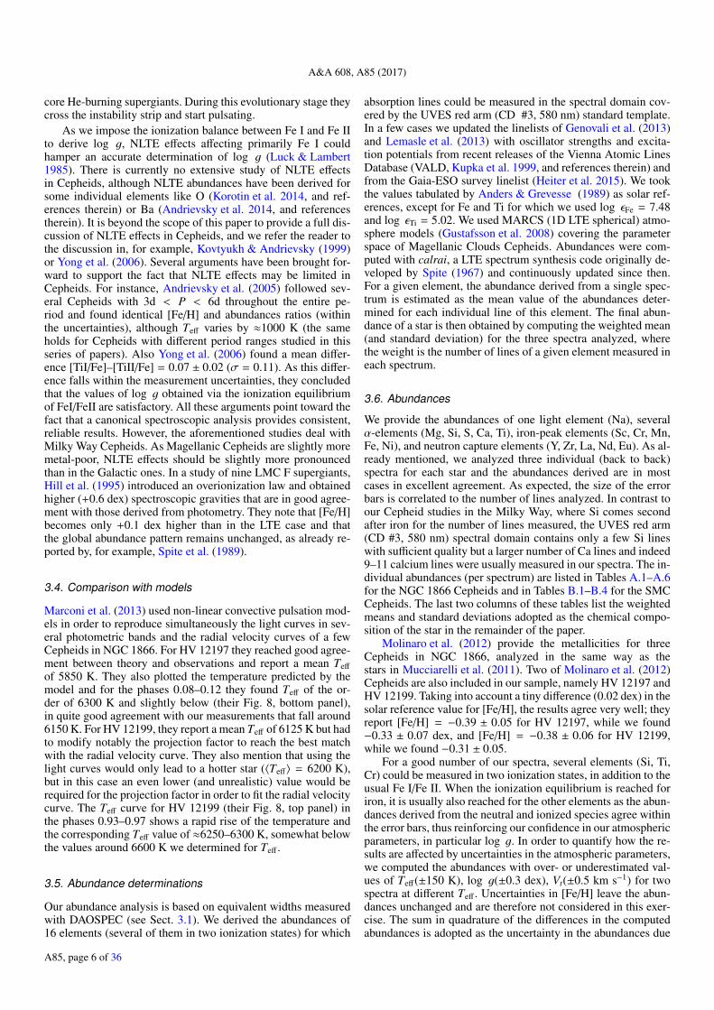
As we impose the ionization balance between Fe I and Fe IIto derive log g, NLTE effects affecting primarily Fe I couldhamper an accurate determination of log g (Luck & Lambert1985). There is currently no extensive study of NLTE effectsin Cepheids, although NLTE abundances have been derived forsome individual elements like O (Korotin et al. 2014, and ref-erences therein) or Ba (Andrievsky et al. 2014, and referencestherein). It is beyond the scope of this paper to provide a full dis-cussion of NLTE effects in Cepheids, and we refer the reader tothe discussion in, for example, Kovtyukh & Andrievsky (1999)or Yong et al. (2006). Several arguments have been brought for-ward to support the fact that NLTE effects may be limited inCepheids. For instance, Andrievsky et al. (2005) followed sev-eral Cepheids with 3d < P < 6d throughout the entire pe-riod and found identical [Fe/H] and abundances ratios (withinthe uncertainties), although Teff varies by ≈1000 K (the sameholds for Cepheids with different period ranges studied in thisseries of papers). Also Yong et al. (2006) found a mean differ-ence [TiI/Fe]–[TiII/Fe] = 0.07 ± 0.02 (σ = 0.11). As this differ-ence falls within the measurement uncertainties, they concludedthat the values of log g obtained via the ionization equilibriumof FeI/FeII are satisfactory. All these arguments point toward thefact that a canonical spectroscopic analysis provides consistent,reliable results. However, the aforementioned studies deal withMilky Way Cepheids. As Magellanic Cepheids are slightly moremetal-poor, NLTE effects should be slightly more pronouncedthan in the Galactic ones. In a study of nine LMC F supergiants,Hill et al. (1995) introduced an overionization law and obtainedhigher (+0.6 dex) spectroscopic gravities that are in good agree-ment with those derived from photometry. They note that [Fe/H]becomes only +0.1 dex higher than in the LTE case and thatthe global abundance pattern remains unchanged, as already re-ported by, for example, Spite et al. (1989).

3.4. Comparison with models

Marconi et al. (2013) used non-linear convective pulsation mod-els in order to reproduce simultaneously the light curves in sev-eral photometric bands and the radial velocity curves of a fewCepheids in NGC 1866. For HV 12197 they reached good agree-ment between theory and observations and report a mean Teff

of 5850 K. They also plotted the temperature predicted by themodel and for the phases 0.08–0.12 they found Teff of the or-der of 6300 K and slightly below (their Fig. 8, bottom panel),in quite good agreement with our measurements that fall around6150 K. For HV 12199, they report a mean Teff of 6125 K but hadto modify notably the projection factor to reach the best matchwith the radial velocity curve. They also mention that using thelight curves would only lead to a hotter star (〈Teff〉 = 6200 K),but in this case an even lower (and unrealistic) value would berequired for the projection factor in order to fit the radial velocitycurve. The Teff curve for HV 12199 (their Fig. 8, top panel) inthe phases 0.93–0.97 shows a rapid rise of the temperature andthe corresponding Teff value of ≈6250–6300 K, somewhat belowthe values around 6600 K we determined for Teff .

3.5. Abundance determinations

Our abundance analysis is based on equivalent widths measuredwith DAOSPEC (see Sect. 3.1). We derived the abundances of16 elements (several of them in two ionization states) for which

absorption lines could be measured in the spectral domain cov-ered by the UVES red arm (CD #3, 580 nm) standard template.In a few cases we updated the linelists of Genovali et al. (2013)and Lemasle et al. (2013) with oscillator strengths and excita-tion potentials from recent releases of the Vienna Atomic LinesDatabase (VALD, Kupka et al. 1999, and references therein) andfrom the Gaia-ESO survey linelist (Heiter et al. 2015). We tookthe values tabulated by Anders & Grevesse (1989) as solar ref-erences, except for Fe and Ti for which we used log εFe = 7.48and log εTi = 5.02. We used MARCS (1D LTE spherical) atmo-sphere models (Gustafsson et al. 2008) covering the parameterspace of Magellanic Clouds Cepheids. Abundances were com-puted with calrai, a LTE spectrum synthesis code originally de-veloped by Spite (1967) and continuously updated since then.For a given element, the abundance derived from a single spec-trum is estimated as the mean value of the abundances deter-mined for each individual line of this element. The final abun-dance of a star is then obtained by computing the weighted mean(and standard deviation) for the three spectra analyzed, wherethe weight is the number of lines of a given element measured ineach spectrum.

3.6. Abundances

We provide the abundances of one light element (Na), severalα-elements (Mg, Si, S, Ca, Ti), iron-peak elements (Sc, Cr, Mn,Fe, Ni), and neutron capture elements (Y, Zr, La, Nd, Eu). As al-ready mentioned, we analyzed three individual (back to back)spectra for each star and the abundances derived are in mostcases in excellent agreement. As expected, the size of the errorbars is correlated to the number of lines analyzed. In contrast toour Cepheid studies in the Milky Way, where Si comes secondafter iron for the number of lines measured, the UVES red arm(CD #3, 580 nm) spectral domain contains only a few Si lineswith sufficient quality but a larger number of Ca lines and indeed9–11 calcium lines were usually measured in our spectra. The in-dividual abundances (per spectrum) are listed in Tables A.1–A.6for the NGC 1866 Cepheids and in Tables B.1–B.4 for the SMCCepheids. The last two columns of these tables list the weightedmeans and standard deviations adopted as the chemical compo-sition of the star in the remainder of the paper.

Molinaro et al. (2012) provide the metallicities for threeCepheids in NGC 1866, analyzed in the same way as thestars in Mucciarelli et al. (2011). Two of Molinaro et al. (2012)Cepheids are also included in our sample, namely HV 12197 andHV 12199. Taking into account a tiny difference (0.02 dex) in thesolar reference value for [Fe/H], the results agree very well; theyreport [Fe/H] = −0.39 ± 0.05 for HV 12197, while we found−0.33 ± 0.07 dex, and [Fe/H] = −0.38 ± 0.06 for HV 12199,while we found −0.31 ± 0.05.

For a good number of our spectra, several elements (Si, Ti,Cr) could be measured in two ionization states, in addition to theusual Fe I/Fe II. When the ionization equilibrium is reached foriron, it is usually also reached for the other elements as the abun-dances derived from the neutral and ionized species agree withinthe error bars, thus reinforcing our confidence in our atmosphericparameters, in particular log g. In order to quantify how the re-sults are affected by uncertainties in the atmospheric parameters,we computed the abundances with over- or underestimated val-ues of Teff(±150 K), log g(±0.3 dex), Vt(±0.5 km s−1) for twospectra at different Teff . Uncertainties in [Fe/H] leave the abun-dances unchanged and are therefore not considered in this exer-cise. The sum in quadrature of the differences in the computedabundances is adopted as the uncertainty in the abundances due

A85, page 6 of 36

B. Lemasle et al.: Detailed chemical composition of classical Cepheids in the Magellanic Clouds

Table 4. Uncertainties in the final abundances due to uncertainties inthe atmospheric parameters.

Error budget for HV 12198, φ = 0.675 (MJD = 54 806.13684767)Element ∆Teff ∆log g ∆Vt Quadratic

(±150 K) (±0.3 dex) (±0.5 km s−1) sum(dex) (dex) (dex) (dex)

[NaI/H] 0.08 0.00 0.03 0.09[MgI/H] 0.14 0.00 0.08 0.16[SiI/H] 0.07 0.01 0.03 0.07[SiII/H] 0.12 0.12 0.11 0.19[SI/H] 0.07 0.08 0.04 0.11

[CaI/H] 0.10 0.00 0.06 0.12[ScII/H] 0.03 0.12 0.08 0.15[TiI/H] 0.15 0.00 0.03 0.15[TiII/H] 0.02 0.12 0.02 0.12[CrII/H] 0.02 0.11 0.07 0.13[MnI/H] 0.12 0.00 0.03 0.12[FeI/H] 0.13 0.00 0.05 0.13[FeII/H] 0.01 0.12 0.05 0.13[NiI/H] 0.13 0.00 0.04 0.13[YII/H] 0.04 0.12 0.05 0.13[ZrII/H] 0.03 0.11 0.03 0.12[LaII/H] 0.07 0.12 0.04 0.14[NdII/H] 0.07 0.22 0.05 0.23[EuII/H] 0.04 0.12 0.02 0.12Error budget for HV 1328, φ = 0.884 (MJD = 54 785.02744873)Element ∆Teff ∆log g ∆Vt Quadratic

(±150 K) (±0.3 dex) (±0.5 km s−1) sum(dex) (dex) (dex) (dex)

[NaI/H] 0.10 0.04 0.02 0.11[MgI/H] 0.11 0.05 0.02 0.12[SiI/H] 0.18 0.07 0.02 0.19[CaI/H] 0.13 0.06 0.04 0.15[ScII/H] 0.28 0.10 0.06 0.30[TiI/H] 0.09 0.11 0.03 0.15[TiII/H] 0.12 0.03 0.07 0.14[CrI/H] 0.13 0.05 0.07 0.15[CrII/H] 0.10 0.07 0.06 0.13[FeI/H] 0.11 0.06 0.08 0.15[FeII/H] 0.22 0.13 0.09 0.26[NiI/H] 0.09 0.13 0.05 0.16[YII/H] 0.07 0.08 0.03 0.11[ZrII/H] 0.31 0.12 0.02 0.33[LaII/H] 0.13 0.05 0.03 0.14[NdII/H] 0.10 0.15 0.03 0.18[EuII/H] 0.28 0.08 0.03 0.29

Notes. Columns 2, 3, and 4 indicate how the abundances are modified(mean values) when they are computed with over- or underestimatedvalues of Teff(±150 K), log g(±0.3 dex), or Vt(±0.5 dex), respectively.The sum in quadrature of the differences is adopted as the uncertainty inthe abundances due to the uncertainties in the atmosphere parameters.

to the uncertainties in the atmosphere parameters. The resultingvalues are listed in Table 4.

For the stars in our sample, NLTE effects are negligible forNa (≤0.1 dex) as computed by Lind et al. (2011) for a rangeof atmospheric parameters including yellow supergiants and byTakeda et al. (2013) for Cepheids. Using DAOSPEC to auto-matically determine the EW of the lines (and the relativelylow S/N of our spectra) made it impossible for us to takeinto account the contribution of the hyperfine structure split-ting for iron-peak elements, and for neutron-capture elementsas in da Silva et al. (2016). Depending on the line considered,the latter authors estimated the hfs correction to range from

negligible to ≈0.20 dex. In the case of the 6262.29 La II line,it reaches −0.211± 0.178 dex, where the quoted error representsthe dispersion around the mean hfs correction for this line. Ina forthcoming paper (Lemasle et al., in prep.) we study the im-pact of the hfs on the Mn abundance in Milky Way Cepheids.The three Mn lines measured in our Magellanic Cepheids be-long to the (6013, 6016, 6021 Å) triplet and as expected we findlower Mn abundances when the hfs is taken into account. For the6013 Å lines, we find a mean effect of −0.18 ± 0.21 dex (max:−0.65 dex), while it is slightly lower for the 6016 and 6021 Ålines, with a mean effect of −0.12 ± 0.22 dex (max: −0.45 dex)and −0.12±0.16 dex (max: −0.40 dex), respectively. It should benoted that the Milky Way Cepheids are on average more metal-rich and somewhat cooler than the Magellanic Cepheids in oursample.

4. Discussion

4.1. The chemical composition of Cepheids in NGC 1866

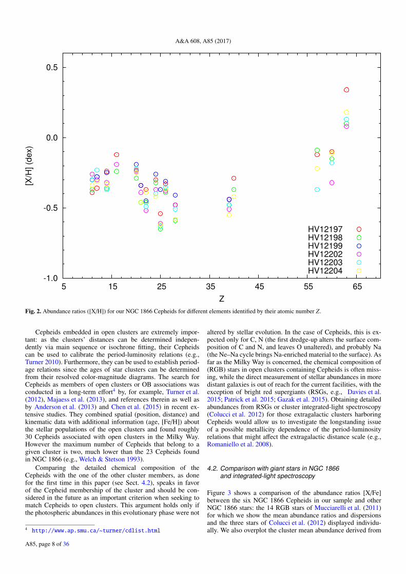
The most striking feature of the abundance pattern of theNGC 1866 Cepheids is the very low star-to-star scatter (seeFig. 2): all the elements for which a good number of lines couldbe measured (e.g., Si, Ca, Fe) have abundances [X/H] that fallwithin ≈0.1 dex of each other. The same also applies for otherelements (e.g., S, Sc, Ti, Ni, Y, Zr) where only a small numberof lines could be measured, and even in the case of, for example,Na or Mg, where only one line could be measured, the scatterremains smaller than 0.2 dex. In a few cases (mostly for neutron-capture elements), a star has a discrepant abundance for a givenelement, either because this element could be measured (proba-bly poorly) in only one of the spectra (e.g., Mn in HV 12199, Lain HV 12203) or because one of the spectra gives a discrepantvalue (e.g., Nd for HV 12202 or Eu for HV 12197). Ignoring theoutliers, the star to star scatter is similar to the one observed forthe other elements.

This small star-to-star scatter is a strong indication that thesix Cepheids in our NGC 1866 sample are genuine cluster mem-bers, sharing a very similar chemical composition as expected ifthey were born in the same place and at the same time. Indeed,they all have 2.64 d < P < 3.52 d and it is well-known that clas-sical Cepheids obey a period-age relation (e.g., Efremov 1978;Grebel & Brandner 1998; Bono et al. 2005, see also Sect. 4.3).

With [Fe/H] ≈ −0.4 dex, our NGC 1866 Cepheids can becompared to Cepheids located in the outer disc of the MilkyWay, at Galactocentric distances RG > 10 kpc. A quick glance atthe Cepheid abundances in, for example, Lemasle et al. (2013),and Genovali et al. (2015) indicates that the [Na/Fe] and [α/Fe]abundances in the NGC 1866 Cepheids fall slightly below thoseobserved in the Milky Way Cepheids for the corresponding rangeof metallicities. The same comparison for neutron-capture ele-ments (in da Silva et al. 2016) is less meaningful as the low S/Nof our spectra prevented us from taking the hyperfine structureinto account in the current study. The [Y/Fe] ratios appear to besimilar, which is not surprising as the hfs corrections reportedby da Silva et al. (2016) are small for the YII lines. The [La/Fe],[Nd/Fe], and [Eu/Fe] ratios appear to be higher than in the MilkyWay Cepheids with similar metallicities. This is certainly par-tially due to the hfs corrections. Indeed da Silva et al. (2016) re-port that the abundances derived from some of the La II lines canbe smaller by up to ≈0.2 dex. On the other hand, their hfs cor-rections for the Eu lines are very small, and they did not applyany correction for Nd, which indicates that at least a fraction ofthe difference is intrinsic.

A85, page 7 of 36

A&A 608, A85 (2017)

-1.0

-0.5

0.0

0.5

5 15 25 35 45 55 65

[X/H

] (d

ex)

Z

HV12197HV12198HV12199HV12202HV12203HV12204

Fig. 2. Abundance ratios ([X/H]) for our NGC 1866 Cepheids for different elements identified by their atomic number Z.

Cepheids embedded in open clusters are extremely impor-tant: as the clusters’ distances can be determined indepen-dently via main sequence or isochrone fitting, their Cepheidscan be used to calibrate the period-luminosity relations (e.g.,Turner 2010). Furthermore, they can be used to establish period-age relations since the ages of star clusters can be determinedfrom their resolved color-magnitude diagrams. The search forCepheids as members of open clusters or OB associations wasconducted in a long-term effort4 by, for example, Turner et al.(2012), Majaess et al. (2013), and references therein as well asby Anderson et al. (2013) and Chen et al. (2015) in recent ex-tensive studies. They combined spatial (position, distance) andkinematic data with additional information (age, [Fe/H]) aboutthe stellar populations of the open clusters and found roughly30 Cepheids associated with open clusters in the Milky Way.However the maximum number of Cepheids that belong to agiven cluster is two, much lower than the 23 Cepheids foundin NGC 1866 (e.g., Welch & Stetson 1993).

Comparing the detailed chemical composition of theCepheids with the one of the other cluster members, as donefor the first time in this paper (see Sect. 4.2), speaks in favorof the Cepheid membership of the cluster and should be con-sidered in the future as an important criterion when seeking tomatch Cepheids to open clusters. This argument holds only ifthe photospheric abundances in this evolutionary phase were not

4 http://www.ap.smu.ca/~turner/cdlist.html

altered by stellar evolution. In the case of Cepheids, this is ex-pected only for C, N (the first dredge-up alters the surface com-position of C and N, and leaves O unaltered), and probably Na(the Ne–Na cycle brings Na-enriched material to the surface). Asfar as the Milky Way is concerned, the chemical composition of(RGB) stars in open clusters containing Cepheids is often miss-ing, while the direct measurement of stellar abundances in moredistant galaxies is out of reach for the current facilities, with theexception of bright red supergiants (RSGs, e.g., Davies et al.2015; Patrick et al. 2015; Gazak et al. 2015). Obtaining detailedabundances from RSGs or cluster integrated-light spectroscopy(Colucci et al. 2012) for those extragalactic clusters harboringCepheids would allow us to investigate the longstanding issueof a possible metallicity dependence of the period-luminosityrelations that might affect the extragalactic distance scale (e.g.,Romaniello et al. 2008).

4.2. Comparison with giant stars in NGC 1866and integrated-light spectroscopy

Figure 3 shows a comparison of the abundance ratios [X/Fe]between the six NGC 1866 Cepheids in our sample and otherNGC 1866 stars: the 14 RGB stars of Mucciarelli et al. (2011)for which we show the mean abundance ratios and dispersionsand the three stars of Colucci et al. (2012) displayed individu-ally. We also overplot the cluster mean abundance derived from

A85, page 8 of 36

B. Lemasle et al.: Detailed chemical composition of classical Cepheids in the Magellanic Clouds

-1.0

-0.5

0.0

0.5

1.0

5 15 25 35 45 55 65

[X/F

e] (d

ex)

Z

Colucci 2012Colucci 2012 (ILS)

HV12197HV12198HV12199HV12202HV12203HV12204

Mucciarelli 2011

Fig. 3. Abundance ratios ([X/Fe]) in NGC 1866 for different elements identified by their atomic number Z. Our Cepheids are the colored opencircles, The mean value and dispersion for RGB stars in NGC 1866 from Mucciarelli et al. (2011) are given by the black triangle and solid line.Individual stellar abundances in NGC 1866 by Colucci & Bernstein (2012) are depicted by gray stars. The mean value and dispersion obtained byColucci & Bernstein (2012) via integrated-light spectroscopy are indicated by the gray triangle and dotted line. All the abundance ratios have beenrescaled to our solar reference values.

integrated-light spectroscopy by Colucci et al. (2012). All theabundances have been rescaled to our solar reference values.

Our Cepheids are slightly enriched in sodium with respectto the RGB stars of Mucciarelli et al. (2011). Similar Na over-abundances have already been reported in the Milky Way (e.g.,Genovali et al. 2015) when comparing Cepheids and field dwarfsin the thin and thick disc (Soubiran & Girard 2005). Althoughthis overabundance is probably partially due to NLTE effects(see Sect. 3.6), it has been proposed that it may be caused bymixing events that dredge up material enriched in Na via theNeNa cycle into the surface of the Cepheids (Sasselov 1986;Denissenkov 1994; Takeda et al. 2013). Similar Na overabun-dances have also been observed in RGB stars (e.g., da Silva et al.2015), reinforcing this hypothesis. It is interesting to note thatNa overabundances are relatively homogeneous in Cepheidsand do not depend on mass or period (Andrievsky et al. 2003;Kovtyukh et al. 2005; Takeda et al. 2013; Genovali et al. 2015).In contrast, da Silva et al. (2015) report a positive trend withmass for [Na/Fe] for RGB stars (which cover a shorter massrange).

The agreement is excellent for the α-elements Mg and Si,and to a lesser extent for Ca for which the Cepheid abundancesare slightly larger than in the RGB stars. The agreement is good

for Fe and excellent for Ni, the only two iron peak elements forwhich data are available for both RGB stars and Cepheids. Forour six Cepheids we find a mean [Fe/H] = −0.36 dex with adispersion of 0.03 dex. The 14 RGB stars in Mucciarelli et al.(2011) have an average [Fe/H] of −0.43 dex (to which one shouldadd 0.02 dex to take into account differences in the adopted solariron abundance) and a dispersion of 0.04 dex.

In contrast, the abundances of some neutron-capture ele-ments are quite discrepant between the two studies: Y and Zrare found significantly more abundant (by 0.25/0.40 dex respec-tively) than in Mucciarelli et al. (2011). Our abundances of Laagree only within the error bars whereas Nd and Eu abundancesare in excellent agreement with those reported by these authors.The hfs corrections reported by da Silva et al. (2016) are negligi-ble for Y and therefore cannot account for the difference. In con-trast, hfs corrections can reach −0.2 dex for several La lines, anda good agreement between both studies could be achieved if theywere taken into account. A possible explanation for these dis-crepancies could be that the transitions used to derive the abun-dances of these elements are associated with different ionizationstages. For instance, Allen & Barbuy (2006, their Fig. 13) de-rived lower Zr abundances from Zr I lines than from Zr II linesin the Barium stars they analyzed, possibly because ionized lines

A85, page 9 of 36

A&A 608, A85 (2017)

are the dominant species and therefore less affected by depar-tures from the LTE. In the end, their Zr II abundances span arange of 0.40 ≤ [Zr II/Fe] ≤ 1.60 while their Zr I abundances arefound in the −0.20 ≤ [Zr I/Fe] ≤ 1.45 range. Mucciarelli et al.(2011) do not provide their linelist but given the wavelengthrange of their spectra, it is likely that they used neutral lines. Un-fortunately, neutral lines for these elements are too weak and/orblended in the spectra of Cepheids and therefore cannot be mea-sured to test this hypothesis. Only the Zr I lines at 6134.58 and6143.25 Å, and the Y I line at 6435.05 Å could possibly be mea-sured in the most metal-rich Milky Way Cepheids, but they be-come too weak already at solar metallicity.

The abundance ratios derived by Mucciarelli et al. (2011) forNGC 1866 members are in very good agreement with the fieldRGB stars in the surroundings they analyzed. It is interesting tonote that the [La/Fe] and [Eu/Fe] ratios derived in NGC 1866by Mucciarelli et al. (2011) are in good agreement with otherLMC field RGB stars (e.g., Van der Swaelmen et al. 2013, andreferences therein), while their [Y/Fe] and [Zr/Fe] ratios fall atthe lower end of the LMC field stars distribution.

Y and Zr belong to the first peak of the s-process, while Laand Ce belong to the second peak of the s-process that is fa-vored when metal-poor AGB stars dominate the chemical en-richment (e.g., Cristallo et al. 2011). The large values of [La/Fe]and [Ce/Fe] demonstrate that the enrichment in heavy elementsis dominated by metal-poor AGB stars for both the Cepheidsand RGB stars in NGC 1866. Cepheids show higher Y and Zrabundances than RGB stars. If this difference turns out to bereal, it might hint that they experienced extra enrichment in lights-process elements from more metal-rich AGB stars.

Similar conclusions can be drawn when comparing theCepheid abundances with the stellar abundances derived byColucci & Bernstein (2012): the α-elements (except Ti) andthe iron-peak elements abundance ratios (with respect to iron)they obtained are very similar to those of the Cepheids, whiletheir abundance ratios for the n-capture elements are higherthan in the Cepheids, and even higher than those derived byMucciarelli et al. (2011). Colucci & Bernstein (2012) did notmeasure Mn in their NGC 1866 stellar sample. However, theyfound values ([Mn/Fe] ≈ −0.35 dex) slightly lower than ours([Mn/Fe] ≈ −0.25 dex) in the stars belonging to other youngLMC clusters. The Mn abundances reported by Mucciarelli et al.(2011) are also (much) lower than ours. This is almost certainlydue to the fact that both studies included hfs corrections for Mn,which are known to be very significant (e.g., Prochaska et al.2000). Because these ratios are lower than in Milky Way stars ofthe same metallicity, they proposed that the type Ia supernovaeyields of Mn are metallicity-dependent, as reported/modeled inother environments by, for example, McWilliam et al. (2003),Cescutti et al. (2008), and North et al. (2012).

In contrast, the abundance ratios they derived fromintegrated-light spectroscopy are almost always significantlylarger than those obtained for RGB stars by Mucciarelli et al.(2011) or for Cepheids (this study), or at least at the higher end.This might be due to the fact that the work by Colucci et al.based on integrated-light includes contributions of many differ-ent stellar types (and possibly contaminating field populations).This is nevertheless surprising because the integrated flux origi-nating from a young cluster such as NGC 1866 should be dom-inated by young supergiants, and one would therefore expect abetter match between the Cepheids and the integrated-light spec-troscopy abundance ratios.

4.3. Multiple stellar populations in NGC 1866

In a recent paper, Milone et al. (2017) reported the discovery ofa split main sequence (MS) and of an extended main sequenceturn-off in NGC 1866. These intriguing features have alreadybeen reported in many of the intermediate-age clusters in theMagellanic Clouds as well as for some of their young clusters(e.g., Bertelli et al. 2003; Glatt et al. 2008; Milone et al. 2013),although there is no agreement whether this is indeed due tomultiple stellar populations. The blue MS hosts roughly 1/3 of theMS stars, the remaining 2⁄3 belonging to a spatially more concen-trated red MS. Milone et al. (2017) rule out the possibility thatage variations can be solely responsible for the split of the MSin NGC 1866. Instead, the red MS is consistent with a ≈200 Myrold population of extremely fast-rotating stars (ω = 0.9ωc) whilethe blue MS is consistent with non-rotating stars of similar age,including a small fraction of even older stars. However, accord-ing to Milone et al. (2017) the upper blue MS can only be re-produced by a somewhat younger population (≈140 Myr old)accounting for roughly 15% of the total MS stars.

As the age range of Cepheids is similar to the one of theNGC 1866 MS stars, it is natural to examine how they fit inthe global picture of NGC 1866 drawn by Milone et al. (2017).These authors clearly state in their conclusion that the above in-terpretation should only be considered as a working hypothesisand our only intent here is to examine if Cepheids can shed somelight on this scenario.

It is possible to compute individual ages for Cepheidswith a period-age relation derived from pulsation models (e.g.,Bono et al. 2005). Because rotation brings fresh material to thecore during the MS hydrogen burning phase, fast-rotating starsof intermediate masses stay longer on the MS and therefore crossthe instability strip later than a non-rotating star. Including ro-tation in models then increases the ages of Cepheids by 50 to100%, depending on the period, as computed by Anderson et al.(2016). Following the prescriptions of Anderson et al. (2016) wederive ages for all the Cepheids known in NGC 1866: we usea period-age relation computed with models with average rota-tion (ω = 0.5ωc) and averaged over the second and third cross-ing of the instability strip. Periods are taken from Musella et al.(2016). In the absence of further information, we assume thatthey are fundamental pulsators, except for V5, V6, and V8, asMusella et al. (2016) report that their periods and light curves aretypical of first overtone pulsators. Even more importantly, theylie on the PL relations of first overtones. For comparison, wealso derive ages using the period-age relation from Bono et al.(2005), which was computed using non-rotating pulsation mod-els. Ages are listed in Table 5.

We first notice that in both cases the age spread is verylimited, thus reinforcing previous findings stating that there isno age variation within NGC 1866, or at least that Cepheidsall belong to the same sub-population. As expected, the agescalculated with the period-age relation from Bono et al. (2005)lead to younger Cepheids and therefore appear to be com-patible only with the 140 Myr old stars populating the up-per part of the blue main sequence. None of the period-agerelations by Bono et al. (2005) and Anderson et al. (2016) en-able us to compute individual error bars. Uncertainties on theages of the NGC 1866 Cepheids of the order of 25–30 Myrcan be derived by using the standard deviation of the period-age relation by Bono et al. (2005) as the error. However,given quoted error bars of 50% or more (Anderson et al.2016), an age of 200 Myr cannot be completely excluded.On the other hand, the ages computed with the period-age

A85, page 10 of 36

B. Lemasle et al.: Detailed chemical composition of classical Cepheids in the Magellanic Clouds

Table 5. Individual ages for Cepheids in NGC 1866 computed with theperiod-age relations of Bono et al. (2005) or Anderson et al. (2016) forfundamental pulsators, and the periods listed in Musella et al. (2016).

Cepheid Period Agea Ageb

(no rotation) (rotation: ω = 0.5ωc)(d) (Myr) (Myr)

V6c 1.9442620 114.5 258.7V8c 2.0070000 111.7 252.0V5c 2.0390710 110.3 248.7

HV 12199 2.6391600 120.6 222.7HV 12200 2.7249800 117.6 218.0

We 4 2.8603600 113.2 211.1WS 5 2.8978000 112.1 209.3New 2.9429300 110.8 207.1

HV 12203 2.9541100 110.4 206.6We 8 3.0398490 108.0 202.7We 3 3.0490400 107.7 202.3

WS 11 3.0533000 107.6 202.1We 2 3.0548500 107.6 202.1WS 9 3.0694500 107.2 201.4

V1 3.0845500 106.8 200.8HV 12202 3.1012000 106.3 200.0HV 12197 3.1437100 105.2 198.2

We 5 3.1745000 104.4 197.0We 7 3.2322700 102.9 194.6We 6 3.2899400 101.5 192.3

V4 3.3180000 100.9 191.3HV 12204 3.4388200 98.1 186.8

V7 3.4520700 97.8 186.3HV 12198 3.5228000 96.3 183.8

Notes. (a) Period-age relation from Bono et al. (2005). (b) Period-agerelation from Anderson et al. (2016). (c) Ages computed using period-age relations for first overtone pulsators.

relation including rotation from Anderson et al. (2016) corre-spond very well to the fast-rotating red MS population. How-ever the reader should keep in mind that ages should be di-rectly compared only when they are on the same scale, whichrequires that they were all calculated based on the samemodels.

Using evolutionary tracks computed with either canonical(no overshooting) or non-canonical (moderate overshooting) as-sumptions (but no rotation), Musella et al. (2016) favor an age of140 Myr. The location of the Cepheids, in between the theoreti-cal blue loops computed in each case, does not allow us to dis-criminate between the two overshooting hypotheses. Adopting acanonical overshooting and an older age of 180 Myr enables usto better fit the observed luminosities of the Cepheids, but thetheoretical blue loops are then too short to reach the Cepheids’locus in the CMD. Finally, using high-resolution integrated-lightspectroscopy and CMD-fitting techniques, Colucci et al. (2011)report a similar age of 130 Myr.

Ages of Cepheids, derived using period-age relations com-puted with either no rotation or an average rotation (ω =0.5ωc), do not allow us to confirm or rule out the hypothesisof Milone et al. (2017). Unfortunately, Anderson et al. (2016) donot provide period-age relations for fast-rotators (ω = 0.9ωc).As far as Cepheid ages are concerned, it is interesting to notethat the Cepheids in NGC 1866 match very well the peak of the

0.40.60.81.01.21.41.6RA (h)

75.0

74.5

74.0

73.5

73.0

72.5

72.0

71.5

71.0

Dec

(deg

)

817

824829

834

837

847

865

1365

1954

20642195

2209822

132813331335

OGLE-IVRomaniello+2008This study

Fig. 4. SMC Cepheids with known metallicities (red: this study; blue:Romaniello et al. (2008); SMC Cepheids in the OGLE-IV database areshown as gray dots).

age distribution for LMC field Cepheids, computed by Inno et al.(2015b) using new period-age relations (without rotation) atLMC metallicities.

4.4. The metallicity gradients from Cepheids in the SMC

The existence of a metallicity gradient across the SMC is a long-debated issue. Using large numbers of RGB stars, Carrera et al.(2008), Dobbie et al. (2014), and Parisi et al. (2016) report a ra-dial metallicity gradient (−0.075 ± 0.011 dex deg−1 vs. −0.08 ±0.02 dex deg−1 in the two latter studies) in the inner few de-grees of the SMC. In both cases, this effect is attributed tothe increasing fraction of younger, more metal-rich stars to-wards the SMC center. However, the presence of such a gradi-ent was not confirmed by C- and M-type AGB stars (Cioni et al.2009), populous clusters (e.g., Parisi et al. 2015, 2016, and refer-ences therein), or RR Lyrae studies (e.g., Haschke et al. 2012a;Deb et al. 2015; Skowron et al. 2016, and references therein).

The SMC is very elongated and tilted by more than 20◦ (e.g.,Haschke et al. 2012b; Subramanian et al. 2012; Nidever et al.2013). Moreover, old and young stellar populations have sig-nificantly different spatial distributions and orientations (e.g.,Haschke et al. 2012b; Jacyszyn-Dobrzeniecka et al. 2017). Re-cent studies using mid-infrared Spitzer data (Scowcroft et al.2016) or optical data from the OGLE IV experiment(Jacyszyn-Dobrzeniecka et al. 2016) clearly confirmed this com-plex shape. Our Cepheid abundances combined with those foundin the literature (Romaniello et al. 2008), and the possibility toderive accurate distances thanks to the period-luminosity rela-tions allow us to shed new light on the SMC metallicity distri-bution. For the first time, we are able to probe the metallicitygradient in the SMC young population in the “depth” direc-tion. As Cepheids are young stars, it should be noted that ourstudy only concerns the present-day abundance gradient, and assuch, the metal-rich end of the metallicity distribution function([Fe/H] > −0.90 dex). Moreover, our sample is small (17 stars)and does not contain stars in the inner few degrees of the SMCin an on-sky projection (see Fig. 4). For old populations tracedby RR Lyrae stars, no significant metallicity gradient was foundin the “depth” direction (Haschke et al. 2012a).

A85, page 11 of 36

A&A 608, A85 (2017)

Table 6. Individual distances, ages, and metallicities for SMC Cepheids.

Cepheid log P Agea Distance Distance Uncertainty on [Fe/H](d) (Myr) (MIR) (pc) (NIR) (pc) NIR distances (pc) (dex)

HV 817 1.277 212.4 57 502 55 636c 1136 –0.79HV 823 1.504 186.9 – 60 770b 964 –0.77HV 824 1.819 161.2 56 700 51 195c 957 –0.70HV 829 1.926 154.2 55 506 53 625c 964 –0.73HV 834 1.867 157.9 57 420 60 463c 1168 –0.60HV 837 1.631 175.5 60 752 57 692c 1033 –0.80HV 847 1.433 194.2 63 160 60 129b 1175 –0.72HV 865 1.523 185.2 54 586 58 401c 1018 –0.84

HV 1365 1.094 239.7 71 595 68 986b 1094 –0.79HV 1954 1.222 219.8 54 265 57 702b 1027 –0.73HV 2064 1.527 184.7 65 503 58 973c 1182 –0.61HV 2195 1.621 176.3 58 568 58 703c 1163 –0.64HV 2209 1.355 202.8 56 286 56 543b 1006 –0.62

HV 11211 1.330 205.8 54 140 53 884c 966 –0.80HV 822 1.224 219.6 67 447 64 428b 1022 –0.70

HV 1328 1.200 223.0 61 750 61 526b 976 –0.63HV 1333 1.212 221.2 69 244 69 002b 1094 –0.86HV 1335 1.158 229.3 69 493 68 231b 1214 –0.78

Notes. Metallicities from Romaniello et al. (2008) have been put on the same metallicity scale (by adding 0.03 dex to them) as our data. (a) Period-age relation from Bono et al. (2005). (b) Distance based on IRSF/SIRIUS near-infrared photometry (Kato et al. 2007). (c) Distance based on 2MASSnear-infrared photometry (Skrutskie et al. 2006).

50 55 60 65 70 75z (kpc) based on MIR photometry

50

55

60

65

70

75

z (k

pc) b

ased

on

NIR

phot

omet

ry Romaniello+2008This study

Fig. 5. Comparison of distances derived either from near-infrared orfrom mid-infrared photometry (red: this study; blue: Romaniello et al.2008). Typical uncertainties are shown in the top left corner.

Individual distance moduli for SMC Cepheids were com-puted using the [3.6] µm mean-light magnitudes tabulated byScowcroft et al. (2016) and the corresponding PL-relation in themid-infrared (MIR) established by the same authors. Combin-ing the extinction law of Indebetouw et al. (2005) with that ofCardelli et al. (1989), Monson et al. (2012) reported a total-to-selective extinction ratio of A[3.6]/E(B−V) = 0.203. We adoptedthe average color excess found by Scowcroft et al. (2016) forthe SMC: E(B − V) = 0.071 ± 0.004 mag, which leads toA[3.6] = 0.014 ± 0.001 mag. There is no MIR photometry avail-able for HV 822 and HV 823. For HV 822, we use the dis-tance of 67 441.4 pc derived by Groenewegen et al. (2013) via

the Baade-Wesselink method. The typical uncertainty on the in-dividual MIR distances is of the order of ±3 kpc (Scowcroft et al.2016).

For comparison purposes, we also computed distances basedon NIR photometry. For the Cepheids in the OGLE-IV database,we used near-infrared J, H and KS magnitudes from theIRSF/SIRIUS catalog (Kato et al. 2007) that were derived by us-ing the near-infrared light-curve templates of Inno et al. (2015a).Distances were computed using period-Wesenheit (PW) rela-tions calibrated on the entire SMC sample of fundamental modeCepheids (>2200; stars Inno et al., in prep.). Wesenheit indicesare reddening-free quantities by construction (Madore 1982). Weused the WHJK index as defined by Inno et al. (2016): WHJK =H–1.046 × (J − KS) which is minimally affected by the un-certainty in the reddening law (Inno et al. 2016). For stars thatare not in the OGLE-IV database, the same procedure wasadopted, except that the distances are derived from 2MASS(Skrutskie et al. 2006) single epoch data (with no template ap-plied). Individual uncertainties on distances are listed in Table 6.The typical uncertainty, computed as the average of the individ-ual uncertainties, is 993 ± 41 pc and can be rounded to 1 kpc. It isbeyond the scope of this paper to compare both sets of distances.We simply mention here that they are in very good agreementdespite some star-to-star scatter (see Fig. 5).

To investigate the metallicity gradient in the SMC, we com-bine our [Fe/H] abundances with those of Romaniello et al.(2008), to which we added 0.03 dex to take into account differ-ences in the solar reference values. The Cepheids were placedin a Cartesian coordinate system using the transformationsof van der Marel & Cioni (2001) and Weinberg & Nikolaev(2001). We adopted the value tabulated in SIMBAD for the cen-ter of the SMC: α0 = 00h52m38.0s, δ0 = −72d48m01.00s(J2000). For the SMC distance modulus, we adopted thevalue reported by Graczyk et al. (2014) using eclipsing binaries:18.965 ± 0.025 (stat.) ± 0.048 (syst.) mag which translates into a

A85, page 12 of 36

B. Lemasle et al.: Detailed chemical composition of classical Cepheids in the Magellanic Clouds

Fig. 6. Metallicity distribution of SMC Cepheids in Cartesian coordinates. Distances are based on mid-infrared photometry.

distance of 62.1 ± 1.9 kpc. Individual distances and abundancescan be found in Table 6, as well as ages derived with the period-age relation of Bono et al. (2005).

A first glance at Fig. 6 shows that the (x, y) plane is notvery relevant because it does not reflect the depth of the SMC.This fact is reinforced in the case of Cepheids as they are brightstars that can be easily identified and analyzed, even at verylarge distances. More interesting are the (x, z) and especiallythe (y, z) plane, as they allow us to study, for the first time,the metallicity distribution of Cepheids along the SMC maincomponent. Our 17 Cepheids adequately sample the z direc-tion, but the reader should keep in mind that most of our tar-gets are located above the main body of the SMC (see Fig. 4 orJacyszyn-Dobrzeniecka et al. 2016, their Fig. 16). Figures 6 and7, where [Fe/H] is plotted as a function of z, show no evidenceof a metallicity gradient along the main axis of the SMC. Themetallicity spread barely reaches 0.3 dex, but both ends of thez-axis seem to be slightly more metal poor than the inner regionsas they miss the more metal-rich Cepheids. The age range spansonly 100 Myr and we see no correlation between age and metal-licity or distance. These interesting findings should neverthelessonly be considered as preliminary results, given the small size

of our sample and the location of our Cepheids outside the mainbody of the SMC.

5. Conclusions

In this paper we conduct a spectroscopic analysis of Cepheidsin the LMC and in the SMC. We provide abundances for a goodnumber of α, iron-peak, and neutron-capture elements. Our sam-ple increases by 20% (respectively 25%) the number of Cepheidswith known metallicities and by 46% (respectively 50%) thenumber of Cepheids with detailed chemical composition in thesegalaxies.

For the first time, we study the chemical composition of sev-eral Cepheids located in the same populous cluster NGC 1866,in the LMC. We find that the six Cepheids in our sample havea very homogeneous chemical composition, which is also con-sistent with RGB stars already analyzed in this cluster. Our re-sults are also in good agreement with theoretical models ac-counting for luminosity and radial velocity variations for the twostars (HV 12197, HV 12199) for which such measurements areavailable. Using various versions of period–age relations with no(ω = 0) or average rotation (ω = 0.5ωc) we find a similar age for

A85, page 13 of 36

A&A 608, A85 (2017)

50 55 60 65 70 75z (kpc) (MIR)

1.0

0.9

0.8

0.7

0.6

0.5

[Fe/

H] (d

ex)

Romaniello+2008This study

50 55 60 65 70 75z (kpc) (NIR)

1.0

0.9

0.8

0.7

0.6

0.5

[Fe/

H] (d

ex)

Romaniello+2008This study

Fig. 7. SMC metallicity distribution from Cepheids in the z (depth)direction. Top panel: distances derived from mid-infrared photometry;Bottom panel: distances derived from near-infrared photometry. Typicalerror bars are shown in the top left corner.

all the Cepheids in NGC 1866, indicating that they all belong tothe same stellar population.

Using near- or mid-infrared photometry and period-luminosity relations (Inno et al. 2016; Scowcroft et al. 2016),we compute the distances for Cepheids in the SMC. Combin-ing our abundances for Cepheids in the SMC with those ofRomaniello et al. (2008), we study for the first time the metallic-ity distribution of the young population in the SMC in the depthdirection. We find no metallicity gradient in the SMC, but ourdata include only a small number of stars and do not containCepheids in the inner few degrees of the SMC.

Acknowledgements. The authors would like to thank the referee, M. Van derSwaelmen, for his careful reading of the manuscript and for his valuable com-ments, which helped to improve the quality of this paper. This work was sup-ported by Sonderforschungsbereich SFB 881 The Milky Way System (subpro-ject A5) of the German Research Foundation (DFG). G.F. has been supportedby the Futuro in Ricerca 2013 (grant RBFR13J716). This work has made use ofthe VALD database, operated at Uppsala University, the Institute of AstronomyRAS in Moscow, and the University of Vienna.

ReferencesAllen, D. M., & Barbuy, B. 2006, A&A, 454, 895Anders, E., & Grevesse, N. 1989, Geochim. Cosmochim. Acta, 53, 1976Anderson, R. I. 2014, A&A, 566, L10Anderson, R. I., Eyer, L., & Mowlavi, N. 2013, MNRAS, 434, 2238Anderson, R. I., Saio, H., Ekström, S., Georgy, C., & Meynet, G. 2016, A&A,

591, A8Andrievsky, S. M., Kovtyukh, V. V., Luck, R. E., et al. 2002a, A&A, 381, 32Andrievsky, S. M., Bersier, D., Kovtyukh, V. V., et al. 2002b, A&A, 384, 140Andrievsky, S. M., Egorova, I. A., Korotin, S. A., & Kovtyukh, V. V. 2003,

Astron. Nachr., 324, 532Andrievsky, S. M., Luck, R. E., & Kovtyukh, V. V. 2005, AJ, 130, 1880Andrievsky, S. M., Luck, R. E., & Korotin, S. A. 2014, MNRAS, 437, 2106Andrievsky, S. M., Martin, R. P., Kovtyukh, V. V., Korotin, S. A., & Lépine, J.

R. D. 2016, MNRAS, 461, 4256Barnes, T. G., & Evans, D. S. 1976, MNRAS, 174, 489Benedict, G. F., McArthur, B. E., Feast, M. W., et al. 2007, AJ, 133, 1810Bertelli, G., Nasi, E., Girardi, L., et al. 2003, AJ, 125, 770Bhardwaj, A., Kanbur, S. M., Macri, L. M., et al. 2016, AJ, 151, 88Bono, G., & Marconi, M. 1997, MNRAS, 290, 353Bono, G., Marconi, M., Cassisi, S., et al. 2005, ApJ, 621, 966Bono, G., Caputo, F., Marconi, M., & Musella, I. 2010, ApJ, 715, 277Breitfelder, J., Mérand, A., Kervella, P., et al. 2016, A&A, 587, A117Brocato, E., Caputo, F., Castellani, V., Marconi, M., & Musella, I. 2004, AJ, 128,

1597Cardelli, J. A., Clayton, G. C., & Mathis, J. S. 1989, ApJ, 345, 245Carrera, R., Gallart, C., Aparicio, A., et al. 2008, AJ, 136, 1039,Cescutti, G., Matteucci, F., Lanfranchi, G. A., & McWilliam, A. 2008, A&A,

491, 401Chen, X., de Grijs, R., & Deng, L. 2015, MNRAS, 446, 1268Cioni, M.-R. L. 2009, A&A, 506, 1137Colucci, J. E., & Bernstein, R. A. 2012, ApJ, 749, 124Colucci, J. E., Bernstein, R. A., Cameron, S. A., & McWilliam, A. 2011, ApJ,

735, 55Colucci, J. E., Bernstein, R. A., Cameron, S. A., & McWilliam, A. 2012, ApJ,

746, 29Cristallo, S., Piersanti, L., Straniero, O., et al. 2011, ApJS, 197, 17da Silva, R., Milone, A. C., & Rocha-Pinto, H. J. 2015, A&A, 580, A24da Silva, R., Lemasle, B., Bono, G., et al. 2016, A&A, 586, A125Davies, B., Kudritzki, R.-P., Gazak, Z., et al. 2015, ApJ, 806, 21Deb, S., Singh, H. P., Kumar, S., & Kanbur, S. M. 2015, MNRAS, 449, 2768Dekker, H., D’Odorico, S., Kaufer, A., Delabre, B., & Kotzlowski, H. 2000, Proc.

SPIE, 4008, 534Denissenkov, P. A. 1994, A&A, 287, 113Dobbie, P. D., Cole, A. A., Subramaniam, A., & Keller, S. 2014, MNRAS, 442,

1680Efremov, Iu. N. 1978, Soviet. Astron., 22, 161Feast, M. W., Whitelock, P. A., Menzies, J. W., & Matsunaga, N. 2012, MNRAS,

421, 2998Fiorentino, G., Marconi, M., Musella, I., & Caputo, F. 2007, A&A, 476, 863Fouqué, P., & Gieren, W. P. 1997, A&A, 320, 799Fouqué, P., Arriagada, P., Storm, J., et al. 2007, A&A, 476, 73Freudling, W., Romaniello, M., Bramich, D. M., et al. 2013, A&A, 559, A96Gazak, J. Z., Kudritzki, R., Evans, C., et al. 2015, ApJ, 805, 182Genovali, K., Lemasle, B., Bono, G., et al. 2013, A&A, 554, A132Genovali, K., Lemasle, B., Bono, G., et al. 2014, A&A, 566, A37Genovali, K., Lemasle, B., da Silva, R., et al. 2015, A&A, 580, A17Gieren, W., Storm, J., Barnes, T., G., III, et al. 2005, ApJ, 627, 224Gieren, W., Górski, M., Pietrzynski, G., et al. 2013, ApJ, 773, 69Glatt, K., Grebel, E. K., Sabbi, E., et al. 2008, AJ, 136, 1703Graczyk, D., Pietrzy/’nski, G., Thompson, I. B., et al. 2014, ApJ, 780, 59Grebel, E. K., & Brandner, W. 1998, in Magellanic Clouds and Other Dwarf

Galaxies, eds. T. Richtler, & J. M. Braun (Aachen: Shaker Verlag), 151Groenewegen, M. A. T. 2008, A&A, 488, 25Groenewegen, M. A. T. 2013, A&A, 550, 70Gustafsson, B., Edvardsson, B., Eriksson, K., et al. 2008, A&A, 486, 951Haschke, R., Grebel, E. K., & Duffau, S. 2012a, AJ, 143, 48Haschke, R., Grebel, E. K., & Duffau, S. 2012b, AJ, 144, 107Heiter, U., Lind, K., Asplund, M., et al. 2015, Phys. Scr., 90, 054010Hill, V., Andrievsky, S. M., & Spite, M. 1995, A&A, 293, 347Hill, V., François, P., Spite, M., Primas, F., & Spite, F. 2000, A&A, 364, 19Indebetouw, R., Mathis, J. S., Babler, B. L., et al. 2005, ApJ, 619, 931Inno, L., Matsunaga, N., Bono, G., et al. 2013, ApJ, 764, 84Inno, L., Matsunaga, N., Romaniello, M., et al. 2015a, A&A, 576, A30Inno, L., Bono, G., Romaniello, M., et al. 2015b, ASP Conf., 491, 265Inno, L., Bono, G., Matsunaga, N., et al. 2016, ApJ, 832, 176

A85, page 14 of 36

B. Lemasle et al.: Detailed chemical composition of classical Cepheids in the Magellanic Clouds

Jacyszyn-Dobrzeniecka, A. M., Skowron, D. M., Mróz, P., et al. 2016, ActaAstron., 66, 149

Jacyszyn-Dobrzeniecka, A. M., Skowron, D. M., Mróz, P., et al. 2017, ActaAstron., 67, 1

Kato, D., Nagashima, C., Nagayama, T., et al. 2007, PASJ, 59, 6150Kervella, P., Nardetto, N., Bersier, D., Mourard, D., & Coudé du Foresto, V.

2004, A&A, 416, 941Kervella, P., Trahin, B., Bond, H. E., et al. 2017, A&A, 600, A127Kewley, L. J., & Ellison, S. L. 2008, ApJ, 681, 1183Korotin, S. A., Andrievsky, S. M., Luck, R. E., et al. 2014, MNRAS, 444, 3301Kovtyukh, V. V., & Andrievsky, S. M. 1999, A&A, 351, 597Kovtyukh, V. V., & Gorlova, N. I. 2000, A&A, 358, 587Kovtyukh, V. V., Wallerstein, G., & Andrievsky, S. M. 2005, PASP, 117, 1173Kupka, F., Piskunov, N. E., Ryabchikova, T. A., Stempels, H. C., & Weiss, W.

W. 1999, A&AS, 138, 119Lemasle, B., François, P., Bono, G., et al. 2007, A&A, 467, 283Lemasle, B., François, P., Piersimoni, A., et al. 2008, A&A, 490, 613Lemasle, B., François, P., Genovali, K., et al. 2013, A&A, 558, A31Lind, K., Asplund, M., Barklem, P. S., & Belyaev, A. K. 2011, A&A, 528, 103Luck, R. E., & Lambert, D. L. 1985, ApJ, 298, 782Luck, R. E., & Lambert, D. L. 1992, ApJS, 79, 303Luck, R. E., & Lambert, D. L. 2011, AJ, 142, 136Luck, R. E., Moffett, T. J., Barnes, III, T. G., & Gieren, W. P. 1998, AJ, 115, 605Luck, R. E., Gieren, W. P., Andrievsky, S. M., et al. 2003, A&A, 401, 939Luck, R. E., Andrievsky, S. M., Kovtyukh, V. V., Gieren, W., & Graczyk, D.

2011, AJ, 142, 51Madore, B. F. 1982, ApJ, 253, 575Majaess, D., Carraro, G., Moni Bidin, C., et al. 2013, A&A, 560, A22Marconi, M., Molinaro, R., Ripepi, V., Musella, I., & Brocato, E. 2013, MNRAS,

428, 2185Marconi, M., Molinaro, R., Ripepi, V., et al. 2017, MNRAS, 466, 3206Martin, R. P., Andrievsky, S. M., Kovtyukh, V. V., et al. 2015, MNRAS, 449,

4071McWilliam, A., Rich, R. M., & Smecker-Hane, T. A. 2003, ApJ, 592, L21Mérand, A., Kervella, P., Breitfelder, J., et al. 2015, A&A, 584, A80Milone, A. P., Bedin, L. R., Cassisi, S., et al. 2013, A&A, 555, A143Milone, A. P., Marino, A. F., D’Antona, F., et al. 2017, MNRAS, 465, 4363Molinaro, R., Ripepi, V., Marconi, M., et al. 2012, ApJ, 748, 69Monson, A. J., Freedman, W. L., Madore, B. F., et al. 2012, ApJ, 759, 146Mourard, D., Bonneau, D., Koechlin, L., et al. 1997, A&A, 317, 789Mucciarelli, A., Cristallo, S., Brocato, E., et al. 2011, MNRAS, 413, 837Musella, I., Marconi, M., Stetson, P. B., et al. 2016, MNRAS, 457, 3084Nardetto, N., Fokin, A., Fouqué, P., et al. 2011, A&A, 534, L16Nardetto, N., Poretti, E., Rainer, M., et al. 2014, A&A, 561, A151Neilson, H. R., Nardetto, N., Ngeow, C.-C., Fouqué, P., & Storm, J. 2012, A&A,

541, A134Ngeow, C.-C., Citro, D. M., & Kanbur, S. M. 2012, MNRAS, 420, 585Ngeow, C.-C., Sarkar, S., Bhardwaj, A., Kanbur, S. M., & Singh, H. P. 2015,

ApJ, 813, 57Nidever, D. L., Monachesi, A., Bell, E. F., et al. 2013, ApJ, 779, 145

North, P., Cescutti, G., Jablonka, P., et al. 2012, A&A, 541, A45Parisi, M. C., Geisler, D., Clariá, J. J., et al. 2015, AJ, 149, 154Parisi, M. C., Geisler, D., Carraro, G., et al. 2016, AJ, 152, 58Pasquini, L., Avila, G., Blecha, A., et al. 2002, The Messenger, 110, 1Patrick, L. R., Evans, C. J., Davies, B., et al. 2015, ApJ, 803, 14Pedicelli, S., Lemasle, B., Groenewegen, M., et al. 2010, A&A, 518, A11Pilyugin, L. S., & Grebel, E. K. 2016, MNRAS, 457, 3678Prochaska, J. X., Naumov, S. O., Carney, B. W., McWilliam, A., & Wolfe, A. M.

2000, AJ, 120, 2513Rich, J. A., Persson, S. E., Freedman, W. L., et al. 2014, ApJ, 794, 107Ripepi, V., Moretti, M. I., Marconi, M., et al. 2012, MNRAS, 424, 1807Romaniello, M., Primas, F., Mottini, M, et al. 2005, A&A, 429, 37Romaniello, M., Primas, F., Mottini, M., et al. 2008, A&A, 488, 731Sasselov, D. D. 1986, PASP, 98, 561Scowcroft, V., Freedman, W., L., Madore, B. F., et al. 2013, ApJ, 773, 106Scowcroft, V., Freedman, W., L., Madore, B. F., et al. 2016, ApJ, 816, 49SSkowron, D. M., Soszynski, I., Udalski, A., et al. 2016, Acta Astron., 66, 269Skrutskie, M. F., Cutri, R. M., Stiening, R., et al. 2006, AJ, 131, 1163Soszynski, I., Poleski, R., Udalski, A., et al. 2010, Acta Astron., 60, 17Soubiran, C., & Girard, P. 2005, A&A, 438, 139Spite, M. 1967, Ann. Astrophys., 30, 211Spite, F., Spite, M., & François, P. 1989, A&A, 210, 25Stetson, P. B., & Pancino, E. 2008, PASP, 120, 1332Storm, J., Carney, B. W., Gieren, W. P., et al. 2004a, A&A, 415, 521Storm, J., Carney, B. W., Gieren, W. P., et al. 2004b, A&A, 415, 531Storm, J., Gieren, W. P., Fouqué, P., Barnes, III, T. G., & Gómez, M. 2005, A&A,

440, 487Storm, J., Gieren, W., Fouqué, P., et al. 2011a, A&A, 534, A94Storm, J., Gieren, W., Fouqué, P., et al. 2011b, A&A, 534, A95Subramanian, S., & Subramaniam, A. 2012, ApJ, 744, 128Szabados, L. 2003, IBVS, 5394Szabados, L., & Nehz, D. 2012, MNRAS, 426, 3148Takeda, Y., Kang, D.-I., Han, I., Lee, B.-C., & Kim, K.-M. 2013, MNRAS, 432,

769Turner, D. G. 2010, Ap&SS, 326, 219Turner, D. G., Majaess, D. J., Lane, D. J., et al. 2012, MNRAS, 422, 2501Udalski, A., Szymanski, M. K., & Szymanski, G. 2015, Acta Astron., 65, 1van der Marel, R. P., & Cioni, M.-R. L. 2001, AJ, 122, 1807Van der Swaelmen, M., Hill, V., Primas, F., & Cole, A. A. 2013, A&A, 560,

A44van Leeuwen, F., Feast, M. W., Whitelock, P. A., & Laney, C. D. 2007, MNRAS,

379, 723Weinberg, M. D., & Nikolaev, S. 2001, ApJ, 548, 712Welch, D. L. 1994, AJ, 108, 1421Welch, D. L., & Stetson, P. B. 1993, AJ, 105, 1813Welch, D. L., Mateo, M., Côté, P., Fischer, P., & Madore, B. F. 1991, AJ, 101,

490Wesselink, A. J. 1969, MNRAS, 144, 297Yong, D., Carney, B. W., Teixera de Almeida, M. L., & Pohl, B. L. 2006, AJ,

131, 2256

A85, page 15 of 36

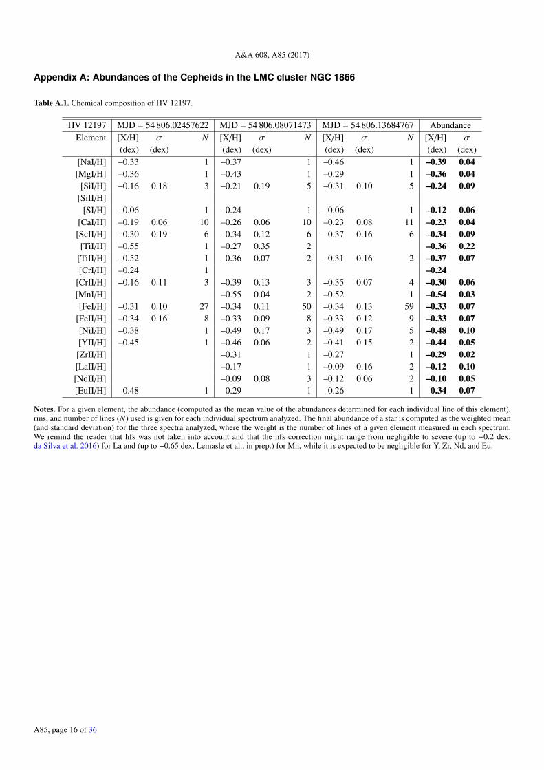
A&A 608, A85 (2017)

Appendix A: Abundances of the Cepheids in the LMC cluster NGC 1866

Table A.1. Chemical composition of HV 12197.

HV 12197 MJD = 54 806.02457622 MJD = 54 806.08071473 MJD = 54 806.13684767 AbundanceElement [X/H] σ N [X/H] σ N [X/H] σ N [X/H] σ

(dex) (dex) (dex) (dex) (dex) (dex) (dex) (dex)[NaI/H] –0.33 1 –0.37 1 –0.46 1 –0.39 0.04[MgI/H] –0.36 1 –0.43 1 –0.29 1 –0.36 0.04

[SiI/H] –0.16 0.18 3 –0.21 0.19 5 –0.31 0.10 5 –0.24 0.09[SiII/H]

[SI/H] –0.06 1 –0.24 1 –0.06 1 –0.12 0.06[CaI/H] –0.19 0.06 10 –0.26 0.06 10 –0.23 0.08 11 –0.23 0.04[ScII/H] –0.30 0.19 6 –0.34 0.12 6 –0.37 0.16 6 –0.34 0.09[TiI/H] –0.55 1 –0.27 0.35 2 –0.36 0.22

[TiII/H] –0.52 1 –0.36 0.07 2 –0.31 0.16 2 –0.37 0.07[CrI/H] –0.24 1 –0.24

[CrII/H] –0.16 0.11 3 –0.39 0.13 3 –0.35 0.07 4 –0.30 0.06[MnI/H] –0.55 0.04 2 –0.52 1 –0.54 0.03[FeI/H] –0.31 0.10 27 –0.34 0.11 50 –0.34 0.13 59 –0.33 0.07

[FeII/H] –0.34 0.16 8 –0.33 0.09 8 –0.33 0.12 9 –0.33 0.07[NiI/H] –0.38 1 –0.49 0.17 3 –0.49 0.17 5 –0.48 0.10[YII/H] –0.45 1 –0.46 0.06 2 –0.41 0.15 2 –0.44 0.05[ZrII/H] –0.31 1 –0.27 1 –0.29 0.02[LaII/H] –0.17 1 –0.09 0.16 2 –0.12 0.10[NdII/H] –0.09 0.08 3 –0.12 0.06 2 –0.10 0.05[EuII/H] 0.48 1 0.29 1 0.26 1 0.34 0.07

Notes. For a given element, the abundance (computed as the mean value of the abundances determined for each individual line of this element),rms, and number of lines (N) used is given for each individual spectrum analyzed. The final abundance of a star is computed as the weighted mean(and standard deviation) for the three spectra analyzed, where the weight is the number of lines of a given element measured in each spectrum.We remind the reader that hfs was not taken into account and that the hfs correction might range from negligible to severe (up to −0.2 dex;da Silva et al. 2016) for La and (up to −0.65 dex, Lemasle et al., in prep.) for Mn, while it is expected to be negligible for Y, Zr, Nd, and Eu.

A85, page 16 of 36

B. Lemasle et al.: Detailed chemical composition of classical Cepheids in the Magellanic Clouds

Table A.2. Same as Table A.1 for HV 12198.

HV 12198 MJD = 54 806.02457622 MJD = 54 806.08071473 MJD = 54 806.13684767 AbundanceElement [X/H] σ N [X/H] σ N [X/H] σ N [X/H] σ

(dex) (dex) (dex) (dex) (dex) (dex) (dex) (dex)[NaI/H] –0.37 0.05 2 –0.33 1 –0.40 0.13 2 –0.37 0.05[MgI/H] –0.34 1 –0.27 1 –0.23 1 –0.28 0.04

[SiI/H] –0.34 0.04 2 –0.31 0.28 5 –0.39 0.08 8 –0.36 0.09[SiII/H] –0.21 1 –0.27 1 –0.24 0.03

[SI/H] –0.24 1 –0.24[CaI/H] –0.35 0.14 3 –0.26 0.08 4 –0.26 0.05 3 –0.29 0.05[ScII/H] –0.50 0.06 2 –0.44 0.21 3 –0.44 0.10 3 –0.46 0.08[TiI/H] –0.43 1 –0.48 0.08 3 –0.46 0.15 3 –0.46 0.07

[TiII/H] –0.31 1 –0.34 1 –0.47 1 –0.37 0.05[CrI/H] –0.48 1 –0.48

[CrII/H] –0.23 0.17 2 –0.35 0.16 3 –0.34 0.09 3 –0.32 0.07[MnI/H] –0.64 0.05 2 –0.71 0.04 2 –0.57 1 –0.65 0.03[FeI/H] –0.39 0.10 33 –0.37 0.10 50 –0.40 0.07 43 –0.39 0.05

[FeII/H] –0.41 0.16 4 –0.38 0.11 5 –0.40 0.09 8 –0.40 0.06[NiI/H] –0.51 0.16 4 –0.59 0.16 6 –0.62 0.10 8 –0.59 0.07[YII/H] –0.38 0.13 2 –0.46 0.15 3 –0.57 0.15 3 –0.48 0.08[ZrII/H] –0.37 1 –0.37[LaII/H] –0.05 0.01 2 –0.07 0.03 2 –0.16 0.01 2 –0.09 0.02[NdII/H] –0.16 0.09 2 –0.15 0.05 3 –0.15 0.08 3 –0.15 0.04[EuII/H] 0.10 1 0.12 1 0.09 0.16 2 0.10 0.07

Table A.3. Same as Table A.1 for HV 12199.

HV 12199 MJD = 54 806.02457622 MJD = 54 806.08071473 MJD = 54 806.13684767 AbundanceElement [X/H] σ N [X/H] σ N [X/H] σ N [X/H] σ

(dex) (dex) (dex) (dex) (dex) (dex) (dex) (dex)[NaI/H] –0.33 1 –0.27 0.03 2 –0.31 0.01 2 –0.30 0.02[MgI/H] –0.26 1 –0.31 1 –0.27 1 –0.28 0.01

[SiI/H] –0.23 0.11 2 –0.31 0.05 3 –0.20 0.09 3 –0.25 0.04[SiII/H]

[SI/H][CaI/H] –0.17 0.12 10 –0.22 0.06 11 –0.17 0.11 11 –0.19 0.05[ScII/H] –0.32 0.21 3 –0.35 0.10 5 –0.34 0.11 6 –0.34 0.07[TiI/H] –0.47 1 –0.47

[TiII/H] –0.44 0.05 3 –0.48 0.03 2 –0.40 1 –0.45 0.03[CrI/H] –0.25 1 –0.36 1 –0.30 0.05

[CrII/H] –0.29 0.26 3 –0.16 0.08 2 –0.29 0.18 4 –0.26 0.11[MnI/H] –0.37 0.18 2 –0.37 0.18[FeI/H] –0.29 0.10 29 –0.30 0.05 35 –0.32 0.10 49 –0.31 0.05

[FeII/H] –0.30 0.09 8 –0.30 0.11 9 –0.31 0.15 11 –0.30 0.07[NiI/H] –0.33 0.15 3 –0.42 1 –0.53 0.06 2 –0.41 0.08[YII/H] –0.32 1 –0.48 1 –0.48 0.08 2 –0.44 0.05[ZrII/H][LaII/H][NdII/H][EuII/H]

A85, page 17 of 36

A&A 608, A85 (2017)

Table A.4. Same as Table A.1 for HV 12202.

HV 12202 MJD = 54 806.02457622 MJD = 54 806.08071473 MJD = 54 806.13684767 AbundanceElement [X/H] σ N [X/H] σ N [X/H] σ N [X/H] σ

(dex) (dex) (dex) (dex) (dex) (dex) (dex) (dex)[NaI/H] –0.31 1 –0.26 1 –0.23 0.06 2 –0.26 0.03[MgI/H] –0.28 1 –0.32 1 –0.30 1 –0.30 0.01

[SiI/H] –0.31 0.18 3 –0.31 0.14 4 –0.33 0.03 3 –0.32 0.07[SiII/H] –0.17 1 –0.17

[SI/H] –0.09 1 –0.29 1 –0.19 0.10[CaI/H] –0.35 0.13 9 –0.21 0.10 9 –0.17 0.08 9 –0.24 0.06[ScII/H] –0.45 0.23 3 –0.39 0.20 3 –0.30 0.03 2 –0.39 0.10[TiI/H] –0.68 1 –0.48 1 –0.40 1 –0.52 0.08

[TiII/H] –0.40 1 –0.40[CrI/H]

[CrII/H] –0.32 0.14 4 –0.40 0.19 3 –0.40 0.14 3 –0.37 0.08[MnI/H] –0.71 0.02 1 –0.58 0.03 3 –0.61 0.04[FeI/H] –0.38 0.08 29 –0.41 0.07 44 –0.36 0.10 41 –0.38 0.05

[FeII/H] –0.39 0.05 6 –0.40 0.15 5 –0.38 0.14 6 –0.39 0.06[NiI/H] –0.54 0.03 3 –0.53 0.08 2 –0.41 0.12 4 –0.48 0.06[YII/H] –0.40 0.01 –0.54 1 –0.58 1 –0.51 0.05[ZrII/H][LaII/H][NdII/H] –0.25 1 –0.39 1 –0.32 0.07[EuII/H] 0.08 1 0.08

Table A.5. Same as Table A.1 for HV 12203.

HV 12203 MJD = 54 806.02457622 MJD = 54 806.08071473 MJD = 54 806.13684767 AbundanceElement [X/H] σ N [X/H] σ N [X/H] σ N [X/H] σ

(dex) (dex) (dex) (dex) (dex) (dex) (dex) (dex)[NaI/H] –0.30 1 –0.30[MgI/H] –0.18 1 –0.18 1 –0.34 1 –0.23 0.05

[SiI/H] –0.28 0.12 3 –0.38 0.05 3 –0.41 0.10 5 –0.37 0.05[SiII/H] –0.23 1 –0.23

[SI/H][CaI/H] –0.25 0.13 4 –0.18 0.10 9 –0.25 0.12 6 –0.22 0.06[ScII/H] –0.33 0.22 5 –0.55 0.20 3 –0.57 0.02 3 –0.46 0.11[TiI/H] –0.46 1 –0.53 1 –0.49 0.04

[TiII/H][CrI/H]

[CrII/H] –0.25 0.33 2 –0.46 0.13 4 –0.42 0.22 3 –0.40 0.11[MnI/H] –0.71 1 –0.59 0.11 2 –0.64 0.06 2 –0.63 0.05[FeI/H] –0.33 0.14 32 –0.36 0.08 37 –0.36 0.12 45 –0.35 0.07

[FeII/H] –0.36 0.06 5 –0.39 0.11 2 –0.35 0.16 8 –0.36 0.09[NiI/H] –0.51 0.20 5 –0.45 0.06 3 –0.56 0.20 4 –0.51 0.10[YII/H] –0.34 0.19 2 –0.62 0.11 2 –0.49 0.11 2 –0.48 0.08[ZrII/H][LaII/H] –0.37 0.01 2 –0.37 0.01[NdII/H] –0.24 0.16 2 –0.12 0.13 2 –0.18 0.09[EuII/H] 0.13 0.06 2 0.13 0.06

A85, page 18 of 36

B. Lemasle et al.: Detailed chemical composition of classical Cepheids in the Magellanic Clouds

Table A.6. Same as Table A.1 for HV 12204.

HV 12204 MJD = 54 806.02457622 MJD = 54 806.08071473 MJD = 54 806.13684767 AbundanceElement [X/H] σ N [X/H] σ N [X/H] σ N [X/H] σ

(dex) (dex) (dex) (dex) (dex) (dex) (dex) (dex)[NaI/H] –0.37 0.08 2 –0.32 0.05 2 –0.34 1 –0.34 0.03[MgI/H] –0.34 1 –0.26 1 –0.32 1 –0.31 0.02

[SiI/H] –0.34 0.08 6 –0.36 0.02 6 –0.30 0.12 6 –0.33 0.05[SiII/H] –0.21 1 –0.18 1 –0.22 1 –0.20 0.01

[SI/H][CaI/H] –0.28 0.05 9 –0.21 0.07 10 –0.26 0.05 6 –0.25 0.03[ScII/H] –0.47 0.19 5 –0.47 0.15 6 –0.44 0.08 4 –0.46 0.08[TiI/H] –0.46 0.13 2 –0.42 0.11 3 –0.33 0.27 4 –0.39 0.12

[TiII/H] –0.64 1 –0.45 0.08 3 –0.43 0.06 3 –0.47 0.05[CrI/H] –0.56 1 –0.53 1 –0.55 0.02

[CrII/H] –0.47 0.06 2 –0.38 0.13 4 –0.46 0.28 2 –0.42 0.08[MnI/H] –0.64 1 –0.61 1 –0.60 1 –0.62 0.01[FeI/H] –0.38 0.07 44 –0.34 0.10 56 –0.38 0.10 57 –0.37 0.05

[FeII/H] –0.38 0.14 9 –0.35 0.09 10 –0.39 0.10 11 –0.37 0.06[NiI/H] –0.51 0.10 5 –0.60 0.10 7 –0.60 0.14 7 –0.58 0.07[YII/H] –0.54 0.02 3 –0.43 0.11 2 –0.62 0.09 4 –0.55 0.05[ZrII/H] –0.42 1 –0.43 1 –0.42 0.01[LaII/H] –0.17 1 –0.25 0.18 3 –0.21 0.15 5 –0.22 0.10[NdII/H] –0.06 0.26 2 –0.11 0.04 3 –0.15 0.02 3 –0.11 0.06[EuII/H] 0.18 1 0.18

A85, page 19 of 36

A&A 608, A85 (2017)

Appendix B: Abundances of the Cepheids in the SMC field

Table B.1. Same as Table A.1 for HV 822.

HV 822 MJD = 54 785.04026326 MJD = 54 785.05240828 MJD = 54 785.06455378 AbundanceElement [X/H] σ N [X/H] σ N [X/H] σ N [X/H] σ

(dex) (dex) (dex) (dex) (dex) (dex) (dex) (dex)[NaI/H] –0.90 1 –0.83 1 –0.86 0.04[MgI/H] –0.79 1 –0.75 1 –0.77 0.02

[SiI/H] –0.62 0.04 2 –0.67 0.13 3 –0.75 0.03 2 –0.68 0.05[SiII/H]

[SI/H] –0.54 1 –0.54[CaI/H] –0.52 0.15 9 –0.58 0.14 10 –0.59 0.13 9 –0.56 0.08[ScII/H] –0.96 0.18 6 –0.96 0.15 6 –1.00 0.18 5 –0.97 0.09[TiI/H]

[TiII/H] –0.80 0.21 4 –0.78 0.24 3 –0.80 0.21 3 –0.79 0.11[CrI/H] –0.66 1 –0.66

[CrII/H] –0.76 0.16 4 –0.77 0.13 4 –0.77 0.21 3 –0.77 0.09[MnI/H][FeI/H] –0.66 0.08 35 –0.71 0.06 31 –0.63 0.13 38 –0.66 0.06

[FeII/H] –0.72 0.12 12 –0.77 0.11 11 –0.74 0.09 11 –0.74 0.06[NiI/H] –0.82 1 –0.87 1 –0.84 0.03[YII/H] –1.18 1 –1.00 0.27 2 –1.06 0.17[ZrII/H] –0.73 1 –0.73[LaII/H][NdII/H][EuII/H]

A85, page 20 of 36

B. Lemasle et al.: Detailed chemical composition of classical Cepheids in the Magellanic Clouds

Table B.2. Same as Table A.1 for HV 1328.

HV 1328 MJD = 54 785.00779033 MJD = 54 785.01762254 MJD = 54 785.02744873 AbundanceElement [X/H] σ N [X/H] σ N [X/H] σ N [X/H] σ

(dex) (dex) (dex) (dex) (dex) (dex) (dex) (dex)[NaI/H] –0.79 1 –0.80 1 –0.79 1 –0.79 0.01[MgI/H] –0.70 1 –0.69 1 –0.71 1 –0.70 0.01

[SiI/H] –0.59 0.09 4 –0.68 0.14 2 –0.60 0.17 4 –0.61 0.07[SiII/H] –0.32 1 –0.32

[SI/H] –0.55 1 –0.55 1 –0.55[CaI/H] –0.58 0.07 10 –0.61 0.06 10 –0.64 0.05 10 –0.61 0.04[ScII/H] –0.66 0.17 5 –0.68 0.14 6 –0.71 0.16 4 –0.68 0.08[TiI/H] –0.76 1 –0.79 1 –0.83 1 –0.79 0.02

[TiII/H] –0.74 0.05 4 –0.67 0.08 4 –0.67 0.13 5 –0.69 0.06[CrI/H] –0.69 0.08 2 –0.69 0.08

[CrII/H] –0.54 0.11 2 –0.62 0.15 4 –0.63 0.15 4 –0.61 0.08[MnI/H] –0.85 1 –0.92 1 –0.89 0.04[FeI/H] –0.65 0.05 43 –0.66 0.08 47 –0.66 0.09 54 –0.66 0.05

[FeII/H] –0.62 0.07 11 –0.59 0.09 10 –0.60 0.10 12 –0.60 0.05[NiI/H] –1.00 0.06 2 –1.02 0.11 2 –1.01 0.05 2 –1.01 0.03[YII/H] –0.89 0.16 2 –0.87 0.14 2 –0.94 0.11 2 –0.90 0.06[ZrII/H] –0.66 1 –0.66 1 –0.70 1 –0.67 0.01[LaII/H] –0.21 1 –0.38 0.18 2 –0.32 0.12[NdII/H] –0.50 1 –0.47 1 –0.49 0.04 2 –0.49 0.02[EuII/H] –0.04 1 –0.08 1 –0.06 0.02

Table B.3. Same as Table A.1 for HV 1333.

HV 1333 MJD = 54 785.07912217 MJD = 54 785.09358357 MJD = 54 785.10804394 AbundanceElement [X/H] σ N [X/H] σ N [X/H] σ N [X/H] σ

(dex) (dex) (dex) (dex) (dex) (dex) (dex) (dex)[NaI/H] –0.95 1 –0.97 1 –0.96 0.01[MgI/H] –0.89 1 –0.67 1 –0.82 1 –0.79 0.06

[SiI/H] –0.88 0.10 4 –0.68 0.13 3 –0.79 0.08[SiII/H]

[SI/H][CaI/H] –0.81 0.09 8 –0.69 0.10 8 –0.82 0.12 8 –0.77 0.06[ScII/H] –0.96 0.10 2 –0.92 0.10 2 –0.81 1 –0.91 0.05[TiI/H] –1.00 0.08 2 –0.91 1 –0.97 0.06 2 –0.97 0.04

[TiII/H] –0.94 0.13 3 –0.83 0.20 3 –0.92 0.15 5 –0.90 0.09[CrI/H]

[CrII/H] –0.89 0.13 3 –0.92 0.16 4 –0.89 0.08 4 –0.90 0.07[MnI/H] –1.19 0.02 2 –1.15 1 –1.20 1 –1.18 0.02[FeI/H] –0.90 0.08 40 –0.80 0.05 34 –0.88 0.08 41 –0.86 0.04

[FeII/H] –0.88 0.10 10 –0.80 0.10 8 –0.89 0.12 7 –0.86 0.06[NiI/H] –1.09 0.15 4 –1.06 0.14 5 –1.09 0.15 4 –1.08 0.08[YII/H] –1.10 0.07 5 –1.01 0.08 4 –1.10 0.09 3 –1.07 0.04[ZrII/H] –0.76 1 –0.57 1 –0.71 1 –0.68 0.06[LaII/H] –0.78 0.24 3 –0.52 0.17 3 –0.54 0.08 3 –0.61 0.10[NdII/H] –0.50 0.13 3 –0.50 0.16 4 –0.49 0.10 3 –0.50 0.07[EuII/H] –0.36 1 –0.33 1 –0.34 0.01

A85, page 21 of 36

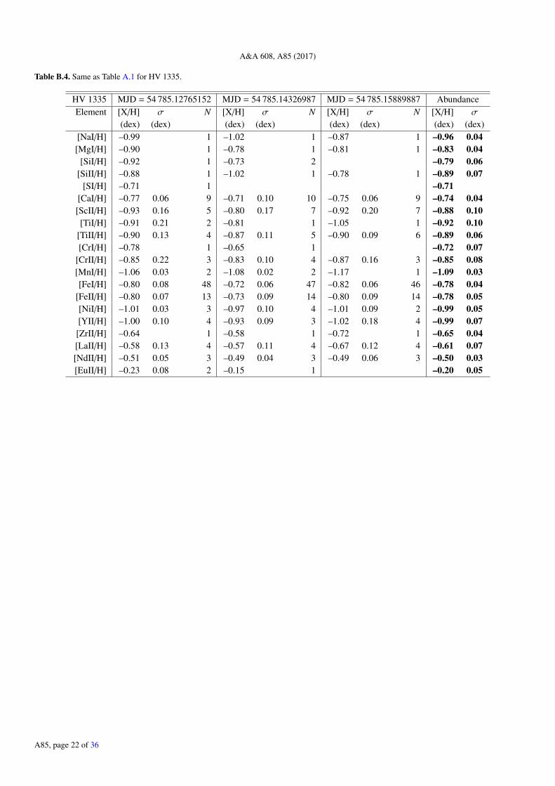
A&A 608, A85 (2017)

Table B.4. Same as Table A.1 for HV 1335.

HV 1335 MJD = 54 785.12765152 MJD = 54 785.14326987 MJD = 54 785.15889887 AbundanceElement [X/H] σ N [X/H] σ N [X/H] σ N [X/H] σ

(dex) (dex) (dex) (dex) (dex) (dex) (dex) (dex)[NaI/H] –0.99 1 –1.02 1 –0.87 1 –0.96 0.04[MgI/H] –0.90 1 –0.78 1 –0.81 1 –0.83 0.04

[SiI/H] –0.92 1 –0.73 2 –0.79 0.06[SiII/H] –0.88 1 –1.02 1 –0.78 1 –0.89 0.07

[SI/H] –0.71 1 –0.71[CaI/H] –0.77 0.06 9 –0.71 0.10 10 –0.75 0.06 9 –0.74 0.04[ScII/H] –0.93 0.16 5 –0.80 0.17 7 –0.92 0.20 7 –0.88 0.10[TiI/H] –0.91 0.21 2 –0.81 1 –1.05 1 –0.92 0.10

[TiII/H] –0.90 0.13 4 –0.87 0.11 5 –0.90 0.09 6 –0.89 0.06[CrI/H] –0.78 1 –0.65 1 –0.72 0.07

[CrII/H] –0.85 0.22 3 –0.83 0.10 4 –0.87 0.16 3 –0.85 0.08[MnI/H] –1.06 0.03 2 –1.08 0.02 2 –1.17 1 –1.09 0.03[FeI/H] –0.80 0.08 48 –0.72 0.06 47 –0.82 0.06 46 –0.78 0.04

[FeII/H] –0.80 0.07 13 –0.73 0.09 14 –0.80 0.09 14 –0.78 0.05[NiI/H] –1.01 0.03 3 –0.97 0.10 4 –1.01 0.09 2 –0.99 0.05[YII/H] –1.00 0.10 4 –0.93 0.09 3 –1.02 0.18 4 –0.99 0.07[ZrII/H] –0.64 1 –0.58 1 –0.72 1 –0.65 0.04[LaII/H] –0.58 0.13 4 –0.57 0.11 4 –0.67 0.12 4 –0.61 0.07[NdII/H] –0.51 0.05 3 –0.49 0.04 3 –0.49 0.06 3 –0.50 0.03[EuII/H] –0.23 0.08 2 –0.15 1 –0.20 0.05

A85, page 22 of 36

B. Lemasle et al.: Detailed chemical composition of classical Cepheids in the Magellanic Clouds

Appendix C: List of lines measured

Table C.1. Wavelengths (in Å) and atomic parameters of the spectral lines used in this study.

Wavelength Element chiex log g f Wavelength Element chiex log g f(Å) (eV) (Å) (eV)

4874.010 Ti2 3.09 –0.809 5627.497 Fe2 3.39 –4.104892.859 Fe1 4.22 –1.292 5633.946 Fe1 4.99 –0.234893.820 Fe2 2.83 –4.273 5638.262 Fe1 4.22 –0.774917.230 Fe1 4.19 –1.089 5641.000 Sc2 1.50 –1.134950.106 Fe1 3.42 –1.672 5641.434 Fe1 4.26 –1.084959.115 Nd2 0.06 –0.806 5645.613 Si1 4.93 –2.045005.157 Ti2 1.57 –2.737 5657.896 Sc2 1.51 –0.605017.570 Ni1 3.54 –0.024 5658.816 Fe1 3.40 –0.815044.211 Fe1 2.85 –2.045 5665.555 Si1 4.92 –1.945084.089 Ni1 3.68 –0.088 5667.149 Sc2 1.50 –1.315092.788 Nd2 0.38 –0.618 5669.042 Sc2 1.50 –1.205112.270 Zr2 1.66 –0.856 5679.023 Fe1 4.65 –0.825114.560 La2 0.23 –1.033 5682.633 Na1 2.10 –0.715119.112 Y2 0.99 –1.369 5684.202 Sc2 1.51 –1.075129.152 Ti2 1.89 –1.249 5686.530 Fe1 4.55 –0.665130.586 Nd2 1.30 0.450 5688.205 Na1 2.10 –0.405133.688 Fe1 4.18 0.148 5690.430 Si1 4.93 –1.775153.402 Na1 2.10 –1.740 5693.620 Fe1 4.96 –2.595155.125 Ni1 3.90 –0.560 5701.544 Fe1 2.56 –2.165155.762 Ni1 3.90 0.070 5705.464 Fe1 4.30 –1.355159.058 Fe1 4.28 –0.828 5708.400 Si1 4.95 –1.375176.559 Ni1 3.90 –0.300 5711.088 Mg1 4.34 –1.835196.059 Fe1 4.26 –0.496 5717.833 Fe1 4.28 –1.035210.385 Ti1 0.05 –0.835 5731.762 Fe1 4.26 –1.205216.274 Fe1 1.61 –2.081 5732.860 Fe1 4.10 –2.905217.389 Fe1 3.21 –1.121 5737.059 V1 1.06 –0.745305.853 Cr2 3.83 –2.363 5740.858 Nd2 1.16 –0.535307.361 Fe1 1.61 –2.911 5741.860 Fe1 4.26 –1.675329.138 Cr1 2.91 –0.061 5752.032 Fe1 4.55 –1.185329.990 Fe1 4.08 –1.198 5753.120 Fe1 4.26 –0.695334.869 Cr2 4.07 –1.617 5853.668 Ba2 0.60 –0.915336.771 Ti2 1.58 –1.638 5859.586 Fe1 4.55 –0.425345.796 Cr1 1.00 –0.950 5862.357 Fe1 4.55 –0.135349.465 Ca1 2.71 –0.311 5866.451 Ti1 1.07 –0.785353.370 Fe1 4.10 –0.840 5899.300 Ti1 1.05 –1.175369.961 Fe1 4.37 0.537 5905.671 Fe1 4.65 –0.695373.709 Fe1 4.47 –0.767 5909.973 Fe1 3.21 –2.595379.574 Fe1 3.69 –1.519 5916.247 Fe1 2.45 –2.915381.015 Ti2 1.57 –1.977 5927.789 Fe1 4.65 –0.995383.369 Fe1 4.31 0.641 5930.179 Fe1 4.65 –0.235398.279 Fe1 4.44 –0.634 5934.655 Fe1 3.93 –1.075402.774 Y2 1.84 –0.634 5948.541 Si1 5.08 –1.135410.910 Fe1 4.47 0.407 5956.694 Fe1 0.86 –4.55

A85, page 23 of 36

A&A 608, A85 (2017)

Table C.1. continued.

Wavelength Element chiex log g f Wavelength Element chiex log g f(Å) (eV) (Å) (eV)

5414.073 Fe2 3.22 –3.582 5976.777 Fe1 3.94 –1.245420.922 Cr2 3.76 –2.466 5983.680 Fe1 4.55 –1.475425.254 Fe1 1.01 –2.121 5984.815 Fe1 4.73 –0.205445.042 Fe1 4.39 –0.029 5987.065 Fe1 4.80 –0.435454.090 Ti2 1.57 –3.547 5991.376 Fe2 3.15 –3.655462.960 Fe1 4.47 –0.047 6003.011 Fe1 3.88 –1.125463.276 Fe1 4.43 0.073 6007.960 Fe1 4.65 –0.605501.465 Fe1 0.96 –3.056 6008.556 Fe1 3.88 –0.995502.067 Cr2 4.17 –2.097 6013.513 Mn1 3.07 –0.355509.895 Y2 0.99 –0.959 6016.673 Mn1 3.07 –0.185526.790 Sc2 1.77 0.027 6020.169 Fe1 4.61 –0.275528.405 Mg1 4.35 –0.625 6021.819 Mn1 3.08 –0.055572.842 Fe1 3.40 –0.270 6024.058 Fe1 4.55 –0.125576.089 Fe1 3.43 –0.903 6027.051 Fe1 4.08 –1.095581.965 Ca1 2.52 –0.552 6055.990 Fe1 4.73 –0.465590.114 Ca1 2.52 –0.572 6065.482 Fe1 2.61 –1.475591.370 Fe2 3.27 –4.597 6078.491 Fe1 4.80 –0.325601.277 Ca1 2.53 –0.523 6079.008 Fe1 4.65 –1.026082.710 Fe1 2.22 –3.57 6335.330 Fe1 2.20 –2.186084.111 Fe2 3.20 –3.88 6336.823 Fe1 3.69 –0.866085.270 Fe1 2.76 –2.86 6344.148 Fe1 2.43 –2.906091.919 Si1 5.87 –1.47 6347.109 Si2 8.12 0.176096.664 Fe1 3.98 –1.83 6355.028 Fe1 2.85 –2.326102.180 Fe1 4.84 –0.10 6358.697 Fe1 0.86 –4.476102.723 Ca1 1.88 –0.79 6362.338 Zn1 5.80 0.146108.107 Ni1 1.68 –2.44 6369.462 Fe2 2.89 –4.116113.322 Fe2 3.22 –4.23 6380.743 Fe1 4.19 –1.376122.217 Ca1 1.89 –0.32 6390.477 La2 0.32 –1.416127.906 Fe1 4.14 –1.40 6393.600 Fe1 2.43 –1.506141.713 Ba2 0.70 –0.03 6407.251 Fe2 3.89 –3.856149.258 Fe2 3.89 –2.84 6408.018 Fe1 3.69 –1.026151.617 Fe1 2.18 –3.31 6411.648 Fe1 3.65 –0.666155.134 Si1 5.62 –0.75 6414.980 Si1 5.87 –1.046157.728 Fe1 4.08 –1.16 6416.919 Fe2 3.89 –2.886160.747 Na1 2.10 –1.25 6419.980 Fe1 4.73 –0.176161.297 Ca1 2.52 –1.27 6421.350 Fe1 2.28 –2.026162.173 Ca1 1.90 –0.09 6430.845 Fe1 2.18 –1.986165.360 Fe1 4.14 –1.47 6432.680 Fe2 2.89 –3.576166.439 Ca1 2.52 –1.14 6433.457 Si1 5.96 –2.066169.042 Ca1 2.52 –0.80 6437.640 Eu2 1.32 –0.326169.563 Ca1 2.53 –0.48 6439.075 Ca1 2.52 0.396170.506 Fe1 4.79 –0.44 6449.808 Ca1 2.52 –0.506173.334 Fe1 2.22 –2.88 6455.598 Ca1 2.52 –1.296175.360 Ni1 4.09 –0.39 6462.567 Ca1 2.52 0.26

A85, page 24 of 36

B. Lemasle et al.: Detailed chemical composition of classical Cepheids in the Magellanic Clouds

Table C.1. continued.

Wavelength Element chiex log g f Wavelength Element chiex log g f(Å) (eV) (Å) (eV)

6176.807 Ni1 4.09 –0.26 6471.662 Ca1 2.53 –0.696180.203 Fe1 2.73 –2.62 6481.870 Fe1 2.28 –2.996187.989 Fe1 3.94 –1.62 6482.796 Ni1 1.93 –2.636191.558 Fe1 2.43 –1.42 6491.561 Ti2 2.06 –1.946200.313 Fe1 2.61 –2.40 6493.781 Ca1 2.52 –0.116213.430 Fe1 2.22 –2.48 6494.980 Fe1 2.40 –1.266215.150 Fe1 4.19 –1.14 6496.897 Ba2 0.60 –0.416216.354 V1 0.28 –1.29 6498.938 Fe1 0.96 –4.696219.281 Fe1 2.20 –2.43 6499.650 Ca1 2.52 –0.826229.226 Fe1 2.85 –2.80 6516.080 Fe2 2.89 –3.316230.722 Fe1 2.56 –1.28 6518.366 Fe1 2.83 –2.376232.640 Fe1 3.65 –1.22 6559.588 Ti2 2.05 –2.176237.319 Si1 5.61 –0.98 6569.214 Fe1 4.73 –0.386238.392 Fe2 3.89 –2.60 6572.779 Ca1 0.00 –4.246239.370 Fe2 2.81 –4.76 6586.308 Ni1 1.95 –2.756239.953 Fe2 3.89 –3.57 6592.913 Fe1 2.73 –1.476240.646 Fe1 2.22 –3.20 6593.870 Fe1 2.43 –2.396243.815 Si1 5.62 –1.24 6604.601 Sc2 1.36 –1.316244.466 Si1 5.62 –1.09 6606.949 Ti2 2.06 –2.806245.637 Sc2 1.51 –1.02 6609.110 Fe1 2.56 –2.686246.318 Fe1 3.60 –0.80 6613.733 Y2 1.75 –0.856247.557 Fe2 3.89 –2.43 6645.064 Eu2 1.38 0.126252.555 Fe1 2.40 –1.72 6677.990 Fe1 2.69 –1.376254.258 Fe1 2.28 –2.43 6680.133 Ti2 3.09 –1.796258.100 Ti1 1.44 –0.30 6680.140 Cr1 4.16 –0.396261.100 Ti1 1.43 –0.42 6703.566 Fe1 2.76 –3.066262.290 La2 0.40 –1.22 6715.410 Fe1 4.61 –1.366265.132 Fe1 2.18 –2.54 6717.681 Ca1 2.71 –0.526271.278 Fe1 3.33 –2.70 6721.848 Si1 5.86 –1.526279.753 Sc2 1.50 –1.25 6726.666 Fe1 4.61 –1.136290.965 Fe1 4.73 –0.77 6740.080 Nd2 0.06 –1.536297.793 Fe1 2.22 –2.70 6748.837 S1 7.87 –0.646301.500 Fe1 3.65 –0.72 6750.152 Fe1 2.42 –2.606318.018 Fe1 2.45 –1.80 6757.171 S1 7.87 –0.246318.717 Mg1 5.11 –2.10 6767.768 Ni1 1.83 –2.176320.410 La2 0.17 –1.33 6772.313 Ni1 3.66 –0.806320.851 Sc2 1.50 –1.82 6774.270 La2 0.13 –1.716322.685 Fe1 2.59 –2.45 6795.414 Y2 1.74 –1.036327.593 Ni1 1.68 –3.15

A85, page 25 of 36

A&A 608, A85 (2017)

Appendix D: Curves of growth

The curve of growth is a graph showing how the equivalent width (EW) of an absorption line varies with the abundance (A) ofthe atoms/ions producing the line. When there are few atoms, the line profile is dominated by Doppler broadening and EW ∝ A.When the line reaches saturation, EW ∝

√ln A. When saturation increases, the line profile becomes dominated by the wings due

to collisional broadening and EW ∝√

A.For weak lines it can be shown that log

(Wλ

λ

)varies linearly with log(α∗g f ). The Γ∗ quantity, defined as log

(Wλ

λ

)= log(α∗g f ) +

log Γ∗ can be computed for each individual line as a function of the atmosphere model, the element considered and its ionizationstage, the line excitation potential and so on. As the value of the stellar abundance α∗ is the unknown one wants to determine,the abundance of the same element in the Sun α� is used instead. The experimental curves of growth will then be shifted fromthe theoretical curves of growth by a factor log(α∗) − log(α�), which is by definition the abundance ratio [X/H] of the consideredelement X.

The experimental curve of growth is traced using many lines from the same element (e.g., Fe I) with a wide range of excitationpotentials and oscillator strengths that lead to a wide range of equivalent widths. The curves of growth plotted below show thetheoretical curves of growths computed for a line at λ = 5000 Å with χex = 3 and using the atmospheric parameters derived for thestar in the corresponding phase.

A85, page 26 of 36

B. Lemasle et al.: Detailed chemical composition of classical Cepheids in the Magellanic Clouds

(a)

(b)

(c)

(d)

(e)

(f)

Fig.

D.1

.Cur

ves

ofgr

owth

(Fe

I,Fe

II)f

orth

eH

V12

197

spec

tra.

From

left

tori

ght,

MJD

=54

806.

0245

7622

,54

806.

0807

1473

,54

806.

1368

4767

.

A85, page 27 of 36

A&A 608, A85 (2017)

(a)

(b)

(c)

(d)

(e)

(f)

Fig.

D.2

.Cur

ves

ofgr

owth

(Fe

I,Fe

II)f

orth

eH

V12

198

spec

tra.

From

left

tori

ght,

MJD

=54

806.

0245

7622

,54

806.

0807

1473

,54

806.

1368

4767

.

A85, page 28 of 36

B. Lemasle et al.: Detailed chemical composition of classical Cepheids in the Magellanic Clouds

(a)

(b)

(c)

(d)

(e)

(f)

Fig.

D.3

.Cur

ves

ofgr

owth

(Fe

I,Fe

II)f

orth

eH

V12

199

spec

tra.

From

left

tori

ght,

MJD

=54

806.

0245

7622

,54

806.

0807

1473

,54

806.

1368

4767

.

A85, page 29 of 36

A&A 608, A85 (2017)

(a)

(b)

(c)

(d)

(e)

(f)

Fig.

D.4

.Cur

ves

ofgr

owth

(Fe

I,Fe

II)f

orth

eH

V12

202

spec

tra.

From

left

tori

ght,

MJD

=54

806.

0245

7622

,54

806.

0807

1473

,54

806.

1368

4767

.

A85, page 30 of 36

B. Lemasle et al.: Detailed chemical composition of classical Cepheids in the Magellanic Clouds

(a)

(b)

(c)

(d)

(e)

(f)

Fig.

D.5

.Cur

ves

ofgr

owth

(Fe

I,Fe

II)f

orth

eH

V12

203

spec

tra.

From

left

tori

ght,

MJD

=54

806.

0245

7622

,54

806.

0807

1473

,54

806.

1368

4767

.

A85, page 31 of 36

A&A 608, A85 (2017)

(a)

(b)

(c)

(d)

(e)

(f)

Fig.

D.6

.Cur

ves

ofgr

owth

(Fe

I,Fe

II)f

orth

eH

V12

204

spec

tra.

From

left

tori

ght,

MJD

=54

806.

0245

7622

,54

806.

0807

1473

,54

806.

1368

4767

.

A85, page 32 of 36

B. Lemasle et al.: Detailed chemical composition of classical Cepheids in the Magellanic Clouds

(a)

(b)

(c)

(d)

(e)

(f)

Fig.

D.7

.Cur

ves

ofgr

owth

(Fe

I,Fe

II)f

orth

eH

V82

2sp

ectr

a.Fr

omle

ftto

righ

t,M

JD=

5478

5.04

0263

26,5

478

5.05

2408

28,5

478

5.06

4553

78.

A85, page 33 of 36

A&A 608, A85 (2017)

(a)

(b)

(c)

(d)

(e)

(f)

Fig.

D.8

.Cur

ves

ofgr

owth

(Fe

I,Fe

II)f

orth

eH

V13

28sp

ectr

a.Fr

omle

ftto

righ

t,M

JD=

5478

5.00

7790

33,5

478

5.01

7622

54,5

478

5.02

7448

73.

A85, page 34 of 36

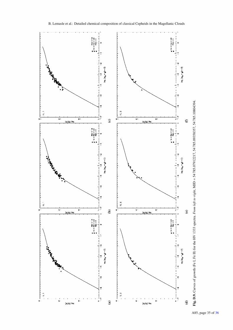
B. Lemasle et al.: Detailed chemical composition of classical Cepheids in the Magellanic Clouds

(a)

(b)

(c)

(d)

(e)

(f)

Fig.

D.9

.Cur

ves

ofgr

owth

(Fe

I,Fe

II)f

orth

eH

V13

33sp

ectr

a.Fr

omle

ftto

righ

t,M

JD=

5478

5.07

9122

17,5

478

5.09

3583

57,5

478

5.10

8043

94.

A85, page 35 of 36

A&A 608, A85 (2017)

(a)

(b)

(c)

(d)

(e)

(f)

Fig.

D.1

0.C

urve

sof

grow

th(F

eI,

FeII

)for

the

HV

1335

spec

tra.

From

left

tori

ght,

MJD

=54

785.

1276

5152

,54

785.

1432

6987

,54

785.

1588

9887

.

A85, page 36 of 36