NBER WORKING PAPER SERIES

ASSET LIQUIDITY AND THE COST OF CAPITAL

Hernán Ortiz-MolinaGordon M. Phillips

Working Paper 15992http://www.nber.org/papers/w15992

NATIONAL BUREAU OF ECONOMIC RESEARCH1050 Massachusetts Avenue

Cambridge, MA 02138May 2010

We thank Heitor Almeida, Murray Carlson, Jason Chen, Lorenzo Garlappi, Itay Goldstein (WFA discussant),N. R. Prabhala, Avri Ravid, Jason Schloetzer, as well as seminar participants at Georgetown University,the Pacific NorthWest Finance Conference 2008, and the Western Finance Association Meetings 2009for their helpful comments. Ortiz-Molina acknowledges the financial support from the Social Sciencesand Humanities Research Council of Canada. All errors are the authors alone. The views expressedherein are those of the authors and do not necessarily reflect the views of the National Bureau of EconomicResearch.

NBER working papers are circulated for discussion and comment purposes. They have not been peer-reviewed or been subject to the review by the NBER Board of Directors that accompanies officialNBER publications.

© 2010 by Hernán Ortiz-Molina and Gordon M. Phillips. All rights reserved. Short sections of text,not to exceed two paragraphs, may be quoted without explicit permission provided that full credit,including © notice, is given to the source.

Asset Liquidity and the Cost of CapitalHernán Ortiz-Molina and Gordon M. PhillipsNBER Working Paper No. 15992May 2010JEL No. G12,G32

ABSTRACT

We study the effect of real asset liquidity on a firm’s cost of capital. We find an aggregate asset-liquiditydiscount in firms’ cost of capital that is strongly counter-cyclical. At the firm-level we find that assetliquidity affects firms’ cost of capital both in the cross section and in the time series: Firms in industrieswith more liquid assets and during periods of high asset liquidity have lower cost of capital. This effectis stronger when the asset liquidity is provided by firms operating within the industry. We also findthat higher asset liquidity reduces the cost of capital by more for firms that face more competitiverisk in product markets, have less access to external capital or are closer to default, and for those facingnegative demand shocks. Our results suggest that asset liquidity is valuable to firms and, more generally,that operating inflexibility is an economically important source of risk.

Hernán Ortiz-MolinaSauder School of BusinessThe University of British Columbia2053 Main HallVancouver, BCCanada V6T 1Z2ortizmolina@sauder.ubc.ca

Gordon M. PhillipsR.H. Smith School of ManagementVan Munching HallUniversity of MarylandCollege Park, MD 20742and NBERgphillips@rhsmith.umd.edu

I. Introduction

Understanding what are the underlying sources of risk that drive the cross-sectional

and time-series variation in firms’ cost of capital is of fundamental interest in fi-

nancial economics. Previous work, including recent studies by Pástor, Sinha, and

Swaminathan (2008) and Chava and Purnanandam (2009) which highlight the im-

portance of using ex-ante measures of the cost of capital, shed light on this question.

However, very little is known about how the cost of capital may be affected by the

liquidity of a firm’s physical assets. Yet, asset liquidity directly affects a firm’s ability

to redeploy its real assets to alternative uses and thus its flexibility in responding to

a changing business environment. For example, Diamond and Rajan (2009) argue

that during the recent financial crisis firms may have been unwilling to sell assets at

the prevailing fire-sale prices.

The importance of the constraints that illiquid asset markets impose on a firm’s

ability to restructure its operations are illustrated in a recent article in the Wall

Street Journal.1 In early June 2009 Quest Communications was soliciting bids for its

long-distance business, with the objectives of exiting an unprofitable business and

raising cash to pay down some of its debt. Naturally, the potential buyers for this

highly industry-specific asset were other telecom firms (e.g., Level 3 Communications,

XO Communications, and TW Telecom). However, the potential bids were coming

at a 50% discount from the target price set by Quest. At that time, Quest faced the

choice of calling off the auction or accepting a significant discount.

In this paper we examine whether more liquid asset markets reduce a firm’s cost

of capital by increasing its operating flexibility. Our study is motivated by recent

studies in both corporate finance and asset pricing. The corporate finance literature

emphasizes the significant frictions firms face in redeploying their real assets to their

best alternative use. The problem is that, because assets are often industry or firm

specific, it is difficult to find a suitable buyer (Shleifer and Vishny (1992)). This

issue is the focus of a recent study by Almeida, Campello and Hackbarth (2009) who

show that, when assets are industry specific but transferable to other firms in the

industry, solvent firms can provide liquidity to distressed firms by buying their assets

1See Amol Sharma, “Quest’s Long-Distance Arm Draws Bids Below Targets”, Wall Street Jour-nal, dateMonth6Day5Year2009June 5, 2009.

1

even in the absence of operational synergies. Furthermore, other studies have shown

that asset sales in illiquid markets are associated with a significant price discount

(Pulvino (1998), Ramey and Shapiro (2001), and Gavazza (2008)). This implies that

the cost a firm faces in reversing an investment and its ability to raise cash in an

asset sale when distressed depend on the liquidity of the market for its real assets.

In sum, this literature suggests that asset liquidity is a main determinant of a firm’s

operating flexibility and that as a result asset liquidity should affect a firm’s cost of

capital ex-ante.

In asset pricing, a growing theoretical literature directly links a firm’s cost of

reversing its real investment to its cost of capital (e.g., Kogan (2004), Gomes, Kogan,

and Zhang (2003), Carlson, Fisher, and Giammarino (2004), Zhang (2005), and

Cooper (2006)). The argument is that firms with significant costs of reversing their

real investments will be unable to scale down their operations during times of low

demand for their products. As a result, they will be unable to cut their fixed costs

and will remain burdened with unproductive capital. This, in turn, increases the

covariance of a firm’s performance with macroeconomic conditions, especially during

economic downturns, and thus it leads investors to require higher returns for the

capital they provide.

For the purposes of our study it is important that we measure asset liquidity for

firms in a broad number of industries and over a long period of time. Throughout the

paper, we use three different measures of asset liquidity: the number of industry rivals

with access to debt markets, the average leverage net of cash of industry rivals, and

the value of M&A activity in a firm’s industry. The first two measures capture the

presence of potential buyers from within the industry and are motivated by Shleifer

and Vishny (1992) and recently by Almeida, Campello and Hackbarth (2009). The

intuition behind these measures is that a firm’s assets are more valuable to other

firms in the industry, which are better able to redeploy them to alternative uses.

As a result, industry insiders with financial slack are the most likely buyers of the

assets. The third measure follows Schlingemann, Stulz and Walkling (2002), who

argue that a high volume of M&A activity in an industry is evidence of high asset

liquidity because price discounts are smaller in more active resale markets.

We measure a firm’s expected return using two alternative methods. The primary

2

measure we use in our analyses is the implied cost of capital (ICC ), which Pástor,

Sinha, and Swaminathan (2008) show is a good proxy for a stock’s conditional ex-

pected return under plausible conditions. An advantage of using ICC is that it does

not rely on noisy realized returns or on specific asset pricing models. Specifically, El-

ton (1999) forcefully argues against using realized returns in asset pricing tests, and

Fama and French (1997) show that measures based on standard models are impre-

cise. Moreover, unlike tests based on returns, the ICC detects a positive risk-return

tradeoff (Pástor, Sinha, and Swaminathan (2008)) and a positive relation between

distress risk and expected returns (Chava and Purnanandam (2009)).2 For robust-

ness, in our main tests we also measure expected returns using Fama and French’s

(1993) three-factor model (FFCC ).

Using a large-scale dataset containing firms in 304 different three-digit SIC indus-

tries during the period 1984-2006, we show that asset liquidity is a major determinant

of a firm’s operating flexibility, and that it has an economically significant impact on

a firm’s cost of capital. In our initial univariate tests using both the implied cost of

capital and the Fama-French cost of capital as well as alternative measures of asset

liquidity, we find an asset-liquidity discount, that is, the cost of capital is lower for

firms in the highest versus the lowest asset-liquidity quintiles. Our estimates range

from 2.72 to 6.52 percentage points lower depending on the measure of asset liquid-

ity. Moreover, consistent with the theoretical argument that operating inflexibility

causes time-varying equity risk, in time-series tests we find that the asset-liquidity

discount is strongly counter-cyclical. Thus, our initial evidence shows that there

is an asset-liquidity discount which is likely to be driven by costly reversibility of

investment.

Consequently, in firm-level tests we further examine the relation between asset

liquidity and the cost of capital by exploiting the rich panel structure of our data.

Our cross-sectional multivariate tests show that firms with higher asset liquidity have

a lower implied cost of capital and a lower Fama-French cost of capital than firms

with lower asset liquidity. Our within-industry time-series tests show that during

periods of high asset liquidity in the industry a firm’s implied cost of capital is lower

2While the ICC uses analysts’ forecasts, Campello, Chen, and Zhang (2009) derive a measureof ex-ante expected returns based on bond yields, but its empirical execution is constrained by thelimited availability of bond yield data.

3

than it is during periods of low asset liquidity. These tests imply that a one-standard

deviation increase in asset liquidity across firms decreases the implied cost of capital

by 1.4 to 1.9 percentage points and a similar increase in an industry’s asset liquidity

over time decreases the implied cost of capital by 0.5 to 1.5 percentage points.

Our measure of asset liquidity based on M&A activity allows us to further distin-

guish between inside asset liquidity, the value of M&A activity involving acquirers

that operate within the industry, and outside asset liquidity, the value of M&A ac-

tivity involving acquirers that operate outside the industry. As argued by Shleifer

and Vishny (1992), buyers from inside the industry can better redeploy the asset to a

productive use and are willing to pay higher prices. In contrast, buyers from outside

the industry are willing to pay lower prices due to a lack of synergies and of experi-

ence in operating the asset. Suggesting that inside buyers provide more liquidity in

asset markets than outside buyers, we find that inside liquidity reduces firms’ implied

cost of capital by more than outside liquidity. These findings are consistent with the

recent results for mergers in Almeida, Campello and Hackbarth (2009), who show

that when industry-level asset specificity is high financially distressed firms are often

able to sell their assets to more financially flexible firms in their industries instead

of selling them to industry outsiders.

We also explore which competitive factors affect the importance of asset liquidity

in explaining firms’ cost of capital. We first study the role of the competitive risk

a firm faces in product markets. Asset liquidity should be more valuable for firms

in more competitive industries, where competition is fiercer due to lower barriers to

entry. It should also be more valuable for the smallest firms in an industry, since

these firms are more exposed to competitive threats from larger rivals and have a

higher likelihood of exit in industry restructurings. Supporting these predictions,

we find that asset liquidity decreases the implied cost of capital mostly for firms in

competitive industries and for firms with smaller market shares.

Our arguments suggest that asset liquidity is valuable because it allows firms

to scale down their operations and to raise cash with asset sales. This suggests

that the effect of asset liquidity on the cost of capital should depend on a firm’s

access to external financing, its financial situation, its investment opportunities, and

its economic environment. Supporting this view, we find that the negative effect of

4

asset liquidity on the implied cost of capital is stronger for firms with no debt ratings,

with higher probability of default, with lower market-to-book value of assets, and for

those operating during industry downturns.

In further robustness tests we show that the effect of asset liquidity on the implied

cost of capital holds in pure cross-sectional tests, as well as in cross-sectional and

time-series tests controlling for the industry’s valuation. This suggests that our

findings are not biased by a correlation between our measures of asset liquidity and

changes in industry valuation or the supply of capital. Moreover, our main results

hold in industry-level tests, they are robust to measuring expected returns using the

unlevered implied cost of capital, and are not driven by biases in analysts’ forecasts.

They also hold if we measure asset liquidity using the average acquisition premium

in the industry, when we use segment-weighted measures of asset liquidity, and if we

control for stock liquidity or cash holdings.

Our paper is closely related to the literature which suggests that a firm’s abil-

ity to sell assets enhances its operating and financial flexibility. Maksimovic and

Phillips (1998) show that asset sales are at the core of firms’ restructuring processes,

and Schlingemann, Stulz, and Walkling (2002) show that asset liquidity determines

firms’ ability to restructure. Moreover, Lang, Poulsen, and Stulz (1995) find that

sellers of assets are usually poor performers and Weiss and Wruck (1998) show that

asset liquidity helps managers maneuver in financial distress.3 Similarly, Almeida,

Campello, and Hackbarth (2009) show that when assets are transferrable within the

industry inside-industry buyers purchase distressed assets purely due to liquidity

reasons. Last, Benmelech and Bergman (2009) find that debt tranches of airlines

secured with more redeployable collateral have higher credit ratings and lower credit

spreads. We add to this literature by showing that the flexibility provided by asset

liquidity significantly reduces a firm’s cost of equity capital.

The article is structured as follows. Section 2 develops our main hypothesis and

related empirical predictions. Section 3 describes our data and variables. Section 4

reports the main empirical results. Section 5 presents additional robustness tests.

Section 6 concludes.3In addition, DeAngelo, DeAngelo, and Wruck (2002) find that LA Gear’s ability to liquidate

working capital to fund operations allowed the firm to implement various business strategies anddelay distress.

5

II. The Value of Asset Liquidity and the Cost of Capital

Our framework is based on the recent corporate finance and asset pricing literatures

that emphasize the significant frictions firms face in redeploying their real assets to

their best alternative uses, and in recovering the undepreciated value of their original

investments. The central idea is that the liquidity of the market for a firm’s real

assets determines the difference between the market price for those assets and their

fundamental value, and thus it determines the firm’s cost of unwinding its capital

stock as well as its ability to raise cash with asset sales. Highlighting the role of asset

liquidity, Pulvino (1998) and Ramey and Shapiro (2001) document significant price

discounts for asset sales in illiquid markets.

The corporate finance literature suggests that asset liquidity enhances a firm’s

operating flexibility and thus it may reduce the cost of capital by facilitating firms’

restructuring processes (e.g., Maksimovic and Phillips (1998), and Schlingemann,

Stulz, and Walkling (2002)), which is especially valuable to firms facing economic ad-

versity (e.g., Lang, Poulsen, and Stulz (1995), Weiss andWruck (1998), and Almeida,

Campello, and Hackbarth (2009)). Moreover, the asset pricing literature (e.g., Ko-

gan (2004), Gomes, Kogan, and Zhang (2003), Carlson, Fisher, and Giammarino

(2004), Zhang (2005), and Cooper (2006)) also suggests that firms facing illiquid

asset markets are unable to sell unproductive assets to cut their fixed costs in times

of low demand, and thus the higher operating risk leads investors to require higher

returns for the capital they provide. These arguments lead to our central hypothesis:

Main Hypothesis: Asset liquidity reduces firms’ cost of capital by increasing their

operating flexibility.

To guide our analysis we develop several testable predictions that follow from our

main hypothesis. First, note that our hypothesis has two broad implications that

should hold at the aggregate level. Specifically, there should be a negative spread

in cost of capital between the high and low asset-liquidity firms, that is, an asset-

liquidity discount. Moreover, the growing theoretical literature which directly links

a firm’s operating inflexibility to its cost of capital provides a rationale for counter-

cyclical time-series variation in equity risk. The argument is that asset liquidity

is more valuable when economic conditions worsen and firms are more likely to

6

need to sell assets, either to reduce fixed costs and thus operating risk or to raise

the cash necessary to fund operations and avoid default. This suggests that the

aggregate asset-liquidity discount should be counter-cyclical. These implications are

summarized below:

Prediction 1: At the aggregate level, there should be an asset-liquidity discount in the

cost of capital that exhibits a counter-cyclical time-series variation.

We now derive several predictions that can be tested in multivariate analyses at

the firm level by exploiting the rich panel structure of our data. The first predic-

tion relates asset liquidity to the cost of capital and follows directly from our main

hypothesis:

Prediction 2: Firms with a more liquid market for their assets should have a lower

cost of capital.

As noted by Shleifer and Vishny (1992), inside buyers (who operate in the same

industry as the target) can better redeploy the asset to a productive use and thus are

willing to pay higher prices. In contrast, outside buyers (who do not operate in the

industry) are willing to pay lower prices due to reduced synergies and inexperience in

operating the asset. Supporting this view, Pulvino (1998) and Ramey and Shapiro

(2001) show that financially constrained firms that are forced to sell their assets to

industry outsiders obtain prices that are substantially below the prices they would

have obtained had they been able to sell them to industry insiders. This suggests

that the presence of inside buyers provides more liquidity in the market for corporate

assets than does the presence of outside buyers, and thus should have a stronger effect

on firms’ cost of capital. This intuition leads to our third prediction:

Prediction 3: Inside asset liquidity should decrease a firm’s cost of capital more than

outside asset liquidity.

Our remaining predictions deal with the question of what may drive the cross-

sectional variation in the strength of the effect of asset liquidity on the cost of

capital. We first focus on the roles of competition in product markets and a firm’s

competitive position. Previous research in industrial organization shows that product

market competition is more intense in more competitive industries. At the one

extreme, in highly concentrated markets barriers to entry entrench incumbent firms

7

in their market positions. At the other extreme, the free entry of firms in competitive

industries makes markets highly contestable, and firms that fail to quickly adapt to

a changing environment are drawn out of business. Consistent with this view, Hou

and Robinson (2006) empirically show that the stocks of firms operating in more

competitive industries earn higher average returns. This logic suggests that the

operating flexibility provided by a more liquid market for assets is more valuable to

firms in more competitive industries because they face higher competitive risk.

In addition, a firm’s relative position in the industry is also an important deter-

minant of its competitive risk. Unlike the largest firms in the industry (the “industry

leaders”), who have well-established industry positions, the smallest firms in an in-

dustry (the “followers”) have a higher competitive risk due to their weaker industry

positions in terms of market share, customer and supplier loyalty, and ability to en-

dure economic hardship. Moreover, previous work shows that small firms are more

exposed to competitive threats from larger rivals, and that they account for the ma-

jority of exits in industry restructurings.4 Thus, higher asset liquidity should also be

more valuable for the smallest firms in the industry. The arguments above give rise

to the following two predictions:

Prediction 4.a: Asset liquidity should reduce the cost of capital more for firms in

more competitive industries.

Prediction 4.b: Asset liquidity should reduce the cost of capital more for the smallest

firms in each industry.

Our remaining predictions focus on the roles of a firm’s access to financing, its

financial situation, and its business environment. First, asset liquidity should be

more valuable for firms with less access to external capital and for firms that are

closer to financial distress. The reason is that such firms may be forced to raise

cash with asset sales, for example, to fund new investment in the case of financially

constrained firms or to fund existing operations and avert bankruptcy in the case of

distressed firms. Supporting the view, Campello, Graham, and Harvey (2009) report

that during the recent financial crisis financially constrained firms have engaged in

significantly more asset sales than have unconstrained firms. Second, as discussed

4Moreover, the empirical evidence suggests that one reason smaller stocks are more risky isbecause they are associated with higher distress risk (e.g., Chan and Chen (1991)).

8

before asset pricing theory suggests that a firm’s ability to sell its assets is more

valuable in bad times, such as when firms have low market-to-book ratios or during

industry-wide recessions (e.g., Kogan (2001) and Zhang (2005)). The reason is that

it is in bad times when firms may want to sell assets to reduce their fixed costs and

operating risk or to raise cash. These predictions are summarized as follows:

Prediction 5.a: Asset liquidity should reduce the cost of capital more for firms with

less access to capital and for firms that are closer to default.

Prediction 5.b: Asset liquidity should reduce the cost of capital more for firms with

lower valuations and for firms facing negative demand shocks.

III. Data and Variables

A. Data Sources and Sample Selection

Our data come from the Merged CRSP-Compustat Database, the Compustat Seg-

ment Database, the Institutional Broker Estimates System (IBES), the Securities

Data Corporation (SDC), the St. Louis Federal Reserve Economic Database (FRED),

and the Census of Manufactures. We start with the Merged CRSP-Compustat Data-

base and exclude companies in the financial (SIC codes 6000 to 6999) and utilities

(SIC codes 4900 to 4999) industries. We also drop companies not covered in IBES

because we require analyst forecasts data to calculate the implied cost of capital,

as well as observations for which we are unable to compute asset liquidity or our

main control variables. Our final sample includes 6,260 firms operating in 304 dif-

ferent three-digit SIC industries and 33,788 firm-year observations during the period

1984-2006.5

B. Measures of Asset Liquidity

Previous work on how asset liquidity affects resale values relies on small samples and

on specific industries where specific attributes of the assets can be identified precisely

(e.g., Pulvino (1998), Ramey and Shapiro (2001), and Gavazza (2008)). Given that

we aim to study whether asset liquidity affects firms’ cost of capital it is important

5We did not impose restrictions on the number of firms in each three-digit SIC industry forinclusion in our sample. However, our results are robust to excluding firms in industries with lessthan three or five firms.

9

that we measure asset liquidity for firms in a broad number of industries and over a

long sample period.

Throughout the paper we use three main measures of asset liquidity. The first

two capture the presence of potential future buyers from within the industry and are

motivated by Shleifer and Vishny (1992) and Almeida, Campello, and Hackbarth

(2009). The intuition behind these measures is that a firm’s assets are more valuable

to other firms in the industry, which are better able to redeploy them to alternative

uses. As a result, financially-flexible industry insiders are the most likely buyers of

a firm’s assets in the event the firm wishes to sell them in the near future. It then

follows that a firm’s assets are more liquid when there is a larger number of potential

inside-industry buyers with financial slack.

Specifically, our first measure of asset liquidity is similar to those used in Benm-

elech and Bergman (2009) and Gavazza (2008) for the airline industry. This measure

is the number of potential buyers for a firm’s assets, NoPotBuy, defined as the num-

ber of rival firms in the three-digit SIC industry that have debt ratings. In a similar

vein, our second measure, denotedMNLPotBuy, directly captures the financial slack

of potential buyers, and is defined as minus the average book leverage net of cash of

rival firms in the three-digit SIC industry, averaged over the last 5 years to minimize

the impact of temporary changes in firms’ financial situations. Given the definition

of these variables, a firm’s assets are more liquid for higher values of both NoPotBuy

and MNLPotBuy.

Our third measure of asset liquidity follows Schlingemann, Stulz, and Walkling

(2002) and it captures the historical liquidity of a firm’s assets using the value of

past M&A activity in the firm’s industry. Shleifer and Vishny (1992) argue that a

high volume of transactions in an industry is evidence of high liquidity because the

discounts that sellers must offer to attract buyers are smaller in more active resale

markets. Consequently, we obtain the value of all M&A activity involving publicly

traded targets in each three-digit SIC industry and in each year from the Securities

Data Corporation (SDC).6 We include both mergers and acquisitions of assets. Ac-

6We focus on transactions involving publicly traded targets because the Compustat firms forwhich we wish to measure asset liquidity are publicly traded. Moreover, transactions involvingprivate targets are likely to be reported with noise due to the weaker disclosure requirements forthese transactions.

10

quisitions of assets are particularly important as they comprise approximately 75%

of the total deals. If SDC does not report corporate transactions in an industry-year,

we set the value of transactions equal to zero. We then scale the value of transac-

tions in the industry by the total book value of assets in the industry, and further

average this ratio over the past five years. To compute the value of the assets in each

industry, we sum the assets in the industry reported by single-segment firms and

the segment level assets reported by multiple-segment firms in the Compustat Seg-

ment data, breaking up the multiple-segment firms into their component industries.

Averaging over past years smooths the temporary ups and downs in M&A activity

and allows us to better capture the intrinsic salability of an industry’s assets. The

resulting asset-liquidity measure is denoted TotM&A.7

We further decompose our third measure of asset liquidity to distinguish between

inside buyers of assets — those who operate in the same three-digit SIC industry as

the target — and outside buyers — those who do not currently operate in the industry.

Again we use the Compustat Segment tapes to further refine this calculation. We

classify a purchase as an inside purchase if the buyer has any segments with the

same there-digit SIC code as the assets purchased — checking over each reported SIC

code of the target if the target reports multiple SIC codes. InsM&A is the value of

M&A activity in the industry involving acquirers that operate within the industry,

scaled by the book value of the assets in the industry. OutM&A is the value of M&A

activity in the industry involving acquirers that operate outside the industry, scaled

by the book value of the assets in the industry. Both of these variables are averaged

over the past five years.

To facilitate the comparison of the effect of NoPotBuy, MNLPotBuy, TotM&MA,

InsM&A, and OutM&A on the cost of capital, we standardize all original asset liquid-

ity variables by subtracting their sample mean and dividing by their sample standard

deviation. With this transformation all measures of asset liquidity have mean zero

and standard deviation of one. Hence, in regressions of the cost of capital on as-

set liquidity the coefficient of any asset liquidity variable can be interpreted as the

change in the cost of capital for a one-standard-deviation increase in the measure of

7Our analyses based on this and related M&A measures are unaffected if we exclude from thesample firms that are undergoing M&A activity in a particular year.

11

asset liquidity.

C. Measures of Cost of Capital

We construct two different measures of a firm’s cost of equity capital. Our main mea-

sure is the implied cost of capital (ICC ) developed by Gebhardt, Lee, and Swami-

nathan (2001) and our second measure, which we use to assess the robustness of the

results based on ICC, is the cost of capital that arises from the three-factor model of

Fama and French (1993). While we report results for both measures, we focus mainly

on the ICC as a proxy for expected returns for several reasons. Its main advantage

is that it does not rely on potentially noisy realized asset returns or on specific asset

pricing models. Moreover, in a recent study Pástor, Sinha, and Swaminathan (2008)

show that if both dividend growth and conditional expected returns follow AR(??)

processes, then ICC is a perfect proxy for expected returns. They also show that,

unlike tests based on market returns, those based on ICC can identify a positive

risk-return tradeoff. In addition, Chava and Purnanandam (2009) show that the

ICC detects a positive relation between distress risk and expected returns instead of

the puzzling negative relation that is obtained using realized returns.8 Due to these

attractive features, ex-ante measures of expected returns, such as ICC, are used in

various other recent studies of the cost of capital (e.g., Kaplan and Ruback (1995),

Claus and Thomas (2001), Fama and French (2002), Lee, Ng, and Swaminathan

(2003), Brav, Lehavy, and Michaely (2005), Chen, Petkova, and Zhang (2008), and

Chen, Kacperczyk, and Ortiz-Molina (2009)).

Following Gebhardt, Lee, and Swaminathan (2001), the implied cost of capital

is defined as the discount rate that equates the present value of all expected future

cash flows to shareholders to the current stock price. Specifically, the calculation of

a firm’s ICC for year t starts with the dividend-discount model:

Pt =∞Xi=1

Et(Dt+i)

(1 + re)i(1)

where P is the stock price, D is dividends, re is the discount rate, and E(.) is the

8Earlier studies have discussed in some detail the noisy nature of average realized returns in anumber of different contexts (see, e.g., Blume and Friend (1973), Sharpe (1978), and Miller andScholes (1982)).

12

expectation operator. Using equation (1) and assuming clean surplus accounting

(change in book equity equals net income minus dividends), we get the discounted

residual income equity valuation model :

Pt = Bt +∞Xi=1

Et[(ROEt+i − re)Bt+i−1]

(1 + re)iPt (2)

where ROE is the return on equity and B is the book value of equity. We then

numerically solve for the implied cost of equity, re , from equation (2) using the

current stock price, current book value of equity, and forecasts of future ROE and

future book value of equity.

To implement the method, we require forecasts of future earnings and equity

values. As in Gebhardt, Lee, and Swaminathan (2001), we forecast earnings explicitly

for the next three years using the analysts’ forecasts of EPS and EPS growth which

we obtain from IBES. We forecast earnings beyond year 3 implicitly by assuming

that the ROE at period t+3 mean reverts to the industry median ROE by period

t+T, and estimate a terminal value as the present value of period T residual income

as a perpetuity. We set T equal to 12 years. The forecasts are obtained through

simple linear interpolation between ROE at period t+3 and the industry median

ROE at time t. The industry median ROE is a moving median of the past ten year

ROEs from all firms in the same 48 Fama and French industry. Last, by assuming

a clean-surplus accounting system and a constant dividend payout ratio, we forecast

the future book value of equity using the forecasted future earnings. We refer the

reader to Gebhardt, Lee, and Swaminathan (2001) for more detail on the calculation

of ICC.

We follow recent research in finance (e.g., Pástor, Sinha, and Swaminathan (2008)

and Chava and Purnanandam (2009)) and calculate the ICC using the approach in

Gebhardt, Lee, and Swaminathan (2001), but other approaches are also used in

the literature. These approaches are also consistent with the discounted dividend

valuation model, and also obtain the ICC as the discount rate that equates the

current stock price to the present value of expected future cash flows derived from

analyst forecasts. However, they differ in how they use the analyst forecast data (e.g.,

residual income or abnormal earnings) and in their assumptions (e.g., on growth

13

rates and forecasting horizons). Nevertheless, the various implementations give rise

to measures of the implied cost of capital that are highly correlated. Moreover,

previous work shows that the results of empirical tests based on alternative measures

or indices that aggregate them are qualitatively similar (e.g., Hail and Leuz (2009)).

While the ICC has its merits as noted above, some recent papers (e.g., Easton

and Monahan (2005)) have raised the concern that analysts make biased earnings

forecasts. In Section 5 we show that biases in analysts’ forecasts do not drive the

results in our tests based on the ICC. In addition, we assess the robustness of our

results using the Fama-French Cost of Capital (FFCC ) as an alternative measure

of expected returns. This measure derives from the Fama and French (1993) three-

factor model and thus it does not rely on analysts’ earnings forecasts.

Specifically, we calculate the FFCC as a linear projection of returns based on the

market, size, and value factors which we obtain from Kenneth French’s website. To

estimate the factor loadings, for each stock j in year t (between 1984 and 2006), we

estimate the following time-series regression using monthly data from year t-4 to t

(we require a minimum of 36 months of data):

rj − rf = αj + βMKTj (rM − rf) + βHML

j HML + βSMBj SMB + εj, (3)

where the (r j — r f ) is the monthly return on stock j minus the risk-free rate, rM

— r f denotes the excess return of the market portfolio over the risk-free rate, HML

is the return difference between high and low book-to-market stocks, and SMB is

the return difference between small and large capitalization stocks (month and year

subscripts omitted for brevity). We then construct the Fama-French cost of capital

of firm j in year t as follows:

FFCCj,t = rf + β̂MKT

j,t (rM − rf) + β̂HML

j,t HML+ β̂SMB

j,t SMB, (4)

where (rM − rf), HML, and SMBare the average annualized returns of the

Fama-French factors calculated over the period 1926-2008 and the β̂0s are the OLS

estimates of theβ0sfrom equation (3) above using monthly stock price data for the

past three to five years.

14

D. Control Variables

In addition to asset liquidity, in our analyses we include control variables that capture

well-known determinants of a firm’s cost of capital. LogAssets is the logarithm of

total assets (AT); M/B is the market-to-book assets ratio ((CSHO * PRCC_F +

DLTT + DLC + PSTKL — TXDITC) / AT)); DRP is a firm’s percentile ranking

based on the yearly distribution of its default risk computed using the distance-to-

default model 9; Blev is book leverage ((DLTT + DLC) / AT); ROE is return on

equity (NI / (AT — DLTT — DLC)); VolRoe is the standard deviation of ROE over the

past five years; FA/TA is fixed assets (PPENT) scaled by total assets (AT); R&DExp

is R&D expenditures (XRD) scaled by sales (SALE); LogAge is the logarithm of one

plus the number of years since the company was first listed in CRSP; DivPay equals

one if the firm pays dividends (DVC is positive) and zero otherwise; SalGrow is the

annual change in the logarithm of sales (SALE); LogInvPrice is the logarithm of one

divided by the stock price as of the estimation date of ICC ; and RetPM is the stock

return over the past month.

E. Summary Statistics for Main Variables

Table 1 shows summary statistics of the variables we use in our analyses. With the

exception of FFCC, the statistics are calculated on the sample of firms we use in our

main tests based on ICC. We calculate the summary statistics for FFCC using the

larger sample of firms for which we are able to calculate it and have non-missing values

on the test and control variables. The mean and median ICC for the firms in our

sample is close to 10%, with a standard deviation of 5.7%. For FFCC, the mean and

median are about 14%, with a standard deviation of 9.1%.10 All standardized asset

liquidity variables (NoPotBuy, MNLPotBuy, TotM&MA, InsM&A, and OutM&A)

have by construction mean zero and standard deviation of one. Using the original

(non standardized) asset liquidity variables, the mean value of NoPotBuy is 13.4

firms, the mean value of MNLPotBuy is -0.068, and the mean value of TotM&A

9We rely on the Merton distance to default model, which is based on Merton’s (1974) bond pricingmodel. Specifically, we estimate the likelihood of default using the simple approach suggested byBharath and Shumway (2008).10The summary statistics for FFCC are similar if we focus on the smaller sample for which we

can calculate ICC.

15

is 4.2%. We split TotM&A into inside liquidity (InsM&A) and outside liquidity

(OutM&A), which each roughly account for half of the total asset liquidity in the

industry. Since we focus on the firms with analyst-forecast data, the firms in our

sample have average book assets of $580 million and thus are larger than those in the

Compustat universe. Moreover, although not tabulated, our asset liquidity measures

exhibit low correlation with the control variables.

We further inspect the sources of variation in our asset liquidity measures by

estimating a regression of each measure on three-digit SIC industry dummies. This

approach allows us to decompose the total variation in each asset liquidity variable

into the variation due to time-invariant differences across industries and within-

industry time-series variation. We find that 76.5% of the total variation in NoPotBuy

is across industries and 23.5% is time-series variation; 78.2% of the total variation in

MNLPotBuy is across industries and 21.8% is time-series variation; and 40.4% of the

total variation in TotM&A is across industries while 59.6% is time-series variation.

Hence, industry asset liquidity measures exhibit substantial variation both in the

cross section and in the time series. We use both of these sources of variation to

identify our results in the subsequent sections.

IV. Main Empirical Results

A. The Aggregate Asset-Liquidity Discount and its Business-CycleVariation

Our hypothesis suggests that firms with more liquid markets for their real assets

should have a lower cost of capital. In Table 2 we start our investigation of this

issue by relating our three alternative measures of asset liquidity to a firm’s cost of

capital using a univariate approach. For this purpose, in each year we sort firms into

quintiles according to the asset liquidity of their industries, where Q1 denotes the low

and Q5 denotes the high asset-liquidity quintiles. We then calculate the average asset

liquidity and the average cost of capital for each quintile across all years. The last two

columns report the difference in asset liquidity and cost of capital between the highest

and lowest asset-liquidity quintiles, and the corresponding p-value, respectively.

In Panels A, B, and C we measure a firm’s expected return using the implied cost

16

of capital (ICC ) and asset liquidity using NoPotBuy, MNLPotBuy, and TotM&A,

respectively. For all three measures of asset liquidity, we observe a monotonically

decreasing pattern in the implied cost of capital as we move from the lowest asset-

liquidity quintile to the highest asset-liquidity quintile. This relation is economically

significant: Using the equal-weighted portfolios, the negative spread in the cost of

capital between asset-liquidity quintiles 5 and 1 is 4.29 percentage points per year

when asset liquidity is measured with NoPotBuy, 5.08 percentage points per year

when it is measured with MNLPotBuy, and 3.96 percentage points when it is mea-

sured with TotM&A. All of these differences are statistically significant at the 1%

level. The value-weighted portfolios provide similar results. Thus, consistent with

our first prediction, the univariate evidence suggests that there is an economically

important asset-liquidity discount in firms’ cost of capital.

Albeit the evidence in Fama and French (1997) showing that measures of expected

returns based on standard asset pricing models are noisy and imprecise, in Panel D

we repeat our portfolio-sort analysis using the Fama-French cost of capital (FFCC ).

The advantages of using FFCC are that it does not rely on the earnings forecasts of

analysts, which have been shown to contain biases, and that we are able to calculate

it for a larger sample of stocks (including those not covered in IBES). For all three

measures of asset liquidity, we find a monotonically decreasing pattern in the value-

weighted Fama-French cost of capital as we move from the lowest asset-liquidity

quintile to the highest asset-liquidity quintile. The differences in the FFCC between

the top and bottom quintiles are both statistically and economically significant, but

slightly smaller in magnitude than those reported in Panels A-C which are based on

the ICC. In sum, tests based on the Fama-French cost of capital provide results that

are qualitatively similar to those based on the implied cost of capital and provide

further evidence of an asset-liquidity discount.

Since the literature on operating flexibility provides a rationale for countercyclical

time-series variation in equity risk (e.g., Zhang (2005), and Cooper (2006)), our first

prediction also relates the aggregate asset-liquidity discount to the business cycle. If

asset liquidity decreases firms’ cost of capital because it increases firms’ operating

flexibility, we should expect the asset-liquidity discount to be larger in periods of

low economic activity. Thus, we also study the time-series variation in the aggregate

17

asset-liquidity discount, that is, in the spread between the cost of capital for firms

in the top and bottom asset-liquidity quintiles.

In Table 3 we report the results of univariate time-series regressions of the aggre-

gate asset-liquidity discount on alternative business-cycle indicators. For both the

implied cost of capital and the Fama-French cost of capital we conduct our tests

using the three different measures of the asset-liquidity discount, which are based

on NoPotBuy, MNLPotBuy, and TotM&A, respectively. Following the asset pricing

literature, we proxy for macroeconomic conditions using GDP growth, capacity uti-

lization, inflation rate, T-bill rate, stock market returns, and default spread on corpo-

rate bonds. GDP Growth is the year-over-year growth in the fourth quarter’s GDP;

Capacity Utilization is the utilization rate of installed capacity during the fourth

quarter of the year; Inflation is the year-to-year change in the December’s Consumer

Price Index; T-Bill Rate is the average three-month Treasury Bill Rate during the

year; Default Spread is the average difference between the yield on Moody’s Baa

corporate bonds and the yield of ten-year government bonds during the year; and

Market Return is the annual return on the market index. The regressions with the

asset-liquidity discount based on NoPotBuy use the 22 annual observations in the pe-

riod 1985-2006 and those with discounts based onMNLPotBuy and TotM&A use the

23 annual observations in the period 1984-2006. Our standard errors are corrected

for potential autocorrelation using the Newey-West (1987) adjustment. Note that

because the asset-liquidity spread is negative, a positive coefficient on any indicator

implies that a higher value decreases the magnitude of the asset-liquidity discount.

In Panel A we report the results using the implied cost of capital. The results

are similar for all three measures of the aggregate asset-liquidity discount. They

show that the discount is smaller when market conditions are stronger, that is, when

GDP growth, capacity utilization, inflation rate, T-bill rate, and market returns are

higher, and when the default spread is lower. The vast majority of the coefficients

on the business-cycle indicators are statistically significant in all of the models we

consider. Moreover, the R2 for each regression, reported in brackets below the t-

statistics, suggests that business-cycle indicators explain a significant fraction of the

time-series variation in the asset-liquidity discount.

In Panel B we report the results using the Fama-French cost of capital. Note

18

that we exclude the market return specification which appeared in Panel A, as the

Fama-French cost of capital has a sensitivity to the market return through market

beta already built into the cost of capital. Once again, the results are similar for all

three measures of the aggregate asset-liquidity discount. Overall, the models show

that the asset-liquidity discount in the Fama-French cost of capital is also smaller

when market conditions are stronger. Thus, both ICC and FFCC give consistent

results.

To summarize, consistent with our first prediction, there is an aggregate asset-

liquidity discount in firms’ cost of capital that is strongly counter-cyclical. This

finding is consistent with the view that the operating flexibility provided by a liquid

market for corporate assets is more valuable when economic activity is low and

default risk is high. However, the results may be driven by cross-sectional differences

in firm or industry characteristics which can be correlated with both asset liquidity

and the cost of capital. Hence, we now turn to a multivariate analysis that exploits

the panel structure of our data to address these issues.

B. Multivariate Evidence Relating Asset Liquidity and the Cost ofCapital

In this section we test our second prediction of a negative association between asset

liquidity and cost of capital at the firm level. In our benchmark empirical model

we regress firms’ cost of capital (ICC or FFCC ) on each of the three measures of

asset liquidity (NoPotBuy, MNLPotBuy, and TotM&A) and control for well-known

determinants of the cost of capital including firm size (LogAssets), the market-to-

book assets ratio (M/B), the percentile ranking of a firm’s default risk (DRP), fi-

nancial leverage (Blev), profitability (ROE), equity risk (VolROE), asset tangibility

(FA/TA), R&D expenditures (R&DExp), firm age (LogAge), whether the firm pays

dividends (DivPay), sales growth (SalGrow), the logarithm of the inverse of price

(LogInvPrice), and the stock return over the last month (RetPM ).

Throughout the paper we estimate our empirical models using the conservative

method of running pooled (panel) OLS regressions and calculating the standard

errors by clustering at the three-digit SIC industry level (using our 304 SIC industry

groupings). This approach specifically addresses the concern that our asset-liquidity

19

measures are constructed at the industry level but the cost of capital and the controls

are firm-level variables. The worry is that the errors, conditional on the independent

variables, are correlated within three-digit SIC industry groupings. One reason why

this may occur is that industry factors may have a similar effect on the equity risk of

all firms in the industry. Clustered errors assume that observations are independent

across industries, but not necessarily independent within industries. The clustering

method makes weak assumptions about the correlation structure of the error term,

and thus is likely to provide the most conservative standard errors.

Panel A of Table 4 reports the results of regressions of the implied cost of cap-

ital (ICC ) on the three measures of asset liquidity (NoPotBuy, MNLPotBuy, and

TotM&A) and the control variables. Noteworthy, including LogInvPrice and M/B

in the regression eliminates the concern that our measures of asset liquidity may

be correlated with stock prices and thus mechanically drive the ICC. We include

RetPM to control for the potential sluggishness of analysts forecasts, but the results

are similar if we control for the past three-, six-, and twelve-month stock returns.

We estimate our empirical models using two approaches.

In columns (1),(3), and (5) we run purely cross-sectional regressions based on the

time-series averages of the variables for each firm over the sample period. Thus, we

rely solely on the variation in asset liquidity across industries to identify its effect on

a firm’s cost of capital. For all three measures of asset liquidity, we find that firms in

industries with a more liquid market of corporate assets have a lower cost of capital.

These effects are highly statistically significant. Since our asset liquidity measures

are standardized, the coefficient estimate on each measure gives the percentage-point

change in the ICC for a one standard-deviation increase in asset liquidity. The cross-

sectional effect is also economically significant: A one-standard deviation increase in

asset liquidity decreases the cost of capital by 1.8 percentage points per year if we

measure asset liquidity using NoPotBuy, by 1.9 percentage points if we measure it

using MNLPotBuy, and by 1.4 percentage points if we measure it using TotM&A,

respectively.11

In columns (2), (4), and (6) we run pooled (panel) OLS regressions with three-

11The results are similar in both magnitude and statistical significance if we estimate our empiricalmodel using pooled OLS regressions with year dummies or using the Fama-MacBeth approach.

20

digit SIC industry dummies and year dummies, and thus use the time-series variation

in the measures of asset liquidity within industries to identify our results. The

advantage of this approach is that it diminishes the concern that omitted industry

factors correlated with both asset liquidity and cost of capital could drive our results.

The cost, however, is that it ignores the large variation in asset liquidity across

industries and thus it diminishes the power of our tests. Nevertheless, we continue

to find a negative and statistically significant relation between all three measures

of asset liquidity and the cost of capital. These time-series tests imply that a one-

standard deviation increase in an industry’s asset liquidity decreases the cost of

capital for firms in that industry by about 1.5 percentage points per year when asset

liquidity is measured by NoPotBuy, by 1.1 percentage points when it is measured

by MNLPotBuy, and by 0.5 percentage points when it is measured by TotM&A,

respectively.

In Panel B we report the results of regressions of the Fama-French cost of capi-

tal (FFCC ) on the three measures of asset liquidity (NoPotBuy, MNLPotBuy, and

TotM&A) and all the control variables. We omit the coefficients for the control

variables in the interest of space. In columns (1), (3), and (5) we run purely cross-

sectional regressions based on the time-series averages of the variables for each firm

over the sample period. In these regressions we cluster the standard errors by three-

digit SIC industry. In columns (2), (4), and (6) we run Fama-MacBeth regressions

and calculate our standard errors using the Newey-West procedure with 6 lags. For

both estimation approaches and for all three measures of asset liquidity, we find that

firms in industries with a more liquid market of corporate assets have a lower Fama-

French cost of capital. These effects are highly statistically significant, although

smaller in magnitude than those reported in Panel A.12 Depending on the specifica-

tion, a one-standard deviation increase in asset liquidity decreases the cost of capital

for firms in that industry by about 0.4 to 0.8 percentage points per year.

In sum, we find a negative association between firms’ cost of capital and the liq-

uidity of their assets. This relation holds for tests using the implied cost of capital

12We focus on purely cross-sectional estimation approaches because by construction the FFCCexhibits a small time-series variation. The reason is that factor loadings for each firm are based on5-year rolling window regressions and the average factor returns are constant and common to allstocks.

21

and the Fama-French cost of capital, and for three different measures of asset liq-

uidity. This evidence lends support for our central hypothesis that asset liquidity is

associated with increased operating flexibility. Given the evidence in this section and

the previous section, in the remainder of our analyses in the interest of conciseness we

concentrate on the implied cost of capital as the main measure of a firm’s expected

return and do not report additional results for the Fama-French cost of capital.

C. The Distinction Between Inside and Outside Liquidity

To test our third prediction that inside asset liquidity should decrease firms’ cost

of capital by more than outside asset liquidity we split our measure of asset liq-

uidity based on M&A activity into two components. These are inside industry asset

liquidity (InsM&A), which captures the value of M&A activity in the industry involv-

ing acquirers that operate within the industry, and outside industry asset liquidity

(OutM&A), which captures the value of M&A activity in the industry involving

acquirers that operate outside the industry. For this purpose, in Table 5 we run

regressions relating these two measures of asset liquidity to firms’ cost of capital. In

columns (1) and (3) we report the results of purely cross-sectional regressions based

on the time-series averages of the variables for each firm over the sample period. In

columns (2) and (4) we report the results of pooled (panel) OLS regressions with

three-digit SIC industry and year fixed effects. In all models we cluster the standard

errors at the three-digit SIC industry level.

The table shows that there is a negative and statistically significant effect of

both inside and outside liquidity on the cost of capital in the cross-sectional tests.

Similarly, both inside and outside liquidity have reduce the cost of capital in the

tests which rely in the within-industry time-series variation in asset liquidity, but

the effect of outside liquidity is not statistically significant. The striking new result

in this table is that inside liquidity has a much larger effect on the cost of capital

than outside liquidity. The pure cross-sectional results reported in columns (1) and

(3) imply that a one-standard deviation increase in inside liquidity decreases the cost

of capital by 1.6 percentage points per year, but a similar increase in outside liquidity

only decreases it by 0.7 percentage points per year. This difference is statistically

significant. For the within-industry results reported in columns (2) and (4), such an

22

increase in inside liquidity reduces the cost of capital by 0.6 percentage points, but

the same increase in outside liquidity reduces it by only 0.2 percentage points. This

difference is also statistically significant.

In sum, consistent with our second prediction, we find that inside industry asset

liquidity has a much larger negative impact on the cost of capital than outside in-

dustry liquidity. This is consistent with the view that inside-industry acquirers can

better redeploy the asset than outside acquirers, and thus are willing to pay higher

prices. By making asset markets more liquid, the presence of inside buyers better

enhances firms’ operating flexibility than outside liquidity, and thus has a stronger

negative effect on firms’ cost of capital.

D. Cross-Sectional Variation in the Effect of Asset Liquidity on theCost of Capital

In this section, we seek to better understand the economic mechanism underlying

our previous findings. For this purpose, we explore whether the importance of asset

liquidity in explaining firms’ cost of capital varies across firms in ways that are

consistent with the predictions derived from our main hypothesis.

D.1. Product Market Competition and Relative Industry Position

In Table 6 we test our predictions about how the nature of competition in product

markets and a firm’s competitive position may affect the value of operating flexibility.

In columns (1) and (2) we test prediction 4.a that the operating flexibility provided

by a more liquid market for assets is more valuable to firms in more competitive

industries. Since the Census only reports the Herfindahl-Hirschman Index (HHI ) of

sales concentration for manufacturing firms but our sample contains a large number

of non-manufacturing firms, we calculate a predicted concentration index for all firms

in our sample using the approach in Hoberg and Phillips (2009).13 We then split the

sample into firms that operate in a high HHI industry (with a predicted HHI in the

top tercile of the distribution) and those that operate in a low HHI industry (with

13In short, we regress concentration indices in manufacturing industries on employment levelsobtained from the Bureau of Labor Statistics as well as on Compustat-based concentration indicesand other variables related to concentration. Since our predictors are available for all industries andnot just manufacturing, we then use the estimated coefficients to predict the concentration indicesfor all industries in our data.

23

a predicted HHI in the bottom tercile of the distribution), and run our benchmark

regression with three-digit SIC industry fixed effects and year fixed effects separately

for firms in each group. Consistent with our prediction 4.a, the coefficients on both

NoPotBuy and TotM&A are negative and statistically significant for firms in the

low HHI group, but they are much smaller and not statistically significant or only

marginally significant for firms in the high HHI group. The p-values for a formal one-

tailed test of the null that the effect of asset liquidity is larger in the low HHI group

than it is in the high HHI group are 0.081 for NoPotBuy and 0.109 for TotM&A,

respectively. However, the effect of MNLPotBuy does not differ across firms in the

high and low HHI groups.

In columns (3) and (4) we test prediction 4.b that higher asset liquidity is more

valuable for the smallest firms in the industry. The industrial organization litera-

ture commonly denotes as “market leaders” those firms whose sales account for a

sizable percentage of the total gross sales in their industries. Following Haskel and

Scaramozzino (1997) and Campello (2006), we classify as “leaders” firms with mar-

ket shares of at least 15% in their three-digit SIC industry and classify as “followers”

firms with market shares below 15%. We then run our benchmark regression with

three-digit SIC industry fixed effects and year fixed effects separately for firms in

each group. Consistent with our prediction 4.b, we find that all of our measures of

asset liquidity have a large negative and statistically significant impact on the cost

of capital of followers, but they have little effect on the cost of capital of industry

leaders. For leaders, the coefficients of NoPotBuy and TotM&A are close to zero

and are statistically insignificant, while the coefficient on MNLPotBuy is statisti-

cally significant and negative but much smaller than it is for followers. The p-values

for a formal one-tailed test of the null that the effect of asset liquidity is larger for

followers than it is for leaders are 0.046 for NoPotBuy, 0.001 for MNLPotBuy, and

0.006 for TotM&A, respectively.

D.2. Access to Capital, Financial Situation, and Business Environment

In Table 7 we test our predictions that asset liquidity should be more valuable

for firms with less access to external financing and higher default risk (prediction

5.a). For this purpose, we first run our benchmark regression with three-digit SIC

industry fixed effects and year fixed effects separately for firms high and low access

24

to financing, as well as for firms with high and low probability of default. Since

the evidence in Faulkender and Petersen (2006) highlights the importance of having

access to public debt markets, in columns (1) and (2) we split the sample into firms

with unrated and rated debt. Consistent with prediction 5.a, we find that both

NoPotBuy and TotM&A have a negative and statistically significant effect on the

cost of capital of firms with unrated debt, but that this effect is slightly smaller

for firms with rated debt. These differences in the effect of asset liquidity across

rated and unrated firms are suggestive, but not statistically significant. There is no

difference in the effect of MNLPotBuy across rated and unrated firms.

In columns (3) and (4) we then split the sample into firms with high default risk

and low default risk, based on whether the distance of a firm’s probability of default

from the industry median is in the top or bottom tercile of the annual distribution

across all firms. Our approach in splitting the sample reflects the spirit of industry

equilibrium models which highlight the importance of a firm’s choices relative to

those of its industry rivals (e.g., Williams (1995)). Also supporting prediction 5.a,

we find that all measures of asset liquidity have a stronger negative effect on the cost

of capital in firms with high default risk than they do in firms with low default risk.

In fact, the effect of TotM&A is not statistically significant and is close to zero for

firms in the low default risk group. The p-values for a formal one-tailed test of the

null that the effect of asset liquidity is larger for firm with high default risk than it

is for firms with low default risk are 0.102 for NoPotBuy, 0.017 for MNLPotBuy, and

0.005 for TotM&A, respectively.

In Table 8 we examine the predictions that the effect of asset liquidity on firms’

cost of capital should be stronger for firms with lower market-to-book ratios and for

those facing negative demand shocks (prediction 5.b). To this end, in columns (1)

and (2) we split the sample into firms with low and high market-to-book value of

assets (V/A), according to whether the distance of a firm’s V/A from the industry

median is in the bottom or top tercile of the annual distribution across all firms. We

then run our benchmark regression with three-digit SIC industry fixed effects and

year fixed effects separately for firms in each sample. Consistent with prediction 5.b,

for all measures of asset liquidity we find that their negative effect on the cost of

capital is larger for firms with low market-to-book ratios than it is for firms with

25

high market-to-book ratios. The p-values for a formal one-tailed test of the null that

the effect of asset liquidity is larger for firm with low market-to-book ratios than

it is for firms with high market-to-book ratios are 0.154 for NoPotBuy, 0.001 for

MNLPotBuy, and 0.004 for TotM&A, respectively.

Last, we examine whether asset liquidity is more valuable for firms in industries

experiencing economic downturns. For this purpose, we follow Opler and Titman

(1994) and identify a three-digit SIC industry to be experiencing a downturn in

a given year when its median sales growth is negative and when its median stock

return is below -30%. In columns (3) and (4) we run our benchmark OLS regression

with year fixed effects separately for firms in industries experiencing a downturn and

those in industries that are not. We do not include the three-digit SIC industry

dummies because industry downturns are not long lasting and so few industries

remain in the downturn group for more than one year. We find that our measures

of asset liquidity are negatively related to the cost of capital and are statistically

significant for both samples of firms. Moreover, consistent with prediction 5.b, the

effects of MNLPotBuy and TotM&A are substantially larger in magnitude for firms

in industries experiencing downturns than they are for firms in industries that are

not. One-tailed tests show that these differences are statistically significant (with

p-values 0.008 and 0.001, respectively). For NoPotBuy, we find a smaller effect of

asset liquidity during downturns, but the difference is small and not statistically

significant.

V. Additional Robustness Tests

A. Controlling for Industry Valuation

In this section we explore whether a correlation between our measures of asset liquid-

ity and industry valuations could drive our results. Our first two measures, NoPotBuy

and MNLPotBuy rely only on information on the existence and access to capital of

a firm’s industry rivals, which is largely outside the firm’s control. In addition, they

are not directly related to stock prices or industry valuations. However, industry

valuations could indirectly affect NoPotBuy if during periods of high industry val-

uation new firms enter the industry or acquire debt ratings, and they could affect

MNLPotBuy if during these periods industry rivals change their capital structures.

26

More importantly, it is conceptually possible that our tests using TotM&Amay suffer

from reverse causality: during periods of high industry valuations firms in the indus-

try have a low cost of capital, which in turn may lead to increased M&A activity in

the industry. In our prior analyses we address this issue by controlling for a firm’s

market-to-book ratio and stock price. We also show that our results hold in pure

cross-sectional tests which do not use the time-series variation in asset liquidity.

We further explore whether our results are driven by the time-series variation in

industry valuations. For this purpose, in Table 9 we repeat our analyses after explic-

itly controlling for two alternative measures of industry valuations constructed at the

three-digit SIC industry level. The first is the logarithm of the average market-to-

book equity ratio in the industry (LogIndMB). The second is the industry’s valuation

relative to historical values (IndRelVal). As in Hoberg and Phillips (2009), we con-

struct this variable as the difference between the industry’s log market-to-book equity

ratio and its predicted value from the benchmark specification in Pástor and Veronesi

(2003). In columns (1) and (3) we run purely cross-sectional OLS regressions using

the time-series averages of the variables over the sample period for each firm and

in columns (2) and (4) we run pooled (panel) OLS regressions with three-digit SIC

industry fixed effects and year fixed effects. In columns (1) and (2) we control for

LogIndMB and in columns (3) and (4) we control for IndRelVal, respectively.

Including these industry valuation and miss-valuation measures in our regression

models does not have a significant effect on the coefficients on NoPotBuy, MNLPot-

Buy, or TotM&A, which remain negative and statistically significant for both esti-

mation approaches. The results suggest that a correlation between our measures of

asset liquidity with industry valuations does not drive our results. They also suggest

that a reverse causality driven by changes in industry valuations over time does not

explain our results based on TotM&A.

B. Industry-Level Tests

Our main analyses are based on firm-level regressions of the cost of capital on mea-

sures of asset liquidity which are largely measured at the industry level. An alterna-

tive estimation approach is to convert the cost of capital and our control variables

27

into three-digit SIC industry-level medians and then estimate the regressions at the

industry level. Hence, in Table 10 we report the results of industry-level regression

models estimated by weighted least squares (WLS), wherein the weights on each

industry-year observation are the number of firms in the industry. The coefficient

estimates obtained using the cross-sectional approach are reported in columns (1),

(3), and (5) and those obtained using the within-industry time-series variation are

reported in columns (2), (4), and (6). As we did before, we cluster the standard

errors by three-digit SIC industry. In our industry-level tests we continue to find

a negative and statistically significant relation between all three measures of asset

liquidity and the cost of capital.

C. Tests Based on the Unlevered Cost of Capital

Since previous work suggests that asset liquidity may affect debt capacity (Shleifer

and Vishny (1992) and Morellec (2001)), which in turn affects firms’ cost of capital,

we investigate whether an association between asset liquidity and financial leverage

could drive our results. Throughout the paper we deal with this issue by including

financial leverage as a control variable in all our tests. In this section, we repeat our

tests using the unlevered cost of capital, which eliminates any concerns that financial

leverage might alter our results.

To estimate the unlevered cost of capital we delever ICC using the Modigliani-

Miller formula with taxes. In addition to market debt-to-equity ratios and the top

corporate tax rate, the formula requires that we measure each firm’s cost of debt. We

estimate the cost of debt for each firm-year in our sample by mapping a firm’s S&P

debt rating to the average bond yield in its rating category. Since only a limited

number of firms have credit ratings, we estimate missing credit ratings for other

firms. Specifically, for the subset of companies with credit ratings, we use a set of

explanatory variables to estimate an Ordered Logit model that predicts the S&P

debt rating. Our predictors are the natural logarithm of a firm’s assets, financial

leverage, profitability, interest coverage, the natural logarithm of a firm’s age, and

the volatility of excess returns. Next, we use the estimated coefficients from this

model to predict the debt rating for all the companies whose ratings are missing, but

have the complete set of predictors. For each year, we match a firm’s debt rating to

28

the average bond yield in its rating category, based on individual yields on new debt

issues obtained from SDC.

Table 11 reports regressions of the unlevered implied cost of capital on our three

measures of asset liquidity. In columns (1), (3), and (5) we run purely cross-sectional

OLS regressions using the time-series averages of the variables over the sample period

for each firm. In columns (2), (4), and (6) we run pooled (panel) OLS regressions

with three-digit SIC industry fixed effects and year fixed effects. We cluster the

standard errors by three-digit SIC industry in all models. The control variables are

identical to those we use before, except that we omit financial leverage. Our results

show that financial leverage does not explain the effect of asset liquidity on the cost

of capital. For all measures of asset liquidity and estimation approaches, we find that

the estimated coefficients are similar in both magnitude and statistical significance

to those reported in Table 4.

D. Robustness to Biases in Analyst Earnings Forecasts

While the ICC is very attractive because it is a forward-looking measure of a firm’s

expected return, a potential weakness is that it relies on analyst forecasts. In calcu-

lating the ICC we assume that analysts’ consensus forecast is an unbiased estimate of

investors’ expectations. However, as pointed out by some recent papers (e.g. Easton

and Monahan (2005)), one problem with this assumption is that there is evidence

that analysts make biased earnings forecasts. This raises the question of whether

biased analyst forecasts could in turn bias our inferences.

If analyst forecasts are equally biased for all stocks, then this average bias would

not have any effect on our results. However, our analyses could be affected if the bias

in analysts’ forecasts is related to asset liquidity. If the forecasts are systematically

biased in favor of firms with higher asset liquidity, then the estimate of the ICC will

be biased upwards for these firms. This would lead to an understatement of the effect

of asset liquidity on the ICC. Conversely, if the forecasts are systematically biased

against firms with higher asset liquidity, then the estimate of the ICC will be biased

downwards for these firms. This would lead to an overstatement of the effect of asset

liquidity on the ICC.

29

To address this issue, we first examine whether the bias in analysts’ forecasts

is related to our asset liquidity measures. The pair-wise correlations between the

forecast bias and NoPotBuy, MNLPotBuy, or TotM&A are fairly low (less than 4%

in absolute value). We then add the forecast bias to our regressions and repeat our

analyses, but consistent with the low correlation between the forecast bias and the

asset liquidity variables this has no effect on our results. Last, we re-run our main

analyses after dropping from the sample those firms with analysts’ forecasts biases

in the top 30% or the 50% of the annual distribution. Again, this has no effect on

our results. In sum, there is no indication that our results could be driven by the

biases in analysts’ earnings forecasts.

E. Tests Using a Measure of Asset Liquidity Based on AcquisitionPremiums

We examine an additional fourth measure of asset liquidity which also comes from

the M&A market. This measure captures the idea that firm’s assets are more liquid

when targets operating in the industry are sold at higher premiums. Put differently,

higher acquisition premiums are likely to be associated with more competition by

buyers of a firm’s assets.14

We calculate this measure using information on all merger deals involving publicly

traded targets recorded in SDC. For each deal, we first compute the acquisition

premium as (bidder’s offer price — target’s pre-bid price) / target’s pre-bid price,

where the target’s pre-bid price is its share price 30 days prior to the announcement.

For each industry and year with at least one transaction, we compute an average

premium across all targets in the same three-digit SIC industry. For industry-years

with no transactions, we set the premium to be equal to the minimum premium

recorded across all industries in that year. We use this approach because the assets in

industries with no transactions are likely to be the least liquid and thus the potential

premiums they could obtain if sold are very low. In fact, on average the premium we

impute is -34%, that is, a significant price discount.15 The final measure, IndPrem,

14We thank Itay Goldstein for this suggestion.15What is the premium that should be assigned to industries with no mergers is not entirely

obvious and our approach is not without flaws. However, the key issue is that an imputation isnecessary, as otherwise we would be forced to drop from our analysis industries with no mergertransactions. Since these industries are likely to be those with the most illiquid assets, dropping

30

results from averaging the acquisition premium for each industry over the past five

years.

We find that a higher value of M&A deals is associated with higher acquisition

premiums (the correlation between TotM&A and IndPrem is 53%). This counters the

argument that a higher volume of transactions could in fact be associated with illiquid

transactions. Moreover, in analyses that are available upon request, we run our cross-

sectional and time-series regressions of the implied cost of capital on IndPrem and

the control variables in our benchmark empirical model. As we did before, we cluster

our standard errors by three-digit SIC industry. For all specifications we consider,

we find a negative and statistically significant effect of IndPrem on the implied cost

of capital. The economic significance of the effect of IndPrem is similar to that we

obtain using TotM&A.

F. Measurement of Asset Liquidity for Multi-Segment Firms

Two of our measures of asset liquidity, NoPotBuy andMNLPotBuy, depend on identi-

fying the rivals a firm faces in its industry. In our main tests, we assign competitors to

each firm based on their primary SIC code. We now further refine these measures to

incorporate the individual segments multiple-segment firms operate. The industry-

level measures now consider all competitors a firm faces, including the secondary

segments of multiple-segment firms.

Using these updated measures of asset liquidity which incorporate multi-segment

firms, for each firm we compute a weighted average measure of industry asset liquidity

that takes into account the industries in which it operates. We calculate the industry

asset liquidity a multiple-segment firms faces as the weighted-average asset liquidity

of each of its three-digit SIC industry segments, with weights equal to the fraction of

a firm’s total assets accounted for by each segment’s assets. We do this last step for

the asset liquidity measure TotM&A as well. For all three measures of asset liquidity

the results are similar in signficance to those reported.

those industries would cause a serious sample-selection bias.

31

G. Controlling for Stock Liquidity and Cash Holdings

It is possible that the liquidity of a firm’s assets could be empirically related with a

high volume of trading in the firm’s stock. Since firms with more liquid stocks tend

to have a lower cost of capital, a positive correlation between the liquidity of a firm’s

real assets and the liquidity of its stock could explain our results. However, the effect

of asset liquidity on the cost of capital is unaffected if we control for stock liquidity

using a firm’s share turnover or the average share turnover of firms in the three-digit

SIC industry.

Recent work argues that cash holdings allow a firm to fund investment and to en-

dure negative cash flow shocks (e.g., Opler, Pinkowitz, Stulz, and Williamson (1999),

Almeida, Campello, and Weisbach (2004), and Acharya, Almeida, and Campello

(2007)). As a result, higher cash holdings are likely to reduce default risk and thus

the cost of capital. It then follows that a positive correlation of our measures of real

asset liquidity with cash holdings could drive our findings. To address this issue,

we repeat our regressions of the implied cost of capital on asset liquidity and fur-

ther include a firm’s raw or excess cash holdings16 as an additional control variable.

However, this does not affect our results.

H. Alternative Methods to Assess Statistical Significance

Since the key test variables in our regression analyses (MNLPotBuy, NoPotBuy,

and TotM&A) are measured at the three-digit SIC industry-level, throughout the

paper we cluster the standard errors by three-digit SIC industry. For robustness, we

re-estimate our main specifications clustering our standard errors by both industry

and year, by firm, by year, and by both firm and year, but all of these alternative

approaches give t-statistics that are similar or larger than those reported. Hence, the

approach we use to assess the statistical significance of our results is conservative.

16Excess cash holdings are the residual of a regression of log cash holdings scaled by assets (netof cash) on various predictors identified in previous research (e.g., Opler, Pinkowitz, Stulz, andWilliamson (1999)) as well as year and firm fixed effects.

32

VI. Conclusions

We argue that a more liquid market for real assets reduces a firm’s cost of unwinding

its capital stock and it increases its ability to raise cash, both of which provide

the firm with flexibility in responding to a changing business environment and are

especially valuable in bad times - a point that has been shown to be especially true

during the recent financial crisis. Thus, we hypothesize that asset liquidity increases

a firm’s operating flexibility and as a result it reduces the firm’s cost of capital.

Consistent with this hypothesis, we find an aggregate asset-liquidity discount in

firms’ cost of capital that is strongly counter-cyclical. Moreover, we show that firms

operating in industries with high asset liquidity have a much lower cost of capital both

in cross-sectional and time-series tests. These results are robust to using different

measures of potential and historical asset liquidity within an industry, as well as

to measuring a firm’s expected returns using the implied cost of capital and the

Fama-French three-factor model cost of capital.

Our tests also show that the effect of asset liquidity on the cost of capital varies

across and within industries in ways that are consistent with operating flexibility

being an important determinant of firms’ cost of capital. Consistent with theories

suggesting that buyers who operate in the same industry are willing to pay higher

prices for an asset than buyers who operate outside the industry, we also find that

higher asset liquidity from within the industry lowers a firm’s cost of capital more

than asset liquidity from outside the industry. In addition, asset liquidity lowers the

cost of capital more for firms that face more competitive risk in product markets,

have less access to external financing, are closer to default, have lower valuations,

and face negative demand shocks.

Taken together, our results suggest that asset liquidity is a major determinant

of a firm’s operating flexibility, and that it has an economically significant impact

on a firm’s cost of capital. More generally, our study highlights the importance of

real-side fundamentals as important drivers of the required return on equity as well

as the importance of industry factors in asset pricing.

33

REFERENCES

Acharya, Viral, Heitor Almeida, and Murillo Campello, 2007, Is cash negative debt?A hedging perspective on corporate financial policies, Journal of FinancialIntermediation 16, 515-554.

Almeida, Heitor, Murillo Campello, and Dirk Hackbarth, 2009, Liquidity mergers,Unpublished Working Paper.

Almeida, Heitor, and Michael S. Weisbach, 2004, The cash flow sensitivity of cash,Journal of Finance 59, 1777-1804.

Benmelech, Efraim, and Nittai K. Bergman, 2009, Collateral Pricing, UnpublishedWorking Paper.

Bharath, Sreedhar T., and Tyler Shumway, 2008, Forecasting default with the Mer-ton distance to default model, Review of Financial Studies 21, 1339-1369.

Blume, M. E., and I. Friend, 1973, A new look at the capital asset pricing model,Journal of Finance 28: 19-33.

Boileau, Martin, and Nathalie Moyen, 2009, Corporate precautionary cash savings:Prudence versus liquidity constraints, Unpublished Working Paper.

Brav, Alon, Reuven Lehavy, and Roni Michaely, 2005, Using expectations to testasset pricing models, Financial Management 34, 5-38.

Campello, M., J. Graham, and C. Harvey, 2009, The real effects of financial con-straints: Evidence from a financial crisis, Unpublished Working Paper.

Campello, M., L. Chen, and L. Zhang, 2009, Expected returns, yield spreads, andasset pricing tests, Review of Financial Studies, forthcoming.

Carlson, Murray, Adlai Fisher, and Ron Giammarino, 2004, Corporate investmentand asset price dynamics: Implications for the cross-section of returns, Journalof Finance 59, 2577-2603.

Chan, K.C., and Nai-Fu Chen, 1991, Structural and return characteristics of smalland large firms, Journal of Finance 46, 1467-1484.

Chava, Sudheer, and Amiyatosh K. Purnanandam, 2009, Is default risk negativelyrelated to stock returns?, Review of Financial Studies, forthcoming.

Chen, Huafeng, Marcin Kacperczyk, and Hernán Ortiz-Molina, 2009, Labor unions,operating flexibility, and the cost of equity, Journal of Financial and Quanti-tative Analysis, forthcoming.

Chen, Long, Ralitsa Petkova, and Lu Zhang, 2008, The expected value premium,Journal of Financial Economics 87, 269-280.

Claus, James, and Jacob Thomas, 2001, Equity premium as low as three percent?Evidence from analysts’ earnings forecasts for domestic and international stockmarkets, Journal of Finance 56, 1629-1666.

Cooper, Ilan, 2006, Asset pricing implications of nonconvex adjustment costs andirreversibility of investment, Journal of Finance 61, 139-170.

DeAngelo, Harry, Linda DeAngelo, and Karen H. Wruck, 2002, Asset liquidity, debtcovenants, and managerial discretion in financial distress: the collapse of L.A.Gear, Journal of Financial Economics 64, 3-34.

34

DeAngelo, Harry, Linda DeAngelo, and Karen H. Wruck, 2002, Asset liquidity, debtcovenants, and managerial discretion in financial distress: The collapse of L.A.Gear, Journal of Financial Economics 64, 3-34.

Diamond, Douglas W., and Raghuram G. Rajan, 2009, Fear of fire sales and thecredit freeze, working paper, University of Chicago.

Easton, Peter D., and Steven J. Monahan, 2005, An evaluation of accounting-basedmeasures of expected returns, Accounting Review 80, 501-538.

Elton, Edwin J., 1999, Expected return, realized return, and asset pricing tests,Journal of Finance 54, 1199-1220.

Fama, Eugene F. and Kenneth R. French, 1993, Common risk factors in the returnson stocks and bonds, Journal of Financial Economics 33, 3-56.

Fama, Eugene F., and Kenneth R. French, 1997, Industry costs of equity, Journalof Financial Economics 43, 153-193.

Fama, Eugene F., and Kenneth R. French, 2002, The equity premium, Journal ofFinance 57, 637—659.

Faulkender, Michael, and Mitchell A. Petersen, 2006, Does the source of capitalaffect capital structure?, Review of Financial Studies 19, 45-79.

Faulkender, Michael, and Rong Wang, 2006, Corporate financial policy and thevalue of cash, Journal of Finance 61, 1957-1990.

Gavazza, Alessandro, 2008, The role of trading frictions in real asset markets, Un-published Working Paper.

Gebhardt, William R., Charles M. C. Lee, and Bhaskaran Swaminathan, 2001,Toward an implied cost of capital, Journal of Accounting Research 39, 135-176.

Gomes, Joao, Leonid Kogan, and Lu Zhang, 2003, Equilibrium cross-section ofreturns, Journal of Political Economy 111, 693-732.

Hail, Luzi, and Christian Leuz, 2009, Cost of capital effects and changes in growthexpectations around U.S. cross-listings, Journal of Financial Economics, Forth-coming.

Hoberg, Gerard, and Gordon Phillips, 2009, Real and financial industry booms andbusts, Journal of Finance, Forthcoming.

Hou, Kewei, and David T. Robinson, 2006, Industry concentration and averagestock returns, Journal of Finance 61, 1927-1956.

Kaplan, Steven N., and Richard S. Ruback, 1995, The valuation of cash flow fore-casts: An empirical analysis, Journal of Finance 50, 1059—1093.

Kogan, Leonid, 2001, An equilibrium model of irreversible investment, Journal ofFinancial Economics 62, 201-245.

Kogan, Leonid, 2004, Asset prices and real investment, Journal of Financial Eco-nomics 73, 411-431.

Lang, Larry, Annette Poulsen, and René M. Stulz, 1994, Asset sales, firm perfor-mance, and the agency costs of managerial discretion, Journal of FinancialEconomics 37, 3—37.

35

Lee, Charles M. C., David Ng, and Bhaskaran Swaminathan, 2008, Testing interna-tional asset pricing models using implied cost of capital, Journal of Financialand Quantitative Analysis, forthcoming.

Maksimovic, Vojislav, and Gordon Phillips1998, Asset efficiency and the realloca-tion decisions of bankrupt firms, Journal of Finance 53, 1495-1532.

Maksimovic, Vojislav, and Gordon Phillips, 2001, The market for corporate assets:Who engages in mergers and asset sales and are there efficiency gains?, Journalof Finance 61, 2019-2065.

Merton, Robert C., 1974, On the pricing of corporate debt: The risk structure ofinterest rates, Journal of Finance 29, 449-470.

Miller, M., and M. Scholes, 1982, Dividends and Taxes: Some empirical evidence,Journal of Political Economy 90, 1118-1141.

Morellec, Erwan, 2001, Asset liquidity, capital structure, and secured debt, Journalof Financial Economics 61, 173-206.

Opler, Tim, Lee Pinkowitz, René M. Stulz, and Rohan Williamson, 1999, Thedeterminants and implications of corporate cash holdings, Journal of FinancialEconomics 52, 3-46.

Opler, Tim C., and Sheridan Titman, 1994, Financial distress and corporate per-formance, Journal of Finance 49, 1015-1040.

Pástor, Lubos, Meenakshi Sinha, and Bhaskaran Swaminathan, 2008, Estimatingthe intertemporal risk-return tradeoff using the implied cost of capital, Journalof Finance 63, 2859-2897.

Pástor, Lubos, and Pietro Veronesi, 2003, Stock valuation and learning about prof-itability, Journal of Finance 58, 1749-1789.

Pulvino, Todd C., 1998, Do asset fire sales exist? An empirical investigation ofcommercial aircraft transactions, Journal of Finance 53, 939-975.

Ramey, Valerie A., and Matthew D. Shapiro, 2001, A study of aerospace plantclosings, Journal of Political Economy 109, 958-992.

Sharpe, W. F., 1978, New evidence on the capital asset pricing model: Discussion,Journal of Finance 33, 917-920.

Schlingemann, Frederik P., René M. Stulz, and Ralph A. Walkling, 2002, Divesti-tures and the liquidity of the market for corporate assets, Journal of FinancialEconomics 64, 117-144.

Shleifer, Andrei, and Robert W. Vishny, 1992, Liquidation values and debt capacity:A market equilibrium approach, Journal of Finance 47, 1343-1366.

Weiss, Lawrence A., and Karen H. Wruck, 1998, Information problems, conflictsof interest, and asset stripping:: Chapter 11’s failure in the case of EasternAirlines, Journal of Financial Economics 48, 55-9.

Williams, Joseph T., 1995, Financial and industry structure with agency, Review ofFinancial Studies 8, 431-474.

Zhang, Lu, 2005, The value premium, Journal of Finance 60, 67-103.

36

Table 1 Summary Statistics for Main Variables

The table reports summary statistics for the measures of cost of capital, the asset liquidity measures defined for three-digit SIC industries, and the variables that serve as controls in our analyses. The dependent variables in our tests are ICC, the implied cost of capital of Gebhardt, Lee, and Swaminathan (2001), and FFCC, the Fama-French three-factor model cost of capital. The summary statistics on the independent variables are calculated on the sample of firm for which we can calculate the implied cost of capital, which covers the period 1984-2006 and contains 6,260 firms and a total of 33,788 firm-year observations (financial institutions and utilities are excluded from the sample). However, the summary statistics for the FFCC are calculated using the larger sample of firms for which we are able to calculate FFCC during 1984-2006. We use various measures of asset liquidity which, for ease of comparison, are standardized to have mean zero and standard deviation of one by subtracting the sample mean and dividing by their sample standard deviation. These measures are as follows: NoPotBuy is the number of rival firms in the industry that have debt ratings, and is calculated for the period 1985-2006 because bond ratings become available in 1985 (the tests which use this variable rely on 6,180 firms and 33,052 firm-year observations); MNLPotBuy is minus the average book leverage net of cash holdings of rival firms in the industry, averaged over the past five years; TotM&A is the value of all M&A activity in the industry scaled by the book value of the assets in the industry, averaged over the past five years; InsM&A is the value of M&A activity in the industry involving acquirers that operate within the industry scaled by the book value of the assets in the industry, averaged over the past five years; OutM&A is the value of M&A activity in the industry involving acquirers that operate outside the industry scaled by the book value of the assets in the industry, averaged over the past five years. Higher values of all these variables are associated with higher asset liquidity. The control variables we use throughout our tests are as follows: LogAssets is the logarithm of total assets; M/B is the market-to-book assets ratio; DRP is a firm’s percentile ranking based on the yearly distribution of default risk; Blev is book leverage; ROE is return on equity; VolRoe is the standard deviation of ROE over the past five years; FA/TA is fixed assets scaled by total assets; R&DExp is R&D expenditures scaled by sales; LogAge is the logarithm of one plus the number of years since the company was first listed in CRSP; DivPay equals one if the firm pays dividends and zero otherwise; SalGrow is the annual change in the logarithm of sales; LogInvPrice is the logarithm of one divided by the stock price as of the estimation date of ICC; and RetPM is the stock return over the past month.

Mean Std. Dev. Median 5th Pctile 95th Pctile

Dependent Variables

ICC 0.099 0.057 0.107 0.001 0.179 FFCC 0.142 0.091 0.137 0.004 0.301 Standardized Asset Liquidity Measures

NoPotBuy 0.000 1.000 -0.383 -0.950 2.098 MNLPotBuy 0.000 1.000 -0.182 -1.461 1.831 TotM&A 0.000 1.000 -0.361 -1.002 2.243 InsM&A 0.000 1.000 -0.413 -0.792 2.376 OutM&A 0.000 1.000 -0.390 -0.884 2.216 Control Variables

LogAssets 6.363 1.792 6.215 3.705 9.604 M/B 1.870 1.712 1.350 0.601 4.936 DRP 0.500 0.288 0.500 0.050 0.950 Blev 0.210 0.182 0.189 0.000 0.549 ROE 0.045 3.037 0.069 -0.236 0.194 VolROE 0.087 0.128 0.050 0.009 0.267 FA/TA 0.300 0.225 0.242 0.036 0.767 R&DExp 0.068 0.207 0.005 0.000 0.254 LogAge 2.349 0.966 2.303 0.693 4.043 DivPay 0.429 0.495 0.000 0.000 1.000 Salgrow 0.157 0.255 0.119 -0.177 0.629 LogInvPrice -2.986 0.819 -3.056 -4.191 -1.504 RetPM 0.036 0.142 0.026 -0.165 0.273

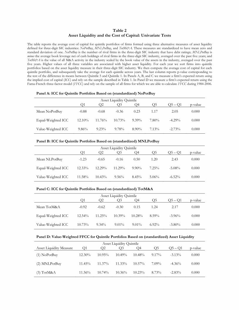
Table 2 Asset Liquidity and the Cost of Capital: Univariate Tests

The table reports the average cost of capital for quintile portfolios of firms formed using three alternative measures of asset liquidity defined for three-digit SIC industries: NoPotBuy, MNLPotBuy, and TotM&A. These measures are standardized to have mean zero and standard deviation of one. NoPotBuy is the number of rival firms in the three-digit SIC industry that have debt ratings; MNLPotBuy is minus the average book leverage net of cash holdings of rival firms in the three-digit SIC industry, averaged over the past five years; and TotM&A is the value of all M&A activity in the industry scaled by the book value of the assets in the industry, averaged over the past five years. Higher values of all three variables are associated with higher asset liquidity. For each year we sort firms into quintile portfolios based on the asset liquidity measure in their three-digit SIC industry. We then compute the average cost of capital for each quintile portfolio, and subsequently take the average for each quintile across years. The last column reports p-value corresponding to the test of the difference in means between Quintile 5 and Quintile 1. In Panels A, B, and C we measure a firm’s expected return using the implied cost of capital (ICC) and rely on the sample described in Table 1. In Panel D we measure a firm’s expected return using the Fama-French three-factor model (FFCC) and rely on the sample of all firms for which we are able to calculate FFCC during 1984-2006.

Panel A: ICC for Quintile Portfolios Based on (standardized) NoPotBuy

Asset Liquidity Quintile Q1 Q2 Q3 Q4 Q5 Q5 – Q1 p-value

Mean NoPotBuy -0.88 -0.68 -0.36 0.23 1.17 2.05 0.000 Equal-Weighted ICC 12.10% 11.76% 10.73% 9.39% 7.80% -4.29% 0.000 Value-Weighted ICC 9.86% 9.23% 9.78% 8.90% 7.13% -2.73% 0.000

Panel B: ICC for Quintile Portfolios Based on (standardized) MNLPotBuy

Asset Liquidity Quintile Q1 Q2 Q3 Q4 Q5 Q5 – Q1 p-value

Mean NLPotBuy -1.23 -0.65 -0.16 0.50 1.20 2.43 0.000 Equal-Weighted ICC 12.33% 12.29% 11.29% 9.90% 7.25% -5.08% 0.000 Value-Weighted ICC 11.58% 10.43% 9.56% 8.45% 5.06% -6.52% 0.000

Panel C: ICC for Quintile Portfolios Based on (standardized) TotM&A

Asset Liquidity Quintile Q1 Q2 Q3 Q4 Q5 Q5 – Q1 p-value

Mean TotM&A -0.92 -0.62 -0.30 0.15 1.24 2.17 0.000 Equal-Weighted ICC 12.54% 11.25% 10.39% 10.28% 8.59% -3.96% 0.000 Value-Weighted ICC 10.73% 9.34% 9.01% 9.01% 6.92% -3.80% 0.000

Panel D: Value-Weighted FFCC for Quintile Portfolios Based on (standardized) Asset Liquidity

Asset Liquidity Quintile Asset Liquidity Measure Q1 Q2 Q3 Q4 Q5 Q5 – Q1 p-value

(1) NoPotBuy 12.30% 10.95% 10.49% 10.48% 9.17% -3.13% 0.000 (2) MNLPotBuy 11.45% 11.37% 11.33% 10.57% 7.09% -4.36% 0.000 (3) TotM&A 11.56% 10.74% 10.36% 10.23% 8.73% -2.83% 0.000

Table 3 Business-Cycle Effects on the Asset-Liquidity Discount

The table reports the results of OLS time-series univariate regressions of the annual average asset-liquidity discount on various business-cycle indicators that we obtain from the St. Louis Federal Reserve Economic Database (FRED). In Panel A we measure a firm’s expected return using the implied cost of capital (ICC) and in Panel B we measure it using the Fama-French three-factor model (FFCC). For the tests using both ICC and FFCC, we calculate three different versions of the asset-liquidity discount using three alternative measures of asset liquidity defined for three-digit SIC industries which are standardized to have mean zero and standard deviation of one. In all cases the asset-liquidity discount is the difference between the average cost of capital (in %) for firms in the highest and lowest asset-liquidity quintiles. The first asset-liquidity discount is calculated using standardized NoPotBuy, which is the number of rival firms in the industry that have debt ratings. The second asset-liquidity discount is calculated using standardized MNLPBuy, which is minus the average book leverage net of cash holdings of rival firms in the three-digit SIC industry, averaged over the past five years. The third asset-liquidity discount is calculated using standardized TotM&A, which is defined as the value of all M&A activity in the industry scaled by the book value of the assets in the industry, averaged over the past five years. Higher values of all three variables are associated with higher asset liquidity. The regressions with the asset liquidity discount based on NoPotBuy are based on the 22 annual observations during the period 1985-2006 and the regressions with asset liquidity discounts based on MNLPotBuy and TotM&A are based on the 23 annual observations during the period 1984-2006 and. GDP Growth is the year-over-year growth in the fourth quarter’s GDP; Capacity Utilization is the utilization rate of the installed capacity in the manufacturing sector for the fourth quarter of each year; Inflation is the year-over-year change in the December’s Consumer Price Index; T-Bill Rate is the average three-month Treasury Bill Rate during the corresponding year; Default Spread is the average spread between the yield on Moody’s Baa corporate bond index and the yield of ten-year government bonds during the year; Market Return is the annual return on the market portfolio (in %). The estimates of the intercept are omitted. The absolute values of t-statistics (in parentheses) are calculated using standard errors obtained from a Newey-West procedure that accounts for any significant autocorrelation. The R2 of each univariate regression is reported in brackets. *, **, and *** indicate statistical significance at 10%, 5%, and 1% levels, respectively.

Panel A: Discount in the ICC

The Dep. Var. is the Asset-Liquidity Discount Based on:

NoPotBuy MNLPotBuy TotM&A

(1) GDP Growth Coef. 0.876*** 0.845*** 0.750*** t-stat (2.86) (6.50) (5.50) R2 [19.88%] [26.27%] [16.27%]

(2) Capacity Utilization Coef. 0.230*** 0.299** 0.463*** t-stat (4.14) (2.60) (5.45) R2 [10.33%] [17.61%] [33.11%]

(3) Inflation Coef. 0.656*** 0.450* 0.972*** t-stat (3.42) (1.81) (4.12) R2 [9.80%] [4.78%] [17.51%]

(4) T-Bill Rate Coef. 0.748*** 0.728*** 0.935*** t-stat (3.67) (7.33) (8.85) R2 [37.32%] [45.68%] [59.20%]

(5) Default Spread Coef. -0.748 -1.802** -2.789*** t-stat (0.75) (2.08) (4.39) R2 [1.95%] [11.67%] [21.95%]

(6) Market Return Coef. 0.038*** 0.049*** 0.045*** t-stat (3.10) (4.87) (3.66) R2 [6.25%] [10.67%] [7.06%]

Panel B: Discount in the FFCC

The Dep. Var. is the Asset-Liquidity Discount Based on:

NoPotBuy MNLPotBuy TotM&A

(1) GDP Growth Coef. 0.845** 0.455*** 0.550*** t-stat (2.30) (4.66) (5.53) R2 23.15% 13.41% 17.37%

(2) Capacity Utilization Coef. 0.483*** 0.140** 0.234*** t-stat (4.00) (2.58) (5.64) R2 56.93% 6.78% 16.72%

(3) Inflation Coef. 0.474* 0.884*** 0.398 t-stat (1.85) (6.18) (1.32) R2 6.40% 32.40% 5.82%

(4) T-Bill Rate Coef. 0.525*** 0.391*** 0.333*** t-stat (3.56) (3.05) (4.41) R2 23.00% 23.11% 14.91%

(5) Default Spread Coef. -3.570*** -1.120*** -1.544*** t-stat (5.91) (4.45) (4.50) R2 55.62% 7.92% 13.34%

Table 4

Asset Liquidity and the Cost of Capital: Multivariate Analysis The table reports the results from regressions of the implied cost of capital (ICC) and the Fama-French three-factor model cost of capital (FFCC) on the three alternative standardized measures of asset liquidity calculated for three-digit SIC industries (NoPotBuy, MNLPotBuy, and TotM&A,) and a set of control variables. Panel A reports the results using ICC. In columns (1), (3), and (5) we report an OLS purely cross-sectional regression using the time-series averages of the variables over the sample period for each firm, with standard errors clustered by three-digit SIC industry. In columns (2), (4), and (6) we report a pooled (panel) OLS regression with three-digit SIC industry fixed effects and year fixed effects, and standard errors clustered by three-digit SIC industry. Panel B reports the results using FFCC. In columns (1), (3), and (5) we report an OLS purely cross-sectional regression using the time-series averages of the variables over the sample period for each firm, with standard errors clustered by three-digit SIC industry. In columns (2), (4), and (6) we report Fama-MacBeth regressions and report t-statistics which are adjusted for autocorrelation using the Newey-West procedure based on 6 lags. The following measures of asset liquidity are standardized to have mean zero and standard deviation of one: NoPotBuy is the number of rival firms in the three-digit SIC industry that have debt ratings; MNLPotBuy is minus the average book leverage net of cash holdings of rival firms in the three-digit SIC industry, averaged over the past five years; and TotM&A is the value of all M&A activity in the industry scaled by the book value of the assets in the industry, averaged over the past five years. Higher values of all three variables are associated with higher asset liquidity. The control variables are as follows: LogAssets is the logarithm of total assets; M/B is the market-to-book assets ratio; DRP is a firm’s percentile ranking based on the yearly distribution of default risk; Blev is book leverage; ROE is return on equity; VolRoe is the standard deviation of ROE over the past five years; FA/TA is fixed assets scaled by total assets; R&DExp is R&D expenditures scaled by sales; LogAge is the logarithm of one plus the number of years since the company was first listed in CRSP; DivPay equals one if the firm pays dividends and zero otherwise; SalGrow is the annual change in the logarithm of sales; LogInvPrice is the logarithm of one divided by the stock price as of the estimation date of ICC; and RetPM is the stock return over the past month. The estimates of the intercept, the year fixed effects, and the industry fixed effects are omitted. The absolute values of the t-statistics are reported in parentheses below each estimate. *, **, and *** indicate statistical significance at 10%, 5%, and 1% levels, respectively.

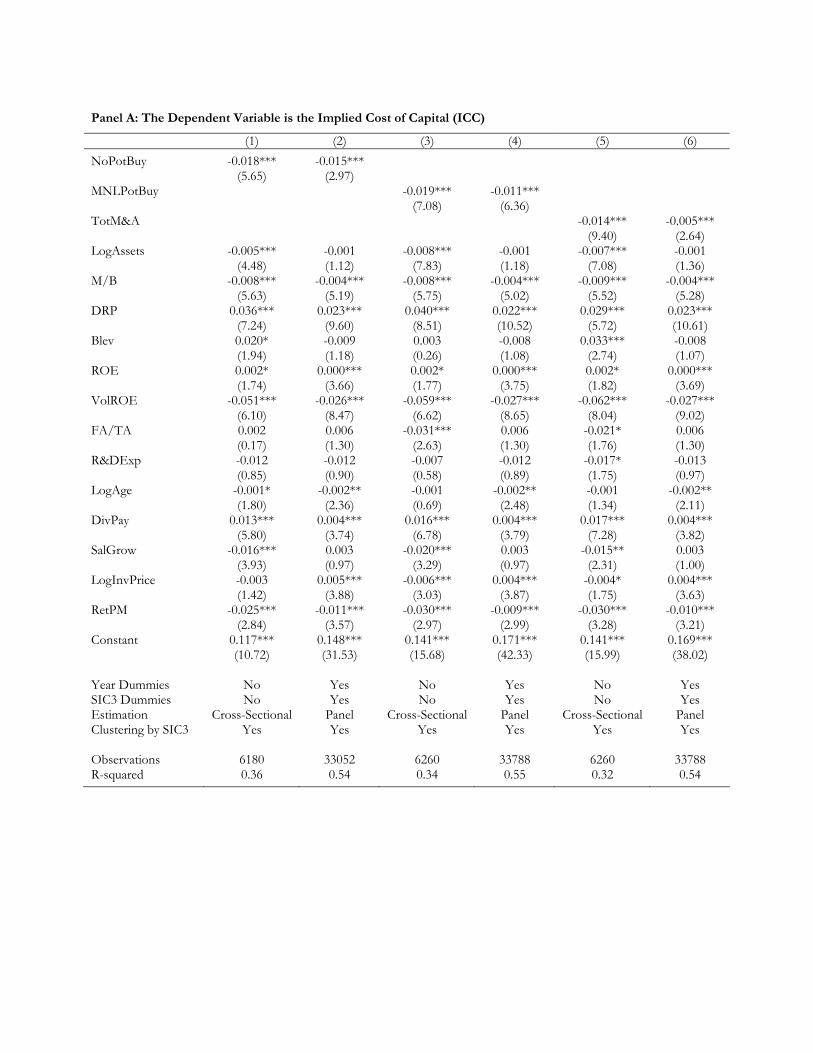
Panel A: The Dependent Variable is the Implied Cost of Capital (ICC)

(1) (2) (3) (4) (5) (6)

NoPotBuy -0.018*** -0.015*** (5.65) (2.97) MNLPotBuy -0.019*** -0.011*** (7.08) (6.36) TotM&A -0.014*** -0.005*** (9.40) (2.64) LogAssets -0.005*** -0.001 -0.008*** -0.001 -0.007*** -0.001 (4.48) (1.12) (7.83) (1.18) (7.08) (1.36) M/B -0.008*** -0.004*** -0.008*** -0.004*** -0.009*** -0.004*** (5.63) (5.19) (5.75) (5.02) (5.52) (5.28) DRP 0.036*** 0.023*** 0.040*** 0.022*** 0.029*** 0.023*** (7.24) (9.60) (8.51) (10.52) (5.72) (10.61) Blev 0.020* -0.009 0.003 -0.008 0.033*** -0.008 (1.94) (1.18) (0.26) (1.08) (2.74) (1.07) ROE 0.002* 0.000*** 0.002* 0.000*** 0.002* 0.000*** (1.74) (3.66) (1.77) (3.75) (1.82) (3.69) VolROE -0.051*** -0.026*** -0.059*** -0.027*** -0.062*** -0.027*** (6.10) (8.47) (6.62) (8.65) (8.04) (9.02) FA/TA 0.002 0.006 -0.031*** 0.006 -0.021* 0.006 (0.17) (1.30) (2.63) (1.30) (1.76) (1.30) R&DExp -0.012 -0.012 -0.007 -0.012 -0.017* -0.013 (0.85) (0.90) (0.58) (0.89) (1.75) (0.97) LogAge -0.001* -0.002** -0.001 -0.002** -0.001 -0.002** (1.80) (2.36) (0.69) (2.48) (1.34) (2.11) DivPay 0.013*** 0.004*** 0.016*** 0.004*** 0.017*** 0.004*** (5.80) (3.74) (6.78) (3.79) (7.28) (3.82) SalGrow -0.016*** 0.003 -0.020*** 0.003 -0.015** 0.003 (3.93) (0.97) (3.29) (0.97) (2.31) (1.00) LogInvPrice -0.003 0.005*** -0.006*** 0.004*** -0.004* 0.004*** (1.42) (3.88) (3.03) (3.87) (1.75) (3.63) RetPM -0.025*** -0.011*** -0.030*** -0.009*** -0.030*** -0.010*** (2.84) (3.57) (2.97) (2.99) (3.28) (3.21) Constant 0.117*** 0.148*** 0.141*** 0.171*** 0.141*** 0.169*** (10.72) (31.53) (15.68) (42.33) (15.99) (38.02) Year Dummies No Yes No Yes No Yes SIC3 Dummies No Yes No Yes No Yes Estimation Cross-Sectional Panel Cross-Sectional Panel Cross-Sectional Panel Clustering by SIC3 Yes Yes Yes Yes Yes Yes Observations 6180 33052 6260 33788 6260 33788 R-squared 0.36 0.54 0.34 0.55 0.32 0.54

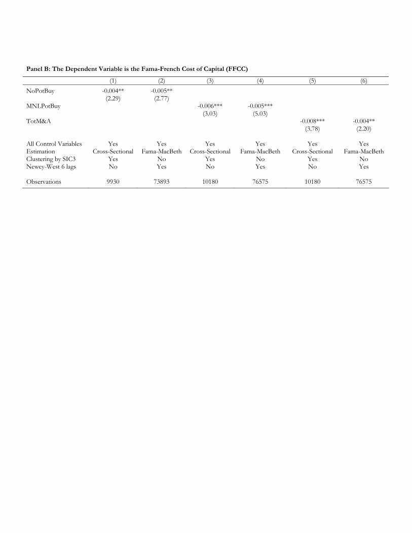
Panel B: The Dependent Variable is the Fama-French Cost of Capital (FFCC)

(1) (2) (3) (4) (5) (6)

NoPotBuy -0.004** -0.005** (2.29) (2.77) MNLPotBuy -0.006*** -0.005*** (3.03) (5.03) TotM&A -0.008*** -0.004** (3.78) (2.20) All Control Variables Yes Yes Yes Yes Yes Yes Estimation Cross-Sectional Fama-MacBeth Cross-Sectional Fama-MacBeth Cross-Sectional Fama-MacBeth Clustering by SIC3 Yes No Yes No Yes No Newey-West 6 lags No Yes No Yes No Yes Observations 9930 73893 10180 76575 10180 76575

Table 5

Inside Vs. Outside Asset Liquidity and the Implied Cost of Capital The table reports the results from regressions of the implied cost of capital (ICC) on two standardized measures of asset liquidity defined at the three-digit SIC industry level (InsM&Q and OutM&A) and a set of control variables. In columns (1) and (3) we report an OLS purely cross-sectional regression using the time-series averages of the variables over the sample period for each firm, with standard errors clustered by three-digit SIC industry. In columns (2) and (4) we report a pooled (panel) OLS regression with three-digit SIC industry fixed effects and year fixed effects, and standard errors clustered by three-digit SIC industry. The following measures of asset liquidity are standardized to have mean zero and standard deviation of one: InsM&A is the value of M&A activity in the industry involving acquirers that operate within the industry scaled by the book value of the assets in the industry, averaged over the past five years; OutM&A is the value of M&A activity in the industry involving acquirers that operate outside the industry scaled by the book value of the assets in the industry, averaged over the past five years. Higher values of all three variables are associated with higher asset liquidity. We also include but do not report the coefficients of the following control variables defined in Table 1: LogAssets, M/B, DRP, Blev, ROE, VolRoe, FA/TA, R&DExp, LogAge, DivPay, SalGrow, LogInvPrice, and RetPM. The estimates of the intercept, the year fixed effects, and the industry fixed effects are also omitted. The absolute values of the t-statistics are reported in parentheses below each estimate. *, **, and *** indicate statistical significance at 10%, 5%, and 1% levels, respectively.

(1) (2) (3) (4)

InsM&A -0.016*** -0.006*** (9.09) (2.78) OutM&A -0.007*** -0.002 (2.80) (1.51) All Control Variables Yes Yes Yes Yes Year Dummies No Yes No Yes SIC3 Dummies No Yes No Yes Estimation Cross-Sectional Panel Cross-Sectional Panel Clustering by SIC3 Yes Yes Yes Yes Observations 6260 33788 6260 33788 R-squared 0.33 0.55 0.29 0.54

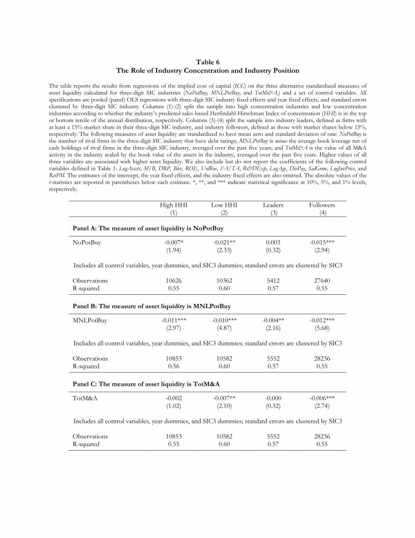
Table 6

The Role of Industry Concentration and Industry Position The table reports the results from regressions of the implied cost of capital (ICC) on the three alternative standardized measures of asset liquidity calculated for three-digit SIC industries (NoPotBuy, MNLPotBuy, and TotM&A,) and a set of control variables. All specifications are pooled (panel) OLS regressions with three-digit SIC industry fixed effects and year fixed effects, and standard errors clustered by three-digit SIC industry. Columns (1)-(2) split the sample into high concentration industries and low concentration industries according to whether the industry’s predicted sales-based Herfindahl-Hirschman Index of concentration (HHI) is in the top or bottom tercile of the annual distribution, respectively. Columns (3)-(4) split the sample into industry leaders, defined as firms with at least a 15% market share in their three-digit SIC industry, and industry followers, defined as those with market shares below 15%, respectively. The following measures of asset liquidity are standardized to have mean zero and standard deviation of one: NoPotBuy is the number of rival firms in the three-digit SIC industry that have debt ratings; MNLPotBuy is minus the average book leverage net of cash holdings of rival firms in the three-digit SIC industry, averaged over the past five years; and TotM&A is the value of all M&A activity in the industry scaled by the book value of the assets in the industry, averaged over the past five years. Higher values of all three variables are associated with higher asset liquidity. We also include but do not report the coefficients of the following control variables defined in Table 1: LogAssets, M/B, DRP, Blev, ROE, VolRoe, FA/TA, R&DExp, LogAge, DivPay, SalGrow, LogInvPrice, and RetPM. The estimates of the intercept, the year fixed effects, and the industry fixed effects are also omitted. The absolute values of the t-statistics are reported in parentheses below each estimate. *, **, and *** indicate statistical significance at 10%, 5%, and 1% levels, respectively.

High HHI Low HHI Leaders Followers (1) (2) (3) (4) Panel A: The measure of asset liquidity is NoPotBuy

NoPotBuy -0.007* -0.021** 0.003 -0.015*** (1.94) (2.33) (0.32) (2.94) Includes all control variables, year dummies, and SIC3 dummies; standard errors are clustered by SIC3 Observations 10626 10362 5412 27640 R-squared 0.55 0.60 0.57 0.55

Panel B: The measure of asset liquidity is MNLPotBuy

MNLPotBuy -0.011*** -0.010*** -0.004** -0.012*** (2.97) (4.87) (2.16) (5.68) Includes all control variables, year dummies, and SIC3 dummies; standard errors are clustered by SIC3 Observations 10853 10582 5552 28236 R-squared 0.56 0.60 0.57 0.55

Panel C: The measure of asset liquidity is TotM&A

TotM&A -0.002 -0.007** -0.000 -0.006*** (1.02) (2.10) (0.32) (2.74) Includes all control variables, year dummies, and SIC3 dummies; standard errors are clustered by SIC3 Observations 10853 10582 5552 28236 R-squared 0.55 0.60 0.57 0.55

Table 7 The Effect of Access to Debt Financing and Default Risk

The table reports the results from regressions of the implied cost of capital (ICC) on the three alternative standardized measures of asset liquidity calculated for three-digit SIC industries (NoPotBuy, MNLPotBuy, and TotM&A,) and a set of control variables. All specifications are pooled (panel) OLS regressions with three-digit SIC industry fixed effects and year fixed effects, and standard errors clustered by three-digit SIC industry. Columns (1)-(2) split the sample into firms with debt but no debt ratings and those whose debt is rated, respectively. Columns (3)-(4) split the sample into firms with high distress risk and low distress risk based on whether the distance of a firm’s probability of default from the industry median is in the top or bottom tercile of the annual distribution across all firms, respectively. The following measures of asset liquidity are standardized to have mean zero and standard deviation of one: NoPotBuy is the number of rival firms in the three-digit SIC industry that have debt ratings; MNLPotBuy is minus the average book leverage net of cash holdings of rival firms in the three-digit SIC industry, averaged over the past five years; and TotM&A is the value of all M&A activity in the industry scaled by the book value of the assets in the industry, averaged over the past five years. Higher values of all three variables are associated with higher asset liquidity. We also include but do not report the coefficients of the following control variables defined in Table 1: LogAssets, M/B, DRP, Blev, ROE, VolRoe, FA/TA, R&DExp, LogAge, DivPay, SalGrow, LogInvPrice, and RetPM. The estimates of the intercept, the year fixed effects, and the industry fixed effects are also omitted. The absolute values of the t-statistics are reported in parentheses below each estimate. *, **, and *** indicate statistical significance at 10%, 5%, and 1% levels, respectively.

Unrated Debt Rated Debt High Default Risk Low Default Risk (1) (2) (3) (4) Panel A: The measure of asset liquidity is NoPotBuy

NoPotBuy -0.014** -0.013*** -0.014*** -0.008*** (2.55) (3.65) (2.78) (2.75)

Includes all control variables, year dummies, and SIC3 dummies; standard errors are clustered by SIC3 Observations 15400 12331 11250 10968 R-squared 0.54 0.54 0.49 0.55

Panel B: The measure of asset liquidity is MNLPotBuy

MNLPotBuy -0.010*** -0.011*** -0.014** -0.009*** (5.65) (3.90) (5.65) (2.94)

Includes all control variables, year dummies, and SIC3 dummies; standard errors are clustered by SIC3 Observations 16079 12331 11501 11211 R-squared 0.55 0.54 0.49 0.56

Panel C: The measure of asset liquidity is TotM&A

TotM&A -0.005** -0.003** -0.007*** -0.002 (2.27) (2.11) (3.44) (1.34)

Includes all control variables, year dummies, and SIC3 dummies; standard errors are clustered by SIC3 Observations 16079 12331 11501 11211 R-squared 0.55 0.53 0.49 0.56

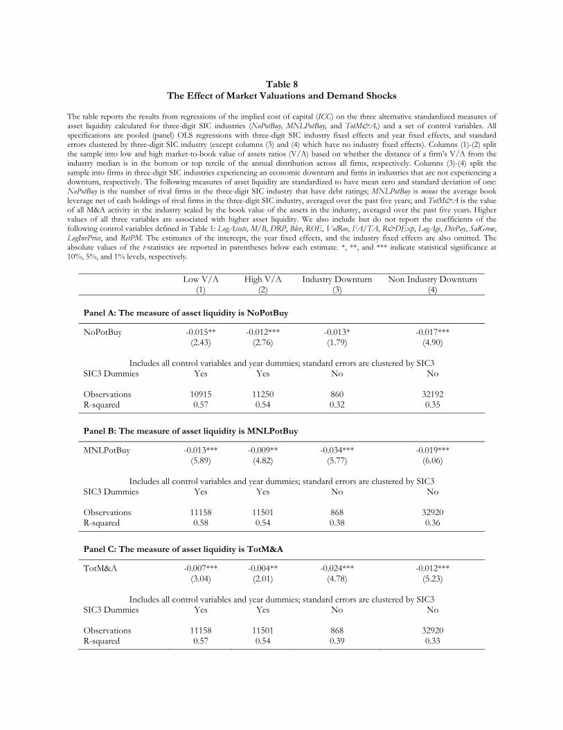
Table 8

The Effect of Market Valuations and Demand Shocks The table reports the results from regressions of the implied cost of capital (ICC) on the three alternative standardized measures of asset liquidity calculated for three-digit SIC industries (NoPotBuy, MNLPotBuy, and TotM&A,) and a set of control variables. All specifications are pooled (panel) OLS regressions with three-digit SIC industry fixed effects and year fixed effects, and standard errors clustered by three-digit SIC industry (except columns (3) and (4) which have no industry fixed effects). Columns (1)-(2) split the sample into low and high market-to-book value of assets ratios (V/A) based on whether the distance of a firm’s V/A from the industry median is in the bottom or top tercile of the annual distribution across all firms, respectively. Columns (3)-(4) split the sample into firms in three-digit SIC industries experiencing an economic downturn and firms in industries that are not experiencing a downturn, respectively. The following measures of asset liquidity are standardized to have mean zero and standard deviation of one: NoPotBuy is the number of rival firms in the three-digit SIC industry that have debt ratings; MNLPotBuy is minus the average book leverage net of cash holdings of rival firms in the three-digit SIC industry, averaged over the past five years; and TotM&A is the value of all M&A activity in the industry scaled by the book value of the assets in the industry, averaged over the past five years. Higher values of all three variables are associated with higher asset liquidity. We also include but do not report the coefficients of the following control variables defined in Table 1: LogAssets, M/B, DRP, Blev, ROE, VolRoe, FA/TA, R&DExp, LogAge, DivPay, SalGrow, LogInvPrice, and RetPM. The estimates of the intercept, the year fixed effects, and the industry fixed effects are also omitted. The absolute values of the t-statistics are reported in parentheses below each estimate. *, **, and *** indicate statistical significance at 10%, 5%, and 1% levels, respectively.

Low V/A High V/A Industry Downturn Non Industry Downturn (1) (2) (3) (4) Panel A: The measure of asset liquidity is NoPotBuy

NoPotBuy -0.015** -0.012*** -0.013* -0.017*** (2.43) (2.76) (1.79) (4.90)

Includes all control variables and year dummies; standard errors are clustered by SIC3 SIC3 Dummies Yes Yes No No Observations 10915 11250 860 32192 R-squared 0.57 0.54 0.32 0.35

Panel B: The measure of asset liquidity is MNLPotBuy

MNLPotBuy -0.013*** -0.009** -0.034*** -0.019*** (5.89) (4.82) (5.77) (6.06)

Includes all control variables and year dummies; standard errors are clustered by SIC3 SIC3 Dummies Yes Yes No No Observations 11158 11501 868 32920 R-squared 0.58 0.54 0.38 0.36

Panel C: The measure of asset liquidity is TotM&A

TotM&A -0.007*** -0.004** -0.024*** -0.012*** (3.04) (2.01) (4.78) (5.23)

Includes all control variables and year dummies; standard errors are clustered by SIC3 SIC3 Dummies Yes Yes No No Observations 11158 11501 868 32920 R-squared 0.57 0.54 0.39 0.33

Table 9

Asset Liquidity and the Implied Cost of Capital: Controlling for Industry Valuation The table reports the results from regressions of the implied cost of capital (ICC) on the three alternative standardized measures of asset liquidity calculated for three-digit SIC industries (NoPotBuy, MNLPotBuy, and TotM&A), measures of industry valuation (LogIndMBE) or miss-valuation (IndRelVal) also defined for three-digit SIC industries, and a set of control variables. In columns (1) and (3) we report an OLS purely cross-sectional regression using the time-series averages of the variables over the sample period for each firm, with standard errors clustered by three-digit SIC industry. In columns (2) and (4) we report a pooled (panel) OLS regression with three-digit SIC industry fixed effects and year fixed effects, and standard errors clustered by three-digit SIC industry. The following measures of asset liquidity are standardized to have mean zero and standard deviation of one: NoPotBuy is the number of rival firms in the three-digit SIC industry that have debt ratings; MNLPotBuy is minus the average book leverage net of cash holdings of rival firms in the three-digit SIC industry, averaged over the past five years; and TotM&A is the value of all M&A activity in the industry scaled by the book value of the assets in the industry, averaged over the past five years. Higher values of all three variables are associated with higher asset liquidity. LogIndMBE is the logarithm of the mean market-to-book equity ratio in the firm’s industry and IndRelVal is the industry’s relative valuation, computed as the difference between the industry market-to-book equity ratio and its predicted value based on the benchmark Pastor and Veronesi (2003) specification. We also include but do not report the coefficients of the following control variables defined in Table 1: LogAssets, M/B, DRP, Blev, ROE, VolRoe, FA/TA, R&DExp, LogAge, DivPay, SalGrow, LogInvPrice, and RetPM. The estimates of the intercept, the year fixed effects, and the industry fixed effects are also omitted. The absolute values of the t-statistics are reported in parentheses below each estimate. *, **, and *** indicate statistical significance at 10%, 5%, and 1% levels, respectively.

(1) (2) (3) (4)

All Control Variables Yes Yes Yes Yes Year Dummies No Yes No Yes SIC3 Dummies No Yes No Yes Estimation Cross-Sectional Panel Cross-Sectional Panel Clustering by SIC3 Yes Yes Yes Yes

Panel A: The measure of asset liquidity is NoPotBuy

NoPotBuy -0.014*** -0.015*** -0.018*** -0.015*** (4.51) (2.98) (5.69) (3.00) LogIndMBE -0.024*** 0.002 (5.15) (1.31) IndRelVal 0.006 -0.004 (1.19) (1.36)

Panel B: The measure of asset liquidity is MNLPotBuy

MNLPotBuy -0.013*** -0.011*** -0.019*** -0.011*** (5.78) (6.38) (7.30) (6.70) LogIndMBE -0.025*** 0.003 (6.39) (1.51) IndRelVal 0.016** -0.001 (2.42) (0.41)

Panel C: The measure of asset liquidity is TotM&A

TotM&A -0.011*** -0.005*** -0.014*** -0.005*** (8.81) (2.62) (9.62) (2.65) LogIndMBE -0.031*** 0.002 (9.45) (1.17) IndRelVal 0.004 -0.003 (0.54) (0.96)

Table 10

Asset Liquidity and the Implied Cost of Capital: Industry-Level Tests The table reports the results from industry-level regressions of the implied cost of capital (ICC) on the three alternative standardized measures of asset liquidity calculated for three-digit SIC industries (NoPotBuy, MNLPotBuy, and TotM&A,) and a set of control variables. For this purpose, all firm-level variables are converted into three-digit SIC industry medians for each year. In columns (1), (3), and (5) we report an OLS purely cross-sectional industry-level regression using the time-series averages of the variables over the sample period for each industry, with standard errors clustered by three-digit SIC industry. In columns (2), (4), and (6) we report a pooled (panel) industry-level OLS regression with three-digit SIC industry fixed effects and year fixed effects, and standard errors clustered by three-digit SIC industry. The following measures of asset liquidity are standardized to have mean zero and standard deviation of one: NoPotBuy is the number of rival firms in the three-digit SIC industry that have debt ratings; MNLPotBuy is minus the average book leverage net of cash holdings of rival firms in the three-digit SIC industry, averaged over the past five years; and TotM&A is the value of all M&A activity in the industry scaled by the book value of the assets in the industry, averaged over the past five years. Higher values of all three variables are associated with higher asset liquidity. We also include but do not report the coefficients of the following control variables defined in Table 1: LogAssets, M/B, DRP, Blev, ROE, VolRoe, FA/TA, R&DExp, LogAge, DivPay, SalGrow, LogInvPrice, and RetPM. The estimates of the intercept, the year fixed effects, and the industry fixed effects are also omitted. The absolute values of the t-statistics are reported in parentheses below each estimate. *, **, and *** indicate statistical significance at 10%, 5%, and 1% levels, respectively.

(1) (2) (3) (4) (5) (6)

NoPotBuy -0.012** -0.015** (2.27) (2.33) MNLPotBuy -0.016*** -0.013*** (3.24) (5.78) TotM&A -0.011** -0.003* (2.47) (1.81) All Control Variables Yes Yes Yes Yes Yes Yes Year Dummies No Yes No Yes No Yes SIC3 Dummies No Yes No Yes No Yes Estimation Cross-Sectional Panel Cross-Sectional Panel Cross-Sectional Panel Clustering by SIC3 Yes Yes Yes Yes Yes Yes Observations 303 4631 304 4793 304 4793 R-squared 0.59 0.86 0.58 0.85 0.58 0.85

Table 11 Asset Liquidity and Unlevered Implied Cost of Capital

The table reports the results from regressions of the unlevered implied cost of capital (UNLICC) on the three alternative standardized measures of asset liquidity calculated for three-digit SIC industries (NoPotBuy, MNLPotBuy, and TotM&A) and a set of control variables. In columns (1), (3), and (5) we report an OLS purely cross-sectional regression using the time-series averages of the variables over the sample period for each firm, with standard errors clustered by three-digit SIC industry. In columns (2), (4), and (6) we report a pooled (panel) OLS regression with three-digit SIC industry fixed effects and year fixed effects, and standard errors clustered by three-digit SIC industry. The following measures of asset liquidity are standardized to have mean zero and standard deviation of one: NoPotBuy is the number of rival firms in the three-digit SIC industry that have debt ratings; MNLPotBuy is minus the average book leverage net of cash holdings of rival firms in the three-digit SIC industry, averaged over the past five years; and TotM&A is the value of all M&A activity in the industry scaled by the book value of the assets in the industry, averaged over the past five years. Higher values of all three variables are associated with higher asset liquidity. We also include but do not report the coefficients of the following control variables defined in Table 1: LogAssets, M/B, DRP, ROE, VolRoe, FA/TA, R&DExp, LogAge, DivPay, SalGrow, LogInvPrice, and RetPM. The estimates of the intercept, the year fixed effects, and the industry fixed effects are also omitted. The absolute values of the t-statistics are reported in parentheses below each estimate. *, **, and *** indicate statistical significance at 10%, 5%, and 1% levels, respectively.

(1) (2) (3) (4) (5) (6)

NoPotBuy -0.015*** -0.012** (4.33) (2.49) MNLPotBuy -0.016*** -0.009*** (7.35) (6.29) TotM&A -0.013*** -0.004** (8.52) (2.25) All Control Variables Yes Yes Yes Yes Yes Yes Year Dummies No Yes No Yes No Yes SIC3 Dummies No Yes No Yes No Yes Estimation Cross-Sectional Panel Cross-Sectional Panel Cross-Sectional Panel Clustering by SIC3 Yes Yes Yes Yes Yes Yes Observations 6180 33052 6260 33788 6260 33788 R-squared 0.36 0.56 0.36 0.57 0.34 0.57