Biometrics DOI: 10.1111/biom.12139

Assessing the Significance of Global and Local Correlations underSpatial Autocorrelation: A Nonparametric Approach

Julia Viladomat,1,* Rahul Mazumder,2 Alex McInturff,3 Douglas J. McCauley,4 Trevor Hastie1

1Department of Statistics, Stanford University, Stanford, California 94305, U.S.A.2Department of Statistics, Columbia University, New York, New York 10027, U.S.A.

3Department of Biology, Stanford University, Stanford, California 94305, U.S.A.4Department of Ecology, Evolution, and Marine Biology, UC Santa Barbara, Santa Barbara,

California 93106, U.S.A.∗email: juliaviladomat@gmail.com

Summary. We propose a method to test the correlation of two random fields when they are both spatially autocorrelated. Inthis scenario, the assumption of independence for the pair of observations in the standard test does not hold, and as a resultwe reject in many cases where there is no effect (the precision of the null distribution is overestimated). Our method recoversthe null distribution taking into account the autocorrelation. It uses Monte-Carlo methods, and focuses on permuting, andthen smoothing and scaling one of the variables to destroy the correlation with the other, while maintaining at the same timethe initial autocorrelation. With this simulation model, any test based on the independence of two (or more) random fieldscan be constructed. This research was motivated by a project in biodiversity and conservation in the Biology Department atStanford University.

Key words: Geostatistics; Monte-Carlo methods; Resampling; Spatial autocorrelation; Spatial statistics; Variogram.

1. Motivation

Assessing significance of the correlation coefficient is notstraightforward if the values of the variables involved varysmoothly with location (throughout the article smooth refersto spatial autocorrelation, and it may be the case that thevariable changes abruptly over a short distance). With spa-tially autocorrelated data, nearby points may provide almostidentical information. Hence there is a tension between samplesize, resolution and the number of independent measurements;that is, at some level, more data, meaning sampling the pro-cess at a higher resolution, does not mean more information.As a result, classical tests Fisher (1915) tend to incorrectlyreject the null (larger type II errors). Some work has beendone, particularly in the field of Geostatistics, to overcomethis problem. For instance, Clifford, Richardson, and Hemon(1989) propose a method that estimates an effective samplesize M < N to be used in such tests, in an attempt to capturethe real uncertainty. The correlation coefficient is thus eval-uated with a Student’s t distribution with M degrees of free-dom (distribution with larger variance), which accounts forthe loss of precision due to the underlying spatial component.The method, however, is developed for Gaussian random fieldsand in reality smoothed processes tend to be non-Gaussian.

We propose a Monte-Carlo method to test the correlationof two random fields that takes account of the spatial auto-correlation. By

(1) randomly permuting the values of one of the fieldsacross space we eliminate the dependence betweenthem, and

(2) smoothing and scaling the permuted field we approx-imately recover, with the help of the variogram, thespatial structure suppressed in (1).

In the same spirit, Allard, Brix, and Chadoeuf (2001) pro-pose a method that is based on random local rotations, butapplied to the characteristics of the spatial structure of pointprocesses, where the intensity (rate parameter) is assumed tobe constant at small scales and varies at large scales, the op-posite situation we encounter with random fields, were theautocorrelation usually fades away as the distance increases.

By repeating steps (1) and (2) many times, we can obtainapproximate realizations of the null distribution of interest. Infact, with this simulation model, it is possible to examine thenull distribution of a larger variety of statistics. In particularany test based on the independence of two (or more) randomfields can be constructed, the simplest example being the testfor a single Pearson’s correlation coefficient between the tworandom fields. We will call it global correlation.

Other spatially local tests may be of interest—for exam-ple, which regions show strong correlation between the twofields—the question that our collaborators posed (McCauleyet al., 2012). They mapped the locations of sites over theworld using two criteria:

� amount of species richness—biodiversity, and� travel time in days needed to reach the nearest city—

remoteness.

Figure 1a and b represent both these fields, and we seethat they are spatially very smooth. Are remoteness and

© 2014, The International Biometric Society 1

2 Biometrics

Figure 1. Top right: Biodiversity as a function of domain. Top left: Remoteness as a function of domain. Bottom: Localcorrelations between biodiversity and remoteness using a Gaussian kernel with bandwidth λ = 5.281 (see Appendix 2), wherethe blue circles indicate the extent of the neighborhood for 5 locations at random. The gray areas correspond to areas withno data. (a) Biodiversity. (b) Remoteness. (c) Local correlations.

biodiversity correlated with one another? that is, are theremore species in remote areas that are better insulated fromhuman disturbance? To succinctly communicate the strengthof these correlations, the authors were interested in reportinga p-value map for the areas where overlap between remote-ness and biodiversity occurs. Initially they used Geograph-ically Weighted Regression methods (Fotheringham, Bruns-don, and Charlton, 2002), a set of regression techniques thattackle spatially varying relationships. This book has capturedconsiderable attention in the Geostatistics community. How-ever, these methods focus on comparing coefficients for dif-ferent spatial areas, and identifying the areas with strongerrelationships, but with no assessment to whether the coeffi-cients in the model are significant or not.

Given the map of correlations in Figure 1c, where eachvalue corresponds to the correlation between biodiversity andremoteness in a given neighborhood (we will call them localcorrelations), we will apply our method and produce a mapof p values, where each p-value assesses significance of thecorrelation in that particular location. See Appendix 2 fordetails on how to calculate the local correlations.

We organize the article as follows. In Section 2 we show theresults of applying our method to the biodiversity dataset.Section 3 illustrates the limitations of the standard test un-der spatial autocorrelation. Section 4 describes in detail thealgorithm proposed in this article, and in Section 5 we studythe behavior of the method by performing power and type Ierror analyses, and compares it to the approach in Clifford

Test for the Correlation When the Variables Are Smoothed 3

et al. (1989). We conclude and summarize our findings in thediscussion.

2. Biodiversity Data

Protecting remote ecosystems is the future of global diver-sity, WWF ecologists divided the world into 16 unique regions(Biomes) based on land cover and climate. In this article, andfor simplicity, we will focus on the part of the biodiversitydataset that corresponds to the American region of Biome 1(tropical and subtropical moist broadleaf forests) to illustrateour methodology.

Biodiversity (X) is the result of estimating the number ofspecies of plants, amphibians, birds and mammals in an areaof 100 km × 100 km and centered at location s. The estimatesfor the 4 groups is normalized to a maximum score of 10, withX being the average of those normalized counts. Remoteness(Y) combines a number of data sets that influence speed oftravel: road networks, angle of slope, density of vegetation,river courses, etc. It takes values between 1 and 8 and indi-cates the travel time in days needed to reach the nearest citylarger than 50,000 inhabitants from location s, where 8 rep-resents any travel time larger than 7 days. Our sample is de-noted by (Xs,Ys) = [(Xs1 , Ys1), . . . , (XsN , YsN )], s = (s1 . . . sN),where si ∈ R2 are the longitude and latitude coordinates ofobservation i and N = 19,926.

2.1. The Empirical and Smoothed Variogram forBiodiversity

The theoretical variogram is a function describing the de-gree of spatial dependence of a random field Xs. It is de-fined as the variance of the difference between field valuesat two locations si and sj across realizations of the field:γ(si, sj) = 1

2Var(Xsi − Xsj ), see Cressie (1993). The empirical

variogram for the sample Xs1 , . . . , XsN is the collection of pairsof distances uij = ‖si − sj‖ between si and sj, and their corre-sponding variogram ordinates vij = 1

2(Xsi − Xsj )

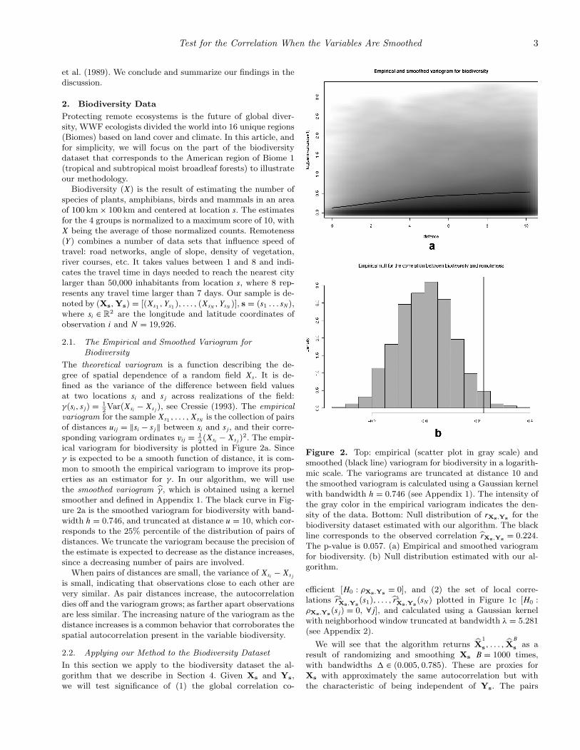
2. The empir-ical variogram for biodiversity is plotted in Figure 2a. Sinceγ is expected to be a smooth function of distance, it is com-mon to smooth the empirical variogram to improve its prop-erties as an estimator for γ. In our algorithm, we will usethe smoothed variogram γ, which is obtained using a kernelsmoother and defined in Appendix 1. The black curve in Fig-ure 2a is the smoothed variogram for biodiversity with band-width h = 0.746, and truncated at distance u = 10, which cor-responds to the 25% percentile of the distribution of pairs ofdistances. We truncate the variogram because the precision ofthe estimate is expected to decrease as the distance increases,since a decreasing number of pairs are involved.

When pairs of distances are small, the variance of Xsi − Xsj

is small, indicating that observations close to each other arevery similar. As pair distances increase, the autocorrelationdies off and the variogram grows; as farther apart observationsare less similar. The increasing nature of the variogram as thedistance increases is a common behavior that corroborates thespatial autocorrelation present in the variable biodiversity.

2.2. Applying our Method to the Biodiversity Dataset

In this section we apply to the biodiversity dataset the al-gorithm that we describe in Section 4. Given Xs and Ys,we will test significance of (1) the global correlation co-

Figure 2. Top: empirical (scatter plot in gray scale) andsmoothed (black line) variogram for biodiversity in a logarith-mic scale. The variograms are truncated at distance 10 andthe smoothed variogram is calculated using a Gaussian kernelwith bandwidth h = 0.746 (see Appendix 1). The intensity ofthe gray color in the empirical variogram indicates the den-sity of the data. Bottom: Null distribution of rXs,Ys for thebiodiversity dataset estimated with our algorithm. The blackline corresponds to the observed correlation rXs,Ys = 0.224.The p-value is 0.057. (a) Empirical and smoothed variogramfor biodiversity. (b) Null distribution estimated with our al-gorithm.

efficient [H0 : ρXs,Ys = 0], and (2) the set of local corre-lations rλ

Xs,Ys(s1), . . . , r

λXs,Ys

(sN) plotted in Figure 1c [H0 :ρXs,Ys(sj) = 0, ∀j], and calculated using a Gaussian kernelwith neighborhood window truncated at bandwidth λ = 5.281(see Appendix 2).

We will see that the algorithm returns X1

s, . . . , XB

s as aresult of randomizing and smoothing Xs B = 1000 times,with bandwidths � ∈ (0.005, 0.785). These are proxies forXs with approximately the same autocorrelation but withthe characteristic of being independent of Ys. The pairs

4 Biometrics

(X1

s,Ys), . . . , (XB

s ,Ys) will be used to test the situations (1)and (2) above.

We chose to randomize Xs (biodiversity), as we are free topick the most convenient one, since the purpose is to breakthe dependence between both variables.

2.2.1. Testing the global correlation. The observed globalcorrelation coefficient between biodiversity and remotenessis rXs,Ys = 0.224. We use r = (r1, . . . , rB) as an estimateof the sampling distribution of rXs,Ys under the null hy-

pothesis of independence, where ri = cor(Xi

s,Ys); see Fig-ure 2b. Using this null distribution to test H0 : ρXs,Ys =0, the p-value is p

r= P(|rXs,Ys | > |rXs,Ys |) = 1

B

∑B

i=1I[|ri| >

|rXs,Ys |] = 0.057 (indicated with a black line in Figure 2b).Had we assumed that the sample pairs were independent, andused instead a Student’s t with N − 2 degrees of freedom, thep-value would have been effectively zero, since the variance ofthe Student’s t distribution is significantly smaller.

2.2.2. Testing local correlations. Each pair of random

fields (Xi

s,Ys), i = 1, . . . , B, can be used to calculate a new

map of local correlations under the null hypothesis (Xi

s

and Ys are constructed to be independent). Hence we cancompute local p values in exactly the same was as wasdone globally above. A sample distribution of the statisticrXs,Ys(sj) under the null is r(sj) = (r1(sj), . . . , rB(sj)), whereri(sj) = rλ

Xi

s,Ys

(sj). The p-value for testing H0 : ρXs,Ys(sj) =0 at location sj is psj = P(|rXs,Ys(sj)| > |rλ

Xs,Ys(sj)|) =

1B

∑B

i=1I[|ri(sj)| > |rλ

Xs,Ys(sj)|]. The resulting p-value map is

plotted in Figure 3, where we can identify the regions thatare strongly correlated. For comparison, we also plot the mapof p values had we used the standard test.

3. Behavior of rXs,Ys Under SpatialAutocorrelation

If (x1, y1), . . . , (xN, yN) is an independent and normally dis-tributed sample, the distribution for the Pearson’s correlationcoefficient under ρX,Y = 0 is

fN(r) = (1 − r2)N−42

B{ 12, 1

2(N − 2)} , ‖r‖ ≤ 1. (1)

The statistic t = (N−2)12 r

(1−r2)12

is used to test for H0 : ρX,Y = 0,

which follows a Student’s t distribution with N − 2 degreesof freedom, see Kenney and Keeping (1951).

In the previous section we have seen that even thoughthe sample size of the biodiversity dataset was very large(N = 19,296), the sample distribution for rXs,Ys was some-what wide (Figure 2b).

This emphasizes the following point, which we demonstratevia a simulation. For a pair of spatially correlated randomfields, the sample size or, more precisely, the resolution atwhich the fields are sampled, can play less of a role in thebehavior of the distribution of rXs,Ys ; rather it is the extentof the spatial autocorrelation that determines this distribution(see Walther, 1997 for an equivalent problem with time series).

Figure 3. Top: map of p values for the correlations betweenbiodiversity and remoteness in Figure 1c, obtained with ourmethod with B = 1000 and � ∈ (0.005, 0.785). Bottom: p val-ues map if we assume that there is no spatial autocorrelationand use the standard test to assess the local correlations.

Let Ws be a stationary and isotropic Gaussian randomfield, s ∈ R2, with Matern autocorrelation function ϕ(u) =[2κ−1�(κ)]−1(u/φ)κKκ(u/φ) where φ > 0 is the scale, and theshape parameter κ > 0 determines the smoothness of the pro-cess, var(Ws) = σ2. For κ = 0.5, the Matern autocorrelationfunction reduces to the exponential, and when κ → ∞ to theGaussian.

Suppose Xsi is generated by a stationary process

Xsi = Wsi + Zi (2)

with Zi being mutually independent and identically dis-tributed with zero mean and nugget variance τ2 (measure-ment error), see Diggle and Ribeiro (2007). The theoreticalvariogram of Xsi under stationarity is described in Appendix1 and illustrated in Web Figure 4.

Test for the Correlation When the Variables Are Smoothed 5

Figure 4. Top, left and right: Illustration of Xs and Ys, two independent realizations of a Gaussian random field withexponential autocorrelation function with φ = 0.03 and grid size g = 0.01. Bottom, left and right: null distribution for rXs,Ys

returned by the algorithm (blue), for a Gaussian and exponential autocorrelation function respectively, together with the truenull (pink) obtained by simulating from model (2). The corresponding 95% Confidence Intervals are added to the plot. (a)Gaussian random field Xs. (b) Random field Ys, independent of Xs. (c) Gaussian autocorrelation function. (d) Exponentialautocorrelation function.

Figure 4a and b are Xs and Ys, two independent real-izations of this process in the grid [0, 1] × [0, 1] with reso-lution N = 101 × 101 = 10,201, and parameters κ = 0.5 andφ = 0.30. We have used the R package RandomFields to sim-ulate these processes (R Core Team, 2013; Schlather et al.,2013).

In Web Figure 1, Web Figure 1a is the scatter plot of Xs

and Ys, whereas Web Figure 1d is the scatter plot of two inde-pendent samples, each of them mutually independent (non-spatially correlated) and normally distributed. The correla-tion coefficient is much larger for Xs and Ys (rXs,Ys = 0.3).

Web Figure 1b and c are two new sets of independent sim-ulated processes Xs and Ys, showing negative strong corre-lation and a correlation closer to zero respectively. Thus, aswe have seen, a consequence of the spatial autocorrelation isa larger variance for the distribution of rXs,Ys . In fact, thelarger κ, the larger the variance. Intuitively, consider the ex-treme case of two very smooth one-dimensional fields (i.e.,lines) with randomly chosen orientations (slopes); the corre-lation of sampled pairs will either be −1 and +1 dependingon the randomly chosen orientation; a maximal variance situ-ation. The same intuition applies to higher-dimensional fields.

6 Biometrics

The null distribution for rXs,Ys under ρXs,Ys = 0 can be es-timated by generating the independent pairs (Xi

s,Yis). With

this distribution, the probability of observing values as ex-treme or more than 0.3 is 0.16, with no evidence against H0.

Although Xs and Ys have been constructed to be indepen-dent of each other, if we use the Student’s t distribution totest H0 : ρXs,Ys = 0, the p-value for rXs,Ys = 0.3 is 0.

4. The Algorithm

We propose a method that approximately recovers the nulldistribution of rXs,Ys , or any other statistic based on the in-dependence of Xs and Ys. The following scheme summarizesthe main steps of the algorithm.

Let Xs and Ys be a realization of two random fields. Repeatthe following two steps B times:

(1) Randomly permute the values of Xs over s, which wedenote by Xπ(s); this means Xπ(s) and Ys are indepen-dent.

(2) Smooth and scale Xπ(s) to produce Xs, such that itssmoothed variogram γ approximately matches γ(Xs);

that is, the transformed variable Xs has approximatelythe same autocorrelation structure as Xs.

The random fields X1

s, . . . , XB

s have approximately thesame autocorrelation structure as Xs, but are each indepen-

dent of Ys. Hence, the pairs (X1

s,Ys), . . . , (XB

s ,Ys) are theingredients for the calculation of a null distribution. For in-stance, the distribution of rXs,Ys under H0 : ρXs,Ys = 0 can

be approximated by r = (r1, . . . , rB), where ri = cor(Xi

s,Ys),but we could proceed equivalently with any other statisticbased on the independence of Xs and Ys.

Note that we do not pose restrictions on which random fieldto permute, but the algorithm assumes that Xs is stationary.

Step 4 of the algorithm is described in detail in the followingsection.

4.1. Step 2: Matching Variograms

This step focuses on recovering the intrinsic spatial structureof Xs that was eliminated with the random permutation. Aswe have seen, the null distribution of rXs,Ys is mainly deter-mined by the amount of autocorrelation, and this step willdetermine how well we are able to recover it. Our approachis non-parametric, which implies that the variogram match-ing does not rely on model assumptions, such as choosing aparametric model for the variogram.

Formally, the problem reduces to choosing a variogramfrom the family

β γ(Xδs) + α, (3)

that best approximates γ(Xs), the smoothed variogram of Xs.Let Xπ(s) be the permuted random field obtained in step 4

above. Choose � to be a set of values for the proportion ofneighbors to consider for the smoothing step.

(1) Calculate the smoothed variogram γ(Xs) by smoothingthe empirical variogram of Xs (see Appendix 1).

(2) For each δ ∈ � repeat:(a) Construct the smoothed variable Xδ

s using a ker-nel smoother that fits a constant regression toXπ(s) at each location sj (see Appendix 2).

(b) Calculate γ(Xδs) as in 4.1.

(c) Fit a linear regression between γ(Xδs) and γ(Xs),

where (αδ, βδ) are the least-squares estimates.(3) Choose δ∗ ∈ � such that the sum of squares of the resid-

uals of the fit in 4.1 is minimized.

(4) Transform Xδ∗s by X

δ∗

s = |βδ∗ | 12 Xδ∗

s + |αδ∗ | 12 Z, where Z

is a vector of mutually independent and identically dis-tributed Zi’s with zero mean and unit variance.

By varying the tuning parameter or proportion of neighborsδ in step 4.1 we obtain a family of variograms with differentshapes, choosing the one more similar to the variogram of theoriginal variable Xs.

The linear transformation in step 4.1 ensures that the

scale and intercept of γ(Xδ∗

s ) match those of γ(Xs), sincethe smoothing in step 4.1 has changed the scale of Xs (thesmoother Xδ∗

s , the smaller the variance), in addition to theintercept (nugget variance) of γ(Xs).

The variogram of the random field Xδ∗

s is a member of the

family in (3), and Xδ∗

s has been constructed to match γ(Xs)in shape, scale, and intercept.

Note that |βδ∗ |var(Xδ∗s ) is an estimate of σ2 in (A.2),

|αδ∗ | is an estimate of τ2, and correspondingly var(Xδ∗

s ) =|βδ∗ |var(Xδ∗

s ) + |αδ∗ | is an estimate of σ2 + τ2.For an illustration of the variogram matching see Figure 5.

Different δs result in different shapes for γ(Xδ

s), and the best

match between γ(Xs) and γ(Xδ

s) (gray) is reached with δ =0.085. The residual sum of squares of linearly regressing γ(Xδ

s)on γ(Xs) for different values of δ are plotted in Web Figure 2.

5. Simulation Results

In this section we study the performance of our method fortesting H0 : ρXs,Ys = 0 by comparing the estimate of the nulldistribution for rXs,Ys provided by our algorithm with an es-timate of the true null distribution.

In addition to that, we carry out power and type I erroranalyses (Section 5.2), and compare the results to Clifford’sapproach.

Let Xs and Ys be two independent Gaussian randomfields in the grid [0, 1] × [0, 1] with resolution N = 101 × 101 =10, 201, following model (2) with σ2 = 1, μ = 0, and:

(1) Gaussian autocorrelation function ϕ(u) = exp[−(u/φ)2]with scale parameter φ = 0.3.

(2) Exponential autocorrelation function ϕ(u)= exp(−u/φ)with φ = 0.3.

We apply our algorithm to one realization of the pair (Xs,Ys)in situations 5 and 5, with B = 1000 and bandwidths �gauss =(0.1, 0.2, . . . , 0.9) and �exp = (0.07, 0.080, . . . , 0.18), respec-tively.

Test for the Correlation When the Variables Are Smoothed 7

Figure 5. Variogram matching between the original biodiversity variable Xs (black) and the transformed variable Xδ

s (gray)for four different values of bandwidth: � = (0.020, 0.045, 0.085, 0.120). The best match is reached with δ = 0.085.

The null distributions that the algorithm returns are plot-ted respectively in Figure 4c and d, together with the truenulls obtained by simulating 1000 times the pairs (Xi

s,Yis)

from the models above. The results are slightly better for 5,but we manage to recover the null in both situations.

5.1. Clifford’s Effective Sample Size

We briefly review Clifford’s procedure prior to using it as acomparator. Clifford et al. (1989) propose to use fM(r) in (1)as the distribution of reference under the null. The varianceof fM(r) is 1

M−1. Their suggestion is to estimate the effective

sample size M by M =⌊1 + 1

σ2r

⌋, as a result of equating 1

M−1to

σ2r , the variance of the sample correlation. Hence, an estimate

for the null distribution of rXs,Ys is fM

(r).

How to Estimate σ2r . In Clifford et al. (1989)’s appendix

they prove that σ2r = var(SXsYs )

E(S2Xs

)E(S2Ys

)to the first order, and un-

der the assumption of normality, where SXsYs is the sam-ple covariance, S2

Xsand S2

Ysare the sample variances of Xs

and Ys, var(SXsYs) = trace(�ξs�ηs), �ξs = P�XsP , �ηs

=P�YsP , �Xs , and �Ys are the covariance matrices of Xs

and Ys respectively, P = I − 1N11′ and 1 is a vector of 1’s of

dimension N.An estimate for var(SXsYs) is obtained by imposing a strat-

ified structure on �Xs and �Ys . More precisely, they as-sume that the set of all ordered pairs of elements of s canbe divided into strata S0, S1, S2, . . ., and that the covariances

within strata are constant. Then, σ2r =

∑kNkCXs (k)CYs (k)

N2S2Xs

S2Ys

,

where Nk is the number of pairs in stratum Sk and CXs(k) =1Nk

∑(i,j)∈Sk

(Xsi − Xk)(Xsj − Xk) is an autocovariance estimatefor stratum Sk. They use the sample variogram to choose thenumber of strata.

5.2. Power Analysis and Type I Error Estimates

In this section we estimate the power and type I error of thetest for our procedure, and compare it to Clifford’s approach.

Web Figure 3 summarizes different scenarios for the nulland alternative distributions, as a function of the effect ρ wewould like to detect and the amount of spatial autocorrelationφ. The power to detect a fixed effect ρ decreases as the spatialautocorrelation increases. Equivalently, for a fixed φ the powerdecreases with the effect size. These data have been simulatedassuming we know the truth, and indicates how well we cando in each situation. The grid size g is set to 0.05 (N = 441),but identical results were obtained for grid size g = 0.01 (N =10, 201).

The simulation experiment goes as follows. For each combi-nation of autocorrelation in φ ∈ (0.05, 0.1, 0.3) and resolutionin g ∈ (0.05, 0.01), and for the power calculations, for each sizeeffect in ρ ∈ (0.2, 0.5, 0.8), we simulate 10 independent pairs(Xj

s,Yjs) from the usual model in the grid [0, 1] × [0, 1], with

grid size g and Gaussian autocorrelation function with scaleparameter φ. Then we do the following:

(1) Apply our algorithm to each pair (Xjs,Y

js) with B =

1000, �φ=0.3 = (0.1, 0.2, . . . , 0.9), �φ=0.1 = (0.03, 0.034,

. . . , 0.074), and �φ=0.05 = (0.013, 0.014, . . . , 0.027) re-spectively. Let (r1, . . . , r10) be the resulting 10 nulls.

(2) Apply Clifford’s method to each pair (Xjs,Y

js) by

generating B independent and normally distributedrandom vectors Xi and Y i of dimension M. Let(rCl

1 , . . . , rCl10) be the resulting 10 nulls, where rCl

j =(rCl

1j , . . . , rClBj ) and rCl

ij = cor(Xi, Y i).

In addition to that, (rTr1 , . . . , rTr

10) are 10 nulls under thetruth, by simulating B independent pairs (Xi

s,Yis) from the

same model, where rTrj = (rCl

1j , . . . , rTrBj ) and rTr

ij = cor(Xis,Y

is).

8 Biometrics

Table 1Type I error estimates obtained by contrasting pairs simulated under H0 : ρXs,Ys = 0, to the null distribution returned by our

algorithm and Clifford’s method, in addition to the true null obtained by simulating independent pairs under model (2)

Type I error estimates

φ = 0.05 φ = 0.1 φ = 0.3

Grid size = 0.05 0.052 (0.024) 0.046 (0.022) 0.048 (0.024) True0.059 (0.029) 0.056 (0.035) 0.051 (0.041) Ours0.055 (0.027) 0.055 (0.029) 0.093 (0.045) Clifford

Grid size = 0.01 0.053 (0.027) 0.049 (0.023) 0.051 (0.022) True0.075 (0.030) 0.051 (0.027) 0.050 (0.045) Ours0.055 (0.027) 0.058 (0.026) 0.086 (0.044) Clifford

Results are presented for different levels of autocorrelation and resolution: φ ∈ (0.05, 0.1, 0.3) and g ∈ (0.05, 0.01). The standard errorsare in brackets.

The type I error of the test should be equal to thesignificance level α = 0.05. We use the nulls (rTr

1 , . . . , rTr10),

(r1, . . . , r10) and (rCl1 , . . . , rCl

10) to estimate the type I errorsassociated to both methods and the truth. We draw 100 sam-ples from (Xk

s,Yks) under H0 : ρXs,Ys = 0, and use respec-

tively rTrj , rj and rCl

j to assess significance of rk = cor(Xks,Y

ks),

for k = 1, . . . , 100. Out of the 100 samples, the proportion oftimes the p values are smaller than α = 0.05 is an estimateof the type I error. We repeat the same process for 100 repli-cates, obtaining 100 type I error estimates. We then repeatthe process again for each null j = 1, . . . , 10 and average the10 × 100 type I error estimates, which are shown in Table 1.Estimates of the standard errors are obtained by computing

the standard deviation of the 10 × 100 estimates, and appearin brackets in the table.

The power of the test is calculated using a similar sam-pling scheme. We generate pairs (Xk

s,Yks) as before, but then

transform Yks ← ηXk

s + Yks with η = ρ/

√(1 − ρ2) (leading to

a population correlation of ρ). The rk’s are thus obtained un-der the alternative hypotheses H1 : ρXs,Ys = ρ. We then fol-low the same procedure as was done for the type-I errors,namely steps (1) and (2) above, leading to the power esti-mates in Table 2.

We highlight the values in Table 1 that most deviate fromα. Type I error estimates for our method are close to α, whichis less of a case for Clifford’s method, except for φ = 0.05.

Table 2Power estimates obtained by contrasting pairs simulated under H1 : ρXs,Ys = ρ, to the null distribution returned by ouralgorithm and Clifford’s method, in addition to the true null obtained by simulating correlated pairs under model (2)

Power estimates

φ = 0.05 φ = 0.1 φ = 0.3

Grid size = 0.05ρ = 0.2 0.921 (0.026) 0.418 (0.059) 0.103 (0.034) True

0.926 (0.031) 0.444 (0.087) 0.089 (0.042) Ours0.926 (0.030) 0.446 (0.077) 0.153 (0.045) Clifford

ρ = 0.5 1 (0) 0.997 (0.005) 0.426 (0.055) True1 (0) 0.997 (0.005) 0.420 (0.089) Ours1 (0) 0.997 (0.005) 0.558 (0.100) Clifford

ρ = 0.8 1 (0) 1 (0) 0.951 (0.021) True1 (0) 1 (0) 0.879 (0.127) Ours1 (0) 1 (0) 0.950 (0.045) Clifford

Grid size = 0.01ρ = 0.2 0.915 (0.033) 0.405 (0.052) 0.104 (0.030) True

0.935 (0.031) 0.404 (0.073) 0.124 (0.069) Ours0.927 (0.030) 0.415 (0.064) 0.169 (0.046) Clifford

ρ = 0.5 1 (0) 0.996 (0.007) 0.424 (0.059) True1 (0) 0.996 (0.007) 0.391 (0.154) Ours1 (0) 0.996 (0.007) 0.510 (0.111) Clifford

ρ = 0.8 1 (0) 1 (0) 0.937 (0.022) True1 (0) 1 (0) 0.949 (0.030) Ours1 (0) 1 (0) 0.972 (0.018) Clifford

Results are presented for different levels of autocorrelation, effect size and resolution: φ ∈ (0.05, 0.1, 0.3), ρ ∈ (0.2, 0.5, 0.8), and g ∈(0.05, 0.01).

Test for the Correlation When the Variables Are Smoothed 9

Note also in Table 2 that power results for our methodare typically closer to the power obtained under the truth,and that better power results in Clifford’s case go along withlarger type I error estimates, these values are highlighted inthe table.

Finally, observe that there are no obvious differences be-tween both resolutions, where the grid sizes g = 0.01 andg = 0.05 correspond to N = 101 × 101 = 10,201 and N = 21 ×21 = 441, respectively. This is important, as it highlights thefact that the power of the analysis is mainly driven by theautocorrelation, and even if we increase significantly the res-olution, the power stays the same as it is constrained by φ.

6. Discussion

This articles addresses the consequences of spatial autocorre-lation on the distribution of statistics like correlation betweenrandom fields. We develop a nonparametric approach for sam-pling from the null-hypothesis of independence, that involvesthree steps:

(1) pick one of the fields and estimate the spatial autocor-relation structure via its variogram

(2) randomly permute the values in this field(3) apply a local smoothing to the permuted values, using a

bandwidth and rescaling so that its resulting variogrammatches the original in step (1).

Steps (2) and (3) are repeated B times to obtain B realizationsfrom the null. These realizations can be used to measure manydifferent kinds of independence, including measures of localdependence.

A referee of an earlier draft of this article made a usefulsuggestion for an alternative and more direct approach. Theirsuggestion was to simulate a Gaussian random field accord-ing to a model of the variogram, with parameters estimatedby weighted least square, maximum likelihood or compositelikelihood, with non-Gaussian data transformed to normalscores prior to the estimation of the variogram. One of theadvantages of our method, though, is that it does not relyon model assumptions, which turns it into a more flexible,non-parametric approach.

Allard et al. (2001) address a related problem in the con-text of pairs of point processes, where the focus is on localcorrelations between pairs of realizations of counts. They ran-domize one of the processes using local rotations, under theassumption that locally the process rates are constant. Ourrandomization scheme treats broader range correlations, sothe locally constant assumption is not appropriate.

Another approach is proposed by Clifford et al. (1989),where they estimate an effective sample size that takes theautocorrelation into account. We compare this approach toour method through simulations, which show that our algo-rithm behaves well in practice, with type I error estimatesclose to α, and power estimates close to the maximum powerfor each combination of φ and ρ.

Since correlation may exist simultaneously at a number ofdifferent geographical scales, the method can be used to cal-culate a p-value for the global correlation, as well as p valuesfor the local correlations (p values map), summarizing the

strength of the relationship between both fields in a particu-lar location.

One of the important consequences of autocorrelation isthat increasing the sample size does not necessarily increasethe power to find significance. There is no concept of samplesize, since what we observe is one realization of the randomfield, and the amount of data that we have is the resolution.The information that the sample provides is limited by thespatial autocorrelation. Consequently, in practice it may bemore important to focus on using methods that adjust forautocorrelation, than on collecting more data.

7. Supplementary Materials

Web Figures referenced in Sections 3, 4.1, 5.2, and Appendix1 are available with this article at the Biometrics website onWiley Online Library.

The prototype R code is now available online athttp://www.stanford.edu/ hastie/Papers/biodiversity/

viladomat code.R and at the Biometrics website in WileyOnline Library.

Acknowledgements

We thank Paul Switzer for some suggestions early on in thisproject. Trevor Hastie and Rahul Mazumder were partiallysupported by grant DMS-1007719 from the National ScienceFoundation (NSF), and grant RO1-EB001988-15 from the Na-tional Institutes of Health. Douglas McCauley was supportedby NSF grants DEB-0909670 and GRFP-2006040852 as wellfunding from the Wood’s Institute for the environment. JuliaViladomat was supported by the Spanish Ministry of Edu-cation through the program “Programa Nacional de Movili-dad de Recursos Humanos del Plan Nacional de I-D+i 2008–2011.”

Appendix A

The smoothed variogram γ for Xs is defined by smoothingthe empirical variogram using a kernel smoother:

γ(u0) =∑N

i=1

∑N

j=i+1wijvij∑N

i=1

∑N

j=i+1wij

. (A.1)

It assigns weights that die off smoothly as distance tou0 increases, with wij = Kh(‖u0 − uij‖), uij = ‖si − sj‖, vij =12(Xsi − Xsj )

2 and Kh(x) = exp {−(2.68x)2

2h2}, the Gaussian ker-

nel is scaled so that their quartiles are at ±0.25h, with h

being the bandwidth (R function ksmooth). The variogram γ

is obtained by evaluating (A.1) at distances u = (u1, . . . , u100)uniformly chosen within the range of pair distances uij.

The theoretical variogram of a stationary random fieldXsi = Wsi + Zi in (2) is:

γ(u) = σ2{1 − ϕ(u)} + τ2, (A.2)

where ϕ(u) is the autocorrelation function of Wsi , typically amonotone decreasing function with ϕ(0) = 1 and ϕ(u) → 0 asu → ∞. Its most important feature is its behavior near u = 0,and how quickly it approaches zero when u increases, which

10 Biometrics

reflects the physical extent of the spatial autocorrelation inthe process. When ϕ(u) = 0 for u greater than some finitevalue, this value is known as the range of the variogram. Theintercept τ2 corresponds to the nugget variance, the condi-tional variance of each measured value Xsi given the under-lying signal value Wsi . The sill is the asymptote τ2 + σ2 andcorresponds to the variance of the observation process Xsi .Web Figure 4 gives a schematic illustration.

Appendix B

We smooth a given random field Xs by fitting a local con-stant regression at locations s1, . . . , sN using the R packagelocfit (Loader, 2013):

fδ(s) =∑

‖s−si‖≤λswsiXsi∑

‖s−si‖≤λswsi

, (B.1)

where wsi = Kλs(‖s − si‖), Kλs

(x) = exp(

−2.5x2

2λ2s

)is a Gaussian

kernel, and λs controls the smoothness of the fit. For a fittingpoint s, λs is such that the neighborhood contains the k = �Nδ�nearest points to s in Euclidean distance, where δ ∈ (0, 1) isa tuning parameter that indicates the proportion of neigh-bors. Each fδ(s) is estimated with the k observations that fallwithin the ball Bλs

(s) centered at s and of radius λs (the ker-nel truncates at one standard deviation). We use a varying λs

because it reduces data sparsity problems by increasing theradius in regions with fewer observations.

The smoothed variable Xδs in Section 4.1 in step 4.1 of the

algorithm is the result of fitting the function (B.1) to Xπ(s).The local correlations in Figure 1c are calculated using this

same approach. The local correlation at location s is definedas:

r λXs,Ys

(s) =∑

‖s−si‖≤λwsi(Xsi − Xs)(Ysi − Ys)√∑

‖s−si‖≤λwsi(Xsi − Xs)2

∑‖s−si‖≤λ

wsi(Ysi − Ys)2,

(B.2)

where Xs =∑

wsiXsi∑

wsi

and Ys =∑

wsiYsi∑

wsi

. We then compute

(B.2) by breaking it down and separately evaluating the quan-

tities∑

wsiXsi ,∑

wsiYsi ,∑

wsiXsiYsi ,∑

wsiX2si

and∑

wsiY2si

using locfit as above.

References

Allard, D., Brix, A., and Chadoeuf, J. (2001). Testing local in-dependence between two point processes. Biometrics 57,508–517.

Clifford, P., Richardson, S., and Hemon, D. (1989). Assessing thesignificance of the correlation between two spatial processes.Biometrics 45, 123–134.

Cressie, N. A. (1993). Statistics for Spatial Data. New York (Cressiebook): John Wiley.

Diggle, P. J. and Ribeiro, P. J. (2007). Model-Based Geostatistics.New York (Diggle book): Springer.

Fisher, R. A. (1915). Frequency distribution of the values of thecorrelation coefficient in samples from an indefinitely largepopulation. Biometrika 10, 507–521.

Fotheringham, A. S., Brunsdon, C., and Charlton, M. (2002). Ge-ographically Weighted Regression: The Analysis of SpatiallyVarying Relationships. Chichester, England; Hoboken, NJ(Fotheringham book): John Wiley.

Kenney, J. F. and Keeping, E. S. (1951). Mathematics of Statistics(Part Two). New York: D. Van Nostrand Company, Inc.

Loader, C. (2013). Locfit: Local Regression, Likelihood and DensityEstimation. R package version 1.5-9.1.

McCauley, D. J., McInturff, A., Nunez, T. A., Young, H. S., Vilado-mat, J., Mazumder, R., et al. (2012). Nature’s last stand:Identifying the world’s most remote and biodiverse ecosys-tems, In review.

R Core Team (2013). R: A Language and Environment for Statisti-cal Computing. Vienna, Austria: R Foundation for StatisticalComputing.

Schlather, M., Menck, P., Singleton, R., Pfaff, B., and Team, R. C.(2013). RandomFields: Simulation and Analysis of RandomFields. R package version 2.0.66.

Walther, G. (1997). Absence of correlation between the solar neu-trino flux and the sunspot number. Physical Review Letters79, 4522–4524.

Received January 2013. Revised December 2013.Accepted December 2013.