Assessing significance in a Markov chainwithout mixingMaria Chikinaa, Alan Friezeb, and Wesley Pegdenb,1

aDepartment of Computational and Systems Biology, University of Pittsburgh, Pittsburgh, PA 15213; and bDepartment of Mathematical Sciences, CarnegieMellon University, Pittsburgh, PA 15213

Edited by Kenneth W. Wachter, University of California, Berkeley, CA, and approved January 24, 2017 (received for review October 21, 2016)

We present a statistical test to detect that a presented state ofa reversible Markov chain was not chosen from a stationary dis-tribution. In particular, given a value function for the states ofthe Markov chain, we would like to show rigorously that the pre-sented state is an outlier with respect to the values, by establish-ing a p value under the null hypothesis that it was chosen froma stationary distribution of the chain. A simple heuristic used inpractice is to sample ranks of states from long random trajecto-ries on the Markov chain and compare these with the rank of thepresented state; if the presented state is a 0.1% outlier comparedwith the sampled ranks (its rank is in the bottom 0.1% of sam-pled ranks), then this observation should correspond to a p valueof 0.001. This significance is not rigorous, however, without goodbounds on the mixing time of the Markov chain. Our test is thefollowing: Given the presented state in the Markov chain, take arandom walk from the presented state for any number of steps.We prove that observing that the presented state is an ε-outlieron the walk is significant at p =

√2ε under the null hypoth-

esis that the state was chosen from a stationary distribution.We assume nothing about the Markov chain beyond reversibil-ity and show that significance at p≈

√ε is best possible in gen-

eral. We illustrate the use of our test with a potential applica-tion to the rigorous detection of gerrymandering in Congressionaldistricting.

Markov chain | mixing time | gerrymandering | outlier | p value

The essential problem in statistics is to bound the probabil-ity of a surprising observation under a null hypothesis that

observations are being drawn from some unbiased probabilitydistribution. This calculation can fail to be straightforward fora number of reasons. On the one hand, defining the way inwhich the outcome is surprising requires care; for example, intri-cate techniques have been developed to allow sophisticated anal-ysis of cases where multiple hypotheses are being tested. Onthe other hand, the correct choice of the unbiased distributionimplied by the null hypothesis is often not immediately clear;classical tools like the t test are often applied by making sim-plifying assumptions about the distribution in such cases. If thedistribution is well-defined but is not be amenable to mathemat-ical analysis, a p value can still be calculated using bootstrappingif test samples can be drawn from the distribution.

A third way for p value calculations to be nontrivial occurswhen the observation is surprising in a simple way and the nullhypothesis distribution is known but where there is no simplealgorithm to draw samples from this distribution. In these cases,the best candidate method to sample from the null hypothesis isoften through a Markov chain, which essentially takes a long ran-dom walk on the possible values of the distribution. Under suit-able conditions, theorems are available that guarantee that thechain converges to its stationary distribution, allowing a randomsample to be drawn from a distribution quantifiably close to thetarget distribution. This principle has given rise to diverse appli-cations of Markov chains, including to simulations of chemicalreactions, Markov chain Monte Carlo statistical methods, pro-tein folding, and statistical physics models.

A persistent problem in applications of Markov chains is theoften unknown rate at which the chain converges with the sta-tionary distribution (1, 2). It is rare to have rigorous results onthe mixing time of a real-world Markov chain, which means that,in practice, sampling is performed by running a Markov chainfor a “long time” and hoping that sufficient mixing has occurred.In some applications, such as in simulations of the Potts modelfrom statistical physics, practitioners have developed modifiedMarkov chains in the hopes of achieving faster convergence (3),but such algorithms have still been shown to have exponentialmixing times in many settings (4–6).

In this article, we are concerned with the problem of assess-ing statistical significance in a Markov chain without requiringresults on the mixing time of the chain or indeed, any specialstructure at all in the chain beyond reversibility. Formally, weconsider a reversible Markov chainM on a state space Σ, whichhas an associated label function ω : Σ→<. (The definition ofMarkov chain is recalled at the end of this section.) The labelsconstitute auxiliary information and are not assumed to have anyrelationship to the transition probabilities ofM. We would liketo show that a presented state σ0 is unusual for states drawn froma stationary distribution π. If we have good bounds on the mix-ing time ofM, then we can simply sample from a distribution ofω(π) and use bootstrapping to obtain a rigorous p value for thesignificance of the smallness of the label of σ0. However, suchbounds are rarely available.

We propose the following simple and rigorous test to detectthat σ0 is unusual relative to states chosen randomly accordingto π, which does not require bounds on the mixing rate ofM.

The√ε test. Observe a trajectory σ0, σ1, σ2 . . . , σk from the

state σ0 for any fixed k . The event that ω(σ0) is an ε-outlieramong ω(σ0), . . . , ω(σk ) is significant at p =

√2ε under the null

hypothesis that σ0∼π.Here, we say that a real number α0 is an ε-outlier among

α0, α2, . . . , αk if there are, at most, ε(k + 1) indices i for which

Significance

Markov chains are simple mathematical objects that can beused to generate random samples from a probability spaceby taking a random walk on elements of the space. Unfortu-nately, in applications, it is often unknown how long a chainmust be run to generate good samples, and in practice, thetime required is often simply too long. This difficulty can pre-clude the possibility of using Markov chains to make rigorousstatistical claims in many cases. We develop a rigorous sta-tistical test for Markov chains which can avoid this problem,and apply it to the problem of detecting bias in Congressionaldistricting.

Author contributions: M.C., A.F., and W.P. performed research and wrote the paper.

The authors declare no conflict of interest.

This article is a PNAS Direct Submission.1To whom correspondence should be addressed. Email: wes@math.cmu.edu.

This article contains supporting information online at www.pnas.org/lookup/suppl/doi:10.1073/pnas.1617540114/-/DCSupplemental.

2860–2864 | PNAS | March 14, 2017 | vol. 114 | no. 11 www.pnas.org/cgi/doi/10.1073/pnas.1617540114

MA

THEM

ATI

CSPO

LITI

CAL

SCIE

NCE

S

αi ≤α0. In particular, note for the√ε test that the only relevant

feature of the label function is the ranking that it imposes on theelements of Σ. In SI Text, we consider the statistical power ofthe test and show that the relationship p≈

√ε is best possible.

We leave as an open question whether the constant√

2 can beimproved.

Roughly speaking, this kind of test is possible, because areversible Markov chain cannot have many local outliers (Fig. 1).Rigorously, the validity of the test is a consequence of the follow-ing theorem.

Theorem 1.1. Let M=X0,X1, . . . be a reversible Markovchain with a stationary distribution π, and suppose the states ofM have real-valued labels. If X0∼π, then for any fixed k , theprobability that the label of X0 is an ε-outlier from among thelist of labels observed in the trajectory X0,X1,X2, . . . ,Xk is, atmost,

√2ε.

We emphasize that Theorem 1.1 makes no assumptions on thestructure of the Markov chain beyond reversibility. In particular,it applies even if the chain is not irreducible (in other words, evenif the state space is not connected), although in this case, thechain will never mix.

In Detecting Bias in Political Districting, we apply the testto Markov chains generating random political districting forwhich no results on rapid mixing exist. In particular, we showthat, for various simple choices of constraints on what con-stitutes a “valid” Congressional districting (e.g., that the dis-tricts are contiguous and satisfy certain geometric constraints),the current Congressional districting of Pennsylvania is signifi-cantly biased under the null hypothesis of a districting chosenat random from the set of valid districting. (We obtain p valuesbetween ≈ 2.5 ·10−4 and ≈ 8.1 ·10−7 for the constraints that weconsidered.)

One hypothetical application of the√ε test is the possibility of

rigorously showing that a chain is not mixed. In particular, sup-pose that Research Group 1 has run a reversible Markov chain

Fig. 1. This schematic illustrates a region of a potentially much largerMarkov chain with a very simple structure; from each state seen here, ajump is made with equal probability to each of four neighboring states. Col-ors from green to pink represent labels from small to large, respectively. Itis impossible to know from this local region alone whether the highlightedgreen state has unusually small label in this chain overall. However, to anunusual degree, this state is a local outlier. The

√ε test is based on the fact

that no reversible Markov chain can have too many local outliers.

for n1 steps and believes that this was sufficient to mix the chain.Research Group 2 runs the chain for another n2 steps, producinga trajectory of total length n1 +n2, and notices that a property ofinterest changes in these n2 additional steps. Heuristically, thisobservation suggests that n1 steps were not sufficient to mix thechain, and the

√ε test quantifies this reasoning rigorously. For

this application, however, we must allow X0 to be distributed notexactly as the stationary distribution π but as some distributionπ′ with total variation distance to π that is small, as is the sce-nario for a “mixed” Markov chain. In SI Text, we give a versionof Theorem 1.1, which applies in this scenario.

One area of research related to this manuscript concernsmethods for perfect sampling from Markov chains. Beginningwith the Coupling from the Past (CFTP) algorithm of Propp andWilson (7, 8) and several extensions (9, 10), these techniques aredesigned to allow sampling of states exactly from the station-ary distribution π without having rigorous bounds on the mix-ing time of the chain. Compared with the

√ε test, perfect sam-

pling techniques have the disadvantages that they require theMarkov chain to possess a certain structure for the method to beimplementable and that the time that it takes to generate eachperfect sample is unbounded. Moreover, although perfect sam-pling methods do not require rigorous bounds on mixing timesto work, they will not run efficiently on a slowly mixing chain.The point is that for a chain that has the right structure and thatactually mixes quickly (despite an absence of a rigorous boundon the mixing time), algorithms like CFTP can be used to rig-orously generate perfect samples. However, the

√ε test applies

to any reversible Markov chain, regardless of the structure, andhas running time k chosen by the user. Importantly, it is quitepossible that the test can detect bias in a sample even when k ismuch smaller than the mixing time of the chain, which seems tobe the case in the districting example discussed in Detecting Biasin Political Districting. Of course, unlike perfect sampling meth-ods, the

√ε test can only be used to show that a given sample is

not chosen from π; it does not give a way for generating samplesfrom π.

DefinitionsWe remind the reader that a Markov chain is a discrete time ran-dom process; at each step, the chain jumps to a new state, whichonly depends on the previous state. Formally, a Markov chainMon a state space Σ is a sequenceM=X0,X1,X2, . . . of randomvariables taking values in Σ (which correspond to states that maybe occupied at each step), such that, for any σ, σ0, . . . , σn−1 ∈ Σ,

Pr(Xn = σ|X0 = σ0,X1 = σ1, . . . ,Xn−1 = σn−1)

= Pr(X1 = σ|X0 = σn−1).

Note that a Markov chain is completely described by the distribu-tion of X0 and the transition probabilities Pr(X1 =σ1|X0 =σ0)for all pairs σ0, σ1 ∈ Σ. Terminology is often abused, so that theMarkov chain refers only to the ensemble of transition probabil-ities, regardless of the choice of distribution for X0.

With this abuse of terminology, a stationary distribution forthe Markov chain is a distribution π, such that X0∼π impliesthat X1∼π and therefore, that Xi ∼π for all i . When the dis-tribution of X0 is a stationary distribution, the Markov chainX0,X1, . . . is said to be stationary. A stationary chain is saidto be reversible if, for all i , k , the sequence of random variables(Xi ,Xi+1, . . . ,Xi+k ) is identical in distribution to the sequence(Xi+k ,Xi+k−1, . . . ,Xi). Finally, a chain is reducible if there is apair of states σ0, σ1, such that σ1 is inaccessible from σ0 via legaltransitions and irreducible otherwise.

A simple example of a Markov chain is a random walk on adirected graph beginning from an initial vertex X0 chosen fromsome distribution. Here, Σ is the vertex set of the directed graph.If we are allowed to label the directed edges with positive reals

Chikina et al. PNAS | March 14, 2017 | vol. 114 | no. 11 | 2861

and if the probability of traveling along an arc is proportionalto the label of the arc (among those leaving the present vertex),then any Markov chain has such a representation, because thetransition probability Pr(X1 =σ1|X0 =σ0) can be taken as thelabel of the arc from σ0 to σ1. Finally, if the graph is undirected,the corresponding Markov chain is reversible.

Detecting Bias in Political DistrictingA central feature of American democracy is the selection of Con-gressional districts in which local elections are held to directlyelect national representatives. Because a separate election is heldin each district, the proportions of party affiliations of the slateof representatives elected in a state do not always match the pro-portions of statewide votes cast for each party. In practice, largedeviations from this seemingly desirable target do occur.

Various tests have been proposed to detect “gerrymandering”of districting, in which a district is drawn in such a way as to biasthe resulting slate of representatives toward one party, which canbe accomplished by concentrating voters of the unfavored partyin a few districts. One class of methods to detect gerrymanderingconcerns heuristic “smell tests,” which judge whether districtingseems generally reasonable in its statistical properties (11, 12).For example, such tests may frown on districting in which differ-ence between the mean and median votes on district by districtbasis is unusually large (13).

The simplest statistical smell test, of course, is whether theparty affiliation of the elected slate of representatives is close inproportion to the party affiliations of votes for representatives.Many states have failed this simple test spectacularly, such as inPennsylvania; in 2012, 48.77% of votes were cast for Republicanrepresentatives and 50.20% of votes were cast for Democrat rep-resentatives in an election that resulted in a slate of 13 Republi-can representatives and 5 Democrat representatives.

Heuristic statistical tests such as these all suffer from lack ofrigor, however, because of the fact that the statistical proper-ties of “typical” districting are not rigorously characterized. Forexample, it has been shown (14) that Democrats may be at a nat-ural disadvantage when drawing electoral maps, even when nobias is at play, because Democrat voters are often highly geo-graphically concentrated in urban areas. Particularly problematicis that the degree of geographic clustering of partisans is highlyvariable from state to state: what looks like gerrymandered dis-tricting in one state may be a natural consequence of geographyin another.

Some work has been done in which the properties of valid dis-tricting are defined (which may be required to have roughly equalpopulations among districts, districts with reasonable bound-aries, etc.), so that the characteristics of a given districting canbe compared with what would be typical for valid districting ofthe state in question, by using computers to generate randomdistricting (15, 16); there is discussion of this in ref. 13. However,much of this work has relied on heuristic sampling procedures,

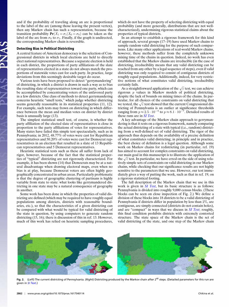
Fig. 2. (Left) The current districting of Pennsylvania. (Right) Districting produced by the Markov chain after 240 steps. (Detailed parameters for this run aregiven in SI Text.)

which do not have the property of selecting districting with equalprobability (and more generally, distributions that are not well-characterized), undermining rigorous statistical claims about theproperties of typical districts.

In an attempt to establish a rigorous framework for this kindof approach, several groups (17–19) have used Markov chains tosample random valid districting for the purpose of such compar-isons. Like many other applications of real-world Markov chains,however, these methods suffer from the completely unknownmixing time of the chains in question. Indeed, no work has evenestablished that the Markov chains are irreducible (in the case ofdistricting, irreducibility means that any valid districting can bereached from any other by a legal sequence of steps), even if validdistricting was only required to consist of contiguous districts ofroughly equal populations. Additionally, indeed, for very restric-tive notions of what constitutes valid districting, irreducibilitycertainly fails.

As a straightforward application of the√ε test, we can achieve

rigorous p values in Markov models of political districting,despite the lack of bounds on mixing times of the chains. In par-ticular, for all choices of the constraints on valid districting thatwe tested, the

√ε test showed that the current Congressional dis-

tricting of Pennsylvania is an outlier at significance thresholdsranging from p≈ 2.5 · 10−4 to p≈ 8.1 · 10−7. Detailed results ofthese runs are in SI Text.

A key advantage of the Markov chain approach to gerryman-dering is that it rests on a rigorous framework, namely comparingthe actual districting of a state with typical (i.e., random) district-ing from a well-defined set of valid districting. The rigor of theapproach thus depends on the availability of a precise definitionof what constitutes valid districting; in principle and in practice,the best choice of definition is a legal question. Although somework on Markov chains for redistricting (in particular, ref. 19)has aimed to account for complex constraints on valid districting,our main goal in this manuscript is to illustrate the application ofthe√ε test. In particular, we have erred on the side of using rela-

tively simple sets of constraints on valid districting in our Markovchains, while checking that our significance results are not highlysensitive to the parameters that we use. However, our test imme-diately gives a way of putting the work, such as that in ref. 19, ona rigorous statistical footing.

The full description of the Markov chain that we use in thiswork is given in SI Text, but its basic structure is as follows:Pennsylvania is divided into roughly 9,000 census blocks. (Theseblocks can be seen on close inspection of Fig. 2.) We define adivision of these blocks into 18 districts to be a valid districting ofPennsylvania if districts differ in population by less than 2%, arecontiguous, are simply connected (districts do not contain holes),and are “compact” in ways that we discuss in SI Text; roughly,this final condition prohibits districts with extremely contortedstructure. The state space of the Markov chain is the set ofvalid districting of the state, and one step of the Markov chain

2862 | www.pnas.org/cgi/doi/10.1073/pnas.1617540114 Chikina et al.

MA

THEM

ATI

CSPO

LITI

CAL

SCIE

NCE

S

consists of randomly swapping a precinct on the boundary of adistrict to a neighboring district if the result is still a valid dis-tricting. As we discuss in SI Text, the chain is adjusted slightly toensure that the uniform distribution on valid districting is indeeda stationary distribution for the chain. Observe that this Markovchain has a potentially huge state space; if the only constraint onvalid districting was that the districts have roughly equal popu-lation, there would be 1010000 or so valid districtings. Althoughcontiguity and especially, compactness are severe restrictionsthat will decrease this number substantially, it seems difficultto compute effective upper bounds on the number of result-ing valid districtings, and certainly, it is still enormous. Impres-sively, these considerations are all immaterial to our very generalmethod.

Applying the√ε test involves the choice of a label function

ω(σ), which assigns a real number to each districting. We haveconducted runs using two label functions: ωvar is the (negative)variance of the proportion of Democrats in each district of thedistricting (as measured by 2012 presidential votes), and ωMMis the difference between the median and mean of the propor-tions of Democrats in each district; ωMM is motivated by thefact that this metric has a long history of use in gerrymanderingand is directly tied to the goals of gerrymandering, whereas theuse of the variance is motivated by the fact that it can changequickly with small changes in districtings. These two choicesare discussed further in SI Text, but an important point is thatour use of these label functions is not based on an assumptionthat small values of ωvar or ωMM directly imply gerrymandering.Instead, because Theorem 1.1 is valid for any fixed label func-tion, these labels are tools used to show significance, which arechosen because they are simple and natural functions on vectorsthat can be quickly computed, seem likely to be different for typ-ical versus gerrymandered districtings, and have the potential tochange relatively quickly with small changes in districtings. Forthe various notions of valid districtings that we considered, the√ε test showed significance at p values in the range from 10−4

to 10−5 for the ωMM label function and the range from 10−4 to10−7 for the ωvar label function (see Fig. S1 and Table S1).

As noted earlier, the√ε test can easily be used with more com-

plicated Markov chains that capture more intricate definitions ofthe set of valid districtings. For example, the current districtingof Pennsylvania splits fewer rural counties than the districting inFig. 2, Right, and the number of county splits is one of many met-rics for valid districtings considered by the Markov chains devel-oped in ref. 19. Indeed, our test will be of particular value in caseswhere complex notions of what constitute valid districting slowthe chain to make the heuristic mixing assumption particularlyquestionable. Regarding mixing time, even our chain with rela-tively weak constraints on the districtings (and very fast runningtime in implementation) seems to mix too slowly to sample π,even heuristically; in Fig. 2, we see that several districts still seemto have not left their general position from the initial districting,even after 240 steps.

On the same note, it should also be kept in mind that, althoughour result gives a method to rigorously disprove that a given dis-tricting is unbiased—e.g., to show that the districting is unusualamong districtings X0 distributed according to the stationarydistribution π—it does so without giving a method to samplefrom the stationary distribution. In particular, our method can-not answer the question of how many seats Republicans andDemocrats should have in a typical districting of Pennsylvania,because we are still not mixing the chain. Instead, Theorem 1.1has given us a way to disprove X0∼π without sampling π.

Proof of Theorem 1.1We let π denote any stationary distribution forM and supposethat the initial state X0 is distributed as X0∼π, so that in fact,

Xi ∼π for all i . We say σj is `-small among σ0, . . . , σk if thereare, at most, ` indices i 6= j among 0, . . . , k , such that the label ofσi is, at most, the label of σj . In particular, σj is 0-small amongσ0, σ1, . . . , σk when its label is the unique minimum label, and weencourage readers to focus on this `= 0 case in their first readingof the proof.

For 0 ≤ j ≤ k , we define

ρkj ,` := Pr (Xj is `-small among X0, . . . ,Xk )

ρkj ,`(σ) := Pr(Xj is `-small among X0, . . . ,Xk | Xj = σ).

Observe that, because Xs ∼π for all s , we also have that

ρkj ,`(σ) =

Pr (Xs+j is `-small among Xs , . . . ,Xs+k | Xs+j = σ). [1]

We begin by noting two easy facts.

Observation 4.1.

ρkj ,`(σ) = ρkk−j ,`(σ).

Proof. Because M=X0,X1, . . . is stationary and reversible,the probability that (X0, . . . ,Xk ) = (σ0, . . . , σk ) is equal tothe probability that (X0, . . . ,Xk ) = (σk , . . . , σ0) for any fixedsequence (σ0, . . . , σk ). Thus, any sequence (σ0, . . . , σk ) forwhich σj =σ and σj is a `-small corresponds to an equiprob-able sequence (σk , . . . , σ0), for which σk−j =σ and σk−j is`-small. �

Observation 4.2.

ρkj ,2`(σ) ≥ ρjj ,`(σ) · ρk−j0,` (σ).

Proof. Consider the events that Xj is an `-small amongX0, . . . ,Xj and among Xj , . . . ,Xk . These events are condition-ally independent when conditioning on the value of Xj =σ, andρjj ,`(σ) gives the probability of the first of these events, whereasapplying Eq. 1 with s = j gives that ρk−j

0,` (σ) gives the probabilityof the second event.

Finally, when both of these events happen, we have that Xj is2`-small among X0, . . . ,Xk . �

We can now deduce that

ρkj ,2`(σ)≥ ρjj ,`(σ) · ρk−j0,` (σ) = ρj0,`(σ) · ρk−j

0,` (σ)

≥(ρk0,`(σ)

)2. [2]

Indeed, the first inequality follows from Observation 4.2, theequality follows from Observation 4.1, and the final inequalityfollows from the fact that ρkj ,`(σ) is monotone nonincreasing in kfor fixed j , `, σ.

Observe now that ρkj ,` = E ρkj ,`(Xj ), where the expectation istaken over the random choice of Xj ∼ π.

Thus, taking expectations in Eq. 2, we find that

ρkj ,2` = Eρkj ,2`(σ) ≥ E((

ρk0,`(σ))2)

≥(

Eρk0,`(σ))2

= (ρk0,`)2, [3]

where the second of the two inequalities is the Cauchy–Schwartzinequality.

For the final step in the proof, we sum the left- and right-handsides of Eq. 3 to obtain

k∑j=0

ρkj ,2` ≥ (k + 1)(ρk0,`)2.

Chikina et al. PNAS | March 14, 2017 | vol. 114 | no. 11 | 2863

If we let ξj (0≤ i ≤ k) be the indicator variable that is one when-ever Xj is 2`-small among X0, . . . ,Xk , then

∑kj=0 ξj is the num-

ber of 2`-small terms, which is always, at most, 2`+1. Therefore,linearity of expectation gives that

2`+ 1 ≥ (k + 1)(ρk0,`)2, [4]

giving that

ρk0,` ≤√

2`+ 1

k + 1. [5]

Theorem 1.1 follows, because if Xi is an ε-outlier amongX0, . . . ,Xk , then Xi is necessarily `-small among X0, . . . ,Xk

for ` = bε(k + 1) − 1c ≤ ε(k + 1) − 1, and then, we have2`+ 1 ≤ 2ε(k + 1)− 1 ≤ 2ε(k + 1).

ACKNOWLEDGMENTS. We thank John Nagle, Danny Sleator, and DanZuckerman for helpful conversations. M.C. was supported, in part, by NIHGrants 1R03MH10900901A1 and U545U54HG00854003. A.F. was supported,in part, by National Science Foundation (NSF) Grants DMS1362785 andCCF1522984 and Simons Foundation Grant 333329. W.P. was supported, inpart, by NSF Grant DMS-1363136 and the Sloan Foundation.

1. Gelman A, Rubin DB (1992) Inference from iterative simulation using multiplesequences. Stat Sci 7(4):457–472.

2. Gelman A, Rubin DB (1992) A single series from the Gibbs sampler provides a falsesense of security. Bayesian Statistics 4: Proceedings of the Fourth Valencia Inter-national Meeting, eds Bernardo JM, Berger JO, Dawid AP, Smith AFM (Clarendon,Gloucestershire, UK), pp 625–631.

3. Swendsen RH, Wang JS (1987) Nonuniversal critical dynamics in Monte Carlo simula-tions. Phys Rev Lett 58(2):86–88.

4. Borgs C, Chayes J, Tetali P (2012) Tight bounds for mixing of the Swendsen–Wangalgorithm at the Potts transition point. Probab Theory Relat Fields 152(3-4):509–557.

5. Cooper C, Frieze A (1999) Mixing properties of the Swendsen-Wang process on classesof graphs. Random Struct Algorithms 15(3-4):242–261.

6. Gore VK, Jerrum MR (1999) The Swendsen–Wang process does not always mix rapidly.J Stat Phys 97(1-2):67–86.

7. Propp JG, Wilson DB (1996) Exact sampling with coupled Markov chains and applica-tions to statistical mechanics. Random Struct Algorithms 9(1-2):223–252.

8. Propp J, Wilson D (1998) Coupling from the past: A user’s guide. Microsurveys in Dis-crete Probability, eds Aldous DJ, Propp J (American Mathematical Society, Providence,RI), Vol 41, pp 181–192.

9. Fill JA (1997) An interruptible algorithm for perfect sampling via Markov chains.Proceedings of the Twenty-Ninth Annual ACM Symposium on Theory of Computing(Association for Computing Machinery, New York), pp 688–695.

10. Huber M (2004) Perfect sampling using bounding chains. Ann Appl Probab 14(2):734–753.

11. Wang SS-H (2016) Three tests for practical evaluation of partisan gerrymandering(December 28, 2015). Stanford Law Rev 68:1263–1321.

12. Nagle JF (2015) Measures of partisan bias for legislating fair elections. Elect Law J14(4):346–360.

13. McDonald MD, Best RE (2015) Unfair partisan gerrymanders in politics and law: Adiagnostic applied to six cases. Elect Law J 14(4):312–330.

14. Chen J, Rodden J (2013) Unintentional gerrymandering: Political geography and elec-toral bias in legislatures. Quart J Polit Sci 8(3):239–269.

15. Cirincione C, Darling TA, O’Rourke TG (2000) Assessing South Carolina’s 1990s Con-gressional districting. Polit Geogr 19(2):189–211.

16. Rogerson PA, Yang Z (1999) The effects of spatial population distributions and politi-cal districting on minority representation. Soc Sci Comput Rev 17(1):27–39.

17. Fifield B, Higgins M, Imai K, Tarr A (2015) A New Automated Redistricting Simula-tor Using Markov Chain Monte Carlo. Working Paper. Technical Report. Available atimai.princeton.edu/research/files/redist.pdf. Accessed October 21, 2016.

18. Chenyun Wu L, Xiaotian Dou J, Frieze A, Miller D, Sleator D (2015) Impartial redis-tricting: A Markov chain approach. arXiv:1510.03247.

19. Vaughn C, Bangia S, Dou B, Guo S, Mattingly J (2016) Quantifying Gerryman-dering@Duke. Available at https://services.math.duke.edu/projects/gerrymandering.Accessed October 21, 2016.

20. Ansolabehere S, Palmer M, Lee A (2014) Precinct-Level Election Data, HarvardDataverse, v1. Available at https://dataverse.harvard.edu/dataset.xhtml?persistentId=hdl:1902.1/21919. Accessed October 21, 2016.

21. Edgeworth FY (1897) Miscellaneous applications of the calculus of probabilities. J RStat Soc 60(3):681–698.

22. Levin DA, Peres Y, Wilmer EL (2009) Markov Chains and Mixing Times (American Math-ematical Society, Providence, RI).

23. Aldous D, Fill J (2002) Reversible Markov Chains and Random Walks on Graphs.Available at https://www.stat.berkeley.edu/∼aldous/RWG/book.html. Accessed Octo-ber 21, 2016.

24. Frieze A, Karonski M (2015) Introduction to Random Graphs (Cambridge Univ Press,Cambridge, UK).

2864 | www.pnas.org/cgi/doi/10.1073/pnas.1617540114 Chikina et al.