ASA Research EXCEL FOR ADVANCED USERS · Excel by introducing them to advanced capabilities within...
175
E E X X C C E E L L F F O O R R A A D D V V A A N N C C E E D D U U S S E E R R S S J. Carlton Collins ASA Research - Atlanta, Georgia 770.734.0950 [email protected] A SA Research
Transcript of ASA Research EXCEL FOR ADVANCED USERS · Excel by introducing them to advanced capabilities within...
EEXXCCEELL FFOORR AADDVVAANNCCEEDD
UUSSEERRSS
J. Carlton CollinsASA Research - Atlanta, Georgia
770.734.0950 [email protected]
A S A R e s e a r c h
www.ExcelAdvisor.net Page 2 Copyright March 2010
Table of Contents
Course Information ...................................................................................... 3 Chapter 1 – Excel Advanced Concepts .......................................................... 4 Chapter 2 – Excel & the Internet ................................................................... 9 Chapter 3 – Functions ................................................................................. 18 Chapter 4 –The =IF Functions ..................................................................... 37 Chapter 5 – Using Functions to Clean & Crunch data ................................. 42 Chapter 6 – Data Commands ...................................................................... 58 Chapter 7 – Macros ..................................................................................... 95 Chapter 8 – Solver ..................................................................................... 100 Chapter 9 – Example Case Studies ............................................................ 103
1. Gantt Chart 104 2. Combo Chart 105 3. Organizational Chart 106 4. Portfolio – Investment Mix and Performance Tracking 107
Chapter 10 –Digging Deeper into Excel’s Fundamentals .......................... 122 Chapter 11 –XML ...................................................................................... 128 Chapter 12 – Using Excel with Your Accounting System ........................... 136 Appendix ‐ Instructor’s Biography ............................................................ 173 Course Evaluation Form ............................................................................ 175
www.ExcelAdvisor.net Page 3 Copyright March 2010
2010 Excel Advanced Course Information
Learning Objectives To increase the productivity of accountants and CPAs using
Excel by introducing them to advanced capabilities within Excel Course Level AdvancedPre‐Requisites Good Familiarity with Microsoft ExcelAdvanced Preparation NonePresentation Method Live lecture using full color projection systems and live Internet
access with follow up course materials
Recommended CPE Credit 8 hoursHandouts Templates, checklists, web examples, manual Instructors J. Carlton Collins, CPA
AdvisorCPE is registered with the National Association of State Boards of Accountancy (NASBA) as a sponsor of continuing professional education on the National Registry of CPE Sponsors. State boards of accountancy have final authority on the acceptance of individual courses for CPE credit. Complaints regarding registered sponsors may be addressed to the national Registry of CPE Sponsors, 150 Fourth Avenue, Nashville, TN, 37219‐2417. Telephone: 615‐880‐4200.
Copyright © June 2010, AdvisorCPE and Accounting Software Advisor, LLC 4480 Missendell Lane, Norcross, Georgia 30092 770.734.0450
All rights reserved. No part of this publication may be reproduced or transmitted in any form without the express written consent of AdvisorCPE, a subsidiary of ASA Research. Request may be e‐mailed to [email protected] or further information can be obtained by calling 770.734.0450 or by accessing the AdvisorCPE home page at: http://www.advisorcpe.com/ All trade names and trademarks used in these materials are the property of their respective manufacturers and/or owners. The use of trade names and trademarks used in these materials are not intended to convey endorsement of any other affiliations with these materials. Any abbreviations used herein are solely for the reader’s convenience and are not intended to compromise any trademarks. Some of the features discussed within this manual apply only to certain versions of Excel, and from time to time, Microsoft might remove some functionality. Microsoft Excel is known to contain numerous software bugs which may prevent the successful use of some features in some cases. AdvisorCPE makes no representations or warranty with respect to the contents of these materials and disclaims any implied warranties of merchantability of fitness for any particular use. The contents of these materials are subject to change without notice.
Contact Information:
J. Carlton Collins [email protected]
770.734.0950

www.ExcelAdvisor.net Page 4 Copyright March 2010
Chapter 1
Excel Advanced Concepts

www.ExcelAdvisor.net Page 5 Copyright March 2010
1. E‐Mail Merge from Excel
a. Demonstrate
2. Validation a. Drop Down List b. Dates, Whole Numbers, Decimals c. Comments Also: a. Color of Data Input Cells b. =TODAY c. =VLOOKUP d. Macro & Macro Buttons
3. Macros
a. Create “Page Setup” Macro a. Simply turn on macro recording, press keys, turn off macro recording b. No Spaces allowed in macro name c. Assign macro to icon or object for easy access
b. Record in workbook vs. personal macro workbook c. Absolute vs. relative reference d. Create an “Erase” Macro e. Create a “Print” Macro f. Create Macro Buttons g. Show Developer Tab h. Introduction to VBA (Not too deep) i. Insert VBA elements into Excel – Combo Box j. Displays the Macro dialog box ‐ ALT+F8 k. Displays the Visual Basic Editor ‐ ALT+F11
4. Hyperlinks
a. Text b. Objects c. Text Box d. Icons e. To Web Sites f. To E‐mail Addresses g. To Bookmarks h. To Other Files
5. Administrative Page
a. Title, Company, Date, Notes, Review Notes, Etc. b. Table of Contents (Linked to worksheets, named ranges and other documents) c. Macro Buttons
www.ExcelAdvisor.net Page 6 Copyright March 2010
6. Protection
a. Locked Cells b. Hidden Cells c. Protect Sheet (Review Ribbon) d. Protect Sheet Options
7. Encryption (Password Protection)
a. Save As, Tools, General Options (In Excel 2003) b. 40 Bit vs 128 Bit (in 2003 Only) c. Explaining Bits and Encryption
8. Formula Auditing
a. CTRL + ~ b. Formula Auditing Tool Bar c. Precedents & D d. Dependents e. Links to other worksheets or workbooks
9. Gantt Chart
a. Start by creating a stacked bar chart b. Remove the Data Series by right mouse clicking and choosing Select Data Source c. Add a new Data Source Named Starting Date, and point to the range of start dates
for the values d. Add another new data source named Duration (Days), and point to the range of
duration days for the values e. Add Category Axis Labels and point to the Task names in Column A f. Remove legend by selecting legend and pressing the Delete key g. Click on the beginning series and set the Fill and Borders to None h. Right mouse click on the task labels, choose format Axis, and check the Categories
in Reverse Order box (if needed) i. In two blank cells, write a formula referencing the start and end dates, convert
these dates to numbers with formatting j. Use the resulting numbers to set the scale of the Gantt Chart (perhaps use a
slightly larger range of dates) k. Right mouse click on the date range, set the minimum and maximums to fixed
using the numbers acquired in the above step l. Format the date range to show a short date m. Format the remaining data bars to display a 3‐D bevel n. For added touch, search Google images for a nice picture of a house, save it to
your hard drive. o. Set the background plot area to picture, and wash out the picture enough so that
the chart is still readable. p. Add a title or text boxes as needed to complete the description of the Gantt Chart

www.ExcelAdvisor.net Page 7 Copyright March 2010
10. Web Queries
a. Stock Portfolio Example b. Link to Ticker Symbols c. Link Results to Portfolio d. Refresh e. Refresh All
11. Precision as Displayed
a. Example b. Worst Dialog Box c. Auto Rounding and Truncating
12. Linear Regression Analysis
a. Simple Example b. Linear Regression Explained c. More Complex Example
13. Tabs
a. Rename b. Color c. Reorder d. Select Multiple e. Duplicate with CTRL + Drag
14. Excel 2007
a. Three Categories of Improvements a. Larger Capacity b. New menus c. Presentation Quality Output
b. Demonstrate:
a. Recent Documents b. Push Pins c. Data Bar Formatting d. Traffic Light Formatting e. Picture Support f. Chart Improvements g. Animate Excel Charts in PPT by Series h. Smart Art i. New Headers & Footers Controls j. Contextual Menus k. Quick Access Tool Bar l. PDF versus XPS formats
www.ExcelAdvisor.net Page 8 Copyright March 2010
m. Watch Window 15. Set up Options
a. Always show full menus b. Uncheck move on enter c. Turn on transition keys so home key takes you home
16. Fill in Missing Data
a. By copying formula to blank cells b. Simple Example c. QuickBooks Example
17. OLE Object Lining an Embedding (OLE) a. Simple Example – Organizational Chart b. Simple Example – Wave Sound c. Simple Example – Video Clip d. Excel embedded into Word e. Word Embedded into Excel
18. File Linking
a. Copy paste b. Copy paste Link c. Copy paste Link as Picture d. Copy paste as Object
19. SUMIF
20. VLOOKUP Example
21. Loan Amortization Schedule example 22. Consolidate Similar Budgets Example 23. Consolidate Dis ‐Similar Budgets Example
24. Scenario Manager 25. Solver
26. Get Excel 2007 for $299 ‐ Action Pack
27. Combo Charts

www.ExcelAdvisor.net Page 9 Copyright March 2010
Chapter 2
Excel & The Internet

www.ExcelAdvisor.net Page 10 Copyright March 2010
EXCEL AND THE INTERNET Listed below are 9 good ways in which Excel and the Internet can work together, as follows:
1. Copy/Paste Internet data into Excel (Simple I know, but there are a few tricks). 2. E‐Mail part of an Excel file across the Internet. 3. E‐Mail the entire Excel file across the Internet. 4. Save an Excel File to the Internet (A good way to share a large Excel file). 5. Publish part of an Excel file as an web page. 6. Publish an entire Excel file as a web page. 7. Publish an entire Excel file as a web page with Auto‐republishing 8. Web Queries ‐ Linking Internet Data to Excel. 9. Embedded Hyperlinks (to web pages, e‐mail addresses)
These bullet points are discussed in more detail below. Copy/Paste Internet Data into Excel – As an exercise, search the web for your favorite Football team roster on rivals.com. Copy and paste the schedule into Excel. Now tell me how many players came from each state and what the average weight is for each position. Simple huh? Here are five pointers to keep in mind:
• Selecting internet data from the bottom right to the upper left is usually easier than the other way around.
• Making columns wider before pasting Internet data into Excel keeps the row heights from taking off.
• Eliminating hyperlinks in data is usually faster if you copy and paste‐special as values to another blank column.
• Often you must parse Internet data before you can manipulate it. Do this using the =Left, =Find, =MID, and =RIGHT functions.
• Once parsed, turn on auto filters and apply the subtotaling command to yield the results you seek.

www.ExcelAdvisor.net Page 11 Copyright March 2010
E‐Mail part of an Excel file across the Internet ‐ Excel provides the ability to e‐mail a single worksheet within a workbook as an e‐mail. This feature is found in the “File, Send To” menu of excel 2003 and earlier, and is a non‐ribbon tool which you must add to the Quick Access Tool bar in Excel 2007 and later. Here’s what the tool looks like in all editions of Excel.
E‐Mail the entire Excel file across the Internet ‐ Of course this same tool mentioned above can be used to e‐mail the entire Excel file as well. The difference is that with this option, the Excel workbook arrives at the recipient as a complete standalone excel file which the recipient can open. When a worksheet is sent in this manner, it arrives as a table in the body of the e‐mail – there are no formulas, just numbers. Save an Excel File to the Internet ‐ Another option is to simply save a password‐protected Excel file to a web server. This is accomplished using the Save as function, and specifying the server where the file is to be saved. Of course you will valid user name and password to complete the transaction as show below. The primary advantage to this method is that it allows you to share a large Excel file that is too big to be sent via e‐mail (most e‐mail services prohibit attachments greater than 10 MBs. This approach also allows you to share your Excel file with others, or even with yourself if you plan to work on the file further from your home computer.
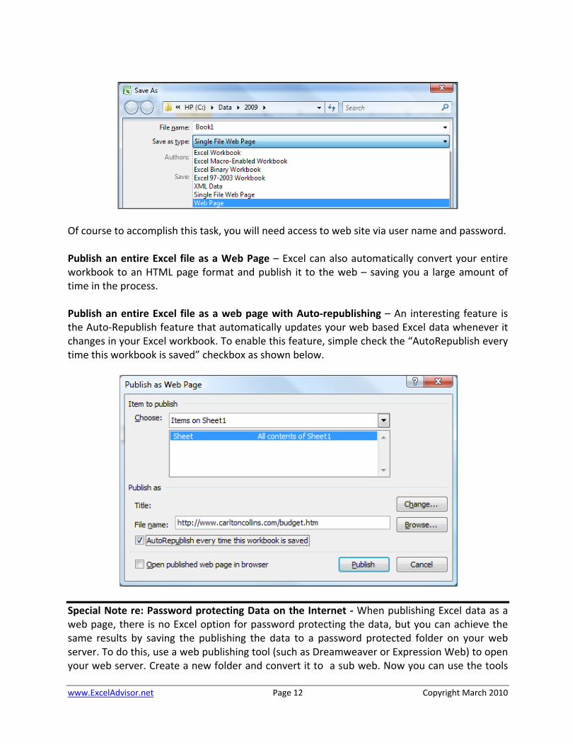
Publish Part of an Excel file as an Web Page – Excel enables you to publish a selection of cells as a web page in an HTML format. To do this, simply change the “Save As Type” to “Web Page” as shown in the screen below.
www.ExcelAdvisor.net Page 12 Copyright March 2010
Of course to accomplish this task, you will need access to web site via user name and password. Publish an entire Excel file as a Web Page – Excel can also automatically convert your entire workbook to an HTML page format and publish it to the web – saving you a large amount of time in the process. Publish an entire Excel file as a web page with Auto‐republishing – An interesting feature is the Auto‐Republish feature that automatically updates your web based Excel data whenever it changes in your Excel workbook. To enable this feature, simple check the “AutoRepublish every time this workbook is saved” checkbox as shown below.
Special Note re: Password protecting Data on the Internet ‐ When publishing Excel data as a web page, there is no Excel option for password protecting the data, but you can achieve the same results by saving the publishing the data to a password protected folder on your web server. To do this, use a web publishing tool (such as Dreamweaver or Expression Web) to open your web server. Create a new folder and convert it to a sub web. Now you can use the tools

www.ExcelAdvisor.net Page 13 Copyright March 2010
options to apply permissions to that folder. (Caveat – only UNIX based web servers allow you to apply these type of permissions, Windows based web servers do not). Web Queries ‐ Excel includes pre‐designed “queries” that can import commonly used data in 10 seconds. For example, you could use a web query to create a stock portfolio. All you need is a connection to the Internet and of course, some stock ticker symbols. In Excel 2003 select “Data, Import External Data, Import Data” and walk through the web query wizard for importing stock quotes. In Excel 2007 and later use the Data Ribbon, Existing Connections, Stock Quotes option. In seconds, Excel will retrieve 20 minute delayed stock prices from the web (during the hours when the stock market is open) and display a grid of complete up‐to‐date stick price information that is synchronized to the stock market’s changing stock prices. With each click of the “Refresh” button, the stock price information in Excel is updated ‐ this sure beats picking numbers out of the newspaper.
Completing the Stock Portfolio – Next link the grid data to another worksheet, and insert new columns containing the number of shares owned, as wells as an additional column to computer the total value based on shares owned, as shown below.
www.ExcelAdvisor.net Page 14 Copyright March 2010
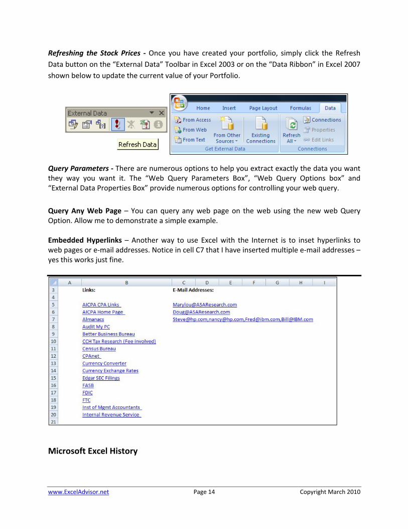
Refreshing the Stock Prices ‐ Once you have created your portfolio, simply click the Refresh Data button on the “External Data” Toolbar in Excel 2003 or on the “Data Ribbon” in Excel 2007 shown below to update the current value of your Portfolio.
Query Parameters ‐ There are numerous options to help you extract exactly the data you want they way you want it. The “Web Query Parameters Box”, “Web Query Options box” and “External Data Properties Box” provide numerous options for controlling your web query.
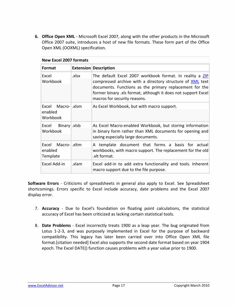
Query Any Web Page – You can query any web page on the web using the new web Query Option. Allow me to demonstrate a simple example. Embedded Hyperlinks – Another way to use Excel with the Internet is to inset hyperlinks to web pages or e‐mail addresses. Notice in cell C7 that I have inserted multiple e‐mail addresses – yes this works just fine.
Microsoft Excel History

www.ExcelAdvisor.net Page 15 Copyright March 2010
Microsoft began selling a spreadsheet application called Multiplan in 1982 for CP/M systems like the Osboune computer. However, on the MS‐DOS platform Lotus 1‐2‐3 was the market leader. Microsoft released Excel for the Mac in 1985, and Excel for Windows version in November, 1987. Lotus was slow to release a Windows version of 1‐2‐3 and by 1988 Excel was outselling 1‐2‐3. Later IBM purchased Lotus Development Corporation and is typical with software owned by IBM, the product’s presence diminished in the marketplace. Officially the current version for the Windows platform is Excel 12, also called Microsoft Office Excel 2007. The current version for the Mac OS X platform is Microsoft Excel 2008.
Microsoft Excel 2.1 included a runtime version of Windows 2.1 A Few Comments about Excel:
1. Trademark Dispute ‐ In 1993, another company that was already selling a software
package named "Excel" in the finance industry Excel became filed a trademark lawsuit. Eventually, this forced Microsoft to refer to the program as "Microsoft Excel". Later Microsoft purchased the trademark rights.
2. Formatting ‐ Excel was the first electronic spreadsheet that allowed the user to define the appearance of spreadsheets (fonts, character attributes and cell appearance).
3. Recomputation ‐ It also introduced intelligent cell recomputation, where only cells dependent on the cell being modified are updated (previous spreadsheet programs recomputed everything all the time or waited for a specific user command).

www.ExcelAdvisor.net Page 16 Copyright March 2010
4. VBA ‐ Since 1993, Excel has included Visual Basic for Applications (VBA), a programming language based on Visual Basic which adds the ability to automate tasks in Excel and to provide user defined functions (UDF) for use in worksheets. VBA allows the creation of forms and in‐worksheet controls to communicate with the user. The language supports use (but not creation) of ActiveX (COM) DLL's; later versions add support for class modules allowing the use of basic object‐oriented programming techniques.
File Formats ‐ Until 2007 Microsoft Excel used a proprietary binary file format called Binary Interchange File Format (BIFF) as its primary format. Excel 2007 uses Office Open XML as its primary file format, an XML‐based format that followed after a previous XML‐based format called "XML Spreadsheet" ("XMLSS"), first introduced in Excel 2002. The latter format is not able to encode VBA macros. Although supporting and encouraging the use of new XML‐based formats as replacements, Excel 2007 remained backwards‐compatible with the traditional, binary formats. In addition, most versions of Microsoft Excel can read CSV, DBF, SYLK, DIF, and other legacy formats. Support for some older file formats were removed in Excel 2007. The file formats were mainly from DOS based programs.
5. Binary ‐ Microsoft made the specification of the Excel binary format specification
available on request, but since February 2008 programmers can freely download the .XLS format specification and implement it under the Open Specification Promise patent licensing.[
Standard file‐extensions:
Format Extension Description
Spreadsheet .xls Main spreadsheet format which holds data in worksheets, charts, and macros
Add‐in (VBA)
.xla Adds custom functionality; written in VBA
Toolbar .xlb
Chart .xlc
Dialog .xld
Archive .xlk
Add‐in (DLL) .xll Adds custom functionality; written in C++/C, Visual Basic, Fortran, etc. and compiled in to a special dynamic‐link library
Macro .xlm
Template .xlt
Module .xlv
Workspace .xlw Arrangement of the windows of multiple Workbooks
www.ExcelAdvisor.net Page 17 Copyright March 2010
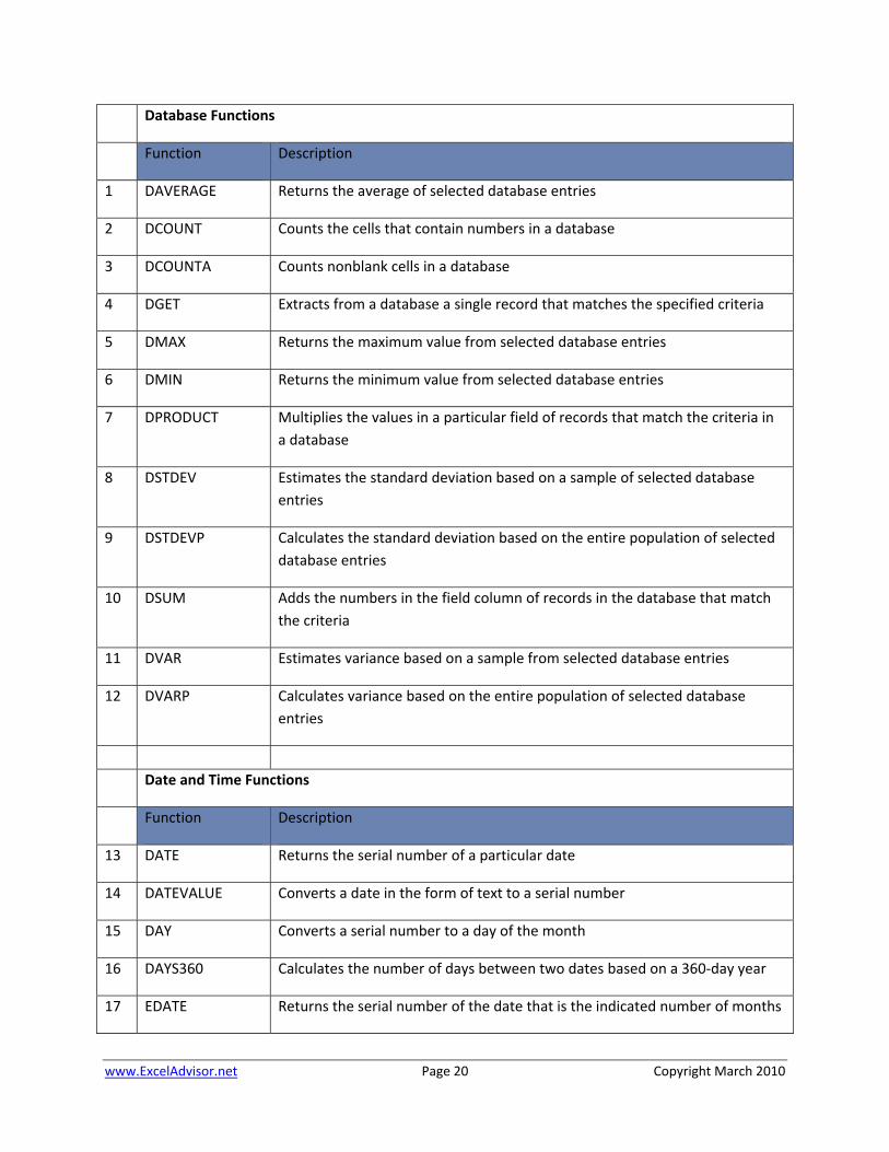
6. Office Open XML ‐ Microsoft Excel 2007, along with the other products in the Microsoft
Office 2007 suite, introduces a host of new file formats. These form part of the Office Open XML (OOXML) specification.
New Excel 2007 formats
Format Extension Description
Excel Workbook
.xlsx The default Excel 2007 workbook format. In reality a ZIPcompressed archive with a directory structure of XML text documents. Functions as the primary replacement for the former binary .xls format, although it does not support Excel macros for security reasons.
Excel Macro‐enabled Workbook
.xlsm As Excel Workbook, but with macro support.
Excel Binary Workbook
.xlsb As Excel Macro‐enabled Workbook, but storing information in binary form rather than XML documents for opening and saving especially large documents.
Excel Macro‐enabled Template
.xltm A template document that forms a basis for actual workbooks, with macro support. The replacement for the old .xlt format.
Excel Add‐in .xlam Excel add‐in to add extra functionality and tools. Inherent macro support due to the file purpose.
Software Errors ‐ Criticisms of spreadsheets in general also apply to Excel. See Spreadsheet shortcomings. Errors specific to Excel include accuracy, date problems and the Excel 2007 display error.
7. Accuracy ‐ Due to Excel's foundation on floating point calculations, the statistical accuracy of Excel has been criticized as lacking certain statistical tools.
8. Date Problems ‐ Excel incorrectly treats 1900 as a leap year. The bug originated from
Lotus 1‐2‐3, and was purposely implemented in Excel for the purpose of backward compatibility. This legacy has later been carried over into Office Open XML file format.[citation needed] Excel also supports the second date format based on year 1904 epoch. The Excel DATE() function causes problems with a year value prior to 1900.

www.ExcelAdvisor.net Page 18 Copyright March 2010
Chapter 3
Functions

www.ExcelAdvisor.net Page 19 Copyright March 2010
Introduction to Excel Functions
Excel Functions are preprogrammed commands that make the task of writing complex formulas easier. There are a total of 333 functions in Excel. These functions are separated into 11 categories as follows:
1. Database Functions (12) 2. Date and Time Functions (20) 3. Engineering Functions (39) 4. Financial Functions (53) 5. Information Functions (17) 6. Logical Functions (6) 7. Lookup and Reference Functions (18) 8. Math and Trigonometry Functions (59) 9. Statistical Functions (80) 10. Text Functions (27) 11. External Functions (2)
Some Excel functions are more powerful than others and some are more relevant to the CPA than others. For example, most CPAs will find the IF, SUM, COUNT, SUBTOTAL, TEXT, and VLOOKUP are very relevant to the CPA while other engineering and trigonometry functions such as LOG, PI, RADIENS, DELTA, TAN, COMPLEX, and HAX2DEC are typically less relevant to CPAs. It has been my experience that the following 67 functions are most relevant to the CPA; therefore CPAs wishing to increase their command of Excel functions should concentrate on these functions first.
Carlton’s List of The Top 67 Functions Most Relevant to CPAs Sorted By Carlton’s Opinion of the Most Useful
1. IF 2. SUM 3. SUMIF 4. COUNT 5. COUNTA
6. AVERAGE 7. COUNTBLANK 8. COUNTIF 9. VALUE 10. TEXT 11. VLOOKUP 12. HLOOKUP 13. LOOKUP 14. TRIM 15. PROPER16. LOWER 17. LEFT, LEFTB 18. MID, MIDB 19. RIGHT, 20. FIND, FINDB21. REPLACE 22. CONCATENATE 23. CLEAN 24. UPPER 25. LEN, LENB26. SUBSTITUTE 27. NOW 28. TODAY 29. MONTH 30. DATE31. DAY 32. YEAR 33. WEEKDAY 34. ROUND 35. ROUNDDOWN
36. ROUNDUP 37. MAX 38. MIN 39. MEDIAN 40. MODE
41. PERCENTILE 42. PERCENTRANK 43. PMT 44. NPV 45. DSUM46. DCOUNT 47. DCOUNTA 48. AND 49. OR 50. CHOOSE51. TIME 52. FV 53. IRR 54. YIELD 55. CELL 56. ERROR.TYPE 57. INFO 58. ISBLANK 59. ISNA 60. GETPIVOTDATA61. HYPERLINK 62. TRANSPOSE 63. ABS 64. RAND 65. RANDBETWEEN
66. CONFIDENCE 67. REPT
Following is a list of all Excel functions, organized by category, including a description of each function.
www.ExcelAdvisor.net Page 20 Copyright March 2010
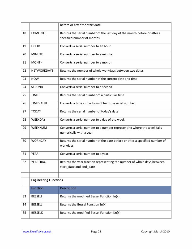
Database Functions
Function Description
1 DAVERAGE Returns the average of selected database entries
2 DCOUNT Counts the cells that contain numbers in a database
3 DCOUNTA Counts nonblank cells in a database
4 DGET Extracts from a database a single record that matches the specified criteria
5 DMAX Returns the maximum value from selected database entries
6 DMIN Returns the minimum value from selected database entries
7 DPRODUCT Multiplies the values in a particular field of records that match the criteria in a database
8 DSTDEV Estimates the standard deviation based on a sample of selected database entries
9 DSTDEVP Calculates the standard deviation based on the entire population of selected database entries
10 DSUM Adds the numbers in the field column of records in the database that match the criteria
11 DVAR Estimates variance based on a sample from selected database entries
12 DVARP Calculates variance based on the entire population of selected database entries
Date and Time Functions
Function Description
13 DATE Returns the serial number of a particular date
14 DATEVALUE Converts a date in the form of text to a serial number
15 DAY Converts a serial number to a day of the month
16 DAYS360 Calculates the number of days between two dates based on a 360‐day year
17 EDATE Returns the serial number of the date that is the indicated number of months
www.ExcelAdvisor.net Page 21 Copyright March 2010
before or after the start date
18 EOMONTH Returns the serial number of the last day of the month before or after a specified number of months
19 HOUR Converts a serial number to an hour
20 MINUTE Converts a serial number to a minute
21 MONTH Converts a serial number to a month
22 NETWORKDAYS Returns the number of whole workdays between two dates
23 NOW Returns the serial number of the current date and time
24 SECOND Converts a serial number to a second
25 TIME Returns the serial number of a particular time
26 TIMEVALUE Converts a time in the form of text to a serial number
27 TODAY Returns the serial number of today's date
28 WEEKDAY Converts a serial number to a day of the week
29 WEEKNUM Converts a serial number to a number representing where the week falls numerically with a year
30 WORKDAY Returns the serial number of the date before or after a specified number of workdays
31 YEAR Converts a serial number to a year
32 YEARFRAC Returns the year fraction representing the number of whole days between start_date and end_date
Engineering Functions
Function Description
33 BESSELI Returns the modified Bessel Function In(x)
34 BESSELJ Returns the Bessel Function Jn(x)
35 BESSELK Returns the modified Bessel Function Kn(x)

www.ExcelAdvisor.net Page 22 Copyright March 2010
36 BESSELY Returns the Bessel Function Yn(x)
37 BIN2DEC Converts a binary number to decimal
38 BIN2HEX Converts a binary number to hexadecimal
39 BIN2OCT Converts a binary number to octal
40 COMPLEX Converts real and imaginary coefficients into a complex number
41 CONVERT Converts a number from one measurement system to another
42 DEC2BIN Converts a decimal number to binary
43 DEC2HEX Converts a decimal number to hexadecimal
44 DEC2OCT Converts a decimal number to octal
45 DELTA Tests whether two values are equal
46 ERF Returns the error Function
47 ERFC Returns the complementary error Function
48 GESTEP Tests whether a number is greater than a threshold value
49 HEX2BIN Converts a hexadecimal number to binary
50 HEX2DEC Converts a hexadecimal number to decimal
51 HEX2OCT Converts a hexadecimal number to octal
52 IMABS Returns the absolute value (modulus) of a complex number
53 IMAGINARY Returns the imaginary coefficient of a complex number
54 IMARGUMENT Returns the argument theta, an angle expressed in radians
55 IMCONJUGATE Returns the complex conjugate of a complex number
56 IMCOS Returns the cosine of a complex number
57 IMDIV Returns the quotient of two complex numbers
58 IMEXP Returns the exponential of a complex number
59 IMLN Returns the natural logarithm of a complex number
www.ExcelAdvisor.net Page 23 Copyright March 2010
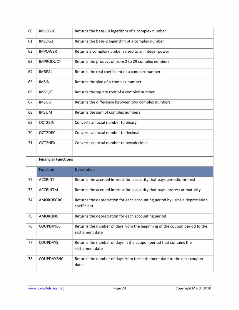
60 IMLOG10 Returns the base‐10 logarithm of a complex number
61 IMLOG2 Returns the base‐2 logarithm of a complex number
62 IMPOWER Returns a complex number raised to an integer power
63 IMPRODUCT Returns the product of from 2 to 29 complex numbers
64 IMREAL Returns the real coefficient of a complex number
65 IMSIN Returns the sine of a complex number
66 IMSQRT Returns the square root of a complex number
67 IMSUB Returns the difference between two complex numbers
68 IMSUM Returns the sum of complex numbers
69 OCT2BIN Converts an octal number to binary
70 OCT2DEC Converts an octal number to decimal
71 OCT2HEX Converts an octal number to hexadecimal
Financial Functions
Function Description
72 ACCRINT Returns the accrued interest for a security that pays periodic interest
73 ACCRINTM Returns the accrued interest for a security that pays interest at maturity
74 AMORDEGRC Returns the depreciation for each accounting period by using a depreciation coefficient
75 AMORLINC Returns the depreciation for each accounting period
76 COUPDAYBS Returns the number of days from the beginning of the coupon period to the settlement date
77 COUPDAYS Returns the number of days in the coupon period that contains the settlement date
78 COUPDAYSNC Returns the number of days from the settlement date to the next coupon date
www.ExcelAdvisor.net Page 24 Copyright March 2010
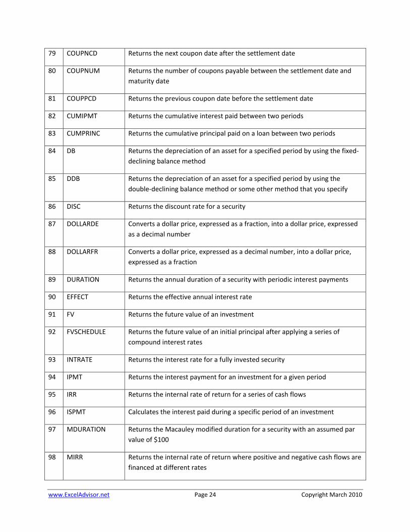
79 COUPNCD Returns the next coupon date after the settlement date
80 COUPNUM Returns the number of coupons payable between the settlement date and maturity date
81 COUPPCD Returns the previous coupon date before the settlement date
82 CUMIPMT Returns the cumulative interest paid between two periods
83 CUMPRINC Returns the cumulative principal paid on a loan between two periods
84 DB Returns the depreciation of an asset for a specified period by using the fixed‐declining balance method
85 DDB Returns the depreciation of an asset for a specified period by using the double‐declining balance method or some other method that you specify
86 DISC Returns the discount rate for a security
87 DOLLARDE Converts a dollar price, expressed as a fraction, into a dollar price, expressed as a decimal number
88 DOLLARFR Converts a dollar price, expressed as a decimal number, into a dollar price, expressed as a fraction
89 DURATION Returns the annual duration of a security with periodic interest payments
90 EFFECT Returns the effective annual interest rate
91 FV Returns the future value of an investment
92 FVSCHEDULE Returns the future value of an initial principal after applying a series of compound interest rates
93 INTRATE Returns the interest rate for a fully invested security
94 IPMT Returns the interest payment for an investment for a given period
95 IRR Returns the internal rate of return for a series of cash flows
96 ISPMT Calculates the interest paid during a specific period of an investment
97 MDURATION Returns the Macauley modified duration for a security with an assumed par value of $100
98 MIRR Returns the internal rate of return where positive and negative cash flows are financed at different rates
www.ExcelAdvisor.net Page 25 Copyright March 2010
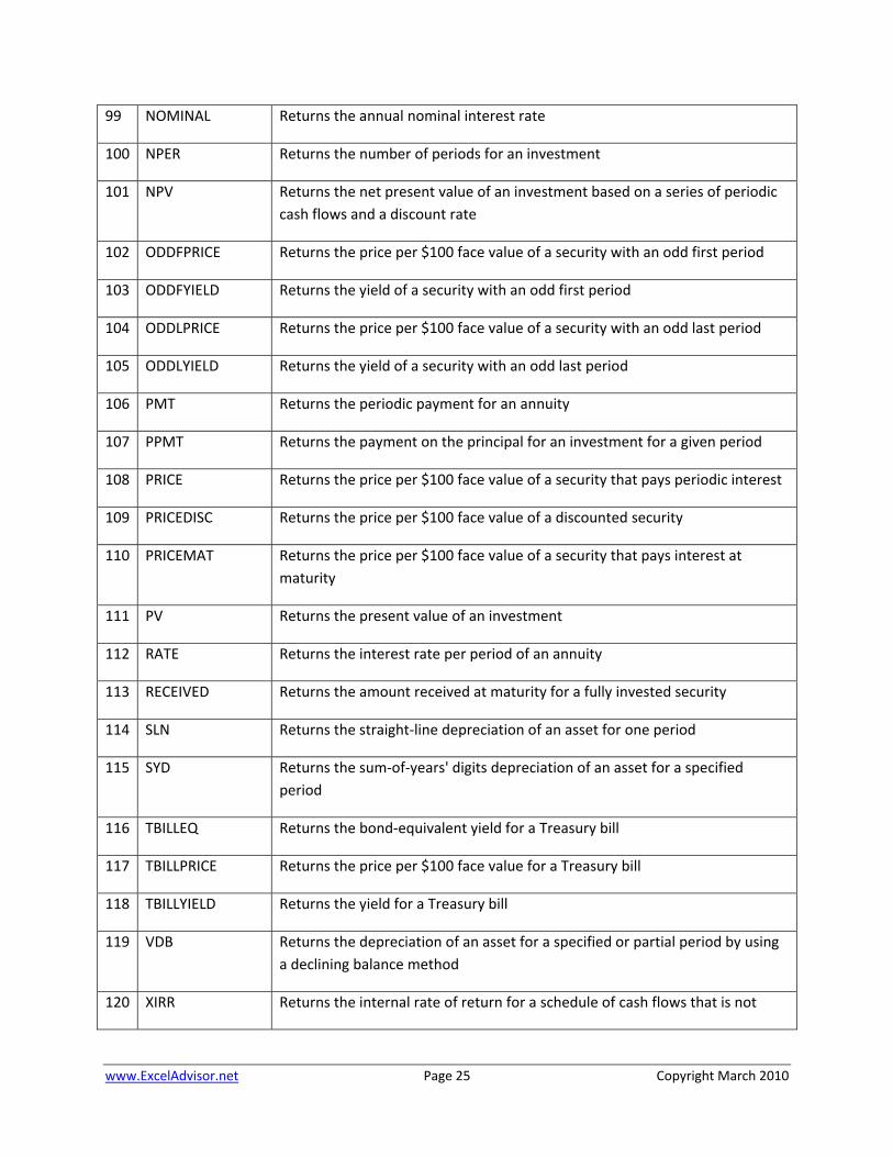
99 NOMINAL Returns the annual nominal interest rate
100 NPER Returns the number of periods for an investment
101 NPV Returns the net present value of an investment based on a series of periodic cash flows and a discount rate
102 ODDFPRICE Returns the price per $100 face value of a security with an odd first period
103 ODDFYIELD Returns the yield of a security with an odd first period
104 ODDLPRICE Returns the price per $100 face value of a security with an odd last period
105 ODDLYIELD Returns the yield of a security with an odd last period
106 PMT Returns the periodic payment for an annuity
107 PPMT Returns the payment on the principal for an investment for a given period
108 PRICE Returns the price per $100 face value of a security that pays periodic interest
109 PRICEDISC Returns the price per $100 face value of a discounted security
110 PRICEMAT Returns the price per $100 face value of a security that pays interest at maturity
111 PV Returns the present value of an investment
112 RATE Returns the interest rate per period of an annuity
113 RECEIVED Returns the amount received at maturity for a fully invested security
114 SLN Returns the straight‐line depreciation of an asset for one period
115 SYD Returns the sum‐of‐years' digits depreciation of an asset for a specified period
116 TBILLEQ Returns the bond‐equivalent yield for a Treasury bill
117 TBILLPRICE Returns the price per $100 face value for a Treasury bill
118 TBILLYIELD Returns the yield for a Treasury bill
119 VDB Returns the depreciation of an asset for a specified or partial period by using a declining balance method
120 XIRR Returns the internal rate of return for a schedule of cash flows that is not

www.ExcelAdvisor.net Page 26 Copyright March 2010
necessarily periodic
121 XNPV Returns the net present value for a schedule of cash flows that is not necessarily periodic
122 YIELD Returns the yield on a security that pays periodic interest
123 YIELDDISC Returns the annual yield for a discounted security; for example, a Treasury bill
124 YIELDMAT Returns the annual yield of a security that pays interest at maturity
Information Functions
Function Description
125 CELL Returns information about the formatting, location, or contents of a cell
126 ERROR.TYPE Returns a number corresponding to an error type
127 INFO Returns information about the current operating environment
128 ISBLANK Returns TRUE if the value is blank
129 ISERR Returns TRUE if the value is any error value except #N/A
130 ISERROR Returns TRUE if the value is any error value
131 ISEVEN Returns TRUE if the number is even
132 ISLOGICAL Returns TRUE if the value is a logical value
133 ISNA Returns TRUE if the value is the #N/A error value
134 ISNONTEXT Returns TRUE if the value is not text
135 ISNUMBER Returns TRUE if the value is a number
136 ISODD Returns TRUE if the number is odd
137 ISREF Returns TRUE if the value is a reference
138 ISTEXT Returns TRUE if the value is text
139 N Returns a value converted to a number
140 NA Returns the error value #N/A
www.ExcelAdvisor.net Page 27 Copyright March 2010
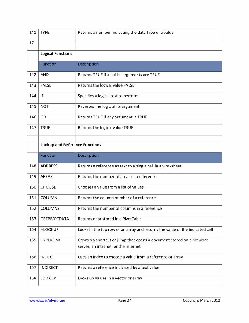
141 TYPE Returns a number indicating the data type of a value
17
Logical Functions
Function Description
142 AND Returns TRUE if all of its arguments are TRUE
143 FALSE Returns the logical value FALSE
144 IF Specifies a logical test to perform
145 NOT Reverses the logic of its argument
146 OR Returns TRUE if any argument is TRUE
147 TRUE Returns the logical value TRUE
Lookup and Reference Functions
Function Description
148 ADDRESS Returns a reference as text to a single cell in a worksheet
149 AREAS Returns the number of areas in a reference
150 CHOOSE Chooses a value from a list of values
151 COLUMN Returns the column number of a reference
152 COLUMNS Returns the number of columns in a reference
153 GETPIVOTDATA Returns data stored in a PivotTable
154 HLOOKUP Looks in the top row of an array and returns the value of the indicated cell
155 HYPERLINK Creates a shortcut or jump that opens a document stored on a network server, an intranet, or the Internet
156 INDEX Uses an index to choose a value from a reference or array
157 INDIRECT Returns a reference indicated by a text value
158 LOOKUP Looks up values in a vector or array

www.ExcelAdvisor.net Page 28 Copyright March 2010
159 MATCH Looks up values in a reference or array
160 OFFSET Returns a reference offset from a given reference
161 ROW Returns the row number of a reference
162 ROWS Returns the number of rows in a reference
163 RTD Retrieves real‐time data from a program that supports COM automation (Automation: A way to work with an application's objects from another application or development tool. Formerly called OLE Automation, Automation is an industry standard and a feature of the Component Object Model (COM).)
164 TRANSPOSE Returns the transpose of an array
165 VLOOKUP Looks in the first column of an array and moves across the row to return the value of a cell
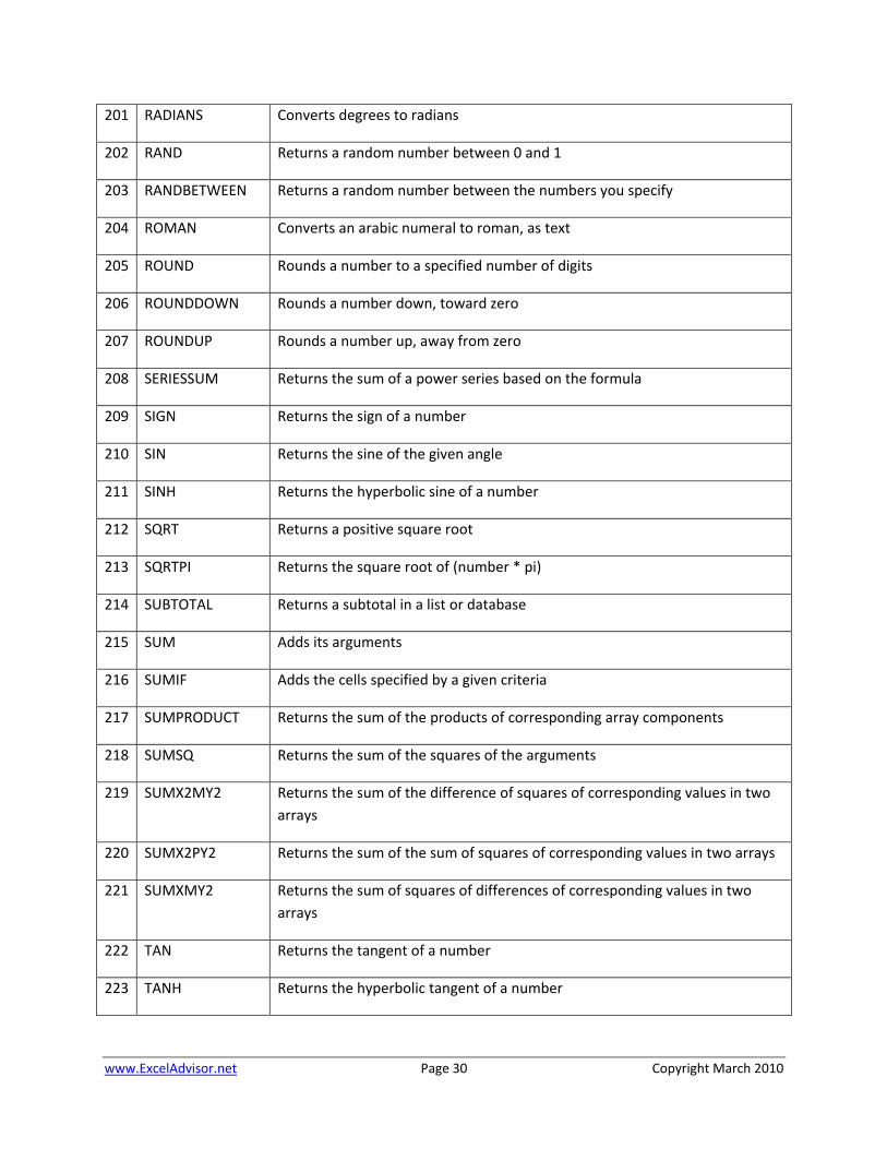
Math and Trigonometry Functions
Function Description
166 ABS Returns the absolute value of a number
167 ACOS Returns the arccosine of a number
168 ACOSH Returns the inverse hyperbolic cosine of a number
169 ASIN Returns the arcsine of a number
170 ASINH Returns the inverse hyperbolic sine of a number
171 ATAN Returns the arctangent of a number
172 ATAN2 Returns the arctangent from x‐ and y‐coordinates
173 ATANH Returns the inverse hyperbolic tangent of a number
174 CEILING Rounds a number to the nearest integer or to the nearest multiple of significance
175 COMBIN Returns the number of combinations for a given number of objects
176 COS Returns the cosine of a number

www.ExcelAdvisor.net Page 29 Copyright March 2010
177 COSH Returns the hyperbolic cosine of a number
178 DEGREES Converts radians to degrees
179 EVEN Rounds a number up to the nearest even integer
180 EXP Returns e raised to the power of a given number
181 FACT Returns the factorial of a number
182 FACTDOUBLE Returns the double factorial of a number
183 FLOOR Rounds a number down, toward zero
184 GCD Returns the greatest common divisor
185 INT Rounds a number down to the nearest integer
186 LCM Returns the least common multiple
187 LN Returns the natural logarithm of a number
188 LOG Returns the logarithm of a number to a specified base
189 LOG10 Returns the base‐10 logarithm of a number
190 MDETERM Returns the matrix determinant of an array
191 MINVERSE Returns the matrix inverse of an array
192 MMULT Returns the matrix product of two arrays
193 MOD Returns the remainder from division
194 MROUND Returns a number rounded to the desired multiple
195 MULTINOMIAL Returns the multinomial of a set of numbers
196 ODD Rounds a number up to the nearest odd integer
197 PI Returns the value of pi
198 POWER Returns the result of a number raised to a power
199 PRODUCT Multiplies its arguments
200 QUOTIENT Returns the integer portion of a division
www.ExcelAdvisor.net Page 30 Copyright March 2010
201 RADIANS Converts degrees to radians
202 RAND Returns a random number between 0 and 1
203 RANDBETWEEN Returns a random number between the numbers you specify
204 ROMAN Converts an arabic numeral to roman, as text
205 ROUND Rounds a number to a specified number of digits
206 ROUNDDOWN Rounds a number down, toward zero
207 ROUNDUP Rounds a number up, away from zero
208 SERIESSUM Returns the sum of a power series based on the formula
209 SIGN Returns the sign of a number
210 SIN Returns the sine of the given angle
211 SINH Returns the hyperbolic sine of a number
212 SQRT Returns a positive square root
213 SQRTPI Returns the square root of (number * pi)
214 SUBTOTAL Returns a subtotal in a list or database
215 SUM Adds its arguments
216 SUMIF Adds the cells specified by a given criteria
217 SUMPRODUCT Returns the sum of the products of corresponding array components
218 SUMSQ Returns the sum of the squares of the arguments
219 SUMX2MY2 Returns the sum of the difference of squares of corresponding values in two arrays
220 SUMX2PY2 Returns the sum of the sum of squares of corresponding values in two arrays
221 SUMXMY2 Returns the sum of squares of differences of corresponding values in two arrays
222 TAN Returns the tangent of a number
223 TANH Returns the hyperbolic tangent of a number
www.ExcelAdvisor.net Page 31 Copyright March 2010
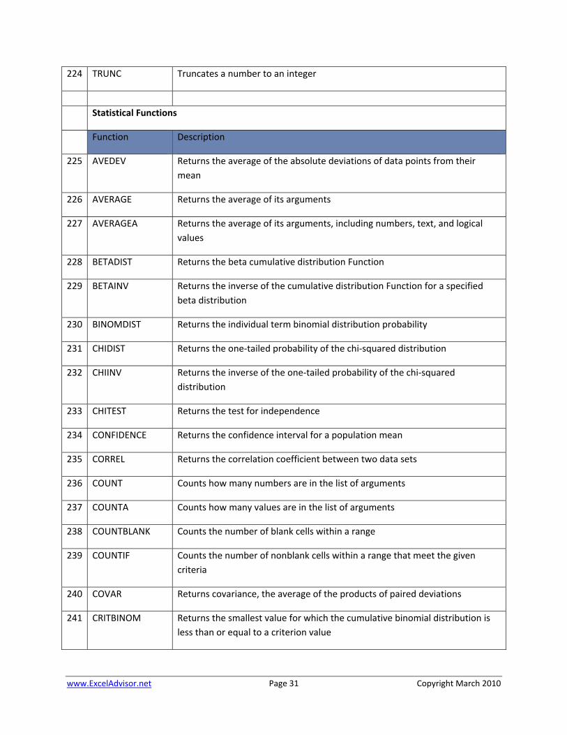
224 TRUNC Truncates a number to an integer
Statistical Functions
Function Description
225 AVEDEV Returns the average of the absolute deviations of data points from their mean
226 AVERAGE Returns the average of its arguments
227 AVERAGEA Returns the average of its arguments, including numbers, text, and logical values
228 BETADIST Returns the beta cumulative distribution Function
229 BETAINV Returns the inverse of the cumulative distribution Function for a specified beta distribution
230 BINOMDIST Returns the individual term binomial distribution probability
231 CHIDIST Returns the one‐tailed probability of the chi‐squared distribution
232 CHIINV Returns the inverse of the one‐tailed probability of the chi‐squared distribution
233 CHITEST Returns the test for independence
234 CONFIDENCE Returns the confidence interval for a population mean
235 CORREL Returns the correlation coefficient between two data sets
236 COUNT Counts how many numbers are in the list of arguments
237 COUNTA Counts how many values are in the list of arguments
238 COUNTBLANK Counts the number of blank cells within a range
239 COUNTIF Counts the number of nonblank cells within a range that meet the given criteria
240 COVAR Returns covariance, the average of the products of paired deviations
241 CRITBINOM Returns the smallest value for which the cumulative binomial distribution is less than or equal to a criterion value
www.ExcelAdvisor.net Page 32 Copyright March 2010
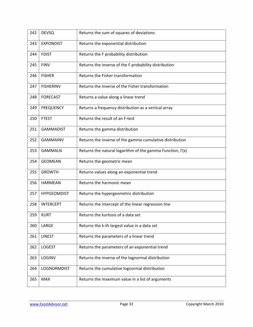
242 DEVSQ Returns the sum of squares of deviations
243 EXPONDIST Returns the exponential distribution
244 FDIST Returns the F probability distribution
245 FINV Returns the inverse of the F probability distribution
246 FISHER Returns the Fisher transformation
247 FISHERINV Returns the inverse of the Fisher transformation
248 FORECAST Returns a value along a linear trend
249 FREQUENCY Returns a frequency distribution as a vertical array
250 FTEST Returns the result of an F‐test
251 GAMMADIST Returns the gamma distribution
252 GAMMAINV Returns the inverse of the gamma cumulative distribution
253 GAMMALN Returns the natural logarithm of the gamma Function, Γ(x)
254 GEOMEAN Returns the geometric mean
255 GROWTH Returns values along an exponential trend
256 HARMEAN Returns the harmonic mean
257 HYPGEOMDIST Returns the hypergeometric distribution
258 INTERCEPT Returns the intercept of the linear regression line
259 KURT Returns the kurtosis of a data set
260 LARGE Returns the k‐th largest value in a data set
261 LINEST Returns the parameters of a linear trend
262 LOGEST Returns the parameters of an exponential trend
263 LOGINV Returns the inverse of the lognormal distribution
264 LOGNORMDIST Returns the cumulative lognormal distribution
265 MAX Returns the maximum value in a list of arguments
www.ExcelAdvisor.net Page 33 Copyright March 2010
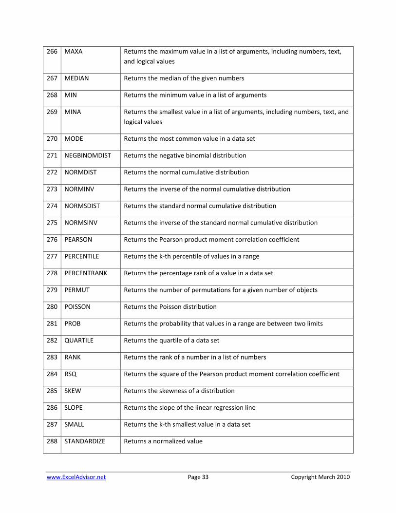
266 MAXA Returns the maximum value in a list of arguments, including numbers, text, and logical values
267 MEDIAN Returns the median of the given numbers
268 MIN Returns the minimum value in a list of arguments
269 MINA Returns the smallest value in a list of arguments, including numbers, text, and logical values
270 MODE Returns the most common value in a data set
271 NEGBINOMDIST Returns the negative binomial distribution
272 NORMDIST Returns the normal cumulative distribution
273 NORMINV Returns the inverse of the normal cumulative distribution
274 NORMSDIST Returns the standard normal cumulative distribution
275 NORMSINV Returns the inverse of the standard normal cumulative distribution
276 PEARSON Returns the Pearson product moment correlation coefficient
277 PERCENTILE Returns the k‐th percentile of values in a range
278 PERCENTRANK Returns the percentage rank of a value in a data set
279 PERMUT Returns the number of permutations for a given number of objects
280 POISSON Returns the Poisson distribution
281 PROB Returns the probability that values in a range are between two limits
282 QUARTILE Returns the quartile of a data set
283 RANK Returns the rank of a number in a list of numbers
284 RSQ Returns the square of the Pearson product moment correlation coefficient
285 SKEW Returns the skewness of a distribution
286 SLOPE Returns the slope of the linear regression line
287 SMALL Returns the k‐th smallest value in a data set
288 STANDARDIZE Returns a normalized value
www.ExcelAdvisor.net Page 34 Copyright March 2010
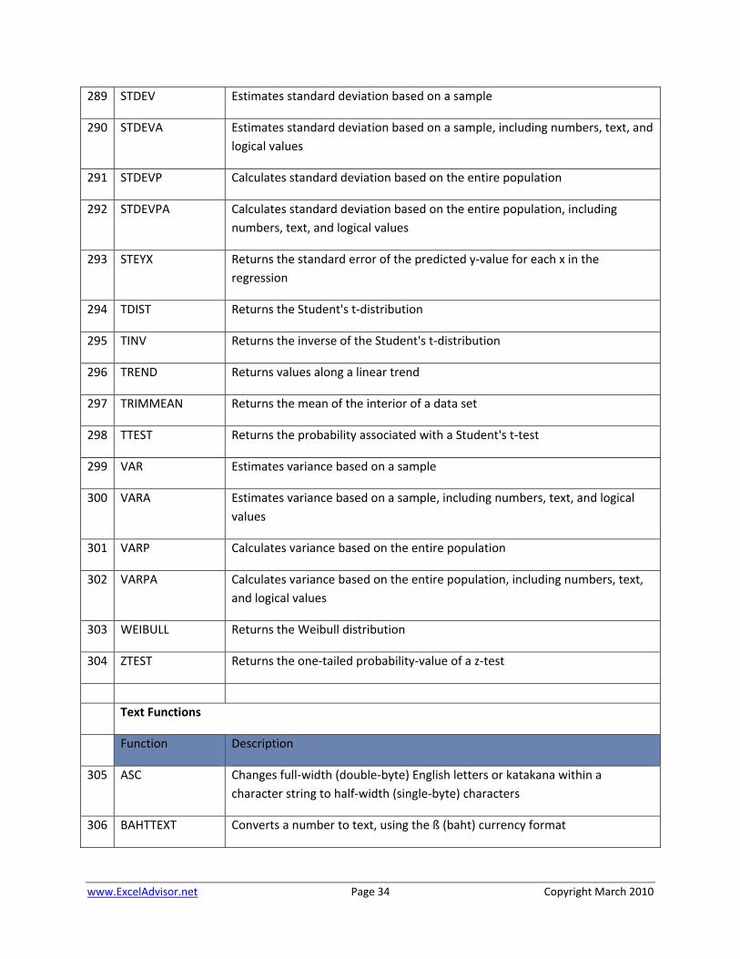
289 STDEV Estimates standard deviation based on a sample
290 STDEVA Estimates standard deviation based on a sample, including numbers, text, and logical values
291 STDEVP Calculates standard deviation based on the entire population
292 STDEVPA Calculates standard deviation based on the entire population, including numbers, text, and logical values
293 STEYX Returns the standard error of the predicted y‐value for each x in the regression
294 TDIST Returns the Student's t‐distribution
295 TINV Returns the inverse of the Student's t‐distribution
296 TREND Returns values along a linear trend
297 TRIMMEAN Returns the mean of the interior of a data set
298 TTEST Returns the probability associated with a Student's t‐test
299 VAR Estimates variance based on a sample
300 VARA Estimates variance based on a sample, including numbers, text, and logical values
301 VARP Calculates variance based on the entire population
302 VARPA Calculates variance based on the entire population, including numbers, text, and logical values
303 WEIBULL Returns the Weibull distribution
304 ZTEST Returns the one‐tailed probability‐value of a z‐test
Text Functions
Function Description
305 ASC Changes full‐width (double‐byte) English letters or katakana within a character string to half‐width (single‐byte) characters
306 BAHTTEXT Converts a number to text, using the ß (baht) currency format

www.ExcelAdvisor.net Page 35 Copyright March 2010
307 CHAR Returns the character specified by the code number
308 CLEAN Removes all nonprintable characters from text
309 CODE Returns a numeric code for the first character in a text string
310 CONCATENATE Joins several text items into one text item
311 DOLLAR Converts a number to text, using the $ (dollar) currency format
312 EXACT Checks to see if two text values are identical
313 FIND, FINDB Finds one text value within another (case‐sensitive)
314 FIXED Formats a number as text with a fixed number of decimals
315 JIS Changes half‐width (single‐byte) English letters or katakana within a character string to full‐width (double‐byte) characters
316 LEFT, LEFTB Returns the leftmost characters from a text value
317 LEN, LENB Returns the number of characters in a text string
318 LOWER Converts text to lowercase
319 MID, MIDB Returns a specific number of characters from a text string starting at the position you specify
320 PHONETIC Extracts the phonetic (furigana) characters from a text string
321 PROPER Capitalizes the first letter in each word of a text value
322 REPLACE, REPLACEB
Replaces characters within text
323 REPT Repeats text a given number of times
324 RIGHT, RIGHTB Returns the rightmost characters from a text value
325 SEARCH, SEARCHB
Finds one text value within another (not case‐sensitive)
326 SUBSTITUTE Substitutes new text for old text in a text string
327 T Converts its arguments to text
328 TEXT Formats a number and converts it to text

www.ExcelAdvisor.net Page 36 Copyright March 2010
329 TRIM Removes spaces from text
330 UPPER Converts text to uppercase
331 VALUE Converts a text argument to a number
External Functions
Function Description
332 EUROCONVERT Converts a number to euros, converts a number from euros to a euro member currency, or converts a number from one euro member currency to another by using the euro as an intermediary (triangulation)
333 SQL.REQUEST Connects with an external data source and runs a query from a worksheet, then returns the result as an array without the need for macro programming

www.ExcelAdvisor.net Page 37 Copyright March 2010
Chapter 4
The =IF Function
www.ExcelAdvisor.net Page 38 Copyright March 2010
=IF The “IF” function is the most powerful of all functions – not just in Excel, but in any programming language. Commonly referred to as “Conditional Programming”, it is the IF function that enables us to introduce logical thinking into any program. This function is also referred to as the “If‐Then‐Else” command, “conditional expressions”, or “Propositional Logic”. The following Wikis explains this concept in more detail:
http://en.wikipedia.org/wiki/Conditional_(programming). http://en.wikipedia.org/wiki/Logical_conditional#Conditional_statements
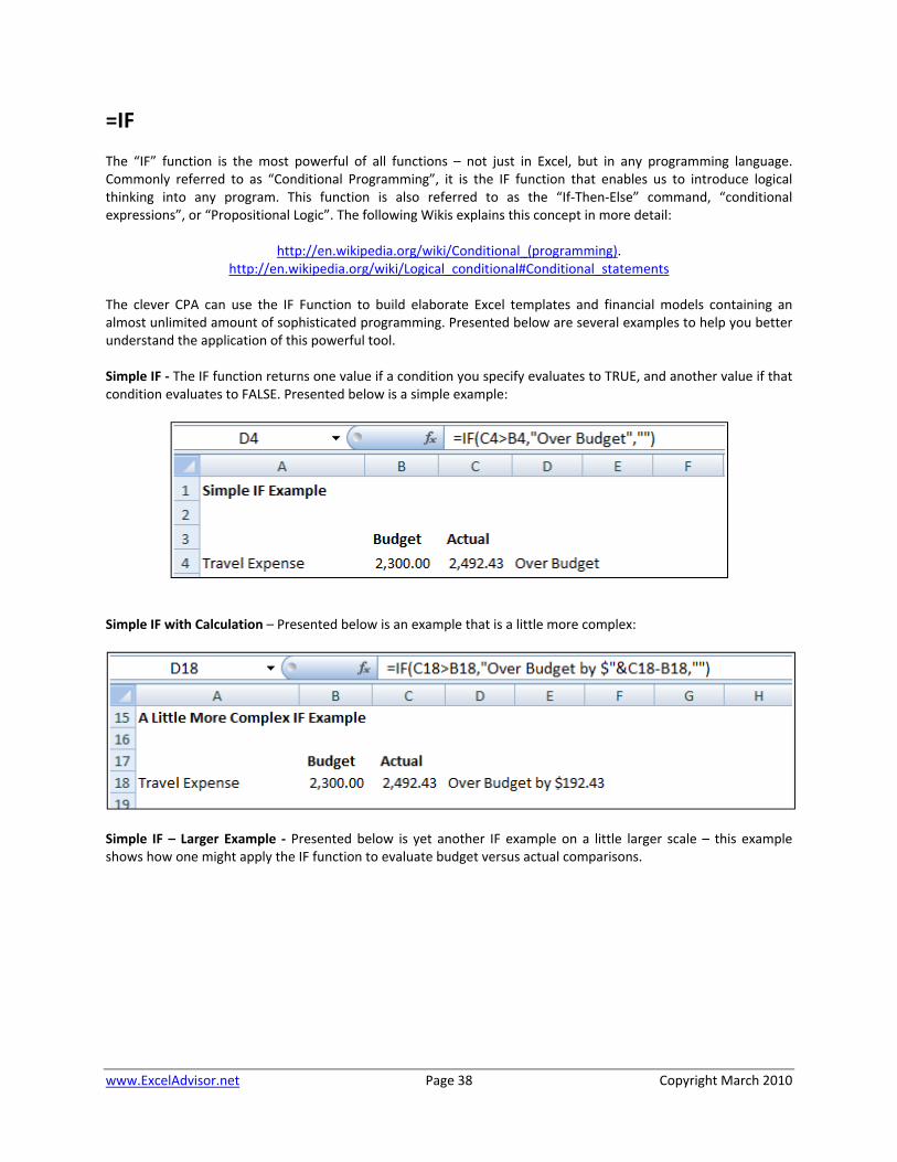
The clever CPA can use the IF Function to build elaborate Excel templates and financial models containing an almost unlimited amount of sophisticated programming. Presented below are several examples to help you better understand the application of this powerful tool. Simple IF ‐ The IF function returns one value if a condition you specify evaluates to TRUE, and another value if that condition evaluates to FALSE. Presented below is a simple example:
Simple IF with Calculation – Presented below is an example that is a little more complex:
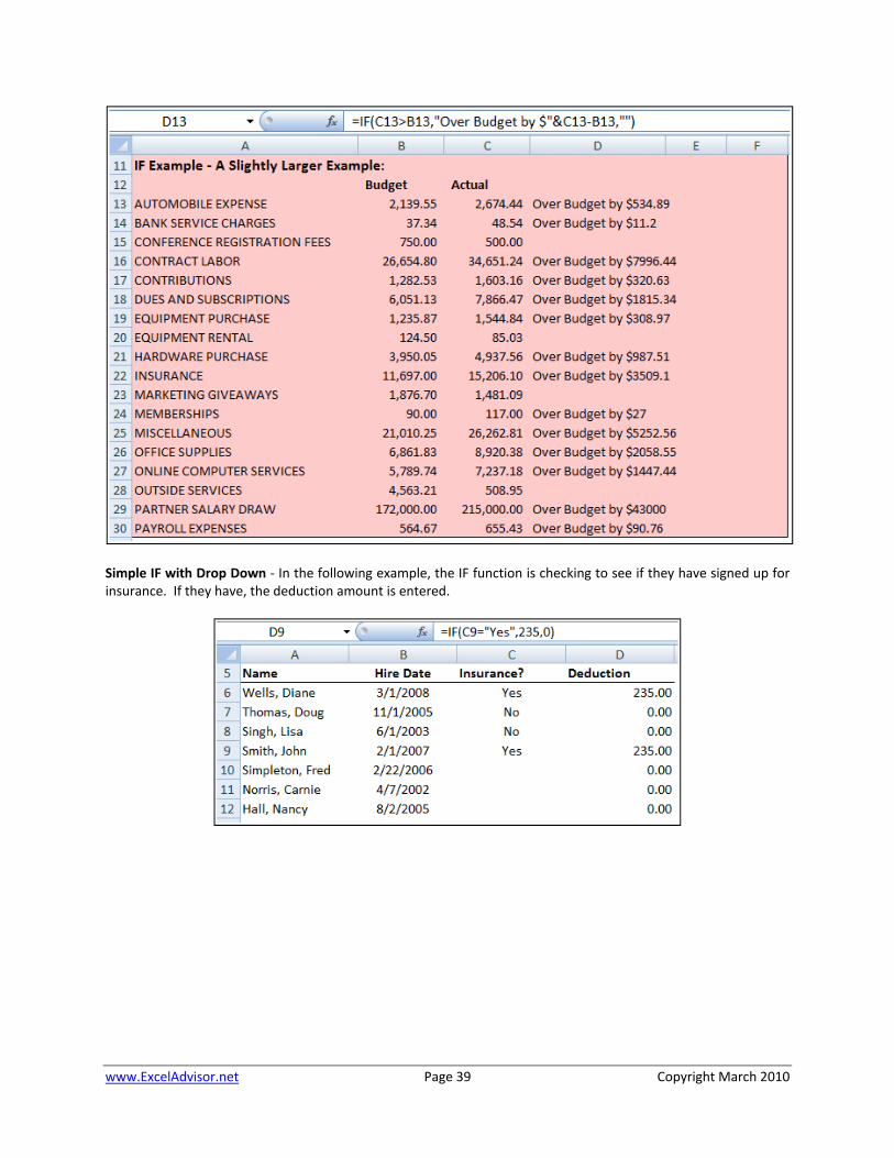
Simple IF – Larger Example ‐ Presented below is yet another IF example on a little larger scale – this example shows how one might apply the IF function to evaluate budget versus actual comparisons.
www.ExcelAdvisor.net Page 39 Copyright March 2010
Simple IF with Drop Down ‐ In the following example, the IF function is checking to see if they have signed up for insurance. If they have, the deduction amount is entered.
www.ExcelAdvisor.net Page 40 Copyright March 2010
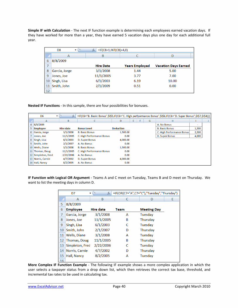
Simple IF with Calculation ‐ The next IF function example is determining each employees earned vacation days. If they have worked for more than a year, they have earned 5 vacation days plus one day for each additional full year.
Nested IF Functions ‐ In this sample, there are four possibilities for bonuses.
IF Function with Logical OR Argument ‐ Teams A and C meet on Tuesday, Teams B and D meet on Thursday. We want to list the meeting days in column D.
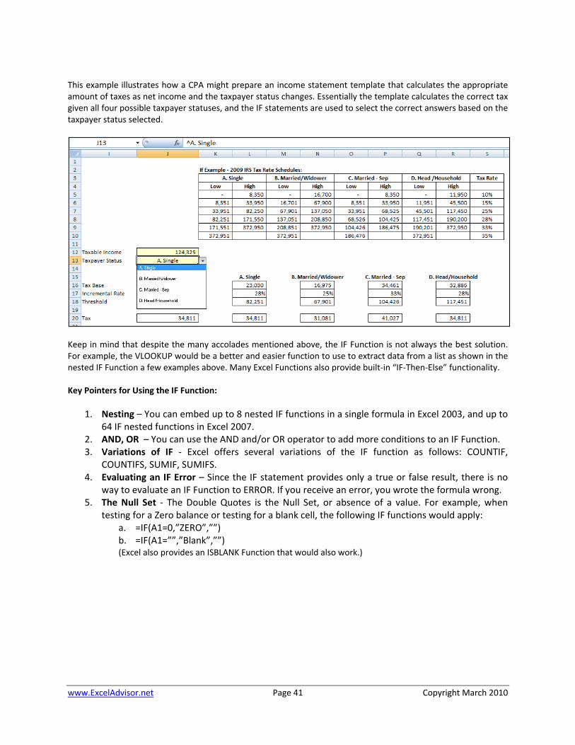
More Complex IF Function Example ‐ The following IF example shows a more complex application in which the user selects a taxpayer status from a drop down list, which then retrieves the correct tax base, threshold, and incremental tax rates to be used in calculating tax.
www.ExcelAdvisor.net Page 41 Copyright March 2010
This example illustrates how a CPA might prepare an income statement template that calculates the appropriate amount of taxes as net income and the taxpayer status changes. Essentially the template calculates the correct tax given all four possible taxpayer statuses, and the IF statements are used to select the correct answers based on the taxpayer status selected.
Keep in mind that despite the many accolades mentioned above, the IF Function is not always the best solution. For example, the VLOOKUP would be a better and easier function to use to extract data from a list as shown in the nested IF Function a few examples above. Many Excel Functions also provide built‐in “IF‐Then‐Else” functionality. Key Pointers for Using the IF Function:
1. Nesting – You can embed up to 8 nested IF functions in a single formula in Excel 2003, and up to 64 IF nested functions in Excel 2007.
2. AND, OR – You can use the AND and/or OR operator to add more conditions to an IF Function. 3. Variations of IF ‐ Excel offers several variations of the IF function as follows: COUNTIF,
COUNTIFS, SUMIF, SUMIFS. 4. Evaluating an IF Error – Since the IF statement provides only a true or false result, there is no
way to evaluate an IF Function to ERROR. If you receive an error, you wrote the formula wrong. 5. The Null Set ‐ The Double Quotes is the Null Set, or absence of a value. For example, when
testing for a Zero balance or testing for a blank cell, the following IF functions would apply: a. =IF(A1=0,”ZERO”,””) b. =IF(A1=””,”Blank”,””) (Excel also provides an ISBLANK Function that would also work.)

www.ExcelAdvisor.net Page 42 Copyright March 2010
Chapter 5
Using Functions To Crunch & Clean Data

www.ExcelAdvisor.net Page 43 Copyright March 2010
Cleaning Data Using Functions CPAs often receive or retrieve data from many sources in a wide variety of formats such as Text or CSV formats. You don't always have control over the format and type of data that you import from an external data source, such as a database, text file, or a Web page. Before you can analyze the data, you often need to clean it up. Fortunately, Office Excel has many features to help you get data in the precise format that you want. Sometimes, the task is straightforward and there is a specific feature that does the job for you. For example, you can easily use Spell Checker to clean up misspelled words in columns that contain comments or descriptions. Or, if you want to remove duplicate rows, you can quickly do this by using the Remove Duplicates dialog box. At other times, you may need to manipulate one or more columns by using a formula to convert the imported values into new values. For example, if you want to remove trailing spaces, you can create a new column to clean the data by using a formula, filling down the new column, converting that new column's formulas to values, and then removing the original column. Excel provides many functions to help you clean your data as follows:
1. Import 2. Text to Columns 3. Remove Duplicates 4. Find & Replace 5. Spell Check 6. =UPPER 7. =LOWER 8. =PROPER 9. =FIND
10. =SEARCH 11. =LEN 12. =SUBSTITUTE 13. =REPLACE 14. =LEFT 15. =MID 16. =RIGHT 17. =VALUE 18. =CONCATENATE
19. =TEXT 20. =TRIM 21. =CLEAN 22. =FIXED 23. =DOLLAR 24. =CODE 25. Macros

1. Importing Data into Excel – Of course excel opens up excel files, but what happens when you attempt to open data that is not contained in an Excel format? The answer is that Excel automatically imports that data on the fly and displays a Import Wizard to help you complete the process. The Text Import Wizard examines the text file that you are importing and helps you import the data the way that you want. To start the Text Import Wizard, on the Data tab, in the Get External Data group, click From Text. Then, in the Import Text File dialog box, double‐click the text file that you want to import. The following dialog box will be displayed:
If items in the text file are separated by tabs, colons, semicolons, spaces, or other characters, select Delimited. If all of the items in each column are the same length, select Fixed width. In step 3, click the Advanced button to specify that one or more numeric values may contain a trailing minus sign. Also click the desired data format for each column to be imported.

Page 45
2. Text to Columns – The Text to Columns command located on the Data Ribbon works exactly the same way as described above – the user simply launches it to convert data within an existing worksheet.
3. Removing Duplicate Rows ‐ Duplicate rows are a common problem when you import data. You can identify and remove duplicate rows by using the Data, Advanced Filter, Unique Records Only tool as show in the screen below.
4. Find and Replace Text – This tool can be used to identify and remove leading string, such as a label followed by a colon and space, or a suffix, such as a parenthetic phrase at the end of the string that is obsolete or unnecessary. You can do this by finding instances of that text and then replacing it with no text or other text.
Noteworthy Find and Replace Points:
1. You can search and replace for an entire worksheet, or the entire workbook. 2. You can find and replace formats with new formats. 3. There is a cell chooser option that makes it easier to find and replace formats.
Page 46
4. If you highlight a range of cells, then search and replace only searches and replaces within that range of cells.
5. You can replace all at once or one at a time. 6. You could also find and replace references in a formula.
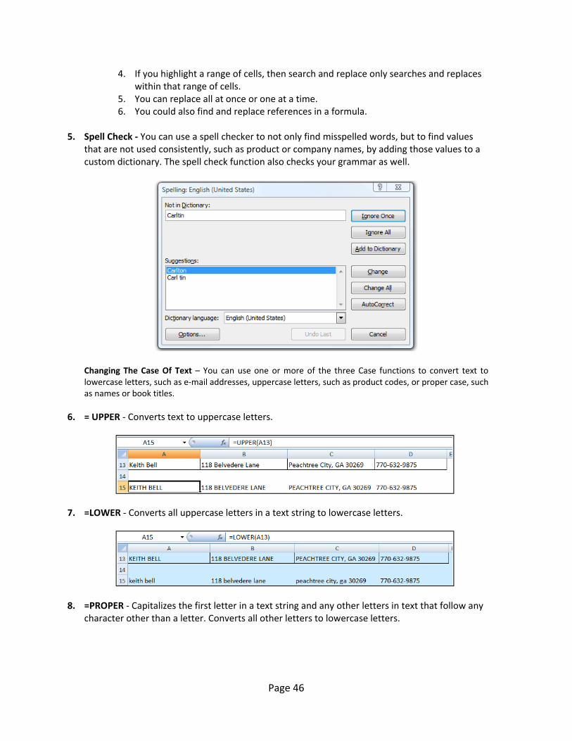
5. Spell Check ‐ You can use a spell checker to not only find misspelled words, but to find values
that are not used consistently, such as product or company names, by adding those values to a custom dictionary. The spell check function also checks your grammar as well.
Changing The Case Of Text – You can use one or more of the three Case functions to convert text to lowercase letters, such as e‐mail addresses, uppercase letters, such as product codes, or proper case, such as names or book titles.
6. = UPPER ‐ Converts text to uppercase letters.
7. =LOWER ‐ Converts all uppercase letters in a text string to lowercase letters.
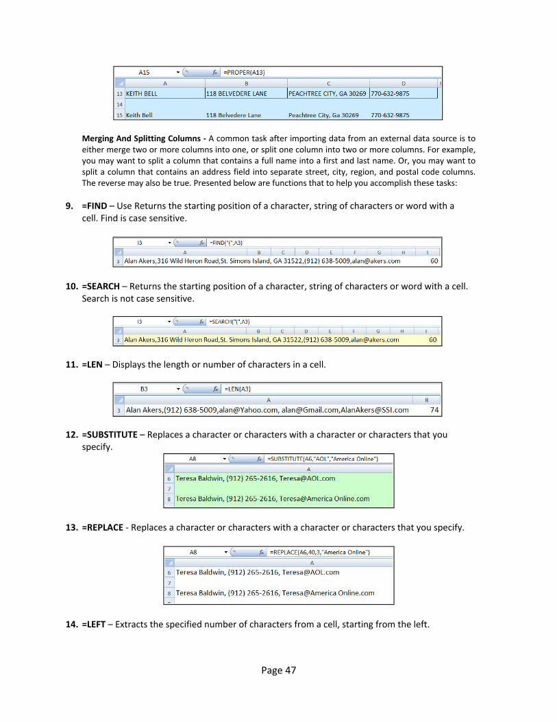
8. =PROPER ‐ Capitalizes the first letter in a text string and any other letters in text that follow any character other than a letter. Converts all other letters to lowercase letters.
Page 47
Merging And Splitting Columns ‐ A common task after importing data from an external data source is to either merge two or more columns into one, or split one column into two or more columns. For example, you may want to split a column that contains a full name into a first and last name. Or, you may want to split a column that contains an address field into separate street, city, region, and postal code columns. The reverse may also be true. Presented below are functions that to help you accomplish these tasks:
9. =FIND – Use Returns the starting position of a character, string of characters or word with a cell. Find is case sensitive.
10. =SEARCH – Returns the starting position of a character, string of characters or word with a cell. Search is not case sensitive.
11. =LEN – Displays the length or number of characters in a cell.
12. =SUBSTITUTE – Replaces a character or characters with a character or characters that you specify.
13. =REPLACE ‐ Replaces a character or characters with a character or characters that you specify.
14. =LEFT – Extracts the specified number of characters from a cell, starting from the left.

Page 48
15. =MID – Extracts the specified number of characters from a cell, starting from somewhere in the middle of the cell.
16. =RIGHT – Extracts the specified number of characters from a cell, starting from the right.
17. =Value – Converts text to values so the data can be added, subtracted, multiplied, divided or referenced in a function.
18. =CONCATENATE ‐ Joins two or more text strings into one text string.
Variations of these functions that are used when working with foreign languages: =FINDB – Use this when working with foreign characters like these ( "," ) =SEARCHB – Use this when working with foreign characters like these ( "," ) =REPLACEB – Use this when working with foreign characters like these ( "," ) =LEFTB – Use this when working with foreign characters like these ( "," ) =RIGHTB – Use this when working with foreign characters like these ( "," ) =LENB – Use this when working with foreign characters like these ( "," ) =MIDB – Use this when working with foreign characters like these ( "," )
Cleaning Text – (Removing Spaces And Nonprinting Characters From Text) ‐ Sometimes text values contain leading, trailing, or multiple embedded space characters (Unicode character set values 32 and 160), or nonprinting characters (Unicode character set values 0 to 31, 127, 129, 141, 143, 144, and 157). These characters can sometimes cause unexpected results when you sort, filter, or search. For example, in the external data source, users may make typographical errors by inadvertently adding extra space characters, or imported text data from external sources may contain nonprinting characters that are
Page 49
embedded in the text. Because these characters are not easily noticed, the unexpected results may be difficult to understand. Following is a list of functions you can use to remove these unwanted characters:
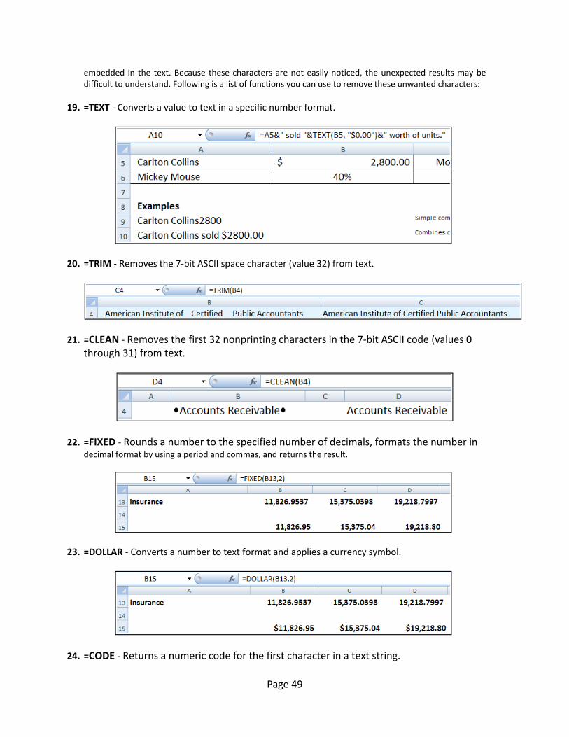
19. =TEXT ‐ Converts a value to text in a specific number format.
20. =TRIM ‐ Removes the 7‐bit ASCII space character (value 32) from text.
21. =CLEAN ‐ Removes the first 32 nonprinting characters in the 7‐bit ASCII code (values 0 through 31) from text.
22. =FIXED ‐ Rounds a number to the specified number of decimals, formats the number in decimal format by using a period and commas, and returns the result.
23. =DOLLAR ‐ Converts a number to text format and applies a currency symbol.
24. =CODE ‐ Returns a numeric code for the first character in a text string.
Page 50
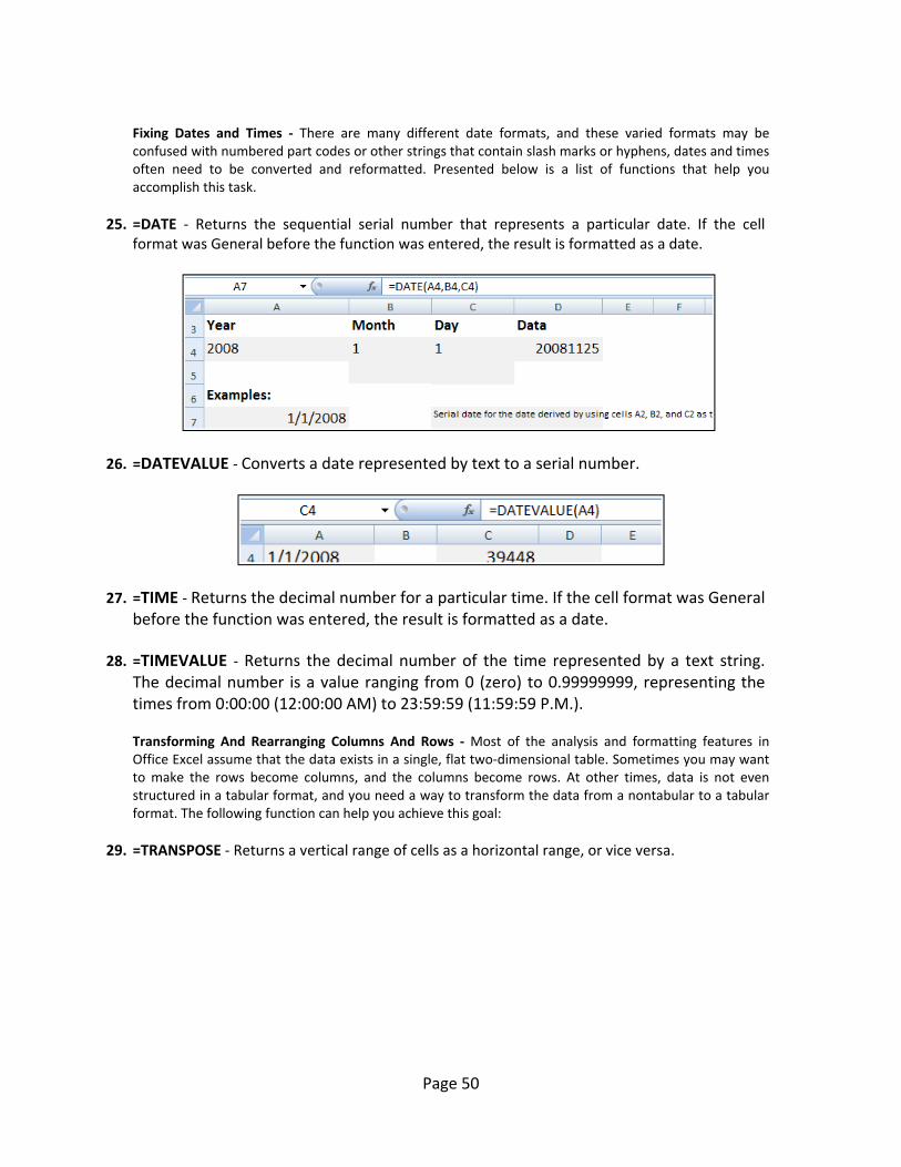
Fixing Dates and Times ‐ There are many different date formats, and these varied formats may be confused with numbered part codes or other strings that contain slash marks or hyphens, dates and times often need to be converted and reformatted. Presented below is a list of functions that help you accomplish this task.
25. =DATE ‐ Returns the sequential serial number that represents a particular date. If the cell format was General before the function was entered, the result is formatted as a date.
26. =DATEVALUE ‐ Converts a date represented by text to a serial number.
27. =TIME ‐ Returns the decimal number for a particular time. If the cell format was General before the function was entered, the result is formatted as a date.
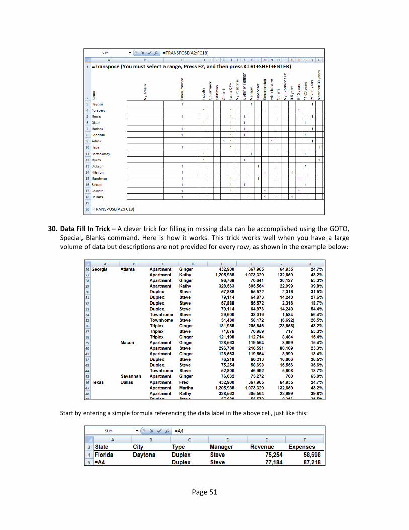
28. =TIMEVALUE ‐ Returns the decimal number of the time represented by a text string. The decimal number is a value ranging from 0 (zero) to 0.99999999, representing the times from 0:00:00 (12:00:00 AM) to 23:59:59 (11:59:59 P.M.). Transforming And Rearranging Columns And Rows ‐ Most of the analysis and formatting features in Office Excel assume that the data exists in a single, flat two‐dimensional table. Sometimes you may want to make the rows become columns, and the columns become rows. At other times, data is not even structured in a tabular format, and you need a way to transform the data from a nontabular to a tabular format. The following function can help you achieve this goal:
29. =TRANSPOSE ‐ Returns a vertical range of cells as a horizontal range, or vice versa.
Page 51
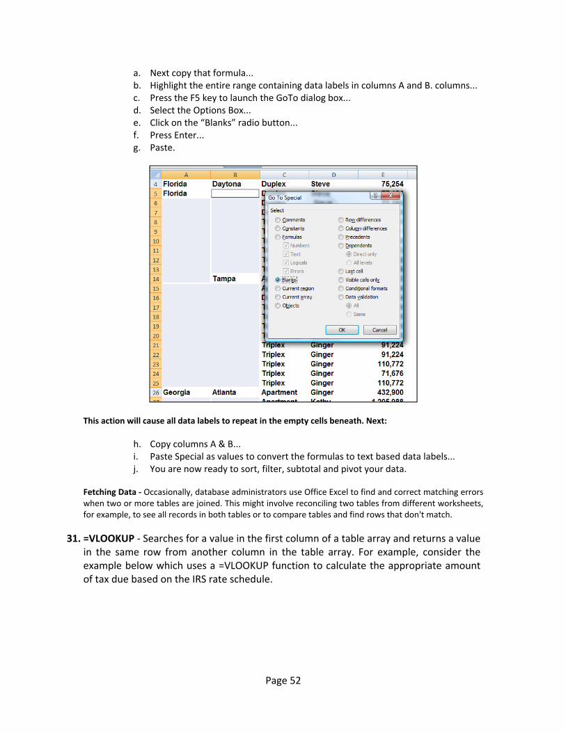
30. Data Fill In Trick – A clever trick for filling in missing data can be accomplished using the GOTO, Special, Blanks command. Here is how it works. This trick works well when you have a large volume of data but descriptions are not provided for every row, as shown in the example below:
Start by entering a simple formula referencing the data label in the above cell, just like this:
Page 52
a. Next copy that formula... b. Highlight the entire range containing data labels in columns A and B. columns... c. Press the F5 key to launch the GoTo dialog box... d. Select the Options Box... e. Click on the “Blanks” radio button... f. Press Enter... g. Paste.
This action will cause all data labels to repeat in the empty cells beneath. Next:
h. Copy columns A & B... i. Paste Special as values to convert the formulas to text based data labels... j. You are now ready to sort, filter, subtotal and pivot your data.
Fetching Data ‐ Occasionally, database administrators use Office Excel to find and correct matching errors when two or more tables are joined. This might involve reconciling two tables from different worksheets, for example, to see all records in both tables or to compare tables and find rows that don't match.
31. =VLOOKUP ‐ Searches for a value in the first column of a table array and returns a value in the same row from another column in the table array. For example, consider the example below which uses a =VLOOKUP function to calculate the appropriate amount of tax due based on the IRS rate schedule.

Page 53
As the Income statement shown in the shaded area is updated , the resulting taxable income amount is referenced in Cell F13. Next, 3 VLOOKUP functions pull the appropriate rate, base and threshold information from the rate schedule to be used in calculating income tax. Once calculated, the resulting tax is referenced back to the income statement for the purposes of computing Net income After taxes. Key points to Consider when Using VLOOKUP:
a. If you are looking up based on text, the first column containing lookup values must be sorted alphabetically in descending order – else it will not work properly.
b. If you are looking up based on text, you must have an exact match between the lookup value and the table array value.
c. If you are looking up based on values, the first column containing lookup
values must be sorted numerically in descending order – else it will not work properly.
d. If you are looking up based on values, then Excel will choose the closest value without going over. For example, if the lookup value is 198,000 and the table array contains values of 100,000 and 200,000, the n excel will choose 100,000 because 200,000 goes over or exceeds 198,000. (It might be helpful to think back to the old Bob barker game show the Price is Right.)

Page 54
32. =HLOOKUP ‐ Searches for a value in the top row of a table or an array of values, and then returns a value in the same column from a row you specify in the table or array.
33. =INDEX ‐ Returns a value or the reference to a value from within a table or range. There are two forms of the INDEX function: the array form and the reference form.
34. =MATCH ‐ Returns the relative position of an item in an array that matches a specified value in a specified order. Use MATCH instead of one of the LOOKUP functions when you need the position of an item in a range instead of the item itself.
35. =OFFSET ‐ Returns a reference to a range that is a specified number of rows and columns from a cell or range of cells. The reference that is returned can be a single cell or a range of cells. You can specify the number of rows and the number of columns to be returned.
36. Data Cleaning with Macros ‐ To periodically clean the same data source, consider recording a macro or writing code to automate the entire process. There are also a number of external add‐ins written by third‐party vendors, listed in the Third‐party providers section, that you can consider using if you don't have the time or resources to automate the process on your own.
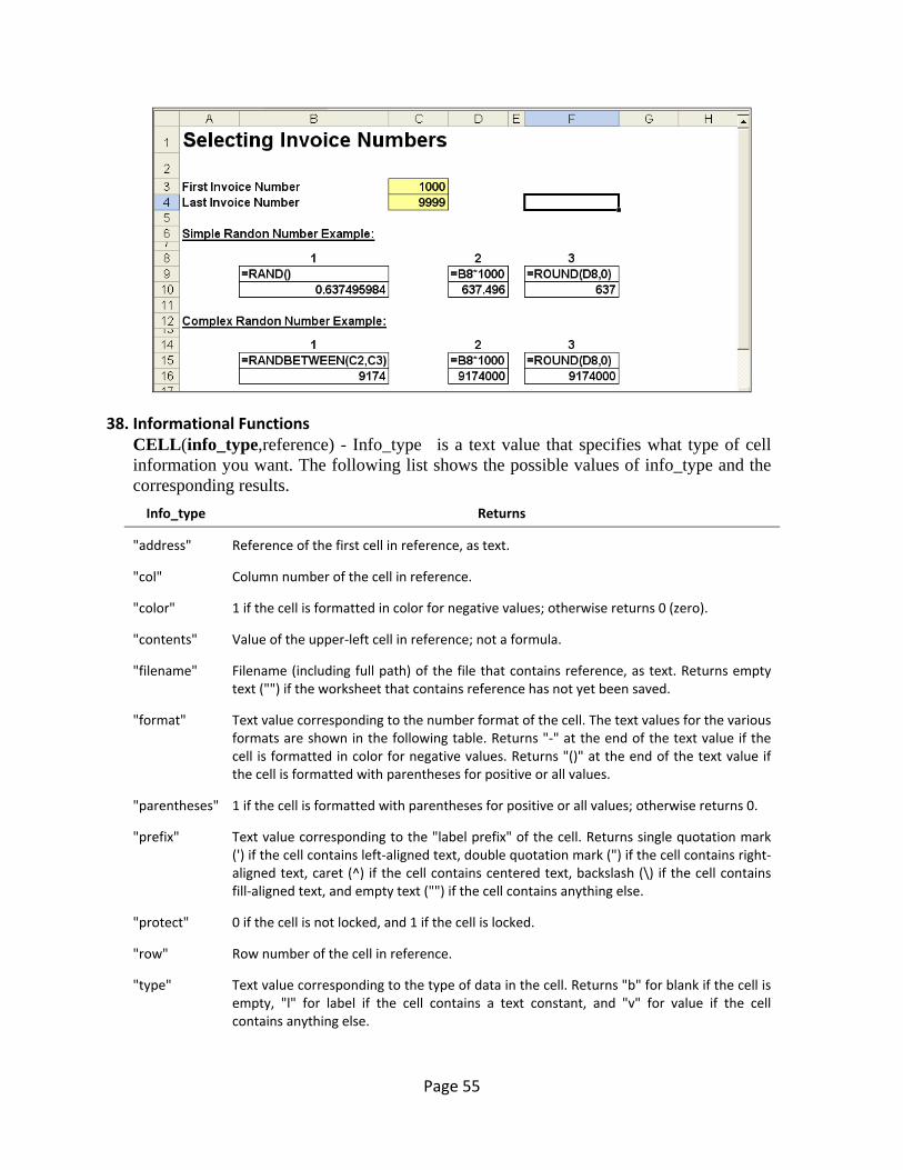
37. RAND( ), RANDBETWEEN( ), ROUND( ) – In Excel 2003, RANDBETWEEN is not in the standard EXCEL installation but if the analysis tool pack is installed and the add‐in activated it is an extremely useful function.
Page 55
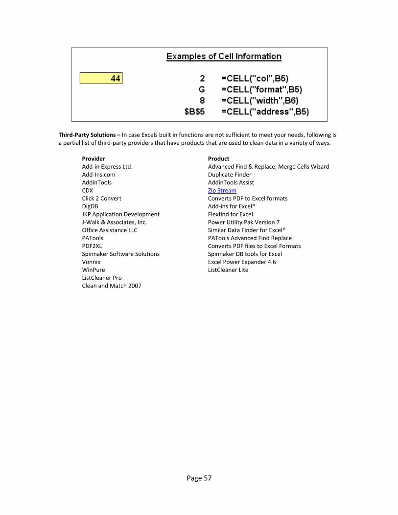
38. Informational Functions CELL(info_type,reference) - Info_type is a text value that specifies what type of cell information you want. The following list shows the possible values of info_type and the corresponding results. Info_type Returns
"address" Reference of the first cell in reference, as text.
"col" Column number of the cell in reference.
"color" 1 if the cell is formatted in color for negative values; otherwise returns 0 (zero).
"contents" Value of the upper‐left cell in reference; not a formula.
"filename" Filename (including full path) of the file that contains reference, as text. Returns empty text ("") if the worksheet that contains reference has not yet been saved.
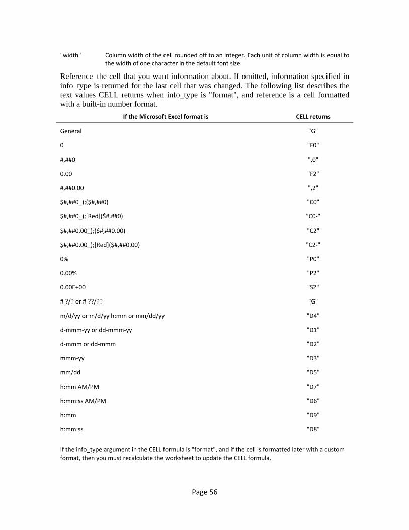
"format" Text value corresponding to the number format of the cell. The text values for the various formats are shown in the following table. Returns "‐" at the end of the text value if the cell is formatted in color for negative values. Returns "()" at the end of the text value if the cell is formatted with parentheses for positive or all values.
"parentheses" 1 if the cell is formatted with parentheses for positive or all values; otherwise returns 0.
"prefix" Text value corresponding to the "label prefix" of the cell. Returns single quotation mark (') if the cell contains left‐aligned text, double quotation mark (") if the cell contains right‐aligned text, caret (^) if the cell contains centered text, backslash (\) if the cell contains fill‐aligned text, and empty text ("") if the cell contains anything else.
"protect" 0 if the cell is not locked, and 1 if the cell is locked.
"row" Row number of the cell in reference.
"type" Text value corresponding to the type of data in the cell. Returns "b" for blank if the cell is empty, "l" for label if the cell contains a text constant, and "v" for value if the cell contains anything else.
Page 56
"width" Column width of the cell rounded off to an integer. Each unit of column width is equal to the width of one character in the default font size.
Reference the cell that you want information about. If omitted, information specified in info_type is returned for the last cell that was changed. The following list describes the text values CELL returns when info_type is "format", and reference is a cell formatted with a built-in number format.
If the Microsoft Excel format is CELL returns
General "G"
0 "F0"
#,##0 ",0"
0.00 "F2"
#,##0.00 ",2"
$#,##0_);($#,##0) "C0"
$#,##0_);[Red]($#,##0) "C0‐"
$#,##0.00_);($#,##0.00) "C2"
$#,##0.00_);[Red]($#,##0.00) "C2‐"
0% "P0"
0.00% "P2"
0.00E+00 "S2"
# ?/? or # ??/?? "G"
m/d/yy or m/d/yy h:mm or mm/dd/yy "D4"
d‐mmm‐yy or dd‐mmm‐yy "D1"
d‐mmm or dd‐mmm "D2"
mmm‐yy "D3"
mm/dd "D5"
h:mm AM/PM "D7"
h:mm:ss AM/PM "D6"
h:mm "D9"
h:mm:ss "D8"
If the info_type argument in the CELL formula is "format", and if the cell is formatted later with a custom format, then you must recalculate the worksheet to update the CELL formula.
Page 57
Third‐Party Solutions – In case Excels built in functions are not sufficient to meet your needs, following is a partial list of third‐party providers that have products that are used to clean data in a variety of ways.
Provider Product Add‐in Express Ltd. Advanced Find & Replace, Merge Cells Wizard Add‐Ins.com Duplicate Finder AddinTools AddinTools Assist CDX Zip Stream Click 2 Convert Converts PDF to Excel formats DigDB Add‐ins for Excel® JKP Application Development Flexfind for Excel J‐Walk & Associates, Inc. Power Utility Pak Version 7 Office Assistance LLC Similar Data Finder for Excel® PATools PATools Advanced Find Replace PDF2XL Converts PDF files to Excel Formats Spinnaker Software Solutions Spinnaker DB tools for Excel Vonnix Excel Power Expander 4.6 WinPure ListCleaner Lite ListCleaner Pro Clean and Match 2007
Page 58
Chapter 6
Data Commands
Page 59
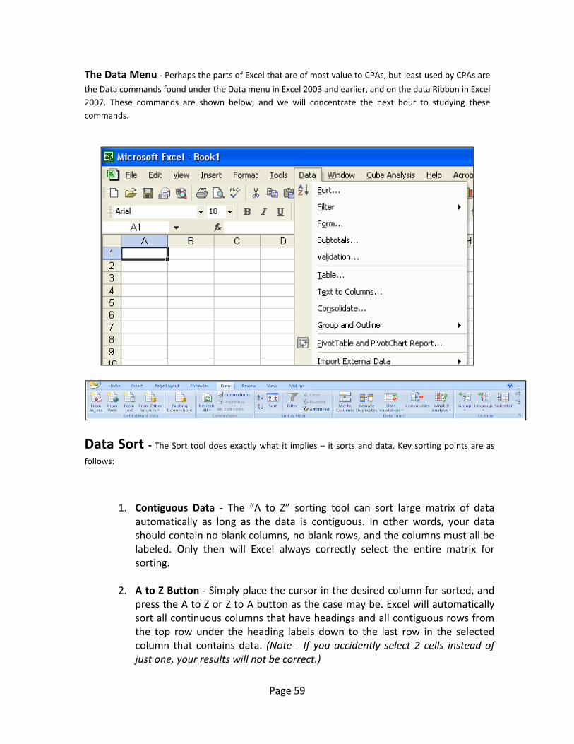
The Data Menu ‐ Perhaps the parts of Excel that are of most value to CPAs, but least used by CPAs are
the Data commands found under the Data menu in Excel 2003 and earlier, and on the data Ribbon in Excel 2007. These commands are shown below, and we will concentrate the next hour to studying these commands.
Data Sort ‐ The Sort tool does exactly what it implies – it sorts and data. Key sorting points are as
follows:
1. Contiguous Data ‐ The “A to Z” sorting tool can sort large matrix of data automatically as long as the data is contiguous. In other words, your data should contain no blank columns, no blank rows, and the columns must all be labeled. Only then will Excel always correctly select the entire matrix for sorting.
2. A to Z Button ‐ Simply place the cursor in the desired column for sorted, and press the A to Z or Z to A button as the case may be. Excel will automatically sort all continuous columns that have headings and all contiguous rows from the top row under the heading labels down to the last row in the selected column that contains data. (Note ‐ If you accidently select 2 cells instead of just one, your results will not be correct.)
Page 60
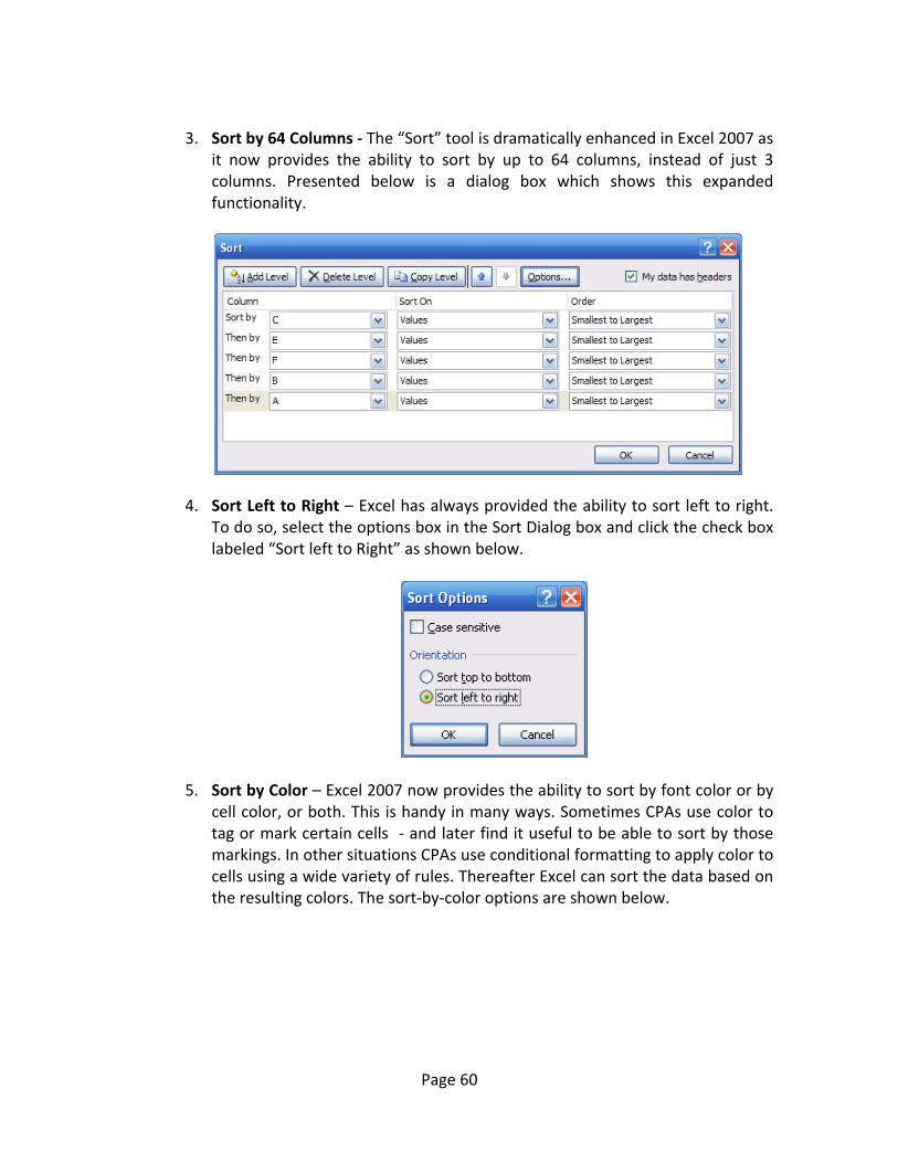
3. Sort by 64 Columns ‐ The “Sort” tool is dramatically enhanced in Excel 2007 as
it now provides the ability to sort by up to 64 columns, instead of just 3 columns. Presented below is a dialog box which shows this expanded functionality.
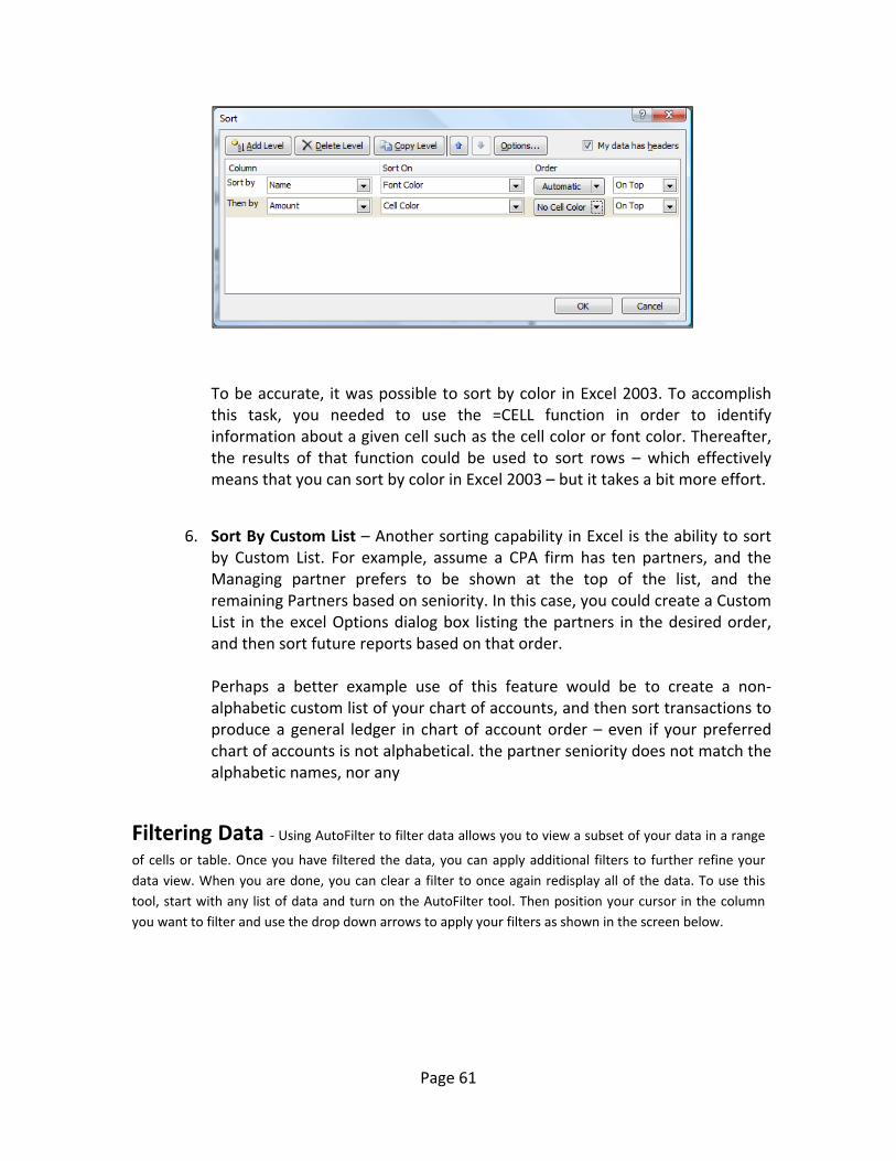
4. Sort Left to Right – Excel has always provided the ability to sort left to right.
To do so, select the options box in the Sort Dialog box and click the check box labeled “Sort left to Right” as shown below.
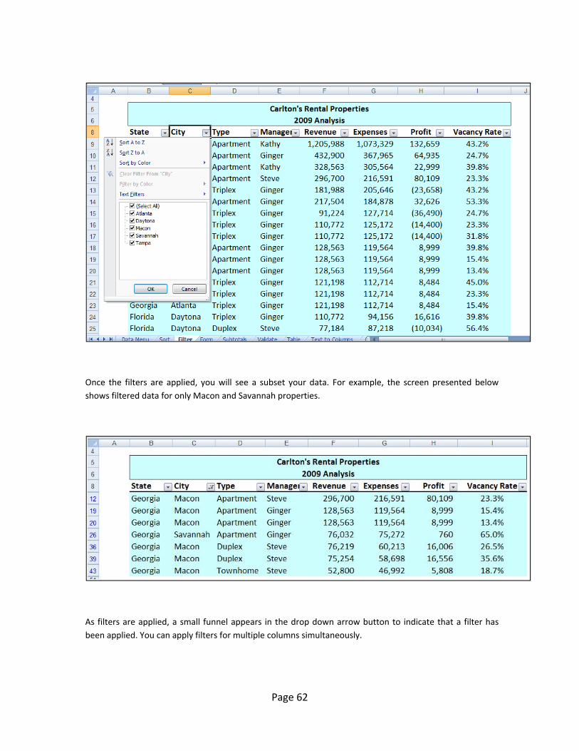
5. Sort by Color – Excel 2007 now provides the ability to sort by font color or by cell color, or both. This is handy in many ways. Sometimes CPAs use color to tag or mark certain cells ‐ and later find it useful to be able to sort by those markings. In other situations CPAs use conditional formatting to apply color to cells using a wide variety of rules. Thereafter Excel can sort the data based on the resulting colors. The sort‐by‐color options are shown below.
Page 61
To be accurate, it was possible to sort by color in Excel 2003. To accomplish this task, you needed to use the =CELL function in order to identify information about a given cell such as the cell color or font color. Thereafter, the results of that function could be used to sort rows – which effectively means that you can sort by color in Excel 2003 – but it takes a bit more effort.
6. Sort By Custom List – Another sorting capability in Excel is the ability to sort by Custom List. For example, assume a CPA firm has ten partners, and the Managing partner prefers to be shown at the top of the list, and the remaining Partners based on seniority. In this case, you could create a Custom List in the excel Options dialog box listing the partners in the desired order, and then sort future reports based on that order. Perhaps a better example use of this feature would be to create a non‐alphabetic custom list of your chart of accounts, and then sort transactions to produce a general ledger in chart of account order – even if your preferred chart of accounts is not alphabetical. the partner seniority does not match the alphabetic names, nor any
Filtering Data ‐ Using AutoFilter to filter data allows you to view a subset of your data in a range of cells or table. Once you have filtered the data, you can apply additional filters to further refine your data view. When you are done, you can clear a filter to once again redisplay all of the data. To use this tool, start with any list of data and turn on the AutoFilter tool. Then position your cursor in the column you want to filter and use the drop down arrows to apply your filters as shown in the screen below.
Page 62
Once the filters are applied, you will see a subset your data. For example, the screen presented below shows filtered data for only Macon and Savannah properties.
As filters are applied, a small funnel appears in the drop down arrow button to indicate that a filter has been applied. You can apply filters for multiple columns simultaneously.

Page 63
Key Points Concerning The AutoFilter Command:
1. Contiguous Data – The AutoFilter tools works best when you are working with data that is contiguous. In other words, your data should contain no blank columns, no blank rows, and the columns must all be labeled.
2. Filter by Multiple Columns ‐ You can filter by more than one column.
3. Removing Filters – In Excel 2003 and earlier, a faster way to remove multiple filters is to turn off filtering and then turn filtering back on. In Excel 2007 you can simple click the Clear button in the Sort and Filter Group as shown below.
4. Filters are Additive ‐ Each additional filter is based on the current filter and further reduces the subset of data.
5. Three Types of Filters – You can filter based on list values, by formats, or by criteria. Each of these filter types is mutually exclusive for each range of cells or column table. For example, you can filter by cell color or by a list of numbers, but not by both; you can filter by icon or by a custom filter, but not by both.
6. Filters Enabled ‐ A drop‐down arrow means that filtering is enabled but not
applied.
7. Filter Applied ‐ A Filter button means that a filter is applied.
Page 64
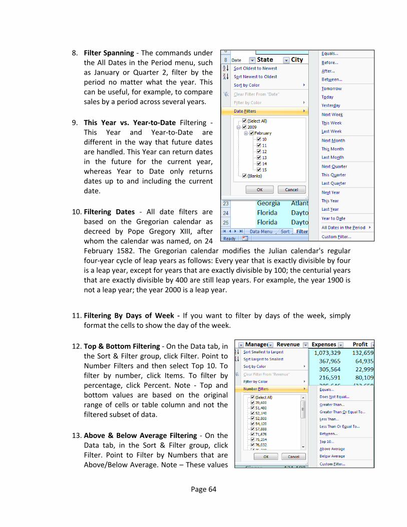
8. Filter Spanning ‐ The commands under the All Dates in the Period menu, such as January or Quarter 2, filter by the period no matter what the year. This can be useful, for example, to compare sales by a period across several years.
9. This Year vs. Year‐to‐Date Filtering ‐ This Year and Year‐to‐Date are different in the way that future dates are handled. This Year can return dates in the future for the current year, whereas Year to Date only returns dates up to and including the current date.
10. Filtering Dates ‐ All date filters are based on the Gregorian calendar as decreed by Pope Gregory XIII, after whom the calendar was named, on 24 February 1582. The Gregorian calendar modifies the Julian calendar's regular four‐year cycle of leap years as follows: Every year that is exactly divisible by four is a leap year, except for years that are exactly divisible by 100; the centurial years that are exactly divisible by 400 are still leap years. For example, the year 1900 is not a leap year; the year 2000 is a leap year.
11. Filtering By Days of Week ‐ If you want to filter by days of the week, simply format the cells to show the day of the week.
12. Top & Bottom Filtering ‐ On the Data tab, in the Sort & Filter group, click Filter. Point to Number Filters and then select Top 10. To filter by number, click Items. To filter by percentage, click Percent. Note ‐ Top and bottom values are based on the original range of cells or table column and not the filtered subset of data.
13. Above & Below Average Filtering ‐ On the Data tab, in the Sort & Filter group, click Filter. Point to Filter by Numbers that are Above/Below Average. Note – These values

Page 65
are based on the original range of cells or table column and not the filtered subset of data.
14. Filtering Out Blanks ‐ To filter for blanks, in the AutoFilter menu at the top of the list of values, clear (Select All), and then at the bottom of the list of values, select (Blanks).
15. Filtering By Color ‐ Select Filter by Color, and then depending on the type of format, select Filter by Cell Color, Filter by Font Color, or Filter by Cell Icon.
16. Filter by Selection ‐ To filter by text, number, or date or time, click Filter by Selected Cell's Value and then: To filter by cell color, click Filter by Selected Cell's Color. To filter by font color, click Filter by Selected Cell's Font Color. To filter by icon, click Filter by Selected Cell's Icon.
17. Refreshing Filters ‐ To reapply a filter after the data changes, click a cell in the range or table, and then on the Data tab, in the Sort & Filter group, click Reapply.
Data Form – Excel’s 2003 Data Form tool makes Excel look more and behave more like a database, such as Microsoft Access. (The Form button has not been included on the Office Fluent user interface Ribbon, but you can still use it in Office Excel 2007 by adding the Form button to the Quick Access Toolbar.)
A data form provides a convenient means to enter or display one complete row of information in a range or table without scrolling horizontally. You may find that using a data form can make data entry easier than moving from column to column when you
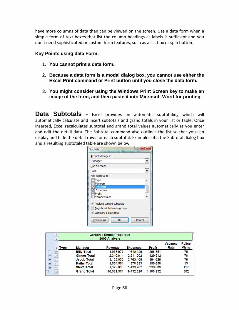
Page 66
have more columns of data than can be viewed on the screen. Use a data form when a simple form of text boxes that list the column headings as labels is sufficient and you don't need sophisticated or custom form features, such as a list box or spin button. Key Points using data Form:
1. You cannot print a data form. 2. Because a data form is a modal dialog box, you cannot use either the
Excel Print command or Print button until you close the data form. 3. You might consider using the Windows Print Screen key to make an
image of the form, and then paste it into Microsoft Word for printing. Data Subtotals – Excel provides an automatic subtotaling which will automatically calculate and insert subtotals and grand totals in your list or table. Once inserted, Excel recalculates subtotal and grand total values automatically as you enter and edit the detail data. The Subtotal command also outlines the list so that you can display and hide the detail rows for each subtotal. Examples of a the Subtotal dialog box and a resulting subtotaled table are shown below.
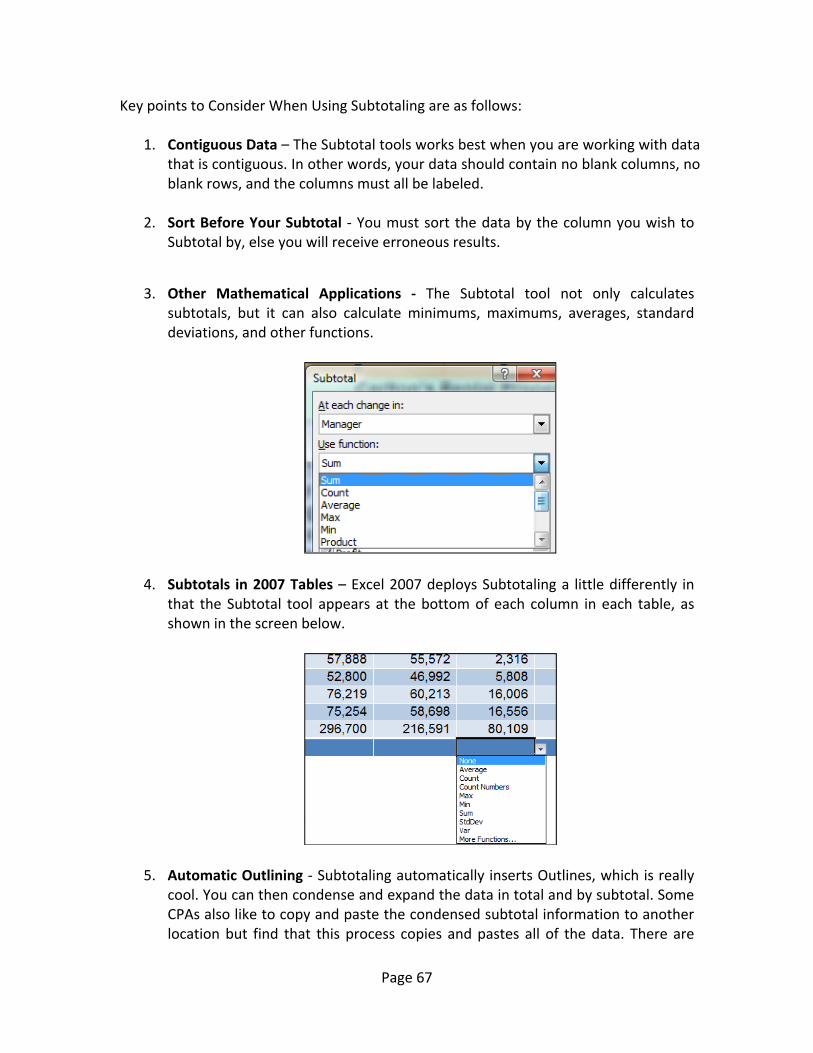
Page 67
Key points to Consider When Using Subtotaling are as follows:
1. Contiguous Data – The Subtotal tools works best when you are working with data that is contiguous. In other words, your data should contain no blank columns, no blank rows, and the columns must all be labeled.
2. Sort Before Your Subtotal ‐ You must sort the data by the column you wish to Subtotal by, else you will receive erroneous results.
3. Other Mathematical Applications ‐ The Subtotal tool not only calculates subtotals, but it can also calculate minimums, maximums, averages, standard deviations, and other functions.
4. Subtotals in 2007 Tables – Excel 2007 deploys Subtotaling a little differently in that the Subtotal tool appears at the bottom of each column in each table, as shown in the screen below.
5. Automatic Outlining ‐ Subtotaling automatically inserts Outlines, which is really cool. You can then condense and expand the data in total and by subtotal. Some CPAs also like to copy and paste the condensed subtotal information to another location but find that this process copies and pastes all of the data. There are
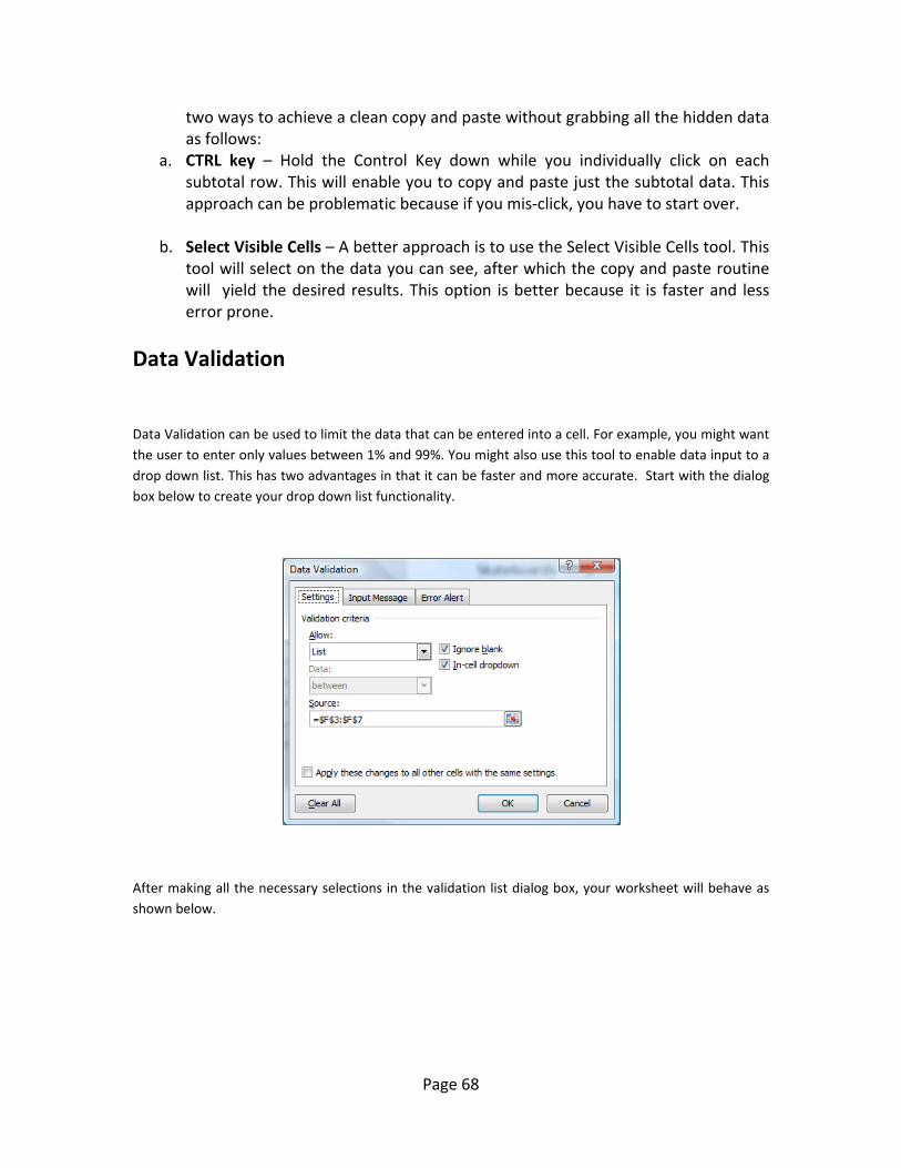
Page 68
two ways to achieve a clean copy and paste without grabbing all the hidden data as follows:
a. CTRL key – Hold the Control Key down while you individually click on each subtotal row. This will enable you to copy and paste just the subtotal data. This approach can be problematic because if you mis‐click, you have to start over.
b. Select Visible Cells – A better approach is to use the Select Visible Cells tool. This
tool will select on the data you can see, after which the copy and paste routine will yield the desired results. This option is better because it is faster and less error prone.
Data Validation
Data Validation can be used to limit the data that can be entered into a cell. For example, you might want the user to enter only values between 1% and 99%. You might also use this tool to enable data input to a drop down list. This has two advantages in that it can be faster and more accurate. Start with the dialog box below to create your drop down list functionality.
After making all the necessary selections in the validation list dialog box, your worksheet will behave as shown below.
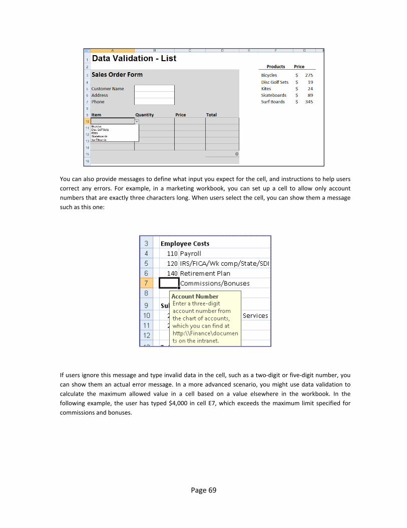
Page 69
You can also provide messages to define what input you expect for the cell, and instructions to help users correct any errors. For example, in a marketing workbook, you can set up a cell to allow only account numbers that are exactly three characters long. When users select the cell, you can show them a message such as this one:
If users ignore this message and type invalid data in the cell, such as a two‐digit or five‐digit number, you can show them an actual error message. In a more advanced scenario, you might use data validation to calculate the maximum allowed value in a cell based on a value elsewhere in the workbook. In the following example, the user has typed $4,000 in cell E7, which exceeds the maximum limit specified for commissions and bonuses.

Page 70
If the payroll budget were to increase or decrease, the allowed maximum in E7 would automatically increase or decrease with it.
PivotTables
The PivotTable report tool provides an interactive way to summarize large amounts of data. Use should use the PivotTable tools to crunch and analyze numerical data PivotTable reports are particularly useful in the following situations:
a. Rearranging rows to columns or columns to rows (or "pivoting") to see different summaries of the source data.
b. Filtering, sorting, grouping, and conditionally formatting your data. c. Preparing concise, attractive, and annotated online or printed reports d. Querying large amounts of data. e. Subtotaling and aggregating numeric data. f. Summarizing data by categories and subcategories g. Creating custom calculations and formulas. h. Expanding and collapsing levels of data. i. Drilling down to details from the summary data
In essence, PivotTables present multidimensional data views to the user – this process is often referred to as “modeling”, “data‐cube analysis”, or “OLAP data cubes”. To re‐arrange the PivotTable data, just drag and drop column and row headings to move data around. PivotTables are a great data analysis tool for management.
If you have never used a PivotTable before, initially the concept can be difficult to grasp. The best way to understand a PivotTable is to create a blank Pivot Table and then drag
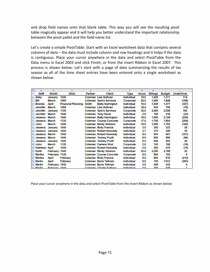
Page 71
and drop field names onto that blank table. This way you will see the resulting pivot table magically appear and it will help you better understand the important relationship between the pivot pallet and the field name list. Let’s create a simple PivotTable. Start with an Excel worksheet data that contains several columns of data – the data must include column and row headings and it helps if the data is contiguous. Place your cursor anywhere in the data and select PivotTable from the Data menu in Excel 2003 and click Finish; or from the insert Ribbon in Excel 2007. This process is shown below: Let’s start with a page of data summarizing the results of tax season as all of the time sheet entries have been entered onto a single worksheet as shown below.
Place your cursor anywhere in the data and select PivotTable from the Insert Ribbon as shown below:
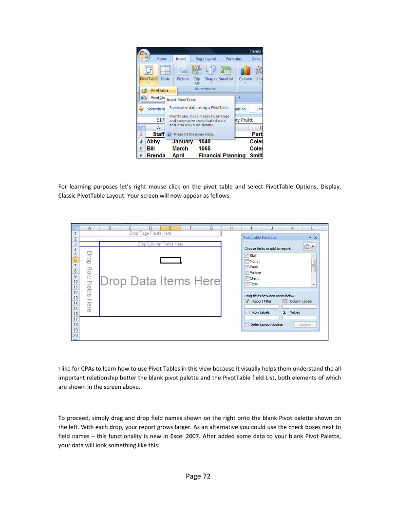
Page 72
For learning purposes let’s right mouse click on the pivot table and select PivotTable Options, Display, Classic PivotTable Layout. Your screen will now appear as follows:
I like for CPAs to learn how to use Pivot Tables in this view because it visually helps them understand the all important relationship better the blank pivot palette and the PivotTable field List, both elements of which are shown in the screen above.
To proceed, simply drag and drop field names shown on the right onto the blank Pivot palette shown on the left. With each drop, your report grows larger. As an alternative you could use the check boxes next to field names – this functionality is new in Excel 2007. After added some data to your blank Pivot Palette, your data will look something like this:

Page 73
Next format and filter the Pivot Report. Very quickly your report comes together as shown below. Notice the filter button has been applied and a Pivot table style has also been applied for appearance.
Double clicking on any number in a pivot report will automatically produce a new worksheet complete with all supporting detail that comprises the summary number.
There are a multitude of PivotTable options that can be applied to alter the appearance or behavior of your Pivot table.
Page 74
Key Points Concerning Pivot Tables are as Follows:
a. You can create as many Pivot Reports as you want from your initial raw data page. Your raw data remains unchanged as new Pivot tables are created.
b. As your raw data changes, your pivot tables are updated each time you press the refresh button. Or if you prefer you can set your PivotTables to update themselves at regularly scheduled intervals – say every ten minutes.
c. A key to understanding PivotTables is understanding the relationship between the Blank Pivot palette and the PivotTable Field list. As data is selected in the list, it appears on the Pivot table Report.
d. You can alter the PivotTable simple by dragging and dropping the field names in different locations on the Pivot palette, or in different locations in the PivotTable Field list Box.
e. PivotTables can be pivoted.
f. PivotTables can be sorted by any Column. (Or by any row when sorting left to right)
g. PivotTables can be Filtered.
h. PivotTables can be Drilled.
i. PivotTables can be copied and pasted.
j. PivotTables can be formatted using PivotTable Styles, as shown below.
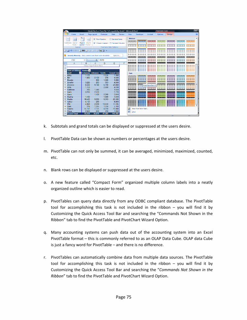
Page 75
k. Subtotals and grand totals can be displayed or suppressed at the users desire.
l. PivotTable Data can be shown as numbers or percentages at the users desire.
m. PivotTable can not only be summed, it can be averaged, minimized, maximized, counted, etc.
n. Blank rows can be displayed or suppressed at the users desire.
o. A new feature called “Compact Form” organized multiple column labels into a neatly organized outline which is easier to read.
p. PivotTables can query data directly from any ODBC compliant database. The PivotTable tool for accomplishing this task is not included in the ribbon – you will find it by Customizing the Quick Access Tool Bar and searching the “Commands Not Shown in the Ribbon” tab to find the PivotTable and PivotChart Wizard Option.
q. Many accounting systems can push data out of the accounting system into an Excel PivotTable format – this is commonly referred to as an OLAP Data Cube. OLAP data Cube is just a fancy word for PivotTable – and there is no difference.
r. PivotTables can automatically combine data from multiple data sources. The PivotTable tool for accomplishing this task is not included in the ribbon – you will find it by Customizing the Quick Access Tool Bar and searching the “Commands Not Shown in the Ribbon” tab to find the PivotTable and PivotChart Wizard Option.

Page 76
s. Excel also provides a PivotChart function which works similarly to PivotTables. Presented below is an example PivotChart.
Excel 2003 PivotTables work very similarly as shown below. Excel creates a blank PivotTable, and the user must drag and drop the various fields from the PivotTable Field List onto the appropriate column, row, or data section. As you drag and drop these items, the resulting report is displayed on the fly. Here is the blank Pivot Palette view.
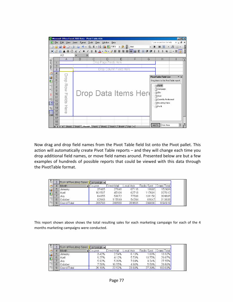
Page 77
Now drag and drop field names from the Pivot Table field list onto the Pivot pallet. This action will automatically create Pivot Table reports – and they will change each time you drop additional field names, or move field names around. Presented below are but a few examples of hundreds of possible reports that could be viewed with this data through the PivotTable format.
This report shown above shows the total resulting sales for each marketing campaign for each of the 4 months marketing campaigns were conducted.
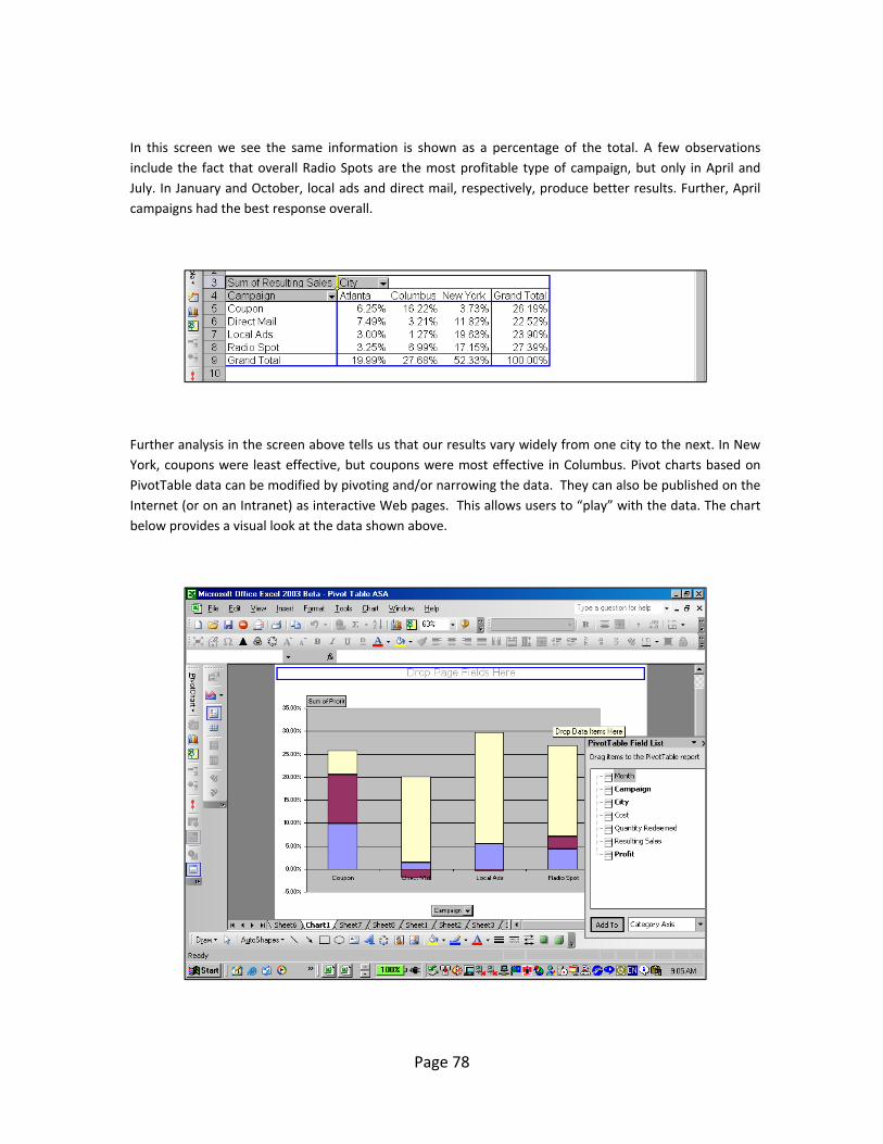
Page 78
In this screen we see the same information is shown as a percentage of the total. A few observations include the fact that overall Radio Spots are the most profitable type of campaign, but only in April and July. In January and October, local ads and direct mail, respectively, produce better results. Further, April campaigns had the best response overall.
Further analysis in the screen above tells us that our results vary widely from one city to the next. In New York, coupons were least effective, but coupons were most effective in Columbus. Pivot charts based on PivotTable data can be modified by pivoting and/or narrowing the data. They can also be published on the Internet (or on an Intranet) as interactive Web pages. This allows users to “play” with the data. The chart below provides a visual look at the data shown above.

Page 79
Filtering Pivot Tables ‐ If you take a close look at your resulting pivot tables, you will notice that Excel automatically inserts a filter button on each field list as shown by the drop down arrows in the screen below:
This drop down filter list makes it easy to refine your report to include just the data you want.
Drilling Pivot Tables ‐ Another nice feature in pivot tables is that they are automatically drillable. Simply double click on any number in a pivot report top have Excel automatically insert a new sheet and produce the detailed report underlying the number you clicked on. An example of this is shown below:
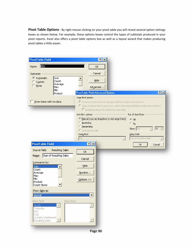
Page 80
Pivot Table Options ‐ By right mouse clicking on your pivot table you will reveal several option settings
boxes as shown below. For example, these options boxes control the types of subtotals produced in your pivot reports. Excel also offers a pivot table options box as well as a layout wizard that makes producing pivot tables a little easier.
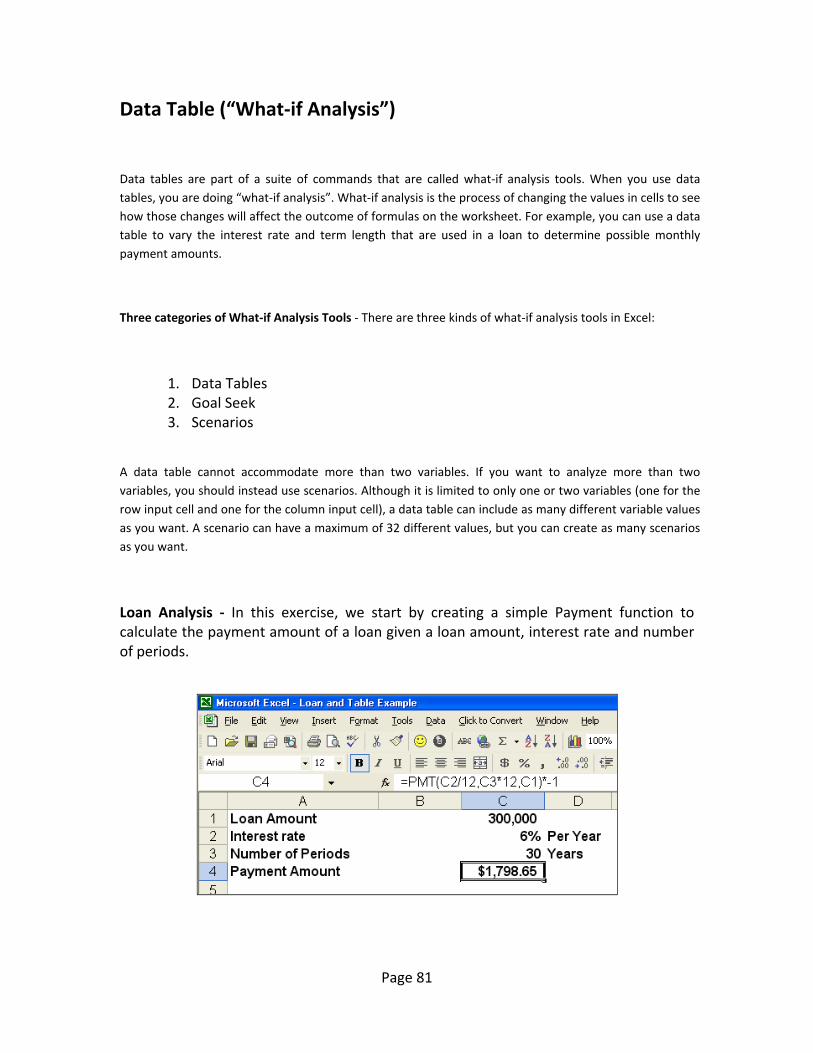
Page 81
Data Table (“What‐if Analysis”)
Data tables are part of a suite of commands that are called what‐if analysis tools. When you use data tables, you are doing “what‐if analysis”. What‐if analysis is the process of changing the values in cells to see how those changes will affect the outcome of formulas on the worksheet. For example, you can use a data table to vary the interest rate and term length that are used in a loan to determine possible monthly payment amounts.
Three categories of What‐if Analysis Tools ‐ There are three kinds of what‐if analysis tools in Excel:
1. Data Tables 2. Goal Seek 3. Scenarios
A data table cannot accommodate more than two variables. If you want to analyze more than two variables, you should instead use scenarios. Although it is limited to only one or two variables (one for the row input cell and one for the column input cell), a data table can include as many different variable values as you want. A scenario can have a maximum of 32 different values, but you can create as many scenarios as you want.
Loan Analysis ‐ In this exercise, we start by creating a simple Payment function to calculate the payment amount of a loan given a loan amount, interest rate and number of periods.
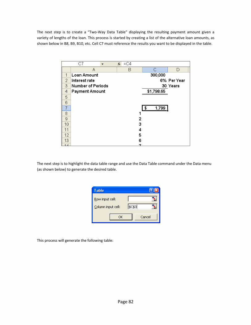
Page 82
The next step is to create a “Two‐Way Data Table” displaying the resulting payment amount given a variety of lengths of the loan. This process is started by creating a list of the alternative loan amounts, as shown below in B8, B9, B10, etc. Cell C7 must reference the results you want to be displayed in the table.
The next step is to highlight the data table range and use the Data Table command under the Data menu (as shown below) to generate the desired table.
This process will generate the following table:
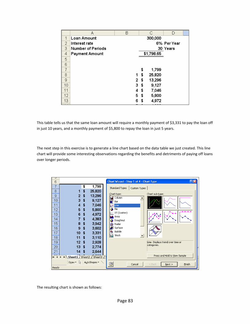
Page 83
This table tells us that the same loan amount will require a monthly payment of $3,331 to pay the loan off in just 10 years, and a monthly payment of $5,800 to repay the loan in just 5 years.
The next step in this exercise is to generate a line chart based on the data table we just created. This line chart will provide some interesting observations regarding the benefits and detriments of paying off loans over longer periods.
The resulting chart is shown as follows:
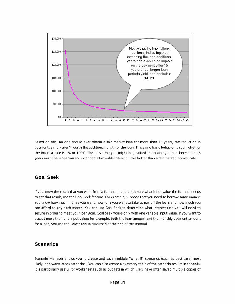
Page 84
Based on this, no one should ever obtain a fair market loan for more than 15 years, the reduction in payments simply aren’t worth the additional length of the loan. This same basic behavior is seen whether the interest rate is 1% or 100%. The only time you might be justified in obtaining a loan loner than 15 years might be when you are extended a favorable interest – this better than a fair market interest rate.
Goal Seek
If you know the result that you want from a formula, but are not sure what input value the formula needs to get that result, use the Goal Seek feature. For example, suppose that you need to borrow some money. You know how much money you want, how long you want to take to pay off the loan, and how much you can afford to pay each month. You can use Goal Seek to determine what interest rate you will need to secure in order to meet your loan goal. Goal Seek works only with one variable input value. If you want to accept more than one input value; for example, both the loan amount and the monthly payment amount for a loan, you use the Solver add‐in discussed at the end of this manual.
Scenarios
Scenario Manager allows you to create and save multiple “what if” scenarios (such as best case, most likely, and worst cases scenarios). You can also create a summary table of the scenario results in seconds. It is particularly useful for worksheets such as budgets in which users have often saved multiple copies of
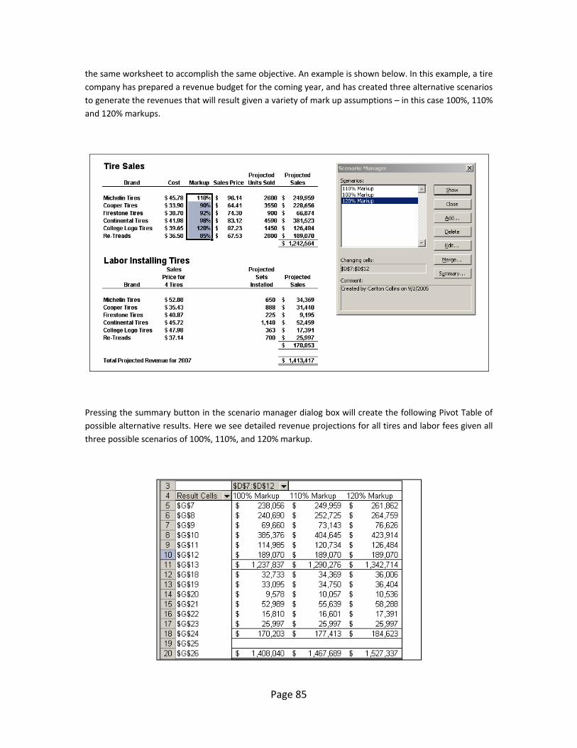
Page 85
the same worksheet to accomplish the same objective. An example is shown below. In this example, a tire company has prepared a revenue budget for the coming year, and has created three alternative scenarios to generate the revenues that will result given a variety of mark up assumptions – in this case 100%, 110% and 120% markups.
Pressing the summary button in the scenario manager dialog box will create the following Pivot Table of possible alternative results. Here we see detailed revenue projections for all tires and labor fees given all three possible scenarios of 100%, 110%, and 120% markup.
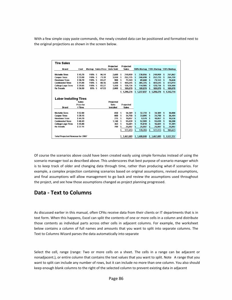
Page 86
With a few simple copy paste commands, the newly created data can be positioned and formatted next to the original projections as shown in the screen below.
Of course the scenarios above could have been created easily using simple formulas instead of using the scenario manager tool as described above. This underscores that best purpose of scenario manager which is to keep track of older and changing data through time, rather than producing what‐if scenarios. For example, a complex projection containing scenarios based on original assumptions, revised assumptions, and final assumptions will allow management to go back and review the assumptions used throughout the project, and see how those assumptions changed as project planning progressed.
Data ‐ Text to Columns
As discussed earlier in this manual, often CPAs receive data from their clients or IT departments that is in text form. When this happens, Excel can split the contents of one or more cells in a column and distribute those contents as individual parts across other cells in adjacent columns. For example, the worksheet below contains a column of full names and amounts that you want to split into separate columns. The Text to Columns Wizard parses the data automatically into separate
Select the cell, range (range: Two or more cells on a sheet. The cells in a range can be adjacent or nonadjacent.), or entire column that contains the text values that you want to split. Note A range that you want to split can include any number of rows, but it can include no more than one column. You also should keep enough blank columns to the right of the selected column to prevent existing data in adjacent
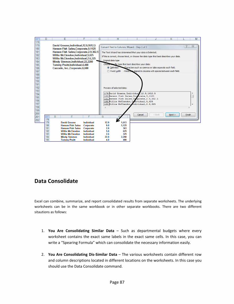
Page 87
Data Consolidate
Excel can combine, summarize, and report consolidated results from separate worksheets. The underlying worksheets can be in the same workbook or in other separate workbooks. There are two different sitautions as follows:
1. You Are Consolidating Similar Data – Such as departmental budgets where every worksheet contains the exact same labels in the exact same cells. In this case, you can write a “Spearing Formula” which can consolidate the necessary information easily.
2. You Are Consolidating Dis‐Similar Data – The various worksheets contain different row and column descriptions located in different locations on the worksheets. In this case you should use the Data Consolidate command.
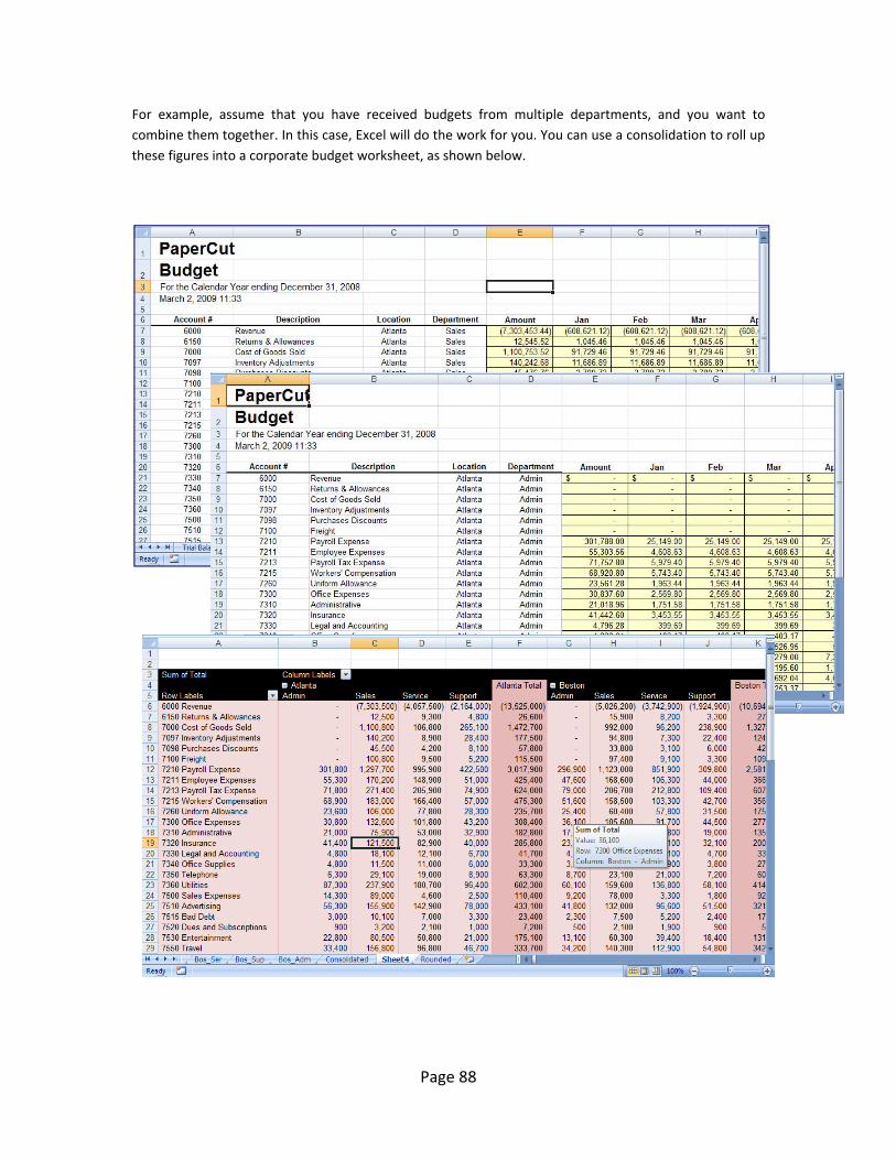
Page 88
For example, assume that you have received budgets from multiple departments, and you want to combine them together. In this case, Excel will do the work for you. You can use a consolidation to roll up these figures into a corporate budget worksheet, as shown below.
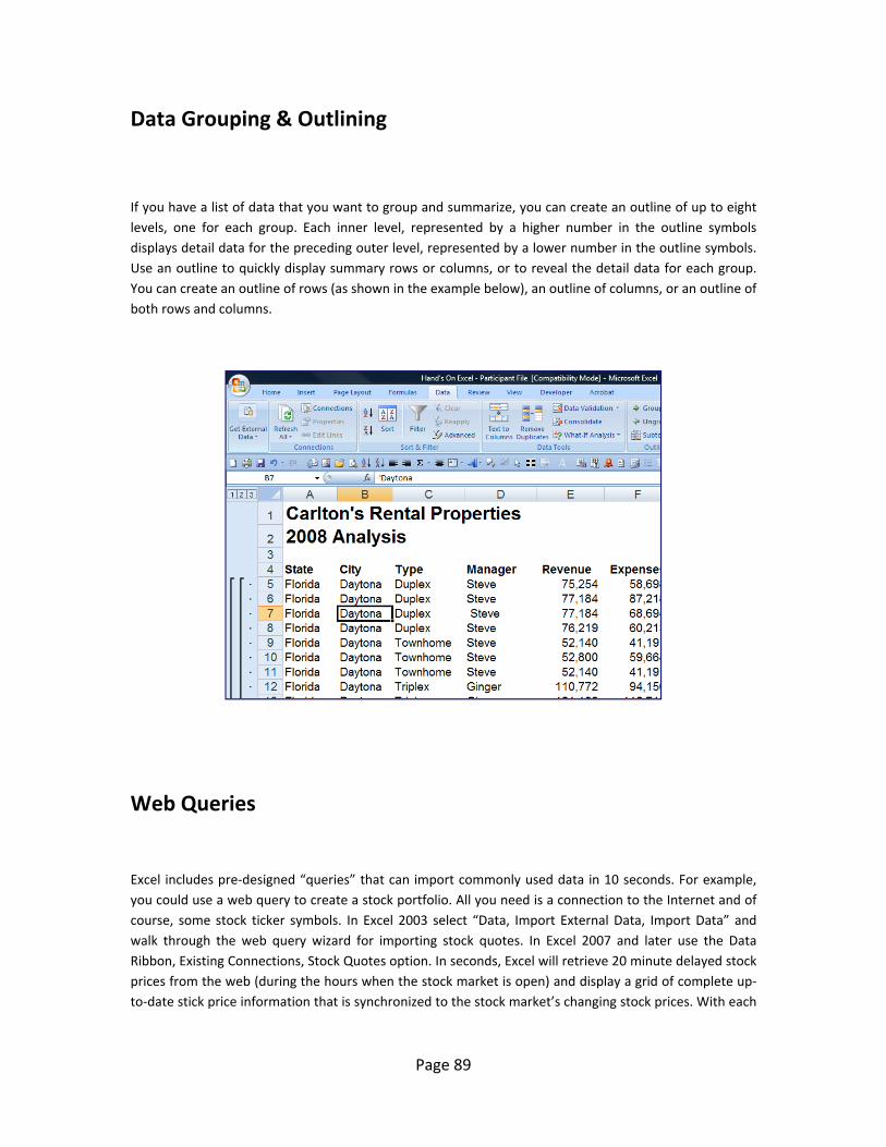
Page 89
Data Grouping & Outlining
If you have a list of data that you want to group and summarize, you can create an outline of up to eight levels, one for each group. Each inner level, represented by a higher number in the outline symbols displays detail data for the preceding outer level, represented by a lower number in the outline symbols. Use an outline to quickly display summary rows or columns, or to reveal the detail data for each group. You can create an outline of rows (as shown in the example below), an outline of columns, or an outline of both rows and columns.
Web Queries
Excel includes pre‐designed “queries” that can import commonly used data in 10 seconds. For example, you could use a web query to create a stock portfolio. All you need is a connection to the Internet and of course, some stock ticker symbols. In Excel 2003 select “Data, Import External Data, Import Data” and walk through the web query wizard for importing stock quotes. In Excel 2007 and later use the Data Ribbon, Existing Connections, Stock Quotes option. In seconds, Excel will retrieve 20 minute delayed stock prices from the web (during the hours when the stock market is open) and display a grid of complete up‐to‐date stick price information that is synchronized to the stock market’s changing stock prices. With each
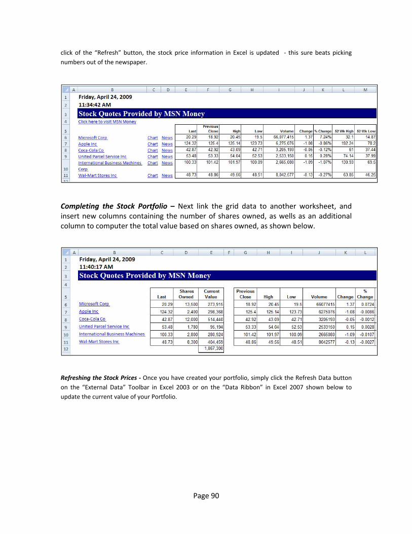
Page 90
click of the “Refresh” button, the stock price information in Excel is updated ‐ this sure beats picking numbers out of the newspaper.
Completing the Stock Portfolio – Next link the grid data to another worksheet, and insert new columns containing the number of shares owned, as wells as an additional column to computer the total value based on shares owned, as shown below.
Refreshing the Stock Prices ‐ Once you have created your portfolio, simply click the Refresh Data button on the “External Data” Toolbar in Excel 2003 or on the “Data Ribbon” in Excel 2007 shown below to update the current value of your Portfolio.
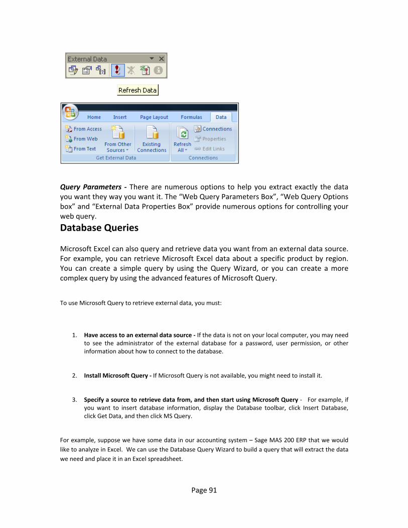
Page 91
Query Parameters ‐ There are numerous options to help you extract exactly the data you want they way you want it. The “Web Query Parameters Box”, “Web Query Options box” and “External Data Properties Box” provide numerous options for controlling your web query.
Database Queries Microsoft Excel can also query and retrieve data you want from an external data source. For example, you can retrieve Microsoft Excel data about a specific product by region. You can create a simple query by using the Query Wizard, or you can create a more complex query by using the advanced features of Microsoft Query.
To use Microsoft Query to retrieve external data, you must:
1. Have access to an external data source ‐ If the data is not on your local computer, you may need to see the administrator of the external database for a password, user permission, or other information about how to connect to the database.
2. Install Microsoft Query ‐ If Microsoft Query is not available, you might need to install it.
3. Specify a source to retrieve data from, and then start using Microsoft Query ‐ For example, if you want to insert database information, display the Database toolbar, click Insert Database, click Get Data, and then click MS Query.
For example, suppose we have some data in our accounting system – Sage MAS 200 ERP that we would like to analyze in Excel. We can use the Database Query Wizard to build a query that will extract the data we need and place it in an Excel spreadsheet.
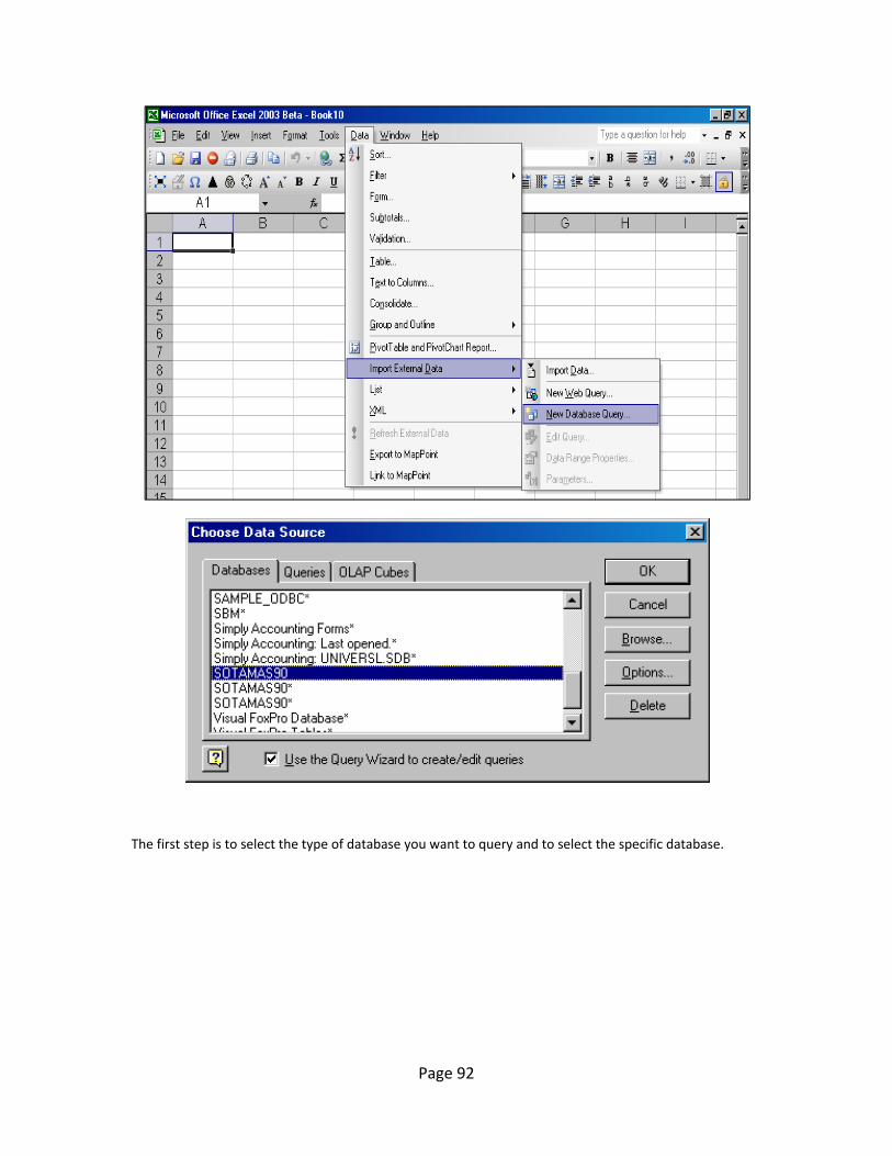
Page 92
The first step is to select the type of database you want to query and to select the specific database.
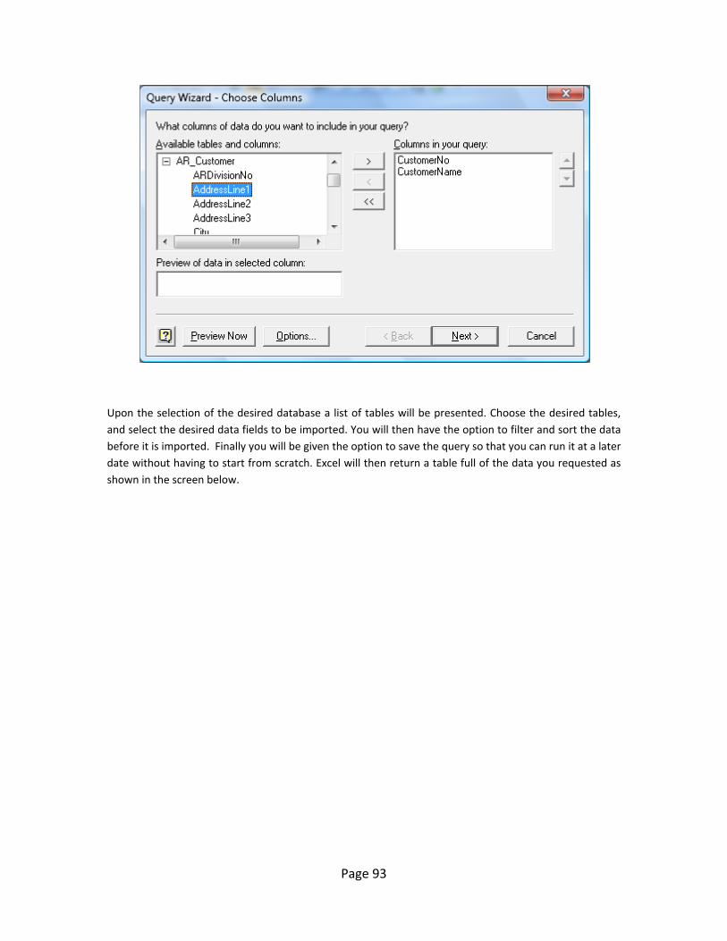
Page 93
Upon the selection of the desired database a list of tables will be presented. Choose the desired tables, and select the desired data fields to be imported. You will then have the option to filter and sort the data before it is imported. Finally you will be given the option to save the query so that you can run it at a later date without having to start from scratch. Excel will then return a table full of the data you requested as shown in the screen below.

Page 94

Page 95
Chapter 7
MACROS Automating Your Key Strokes

Page 96
Macros
Macros offer a powerful and flexible way to extend the features of Excel. They allow the automation of repetitive tasks such as printing, formatting, configuring, or otherwise manipulating data in Excel. In its’ simplest form, a macro is a recording of your keystrokes. While macros represent one of the stronger features found in Excel, they are rather easy to create and use. There are six major points that I like to make about macros as follows.
1. Record, Use Excel, Stop Recording – To create a macro, simply turn on the macro recorder, use Excel as you normally do, then turn off the recorder. Presto – you have created a macro. While the process is simple from the user’s point of view, underneath the covers Excel creates a Visual Basic subroutine using sophisticated Visual Basic programming commands.
2. Macro Location – Macros can be stored in either of two locations, as follows:
a. The workbook you are using, or b. Your Personal Macro Workbook (which by default is hidden from view)
If your macro applies to all workbooks, then store it in the Personal Macro Workbook so it will always be available in all of your Excel workbooks; otherwise store it in your current workbook. A macro stored in your current workbook will be embedded and included in the workbook, even if you e‐mail the workbook to another user.
3. Assign your Macro to an Icon, Text or a Button – To make it easy to run your macro, you should assign it to a toolbar icon so it will always be available no matter which workbooks you have open. If the macro applies only to your current workbook, then assign it to Text or a macro Button so it will be quickly available in your current workbook.
4. Absolute versus Relative Macros – An “Absolute” macro will always affect the same cells each time whereas a “Relative” macro will affect those cells relative to where your cursor is positioned when you invoke the macro. It is crucial that you understand the difference.
5. Editing Macros – Once created, you can view and/or edit your macro using the View Macros option. This will open the macro subroutine in a Visual basic programming window and provide you with a plethora of VB tools.
6. Advanced Visual Basic Programming – For the truly ambitious CPA, in the Visual Basic Programming window, you have the necessary tools you need to build very sophisticated macros with dialog boxes, drop down menu options, check boxes, radio buttons – the whole works. I invite you to knock yourself out. To see all of this power, turn on the “Developer Tab” in “Excel Options” (see below).
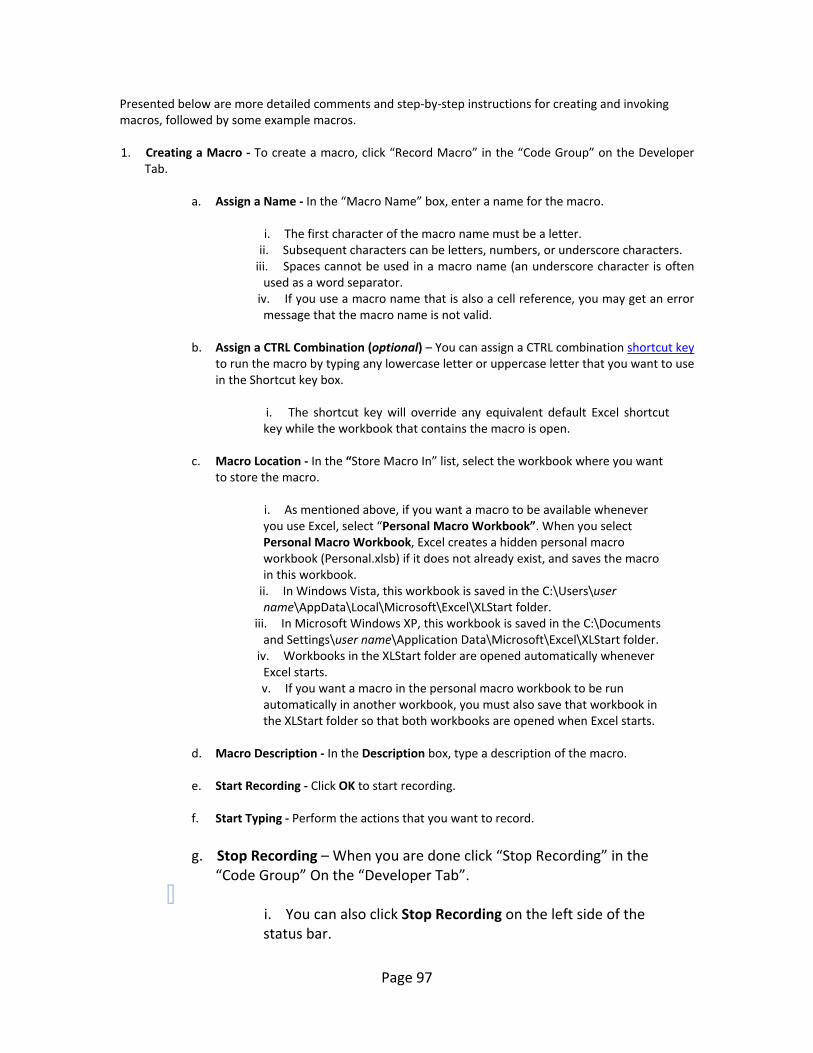
Page 97
Presented below are more detailed comments and step‐by‐step instructions for creating and invoking macros, followed by some example macros. 1. Creating a Macro ‐ To create a macro, click “Record Macro” in the “Code Group” on the Developer
Tab.
a. Assign a Name ‐ In the “Macro Name” box, enter a name for the macro.
i. The first character of the macro name must be a letter. ii. Subsequent characters can be letters, numbers, or underscore characters. iii. Spaces cannot be used in a macro name (an underscore character is often
used as a word separator. iv. If you use a macro name that is also a cell reference, you may get an error
message that the macro name is not valid.
b. Assign a CTRL Combination (optional) – You can assign a CTRL combination shortcut key to run the macro by typing any lowercase letter or uppercase letter that you want to use in the Shortcut key box.
i. The shortcut key will override any equivalent default Excel shortcut key while the workbook that contains the macro is open.
c. Macro Location ‐ In the “Store Macro In” list, select the workbook where you want
to store the macro.
i. As mentioned above, if you want a macro to be available whenever you use Excel, select “Personal Macro Workbook”. When you select Personal Macro Workbook, Excel creates a hidden personal macro workbook (Personal.xlsb) if it does not already exist, and saves the macro in this workbook.
ii. In Windows Vista, this workbook is saved in the C:\Users\user name\AppData\Local\Microsoft\Excel\XLStart folder.
iii. In Microsoft Windows XP, this workbook is saved in the C:\Documents and Settings\user name\Application Data\Microsoft\Excel\XLStart folder.
iv. Workbooks in the XLStart folder are opened automatically whenever Excel starts.
v. If you want a macro in the personal macro workbook to be run automatically in another workbook, you must also save that workbook in the XLStart folder so that both workbooks are opened when Excel starts.
d. Macro Description ‐ In the Description box, type a description of the macro.
e. Start Recording ‐ Click OK to start recording.
f. Start Typing ‐ Perform the actions that you want to record.
g. Stop Recording – When you are done click “Stop Recording” in the “Code Group” On the “Developer Tab”.
i. You can also click Stop Recording on the left side of the
status bar.
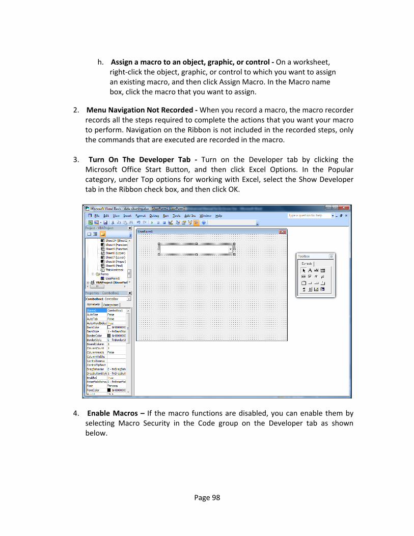
Page 98
h. Assign a macro to an object, graphic, or control ‐ On a worksheet,
right‐click the object, graphic, or control to which you want to assign an existing macro, and then click Assign Macro. In the Macro name box, click the macro that you want to assign.
2. Menu Navigation Not Recorded ‐ When you record a macro, the macro recorder
records all the steps required to complete the actions that you want your macro to perform. Navigation on the Ribbon is not included in the recorded steps, only the commands that are executed are recorded in the macro.
3. Turn On The Developer Tab ‐ Turn on the Developer tab by clicking the Microsoft Office Start Button, and then click Excel Options. In the Popular category, under Top options for working with Excel, select the Show Developer tab in the Ribbon check box, and then click OK.
4. Enable Macros – If the macro functions are disabled, you can enable them by selecting Macro Security in the Code group on the Developer tab as shown below.

Page 99
Under Macro Settings, click Enable all macros (not recommended, potentially dangerous code can run), and then click OK.
5. Example Macros
a. Page Setup Macro – Start recording a new macro called page setup.
Select all of the worksheets and then choose Page Setup and customize the header and footers to include page numbers, date and time stamps, file locations, tab names, etc. Assign the macro to an Icon on your toolbar or Quick Access Bar and insetting headers and footers will be a breeze for the rest of your life.
b. Print Macros – Do you have a template that you print frequently from? If so, insert several macro buttons to print each report, a group of reports, and even multiple reports and reporting will be snap in the future.
c. Delete Data Macro – Do you have a template that you use often that contains a lot of variables? If so, create a macro that visits each cell and erases that data, resetting the worksheet for use in a new set of criteria. Assign the macro to a macro button and you will never again have old assumptions mixed in with your newer template.

Page 100
Chapter 8
Solver
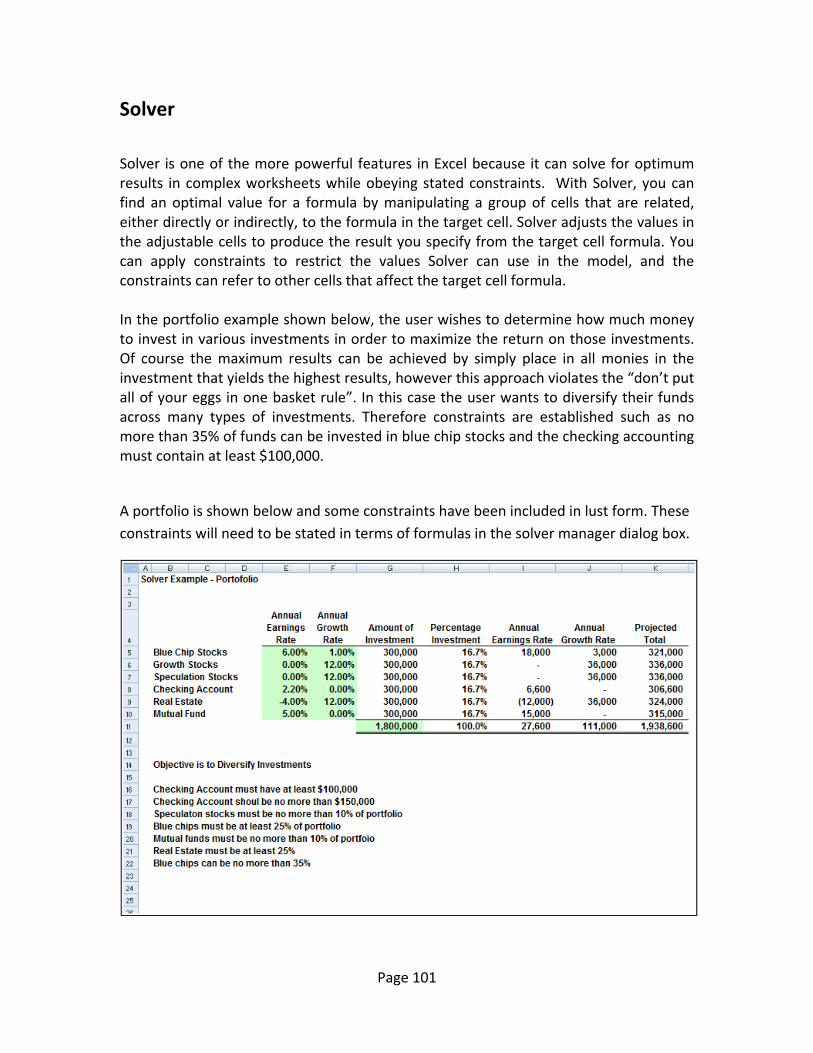
Page 101
Solver
Solver is one of the more powerful features in Excel because it can solve for optimum results in complex worksheets while obeying stated constraints. With Solver, you can find an optimal value for a formula by manipulating a group of cells that are related, either directly or indirectly, to the formula in the target cell. Solver adjusts the values in the adjustable cells to produce the result you specify from the target cell formula. You can apply constraints to restrict the values Solver can use in the model, and the constraints can refer to other cells that affect the target cell formula. In the portfolio example shown below, the user wishes to determine how much money to invest in various investments in order to maximize the return on those investments. Of course the maximum results can be achieved by simply place in all monies in the investment that yields the highest results, however this approach violates the “don’t put all of your eggs in one basket rule”. In this case the user wants to diversify their funds across many types of investments. Therefore constraints are established such as no more than 35% of funds can be invested in blue chip stocks and the checking accounting must contain at least $100,000.
A portfolio is shown below and some constraints have been included in lust form. These constraints will need to be stated in terms of formulas in the solver manager dialog box.
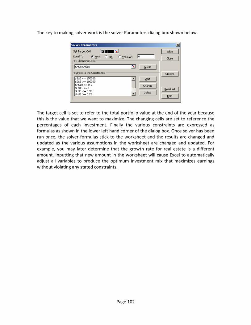
Page 102
The key to making solver work is the solver Parameters dialog box shown below.
The target cell is set to refer to the total portfolio value at the end of the year because this is the value that we want to maximize. The changing cells are set to reference the percentages of each investment. Finally the various constraints are expressed as formulas as shown in the lower left hand corner of the dialog box. Once solver has been run once, the solver formulas stick to the worksheet and the results are changed and updated as the various assumptions in the worksheet are changed and updated. For example, you may later determine that the growth rate for real estate is a different amount. Inputting that new amount in the worksheet will cause Excel to automatically adjust all variables to produce the optimum investment mix that maximizes earnings without violating any stated constraints.

Page 103
Chapter 9
EEXXAAMMPPLLEE Case Studies
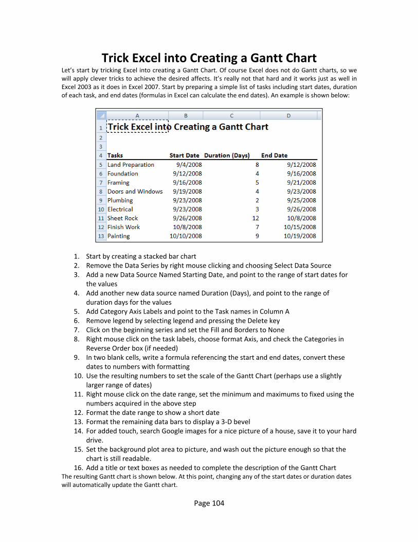
Page 104
Trick Excel into Creating a Gantt Chart Let’s start by tricking Excel into creating a Gantt Chart. Of course Excel does not do Gantt charts, so we will apply clever tricks to achieve the desired affects. It’s really not that hard and it works just as well in Excel 2003 as it does in Excel 2007. Start by preparing a simple list of tasks including start dates, duration of each task, and end dates (formulas in Excel can calculate the end dates). An example is shown below:
1. Start by creating a stacked bar chart 2. Remove the Data Series by right mouse clicking and choosing Select Data Source 3. Add a new Data Source Named Starting Date, and point to the range of start dates for
the values 4. Add another new data source named Duration (Days), and point to the range of
duration days for the values 5. Add Category Axis Labels and point to the Task names in Column A 6. Remove legend by selecting legend and pressing the Delete key 7. Click on the beginning series and set the Fill and Borders to None 8. Right mouse click on the task labels, choose format Axis, and check the Categories in
Reverse Order box (if needed) 9. In two blank cells, write a formula referencing the start and end dates, convert these
dates to numbers with formatting 10. Use the resulting numbers to set the scale of the Gantt Chart (perhaps use a slightly
larger range of dates) 11. Right mouse click on the date range, set the minimum and maximums to fixed using the
numbers acquired in the above step 12. Format the date range to show a short date 13. Format the remaining data bars to display a 3‐D bevel 14. For added touch, search Google images for a nice picture of a house, save it to your hard
drive. 15. Set the background plot area to picture, and wash out the picture enough so that the
chart is still readable. 16. Add a title or text boxes as needed to complete the description of the Gantt Chart
The resulting Gantt chart is shown below. At this point, changing any of the start dates or duration dates will automatically update the Gantt chart.
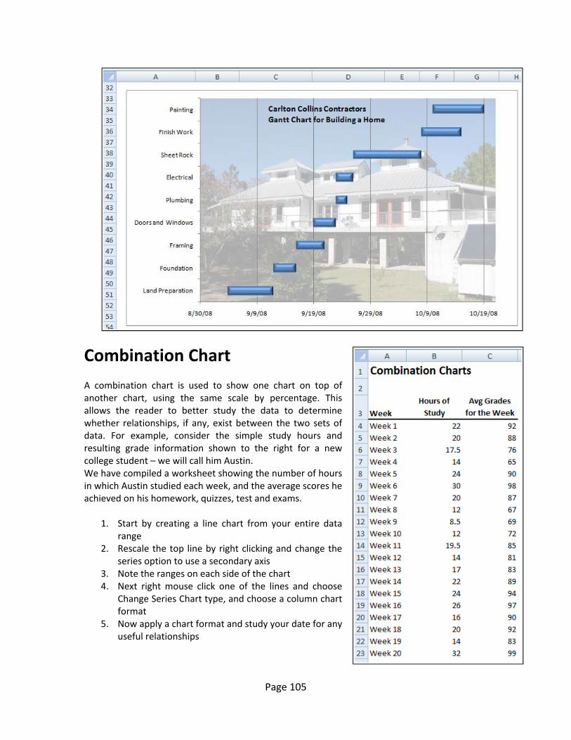
Page 105
Combination Chart A combination chart is used to show one chart on top of another chart, using the same scale by percentage. This allows the reader to better study the data to determine whether relationships, if any, exist between the two sets of data. For example, consider the simple study hours and resulting grade information shown to the right for a new college student – we will call him Austin. We have compiled a worksheet showing the number of hours in which Austin studied each week, and the average scores he achieved on his homework, quizzes, test and exams.
1. Start by creating a line chart from your entire data range
2. Rescale the top line by right clicking and change the series option to use a secondary axis
3. Note the ranges on each side of the chart 4. Next right mouse click one of the lines and choose
Change Series Chart type, and choose a column chart format
5. Now apply a chart format and study your date for any useful relationships
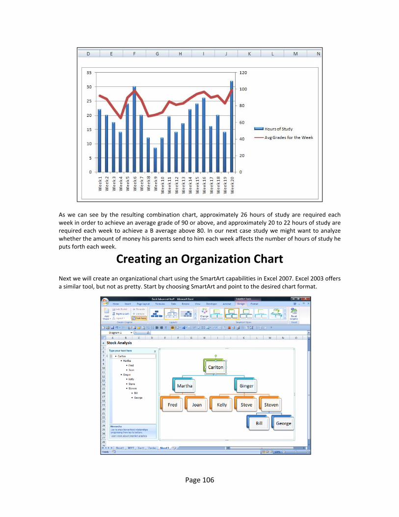
Page 106
As we can see by the resulting combination chart, approximately 26 hours of study are required each week in order to achieve an average grade of 90 or above, and approximately 20 to 22 hours of study are required each week to achieve a B average above 80. In our next case study we might want to analyze whether the amount of money his parents send to him each week affects the number of hours of study he puts forth each week.
Creating an Organization Chart Next we will create an organizational chart using the SmartArt capabilities in Excel 2007. Excel 2003 offers a similar tool, but not as pretty. Start by choosing SmartArt and point to the desired chart format.

Page 107
Portfolio Case Study The Situation ‐ Your individual client (Mr. Slade) has been very successful in his business dealings, and has accumulated $1 million in cash and investments. Previously Mr. Slade has invested these funds rather haphazardly, in a potpourri of investments without much strategy or thought. Presented below is a summary of his funds as they are currently invested:
Cash 275,000Speculative Stocks 400,000Mutual Funds 325,000
In speaking with Mr. Slade, with your help he determines that he would like to spread his investments around in a variety of investments in an effort to diversify his portfolio. Together, you come up with the following criteria for Mr. Slade’s investment strategy:
1. Mr. Slade wants to spread his investments around, including blue chip stocks, growth stocks, speculation stocks, cash, real estate and mutual funds.
2. Mr. Slade needs between $100,000 and $150,000 in liquid cash. 3. Mr. Slade wants to carry about 25% to 35% of the portfolio in blue chip stocks. 4. Mr. Slade would like to no more than 20% of the portfolio invested in speculative
stocks. 5. Mr. Slade wants no more than 20% of his investments in mutual funds.
The next step in this process is to estimate the expected return on investment (ROI) for each of investments. Some of these numbers are easy to come by and some are a little more difficult. For example, it is known that the checking account pays 2.2% interest, and of course there is no growth. Mr. Slade’s speculative stock investments have grown

Page 108
at an average of 12%, with no dividend payments while his mutual funds have grown 7% per year. A little research reveals that blue chip stocks grow on average 6.0% per year, and pay about 4% in dividends annually, and growth stocks grow at about 8% per year. The real estate market has shown steady growth of 12% per year, but there is an annual cost of about 3.5% for taxes, insurance and maintenance. Mr. Slade wants you to help him figure out which portfolio mix maximizes his earnings, while obeying his stated constraints. Thereafter, Mr. Slade wants you to set up a organized approach for tracking these investments in the future. The Big Picture ‐ Your Goals Are:
1. Install the Solver tool in Excel. 2. Use Solver to calculate the best mix of investments that also obeys Mr. Slade’s
stated investment goals and criteria.
3. Set up an Excel worksheet that organizes and tracks these investments.
4. Create web queries that will import stock prices and mutual fund information directly into Excel.
This Case Study Covers the following Excel Features and Concepts:
1. Add‐ins 2. Solver Overview 3. Solver Worksheet 4. Solver Constraints 5. Solver Targets 6. Solver Reporting 7. Portfolio Design 8. Web Queries
9. Web Query Parameters 10. Editing Web Queries 11. Refreshing Web Queries 12. Subtotaling 13. Outlining 14. Tables 15. PivotTables 16. Format Gallery
Steps:
1. To use the Solver Add‐in, you need to load it first. To do this, Click the Microsoft Office Button, and then click Excel Options. Click Add‐Ins, and then in the Manage box, select Excel Add‐ins. Click Go. In the Add‐Ins available box, select the Solver Add‐in check box, and then click OK. After you load the Solver Add‐in, the Solver command is available in the Analysis group on the Data tab.
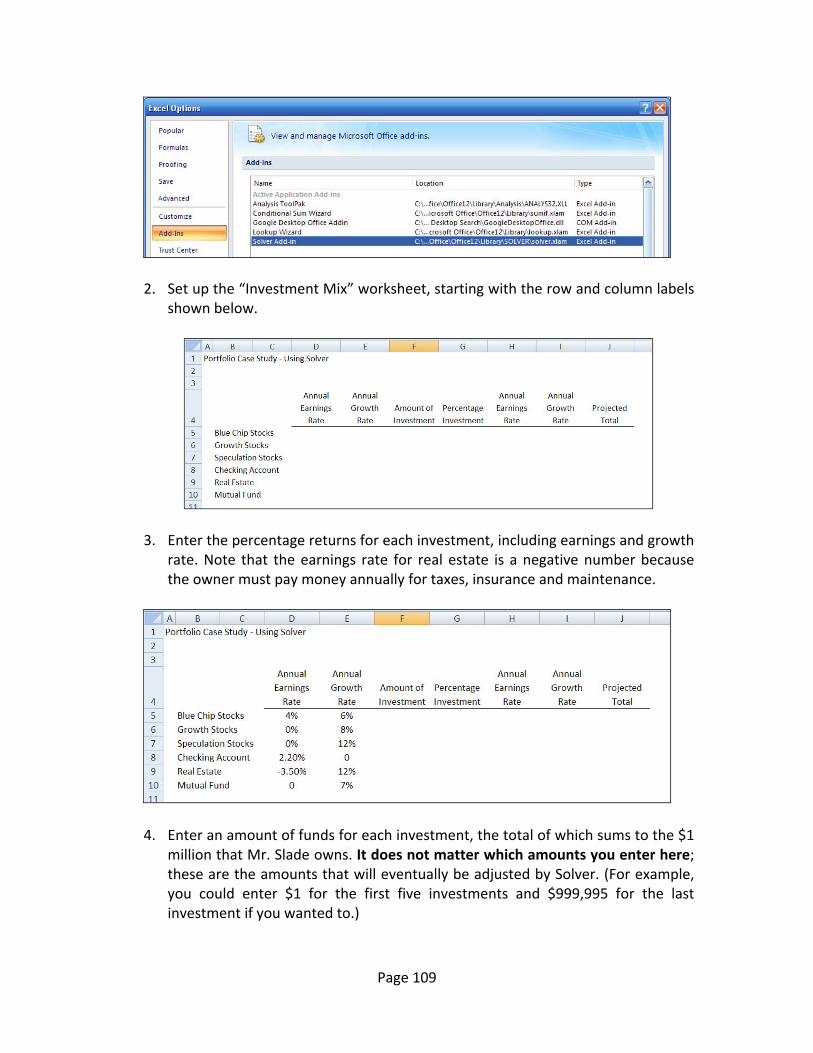
Page 109
2. Set up the “Investment Mix” worksheet, starting with the row and column labels shown below.
3. Enter the percentage returns for each investment, including earnings and growth rate. Note that the earnings rate for real estate is a negative number because the owner must pay money annually for taxes, insurance and maintenance.
4. Enter an amount of funds for each investment, the total of which sums to the $1 million that Mr. Slade owns. It does not matter which amounts you enter here; these are the amounts that will eventually be adjusted by Solver. (For example, you could enter $1 for the first five investments and $999,995 for the last investment if you wanted to.)
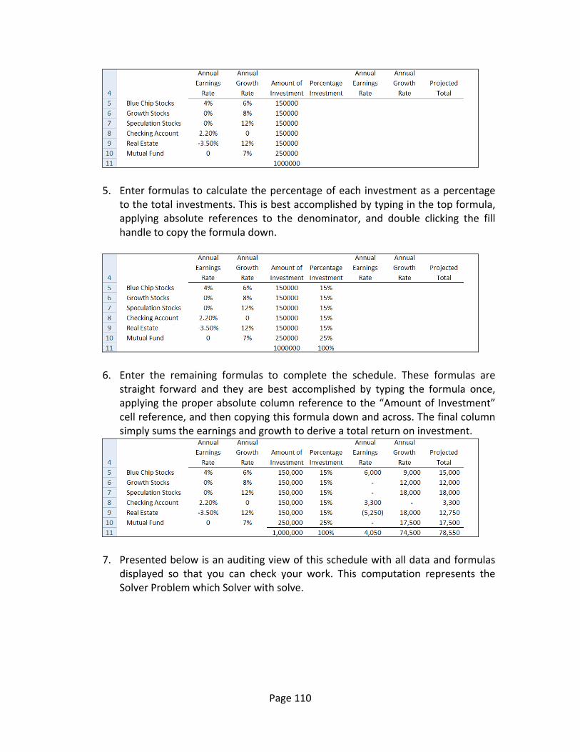
Page 110
5. Enter formulas to calculate the percentage of each investment as a percentage to the total investments. This is best accomplished by typing in the top formula, applying absolute references to the denominator, and double clicking the fill handle to copy the formula down.
6. Enter the remaining formulas to complete the schedule. These formulas are straight forward and they are best accomplished by typing the formula once, applying the proper absolute column reference to the “Amount of Investment” cell reference, and then copying this formula down and across. The final column simply sums the earnings and growth to derive a total return on investment.
7. Presented below is an auditing view of this schedule with all data and formulas displayed so that you can check your work. This computation represents the Solver Problem which Solver with solve.
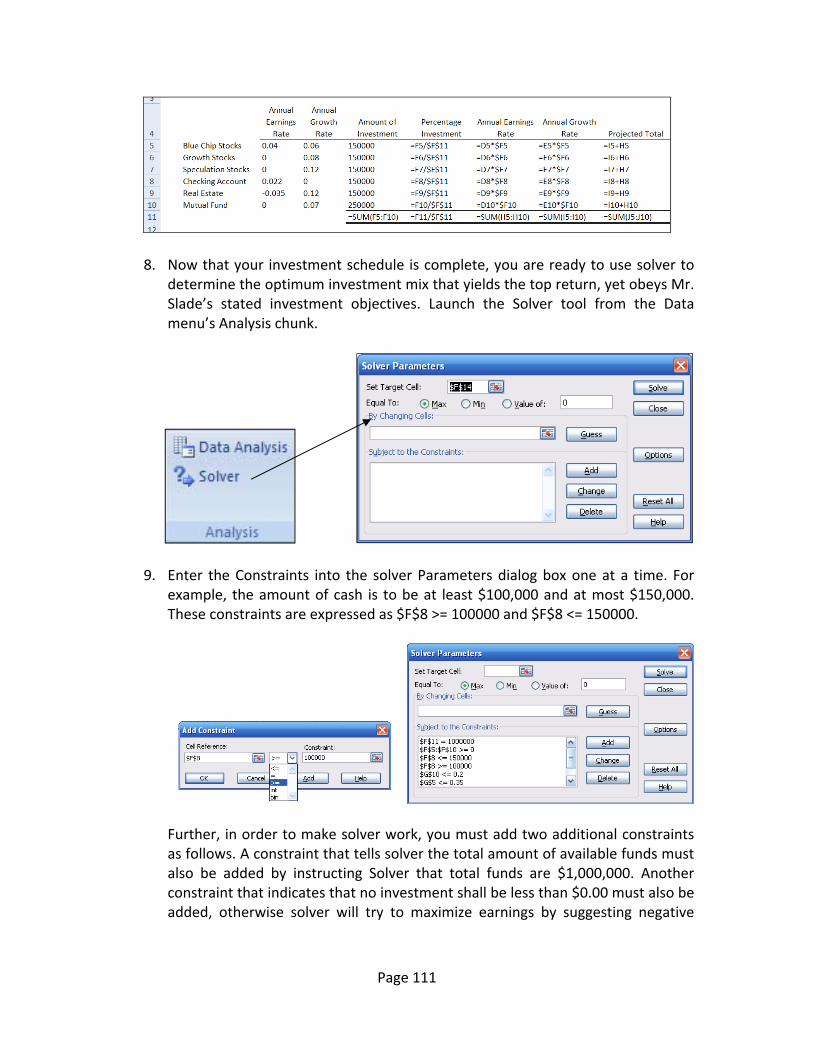
Page 111
8. Now that your investment schedule is complete, you are ready to use solver to determine the optimum investment mix that yields the top return, yet obeys Mr. Slade’s stated investment objectives. Launch the Solver tool from the Data menu’s Analysis chunk.
9. Enter the Constraints into the solver Parameters dialog box one at a time. For example, the amount of cash is to be at least $100,000 and at most $150,000. These constraints are expressed as $F$8 >= 100000 and $F$8 <= 150000.
Further, in order to make solver work, you must add two additional constraints as follows. A constraint that tells solver the total amount of available funds must also be added by instructing Solver that total funds are $1,000,000. Another constraint that indicates that no investment shall be less than $0.00 must also be added, otherwise solver will try to maximize earnings by suggesting negative
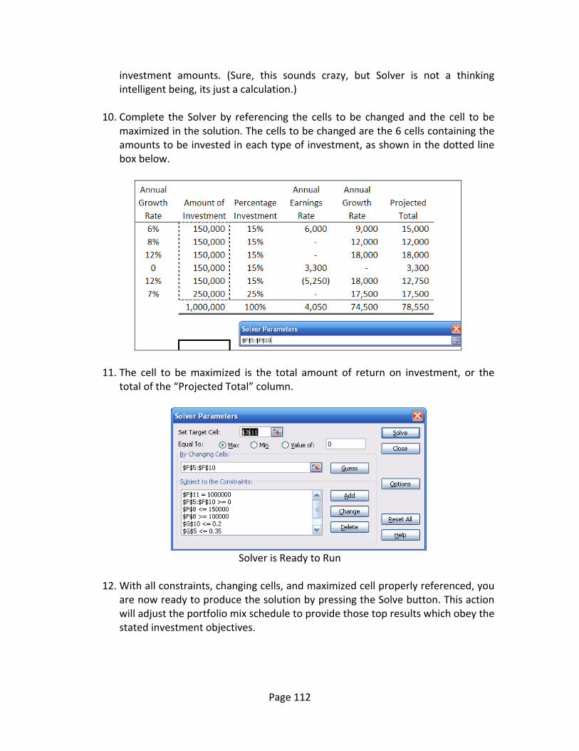
Page 112
investment amounts. (Sure, this sounds crazy, but Solver is not a thinking intelligent being, its just a calculation.)
10. Complete the Solver by referencing the cells to be changed and the cell to be
maximized in the solution. The cells to be changed are the 6 cells containing the amounts to be invested in each type of investment, as shown in the dotted line box below.
11. The cell to be maximized is the total amount of return on investment, or the
total of the “Projected Total” column.
Solver is Ready to Run
12. With all constraints, changing cells, and maximized cell properly referenced, you
are now ready to produce the solution by pressing the Solve button. This action will adjust the portfolio mix schedule to provide those top results which obey the stated investment objectives.

Page 113
As you can see by the serene above, solver has adjusted the portfolio investment mix to show that total earnings of $90,950 can be achieved by maximizing the investments in blue chip stocks, avoiding growth stocks, placing the minimum amount of $100,000 in checking, etc. After producing this report, Mr. Slade may decide that additional constraints are needed, and if so, the numbers can be massaged accordingly.
13. Solver now offers a variety of options for reporting the results. The report can be
saved as a scenario. Thereafter, Solver will produce various reports to help you understand the results. The first of these reports is the Answers Report shown to the right.
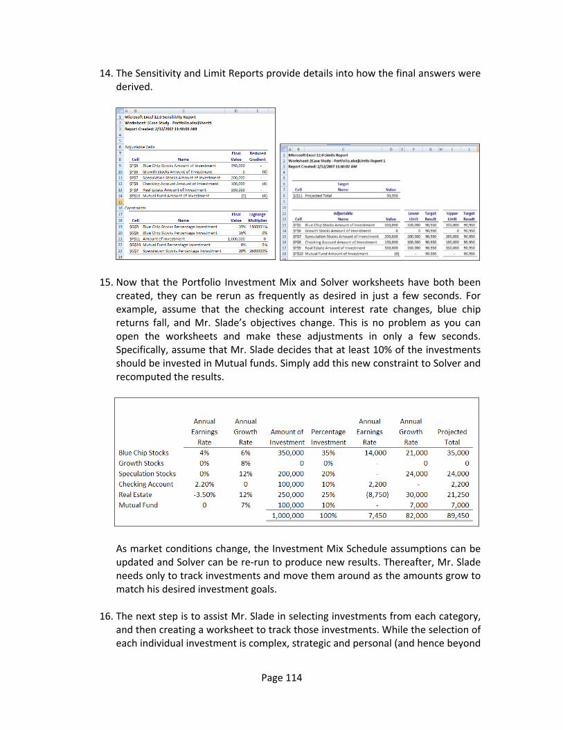
Page 114
14. The Sensitivity and Limit Reports provide details into how the final answers were derived.
15. Now that the Portfolio Investment Mix and Solver worksheets have both been created, they can be rerun as frequently as desired in just a few seconds. For example, assume that the checking account interest rate changes, blue chip returns fall, and Mr. Slade’s objectives change. This is no problem as you can open the worksheets and make these adjustments in only a few seconds. Specifically, assume that Mr. Slade decides that at least 10% of the investments should be invested in Mutual funds. Simply add this new constraint to Solver and recomputed the results.
As market conditions change, the Investment Mix Schedule assumptions can be updated and Solver can be re‐run to produce new results. Thereafter, Mr. Slade needs only to track investments and move them around as the amounts grow to match his desired investment goals.
16. The next step is to assist Mr. Slade in selecting investments from each category,
and then creating a worksheet to track those investments. While the selection of each individual investment is complex, strategic and personal (and hence beyond
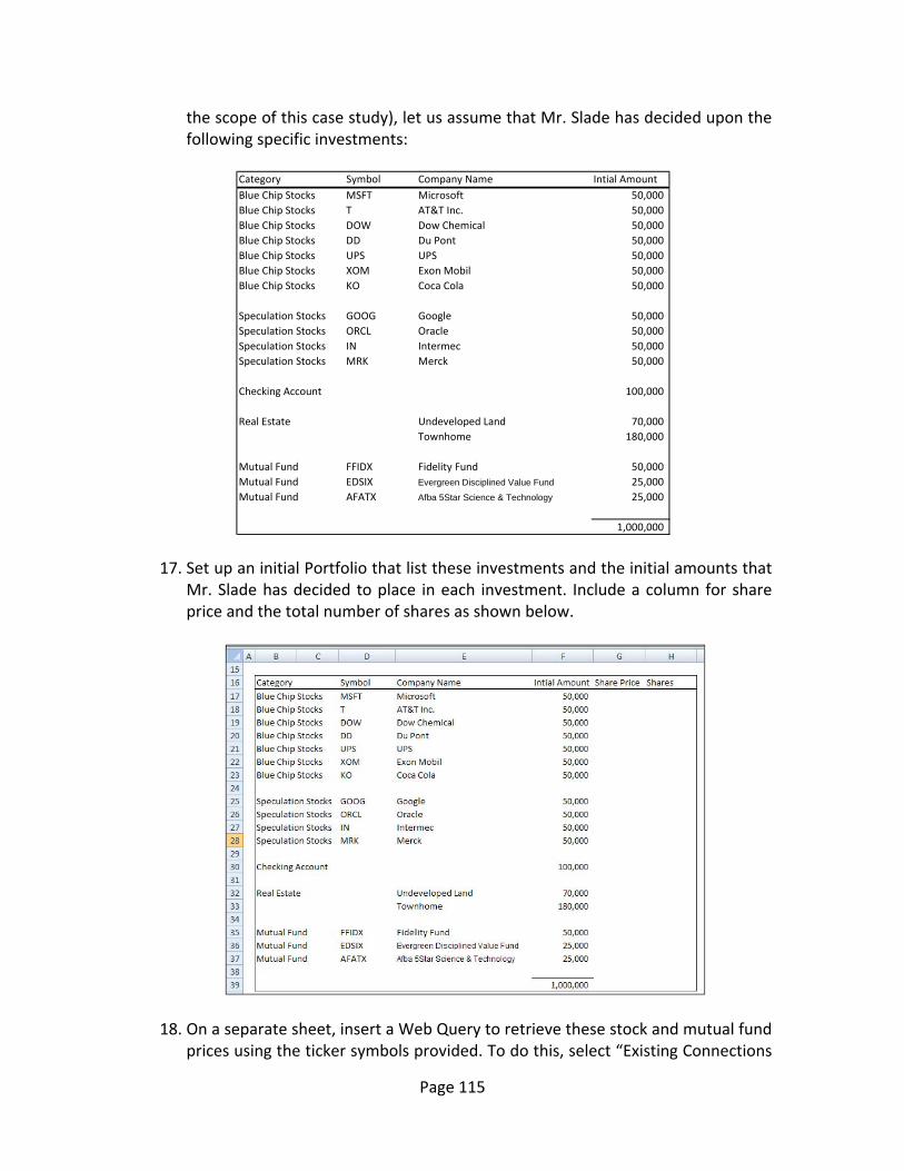
Page 115
the scope of this case study), let us assume that Mr. Slade has decided upon the following specific investments:
17. Set up an initial Portfolio that list these investments and the initial amounts that Mr. Slade has decided to place in each investment. Include a column for share price and the total number of shares as shown below.
18. On a separate sheet, insert a Web Query to retrieve these stock and mutual fund prices using the ticker symbols provided. To do this, select “Existing Connections
Category Symbol Company Name Intial AmountBlue Chip Stocks MSFT Microsoft 50,000 Blue Chip Stocks T AT&T Inc. 50,000 Blue Chip Stocks DOW Dow Chemical 50,000 Blue Chip Stocks DD Du Pont 50,000 Blue Chip Stocks UPS UPS 50,000 Blue Chip Stocks XOM Exon Mobil 50,000 Blue Chip Stocks KO Coca Cola 50,000
Speculation Stocks GOOG Google 50,000 Speculation Stocks ORCL Oracle 50,000 Speculation Stocks IN Intermec 50,000 Speculation Stocks MRK Merck 50,000
Checking Account 100,000
Real Estate Undeveloped Land 70,000 Townhome 180,000
Mutual Fund FFIDX Fidelity Fund 50,000 Mutual Fund EDSIX Evergreen Disciplined Value Fund 25,000 Mutual Fund AFATX Afba 5Star Science & Technology 25,000
1,000,000
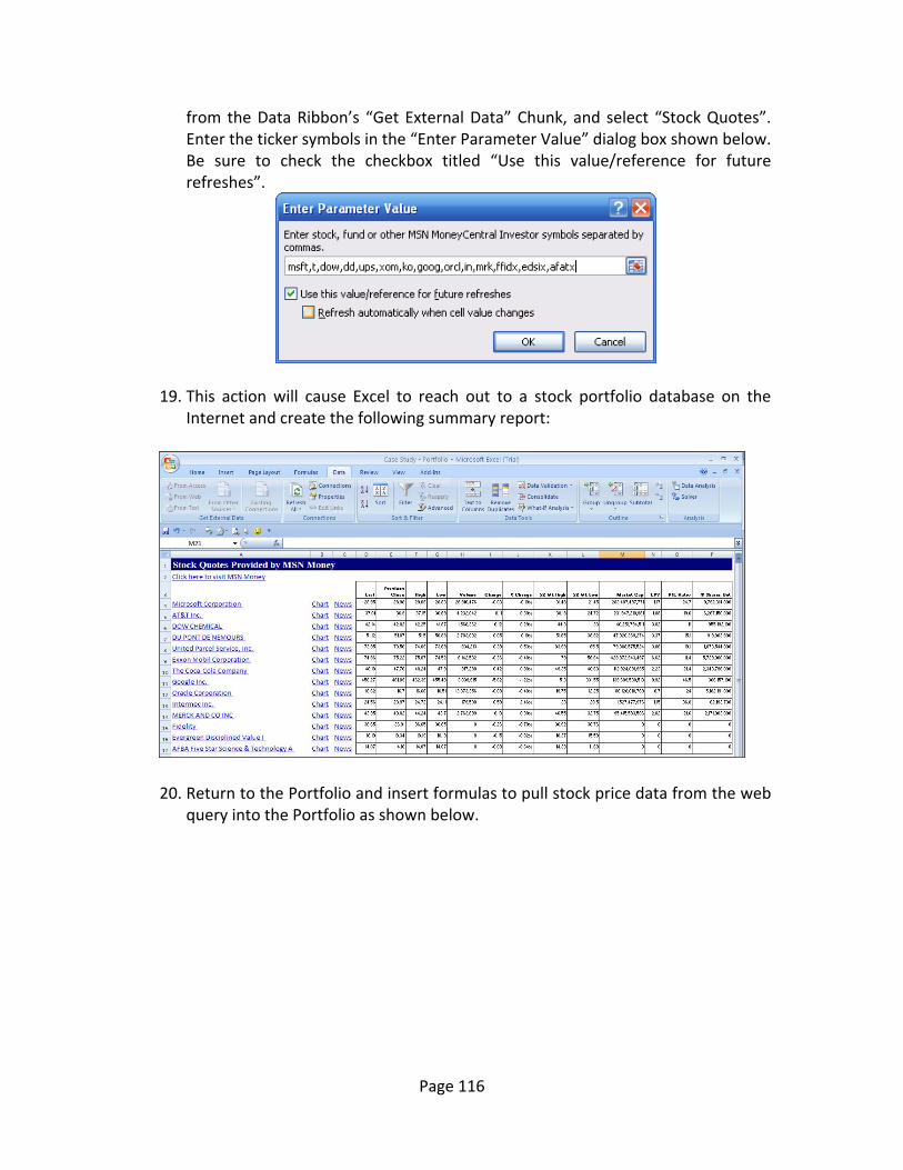
Page 116
from the Data Ribbon’s “Get External Data” Chunk, and select “Stock Quotes”. Enter the ticker symbols in the “Enter Parameter Value” dialog box shown below. Be sure to check the checkbox titled “Use this value/reference for future refreshes”.
19. This action will cause Excel to reach out to a stock portfolio database on the Internet and create the following summary report:
20. Return to the Portfolio and insert formulas to pull stock price data from the web
query into the Portfolio as shown below.

Page 117
21. Add formulas in the shares column by dividing the amount of each investment by
the share price in order to determine the appropriate number of shares of each investment Mr. Slade should purchase to meet his investment goals. Be sure to use the round function and round to the nearest tenth.
22. Once Mr. Slade has made all of the necessary investments, recreate the portfolio
on a new sheet, and make the necessary adjustments to reflect the actual results of these transactions. Due to the requirements of purchasing bocks of shares, Mr. Slade will not be able to purchase the exact number of shares indicated above at the exact same price indicated above. Therefore there will be slight discrepancies. Once those transactions are completed, Mr. Slade will need a worksheet that documents the beginning point in which Mr. Slade begins to track his investments. For example, the resulting Portfolio might look like this:
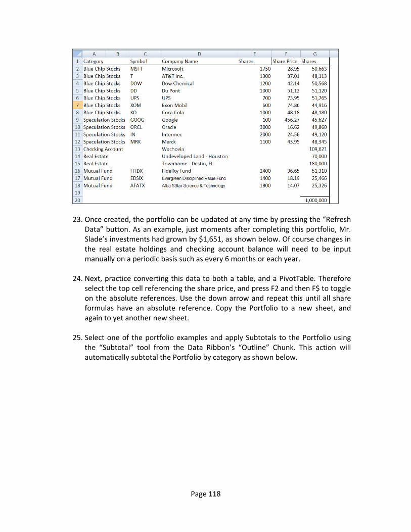
Page 118
23. Once created, the portfolio can be updated at any time by pressing the “Refresh Data” button. As an example, just moments after completing this portfolio, Mr. Slade’s investments had grown by $1,651, as shown below. Of course changes in the real estate holdings and checking account balance will need to be input manually on a periodic basis such as every 6 months or each year.
24. Next, practice converting this data to both a table, and a PivotTable. Therefore
select the top cell referencing the share price, and press F2 and then F$ to toggle on the absolute references. Use the down arrow and repeat this until all share formulas have an absolute reference. Copy the Portfolio to a new sheet, and again to yet another new sheet.
25. Select one of the portfolio examples and apply Subtotals to the Portfolio using
the “Subtotal” tool from the Data Ribbon’s “Outline” Chunk. This action will automatically subtotal the Portfolio by category as shown below.
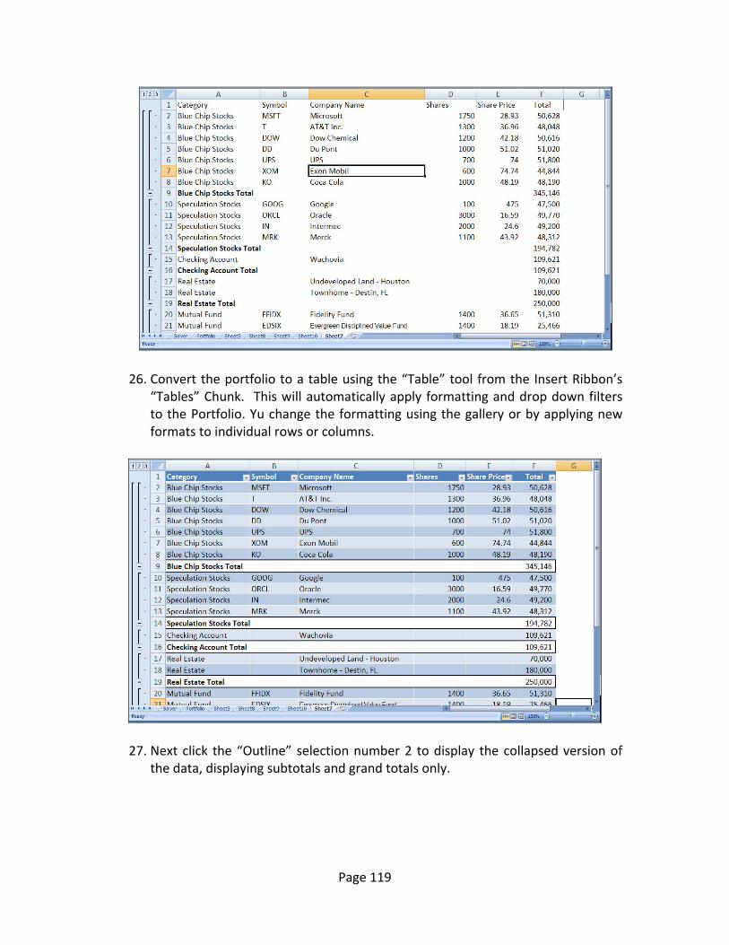
Page 119
26. Convert the portfolio to a table using the “Table” tool from the Insert Ribbon’s
“Tables” Chunk. This will automatically apply formatting and drop down filters to the Portfolio. Yu change the formatting using the gallery or by applying new formats to individual rows or columns.
27. Next click the “Outline” selection number 2 to display the collapsed version of the data, displaying subtotals and grand totals only.
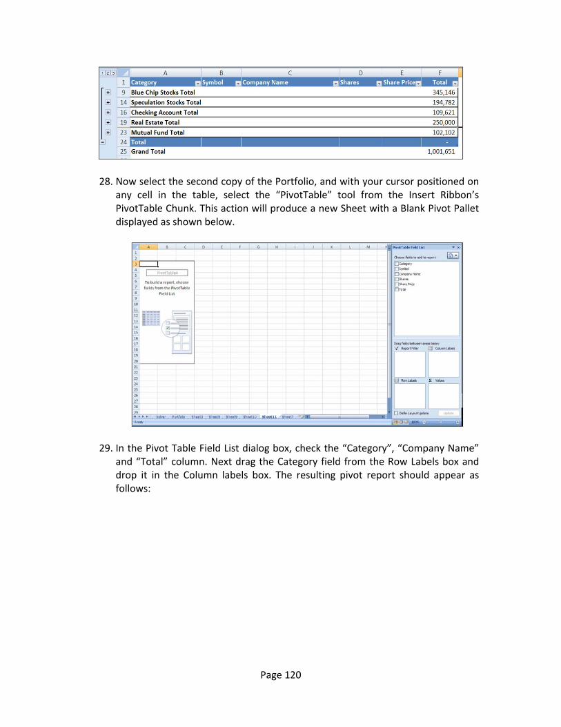
Page 120
28. Now select the second copy of the Portfolio, and with your cursor positioned on any cell in the table, select the “PivotTable” tool from the Insert Ribbon’s PivotTable Chunk. This action will produce a new Sheet with a Blank Pivot Pallet displayed as shown below.
29. In the Pivot Table Field List dialog box, check the “Category”, “Company Name” and “Total” column. Next drag the Category field from the Row Labels box and drop it in the Column labels box. The resulting pivot report should appear as follows:
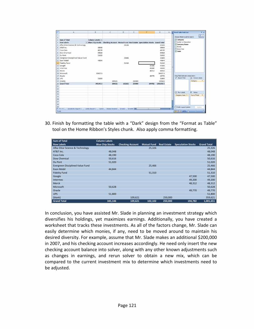
Page 121
30. Finish by formatting the table with a “Dark” design from the “Format as Table” tool on the Home Ribbon’s Styles chunk. Also apply comma formatting.
In conclusion, you have assisted Mr. Slade in planning an investment strategy which diversifies his holdings, yet maximizes earnings. Additionally, you have created a worksheet that tracks these investments. As all of the factors change, Mr. Slade can easily determine which monies, if any, need to be moved around to maintain his desired diversity. For example, assume that Mr. Slade makes an additional $200,000 in 2007, and his checking account increases accordingly. He need only insert the new checking account balance into solver, along with any other known adjustments such as changes in earnings, and rerun solver to obtain a new mix, which can be compared to the current investment mix to determine which investments need to be adjusted.
Sum of Total Column LabelsRow Labels Blue Chip Stocks Checking Account Mutual Fund Real Estate Speculation Stocks Grand TotalAfba 5Star Science & Technology 25,326 25,326 AT&T Inc. 48,048 48,048 Coca Cola 48,190 48,190 Dow Chemical 50,616 50,616 Du Pont 51,020 51,020 Evergreen Disciplined Value Fund 25,466 25,466 Exon Mobil 44,844 44,844 Fidelity Fund 51,310 51,310 Google 47,500 47,500 Intermec 49,200 49,200 Merck 48,312 48,312 Microsoft 50,628 50,628 Oracle 49,770 49,770 UPS 51,800 51,800 (blank) 109,621 250,000 359,621 Grand Total 345,146 109,621 102,102 250,000 194,782 1,001,651
Page 122
Chapter 10
Excel Advanced Digging Deeper into
Excel’s Fundamentals
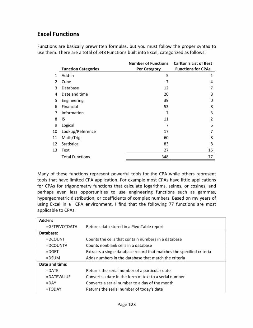
Page 123
Excel Functions
Functions are basically prewritten formulas, but you must follow the proper syntax to use them. There are a total of 348 Functions built into Excel, categorized as follows:
Function Categories Number of Functions
Per Category Carlton's List of Best Functions for CPAs
1 Add‐in 5 12 Cube 7 43 Database 12 74 Date and time 20 85 Engineering 39 06 Financial 53 87 Information 7 38 IS 11 29 Logical 7 6
10 Lookup/Reference 17 711 Math/Trig 60 812 Statistical 83 813 Text 27 15
Total Functions 348 77
Many of these functions represent powerful tools for the CPA while others represent tools that have limited CPA application. For example most CPAs have little applications for CPAs for trigonometry functions that calculate logarithms, seines, or cosines, and perhaps even less opportunities to use engineering functions such as gammas, hypergeometric distribution, or coefficients of complex numbers. Based on my years of using Excel in a CPA environment, I find that the following 77 functions are most applicable to CPAs:
Add‐in: =GETPIVOTDATA Returns data stored in a PivotTable report Database: =DCOUNT Counts the cells that contain numbers in a database =DCOUNTA Counts nonblank cells in a database =DGET Extracts a single database record that matches the specified criteria =DSUM Adds numbers in the database that match the criteria Date and time: =DATE Returns the serial number of a particular date =DATEVALUE Converts a date in the form of text to a serial number =DAY Converts a serial number to a day of the month =TODAY Returns the serial number of today's date
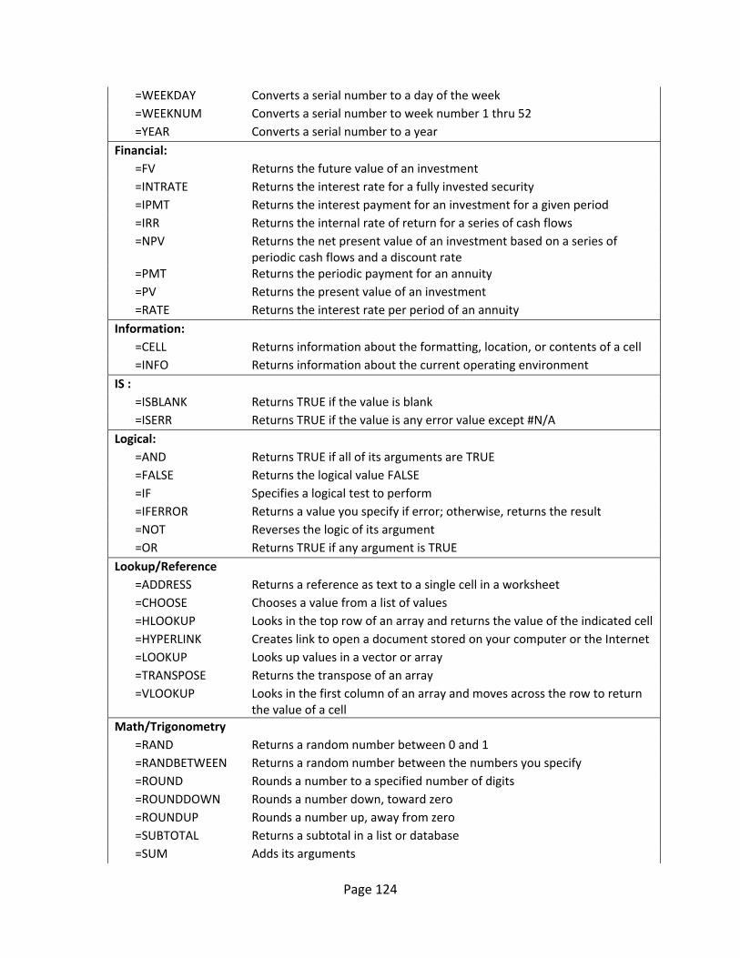
Page 124
=WEEKDAY Converts a serial number to a day of the week =WEEKNUM Converts a serial number to week number 1 thru 52 =YEAR Converts a serial number to a year Financial: =FV Returns the future value of an investment =INTRATE Returns the interest rate for a fully invested security =IPMT Returns the interest payment for an investment for a given period =IRR Returns the internal rate of return for a series of cash flows =NPV Returns the net present value of an investment based on a series of
periodic cash flows and a discount rate =PMT Returns the periodic payment for an annuity =PV Returns the present value of an investment =RATE Returns the interest rate per period of an annuity Information: =CELL Returns information about the formatting, location, or contents of a cell =INFO Returns information about the current operating environment IS : =ISBLANK Returns TRUE if the value is blank =ISERR Returns TRUE if the value is any error value except #N/A Logical: =AND Returns TRUE if all of its arguments are TRUE =FALSE Returns the logical value FALSE =IF Specifies a logical test to perform =IFERROR Returns a value you specify if error; otherwise, returns the result =NOT Reverses the logic of its argument =OR Returns TRUE if any argument is TRUE Lookup/Reference =ADDRESS Returns a reference as text to a single cell in a worksheet =CHOOSE Chooses a value from a list of values =HLOOKUP Looks in the top row of an array and returns the value of the indicated cell =HYPERLINK Creates link to open a document stored on your computer or the Internet =LOOKUP Looks up values in a vector or array =TRANSPOSE Returns the transpose of an array =VLOOKUP Looks in the first column of an array and moves across the row to return
the value of a cell Math/Trigonometry =RAND Returns a random number between 0 and 1 =RANDBETWEEN Returns a random number between the numbers you specify =ROUND Rounds a number to a specified number of digits =ROUNDDOWN Rounds a number down, toward zero =ROUNDUP Rounds a number up, away from zero =SUBTOTAL Returns a subtotal in a list or database =SUM Adds its arguments
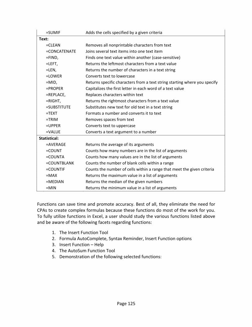
Page 125
=SUMIF Adds the cells specified by a given criteria Text: =CLEAN Removes all nonprintable characters from text =CONCATENATE Joins several text items into one text item =FIND, Finds one text value within another (case‐sensitive) =LEFT, Returns the leftmost characters from a text value =LEN, Returns the number of characters in a text string =LOWER Converts text to lowercase =MID, Returns specific characters from a text string starting where you specify =PROPER Capitalizes the first letter in each word of a text value =REPLACE, Replaces characters within text =RIGHT, Returns the rightmost characters from a text value =SUBSTITUTE Substitutes new text for old text in a text string =TEXT Formats a number and converts it to text =TRIM Removes spaces from text =UPPER Converts text to uppercase =VALUE Converts a text argument to a number Statistical: =AVERAGE Returns the average of its arguments =COUNT Counts how many numbers are in the list of arguments =COUNTA Counts how many values are in the list of arguments =COUNTBLANK Counts the number of blank cells within a range =COUNTIF Counts the number of cells within a range that meet the given criteria =MAX Returns the maximum value in a list of arguments =MEDIAN Returns the median of the given numbers =MIN Returns the minimum value in a list of arguments
Functions can save time and promote accuracy. Best of all, they eliminate the need for CPAs to create complex formulas because these functions do most of the work for you. To fully utilize functions in Excel, a user should study the various functions listed above and be aware of the following facets regarding functions:
1. The Insert Function Tool 2. Formula AutoComplete, Syntax Reminder, Insert Function options 3. Insert Function – Help 4. The AutoSum Function Tool 5. Demonstration of the following selected functions:
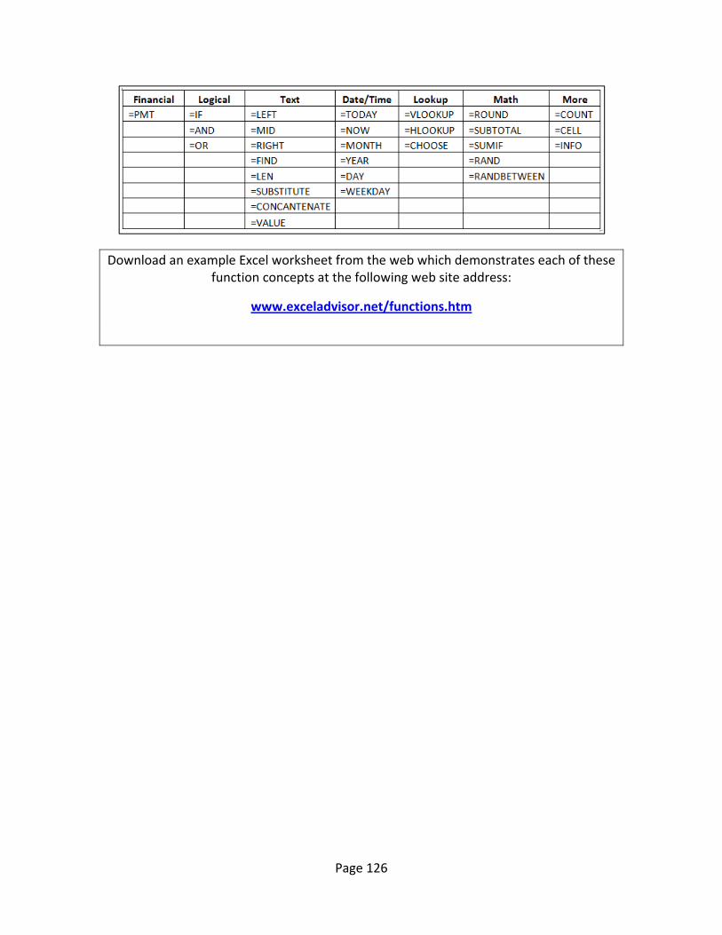
Page 126
Download an example Excel worksheet from the web which demonstrates each of these function concepts at the following web site address:
www.exceladvisor.net/functions.htm
Page 127
Formatting: Formulas and Functions represent the power Excel has to offer, but your final product must be neat, readable, and well‐organized. Excel’s built‐in formatting tools are designed to help you produce financial reports and data that are of presentation quality. The key formatting concepts that CPA’s should be aware of are as follows:
1. Number Formats – Controlling commas, decimals, currency symbols, and negatives.
2. Date Formats – Controlling days, months, years, seconds, hours and minute. 3. Alignment ‐ Left, Middle, Right, Top, Middle, & Bottom. 4. Alignment – Text Wrapping. 5. Alignment – Text Orientation. 6. Alignment – Text Shrink to Fit. 7. Alignment – Text Direction. 8. Fonts ‐ Font Size, Bold, Italics, Color. 9. Fonts – Strikethroughs, Superscripts & Subscripts. 10. Fonts – In‐Cell Formatting Character‐by‐Character. 11. Fonts – Underlines & Double Underlines. 12. Cells – Borders, Colors & Line Styles. 13. Cells – Fill Colors & Fill Effects. 14. Cells – Merging Cells. 15. Cells ‐ Fill Color, Pattern, Effect. 16. Conditional Formatting – Highlighting with Colors. 17. Conditional Formatting – Top & Bottom Formatting. 18. Conditional Formatting – Data Bars. 19. Conditional Formatting – Traffic Lights. 20. Column Width and Row Height – Changing one row or column. 21. Column Width and Row Height – Changing multiple rows or columns. 22. Column Width and Row Height – Auto adjusting row height and columns widths. 23. Styles – Using Excel’s Default Styles. 24. Styles – Creating Custom Styles. 25. Tables – Table Formatting.
Download an example Excel worksheet from the web which demonstrates each of these formatting concepts at the following web site address:
www.exceladvisor.net/formetting.htm
Page 128
Microsoft Excel XML Chapter 11
Page 129
Overview of XML in Excel Hide All Microsoft Office Excel makes it easy to import Extensible Markup Language (XML) (Extensible Markup Language (XML): A condensed form of Standard Generalized Markup Language (SGML) that enables developers to create customized tags that offer flexibility in organizing and presenting information.) data that is created from other databases and applications, to map XML elements from an XML schema (XML Schema: A formal specification, written in XML, that defines the structure of an XML document, including element names and rich data types, which elements can appear in combination, and which attributes are available for each element.) to worksheet cells, and to export revised XML data for interaction with other databases and applications. Think of these XML features as turning Office Excel into an XML data file generator with a familiar user interface.
1. Why use XML in Excel?
a. XML data and schema files b. Key XML and Excel scenarios
2. The basic process of using XML data in Excel a. Working with XML maps b. Using the XML Source task pane c. Element types and their icons d. Working with single‐mapped cells e. Working with repeating cells in XML tables f. XML map security considerations g. Importing XML data h. Working with an inferred schema i. Exporting XML data
3. Using the Excel macro‐enabled Office XML Format file
Why use XML in Excel? XML is a technology that is designed for managing and sharing structured data in a human‐readable text file. XML follows industry‐standard guidelines and can be processed by a variety of databases and applications. Using XML, application designers can create their own customized tags, data structures, and schemas. In short, XML greatly eases the definition, transmission, validation, and interpretation of data between databases, applications, and organizations. XML data and schema files Excel works primarily with two types of XML files:
XML data files (.xml), which contain the custom tags and structured data. Schema files (.xsd), which contain schema tags that enforce rules, such as data type and validation. Note The XML standard also defines Extensible Stylesheet Language Transformation (XSLT) (XSL Transformation (XSLT): A file that is used to transform XML documents into other types of documents, such as HTML or XML. It is designed for use as part of XSL.) (.xslt) files, which are used to apply styles and transform XML data into different presentation formats. You can apply these transforms before you import XML files into Excel and after you export XML files from Excel. If XSLT files are linked to XML data files that you import into Excel, you do have the
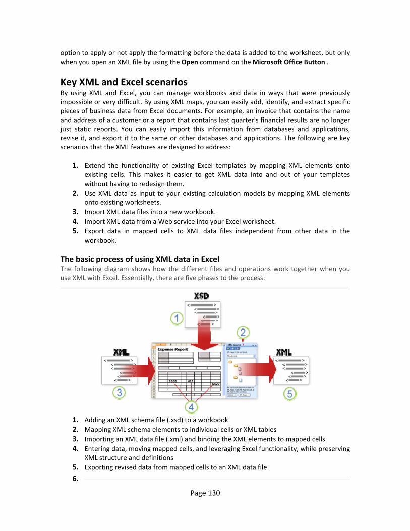
Page 130
option to apply or not apply the formatting before the data is added to the worksheet, but only when you open an XML file by using the Open command on the Microsoft Office Button .
Key XML and Excel scenarios By using XML and Excel, you can manage workbooks and data in ways that were previously impossible or very difficult. By using XML maps, you can easily add, identify, and extract specific pieces of business data from Excel documents. For example, an invoice that contains the name and address of a customer or a report that contains last quarter's financial results are no longer just static reports. You can easily import this information from databases and applications, revise it, and export it to the same or other databases and applications. The following are key scenarios that the XML features are designed to address:
1. Extend the functionality of existing Excel templates by mapping XML elements onto existing cells. This makes it easier to get XML data into and out of your templates without having to redesign them.
2. Use XML data as input to your existing calculation models by mapping XML elements onto existing worksheets.
3. Import XML data files into a new workbook. 4. Import XML data from a Web service into your Excel worksheet. 5. Export data in mapped cells to XML data files independent from other data in the
workbook. The basic process of using XML data in Excel The following diagram shows how the different files and operations work together when you use XML with Excel. Essentially, there are five phases to the process:
1. Adding an XML schema file (.xsd) to a workbook 2. Mapping XML schema elements to individual cells or XML tables 3. Importing an XML data file (.xml) and binding the XML elements to mapped cells 4. Entering data, moving mapped cells, and leveraging Excel functionality, while preserving
XML structure and definitions 5. Exporting revised data from mapped cells to an XML data file
6.
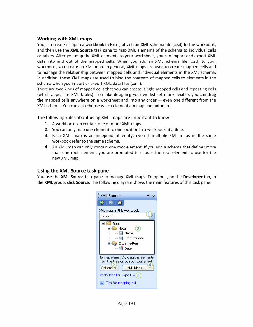
Page 131
Working with XML maps You can create or open a workbook in Excel, attach an XML schema file (.xsd) to the workbook, and then use the XML Source task pane to map XML elements of the schema to individual cells or tables. After you map the XML elements to your worksheet, you can import and export XML data into and out of the mapped cells. When you add an XML schema file (.xsd) to your workbook, you create an XML map. In general, XML maps are used to create mapped cells and to manage the relationship between mapped cells and individual elements in the XML schema. In addition, these XML maps are used to bind the contents of mapped cells to elements in the schema when you import or export XML data files (.xml). There are two kinds of mapped cells that you can create: single‐mapped cells and repeating cells (which appear as XML tables). To make designing your worksheet more flexible, you can drag the mapped cells anywhere on a worksheet and into any order — even one different from the XML schema. You can also choose which elements to map and not map. The following rules about using XML maps are important to know:
1. A workbook can contain one or more XML maps. 2. You can only map one element to one location in a workbook at a time. 3. Each XML map is an independent entity, even if multiple XML maps in the same
workbook refer to the same schema. 4. An XML map can only contain one root element. If you add a schema that defines more
than one root element, you are prompted to choose the root element to use for the new XML map.
Using the XML Source task pane You use the XML Source task pane to manage XML maps. To open it, on the Developer tab, in the XML group, click Source. The following diagram shows the main features of this task pane.
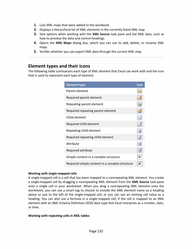
Page 132
1. Lists XML maps that were added to the workbook 2. Displays a hierarchical list of XML elements in the currently listed XML map 3. Sets options when working with the XML Source task pane and the XML data, such as
how to preview the data and control headings 4. Opens the XML Maps dialog box, which you can use to add, delete, or rename XML
maps 5. Verifies whether you can export XML data through the current XML map
Element types and their icons The following table summarizes each type of XML element that Excel can work with and the icon that is used to represent each type of element.
Element type Icon
Parent element
Required parent element
Repeating parent element
Required repeating parent element
Child element
Required child element
Repeating child element
Required repeating child element
Attribute
Required attribute
Simple content in a complex structure
Required simple content in a complex structure Working with single‐mapped cells A single‐mapped cell is a cell that has been mapped to a nonrepeating XML element. You create a single‐mapped cell by dragging a nonrepeating XML element from the XML Source task pane onto a single cell in your worksheet. When you drag a nonrepeating XML element onto the worksheet, you can use a smart tag to choose to include the XML element name as a heading above or just to the left of the single‐mapped cell, or you can use an existing cell value as a heading. You can also use a formula in a single‐mapped cell, if the cell is mapped to an XML element with an XML Schema Definition (XSD) data type that Excel interprets as a number, date, or time. Working with repeating cells in XML tables
Page 133
XML tables are similar in appearance and functionality to Excel tables. An XML table is an Excel table that has been mapped to one or more XML repeating elements. Each column in the XML table represents an XML element. An XML table is created when you:
1. Use the Import command (in the XML group on the Developer tab) to import an XML data file.
2. Use the Open command (on the Microsoft Office Button ) to open an XML data file — and then select As an XML table in the Open XML dialog box.
3. Use the From XML Data Import command (from the From Other Sources command button, in the Get External Data group, on the Data tab) to import an XML data file — and then select XML table in existing worksheet or New worksheet in the Import Data dialog box.
4. Drag one or more repeating elements from the XML Source task pane to a worksheet. 5. When you create an XML table, the XML element names are automatically used as
column headings. You can change these to any column headings that you want. However, the original XML element names are always used when you export data from the mapped cells.
Two options under the Options button in the XML Source task pane are useful when you work with XML tables:
1. Automatically Merge Elements When Mapping When selected, Excel creates one XML table from multiple fields as they are dropped onto the worksheet. This option works as long as the multiple fields are dropped on the same row, one adjacent to the other. When this option is cleared, each element appears as its own XML table.
2. My Data Has Headings When selected, existing heading data is used as column headings for repeating elements that you map to your worksheet. When this option is cleared, the XML element names are used as column headings.
Using XML tables, you can easily import, export, sort, filter, and print data based on an XML data source. However, XML tables do have some limitations regarding how they can be arranged on the worksheet.
XML tables are row‐based, meaning that they grow from the header row down. You cannot add new entries above existing rows. You cannot transpose an XML table so that new entries will be added to the right. You can use formulas in columns that are mapped to XML elements with an XML Schema Definition (XSD) data type that Excel interprets as a number, date, or time. Just as in an Excel table, formulas in an XML table are filled down the column when new rows are added to the table. XML map security considerations An XML map and its data source information are saved with the Excel workbook, not a specific worksheet. A malicious user can view this map information by using a Microsoft Visual Basic for Applications (VBA) macro. Furthermore, if you save your workbook as a macro‐enabled Excel Open XML Format File, this map information can be viewed through Microsoft Notepad or through another text‐editing program. If you want to keep using the map information but remove the potentially sensitive data source information, you can delete the data source definition of the XML schema from the workbook,

Page 134
but still export the XML data, by clearing the Save data source definition in workbook check box in the XML Map Properties dialog box, which is available from the Map Properties command in the XML group on the Developer tab. If you delete a worksheet before you delete a map, the map information about the data sources, and possibly other sensitive information, is still saved in the workbook. If you are updating the workbook to remove sensitive information, make sure that you delete the XML map before you delete the worksheet, so that the map information is permanently removed from the workbook. Importing XML data You can import XML data into an existing XML map in your workbook. When you import data, you bind the data from the file to an XML map that is stored in your workbook. This means that each data element in the XML data file has a corresponding element, in the XML schema, that you mapped from an XML Schema file or inferred schema. Each XML map can only have one XML data binding, and an XML data binding is bound to all of the mappings that were created from a single XML map. You can display the XML Map Properties dialog box (Click Map Properties in the XML group on the Developer tab.), which has three options, all selected by default, that you can set or clear to control the behavior of an XML data binding:
1. Validate data against schema for import and export Specifies whether Excel validates data against the XML map when importing data. Click this option when you want to ensure that the XML data that you import conforms to the XML schema.
2. Overwrite existing data with new data Specifies whether data is overwritten when you import data. Click this option when you want to replace the current data with new data, for example, when up‐to‐date data is contained in the new XML data file.
3. Append new data to existing XML tables Specifies whether the contents of the data source are appended to the existing data on the worksheet. Click this option, for example, when you are consolidating data from several similar XML data files into an XML table, or you do not want to overwrite the contents of a cell that contains a function.
When you import XML data, you may want to overwrite some mapped cells but not others. For example, some mapped cells may contain formulas and you don't want to overwrite the formula when you import an XML file. There are two approaches that you can take:
1. Unmap the elements that you don't want overwritten, before you import the XML data. After you import the XML data, you can remap the XML element to the cells containing the formulas, so that you can export the results of the formulas to the XML data file.
2. Create two XML maps from the same XML schema. Use one XML map for importing the XML data. In this "Import" XML map, don't map elements to the cells that contain formulas or other data that you don't want overwritten. Use another XML map for exporting the data. In this "Export" XML map, map the elements that you want to export to an XML file.
The ability to import XML data from a Web service by using a Data Retrieval Service Connection (.uxdc) file to connect to a data source is no longer supported in Microsoft Office Excel 2007
Page 135
through the user interface. If you open a workbook that was created in Office Excel 2003, you can still view the data, but you cannot edit or refresh the source data. Working with an inferred schema If you import XML data without first adding a corresponding XML schema to create an XML map, Excel tries to infer a schema for you based on the tags that are defined in the XML data file. The inferred schema is stored with the workbook, and the inferred schema allows you to work with XML data if an XML schema file isn't associated with the workbook. When you work with imported XML data that has an inferred schema, you can also customize the XML Source task pane. Select the Preview Data in Task Pane option from the Options button to display the first row of data as sample data in the element list, if you imported XML data associated with the XML map in the current session of Excel. You cannot export the Excel inferred schema as a separate XML schema data file (.xsd). Although there are XML schema editors and other methods for creating an XML schema file, you may not have convenient access to them or know how to use them. As an alternative, you can use the Excel 2003 XML Tools Add‐in Version 1.1, which can create a schema file from an XML map. For more information, see Using the Excel 2003 XML Tools Add‐in Version 1.1. Exporting XML data You export XML data by exporting the contents of mapped cells on the worksheet. When you export data, Excel applies the following rules to determine what data to save and how to save it:
1. Empty items are not created when blank cells exist for an optional element, but empty items are created when blank cells exist for a required element.
2. Unicode Transformation Format‐8 (UTF‐8) encoding is used to write the data. 3. All namespaces are defined in the Root XML element. 4. Excel overwrites existing namespace prefixes. The default namespace is assigned a
prefix of ns0. Successive namespaces are designated ns1, ns2 to ns<count> where <count> is the number of namespaces written to the XML file.
5. Comment nodes are not preserved. 6. You can display the XML Map Properties dialog box (Click Map Properties in the XML
group on the Developer tab.) and then use the Validate data against schema for import and export option (active by default) to specify whether Excel validates data against the XML map when exporting data. Click this option when you want to ensure that the XML data you export conforms to the XML schema.
Using the Excel Macro‐enabled Office XML Format File You can save an Excel workbook in a variety of file formats, including the Excel macro‐enabled Office XML Format File (.xlsm). Excel has a defined XML schema that defines the contents of an Excel workbook, including XML tags that store all workbook information, such as data and properties, and define the overall structure of the workbook. Custom applications can use this Excel macro‐enabled Office XML Format File. For example, developers may want to create a custom application to search for data in multiple workbooks that are saved in the this format and create a reporting system based on the data found.
Page 136
Chapter 12 Using Microsoft Excel with Your Accounting
System Featuring Examples using Dynamics GP
Page 137
Chapter Contents and learning Points
Using Excel with Your Accounting System .............................................................................
Accounting System Used in Demonstrations .........................................................................
Executive Summary of Dynamics GP .....................................................................................
Exporting Financial Reports to Microsoft Excel .....................................................................
What‐if Analysis .....................................................................................................................
Data Analysis ..........................................................................................................................
Automating the Task of Exporting Data .................................................................................
Object Linking and Embedding (ODBC) .................................................................................
1. Simple Portfolio Example .....................................................................................
2. Accounting System Example – Connecting to Dynamics GP ...............................
Analyzing Inventory in Excel ..................................................................................................
Business Alerts .......................................................................................................................
Creating Budgets in Excel using Linear Regression Analysis ..................................................
Other Accounting System to Excel Functionality ...................................................................
Carlton’s Ten Favorite Things about Dynamics GP ................................................................
1. More Features .....................................................................................................
2. Strong Database ...................................................................................................
3. Breadth of Modules .............................................................................................
4. Strong Financial Reporting ...................................................................................
5. End‐User Customization Tools .............................................................................
6. Inter‐Company Accounts .....................................................................................
7. Forward Looking Reports .....................................................................................
8. Office Integration .................................................................................................
9. Network Architecture ..........................................................................................
10. Web Browser Access ............................................................................................
About the Author & Contact Information .............................................................................

Page 138
Using Excel with Your Accounting System The primary goal of an accounting system is to produce financial statements and reports to help company officials manage the business. Unfortunately many accounting systems fall short of providing the financial information needed to accomplish this goal. In this situation, Microsoft excel can often fill this void. Microsoft Excel can be used to analyze and manipulate data from your accounting system in many different ways. This chapter explores a multitude of ways in which this can be accomplished providing real‐to‐life examples as follows:
1. Exporting financial reports to Microsoft Excel. 2. Preparing financial projections in Microsoft Excel using linear regression analysis. 3. Pivoting accounting system data in Microsoft Excel. 4. Producing visual charts and graphs using accounting data in Microsoft Excel. 5. Exporting accounting system transaction data to Microsoft Excel. 6. Exporting accounting system master file data to Microsoft Excel. 7. Performing Ratio Analysis using Microsoft Excel. 8. Generating OLAP data cubes. 9. Hot linking data from your accounting to Excel using ODBC integration. 10. Preparing accounting system budgets in Microsoft Excel. 11. Adjusting and managing inventory prices using Microsoft Excel. 12. Importing accounting transactions from Microsoft Excel. 13. Maintaining master file data using Microsoft Excel. 14. Using Excel to mail merge contact information and data from your accounting
system.
Accounting System Used in Demonstrations For purposes of demonstrating these concepts, we will use the Microsoft Dynamics GP accounting system.
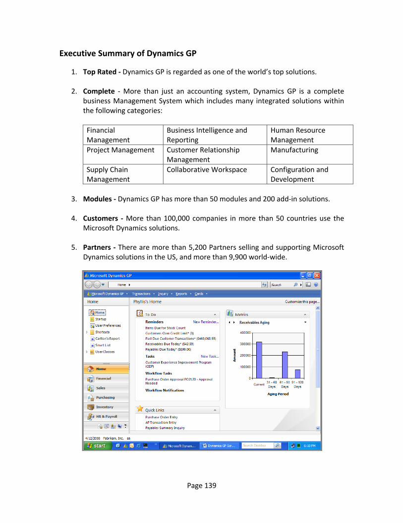
Page 139
Executive Summary of Dynamics GP
1. Top Rated ‐ Dynamics GP is regarded as one of the world’s top solutions.
2. Complete ‐ More than just an accounting system, Dynamics GP is a complete business Management System which includes many integrated solutions within the following categories:
Financial Management
Business Intelligence and Reporting
Human Resource Management
Project Management Customer Relationship Management
Manufacturing
Supply Chain Management
Collaborative Workspace Configuration and Development
3. Modules ‐ Dynamics GP has more than 50 modules and 200 add‐in solutions.
4. Customers ‐ More than 100,000 companies in more than 50 countries use the
Microsoft Dynamics solutions.
5. Partners ‐ There are more than 5,200 Partners selling and supporting Microsoft Dynamics solutions in the US, and more than 9,900 world‐wide.
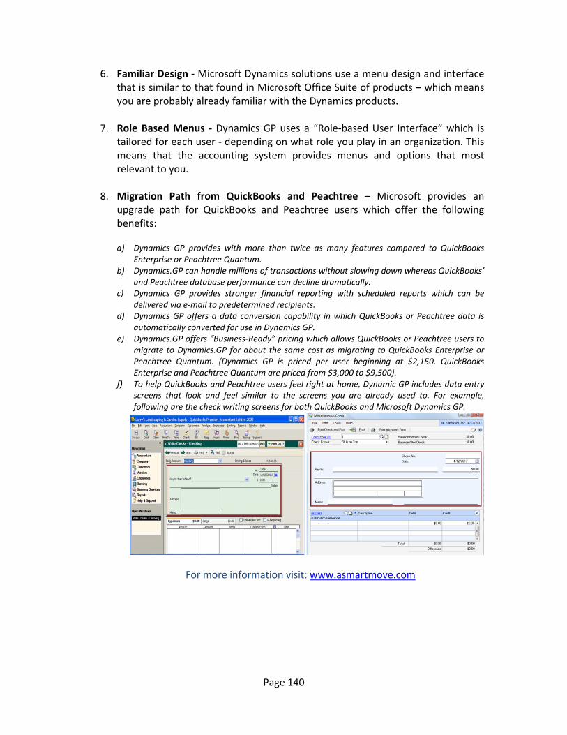
Page 140
6. Familiar Design ‐ Microsoft Dynamics solutions use a menu design and interface that is similar to that found in Microsoft Office Suite of products – which means you are probably already familiar with the Dynamics products.
7. Role Based Menus ‐ Dynamics GP uses a “Role‐based User Interface” which is tailored for each user ‐ depending on what role you play in an organization. This means that the accounting system provides menus and options that most relevant to you.
8. Migration Path from QuickBooks and Peachtree – Microsoft provides an upgrade path for QuickBooks and Peachtree users which offer the following benefits:
a) Dynamics GP provides with more than twice as many features compared to QuickBooks
Enterprise or Peachtree Quantum. b) Dynamics.GP can handle millions of transactions without slowing down whereas QuickBooks’
and Peachtree database performance can decline dramatically. c) Dynamics GP provides stronger financial reporting with scheduled reports which can be
delivered via e‐mail to predetermined recipients. d) Dynamics GP offers a data conversion capability in which QuickBooks or Peachtree data is
automatically converted for use in Dynamics GP. e) Dynamics.GP offers “Business‐Ready” pricing which allows QuickBooks or Peachtree users to
migrate to Dynamics.GP for about the same cost as migrating to QuickBooks Enterprise or Peachtree Quantum. (Dynamics GP is priced per user beginning at $2,150. QuickBooks Enterprise and Peachtree Quantum are priced from $3,000 to $9,500).
f) To help QuickBooks and Peachtree users feel right at home, Dynamic GP includes data entry screens that look and feel similar to the screens you are already used to. For example, following are the check writing screens for both QuickBooks and Microsoft Dynamics GP.
For more information visit: www.asmartmove.com
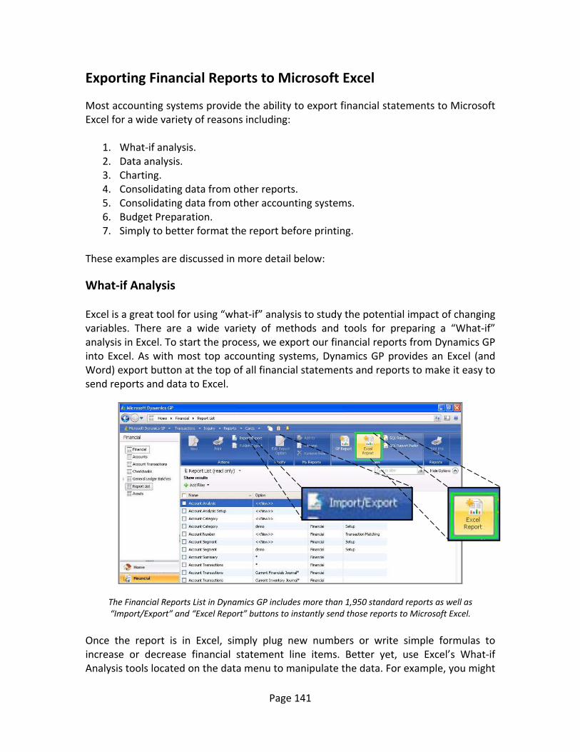
Page 141
Exporting Financial Reports to Microsoft Excel Most accounting systems provide the ability to export financial statements to Microsoft Excel for a wide variety of reasons including:
1. What‐if analysis. 2. Data analysis. 3. Charting. 4. Consolidating data from other reports. 5. Consolidating data from other accounting systems. 6. Budget Preparation. 7. Simply to better format the report before printing.
These examples are discussed in more detail below:
What‐if Analysis Excel is a great tool for using “what‐if” analysis to study the potential impact of changing variables. There are a wide variety of methods and tools for preparing a “What‐if” analysis in Excel. To start the process, we export our financial reports from Dynamics GP into Excel. As with most top accounting systems, Dynamics GP provides an Excel (and Word) export button at the top of all financial statements and reports to make it easy to send reports and data to Excel.
The Financial Reports List in Dynamics GP includes more than 1,950 standard reports as well as “Import/Export” and “Excel Report” buttons to instantly send those reports to Microsoft Excel.
Once the report is in Excel, simply plug new numbers or write simple formulas to increase or decrease financial statement line items. Better yet, use Excel’s What‐if Analysis tools located on the data menu to manipulate the data. For example, you might
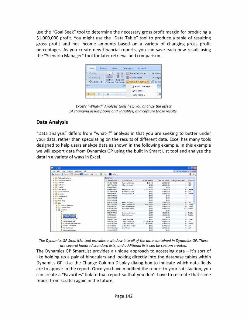
Page 142
use the “Goal Seek” tool to determine the necessary gross profit margin for producing a $1,000,000 profit. You might use the “Data Table” tool to produce a table of resulting gross profit and net income amounts based on a variety of changing gross profit percentages. As you create new financial reports, you can save each new result using the “Scenario Manager” tool for later retrieval and comparison.
Excel’s “What‐if” Analysis tools help you analyze the affect of changing assumptions and variables, and capture those results.
Data Analysis “Data analysis” differs from “what‐if” analysis in that you are seeking to better under your data, rather than speculating on the results of different data. Excel has many tools designed to help users analyze data as shown in the following example. In this example we will export data from Dynamics GP using the built in Smart List tool and analyze the data in a variety of ways in Excel.
The Dynamics GP SmartList tool provides a window into all of the data contained in Dynamics GP. There are several hundred standard lists, and additional lists can be custom created.
The Dynamics GP SmartList provides a unique approach to accessing data – it’s sort of like holding up a pair of binoculars and looking directly into the database tables within Dynamics GP. Use the Change Column Display dialog box to indicate which data fields are to appear in the report. Once you have modified the report to your satisfaction, you can create a “Favorites” link to that report so that you don’t have to recreate that same report from scratch again in the future.

Page 143
The Dynamics GP SmartList provides access to all data in the Dynamics GP database tables. As shown above, additional fields can be added to the reports, and filters can be applied to produce specific results. Additional SmartList features allow you to link to Microsoft Dynamics GP data from Office applications, using smart tags to speed access to customer, vendor, inventory, general ledger account, and employee information. For example, using the SmartList Builder, you can link data from Microsoft Dynamic GP to create a customized list of the information you want to review and analyze; then easily export inquiries to Word or Microsoft Office Excel for use in mass mailings or further analysis. You can view a complete listing of all standard SmartList reports here: http://www.microsoft.com/dynamics/gp/using/defaultsmartlistfavorites.mspx.
Simply click the Excel export tool located at the top of the SmartList to send the data to Excel.
The resulting data is exported to Excel as shown below. The Dynamcis GP SmartList export works well with Excel 2007 or previous versions of Excel if that is what is loaded on your computer.
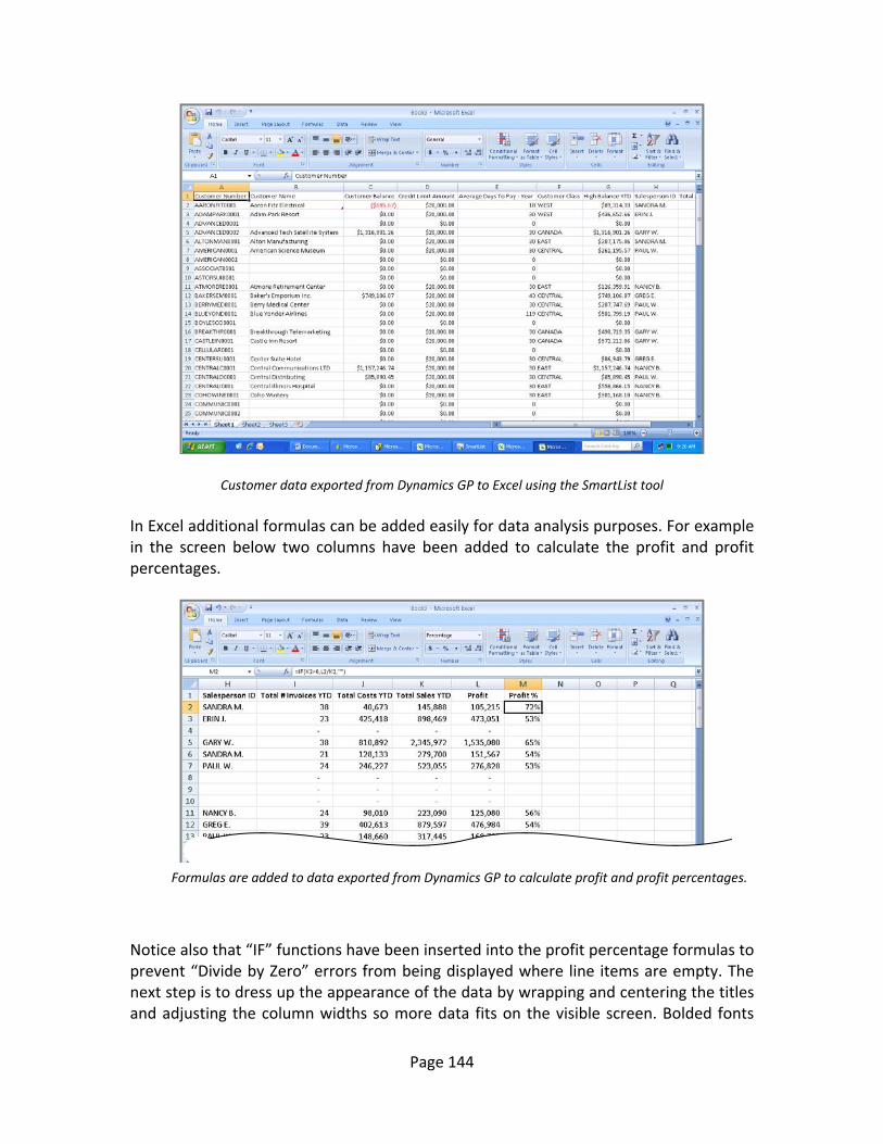
Page 144
Customer data exported from Dynamics GP to Excel using the SmartList tool
In Excel additional formulas can be added easily for data analysis purposes. For example in the screen below two columns have been added to calculate the profit and profit percentages.
Notice also that “IF” functions have been inserted into the profit percentage formulas to prevent “Divide by Zero” errors from being displayed where line items are empty. The next step is to dress up the appearance of the data by wrapping and centering the titles and adjusting the column widths so more data fits on the visible screen. Bolded fonts
Formulas are added to data exported from Dynamics GP to calculate profit and profit percentages.
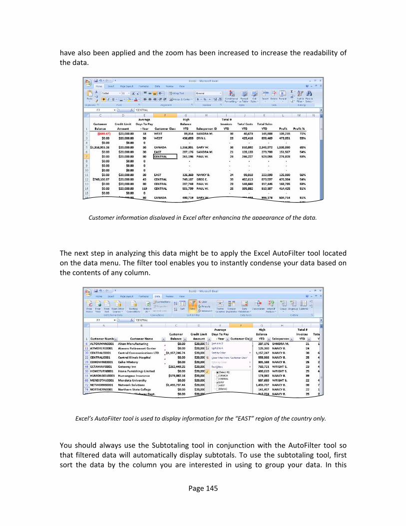
Page 145
have also been applied and the zoom has been increased to increase the readability of the data.
The next step in analyzing this data might be to apply the Excel AutoFilter tool located on the data menu. The filter tool enables you to instantly condense your data based on the contents of any column.
You should always use the Subtotaling tool in conjunction with the AutoFilter tool so that filtered data will automatically display subtotals. To use the subtotaling tool, first sort the data by the column you are interested in using to group your data. In this
Customer information displayed in Excel after enhancing the appearance of the data.
Excel’s AutoFilter tool is used to display information for the “EAST” region of the country only.
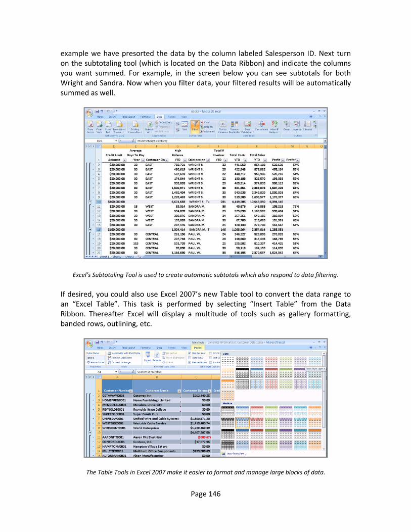
Page 146
example we have presorted the data by the column labeled Salesperson ID. Next turn on the subtotaling tool (which is located on the Data Ribbon) and indicate the columns you want summed. For example, in the screen below you can see subtotals for both Wright and Sandra. Now when you filter data, your filtered results will be automatically summed as well.
Excel’s Subtotaling Tool is used to create automatic subtotals which also respond to data filtering. If desired, you could also use Excel 2007’s new Table tool to convert the data range to an “Excel Table”. This task is performed by selecting “Insert Table” from the Data Ribbon. Thereafter Excel will display a multitude of tools such as gallery formatting, banded rows, outlining, etc.
The Table Tools in Excel 2007 make it easier to format and manage large blocks of data.
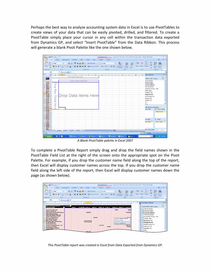
Page 147
Perhaps the best way to analyze accounting system data in Excel is to use PivotTables to create views of your data that can be easily pivoted, drilled, and filtered. To create a PivotTable simply place your cursor in any cell within the transaction data exported from Dynamics GP, and select “Insert PivotTable” from the Data Ribbon. This process will generate a blank Pivot Palette like the one shown below.
A Blank PivotTable palette in Excel 2007
To complete a PivotTable Report simply drag and drop the field names shown in the PivotTable Field List at the right of the screen onto the appropriate spot on the Pivot Palette. For example, if you drop the customer name field along the top of the report, then Excel will display customer names across the top. If you drop the customer name field along the left side of the report, then Excel will display customer names down the page (as shown below).
This PivotTable report was created in Excel from Data Exported from Dynamics GP.

Page 148
The next step might be to filter the data to display only those line items that show a balance in the “Balance Due” column. Perform this task by right clicking on the “Customer Name” title in the PivotTable and choose “Filter By Values” to create a filter rule to display only those line items where the balance due is greater than zero. This data can then be sorted by any column simply by placing the cursor in the desired column and choosing “Sort A to Z” or “Sort Z to A” from the “Data Ribbon”.
A PivotTable Report which has been filtered to suppress display of line items with a zero balance.
You might further filter the PivotTable Report to display selected data by column. For example, in the screen below we have filtered by salesperson ID to display the data for Greg, Nancy, Paul and Sandra only.
PivotTable Report filtered further by Column to display data only selected Salespersons.
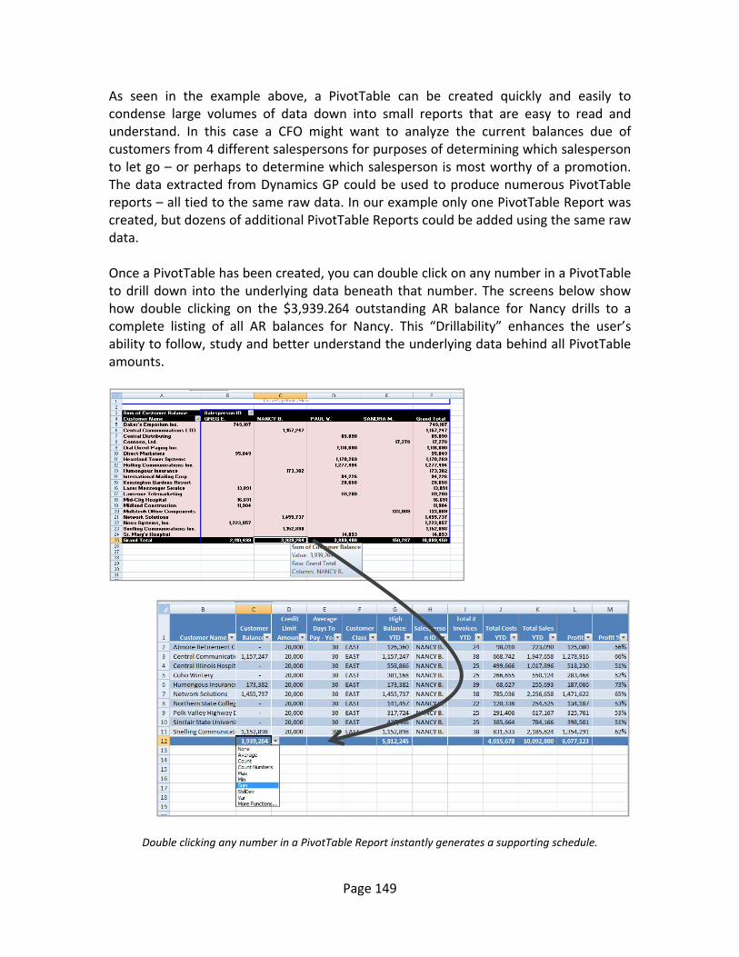
Page 149
As seen in the example above, a PivotTable can be created quickly and easily to condense large volumes of data down into small reports that are easy to read and understand. In this case a CFO might want to analyze the current balances due of customers from 4 different salespersons for purposes of determining which salesperson to let go – or perhaps to determine which salesperson is most worthy of a promotion. The data extracted from Dynamics GP could be used to produce numerous PivotTable reports – all tied to the same raw data. In our example only one PivotTable Report was created, but dozens of additional PivotTable Reports could be added using the same raw data. Once a PivotTable has been created, you can double click on any number in a PivotTable to drill down into the underlying data beneath that number. The screens below show how double clicking on the $3,939.264 outstanding AR balance for Nancy drills to a complete listing of all AR balances for Nancy. This “Drillability” enhances the user’s ability to follow, study and better understand the underlying data behind all PivotTable amounts.
Double clicking any number in a PivotTable Report instantly generates a supporting schedule.
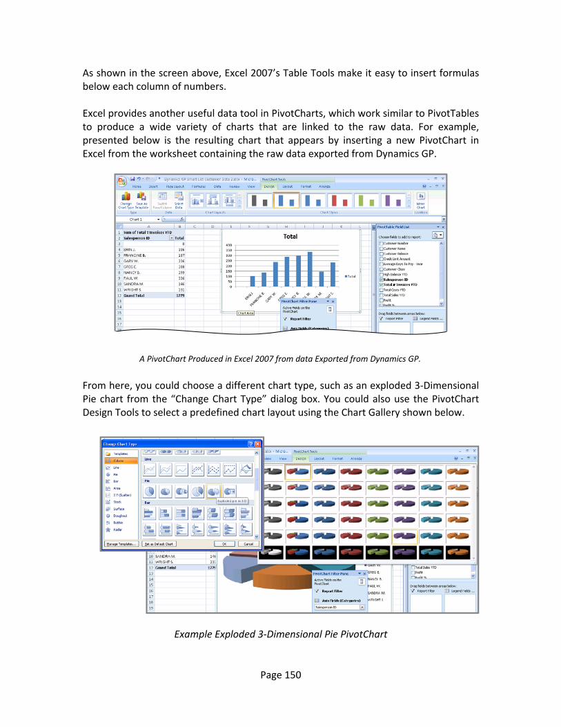
Page 150
As shown in the screen above, Excel 2007’s Table Tools make it easy to insert formulas below each column of numbers. Excel provides another useful data tool in PivotCharts, which work similar to PivotTables to produce a wide variety of charts that are linked to the raw data. For example, presented below is the resulting chart that appears by inserting a new PivotChart in Excel from the worksheet containing the raw data exported from Dynamics GP.
From here, you could choose a different chart type, such as an exploded 3‐Dimensional Pie chart from the “Change Chart Type” dialog box. You could also use the PivotChart Design Tools to select a predefined chart layout using the Chart Gallery shown below.
Example Exploded 3‐Dimensional Pie PivotChart
A PivotChart Produced in Excel 2007 from data Exported from Dynamics GP.
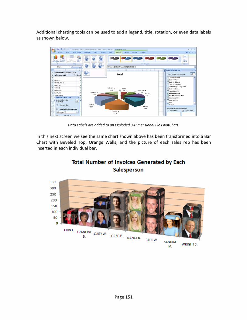
Page 151
Additional charting tools can be used to add a legend, title, rotation, or even data labels as shown below.
Data Labels are added to an Exploded 3‐Dimensional Pie PivotChart.
In this next screen we see the same chart shown above has been transformed into a Bar Chart with Beveled Top, Orange Walls, and the picture of each sales rep has been inserted in each individual bar.

Page 152
Automating the Task of Exporting Data Of course the idea of export and manipulating data each day, week, month quarter or year does not appeal to most CPAs because there is usually so much labor involved in the whole process. However this is not the case with some accounting systems. In Dynamics GP there are several methods for extracting the same data each day, week, month, quarter or year with a simple click of a button and the resulting data is sent to Excel where the PivotTables, PivotCharts, and reports you have already created are instantly linked to the new data, or are linked to the new data via a simple copy paste procedure. Listed below are five different approaches for automating the task of sending data to Excel from within Dynamics GP; each method has merit.
1. Dynamics GP SmartList Builder and Export Solution. 2. Dynamics GP Macro Recorder. 3. Excel ODBC Driver for Dynamics GP. 4. Excel OLAP Data Cubing. 5. Dynamics GP Dashboard Reporting.
As an example, the Dynamics GP SmartList Builder and Export Solution screen is shown below. This dialog box can be used to create data queries which are automatically generated in Dynamics GP and sent to Excel merely by clicking on the icon shown in the Export Box below. As you can see in the “Document Field” below, this export is already linked to the appropriate Excel workbook, and a simple double click in Dynamics GP updates the workbook with fresh data.
The Dynamics GP Export Solution Dialog Box helps Automate the Task of Sending Data to Excel Another option for sending data to Excel is the Dynamics GP Macro Recorder which works just like the macro recorder in Microsoft Excel. Simply select “Record a Macro” from the Dynamics GP menu, provide a name for the macro, and then export your data. When you are done exporting your data, simply select “Stop Recording” from the Dynamics GP menu and the macro is completed. Next time, simply run the macro and
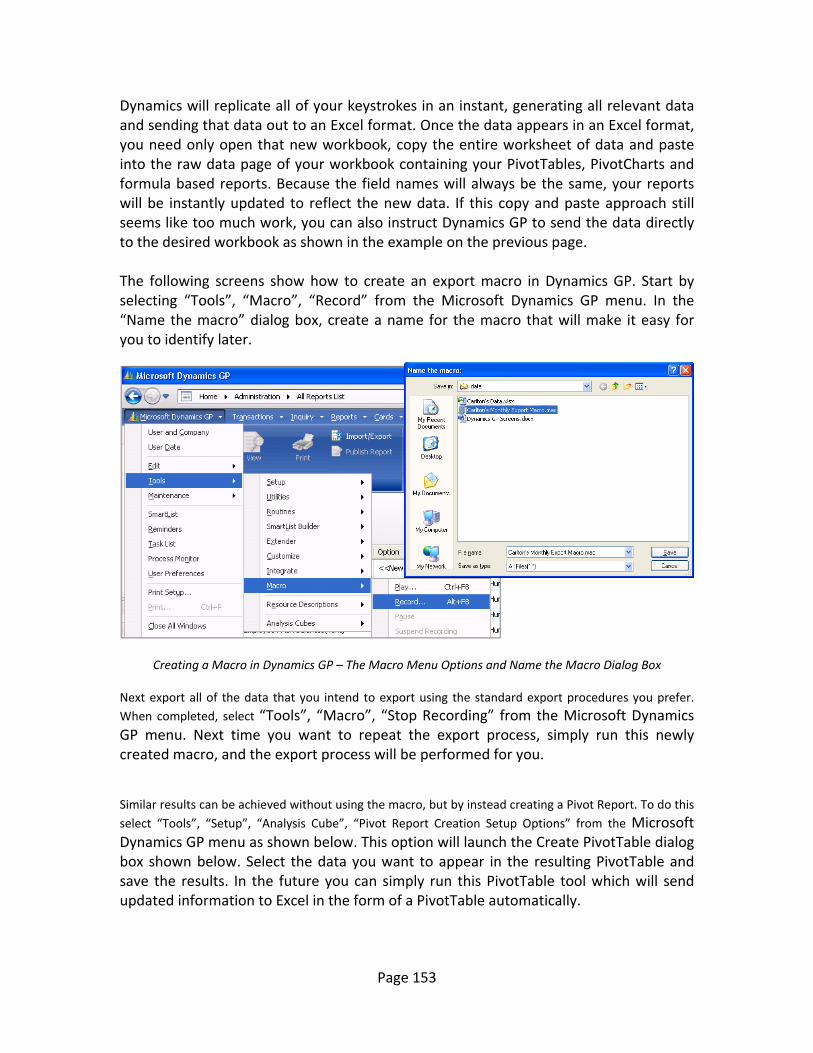
Page 153
Dynamics will replicate all of your keystrokes in an instant, generating all relevant data and sending that data out to an Excel format. Once the data appears in an Excel format, you need only open that new workbook, copy the entire worksheet of data and paste into the raw data page of your workbook containing your PivotTables, PivotCharts and formula based reports. Because the field names will always be the same, your reports will be instantly updated to reflect the new data. If this copy and paste approach still seems like too much work, you can also instruct Dynamics GP to send the data directly to the desired workbook as shown in the example on the previous page. The following screens show how to create an export macro in Dynamics GP. Start by selecting “Tools”, “Macro”, “Record” from the Microsoft Dynamics GP menu. In the “Name the macro” dialog box, create a name for the macro that will make it easy for you to identify later.
Creating a Macro in Dynamics GP – The Macro Menu Options and Name the Macro Dialog Box Next export all of the data that you intend to export using the standard export procedures you prefer. When completed, select “Tools”, “Macro”, “Stop Recording” from the Microsoft Dynamics GP menu. Next time you want to repeat the export process, simply run this newly created macro, and the export process will be performed for you. Similar results can be achieved without using the macro, but by instead creating a Pivot Report. To do this select “Tools”, “Setup”, “Analysis Cube”, “Pivot Report Creation Setup Options” from the Microsoft Dynamics GP menu as shown below. This option will launch the Create PivotTable dialog box shown below. Select the data you want to appear in the resulting PivotTable and save the results. In the future you can simply run this PivotTable tool which will send updated information to Excel in the form of a PivotTable automatically.
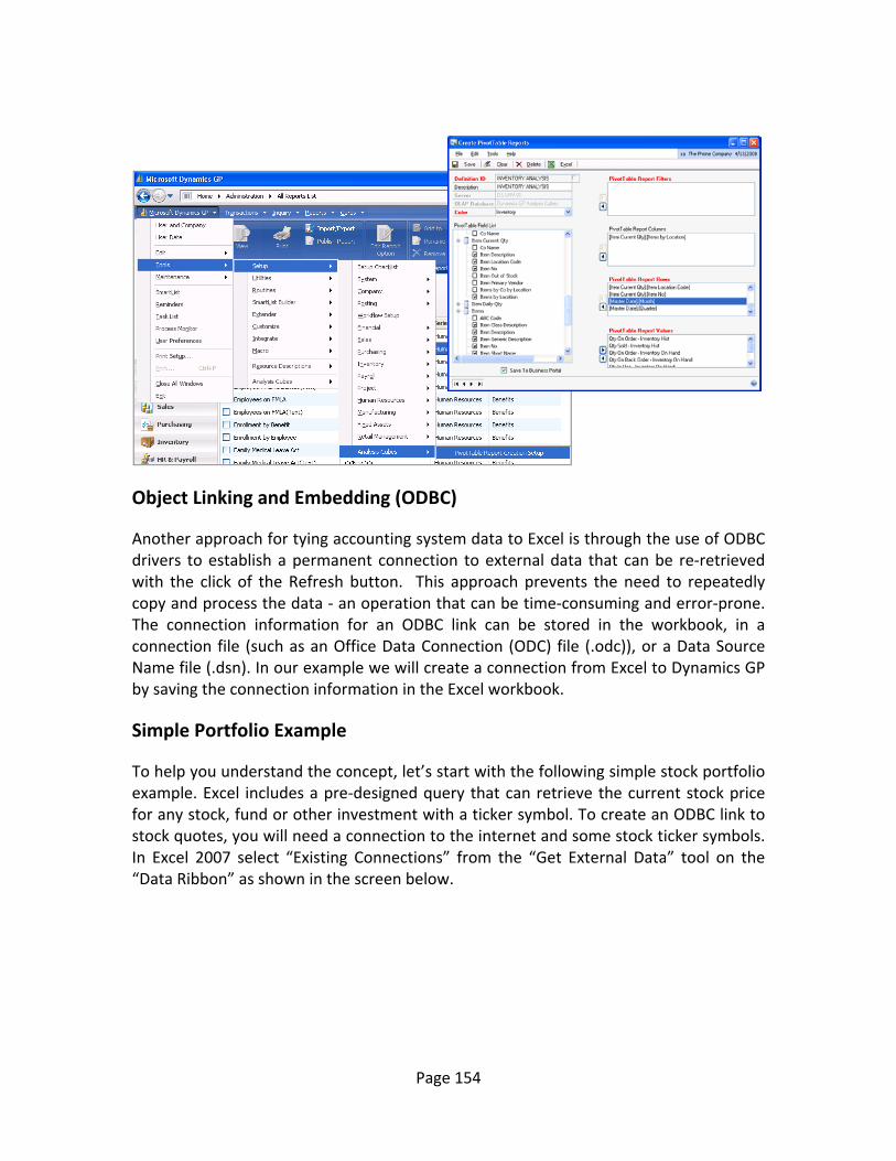
Page 154
Object Linking and Embedding (ODBC) Another approach for tying accounting system data to Excel is through the use of ODBC drivers to establish a permanent connection to external data that can be re‐retrieved with the click of the Refresh button. This approach prevents the need to repeatedly copy and process the data ‐ an operation that can be time‐consuming and error‐prone. The connection information for an ODBC link can be stored in the workbook, in a connection file (such as an Office Data Connection (ODC) file (.odc)), or a Data Source Name file (.dsn). In our example we will create a connection from Excel to Dynamics GP by saving the connection information in the Excel workbook.
Simple Portfolio Example To help you understand the concept, let’s start with the following simple stock portfolio example. Excel includes a pre‐designed query that can retrieve the current stock price for any stock, fund or other investment with a ticker symbol. To create an ODBC link to stock quotes, you will need a connection to the internet and some stock ticker symbols. In Excel 2007 select “Existing Connections” from the “Get External Data” tool on the “Data Ribbon” as shown in the screen below.

Page 155
The “Existing Connections” dialog box will appear. Double‐click the option for “MSN MoneyCentral Investor Stock Quotes” as shown below.
Next the “Import Data” wizard (shown below) will appear to walk you through the data connection process. Click OK in the first dialog box and in the second dialog box enter the ticker symbols you are interested in separated by commas, and check the box titled “use this value for future refreshes”. Here I have entered ticker symbols for Microsoft, Coca‐Cola, Google, Intel and Apple Computers.
Press OK to complete the data connection. The following information will be displayed in Excel.
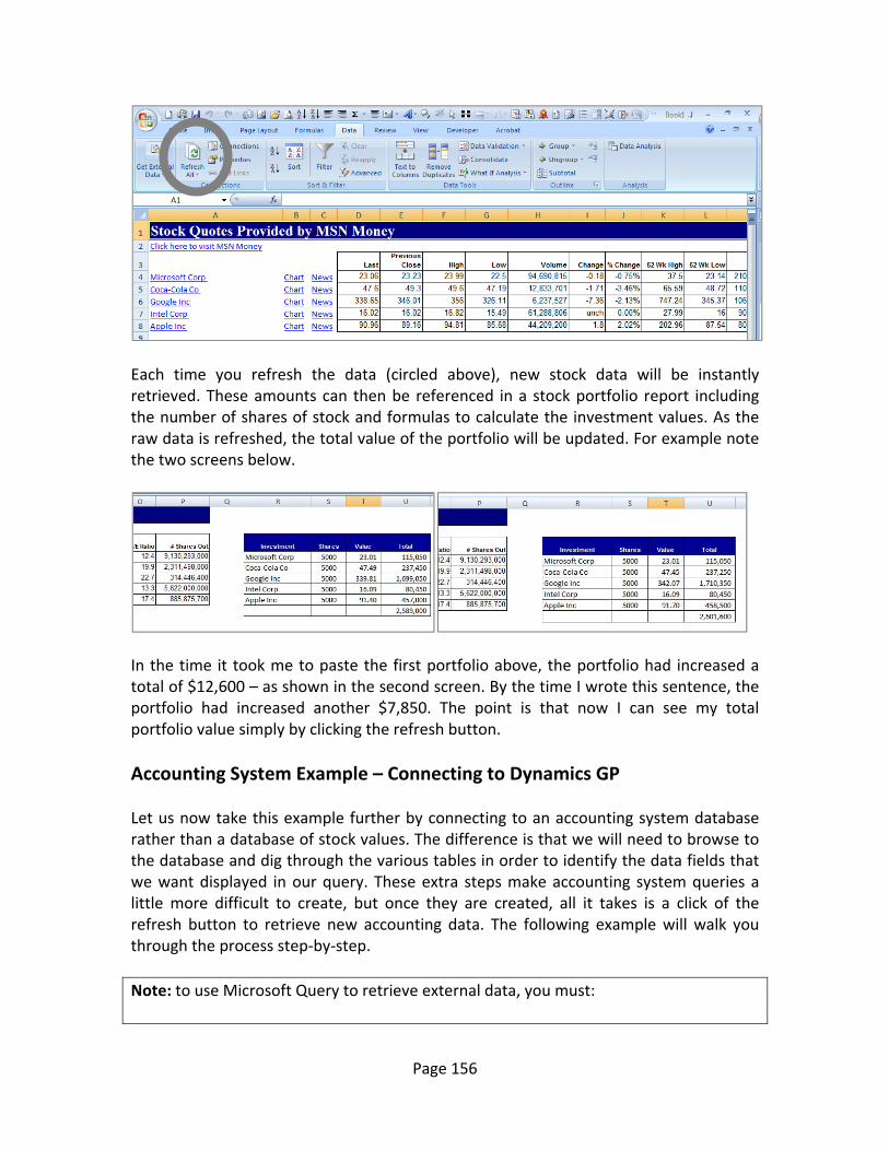
Page 156
Each time you refresh the data (circled above), new stock data will be instantly retrieved. These amounts can then be referenced in a stock portfolio report including the number of shares of stock and formulas to calculate the investment values. As the raw data is refreshed, the total value of the portfolio will be updated. For example note the two screens below.
In the time it took me to paste the first portfolio above, the portfolio had increased a total of $12,600 – as shown in the second screen. By the time I wrote this sentence, the portfolio had increased another $7,850. The point is that now I can see my total portfolio value simply by clicking the refresh button. Accounting System Example – Connecting to Dynamics GP Let us now take this example further by connecting to an accounting system database rather than a database of stock values. The difference is that we will need to browse to the database and dig through the various tables in order to identify the data fields that we want displayed in our query. These extra steps make accounting system queries a little more difficult to create, but once they are created, all it takes is a click of the refresh button to retrieve new accounting data. The following example will walk you through the process step‐by‐step. Note: to use Microsoft Query to retrieve external data, you must:
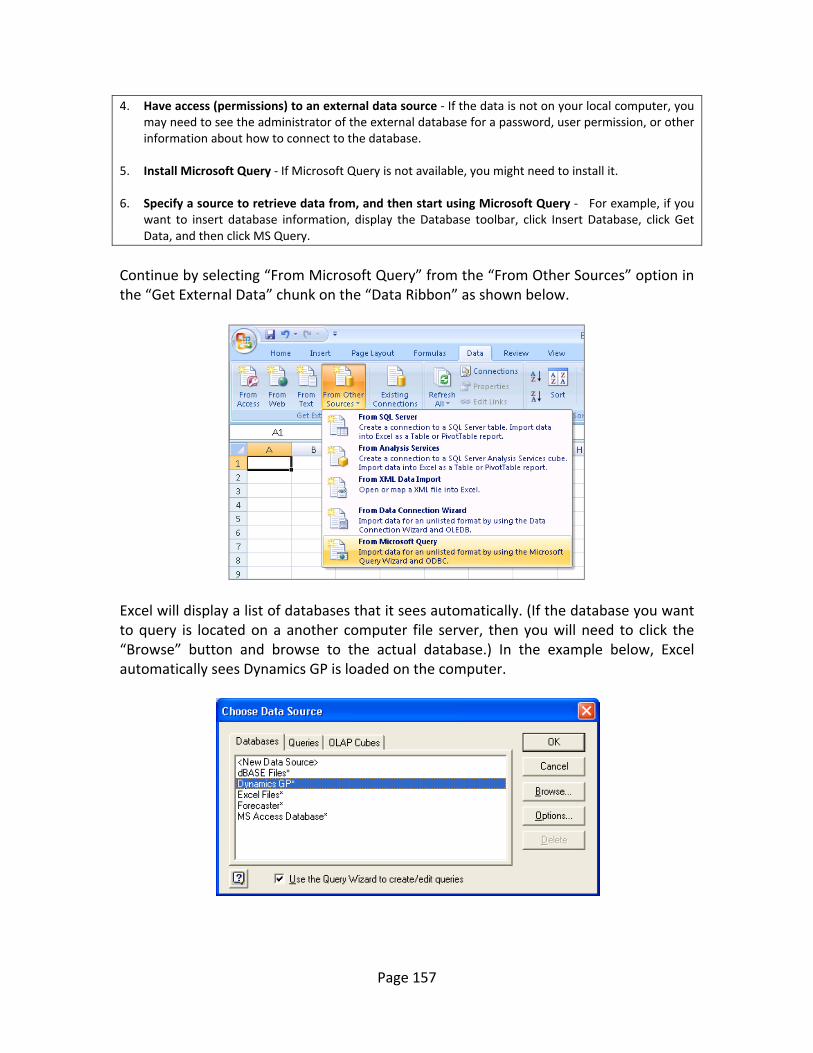
Page 157
4. Have access (permissions) to an external data source ‐ If the data is not on your local computer, you may need to see the administrator of the external database for a password, user permission, or other information about how to connect to the database.
5. Install Microsoft Query ‐ If Microsoft Query is not available, you might need to install it. 6. Specify a source to retrieve data from, and then start using Microsoft Query ‐ For example, if you
want to insert database information, display the Database toolbar, click Insert Database, click Get Data, and then click MS Query.
Continue by selecting “From Microsoft Query” from the “From Other Sources” option in the “Get External Data” chunk on the “Data Ribbon” as shown below.
Excel will display a list of databases that it sees automatically. (If the database you want to query is located on a another computer file server, then you will need to click the “Browse” button and browse to the actual database.) In the example below, Excel automatically sees Dynamics GP is loaded on the computer.

Page 158
Select the Dynamics GP option and login to the database as shown below. Note that ODBC connections and web queries obey all database permissions; therefore a password is typically needed to create this type of connection.
Upon logging in, the Excel Query wizard will display a list of table names. Scroll through the list and find the table that contains the data you want. This is usually the hardest part of the process because it can be difficult to know exactly which table contains the data you are after. However with a little bit of effort, trial and error search, and perhaps a sense of humor, eventually you will find data you are after.
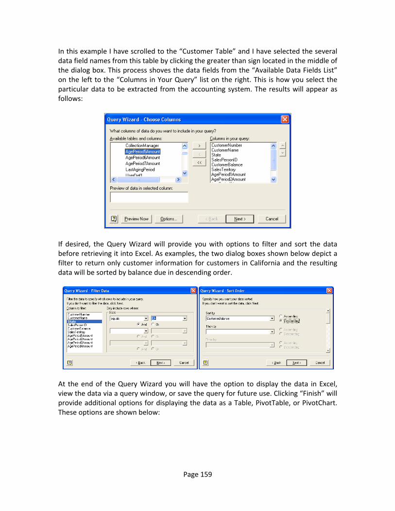
Page 159
In this example I have scrolled to the “Customer Table” and I have selected the several data field names from this table by clicking the greater than sign located in the middle of the dialog box. This process shoves the data fields from the “Available Data Fields List” on the left to the “Columns in Your Query” list on the right. This is how you select the particular data to be extracted from the accounting system. The results will appear as follows:
If desired, the Query Wizard will provide you with options to filter and sort the data before retrieving it into Excel. As examples, the two dialog boxes shown below depict a filter to return only customer information for customers in California and the resulting data will be sorted by balance due in descending order.
At the end of the Query Wizard you will have the option to display the data in Excel, view the data via a query window, or save the query for future use. Clicking “Finish” will provide additional options for displaying the data as a Table, PivotTable, or PivotChart. These options are shown below:
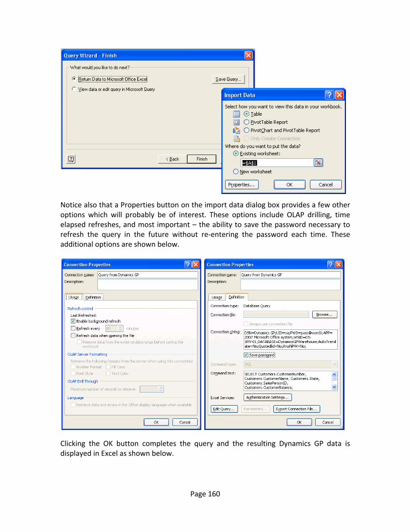
Page 160
Notice also that a Properties button on the import data dialog box provides a few other options which will probably be of interest. These options include OLAP drilling, time elapsed refreshes, and most important – the ability to save the password necessary to refresh the query in the future without re‐entering the password each time. These additional options are shown below.
Clicking the OK button completes the query and the resulting Dynamics GP data is displayed in Excel as shown below.
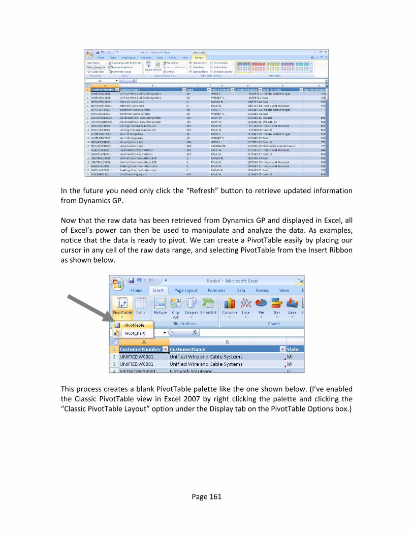
Page 161
In the future you need only click the “Refresh” button to retrieve updated information from Dynamics GP. Now that the raw data has been retrieved from Dynamics GP and displayed in Excel, all of Excel’s power can then be used to manipulate and analyze the data. As examples, notice that the data is ready to pivot. We can create a PivotTable easily by placing our cursor in any cell of the raw data range, and selecting PivotTable from the Insert Ribbon as shown below.
This process creates a blank PivotTable palette like the one shown below. (I’ve enabled the Classic PivotTable view in Excel 2007 by right clicking the palette and clicking the “Classic PivotTable Layout” option under the Display tab on the PivotTable Options box.)

Page 162
Next I drag and drop the “CustomerName”, “CustomerBalance”, and “SalesPersonId” fields onto the palette to create the following PivotTable report.
Because some customer balances and salesperson balances are zero, I apply a “Value Filter” to show only those customers and salespersons with actual amounts due (that is amounts greater than Zero). I apply the same type of filter to the salesperson field as well.
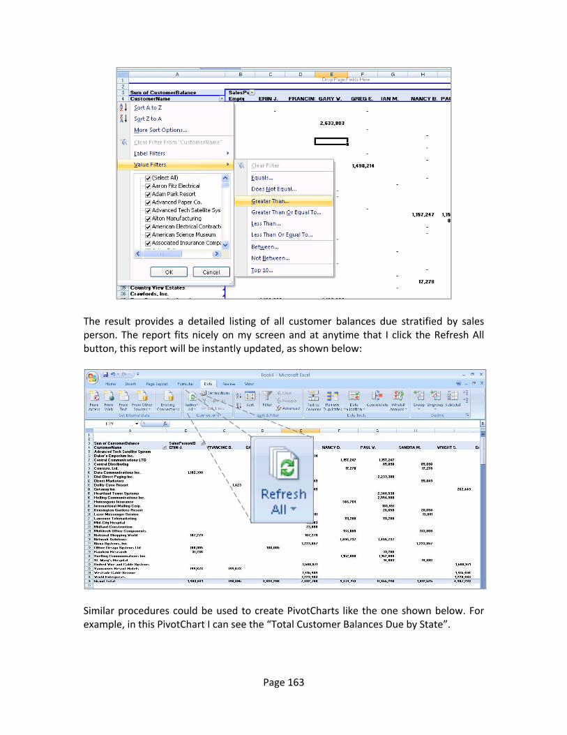
Page 163
The result provides a detailed listing of all customer balances due stratified by sales person. The report fits nicely on my screen and at anytime that I click the Refresh All button, this report will be instantly updated, as shown below:
Similar procedures could be used to create PivotCharts like the one shown below. For example, in this PivotChart I can see the “Total Customer Balances Due by State”.

Page 164
Analyzing Inventory in Excel As another example, let us apply the same ODBC techniques described above to analyze inventory. In this case we browse to the “Inventory Item Master Table” and retrieve the following information:
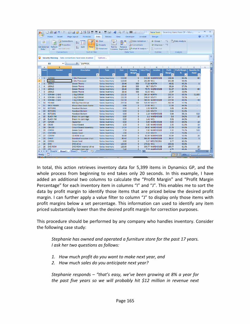
Page 165
In total, this action retrieves inventory data for 5,399 items in Dynamics GP, and the whole process from beginning to end takes only 20 seconds. In this example, I have added an additional two columns to calculate the “Profit Margin” and “Profit Margin Percentage” for each inventory item in columns “I” and “J”. This enables me to sort the data by profit margin to identify those items that are priced below the desired profit margin. I can further apply a value filter to column “J” to display only those items with profit margins below a set percentage. This information can used to identify any item priced substantially lower than the desired profit margin for correction purposes. This procedure should be performed by any company who handles inventory. Consider the following case study:
Stephanie has owned and operated a furniture store for the past 17 years. I ask her two questions as follows:
1. How much profit do you want to make next year, and 2. How much sales do you anticipate next year?
Stephanie responds – “that’s easy, we’ve been growing at 8% a year for the past five years so we will probably hit $12 million in revenue next

Page 166
year. Also, I’d like to make a million dollars profit – I think that’s a reasonable goal.
With just this little bit of data, we can work backwards based on Stephanie’s prior year financial statements and advise her as follows: “Stephanie your fixed costs are $2 million and you want to make another $1 million in profit. $3 million is 25% of your anticipated sales of $12 million, therefore you need to price your furniture with a 25% margin to achieve the desired results. Further analysis shows that Stephanie’s furniture is currently priced at just 22% margin, which works out to a potential profit of just $640,000. At this point we tell Stephanie the story about the good ole boys who were selling onions. It goes like this:
These two Florida boys were running up to Georgia and buying Vidalia onions at 4 for $1.00 which they then sold for a quarter a piece on the streets of Jacksonville. After six months, one boy turned to the other and said – “you know, I don’t think we’re making any money – what do you think we need to do different?” The other boy thought real hard and then blurted – “I think we need a bigger truck”.
OK, it’s an old story. Also, it’s an exaggerated story as well. But there is a lesson to be learned here. If you don’t price your products to make a profit, you will never make a profit. And, if you don’t price your products to make your desired profit, you will never make your desired profits. This “Target Profit Margin” is a rather easy calculation for any CPA to make – yet CPAs often fail to make this simple calculation. Still there is another issue in that fluctuating costs make it almost impossible to hit the targeted sales process unless you make daily price adjustments. This is where a strong accounting system will help.
In our example above, Stephanie should consider using the “Margin Pricing Option” in her accounting system to always adjust prices to reflect a profit margin of 25%. In this manner, if her costs go up or down, her price will adjust accordingly to provide the desired profit margin. The result is that Stephanie will then have the chance to achieve her goals. (There are of course, other factors at play that may prevent success, but without adequate pricing, Stephanie will have no chance at all of hitting her target ‐ think about it.) The screen below shows how margin pricing is applied in Dynamics GP.
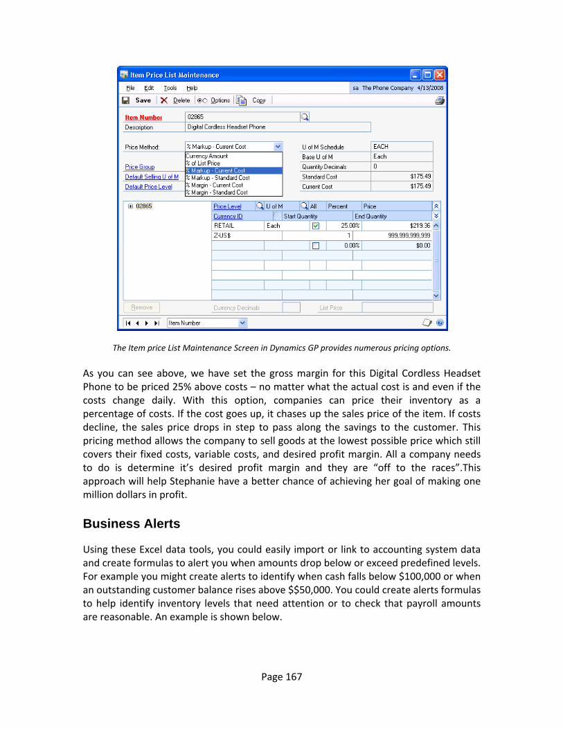
Page 167
The Item price List Maintenance Screen in Dynamics GP provides numerous pricing options.
As you can see above, we have set the gross margin for this Digital Cordless Headset Phone to be priced 25% above costs – no matter what the actual cost is and even if the costs change daily. With this option, companies can price their inventory as a percentage of costs. If the cost goes up, it chases up the sales price of the item. If costs decline, the sales price drops in step to pass along the savings to the customer. This pricing method allows the company to sell goods at the lowest possible price which still covers their fixed costs, variable costs, and desired profit margin. All a company needs to do is determine it’s desired profit margin and they are “off to the races”.This approach will help Stephanie have a better chance of achieving her goal of making one million dollars in profit. Business Alerts Using these Excel data tools, you could easily import or link to accounting system data and create formulas to alert you when amounts drop below or exceed predefined levels. For example you might create alerts to identify when cash falls below $100,000 or when an outstanding customer balance rises above $$50,000. You could create alerts formulas to help identify inventory levels that need attention or to check that payroll amounts are reasonable. An example is shown below.
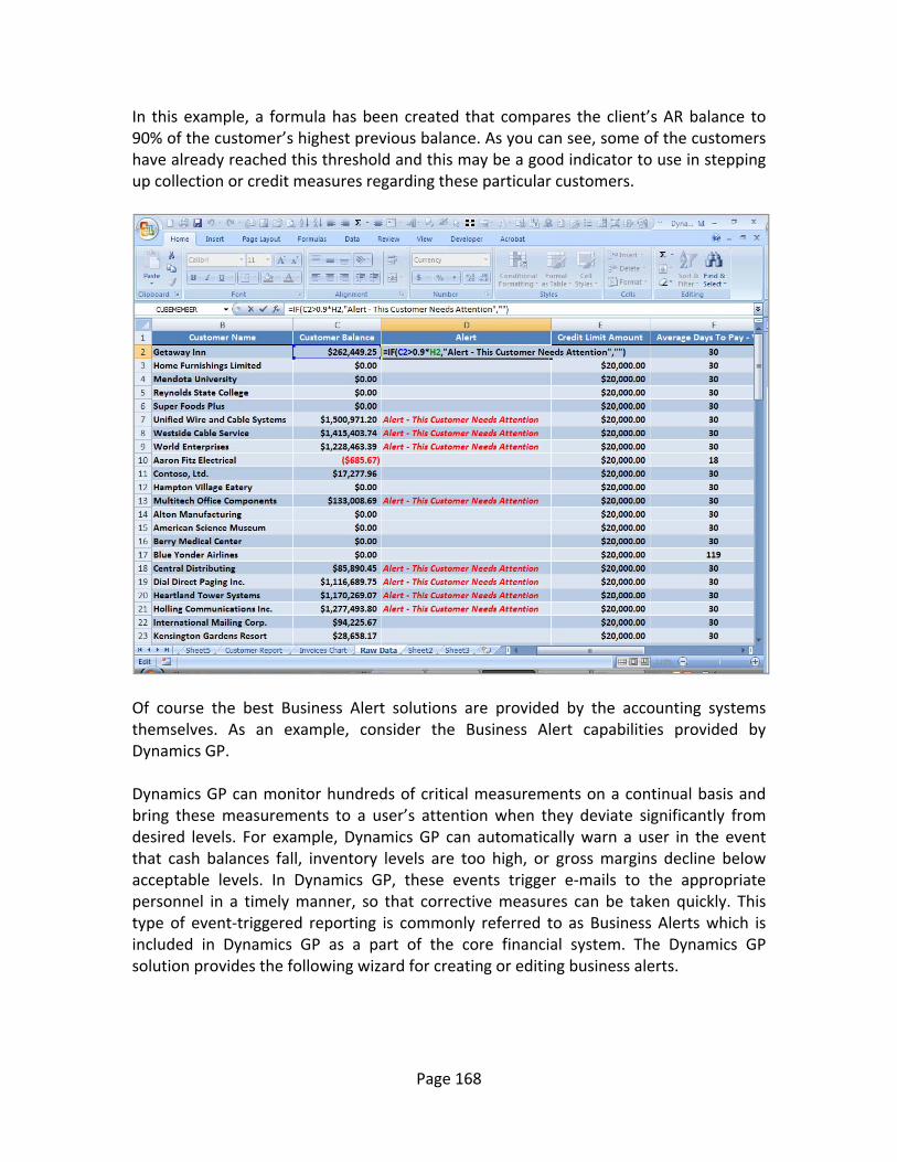
Page 168
In this example, a formula has been created that compares the client’s AR balance to 90% of the customer’s highest previous balance. As you can see, some of the customers have already reached this threshold and this may be a good indicator to use in stepping up collection or credit measures regarding these particular customers.
Of course the best Business Alert solutions are provided by the accounting systems themselves. As an example, consider the Business Alert capabilities provided by Dynamics GP. Dynamics GP can monitor hundreds of critical measurements on a continual basis and bring these measurements to a user’s attention when they deviate significantly from desired levels. For example, Dynamics GP can automatically warn a user in the event that cash balances fall, inventory levels are too high, or gross margins decline below acceptable levels. In Dynamics GP, these events trigger e‐mails to the appropriate personnel in a timely manner, so that corrective measures can be taken quickly. This type of event‐triggered reporting is commonly referred to as Business Alerts which is included in Dynamics GP as a part of the core financial system. The Dynamics GP solution provides the following wizard for creating or editing business alerts.

Page 169
Creating Budgets in Excel using Linear Regression Analysis Excel provides the ability to extrapolate data from your accounting system to produce budgets, projections or forecasts using the least squares method of linear regression analysis. The process is extremely easy as follows. In this example we start by exporting 3 years worth of monthly trial balance data from Dynamics GP to Microsoft Excel. In Dynamics we have printed the report to the screen and also to a comma separated value print file.
Dynamics GP Business Alerts provides a wizard for
creating complex calculations, scheduling
calculations, and reporting
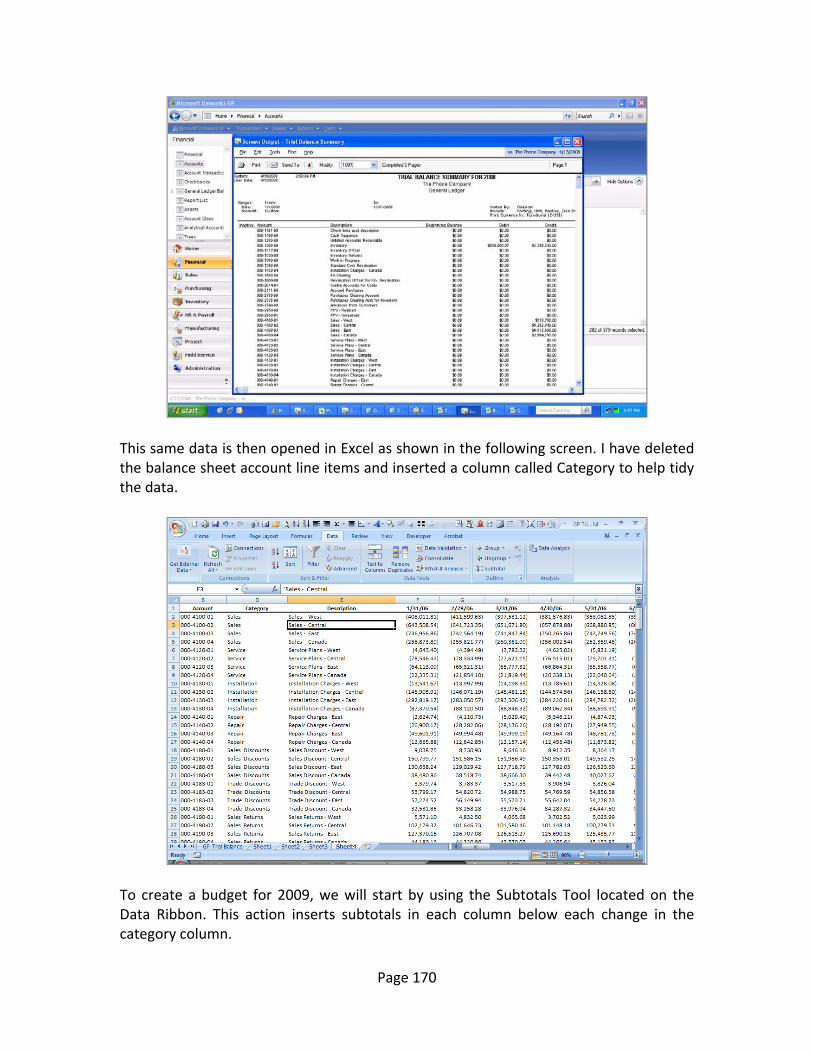
Page 170
This same data is then opened in Excel as shown in the following screen. I have deleted the balance sheet account line items and inserted a column called Category to help tidy the data.
To create a budget for 2009, we will start by using the Subtotals Tool located on the Data Ribbon. This action inserts subtotals in each column below each change in the category column.
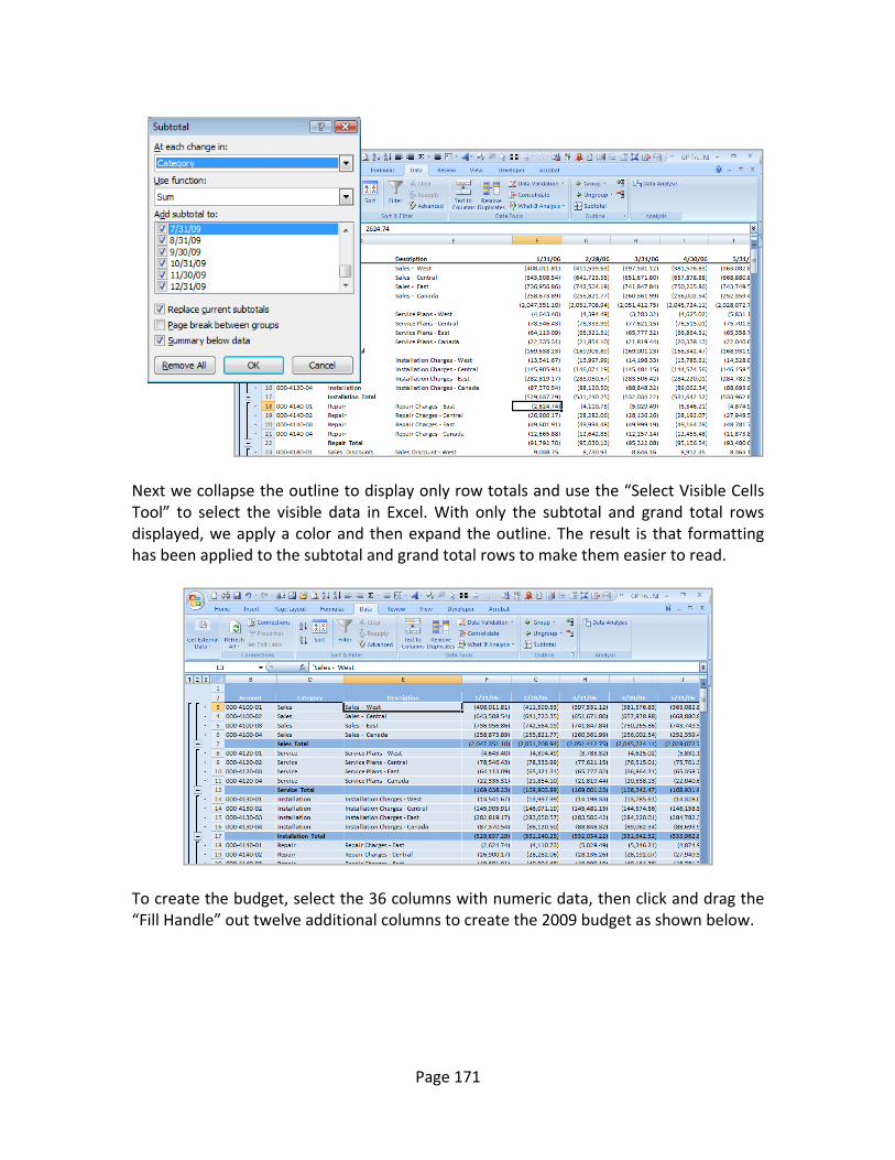
Page 171
Next we collapse the outline to display only row totals and use the “Select Visible Cells Tool” to select the visible data in Excel. With only the subtotal and grand total rows displayed, we apply a color and then expand the outline. The result is that formatting has been applied to the subtotal and grand total rows to make them easier to read.
To create the budget, select the 36 columns with numeric data, then click and drag the “Fill Handle” out twelve additional columns to create the 2009 budget as shown below.
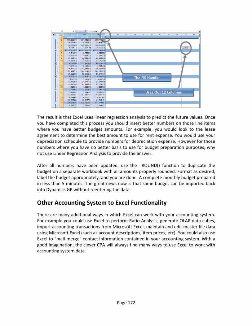
Page 172
The result is that Excel uses linear regression analysis to predict the future values. Once you have completed this process you should insert better numbers on those line items where you have better budget amounts. For example, you would look to the lease agreement to determine the best amount to use for rent expense. You would use your depreciation schedule to provide numbers for depreciation expense. However for those numbers where you have no better basis to use for budget preparation purposes, why not use Linear Regression Analysis to provide the answer. After all numbers have been updated, use the =ROUND() function to duplicate the budget on a separate workbook with all amounts properly rounded. Format as desired, label the budget appropriately, and you are done. A complete monthly budget prepared in less than 5 minutes. The great news now is that same budget can be imported back into Dynamics GP without reentering the data.
Other Accounting System to Excel Functionality There are many additional ways in which Excel can work with your accounting system. For example you could use Excel to perform Ratio Analysis, generate OLAP data cubes, import accounting transactions from Microsoft Excel, maintain and edit master file data using Microsoft Excel (such as account descriptions, item prices, etc). You could also use Excel to “mail‐merge” contact information contained in your accounting system. With a good imagination, the clever CPA will always find many ways to use Excel to work with accounting system data.
The Fill Handle
Drag Out 12 Columns

Page 173
Biography & Contact Information J. Carlton Collins, CPA , ASA Research, [email protected], 770.734.0950
J. Carlton Collins, CPA is a Certified Public Accountant with experience in technology, tax, auditing, accounting systems, financial reporting, and bond financing. He is an author, lecturer, and technology & accounting systems consultant. He has published more than two dozen books, two hundred articles, and thousands of web pages. As a public speaker, Mr. Collins has delivered more than 2,000 lectures in 44 states and 5 countries addressing more than 500,000 business professionals, including numerous keynote lectures at national and international conferences. Key awards include: "AICPA Lifetime Achievement Award", "Tom Radcliffe Outstanding Discussion Leader Award", "GSCPA Outstanding Discussion Leader Award", and "Accounting Technologies' Top Ten CPA Technologists Award". As a consultant, Mr. Collins has assisted 275+ large and small
companies with the selection and implementation of accounting systems. Mr. Collins has a Bachelors degree in Accounting from the University of Georgia, is a 27 year member of the AICPA and the Georgia Society of CPAs, and is also a licensed realtor. At the University of Georgia Mr. Collins was elected President of the Phi Eta Sigma Honor Society, was initiated into the BIFTAD Honor Society, was a member of Alpha Tau Omega fraternity, and served three years in the Judicial Defender/Advocate program. At Glynn Academy High School Mr. Collins was Senior Class President, Class Co‐Valedictorian, and received a principle nomination to Annapolis Naval Academy. Mr. Collins has been married for 25 years and has two children. He devotes his leisure time to family, travel, tennis, fishing, snow skiing, and riding motorcycles (dirt and street). Mr. Collins is president of his home owners association, participates in the Gwinnett Clean and Beautiful program, and volunteers for Cooperative Ministries food drive. He was a finalist in the 2009 South’s Funniest Accountant Competition which raises money for Junior Achievement. Selected Positions, Awards & Accomplishments:
1. 2008 and 2009 Chairman of the Southeast Accounting Show ‐ the south's largest CPA event. 2. Recipient of the 2008 Tom Radcliff Outstanding Discussion Leader Award. 3. Named “Top Ten CPA Technologists” by Accounting Technologies Magazine; Named “Top 100 Most
Influential CPAs ” by Accounting Technologies Magazine in multiple years. 4. Has personally delivered over 1,500 technology lectures around the world. 5. Has published 80+ pages of accounting software articles in the Journal of Accountancy. 6. Recipient of the AICPA Lifetime Technical Contribution to the CPA Profession Award. 7. Recipient of the Outstanding Discussion Leader Award from the Georgia Society of CPAs. 8. Lead author for PPC's Guide to Installing Microcomputer Accounting Systems. 9. Has installed accounting systems for more than 200 companies. 10. Past Chairperson of the AICPA Technology Conference. 11. Has delivered keynote and session lectures at dozens of accounting software conferences including seven
Microsoft Partner Conferences, five Sage Conferences, and multiple conferences for Epicor, Open Systems, Exact Software, Sage ACCPAC ERP, Dynamics.NAV, Dynamics. AX, SouthWare, Axapta .
12. Has provided consulting services to many computer companies (including Compaq, IBM, Microsoft, Apple, Novell, Peachtree, Epicor, Sage Software, Exact, ACCPAC, Intuit, Peachtree, Great Plains, and others).
As an auditor Mr. Collins has audited businesses in the areas of health care, construction, distribution, automobile dealerships, insurance, manufacturing, and general business. Mr. Collins' tax experience includes corporate, individual, partnership, fiduciary, and estate tax planning work. In the area of finance, Mr. Collins has prepared feasibility studies and financial forecasts for nearly 300 projects seeking more than $3 billion in startup capital, including field work for 80 of those projects. Mr. Collins is familiar with bond issues, Medicare and Medicaid reimbursement, and conventional financing matters. As a consultant, Mr. Collins worked with the entire Microsoft Excel development team contributing more than 500 pages of design improvements ‐ many of which are found in Excel today.

Page 174
This page intentionally blank
Page 175