arX

iv:h

ep-t

h/00

0717

0v3

24

Aug

200

0

D–Brane Primer

Clifford V. Johnson

Department of Mathematical SciencesScience Laboratories, South Road

Durham DH1 3LEEngland, U.K.

c.v.johnson@durham.ac.uk

Following is a collection of lecture notes on D–branes, which may be used by thereader as preparation for applications to modern research applications such as:the AdS/CFT and other gauge theory/geometry correspondences, Matrix The-ory and stringy non–commutative geometry, etc. In attempting to be reasonablyself–contained, the notes start from classical point–particles and develop the sub-ject logically (but selectively) through classical strings, quantisation, D–branes,supergravity, superstrings, string duality, including many detailed applications.Selected focus topics feature D–branes as probes of both spacetime and gaugegeometry, highlighting the role of world–volume curvature and gauge couplings,with some non–Abelian cases. Other advanced topics which are discussed are the(presently) novel tools of research such as fractional branes, the enhancon mecha-nism, D(ielectric)–branes and the emergence of the fuzzy/non–commutative sphere.(This is an expanded writeup of lectures given at ICTP, TASI, and BUSSTEPP.)

Contents

1 Opening Remarks 4

2 String Worldsheet Perspective, Mostly 72.1 Classical Point Particles . . . . . . . . . . . . . . . . . . . . . . 72.2 Classical Bosonic Strings . . . . . . . . . . . . . . . . . . . . . . 92.3 Quantised Bosonic Strings . . . . . . . . . . . . . . . . . . . . . 232.4 Chan-Paton Factors . . . . . . . . . . . . . . . . . . . . . . . . 332.5 The Closed String Partition Function . . . . . . . . . . . . . . . 342.6 Unoriented Strings . . . . . . . . . . . . . . . . . . . . . . . . . 392.7 Strings in Curved Backgrounds . . . . . . . . . . . . . . . . . . 43

3 Target Spacetime Perspective, Mostly 473.1 T–Duality for Closed Strings . . . . . . . . . . . . . . . . . . . 473.2 The Circle Partition Function . . . . . . . . . . . . . . . . . . . 513.3 Self–Duality and Enhanced Gauge Symmetry . . . . . . . . . . 52

1

3.4 T–duality in Background Fields . . . . . . . . . . . . . . . . . . 543.5 Another Special Radius: Bosonisation . . . . . . . . . . . . . . 553.6 String Theory on an Orbifold . . . . . . . . . . . . . . . . . . . 583.7 T–Duality for Open Strings: D–branes . . . . . . . . . . . . . . 613.8 D–Brane Dynamics: Collective Coords and Gauge Theory . . . 633.9 T–Duality and Orientifolds. . . . . . . . . . . . . . . . . . . . . 673.10 The D–Brane Tension . . . . . . . . . . . . . . . . . . . . . . . 703.11 The Orientifold Tension . . . . . . . . . . . . . . . . . . . . . . 75

4 Worldvolume Actions I: Dirac–Born–Infeld 774.1 Tilted D–Branes . . . . . . . . . . . . . . . . . . . . . . . . . . 784.2 The Dirac–Born–Infeld Action . . . . . . . . . . . . . . . . . . 794.3 The Action of T–Duality . . . . . . . . . . . . . . . . . . . . . . 814.4 Non–Abelian Extensions . . . . . . . . . . . . . . . . . . . . . . 814.5 Yang–Mills Theory . . . . . . . . . . . . . . . . . . . . . . . . . 824.6 BIons, BPS Saturation and Fundamental Strings . . . . . . . . 83

5 Superstrings and D–Branes 855.1 Open Superstrings: First Look . . . . . . . . . . . . . . . . . . 855.2 Closed Superstrings: Type II . . . . . . . . . . . . . . . . . . . 905.3 Open Superstrings: Second Look — Type I from Type IIB . . 935.4 The 10 Dimensional Supergravities . . . . . . . . . . . . . . . . 955.5 The K3 Manifold from a Superstring Orbifold . . . . . . . . . . 975.6 T–Duality of Type II Superstrings . . . . . . . . . . . . . . . . 1045.7 T–Duality of Type I Superstrings . . . . . . . . . . . . . . . . . 1055.8 D–Branes as BPS Solitons . . . . . . . . . . . . . . . . . . . . . 1075.9 The D–Brane Charge and Tension . . . . . . . . . . . . . . . . 1085.10 Dirac Charge Quantisation . . . . . . . . . . . . . . . . . . . . 111

6 Worldvolume Actions II: Curvature Couplings 1126.1 Tilted D–Branes and Branes within Branes . . . . . . . . . . . 1126.2 Branes Within Branes: Anomalous Gauge Couplings . . . . . . 1136.3 Branes Within Branes: Anomalous “Curvature” Couplings . . 1146.4 Further Non–Abelian Extensions . . . . . . . . . . . . . . . . . 1166.5 Even More Curvature Couplings . . . . . . . . . . . . . . . . . 116

7 The Dp–Dp′ System 1187.1 The BPS Bound . . . . . . . . . . . . . . . . . . . . . . . . . . 1217.2 FD Bound States . . . . . . . . . . . . . . . . . . . . . . . . . . 1227.3 The Three–String Junction . . . . . . . . . . . . . . . . . . . . 1247.4 0–p Bound States . . . . . . . . . . . . . . . . . . . . . . . . . . 126

2

8 D–Branes, Strong Coupling, and String Duality 1298.1 D1–Brane Collective Dynamics . . . . . . . . . . . . . . . . . . 1298.2 Type IIB/Type IIB Duality . . . . . . . . . . . . . . . . . . . . 1308.3 Type I/Heterotic . . . . . . . . . . . . . . . . . . . . . . . . . . 1318.4 Type IIA/M–Theory . . . . . . . . . . . . . . . . . . . . . . . . 1338.5 E8 × E8 Heterotic String/M–Theory on I . . . . . . . . . . . . 1378.6 U–Duality . . . . . . . . . . . . . . . . . . . . . . . . . . . . . . 1388.7 U–Duality and Bound States . . . . . . . . . . . . . . . . . . . 139

9 D–Branes and Geometry I 1409.1 D–Branes as a Probe of ALE Spaces . . . . . . . . . . . . . . . 1409.2 Fractional D–Branes and Wrapped D–Branes . . . . . . . . . . 1479.3 Wrapped, Fractional and Stretched Branes . . . . . . . . . . . . 1499.4 D–Branes as Instantons . . . . . . . . . . . . . . . . . . . . . . 1549.5 Seeing the Instanton with a Probe . . . . . . . . . . . . . . . . 1559.6 D–Branes as Monopoles . . . . . . . . . . . . . . . . . . . . . . 159

10 D–Branes and Geometry II 16510.1 The Geometry produced by D–Branes . . . . . . . . . . . . . . 16510.2 Probing D–Branes’ Geometry with D–Branes: p with Dp . . . . 16910.3 The Metric on Moduli Space . . . . . . . . . . . . . . . . . . . 17110.4 Probing D–Branes’ Geometry with D–Branes: p with D(p− 4). 17210.5 D2–branes and 6–branes: Kaluza–Klein Monopoles and M–Theory17310.6 The Metric on Moduli Space . . . . . . . . . . . . . . . . . . . 17510.7 When Supergravity Lies: Repulson Vs. Enhancon . . . . . . . 17810.8 The Metric on Moduli Space . . . . . . . . . . . . . . . . . . . 183

11 D–Branes and Geometry III: Non–Commutativity 18611.1 Open Strings with a Background B–Field . . . . . . . . . . . . 18611.2 Non–Commutative Geometry and D–branes . . . . . . . . . . . 18911.3 Yang–Mills Geometry I: D–branes and the Fuzzy Sphere . . . . 19111.4 Yang–Mills Geometry II: Enhancons and Monopoles . . . . . . 198

12 Closing Remarks 201

A Collection of (Hopefully) Useful Formulae 202

B List of Inserts 207

3

1 Opening Remarks

These lecture notes are supposed to represent, at least in part, the introductorylectures on D–branes which I have given at a few schools of one sort or another.At some point last year, while preparing to write some lecture notes in apublishable form, it occurred to me that nobody really wanted another set ofintroductory “D–notes”, (as I like to call them). After all, there have beenmany excellent ones, dating as far back as 1996, not to mention at least twoexcellent text books. 1,2

Another problem which occurs is that well–meaning organisers want meto give introductory lectures on D–branes, and assume that the audience isgoing to “pick up” string theory along the way during the lectures, but stillseem quite keen that I get to the “cool stuff” —and usually in four or fivelectures. Not being able to bear the thought that I might be losing some ofmy audience, I thought I’d write some notes for myself which try to take the“informed beginner” from the very start (classical point particles), all the wayto the modern applications (AdS/CFT, building a crystal set, whatever), butmaking sure to stop to smell the flowers along the way. It’ll be a bit more thanfour lectures, unfortunately, but one should be able to pick and choose fromthe material.

This clearly calls for something somewhere between a serious text (forwhich there is no need just yet) and another set of short lectures, and here theyare. I was hoping for them to be at least in part a sort of useful toolbox, andnot just a tour of what’s happened or happening. So as a result it reaches muchfurther back than other D–notes, and also necessarily a bit further forward, soas to make contact with (and serve as a launching pad for) the other lecturers’material at the school. Due to the remarkable activity in the field, there isnot a complete list of every paper written on each topic. I am trying insteadto supply a collection of notes that can be worked through as preparatorymaterial, so I list some of the papers I found useful to this task, with anoccasional partial attempt at historical context.

In terms of the later choice of topics, the notes hopefully fill in some of theholes that other lecture notes on D–branes have left. There is a rather detailedtable of contents for aid in searching for topics, and a list of some of the usefulformulae that I (for one) like to have to hand. (It’s probably best just to tearthose off and throw the rest away.) There are lots of figures and (hopefully)helpful insert boxes to help the reader, especially in the earlier parts.

I should mention that I think of this as a natural offspring of the 1996project with Joe Polchinski and Shyamoli Chaudhuri, 3 and have inevitablyborrowed many bits straight from there, and also from Joe’s excellent TASI

4

notes from the same year. 4 Those form a sort of core which I have chippedaway at, twisted, stretched, embellished, and any other verb you can thinkof except “improved”, simply because those lecture notes were trying to dosomething quite different and still serve their purpose very well.

Perhaps in conflict with some students’ memory of the actual lectures, thereader will not find any Star Wars references or jokes scattered within. This ispartly because I ran out of good Episode names, but mostly because I actuallysaw last year’s film.

Quite seriously, I hope that the reader can use this collection of notes as ameans of pulling together lots of concepts that are in and around string theoryin a way that prepares them for actually doing research in this wonderful andexciting subject. Since I wrote no major problems to be done along with thematerial, let me end with a few suggestions for some daily calisthenic exercises,if you will, of a type which I have heard that all of the top researchers in thefield employ on a regular basis. They are listed on the next page. They shouldbe done first thing in the morning, or at least about the same time each day.As experience is gained, you will find it fulfilling to make up some of your own.

I hope that you enjoy the notes. Look out for a fully hyperlinked web version.—cvj

5

Daily Calisthenic Exercises a

• Wind an F–string around as large a circle as you can manage (or haveroom for in your office). Tip: If it is an open string, make sure that youfirmly fix the ends on a handy D–brane before letting go, or you’ll riskgetting a nasty cut as it snaps back.

• Stretch a D–string between two parallel D–branes. In the old days, weused to do this with F–strings, but that is now considered to be wellbeneath most young researchers’ abilities. Do not be tempted to do thisat strong coupling; all benefits of the exercise will be lost!.

• Try lifting a Coulomb branch from time to time, but be careful! Thisis one of the more advanced operations, and you should lift steadily toavoid any long term back pain.

• As a nutritional supplement, try dissolving some D0–branes into yourfavourite drink, thereby giving both it and yourself a boost (in the M–direction).

• I must admit that from time to time, as a treat, after such strenuousexercises I like to dry myself off with a slightly warm fuzzy sphere, whichis surprisingly absorbent.

aI should stress that you do these exercises at your own risk. I cannot take any responsibilityfor injuries which result.

6

2 String Worldsheet Perspective, Mostly

This section will largely cover a lot of basic string theory material. It may beskipped by many readers who want to go straight into the properties of T–duality, etc, in the next section. There are many issues which shall be coveredonly superficially here, and the reader who wants to know more should consultintroductory texts, some of which are mentioned in the bibliography, 5,2,1 orthe original references contained within.

2.1 Classical Point Particles

• Writing an Action

Let us start by reminding ourselves about a description of a point parti-cle. As a particle moves in the “target spacetime” (with coordinates (t ≡X0, X1, · · · , XD−1)) and sweeps out a path (see figure 1) in spacetime calleda “world–line”, parametrised by τ .

0X

X1

X2

τXµ(τ)

τ

Figure 1: A particle’s world-line. The function Xµ(τ) embeds the world-line, parametrisedby τ , into spacetime, coordinatised by Xµ.

The infinitesimal path length swept out is:

dℓ = (−ds2)1/2 = (−dXµdXνηµν)1/2 = (−dXµdXµ)

1/2 , (1)

and so the action is

S = −m∫dℓ = −m

∫dτ(−XµXµ)

1/2 , (2)

7

where a dot denotes differentiation with respect to τ . Let us vary the action:

δS = m

∫dτ(−XµXµ)

−1/2XνδXν = m

∫dτuνδXν = −m

∫dτuνδXν , (3)

where the last step used integration by parts, and

uν ≡ (−XµXµ)−1/2Xν . (4)

So for δX arbitrary, we get uν = 0, Newton’s Law of motion.There is another action from which we can derive the same physics. Con-

sider the action

S′ =1

2

∫dτ(η−1XµXµ − ηm2

), (5)

for some independent function η(τ) defined on the world-line.

N.B.: In preparation for the coming treatment of strings, think of the functionη as related to the particle’s “world-line metric”, γττ , as η(τ) = [−γττ(τ)]1/2.The function γ(τ) ensures world-line reparametrisation invariance:

ds2 = γ(τ)ττdτdτ = γ′(τ)τ ′τ ′dτ ′dτ ′ .

If we vary S′ with respect to η:

δS′ =1

2

∫dτ[−η−2XµXµ −m2

]δη . (6)

So for δη arbitrary, we get an equation of motion

η2m2 + XµXµ = 0 , (7)

which we can solve with η = m−1(−XµXµ)1/2. Upon substituting this into

our expression (5) defining S′, we get:

S′ = −1

2

∫dτm(−XµXµ)

1/2 + (−XµXµ)1/2m−1m

= S , (8)

showing that the two actions are equivalent.Notice, however, that the action S′ allows for a treatment of the massless,

m = 0, case, in contrast to S. Another attractive feature of S′ is that it doesnot use the awkward square root that S does in order to compute the path

8

length. The use of the “auxiliary” parameter η allows us to get away fromthat.

• Symmetries

There are two notable symmetries of the action:

• Spacetime Lorentz/Poincare:

Xµ → X ′µ = ΛµνXν +Aµ ,

where Λ is an SO(1, 3) Lorentz matrix and Aµ is an arbitrary constantfour–vector. This is a trivial global symmetry of S′ (and also S), followingfrom the fact that we wrote them in covariant form.

• World line Reparametrisations:

δX = ζ(τ)dX(τ)

dτ

δη =d

dτ[ζ(τ)η(τ)] ,

for some parameter ζ(τ). This is a non–trivial local or “gauge” symmetry.This large extra symmetry on the world-line (and its analogue when wecome to study strings) is very useful. We can, for example, use it to picka nice gauge where we set η = m−1. This gives a nice simple action,resulting in a simple expression for the conjugate momentum to Xµ:

Πµ =∂L∂Xµ

= mXµ (9)

We will use this much later.

2.2 Classical Bosonic Strings

Turning to strings, we parametrise the “world-sheet” which the string sweepsout with coordinates (τ, σ). The latter is a spatial coordinate, and for now,we take the string to be an open one, with 0 ≤ σ ≤ π running from one endto the other. The string’s evolution in spacetime is described by the functionsXµ(τ, σ), µ = 0, · · · , D − 1, giving the shape of the string’s world-sheet intarget spacetime (see figure 2).

There is an “induced metric” on the world-sheet given by

hab = ∂aXµ∂bX

νηµν , (10)

9

0X

X1

X2

σ

τ

0 π

Xµ(τ,σ)τ

σ

Figure 2: A string’s world-sheet. The function Xµ(τ, σ) embeds the world-sheet,parametrised by (τ, σ), into spacetime, coordinatized by Xµ.

with which we can perform meaningful measurements on the world-sheet as anobject embedded in spacetime. Using this, we can define an action analogousto the one we thought of first for the particle, by asking that we extremize thearea of the world-sheet:

S = −T∫dA = −T

∫dτdσ (−dethab)

1/2 ≡∫dτdσ L(X,X ′;σ, τ) . (11)

This is:

S = −T∫dτdσ

[(∂Xµ

∂σ

∂Xµ

∂τ

)2

−(∂Xµ

∂σ

)2(∂Xµ

∂τ

)2]1/2

= −T∫dτdσ

[(X ′ · X)2 −X ′2X2

]1/2, (12)

where X ′ means ∂X/∂σ. Varying, we have generally:

δS =

∫dτdσ

∂L∂Xµ

δXµ +∂L∂X ′µ

δX ′µ

(13)

=

∫dτdσ

− ∂

∂τ

∂L∂Xµ

− ∂

∂σ

∂L∂X ′µ

δXµ +

∫dτ

∂L∂X ′µ

δX ′µ

∣∣∣∣σ=π

σ=0

.

Asking this to be zero, we get:

∂

∂τ

∂L∂Xµ

+∂

∂σ

∂L∂X ′µ

= 0 and∂L∂X ′µ

= 0 at σ = 0, π , (14)

10

dσ

Pµτ

Pσµ

dτ

Figure 3: The infinitessimal momenta on the world sheet.

which are statements about the conjugate momenta:

∂

∂τPµτ +

∂

∂σPµσ = 0 and Pµσ = 0 at σ = 0, π . (15)

Here, Pµσ is the momentum running along the string (i.e., in the σ direc-tion) while Pµτ is the momentum running transverse to it. The total spacetimemomentum is given by integrating up the infinitesimal (see figure 3):

dPµ = Pµτ dσ + Pµσ dτ . (16)

Actually, we can choose any slice of the world-sheet in order to compute thismomentum. A most convenient one is a slice dτ = 0, revealing the string in itsoriginal paramaterisation: Pµ =

∫Pµτ dσ, but any other slice will do. Similarly,

one can define the angular momentum:

Mµν =

∫(Pµτ X

ν − P ντ Xµ)dσ . (17)

It is a simple exercise to work out the momenta for our particular Lagrangian:

Pµτ = TXµX ′2 −X ′µ(X ·X ′)√

(X ·X ′)2 − X2X ′2

Pµσ = TX ′µX2 − Xµ(X ·X ′)√

(X ·X ′)2 − X2X ′2

. (18)

It is interesting to compute the square of Pµσ using this, and one finds that

P 2σ ≡ Pµσ Pµσ = −2T 2X2 . (19)

11

This is our first (perhaps) non–intuitive classical result. We noticed that Pσvanishes at the endpoints, in order to prevent momentum from flowing off theends of the string. The equation we just derived implies that X2 = 0 at theendpoints, which is to say that they move at the speed of light. This behaviouris a precursor of much of what we will see in the quantum theory later.

Just like we did in the point particle case, we can introduce an equivalentaction which does not have the square root form that the current one has.Once again, we do it by introducing a independent metric, γab(σ, τ), on theworld-sheet, and write:

S′ = − 1

4πα′

∫dτdσ(−γ)1/2γab∂aXµ∂bX

νηµν = − 1

4πα′

∫d2σ (−γ)1/2γabhab .

(20)If we vary γ, we get

δS′ = − 1

4πα′

∫d2σ

−1

2(−γ)1/2δγγabhab + (−γ)1/2δγabhab

. (21)

Using the fact that δγ = γγabδγab = −γγabδγab, we get

δS′ = − 1

4πα′

∫d2σ (−γ)1/2δγab

hab −

1

2γabγ

cdhcd

. (22)

Therefore we have

hab −1

2γabγ

cdhcd = 0 , (23)

from which we can derive

γabhab = 2(−h)1/2(−γ)−1/2 , (24)

and so substituting into S′, we recover (just as in the point particle case) thatit reduces to the Nambu–Goto action, S.

• Symmetries

Let us again study the symmetries of the action:

• Spacetime Lorentz/Poincare:

Xµ → X ′µ = ΛµνXν +Aµ ,

where Λ is an SO(1, 3) Lorentz matrix and Aµ is an arbitrary constantfour–vector. Just as before this is a trivial global symmetry of S′ (andalso S), following from the fact that we wrote them in covariant form.

12

Insert 1: T is for Tension

As a first non–trivial example (and to learn that T , a mass per unit length,really is the string’s tension) let us consider a closed string at rest lying inthe (X1, X2) plane. We can make it by arranging that the σ = 0, π endsmeet, that momentum flows across that join. Such a configuration is:

X0 = 2Rτ ;

X1 = R sin 2σ

X2 = R cos 2σ .

It is worth taking the time to use this to show that one gets

Pµτ = T (2R, 0, 0), Pµσ = T (0, 2R sin 2σ,−2R cos 2σ) ,

which is interesting, as a sketch shows:

1

2

R

X

X

The momentum is flowing around the string (which is lying in a circle ofradius R). The total momentum is

Pµ =

∫ π

0

dσ Pµτ .

The only non–zero component is the mass–energy: M = 2πRT = length×T .

13

Insert 2: A Rotating Open String

As a second non–trivial example consider the following open string rotatingat a constant angular velocity in the (X1, X2) plane. Such a configurationis:

X0 = τ ;

X1 = A(σ − π

2

)cosωτ

X2 = A(σ − π

2

)sinωτ.

This is what it looks like (the spinning string is shown in frozen snapshots):

X1X2

0

5

X0

It is again a worthwhile exercise to compute Pµ, and also Mµν . With J ≡M12 and M ≡ P 0, some algebra shows that

J

M2=

1

2πT= α′ .

This parameter, α′, is the slope of the celebrated “Regge” trajectories: thestraight line plots of J vs. M2 seen in nuclear physics in the ’60’s. Thereremains the determination of the intercept of this straight line graph withthe J–axis. It turns out to be 1 for the bosonic string as we shall see.

14

• Worldsheet Reparametrisations:

δXµ = ζa∂aXµ

δγab = ζc∂cγab − ∂cζ

aγcb − ∂cζbγac , (25)

for two parameters ζa(τ, σ). This is a non–trivial local or “gauge” sym-metry. This is a large extra symmetry on the world-sheet of which wewill make great use.

• Weyl invariance:

γab → γ′ab = e2ωγab , (26)

specified by a function ω(τ, σ). This ability to do local rescalings of themetric results from the fact that we did not have to choose an overallscale when we chose γab to rewrite S in terms of S′. This can be seenespecially if we rewrite the relation (24) as (−h)−1/2hab = (−γ)−1/2γab.

N.B.: We note here for future use that there are just as many parametersneeded to specify the local symmetries (three) as there are independent com-ponents of the world-sheet metric. This is very, very useful, as we shall see.

• String Equations of Motion

We can get equations of motion for the string by varying our action (20)with respect to the Xµ:

δS′ =1

2πα′

∫d2σ ∂a

(−γ)1/2γab∂bXµ

δXµ

− 1

2πα′

∫dτ (−γ)1/2∂σXµδX

µ∣∣∣σ=π

σ=0, (27)

which results in the equations of motion:

∂a

((−γ)1/2γab∂bXµ

)≡ (−γ)1/2∇2Xµ = 0 , (28)

with either:X ′µ(τ, 0) = 0X ′µ(τ, π) = 0

Open String

(Neumann b.c.’s)(29)

15

or:X ′µ(τ, 0) = X ′µ(τ, π)Xµ(τ, 0) = Xµ(τ, π)γab(τ, 0) = γab(τ, π)

Closed String

(periodic b.c.’s)(30)

We shall study the equation of motion (28) and the accompanying boundaryconditions a lot later. We are going to look at the standard Neumann boundaryconditions mostly, and then consider the case of Dirichlet conditions later,when we uncover D–branes,6,7,8,11,13,14,15 using T–duality.12 Notice that wehave taken the liberty of introducing closed strings by imposing periodicity(see also insert 1 (p.13)).

• More terms

Thinking of this theory as a two–dimensional model —consisting of Dbosonic fieldsXµ(τ, σ) with an action given by (20), it is natural to ask whetherthere are other terms which we might want to add to the theory.

Given that we are treating the two dimensional metric γab as a dynamicalvariable, two other terms spring effortlessly to mind, from the analogy withGeneral Relativity. One is the Einstein–Hilbert action (supplemented with aboundary term):

χ =1

4πα′

∫

M

d2σ (−γ)1/2R+1

2πα′

∫

∂M

dsK , (31)

where R is the two–dimensional Ricci scalar on the world-sheet M, K is theextrinsic curvature on the boundary ∂M and the other is:

Θ =1

4πα′

∫

M

d2σ (−γ)1/2 , (32)

which is the cosmological term. What is their role here? Well, under a Weyltransformation (26), we see that (−γ)1/2 → e2ω(−γ)1/2 and R → e−2ω(R −2∇2ω), and so χ is invariant, (because R changes by a total derivative whichis cancelled by the variation of K) but Θ is not.

So we will include χ, but not Θ in what follows. Now, the full string actionresembles two–dimensional gravity coupled to D bosonic “matter” fields Xµ,and the equations of motion are of course:

Rab −1

2γabR = Tab . (33)

The left hand side vanishes identically in two dimensions, and so there is nodynamics associated to (31). The quantity χ depends only on the topology

16

of the world sheet and so will only matter when comparing world sheets ofdifferent topology. This will arise when we compare results from differentorders of string perturbation theory and when we consider interactions.

How does this work? Well, let us sketch it here: Let us add our new termto the action, and consider the string action to be (we will denote it S fromnow on), and dropping the prime:

S =1

4πα′

∫

M

d2σ g1/2gab∂aXµ∂bXµ+λ

1

4πα′

∫

M

d2σ (g)1/2R+1

2πα′

∫

∂M

dsK

,

(34)where λ is —for now— and arbitrary parameter which we have not fixed toany particular value.

N.B.: It will turn out that λ is not a free parameter. In the full string theory,it has dynamical meaning, and will be equivalent to the expectation value ofone of the massless fields —the “dilaton”— described by the string.

Note that we have anticipated something that we will do later, which is towork with Euclidean signature to make sense of the topological statements tofollow: γab with signature (−+) has been replaced by gab with signature (++).

So what will λ do? Recall that it couples to Euler number, so in the fullpath integral defining the string theory:

Z =

∫DXDg e−S , (35)

resulting amplitudes will be weighted by a factor e−λχ, where χ = 2−2h−b−c.Here, h, b, c are the numbers of handles, boundaries and crosscaps, respectively,on the world sheet. Consider figure 4. An emission and reabsorption of an openstring results in a change δχ = −1, while for a closed string it is δχ = −2.Therefore, relative to the tree level open string diagram (disc topology), theamplitudes are weighted by eλ and e2λ, respectively. The quantity gs ≡ eλ

therefore will be called the closed string coupling. Note that it is the squareof the open string coupling.

• The Stress Tensor

Let us also note that we can define a two–dimensional energy–momentumtensor:

T ab(τ, σ) ≡ − 4π√−γδS

δγab= − 1

α′

∂aXµ∂

bXµ − 1

2γabγcd∂

cXµ∂dXµ

. (36)

17

δχ = −1

δχ = −2

Figure 4: Worldsheet topology change due to emission and reabsorption of open and closedstrings

Notice thatT aa ≡ γabT

ab = 0 . (37)

This is a consequence of Weyl symmetry. Reparametrisation invariance, δγS′ =

0, translates here into (see discussion after eqn.(33))

T ab = 0 . (38)

These are the classical properties of the theory we have uncovered so far. Lateron, we shall attempt to ensure that they are true in the quantum theory also,with interesting results.

• Gauge Fixing

Now recall that we have three local or “gauge” symmetries of the action:

2d reparametrisations : σ, τ → σ(σ, τ), τ (σ, τ)

Weyl : γab → exp(2ω(σ, τ))γab . (39)

The two dimensional metric γab is also specified by three independent functions,as it is a symmetric 2× 2 matrix. We may therefore use the gauge symmetries(see (25), (26)) to choose γab to be a particular form:

γab = ηab =

(−1 0

0 1

). (40)

18

In this “conformal” gauge, our Xµ equations of motion (28) become:

(∂2

∂σ2− ∂2

∂τ2

)Xµ(τ, σ) = 0 , (41)

the two dimensional wave equation. As this is ∂σ+∂σ−Xµ = 0, we see that thefull solution to the equation of motion can be written in the form:

Xµ(σ, τ) = XµL(σ+) +Xµ

R(σ−) , (42)

where σ± ≡ τ ± σ.

N.B.: Write σ± = τ ± σ. This gives metric ds2 = −dτ2 + dσ2 → −dσ+dσ−.So we have η−+ = η+− = −1/2, η−+ = η+− = −2 and η++ = η−− = η++ =η−− = 0. Also, ∂τ = ∂+ + ∂− and ∂σ = ∂+ − ∂−.

Our constraints on the stress tensor become:

Tτσ = Tστ ≡ 1

α′XµX ′

µ = 0

Tσσ = Tττ =1

2α′

(XµXµ +X ′µX ′

µ

)= 0 , (43)

or

T++ =1

2(Tττ + Tτσ) =

1

α′∂+X

µ∂+Xµ ≡ 1

α′X2L = 0

T−− =1

2(Tττ − Tτσ) =

1

α′∂−X

µ∂−Xµ ≡ 1

α′X2R = 0 , (44)

and T−+ and T+− are identically zero.

• The Mode Decomposition

Our equations of motion (42), with our boundary conditions (29) and (30)have the simple solutions:

Xµ(τ, σ) = xµ + 2α′pµτ + i(2α′)1/2∑

n6=0

1

nαµne

−inτ cosnσ , (45)

for the open string and

Xµ(τ, σ) = XµR(σ−) +Xµ

L(σ+)

19

XµR(σ−) =

1

2xµ + α′pµσ− + i

(α′

2

)1/2∑

n6=0

1

nαµne

−2inσ−

XµL(σ+) =

1

2xµ + α′pµσ+ + i

(α′

2

)1/2∑

n6=0

1

nαµne

−2inσ+

, (46)

for the closed string, where, to ensure a real solution we impose αµ−n = (αµn)∗

and αµ−n = (αµn)∗. Note that xµ and pµ are the centre of mass position andmomentum, respectively. In each case, we can identify pµ with the zero modeof the expansion:

open string: αµ0 = (2α′)1/2pµ;

closed string: αµ0 =

(α′

2

)1/2

pµ . (47)

N.B.: Notice that the mode expansion for the closed string (46) is simplythat of a pair of independent left and right moving travelling waves goingaround the string in opposite directions. The open string expansion (45) onthe other hand, has a standing wave for its solution, representing the leftand right moving sector reflected into one another by the Neumann boundarycondition (29).

• A Residual Symmetry

Actually, we have not gauged away all of the local symmetry by choosingthe gauge (40). We can do a left–right decoupled change of variables:

σ+ → f(σ+) = σ′+; σ− → g(σ−) = σ′− . (48)

Then, as

γ′ab =∂σc

∂σ′a

∂σd

∂σ′bγcd , (49)

we have

γ′+− =

(∂f(σ+)

∂σ+

∂g(σ−)

∂σ−

)−1

γ+− . (50)

However, we can undo this with a Weyl transformation of the form

γ′+− = exp(2ωL(σ+) + 2ωR(σ−))γ+− , (51)

20

if exp(−2ωL(σ+)) = ∂+f(σ+) and exp(−2ωR(σ−)) = ∂−g(σ−). So we still

have a residual “conformal” symmetry. As f and g are independent arbitraryfunctions on the left and right, we have an infinite number of conserved quanti-ties on the left and right. This is because the conservation equation ∇aT

ab = 0,together with the result T+− = T−+ = 0, turns into:

∂−T++ = 0 and ∂+T−− = 0 , (52)

but since ∂−f = 0 = ∂+g, we have

∂−(f(σ+)T++) = 0 and ∂+(g(σ−)T−−) = 0 , (53)

resulting in an infinite number of conserved quantities. The fact that we havethis infinite dimensional conformal symmetry is the basis of some of the mostpowerful tools in the subject, for computing in perturbative string theory.

• Hamiltonian Dynamics

Our Lagrangian density is

L = − 1

4πα′(∂σX

µ∂σXµ − ∂τXµ∂τXµ) , (54)

from which we can derive that the conjugate momentum to Xµ is

Πµ =δL

δ(∂τXµ)=

1

2πα′Xµ . (55)

So we have the equal time Poisson brackets:

[Xµ(σ),Πν (σ′)]P.B. = ηµνδ(σ − σ′) , (56)

[Πµ(σ),Πν(σ′)]P.B. = 0 , (57)

with the following results on the oscillator modes:

[αµm, ανn]P.B. = [αµm, α

νn]P.B. = imδm+nη

µν

[pµ, xν ]P.B. = ηµν ; [αµm, ανn]P.B. = 0 . (58)

We can form the Hamiltonian density

H = XµΠµ − L =1

4πα′(∂σX

µ∂σXµ + ∂τXµ∂τXµ) , (59)

21

from which we can construct the HamiltonianH by integrating along the lengthof the string. This results in:

H =

∫ π

0

dσH(σ) =1

2

∞∑

−∞

α−n · αn (open)

H =

∫ 2π

0

dσH(σ) =1

2

∞∑

−∞

(α−n · αn + α−n · αn) (closed) . (60)

(We have used the notation αn ·αn ≡ αµnαnµ) The constraints T++ = 0 = T−−

on our energy–momentum tensor can be expressed usefully in this language.We impose them mode by mode in a Fourier expansion, defining:

Lm =T

2

∫ π

0

e−2imσT−−dσ =1

2

∞∑

−∞

αm−n · αn , (61)

and similarly for Lm, using T++. Using the Poisson brackets (58), these canbe shown to satisfy the “Virasoro” algebra:

[Lm, Ln]P.B. = i(m− n)Lm−n;[Lm, Ln

]P.B.

= i(m− n)Lm−n;[Lm, Ln

]P.B.

= 0 . (62)

Notice that there is a nice relation between the zero modes of our expansionand the Hamiltonian:

H = L0 (open); H = L0 + L0 (closed) . (63)

So to impose our constraints, we can do it mode by mode and ask that Lm = 0and Lm = 0, for all m. Looking at the zeroth constraint results in somethinginteresting. Note that

L0 =1

2α2

0 + 2 × 1

2

∞∑

n=1

α−n · αn +D

2

∞∑

n=1

n

= α′pµpµ +

∞∑

n=1

α−n · αn + const

= −α′M2 +∞∑

n=1

α−n · αn + const , (64)

where the constant is suspiciously infinite. We will ignore it for now, anddiscuss it in the next section, where we study the quantum theory. Requiring

22

L0 to be zero —diffeomorphism invariance— results in a (spacetime) massrelation:

M2 =1

α′

∞∑

n=1

α−n · αn (open) , (65)

where we have used the zero mode relation (47) for the open string. A similarexercise produces the mass relation for the closed string:

M2 =2

α′

∞∑

n=1

(α−n · αn + α−n · αn) (closed) . (66)

These formulae (65) and (66) give us the result for the mass of a state in termsof how many oscillators are excited on the string. The masses are set by thestring tension T = (2πα′)−1, as they should be. Let us not dwell for too longon these formulae however, as they are significantly modified when we quantisethe theory, since we have to understand the infinite constant which we ignored.

2.3 Quantised Bosonic Strings

For our purposes, the simplest route to quantisation will be to promote every-thing we met previously to operator statements, replacing Poisson Brackets bycommutators in the usual fashion: [ , ]P.B. → −i[ , ]. This gives:

[Xµ(τ, σ),Πν (τ, σ′)] = iηµνδ(σ − σ′) ; [Πµ(τ, σ),Πν(τ, σ′)] = 0

[αµm, ανn] = [αµm, α

νn] = mδm+nη

µν

[xν , pµ] = iηµν ; [αµm, ανn] = 0 . (67)

N.B.: One of the first things that we ought to notice here is that√mαµ±m are

like creation and annihilation operators for the harmonic oscillator. There areactuallyD independent families of them —one for each spacetime dimension—labelled by µ.

In the usual fashion, we will define our Fock space such that |0; k> is aneigenstate of pµ with centre of mass momentum kµ. This state is annihilatedby ανm.

What about our operators, the Lm? Well, with the usual “normal order-ing” prescription that all annihilators are to the right, the Lm are all fine when

23

promoted to operators, except the Hamiltonian, L0. It needs more careful def-inition, since αµn and αµ−n do not commute. Indeed, as an operator, we havethat

L0 =1

2α2

0 +

∞∑

n=1

α−n · αn + constant , (68)

where the apparently infinite constant is composed as copy of the infinite sum(1/2)

∑∞n=1 n for each of the D families of oscillators. As is of course to be

anticipated, this infinite constant can be regulated to give a finite answer,corresponding to the total zero point energy of all of the harmonic oscillatorsin the system.

• The Constraints and Physical States

For now, let us not worry about the value of the constant, and simplyimpose our constraints on a state |φ> as:

(L0 − a)|φ>= 0; Lm|φ>= 0 for m > 0 , (69)

where our infinite constant is set by a, which is to be computed. There is areason why we have not also imposed this constraint for the L−m’s. This isbecause the Virasoro algebra (62) in the quantum case is:

[Lm, Ln] = (m− n)Lm−n +D

12(m3 −m)δm+n;

[Lm, Ln

]= 0;

[Lm, Ln

]= (m− n)Lm−n +

D

12(m3 −m)δm+n , (70)

There is a central term in the algebra, which produces a non–zero constantwhen m = n. Therefore, imposing both Lm and L−m would produce aninconsistency.

Note now that the first of our constraints (69) produces a modification tothe mass formulaeb:

M2 =1

α′

(∞∑

n=1

α−n · αn − a

)(open)

M2 =2

α′

(∞∑

n=1

(α−n · αn + α−n · αn) − 2a

)(closed) . (71)

bThis assumes that the constant a on each side are equal. At this stage, we have no otherchoice. We have isomorphic copies of the same open string on the left and the right, for whichthe values of a are by definition the same. When we have more than one consistent conformalfield theory to choose from, then we have the freedom to consider having non–isomorphicsectors on the left and right. This is how the heterotic string is made, for example.17

24

Notice that we can denote the (weighted) number of oscillators excited asN =

∑α−n · αn (=

∑nNn) on the left and N =

∑α−n · αn (=

∑nNn) on

the right. Nn and Nn are the true count, on the left and right, of the numberof copies of the oscillator labelled by n is present.

There is an extra condition in the closed string case. While L0 + L0

generates time translations on the world sheet (being the Hamiltonian), thecombination L0 − L0 generates translations in σ. As there is no physicalsignificance to where on the string we are, the physics should be invariantunder translations in σ, and we should impose this as an operator conditionon our physical states:

(L0 − L0)|φ >= 0 , (72)

which results in the “level–matching” condition N = N , equating the numberof oscillators excited on the left and the right.

In summary then, we have two copies of the open string on the left andthe right, in order to construct the closed string. The only extra subtlety isthat we should use the correct zero mode relation (47) and match the numberof oscillators on each side according to the level matching condition (72).

• The Intercept and Critical Dimensions

Let us consider the spectrum of states level by level, and uncover some ofthe features, focusing on the open string sector. Our first and simplest state isat level 0, i.e., no oscillators excited at all. There is just some centre of massmomentum that it can have, which we shall denote as k. Let us write thisstate as |0; k>. The first of our constraints (69) leads to an expression for themass:

(L0 − a)|0; k>= 0 ⇒ α′k2 = a, so M2 = − a

α′. (73)

This state is a tachyonic state, having negative mass–squared.The next simplest state is that with momentum k, and one oscillator ex-

cited. We are also free to specify a polarisation vector ζµ. We denote this stateas |ζ, k >≡ (ζ · α−1)|0; k >; it starts out the discussion with D independentstates. The first thing to observe is the norm of this state:

<ζ; k||ζ; k′> = <0; k|ζ∗ · α1ζ · α−1|0; k′>

= ζ∗µζν <0; k|αµ1 · αν−1|0; k′>

= ζ · ζ <0; k|0; k′>= ζ · ζ(2π)DδD(k − k′) , (74)

where we have used the commutator (67) for the oscillators. From this we seethat the time-like component of ζ will produce a state with negative norm.

25

Such states cannot be made sense of in a unitary theory, and are often calledc

“ghosts”.Let us study the first constraint:

(L0 − a)|ζ; k>= 0 ⇒ α′k2 + 1 = a, M2 =1 − a

α′. (75)

The next constraint gives:

(L1)|ζ; k>=

√α′

2k · α1ζ · α−1|0; k >= 0 ⇒, k · ζ = 0 . (76)

Actually, at level 1, we can also make a special state of interest: |ψ >≡L−1|0; k >. This state has the special property that it is orthogonal to anyphysical state, since <φ|ψ>=<ψ|φ>∗=<0; k|L1|φ>= 0. It also has L1|ψ>=2L0|0; k>= α′k2|0; k > . This state is called a “spurious” state.

So we note that there are three interesting cases for the level 1 physicalstate we have been considering:

1. a < 1 ⇒M2 > 0 :

• momentum k is timelike.

• We can choose a frame where it is (k, 0, 0, . . .)

• Spurious state is not physical, since k2 6= 0.

• k · ζ = 0 removes the timelike polarisation. D − 1 states left

2. a > 1 ⇒M2 < 0 :

• momentum k is spacelike.

• We can choose a frame where it is (0, k1, k2, . . .)

• Spurious state is not physical, since k2 6= 0

• k · ζ = 0 removes a spacelike polarisation. D − 1 states left, onewhich is including ghosts and tachyons.

3. a = 1 ⇒M2 = 0 :

• momentum k is null.

• We can choose a frame where it is (k, k, 0, . . .)

• Spurious state is physical and null, since k2 = 0

cThese are not to be confused with the ghosts of the friendly variety —Faddeev–Popovghosts. These negative norm states are problematic and need to be removed.

26

• k · ζ = 0 and k2 = 0 removes two polarisations; D − 2 states left

So if we choose case (3), we end up with the special situation that wehave a massless vector in the D dimensional target spacetime. It even has anassociated gauge invariance: since the spurious state is physical and null, andtherefore we can add it to our physical state with no physical consequences,defining an equivalence relation:

|φ >∼ |φ > +λ|ψ > ⇒ ζµ ∼ ζµ + λkµ . (77)

Case (1), while interesting, corresponds to a massive vector, where the extrastate plays the role of a longitudinal component. Case (2) seems bad. We shallchoose case (3), where a = 1.

It is interesting to proceed to level two to construct physical and spuriousstates, although we shall not do it here. The physical states are massive stringstates. If we insert our level one choice a = 1 and see what the condition is forthe maximal space spurious states to be both physical and null, we find thatthere is a condition on the spacetime dimensiond: D = 26.

In summary, we see that a = 1, D = 26 for the open bosonic stringgives a family of extra null states, giving something analogous to a point of“enhanced gauge symmetry” in the space of possible string theories. This iscalled a “critical” string theory, for many reasons. We have the 24 states of amassless vector we shall loosely called the photon, Aµ, since it has a U(1) gaugeinvariance (77). There is a tachyon of M2 = −1/α′ in the spectrum, which willnot trouble us unduly. We will actually remove it in going to the superstringcase. Tachyons will reappear from time to time, representing situations wherewe have an unstable configuration (as happens in field theory frequently).Generally, it seems that we should think of tachyons in the spectrum as pointingus towards an instability, and in many cases, the source of the instability ismanifest. Indeed, this will be put to good use in constructing stable non–BPS D–brane solitons in the lectures of John Schwarz in this TASI school18,following a recently developed technique of Sen. 16 In these lectures, we willtry to map out the supersymmetric landscape, but ocassionally this line ofreasoning will appear.

Our analysis here extends to the closed string, since we can take two copiesof our result, use the appropriate zero mode relation (47), and level matching.At level zero we get the closed string tachyon which has M2 = −4/α′. Atlevel zero we get a tachyon with mass given by M2 = −4/α′, and at level 1

dWe get a condition on the spacetime dimension here because level 2 is the first time it canenter our formulae for the norms of states, via the central term in the the Virasoro algebra(70).

27

we get 242 massless states from αµ−1αν−1|0; k>. The traceless symmetric part

is the graviton, Gµν and the antisymmetric part, Bµν , is sometimes called theKalb–Ramond field, and the trace is is the dilaton, Φ.

• Had We Been More Careful

A more careful treatment of our gauge fixing procedure (40) would hadseen us introduce Faddev–Popov ghosts (b, c) (i.e., friendly ghosts) to ensurethat we stay on our chosen gauge slice in the full theory. Our resulting twodimensional conformal field theory would have had an extra sector comingfrom the (b, c) ghosts.

The central term in the Virasoro algebra (70) represents an anomaly inthe transformation properties of the stress tensor, spoiling its properties as atensor under general coordinate transformations. Generally:

(∂σ′+

∂σ+

)2

T ′++(σ′+) = T++(σ+) − c

12

2∂3σσ

′∂σσ′ − 3∂2

σσ′∂2σσ

′

2∂σσ′∂σσ′

, (78)

where c is a number which depends upon the content of the theory. In ourcase, we have D bosons, which each contribute 1 to c, for a total anomaly of D.

The ghosts do two crucial things: They contribute to the anomaly theamount −26, and therefore we can retain all our favourite symmetries for thedimension D = 26. They also cancel the contributions to the vacuum energycoming from the oscillators in the µ = 0, 1 sector, leaving D − 2 transverseoscillators’ contribution.

The regulated value of −a is the vacuum or “zero point energy” (z.p.e.)of the transverse modes of the theory. This zero point energy is simply theCasimir energy arising from the fact that the two dimensional field theory isin a box. The box is the infinite strip, for the case of an open string, or theinfinite cylinder, for the case of the closed string (see figure 5). A periodic(integer moded) boson such as the types we have here, Xµ, each contribute−1/24 to the vacuum energy (see insert 3 (p.30)on a quick way to computethis). So we see that in 26 dimensions, with only 24 contributions to count (seeprevious paragraph), we get that −a = 24× (−1/24) = −1. (Notice that from(64), this implies that

∑∞n=1 n = −1/12, which is in fact true in ζ–function

regularisation.)

Later, we shall have world sheet fermions ψµ as well, in the supersymmetrictheory. They each contribute 1/2 to the anomaly. World sheet superghostswill cancel the contributions from ψ0, ψ1. Each anti–periodic fermion will givea z.p.e. contribution of −1/48.

28

2π0 < σ <σ

τ τ

0 π

Figure 5: String worldsheets as boxes upon which live two dimensional conformal field theory.

Generally, taking into account the possibility of both periodicities for eitherbosons or fermions:

z.p.e. =1

2ω for boson; −1

2ω for fermion

ω =1

24− 1

8(2θ − 1)2

θ = 0 (integer modes)θ = 1

2 (half–integer modes)(79)

This is a formula which we shall use many times in what is to come.

• States and Operators

As we learned in insert 3, (p.30) we can work on the complex plane withcoordinate z. In these coordinates, our mode expansions (45) and (46) become:

Xµ(z, z) = xµ − i

(α′

2

)1/2

αµ0 ln zz+ i

(α′

2

)1/2∑

n6=0

1

nαµn(z−n + z−n

), (80)

for the open string, and for the closed:

Xµ(z, z) = XµL(z) +Xµ

R(z)

XµL(z) =

1

2xµ − i

(α′

2

)1/2

αµ0 ln z + i

(α′

2

)1/2∑

n6=0

1

nαµnz

−n

XµR(z) =

1

2xµ − i

(α′

2

)1/2

αµ0 ln z + i

(α′

2

)1/2∑

n6=0

1

nαµnz

−n , (81)

29

Insert 3: Cylinders, Strips and the Complex Plane

As promised earlier, we will go from Lorentzian to Euclidean signature (mak-ing the action real) by sending τ → iτ . Another thing we will often do iswork on the complex plane, instead of the original world sheets we startedwith.We go from one to the other using the exponential map, defining acomplex coordinate on the plane z = eτ−iσ = ew. The closedstring’s cylinder and the open string’s strip (see figure 5) map tothe complex plane and the (upper) half complex plane, respectively:

τ− σi

σz=e

τ

Note that the Fourier expansions we have been working with to define themodes become Laurent expansions on the complex plane, e.g.:

Tzz(z) =

∞∑

m=−∞

Lmzm+2

.

One of the most straightforward exercises is to compute the zero point energyof the cylinder or strip (for a field of central charge c) by starting with thefact that the plane has no Casimir energy. One simply plugs the exponentialchange of coordinates z = ew into the anomalous transformation for theenergy momentum tensor and compute the contribution to Tww starting withTzz:

Tww = −z2Tzz −c

24,

which results in the Fourier expansion on the cylinder, in terms of the modes:

Tww(w) = −∞∑

m=−∞

(Lm − c

24δm,0

)eiσ−τ .

30

where we have used the zero mode relations (47). In fact, notice that:

∂zXµ(z) = −i

(α′

2

)1/2∑

n

αµnz−n−1

∂zXµ(z) = −i

(α′

2

)1/2∑

n

αµnz−n−1 , (82)

and that we can invert these to get (for the closed string)

αµ−n =

(2

α′

)1/2 ∮dz

2πz−n∂zX

µ(z) αµ−n =

(2

α′

)1/2 ∮dz

2πz−n∂zX

µ(z) ,

(83)which are non–zero for n ≥ 0. This is suggestive: Equations (82) define left–moving (holomorphic) and right–moving (anti–holomorphic) fields. We previ-ously employed the objects on the left in (83) in making states by acting, e.g.,αµ−1|0; k>. The form of the right hand side suggests that this is equivalent toperforming a contour integral around an insertion of a pointlike operator at thepoint z in the complex plane (see figure 6). For example, αµ−1 is related to theresidue ∂zX

µ(0), while the αµ−m correspond to higher derivatives ∂mz Xµ(0).

This is course makes sense, as higher levels correspond to more oscillators ex-cited on the string, and hence higher frequency components, as measured bythe higher derivatives.

The state with no oscillators excited (the tachyon), but with some mo-mentum k, simply corresponds in this dictionary to the insertion of:

|0; k > ⇔∫d2z : eik·X : (84)

This is reasonable, as it is the simplest form that allows the right behaviourunder translations: A translation by a constant vector, Xµ → Xµ+T µ, resultsin a multiplication of the operator (and hence the state) by a phase eik·T . Thenormal ordering signs :: are there to remind that the expression means toexpand and keep all creation operators to the right, when expanding in termsof the α±m’s.

The closed string level 1 vertex operator corresponds to the emission orabsorption of Gµν , Bµν and Φ:

ζµναµ−1α

ν−1|0; k> ⇔

∫d2z ζµν∂zX

µ∂zXν : eik·X : (85)

where the symmetric part of ζµν is the graviton and the antisymmetric part isthe antisymmetric tensor.

31

τ− σiz=e

αµ-1 |0;k>~ αν

-1ζ µν

τ σ

τ

σ

V(0)

Figure 6: The correspondence between states and operator insertions. A closed string (gravi-ton) state ζµνα

µ−1αν

−1|0; k> is set up on the closed string at τ = −∞ and it propagates in.

This is equivalent to inserting a graviton vertex operator V µν(z) = ζµν∂zXµ∂zXν : eik·X :at z = 0.

More generally, in the full treatment of the string theory, where the worldsheet, M, is not flat but curved, the vertex operator is:

V =gsα′

∫

M

d2σ g1/2(gabsµν + iǫabaµν)∂aX

µ∂bXνeik·X + α′φReik·X

,

(86)where s is symmetric, a is antisymmetric and φ is a constant, and we haveput in the closed string coupling to take into account the fact that the worldsheet topology changes when we emit or absorb a closed string state. A linearcombination of the trace of s and φ turn out to be the dilaton. The

∫d2σ R

coupling is included as a possibility simply because it is allowed by Weyl andreparametrisation invariance, as we stated earlier.

For the open string, the story is similar, but we get two copies of therelations (83) for the single set of modes αµ−n (recall that there are no α’s).This results in, for example the relation for the photon:

ζµαµ−1|0; k> ⇔

∫dl ζµ∂tX

µ : eik·X : , (87)

where the integration is along the real line (the edge of the half–plane, whichcorresponds to the vertical edges of the string world-sheet on the left of figure 5.Also, ∂t means the derivative tangential to the boundary. The tachyon issimply the boundary insertion of the momentum : eik·X : alone.

32

The fact that the photon is associated with the ends of the string is asort of quantum version of that which we saw in the classical analysis: Thatthe ends of the strings move with the speed of light. Of course, we see thatthere are other features which we did not see in the classical analysis (like thetachyon), but our hard work in trying to retain the classical symmetries aftergoing to the quantum case has paid off.

2.4 Chan-Paton Factors

While we are remarking upon the behaviour of the ends of the string, letus endow them with a slightly more interesting property. We can add non-dynamical degrees of freedom to the ends of the string without spoiling space-time Poincare invariance or world–sheet conformal invariance. These are called“Chan–Paton” degrees of freedom and by declaring that their Hamiltonian iszero, we guarantee that they stay in the state that we put them in. In additionto the usual Fock space labels we have been using for the state of the string,we ask that each end be in a state i or j for i, j from 1 to N (see figure 7).We use a family of N ×N matrices, λaij , as a basis into which to decompose a

ij

Figure 7: An open string with Chan–Paton degrees of freedom.

string wavefunction

|k; a〉 =

N∑

i,j=1

|k, ij〉λaij . (88)

These wavefunctions are called “Chan-Paton factors”20. Similarly, all openstring vertex operators carry such factors. For example, consider the tree–level(disc) diagram for the interaction of four oriented open strings in figure 8. Asthe Chan–Paton degrees of freedom are non-dynamical, the right end of string#1 must be in the same state as the left end of string #2, etc., as we go aroundthe edge of the disc. After summing over all the possible states involved intying up the ends, we are left with a trace of the product of Chan–Patonfactors,

λ1ijλ

2jkλ

3klλ

4li = Tr(λ1λ2λ3λ4). (89)

33

1 2

34

12

34

Figure 8: A four–point Scattering of open strings, and its conformally related disc ampli-tude.

All open string amplitudes will have a trace like this and are invariant undera global (on the world–sheet) U(N): e

λi → UλiU−1, (90)

under which the endpoints transform as N and N.

Notice that the massless vector vertex operator V aµ = λaij∂tXµ exp(ik ·X)

transforms as the adjoint under the U(N) symmetry. This means that theglobal symmetry of the world-sheet theory is promoted to a gauge symmetryin spacetime. It is a gauge symmetry because we can make a different U(N)rotation at separate points Xµ(σ, τ) in spacetime.

2.5 The Closed String Partition Function

We have all of the ingredients we need to compute our first one–loop dia-gram. It will be useful to do this as a warm up for more complicated exampleslater, and in fact we will see structures in this simple case which will persistthroughout.

Consider the closed string diagram of figure 9(a). This is a vacuum di-agram, since there are no external strings. This torus is clearly a one loopdiagram and in fact it is easily computed. It is distinguished topologically byhaving two completely independent one–cycles. To compute the path integral

eThe amplitudes are actually invariant under GL(N), but this does not leave the norms ofstates invariant.

34

for this we are instructed, as we have seen, to sum over all possible metricsrepresenting all possible surfaces, and hence all possible tori.

Re( )w

2π

2π

(a) (b)

1

τIm( )w

Figure 9: (a) A closed string vacuum diagram (b). The flat torus and its complex structure.

Well, the torus is completely specified by giving it a flat metric, and acomplex structure, τ , with Imτ ≥ 0. It can be described by the lattice givenby quotienting the complex w–plane by the equivalence relations

w ∼ w + 2πn ; w ∼ w + 2πmτ , (91)

for any integers m and n, as shown in figure 9(b). The two one–cycles canbe chosen to be horizontal and vertical. The complex number τ specifies theshape of a torus, which cannot be changed by infinitesimal diffeomorphismsof the metric, and so we must sum over all all of them. Actually, this naivereasoning will make us overcount by a lot, since in fact there are a lot of τ ’swhich define the same torus. For example, clearly for a torus with given valueof τ , the torus with τ + 1 is the same torus, by the equivalence relation (91).The full family of equivalent tori can be reached from any τ by the “modulartransformations”:

T : τ → τ + 1

S : τ → −1

τ, (92)

which generate the group SL(2,ZZ), which is represented here as the group of2 × 2 unit determinant matrices with integer elements:

SL(2,ZZ) : τ → aτ + b

cτ + d; with

(a bc d

), ad− bc = 1 . (93)

35

(It is worth noting that the map between tori defined by S exchanges the twoone–cycles, therefore exchanging space and (Euclidean) time.) The full familyof inequivalent tori is given not by the upper half plane H⊥ (i.e., τ such thatImτ ≥ 0) but the quotient of it by the equivalence relation generated by thegroup of modular transformations. This is F = H⊥/PSL(2,ZZ), where the Preminds us that we divide by the extra ZZ2 which swaps the sign on the definingSL(2,ZZ) matrix, which clearly does not give a new torus. The commonly usedfundamental domain in the upper half plane corresponding to the inequivalenttori is drawn in figure 10. Any point outside that can be mapped into it by amodular transformation.

1_2

1_2- ( )τRe

( )τIm

1

F

i

Figure 10: The space of inequivalent tori is blue.

The string propagation on our torus can be described as follows. Imaginethat the string is of length 1, and lies horizontally. Mark a point on thestring. Running time upwards, we see that the string propagates for a time t =2πImτ ≡ 2πτ2. One it has got to the top of the diagram, we see that our markedpoint has shifted rightwards by an amount x = 2πReτ ≡ 2πτ1. We actuallyalready have studied the operators which perform these two operations. Theoperator for time translations is the Hamiltonian (63), H = L0+L0−(c + c)/24while the operator for translations along the string is the momentum P =

36

L0− L0 discussed above eqn.(72). Recall that c = c=D−2=24. So our vacuumpath integral is

Z = Tre−2πτ2He2πiτ1P

= TrqL0−

c24 qL0−

c24 . (94)

Here, q ≡ e2πiτ , and the trace means a sum over everything which is discreteand an integral over everything which is continuous, which in this case, issimply τ . This is easily evaluated, as the expressions for L0 and L0 give afamily of simple geometric sums (see insert 4 (p.38)), and the result can bewritten as:

Z =

∫

F

d2τ

τ2Z(q) , where (95)

Z(q) = |τ2|−12(qq)−1

∣∣∣∣∣

∞∏

n=1

(1 − qn)−24

∣∣∣∣∣

2

= (√τ2ηη)

−24, (96)

is the “partition function”, with Dedekind’s function

η(q) ≡ q124

∞∏

n=1

(1 − qn) ; η

(−1

τ

)=

√−iτ η(τ) . (97)

This is a pleasingly simple result. One very interesting property it hasis that it is actually “modular invariant”. It is invariant under the T trans-formation in (91), since under τ → τ + 1, we get that Z(q) picks up a fac-tor exp(2πi(L0 − L0)). This factor is precisely unity, as follows from thelevel matching formula (72). Invariance of Z(q) under the S transformationτ → −1/τ follows from the property mentioned in (97), after a few steps ofalgebra, and using the result S : τ2 → τ2/|τ |2.

Modular invariance of the partition function is a crucial property. It meansthat we are correctly integrating over all inequivalent tori, which is requiredof us by diffeomorphism invariance of the original construction. Furthermore,we are counting each torus only once, which is of course important.

Note that Z(q) really deserves the name “partition function” since if itis expanded in powers of q and q, the powers in the expansion —after mul-tiplication by 4/α′— refer to the (mass)2 level of excitations on the left andright, while the coeeficient in the expansion gives the degeneracy at that level.The degeneracy is the number of partitions of the level number into positiveintegers. For example, at level 3 this is 3, since we have α−3, α−1α−2, andα−1α−1α−1.

The overall factor of (qq)−1 sets the bottom of the tower of masses. Notefor example that at level zero we have the tachyon, which appears only once,

37

Insert 4: Partition Functions

It is not hard to do the sums. Let us look at one dimension, and so onefamily of oscillators αn. We need to consider

Tr qL0 = Tr q∑

∞

n=0α−nαn .

We can see what the operator q∑

∞

n=0α−nαn means if we write it explicitly in

a basis of all possible multiparticle states of the form α−n|0>, (α−n)2|0>,

etc. :

qα−nαn =

1qn

q2n

q3n

. . .

,

and so clearly Trqα−nαn =∑∞

i=1(qn)i = (1 − qn)−1, which is remarkably

simple! The final sum over all modes is trivial, since

Tr q∑

∞

n=0α−nαn =

∞∏

n=0

Tr qα−nαn =∞∏

n=0

(1 − qn)−1 .

We get a factor like this for all 24 dimensions, and we also get contributionsfrom both the left and right to give the result.

Notice that if our modes were fermions, ψn, things would be even simpler.We would not be able to make multiparticle states (ψ−n)

2|0>, (Pauli), andso we only have a 2×2 matrix of states to trace in this case, and so we simplyget

Tr qψ−nψn = (1 + qn) .

Therefore the partition function is

Tr q∑

∞

n=0ψ−nψn =

∞∏

n=0

Trqψ−nψn =

∞∏

n=0

(1 + qn) .

We will encounter such fermionic cases later.

38

as it should, with M2 = −4/α′. At level one, we have the massless states, withmultiplicity 242, which is appropriate, since there are 242 physical states in thegraviton multiplet (Gµν , Bµν ,Φ). Introducing a common piece of terminology,a term qw1 qw2 , represents the appearance of a “weight” (w1, w2) field in the1+1 dimensional conformal field theory, denoting its left–moving and right–moving weights or “conformal dimensions”.

2.6 Unoriented Strings

• Unoriented Open Strings

There is an operation of world sheet parity Ω which takes σ → π − σ, on theopen string, and acts on z = eτ−iσ as z ↔ −z. In terms of the mode expansion(80), Xµ(z, z) → Xµ(−z,−z) yields

xµ → xµ

pµ → pµ

αµm → (−1)mαµm . (98)

This is a global symmetry of the open string theory and so, we can if we wishalso consider the theory that results when it is gauged, by which we mean thatonly Ω–invariant states are left in the spectrum. We must also consider thecase when we take a string around a closed loop, it is allowed to come backto itself only up to an over all action of Ω, which is to swap the ends. Thismeans that we must include unoriented worldsheets in our analysis. For openstrings, the case of the Mobius strip is a useful example to keep in mind. It ison the same footing as the cylinder when we consider gauging Ω. The stringtheories which result from gauging Ω are understandably called “unorientedstring theories”.

Let us see what becomes of the string spectrum when we perform thisprojection. The open string tachyon is even under Ω and so survives theprojection. However, the photon, which has only one oscillator acting, doesnot:

Ω|k〉 = +|k〉Ωαµ−1|k〉 = −αµ−1|k〉. (99)

We have implicitly made a choice about the sign of Ω as it acts on the vacuumThe choice we have made in writing eqn. (99) corresponds to the symmetry of

39

t t

tt

Figure 11: The action of Ω on the photon vertex operator can be deduced from seeing howexchanging the ends of the string changes the sign of the tangent derivative, ∂t.

the vertex operators (87): the resulting minus sign comes from the orientationreversal on the tangent derivative ∂t (see figure 11).

Fortunately, we have endowed the string’s ends with Chan–Paton factors,and so there is some additional structure which can save the photon. WhileΩ reverses the Chan–Paton factors on the two ends of the string, it can havesome additional action:

Ωλij |k, ij〉 → λ′ij |k, ij〉, λ′ = MλTM−1. (100)

This form of the action on the Chan–Paton factor follows from the require-ment that it be a symmetry of the amplitudes which have factors like those ineqn. (89).

If we act twice with Ω, this should square to the identity on the fields, andleave only the action on the Chan–Paton degrees of freedom. States shouldtherefore be invariant under:

λ→MM−TλMTM−1. (101)

Now it should be clear that the λ must span a complete set of N×N matrices:If strings with ends labelled ik and jl are in the spectrum for any values ofk and l, then so is the state ij. This is because jl implies lj by CPT, and asplitting–joining interaction in the middle gives ik + lj → ij + lk.

Now equation (101) and Schur’s lemma require MM−T to be proportionalto the identity, so M is either symmetric or antisymmetric. This gives twodistinct cases, modulo a choice of basis. Denoting the n×n unit matrix as In,we have22 the symmetric case:

M = MT = IN (102)

40

In order for the photon λijαµ−1|k〉 to be even under Ω and thus survive the

projection, λ must be antisymmetric to cancel the minus sign from the trans-formation of the oscillator state. So λ = −λT , giving the gauge group SO(N).For the antisymmetric case, we have:

M = −MT = i

[0 IN/2

−IN/2 0

](103)

For the photon to survive, λ = −MλTM , which is the definition of the gaugegroup USp(N). Here, we use the notation that USp(2) ≡ SU(2). Elsewherein the literature this group is often denoted Sp(N/2).

• Unoriented Closed Strings

Turning to the closed string sector. For closed strings, we see that the modeexpansion (81) for Xµ(z, z) = Xµ

L(z)+XµR(z) is invariant under a world–sheet

parity symmetry σ → −σ, which is z → −z. (We should note that this isa little different from the choice of Ω we took for the open strings, but morenatural for this case. The two choices are related to other by a shift of π.)This natural action of Ω simply reverses the left– and right–moving oscillators:

Ω: αµn ↔ αµn. (104)

Let us again gauge this symmetry, projecting out the states which are oddunder it. Once again, since the tachyon contains no oscillators, it is even andis in the projected spectrum. For the level 1 excitations:

Ωαµ−1αν−1|k〉 = αµ−1α

ν−1|k〉, (105)

and therefore it is only those states which are symmetric under µ ↔ ν —thegraviton and dilaton— which survive the projection. The antisymmetric tensoris projected out of the theory.

• Worldsheet Diagrams

As stated before, once we have gauged Ω, we must allow for unorientedworldsheets, and this gives us rather more types of string worldsheet than wehave studied so far. Figure 12 depicts the two types of one–loop diagram wemust consider when computing amplitudes for the open string. The annulus(or cylinder) is on the left, and can be taken to represent an open string goingaround in a loop. The Mobius strip on the right is an open string going arounda loop, but returning with the ends reversed. The two surfaces are constructed

41

(a) (b)

Figure 12: (a) Constructing a cylinder or annulus by identifying a pair of opposite edges ofa rectangle. (b) Constructing a Mobius strip by identifying after a twist.

by identifying a pair of opposite edges on a rectangle, one with and the otherwithout a twist.

Figure 13 shows an example of two types of closed string one–loop diagramwe must consider. On the left is a torus, while on the right is a Klein bottle,which is constructed in a similar way to a torus save for a twist introducedwhen identifying a pair of edges.

(a) (b)

Figure 13: (a) Constructing a torus by identifying opposite edges of a rectangle. (b) Con-structing a Klein bottle by identifying after a twist.

In both the open and closed string cases, the two diagrams can be thought

42

of as descending from the oriented case after the insertion of the normalisedprojection operator 1

2Tr(1 + Ω) into one–loop amplitudes.Similarly, the unoriented one-loop open string amplitude comes from the

annulus and Mobius strip. We will discuss these amplitudes in more detaillater.

The lowest order unoriented amplitude is the projective plane RP2, whichis a disk with opposite points identified. Shrinking the identified hole down,

Figure 14: Constructing the projective plane RP2 by identifying opposite points on the

disk. This is equivalent to a sphere with a crosscap insertion.

we recover the fact that RP2 may be thought of as a sphere with a crosscapinserted, where the crosscap is the result of shrinking the identified hole. Ac-tually, a Mobius strip can be thought of as a disc with a crosscap inserted,and a Klein Bottle is a sphere with two crosscaps. Since a sphere with a hole(one boundary) is the same as a disc, and a sphere with one handle is a torus,we can classify all world sheet diagrams in terms of the number of handles,boundaries and crosscaps that they have. Insert 5 (p.44) summaries all theworld sheet perturbation theory diagrams up to one loop.

2.7 Strings in Curved Backgrounds

So far, we have studied strings propagating in the (uncompactified) targetspacetime with metric ηµν . While this alone is interesting, it is curved back-grounds of one sort or another which will occupy much of this school, and sowe ought to see how they fit into the framework so far.

A natural generalisation of our action is simply to study the “sigma model”action:

Sσ = − 1

4πα′

∫d2σ (−g)1/2gabGµν(X)∂aX

µ∂bXν . (106)

Comparing this to what we had before (20), we see that from the two dimen-sional point of view this still looks like a model ofD bosonic fieldsXµ, but withfield dependent couplings given by the non–trivial spacetime metric Gµν(X).This is an interesting action to study.

43

Insert 5: World Sheet Perturbation Theory: Diagrammatics

It is worthwhile summarising all of the string theory diagrams up to one–loop in a table. Recall that each diagram is weighted by a factor gχs =g2h−2+b+cs where h, b, c are the numbers of handles, boundaries and crosscaps,

respectively.

g−2s g−1

s g0s

closedoriented

sphere S2

(plane)

·

torus T 2

openoriented

·

disc D2

(half–plane)cylinder C2

(annulus)

closedunoriented

·

projectiveplane RP2 Klein Bottle KB

openunoriented

· ·

Mobius Strip MS

44

A first objection to this is that we seem to have cheated somewhat: Stringsare supposed to generate the graviton (and ultimately any curved backgrounds)dynamically. Have we cheated by putting in such a background by hand? Ora more careful, less confrontational question might be: Is it consistent withthe way strings generate the graviton to introduce curved backgrounds in thisway?

Well, let us see. Imagine, to start off, that the background metric is onlylocally a small deviation from flat space: Gµν(X) = ηµν + hµν(X), where h issmall.

Then, in conformal gauge, we can write in the Euclidean path integral(35):

e−Sσ = e−S(

1 +1

4πα′

∫d2zhµν(X)∂zX

µ∂zXν + . . .

), (107)

and we see that if hµν(X) ∝ gsζµν exp(ik ·X), where ζ is a symmetric polar-isation matrix, we are simply inserting a graviton emission vertex operator.So we are indeed consistent with that which we have already learned abouthow the graviton arises in string theory. Furthermore, the insertion of the fullGµν(X) is equivalent in this language to inserting an exponential of the gravi-ton vertex operator, which is another way of saying that a curved backgroundis a “coherent state” of gravitons.

It is clear that we should generalise our success, by including sigma modelcouplings which correspond to introducing background fields for the antisym-metric tensor and the dilaton, mimicking (86):

Sσ =1

4πα′

∫d2σ g1/2

(gabGµν(X) + iǫabBµν(X))∂aX

µ∂bXν + α′ΦR

,

(108)where Bµν is the background antisymmetric tensor field and Φ is the back-ground value of the dilaton. The next step is to do a full analysis of this newaction and ensure that in the quantum theory, one has Weyl invariance, whichamounts to the tracelessness of the two dimensional stress tensor. Calculations(which we will not discuss here) reveal that: 1,5

T aa = − 1

2α′βGµνg

ab∂aXµ∂bX

ν − i

2α′βBµνǫ

ab∂aXµ∂bX

ν − 1

2βΦR . (109)

with

βGµν = α′

(Rµν + 2∇µ∇νΦ − 1

4HµκσH

κσν

)+O(α′2),

βBµν = α′

(−1

2∇κHκµν + ∇κΦHκµν

)+O(α′2),

45

βΦ = α′

(D − 26

6α′− 1

2∇2Φ + ∇κΦ∇κΦ − 1

24HκµνH

κµν

)+O(α′2) ,(110)

with Hµνκ ≡ ∂µBνκ + ∂νBκµ + ∂κBµν . For Weyl invariance, we ask that eachof these beta functions for the sigma model couplings actually vanish. Theremarkable thing is that these resemble spacetime field equations for the back-ground fields. In fact, the field equations can be derived from the followingspacetime action:

S =1

2κ20

∫dDX(−G)1/2e−2Φ

[R+ 4∇µΦ∇µΦ − 1

12HµνλH

µνλ

−2(D − 26)

3α′+O(α′)

]. (111)

N.B.: Now we note something marvellous: Φ is a background field which ap-pears in the closed string theory sigma model multiplied by the Euler density.So comparing to (34) (and discussion following), we recover the remarkablefact that the string coupling gs is not fixed, but is in fact given by the valueof one of the background fields in the theory: gs = e<Φ>. So the only freeparameter in the theory is the string tension.

Turning to the open string sector, we may also write the effective actionwhich summarises the leading order (in α′) open string physics at tree level:

S = −C

4

∫dDX e−ΦTrFµνF

µν +O(α′) , (112)

with C a dimensionful constant which we will fix later. It is of course of theform of the Yang–Mills action, where Fµν = ∂µAν − ∂νAµ. The field Aµ iscoupled in sigma–model fashion to the boundary of the world sheet by theboundary action: ∫

∂M

dτ Aµ∂tXµ , (113)

mimicking the form of the vertex operator (87).One should note the powers of eΦ in the above actions. Recall that the

expectation value of eΦ sets the value of gs. We see that the appearance of Φin the actions are consistent with this, as we have e−2Φ in front of all of theclosed string parts, representing the sphere (g−2

s ) and e−Φ for the open string,representing the disc (g−1

s ).

46

Notice that if we make the following redefinition of the background fields:

Gµν(X) = e2Ω(X)Gµν = e4(Φ0−Φ)/(D−2)Gµν , (114)

and use the fact that the new Ricci scalar can be derived using:

R = e−2Ω[R− 2(D − 1)∇2Ω − (D − 2)(D − 1)∂µΩ∂

µΩ], (115)

The action (111) becomes:

S =1

2κ2

∫dDX(−G)1/2

[R− 4

D − 2∇µΦ∇µΦ − 1

12e−8Φ/(D−2)HµνλH

µνλ

−2(D − 26)

3α′e4Φ/(D−2) +O(α′)

],

(116)

with Φ = Φ−Φ0, Looking at the part involving the Ricci scalar, we see that wehave the form of the standard Einstein–Hilbert action (i.e., we have removedthe factor involving the dilaton Φ), with Newton’s constant set by

κ ≡ κ0eΦ0 = (8πGN )1/2 . (117)

The standard terminology to note here is that the action (111) written interms of the original fields is called the “string frame”, while the action (116)is referred to as the “Einstein frame” action. It is in the latter frame thatone gives meaning to measuring quantities like gravitational mass–energy. Itis important to note the means to transform from the fields of one to another,depending upon dimension (114). See also the supersymmetric cases muchlater in these notes.

3 Target Spacetime Perspective, Mostly

In this section we shall study T–duality. 12 This is very dramatic symmetryof the theory of strings under a spacetime transformation. It is a crucialconsequence of the fact that strings are extended objects.

3.1 T–Duality for Closed Strings

Let us start with closed strings, first focusing on the zero modes. The modeexpansion (81) can be written:

Xµ(z, z) = xµ + xµ− i

√α′

2(αµ0 + αµ0 )τ +

√α′

2(αµ0 − αµ0 )σ+oscillators. (118)

47

We have already identified the spacetime momentum of the string:

pµ =1√2α′

(αµ0 + αµ0 ) . (119)

If we run around the string, i.e., take σ → σ + 2π, the oscillator term areperiodic and we have

Xµ(z, z) → Xµ(z, z) + 2π

√α′

2(αµ0 − αµ0 ) . (120)

So far, we have studied the situation of non–compact spatial directions forwhich the embedding function Xµ(z, z) is single–valued, and therefore theabove change must be zero, giving

αµ0 = αµ0 =

√α′

2pµ. (121)

Momentum Pµ takes a continuum of values reflecting the fact that the directionXµ is non–compact.

Let us consider the case that we have a compact direction, say X25, ofradius R. Our direction X25 therefore has period 2πR. The momentum p25

now takes the discrete values n/R, for n ∈ ZZ. Now, under σ ∼ σ+2π,X25(z, z)is not single valued, and can change by 2πwR, for w ∈ ZZ. Solving the tworesulting equations gives:

α250 + α25

0 =2n

R

√α′

2

α250 − α25

0 =

√2

α′wR (122)

and so we have:

α250 =

(n

R+wR

α′

)√α′

2≡ PL

√α′

2

α250 =

(n

R− wR

α′

)√α′

2≡ PR

√α′

2. (123)

We can use this to compute the formula for the mass spectrum in theremaining uncompactified 24+1 dimensions, using the fact that M2 = −pµpµ,where now µ = 0, . . . , 24.

M2 = −pµpµ =2

α′(α25

0 )2 +4

α′(N − 1)

=2

α′(α25

0 )2 +4

α′(N − 1) , (124)

48

where N, N denote the total levels on the left– and right–moving sides, asbefore. These equations follow from the left and right L0, L0 constraints. Re-call that the sum and difference of these give the Hamiltonian and the level–matching formulae. Here, they are modified, and a quick computation gives:

M2 =n2

R2+w2R2

α′2+

2

α′

(N + N − 2

)

nw +N − N = 0 . (125)

The key features here are that there are terms in addition to the usual oscillatorcontributions. In the mass formula, there is a term giving the contribution ofthe Kaluza–Klein tower of momentum states for the string, and a term fromthe tower of winding states. This latter term is a very stringy phenomenon.Notice that the level matching term now also allows a mismatch between thenumber of left and right oscillators excited, in the presence of discrete windingand momenta.

In fact, notice that we can get our usual massless states by taking

n = w = 0 ; N = N = 1 . (126)

If we write these states out(and the corresponding fields and vertex operators,for completeness), we have:

field state operatorGµν (αµ−1α

ν−1 + αν−1α

µ−1)|0; k> ∂Xµ∂Xν + ∂Xµ∂Xν

Bµν (αµ−1αν−1 − αν−1α

µ−1)|0; k> ∂Xµ∂Xν − ∂Xµ∂Xν

Aµ(R) αµ−1α25−1|0; k> ∂Xµ∂X25

Aµ(L) αµ−1α25−1|0; k> ∂X25∂Xµ

φ ≡ G25,25 α25−1α

25−1|0; k> ∂X25∂X25

where

Aµ(R) ≡1

2(G−B)µ,25 ; Aµ(L) ≡

1

2(G+B)µ,25 .

(we have listed the zero momentum vertex operators for these states also).These 25 dimensional massless states are basically the components of the

graviton and antisymmetric tensor fields in 26 dimensions, now relabelled.(There is also of course the dilaton Φ, which we have not listed.) There is apair of gauge fields giving a U(1)L×U(1)R gauge symmetry, and in additiona massless scalar field φ. Actually, φ is a massless scalar which can have anybackground vacuum expectation value (vev), which in fact sets the radius ofthe circle. This is because the square root of the metric component G25,25 isindeed the measure of the radius of the X25 direction.

49

Let us now study the generic behaviour of the spectrum (125) for differentvalues of R. For larger and larger R, momentum states become lighter, andtherefore it is less costly to excite them in the spectrum. At the same time,winding states become heavier, and are more costly. For smaller and smallerR, the reverse is true, and it is gets cheaper to excite winding states and it ismomentum states which become more costly.

We can take this further: As R → ∞, all of the winding states i.e., stateswith w 6= 0, become infinitely massive, while the w = 0 states with all valuesof n go over to a continuum. This fits with what we expect intuitively, and werecover the fully uncompactified result.

Consider instead the case R → 0, where all of the momentum states i.e.,states with n 6= 0, become infinitely massive. If we were studying field theorywe would stop here, as this would be all that would happen—the survivingfields would simply be independent of the compact coordinate, and so we haveperformed a dimension reduction. In closed string theory things are quitedifferent: the pure winding states (i.e., n = 0, w 6= 0, states) form a continuumas R → 0, following from our observation that it is very cheap to wind aroundthe small circle. Therefore, in the R → 0 limit, an effective uncompactifieddimension actually reappears!

Notice that the formula (125) for the spectrum is invariant under theexchange

n↔ w and R↔ R′ ≡ α′/R . (127)

The string theory compactified on a circle of radius R′ (with momenta andwindings exchanged) is the “T–dual” theory, and the process of going fromone theory to the other will be referred to as “T–dualising”.

The exchange takes (see (123))

α250 → α25

0 , α250 → −α25

0 . (128)

The dual theories are identical in the fully interacting case as well13: If wewrite the radius R theory in terms of

X ′25(z, z) = X25(z) −X25(z) . (129)

The energy–momentum tensor and other basic properties of the conformalfield theory are invariant under this rewriting, and so are therefore all of thecorrelation functions representing scattering amplitudes, etc. The only change,as follows from equation (128), is that the zero mode spectrum in the newvariable is that of the α′/R theory. These theories are physically identical; T–duality, relating the R and α′/R theories, is an exact symmetry of perturbativeclosed string theory. The transformation (129) can be regarded as a spacetime

50

parity transformation acting only on the right–moving (in the world sheetsense) degrees of freedom.

3.2 The Circle Partition Function

It is useful to consider the partition function to the theory on the circle. Thisis a computation as simple as the one we did for the uncompactified theoryearlier, since we have done the hard work in working out L0 and L0 for thecircle compactification. Each non–compact direction will contribute a factorof (ηη)−1, as before, and the non–trivial part of the final τ–integrand, comingfrom the compact X25 direction is:

Z(q,R) = (ηη)−1∑

n,w

qα′

4 P2L q

α′

4 P2R , (130)

where PL,R are given in (123). Our partition function is manifestly T–dual, andis in fact also modular invariant: Under T , it picks us a phase exp(πi(P 2

L −P 2R)), which is again unity, as follows from the second line in (125): P 2

L −P 2R = 2nw. Under S, the role of the time and space shifts as we move on

the torus are exchanged, and this in fact exchanges the sums over momentumand winding. T–duality ensures that the S–transformation properties of theexponential parts involving PL,R are correct, while the rest is S invariant aswe have already discussed.

It is a useful exercise to expand this partition function out, after combiningit with the factors from the other non–compact dimensions first, to see thatat each level the mass (and level matching) formulae (125) which we derivedexplicitly is recovered.

In fact, the modular invariance of this circle partition function is part of avery important larger story. The left and right momenta PL,R are componentsof a special two dimensional lattice, Γ1,1. There are two basis vectors k =

(1/R, 1/R) and k = (R,−R). We make the lattice with arbitrary integer

combinations of these, nk + wk, whose components are (PL, PR). (c.f. (123))

If we define the dot products between our basis vectors to be k · k = 2 andk · k = 0 = k · k, our lattice then has a Lorentzian signature, and sinceP 2L − P 2

R = 2nw ∈ 2ZZ, it is called “even”. The “dual” lattice Γ∗1,1 is the set

of all vectors whose dot product with (PL, PR) gives an integer. In fact, ourlattice is self–dual, which is to say that Γ1,1 = Γ∗

1,1. It is the “even” qualitywhich guarantees, invariance under T as we have seen, while it is the “self–dual” feature which ensures invariance under S. In fact, S is just a change ofbasis in the lattice, and the self duality feature translates into the fact thatthe Jacobian for this is unity.

51

The set of such lattices in this class is classified and is important in stringtheory. An example is the lattice Γd,d of left and right momenta for stringscompactified on a d dimensional torus T d. There is a large space of inequivalentlattices of this type, given by the shape of the torus (specified by backgroundparameters in the metric G) and the fluxes of the B–field through it. This“moduli space” of compactifications is isomorphic to

M =O(d, d)

O(d) ×O(d), (131)

In fact, the full set of T–duality transformations turns out to be the non–Abelian SO(d, d,ZZ), which is generated by the T–dualities on all of the dcircles, linear redefinitions of the axes, and discrete shifts of the B–field.

Two other examples are the lattices associated to the construction of themodular invariant partition functions of the E8×E8 and SO(32) heteroticstrings. 17

3.3 Self–Duality and Enhanced Gauge Symmetry

Given the relation we deduced between the spectra on radii R and α′/R, itis clear that there ought to be something interesting about the theory at theradius R =

√α′. The theory should be self–dual, and this radius is the “self–

dual radius”. There is something else special about this theory.At this radius we have, using (123),

α250 =

(n+ w)√2

; α250 =

(n− w)√2

, (132)

and so from the left and right we have:

M2 = −pµpµ =1

α′(n+ w)2 +

4

α′(N − 1)

=2

α′(n− w)2 +

4

α′(N − 1) . (133)

So if we look at the massless spectrum, we have the conditions:

(n+ w)2 + 4N = 4 ; (n− w)2 + 4N = 4 . (134)

As before, we have the generic solutions n = w = 0 with N = 1 and N = 1.These are the include the vectors of the U(1)×U(1) gauge symmetry of thecompactified theory.

52

Now however, we see that we have more solutions. In particular:

n = −w = ±1 , N = 1 , N = 0 ; n = w = ±1 , N = 0 , N = 1 .(135)

The cases where the excited oscillators are in the non-compact direction yieldtwo pairs of massless vector fields. In fact, the first pair go with the left U(1) tomake an SU(2), while the second pair go with the right U(1) to make anotherSU(2). Indeed, they have the correct ±1 charges under the Kaluza–KleinU(1)’s in order to be the components of the W–bosons for the SU(2)L×SU(2)R“enhanced gauge symmetries”. The term is appropriate since there is an extragauge symmetry at this special radius, given that new massless vectors appearthere.

When the oscillators are in the compact direction, we get two pairs ofmassless bosons. These go with the massless scalar φ to fill out the masslessadjoint Higgs field for each SU(2). These are the scalars whose vevs give theW–bosons their masses when we are away from the special radius.

In fact, this special property of the string theory is succinctly visible at allmass levels, by looking at the partition function (130). At the self dual radius,it can be rewritten as a sum of squares of “characters” of the su(2) affine Liealgrebra:

Z(q,R =√α′) = |χ1(q)|2 + |χ2(q)|2 , (136)

whereχ1(q) ≡ η−1

∑

n

qn2

, χ2(q) ≡ η−1∑

n

q(n+1/2)2 (137)

It is amusing to expand these out (after putting in the other factors of (ηη)−1

from the uncompactified directions) and find the massless states we discussedexplicitly above.

In the language of two dimensional conformal field theory, there are ad-ditional left– and right–moving currents (fields with weights (1,0) and (0,1))present, whose vertex operators are exponentials. We can construct the fullset of vertex operators of the SU(2)L×SU(2)R spacetime gauge symmetry:

SU(2)L: ∂Xµ∂X25(z), ∂Xµ exp(±2iX25(z)/√α′)

SU(2)R: ∂Xµ∂X25(z), ∂Xµ exp(±2iX25(z)/√α′) , (138)

corresponding to the massless vectors we constructed by hand above.The vertex operator for the change of radius, ∂X25∂X25, corresponding

to the field φ, transforms as a (3,3) under SU(2)L×SU(2)R, and thereforea rotation by π in one of the SU(2)’s transforms it into minus itself. Thetransformation R → α′/R is therefore the Z2 Weyl subgroup of the SU(2) ×

53

SU(2). Since T–duality is part of the spacetime gauge theory, this is a cluethat it is an exact symmetry of the closed string theory, if we assume that non–perturbative effects preserve the spacetime gauge symmetry. We shall see thatthis assumption seems to fit with non–perturbative discoveries to be describedlater.

3.4 T–duality in Background Fields

Notice that T–duality acts non-trivially on the dilaton, and therefore modifiesthe string coupling:14,15 After dimensional reduction on the circle, the effective25 dimensional string coupling read off from the supergravity action is now

eΦ(2πR)−1/2. T–Duality requires this to be equal to eΦ(2πR′)−1/2, the stringcoupling of the dual 25 dimensional theory, and therefore

eΦ = eΦα′1/2

R; gs = gs

α′1/2

R. (139)

This is just part of a larger statement about the T–duality transformationproperties of background fields in general. Starting with background fieldsGµν , Bµν and Φ, let us first T–dualise in one direction, which we shall labelXy. In other words, we mean that Xy is a direction which is a circle of radiusR, and the dual circle X ′y is a circle of radius R′ = α′/R. The resultingbackground fields, Gµν , Bµν and Φ, are given by:

Gyy =1

Gyy; e2Φ =

e2Φ

Gyy; Gµy =

BµyGyy

; Bµy =GµyGyy

,

Gµν = Gµν −GµyGνy −BµyBνy

Gyy,

Bµν = Bµν −BµyGνy −GµyBνy

Gyy. (140)

Of course, we can T–dualise on many (say d) independent circles, forming atorus T d. It is not hard to deduce that one can succinctly write the resultingT–dual background as follows. If we define the D×D metric

Eµν = Gµν +Bµν , (141)

and if the circles are in the directions X i, i = 1, . . . , d, with the remainingdirections labelled by Xa, then the dual fields are given by

Eij = Eij ; Eaj = EakEkj ; e2Φ = e2Φ det(Eij) ,

Eab = Eab − EaiEijEjb , (142)

54

where EikEkj = δ ji defines Eij as the inverse of Eij . We will find this succinct

form of the O(d, d) T–duality transformation very useful later on.

3.5 Another Special Radius: Bosonisation

Before proceeding with T–duality discussion, let us pause for a moment toremark upon something which will be useful later. In the case that R =√

(α′/2), something remarkable happens. The partition function is:

Z

(q,R =

√α′

2

)= (ηη)−1

∑

n,w

q12 (n+ w

2 )2

q12 (n−

w2 )2

. (143)

Note that the allowed momenta at this radius are (c.f. (123)):

α250 = PL

√α′

2=(n+

w

2

)

α250 = PL

√α′

2=(n− w

2

), (144)

and so they span both integer and half–integer values. Now when PL is aninteger, then so is PR and vice–versa, and so we have two distinct sectors,integer and half–integer. In fact, we can rewrite our partition function as a setof sums over these separate sectors:

Z

(R=

√α′

2

)=

1

2

∣∣∣∣∣1

η

∑

n

q12n

2

∣∣∣∣∣

2

+

∣∣∣∣∣1

η

∑

n

(−1)nq12n

2

∣∣∣∣∣

2

+

∣∣∣∣∣∣1

η

∑

n

q12

(n+

12

)2∣∣∣∣∣∣

2.

(145)The middle sum is rather like the first, except that there is a −1 whenever nis odd. Taking the two sums together, it is just like we have performed thesum (trace) over all the integer momenta, but placed a projection onto evenmomenta, using the projector

P =1

2(1 + (−1)n) . (146)

In fact, an investigation will reveal that the third term can be written witha partner just like it save for an insertion of (−1)n also, but that latter sumvanishes identically. This all has a specific meaning which we will uncovershortly.

55

Notice that the partition function can be written in yet another nice way,this time as

Z

(R =

√α′

2

)=

1

2

(|f2

4 (q)|2 + |f23 (q)|2 + |f2

2 (q)|2), (147)

where, for here and for future use, let us define

f1(q) ≡[θ′1(0, τ)

2πη(τ)

] 12

= q124

∞∏

n=1

(1 − qn) ≡ η(τ)

f2(q) ≡[θ2(0, τ)

η(τ)

] 12

=√

2q124

∞∏

n=1

(1 + qn)

f3(q) ≡[θ3(0, τ)

η(τ)

] 12

= q−148

∞∏

n=1

(1 − qn−12 )

f4(q) ≡[θ4(0, τ)

η(τ)

] 12

= q−148

∞∏

n=1

(1 + qn−12 ) , (148)

and note that

f2

(−1

τ

)= f4 (τ) ; f3

(−1

τ

)= f3 (τ) ; (149)

f3 (τ + 1) = f4 (τ) ; f2 (τ + 1) = f2 (τ) . (150)

While the rewriting (147) might not look like much at first glance, thisis in fact the partition function of a single Dirac fermion in two dimensions!:Z(R =

√α′/2) = ZDirac. We have arrived at the result that a boson (at a

special radius) is in fact equivalent to a fermion. This is called “Bosonisation”or “fermionisation”, depending upon one’s perspective. How can this possiblybe true?

The action for a Dirac fermion, Ψ = (ΨL,ΨR)T (which has two compo-nents in two dimensions) is, in conformal gauge:

SDirac =i

2π

∫d2σ Ψγa∂aΨ =

i

π

∫d2σ ΨL∂ΨL − i

π

∫d2σ ΨR∂ΨR , (151)

where we have used

γ0 = i

(0 11 0

), γ1 = i

(0 −11 0

).

56

Now, as a fermion goes around the cylinder σ → σ + 2π, there are twotypes of boundary condition it can have: It can be periodic, and hence haveinteger moding, in which case it is said to be in the “Ramond” (R) sector. Itcan instead be antiperiodic, have half integer moding, and is said to be in the“Neveu–Schwarz” (NS) sector.

In fact, these two sectors in this theory map to the two sectors of allowedmomenta in the bosonic theory: integer momenta to NS and half integer to R.The various parts of the partition function can be picked out and identified infermionic language. For example, the contribution:

∣∣f23 (q)

∣∣2 ≡∣∣∣q− 1

24

∣∣∣2∣∣∣∣∣

∞∏

n=1

(1 + qn−12 )2

∣∣∣∣∣

2

,

looks very fermionic, (recall insert 4 (p.38)) and is in fact the trace over thecontributions from the NS sector fermions as they go around the torus. It issquared because there are two components to the fermion, Ψ and Ψ. We havethe squared modulus beyond that since we have the contribution from the leftand the right.

The f4(q) contribution on the other hand, arises from the NS sector with a(−)F inserted, where F counts the number of fermions at each level. The f2(q)contribution comes from the R sector, and there is a vanishing contributionfrom the R sector with (−1)F inserted. We see that that the projector

P =1

2(1 + (−1)F ) (152)

is the fermionic version of the projector (146) we identified previously. Noticethat there is an extra factor of two in front of the R sector contribution due tothe definition of f2. This is because the R ground state is in fact degenerate.The modes Ψ0 and Ψ0 define two ground states which map into one another.Denote the vacuum by |s >, where s can take the values ± 1

2 . Then

Ψ0| − 12 >= 0 ; Ψ0| + 1

2 >= 0 ;

Ψ0| − 12 >= | + 1

2 > ; Ψ0| + 12 >= | − 1

2 > ,(153)

and Ψ0 and Ψ0 therefore form a representation of the two dimensional Cliffordalgebra. We will see this in more generality later on. In D dimensions thereare D/2 components, and the degeneracy is 2D/2.

As a final check, we can see that the zero point energies work out nicelytoo. The mnemonic (79) gives us the zero point energy for a fermion in the

57

NS sector as −1/48, we multiply this by two since there are two componentsand we see that that we recover the weight of the ground state in the partitionfunction. For the Ramond sector, the zero point energy of a single fermion is1/24. After multiplying by two, we see that this is again correctly obtained inour partition function, since −1/24 + 1/8 = 1/12. It is awfully nice that thefunction f2

2 (q) has the extra factor of 2q1/8, just for this purpose.This partition function is again modular invariant, as can be checked using

elementary properties of the f–functions (150): f2 transforms into f4 underthe S transformation, while under T, f4 transforms into f3.

At the level of vertex operators, the correspondence between the bosonsand the fermions is given by:

ΨL(z) = eiβX25L (z) ; ΨL(z) = e−iβX

25L (z) ;

ΨR(z) = eiβX25R (z) ; ΨR(z) = e−iβX

25R (z) ,

(154)

where β =√

2/α′. This makes sense, for the exponential factors define fields

single–valued under X25 → X25 + 2πR, at our special radius R =√α′/2. We

also have

ΨL(z)ΨL(z) = ∂zX25 ; ΨR(z)ΨR(z) = ∂zX

25 , (155)

which shows how to combine two (0, 1/2) fields to make a (0, 1) field, with asimilar structure on the left. Notice also that the symmetry X25 → −X25

swaps ΨL(R) and ΨL(R), a symmetry of interest in the next subsection. Notethat while we encountered Bosonisation/fermionisation at a special radius here,it works at other radii too. More generally, with care taken to make sure thatall of the content of the theory is consistent (all physical operators are mutuallylocal, etc.,), the equivalence can be made precise at any radius. We shall brieflyuse this fact in later sections, where it will be useful to write vertex operatorsin various ways in the supersymmetric theories.

3.6 String Theory on an Orbifold

There is a rather large class of string vacua, called “orbifolds”,21 with manyapplications in string theory. We ought to study them, as many of the basicstructures will occur in their definition appear in more complicated exampleslater on.

The circle S1, parametrised by X25 has the obvious ZZ2 symmetry R25 :X25 → −X25. This symmetry extends to the full spectrum of states andoperators in the complete theory of the string propagating on the circle. Somestates are even under R25, while others are odd. Just as we saw before in thecase of Ω, it makes sense to ask whether we can define another theory from this

58

one by truncating the theory to the sector which is even. This would definestring theory propagating on the “orbifold” space S1/ZZ2.

In defining this geometry, note that it is actually a line segment, where theendpoints of the line are actually “fixed points” of the ZZ2 action. The pointX25 = 0 is clearly such a point and the other is X25 = πR ∼ −πR, whereR is the radius of the original S1. A picture of the orbifold space is given infigure 15. In order to check whether string theory on this space is sensible,

Z20 π 0 πR R

Figure 15: A ZZ2 orbifold of a circle, giving a line segment with two fixed points.

we ought to compute the partition function for it. We can work this out bysimply inserting the projector

P =1

2(1 +R25) , (156)

which will have the desired effect of projecting out the R25–odd parts of thecircle spectrum. So we expect to see two pieces to the partition function: apart that is 1

2 times Zcircle, and another part which is Zcircle with R25 inserted.Noting that the action of R25 is

R25 :

α25n → −α25

n

α25n → −α25

n, (157)

the partition function is:

Zorbifold =1

2

[Z(R, τ) + 2

(|f2(q)|−2 + |f3(q)|−2 + |f4(q)|−2

)], (158)

The f2 part is what one gets if one works out the projected piece, butthere are two extra terms. From where do they come? One way to see thatthose extra pieces must be there is to realize that the first two parts on theirown cannot be modular invariant. The first part is of course already modularinvariant on its own, while the second part transforms (150) into f4 under theS transformation, so it has to be there too. Meanwhile, f4 transforms into f3under the T –transformation, and so that must be there also, and so on.

59

While modular invariance is a requirement, as we saw, what is the physicalmeaning of these two extra partition functions? What sectors of the theory dothey correspond to and how did we forget them?

The sectors we forgot are very stringy in origin, and arise in a similarfashion to the way we saw windings appear in earlier sections. There, thecircle may be considered as a quotient of the real line IR by a translationX25 → X25+2πR. There, we saw that as we go around the string, σ → σ+2π,the embedding map X25(σ) is allowed to change by any amount of the lattice,2πRw. Here, the orbifold further imposes the equivalence X25 ∼ −X25, andtherefore, as we go around the string, we ought to be allowed:

X25(σ + 2π, τ) = −X25(σ, τ) + 2πwR ,

for which the solution to the Laplace equation is:

X25(z, z) = x25 + i

√α′

2

∞∑

n=−∞

1(n+ 1

2

)(α25

n+12

zn+12 + α25

n+12

zn+12

), (159)

with x25 = 0 or πR, no zero mode α250 (hence no momentum), and no winding:

w = 0.This is a configuration of the string allowed by our equations of motion

and boundary conditions and therefore has to be included in the spectrum. Wehave two identical copies of these “twisted sectors” corresponding to stringstrapped at 0 and πR in spacetime. They are trapped, since x25 is fixed andthere is no momentum.

Notice that in this sector, where the boson X25(w, w) is antiperiodic asone goes around the cylinder, there is a zero point energy of 1/16 from thetwisted sector: it is a weight (1/16, 1/16) field, in terms of where it appears inthe partition function.

Schematically therefore, the complete partition function ought to be

Zorb. = Truntw′d

((1 +R25)

2qL0−

124 qL0−

124

)+Trtw′d

((1 +R25)

2qL0−

124 qL0−

124

)

(160)to ensure modular invariance, and indeed, this is precisely what we have in(158). The factor of two in front of the twisted sector contribution is becausethere are two identical twisted sectors, and we must sum over all sectors.

In fact, substituting in the expressions for the f–functions, one can discoverthe weight (1/16, 1/16) twisted sector fields contributing to the vacuum of thetwisted sector. This simply comes from the q−1/48 factor in the definition ofthe f3,4–functions. They appear inversely, and for example on the left, we have1/48 = −c/24 + 1/16, where c = 1.

60

Finally, notice that the contribution from the twisted sectors do not de-pend upon the radius R. This fits with the fact that the twisted sectors aretrapped at the fixed points, and have no knowledge of the extent of the circle.There are orbifolds which can be constructed to have twisted sectors whichare not trapped at fixed points. Their contributions correspondingly do haveknowledge of R. We will not consider those here, in view of the rapidly disap-pearing available space.

3.7 T–Duality for Open Strings: D–branes

Let us now consider the R → 0 limit of the open string spectrum. Openstrings do not have a conserved winding around the periodic dimension and sothey have no quantum number comparable to w, so something different musthappen, as compared to the closed string case. In fact, it is more like fieldtheory: when R → 0 the states with nonzero momentum go to infinite mass,but there is no new continuum of states coming from winding. So we are leftwith a a theory in one dimension fewer. A puzzle arises when one remembersthat theories with open strings have closed strings as well, so that in the R→ 0limit the closed strings live in D spacetime dimensions but the open stringsonly in D − 1.

This is perfectly fine, though, since the interior of the open string is in-distinguishable from the closed string and so should still be vibrating in Ddimensions. The distinguished part of the open string are the endpoints, andthese are restricted to a D − 1 dimensional hyperplane.

This is worth seeing in more detail. Write the open string mode expansionas

Xµ(z, z) = Xµ(z) +Xµ(z) , where

Xµ(z) =xµ

2+x′µ

2− iα′pµ0 ln z + i

(α′

2

)1/2∑

n6=0

1

nαµnz

−n ,

Xµ(z) =xµ

2− x′µ

2− iα′pµ0 ln z + i

(α′

2

)1/2∑

n6=0

1

nαµnz

−n ,(161)

where x′µ is an arbitrary number which cancels out when we make the usualopen string coordinate. Imagine that we place X25 on a circle of radius R.The T–dual coordinate is

X ′µ(z, z) = Xµ(z) −Xµ(z)

= x′µ − iα′p25 ln(z

z) + i(2α′)1/2

∑

n6=0

1

nα25n e

−inτ sinnσ

61

= x′µ + 2α′p25σ + i(2α′)1/2∑

n6=0

1

nα25n e

−inτ sinnσ

= x′µ + 2α′ n

Rσ + i(2α′)1/2

∑

n6=0

1

nα25n e

−inτ sinnσ . (162)

Notice that there is no dependence on τ in the zero mode sector. Thisis where momentum usually comes from in the mode expansion, and so wehave no momentum. In fact, since the oscillator terms vanish at the endpointsσ = 0, π, we see that the endpoints do not move in the X ′25 direction!. Insteadof the usual Neumann boundary condition ∂nX ≡ ∂σX = 0, we have ∂tX ≡i∂τX = 0. More precisely, we have the Dirichlet condition that the ends areat a fixed place:

X ′25(π) −X ′25(0) =2πα′n

R= 2πnR′. (163)

In other words, the values of the coordinate X ′25 at the two ends are equal upto an integral multiple of the periodicity of the dual dimension, correspondingto a string that winds as in figure 16.

This picture is consistent with the fact that under T–duality, the definitionof the normal and tangential derivatives get exchanged:

∂nX25(z, z) =

∂X25(z)

∂z+∂X25(z)

∂z= ∂tX

′25(z, z)

∂tX25(z, z) =

∂X25(z)

∂z− ∂X25(z)

∂z= ∂nX

′25(z, z) . (164)

Notice that this all pertains to just the direction which we T–dualised,X25. So the ends are still free to move in the other 24 spatial dimensions, whichconstitutes a hyperplane called a “D–brane”. There are 24 spatial directions,so we shall denote it a D24–brane.

• Chan-Paton Factors and Wilson Lines

This picture becomes even more rich when we include Chan–Paton factors.23

Consider the case of U(N), the oriented open string. When we compactify theX25 direction, we can include a Wilson line A25 = diagθ1, θ2, . . . , θN/2πR,which generically breaks U(N) → U(1)N . (See insert 6 (p.64) for a shortdiscussion.) Locally this is pure gauge,

A25 = −iΛ−1∂25Λ, Λ = diageiX25θ1/2πR, eiX25θ2/2πR, . . . , eiX

25θ1/2πR .(165)

62

R2 πX

25

0

Figure 16: Open strings with endpoints attached to a hyperplane. The dashed planes areperiodically identified. The strings shown have winding numbers zero and one.

We can gauge A25 away, but since the gauge transformation is not periodic,the fields pick up a phase

diage−iθ1 , e−iθ2 , . . . , e−iθN

(166)

under X25 → X25 + 2πR.What is the effect in the dual theory? Due to the phase (166) the open

string momenta are now fractional. As the momentum is dual to winding num-ber, we conclude that the fields in the dual description have fractional windingnumber, i.e., their endpoints are no longer on the same hyperplane. Indeed, astring whose endpoints are in the state |ij〉 picks up a phase ei(θj−θi), so theirmomentum is (2πn+ θj − θi)/2πR. Modifying the endpoint calculation (163)then gives

X ′25(π) −X ′25(0) = (2πn+ θj − θi)R′. (171)

In other words, up to an arbitrary additive constant, the endpoint in state i isat position

X ′25 = θiR′ = 2πα′A25,ii. (172)

We have in generalN hyperplanes at different positions as depicted in figure 17.

3.8 D–Brane Dynamics: Collective Coords and Gauge Theory

Clearly, the whole picture goes through if several coordinates

Xm = X25, X24, . . . , Xp+1 (173)

63

Insert 6: Particles and Wilson Lines

The following illustrates an interesting gauge configuration which arises whenspacetime has the non–trivial topology of a circle (with coordinate X25) ofradius R. Consider the case of U(1). Let us make the following choice ofconstant background gauge potential:

A25(Xµ) = − θ

2πR= −iΛ−1 ∂Λ

∂X25, (167)

where Λ(X25) = e−iθX25

2πR . This is clearly pure gauge, but only locally. Therestill exists non–trivial physics. Form the gauge invariant quantity (“WilsonLine”):

Wq = exp

(iq

∮dX25A25

)= e−iqθ . (168)

Where does this observable show up? Imagine a point particle of charge qunder the U(1). Its action can be written (see section 2) as:

S =

∫dτ

1

2XµXµ − iqAµX

µ

=

∫dτL . (169)

(The last term in the action is just −iq∫A = −iq

∫Aµdx

µ, in the languageof forms... this will be the natural coupling of a world volume to an anti-symmetric tensor, as we shall see.) Recall that in the path integral we arecomputing e−S . So if the particle does a loop around X25 circle, it will pickup a phase factor of Wq. Notice: the conjugate momentum to Xµ is

Πµ = i∂L∂Xµ

= iXµ ,

except for

Π25 = iX25 − qθ

2πR=n

R

where the last equality results from the fact that we are on a circle. Now wecan of course gauge away A with the choice Λ−1, but it will be the case thatas we move around the circle, i.e., X25 → X25 + 2πR, the particle (and allfields) of charge q will pick up a phase eiqθ. So the canonical momentum isshifted to:

p25 =n

R+

qθ

2πR. (170)

64

Rθ1 Rθ2 Rθ3 R2 π0

Figure 17: Three D–branes at different positions, with various strings attached.

are periodic, and we rewrite the periodic dimensions in terms of the dual coor-dinates. The open string endpoints are then confined to N (p+1)–dimensionalhyperplanes, the D(p+1)–branes. The Neumann conditions on the world sheet,∂nX

m(σ1, σ2) = 0, have become Dirichlet conditions ∂tX′m(σ1, σ2) = 0 for the

dual coordinates. In this terminology, the original 26 dimensional open stringtheory theory contains N D25–branes. A 25–brane fills space, so the stringendpoint can be anywhere: it just corresponds to an ordinary Chan–Patonfactor.

It is natural to expect that the hyperplane is dynamical rather than rigid.6

For one thing, this theory still has gravity, and it is difficult to see how aperfectly rigid object could exist. Rather, we would expect that the hyper-planes can fluctuate in shape and position as dynamical objects. We can seethis by looking at the massless spectrum of the theory, interpreted in the dualcoordinates.

Taking for illustration the case where a single coordinate is dualised, con-sider the mass spectrum. The D − 1 dimensional mass is

M2 = (p25)2 +1

α′(N − 1)

=

([2πn+ (θi − θj)]R

′

2πα′

)2

+1

α′(N − 1). (174)

Note that [2πn+(θi−θj)]R′ is the minimum length of a string winding betweenhyperplanes i and j. Massless states arise generically only for non–winding(i.e., n = 0) open strings whose end points are on the same hyperplane, since

65

the string tension contributes an energy to a stretched string. We have there-fore the massless states (with their vertex operators):

αµ−1|k; ii〉, V = ∂tXµ,

αm−1|k; ii〉, V = ∂tX25 = ∂nX

′25. (175)

The first of these is a gauge field living on the D–brane, with p+1 componentstangent to the hyperplane, Aµ(ξa), µ, a = 0, . . . , p. Here, ξµ = xµ are coordi-nates on the D–branes’ world–volume. The second was the gauge field in thecompact direction in the original theory. In the dual theory it becomes thetransverse position of the D–brane (see (172)). From the point of view of theworld–volume, it is a family of scalar fields, Φm(ξa), (m = p + 1, . . . , D − 1)living there.

We saw this in equation (172) for a Wilson line, which was a constantgauge potential. Now imagine that, as genuine scalar fields, the Φm vary aswe move around on the world–volume of the D–brane. This therefore embedsthe brane into a variable place in the transverse coordinates. This is simplydescribing a specific shape to the brane as it is embedded in spacetime. TheΦm(ξa) are exactly analogous to the embedding coordinate map Xµ(σ, τ) withwhich we described strings in the earlier sections.

The values of the gauge field backgrounds describe the shape of the branesas a soliton background, then. Meanwhile their quanta describe fluctuationsof that background. This is the same phenomenon which we found for ourdescription of spacetime in string theory. We started with strings in a flatbackground and discover that a massless closed string state corresponds tofluctuations of the geometry. Here we found first a flat hyperplane, and thendiscovered that a certain open string state corresponds to fluctuations of itsshape. Remarkably, these open string states are simply gauge fields, and thisis one of the reasons for the great success of D–branes. There are other branesin string theory (as we shall see) and they have other types of field theorydescribing their collective dynamics. D–branes are special, in that they havea beautiful description using gauge theory. Ultimately, we can use the longexperience of working with gauge theories to teach us much about D–branes,and later, the geometry of D–branes and the string theories in which theylive can teach us a lot about gauge theories. This is the basis of the dialoguebetween gauge theory and geometry which dominates the field at present.

It is interesting to look at the U(N) symmetry breaking in the dual pic-ture where the brane can move transverse to their world–volumes. When noD–branes coincide, there is just one massless vector each, or U(1)N in all,the generic unbroken group. If k D–branes coincide, there are new masslessstates because strings which are stretched between these branes can achieve

66

vanishing length. Thus, there are k2 vectors, forming the adjoint of a U(k)gauge group.23,24 This coincident position corresponds to θ1 = θ2 = · · · = θkfor some subset of the original θ, so in the original theory the Wilson lineleft a U(k) subgroup unbroken. At the same time, there appears a set of k2

massless scalars: the k positions are promoted to a matrix. This is curious andhard to visualise, but plays an important role in the dynamics of D–branes.24

We will examine many consequences of this later in these notes. Note that ifall N branes are coincident, we recover the U(N) gauge symmetry.

While this picture seems a bit exotic, and will become more so in theunoriented theory, the reader should note that all we have done is to rewritethe original open string theory in terms of variables which are more natural inthe limit R ≪

√α′. Various puzzling features of the small–radius limit become

clear in the T–dual picture.Observe that, since T–duality interchanges Neumann and Dirichlet bound-

ary conditions, a further T–duality in a direction tangent to a Dp–brane reducesit to a D(p − 1)–brane, while a T–duality in a direction orthogonal turns itinto a D(p+ 1)–brane.

3.9 T–Duality and Orientifolds.

The R → 0 limit of an unoriented theory also leads to a new extended object.Recall that the effect of T–duality can also be understood as a one–sidedparity transformation. For closed strings, the original coordinate is Xm(z, z) =Xm(z)+Xm(z). We have already discussed how to project string theory withthese coordinates by Ω. The dual coordinate is X ′m(z, z) = Xm(z) −Xm(z).The action of world sheet parity reversal is to exchange Xµ(z) and Xµ(z).This gives for the dual coordinate:

X ′m(z, z) ↔ −X ′m(z, z) . (176)

This is the product of a world–sheet and a spacetime parity operation. In theunoriented theory, strings are invariant under the action of Ω, while in the dualcoordinate the theory is invariant under the product of world–sheet parity anda spacetime parity. This generalisation of the usual unoriented theory is knownas an “orientifold”, a term which mixes the term “orbifold” with orientationreversal.

Imagine that we have separated the string wavefunction into its internalpart and its dependence on the centre of mass, xm. Furthermore, take theinternal wavefunction to be an eigenstate of Ω. The projection then determinesthe string wavefunction at −xm to be the same as at xm, up to a sign. Inpractice, the various components of the metric and antisymmetric tensor satisfy

67

e.g.,

Gµν(xµ,−xm) = Gµν(x

µ, xm), Bµν(xµ,−xm) = −Bµν(xµ, xm),

Gµn(xµ,−xm) = −Gµn(xµ, xm), Bµn(xµ,−xm) = Bµn(x

µ, xm),

Gmn(xµ,−xm) = Gmn(x

µ, xm), Bmn(xµ,−xm) = −Bmn(xµ, xm) .(177)

In other words, when we have k compact directions, the T–dual spacetime isthe torus T 25−k modded by a ZZ2 reflection in the compact directions. So weare instructed to perform an orbifold construction, modified by the extra sign.In the case of a single periodic dimension, for example, the dual spacetime isthe line segment 0 ≤ x25 ≤ πR′. The reader should remind themselves of theorbifold construction in section 3.6. At the ends of the interval, there are fixed“points” , which are in fact spatially 24–dimensional planes. Looking at theprojections (177) in this case, we see that on these fixed planes, the projectionis just like we did for the Ω–projection of the 25+1 dimensional theory insection 2.6: The theory is unoriented there, and half the states are removed.These orientifold fixed planes are called “O–planes” for short. For this case, wehave two O24–planes. (For k directions we have 2k O(25− k)–planes arrangedon the vertices of a hypercube.) In particular, we can usefully think of theoriginal case of k = 0 as being on an O25–plane.

While the theory is unoriented on the O–plane, away from the orientifoldfixed planes, the local physics is that of the oriented string theory. The projec-tion relates the physics of a string at some point xm to the string at the imagepoint −xm.

In string perturbation theory, orientifold planes are not dynamical. Un-like the case of D–branes, there are no string modes tied to the orientifoldplane to represent fluctuations in its shape. Our heuristic argument in theprevious subsection that gravitational fluctuations force a D–brane to movedynamically does not apply to the orientifold fixed plane. This is because theidentifications (177) become boundary conditions at the fixed plane, such thatthe incident and reflected gravitational waves cancel. For the D–brane, thereflected wave is higher order in the string coupling.

The orientifold construction was discovered via T–duality6 and indepen-dently from other points of view.25,8 One can of course consider more generalorientifolds which are not simply T–duals of toroidal compactifications. Theidea is simply to combine a group of discrete symmetries with Ω such that theresulting group of operations (the “orientifold group”, GΩ) is itself a symmetryof some string theory. One then has the right to ask what the nature of theprojected theory obtained by dividing by GΩ might be. This is a fruitful wayof construction interesting and useful string vacua. 26 We shall have more to

68

say about this later, since in superstring theory we shall find that O–planes,like D–branes , are sources of various closed string sector fields. Thereforethere will be additional consistency conditions to be satisfied in constructingan orientifold, amounting to making sure that the field equations are satisfied.

So far our discussion of orientifolds was just for the closed string sector.Let us see how things are changed in the presence of open strings. In fact,the situation is similar. Again, let us focus for simplicity on a single compactdimension. Again there is one orientifold fixed plane at 0 and another at πR′.Introducing SO(N) Chan–Paton factors, a Wilson line can be brought to theform

diagθ1,−θ1, θ2,−θ2, · · · , θN/2,−θN/2. (178)

Thus in the dual picture there are 12N D–branes on the line segment 0 ≤

X ′25 < πR′, and 12N at their image points under the orientifold identification.

Strings can stretch between D–branes and their images as shown in fig-ure 18. The generic gauge group is U(1)N/2, where all branes are separated. As

R RRR Rπθ1 θ2θ1θ2 0

Figure 18: Orientifold planes at 0 and πR′. There are D–branes at θ1R′ and θ2R′, and theirimages at -θ1R′ and −θ2R′. Ω acts on any string by a combination of a spacetime reflectionthrough the planes and reversing the orientation arrow.

in the oriented case, if m D–branes are coincident there is a U(m) gauge group.However, now if the m D–branes in addition lie at one of the fixed planes, thenstrings stretching between one of these branes and one of the image branes alsobecome massless and we have the right spectrum of additional states to fill outSO(2m). The maximal SO(N) is restored if all of the branes are coincident ata single orientifold plane. Note that this maximally symmetric case is asym-metric between the two fixed planes. Similar considerations apply to USp(N).

69

As we saw before, the difference between the appearance of the two groups isin a sign on the matrix M as it acts on the string wavefunction. Later, weshall see that this sign is correlated with the sign of the charge and tension ofthe orientifold plane.

We should emphasise that there are 12N dynamical D–branes but an N–

valued Chan–Paton index. An interesting case is when k+ 12 D–branes lie on a

fixed plane, which makes sense because the number 2k+1 of indices is integer.A brane plus image can move away from the fixed plane, but the number ofbranes remaining is always half–integer. This anticipates a discussion whichwe shall have about fractional branes much later, in section 9.2 even outsidethe context of orientifolds.

3.10 The D–Brane Tension

The D–brane is a dynamical object, and as such, feels the force of gravity. Thetension of the brane controls its response to outside influences which try tomake it change its shape, absorb energy, etc., just as we saw for the tension ofa string. If we introduce coordinates ξa, a = 0, . . . p on the brane, we can beginto write an action for the dynamics of the brane in terms of fields living onthe world–volume in much the same way that we did for the string, in termsof fields living on the world–sheet. As we discussed before, the fields on thebrane are the embedding Xµ(ξ) and the gauge field Aa(ξ). We shall ignore thelatter for now and concentrate just on the embedding part, which is enoughto get the tension right. The action is (again by direct analogy to the particleand string case)

Sp = −Tp∫dp+1ξ e−Φ det1/2Gab , (179)

where Gab is the induced metric on the brane, otherwise known as the “pull–back” of the spacetime metric Gµν to the brane:

Gab ≡∂Xµ

∂ξa∂Xν

∂ξbGµν . (180)

Tp is the tension of the Dp–brane. The dilaton dependence e−Φ = g−1s arises

because this is an open string tree level action.Before computing the tension, we should note that we can get a recursion

relation for it from T–duality59,27 The mass of a Dp–brane wrapped around ap–torus T p is

Tpe−Φ

p∏

i=1

(2πRi) . (181)

70

T–dualising on the single direction Xp and recalling the transformation (139)of the dilaton, we can rewrite the mass (181) in the dual variables:

Tp(2π√α′)e−Φ′

p−1∏

i=1

(2πRi) = Tp−1e−Φ′

p−1∏

i=1

(2πRi) . (182)

Hence,Tp = Tp−1/2π

√α′ ⇒ Tp = Tp′(2π

√α′)p

′−p . (183)

Where we performed the duality recursively to deduce the general relation.Let us now compute the D–brane tension Tp. As noted above, it is pro-

portional to g−1s . One could calculate it from the gravitational coupling to

the D–brane, given by the disk with a graviton vertex operator. However, itis much easier to obtain the absolute normalisation as follows. Consider twoparallel Dp–branes at positions X ′µ = 0 and X ′µ = Y µ. These two objects canfeel each other‘s presence by exchanging closed strings as shown in figure 19.This string graph is an annulus, with no vertex operators. It is therefore as

στ

0 Y

Figure 19: Exchange of a closed string between two D–branes. This is equivalent to a vacuumloop of an open string with one end on each D–brane.

easily calculated as our closed string one loop amplitudes done earlier. Ex-tracting the poles from graviton and dilaton exchange then give the couplingTp of closed string states to the D–brane.

Let us parametrise the string world–sheet as (σ2 = τ, σ1 = σ) where nowτ is periodic and runs from 0 to 2πt, and σ runs (as usual) from 0 to π. Thisvacuum graph (a cylinder) has the single modulus t, running from 0 to ∞.

71

If we slice horizontally, so that σ2 = τ is world–sheet time, we get an openstring going in a loop. If we instead slice vertically, so that σ is time, we seea single closed string propagating in the tree channel. (The world–line of theopen string boundary can be regarded as a vertex connecting the vacuum tothe single closed string, i.e., a one–point closed string vertex, 28,29 which is auseful picture in the “boundary state” formalism, which we will not use here.)

This diagram will occur explicitly again in these lectures. It also ap-pears implicitly in many other modern aspects in this series of lectures in thisschool and beyond: String theory produces many examples where one–loopgauge/field theory results (open strings) are related to tree level geometri-cal/gravity results. This is all organised by diagrams of this form, and is thebasis of much of the gauge theory/geometry correspondences to be discussed.

Let us consider the limit t → 0 of the loop amplitude. This is the ultra–violet limit for the open string channel, since the circle of the loop is small.However, this limit is correctly interpreted as an infrared limit of the closedstring. (This is one of the earliest “dualities” of string theory, discussed evenbefore it was known to be a theory of strings.) Time–slicing vertically showsthat the t → 0 limit is dominated by the lowest lying modes in the closedstring spectrum. This all fits with the idea that there are no “ultravioletlimits” of the moduli space which could give rise to high energy divergences.They can always be related to amplitudes which have a handle pinching off.This physics is controlled by the lightest states, or the long distance physics.(This relationship is responsible for the various “UV/IR” relations which area popular feature of current research.)

One–loop vacuum amplitudes are given by the Coleman–Weinberg for-mula, which can be thought of as the sum of the zero point energies of all themodes: (see insert 7 (p.73)) 32

A = Vp+1

∫dp+1k

(2π)p+1

∫ ∞

0

dt

2t

∑

I

e−2πα′t(k2+M2I ). (184)

Here the sum I is over the physical spectrum of the string, i.e., the transversespectrum, and the momentum k is in the p + 1 extended directions of theD–brane world–sheet.

The mass spectrum is given by

M2 =1

α′

(∞∑

n=1

αi−nαin − 1

)+

Y · Y4π2α′2

(186)

where Y m is the separation of the D–branes. The sums over the oscillatormodes work just like the computations we did before (see insert 4 (p.38)),

72

Insert 7: Vacuum Energy

The Coleman–Weinberg formula evaluates the one–loop vacuum amplitude,which is simply the logarithm of the partition function A = Zvac for thecomplete theory:

ln (Zvac) = −1

2Tr ln

(2

2 +M2)

= −VD2

∫dDk

(2π)Dln(k2 +M2

).

But since we can write

−1

2ln(k2 +M2) =

∫ ∞

0

dt

2te−(k2+M2)t/2 ,

we have

A = VD

∫dDk

(2π)D

∫ ∞

0

dt

2te−(k2+M2)t/2 .

Recall finally that (k2 +M2)/2 is just the Hamiltonian, H , which in our caseis just L0/α

′ (see (63)).

Insert 8: Translating Closed to Open

Compare our open string appearance of f1(q), for q = e−2πt with the expres-sions for f1(q), (q = e2πτ ) defined in our closed string discussion in (148).Here the argument is real. The translation between definitions is done bysetting t = −Im τ . From the modular transformations (150), we can deducesome useful asymptotia. While the asymptotics as t → ∞ are obvious, wecan get the t→ 0 asymptotics using (150)

f1(e−π/s) =

√s f1(e

−πs), f3(e−π/s) = f3(e

−πs), f2(e−π/s) = f4(e

−πs).(185)

73

giving

A = 2Vp+1

∫ ∞

0

dt

2t(8π2α′t)−

(p+1)2 e−Y ·Y t/2πα′

f1(q)−24 . (187)

Here q = e−2πt, and the overall factor of 2 is from exchanging the two ends ofthe string. (See insert 8 (p.73) for news of f1(q))

In the present case, (using the asymptotics derived in insert 8)

A = 2Vp+1

∫ ∞

0

dt

2t(8π2α′t)−

(p+1)2 e−Y ·Y t/2πα′

t12(e2π/t + 24 + . . .

). (188)

The leading divergence is from the tachyon and is an uninteresting bosonicartifact. The massless pole, from the second term, is

A ∼ Vp+124

212(4π2α′)11−pπ(p−23)/2Γ((23 − p)/2)|Y |p−23

= Vp+124π

210(4π2α′)11−pG25−p(Y

2) (189)

where Gd(Y2) is the massless scalar Green’s function in d dimensions.

We can compare this with a field theory calculation, the exchange of gravi-ton plus dilaton between a pair of D–branes. The propagator is from the bulkaction (111) and the couplings are from the D–brane action (179). This is abit of effort because the graviton and dilaton mix, but in the end one finds

A ∼ D − 2

4Vp+1T

2pκ

20G25−p(Y

2) (190)

and so

Tp =

√π

16κ0(4π2α′)(11−p)/2 . (191)

This agrees with the recursion relation (183). The actual D–brane tensionincludes a factor of the string coupling from the action (179),

τp =

√π

16κ(4π2α′)(11−p)/2 (192)

where κ = κ0gs, and we shall use τ this to denote the tension when we includethe string coupling henceforth, and reserve T for situations where the stringcoupling is included in the background field e−Φ.( This will be less confusingthan it sounds, since it will always be clear from the context which we mean.)

Notice then that the tension τp of a Dp–brane is of order g−1s . This follows

from the fact that the diagram connecting the brane to the closed string sector

74

is a disc diagram, and insert 5 (p.44) shows reminds us that this is of order g−1s .

An immediate consequence of this is that they will produce non–perturbativeeffects of order exp(−1/gs) in string theory, since their action is of the sameorder as their mass.

Formula (191) will not concern us much beyond these sections, since wewill derive a new one for the superstring case later.

The asymptotics (188) can be interpreted in terms of a sum over closedstring states exchanged between the two D–branes. One can write the cylinderpath integral in Hilbert space formalism treating σ1 rather than σ2 as time. Itthen has the form

〈B|e−(L0+L0)π/t|B〉 (193)

where the boundary state |B〉 is the closed string state created by the boundaryloop. We will not have time to develop this formalism but it is useful in findingthe couplings between closed and open strings.28,29

3.11 The Orientifold Tension

The O–plane, like the D–brane, couples to the dilaton and metric. The am-plitude is the same as in the previous section, but with RP2 in place of thedisk; i.e., a crosscap replaces the boundary loop. The orientifold identifies Xm

with −Xm at the opposite point on the crosscap, so the crosscap is localisednear one of the orientifold fixed planes. Again the easiest way to calculate thisis via vacuum graphs, the cylinder with one or both boundary loops replacedby crosscaps. These give the Mobius strip and Klein bottle, respectively. Tounderstand this, consider figure 20, which shows two copies of the fundamentalregion for the Mobius strip. The lower half is identified with the reflection of

2πt

σ1

σ2

π00

Figure 20: Two copies of the fundamental region for the Mobius strip.

75

the upper, and the edges σ1 = 0, π are boundaries. Taking the lower half asthe fundamental region gives the familiar representation of the Mobius stripas a strip of length 2πt, with ends twisted and glued. Taking instead the lefthalf of the figure, the line σ1 = 0 is a boundary loop while the line σ1 = π/2is identified with itself under a shift σ2 → σ2 + 2πt plus reflection of σ1: itis a crosscap. The same construction applies to the Klein bottle, with theright and left edges now identified. Another way to think of the Mobius stripamplitude we are going to compute here is as representing the exchange of aclosed string between a D—brane and its mirror image, as shown in figure 21.The identification with a twist is performed on the two D–branes, turning thecylinder into a Mobius strip.

στ

Y0Y

Figure 21: The Mobius strip as the exchange of closed strings between a brane and its mirrorimage. The dotted plane is the orientifold plane.

The Mobius strip is given by the vacuum amplitude

AM = Vp+1

∫dp+1k

(2π)p+1

∫ ∞

0

dt

2t

∑

I

Ωi2e−2πα′t(p2+M2

I ), (194)

where ΩI is the Ω eigenvalue of state i. The oscillator contribution to ΩI is(−1)N from eq. (99). f For the SO(N) open string the Chan–Paton factorshave 1

2N(N+1) even states and 12N(N−1) odd for a net of +N . For USp(N)

f In the directions orthogonal to the brane and orientifold there are two additional signs inΩI which cancel: the world-sheet parity contributes an extra minus sign in the directionswith Dirichlet boundary conditions (this is evident from the mode expansions we shall listlater, in equations (306)), and the spacetime reflection an additional sign.

76

these numbers are reversed for a net of −N . Focus on a D–brane and itsimage, which correspondingly contribute ±2. The diagonal elements, whichcontribute to the trace, are those where one end is on the D–brane and one onits image. The total separation is then Y m = 2Xm. Then,

AM = ±Vp+1

∫ ∞

0

dt

2t(8π2α′t)−

(p+1)2 e−2X·Xt/πα′ ×

×[q−2

∞∏

k=1

(1 + q4k−2)−24(1 − q4k)−24

](195)

The factor in braces is

f3(q2)−24f1(q

2)−24 = (2t)12f3(e−π/2t)−24f1(e

−π/2t)−24

= (2t)12(eπ/2t − 24 + . . .

). (196)

One thus finds a pole

∓ 2p−12Vp+13π

26(4π2α′)11−pG25−p(X

2) . (197)

This is to be compared with the field theory result D−22 Vp+1TpT

′pκ

20G25−p(Y

2),where T ′

p is the O–plane tension. A factor of 2 as compared to the earlier fieldtheory calculation (190) comes because the spacetime boundary forces all theflux in one direction. Thus the O–plane and D–brane tensions are related

τ ′p = ∓2p−13τp. (198)

A similar calculation with the Klein bottle gives a result proportional to τ ′2p .Noting that there are 225−p O–planes, the total O–plane source is ∓212τp.

The total source must vanish because the volume is finite and there is noplace for flux to go. Thus there are 2(D−2)/2 = 212 D–branes (times twofor the images) and the group is SO(213) = SO(2D/2).33 For this group the“tadpoles” associated with the dilaton and graviton, representing violations ofthe field equations, cancel at order g−1

s . This has no special significance inthe bosonic string, as the one loop g0

s tadpoles are nonzero and imaginary dueto the tachyon instability, but similar considerations will give a restriction onanomaly free Chan–Paton gauge groups in the superstring.

4 Worldvolume Actions I: Dirac–Born–Infeld

In the previous section, we wrote only part of the world–volume action forthe D–branes: that involving the embedding fields Xm(ξ) = 2πα′Φm(ξ) (m =

77

p+1, . . . , D−1) and their coupling given by the induced metric on the worldvol-ume. We should expect, however, to have to take into account new couplingsfor the Xm(ξ) as a result of other background spacetime fields like the anti-symmetric tensor Bµν , which must again appear as an induced tensor Bab onthe worldvolume, via a formula like (180). (Recall that a = 0, . . . , p). Fur-thermore, we should also write the action for the collective modes which weuncovered in section 3.8, the world–volume gauge fields Aa(ξ).

The first thing to notice that that there is a restriction due to spacetimegauge symmetry on the precise combination of Bab and Aa which can appearin the action. The combination Bab + 2πα′Fab can be understood as follows.In the world–sheet sigma model action of the string, we have the usual closedstring term (108) for B and the boundary action (113) for A. So the fieldsappear in the combination:

1

2πα′

∫

M

B +

∫

∂M

A . (199)

We have written everything in terms of differential forms, since B and A areantisymmetric. For example

∫A ≡

∫Aadξ

a.This action is invariant under the spacetime gauge transformation δA =

dλ. However, the spacetime gauge transformation δB = dζ will give a surfaceterm which must be cancelled with the following gauge transformation of A:δA = −ζ/2πα′. So the combination B + 2πα′F , where F = dA is invariantunder both symmetries; This is the combination of A and B which must appearin the action in order for spacetime gauge invariance to be preserved.

4.1 Tilted D–Branes

There are many ways to deduce the world–volume action. One way is to simplyredo the computation for Weyl invariance of the complete sigma model, includ-ing the boundary terms, which will result in the p+1–dimensional equations ofmotion for the worldvolume fields Gab Bab and Aa. One can then deduce thep + 1–dimensional worldvolume action from which those equations of motionmay be derived. We will comment on this below.

Another way is to use T–duality to build the action piece by piece. Forthe purposes of these lectures and the various applications, this second way isperhaps more instructive.

Consider34,35,36 a D2–brane extended in the X1 and X2 directions, and letthere be a constant gauge field F12. (We leave the other dimensions unspecified,so the brane could be larger by having extent in other directions. This willnot affect our discussion.) We can choose a gauge in which A2 = X1F12. Now

78

consider T–dualising along the 2-direction. The relation (172) between thepotential and coordinate gives

X ′2 = 2πα′X1F12 , (200)

This says that the resulting D1–brane is tilted at an angle θ = tan−1(2πα′F12)to the X2–axis! This gives a geometric factor in the D1–brane world–volumeaction,

S ∼∫

D1

ds =

∫dX1

√1 + (∂1X ′2)2 =

∫dX1

√1 + (2πα′F12)2 . (201)

We can always boost the D–brane to be aligned with the coordinate axes andthen rotate to bring Fµν to block-diagonal form, and in this way we can reducethe problem to a product of factors like (201) giving a determinant:

S ∼∫dDX det1/2(ηµν + 2πα′Fµν) . (202)

This is the Born–Infeld action37.

In fact, this is the complete action (in a particular “static” gauge whichwe will discuss later) for a space–filling D25–brane in flat space, and withthe dilaton and antisymmetric tensor field set to zero. In the language ofsection 2.7, Weyl invariance of the open string sigma model (113) amounts tothe following open string analogue of (110) for the open string sector:

βAµ = α′

(1

1 − (2πα′F )2

)νλ∂(νFλ)µ = 0 , (203)

these equations of motion follow from the action. In fact, in contrast to theMaxwell action written previously (112), and the closed string action (111),this action is true to all orders in α′, although only for slowly varying fieldstrengths; there are corrections from derivatives of Fµν .

30

4.2 The Dirac–Born–Infeld Action

We can uncover a lot of the rest of the action by simply dimensionally reducing.Starting with (202), where Fµν = ∂µAν−∂νAµ as usual (we will treat the non–Abelian case later) let us assume that D − p − 1 spatial coordinates are verysmall circles, small enough that we can neglect all derivatives with respect tothose directions, labelled Xm, m = p + 1, . . . , D − 1. (The uncompactified

79

coordinates will be labelled Xa, a = 0, . . . , p.) In this case, the matrix whosedeterminant appears in (202) is:

(N −ATA M

), (204)

where

N = ηab + 2πα′Fab ; M = δmn ; A = 2πα′∂aAm . (205)

Using the fact that its determinant can be written as |M ||N +ATM−1A|, ouraction becomes 46

S ∼ −∫dp+1X det1/2(ηab + ∂aX

m∂bXm + 2πα′Fab) , (206)

up to a numerical factor (coming from the volume of the torus we reduced on.Once again, we used the T–duality rules (172) to replace the gauge fields inthe T–dual directions by coordinates: 2πα′Am = Xm.

This is (nearly) the action for a Dp–brane and we have uncovered how towrite the action for the collective coordinates Xm representing the fluctuationsof the brane transverse to the world–volume. There now remains only the issueof putting in the case of non–trivial metric, Bµν and dilaton. This is easy toguess given that which we have encountered already:

Sp = −Tp∫dp+1ξ e−Φ det1/2(Gab +Bab + 2πα′Fab) . (207)

This is the Dirac–Born–Infeld Lagrangian, for arbitrary background fields. Thefactor of the dilaton is again a result of the fact that all of this physics arisesat open string tree level, hence the factor g−1

s , and the Bab is in the right placebecause of spacetime gauge invariance. Tp and Gab are in the right place tomatch onto the discussion we had when we computed the tension. Instead ofusing T–duality, we could have also deduced this action by a generalisation ofthe sigma model methods described earlier, and in fact this is how it was firstderived in this context. 31

We have re–introduced independent coordinates ξa on the world–volume.Note that the actions (201),(206) were written using a choice where we alignedthe world–volume with the first p+1 spacetime coordinates as ξa = Xa, leavingthe D − p− 1 transverse coordinates called Xm. We can always do this usingworldvolume and spacetime diffeomorphism invariance. This choice is calledthe “static gauge”, and we shall use it quite a bit in these notes. Writing thisout (for vanishing dilaton) using the formula (180) for the induced metric, forthe case of Gµν = ηµν we see that we get the action (206).

80

4.3 The Action of T–Duality

It is amusing 36,44 to note that our full action obeys (as it should) the rulesof T–duality which we already wrote down for our background fields. Theaction for the Dp–brane is built out of the determinant |Eab+2πα′Fab|, wherethe (a, b = 0, . . . p) indices on Eab mean that we have performed the pullbackof Eµν (defined in (141)) to the worldvolume. This matrix becomes, if weT–dualise on n directions labelled by X i and use the rules we wrote in (142):

∣∣∣∣Eab − EaiE

ijEjb + 2πα′Fab −EakEkj − 2πα′∂aXi

EikEkb + 2πα′∂bXi Eij

∣∣∣∣ , (208)

which has determinant |Eij ||Eab + 2πα′Fab|. In forming the square root, weget again the determinant needed for the definition of a T–dual DBI action,as the extra determinant |Eij | precisely cancels the determinant factor pickedup by the dilaton under T–duality. (Recall, Eij is the inverse of Eij .)

Furthermore, the tension Tp′ comes out correctly, because there is a factor

of Πni (2πRi) from integrating over the torus directions, and a factor Πni (Ri/

√α′)

from converting the factor e−Φ, (see (139)), which fits nicely with the recursionformula (183) relating Tp and Tp′ .

The above was done as though the directions on which we dualised wereall Neumann or all Dirichlet. Clearly, we can also extrapolate to the moregeneral case.

4.4 Non–Abelian Extensions

For N D–branes the story is more complicated. The various fields on the branerepresenting the collective motions, Aa and Xm, become matrices valued in theadjoint. In the Abelian case, the various spacetime background fields (here de-noted Fµ for the sake of argument) which can appear on the worldvolume typ-ically depend on the transverse coordinates Xm in some (possibly) non–trivialway. In the non–Abelian case, with N D–branes, the transverse coordinatesare really N × N matrices, 2πα′Φm, since they are T–dual to non–Abeliangauge fields as we learned in previous sections, and so inherit the behaviour ofgauge fields (see eqn.(172)). We write them as Φm = Xm/(2πα′). So not onlyshould the background fields Fµ depend on the Abelian part, but they oughtto possibly depend (implicitly or explicitly) on the full non–Abelian part asF (Φ)µ in the action.

Furthermore, in (207) we have used the partial derivatives ∂aXµ to pull

back spacetime indices µ to the worldvolume indices, a, e.g., Fa = Fµ∂aXµ,

and so on. To make this gauge covariant in the non–Abelian case, we shouldpull back with the covariant derivative: Fa = FµDaXµ = Fµ(∂aX

µ+[Aa, Xµ]).

81

With the introduction of non–Abelian quantities in all of these places,we need to consider just how to perform a trace, in order to get a gaugeinvariant quantity to use for the action. Starting with the fully Neumanncase (202), a first guess is that things generalise by performing a trace (in thefundamental of U(N)) of the square rooted expression. The meaning of the Trneeds to be stated, It is proposed that is means the “symmetric” trace, denoted“STr” which is to say that one symmetrises over gauge indices, consequentlyignoring all commutators of the field strengths encountered while expandingthe action. 38 (This suggestion is consistent with various studies of scatteringamplitudes and also the BPS nature of various non–Abelian soliton solutions.There is still apparently some ambiguity in the definition which results inproblems beyond fifth order in the field strength. 39,40,41,42,43)

Once we have this action, we can then again use T–duality to deduce theform for the lower dimensional, Dp–brane actions. The point is that we canreproduce the steps of the previous analysis, but keeping commutator termssuch as [Aa,Φ

m] and [Φm,Φn]. We will not reproduce those steps here, asthey are similar in spirit to that which we have already done (for a completediscussion, please consult some of the literature. 38,39,43,44). The resultingaction is:

Sp = −Tp∫dp+1ξ e−ΦL , where

L = STrdet1/2[Eab + Eai(Q

−1 − δ)ijEjb + 2πα′Fab] det1/2[Qij],(209)

where Qij = δij + i2πα′[Φi,Φk]Ekj , and we have raised indices with Eij .

4.5 Yang–Mills Theory

In fact, we are now in a position to compute the constant C in eqn.(112), byconsidering N D25–branes, which is the same as an ordinary (fully Neumann)N -valued Chan–Paton factor. Expanding the D25–brane Lagrangian (202) tosecond order in the gauge field, we get

− T25

4(2πα′)2e−ΦTrFµνF

µν , (210)

with the trace in the fundamental representation of U(N). This gives theprecise numerical relation between the open and closed string couplings.53

Actually, with Dirichlet and Neumann directions, performing the sameexpansion, and in addition noting that

det[Qij ] = 1 − (2πα′)2

4[Φi,Φj ][Φi,Φj ] + · · · , (211)

82

one can write the leading order action (209) as

Sp = −Tp(2πα′)2

4

∫dp+1ξ e−ΦTr

[FabF

ab + 2DaΦiDaΦi + [Φi,Φj ]2]

. (212)

This is the dimensional reduction of the D–dimensional Yang–Mills term,displaying the non–trivial commutator for the adjoint scalars. This is an im-portant term in many modern applications, as we shall see. Note that the(p+ 1)–dimensional Yang–Mills coupling for the theory on the branes is

g2YM,p = gsT

−1p (2πα′)−2 . (213)

This is worth noting. With the superstring value of Tp which we will computelater, it is used in many applications to give the correct relation between gaugetheory couplings and string quantities.

4.6 BIons, BPS Saturation and Fundamental Strings

We can of course treat the Dirac–Born–Infeld action as an interesting theory inits own right, and seek for interesting solutions of it. These solutions will haveboth a (p+1)–dimensional interpretation and aD–dimensional one.46,47,48,49,50

We shall not dwell on this in great detail, but include a brief discussion hereto illustrate an important point, and refer to the literature for more completediscussions. More details will appear when we get to the supersymmetric case.One can derive an expression for the energy density contained in the fields onthe world–volume: 50

E2 = EaEbFcaFcb + EaEbGab + det(G+ 2πα′F ) , (214)

where here the matrix Fab contains only the magnetic components (i.e. notime derivatives) and Ea are the electric components, subject to the Gauss

Law constraint ~∇ · ~E = 0. Also, as before

Gab = ηab + ∂aXm∂bX

m , m = p+ 1, . . . , D − 1 . (215)

Let us consider the case where we have no magnetic components and onlyone of the transverse fields, say X25, switched on. In this case, we have

E2 = (1 ± ~E · ~∇X25)2 + ( ~E ∓ ~∇X25)2 , (216)

and so we see that we have the Bogomol’nyi condition

E ≥ | ~E · ~∇X25| + 1 . (217)

83

This condition is saturated if ~E = ±~∇X25. In such a case, we have

∇2X25 = 0 ⇒ X25 =cprp−2

, (218)

a harmonic solution, where cp is a constant to be determined. The total energy(beyond that of the brane itself) is, integrating over the world–volume:

Etot = limǫ→∞

Tp

∫ ∞

ǫ

rp−1drdΩp−1(~∇X25)2 = limǫ→∞

Tpc2p(p− 2)Ωp−1

ǫp−2

= limǫ→∞

Tpcp(p− 2)Ωp−1X25(ǫ) , (219)

where Ωp−1 is the volume of the sphere Sp−1 surrounding our point chargesource, and we have cut off the divergent integral by integrating down to r = ǫ.(We will save the case of p = 1 for later. 115,50) Now we can choose a value ofthe electric flux such that we get (p− 2)cpΩp−1Tp = (2πα′)−1. g Putting thisinto our equation for the total energy, we see that the (divergent) energy ofour configuration is:

Etot =1

2πα′X25(ǫ) . (220)

What does this mean? Well, recall that X25(ξ) gives the transverse po-sition of the brane in the X25 direction. So we see that the brane has growna semi–infinite spike at r = 0, and the base of this spike is our point charge.The interpretation of the divergent energy is simply the (infinite) length of thespike multiplied by a mass per unit length. But this mass per unit length isprecisely the fundamental string tension T = (2πα′)−1! In other words, thespike solution is the fundamental string stretched perpendicular to the braneand ending on it, forming a point electric charge, known as a “BIon”. Seefigure 22(a). In fact, a general BIon includes the non–linear corrections to thisspike solution, which we have neglected here, having only written the linearisedsolution.

It is a worthwhile computation to show that if test source with the samecharges is placed on the brane, there is no force of attraction or repulsion be-tween it and the source just constructed, as would happen with pure Maxwellcharges. This is because our sources have in addition to electric charge, somescalar (X25) charge, which can also be attractive or repulsive. In fact, thescalar charges are such that the force due to electromagnetic charges is can-celled by the force of the scalar charge, another characteristic property of these

gIn the supersymmetric case, this has a physical meaning, since overall consistency of theD–brane charges set a minimum electric flux. Here, it is a little more arbitrary, and so wechoose a value by hand to make the point we wish to illustrate.

84

solutions, which are said to be “Bogomol’nyi–Prasad–Sommerfield” (BPS)–saturated.51,52 We shall encounter solutions with this sort of behaviour a num-ber of times in what is to follow.

Because of this property, the solution is easily generalised to include anynumber of BIons, at arbitrary positions, with positive and negative charges.The two choices of charge simply represents strings either leaving from, orarriving on the brane. See figure 22(b).

(a) (b)

Figure 22: The D dimensional interpretation of the BIon solution. (a) It is an infinitelylong spike representing a fundamental string ending on the D–brane. (b) BIons are BPS andtherefore can be added together at no cost to make a multi–BIon solution.

5 Superstrings and D–Branes

5.1 Open Superstrings: First Look

Let us go back to the beginning, almost. We can generalise the bosonic stringaction we had earlier to include fermions. In conformal gauge it is:

S =1

4π

∫

M

d2σ

1

α′∂Xµ∂Xµ + ψµ∂ψµ + ψµ∂ψµ

(221)

where the open string world–sheet is the strip 0 < σ < π, −∞ < τ <∞.

N.B.: Actually, α′ is the loop expansion parameter analogous to h on world-sheet. It is therefore natural for the fermions’ kinetic terms to be normalisedin this way.

85

We get a modification to the energy–momentum tensor from before (whichwe now denote as TB, since it is the bosonic part):

TB(z) = − 1

α′∂Xµ∂Xµ − 1

2ψµ∂ψµ , (222)

which is now accompanied by a fermionic energy–momentum tensor:

TF (z) = i2

α′ψµ∂Xµ . (223)

This enlarges our theory somewhat, while much of the logic of what we did inthe purely bosonic story survives intact here. Now, one extremely importantfeature which we encountered in section 3.5 is the fact that the equations ofmotion admit two possible boundary conditions on the world–sheet fermionsconsistent with Lorentz invariance. These are denoted the “Ramond” (R) andthe “Neveu–Schwarz” (NS) sectors:

R: ψµ(0, τ) = ψµ(0, τ) ψµ(π, τ) = ψµ(π, τ)

NS: ψµ(0, τ) = −ψµ(0, τ) ψµ(π, τ) = ψµ(π, τ) (224)

We are free to choose the boundary condition at, for example the σ = π end,in order to have a + sign, by redefinition of ψ. The boundary conditions andequations of motion are summarised by the “doubling trick”: Take just left–moving (analytic) fields ψµ on the range 0 to 2π and define ψµ(σ, τ) to beψµ(2π− σ, τ). These left–moving fields are periodic in the Ramond (R) sectorand antiperiodic in the Neveu-Schwarz (NS).

On the complex z–plane, the NS sector fermions are half–integer modedwhile the R sector ones are integer, and we have:

ψµ(z) =∑

r

ψµrzr+1/2

, where r ∈ ZZor r ∈ ZZ + 12 (225)

and canonical quantisation gives

ψµr , ψνs = ψµr , ψνs = ηµνδr+s . (226)

Similarly we have

TB(z) =

∞∑

m=−∞

Lmzm+2

as before, and

TF (z) =∑

r

Grzr+3/2

, where r ∈ ZZ (R) or ZZ + 12 (NS) (227)

86

Correspondingly, the Virasoro algebra is enlarged, with the non–zero (anti)commutators being

[Lm, Ln] = (m− n)Lm+n +c

12(m3 −m)δm+n

Gr, Gs = 2Lr+s +c

12(4r2 − 1)δr+s

[Lm, Gr] =1

2(m− 2r)Gm+r , (228)

(229)

with

Lm =1

2

∑

m

: αm−n · αm : +1

4

∑

r

(2r −m) : ψm−r · ψr : +aδm,0

Gr =∑

n

αn · ψr−n . (230)

In the above, c is the total contribution to the conformal anomaly, which isD +D/2, where D is from the D bosons while D/2 is from the D fermions.

The values of D and a are again determined by any of the methods men-tioned in the discussion of the bosonic string. For the superstring, it turnsout that D = 10 and a = 0 for the R sector and a = −1/2 for the NS sector.This comes about because the contributions from the X0 and X1 directionsare cancelled by the Faddev–Popov ghosts as before, and the contributionsfrom the ψ0 and ψ1 oscillators are cancelled by the superghosts. Then, thecomputation uses the mnemonic/formula given in (79).

NS sector: zpe = 8

(− 1

24

)+ 8

(− 1

48

)= −1

2,

R sector: zpe = 8

(− 1

24

)+ 8

(1

24

)= 0 . (231)

As before, there is a physical state condition imposed by annihilating with thepositive modes of the (super) Virasoro generators:

Gr|φ〉 = 0 , r > 0 ; Ln|φ〉 = 0 , n > 0 ; (L0 − a)|φ〉 = 0 . (232)

The L0 constraint leads to a mass formula:

M2 =1

α′

(∑

n,r

α−n · αn + rψ−r · ψr − a

). (233)

87

In the NS sector the ground state is a Lorentz singlet and is assigned oddfermion number, i.e., under the operator (−1)F , it has eigenvalue −1.

In order to achieve spacetime supersymmetry, the spectrum is projectedon to states with even fermion number. This is called the “GSO projection”,54

and for our purposes, it is enough to simply state that this obtains space-time supersymmetry, as we will show at the massless level. A more completetreatment —which gets it right for all mass levels— is contained in the fullsuperconformal field theory. The GSO projection there is a statement aboutlocality with the gravitino vertex operator.

Since the open string tachyon clearly has (−1)F = −1, it is removed fromthe spectrum by GSO. This is our first achievement, and justifies our earlierpractice of ignoring the tachyons appearance in the bosonic spectrum in whathas gone before. Fro what we will do for the rest of the these notes, thetachyon will largely remain in the wings, but it (and other tachyons) do havea role to play, since they are often a signal that the vacuum wants to moveto a (perhaps) more interesting place. We will see this in a couple of placesbefore the end. (See John Schwarz’s discussion of the construction of non–BPSD–branes, in this school. 18)

Massless particle states in ten dimensions are classified by their SO(8)representation under Lorentz rotations, that leave the momentum invariant:SO(8) is the “Little group” of SO(1, 9). The lowest lying surviving states inthe NS sector are the eight transverse polarisations of the massless open stringphoton, Aµ, made by exciting the ψ oscillators:

ψµ−1/2|k〉, M2 = 0 . (234)

These states clearly form the vector of SO(8). They have (−)F = 1 and sosurvive GSO.

In the R sector the ground state energy always vanishes because the world–sheet bosons and their superconformal partners have the same moding. TheRamond vacuum has a 32–fold degeneracy, since the ψµ0 take ground states intoground states. The ground states form a representation of the ten dimensionalDirac matrix algebra

ψµ0 , ψν0 = ηµν . (235)

(Note the similarity with the standard Γ–matrix algebra, Γµ,Γν = 2ηµν . Wesee that ψµ0 ≡ Γµ/

√2.)

For this representation, it is useful to choose this basis:

d±i =1√2

(ψ2i

0 ± iψ2i+10

)i = 1, · · · , 4

88

d±0 =1√2

(ψ1

0 ∓ ψ00

). (236)

In this basis, the Clifford algebra takes the form

d+i , d

−j = δij . (237)

The d±i , i = 0, · · · , 4 act as raising and lowering operators, generating the210/2 = 32 Ramond ground states. Denote these states

|s0, s1, s2, s3, s4〉 = |s〉 (238)

where each of the si takes the values ± 12 , and where

d−i | − 12 ,− 1

2 ,− 12 ,− 1

2 ,− 12 〉 = 0 (239)

while d+i raises si from − 1

2 to 12 . This notation has physical meaning: The

fermionic part of the ten–dimensional Lorentz generators is

Sµν = − i

2

∑

r∈Z+κ

[ψµ−r, ψνr ] . (240)

The states (238) above are eigenstates of S0 = iS01, Si = S2i,2i+1, with si thecorresponding eigenvalues. Since by construction the Lorentz generators (240)always flip an even number of si, the Dirac representation 32 decomposes intoa 16 with an even number of − 1

2 ’s and 16′ with an odd number.The physical state conditions (232), on these ground states, reduce to

G0 = (2α′)1/2pµψµ0 . (Note that G2

0 ∼ L0.) Let us pick the (massless) framep0 = p1. This becomes

G0 = α′1/2p1Γ0 (1 − Γ0Γ1) = 2α′1/2p1Γ0

(12 − S0

), (241)

which means that s0 = 12 , giving a sixteen–fold degeneracy for the physical

Ramond vacuum. This is a representation of SO(8) which decomposes into 8s

with an even number of − 12 ’s and 8c with an odd number. One is in the 16

and the 16′, but the two choices, 16 or 16′, are physically equivalent, differingonly by a spacetime parity redefinition, which would therefore swap the 8s andthe 8c.

In the R sector the GSO projection amounts to requiring

4∑

i=1

si = 0 (mod 2), (242)

89

picking out the 8s. Of course, it is just a convention that we associated aneven number of 1

2 ’s with the 8s; a physically equivalent discussion with thingsthe other way around would have resulted in 8c. The difference between thesetwo is only meaningful when they are both present, and at this stage we onlyhave one copy, so either is as good as the other.

The ground state spectrum is then 8v ⊕ 8s, a vector multiplet of D = 10,N = 1 spacetime supersymmetry. Including Chan-Paton factors gives againa U(N) gauge theory in the oriented theory and SO(N) or USp(N) in theunoriented. This completes our tree–level construction of the open superstringtheory.

5.2 Closed Superstrings: Type II

Just as we saw before, the closed string spectrum is the product of two copiesof the open string spectrum, with right– and left–moving levels matched. Inthe open string the two choices for the GSO projection were equivalent, but inthe closed string there are two inequivalent choices, since we have to pick twocopies to make a close string.

Taking the same projection on both sides gives the “type IIB” case, whiletaking them opposite gives “type IIA”. These lead to the massless sectors

Type IIA: (8v ⊕ 8s) ⊗ (8v ⊕ 8c)

Type IIB: (8v ⊕ 8s) ⊗ (8v ⊕ 8s) . (243)

Let us expand out these products to see the resulting Lorentz (SO(8))content. In the NS–NS sector, this is

8v ⊗ 8v = Φ ⊕Bµν ⊕Gµν = 1⊕ 28⊕ 35. (244)

In the R–R sector, the IIA and IIB spectra are respectively

8s ⊗ 8c = [1] ⊕ [3] = 8v ⊕ 56t

8s ⊗ 8s = [0] ⊕ [2] ⊕ [4]+ = 1 ⊕ 28⊕ 35+. (245)

Here [n] denotes the n-times antisymmetrised representation of SO(8), and [4]+is self–dual. Note that the representations [n] and [8−n] are the same, as theyare related by contraction with the 8-dimensional ǫ–tensor. The NS-NS andR-R spectra together form the bosonic components of D = 10 IIA (nonchiral)and IIB (chiral) supergravity respectively; We will write their effective actionsshortly.

90

Insert 9: Forms and Branes

It is useful to emphasise and summarise here, for later use, the structure ofthe bosonic content of the two theories.

Common to both type IIA and IIB are the NS–NS sector fields

Φ , Gµν , Bµν .

The latter is a rank two antisymmetric tensor potential, and we have seenthat the fundamental closed string couples to it electrically by the coupling

ν1

∫

M2

B(2) ,

where ν1 = (2πα′)−1, M2 is the world sheet, with coordinates ξa, a = 1, 2.B(2) = Babdξ

adξb, and Bab is the pullback of Bµν via (180).

By ten dimensional Hodge duality, we can also construct a six form potentialB(6), by the relation dB(6) = ∗dB(2). There is a natural electric couplingν5∫M6

B(6), to the world–volume M6 of a five dimensional extended object.This NS–NS charged object, which is commonly called the “NS5–brane” isthe magnetic dual of the fundamental string. 55,56 It is in fact, in the tendimensional sense, the monopole of the U(1) associated to B(2).

The string theory has other potentials, from the R–R sector:

type IIA : C(1) , C(3) , C(5) , C(7)

type IIB : C(0) , C(2) , C(4) , C(6) , C(8)

where in each case the last two are Hodge duals of the first two, and C(4) isself dual. (A p–form potential and a rank q–form potential are Hodge dualto one another in D dimensions if p+ q = D − 2.)

As we shall discuss at length later, we expect that there should be p–dimensional extended sources which couple to all of these via an electriccoupling of the form:

Qp

∫

Mp+1

C(p+1)

to their p+ 1–dimensional world volumes Mp+1. Continued....

91

Insert 9: Continued....

One of the most striking and far reaching results of modern string theory isthe fact that the most basic such R–R sources are the superstrings’ D–branesolutions, and furthermore that their charges µp are the smallest allowed byconsistency (see 5.10), suggesting that they are the basic sources from whichall R–R charged objects may be constructed, at least in principle, and oftenin practice.

So we see that type IIA contains a D0–brane and its magnetic dual, a D6–brane, and a D2–brane and its magnetic cousin, a D4–brane. The last evenbrane is a ten–dimensional domain wall type solution, the D8–brane, whichas we shall later see pertains to the type IA or type I′ theory.

Meanwhile, type IIB has a string–like D1–brane, which is dual to a D5–brane. There is a self–dual D3–brane, and there is an instanton which is theD(-1)–brane, and its Hodge dual, the D7–brane. To complete the list of oddbranes, we note that there is a spacetime filling D9–brane which pertains tothe type IB or type I theory.

In the NS–R and R–NS sectors are the products

8v ⊗ 8c = 8s ⊕ 56c

8v ⊗ 8s = 8c ⊕ 56s. (246)

The 56s,c are gravitinos. Their vertex operators are made roughly by tensoringa NS field ψµ with a vertex operator Vα = e−ϕ/2Sα, where the latter is a“spinfield”, made by bosonising the di’s of equation (236) and building:

S = exp

[i

4∑

i=0

siHi

]; di = e±iHi

. (247)

(The factor e−ϕ/2 are the bosonisation of the Faddev–Popov ghosts, aboutwhich we will have nothing more to say here.) The resulting full gravitinovertex operators, which correctly have one vector and one spinor index, aretwo fields of weight (0, 1) and (1, 0), respectively, depending upon whether ψµ

comes from the left or right. These are therefore holomorphic and antiholomor-phic world–sheet currents, and the symmetry associated to them in spacetimeis the supersymmetry. In the IIA theory the two gravitinos (and supercharges)have opposite chirality, and in the IIB the same.

92

Let us develop further the vertex operators for the R–R states. h Thiswill involve a product of spin fields,57 one from the left and one from the right.These again decompose into antisymmetric tensors, now of SO(9, 1):

V = VαVβ(Γ[µ1 · · ·Γµn]C)αβG[µ1···µn](X) (248)

with C the charge conjugation matrix. In the IIA theory the product is 16⊗16′

giving even n (with n ∼= 10 − n) and in the IIB theory it is 16 ⊗ 16 givingodd n. As in the bosonic case, the classical equations of motion follow fromthe physical state conditions, which at the massless level reduce to G0 · V =G0 · V = 0. The relevant part of G0 is just pµψ

µ0 and similarly for G0. The pµ

acts by differentiation on G, while ψµ0 acts on the spin fields as it does on thecorresponding ground states: as multiplication by Γµ. Noting the identity

ΓνΓ[µ1 · · ·Γµn] = Γ[ν · · ·Γµn] +(δνµ1Γ[µ2 · · ·Γµn] + perms

)(249)

and similarly for right multiplication, the physical state conditions become

dG = 0 d∗G = 0. (250)

These are the Bianchi identity and field equation for an antisymmetric tensorfield strength. This is in accord with the representations found: in the IIAtheory we have odd–rank tensors of SO(8) but even-rank tensors of SO(9, 1)(and reversed in the IIB), the extra index being contracted with the momen-tum to form the field strength. It also follows that R-R amplitudes involvingelementary strings vanish at zero momentum, so strings do not carry R-Rcharges.

As an aside, when the dilaton background is nontrivial, the Ramond gen-erators have a term φ,µ∂ψ

µ, and the Bianchi identity and field strength pickup terms proportional to dφ ∧ G and dφ ∧ ∗G. The Bianchi identity is non-standard, so G is not of the form dC. Defining G′ = e−φG removes the extraterm from both the Bianchi identity and field strength. The field G′ is thusdecoupled from the dilaton. In terms of the action, the fields G in the vertexoperators appear with the usual closed string e−2φ but with non-standard dila-ton gradient terms. The fields we are calling G′ (which in fact are the usualfields used in the literature) have a dilaton-independent action.

5.3 Open Superstrings: Second Look — Type I from Type IIB

As we saw in the bosonic case, we can construct an unoriented theory byprojecting onto states invariant under world sheet parity, Ω. In order to get

hThe reader should consult a more advanced text1 for details.

93

a consistent theory, we must of course project a theory which is invariantunder Ω to start with. Since the left and right moving sectors have the sameGSO projection for type IIB, it is invariant under Ω, so we can again forman unoriented theory by gauging. We cannot gauge Ω in type IIA to get aconsistent theory, but see later.

Projecting onto Ω = +1 interchanges left–moving and right–moving oscil-lators and so one linear combination of the R-NS and NS-R gravitinos survives,so there can be only one supersymmetry surviving. In the NS–NS sector, thedilaton and graviton are symmetric under Ω and survive, while the antisym-metric tensor is odd and is projected out. In the R–R sector, by counting wecan see that the 1 and 35+ are in the symmetric product of 8s ⊗ 8s whilethe 28 is in the antisymmetric. The R–R state is the product of right– andleft–moving fermions, so there is an extra minus in the exchange. Thereforeit is the 28 that survives. The bosonic massless sector is thus 1 ⊕ 28 ⊕ 35,and together with the surviving gravitino, this give us the D = 10 N = 1supergravity multiplet.

Sadly, this supergravity is in fact anomalous, and requires an additionalsector to cancel the anomaly.90 This sector turns out to be N = 1 supersym-metric Yang–Mills theory, with gauge group SO(32) or E8×E8. Happily, wealready know at least one place to find the first choice: We can use the low–energy (massless) sector of SO(32) unoriented open superstring theory. Thisfits nicely, since as we have seen before, at one loop open strings couple toclosed strings.

In the language we learned in section 3.9, we put a single (spacetime–filling) O9–plane into type IIB theory, making the type IIB theory into theunoriented N = 1 closed string theory. This is anomalous, but we can cancelthe resulting anomalies by adding 16 D9–branes. There is a general principlehere: such an inconsistency in the low energy theory should be related to someinconsistency in the full string theory, and we will discuss this later once wehave uncovered the roles of D–branes in superstring theory a bit more, usingT–duality.

We have just constructed our first (and in fact, the simplest) example ofan “orientifolding” of a superstring theory to get another. More complicatedorientifolds may be constructed by gauging combinations of Ω with other dis-crete symmetries of a given string theory which form an “orientifold group”GΩ

under which the theory is invariant. 26 Generically, there will be the require-ment to cancel anomalies by the addition of open string sectors (i.e. D–branes),which results in consistent new string theory with some spacetime gauge groupcarried by the D–branes. In fact, these projections give rise to gauge groupscontaining any of U(n), USp(n) factors, and not just SO(n) sectors.

94

5.4 The 10 Dimensional Supergravities

Just as we saw in the case of the bosonic string, we can truncate consistentlyto focus on the massless sector of the string theories, by focusing on low energylimit α′ → 0. Also as before, the dynamics can be summarised in terms of alow energy effective (field theory) action for these fields, commonly referred toas “supergravity”.

The bosonic part of the low energy action for the type IIA string the-ory in ten dimensions may be written (c.f. (111)) as (the wedge product isunderstood): 58,1,5

SIIA =1

2κ20

∫d10x(−G)1/2

e−2Φ

[R + 4(∇φ)2 − 1

12(H(3))2

]

−1

4(G(2))2 − 1

48(G(4))2

− 1

4κ20

∫B(2)dC(3)dC(3) . (251)

As before Gµν is the metric in string frame, Φ is the dilaton, H(3) = dB(2)

is the field strength of the NS–NS two form, while the Ramond-Ramond fieldstrengths are G(2) = dC(1) and G(4) = dC(3) +H(3) ∧ C(1).

For the bosonic part in the case of type IIB, we have:

SIIB =1

2κ20

∫d10x(−G)1/2

e−2φ

[R+ 4(∇φ)2 − 1

12(H(3))2

]

− 1

12(G(3) + C(0)H(3))2 − 1

2(dC(0))2 − 1

480(G(5))2

+1

4κ20

∫ (C(4) +

1

2B(2) C(2)

)G(3)H(3) . (252)

Now, G(3) = dC(2) and G(5) = dC(4) + H(3)C(2) are R–R field strengths,and C(0) is the RR scalar. (Note that we have canonical normalisations forthe kinetic terms of forms: there is a prefactor of the inverse of −2 × p! fora p–form field strength.) There is a small complication due to the fact thatwe require the R–R four form C(4) to be self dual, or we will have too manydegrees of freedom. We write the action here and remind ourselves to alwaysimpose the self duality constraint F (5) = ∗F (5) by hand in the equations ofmotion.

Equation (114) tells us that in ten dimensions, we must use:

Gµν = e(Φ0−Φ)/2Gµν . (253)

95

to convert these actions to the Einstein frame. As before, (see discussion below(116)) Newton’s constant will be set by

2κ2 ≡ 2κ20g

2s = 16πGN = (2π)7α′4g2

s , (254)

where the latter equality can be established by direct computation. We willsee that it gives a very natural normalisation for the masses and charges ofthe various branes in the theory. Also gs is set by the asymptotic value of thedilaton at infinity: gs ≡ eΦ0 .

Those were the actions for the ten dimensional supergravities with thirty–two supercharges. Let us consider those with sixteen supercharges. For thebosonic part of type I, we can construct it by dropping the fields which areodd under Ω and then adding the gauge sector, plus a number of cross termswhich result from cancelling anomalies (see later):

SI =1

2κ20

∫d10x(−G)1/2

e−2Φ

[R+ 4(∇φ)2

]

− 1

12(G(3))2 − α′

8e−ΦTr(F (2))2

. (255)

Here

G(3) = dC(2) − α′

4[ω3Y(A) − ω3L(Ω)] , (256)

where the Chern–Simons three form is (with a similar expression for ω3L interms of the spin connection Ω):

ω3Y(A) ≡ Tr

(A ∧ dA+

2

3A ∧A ∧A

), with dω3Y = TrF ∧ F . (257)

As a curiosity which will be meaningful later, notice that a simple redefi-nition of fields:

Gµν(type I) = e−ΦGµν(heterotic)

Φ(type I) = −Φ(heterotic)

G(3)(type I) = H(3)(heterotic)

Aµ(type I) = Aµ(heterotic) , (258)

takes one from the type I Lagrangian to:

SH =1

2κ20

∫d10x(−G)1/2e−2Φ

R+ 4(∇φ)2 − 1

12(H(3))2 − α′

8Tr(F (2))2

,(259)

96

where (renaming C(2) → B(2))

H(3) = dB(2) − α′

4[ω3Y(A) − ω3L(Ω)] . (260)

This will turn out to be the low energy effective Lagrangian of a pair of closelyrelated closed string theories known as “heterotic” string theories,17 which wehave not yet explicitly encountered in our development so far. (In (259), α′ ismeasured in heterotic units of length.)

We can immediately see two things about these theories: The first is thatBµν and Aµ are actually closed string fields from the NS–NS sector, as can bededuced from the power of the dilaton which appears, showing that all termsarise from closed string tree level. The second deduction is that since fromeqn.(258) the dilaton relations tell us that gs(type I) = g−1

s (heterotic), we willbe forced to consider these theories when we study the type I string in the limitof infinite coupling.

5.5 The K3 Manifold from a Superstring Orbifold

Before we go further, let us briefly revisit the idea of strings propagating onan orbifold, and take it a bit further. Imagine that we compactify one ofour closed string theories on the four torus, T 4. Let us take the simple casewhere there the torus is simply the product of four circles, S1, each withradius R. This simply asks that the four directions (say) x6, x7, x8 and x9 areperiodic with period 2πR. This does not not affect any of our discussion ofsupercharges, etc, and we simply have a six dimensional theory with the sameamount of supersymmetry as the ten dimensional theory which we startedwith. It is N = 4 in six dimensions. As discussed in section 3.2, there is alarge O(4, 4,ZZ) pattern of T–duality groups available to us, and all the theassociated enhanced gauge symmetries present at special radii.

Let us proceed further and orbifold the theory by the ZZ2 group which hasthe action

R : x6, x7, x8, x9 → −x6,−x7,−x8,−x9 , (261)

which is clearly a good symmetry to divide by.

We can construct the resulting six dimensional spectrum by first workingout (say) the left—moving spectrum, seeing how it transforms under R andthen tensoring with another copy from the right in order to construct the closedstring spectrum.

Let us now introduce a bit of notation which will be useful in the future.Use the label xm, m = 6, 7, 8, 9 for the orbifolded directions, and use xµ,

97

µ = 0, . . . , 5, for the remaining. Let us also note that the ten dimensionalLorentz group is decomposed as

SO(1, 9) ⊃ SO(1, 5) × SO(4) .

We shall label the transformation properties of our massless states in the theoryunder the SU(2)× SU(2) = SO(4) Little group. Just as we did before, it willbe useful in the Ramond sector to choose a labelling of the states which refersto the rotations in the planes (x0, x1), (x2, x3), etc., as eigenstates s0, s1...s4 ofthe operator S01, S23, etc, (see (238) and (240) and surrounding discussion).

With this in mind, we can list the states on the left which survive the GSOprojection:

sector state R charge SO(4) charge

NS ψµ−

12

|0; k> + (2,2)

ψm−

12

|0; k> − 4(1,1)

R |s1s2s3s4>; s1 = +s2, s3 = −s4 + 2(2,1)

|s1s2s3s4>; s1 = −s2, s3 = +s4 − 2(1,2)

Crucially, we should also examine the “twisted sectors” which will arise, inorder to make sure that we get a modular invariant theory. The big differencehere is that in the twisted sector, the moding of the fields in the xm directionsis shifted. For example, the bosons are now half–integer moded. We have torecompute the zero point energies in each sector in order to see how to getmassless states (see (79)):

NS sector zpe: 4

(− 1

24

)+ 4

(− 1

48

)+ 4

(1

48

)+ 4

(1

24

)= 0 ,

R sector zpe: 4

(− 1

24

)+ 4

(1

24

)+ 4

(1

48

)+ 4

(− 1

48

)= 0 .(262)

This is amusing, both the Ramond and NS sectors have zero vacuum energy,and so the integer moded sectors will give us degenerate vacua. We see thatit is only states |s1s2 > which contribute from the R–sector (since they arehalf integer moded in the xm directions) and the NS sector, since it is integermoded in the xm directions, has states |s3s4 >. (It is worth seeing in (262)how we achieved this ability to make a massless field in this case. The singletwisted sector ground state in the bosonic orbifold theory with energy 1/48,

98

was multiplied by 4 since there are four such orbifolded directions. Combiningthis with the contribution from the four unorbifolded directions produced justthe energy needed to cancel the contribution from the fermions.)

The states and their charges are therefore (after imposing GSO):

sector state R charge SO(4) charge

NS |s3s4>; s3 = −s4 + 2(1,1)

R |s1s2 >; s1 = −s2 − (1,2)

Now we are ready to tensor. Recall that we could have taken the opposite GSOchoice here to get a left moving with the identical spectrum, but with the swap(1,2) ↔ (2,1). Again we have two choices: Tensor together two identical GSOchoices, or two opposite. In fact, since six dimensional supersymmetries arechiral, and the orbifold will keep only two of the four we started with, we canwrite these choices as (0, 2) or (1, 1) supersymmetry, resulting from type IIBor IIA on K3. Let us write the result for the bosonic spectra:

sector SO(4) charge

NS–NS(3,3) + (1,3) + (3,1) + (1,1)

10(1,1) + 6(1,1)

R–R (IIB)3(3,1) + 4(1,1)3(1,3) + 4(1,1)

R–R (IIA)4(2,2)4(2,2)

and for the twisted sector we have:

sector SO(4) chargeNS–NS 3(1,1) + (1,1)

R–R (IIB) (1,3) + (1,1)R–R (IIA) (2,2)

Recall now that we have two twisted sectors for each orbifolded circle, andhence there are 16 twisted sectors in all, for T 4/ZZ2. Therefore, to make thecomplete model, we must take sixteen copies of the content of the twistedsector table above.

Now let identify the various pieces of the spectrum. The gravity multipletGµν + Bµν + Φ is in fact the first line of our untwisted sector table, comingfrom the NS–NS sector, as expected. The field B can be seen to be broken intoits self–dual and anti–self–dual parts B+

µν and B−µν , transforming as (1,3) and

99

(3,1). There are sixteen other scalar fields, ((1,1)), from the untwisted NS–NS sector. The twisted sector NS–NS sector has 4×16 scalars. Not includingthe dilaton, there are 80 scalars in total from the NS–NS sector.

Turning to the R–R sectors, we must consider the cases of IIA and IIBseparately. For type IIA, there are 8 one–forms (vectors, (2,2)) from theuntwisted sector and 16 from the twisted, giving a total of 24 vectors. Fortype IIB, the untwisted R–R sector contains three self–dual and three anti–self–dual tensors, while there are an additional 16 self–dual tensors (1,3). Wetherefore have 19 self–dual C+

µν and 3 anti–self–dual C−µν . There are also eight

scalars from the untwisted R–R sector and 16 scalars from the twisted R–Rsector. In fact, including the dilaton, there are 105 scalars in total for thetype IIB case.

Quite remarkably, there is a geometrical interpretation of all of this datain terms of compactifying type II string theory on a smooth manifold. Themanifold is K3. It is a four dimensional manifold containing 22 independenttwo–cycles, which are topologically two–spheres more properly described as thecomplex surface IP1, in this context. Correspondingly the space of two formswhich can be integrated over these two cycles is 22 dimensional. So we canchoose a basis for this space. Nineteen of them are self–dual and three of themare anti–self–dual, in fact. The space of metrics on K3 is in fact parametrisedby 58 numbers.

In compactifying the type II superstrings on K3, the ten dimensional grav-ity multiplet and the other R–R fields gives rise to six dimensional fields bydirect dimensional reduction, while the components of the fields in the K3give other fields. The six dimensional gravity multiplet arises by direct re-duction form the NS–NS sector, while 58 scalars arise, parametrising the 58dimensional space of K3 metrics which the internal parts of the metric, Gmn,can choose. Correspondingly, there are 22 scalars arising from the 19+3 waysof placing the internal components of the antisymmetric tensor, Bmn on themanifold. A commonly used terminology is that the form has been “wrapped”on the 22 two–cycles to give 22 scalars.

In the R–R sector of type IIB, there is one scalar in ten dimensions, whichdirectly reduces to a scalar in six. There is a two–form, which produces 22scalars, in the same way as the NS–NS two form did. The self–dual four formcan be integrated over the 22 two cycles to give 22 two forms in six dimensions,19 of them self–dual and 3 anti–self–dual. Finally, there is an extra scalar fromwrapping the four form entirely on K3. This is precisely the spectrum of fieldswhich we computed directly in the type IIB orbifold.

Alternatively, while the NS–NS sector of type IIA gives rise to the samefields as before, there is in the R–R sector a one form, three form and five form.

100

The one form directly reduces to a one form in six dimensions. The three formgives rise to 22 one forms in six dimensions while the five form gives rise toa single one form. We therefore have 24 one forms (generically carrying aU(1) gauge symmetry) in six dimensions. This also completes the smoothdescription of the type IIA on K3 spectrum, which we computed directly inthe orbifold limit. We shall have more to say about this spectrum later.

The connection between the orbifold and the smooth K3 manifold is asfollows.61,62,63,70,71 K3 does indeed have a geometrical limit which is T 4/ZZ2,and it can be arrived at by tuning enough parameters, which corresponds hereto choosing the vev’s of the various scalar fields. Starting with the T 4/ZZ2,there are 16 fixed points which look locally like IR4/ZZ2, a singular point ofinfinite curvature. It is easy to see where the 58 geometric parameters of theK3 metric come from in this case. Ten of them are just the symmetric Gmnconstant components, on the internal directions. This is enough to specify atorus T 4, since the hypercube of the lattice in IR4 is specified by the ten anglesbetween its unit vectors, em · en. Meanwhile each of the 16 fixed points has 3scalars associated to its metric geometry. (The remaining fixed point NS–NSscalar in the table is from the field B, about which we will have more to saylater.)

The three metric scalars can be tuned to resolve or “blow up” the fixedpoint, and smooth it out into the IP1 which we mentioned earlier. (This ac-counts for 16 of the two–cycles. The other six correspond to the six ZZ2 in-variant forms dXm ∧ dXn on the four–torus.) The smooth space has a knownmetric, the “Eguchi–Hanson” metric,66 which is locally asymptotic to IR4 (likethe singular space) but with a global ZZ2 identification. Its metric is:

ds2 =

(1 −

(ar

)4)−1

dr2+r2(

1 −(ar

)4)

(dψ+cos θdφ)2+r2(dθ2+sin2 θdφ2) ,

(263)where θ, φ and ψ are S3 Euler angles. The point r = a is an example of a “bolt”singularity. Near there, the space is topolgically IR2

rψ × S2θφ, with the S2 of

radius a, and the singularity is a coordinate one provided ψ has period 2π.(See insert 10, (p.102).) Since on S3, ψ would have period 4π, the space atinfinity is S3/ZZ2, just like an IR4/ZZ2 fixed point. For small enough a, theEguchi–Hanson space can be neatly slotted into the space left after cuttingout the neighbourhood of the fixed point. The bolt is in fact the IP1 of theblowup mentioned earlier. The parameter a controls the size of the IP1, whilethe other two parameters correspond to how the IR2 (say) is oriented in IR4.

The Eguchi–Hanson space is the simplest example of an “AsymptoticallyLocally Euclidean” (ALE) space, which K3 can always be tuned to resemble

101

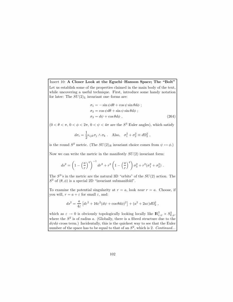
Insert 10: A Closer Look at the Eguchi–Hanson Space; The “Bolt”

Let us establish some of the properties claimed in the main body of the text,while uncovering a useful technique. First, introduce some handy notationfor later: The SU(2)L invariant one–forms are:

σ1 = − sinψdθ + cosψ sin θdφ ;

σ2 = cosψdθ + sinψ sin θdφ ;

σ3 = dψ + cos θdφ , (264)

(0 < θ < π, 0 < φ < 2π, 0 < ψ < 4π are the S3 Euler angles), which satisfy

dσi =1

2ǫijkσj ∧ σk . Also, σ2

1 + σ22 ≡ dΩ2

2 ,

is the round S2 metric. (The SU(2)R invariant choice comes from ψ ↔ φ.)

Now we can write the metric in the manifestly SU(2) invariant form:

ds2 =

(1 −

(ar

)4)−1

dr2 + r2(

1 −(ar

)4)σ2

3 + r2(σ21 + σ2

2) .

The S3’s in the metric are the natural 3D “orbits” of the SU(2) action. TheS2 of (θ, φ) is a special 2D “invariant submanifold”.

To examine the potential singularity at r = a, look near r = a. Choose, ifyou will, r = a+ ε for small ε, and:

ds2 =a

4ε

[dε2 + 16ε2(dψ + cos θdφ)2

]+ (a2 + 2aε)dΩ2

2 ,

which as ε → 0 is obviously topologically looking locally like IR2ε,ψ × S2

θ,φ,

where the S2 is of radius a. (Globally, there is a fibred structure due to thedψdφ cross term.) Incidentally, this is the quickest way to see that the Eulernumber of the space has to be equal to that of an S2, which is 2. Continued...

102

Insert 10: Continued...

Now, the point is that r = a is a true singularity for arbitrary choices ofperiodicity ∆ψ of ψ, since there is a conical deficit angle in the plane. Inother words, we have to ensure that as we get to the origin of the plane, ε = 0,the ψ–circles have circumference 2π, no more or less. Infinitesimmally, wemake those measures with the metric, and so the condition is:

2π = limε→0

(d(2

√aε1/2)∆ψ

dε√

(a/4)ε−1/2

),

which gives ∆Ψ = 2π. So in fact, we must spoil our S3 which was a nice orbitof the SU(2) isometry, by performing an ZZ2 identification on ψ, giving it halfits usual period. In this way, the “bolt” singularity r = a is just a harmlessartefact of coordinates. 65,64 Also, we are left with an SO(3) = SU(2)/ZZ2

isometry of the metric. The space at infinity is S3/ZZ2.

locally. These spaces are classified67 according to their identification at infinity,which can be any discrete subgroup, Γ, 68 of the SU(2) which acts on the S3

at infinity, to give S3/Γ. These subgroups have been classified by McKay,69

and have an A–D–E classification. The metrics on the A–series are knownexplicitly as the Gibbons–Hawking metrics,74 which we shall display later, andEguchi–Hanson is in fact the simplest of this series, corresponding to A1.

75 Weshall later use a D–brane as a probe of string theory on a IR4/ZZ2 orbifold,an example which will show that the string theory correctly recovers all of themetric data (263) of these fixed points, and not just the algebraic data we haveseen here.

For completeness, let us compute one more thing about K3 using thisdescription. The Euler characteristic, in this situation, can be written in twoways 64

χ(K3) =1

32π2

∫

K3

√g(RabcdR

abcd − 4RabRab +R2

)

=1

32π2

∫

K3

√gǫabcdR

abRcd

= − 1

16π2

∫

K3

TrR ∧R = 24 . (265)

Even though no explicit metric for K3 has been written, we can compute χas follows.62,64 If we take a manifold M , divide by some group G, remove

103

some fixed point set F , and add in some set of new manifolds N , the Eulercharacteristic of the new manifold is χ = (χ(M) − χ(F ))/|G| + χ(N). Here,G = R ≡ ZZ2, and the Euler characteristic of the Eguchi–Hanson space is equalto 2, from insert 10 (p.102). That of a point is 1, and of the torus is zero. Wetherefore get χ(K3) = −16/2+32 = 24, which will be of considerable use lateron.

So we have constructed the consistent, supersymmetric string propagationon the K3 manifold, using orbifold techniques. We shall use this manifold toillustrate a number of beautiful properties of D–branes and string theory inthe rest of these lectures. See also Paul Aspinwall’s lectures in this school formore applications of such manifolds to the subject of duality. 73

We should mention in passing that it is possible to construct a whole newclass of string “compactification” vacua by including D–branes in the spectrumin such a way that their contribution to spacetime anomalies, etc, combineswith that of the pure geometry in a way that is crucial to the consistencyof the model. This gives the idea of a “D–manifold” 93,94, which we will notreview here in detail. The analogue of the orbifold method for making these su-persymmetric vacua is the generalised “orientifold” construction already men-tioned. There are constructions of “K3 Orientifolds” which follow the ideaspresented in this section, combined with D–brane orbifold techniques to bedeveloped in later sections. 109,159,160,158,26,161,162 Six dimensional supersym-metric D–manifolds constructed as orientifolds have been constructed.163 Also,there have been important studies of the strong coupling nature of orientifoldvacua, 165 making connections to “F–theory”, 166, some beautiful geometrictechnology for studying type IIB string vacua with variable coupling gs, whichunfortunately we do not have time or space to review here. There are also pureconformal field theory techniques for constructing D–manifolds, which are notpure orbifolds of the type considered here. 164

5.6 T–Duality of Type II Superstrings

T–duality on the closed oriented Type II theories has a somewhat more in-teresting effect than in the bosonic case. 10,6 Consider compactifying a singlecoordinate X9, of radius R. In the R → ∞ limit the momenta are p9

R = p9L,

while in the R → 0 limit p9R = −p9

L. Both theories are SO(9, 1) invariant butunder different SO(9, 1)’s. T–duality, as a right–handed parity transformation(see (128)), reverses the sign of the right–moving X9(z); therefore by super-conformal invariance it does so on ψ9(z). Separate the Lorentz generators into

their left-and right–moving parts Mµν + Mµν . Duality reverses all terms inMµ9, so the µ9 Lorentz generators of the T–dual theory are Mµ9 − Mµ9. In

104

particular this reverses the sign of the helicity s4 and so switches the chiralityon the right–moving side. If one starts in the IIA theory, with opposite chiral-ities, the R → 0 theory has the same chirality on both sides and is the R → ∞limit of the IIB theory, and vice–versa. In short, T–duality, as a one–sidedspacetime parity operation, reverses the relative chiralities of the right– andleft–moving ground states. The same is true if one dualises on any odd numberof dimensions, whilst dualising on an even number returns the original TypeII theory.

Since the IIA and IIB theories have different R–R fields, T9 duality musttransform one set into the other. The action of duality on the spin fields is ofthe form

Sα(z) → Sα(z), Sα(z) → P9Sα(z) (266)

for some matrix P9, the parity transformation (9-reflection) on the spinors. Inorder for this to be consistent with the action ψ9 → −ψ9, P9 must anticom-mute with Γ9 and commute with the remaining Γµ. Thus P9 = Γ9Γ11 (thephase of P9 is determined, up to sign, by hermiticity of the spin field). Nowconsider the effect on the R-R vertex operators (248). The Γ11 just contributesa sign, because the spin fields have definite chirality. Then by the Γ-matrixidentity (249), the effect is to add a 9-index to G if none is present, or toremove one if it is. The effect on the potential C (G = dC) is the same. Takeas an example the Type IIA vector Cµ. The component C9 maps to the IIBscalar C, while the µ 6= 9 components map to Cµ9. The remaining componentsof Cµν come from Cµν9, and so on.

Of course, these relations should be translated into rules for T–dualisingthe spacetime fields in the supergravity actions (251) and (252). The NS–NS sector fields’ transformations are the same as those shown in equations(140),(142), while for the R–R potentials: 60

C(n)µ···ναy = C

(n−1)µ···να − (n− 1)

C(n−1)[µ···ν|yG|α]y

Gyy(267)

C(n)µ···ναβ = C

(n+1)µ···ναβy + nC

(n−1)[µ···ναBβ]y + n(n− 1)

C(n−1)[µ···ν|yB|α|yG|β]y

Gyy

5.7 T–Duality of Type I Superstrings

Just as in the case of the bosonic string, the action of T–duality in the open andunoriented open superstring theory produces D–branes and orientifold planes.Having done it once, (say onX9 with radius R), we get a T9–dual theory on theline interval S1/ZZ2, where ZZ2 acts as the reflection X9 → −X9. The S1 has

105

radius R′ = α′/R). There are 16 D8–branes and their mirror images (comingfrom the 16 D9–branes), together with two orientifold O8–planes located atX9 = 0, πR′. This is called the “Type I′” theory (and sometimes the “Type IA”theory), about which we will have more to say later as well.

Starting with the type IIB theory, we can carry this out n times on ndirections, giving us 16 D(9−n) and their mirror images through 2n O(9−n)–planes arranged on the hypercube of fixed points of T n/ZZ2, where the ZZ2 actsas a reflection in the n directions. If n is odd, we are in type IIA string theory,while we are back in type IIB otherwise.

Let us focus here on a single D–brane, taking a limit in which the otherD–branes and the O–planes are distant and can be ignored. Away from theD–brane, only closed strings propagate. The local physics is that of the TypeII theory, with two gravitinos. This is true even though we began with theunoriented Type I theory which has only a single gravitino. The point is thatthe closed string begins with two gravitinos, one with the spacetime supersym-metry on the right–moving side of the world–sheet and one on the left. Theorientation projection of the Type I theory leaves one linear combination ofthese. But in the T–dual theory, the orientation projection does not constrainthe local state of the string, but relates it to the state of the (distant) imagegravitino. Locally there are two independent gravitinos, with equal chiralitiesif n, (the number of dimensions on which we dualised) is even and opposite ifn is odd.

This is all summarised nicely by saying that while the type I string theorycomes from projecting the type IIB theory by Ω, the T–dual string theoriescome from projecting type II string theory compactified on the torus T n byΩ∏m[Rm(−1)F ], where the product over m is over all the n directions, and

Rm is a reflection in the mth direction. This is indeed a symmetry of thetheory and hence a good symmetry with which to project. So we have thatT–duality takes the orientifold groups into one another:

Ω ↔ 1,Ω∏m[Rm(−1)F ] . (268)

This is a rather trivial example of an orientifold group, since it takes type IIstrings on the torus T n and simply gives a theory which is simply related totype I string theory on T n by n T–dualities. Nevertheless, it is illustrative ofthe general constructions of orientifold backgrounds made by using more com-plicated orientifold groups. This is a useful piece of technology for constructingstring backgrounds with interesting gauge groups, with fewer symmetries, asa starting point for phenomenological applications.

106

5.8 D–Branes as BPS Solitons

While there is type II string theory in the bulk, (i.e., away from the branesand orientifolds), notice that the open string boundary conditions are invariantunder only one supersymmetry. In the original Type I theory, the left–movingworld–sheet current for spacetime supersymmetry jα(z) flows into the bound-ary and the right–moving current jα(z) flows out, so only the total chargeQα + Qα of the left- and right-movers is conserved. Under T–duality thisbecomes

Qα + (∏mPm) Qα , (269)

where the product of reflections Pm runs over all the dualised dimensions, thatis, over all directions orthogonal to the D–brane. Closed strings couple to open,so the general amplitude has only one linearly realized supersymmetry. Thatis, the vacuum without D–branes is invariant under N = 2 supersymmetry,but the state containing the D–brane is invariant under only N = 1: it is aBPS state.76,77

BPS states must carry conserved charges. In the present case there is onlyone set of charges with the correct Lorentz properties, namely the antisym-metric R-R charges. The world volume of a p–brane naturally couples to a(p+ 1)–form potential C(p+1), which has a (p+ 2)-form field strength G(p+2).This identification can also be made from the g−1

s behaviour of the D–branetension: this is the behaviour of an R–R soliton.78,80, as will be developedfurther later.

The IIA theory has Dp–branes for p = 0, 2, 4, 6, and 8. The vertexoperators (248) describe field strengths of all even ranks from 0 to 10. By aΓ-matrix identity the n-form and (10−n)-form field strengths are Hodge dualto one another, so a p–brane and (6 − p)–brane are sources for the same field,but one ‘magnetic’ and one ‘electric.’ The field equation for the 10-form fieldstrength allows no propagating states, but the field can still have a physicallysignificant energy density 76,81,82.

The IIB theory has Dp–branes for p = −1, 1, 3, 5, 7, and 9. The vertexoperators (248) describe field strengths of all odd ranks from 1 to 9, appropriateto couple to all but the 9–brane. The 9–brane does couple to a nontrivialpotential, as we will see below.

A (−1)–brane is a Dirichlet instanton, defined by Dirichlet conditions inthe time direction as well as all spatial directions.83 Of course, it is not clearthat T–duality in the time direction has any meaning, but one can argue forthe presence of (−1)–branes as follows. Given 0–branes in the IIA theory, thereshould be virtual 0–brane world–lines that wind in a purely spatial direction.Such world–lines are required by quantum mechanics, but note that they are

107

essentially instantons, being localised in time. A T–duality in the windingdirection then gives a (−1)–brane. One of the first clues to the relevance ofD–branes,23 was the observation that D–instantons, having action g−1

s , wouldcontribute effects of order e−1/gs as expected from the behaviour of large ordersof string perturbation theory.84

The D–brane, unlike the fundamental string, carries R–R charge. Thisis consistent with the fact that they are BPS states, and so there must be aconserved charge. A more careful argument, involving the R–R vertex opera-tors, can be used to show that they must couple thus, and furthermore thatfundamental strings cannot carry R–R charges.

5.9 The D–Brane Charge and Tension

The bosonic discussion of section 4 will supply us with the worldvolume ac-tion (207) for the bosonic excitations of the D–branes in this supersymmetriccontext. Now that we have seen that Dp–branes are BPS states, and coupleto R–R sector (p+ 1)–form potential, we ought to compute their charges andnew values for the tensions.

Focusing on the R–R sector for now, supplementing the spacetime super-gravity action with the D–brane action we must have at least (recall that thedilaton will not appear here, and also that we cannot write this for p = 3):

S = − 1

2κ20

∫G(p+2)

∗G(p+2) + µp

∫

Mp+1

C(p+1), (270)

where µp is the charge of the Dp–brane under the (p+1)–form C(p+1). Mp+1

is the world–volume of the Dp–brane.Now the same vacuum cylinder diagram as in the bosonic string, as we did

in section 3.10. With the fermionic sectors, our trace must include a sum overthe NS and R sectors, and furthermore must include the GSO projection ontoeven fermion number. Formally, therefore, the amplitude looks like: 76

A =

∫ ∞

0

dt

2tTrNS+R

1 + (−1)F

2e−2πtL0

. (271)

Performing the traces over the open superstring spectrum gives

A = 2Vp+1

∫dt

2t(8π2α′t)−(p+1)/2e−t

Y 2

2πα′

2−1f−81 (q)

−f2(q)8 + f3(q)

8 − f4(q)8,(272)

where again q = e−2πt. The three terms in the braces come from the openstring R sector with 1

2 in the trace, from the NS sector with 12 in the trace, and

108

the NS sector with 12 (−1)F in the trace; the R sector with 1

2 (−1)F gives nonet contribution. In fact, these three terms sum to zero by Jacobi’s “aequatioidentico satis abstrusa”, as they ought to since the open string spectrum issupersymmetric, and we are computing a vacuum diagram.

What does this result mean? Recall that this vacuum diagram also repre-sents the exchange of closed strings between two identical branes. the resultA = 0 is simply a restatement of the fact that D–branes are BPS states: Thenet forces from the NS–NS and R–R exchanges cancel. A = 0 has a usefulstructure, nonetheless, and we can learn more by identifying the separate NS–NS and R–R pieces. This is easy, if we look at the diagram afresh in terms ofclosed string: In the terms with (−1)F , the world–sheet fermions are periodicaround the cylinder thus correspond to R–R exchange. Meanwhile the termswithout (−1)F have anti–periodic fermions and are therefore NS–NS exchange.

Obtaining the t→ 0 behaviour as before (use the limits in insert 8 (p.73))gives

ANS = −AR ∼ 1

2Vp+1

∫dt

t(2πt)−(p+1)/2(t/2πα′)4e−t

Y 2

8π2α′2

= Vp+12π(4π2α′)3−pG9−p(Y2). (273)

Comparing with field theory calculations gives76

2κ20µ

2p = 2κ2τ2

p = 2π(4π2α′)3−p. (274)

Finally, using the explicit expression (254) for κ in terms of string theoryquantities, we get an extremely simple form for the charge:

µp = (2π)−pα′−(p+1)

2 , and τp = g−1s µp . (275)

(For consistency with the discussion in the bosonic case, we shall still use thesymbol Tp to mean τpgs, in situations where we write the action with thedilaton present. It will be understood then that e−Φ contains the requiredfactor of g−1

s .)It is worth updating our bosonic formula (213) for the coupling of the

Yang–Mills theory which appears on the world–volume of Dp–branes with oursuperstring result above, to give:

g2YM,p = τ−1

p (2πα′)−2 = (2π)p−2α′(p−3)/2 , (276)

a formula we will use a lot in what is to follow.Note that our formula for the tension (275) gives for the D1–brane

τ1 =1

2πα′gs, (277)

109

which sets the ratios of the tension of the fundamental string, τF1 ≡ T =

(2πα′)−1 , and the D–string to be simply the string coupling gs. This is a veryelegant normalisation is is extremely natural.

D–branes that are not parallel feel a net force since the cancellation is nolonger exact. In the extreme case, where one of the D–branes is rotated byπ, the coupling to the dilaton and graviton is unchanged but the coupling tothe R–R tensor is reversed in sign. So the two terms in the cylinder amplitudeadd, instead of cancelling, and Jacobi cannot help us. The result is:

A = Vp+1

∫dt

t(2πt)−(p+1)/2e−t(Y

2−2πα′)/8π2α′2

f(t) (278)

where f(t) approaches zero as t→ 0. Differentiating this with respect to Y toextract the force per unit world–volume, we get

F (Y ) = Y

∫dt

t(2πt)−(p+3)/2e−t(Y

2−2πα′)/8π2α′2

f(t) . (279)

The point to notice here is that the force diverges as Y 2 → 2πα′. This issignificant. One would expect a divergence, of course, since the two oppositelycharged objects are on their way to annihilating. 85 The interesting feature itthat the divergence begins when their separation is of order the string length.This is where the physics of light fundamental strings stretching between thetwo branes begins to take over. Notice that the argument of the exponential istU2, where U = Y/(2α′) is the energy of the lightest open string connecting thebranes. A scale like U will appear again, as it is a useful guide to new variablesto D–brane physics at “substringy” distances86,87,88 in the limit where α′ andY go to zero.

Orientifold planes also break half the supersymmetry and are R-R and NS-NS sources. In the original Type I theory the orientation projection keeps onlythe linear combination Qα+ Qα. In the T–dualised theory this becomes Qα+(∏m Pm)Qα just as for the D–branes. The force between an orientifold plane

and a D–brane can be obtained from the Mobius strip as in the bosonic case;again the total is zero and can be separated into NS-NS and R-R exchanges.The result is similar to the bosonic result (197),

µ′p = ∓2p−5µp, τ ′p = ∓2p−5τp . (280)

Since there are 29−p orientifold planes, the total O–plane charge is ∓16µp, andthe total fixed-plane tension is ∓16τp.

A nonzero total tension represents a source for the graviton and dilaton.By the Fischler–Susskind mechanism89, at order gs those background fields

110

become become time dependent as in a consistent way. A non–zero total R–R source is more serious, since this would mean that the field equations areinconsistent (there are uncancelled tadpoles): There is a violation of Gauss’Law, as R–R flux lines have no place to go in the compact space T 9−p. Soour result tells us that on T 9−p, we need exactly 16 D–branes, with the SOprojection, in order to cancel the R–R G(p+2) form charge. This gives theT–dual of SO(32), completing our simple orientifold story.

The spacetime anomalies for G 6= SO(32) are thus accompanied by adivergence90 in the full string theory, as promised, with inconsistent field equa-tions in the R–R sector: As in field theory, the anomaly is related to theultraviolet limit of a (open string) loop graph. But this ultraviolet limit ofthe annulus/cylinder (t → ∞) is in fact the infrared limit of the closed stringtree graph, and the anomaly comes from this infrared divergence. From theworld–sheet point of view, as we have seen in the bosonic case, inconsistencyof the field equations indicates that there is a conformal anomaly that cannotbe cancelled. The prototype of this is the original D = 10 Type I theory.29

The N D9–branes and single O9–plane couple to an R–R 10-form,

(32 ∓N)µ10

2

∫A10, (281)

and the field equation from varying A10 is just G = SO(32).

5.10 Dirac Charge Quantisation

We are of course studying a quantum theory, and so the presence of both mag-netic and electric sources of various potentials in the theory should give somecause for concern. We should check that the values of the charges are consis-tent with the appropriate generalisation of97 the Dirac quantisation condition.The field strengths to which a Dp–brane and D(6 − p)–brane couple are dualto one another, G(p+2) = ∗G(8−p).

We can integrate the field strength ∗G(p+2) on an (8−p)-sphere surround-ing a Dp–brane, and using the action (270), we find a total flux Φ = µp. Wecan write ∗G(p+2) = G(8−p) = dC(7−p) everywhere except on a Dirac “string”(it is really a sheet), at the end of which lives the D(6− p) “monopole”. Then

Φ =1

2κ20

∫

S8−p

∗G(p+2) =1

2κ20

∫

S7−p

C(7−p) . (282)

where we perform the last integral on a small sphere surrounding the Diracstring. A (6 − p)–brane circling the string picks up a phase eiµ6−pΦ. The

111

condition that the string be invisible is

µ6−pΦ =1

2κ20

µ6−pµp = 2πn. (283)

The D–branes’ charges (274) satisfy this with the minimum quantum n = 1.While this argument does not apply directly to the case p = 3, as the

self–dual 5–form field strength has no covariant action, the result follows byT–duality. A topological derivation of the D–brane charge has been given.There are mathematical structures with deep roots, e.g. “K–theory”, whichseem to capture the physics of the R–R charges in string theory, and this is asubject of exciting research. 95,96 The lectures of John Schwarz in this schooldevelop some of the techniques of Sen 16 which are relevant to constructingbranes from the K–theory point of view. 18,19

6 Worldvolume Actions II: Curvature Couplings

6.1 Tilted D–Branes and Branes within Branes

There are additional terms in the action (270) which we just wrote down,involving the D–brane gauge field. Again these can be determined from T–duality. Consider, as an example, a D1–brane in the 1–2 plane. The actionis

µ1

∫dx0 dx1

(C01 + ∂1X

2C02

). (284)

Under a T–duality in the x2–direction this becomes

µ2

∫dx0dx1dx2 (C012 + 2πα′F12C0) . (285)

We have used the T–transformation of the C fields as discussed in section 5.6,and also the recursion relation (183) between D–brane tensions.

This has an interesting interpretation. As we saw before in section 4.1,a Dp–brane tilted at an angle θ is equivalent to a D(p + 1)–brane with aconstant gauge field of strength F = (1/2πα′) tan θ. Now we see that there isadditional structure: the flux of the gauge field couples to the R–R potentialC(p). In other words, the flux acts as a source for a D(p − 1)–brane living inthe worldvolume of the D(p+1)–brane. In fact, given that the flux comes froman integral over the whole world–volume, we cannot localise the smaller braneat a particular place in the world–volume: it is “smeared” or “dissolved” inthe world–volume.

In fact, we shall see when we come to study supersymmetric combina-tions of D–branes that supersymmetry requires the D0–brane to be completely

112

smeared inside the D2–brane. It is clear here how it manages this, by beingsimply T–dual to a tilted D1–brane. We shall see many consequences of thislater.

6.2 Branes Within Branes: Anomalous Gauge Couplings

The T–duality argument of the previous section is easily generalised, with theChern–Simons like result 98,99

µp

∫

Mp+1

[∑pC(p+1)

]∧ Tr e2πα

′F+B , (286)

(We have included non–trivial B on the basis of the argument given at thebeginning of section 4.) So far, the gauge trace has the obvious meaning.We note that there is the possibility that in the full non–Abelian situation,the C can depend on non–commuting transverse fields X i, and so we needsomething more general. We will return to this later. The expansion of theintegrand (286) involves forms of various rank; the notation means that theintegral picks out precisely the terms that are proportional to the volume formof the Dp–brane.

Looking at the first non–trivial term in the expansion of the exponential inthe action we see that there is the term that we studied above correspondingto the dissolution of a D(p− 2)–brane into the sub 2–plane in the Dp–brane’sworld volume formed by the axes X i and Xj, if field strength components Fijare turned on.

At the next order, we have a term which is quadratic in F :

µp(2πα′)2

2

∫C(p−3) ∧ TrF ∧ F =

µp−4

8π2

∫C(p−3) ∧ TrF ∧ F . (287)

We have used the fact that µp−4/µp = (2π√α′)4. Interestingly, we see that

if we excite an instanton configuration on a 4 dimensional sub–space of theDp–brane’s worldvolume, it is equivalent to precisely one unit of D(p − 4)–brane charge! In fact, this term is already recognisable from the study ofconsistency of the type I string theory in ten dimensions from just field theoryconsiderations. There is a modified 3–form field strength, G(3), which is

G(3) = dC(2) −α′

4[ω3Y − ω3L] , (288)

with action

S = − 1

4κ2

∫G(3) ∧∗ G(3) . (289)

113

Since dω3Y = Tr(F ∧ F ) and dω3L = Tr(R ∧ R), this gives, after integratingby parts

α′

8κ2

∫C(6) ∧ (TrF ∧ F − TrR ∧R) . (290)

An evaluation of the coefficient of the quadratic term in F shows that it isprecisely that in (287), for p = 9. Furthermore, the Green–Schwarz anomalycancellation mechanism 90 requires a term

C(2) ∧X8 , (291)

where

X8 =1

(2π)4

(1

48TrF 4 − 1

192TrF 2TrR2

)+

1

128p21(R) − 1

96p2(R) , (292)

the pure gauge part of which can again be found by expanding (286) to quarticorder. The terms involving curvature will be shown to arise in the next section,where the pi, the Pontryagin classes, will be defined very shortly.

Since we see that the gauge couplings are correct, giving the correct resultsknown from ten dimensional string theory, we ought to take seriously theimplications of the terms involving curvature. It is clear that there must becurvature terms in the action for the Dp–branes and Op-planes also.

6.3 Branes Within Branes: Anomalous “Curvature” Couplings

There are indeed curvature terms of the sort which we deduced in the previoussubsection, from knowledge of the anomaly in string theory. Their presencemay be deduced in many other ways, for example using string duality. A morestraightforward way is to generalise the type of anomaly arguments used for theten dimensional type I string supergravity+Yang–Mills case to include not justD9–branes, but all branes, treating them as surfaces upon which anomaloustheories reside. 91,95 A topological argument can be applied to constrain theform of the couplings required on the world–volumes in order to make thebulk+brane theory consistent. We will not review the details of the argumenthere, but merely quote the result: 92,95

µp

∫

Mp+1

∑

i

C(i)

[e2πα

′F+B]√

A(4π2α′R) , (293)

where the “A–roof” or “Dirac” genus has its square root defined as:

√A(R) = 1 − p1(R)

48+ p2

1(R)7

11520− p2(R)

2880+ · · · (294)

114

The pi(R)’s are the ith Pontryagin class. For example,

p1(R) = − 1

8π2TrR ∧R

p2(R) =1

(2π)4

(−1

4TrR4 +

1

8(TrR2)2

), (295)

Expanding, we have

− µp(4π2α′)2

48

∫

Mp+1

C(p−3) ∧ p1(R) . (296)

So we see another way to get a D(p − 4)–brane: wrap the brane on a fourdimensional surface of non–zero p1(R). Indeed, as we saw in equation (265),the K3 surface has p1 = 2χ = 48, and so wrapping a Dp–brane on K3 givesD(p− 4)–brane charge of −1! 92 We will return to this later.

In fact, we can see that this is not the whole story. We can not reproducethe correct coefficient of the curvature terms in (290) from the anomalouscouplings on the D9–branes alone. Happily, there is a nice resolution to thisproblem, 100 which is found with the O9–plane. It is present since the type Istring theory is an orientifold of the Type IIB theory. An O9–brane does nothave open strings ending on it, as we have seen, and therefore there are nogauge fields on their world–volume. This fits with the fact that we alreadyhave the correct gauge couplings of type I. As they are objects with finitetension, however, they are natural candidates to have curvature couplings. Toget the coupling in (290) right, it can be seen that there must be a coupling(p = 9):

(π2α′)2µp48π2

∫C(p−3) ∧ TrR ∧R (297)

on its worldvolume, (µp = −25−pµp), and we have written the general expres-sion at this order for all negative Op–planes. This (for p = 9) combined withthe contribution from the sixteen D9–branes, gives the correct total curvaturecoupling.

In general, the couplings for this class of Op–planes may be deduced fromanomaly–inflow type arguments, 101 as was the case for the Dp–branes, and ageneral formula written in terms of a index, just like the D–brane case. Theanswer is: 103

µp

∫

Mp+1

∑

i

C(i)

√L(π2α′R) , (298)

115

where the “Hirzebruch” polynomial, L, has its square root defined as:√L(R) = 1 +

p1(R)

6− p2

1(R)1

90+ p2(R)

7

90+ · · · (299)

In fact, the fourth order terms also give us the correct couplings to completethe C(2) ∧X8 needed for consistency. There are more general types of O–planein string theory than the type we have considered here, and for which curvaturecouplings have been derived. 102,104,105

6.4 Further Non–Abelian Extensions

One can use T–duality to go a bit further and deduce the non–Abelian formof the action, being mindful of the sort of complications mentioned at thebeginning of section (4.4). In the absence of curvature terms i it turns out tobe: 44,45

µp

∫

p−brane

Tr([e2πα

′iΦiΦ

∑pC(p+1)

]e2πα

′F+B). (300)

Here, we ascribe the same meaning to the gauge trace as we did previously(see section (4.4)). The meaning of iX is as the “interior product” in thedirection given by the vector Φi, which produces a form of one degree fewer inrank. For example, on a two form C(2)(Φ) = (1/2)Cij(Φ)dX idXj, we have

iΦC(2) = ΦiCij(Φ)dXj ; iΦiΦC(2)(Φ) = ΦjΦiCij(Φ) =1

2[Φi,Φj ]Cij(Φ) ,

(301)where we see that the result of acting twice is non–vanishing when we allowfor the non–abelian case, with C having a nontrivial dependence on Φ. Weshall see this action work for us to produce interesting physics later.

6.5 Even More Curvature Couplings

We deduced curvature couplings to the R–R potentials a few subsections ago.In particular, such couplings induce the charge of lower p branes by wrappinglarger branes on topologically non–trivial surfaces.

In fact, as we saw before, if we wrap a Dp–brane on K3, there is inducedprecisely −1 units of charge of a D(p− 4)–brane. This means that the chargeof the effective (p− 4)–dimensional object is

µ = µpVK3 − µp−4 , (302)iAn important issue is the nature of the coupling of curvature and R–R potentials in suchnon–Abelian situations. Given the enhancon phenomenon discussed later on, it is clear thatthere are such effective couplings.

116

where VK3 is the volume of the K3. However, we can go further and notice thatsince this is a BPS object of the six dimensional N = 2 string theory obtainedby compactifying on K3, we should expect that it has a tension which is

τ = τpVK3 − τp−4 = g−1s µ . (303)

If this is indeed so, then there must be a means by which the curvature of K3induces a shift in the tension in the world–volume action. Since the part of theaction which refers to the tension is the Dirac–Born–Infeld action, we deducethat there must be a set of curvature couplings for that part of the action aswell.100 Some of them are given by the following: 100,106

S = −τp∫dp+1ξ e−Φdet1/2(Gab + Fab)

(1 − 1

768π2×

(RabcdRabcd −RαβabR

αβab + 2RαβRαβ − 2RabRab)

+O(α′4)

),

(304)

where Rabcd = (4π2α′)Rabcd, etc., and a, b, c, d are the usual tangent spaceindices running along the brane’s world volume, while α, β are normal indices,running transverse to the world–volume.

Some explanation is needed. Recall: the embedding of the brane into D–dimensional spacetime is achieved with the functionsXµ(ξa), (a = 0, . . . , p;µ =0, . . . , D− 1) and the pullback of a spacetime field Fµ is performed by soakingup spacetime indices µ with the local “tangent frame” vectors ∂aX

µ, to giveFa = Fµ∂aX

µ. There is another frame, the “normal frame”, with basis vectorsζµα , (α = p+ 1, . . . , D − 1). Orthonormality gives ζµαζ

νβGµν = δαβ and also we

have ζµα∂aXνGµν = 0.

We can pull back the spacetime Riemann tensor Rµνκλ in a number of

ways, using these different frames, as can be seen in the action. R with twoindices are objects which were constructed by contraction of the pulled–backfields. They are not the pull back of the bulk Ricci tensor, which vanishes atthis order of string perturbation theory anyway.

In fact, for the case of K3, it is Ricci flat and everything with normalspace indices vanishes and so we get only RabcdR

abcd appearing, which alonecomputes the result (265) for us, and so after integrating over K3, the actionbecomes:

S = −∫dp−3ξ e−Φ [τpVK3 − τp−4] det1/2(Gab + Fab) , (305)

117

where again we have used the recursion relation between the D–brane tensions.So we see that we have correctly reproduced the shift in the tension that weexpected on general grounds for the effective D(p− 4)–brane. We will use thisaction later.

7 The Dp–Dp′ System

Simple T–duality gives parallel D–branes all with the same dimension but wecan consider more general configurations. In this section we consider two D–branes, Dp and Dp′, each parallel to the coordinate axes. (We can of coursehave D–branes at angles, 107 but we will not consider this here.) An openstring can have both ends on the same D–brane or one on each. The p− p andp′ − p′ spectra are the same as before, but the p − p′ strings are new. Sincewe are taking the D–branes to be parallel to the coordinate axes, there arefour possible sets of boundary conditions for each spatial coordinate X i of theopen string, namely NN (Neumann at both ends), DD, ND, and DN. Whatreally will matter is the number ν of ND plus DN coordinates. A T–dualitycan switch NN and DD, or ND and DN, but ν is invariant. Of course ν is evenbecause we only have p even or p odd in a given theory.

The respective mode expansions are

NN: Xµ(z, z) = xµ − iα′pµ ln(zz) + i

√α′

2

∑

m 6=0

αµmm

(z−m + z−m),

DN,ND: Xµ(z, z) = i

√α′

2

∑

r∈ZZ+1/2

αµrr

(z−r ± z−r), (306)

DD: Xµ(z, z) = −i δXµ

2πln(z/z) + i

√α′

2

∑

m 6=0

αµmm

(z−m − z−m) .

In particular, the DN and ND coordinates have half–integer moding. Thefermions have the same moding in the Ramond sector (by definition) andopposite in the Neveu–Schwarz sector. The string zero point energy is 0 in theR sector as always, and using (79) we get:

(8 − ν)

(− 1

24− 1

48

)+ ν

(1

48+

1

24

)= −1

2+ν

8(307)

in the NS sector.The oscillators can raise the level in half–integer units, so only for ν a

multiple of 4 is degeneracy between the R and NS sectors possible. Indeed,

118

it is in this case that the Dp–Dp′ system is supersymmetric. We can see thisdirectly. As discussed in sections 5.6 and 5.8, a D–brane leaves unbroken thesupersymmetries

Qα + PQα , (308)

where P acts as a reflection in the direction transverse to the D–brane. Witha second D–brane, the only unbroken supersymmetries will be those that arealso of the form

Qα + P ′Qα = Qα + P (P−1P ′)Qα . (309)

with P ′ the reflection transverse to the second D–brane. Then the unbrokensupersymmetries correspond to the +1 eigenvalues of P−1P ′. In DD and NNdirections this is trivial, while in DN and ND directions it is a net paritytransformation. Since the number ν of such dimensions is even, we can pairthem as we did in section 5.1, and write P−1P ′ as a product of rotations by π,

eiπ(J1+...+Jν/2) . (310)

In a spinor representation, each eiπJ has eigenvalues ±i, so there will be un-broken supersymmetry only if ν is a multiple of 4 as found above. j

For example, Type I theory, besides the D9–branes, will have D1–branesand D5–branes. This is consistent with the fact that the only R-R fieldstrengths are the three-form and its Hodge–dual seven–form. The D5–braneis required to have two Chan–Paton degrees of freedom (which can be thoughtof as images under Ω) and so an SU(2) gauge group.108,109

When ν = 0, P−1P ′ = 1 identically and there is a full ten-dimensionalspinor of supersymmetries. This is the same as for the original Type I theory,to which it is T–dual. In D = 4 units, this is N = 4, or sixteen supercharges.For ν = 4 or ν = 8 there is D = 4 N = 2 supersymmetry.

Let us now study the spectrum for ν = 4, saving ν = 8 for later. Sometimesit is useful to draw a quick table showing where the branes are located. Here isone for the (9,5) system, where the D5–brane is pointlike in the x6, x7, x8, x9

directions and the D9–brane is (of course) extended everywhere:

x0 x1 x2 x3 x4 x5 x6 x7 x8 x9

D9 − − − − − − − − − −D5 − − − − − − • • • •

A dash under xi means that the brane is extended in that direction, while adot means that it is pointlike there.

jWe will see that there are supersymmetric bound states when ν = 2.

119

Continuing with our analysis, we see that the NS zero–point energy iszero. There are four periodic world–sheet fermions ψi, namely those in theND directions. The four zero modes generate 24/2 or four ground states, ofwhich two survive the GSO projection. In the R sector the zero–point energy isalso zero; there are four periodic transverse ψ, from the NN and DD directionsnot counting the directions µ = 0, 1. Again these generate four ground statesof which two survive the GSO projection. The full content of the p–p′ systemis then is half of an N = 2 hypermultiplet. The other half comes from thep′–p states, obtained from the orientation reversed strings: these are distinctbecause for ν 6= 0 the ends are always on different D–branes.

Let us write the action for the bosonic p − p′ fields χA, starting with(p, p′) = (9, 5). Here A is a doublet index under the SU(2)R of the N = 2algebra. The field χA has charges (+1,−1) under the U(1)×U(1) gauge theo-ries on the branes, since one end leaves, and the other arrives. The minimallycoupled action is then

∫d6ξ

(5∑

a=0

|(∂a + iAa − iA′a)χ|

2+

(1

4g2YM,p

+1

4g2YM,p′

) 3∑

I=1

(χ†τIχ)2

),

(311)with Aa and A′

a the brane gauge fields, gYM,p and gYM,p′ the effective Yang–Mills couplings (276), and τI the Pauli matrices. The second term is from theN = 2 D–terms for the two gauge fields. It can also be written as a commutatorTr [φi, φj ]2 for appropriately chosen fields φi, showing that its form is controlledby the dimensional reduction of an F 2 pure Yang–Mills term. See section 9.1for more on this.

The integral is over the 5–brane world-volume, which lies in the 9–braneworld-volume. Under T–dualities in any of the ND directions, one obtains(p, p′) = (8, 6), (7, 7), (6, 8), or (5, 9), but the intersection of the branes re-mains (5 + 1)-dimensional and the p–p′ strings live on the intersection withaction (311). In the present case the D-term is nonvanishing only for χA = 0,though more generally (say when there are several coincident p and p′–branes),there will be additional massless charged fields and flat directions arise.

Under T–dualities in r NN directions, one obtains (p, p′) = (9 − r, 5 − r).The action becomes

∫d6−rξ

(5−r∑

a=0

|(∂a + iAa − iA′a)χ|

2+

χ†χ

(2πα′)2

5∑

a=6−r

(Xa −X ′a)

2

+

(1

4g2YM,p

+1

4g2YMp′

) 3∑

i=1

(χ†τIχ)2

). (312)

120

The second term, proportional to the separation of the branes, is from thetension of the stretched string.

7.1 The BPS Bound

The ten dimensional N = 2 supersymmetry algebra (in a Majorana basis) is

Qα, Qβ = 2(Γ0Γµ)αβ(Pµ +QNSµ /2πα′)

Qα, Qβ = 2(Γ0Γµ)αβ(Pµ −QNSµ /2πα′)

Qα, Qβ = 2∑

p

τpp!

(Γ0Γm1 . . .Γmp)αβQRm1...mp

. (313)

Here QNS is the charge to which the NS–NS two–form couples, it is essentiallythe winding of a fundamental string stretched along M1:

QNSµ ≡ QNS

v1

∫

M1

dXµ , with QNS =1

VolS7

∫

S7

e−2Φ ∗H(3) (314)

and the charge QNS is normalised to one per unit spatial world–volume, v1 =L, the length of the string. It is obtained by integrating over the S7 whichsurrounds the string. The QR are the R–R charges, defined as a generalisationof winding on the space Mp:

QRµ1...µp

≡ QRp

vp

∫

Mp

dXµ1 ∧ · · ·dXµp , with QRp =

1

VolS8−p

∫

S8−p

∗G(p+2) .

(315)

The sum in (313) runs over all orderings of indices, and we divide by p! Ofcourse, p is even for IIA or odd for IIB. The R–R charges appear in the productof the right- and left–moving supersymmetries, since the corresponding vertexoperators are a product of spin fields, while the NS-NS charges appear inright–right and left–left combinations of supercharges.

As an example of how this all works, consider an object of length L, withthe charges of p fundamental strings (“F–strings”, for short) and q D1–branes(“D–strings) in the IIB theory, at rest and aligned along the direction X1. Theanticommutator implies

1

2

[QαQα

],[Qβ Qβ

]=

[1 00 1

]Mδαβ +

[p q/gs

q/gs −p

]L(Γ0Γ1)αβ

2πα′.

(316)

121

The eigenvalues of Γ0Γ1 are ±1 so those of the right–hand side are M ±L(p2 +q2/g2)1/2/2πα′. The left side is a positive matrix, and so we get the “BPSbound” on the tension110

M

L≥√p2 + q2/g2

s

2πα′≡ τp,q . (317)

Quite pleasingly, this is saturated by the fundamental string, (p, q) = (1, 0),and by the D–string, (p, q) = (0, 1).

It is not too hard to extend this to a system with the quantum numbersof Dirichlet p and p′ branes. The result for ν a multiple of 4 is

M ≥ τpvp + τp′vp′ (318)

and for ν even but not a multiple of 4 it is k

M ≥√τ2p v

2p + τ2

p′v2p′ . (319)

The branes are wrapped on tori of volumes vp and v′p in order to make themasses finite.

The results (318) and (319) are consistent with the earlier results on super-symmetry breaking. For ν a multiple of 4, a separated p–brane and p′–branedo indeed saturate the bound (318). For ν not a multiple of four, they do notsaturate the bound (319) and cannot be supersymmetric.

7.2 FD Bound States

Consider a parallel D–string and F–string lying along X1. The total tension

τD1 + τF1 =g−1s + 1

2πα′(320)

exceeds the BPS bound (317) and so this configuration is not supersymmetric.However, it can lower its energy24 as shown in figure 23. The F–string breaks,its endpoints attached to the D–string. The endpoints can then move off toinfinity, leaving only the D–string behind. Of course, the D–string must nowcarry the charge of the F-string as well. This comes about because the F–stringendpoints are charged under the D–string gauge field, so a flux runs betweenthem; this flux remains at the end. Thus the final D–string carries both theNS–NS and R–R two–form charges. The flux is of order gs, its energy density

kThe difference between the two cases comes from the relative sign of ΓM (ΓM′

)T and

ΓM′

(ΓM )T .

122

(a) (c)(b)

Figure 23: (a) A parallel D–string and F–string, which is not supersymmetric. (b) TheF–string breaks, its ends attaching to the D-string, resulting in (c) the final supersymmetricstate, a D–string with flux.

is of order gs, and so the final tension is (g−1s +O(gs))/2πα

′. This is below thetension of the separated strings and of the same form as the BPS bound (317)for a (1, 1) string. A more detailed calculation shows that the final tensionsaturates the bound, 98 so the state is supersymmetric. In effect, the F–stringhas dissolved into the D–string, leaving flux behind.

We can see quite readily that this is a supersymmetric situation usingT–duality. We can choose a gauge in which the electric flux is F01 = A1.T–dualizing along the x1 direction, we ought to get a D0–brane, which we do,except that it is moving with constant velocity, since we get X1 = 2πα′A1.This clearly has the same supersymmetry as a stationary D0–brane, havingbeen simply boosted.

To calculate the number of BPS states we should put the strings in abox of length L to make the spectrum discrete. For the (1, 0) F-string, theusual quantisation of the ground state gives eight bosonic and eight fermionicstates moving in each direction for 162 = 256 in all. This is the ultrashortrepresentation of supersymmetry: half the 32 generators annihilate the BPSstate and the other half generate 28 = 256 states. The same is true of the(0, 1) D-string and the (1, 1) bound state just found, as will be clear from thelater duality discussion of the D–string.

It is worth noting that the (1, 0) F–string leaves unbroken half the su-persymmetry and the (0, 1) D–string leaves unbroken a different half of thesupersymmetry. The (1, 1) bound state leaves unbroken not the intersection of

123

the two (which is empty), but yet a different half. The unbroken symmetriesare linear combinations of the unbroken and broken supersymmetries of theD–string.

All the above extends immediately to p F–strings and one D–string, form-ing a supersymmetric (p, 1) bound state. The more general case of p F-stringsand q D–strings is more complicated. The gauge dynamics are now non–Abelian, the interactions are strong in the infrared, and no explicit solutionis known. When p and q have a common factor, the BPS bound makes anybound state only neutrally stable against falling apart into subsystems. Toavoid this complication let p and q be relatively prime, so any supersymmetricstate is discretely below the continuum of separated states. This allows theHamiltonian to be deformed to a simpler supersymmetric Hamiltonian whosesupersymmetric states can be determined explicitly, and again there is one ul-trashort representation, 256 states. The details, which are quite intricate, areleft to the reader to consult in the literature 24,1.

7.3 The Three–String Junction

Let us consider further the BPS saturated formula derived and studied in thetwo previous subsections, and write it as follows:

τp,q =√

(pτ1,0)2 + (qτ0,1)2 . (321)

An obvious solution to this is

τp,q sinα = qτ0,1 , τp,q cosα = pτ1,0 . (322)

with tanα = q/(pgs). Recall that these are tensions of strings, and thereforewe can interpret the equations (322) as balance conditions for the componentsof forces! In fact, it is the required balance for three strings, 113,111 and wedraw the case of p = q = 1 in figure 24.

Is this at all consistent with what we already know? The answer is yes.An F–string is allowed to end on a D–string by definition, and a (1,1) stringis produced, due to flux conservation, as we discussed above. The issue here isjust how we see that there is bending. The first thing to notice is that the angleα goes to π/2 in the limit of zero string coupling, and so the D–string appearsin that case to run straight. This had better be true, since it is then clear thatwe simply were allowed to ignore the bending in our previous weakly coupledstring analysis. (This study of the bending of branes beyond zero coupling hasimportant consequences for the study of one–loop gauge theory data. 114 Weshall study some of this later on.)

124

α

x

x

1

2

(1,0)

(1,1)

(0,1)

(a)

x

x

1

2

(1,0)

(1,1)

(b)

(0,1)

α

β

Figure 24: (a) When an F–string ends on a D–string it causes it to bend at an angle set bythe string coupling. On the other side of the junction is a (1,1) string. This is in fact a BPSstate. (b) Switching on some amount of the R–R scalar can vary the other angle, as shown.

Parenthetically, it is nice to see that in the limit of infinite string coupling,α goes to 0. The diagram is better interpreted as a D–string ending on an F–string with no resulting bending. This fits nicely with the fact that the D– andF–strings exchange roles under the strong/weak coupling duality (“S–duality”)of the type IIB string theory.

When we wrote the linearized BIon equations in section 4.6, we ignoredthe 1+1 dimensional case. Let us now include that part of the story here asa 1+1 dimensional gauge theory discussion. There is a flux F01 on the world–volume, and the end of the F–string is an electric source. Given that there isonly one spatial dimension, the F–string creates a discontinuity on the flux,such that e.g: 115,50

F01 =

gs , x1 > 00 , x1 < 0

, (323)

so we can choose a gauge such that

A0 =

gsx

1 , x1 > 00 , x1 < 0

. (324)

Just as in section 4.6, this is BPS is one of the eight scalars Φm is also switchedon so that

Φ2(x1) = A0 . (325)

125

How do we interpret this? Since (2πα′)Φ2 represents the x2 position of theD–string, we see that for x1 < 0 the D–string is lying along the x1 axis, whilefor x1 > 0, it lies on a line forming an angle tan−1(1/gs) with the x1, axis.

Recall the T1–dual picture we mentioned in the previous section, where wesaw that the flux on the D–string (making the (1,1) string) is equivalent to aD0–brane moving with velocity (2πα′)F01. Now we see that the D0–brane losesits velocity at x1 = 0. This is fine, since the apparent impulse is accountedfor by the momentum carried by the F–string in the T–dual picture. (One hasto tilt the diagram in order to T–dualize along the (1,1) string in order to seethat there is F–string momentum.)

Since as we have seen many times that the presence of flux on the world–volume of a Dp–brane is equivalent to having a dissolved D(p− 2)–brane, i.e.,non–zero C(p−1) source, we can modify the flux on the x1 < 0 part of thestring this way by turning on the R–R scalar C0. This means that Φ2(x1) willbe linear there too, and so the angle β between the D– and F–strings can bevaried too (see figure 24(b)). It is interesting to derive the balance conditionsfrom this, and then convert it into a modified tension formula, but we will notdo that here. 115

It is not hard to imagine that given the presence we have already deducedof a general (p, q) string in the theory that there are three–string junctions tobe made out of any three strings such that the (p, q)–charges add up correctly,giving a condition on the angles at which they can meet. This is harder todo in the full non–Abelian gauge theories on their world–volumes, but in facta complete formula can be derived using the underlying SL(2,ZZ) symmetryof the type IIB string theory. We will have more to say about this symmetrylater.

General three–string junctions have been shown to be important in a num-ber of applications, and there is a large literature on the subject which we areunfortunately not able to review here.

7.4 0–p Bound States

Bound states of p–branes and p′–branes have many applications. Some of themwill appear in our later lectures, and so it is worth listing some of the resultshere. Here we focus on p′ = 0, since we can always reach it from a general(p, p′) using T–duality.

• 0–0 bound states:

The BPS bound for the quantum numbers of n 0–branes is nτ0, so anybound state will be at the edge of the continuum. What we would like to

126

know is if there is actually a true bound state wave function, i.e., a wavefunc-tion which is normalisable. To make the bound state counting well defined,compactify one direction and give the system momentum m/R with m and nrelatively prime. 116 The bound state now lies discretely below the continuum,because the momentum cannot be shared evenly among unbound subsystems.

This bound state problem is T–dual to the one just considered. Taking theT–dual, the n D0–branes become D1–branes, while the momentum becomeswinding number, corresponding to m F-strings. There is therefore one ultra-short multiplet of supersymmetric states whenm and n are relatively prime.116

This bound state should still be present back in infinite volume, since one cantake R to be large compared to the size of the bound state. There is a dangerthat the size of the wavefunction we have just implicitly found might simplygrow with R such that as R → ∞ it becomes non–normalisable again. Morecareful analysis is needed to show this. It is sufficient to say here that the boundstates for arbitrary numbers of D0–branes are needed for the consistency ofstring duality, so this is an important problem. Some strong arguments havebeen presented in the literature, (n = 2 is proven) but the general case is notyet proven. We give an embarrasingly incomplete list of papers in this topicin references. 117

• 0–2 bound states:

Now the BPS bound (319) puts any bound state discretely below thecontinuum. One can see a hint of a bound state forming by noticing that fora coincident D0–brane and D2–brane the NS 0–2 string has a negative zero–point energy (307) and so a tachyon (which survives the GSO projection),indicating instability towards something. In fact the bound state (one shortrepresentation) is easily described: the D0–brane dissolves in the D2–brane,leaving flux, as we have seen numerous times. The brane R–R action (286)contains the coupling C(1)F , so with the flux the D2–brane also carries theD0–brane charge. 118 There is also one short multiplet for n D0–branes. Thissame bound state is always present when ν = 2.

• 0–4 bound states:

The BPS bound (318) makes any bound state marginally stable, so theproblem is made well–defined as in the 0–0 case by compactifying and addingmomentum.119 The interactions in the action (312) are relevant in the infraredso this is again a hard problem, but as before it can be deformed into a solv-able supersymmetric system. Again there is one multiplet of bound states. 119

127

Now, though, the bound state is invariant only under 14 of the original super-

symmetry, the intersection of the supersymmetries of the D0–brane and of theD4–brane. The bound states then lie in a short (but not ultrashort) multipletof 212 states.

For 2 D0–branes and one D4–brane, one gets the correct count as fol-lows. 120 Think of the case that the volume of the D4–brane is large. The 16supersymmetries broken by the D4–brane generate 256 states that are delocal-ized on the D4–brane. The 8 supersymmetries unbroken by the D4–brane andbroken by the D0–brane generate 16 states (half bosonic and half fermionic),localized on the D0–brane. The total number is the product 212. Now countthe number of ways two D0–branes can be put into their 16 states on the D4–brane: there are 8 states with both D0–branes in the same (bosonic) state and1216 · 15 states with the D–branes in different states, for a total of 8 · 16 states.But in addition, the two–branes can bind, and there are again 16 states wherethe bound state binds to the D4–brane. The total, tensoring again with theD4–brane ground states, is 9 · 16 · 256.

For n D0–branes and one D4–brane, the degeneracy Dn is given by thegenerating functional 120

∞∑

n=0

qnDn = 256

∞∏

k=1

(1 + qk

1 − qk

)8

, (326)

where the term k in the product comes from bound states of k D0–branes thenbound to the D4–brane. A recent paper discussing the D0–D4 bound state,with more references, can be found in the references. 121

• 0–6 bound states:

The relevant bound is (319) and again any bound state would be below thecontinuum. The NS zero-point energy for 0–6 strings is positive, so there is nosign of decay. One can give D0–brane charge to the D6–brane by turning onflux, but there is no way to do this and saturate the BPS bound. So it appearsthat there are no supersymmetric bound states. Incidentally, and unlike the0–2 case, the 0–6 interaction is repulsive, both at short distance and at long. 1

• 0–8 bound states:

The case of the D8–brane is special, since it is rather big. It is a domainwall, since there is only one spatial dimension transverse to it. In fact, theD8–brane on its own is not really a consistent object. Trying to put it into

128

type IIA runs into trouble, since the string coupling blows up a finite distancefrom it on either side because of the nature of its coupling to the dilaton. Tostop this happening, one has to introduce a pair of O8–planes, one on eachside, since they (for SO groups) have negative charge (−8 times that of theD8–brane) and can soak up the dilaton. We therefore should have 16 D8–branes for consistency, and so we end up in the type I′ theory, the T–dual ofType I. The bound state problem is now quite different, and certain detailsof it pertain to the strong coupling limit of certain string theories, and their“matrix” 129 formulation. 122,123 We shall revisit this in section 8.5.

8 D–Branes, Strong Coupling, and String Duality

One of the most striking results of the middle ’90’s was the realization that all ofthe string theories are in fact dual to one another at strong coupling.125,126,127 l

This also brought eleven dimensional supergravity in the picture and startedthe search for M–theory, the dynamical theory within which all of those theorieswould fit as various effective descriptions of perturbative limits.

All of this is referred to as the “Second Superstring Revolution”. Everyrevolution is supposed to have a hero or heroes. We shall consider branes tobe cast in that particular role, since they (and D–branes especially) suppliedthe truly damning evidence of the strong coupling fate of the various strigntheories.

We shall discuss aspects of this in the present section. We simply study theproperties of various D–branes in the various string theories, and then trust tothat fact that as they are BPS states, many of these properties will survive atstrong coupling.

8.1 D1–Brane Collective Dynamics

Let us first study the D1–brane. This will be appropriate to the study oftype IIB and the type I string by Ω–projection. Its collective dynamics as aBPS soliton moving in flat ten dimensions is captured by the 1+1 dimensionalworld–volume theory, with 16 or 8 supercharges, depending upon the theorywe are in. (See figure 25(a).)

It is worth first setting up a notation and examining the global symmetries.Let us put the D1–brane to lie along the x1 direction, as we will do many timesin what is to come. This arrangement of branes breaks the Lorentz group upas follows:

lThere are excellent reviews in the literature, some of which are listed in the bibliogra-phy. 128,111,112

129

SO(1, 9) ⊃ SO(1, 1)01 × SO(8)2−9 , (327)

Accordingly, the supercharges decompose under (327) as

16 = 8+ + 8− (328)

where ± subscripts denote a chirality with respect to SO(1, 1).For the 1–1 strings, there are 8 Dirichlet–Dirichlet (DD) directions, the

Neveu–Schwarz (NS) sector has zero point energy −1/2. The massless excita-tions form vectors and scalars in the 1+1 dimensional model. For the vectors,the Neumann–Neumann (NN) directions give a gauge field Aµ. Now, the gaugefield has no local dynamics, so the only contentful bosonic excitations are thetransverse fluctuations. These come from the 8 Dirichlet–Dirichlet (DD) di-rections xm, m = 2, · · · , 9, and are

φm(x0, x1) : λφψm− 1

2|0 > . (329)

The fermionic states ξ from the Ramond (R) sector (with zero point en-ergy 0, as always) are built on the vacua formed by the zero modes ψi0, i=0, . . . , 9.This gives the initial 16. The GSO projection acts on the vacuum in this sectoras:

(−1)F = eiπ(S0+S1+S2+S3+S4) . (330)

A left or right–moving state obeys Γ0Γ1ξ± = ±ξ±, and so the projection onto(−1)F ξ=ξ says that left and right moving states are odd and (respectively)even under Γ2 . . .Γ9, which is to say that they are either in the 8s or the 8c.So we see that the GSO projection simply correlates world sheet chirality withspacetime chirality: ξ− is in the 8c of SO(8) and ξ+ is in the 8s.

8.2 Type IIB/Type IIB Duality

So we have seen that for a D1–brane in type IIB string theory, the right–movingspinors are in the 8s of SO(8), and the left-moving spinors in the 8c. Theseare the same as the fluctuations of a fundamental IIB string, in static gauge.24

There, the supersymmetries Qα and Qα have the same chirality. Half of eachspinor annihilates the F-string and the other half generates fluctuations. Sincethe supersymmetries have the same SO(9, 1) chirality, the SO(8) chirality iscorrelated with the direction of motion.

So far we have been using the string metric. We can switch to the Einstein

metric, g(E)µν = e−Φ/2g

(S)µν , since in this case gravitational action has no depen-

dence on the dilaton, and so it is an invariant under duality. The tensions in

130

this frame are:

F–string: g1/2s /2πα′

D–string: g−1/2s /2πα′ . (331)

Since these are BPS states, we are able to trust these formulae at arbitraryvalues of gs.

Let us see what interpretation we can make of these formulae: At weakcoupling the D–string is heavy and the F–string tension is the lightest scalein the theory. At strong coupling, however, the D–string is the lightest objectin the theory, (A dimensional argument shows that the lowest–dimensionalbranes have the lowest scale. 124) and it is natural to believe that the theorycan be reinterpreted as a theory of weakly coupled D–strings, with g′s = g−1

s .One cannot prove this without a non–perturbative definition of the theory,but quantising the light D–string implies a large number of the states thatwould be found in the dual theory, and self–duality of the IIB theory seems byfar the simplest interpretation—given that physics below the Planck energy isdescribed by some specific string theory, it seems likely that there is a uniqueextension to higher energies. This agrees with the duality deduced from thelow energy action and other considerations. 125,127,135 In particular, the NS–NS and R–R two-form potentials, to which the D– and F–strings respectivelycouple, are interchanged by this duality.

This duality also explains our remark about the strong and weak couplinglimits of the three string junction depicted in figure 24. The roles of the D–and F–strings are swapped in the gs → 0,∞ limits, which fits with the twolimiting values α→ π/2, 0.

The full duality group of the D = 10 Type IIB theory is expected to beSL(2,ZZ).125,127 This relates the fundamental string not only to the R–R stringbut to a whole set of strings with the quantum numbers of p F–strings and qD–strings for p and q relatively prime.110 The bound states found in section 7.2are just what is required for SL(2,ZZ) duality. 24 As the coupling and the R–Rscalar are varied, each of these strings becomes light at the appropriate pointin moduli space.

8.3 Type I/Heterotic

Let us now consider the D1–brane in the Type I theory. We must modify ourprevious analysis in two ways. First, we must project onto Ω–even states.

As in section 2.6, the U(1) gauge field A is in fact projected out, since ∂tis odd under Ω. The normal derivative ∂n, is even under Ω, and hence the Φm

131

survive. Turning to the fermions, we see that Ω acts as eiπ(S1+S2+S3+S4) andso the left–moving 8c is projected out and the right-moving 8s survives.

Recall that D9–branes must be introduced after doing the Ω projection ofthe type IIB string theory. These are the SO(32) Chan–Paton factors. Thismeans that we must also include the massless fluctuations due to strings withone end on the D1-brane and the other on a D9–brane. (See figure 25(b)) Thezero point energy in the NS sector for these states is 1/2, and so there is way tomake a massless state. The R sector has zero point energy zero, as usual, andthe ground states come from excitations in the x0, x1 direction, since it is in theNN sector that the modes are integer. The GSO projection (−)F = Γ0Γ1 will

(b)(a)

Figure 25: D1–branes (a) in Type IIB theory its fluctuations are described by 1–1 strings.(b) in Type I string theory, there are additional contributions from 1–9 strings.

project out one of these, λ−, while the right moving one will remain. The Ωprojection simply relates 1–9 strings to 9–1 strings, and so places no constrainton them. Finally, we should note that the 1–9 strings, as they have one endon a D9–brane, transform as vectors of SO(32).

Now, by the argument that we saw in the case of the type IIB string, weshould deduce that this string becomes a light fundamental string in some dualstring theory at strong coupling. In these notes we have not seen such a stringbefore. It has (0, 8 world sheet supersymmetry, and a left moving family of 32fermions transforming as the 32 of SO(32).

Happily, there is precisely one such string theory in ten dimensions withthis property. It is a closed string theory called the SO(32) “heterotic” string.17

There is in fact another ten dimensional heterotic string, with gauge groupE8×E8. It has a storng coupling limit we will examine shortly. Upon compactifyingon a circle, the two heterotic string theories are perturbatively related by T–duality. 143,144

We have obtained the SO(32) string here with the spacetime supersymme-try realized in Green–Schwarz form and with a left–moving “current algebra”in fermionic form 133, which realises a spacetime SO(32) gauge symmetry. Infact, recall that we had already deduced that such a string theory might ex-

132

ist, by looking at the supergravity sector in section 5.4. This is just howtype I/heterotic duality was deduced first 127, 135 and then D–brane construc-tions were used to test it more sharply 133.

Actually, heterotic string experts know that the fermionic SO(32) currentalgebra requires a GSO projection. By considering a closed D1–brane we seethat the Ω projection removes the U(1) gauge field, but in fact allows a dis-crete gauge symmetry: a holonomy ±1 around the D1–brane. This discretegauge symmetry is the GSO projection, and we should sum over all consistentpossibilities. The heterotic strings have spinor representations of SO(32), andwe need to be able to make them in the Type I theory, in order for dualityto be correct. In the R sector of the discrete D1–brane gauge theory, the 1–9strings are periodic. The zero modes of the fields Ψi, representing the massless1–9 strings, satisfy the Clifford algebra

Ψi0,Ψ

j0 = δij , i, j = 1, · · · , 32. (332)

The quantisation now proceeds just as for the fundamental heterotic string,giving spinors 231 + 231, one of which is removed by the discrete gauge sym-metry.

8.4 Type IIA/M–Theory

In the IIA theory, the D0–brane has a mass τ0 = α′−1/2gs in the string metric.

As gs → ∞, this mass is the lightest scale in the theory. In addition, wehave seen in section 7.4 that n D0–branes have a single supersymmetric boundstate with mass nτ0. This evenly spaced tower of states is characteristic of theappearance of an additional dimension, where the momentum (Kaluza–Klein)states have masses n/R and form a continuum is R → ∞. Here, R = α′1/2gs,so weak coupling is small R and the theory is effectively ten dimensional, whilestrong coupling is large R, and the theory is eleven dimensional. We saw suchKaluza–Klein behaviour in section 3.1. The charge of the nth Kaluza–kleinparticle corresponds to n units of momentum 1/R in the hidden dimension.In this case, this U(1) is the R–R one form of type IIA, and so we interpretD0–brane charge as eleven dimensional momentum. In this way, we are ledto consider eleven dimensional supergravity as the strong coupling limit ofthe type IIA string. This is only for low energy, of course, and the issue ofthe complete description of the short distance physics at strong coupling tocomplete the “M–theory”, is yet to be settled. It cannot be simply elevendimensional supergravity, since that theory (like all purely field theories ofgravity) is ill–defined at short distances. The most widely examined proposal

133

Insert 11: Dual Branes from 10D String–String Duality

There is an instructive way to see how the D–string tension turns into thatof an F–string. In terms of supergravity fields, part of the duality transfor-mation involves

Gµν → e−ΦGµν , Φ → −Φ ,

where the quantities on the right, with tildes, are in the dual theory. Thismeans that in addition to gs = g−1

s , for the relation of the string coupling tothe dual string coupling, there is also a redefinition of the string length, via

α′ = gsα′ ,

which is the same asα′gs = α′ .

Starting with the D–string tension, these relations give:

τ1 =1

2πα′gs→ 1

2πα′= τF

1 ,

precisely the tension of the fundamental string in the dual string theory, mea-sured in the correct units of length.

One might understandably ask the question about the fate of other D–branes.For the type IIB’s D3–brane:

τ3 =1

(2π)3α′2gs→ 1

(2π)3α′2gs= τ3 ,

showing that the dual object is again a D3–brane. For the D5–brane, ineither type IIB or type I theory:

τ5 =1

(2π)5α′3gs→ 1

(2π)5α′3g2s

= τF5 ,

This is the tension of a fivebrane which is not a D5–brane. This is intersting,since for both dualities, the R–R 2–form C(2) is exchanged for the NS–NS2–form B(2), and so this fivebrane is magnetically charged under the latter.It is in fact that magnetic dual of the fundamental string. Its g−2

s behaviouridentifies it as a soliton of the NS–NS fields (G,B,Φ). Continued...

134

Insert 11: Continued...

So we conclude that there exists in both the type IIB and SO(32) heterotictheories such a brane, and in fact such a brane can be constrcuted directlyas a soliton solution. They should be called “F5–branes”, but this namenever stuck. They go by various names like “NS5–brane” or “solitonic five-brane”, and so on. As they are constructed completely out of closed stringfields, T–duality along a direction parallel to the brane does not change itsdimensionality, as would happen for a D–brane. We conclude therefore thatthey also exist in the T–dual Type IIA and E8 ×E8 string theories. For theheterotic cases, the soliton solution also involves a background gauge field,which is in fact an instanton. We shall deduce this from duality later also,when we uncover more properties of branes within branes.

One last feature worth mentioning is the worldvolume theory describing thelow energy collective motions of the branes. This can be worked out directly,and string duality is consistent with the answers: From the duality, we canimmediately deduce that the type IIB’s NS5–brane must have a vector multi-plet, just like the D5–brane. There is non–chiral (1,1) six dimensional super-symmetry on the worldvolume. Just like with D5–branes, there is enhancedgauge symmetry when many coincide.132 For the type IIA NS5–brane, thingsare different. A duality argument can be used to show that the brane ac-tually carries a two–form potential, and so there is a six dimensional tensormultiplet on the brane. There is a chiral (0,2) supersymmetry on the brane.The gauge symmetry associated to this multiplet is also enhanced when manybranes coincide.That there is either a (1,1) vector multiplet or a (0,2) tensor multiplet wasfirst uncovered by direct analysis of the collective dynamics of the NS5–branesas solitons in the full type II theories. 131

135

for the structure of the short distance physics is “Matrix Theory” 129, althoughthere are other interesting proposals. 130

It is worth noting that the existence of the bound states and of the eleventhdimension was inferred even before the significance of D–branes was under-stood, because they are required by lower–dimensional “U–dualities”. 126,127

To relate the coupling to the size of the eleventh dimension we need tocompare the respective Einstein–Hilbert actions, 127

1

2κ20g

2s

∫d10x

√−GsRs =

2πR

2κ211

∫d10x

√−G11R11 . (333)

The string and M theory metrics are equal up to a rescaling,

Gsµν = ζ2G11µν (334)

and so ζ8 = 2πRκ20g

2s/κ

211. The respective masses are related nR−1 = m11 =

ζms = nζτ0 or R = α′1/2gs/ζ. Combining these with the result (254) for κ0,we obtain

ζ = g1/3s

[27/9π8/9α′κ

−2/911

](335)

andR = g2/3

s

[2−7/9π−8/9κ

2/911

]. (336)

In order to emphasise the basic structure we hide in braces numerical factorsand factors of κ11 and α′. The latter factors are determined by dimensionalanalysis, with κ11 having units of (M theory length9/2) and α′ (string theorylength2). We are free to set ζ = 1, using the same metric and units in M–theoryas in string theory. In this case

κ211 = g3

s

[27π8α′9/2

]. (337)

The reason for not always doing so is that when we have a series of dualities,as below, there will be different string metrics.

For completeness, let us note that if we define Newton’s constant as beforevia 2κ2

11 = 16πG11N , then we have:

κ211 = 27π8ℓ9p ; ℓp = g1/3

s

√α′ ; G11

N = 16π7ℓ9p . (338)

It is interesting to track the eleven–dimensional origin of the various branesof the IIA theory. 118,111,128 The D0–branes are, as we have just seen, Kaluza-Klein states. The F1–branes, the IIA strings themselves, are wrapped mem-branes (“M2–branes”) of M–theory. 136 The D2–branes are membranes trans-verse to the eleventh dimension X10. The D4–branes are M–theory fivebranes

136

(“M5–branes”) 137 wrapped on X10, while the NS (symmetric) 5–branes areM5–branes transverse to X10. The D6–branes, being the magnetic duals of theD0–branes, are Kaluza–Klein monopoles 138 (we shall see this directly later insection 10.5). As mentioned before the D8–branes have a more complicatedfate. To recap, the point is that the D8–branes cause the dilaton to divergewithin a finite distance, 133 and must therefore be a finite distance from anorientifold plane, which is essentially a boundary of spacetime as we saw insection 3.9. As the coupling grows, the distance to the divergence and theboundary necessarily shrinks, so that they disappear into it in the strong cou-pling limit: they become part of the gauge dynamics of the nine–dimensionalboundary of M–theory, 139 used to make the E8 × E8 heterotic string, to bediscussed in more detail below. This raises the issue of the strong couplinglimit of orientifolds in general. There are various results in the literature, butsince the issue are complicated, and because the techniques used are largelystrongly coupled field theory deductions, which take us well beyond the scopeof these lectures, we will have to refer the reader to the literature.209,210,224,142

One can see further indication of the eleventh dimension in the dynamicsof the D2–brane. In 2+1 dimensions, the vector field on the brane is dual to ascalar, through Hodge duality of the field strength, ∗F2 = dφ. This scalar is theeleventh embedding dimension. 140,141,118 Carrying out the duality in detail,the D2–brane action is found to have a hidden eleven–dimensional Lorentzinvariance. We shall see this feature in certain probe computations later on insection 10.5.

8.5 E8 × E8 Heterotic String/M–Theory on I

We have deduced the duals of four of the five ten dimensional string theories.Let us study the final one, the E8 × E8 heterotic string, which is T–dualto the SO(32) string. 143,144 Compactify on a large radius R and turn on aWilson line which breaks E8 × E8 to SO(16) × SO(16). This is T–dual tothe SO(32) heterotic string, again with a Wilson line breaking the group toSO(16) × SO(16). The couplings and radii are related

R′ = R−1 [α′] ,

g′s = gsR−1[α′1/2

]. (339)

Now use Type I - heterotic duality to write this as a Type I theory with 127

RI = g′−1/2s R′ = g−1/2

s R−1/2[α′3/4

],

gs,I = g′−1s = g−1

s R[α′−1/2

]. (340)

137

The radius is very small, so it is useful to make another T–duality, to the ‘TypeI′’ theory. The compact dimension is then a segment of length πRI′ with eightD 8–branes at each end, and

RI′ = R−1I [α′] = g1/2

s R1/2[α′1/4

],

gs,I′ = gs,IR−1I

[2−1/2α′1/2

]= g−1/2

s R3/2[2−1/2α′−3/4

]. (341)

Now take R→ ∞ to recover the original ten-dimensional theory (in particularthe Wilson line is irrelevant and the original E8 × E8 restored). Both theradius and the coupling of the Type I′ theory become large. The physicsbetween the ends of the segment is given locally by the IIA string, and sothe strongly coupled limit is eleven dimensional. Taking into account thetransformations (334), (336), the radii of the two compact dimensions in M–theory units are

R9 = ζ−1I′ RI′ = g2/3

s

[2−11/18π−8/9κ

2/911

](342)

R10 = g2/3s,I′

[2−7/9π−8/9κ

2/911

]= g−1/3

s R[2−10/9π−8/9α′−1/2

κ2/911

].

As R → ∞, R10 → ∞ also, while R9 remains fixed and (for g large) largecompared to the Planck scale. Thus, in the strongly coupled limit of the ten-dimensional E8 × E8 heterotic string an eleventh dimension again appears, asegment of length R9, with one E8 factor on each endpoint. 139

8.6 U–Duality

An interesting feature of string duality is the enlargement of the duality groupunder further toroidal compactification. There is a lot to cover, and it issomewhat orthogonal to most of what we want to do for the rest of the notes,so we will err on the side of brevity (for a change). The example of theType II string on a five–torus T 5 is useful, since it is the setting for the simplestblack hole state counting, which Amanda Peet will cover in her lectures in thisschool. 203

Let us first count the gauge fields. This can be worked out simply bycounting the number of ways of wrapping the metric and the various p–formpotentials in the theory on the five circles of the T 5 to give a one–form inthe remaining five non–compact directions. From the NS–NS sector thereare 5 Kaluza–Klein gauge bosons and 5 gauge bosons from the antisymmetrictensor. There are 16 gauge bosons from the dimensional reduction of thevarious R–R forms: The breakdown is 10+5+1 from the forms C(3), C(5) and

138

C(1), respectively. Finally, in five dimensions, one can form a two form fieldstrength from the Hodge dual ∗H of the 3–form field strength of the NS–NSBµν , thus defining another gauge field.

Let us see how T–duality acts on these. The T–duality is SO(5, 5; ZZ), asdiscussed in section 3.1. This mixes the first 10 NS–NS gauge fields amongthemselves, and the 16 R–R gauge fields among themselves, and leaves thefinal NS–NS field invariant. The SO(5, 5; ZZ) representations here corresponddirectly to the 10, 16, and 1 of SO(10).

The low energy supergravity theory for this compactification has a contin-uous symmetry E6(6) which is a non–compact version of E6.

146 This is one ofthose supergravity properties that was ignored for some time, because thereis no sign of it in (perturbative) string theory. But now we know better:125

a discrete subgroup E6(6)(ZZ) is supposed to be a good symmetry of the fulltheory.

The gauge bosons are in the 27 of E6(6)(ZZ), which is the same as the 27 ofE6(6). The decomposition under SO(10) ∼ SO(5, 5; ZZ) is familiar from grandunified model building,

27 → 10 + 16 + 1 . (343)

The particle excitations carrying the 10 charges are just the Kaluza–Klein andwinding strings. The U–duality requires also states in the 16. These are justthe various ways of wrapping Dp–branes to give D–partiles (10 for D2, 5 forD4 and 1 for D0). Finally, the state carrying the 1 charge is the NS5–brane,wrapped entirely on the T 5.

8.7 U–Duality and Bound States

It is interesting to see how some of the bound state results from the previouslecture fit the predictions of U–duality. We will generate U-transformations asa combination of Tmn···p, which is a T–duality in the indicated directions, andS, the IIB weak/strong transformation. The former switches between N and Dboundary conditions and between momentum and winding number in the in-dicated directions. The latter interchanges the NS and R two-forms but leavesthe R four-form invariant, and acts correspondingly on the solitons carryingthese charges. We denote by Dmn···p a D–brane extended in the indicated direc-tions, and similarly for Fm a fundamental string and pm a momentum-carryingBPS state.

The first duality chain is

(D9,F9)T78→ (D789,F9)

S→ (D789,D9)T9→ (D78,D∅) . (344)

139

(The last symbol denotes a D0–brane, which is of course not extended any-where.) Thus the D–string–F–string bound state is U–dual to the 0–2 boundstate.

The second chain is

(D6789,D∅)T6→ (D789,D6)

S→ (D789,F6)T6789→ (D6, p6)

S→ (F6, p6) (345)

The bound states of n D0–branes and m D4–branes are thus U–dual to fun-damental string states with momentum n and winding number m. The boundstate degeneracy (326) for m = 1 precisely matches the fundamental stringdegeneracy. 147,119,148 For m > 1 the same form (326) should hold but withn → mn. This is believed to be the case, but the analysis (which requiresthe instanton picture described in the next section) does not seem to be com-plete. 148

A related issue is the question of branes ending on other branes 149, andwe shall see more of this later. An F–string can of course end on a D–string, sofrom the first duality chain it follows that a Dp–brane can end on a D(p+ 2)–brane. The key issue is whether the coupling between spacetime forms andworld–brane fields allows the source to be conserved, as with the NS–NS two–form source in figure 23. Similar arguments can be applied to the extendedobjects in M–theory. 149,118

9 D–Branes and Geometry I

9.1 D–Branes as a Probe of ALE Spaces

One of the beautiful results which we uncovered soon after constructing thetype II strings was that we can “blow up” the 16 fixed points of the T 4/ZZ2

“orbifold compactification” to recover string propagation on the smooth hy-perKahler manifold K3. (See section 5.5.) Strictly speaking, we only recoveredthe algebraic data of the K3 this way, and it seemed plausible that the full met-ric geometry of the surface is recovered, but how can we see this directly?

We can recover this metric data by using a brane as a short distance“probe” of the geometry. This is a powerful technique, which has many usefulapplications as we shall see in numerous examples as we proceed.

Let us focus on a single fixed point, and the type IIB theory. The fullstring theory is propagating on IR6 × (IR4/ZZ2), which arises from imposing asymmetry under the reflection R : (x6, x7, x8, x9) → (−x6,−x7,−x8,−x9).Now we can place a D1–brane (a “D–string”) in this plane at x2, . . . , x9 = 0.Here is a table to help keep track of where everything is:

140

x0 x1 x2 x3 x4 x5 x6 x7 x8 x9

D1 − − • • • • • • • •ALE − − − − − − • • • •

(We have put the IR4/ZZ2 (ALE) space in as a ten dimensional extended objecttoo, since it only has structure in the directions x6, x7, x8, x9.)

The D1–brane can quite trivially sit at the origin and respect the symmetryR, but if it moves off the fixed point, it will break the ZZ2 symmetry. In orderfor it to be able to move off the fixed point there needs to be an image branemoving to the mirror image point also. We therefore need two Chan–Patonindices: one for the D–string and the other for its ZZ2 image. So (to begin with)the gauge group carried by our D–string system living at the origin is U(2),but this will be modified by the following considerations. Since R exchangesthe D–string with its image, it can be chosen to act on an open string state

as the exchange γ = σ1 ≡(

0 11 0

). So we can write the representation of the

action of R as:

R|ψ, ij〉 = γii′ |Rψ, i′j′〉γ−1j′j , that is,

R|ψ, ij〉 = σii′ |Rψ, i′j′〉σ1j′j . (346)

So it acts on the oscillators in the usual way but also switches the Chan–Paton factors for the brane and its image. The idea 109 is that we must choosean action of the string theory orbifold symmetry on the Chan–Paton factorswhen there are branes present and make sure that the string theory is consistentin that sector too. Note that the action on the Chan–Paton factors is againchosen to respect the manner in which they appear in amplitudes, just as insection 2.4.

We can therefore compute what happens: In the NS sector, the masslessR–invariant states are, in terms of vertex operators:

∂tXµσ0,1, µ = 0, 1

∂nXiσ0,1, i = 2, 3, 4, 5

∂nXmσ2,3, m = 6, 7, 8, 9. (347)

The first row is the vertex operator describing a gauge field with U(1) × U(1)as the gauge symmetry. The next row constitutes four scalars in the adjoint ofthe gauge group, parametrising the position of the string within the six–planeIR6, and the last row is four scalars in the “bifundamental” charges (±1,∓1)of the gauge group the transverse position on x6, x7, x8, x9. Let us denote the

141

corresponding D–string fields Aµ, X i, Xm, all 2 × 2 matrices. We may draw a“quiver diagram” 154 displaying this gauge and matter content. (see figure 26.)

1 1

Figure 26: A diagram showing the content of the probe gauge theory. The nodes giveinformation about the gauge groups, while the links give the amount and charges of themattter hypermultiplets.

Such diagrams have in general an integer m inside each node, representinga factor U(m) in the gauge group. An arrowed edge of the diagram representshypermultiplet transforming as the fundamental (for the sharp end) and anti–fundamental (for the blunt end) of the two gauge groups corresponding to theconnected nodes. The diagram is simply a decorated version of the extendedDynkin diagram associated to A1. This will make even more sense shortly,since there is geometric meaning to this. finally, note that one of the U(1)’s,(the σ0 one) is trivial: nothing transforms under it, and it simply representsthe overall centre of mass of the brane system.

Their bosonic action is the d = 10 U(2) Yang–Mills action, dimensionallyreduced and R–projected (which breaks the gauge symmetry to U(1)×U(1)).This dimensional reduction is easy to do. There are kinetic terms:

T = − 1

4g2YM

(FµνFµν +

∑

i

DµX iDµX i +∑

m

DµXmDµXm

), (348)

and potential terms:

U = − 1

4g2YM

2∑

i,m

Tr [X i, Xm]2 +∑

m,n

Tr [Xm, Xn]2

. (349)

where using (276), we have g2YM = (2π)−1α′−1/2gs. (Another potentially non–

trivial term disappears since the gauge group is Abelian.) The important thingto realize is that there are large families of vacua (here, U = 0) of the theory.The space of such vacua is called the “moduli space” of vacua, and they shallhave an interesting interpretation. The moduli space has two branches:

142

On one, the “Coulomb Branch”, Xm = 0 and X i = uiσ0 + viσ1. Thiscorresponds to two D–strings moving independently in the IR6, with positionsui ± vi. The gauge symmetry is unbroken, giving independent U(1)’s on eachD–string.

On the other, the “Higgs Branch”, Xm is nonzero and X i = uiσ0. The σ1

gauge invariance is broken and so we can make the gauge choice Xm = wmσ3.This corresponds to the D–string moving off the fixed plane, the string and itsimage being at (ui,±wm). We see that this branch has the geometry of theIR6 × IR4/ZZ2 which we built in.

Now let us turn on twisted–sector fields which we uncovered in section 5.5,where we learned that they give the blowup of the geometry. They will appearas parameters in our D–brane gauge theory. Define complex qm by Xm =σ3Re(qm) + σ2Im(qm), and define two doublets,

Φ0 =

(q6 + iq7

q8 + iq9

), Φ1 =

(q6 + iq7

q8 + iq9

). (350)

These have charges ±1 respectively under the σ1 U(1). The three NS–NSmoduli can be written as a vector D, and the potential is proportional to

(D − µ)2 ≡ (Φ†0τΦ0 − Φ†

1τΦ1 + D)2 , (351)

where the Pauli matrices are now denoted τI to emphasise that they act in adifferent space. (The notation using vector µ has a significance which we shalldiscuss later.) This reduces to the second term of the earlier potential (349)when D = 0. Its form is determined by supersymmetry.

For D 6= 0 the orbifold point is blown up. The moduli space of the gaugetheory is simply the set of possible locations of the probe i.e., the blown upALE space. (Note that the branch of the moduli space with vi 6= 0 is no longerpresent.)

Let us count parameters and constants: The Xm contain eight scalarfields. Three of them are removed by the D–flatness condition that the poten-tial vanish, and a fourth is a gauge degree of freedom, leaving the expected fourmoduli. In terms of supermultiplets, the system has the equivalent of d = 6N = 1 supersymmetry. The D-string has two hypermultiplets and two vec-tor multiplets, which are Higgsed down to one hypermultiplet and one vectormultiplet.

The idea 150 is that the metric on this moduli space, as seen in the kineticterm for the D–string fields, should be the smoothed ALE metric. Given thefact that we have eight supercharges, it should be a hyperKahler manifold, 151

and the ALE space has this property. Let us explore this. 153 Three coordi-nates on our moduli space are conveniently defined as (there are dimensionful

143

constants missing from this normalisation which we shall ignore for now):

y = Φ†0τΦ0. (352)

The fourth coordinate, z, can be defined

z = 2 arg(Φ0,1Φ1,1). (353)

The D–flatness condition implies that

Φ†1τΦ1 = y + D, (354)

and Φ0 and Φ1 are determined in terms of y and z, up to gauge choice.The original metric on the space of hypermultiplet vevs is just the flat

metric ds2 = dΦ†0dΦ0 + dΦ†

1dΦ1. We must project this onto the space orthog-onal to the U(1) gauge transformation. This is performed (for example) bycoupling the Φ0,Φ1 for two dimensional gauge fields according to their charges,and integrating out the gauge field. (This whole construction, imposing theD–flatness conditions and making the gauge identification, is known as thehyperKahler quotient. 155,156) The result is

ds2 = dΦ†0dΦ0 + dΦ†

1dΦ1 −(ω0 + ω1)

2

4(Φ†0Φ0 + Φ†

1Φ1)(355)

withωi = i(Φ†

idΦi − dΦ†iΦi) . (356)

It is straightforward153 to express the metric in terms of y and t using the iden-tity (α†τaβ)(γ†τaδ) = 2(α†δ)(γ†β) − (α†β)(γ†δ) for SU(2) arbitrary doubletsα, β, γ, δ. This gives:

Φ†0Φ0 = |y|, Φ†

1Φ1 = |y + D|,dy · dy = |y|dΦ†

0dΦ0 − ω20 = |y + D|dΦ†

1dΦ1 − ω21 , (357)

and we find that our metric can be written as the N = 2 case of the Gibbons–Hawking metric:

ds2 = V −1(dz − A · dy)2 + V dy · dy

V =N−1∑

i=0

1

|y − yi|, ∇V = ∇ × A . (358)

Up to an overall normalisation (which we will fix later), we have the normali-sation y0 = 0, y1 = D, and the vector potential is

A(y) · dy = |y|−1ω0 + |y + D|−1ω1 + dz, (359)

144

and the field strength is readily obtained by taking the exterior derivative andusing the identity ǫabc(α†τbβ)(γ†τcδ) = i(α†τaδ)(γ†β) − i(α†δ)(γ†τaβ).

Under a change of variables,75 this metric (forN = 2) becomes the Eguchi–Hanson metric, 263 which we first identified as the blowup of the orbifold point.The three parameters in the vector y1 are the NS–NS fields representing thesize and orientation of the blown up IP1.

It is easy to carry out the generalisation to the full AN−1 series, andget the metric (358) on the moduli space for a D1–brane probing a ZZN orb-ifold. The gauge theory is just the obvious generalisation derived from theextended Dynkin diagram: U(1)N , with N + 1 bifundamental hypermultipletswith charges (1,−1) under the neighbouring U(1)’s. (See figure 27.)

There will be 3(N − 1) NS–NS moduli which will become the N − 1 differ-ences yi − y0 in the resulting Gibbons–Hawking metric (358). Geometrically,these correspond to the size and orientation of N − 1 separate IP1’s which canbe blown up. In fact, we see that the there is another meaning to be ascribedto the Dynkin diagram: Each node (except the trivial one) represents a IP1 inthe spacetime geometry that the probe sees on the Higgs branch.

This entire construction which we have just described is a “hyperKahlerquotient”, a powerful technique 155 for describing hyperKahler metrics of vari-ous types, and which has been used to prove the existence of the full family ofALE metrics. 156 It is remarkable that D–branes uncover the spacetime usinggauge theory variables and supersymmetry to construct such a quotient, andthat these are the same variables which appear in the mathematical descrip-tion of the construction. We shall see this connection arising a number of othertimes in these notes. A reasonably elementary discussion, in this context, ofthe translation between D–brane physics an the mathematics of hyperKahlerquotients, can be found in the literature.157 For the full A–D–E family of ALEspaces, there is a family of “Kronheimer” gauge theories which can be derivedfrom the A–D–E extended Dynkin diagram. (There is an excellent discussion,63

with a stringy flavour, in the bibliography.) This is the family of gauge theorieswhich arise on the world–volume of the D–brane probes.154,157 (See figure 27).These families, and the correspondence to the A–D–E classification arises asfollows. We start with D–branes on IR4/Γ, where Γ is any discrete subgroupof SU(2) (the cover of the SO(3) which acts as rotations at fixed radii). Itturns out that the Γ are classified in an “A–D–E classification”, as shown byMcKay69. The ZZN are the AN−1 series. For the DN and E6,7,8 series, we havethe binary dihedral (IDN−2), tetrahedral (T ), octahedral (O) and icosahedral(I) groups. In order to have the D–branes form a faithful representation onthe covering space of the quotient, we need to start with a number equal tothe order |Γ| of the discrete group. This was two previously, and we started

145

1

A1 1 1 1 k

k

1

1 1

1

2 222 D

k-3

k

E6E7

E8

1 12 2

2

3 341

1

12

2

23

2 24 36 45

3

1

Figure 27: The extended Dynkin diagrams for the A–D–E series. As quiver diagrams, theygive the gauge and matter content for the probe gauge theories which compute the resolvedgeometry of an ALE space. At the same time they also denote the actual underlying geometryof the ALE space, as each node denotes IP1, with the connecting edge representing a non–zerointersection.

with U(2). So we start with a gauge group U(|Γ|), and then project, as before.

The resulting gauge groups are given by the extended Dynkin diagramssuitably decorated. 156 (See figure 27.) For example, the simplest model in theD–series is D4, which would require 8 D1–branes on the covering space. Thefinal probe gauge theory after projecting is U(2)×U(1)4, with four copies ofa hypermultipet in the (2,1). The families of hypermultiplets (correspondingagain to the links/edges in the diagram) and D–flatness conditions, etc., areprecisely the variables and algebraic condition which appear in Kronheimer’sconstructive proof of the existence of the ALE metrics 156,157. Unfortunately,it is a difficult and unsolved problem to obtain explicit metrics for the resolvedspaces in the D and E cases.

146

9.2 Fractional D–Branes and Wrapped D–Branes

• Fractional Branes

Let us pause to consider the following. In the previous section, we noted thatin order for the probe brane to move off the fixed point, we needed to makesure that there were enough copies of it (on the covering space) to furnish arepresentation of the discrete symmetry Γ that we were going to orbifold by.After the orbifold, we saw that the Higgs branch corresponds to a single D–brane moving off the fixed point to non–zero x6, x7, x8, x9. It is made up ofthe |Γ| D–branes we started with on the cover, which are now images of eachother under Γ. We can blow up the fixed point to a smooth surface by settingthe three NS–NS fields D non–zero.

When D = 0, there is a Coulomb branch. There, the brane is at the fixedpoint x6, x7, x8, x9 = 0. The |Γ| D–branes are free to move apart, indepen-dently, as they are no longer constrained by Γ projection. So in fact, we have(as many as m) |Γ| independent branes, which therefore have the interpretationas a fraction of the full brane. None of these individual fractional branes canmove off. They have charges under the twisted sector R–R fields. Twistedsector strings have no zero mode, as we have seen, and so cannot propagate.

For an arbitrary number of these fractional branes (and there is no reasonnot to consider any number that we want) a full |Γ| of them must come togetherto form a closed orbit of Γ, in order for them to move off onto the Higgsbranch as one single brane. This fits with the pattern of hypermultipletsand subsequent Higgs-ing which can take place. There simply are not thehypermultiplets in the model corresponding to the movement of an individualfractional brane off the fixed point, and so they are “frozen” there, while theycan move within it, 109,157,160,154 in the x2, x3, x4, x5 directions.

• Wrapped Branes

There is further understanding of what these individual fractional branesmean. We see that when the ALE space is blown up, we fail to get the fractionalbranes, suggesting that there is some geometrical description to be found. Thefancy language used at this point is that the Coulomb branch is “lifted”, whichis to say it is no longer a branch of degenerate vacua whose existence areprotected by supersymmetry. While it is possible to blow up the point with

mIn the D and E cases, some of the branes are in clumps of size n (according to the nodesin figure 27) and carry non–abelian U(n)

147

the separated fractional branes, it is not a supersymmetric operation. We shallsee why presently. First, let us set up the geometry.

Recall that each node (except for the extended one) in a Dynkin diagramcorresponds to a IP1 which can be blown up in the smooth geometry. This isa cycle on which a D3–brane can be wrapped in order to make a D1–braneon IR6. For the AN−1–series, where things are simple, there are N − 1 suchcycles, giving that many different species of D1–brane.

Where exactly is this cycle in the metric (358)? Notice that the 4π peri-odic variable z actually is a circle, but its radius depends upon the prefactorV −1, which varies with y in a way which is set by the parameters (“centres”)yi. When y = yi, the z–circle shrinks to zero size. There is a IP1 betweensuccessive yi’s, which is the minimal surface made up of the locus of z–circleswhich start out at zero size, grow to some maximum value, and then shrinkagain to zero size, where a IP1 then begins again as the neighbouring cycle,having intersected with the previous one in a point. The straight line connect-ing this will give the smallest cycle, and so the area is 4π|yi − yj | for the IP1

connecting centres yi,j .If a brane is wrapped on a cycle, it cannot be pulled off (by definition), even

after the cycle has shrunken to zero size. Is this perhaps responsible for thefractional brane description? If we can get it to work for a single cycle 153,167

(we need to get rid of the total D3–brane charge), we can get it to work forthe entire A–D–E series of ALE spaces: the general Dynkin diagrams tellingus about the underlying geometry all have the interpretation as the family ofblown up cycles.

Here is one way to do it: 168 Imagine a D3–brane with some non–zeroamount of B + 2πα′F on its world volume. Recall that this corresponds tosome D1–brane dissolved into the worldvolume. We deduced this from T–duality in earlier sections. (We did it with pure F , but we can always gauge insome B.) Since we need a total D3–brane charge of zero in our final solution,let us also consider a D3–brane with opposite charge, and with some non–zeroB+2πα′F on its worldvolume. We write F to distinguish it from the F on theother brane’s worldvolume, but the B’s are the same, since this is a spacetimebackground field. So we have a worldvolume interaction:

µ3

∫C(2) ∧

(B + 2πα′F ) − (B + 2πα′F )

, (360)

where we are keeping the terms separate for clarity. Our net D3–brane chargeis zero. Now let us choose 2πα′(

∫Σ F − F ) = µ1/µ3, and ΦB ≡ (µ3/µ1)

∫ΣB =

1/2 for some two dimensional spatial subspace Σ of the 3–volume. (Note thatΦB ∼ ΦB + 1.) are only This gives a net D1–brane charge of 1/2 + 1/2 = 1.

148

The two halves shall be our fractional branes. Right now, they are totallydelocalized in the world–volume of the D3–anti D3 system. We can make theD1’s more localised by identifying Σ (the parts of the 3–volume where B and Fare non–zero) with the IP1 of the ALE space. The smaller the IP1 is, the morelocalized the D1’s are. In the limit where it shrinks away we have the orbifoldfixed point geometry. (Note that we still have ΦB = 1/2 on the shrunken cycle.Happily, this is just the value needed to be present for a sensible conformalfield theory description of the orbifold sector. 71)

Once the D1’s are completely localized in x6, x7, x8, x9 from the shrink-ing away of the IP1, then they are free to move supersymmetrically in thex2, x3, x4, x5 directions. This should be familiar as the general facts we uncov-ered about the Dp–D(p+ 2) bound state system: If the D(p + 2) is extended,the Dp cannot move out of it and preserve supersymmetry. This is also T–dualto a single brane at an angle and we shall see this next.

9.3 Wrapped, Fractional and Stretched Branes

There is yet another useful way of thinking of all the of the above physics,and even more aspects of it will become manifest here. It requires exploringa duality to another picture altogether. This duality is morally a T–duality,although since it is a non–trivial background that is involved, we should becareful. It is best trusted at low energy, as we cannot be sure that the stringtheories are completely dual at all mass levels. So we should probably claimonly that the backgrounds give the same low energy physics. Nevertheless, oncewe arrive at our goal, we can forget about where it came from and constructit directly in its own right.

Up to a change of variables, in the supergravity background (358), y canbe taken to be the vector y = (x7, x8, x9) while we will take x6 to be ourperiodic coordinate z. (There are some dimensionful parameters which wereleft out of the derivation of (358), for clarity, and we shall put them in byhand, and try to fix the pure numbers with T–duality.)

Then, using the T–duality rules (140) we can arrive at another background:(note that we have adjoined the flat transverse spacetime IR6 to make a tendimensional solution, and restored an α′ for dimensions):

ds2 = −dt2 +

5∑

m=1

dxmdxm + V (y)(dx6dx6 + dy · dy)

e2Φ = V (y) =

N−1∑

i=0

√α′

|y − yi|, (361)

149

which is also a ten dimensional solution if taken with a non–trivial backgroundfield 169,170 Hmns = ǫ r

mns ∂rΦ which defines the potential B6i (i = 7, 8, 9) as avector Ai which satisfies ∇V = ∇×A. Non–zero B6i arose because the T–dualsolution had non zero G6i.

In fact, this is not quite the solution we are looking for. What we havearrived at is a solution which is independent of the x6 direction. This isneccessary if we are to use the operation (140). In fact, we expect that thefull solution we seek has some structure in x6, since translation invariance iscertainly broken there. This is because the x6–circle of the ALE space hasN places where winding number can change, since the circle shrinks awaythere. So we expect that the same must be true for momentum in the dualsituation. 171 A simple guess for a solution which is localised completely in thex6, x7, x8, x9 directions is to simply as that it be harmonic there. We simplytake x = (x6,y) to mean a position in the full IR4, and replace V (y) by:

V (x) = 1 +N−1∑

i=0

α′

(x − xi)2(362)

We have done a bit more than just delocalized. By adding the 1 we haveendowed the solution with asymptotically flat behaviour. However, adding the1 is consistent with V (x) being harmonic in x6, x7, x8, x9, and so it is still asolution.

The solution we have just uncovered is made up of a chain of N objectswhich are pointlike in IR4 and magnetic sources of the NS–NS potential Bµν .They are in fact the “NS5–branes” we discovered by various arguments in pre-vious sections, and a derivation of the solution using S–duality transformationsis presented in insert 13 (p.167), with the result (396). Here, the NS5–branesare arranged in a circle on x6, and distributed on the rest of IR4 according tothe centres xi, i = 0, · · · , N − 1.

Recall that we had a D1–brane lying along the x1 direction, probing theALE space. By the rules of T–duality on a D–brane, it becomes a D2–braneprobing the space, with the extra leg of the D2–brane extended along thecompact x6 direction. The D2–brane penetrates the two NS5–branes as itwinds around once. The point at which it passes through an NS5–brane is givenby four numbers xi for the ith brane. The intersection point can be locatedanywhere within the fivebrane’s worldvolume in the directions x2, x3, x4, x5.(See figure 28(a).)

In the table below, we show the extension of the D2 in the x6 directionas a | − | to indicate that it may be of finite extent, if it were ending on anNS5–brane.

150

π 2π x60

xx2 5

(a)

π 2π x60

xx2 5

(b)

Figure 28: (a) This configuration of two NS5–branes on a circle with D2–branes strechedbetween them is dual to a D1–brane probing an A1 ALE space. (b) The Coulomb branchwhere the D2–brane splits into two “fractional branes”.

x0 x1 x2 x3 x4 x5 x6 x7 x8 x9

D2 − − • • • • | − | • • •NS5 − − − − − − • • • •

This arrangement, with the branes lying in the directions which we havedescribed, preserves the same eight supercharges we discussed before. Startingwith the 32 supercharges of the type IIA supersymmetry, the NS5–branes breaka half, and the D2–brane breaks half again. The infinite part of the probe, aneffective one–brane (string), has a U(1) on its worldvolume, and its tension isµ = 2πℓµ2, where ℓ is the as yet unspecified length of the new x6 direction.Note that if ℓ =

√α′, we get the tension of a D1–brane, which apparently fixes

all of our parameters in the T–dual model in terms of the ALE space. n

Let us focus on N = 2. If the two fivebranes (with positions x1,x2; wecan set x0 to zero) are located at the same y = (x7, x8, x9) position, then theD2–brane can break into two segments, giving a U(1) × U(1) (one from eachsegment) on the 1–brane part stretched in the infinite x1 direction. The twosegments can move independently within the NS5–brane worldvolume, whilestill remaining parallel, preserving supersymmetry. o

nIt might be useful to keep other values in mind, however. Furthermore, the special valueℓ =

√α′ coincides with the self–dual radius of simpler, toroidal compactifications, which is

interesting.oIt makes sense that the D2–brane can end on an NS–fivebrane. There is a two–formpotential in the world–volume for which the string–like end can act as an electric source.

151

This is the precise analogue of the Coulomb branch of the D1–brane prob-ing the ALE space that we saw earlier! The hypermultiplets of the U(1)×U(1)theory are made here by stretching fundamental strings across the NS5–branesin x6 to make a connection between the D–brane segments. 172 The three dif-ferences y1−y2 are the T–dual of the NS–NS parameters representing the sizeand orientation of the ALE space’s IP1. The x6 separation of the NS5–branesis dual to the flux 2πℓΦB. This is the length of one segment while 2πℓ(1−ΦB)is the length of the other. (This fits with the fact that ΦB ∼ ΦB + 1.) Noticealso that there is an interesting duality between the quiver diagram and thearrangement of branes in the dual picture. (See figure 29.)

1 11 1

Figure 29: There is a duality between the extended Dynkin diagram which gives the probegauge theory and the diagram representing D–branes stretched between NS5–branes. Thenodes in one are replaced by links in the other. In particular, the number inside the Dynkinnodes become the number of D–branes in the links in the dual diagram. The hypermultipletsassociated with links in the Dynkin diagram arise from strings connecting the D–branefragment ending on one side of an NS5–brane with the fragment on the other.

The original setup had the lengths equal, but we can change them at will,and this is dual to changing ΦB. Note the possibility of one of the lengthsbecoming zero. The NS–branes become coincident, and at the same timea fractional brane becomes a tensionless string, and we get an A1 enhance-ment of the gauge symmetry carried by the two–form potential which liveson the type IIA NS5–brane. 132 If we had D1–branes stretched between NS5’sin type IIB instead, we would get massless particles, and an enhanced SU(2)gauge symmetry. (See insert 11 (p.134))

If the segments are separated, and thus attached to the NS5–branes, thenwhen we move the NS5–branes out to different x789 positions, the segmentsmust tilt in order to remain stretched between the two branes. They willtherefore be oriented differently from each other and will break supersymmetry.This is how the Coulomb branch is “lifted” in this language. (See figure 30(c))A segment at orientation gives a contribution

√(2πℓΦB)2 + (y1 − y2)2 to the

D1–brane’s tension. This formula should be familiar: it is of the form for themore general formula for a bound state of a D1–D3 bound state, to which thistilted D2–brane segment is dual.

152

2π x6

2π x62π x6

π 2π x60

x7

0

x7

0

x7

0

x7

(a) (b)

(d)(c)

Figure 30: Possible deformations of the brane arrangements, and their gauge theory interpre-tation: (a) The configuration dual to the standard orbifold limit with the traditional “halfunit” of B–flux; (b) Varying the distribution of B–flux between segments. Sending it to zerowill make the NS5–brane coincide and give an enhanced gauge symmetry; (c) Switching ona deformation parameter (an FI term in gauge theory) “lifts” the Coulomb branch: if thereare separated D–brane fragments, supersymmetry cannot be retained; (d) First Higgs-ing tomake a complete brane allows smooth movement onto the supersymmetric Higgs branch.

For supersymmetric vacua to be recovered when the NS–fivebrane aremoved to different positions (the dual of smoothing the ALE space) the branessegments must first rejoin with the other (Higgs–ing), giving the single D–brane. Then it need not move with the NS5–branes as they separate in y, andcan preserve supersymmetry by remaining stretched as a single component.(See figure 30(d)) Its y position and an x6 Wilson line constitute the Higgsbranch parameters. Evidently the metric on these Higgs branch parametersis that of an ALE space, since the 1+1 dimensional gauge theory is the sameas the discussion in section 9.1, and hence the moduli spaces match. It isworth sharpening this into a field theory proof of the low energy validity of theT–duality, but we will not do that here.

It is worth noting here that once we have uncovered the existence of frac-tional D–branes with a modulus for their separation, there is no reason whywe cannot separate them infinitely far from each other and consider them intheir own right. We also have the right to take a limit where we focus onjust one segment with a finite separation between two NS5–branes, but with anon–compact x6 direction. This is achievable from what we started with hereby sending ΦB → 0, but changing to scaled variables in which there is still

153

a finite separation, and hence a finite gauge coupling on the brane segmentin question. (U–duality will then give us various species of branes ending onbranes which we will discuss later.)

Fractional branes, and their duals the stretched brane segments, are usefulobjects since they are less mobile than a complete D–brane, in that they cannotmove in some directions. One use of this is of course the study of gauge theoryon branes with a reduced number of supersymmetries and a reduced numberof charged hypermultiplets. 172,178 This has a lot of applications, (there arereviews available 179,180,181), some of which we will consider later.

9.4 D–Branes as Instantons

Consider a D0–brane and N coincident D4–branes. There is a U(1) on the D0and U(N) on the D4’s, which we shall take to be extended in the x6, x7, x8, x9

directions. The potential terms in the action are

χ†iχi

(2πα′)2

5∑

a=1

(Xa − Ya)2 +

1

4g20

3∑

I=1

(χ†i τIχi)

2 . (363)

Here a runs over the dimensions transverse to the D4–brane, andXa and Ya arerespectively the D0–brane and D4–brane positions, and for now we ignore theposition of the D0–brane within the D4–branes’ worldvolume. This is the sameaction as in the earlier case (312), but here the D4–branes have infinite volumeand so their D–term drops out. We have also written the 0–4 hypermultipletfield χ with a D4–brane index i. (The SU(2)R index is suppressed). Thepotential (363) is exact on grounds of N=2 supersymmetry. The first termis the N=2 coupling between the hypermultiplets χ and the vector multipletscalars X , Y . The second is the U(1) D–term.

For N > 1 there are two branches of moduli space, in direct analogy withthe ALE case. The Coulomb branch is (X 6= Y, χ = 0), which is simply theposition of the D0–brane transverse to the D4–branes. There is a mass forχ and so its vev is zero. The Higgs branch (X = Y, χ 6= 0) represents thephysics of the D0–brane being stuck on the world–volume of the D4–branes.The non–zero vev of χ Higgses away the U(1) and some of the U(N).

Let us count the dimension of moduli space. There are 4N real degrees offreedom in χ. The vanishing of the U(1) D–term imposes three constraints,and modding by the (broken) U(1) removes another degree of freedom leaving4N − 4. There are 4 moduli for the position of the D0–brane inside the theD4–branes, giving a total of 4N moduli. This is in fact the correct dimensionof moduli space for an SU(N) instanton when we do not mod out also theSU(N) identifications. For k instantons this dimension becomes 4Nk.

154

Another clue that the Higgs branch describes the D0–brane as a D4–branegauge theory instanton is the fact that the Ramond–Ramond couplings includea term µ4C(1) ∧Tr(F∧F ). As shown in section 6.2, when there is an instantonon the D4–brane it carries D0–brane charge. The position of the instantonis given by the 0–0 fields, while the 0–4 should give the size and shape. (Seefigure 31).

x2

x3

x6

(a) (b)

Figure 31: Instantons and the Dp–D(p + 4) system. (a) The Coulomb branch of the Dp–brane theory represents a pointlike brane away from the D(p + 4)–brane. (b) The Higgsbranch corresponds to it being stuck inside the D(p + 4)–brane as a finite sized instanton ofthe D(p + 4)–brane’s gauge theory.

The connection between D–branes and instantons was found first in thecase (p, p′) = (9, 5) by Witten. 108 This situation is T–dual to the case we arediscussing here, but does not have the Coulomb branch, since the D9–branesfill spacetime. The realization that an instanton of Dp–brane gauge theory canshrink to zero size and move off as a D(p− 4)–brane was noted by Douglas. 150

9.5 Seeing the Instanton with a Probe

Actually, we can really see the resulting instanton gauge fields by using a D1–brane as a probe of the D9–D5 system.150 It breaks half of the supersymmetriesleft over from the 9–5 system, leaving four supercharges overall. The effective1+1 dimensional theory is (0, 4) supersymmetric and is made of 1–1 fields,which has two classes of hypermulitplets. One represents the motions of theprobe transverse to the D5, and the other parallel. The 1–5 and 1–9 fields arealso hypermultiplets, while the 9–5 and 5–5 fields are parameters in the model.

Let us place the D5–branes such that they are pointlike in the x6, x7, x8, x9

directions. The D1–brane probe will lie along the x1 direction, as usual.

155

x0 x1 x2 x3 x4 x5 x6 x7 x8 x9

D1 − − • • • • • • • •D5 − − − − − − • • • •

This arrangement of branes breaks the Lorentz group up as follows:

SO(1, 9) ⊃ SO(1, 1)01 × SO(4)2345 × SO(4)6789 , (364)

where the superscripts denote the sub–spacetimes in which the surviving fac-tors act. We may label 173,150 the worldsheet fields according to how theytransform under the covering group:

[SU(2)′ × ˜SU(2)′]2345 × [SU(2)R × SU(2)L]6789 , (365)

with doublet indices (A′, A′, A, Y ), respectively.The analysis that we did for the D1–brane probe in the type I string

theory in section 8.3 still applies, but there are some new details. Now ξ−is further decomposed into ξ1− and ξ2−, where superscripts 1 and 2 denotethe decomposition into the (2345) sector and the (6789) sector, respectively.

So we have that the fermion ξ1− (hereafter called ψAA′

− ) is the right–moving

superpartner of the four component scalar field bA′A′

, while ξ2− (called ψA′Y

− )is the right–moving superpartner of bAY . The supersymmetry transformationsare:

δbA′A′

= iǫABηA′A+ ψBA

′

−

δbAY = iǫA′B′ηAA′

+ ψB′Y

− . (366)

In the 1–5 sector, there are four DN coordinates, and four DD coordinatesgiving the NS sector a zero point energy of 0, with excitations coming frominteger modes in the 2345 directions, giving a four component boson. The Rsector also has zero point energy of zero, with excitations coming from the6789 directions, giving a four component fermion χ.

The GSO projections in either sector reduce us to two bosonic states φA′

in and decomposes the spinor χ into left and right moving two componentspinors, χA− and χY+ , respectively. We see that χA− is the right–moving super-

partner of φA′

. Taking into account the fact that there is a D5–brane indexfor these fields, we can display the components (φA

′m, χAm− ) which are relatedby supersymmetry:

δφA′m = iǫABη

A′A+ χBm− . (367)

and the (0, 4) supersymmetry parameter is denoted by ηA′A

+ . Here, m is aD5–brane group theory index. Also, χY+ has components χYm+ .

156

The supersymmetry transformation relating them to the left moving fieldsare:

δλM+ = ηAA′

+ CMAA′

δχYm+ = ηAA′

+ CYmAA′ , (368)

where CMAA′ and CY mAA′ shall be determined shortly. They will be made of thebosonic 1–1 fields and other background couplings built out of the 5–5 and 5–9fields.

The 5–5 and 5–9 couplings descend from the fields in the D9–D5 sec-tor. There are some details of those fields which are peculiarities of the factthat we are in type I string theory. First, the gauge symmetry on the D9–branes is SO(32). Also, for k coincident D5–branes, there is a gauge symme-try USp(2k), 108 since there is an extra −1 in the action of Ω on D5–branefields. 109 The 5–5 sector hypermultiplet scalars (fluctuations in the transversex6,7,8,9 directions) transform in the antisymmetric of USp(2k), which we callXAYmn , matching the notation in the literature. 150 Meanwhile, the 5–9 sector

produces a (2k,32), denoted hAmM , with m and M as in D5– and D9–branelabels.

Using the form of the transformations (368) allows us to write the non–trivial part of the (0, 4) supersymmetric 1+1 dimensional Lagrangian contain-ing the Yukawa couplings and the potential of the (0, 4) model:

Ltot = Lkinetic −i

4

∫d2σ

[λM+

(ǫBD

∂CMBB′

∂bDYψB

′Y− + ǫB

′D′ ∂CMBB′

∂φD′mχBm−

)

+χYm+

(ǫBD

∂CYmBB′

∂bDYψB

′Y− + ǫB

′D′ ∂CYmBB′

∂φD′mχBm−

)

+1

2ǫABǫA

′B′ (CMAA′CMBB′ + CY mAA′CYmBB′

)]. (369)

This is the most general 173 (0, 4) supersymmetric Lagrangian with thesetypes of multiplets, providing that the C satisfy the condition:

CMAA′CMBB′ + CY mAA′CYmBB′ + CMBA′CMAB′ + CY mBA′CY mAB′ = 0 , (370)

where Lkinetic contains the usual kinetic terms for all of the fields. Notice thatthe fields bA

′A′

and ψAA′

− are free.Now equation (369) might appear somewhat daunting, but is in fact mostly

notation. The trick is to note that general considerations can allow us to fixwhat sort of things can appear in the matrices CAA′ . The distance between

157

the D1–brane and the D5–branes should set the mass of the 1–5 fields, φA′m

and its fermionic partners χAm− , χYm+ . So there should be terms of the form:

φmA′φA′n(XAY

mn − bAY δmn)2 , χAm− χY n+ (XAY

mn − bAY δmn) , (371)

where the term in brackets is the unique translation invariant combinationof the appropriate 1–1 and 5–5 fields. There are also 1–5–9 couplings, whichwould be induced by couplings between 1–9, 1–5 and 5–9 fields, in the formλM+ χAm−h

mAM .

In fact, the required C’s which satisfy the requirements (370) and give usthe coupling which we expect are: 150

CMAA′ = hMmA φA′m

CY mAA′ = φnA′(XYmAn − bYAδ

mn ) . (372)

The (0, 4) conditions (370) translate directly into a series of equations forthe D5–brane hypermultiplets to act as data specifying an instanton via the“ADHM description”. 174 The crucial point is 173 that the vacua of the sigmamodel gives a space of solutions which is isomorphic to those of ADHM.

One can see that one has the right number of parameters as follows: Thepotential is of the form V = φ2((X− b)2 +h2). So the term in brackets acts asa mass term for φ. The potential vanishes for φ = 0, leaving this space of vacuato be parametrized by X and h, with b giving the position of the D1–brane inthe four transverse directions. Let us write XAY=(XAY−bAY ) as the centreof mass field.

Notice that for these vacua (φ = 0), the Yukawa couplings are of theform

∑a λ

a+B

aAmχ

Am− where BaAm = ∂CaAB′/∂φB′m, and the index a is the set

(M,Y,m). There are 4k fermions in χ− and so this pairs with 4k fermions inthe set λa+ = (χY m+ , λM+ ), leaving a subspace of 32 massless modes describingthe non–trivial gauge bundle.

The idea is to write the low energy sigma model action for these masslessfields. This is done as follows: a basis of massless components is given by vai(i = 1, · · · , 32) defined by

∑a v

avB

aAm = 0, and we choose it to be orthonormal:∑

a vai vaj = δij . The basis vai depends on X. So substituting λa+ =

∑i vai λ

i+

into the kinetic energy gives: 173

λa+∂−λa+ =

∑

i,j

λ+i

(δij∂− + ∂−X

µAµ,ij

)λ+j

, (373)

where

Aµ,ij ≡ ABY,ij =∑

a

vai∂vaj

∂XBY(374)

158

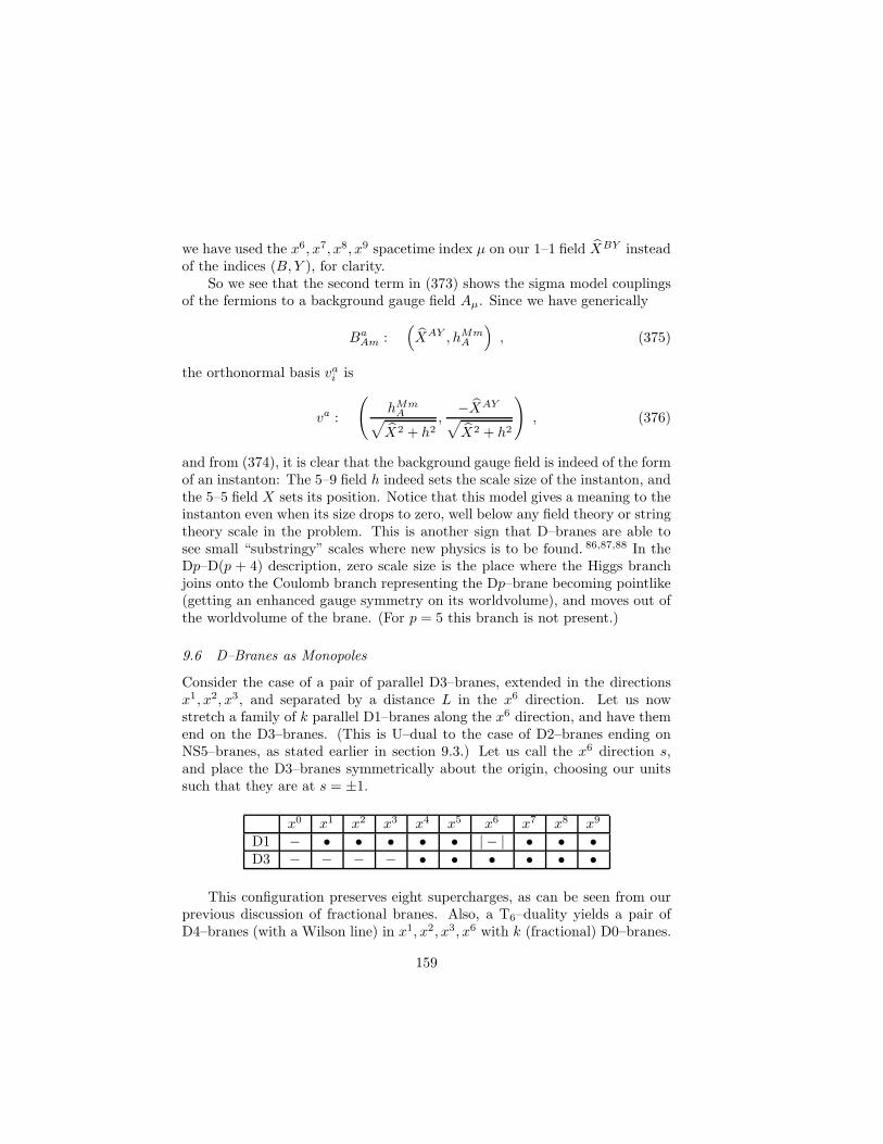
we have used the x6, x7, x8, x9 spacetime index µ on our 1–1 field XBY insteadof the indices (B, Y ), for clarity.

So we see that the second term in (373) shows the sigma model couplingsof the fermions to a background gauge field Aµ. Since we have generically

BaAm :(XAY , hMm

A

), (375)

the orthonormal basis vai is

va :

(hMmA√

X2 + h2,

−XAY

√X2 + h2

), (376)

and from (374), it is clear that the background gauge field is indeed of the formof an instanton: The 5–9 field h indeed sets the scale size of the instanton, andthe 5–5 field X sets its position. Notice that this model gives a meaning to theinstanton even when its size drops to zero, well below any field theory or stringtheory scale in the problem. This is another sign that D–branes are able tosee small “substringy” scales where new physics is to be found. 86,87,88 In theDp–D(p + 4) description, zero scale size is the place where the Higgs branchjoins onto the Coulomb branch representing the Dp–brane becoming pointlike(getting an enhanced gauge symmetry on its worldvolume), and moves out ofthe worldvolume of the brane. (For p = 5 this branch is not present.)

9.6 D–Branes as Monopoles

Consider the case of a pair of parallel D3–branes, extended in the directionsx1, x2, x3, and separated by a distance L in the x6 direction. Let us nowstretch a family of k parallel D1–branes along the x6 direction, and have themend on the D3–branes. (This is U–dual to the case of D2–branes ending onNS5–branes, as stated earlier in section 9.3.) Let us call the x6 direction s,and place the D3–branes symmetrically about the origin, choosing our unitssuch that they are at s = ±1.

x0 x1 x2 x3 x4 x5 x6 x7 x8 x9

D1 − • • • • • | − | • • •D3 − − − − • • • • • •

This configuration preserves eight supercharges, as can be seen from ourprevious discussion of fractional branes. Also, a T6–duality yields a pair ofD4–branes (with a Wilson line) in x1, x2, x3, x6 with k (fractional) D0–branes.

159

Insert 12: The Heterotic NS5–brane

Recall that in insert 11 (p.134) we deduced that there must be a solitonicbrane, the NS5–brane, which lives in SO(32) heterotic string theory. Thisfollowed from the fact the D5–brane of typeI had to map to such an ob-ject. This heterotic version of the NS5–brane inherits a number of propertiesfrom the D5–brane, the prinicipal one being that it must be an instanton ofthe SO(32) gauge theory of the heteroic string. In fact, it is the instantonproperty which led to its discovery early on. As a solution, it looks like thefollowing (to leading order in α′): 55,56

ds2 = ηµνdxµdxν + e2Φ

(drr + r2dΩ2

3

)

e2Φ = g2s

(1 + α′ (r

2 + 2ρ2)

(r2 + ρ2)2+ O(α′2)

), Hµνλ = −ǫ σ

µνλ ∂σΦ

Aµ =

(r2

r2 + ρ2

)g−1∂µg , g =

1

r

(x6 + ix7 x8 + ix9

x8 − ix9 x6 − ix7

), (377)

showing its structure as an SU(2) instanton localized in x6, x7, x8, x9, withscale size ρ. r2 is the radial coordinate, and dΩ2

3 is a metric on a round S3.

This arrangement was shown to preserve eight supercharges. (Also, we naivelyexpect that this construction should be related to our previous discussion ofinstantons, but instead of on IR4, they are on IR3 ×S1.) We can see it directlyfrom the fact that the presence of the D3– and D1–branes world–volumes placethe constraints:

ǫL = Γ0Γ1Γ2Γ3ǫR ; ǫL = Γ0Γ6ǫR , (378)

which taken together give eight supercharges, satisfying the condition

ǫL = Γ1Γ2Γ3Γ6ǫL . (379)

The 1–1 massless fields are simply the (1+1)–dimensional gauge field Aµ(t, s)and eight scalars Φm(t, s) in the adjoint of U(k), the latter representing thetransverse fluctuations of the branes. There are fluctuations in x1, x2, x3 andothers in x4, x5, x7, x8, x9. We shall really only be interested in the motionsof the D1–brane within the D3–brane’s directions x1, x2, x3, which is the“Coulomb branch” of the D1–brane moduli space. So of the Φm, we keeponly the three for m = 1, 2, 3. There are additionally 1–3 fields transforming inthe (±1, k). They form a complex doublet of SU(2)R and are 1 × k matrices.Crucially, these flavour fields are massless only at s = ±1, the locations wherethe D1–branes touch the D3–branes. If we were to write a Lagrangian for the

160

massless fields, there will be a delta function δ(s∓1) in front of terms contain-ing those. The structure of the Lagrangian is very similar to the one writtenfor the p − (p + 4) system, with the additional features of U(k) non–abelianstructure. Asking that the D–terms vanish, for a supersymmetric vacuum, weget: 175

dΦi

ds− [As,Φ

i] +1

2ǫijk[Φj ,Φk] = 0 , (380)

where we have ignored possible terms on the right hand side supported only ats = ±1. These would arise from the interactions induced by massless 1–3 fieldsthere. 176 We shall derive those effects in another way by carefully consideringthe boundary conditions in a short while.

If we choose the gauge in which As = 0, our equation (380) can be recog-nised as the Nahm equations, 184 known to construct the moduli space 186 ofN SU(2) monopoles, via an adaptation of the ADHM construction.174 The co-variant form As 6= 0, is useful for actually solving for the metric on the modulispace of monopole solutions and for the spacetime monopole fields themselves,as we shall show. 177

If our k D1–branes were reasonably well separated, we would imagine thatthe boundary condition at s = ±1 is clearly 2πα′Φi(s = 1)) = diagxi1, xi2, · · · , xik,where xin, i = 1, 2, 3 are the three coordinates of the end of the nth D1–brane(similarly for the other end). In other words, the off–diagonal fields corre-sponding to the 1–1 strings stretching between the individual D1–branes areheavy, and therefore lie outside the description of the massless fields. However,this is not quite right. In fact, it is very badly wrong. To see this, note thatthe D1–branes have tension, and therefore must be pulling on the D3–brane,deforming its shape somewhat. In fact, the shape must be given, to a goodapproximation, by the following description. The function s(x) describing theposition of the D3–brane along the x6 direction as a function of the three co-ordinates xi should satisfy the equation ∇2s(x) = 0, where ∇2 is the threedimensional Laplacian. A solution to this is

s = 1 +c

|x − x0|, (381)

where 1 is the position along the s direction and c and x0 are constants. So,far away from x0, we see that the solution is s = 1, telling us that we havea description of a flat D3–brane. Nearer to x0, we see that s increases awayfrom 0, and eventually blows up at x0.

We sketch this shape in figure 32(a). It is again our BIon–type solution,described before in section 4.6. The D3–brane smoothly interpolates betweena pure D1–brane geometry far away and a spiked shape resembling D1–brane

161

iX

s

(a) (b) (c)

Figure 32: (a): A D3–brane (vertical) with a D1–brane ending on it (horizontal) is actuallypulled (b) into a smooth interpolating shape. (c): Finitely separated D1–branes can only bedescribed with non–commutative coordinates (see text)

behaviour at the centre. A multi–centred solution is easy to construct asa superposition of harmonic solutions of the above type. Considering twoof them, we see that in fact for any finite separation of the D1–branes (asmeasured far enough along the s–direction), by time we get to s = 1, they willbe arbitrarily close to each other (see 32(b)). We therefore cannot forget 179

about the off–diagonal parts of Φm corresponding to 1–1 strings stretchingbetween the branes, and in fact we are forced to describe the geometry of thebranes’ endpoints on the D3–brane using non–abelian Xm. This is anotherexample of the “natural” occurrence of a non–commutativity arising in whatwe would have naively interpreted as ordinary spacetime coordinates.

We can see precisely what the boundary conditions must be, since we aresimply asking that there be a pole in Φi(s) as s→ ±1:

Φi(s) → Σi

s∓ 1, (382)

and placing this into (380), we see that the k×k residues must satisfy

[Σi,Σj ] = 2iǫijkΣk . (383)

In other words, they must form an k–dimensional representations of SU(2)!This representation must be irreducible, as we have seen. Otherwise it neces-sarily captures only the physics of m infinitely separated clumps of D1–branes,for the case where the representation is reducible into m smaller irreduciblerepresentations.

162

The problem we have constructed is that of monopoles 182,183 of SU(2)spontaneously broken to U(1) via an adjoint Higgs field H. 185 Ignoring thecentre of mass of the D3–brane pair, this SU(2) is on their world volume,and the separation is given by the vev, H of the Higgs field. The first order“Bogomol’nyi” equations 51 are:

Bi ≡1

2ǫijkFjk = DiH , with

Fij = ∂iAj − ∂jAi + [Ai, Aj ]; DiH = ∂iH + [Ai,H] , (384)

with gauge invariance (g(x) ∈ SU(2)):

Ai → g−1Aig + g−1∂ig; H → g−1Hg . (385)

Static, finite energy monopole solutions satisfy

‖H(x)‖ ≡ 1

2Tr [H∗H] → H as r → ∞ , (386)

where x = (x1, x2, x3), r2 = x2

1 + x22 + x2

3, and (2πα′)H = L/2, where L is theseparation of our D3–branes. The topological magnetic charge the monopolescarry comes from the fact that the vacuum manifold, which is SU(2)/U(1) ∼S2, can wind an integer number of times around the S2 at infinity, giving astable solution whose charge is a fixed number times that integer.

In fact, we can construct the Higgs field and gauge field of monopolesolution of the 3+1 dimensional gauge theory as follows. Given k×k Nahmdata (Φ1,Φ2,Φ3) = 2πα′(T1, T2, T3) solving the equation (380), there is anassociated differential equation for a 2k component vector v(s):

12N

d

ds+

(xa

21k + iTa

)⊗ σa

v = 0 .

There is a unique solution normalisable with respect to the inner product

< v1,v2 >=

∫ 1

−1

v†1v2ds .

In fact, the space of normalisable solutions to the equation is four dimensional,or complex dimension 2. Picking an orthonormal basis v1, v2, we constructthe Higgs and gauge potential as:

H = i

[< sv1, v1 > < sv1, v2 >< sv2, v1 > < sv2, v2 >

],

Ai =

[< v1, ∂iv1 > < v1, ∂iv2 >< v2, ∂iv1 > < v2, ∂iv2 >

](387)

163

The reader may notice a similarity between this means of extracting the gaugeand Higgs fields, and the extraction (373)(374) of the instanton gauge fieldsin the previous section. This is not an accident. The Nahm construction is infact a hyperKahler quotient which modifies the ADHM procedure. The factthat this arrangement of branes is T–dual to that of the p–(p + 4) system isthe physical realisation of this fact, showing that the basic families of hyper-multiplet fields upon which the construction is based (in the brane context)are present here too.

It is worth studying the case k = 1, for orientation. In this case, thesolutions Ti are simply real constants (2πα′)Φi = −iai/2, having the meaningof the position of the monopole at x = (a1, a2, a3). Let us place it at theorigin. Furthermore, as this situation is spherically symmetric, we can writex = (0, 0, r). Writing components v = (w1, w2), we get a pair of simpledifferential equations with solution

w1 = c1e−rs/2 , w2 = c2e

rs/2 . (388)

An orthonormal basis is given by

v1 :

(c1 = 0 , c2 =

√r

e2r − 1

); v2 :

(c2 = 0 , c1 =

√r

1 − e−2r

)(389)

and the Higgs field is simply:

H(r) = xiσiϕ(r)

r, with

ϕ(r) =r

(e2r − 1)

∫ 1

−1

sersds = r coth r − 1 . (390)

(here x = (0, 0, 1)) while the gauge field is:

Ai(r) = ǫijkσj xksinh r − r

r2 sinh r. (391)

This is the standard one–monopole solution of Bogomol’nyi, Prasad and Som-merfield, the prototypical “BPS monopole”. 51,52 We can insert the requireddimensionful quantities:

ϕ(r) → ϕ (Lr/4πα′) , (392)

to get the Higgs field:

H =σ3

rϕ

(Lr

4πα′

)−→ L

4πα′σ3 , as r → ∞ , (393)

164

showing the asymptotic positions of the D3–branes to be ±L/2, after multiply-ing by 2πα′ to convert the Higgs field (which has dimensions of a gauge field)to a distance in x6. A picture of the resulting shape 49,195 of the D3–brane isshown in figure 33.

0

0

–1

0

1

Figure 33: (a): A slice through part of two (horizontal) D3–branes with a (vertical) D1–braneacting as a single BPS monopole. This is made by plotting the exact BPS solution.

There is also a simple generalisation of the purely magnetic solution whichmakes a “dyon”, a monopole with an additional n units of electric charge. Itinterpolates between the magnetic monopole behaviour we see here and thespike electric solution we found in section 4.6. It is amusing to note 40 that anevaluation of the mass of the solution gives the correct formula for the boundstate mass of a D1–string bound to n fundamental strings, as it should, sincean electric point source is in fact the fundamental string.

10 D–Branes and Geometry II

10.1 The Geometry produced by D–Branes

By studying the supergravities arising in the low energy limit of the superstringtheory, it was shown that there exist extended solutions resembling general-isations of charged black holes. The p dimensional extended solution carriescharges under the R–R form C(p+1). The extremal cases are BPS solutions,and they differ from Reissner–Nordstrom black holes in that their horizons at

165

extremality have zero area p. The BPS (extremal) solution is: 78,79

ds2 = Z−1/2p ηµνdx

µdxν + Z1/2p dxidxi ,

e2Φ = g2sZp

(3−p)2 ,

C(p+1) = (Zp−1 − 1)g−1

s dx0 ∧ · · · ∧ dxp , (394)

where µ = 0, . . . , p, and i = p+ 1, . . . , 9, and the harmonic function Zp is

Zp = 1 +dp(2π)p−2gsNα

′(7−p)/2

r7−p; dp = 27−2pπ

9−3p2 Γ

(7 − p

2

). (395)

More complicated supergravity solutions preserving fewer supersymmetries (inthe extremal case) can be made by combining these simple solutions in variousways, by intersecting them with each other, boosting them to finite momentum,and by wrapping, and/or warping them on compact geometries. This allows forthe construction of finite area horizon solutions, corresponding to R–R chargedReissner–Nordstrom black holes, and generalisations thereof.

These solutions are R–R charged, but we have already established to all or-ders in string perturbation theory that Dp–brane actually are the basic sourcesof these R–R fields. In fact, the solutions (394) are normalised such that theycarry N units of the basic D–brane charge µp.

It is natural to suppose that there is a connection between these two fam-ilies of objects: Perhaps the solution (394) is “made of D–branes” in the sensethat it is actually the field due to N Dp–branes, all located at r = 0. This isprecisely how we are to make sense of this solution as a supergravity soliton so-lution. We must do so, since (except for p = 3) the solution is actually singularat r = 0, and so one might have simply discarded them as pathological, sincesolitons “ought to be smooth”, like the NS5–brane solution q. However, stringduality forces us to consider them, since smooth NS–NS solitons of variousextended sizes (which can be made by wrapping or warping NS5–branes in anarbitrary compactification) are mapped 196 into these R–R solitons under it,generalizing what we have already seen in ten dimensions (see e.g. insert 11,

pThis latter fact is interesting, but we will leave it to the reader to consult the lectures ofAmanda Peet203 and Mike Duff204 to see how this relates to the understanding of black holeentropy via D–branes, 202,205 and the AdS/CFT correspondence.qAt r = 0, the NS5–brane geometry (see (396)) opens up into an infinite throat geome-try, which is smooth, being IR7×S3, with a dilaton which is linear in the distance downone of the IR7 directions. The p = 3 version of the geometry in (394) also has a smooththroat, but the geometry is AdS5×S5, with constant dilaton. String theory propagatingon these throat backgrounds is, in each case, believed to be dual to a non–gravitationaltheory.197,198,199,200,201

166

Insert 13: The Type II NS5–brane

In insert 11 (p.134) we deduced that there must be a solitonic brane, theNS5–brane, in type II string theory. We can deduce its supergravity fieldsby using the ten dimensional S–duality transformations to convert the casep = 5 of equations (394), (395), to give: 55,56

ds2 = −dt2 + (dx1)2 + · · · + (dx5)2 + Z5

(drr + r2dΩ2

3

)

e2Φ = g2s Z5 = g2

s

(1 +

α′N

r2

),

B(6) = (Z−15 − 1)gsdx

0 ∧ · · · ∧ dx5 . (396)

This solution has N units of the basic magnetic charge of B(2), and is a pointin x6, x7, x8, x9. Here, r2 is the radial coordinate, and dΩ2

3 is a metric on around S3. The tension of this BPS object was deduced in insert 11 (p.134)to be: τF

5 = (2π)−5α′−3g−2s . (Note that the same transformation will give

a solution for the fields around a fundamental IIB string, by starting withthe p = 1 case of (394). 134,135) Recall also that we deduced the structure ofthis solution already using (a cavalier) T–duality to an ALE space in section9.3. Here, we have used S–duality to the precise D–brane computations tosee that our normalisations in those sections were correct.

(p.134)). With the understanding that there are D–branes “at their core”,which fits with the fact that they are R–R charged, they make sense of thewhole spectrum of extended solitons in string theory.

Let us build up the logic of how they can be related to D–branes. Recallthat the form of the action of the ten dimensional supergravity with NS–NSand R–R field strengths H and G respectively is, roughly:

S =

∫d10x

(e−2ΦR− e−2ΦH2 −G2

). (397)

There is a balance between the dilaton dependence of the NS–NS and gravi-tational parts, and so the mass of a soliton solution 79 carrying NS–NS charge(like the NS5–brane) scales like the action: TNS ∼ e−2Φ ∼ g−2

s . A R–R chargedsoliton has, on the other hand, a mass which goes like the geometric mean ofthe dilaton dependence of the R–R and gravitational parts: TR ∼ e−Φ ∼ g−1

s .This is just the behaviour we saw for the tension of the Dp–brane, computedin string perturbation theory, treating them as boundary conditions.

Dp–branes have been treated so far largely as point–like (in their transversedimensions) in an otherwise flat spacetime, and we were able to study an

167

arbitrary number of them by placing the appropriate Chan–Paton factors intoamplitudes. However, the solutions (394) have non–trivial spacetime curvature,and is only asymptotically flat. How are these two descriptions related?

The point is as follows: For every Dp–brane which is added to a situation,another boundary is added to the problem, and so a typical string diagram hasa factor gsN since every boundary brings in a factor gs and there is the traceover the N Chan–Paton factors. So perturbation theory is good as long asgsN < 1. Notice that this is the regime where the supergravity solution (394)fails to be valid, since the curvatures are high. On the other hand, for gsN > 1,the supergravity solution has its curvature weakened, and can be considered asa workable solution. This regime is where the Dp–brane perturbation theory,on the other hand, breaks down.

So we have a fruitful complementarity between the two descriptions. Inparticular, since we are only really good at string perturbation theory, i.e.gs < 1, for most computations, we can work with the supergravity solutionwith the interpretation that N is very large, such that the curvatures aresmall. Alternatively, if one restricts oneself to studying only the BPS sector,then one can work with arbitraryN , and extrapolate results —-computed withthe D–brane description for small gs— to the large gs regime, (since there areoften non–renormalisation theorems which apply) where they can be relatedto properties of the non–trivial curved solutions. This is the basis of thesuccessful statistical enumeration of the entropy of black holes, for cases wherethe solutions (394) are used to construct R–R charged black holes. 202,205 Thisexciting subject will be described in the notes of Amanda Peet. 203

In summary, for a large enough number of coincident D–branes or forstrong enough string coupling, one cannot consider them as points in flat space:they deform the spacetime according to the geometry given in eqn. (394).Given that D–branes are also described very well at low energy by gauge the-ories, this gives plenty of scope for finding a complementarity between de-scriptions of non–trivially curved geometry and of gauge theory. This is thebasis of what might be called “gauge theory/geometry” correspondences. Insome cases, when certain conditions are satisfied, there is a complete decou-pling of the supergravity description from that of the gauge theory, signallinga complete duality between the two. This is the basis of the AdS/CFT corre-spondence, 199,200 aspects of which are described in the lectures of Mike Duffand others.

168

10.2 Probing D–Branes’ Geometry with D–Branes: p with Dp

In the last section, we argued that the spacetime geometry given by equations(394) represents the spacetime fields produced by N Dp–branes. We notedthat as a reliable (or “trustworthy”) solution to supergravity, the product gsNought be be large enough that the curvatures are small. This correspondsto either having N small and gs large, or vice–versa. Since we are good atstudying situations with gs small, we can safely try to see if it makes sense tomake N large.

One way to imagine that this spacetime solution came about at weakcoupling was that we built it by bringing in N Dp–branes, one by one, frominfinity. If this is to be a sensible process, we must study whether it is reallypossible to do this. Imagine that we have been building the geometry for awhile, bringing up one brane at a time from r = ∞ to r = 0. Let us nowimagine bringing the next brane up, in the background fields created by all theother N branes. Since the branes share p common directions where there is nostructure to the background fields, we can ignore those directions and see thatthe problem reduces to the motion of a test particle in the transverse 9 − pspatial directions. What is the mass of this particle, and what is the effectivepotential that it moves in?

This sort of question is answered by the still–developing toolbox whichcombines the fact that we have a gauge theory on D–branes with the fact thatthe probe brane is a heavy object which can examine many distance scales,and has seen many applications in our understanding of spacetime geometryin various situations. 86,87,88,207,208,209

We can derive the answers to all of the present questions by deriving an ef-fective Lagrangian for the problem which results from the world–volume actionof the brane. We can exploit the fact that we have spacetime Lorentz trans-formations and world–volume reparametrisations at our disposal to choose thework in the “static gauge”. In this gauge, we align the world–volume coordi-nates, ξa, of the brane with the spacetime coordinates such that:

ξ0 = x0 = t ;

ξi = xi ; i = 1 · · · p ,ξm = ξm(t) ; m = p+ 1 · · · 9 . (398)

The Dirac–Born–Infeld part of the action (207) requires the insertion of theinduced metric derived from the metric in question. In static gauge, it is easy

169

to see that the induced metric becomes:

[G]ab =

G00 +∑

mnGmnvmvn 0 0 · · · 0

0 G11 0 · · ·...

......

. . ....

......

......

. . ....

0 0 0 · · · Gpp

, (399)

where vm ≡ dxm/dξ0 = xm.In our particular case of a simple diagonal metric, the determinant turns

out as

det[−Gab] = Z− (p+1)

2p

(1 − Zp

9∑

m=p+1

v2m

)= Z

− (p+1)2

p

(1 − Zpv

2). (400)

The Wess–Zumino term representing the electric coupling of the brane is, inthis gauge:

µp

∫C(p+1) = µp

∫dp+1ξ [C(p+1)]µ0µ1...µp

∂xµ0

∂ξa0

∂xµ1

∂ξa1· · · ∂x

µp

∂ξap

= µpVp

∫dt[Z−1p − 1

]g−1 , (401)

where Vp =∫dpx, the spatial world–volume of the brane. Now, we are going

to work in the approximation that we bring the branes slowly up the the mainstack of branes so we keep the velocity v small enough such that only termsup to quadratic order in v are kept in our computation. We can therefore theexpand the square root of our determinant, and putting it all together (notforgetting the crucial insertion of the background functional dependence of thedilaton from (394)) we get that the action is:

S = µpVp

∫dt

(−g−1

s Z−1p +

1

2gsv2 + g−1

s Z−1p − g−1

s

)

=

∫dtL =

∫dt

(1

2mpv

2 −mp

), (402)

which is just a Lagrangian for a free particle moving in a constant potential,(which we can set to zero) where mp = τpVp is the mass of the particle.

This result has a number of interesting interpretations. The first is simplythat we have successfully demonstrated that our procedure of “building” our

170

geometry (394) by successively bringing branes up from infinity to it, one at atime, makes sense: There is no non–trivial potential in the effective Lagrangianfor this process, so there is no force required to do this; correspondingly thereis no binding energy needed to make this system.

That there is no force is simply a restatement of the fact that these branesare BPS states, all of the same species. This manifests itself here as the factthat the R–R charge is equal to the tension (with a factor of 1/gs), saturatingthe BPS bound. It is this fact which ensured the cancellation between the r–dependent parts in (402) which would have otherwise resulted in a non–trivialpotential U(r). (Note that the cancellation that we saw only happens at orderv2 —the slow probe limit. Beyond that order, the BPS condition is violated,since it really only applies to statics.)

10.3 The Metric on Moduli Space

All of this has pertinent meaning from the point of view of field theory as well.Recall that there is a U(N) (p + 1)–dimensional gauge theory on a family ofN Dp–branes. Recall furthermore that there is a sector of the theory whichconsists of a family of (9− p) scalars, Φm, in the adjoint. Geometrically, theseare the collective coordinates for motions of the branes transverse to theirworld–volumes. Classical background values for the fields, (defining vacuaabout which we would then do perturbation theory) are equivalent to dataabout how the branes are distributed in this transverse space. Well, we havejust confirmed that there is in fact a “moduli space” of inequivalent vacua ofthe theory corresponding to the fact that one can give a vacuum expectationvalue to a component of an Φm representing, representing a brane moving awayfrom the clump of N branes. That there is no potential translates into thatfact that we can place the brane anywhere in this transverse clump, and it willstay there.

It is also worth noting that this metric on the moduli space is flat; treatingthe fields Φm as coordinates on the space IR9−p, we see (from the fact that thevelocity squared term in (402) appears as v2 = δmnv

mvn) that the metric seenby the probe is simply

ds2 ∼ δmndΦmdΦn . (403)

This flatness is a consequence of the high amount of supersymmetry (16 super-charges). For the case of D3–branes (whether or not they are in the AdS5×S5

limit), this result translates into the fact there that there is no running of thegauge coupling g2

YM of the superconformal gauge theory on the brane. This isread off from the prefactor g−2

YM = τ3(2πα′)2 = (2πgs)

−1 in the metric. Thesupersymmetry ensures that any corrections which could have been generated

171

are zero. We shall now see a less trivial version, where we have a nontrivialmetric in the case of eight supercharges.

10.4 Probing D–Branes’ Geometry with D–Branes: p with D(p− 4).

Let us probe the geometry of the p–branes with a D(p − 4)–brane. From ouranalysis of section 7, we know that this system is supersymmetric. Therefore,we expect that there should still be a trivial potential for the result of the probecomputation, but there is not enough supersymmetry to force the metric tobe flat. There are actually two sectors within which the probe brane canmove transversely. Let us choose static gauge again, with the probe aligned sothat its p− 4 spatial directions ξ1 − ξp−4 are aligned with the directions x1 −xp−4. Then there are four transverse directions within the p–brane background,labelled xp−3 − xp, and which we can call xi‖ for short. There are 9 − premaining transverse directions which are transverse to the p–brane as well,labelled xp+1 − x9 which we’ll abbreviate to xm⊥ . The 6–2 case is tabulated asa visual guide:

x0 x1 x2 x3 x4 x5 x6 x7 x8 x9

D2–brane − − − • • • • • • •6–brane − − − − − − − • • •

Following the same lines of reasoning as above, the determinant whichshall go into our Dirac–Born–Infeld Lagrangian is:

det[−Gab] = Z−

(p−3)2

p

(1 − v2

‖ − Zpv2⊥

), (404)

where the velocities come from the time (ξ0) derivatives of x‖ and x⊥. This isnice, since in forming the action by multiplying by the exponentiated dilatonfactor and expanding in small velocities, we get the Lagrangian

L =1

2mp−4

(v2‖ + Zpv

2⊥ − 2

), (405)

which again has a constant potential which we can discard, and pure kineticterms. We see that there is a purely flat metric on the moduli space for themotion inside the four dimensions of the p–brane geometry, while there is ametric

ds2 = Zp(r)δmndxmdxn , (406)

for the transverse motion. This is the Coulomb branch, in gauge theory terms,and the flat metric was on the Higgs branch. (In fact, the Higgs result does

172

not display all of the richness of this system that we have seen. In addition tothe flat metric geometry inside the brane that we see here, there is additionalgeometry describing the Dp–D(p−4) fields corresponding to the full instantongeometry. This “Yang–Mills geometry” comes from the fact that the D(p−4)–brane behaves as an instanton of the non–abelian gauge theory on the world–volume of the coincident Dp–branes.)

Notice that for the fields we have studied, we obtained a trivial potentialfor free without having to appeal to a cancellation due to the coupling of thecharge µp−4 of the probe. This is good, since there is no electric source of thisin the background for it to couple to. Instead, the form of the solution for thebackground makes it force–free automatically.

10.5 D2–branes and 6–branes: Kaluza–Klein Monopoles and M–Theory

Actually, when p ≥ 5, something interesting happens. The electric source ofC(p+1) potential in the background produces a magnetic source of C(7−p). Therank of this is low enough for there to be a chance for the D(p−4)–probe braneto couple to it even in the Abelian theory. For example, for p = 5 there is amagnetic source of C2 to which the D1–brane probe can couple. Meanwhile forp = 6, there is a magnetic source of C1. The D2–brane probes see this in aninteresting way. Let us linger here to study this case a bit more closely. Sincethere is always a trivial U(1) gauge field on the world volume of a D2–braneprobe, corresponding to the centre of mass of the brane, we should include thecoupling of the world–volume gauge potential Aa (with field strength Fab) toany of the fields coming from the background geometry.

In fact, as we saw before in section 6.2 there is a coupling

2πα′µ2

∫

M

C1 ∧ F , (407)

where C1 = Cφdφ is the magnetic potential produced by the 6–brane back-ground geometry, which is easily computed to be: Cφ = −(r6/gs) cos θ, wherer6 = gNα′1/2/2.

This extra degree of freedom on the world volume is equivalent to onescalar, since it comes from a gauge field in three dimensions. In our compu-tations we may exchange Aa for a scalar s, by Hodge duality in the (2+1)–dimensional world-volume. (This is of course a feature specific to the p=2case.)

To get the coupling for this extra scalar correct, we should augment theprobe computation. As we have seen, the Dirac–Born–Infeld action is modified

173

by an extra term in the determinant:

− detgab → −det(gab + 2πα′Fab) . (408)

We can 118,141 introduce an auxiliary vector field va, replacing 2πα′Fab bye2φµ−2

2 vavb in the Dirac action, and adding the term 2πα′∫MF ∧ v overall.

Treating va as a Lagrange multiplier, the path integral over va will give theaction involving F as before. Alternatively, we may treat Fab as a Lagrangemultiplier, and integrating it out enforces

ǫabc∂b(−µ2Cc + vc) = 0 . (409)

Here, Cc are the components of the pullback of C1 to the probe’s world–volume.The solution to the constraint above is

− µ2Ca + va = ∂as , (410)

where s is our dual scalar. We may now replace va by ∂as+µ2Ca in the action.The static gauge computation picks out only s+µ2Cφφ, and recomputing

the determinant gives

det = Z− 3

26

(1 − v2

‖ − Z6v2⊥ − Z

126 e

2Φ

µ22

[s+ µ2Cφφ

]2). (411)

Again, in the full Dirac–Born–Infeld action, the dilaton factor cancels theprefactor exactly, and including the factor of −µ2 and the trivial integral overthe worldvolume directions to give a factor V2, the resulting Lagrangian is

L =1

2m2(v

2‖ − 2) +

1

2V2

(µ2Z6

gv2⊥ +

gsµ2Z6

(s+ µ2Cφφ

)2), (412)

which is (after ignoring the constant potential) again a purely kinetic la-grangian for motion in eight directions. There is a non–trivial metric in thepart transverse to both branes:

ds2 = V (r)(dr2 + r2dΩ2

)+ V (r)−1 (ds+Aφdφ)2 ,

with V (r) =µ2Z6

gsand A =

µ2r6gs

cos θdφ , (413)

where dΩ2 = dθ2 + sin2θ dφ2. There is a number of fascinating interpretationsof this result. In pure geometry, the most striking feature is that there arenow eleven dimensions for our spacetime geometry. The D2–brane probe com-putation has uncovered, in a very natural way, an extra transverse dimension.

174

This extra dimension is compact, since s is periodic, which is inherited fromthe gauge invariance of the dual world–volume gauge field. The radius of theextra dimension is proportional to the string coupling, which is also interest-ing. This eleventh dimension is of course the M–direction we saw earlier. TheD2–brane has revealed that the six–brane is a Kaluza–Klein monopole 138 ofeleven dimensional supergravity on a circle, 126 which is constructed out of aTaub–NUT geometry (413). This fits very well with the fact that the D6 is theHodge dual of the D0–brane, which we already saw is a Kaluza–Klein electricparticle.

10.6 The Metric on Moduli Space

As before, the result also has a field theory interpretation. The (2 + 1)–dimensional U(1) gauge theory (with eight supercharges) on the worldvolumeof the D2–brane has Nf = N extra hypermultiplets coming from light stringsconnecting it to the Nf = N D6–branes. The SU(Nf) symmetry on theworldvolume of the D6–branes is a global “flavour” symmetry of the U(1)gauge theory on the D2–brane. A hypermultiplet Ψ has four components Ψi

corresponding to the 4 scalar degrees of freedom given by the four positionsΨi ≡ (2πα′)−1xi‖. The vector multiplet contains the vector Aa and three

scalars Φm ≡ (2πα′)−1xm⊥ . The Yang–Mills coupling is g2YM = gsα

′−1/2.

The branch of vacua of the theory with Ψ 6= 0 is called the “Higgs” branchof vacua while that with Φ 6= 0 constitutes the “Coulomb” branch, since thereis generically a U(1) left unbroken. There is a non–trivial four dimensionalmetric on the Coulomb branch. This is made of the three Φm, and the dualscalar of the U(1)’s photon. Let us focus on the quantities which survive in thelow energy limit α′ → 0 and hold fixed any sensible gauge theory quantitieswhich appear in our expressions. (Such procedures will be studied a lot in otherlecture courses in this school). The metric which appears in (413) survives thelimit as

ds2 = V (U)(dU2 + U2dΩ22) + V (U)−1(dσ +Aφdφ)2

where V (U) =1

4π2g2YM

(1 +

g2YMNf2U

); Aφ =

Nf8π2

cos θ , (414)

where U = r/α′ has the dimensions of an energy scale in the gauge theory.Also, σ = α′s, and we will fix its period shortly.

In fact, the naive tree level metric on the moduli space is that on IR3×S1,of form ds2 = g−2

YMdx2⊥ + g2

YMdσ2. Here, we have the tree level and one loop

result: V (U) has the interpretation as the sum of the tree level and one–loop

175

correction to the gauge coupling of the 2+1 dimensional gauge theory.209 Notethe factor Nf in the one loop correction. This multiplicity comes from thenumber of hypermultiplets which can run around the loop. Similarly, the crossterm from the second part of the metric has the interpretation as a one–loopcorrection to the naive four dimensional topology, changing it to the (Hopf)fibred structure above.

Actually, the moduli space’s dimension had to be a multiple of four, asit generally has to be hyperKahler for D=2 + 1 supersymmetry with eightsupercharges. 151 Our metric is indeed hyperKahler since it is the Taub–NUTmetric: The hyperKahler condition on the metric in the form it is written isthe by–now familiar equation: ∇× A = ∇V (U), which is satisfied.

In fact, we are not quite done yet. With some more care we can establishsome important facts quite neatly. We have not been careful about the periodof σ, the dual to the gauge field, which is not surprising given all of the factorsof 2, π and α′. To get it right is an important task, which will yield interestingphysics. We can work it out in a number of ways, but the following is quiteinstructive. If we perform the rescaling U = ρ/4g2

YM and ψ = 8π2σ/Nf , ourmetric is:

ds2 =g2YM

64π2ds2TN , where

ds2TN =

(1 +

2Nfρ

)(dρ2 + ρ2dΩ2

2) + 4N2

(1 +

2Nfρ

)−1

(dψ + cos θdφ)2 ,

(415)

which is a standard form for the Taub–NUT metric, with mass Nf , equal to the“nut parameter” for this self–dual case. 152 This metric is apparently singularat ρ = 0, and in fact, for the correct choice of periodicity for ψ, this pointlikestructure, called a “nut”, is removable, just like the case of the bolt singularityencountered for the Eguchi–Hanson space. (See insert 10, p.102.) Just forfun, insert 14 (p.177) carries out the analysis and finds that ψ should haveperiod 4π, and so in fact the full SU(2) isometry of the metric is preserved.

What does this all have to do with gauge theory? Let us consider thecase of Nf = 1, which means one six brane. This is 2+1 dimensional U(1)gauge theory with one hypermultiplet, a rather simple theory. We see thatafter restoring the physical scales to our parameterers, our original field σ hasperiod 1/2π, and so we see that the dual to the photon is more sensibly definedas σ = 4π2σ, which would have period 2π, which is a more reasonable choicefor a scalar dual to a photon. We shall use this choice later. With this choice,the metric on the Coulomb branch of moduli space is completely non–singular,as should be expected for such a simple theory.

176

Insert 14: Removing the “Nut” Singularity from Taub–NUT

The metric (415) will be singular at at the point ρ = 0, for arbitrary period-icity of ψ. This will be a pointlike singularity which is called a “nut”, 65,64 incontrast to the “bolt” we encountered for the Eguchi–Hanson space in insert10 (p.102), which was an S2. In this case, near ρ = 0, if we make the spacelook like the origin of IR4, we can make this pointlike structure into nothingbut a coordinate singularity. Near ρ = 0, we have:

ds2TN =2Nfρ

(dρ2 + ρ2dΩ2

2 + ρ2(dψ + cos θdφ)2),

which is just the right metric for IR4 if ∆ψ = 4π, the standard choice forthe Euler coordinate. (This may have seemed somewhat heavy–handed fora result one would perhaps have guessed anyway, but it is worthwhile seeingit, in preparation for more complicated examples.)

Let us now return to arbitraryNf . This means that we have Nf hypermul-tiplets, but still a U(1) 2+1 dimensional gauge theory with a global “flavour”symmetry of SU(Nf ) coming from the six–branes. There is no reason for theaddition of hypermultiplets to change the periodicity of our dual scalar andso we keep it fixed and accept the consequences when we return to physicalcoordinates (U, σ): The metric on the Coulomb branch is singular at U = 0 !This is so because insert 14 told us to give σ a periodicity of 2πNf , but weare keeping it as 2π. So our metric in physical units has σ with period 2πappearing in the combination (2dσ+Nf cos θdφ)2. This means that the metricis no longer has an SU(2) acting, since the round S3 has been deformed intoa “squashed” S3, where the squashing is controlled by Nf . In fact, there is adeficit angle at the origin corresponding to an ANf−1 singularity.

How are we to make sense of this singularity? Well, happily, this all fitsrather nicely with the fact that for Nf > 1 there is an SU(Nf) gauge theory onthe sixbranes, and so there is a Higgs branch, corresponding to the D2-branebecoming an SU(Nf) instanton! The singularity of the Coulomb branch isindeed a signal that we are at the origin of the Higgs branch, and it also fitsthat there is no singularity for Nf = 1.

It is worthwhile carrying out this computation for the case ofNf D6–branesin the presence of a negative orientifold 6–plane oriented in the same way. Inthat case we deduce from facts we learned before that the presence of the O6–plane gives global flavour group SO(2Nf ) for Nf D6–branes. The D2–branehowever carries an SU(2) gauge group. This is T–dual to the earlier statement

177

made in section 9.4 about D9–branes in type I string theory carrying SO(Nf )groups while D5’s carry USp(2M) groups. 108,109: The orientifold forces a pairof D2–branes to travel as one, with a USp(2) = SU(2) group.

So the story now involves 2+1 dimensional SU(2) gauge theory with Nfhypermultiplets. The Coulomb branch for Nf = 0 must be completely non–singular, since again there is no Higgs branch to join to. This fits with thefact that there are no D6–branes; just the O6–plane. The result for the metricon moduli space can be deduced from a study of the gauge theory (with theintuition gained from this stringy situation), and has been proven to be theAtiyah–Hitchin manifold. 206,209,224,225 Some of this will be discussed in moredetail in subsection 10.8. For the case of Nf = 1, the result is also non–singular(there is again no Higgs branch for 1 D6–brane) and the result is a certain coverof the Atiyah–Hitchin manifold. 206,224. The case of general Nf gives certaingeneralisations of the Atiyah–Hitchin manifold.224,226 The manifolds haveDNf

singularities, consistent with the fact that there is a Higgs branch to connect to.Note also that a sringy interpretation of this result is that the strong couplinglimit of these O6–planes is in fact M–theory on the Atiyah–Hitchin manifold,just like it is Taub–NUT for the D6–brane. r

10.7 When Supergravity Lies: Repulson Vs. Enhancon

Despite the successes we have achieved in the previous section with interpreta-tion of supergravity solutions in terms of constituent D–branes, we should becareful, even in the case when we have supersymmetry to steer us away frompotential pathologies. It is not always case that if someone presents us with asolution of supergravity with R–R charges that we should believe that it hasan interpretation as being “made of D–branes”.

Consider again the case of eight supercharges. We studied brane config-urations with this amount of supersymmetry by probing the geometry of N(large) Dp–branes with a single D(p−4)–brane. As described in previous sec-tions, another simple way to achieve a geometry with eight supercharges fromD–branes is to simply wrap branes on a manifold which already breaks halfof the supersymmetry. The example mentioned was the four dimensional caseof K3. In this case, we learned that if we wrap a D(p+4)–brane (say) on K3,

rIt is amusing to note —and the reader may bave already spotted it— that the story aboveseems to be describing local pieces of K3, which has ADE singularities of just the right type,with the associated SU(N) and SO(2N) enhanced gauge symmetries appearing also (globalflavour groups for the 2+1 dimensional theory here). (The existence of three new exceptionaltheories, for E6, E7, E8, is then immediate. 209.) What we are actually recovering is thefact 127 that there is a strong/weak coupling duality between type I (or SO(32) heterotic)string theory on T 3 and M–theory on K3!!

178

we induce precisely one unit of negative Dp–brane charge 92 supported on theunwrapped part of the worldvolume (see eqn.(302)). At large N therefore,we might expect that there is a simple supergravity geometry which might beobtained by taking the solution for the D(p + 4)–Dp system, and modifyingthe asymptotic charges to suit this situation. The resulting geometry naivelyshould have the interpretation as that due to a large number N of wrappedD(p+4) branes:

ds2 = Z−1/22 Z

−1/26 ηµνdx

µdxν + Z1/22 Z

1/26 dxidxi + V 1/2Z

1/22 Z

−1/26 ds2K3 ,

e2Φ = g2sZp

(3−p)/2Zp+4−(p+1)/2 ,

C(p+1 ) = (Zp−1 − 1)g−1

s dx0 ∧ dx1 ∧ · · · ∧ dxp+1

C(p+5 ) = (Z−1p+4 − 1)g−1

s dx0 ∧ dx1 ∧ · · · ∧ dxp+5 . (416)

Here, µ, ν run over the x0 − xp+1 directions, which are tangent to all thebranes. Also i runs over the directions transverse to all branes, xp+2 − x5,and in the remaining directions, transverse to the induced brane but inside thelarge brane, ds2K3 is the metric of a K3 surface of unit volume. V is the volumeof the K3 as measured at infinity, but the supergravity solution adjusts itselfsuch that V (r)=V Zp/Zp+4 is the measured volume of the K3 at radius r.

Let us focus on the case p = 2, where we wrap D6–branes to get inducedD2–branes. s

x0 x1 x2 x3 x4 x5 x6 x7 x8 x9

D2 − − − • • • • • • •D6 − − − • • • − − − −K3 − − − − − − • • • •

The harmonic functions are

Z2 = 1 +r2r, r2 = − (2π)4gsNα

′5/2

2V,

Z6 = 1 +r6r, r6 =

gsNα′1/2

2, (417)

normalised such that the D2– and D6–brane charges are Q2=−Q6 = −N .Note that the smaller brane is delocalised in the K3 directions, as it should be,since the same is true of K3’s curvature.sThis will also teach us a lot about the pure SU(N) gauge theory on the remaining 2+1dimensional world–volume. Wrapping D7–branes (p = 3) teaches us 211 about pure SU(N)gauge theory in 3+1 dimensions, where we should make a connection to Seiberg–Wittentheory at large N . 212,213

179

We worked out the spectrum of type IIA supergravity theory compactifiedto six dimensions on K3 in subsection 5.5. The six dimensional supergravitytheory has as an additional sector twenty–four U(1)’s in the R–R sector. Ofthese, twenty–two come from wrapping the ten dimensional two–form on the19+3 two–cycles of K3. The remaining two are special U(1)’s for our purposes:One of them arises from wrapping IIA’s five–form entirely on K3, while thefinal one is simply the plain one–form already present in the uncompactifiedtheory.

It is easy to see that there is something wrong with the geometry whichwe have just written down, representing the wrapping of the D6–branes onthe K3. There is a naked singularity at r = |r2|, known as the “repulson”,since it represents a repulsive gravitational potential, 214 as can be seen byscattering test particles in to small enough r. The curvature diverges therewhich is related to the fact that the volume of the K3 goes to zero there, andthe geometry stops making sense. Let us look carefully to see if this is reallythe geometry produced by the branes. 211

The object we have made should be a BPS membrane made of N identicalobjects. These objects feel no force due to each other’s presence, and thereforethe BPS formula for the total mass is simply (see eqn.(303))

τN =N

gs(µ6V − µ2) (418)

with µ6 = (2π)−6α′−7/2 and µ2 = (2π)−2α′−3/2. In fact, the BPS membraneis actually a monopole of one of the six dimensional U(1)’s. It is obvious whichU(1) this is; the diagonal combination of the two special ones we mentionedabove. The D6–brane component is already a monopole of the IIA R–R one–form, and the D2 is a monopole of the five–form, which gets wrapped.

N.B.: As we shall see, the final combination is a non–singular BPS monopole,having been appropriately dressed 215 by the Higgs field associated to thevolume of K3. Also, it maps 196 (under the strong/weak coupling dualityof the type IIA string on K3 to the heterotic string on T 4) 125,127,72 to abound state of a Kaluza–Klein monopole 138 and an H–monopole 217, madeby wrapping the heterotic NS5–fivebrane. 211,218,219

If we are to interpret our geometry as having been made by bringing to-gether N copies of our membrane, we ought to be able to carry out the proce-dure we described in the previous sections. We should see that the geometryas seen by the probe is potential–free and well–behaved, allowing us the inter-pretation of being able to bring the probe in from infinity.

180

The effective action for a D6–brane probe (wrapped on the K3) is:

S = −∫

M

d3ξ e−Φ(r)(µ6V (r) − µ2)(− det gab)1/2 + µ6

∫

M×K3

C7 − µ2

∫

M

C3 .

(419)Here M is the projection of the world-volume onto the three non–compact di-mensions. As discussed previously (see eqn.(305) and surrounding discussion),the first term is the Dirac–Born–Infeld action with the position dependenceof the tension (418) taken into account; in particular, V (r) = V Z2(r)/Z6(r).The second and third terms are the couplings of the probe charges (µ6,−µ2)to the background R–R potentials, following from eqn (302), and surroundingdiscussion.

Having derived the action, the calculation proceeds very much as we out-lined in the previous sections, with the result:

L = −µ6V Z2 − µ2Z6

Z6Z2gs+µ6V

gs(Z−1

6 − 1) − µ2

gs(Z−1

2 − 1)

+1

2gs(µ6V Z2 − µ2Z6)v

2 +O(v4) . (420)

The position–dependent potential terms cancel as expected for a supersymmet-ric system, leaving the constant potential (µ6V −µ2)/g and a nontrivial metricon moduli space (the O(v2) part) as expected with eight supersymmetries. Themetric is proportional to

ds2 =1

gs(µ6V Z2 − µ2Z6) dx

2⊥ =

α′−3/2

(2π)2g

(V

V∗− 1− gsNα

′1/2

r

)(dr2 + r2dΩ2

2) .

(421)We assume that V > V∗ ≡ (2π)4α′2, so that the metric at infinity (and themembrane tension) are positive. However, as r decreases the metric eventuallybecomes negative, and this occurs at a radius

r =2V

V − V∗|r2| ≡ re (422)

which is greater than the radius rr = |r2| of the repulson singularity.In fact, our BPS monopole is becoming massless as we approach the special

radius. This should mean that the U(1) under which it is charged is becomingenhanced to a non–abelian group. This is the case. There is a purely stringyphenomenon which lies outside the W–bosons are wrapped D4–branes, whichenhance the U(1) to an SU(2). The masses of wrapped D4–branes is just like

181

that of the membrane, and so becomes zero when the K3’s volume reaches thevalue V∗≡(2π

√α′)4.

The point is that the repulson geometry represents supergravity’s bestattempt to construct a solution with the correct asymptotic charges. In thesolution, the volume of the K3 decreases from its asymptotic value V as oneapproaches the core of the configuration. At the centre, the K3 radius is zero,and this is the singularity. This ignores rather interesting physics, however.At a finite distance from the putative singularity (where VK3 = 0), the volumeof the K3 gets to V=V∗, so the stringy phenomena —including new masslessfields— giving the enhanced SU(2) should have played a role. t So the as-pects of the supergravity solution near and inside the special radius, called the“enhancon radius”, should not be taken seriously at all, since it ignored thisstringy physics.

To a first approximation, the supergravity solution should only be takenas physical down to the enhancon radius re. That locus of points, a two–sphereS2, is itself called an “enhancon”. 211

Note also that the size of the monopole is inverse to the mass of the Wbosons, and so in fact by time our probe gets to the enhancon radius, it hassmeared out considerably, and in fact merges into the geometry, forming a“shell” with the other monopoles at that radius. Since by this argument wecannot place sharp sources inside the enhancon radius, evidently, and so thegeometry on the inside must be very different from that of the repulson. Infact, to a first approximation, it must simply be flat, forming a smooth junctionwith the outside geometry at r = re.

In general, one expects the same sort of reasoning to apply for all p, andso the enhancon locus resulting from wrapping a D(p + 4)–brane on K3 isS4−p × Rp+1, whose interior is (5 + 1)–dimensional. For even p the theory inthe interior has an SU(2) gauge symmetry, while for odd p there is the A1 two–form gauge theory. The details of the smoothing will be very case dependent,and it should be interesting to work out those details.

One can also study SO(2N), SO(2N+1) and USp(2N) gauge theories witheight supercharges in various dimensions using similar techniques, placing anorientifold O6–plane into the system parallel to the D6–branes. The enhanconthen becomes an RP2. 220

Note that the Lagrangian (420) depends only on three moduli space coor-dinates, (x3, x4, x5), or (r, θ, φ) in polar coordinates. As mentioned before, a(2+1) dimensional theory with eight supercharges, should have a moduli space

tActually, this enhancement of SU(2) is even less mysterious in the heterotic–on–T 4 dualpicture mentioned two pages ago. 211 It is just the SU(2) of a self–dual circle in this picture,which we studied extensively in section 3.3

182

metric which is hyperKahler. 151 So we need at least one extra modulus, s. Asimilar procedure to that used in section 10.5 can be used to introduce thegauge field’s correct couplings and dualize to introduce the scalar s. A crucialdifference is that one must replace 2πα′Fab by e2φ(µ6V (r) − µ2)

−2vavb in theDirac–Born–Infeld action, the extra complication being due to the r dependentnature of the tension. The static gauge computation gives for the kinetic term:

L = F (r)(r2 + r2Ω2

)+ F (r)−1

(s/2 − µ2Cφφ/2

)2

, (423)

where

F (r) =Z6

2gs(µ6V (r) − µ2) , (424)

and Ω2 = θ2 + sin2θ φ2.

10.8 The Metric on Moduli Space

Again, there is gauge theory information to be extracted here. We have puregauge SU(N) theory with no hypermultiplets, and eight supercharges. Weshould be able to cleanly separate the gauge theory data from everything elseby taking the decoupling limit α′ → 0 while holding the gauge theory cou-pling g2

YM = g2YM,pV

−1 = (2π)4gsα′3/2V −1 and the energy scale U = r/α′

(proportional to MW ) fixed. In doing this, we get the metric:

ds2 = f(U)(U2 + U2dΩ2

)+ f(U)−1

(dσ − N

4π2Aφdφ

)2

,

where f(U) =1

4π2g2YM

(1 − g2

YMN

U

), (425)

the U(1) monopole potential is Aφ = ±1 − cos θ, and σ = sα′, and the metricis meaningful only for U>Ue = λ. This metric, which should be contrastedwith equation (414), is the hyperKahler Taub–NUT metric, but this time witha negative mass. This metric is singular, but the full metric, obtained byinstanton corrections to this one–loop result, should be smooth, as we willdiscuss. The details of this smoothing will teach us more about this p = 2case of the enhancon geometry and the interpolation between the exteriorsupergravity solution and the interior region, which is flat to leading order.

From the point of view of the monopole description, this manifold shouldbe related to the metric on the moduli space of monopoles. This fits withthe fact that the moduli space of the gauge theory and that of the monopoleproblem are known to be identified. 224,221,172 It is clearly a submanifold of

183

the full 4N−4 dimensional metric on the relative moduli space 186 of N BPSmonopoles which is known to be smooth.194 For the problem of two monopoles,that moduli space manifold222 is the Atiyah–Hitchin manifold, 206 while forgeneral N it is more complicated. This should remind the reader of our studyin subsection 10.6. Recalling that this is also a study of SU(N) gauge theorywith no hypermultiplets, we know the result for N = 2: The metric on themoduli space must be smooth, as there is no Higgs branch to connect to viathe singularity. This is true for all SU(N), and matches the monopole result.For N = 2, we saw that the metric on the moduli space is actually the Atiyah–Hitchin manifold.

The structure of our particular four dimensional submanifold of the generalmoduli space is very similar to that of an Atiyah–Hitchin manifold, in fact! Tosee this, 223 change variables in our probe metric (425) by absorbing a factor ofλ/2 = g2

YMN/2 into the radial variable U , defining ρ = 2U/λ. Further absorbψ = σ8π2/N and gauge transform to Aφ = − cos θ. Then we get:

ds2 =g2YMN

2

32π2ds2TN− , with (426)

ds2TN− =

(1 − 2

ρ

)(dρ2 + ρ2dΩ2

)+ 4

(1 − 2

ρ

)−1

(dψ + cos θdφ)2 .

The latter is precisely the form of the Taub–NUT metric that one gets byexpanding the Atiyah–Hitchin metric in large ρ and neglecting exponentialcorrections.u

Now for the same reasons as in subsection 10.6, the periodicity of σ is1/2π, and we will use σ = 4π2σ as our 2π periodic scalar dual to the photonon the probe’s world–volume. Looking at the choices we made above, thisimplies that for the SU(2) case, the coordinate ψ has period 2π ! This issurprising (perhaps), but does not lead to a “nut” singularity (see insert 14,p.177) for the following reason: The nut would be at ρ = 0, but there is a moredangerous singularity already at ρ = 2. This new singularity is an artifact ofa large ρ expansion, however. There is a unique and completely non–singularmanifold whose metric is as asymptotically close to ds2TN− up to exponentialcorrections, which is determined as follows:

In this case of N = 2, there is an SO(3) = SU(2)/ZZ2 isometry in the prob-lem, and not the naive SU(2) of the Taub–NUT space, since ψ has period 2πand not 4π. This isometry, smoothness, and the condition of hyperKahleritypick out uniquely the Atiyah–Hitchin manifold as the completion of the neg-ative mass Taub–NUT and completes the story for the SU(2) gauge theoryuThe reader should compare this result to that in equation (415) to see that it is the caseof N = −1, using the meaning that N has in subsection 10.6.

184

moduli space problem. 224 The Atiyah–Hitchin manifold can be written in thefollowing manifestly SO(3) invariant manner: 206,228

ds2AH = f2dρ2 + a2σ21 + b2σ2

2 + c2σ23 ;

2bc

f

da

dρ= (b − c)2 − a2 , and cyclic perms.; ρ = 2K

(sin

β

2

), (427)

where the choice f = −b/r can be made, the σi are defined in (264), and K(k)is the elliptic integral of the first kind:

K(k) =

∫ π2

0

(1 − k2 sin2 τ)12 dτ . (428)

Also, k= sin(β/2), the “modulus”, runs from 0 to 1, so π ≤ ρ ≤ ∞.In fact, the solution for a, b, c can be written out in terms of elliptic func-

tions, but we shall not do that here. It is enough to note that when ρ is large,the difference between this metric and ds2TN− is exponentially small in ρ. Theseexponential corrections for smaller ρ remove the singularity: ρ = 2 is just anartefact of the large ρ metric in the above form (427).

The exponential corrections have the expected interpretation in the gaugetheory as the instanton corrections. 225 Translating back to physical variables,we see that these corrections go as exp (−U/g2

YM), which has the correct formof action for a gauge theory instanton. (We have just described a cover of theAtiyah–Hitchin manifold needed for the SU(2) case. There is an additionalidentification to be discussed below.)

Can we learn anything from this for our case of general N , especially forlarge N , to teach us about the enhancon geometry? We have to be careful.Now, fixing our period of σ to be 2π as before, for general N the reultingperiod of ψ in the scaled variables is ∆ψ = 4π/N . Therefore our isometry isnot SO(3) but SU(2)/ZZN . (So the boundary at infinity is the squashed S3,given by S3/ZZN ).

So the manifold we need is not quite the Atiyah–Hitchin manifold, butprobably a close cousin; as the Atiyah–Hitchin manifold goes once around itsψ–circle, the manifold we need goes around N/2 times, and it is tempting towonder if the manifold we seek is simply a smooth quotient of it. It would beinteresting to find this manifold using requirements of uniqueness and smooth-ness. This manifod certainly exists, given the data that we have presentedfrom the point of view of the gauge theory and the monopole physics.

Once we have found this manifold in scaled coordinates, we can then rescaleeverything back to the original physical variables. The rescaled exponentialcorrections should be the gauge theory instanton corrections which we expect,

185

although for large N they will be quite small, and the dominant geometry willbe that of the negative mass Taub–NUT for a wide range of validity. 227

Even without precise knowledge of the manifold we seek, we can learnmuch about our problem at large N : We are working on a very symmetricsubspace of the full 4N−4 dimensional relative moduli space of monopoles. Theproblem is of a large charge N monopole being approached by a small charge 1monopole probe. The Atiyah–Hitchin manifold (N = 2) in standard variablesused in (427) and (427) represents two charge 1 monopoles approaching oneanother from asymptotic large relative separation ρ. We can borrows some ofthe intuitive behaviour of the two monopole case, some interpretation: For thetwo charge 1 case, for small ρ they begin to merge into a charge 2 monopole,and ρ no longer has distinct meaning as a separation. The singularity at ρ = 2is never reached, as it is an artifact of the large ρ expansion; instead ρ = π is thecase where the monopoles are coincident. It is a removable “bolt singularity”in the full Atiyah–Hitchin geometry, of exactly the type we saw in the case ofthe Eguchi–Hanson space in insert 10 (p.102).

Actually, we have described a trivial cover of the true Atiyah–Hitchinspace. The two monopole problem has an obvious ZZ2 symmetry coming fromthe fact that the monopoles are identical. Some field configurations describedby the manifold as described up to now are overcounted, and so we must divideby this ZZ2. The result is that the bolt is an RP2 instead of an S2. We willnot have such an identification for N > 2.

Note that when we scale ρ back to U , our coordinate U (for large U) is trulya radial coordinate, as one extremely heavy monopole is at the centre, beingprobed by a charge 1 monopole. The generalisation of the Atiyah–Hitchinbolt then represents the place of closest approach of the probe, where it hassmoothed out. This is the smoothed, “nonperturbative” enhancon locus.

11 D–Branes and Geometry III: Non–Commutativity

11.1 Open Strings with a Background B–Field

Let us return briefly to where we started out. Writing down the open stringsigma model (in conformal gauge). Gathering together the various pieces fromthe early chapters, we have:

S =1

4πα′

∫

Σ

d2σ(gabGµν(X) + ǫabBµν(X)

)∂aX

µ∂bXν+

∫

∂Σ

dτAi(X)∂τXi .

(429)We are going to focus on the case where we have some gauge field on theworld volume of a Dp–brane, which has world–volume coordinates X i, for

186

i = 0, . . . , p. Transverse coordinates are Xm, for m = p + 1, . . . , 9. We shallalso have, as usual a trivial background Gµν = ηµν ; Φ = constant, and aconstant background B field. We can go and vary the action as we did before,and we will find that again our Xµ’s satisfy the 2D wave equation, but we haveslightly different boundary conditions at σ = 0, π:

∂σXi + ∂τX

jF ij = 0 , Xm = xm0 , (430)

where we have written the gauge invariant combination F = B + 2πα′F . Thesecond part is the Dirichlet boundary condition, fixing xm0 as the positions ofthe Dp–brane.

Before going any further, it is worth trying to interpret the modificationto the Neumann boundary condition, in the light of what we already know.Let us choose two directions in which there are non trivial components of F ,let us say X1 and X2. So we have either non–zero B12 or F12, or both. Thenwriting out the condition, we have:

∂σX1 + ∂τX

2F12 = 0 ; (431)

∂σX2 − ∂τX

1F12 = 0 , (432)

where we have used the fact that F is antisymmetric. Now, if we write F12 =

cot θ, then we have

cos θ∂σX1 + sin θ∂τX

2 = 0 ; (433)

− sin θ∂τX1 + cos θ∂σX

2 = 0 . (434)

Now if we do a T–duality in the 2 direction, we exchange ∂σ and ∂τ ’s actionon X2. Then we see that we can rotate by an angle θ in the 1–2 plane, to newaxes X ′1, X ′2 to get:

∂σX′1 = 0 , ∂τX

′2 = 0 . (435)

Now, ∂τXa = 0 is not quite a Dirichlet condition in the direction Xa, but

nearly. Instead of saying that there is a definite position Xa = xa0 that thestring endpoint must be on, it is in fact a definite statement about the con-jugate momentum. So we interpret this to mean that there is a Dirichletcondition, but that the associated position has not been specified, and so itcan be anywhere in the direction Xa. So in fact, we have gone from a D2–brane filling the X1, X2 directions to a D–brane lying along the X ′1 direction(see figure 34(c)). Also, before rotation, we see that ∂σX

1 + tan θ∂σX2 = 0 is

simply specifying that there be a D1–brane lying at an angle θ in the 1–2 plane(See figure 34(b)). We saw this in previous sections, but it is worth repeating

187

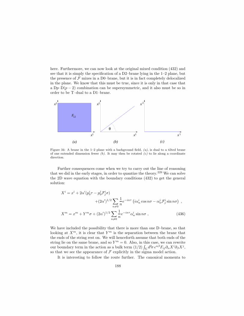
here. Furthermore, we can now look at the original mixed condition (432) andsee that it is simply the specification of a D2–brane lying in the 1–2 plane, butthe presence of F mixes in a D0–brane, but it is in fact completely delocalizedin the plane. We know that this must be true, since it is only in that case thata Dp–D(p− 2) combination can be supersymmetric, and it also must be so inorder to be T–dual to a D1–brane.

x1

x2

F12

x1

x2

x 1

θ

x 2

(a) (b) (c)

Figure 34: A brane in the 1–2 plane with a background field, (a), is dual to a tilted braneof one extended dimension fewer (b). It may then be rotated (c) to lie along a coordinatedirection.

Further consequences come when we try to carry out the line of reasoningthat we did in the early stages, in order to quantize the theory.229 We can solvethe 2D wave equation with the boundary conditions (432) to get the generalsolution:

X i = xi + 2α′(pi0τ − pj0F ijσ)

+(2α′)1/2∑

n6=0

1

ne−inτ

(iαin cosnσ − αjnF i

j sinnσ),

Xm = xm + Y mσ + (2α′)1/2∑

n6=0

1

ne−inταin sinnσ , (436)

We have included the possibility that there is more than one D–brane, so thatlooking at Xm, it is clear that Y m is the separation between the brane thatthe ends of the string rest on. We will henceforth assume that both ends of thestring lie on the same brane, and so Y m = 0. Also, in this case, we can rewriteour boundary term in the action as a bulk term (1/2)

∫Σd2σ ǫαβFij∂αX

i∂βXj,

so that we see the appearance of F explicitly in the sigma model action.

It is interesting to follow the route further. The canonical momenta to

188

Xµ’s are

Πm =1

2πα′∂τX

i ; Πi =1

2πα′

(∂τX

i + ∂σXjF i

j

), (437)

from which we can compute the total conserved momentum:

Pmtot = 0 ; P itot =

∫ π

0

dσΠi(τ, σ) = pj0Mij , (438)

where

Mij = ηij −Fki Fkj . (439)

The Hamiltonian is then, using equations (59,60):

H =1

2

Mijp

i0pj0 +

∑

n6=0

(Mijαinα

j−n + αmn α

m−n)

, (440)

where we can see the non–trivial modification in the directions parallel to thebrane, and nowhere else.

11.2 Non–Commutative Geometry and D–branes

Now the fun comes when we try to quantize. 229 The first thing to notice isthat if we use the expression for the canonical momentum, and the boundarycondition, we can derive that:

2πα′Πj(τ, 0)F ij + ∂σX

j(τ, 0)M ij = 0 , (441)

so that, in particular

2πα′[Πj(τ, 0),Πk(τ, σ)]F ij = −[∂σX

j(τ, 0), ,Πk(τ, σ)]M ij . (442)

But this is completely incompatible with our next step, 229 which is to try toimpose the canonical commutation relations (67).

This is a case where our naive quantisation procedures break down, ashappens in gauge theory when the gauge fixing condition is incompatible withthe canonical approach. Like that situation, one has to use more careful meth-ods, such as the constrained quantisation techniques of Dirac. We will notthat here, but state the result, and refer the reader to the literature 229 forthe details. The equal time commutators for the modes may be derived quite

189

straightforwardly, and then used to infer the relations on the spacetime fieldsX(σ, τ),Π(σ, τ):

[Πi(τ, σ),Πj(τ, σ′)] = 0 , [X i(τ, σ), Xj(τ, σ′)] = 0 ;σ 6= σ′

[X i(τ, σ),Πj(τ, σ′)] = iηij1

π

1 +

∑

n6=0

cosnσ cosnσ′

;

[X i(τ, σ), Xj(τ, σ′)] = eiσ2iπα′(M−1F)ij ; σ = σ′ = 0, π (443)

Now the remarkable thing is that the coordinates in the interior of thestring (i.e., away from σ = 0, π) satisfy the usual canonical commutationrelations, but at the ends of the string, we see that there is actually somenon–commutativity. For definiteness, let us look at our case of just the X1, X2

plane again, and we see that, at the string endpoints, if we set only the spatialparts of F to be non–zero:

[X1, X2] = 2πiα′ F1 + F2

, (444)

which is quite remarkable. Notice that we can have non–commutativity intime as well, if we turn on components of F in the time direction. Note thatthese “electric” components correspond to a boosted D–brane in the T–dualpicture.

It is worth remarking that although this seems a bit strange, it is againjust ordinary string theory looked at in a different way. Note that the rest ofthe studies we did in early sections go through. For example, the impositionof diffeomorphism invariance will still allow us to derive Virasoro generators:

Lm =1

2

∞∑

n=−∞

(Mijα

im−nα

jn + αm−n · αn

), (445)

where αl ·αk ≡ αml αmk , the dot product in the transverse directions. After the

standard normal ordering passing to the quantum story, it can be shown thatthey satisfy the usual Virasoro algebra. 229

One last thing to notice is the fact that the mass spectrum may appearrather puzzling now. If we again follow the standard route, asking L0 − 1 tovanish, we will get a formula

Mijpi0pj0 +

∞∑

n=1

(Mijα

im−nα

jn + αm−n · αn

)− 1 = 0 . (446)

190

The question is what to take as the definition of the mass. If we use the usualdefinition M2 = −pipi, then we will have not only discrete contributions to themass spectrum coming from the oscillators, but we will have continuous patsas well, coming from non–zero parts F in M . So we have a choice. We caneither interpret this as a new feature of the string, or we can take the simplerapproach and interpret all continuous parts as coming from the string havingbeen streched. In other words, defining M2 = −Mijp

ipj measures correctly thelength of the string such that all other contributions to the mass spectrum arefrom the discrete oscillation energies. So to measure the length of our vectorpi0, we used a natural metric associated to the open string in the presence ofnon–zero F which is different from ηij , the metric that closed strings see. Mij

is often called the “open string metric” in this context, and this is the reasonwhy.

So we see that the spacetime coordinates on a D–brane in the presence ofnon–zero F are actually non–commutative. 230,229 This makes a lot of sense,given our picture which we built up in the previous section: When F = 0,the endpoints of the string are instructed to simply end on the Dp–brane, butfor non–zero F there are D(p − 2)–branes in the world–volume, but totallydelocalised, since its presence is specified by a definite condition on momen-tum and not position. So the location of the string endpoints, in as muchas they now make any definite sense, necessarily inherit an admixture of thisdelocalisation, taking on some of the characteristics of momentum, resultingin non–commutativity.

Many of the pieces of physics which we have investigated so far are worthrevisiting in this light, and it might be worth keeping this picture in mind whenthe non–commutativity seems hard to accept. In particular, this means thatthe α′ → 0 limit of the open string sector should give Yang–Mills theory onnon–commutative spacetimes. This has the amusing and sometimes confusingfeature of endowing even Abelian Yang–Mills theory with non–commutativefeatures. Gauge theories on non–commutative backgrounds is a subject ofintense research at the time of writing. v

11.3 Yang–Mills Geometry I: D–branes and the Fuzzy Sphere

In our many studies of the geometry seen by D–branes throughout these lec-tures, we kept using the idea that the spacetime coordinates transverse to thebrane appear as scalar fields in a gauge theory on the brane’s world–volume.

vThat comment serves as a signal to the reader to be prepared to encounter the subject. Iwill not attempt to give any citations for this rapidly developing area, as I will not be ableto truly representative since that subject is beyond the scope of these notes.

191

The vevs of these fields give the allowed positions of the brane in the space-time, and so on. This allows for a remarkably rich dialogue between geometricaltechniques and those of gauge theory.

When there are many branes, however, we know that the gauge theorybecomes non–Abelian. This immediately leads to the idea 24 that this descrip-tion forces us to consider non–commutative geometry in our spacetime, sincethe fields which we wish to interpret as coordinates have failed to commute.

This leads to non–commutative geometry of a naively different type fromthat which we encountered in the previous section, and there is potential forconfusion. There really should not be. As we proceed with this process ofblurring the distinction between descriptions of spacetime and other structureslike string theory and gauge theory, the idea of non–commutative geometry asa natural language will arise again and again. One envisions it as somethinglike the concept of the derivative: Differential calculus arises in many differentsituations, some of which are connected and some not. We do not search fordeep connections for too long, but just see it as a tool and move on, knowingthat being too philosophical about it is not necessarily very useful as a pursuitin itself; one expects that the same will be true of how we will regard thevarious situations where “geometry” has some degree of non–commutativity.

For the purposes of these notes, however, and because some readers mightbe trying to sort out the similarities and differences between these situationsat a learning stage w, I will call the non–commutative geometry in this section“Yang–Mills Geometry” and hope that this term is not too confusing.

The most familiar non–Abelian term which shows that there is somethinginteresting to occur is of course the familiar scalar potential of the Yang–Millstheory. This of course appears in the Yang–Mills theory in the usual way, andcan be thought of as resulting from the reduction of the ten dimensional Yang–Mills theory. It also arises as the leading part of the expansion of the det(Qij)term in the non–abelian Born–Infeld action, in the case when the brane isembedded in the trivial flat background Gµν = ηµν , as discussed in section4.5:

V = τpTr√

det(Qij) = Nτp +τp(2πα

′)2

4Tr([Φi,Φj ] [Φj ,Φi]) + . . . , (447)

where i = p + 1, . . . , 9. As we have discussed in a number of cases before,the simplest solution extremising V is that the Φi all commute, in whichcase we can write them as diagonal matrices Φi = (2πα′)−1X i, where X i =diag(xi1, x

i2, . . . , x

iN ). The interpretation is that xin is the coordinate of the nth

Dp–brane in the X i direction; we have N parallel flat Dp–branes, identically

wI certainly am.

192

oriented, at arbitrary positions in a flat background, IR9−p. The centre of massof the Dp–branes is at xi0 = Tr(X i)/N . The potential is Nτp, which is simplythe sum of all of the rest energies of the branes. We shall discard it in muchof what follows.

When we look for situations with non–zero commutators, things becomemore complicated in interesting ways, giving us the possibility of new interest-ing extrema of the potential in the presence of non–trivial backgrounds. Thisis because the commutators appear in many parts of the worldvolume action,and in particular appear in couplings to the R–R fields, as we have seen insection6.4. Furthermore, the background fields themselves depend upon thetransverse coordinates X i even in the abelian case, and so will depend uponthe full Φi in the non–abelian generalisation.

In general, this is all rather complicated, but we shall focus on one of thesimpler cases as an illustration of the rich set of physical phenomena waitingto be uncovered. 44 Imagine that we have N Dp–branes in a constant back-ground R–R (p + 4)–form field strength G(p+4) = dC(p+3), with non–trivialcomponents:

G01...pijk ≡ Gtijk = −2fεijk i, j, k ∈ 1, 2, 3 (448)

(We have suppressed the indices 1...p, as there is no structure there, and willcontinue to do so in what follows.) Let the Dp–brane be pointlike in thedirections xi, (i = 1, 2, 3), and extended in p other directions. None of theseDp–branes in isolation is an electric source of this R–R field strength. Recallhowever, that there is a coupling of the Dp–branes to the R–R (p + 3)–formpotential in the non–Abelian case, as shown in (300). We will assume a staticconfiguration, choose static gauge

ζ0 = t , ζµ = Xµ , for µ = 1, . . . , p , (449)

and get (see (300)):

(2πα′)µp

∫TrP [iΦiΦC] =

= (2πα′)µp

∫dtTr

[ΦjΦi

(Cijt(Φ, t) + (2πα′)Cijk(Φ, t)DtΦ

k)]

.(450)

We can now do a “non–Abelian Taylor expansion” 41,232 of the backgroundfield about Φi. Generally, this is defined as:

F (Φi) =

∞∑

n=0

(2πα′)n

n!Φi1 · · ·Φin∂xi1 · · · ∂xi1F (xi)|x=0 . (451)

193

and so:

Cijk(Φ, t) = Cijk(t) + (2πα′)Φk∂kCijk(t) +(2πα′)2

2ΦlΦk∂l∂kCijk(t) + . . .

(452)Now since Cijt(t) does not depend on Φi, the quadratic term containing itvanishes, since it is antisymmetric in (ij) and we are taking the trace. Thisleaves the cubic parts:

(2πα′)2µp

∫dtTr

(ΦjΦi

[Φk∂kCijt(t) + Cijk(t)DtΦ

k])

=1

3(2πα′)2µp

∫dtTr

(ΦiΦjΦk

)Gtijk(t) , (453)

after an integration by parts. Note that the final expression only dependson the gauge invariant field strength, G(p+4). Since we have chosen it to beconstant, this interaction (453) is the only term that need be considered, sinceof the higher order terms implicit in equation (452) will give rise to termsdepending on derivatives of G.

Combining equation (453) with the part arising in the Dirac–Born-Infeldpotential (447) yields our effective Lagrangian in the form S = −

∫dtL. This

is a static configuration, so there are no kinetic terms and so L = −V (Φ), with

V (Φ) = − (2πα′)2τp4

Tr([Φi,Φj ]2) − 1

3(2πα′)2µpTr

(ΦiΦjΦk

)Gtijk(t) . (454)

Let us substitute our choice of background field (448). The Euler–Lagrangeequations δV (Φ)/δΦi = 0 yield

[[Φi,Φj],Φj ] + fεijk[Φj ,Φk] = 0 . (455)

Now of course, the situation of N parallel static branes, [Φi,Φj ] = 0 is stilla solution, but there is a far more interesting one. 44 In fact, the non–zerocommutator:

[Φi,Φj ] = f εijkΦk , (456)

is a solution. In other words we can choose

Φi = −if

2Σi (457)

where Σi are any N ×N matrix representation of the SU(2) algebra

[Σi,Σj ] = 2i ǫijk Σk . (458)

194

The N ×N irreducible representation of SU(2) has

(Σi)2 =1

3(N2 − 1)IN×N for i = 1, 2, 3. (459)

where IN×N is the identity. Now the value of the potential (454) for thissolution is

VN = −τp(2πα′)2f2

6

3∑

i=1

Tr[(Φi)2] = − (2π)−p+2α′ 3−p2 f4

12gN(N2 − 1) . (460)

So our noncommutative solution solution has lower energy than the commutingsolution, which has V = 0 (since we threw away the constant rest energy). Thismeans that the configuration of separated Dp–branes is unstable to collapse tothe new configuration.

What is the geometry of this new configuration? Well, the Φ’s are thetransverse coordinates, and so we should try to understand their geometry,despite the fact that they do not commute. In fact, the choice (457) withthe algebra (458) is that corresponding to the non–commutative or “fuzzy”two–sphere 231. The radius of this sphere is given by

R2N = (2πα′)2

1

N

3∑

i=1

Tr[(Φi)2] = π2α′2f2(N2 − 1) , (461)

and so at large N : RN ≃ πα′fN . The fuzzy sphere construction may beunfamiliar, and we refer the reader to the references for the details. 231 Itsuffices to say that as N gets large, the approximation to a smooth sphereimproves.

Note that the irreducible N × N representation is not the only solution.A reducible N ×N representation can be made by direct product of k smallerirreducible representations. Such a representation gives a Tr[(Σi)2] which isless than that for the irreducible representation (456), and therefore yieldshigher values for their corresponding potential. Therefore, these smaller repre-sentations representations, corresponding geometrically to smaller spheres, areunstable extrema of the potential which again would collapse into the singlelarge sphere of radius RN . It is amusing to note that we can adjust the solutionrepresenting an sphere of size n by

Φi = −if

2Σin + xi In×n . (462)

This has the interpretation of shifting the position of its centre of mass by xi.

195

What we have constructed is a D(p + 2)–brane with topology IRp × S2.The IRp part is where the N Dp–branes are extended and the S2 is the fuzzysphere. There is no net D(p + 2)–brane charge, as each infinitesimal elementof the spherical brane which would act as a source of C(p+3) potential has anidentical oppositely oriented (and hence oppositely charged) partner. There istherefore a “dipole” coupling due to the separation of these oppositely orientedsurface elements. This type of construction is useful in matrix theory, whereone can construct for example, spherical D2–brane backgrounds in terms of ND0–branes variables. 232,233,234

One way 49,44 to confirm that we have made a spherical brane at large N ,is to start with a spherical D(p+2)–brane, (topology IRp×S2) and bind N Dp–branes to it, aligned along an IRp. We can then place it in the background R–Rfield we first thought of and see if the system will find a static configurationkeeping the topology IRp × S2, with radius RN . Failure to find a non–zeroradius as a solution of this probe problem would be a sign that we have notinterpreted our physics correctly.

Let us write the ten dimensional flat space metric with spherical polarcoordinates on the part where the sphere is to be located (x1, x2, x3):

ds2 = −dt2 + dr2 + r2(dθ2 + sin2 θ dφ2

)+

9∑

i=4

(dxi)2 . (463)

Our constant background fields in these coordinates is (again, suppresing the1, . . . , p indices):

Gtrθφ = −2fr2 sin θ and so Ctθφ =2

3fr3 sin θ . (464)

As we have seen many times before, N bound Dp–branes in the D(p + 2)–brane’s worldvolume corresponds to a flux due to the coupling:

(2πα′)µp+2

∫

M3

C(p+1) ∧ F =µp2π

∫dtC(p+1) ∧ F , (465)

where C(p+1) is the R–R potential to which the Dp–branes couple, and is notto be confused with the C(p+3) we are using in our background, in (464). Weneed exactly N Dp–branes, so let us determine what F–flux we need to achievethis. If we work again in static gauge, with the D(p+2)–brane’s world–volumecoordinates in the interesting directions being:

ζ0 = t , ζ1 = θ , ζ2 = φ , (466)

196

then

Fθφ =N

2sin θ , (467)

is correctly normalised magnetic field to give our desired flux.We now have our background, and our N bound Dp–branes, so let us seek

a static solution of the form

r = R and xi = 0 , for i = 4, . . . , 9 . (468)

The world volume action for our D(p+ 2)–brane is:

S = −τp+2

∫dt dθ dφ e−Φdet

12 (−Gab + 2πα′Fab) + µp+2

∫C(p+3) . (469)

Assuming that we have the static trial solution (468), inserting the fields (464),a trivial dilaton, and the metric from (463), the potential energy is:

V (R) = −∫dθ dφL

= 4πτp+2

[R4 +

(2πα′)2N2

4

] 12

− 2f

3R3

= Nτp +2τp

(2πα′)2NR4 − 4τp

3(2πα′)fR3 + . . . . (470)

In the above we expanded the square root assuming that 2R2/(2πα′)N << 1,and kept the first two terms in the expansion. As usual we have substitutedτp = 4π2α′τp+2.

The constant term in the potential energy corresponds to the rest energy ofN Dp–branes, and we discard that as before in order to make our comparison.The case V = 0 corresponds to R = 0, the solution representing flat Dp–branes.Happily, there is another extremum:

R = RN = πα′fN with V = − (2π)−p+2α′ 3−p2 f4

12gsN3 .

To leading order in 1/N , we see that we have recovered the radius (and po-tential energy) of the non–commutative sphere configuration which we foundin equations (461) and (460).

As noted before, this spherical D(p+2)–brane configuration carries no netD(p+ 2)–brane charge, since each surface element of it has an antipodal part

197

of opposite orientation and hence opposite charge. However, as the sphere isat a finite radius, there is a finite dipole coupling.

This is the D–brane analogue44 of the dielectric effect in electromagnetism.If we place Dp–branes in a background R–R field under which the Dp–braneswould normally be regarded as neutral, the external field “polarises” the Dp–branes, making them puff out into a (higher dimensional) non–commutativeworld–volume geometry. Just as in electromagnetism, where an external fieldmay induce a separation of charges in neutral materials, the D–branes respondthrough the production of electric dipole and possibly higher multipole cou-plings via the non–zero commutators of the world–volume scalars.x

There is clearly a rich set of physical phenomena to be uncovered by con-sidering non–commuting Φ’s. Already there have been applications of thismechanism to the understanding of a number of systems, such as large Ngauge theory in the AdS/CFT correspondence. 236

11.4 Yang–Mills Geometry II: Enhancons and Monopoles

As a final example of how “Yang–Mills” non–commutative geometry naturallyarises, let us return to our study of the enhancon. There, we we probed themetric geometry of the N D6 branes wrapped on K3, and found that thetrue geometry deviates from the naive geometry due to stringy effects invisiblein supergravity. The deviations were consistent with the fact that the probewas actually a magnetic monopole of one of the U(1)’s of the six dimensionaltheory. At a special radius the U(1) gets enhanced to SU(2) and the monopolebecomes massless. Crucially for our concerns here, the monopole also stopsbeing pointlike, and begins to spread out.

If this is the case, then in the light of what we have learned, it shouldmean that the world–volume fields describing the transverse coordinates of thewrapped brane must have become non–commutative describing their smearing.Does there exist a useful description of this? Luckily, the answer to this is inthe affirmative.

Recall that the wrapped D6–brane is actually a charge N monopole of thespontaneously broken SU(2) six dimensional gauge theory. There is already adescription of the N monopole solution in terms of N ×N matrices of SU(N).It is Nahm’s equations shown in equation (380). While we derived them forD1–branes stretched between D3–branes, the monopole aspect of the descrip-tion is essentially the same. This can also be seen by the following chain of

xNote that this very fuzzy sphere geometry arises for branes in the background NS–NS fieldB(2),

235 further illustrating the already noted artificiality of distinguishing the two types of

non–commutative geometry discussed in this and the previous subsection!

198

dualities: K3 shrinking to volume V∗ = (2π)4α′2 is in fact T–dual to K3 at acollapsed A1 singularity, where the B–flux is going to zero. The wrapped D6–branes become D4–branes wrapping the collapsed singularity211 We are on theCoulomb branch where the resulting D2–branes have split into two fractionalones, each carrying an SU(N). We are focusing on one of them, and so sendthe other one off to infinity. y

As we learned in subsection 9.3 this situation is in turn T–dual to fractionalD3–branes stretched between NS5–branes, where we focus on just one segment,and send the other to infinity. A D3–brane stretched between NS5–branes inthis way is a monopole of the U(1) gauge theory on the fivebrane worldvolume.The B–field is the distance between the NS5–branes, and when it goes to zerothey coincide and there is an enhanced SU(2).

x0 x1 x2 x3 x4 x5 x6 x7 x8 x9

D3 − − − • • • | − | • • •NS5 − − − − − − • • • •

The enhancon phenomenon, where the SU(2) is enhanced on a sphere inspacetime, is the result of the bending of the NS5–branes as the D3–branes pullon them.211 (This is shown for all p in figure 35. The case we are discussing hereis p = 2.) The N D3–brane configuration has a description as an N–monopolein the NS5–brane worldvolume. The earlier appearance of the Nahm equationsis therefore manifestly connected to the geometry of the arrangement in thefigure. The distance between the NS5–branes is the Higgs vev.

N.B.: Using type IIB’s S–duality converts the NS5–branes to D5–branes, andleaves alone the D3–branes stretched between them. A T–duality in the twospatial directions common to all the D–branes will complete the journey tothe system of the D1’s stretched between two D3’s.

The N×N fields Φi(s) which appear in Nahm’s equations (380) representthe transverse coordinates of the N D3–branes, in directions x3, x4, x5. How-ever as we have already seen in the discussion of monopoles, they are necessarily

non–commutative. At the ends of the interval they must form an irreducibleN dimensional representation of SU(2). These are precisely the same datawhich built the fuzzy sphere in our previous example. 223

yFor wrapped D7–branes on K3, the dual situation is a D5–brane wrapped on the collapsedcycle giving fractional D3–branes, and the large N gauge theory study of such systems viasupergravity is underway. 168,216

199

(a) (b)

Figure 35: N D(p + 1)–branes ending on NS5–branes: (a) The naive picture (b)The resulting bending of the NS5–branes cannot be neglected for large gsN . Theseparated brane is the probe which becomes massless at the enhancon locus, an S4−p

(a circle in the figure).

It is clear from this that at large N , a cross section of the N–monopoledepicted in figure 35 has a description as a fuzzy sphere. The enhancon, whichis the surface of the central slice is therefore describable as a fuzzy sphere.(Other points in the full monopole moduli space will describe other fuzzygeometries.) As N is large, this is spherical to a good approximation andmatches onto the spherically symmetric supergravity geometry in (416).

Unfortunately, it is has not been possible to write down the spacetimegauge and Higgs fields for multi–monopole solutions, as it is clearly inter-esting to study them more in detail. The construction of the full solutionsare rather implicit, using algrebraic, and other methods from scattering the-ory, etc. 187,188,189,190,191,192,193 It would be an interesting problem to studyhow those fields match onto the asymptotic spherically symmetric supergrav-ity fields of the solution (416). The explicit solutions, if we had them, mighttell us much about both the supergravity geometry and possibly the large Ngauge theory on the wrapped brane, perhaps deepening the already knowncorrespondence between their moduli spaces, 224,221,172 as discussed in detailin section 10.8.

Is short, we see that the intuitive reason for non–commutativity in thisand the previous subsection is simply the fact that branes, for one reason oranother, cease to be pointlike and/or lose their identity among other branes,becoming “smeared” or “dissolved”. This process is controlled/described bynon–commutativity in some choice of variables. Since the endpoints of the

200

strings are meant to be located on the branes, the smearing results in a naturaldeparture from commutativity for our spacetime coordinates if we insist oncontinuing to use the variables we used when the branes were pointlike.

12 Closing Remarks

I think that it is high time that I stopped, since these notes have begun tobecome unwieldy. While there has been some repetition of ideas and phrasesin various places, it was worth doing since it is by understanding something inas many different ways as one can that one can move beyond it. Particularlyrepetitious were the continued T–duality demonstrations (most things seemedto be explained by tilting a brane!), for which I make no apology.

As a means of making up for the rather large size of the notes, I collecttowards the end a page or two of some of the most useful formulae that peoplelike to have to hand (and their number in the text so that you can find wherethey are discussed/derived). Also, I have listed the titles and locations of thevarious inserts, which I hope are useful.

—cvj

Acknowledgements

The first two weeks or so of this work was supported by an NSF CAREERgrant, #9733173. I am grateful to the organisers of the 1998 Trieste (ICTP)Spring School, the organisers of the 1999 Theoretical Advanced Summer Insti-tute (TASI), and the organisers of the 1999 British Universities Summer Schoolin Theoretical Elementary Particle Physics (BUSSTEPP) for the invitationsto give these lectures, and to their associated staff for helping to make mytime at Trieste, Boulder and Southampton (respectively) so pleasant. Manythanks to Andreas Recknagel, Marco Billo, Daniel Bundzik, Laur Jarv, KenLovis, David Page, Volker Schomerus and Arkady Tseytlin for some commentson this manuscript.

201

A Collection of (Hopefully) Useful Formulae

Charges and tensions

• The fundamental string tension:

τF1 ≡ T = (2πα′)−1 = ν1 .

(ν1 is its B(2)–charge.)

• The tension and charge of a Dp–brane in superstring theory (274):

τp = µpg−1s = (2π)−pα′−(p+1)/2

g−1s .

• A recursion relation (183):

τp = τp′(2π√α′)p

′−p .

• The tension of the NS5–brane (see insert 11 (p.134))

τF5 = (2π)−5α′−3g−2

s .

• The Yang Mills coupling for the field theory on a brane (276):

g2YM,p = τ−1

p (2πα′)−2 = (2π)p−2α′(p−3)/2 .

• Orientifold charge and tension (280):

µ′p = ∓2p−5µp, τ ′p = ∓2p−5τp .

(The minus sign is correlated with SO and the plus with USp.)

• The product of the dual D–branes’ tensions

τpτ6−p = 2π(2π)−7α′−4g−2s =

2π

2κ2

is the minimum allowed by the quantum theory, with the following for-mula:

• The 10 dimensional Newton’s constant (254)

2κ2 ≡ 2κ20g

2s = (16πGN ) = (2π)−1(4π2α′)4g2

s = (2π)7α′4g2s .

202

• The tensions of the M2– and M5–branes of 11 dimensional supergravity:

τM2 = (2π)−2ℓ−3

p ; τM5 = (2π)−5ℓ−6

p ,

can be deduced from the fact that the low energy type IIA string theoryis 11 dimensional supergravity at strong coupling, that the D2–branesand NS5–branes directly lift to become the M–branes, and the following:

• The 11 dimensional Planck length ℓp (338):

ℓp = g1/3s

√α′.

• The product of the M–branes’ tensions

τM2 τM

5 = 2π(2π)−8ℓ−9p =

2π

2κ211

is the minimum allowed by the quantum theory, with:

• The 11 dimensional Newton constant (338):

16πG11N = 2κ2

11 ; κ211 = 27π8ℓ9p.

• D–brane action (207), (270):

Sp = −Tp∫dp+1ξ e−Φ det1/2(Gab +Bab + 2πα′Fab) + µp

∫

Mp+1

C(p+1) .

• Some curvature couplings (293):

µp

∫

Mp+1

∑

i

C(i)

[e2πα

′F+B]√

A(4π2α′R) .

where the “A–roof” or “Dirac” genus has its square root defined as:

√A(R) = 1 − p1(R)

48+ p2

1(R)7

11520− p2(R)

2880+ · · ·

The pi(R)’s are the ith Pontryagin class. For example,

p1(R) = − 1

8π2TrR ∧R .

203

Bosonic Effective Actions

• The Dirac–Born–Infeld–Wess–Zumino Action (207)

S = −τp∫dp+1X det1/2(ηab + ∂aX

m∂bXm + 2πα′Fab) + µp

∫C(p+1) ,

• Type IIA string frame effective actions (251),(252)

SIIA =1

2κ20

∫d10x(−G)1/2

e−2Φ

[R+ 4(∇φ)2 − 1

12(H(3))2

]

−1

4(G(2))2 − 1

48(G(4))2

− 1

4κ20

∫B(2)dC(3)dC(3) .

H(3) = dB(2), G(2) = dC(1) and G(4) = dC(3) +H(3) ∧ C(1).

SIIB =1

2κ20

∫d10x(−G)1/2

e−2φ

[R+ 4(∇φ)2 − 1

12(H(3))2

]

− 1

12(G(3) + C(0)H(3))2 − 1

2(dC(0))2 − 1

480(G(5))2

+1

4κ20

∫ (C(4) +

1

2B(2) C(2)

)G(3)H(3) .

G(3) = dC(2) and G(5) = dC(4) +H(3)C(2), C(0). Impose self–duality ofC(4) via F (5) = ∗F (5) by hand in the equations of motion.

• UseGµν = e−Φ/2Gµν ,

to go to the Einstein frame.

• Type I Bosonic Action (255)

SI =1

2κ20

∫d10x(−G)1/2

e−2Φ

[R + 4(∇φ)2

]

− 1

12(G(3))2 − α′

8e−ΦTr(F (2))2

.

Here

G(3) = dC(2) − α′

4[ω3Y(A) − ω3L(Ω)] ,

204

• Heterotic actions (259)

SH =1

2κ20

∫d10x(−G)1/2e−2Φ

R+ 4(∇φ)2 − 1

12(H(3))2 − α′

8Tr(F (2))2

,

H(3) = dB(2) − α′

4[ω3Y(A) − ω3L(Ω)] .

• Chern–Simons three–form:

ω3Y(A) ≡ Tr

(A ∧ dA+

2

3A ∧A ∧A

), with dω3Y = TrF ∧ F .

with a similar expression for the spin connection Ω, to make ω3L.

Supergravity Brane (and other) Solutions

• The 10 dimensional p–brane solutions (394):

ds2 = Z−1/2p ηµνdx

µdxν + Z1/2p dxidxi ,

e2Φ = g2sZp

(3−p)2 ,

C(p+1) = (Zp−1 − 1)g−1

s dx0 ∧ · · · ∧ dxp ,

where µ = 0, . . . , p, and i = p + 1, . . . , 9, and the harmonic function Zpis

Zp = 1 +dp(2π)p−2gsNα

′(7−p)/2

r7−p; dp = 27−2pπ

9−3p2 Γ

(7 − p

2

).

• The 10 dimensional type IIA NS5–brane (396):

ds2 = −dt2 + (dx1)2 + · · · + (dx5)2 + Z5

(drr + r2dΩ2

3

)

e2Φ = g2s Z5 = g2

s

(1 +

α′N

r2

),

B(6) = (Z−15 − 1)gsdx

0 ∧ · · · ∧ dx5 .

205

• The 11 dimensional M2–brane:

ds2 = f−2/33

(−dt2 + (dx1)2 + (dx2)2

)+ f

1/33 (dr2 + r2dΩ2

7)

f3 =

(1 +

πNℓ3pr3

), A(3) = f−1

3 dt ∧ dx1 ∧ dx2 .

• The 11 dimensional M5–brane:

ds2 = f−1/35

(−dt2 + (dx1)2 + · · · + (dx5)2

)+ f

2/35 (dr2 + r2dΩ2

4)

f5 =

(1 +

32π2Nℓ6pr6

), A(6) = f−1

5 dt ∧ dx1 ∧ · · · ∧ dx5 .

• Sometimes useful are the SU(2)L invariant one–forms:

σ1 = − sinψdθ + cosψ sin θdφ ;

σ2 = cosψdθ + sinψ sin θdφ ;

σ3 = dψ + cos θdφ ,

(0 < θ < π, 0 < φ < 2π, 0 < ψ < 4π are the S3 Euler angles).

Note: dσi = 12ǫijkσj ∧ σk (The SU(2)R invariants come from ψ ↔ φ.)

• σ21 + σ2

2 = dθ2 + sin2 θdφ2 ≡ dΩ22

• The Eguchi–Hanson metric (263):

ds2 =

(1 −

(ar

)4)−1

dr2 + r2(

1 −(ar

)4)σ2

3 + r2(σ21 + σ2

2) ,

Note: period of ψ is 2π. There is an SO(3) isometry.

• The A–series ALE spaces (358):

ds2 = V −1(dz − A · dy)2 + V dy · dy

V =

N−1∑

i=0

√α′

|y − yi|, ∇V = ∇ × A .

Note: case N = 2 is equivalent to Eguchi–Hanson. 75

206

• The Self–Dual Taub–NUT metric (415):

ds2TN =

(1 +

2N

ρ

)(dρ2 + ρ2(σ2

1 + σ22)) + 4N2

(1 +

2N

ρ

)−1

σ23 .

Note: period of ψ is 4π. There is an SU(2) isometry.

The singular case N = −1 results from taking the large ρ limit of thesmooth Atiyah–Hitchin manifold (427), and in that case the period of ψis 2π. There is an SO(3) isometry.

• The A–series ALF (multi–Taub–NUT) spaces: 152

ds2 = V −1(dz − A · dy)2 + V dy · dy

V = 1 +

N−1∑

i=0

2ni√α′

|y − yi|, ∇V = ∇ × A .

Note: case N = 2 is equivalent to self–dual Taub–NUT.

B List of Inserts

Insert 1: T is for Tension . . . . . . . . . . . . . . . . . . . . . . . . . . . . . . . . . . . . . . . . . . . . . . . . . 13Insert 2: A Rotating Open String . . . . . . . . . . . . . . . . . . . . . . . . . . . . . . . . . . . . . . . . . 14Insert 3: Cylinders, Strips and the Complex Plane . . . . . . . . . . . . . . . . . . . . . . . . 30Insert 4: Partition Functions . . . . . . . . . . . . . . . . . . . . . . . . . . . . . . . . . . . . . . . . . . . . . . 38Insert 5: World Sheet Perturbation Theory: Diagrammatics . . . . . . . . . . . . . . 44Insert 6: Particles and Wilson Lines. . . . . . . . . . . . . . . . . . . . . . . . . . . . . . . . . . . . . . .64Insert 7: Vacuum Energy . . . . . . . . . . . . . . . . . . . . . . . . . . . . . . . . . . . . . . . . . . . . . . . . . 73Insert 8: Translating Closed to Open. . . . . . . . . . . . . . . . . . . . . . . . . . . . . . . . . . . . . .73Insert 9: Forms and Branes . . . . . . . . . . . . . . . . . . . . . . . . . . . . . . . . . . . . . . . . . . . . . . 91Insert 10: A Closer Look at the Eguchi–Hanson Space and its “Bolt” . . . .102Insert 11: Dual Branes from 10D String–String Duality . . . . . . . . . . . . . . . . . . 134Insert 12: The Heterotic NS5–brane . . . . . . . . . . . . . . . . . . . . . . . . . . . . . . . . . . . . . 160Insert 13: The Type II NS5–brane . . . . . . . . . . . . . . . . . . . . . . . . . . . . . . . . . . . . . . . 167Insert 14: Removing the “Nut” Singularity from Taub–NUT . . . . . . . . . . . . 177

207

References

1. J. Polchinski, “String Theory”, Vols. 1 and 2; Cambridge Univ. Pr.(1998) (UK) (Cambridge Monographs on Mathematical Physics).

2. E. Kiritsis, “Introduction to Superstring Theory”, hep-th/9709062. Leu-ven Univ. Pr. (1998) 315 p, (Belgium) (Leuven Notes in Mathematicaland Theoretical Physics. B9).

3. J. Polchinski, S. Chaudhuri and C. V. Johnson, “Notes on D–Branes”,hep-th/9602052.

4. J. Polchinski, “TASI Lectures on D–Branes”, hep-th/9611050.5. M. B. Green, J. H. Schwarz and E. Witten, “Superstring Theory”, Vols.

1 and 2; Cambridge Univ. Pr. (1987) (UK) (Cambridge Monographs onMathematical Physics).

6. J. Dai, R. G. Leigh and J. Polchinski, Mod. Phys. Lett. A4 (1989) 2073.7. A. Chodos and C. B. Thorn, Nucl. Phys. B72 (1974) 509;

W. Siegel, Nucl. Phys. B109 (1976) 244;S. M. Roy and V. Singh, Pramana 26 (1986) L85; Phys. Rev. D35(1987) 1939;J. A. Harvey and J. A. Minahan, Phys. Lett. B188 (1987) 44.

8. N. Ishibashi and T. Onogi, Nucl. Phys. B318 (1989) 239;G. Pradisi and A. Sagnotti, Phys. Lett. B216 (1989) 59;A. Sagnotti, Phys. Rept. 184 (1989) 167;P. Horava, Nucl. Phys. B327 (1989) 461.

9. J. H. Schwarz, Nucl. Phys. B65 (1973), 131;E. F. Corrigan and D. B. Fairlie, Nucl. Phys. B91 (1975) 527;M. B. Green, Nucl. Phys. B103 (1976) 333;M. B. Green and J. A. Shapiro, Phys. Lett. 64B (1976) 454;A. Cohen, G. Moore, P. Nelson, and J. Polchinski, Nucl. Phys. B267,143 (1986); B281, 127 (1987).

10. M. Dine, P. Huet, and N. Seiberg, Nucl. Phys. B322 (1989) 301.11. P. Horava, Phys. Lett. B231 (1989) 251;

M. B. Green, Phys. Lett. B266 (1991) 325.12. K. Kikkawa and M. Yamanaka, Phys. Lett. B149 (1984) 357;

N. Sakai and I. Senda, Prog. Theor. Phys. 75 (1986) 692.13. V.P. Nair, A. Shapere, A. Strominger, and F. Wilczek, Nucl. Phys.

B287 (1987) 402.14. P. Ginsparg and C. Vafa, Nucl. Phys. B289 (1987) 414.15. T. H. Buscher, Phys. Lett. B194B (1987) 59; B201 (1988) 466.16. A. Sen, JHEP 9806, 007 (1998), hep-th/9803194; JHEP 9808, 010

(1998), hep-th/9805019; JHEP 9808, 012 (1998), hep-th/9805170;JHEP

208

9809, 023 (1998), hep-th/9808141; JHEP 9810, 021 (1998), hep-th/9809111;Reviews can be found in: A. Sen, “Non-BPS states and branes in stringtheory”, hep-th/9904207;A. Lerda and R. Russo, Int. J. Mod. Phys. A15, 771 (2000), hep-th/9905006.

17. D. J. Gross, J. A. Harvey, E. Martinec and R. Rohm, Phys. Rev. Lett.54, 502 (1985); Nucl. Phys. B256, 253 (1985); Nucl. Phys. B267, 75(1986).

18. J. H. Schwarz, “TASI lectures on non-BPS D-brane systems”, TASI 1999,hep-th/9908144.

19. For another useful review, see: K. Olsen and R. Szabo, “ConstructingD–branes From K–theory”, hep-th/9907140.

20. J. Paton and Chan Hong–Mo, Nucl. Phys. B10 (1969) 519.21. L. Dixon, J.A. Harvey, C. Vafa and E. Witten, Nucl. Phys. B261, 678

(1985).22. J. H. Schwarz, in Florence 1982, Proceedings, Lattice Gauge Theory,

Supersymmetry and Grand Unification, 233; Phys. Rept. 89 (1982) 223;N. Marcus and A. Sagnotti, Phys. Lett. 119B (1982) 97.

23. J. Polchinski, Phys. Rev. D50 (1994) 6041, hep-th/9407031.24. E. Witten, Nucl. Phys. B460 (1996) 335, hep-th/9510135.25. A. Sagnotti, Non-Perturbative Quantum Field Theory, eds. G. Mack et.

al. (Pergamon Press, 1988) 521;V. Periwal, unpublished;J. Govaerts, Phys. Lett. B220 (1989) 77.

26. A. Dabholkar, “Lectures on orientifolds and duality”, hep-th/9804208.27. S.P. de Alwis, “A Note on Brane Tension and M Theory”, hep-

th/9607011.28. C. Lovelace, Phys. Lett. B34 (1971) 500;

L. Clavelli and J. Shapiro, Nucl. Phys. B57 (1973) 490;M. Ademollo, R. D’ Auria, F. Gliozzi, E. Napolitano, S. Sciuto, and P.di Vecchia, Nucl. Phys. B94 (1975) 221;C. G. Callan, C. Lovelace, C. R. Nappi, and S. A. Yost, Nucl. Phys.B293 (1987) 83.

29. J. Polchinski and Y. Cai, Nucl. Phys. B296 (1988) 91;C. G. Callan, C. Lovelace, C. R. Nappi and S.A. Yost, Nucl. Phys. B308(1988) 221.

30. A. Abouelsaood, C. G. Callan, C. R. Nappi and S. A. Yost, Nucl. Phys.B280, 599 (1987).

31. R. G. Leigh, Mod. Phys. Lett. A4 (1989) 2767.

209

32. S. Coleman and E. Weinberg, Phys. Rev. D7 (1973) 1888;J. Polchinski, Comm. Math. Phys. 104 (1986) 37.

33. M. Douglas and B. Grinstein, Phys. Lett. B183 (1987) 552; (E) 187(1987) 442;S. Weinberg, Phys. Lett. B187 (1987) 278;N. Marcus and A. Sagnotti, Phys. Lett. B188 (1987) 58.

34. C. Bachas, Phys. Lett. B374 (1996) 37, hep-th/9511043.35. C. Bachas, “Lectures on D–branes”, hep-th/9806199.36. E. Bergshoeff, M. de Roo, M. B. Green, G. Papadopoulos, and P.K.

Townsend, Nucl. Phys. B470 (1996) 113, hep-th/9601150;E. Alvarez, J. L. F. Barbon, and J. Borlaf, Nucl. Phys. B479, 218 (1996),hep-th/9603089;E. Bergshoeff and M. De Roo, Phys. Lett. B380 (1996) 265, hep-th/9603123.

37. E. S. Fradkin and A. A. Tseytlin, Phys. Lett. B163 (1985) 123.38. A. A. Tseytlin, Nucl. Phys. B501, 41 (1997), hep-th/9701125.39. D. Brecher and M. J. Perry, Nucl. Phys. B527, 121 (1998), hep-

th/9801127.40. D. Brecher, Phys. Lett. B442, 117 (1998), hep-th/9804180.41. M. R. Garousi and R. C. Myers, Nucl. Phys. B542, 73 (1999), hep-

th/9809100.42. A. Hashimoto and W. I. Taylor, Nucl. Phys. B503, 193 (1997), hep-

th/9703217;P. Bain, hep-th/9909154.

43. A. A. Tseytlin, “Born-Infeld action, supersymmetry and string theory”hep-th/9908105.

44. R. C. Myers, JHEP 9912, 022 (1999), hep-th/9910053.45. W. I. Taylor and M. Van Raamsdonk, Nucl. Phys. B573, 703 (2000),

hep-th/9910052; Nucl. Phys. B558, 63 (1999), hep-th/9904095.46. G. W. Gibbons, Nucl. Phys. B514, 603 (1998), hep-th/9709027.47. C. G. Callan and J. M. Maldacena, Nucl. Phys. B513, 198 (1998), hep-

th/9708147.48. P. S. Howe, N. D. Lambert and P. C. West, Nucl. Phys. B515, 203

(1998), hep-th/9709014;S. Lee, A. Peet and L. Thorlacius, Nucl. Phys. B514, 161 (1998), hep-th/9710097.

49. R. Emparan, Phys. Lett. B423, 71 (1998), hep-th/9711106.50. J. P. Gauntlett, J. Gomis and P. K. Townsend, JHEP 9801, 003 (1998),

hep-th/9711205.51. E. B. Bogomolny, Sov. J. Nucl. Phys. 24, 449 (1976).

210

52. M. K. Prasad and C. M. Sommerfield, Phys. Rev. Lett. 35, 760 (1975).53. J. A. Shapiro and C. B. Thorn, Phys. Rev. D36 (1987) 432;

J. Dai and J. Polchinski, Phys. Lett. B220 (1989) 387.54. F. Gliozzi, J. Scherk and D. Olive, Nucl. Phys. B122, 253 (1977);

F. Gliozzi, J. Scherk and D. Olive, Phys. Lett. B65, 282 (1976).55. A. Strominger, Nucl. Phys. B343, (1990) 167; Erratum: ibid., 353

(1991) 565;S–J. Rey, in “Superstrings and Particle Theory: Proceedings”, eds. L.Clavelli and B. Harms, (World Scientific, 1990);S–J. Rey, Phys. Rev. D43 (1991) 526;I. Antoniades, C. Bachas, J. Ellis and D. Nanopoulos, Phys. Lett. B211(1988) 393; ibid., Nucl. Phys. 328 (1989) 117;C. G. Callan, J.A. Harvey and A. Strominger, Nucl. Phys. B359 (1991)611.

56. C. G. Callan, J.A. Harvey and A. Strominger, in Trieste 1991, proceed-ings, “String Theory and Quantum Gravity”, hep-th/9112030.

57. D. Friedan, E. Martinec, and S. Shenker, Nucl. Phys. B271 (1986) 93.58. For example, see the conventions in: E. Bergshoeff, C. Hull and T. Ortin,

Nucl. Phys. B451, 547 (1995), hep-th/9504081.59. M. B. Green, C. M. Hull and P. K. Townsend, Phys. Lett. B382, 65

(1996), hep-th/9604119.60. P. Meessen and T. Ortin, Nucl. Phys. B541, 195 (1999), hep-th/9806120.61. D. N. Page, Phys. Lett. B80, 55 (1978).62. M. A. Walton, Phys. Rev. D37, 377 (1988).63. A fine and very useful reference for the properties of string theory on

ALE spaces is:D. Anselmi, M. Billo, P. Fre, L. Girardello and A. Zaffaroni, Int. J. Mod.Phys. A9 (1994) 3007, hep-th/9304135.

64. An excellent reference for various relevant geometrical facts is:T. Eguchi, P. B. Gilkey and A. J. Hanson, “Gravitation, Gauge TheoriesAnd Differential Geometry”, Phys. Rept. 66, 213 (1980).

65. G. W. Gibbons and S. W. Hawking, Commun. Math. Phys. 66 291,(1979).

66. T. Eguchi and A. J. Hanson, Ann. Phys. 120 (1979) 82.67. N. J. Hitchin, “Polygons and gravitons”, In Gibbons, G.W. (ed.), Hawk-

ing, S.W. (ed.): “Euclidean quantum gravity” 527-538.68. F. Klein, ‘Vorlesungen Uber das Ikosaeder und die Auflosung der Gle-

ichungen vom funften Grade’, Teubner, Leipzig 1884; F. Klein, ‘Lectureson the Icosahedron and the Solution of an Equation of Fifth Degree’,Dover, New York, 1913.

211

69. J. Mckay, Proc. Symp. Pure Math. 37 (1980) 183. Amer. Math. Soc.70. N. Seiberg, Nucl. Phys. B303, 286 (1988).71. P. S. Aspinwall and D. R. Morrison, hep-th/9404151.72. A good reference for the role of K3 in string duality is:

P. Aspinwall, “K3 Surfaces and String Duality”, TASI 1996, hep-th/9611137.

73. See also: P. Aspinwall, “Compactification, Geometry and Duality:N = 2”, TASI 1999, hep-th/0001001.

74. G. W. Gibbons and S. W. Hawking, Comm. Math. Phys. 66 (1979)291.

75. M. K. Prasad, Phys. Lett. B83, 310 (1979).76. J. Polchinski, Phys. Rev. Lett. 75 (1995) 4724, hep-th/9510017.77. M. B. Green, Phys. Lett. B329 (1994) 435, hep-th/9403040.78. G. T. Horowitz and A. Strominger, Nucl. Phys. B360 (1991) 197.79. For a review of string solitons, see: M.J. Duff, Ramzi R. Khuri and J.X.

Lu, “String Solitons”, Phys. Rept. 259 (1995) 213, hep-th/9412184.80. A. Strominger, Nucl. Phys. B451, 96 (1995), hep-th/9504090.81. L. J. Romans, Phys. Lett. B169 (1986) 374.82. J. Polchinski and A. Strominger, Phys. Lett. B388, 736 (1996), hep-

th/9510227.83. M. B. Green, Phys. Lett. B69 (1977) 89; B201 (1988) 42; B282 (1992)

380.84. S. H. Shenker, “The Strength of Non–Perturbative Effects in String The-

ory”, in Cargese 1990, Proceedings: “Random Surfaces and QuantumGravity” (1990) 191.

85. T. Banks and L. Susskind, “Brane - Anti-Brane Forces”, hep-th/9511194.86. S. H. Shenker, “Another Length Scale in String Theory?”, hep-

th/9509132.87. D. Kabat and P. Pouliot, Phys. Rev. Lett. 77, 1004 (1996), hep-

th/9603127;U. H. Danielsson, G. Ferretti and B. Sundborg, Int. J. Mod. Phys. A11,5463 (1996), hep-th/9603081.

88. M. R. Douglas, D. Kabat, P. Pouliot and S. H. Shenker, Nucl. Phys.B485, 85 (1997), hep-th/9608024.

89. W. Fischler and L. Susskind, Phys. Lett. B171 (1986) 383; 173 (1986)262.

90. M. B. Green and J. H. Schwarz, Phys. Lett. B149 (1984) 117; B151(1985) 21.

91. C. G. Callan and J. A. Harvey, Nucl. Phys. B250, 427 (1985);S. G. Naculich, Nucl. Phys. B296, 837 (1988);

212

J. M. Izquierdo and P. K. Townsend, Nucl. Phys. B414, 93 (1994), hep-th/9307050;J. D. Blum and J. A. Harvey, Nucl. Phys. B416, 119 (1994), hep-th/9310035.

92. M. Bershadsky, C. Vafa, and V. Sadov, Nucl. Phys. B463 (1996) 420,hep-th/9511222.

93. M. Bershadsky, C. Vafa and V. Sadov, Nucl. Phys. B463, 398 (1996),hep-th/9510225.

94. S. Katz and C. Vafa, Nucl. Phys. B497, 196 (1997), hep-th/9611090;S. Katz, A. Klemm and C. Vafa, Nucl. Phys. B497, 173 (1997),hep-th/9609239.

95. M. B. Green, J. A. Harvey and G. Moore, Class. Quant. Grav. 14, 47(1997), hep-th/9605033.

96. R. Minasian and G. Moore, JHEP 9711, 002 (1997), hep-th/9710230;E. Witten, JHEP 9812, 019 (1998), hep-th/9810188;P. Horava, Adv. Theor. Math. Phys. 2, 1373 (1999), hep-th/9812135;D. Diaconescu, G. Moore and E. Witten, hep-th/0005091 and hep-th/0005090.

97. R. I. Nepomechie, Phys. Rev. D31 (1985) 1921;C. Teitelboim, Phys. Lett. B167 (1986) 63, 69.

98. M. Li, Nucl. Phys. B460 (1996) 351, hep-th/9510161.99. M. R. Douglas, “Branes within Branes”, hep-th/9512077.100. K. Dasgupta, D. P. Jatkar and S. Mukhi, Nucl. Phys. B523, 465 (1998),

hep-th/9707224.101. K. Dasgupta and S. Mukhi, JHEP 9803, 004 (1998), hep-th/9709219.

C. A. Scrucca and M. Serone, Nucl. Phys. B556, 197 (1199), hep-th/9903145.

102. B. Craps and F. Roose, Phys. Lett. B445, 150 (1998), hep-th/9808074;B. Craps and F. Roose, Phys. Lett. B450, 358 (1999), hep-th/9812149.

103. J. F. Morales, C. A. Scrucca and M. Serone, Nucl. Phys. B552, 291(1999), hep-th/9812071;B. Stephanski,Nucl. Phys. B548, 275 (1999), hep-th/9812088.

104. S. Mukhi and N. V. Suryanarayana, JHEP 9909, 017 (1999), hep-th/9907215.

105. J. F. Ospina Giraldo, hep-th/0006076, hep-th/0006149.106. C. P. Bachas, P. Bain and M. B. Green, JHEP 9905, 011 (1999), hep-

th/9903210.107. M. Berkooz, M. R. Douglas and R. G. Leigh, Nucl. Phys. B480, 265

(1996), hep-th/9606139.108. E. Witten, Nucl. Phys. B460 (1996) 541, hep-th/9511030.

213

109. E. G. Gimon and J. Polchinski, Phys. Rev. D54 (1996) 1667, hep-th/9601038.

110. J. H. Schwarz, Phys. Lett. B360 (1995) 13; (E) B364 (1995) 252,hep-th/9508143.

111. J. H. Schwarz, Nucl. Phys. Proc. Suppl. 55B, 1 (1997), hep-th/9607201.112. P. K. Townsend, Cargese lectures 1997, hep-th/9712004.113. O. Aharony, J. Sonnenschein and S. Yankielowicz, Nucl. Phys. B474,

309 (1996), hep-th/9603009.114. E. Witten, Nucl. Phys. B500, 3 (1997), hep-th/9703166.115. K. Dasgupta and S. Mukhi, Phys. Lett. B423, 261 (1998), hep-

th/9711094.116. A. Sen, Phys. Rev. D54, 2964 (1996), hep-th/9510229.117. J. Froehlich and J. Hoppe, Commun. Math. Phys. 191, 613 (1998), hep-

th/9701119;P. Yi, Nucl. Phys. B505, 307 (1997), hep-th/9704098;S. Sethi and M. Stern, Commun. Math. Phys. 194, 675 (1998), hep-th/9705046;M. Porrati and A. Rozenberg, Nucl. Phys. B515, 184 (1998), hep-th/9708119;M. B. Green and M. Gutperle, JHEP 9801, 005 (1998), hep-th/9711107;M. B. Halpern and C. Schwartz, Int. J. Mod. Phys. A13, 4367 (1998),hep-th/9712133;G. Moore, N. Nekrasov and S. Shatashvili, Commun. Math. Phys. 209,77 (2000), hep-th/9803265;N. A. Nekrasov, hep-th/9909213;S. Sethi and M. Stern, hep-th/0001189.

118. P .K. Townsend, Phys. Lett. B373 (1996) 68, hep-th/9512062.119. A. Sen, Phys. Rev. D53, 2874 (1996), hep-th/9511026.120. C. Vafa, Nucl. Phys. B463 (1996) 415, hep-th/9511088.121. S. Sethi and M. Stern, Phys. Lett. B398 (1997) 47, hep-th/9607145;

Nucl. Phys. B578, 163 (2000), hep-th/0002131.122. G. Papadopoulos and P. K. Townsend, Phys. Lett. B393, 59 (1997),

hep-th/9609095.123. U. H. Danielsson and G. Ferretti, Int. J. Mod. Phys. A12 (1997) 4581,

hep-th/9610082;S. Kachru and E. Silverstein, Phys. Lett. B396 (1997) 70, hep-th/9612162;D. Lowe, Nucl. Phys. B501 (1997) 134, hep-th/9702006;T. Banks, N. Seiberg, E. Silverstein, Phys. Lett. B401 (1997) 30, hep-th/9703052;

214

T. Banks and L. Motl, J.H.E.P. 12 (1997) 004, hep-th/9703218;D. Lowe, Phys. Lett. B403 (1997) 243, hep-th/9704041;S-J. Rey, Nucl. Phys. B502 (1997) 170, hep-th/9704158.

124. C. M. Hull, Nucl. Phys. B468 (1996) 113, hep-th/9512181.125. C. M. Hull and P. K. Townsend, Nucl. Phys. B438, 109 (1995), hep-

th/9410167.126. P. K. Townsend, Phys. Lett. B350 (1995) 184, hep-th/9501068.127. E. Witten, Nucl. Phys. B443 (1995) 85, hep-th/9503124.128. For other reviews, see:

M. J. Duff, “M–Theory (the Theory Formerly Known as Strings)”, Int.J. Mod. Phys. A11 (1996) 5623, hep-th/9608117;A. Sen, “An Introduction to Non–perturbative String Theory”, hep-th/9802051.

129. T. Banks, W. Fischler, S. H. Shenker and L. Susskind, Phys. Rev. D55(1997) 5112, hep-th/9610043;For reviews, see:T. Banks, “Matrix Theory”, Nucl. Phys. Proc. Suppl. B67 (1988) 180,hep-th/9710231;D. Bigatti and L. Susskind, “Review of Matrix Theory”, hep-th/9712072;H. Nicolai and R. Helling, “Supermembranes and M(atrix) Theory”, hep-th/9809103;W. I. Taylor, “The M(atrix) model of M-theory,” hep-th/0002016;A. Bilal, “M(atrix) theory: A pedagogical introduction,” Fortsch. Phys.47, 5 (1999), hep-th/9710136.

130. See for example:P. Horava, Phys. Rev. D59, 046004 (1999), hep-th/9712130;L. Smolin, “M theory as a matrix extension of Chern-Simons theory”,hep-th/0002009.

131. C. G. Callan, J. A. Harvey, and A. Strominger, Nucl. Phys. B367(1991) 60.

132. E. Witten, in the Proceedings of “Strings 95”, USC, 1995, hep-th/9507121.

133. J. Polchinski and E. Witten, Nucl. Phys. B460 (1996) 525, hep-th/9510169.

134. A. Dabholkar and J. A. Harvey, Phys. Rev. Lett. 63 (1989) 478;A. Dabholkar, G. Gibbons, J. A. Harvey and F. Ruiz Ruiz, Nucl. Phys.B340 (1990) 33.

135. A. Dabholkar, Phys. Lett. B357 (1995) 307;C. M. Hull, Phys. Lett. B357 (1995) 545.

136. E. Bergshoeff, E. Sezgin and P. K. Townsend, Phys. Lett. B189

215

(1987) 75;M. J. Duff and K. S. Stelle, Phys. Lett. B253 (1991) 113.

137. R. Guven, Phys. Lett. B276 (1992) 49.138. R. d. Sorkin, Phys. Rev. Lett. 51, 87 (1983);

D. J. Gross and M. J. Perry, Nucl. Phys. B226, 29 (1983).139. P. Horava and E. Witten, Nucl. Phys. B460 (1996) 506, hep-

th/9510209.140. M. J. Duff and J. X. Lu, Nucl. Phys. B390 (1993) 276, hep-th/9207060;

S. P. de Alwis and K. Sato, Phys. Rev. D53 (1996) 7187, hep-th/9601167;A. A. Tseytlin, Nucl. Phys. B469 (1996) 51, hep-th/9602064.

141. C. Schmidhuber, Nucl .Phys. B467 (1996) 146, hep-th/9601003.142. K. Hori, Nucl. Phys. B539, 35 (1999), hep-th/9805141;

K. Landsteiner and E. Lopez, Nucl. Phys. B516, 273 (1998), hep-th/9708118;E. Witten, JHEP 9802, 006 (1998), hep-th/9712028;E. G. Gimon, hep-th/9806226;C. Ahn, H. Kim and H. S. Yang, Phys. Rev. D59, 106002 (1999), hep-th/9808182;S. Sethi, JHEP 9811, 003 (1998), hep-th/9809162;C. Ahn, H. Kim, B. Lee and H. S. Yang, Phys. Rev. D61, 066002 (2000),hep-th/9811010;A. Hanany, B. Kol and A. Rajaraman, JHEP 9910, 027 (1999), hep-th/9909028;A. M. Uranga, JHEP 0002, 041 (2000), hep-th/9912145;A. Hanany and B. Kol, JHEP 0006, 013 (2000), hep-th/0003025.

143. K. S. Narain, Phys. Lett. 169B (1986) 41.144. P. Ginsparg, Phys. Rev. D35 (1987) 648.145. K. S. Narain, M. H. Sarmadi and E. Witten, Nucl. Phys. B279, 369

(1987).146. B. Julia, in “Supergravity and Superspace”, ed. by S. W. Hawking and

M. Rocek (Cambridge U. P., Cambridge UK, 1981).147. C. Vafa and E. Witten, Nucl. Phys. B431 (1994) 3, hep-th/9408074.148. C. Vafa, Nucl. Phys. B463 (1996) 435, hep-th/9512078.149. A. Strominger, Phys. Lett. B383 (1996) 44, hep-th/9512059.150. M. R. Douglas, J. Geom. Phys. 28, 255 (1998), hep-th/9604198.151. L. Alvarez-Gaume and D. Z. Freedman, Commun. Math. Phys. 80, 443

(1981).152. S. W. Hawking, Phys. Lett. 60A 81, (1977).153. J. Polchinski, Phys. Rev. D55, 6423 (1997), hep-th/9606165.

216

154. M. R. Douglas and G. Moore, D–Branes, Quivers, and ALE Instantons,hep-th/9603167.

155. A. Hitchin, A. Karlhede, U. Lindstrom, and M. Rocek, Comm. Math.Phys. 108 (1987) 535

156. P. Kronheimer, J. Diff. Geom. 28 (1989) 665; 29 (1989) 685.157. C. V. Johnson and R. C. Myers, Phys. Rev. D55, 6382 (1997), hep-

th/9610140.158. A. Dabholkar and J. Park, Nucl. Phys. B477, 701 (1996), hep-

th/9604178; Nucl. Phys. B472, 207 (1996), hep-th/9602030.159. See also:

G. Pradisi and A. Sagnotti, Phys. Lett. B216, 59 (1989);M. Bianchi and A. Sagnotti, Phys. Lett. B247, 517 (1990).

160. E. G. Gimon and C. V. Johnson, Nucl. Phys. B477, 715 (1996), hep-th/9604129.

161. J. D. Blum, Nucl. Phys. B486, 34 (1997), hep-th/9608053;J. D. Blum and K. Intriligator, Nucl. Phys. B506, 223 (1997), hep-th/9705030;P. Berglund and E. Gimon, Nucl. Phys. B525, 73 (1998), hep-th/9803168;R. Blumenhagen, L. Gorlich and B. Kors, Nucl. Phys. B569, 209 (2000),hep-th/9908130.

162. M. Berkooz, R. G. Leigh, J. Polchinski, J. H. Schwarz, N. Seiberg andE. Witten, Nucl. Phys. B475, 115 (1996), hep-th/9605184.

163. A partial but hopefully useful list of references for this is:M. Berkooz and R. G. Leigh, Nucl. Phys. B483, 187 (1997), hep-th/9605049;C.V.Johnson, talk at Strings ’96;Z. Kakushadze, Nucl. Phys. B512, 221 (1998), hep-th/9704059;Z. Kakushadze and G. Shiu, Phys. Rev. D56, 3686 (1997), hep-th/9705163; Nucl. Phys. B520, 75 (1998), hep-th/9706051;M. R. Douglas, B. R. Greene and D. R. Morrison, Nucl. Phys. B506, 84(1997),hep-th/9704151;G. Aldazabal, A. Font, L. E. Ibanez, A. M. Uranga and G. . Violero,Nucl. Phys. B519, 239 (1998), hep-th/9706158;G. Zwart, Nucl. Phys. B526, 378 (1998), hep-th/9708040;L. E. Ibanez, R. Rabadan and A. M. Uranga, Nucl. Phys. B542, 112(1999), hep-th/9808139;G. Aldazabal, A. Font, L. E. Ibanez and G. Violero, Nucl. Phys. B536,29 (1998), hep-th/9804026;G. Aldazabal, D. Badagnani, L. E. Ibanez and A. M. Uranga, JHEP

217

9906, 031 (1999), hep-th/9904071;Z. Kakushadze, G. Shiu and S. H. Tye, Nucl. Phys. B533, 25 (1998),hep-th/9804092;R. Blumenhagen and A. Wisskirchen, Phys. Lett. B438, 52 (1998), hep-th/9806131;R. Blumenhagen, L. Gorlich and B. Kors, JHEP 0001, 040 (2000), hep-th/9912204.

164. H. Ooguri, Y. Oz and Z. Yin, Nucl. Phys. B477, 407 (1996), hep-th/9606112;C. Angelantonj, M. Bianchi, G. Pradisi, A. Sagnotti and Y. S. Stanev,Phys. Lett. B387, 743 (1996), hep-th/9607229; Phys. Lett. B385, 96(1996), hep-th/9606169;A. Recknagel and V. Schomerus, Nucl. Phys. B531, 185 (1998), hep-th/9712186;M. Gutperle and Y. Satoh, Nucl. Phys. B543, 73 (1999), hep-th/9808080;I. Brunner, M. R. Douglas, A. Lawrence and C. Romelsberger, hep-th/9906200;I. Antoniadis, G. D’Appollonio, E. Dudas and A. Sagnotti, Nucl. Phys.B565, 123 (2000), hep-th/9907184;M. Bianchi, J. F. Morales and G. Pradisi, Nucl. Phys. B573, 314 (2000),hep-th/9910228.

165. A. Sen, Nucl. Phys. B475, 562 (1996), hep-th/9605150; Nucl. Phys.B489, 139 (1997), hep-th/9611186;Nucl. Phys. B498, 135 (1997), hep-th/9702061;T. Banks, M. R. Douglas and N. Seiberg, Phys. Lett. B387, 278 (1996),hep-th/9605199;M. R. Douglas, D. A. Lowe and J. H. Schwarz, Phys. Lett. B394, 297(1997), hep-th/9612062;K. Dasgupta and S. Mukhi, Phys. Lett. B385, 125 (1996), hep-th/9606044;D. P. Jatkar, hep-th/9702031;J. D. Blum and A. Zaffaroni, Phys. Lett. B387, 71 (1996), hep-th/9607019;E. G. Gimon and C. V. Johnson, Nucl. Phys. B479, 285 (1996), hep-th/9606176;A. Dabholkar and J. Park, Phys. Lett. B394, 302 (1997), hep-th/9607041;R. Gopakumar and S. Mukhi, Nucl. Phys. B479, 260 (1996), hep-th/9607057;

218

K. Dasgupta, G. Rajesh and S. Sethi, JHEP 9908, 023 (1999), hep-th/9908088.

166. C. Vafa, Nucl. Phys. B469, 403 (1996), hep-th/9602022;D. R. Morrison and C. Vafa, Nucl. Phys. B473, 74 (1996), hep-th/9602114; Nucl. Phys. B476, 437 (1996), hep-th/9603161.

167. D. Diaconescu, M. R. Douglas and J. Gomis, JHEP 9802, 013 (1998),hep-th/9712230.

168. K. Dasgupta and S. Mukhi, JHEP 9907, 008 (1999), hep-th/9904131.169. H. Ooguri and C. Vafa, Nucl. Phys. B463 (1996) 55, hep-th/9511164.170. I. Brunner and A. Karch, JHEP 9803, 003 (1998), hep-th/9712143;

A. Karch, D. Lust and D. Smith, Nucl. Phys. B533, 348 (1998), hep-th/9803232;B. Andreas, G. Curio and D. Lust, JHEP 9810, 022 (1998), hep-th/9807008.

171. R. Gregory, J. A. Harvey and G. Moore, Adv. Theor. Math. Phys. 1,283 (1997), hep-th/9708086.

172. A. Hanany and E. Witten, Nucl. Phys. B492, 152 (1997), hep-th/9611230.

173. E. Witten, J. Geom. Phys. 15 (1995) 215, hep-th/9410052.174. M. F. Atiyah, V. G. Drinfeld, N. J. Hitchin, and Y. I. Manin, Phys.

Lett. A65 (1978) 185.175. D. Diaconescu, Nucl. Phys. B503, 220 (1997), hep-th/9608163.176. D. Tsimpis, Phys. Lett. B433, 287 (1998), hep-th/9804081.177. S. K. Donaldson, Commun. Math. Phys. 96, 387 (1984).178. S. Elitzur, A. Giveon and D. Kutasov, Phys. Lett. B400, 269 (1997),

hep-th/9702014;S. Elitzur, A. Giveon, D. Kutasov, E. Rabinovici and A. Schwimmer,Nucl. Phys. B505, 202 (1997), hep-th/9704104.

179. This is a useful review: A. Giveon and D. Kutasov, “Brane dynamicsand gauge theory”, Rev. Mod. Phys. 71, 983 (1999), hep-th/9802067.

180. This is a non–technical review:C. V. Johnson, “Putting String Duality to Work”, hep-th/9802001

181. Early studies of the issue of chiral string vacua on branes may be foundin:O. Aharony and A. Hanany, Nucl. Phys. B504, 239 (1997), hep-th/9704170;A. Hanany and A. Zaffaroni, Nucl. Phys. B509, 145 (1998), hep-th/9706047;J. H. Brodie and A. Hanany, Nucl. Phys. B506, 157 (1997), hep-th/9704043;

219

See also ref:107.182. G. t’Hooft, Nucl. Phys. B79 276 (1974);

A. M. Polyakov, JETP lett. 20 194 (1974)183. B. Julia and A. Zee, Phys. Rev. D11, 2227 (1975)184. W. Nahm, “The Construction Of All Selfdual Multi - Monopoles By The

ADHM Method. (Talk)”, in N. S. Craigie, P. Goddard and W. Nahm,“Monopoles In Quantum Field Theory. Proceedings, Monopole Meeting,Trieste, Italy, December 11-15, 1981”, World Scientific (1982).

185. Many of the original monopoles references included here are very read-able. Also, there are serval reviews in the literature. I found the appendixof the book of Atiyah and Hitchin 206 useful, and also:P. M. Sutcliffe, “BPS monopoles”, Int. J. Mod. Phys. A12, 4663 (1997),hep-th/9707009.

186. E. J. Weinberg, Phys. Rev. D20, 936 (1979);W. Nahm, Phys. Lett. B85, 373 (1979).

187. R. S. Ward, Commun. Math. Phys. 79 (1981) 317; Phys. Lett. B102,136 (1981); Commun. Math. Phys. 83 563 (1982).

188. N. Hitchin, Commun. Math. Phys. 83 579 (1982);N. Hitchin, Commun. Math. Phys. 89 148 (1982).

189. M. F. Atiyah and R. S. Ward, Commun. Math. Phys. 55, 117 (1977).190. P. Forgacs, Z. Horvath and L. Palla, Phys. Rev. Lett. 45, 505 (1980).191. E. Corrigan and P. Goddard, Commun. Math. Phys. 80, 575 (1981);

M. K. Prasad and P. Rossi, Phys. Rev. Lett. 46 806 (1981); Phys. Rev.D24 2182 (1981).

192. P. Forgacs, Z. Horvath and L. Palla, Phys. Lett. B99, 232 (1981). Er-ratum: ibid., B101 457 (1981).

193. P. Forgacs, Z. Horvath and L. Palla, Nucl. Phys. B192, 141 (1981);Annals Phys. 136, 371 (1981); Phys. Lett. B109, 200 (1982); Phys.Lett. B102, 131 (1981); Nucl. Phys. B229, 77 (1983).

194. H. Nakajima, “Monopoles And Nahm’s Equations”, in Sanda 1990, Pro-ceedings, “Einstein metrics and Yang-Mills connections” 193-211.

195. A. Hashimoto, Phys. Rev. D57, 6441 (1998), hep-th/9711097.196. C. V. Johnson, N. Kaloper, R. R. Khuri and R. C. Myers, Phys. Lett.

B368 (1996) 71, hep-th/9509070.197. C. V. Johnson, Mod. Phys. Lett. A13, (1998) 2463, hep-th/9804201.198. O. Aharony, M. Berkooz, D. Kutasov, and N. Seiberg, J.H.E.P 9810

(1998) 4, hep-th/9808149.199. J. Maldacena, Adv. Theor. Math. Phys. 2 (1998) 231, hep-th/9711200.200. This is a review:

O. Aharony, S. S. Gubser, J. Maldacena, H. Ooguri and Y. Oz, Phys.

220

Rept. 323, 183 (2000), hep-th/9905111.201. C. V. Johnson, “Etudes on D-branes”, hep-th/9812196.202. A. Strominger and C. Vafa, Phys. Lett. B379, 99 (1996), hep-

th/9601029.203. A. W. Peet, to appear.204. M. J. Duff, “TASI lectures on branes, black holes and anti-de Sitter

space”, TASI 1999, hep-th/9912164.205. Here is a review: A. W. Peet, “The Bekenstein Formula and String

Theory (N–brane Theory)”, Class. Quant. Grav. 15 (1998) 3291, hep-th/9712253.

206. M. F. Atiyah and N. J. Hitchin, Phys. Lett. A107, 21 (1985); Phil.Trans. Roy. Soc. Lond. A315, 459 (1985); “The Geometry And DynamicsOf Magnetic Monopoles.”, M.B. Porter Lectures, Princeton UniversityPress (1988).

207. G. Lifschytz, Phys. Lett. B388, 720 (1996), hep-th/9604156.208. M. Douglas, J. Polchinski and A. Strominger, JHEP 9712, 003 (1997),

hep-th/9703031.209. N. Seiberg, Phys. Lett. B384, 81 (1996), hep-th/9606017.210. A. Sen, JHEP 9709, 001 (1997), hep-th/9707123; JHEP 9710, 002

(1997) [hep-th/9708002].211. C. V. Johnson, A. W. Peet and J. Polchinski, Phys. Rev. D61, 086001

(2000), hep-th/9911161.212. N. Seiberg and E. Witten, Nucl. Phys. B431 (1994) 484, hep-

th/9408099; ibid., B426 (1994) 19; Erratum: ibid., B430 (1994) 485,hep-th/9407087.

213. M. R. Douglas and S. H. Shenker, Nucl. Phys. B447, 271 (1995), hep-th/9503163.

214. K. Behrndt, Nucl. Phys. B455, 188 (1995), hep-th/9506106;R. Kallosh and A. Linde, Phys. Rev. D52, 7137 (1995), hep-th/9507022;M. Cvetic and D. Youm, Phys. Lett. B359, 87 (1995), hep-th/9507160.

215. L. Jarv and C. V. Johnson, unpublished.216. I. R. Klebanov and A. A. Tseytlin, Nucl. Phys. B578, 123 (2000), hep-

th/0002159;I. R. Klebanov and N. A. Nekrasov, Nucl. Phys. B574, 263 (2000), hep-th/9911096.

217. R. R. Khuri, Phys. Lett. B294, 325 (1992), hep-th/9205051;Nucl. Phys. B387, 315 (1992), hep-th/9205081;J. P. Gauntlett, J. A. Harvey and J. T. Liu, Nucl. Phys. B409, 363(1993), hep-th/9211056.

218. M. Krogh, JHEP 9912, 018 (1999), hep-th/9911084.

221

219. The following has a nice discussion of the appearances of monopoles instring and gauge theory:A. Hanany and A. Zaffaroni, JHEP 9912, 014 (1999),hep-th/9911113.

220. L. Jarv and C. V. Johnson, hep-th/0002244, to appear in Phys. Rev. D.221. G. Chalmers and A. Hanany, Nucl. Phys. B489, 223 (1997), hep-

th/9608105.222. N. S. Manton, Phys. Lett. B110, 54 (1982).223. C. V. Johnson, hep-th/0004068.224. N. Seiberg and E. Witten, in “Saclay 1996, The mathematical beauty of

physics” , hep-th/9607163.225. N. Dorey, V. V. Khoze, M. P. Mattis, D. Tong and S. Vandoren, Nucl.

Phys. B502, 59 (1997), hep-th/9703228.226. A. S. Dancer, Commun. Math. Phys. 158, 545 (1993).227. This point was developed in a conversation with Alex Buchel and

Amanda Peet. See also J. Polchinski’s talk at Strings 2000.228. G. W. Gibbons and N. S. Manton, Nucl. Phys. B274 (1986) 183.229. C. Chu and P. Ho, Nucl. Phys. B550, 151 (1999), hep-th/9812219;

Nucl. Phys. B568, 447 (2000), hep-th/9906192.230. A. Connes, M. R. Douglas and A. Schwarz, JHEP 9802, 003 (1998),

hep-th/9711162;M. R. Douglas and C. Hull, JHEP 9802, 008 (1998), hep-th/9711165.

231. J. Madore, Class. Quant. Grav. 9, 69 (1992); Annals Phys. 219, 187(1992); Phys. Lett. B263, 245 (1991).

232. D. Kabat and W. I. Taylor, Adv. Theor. Math. Phys. 2, 181 (1998,hep-th/9711078.

233. S. Rey, hep-th/9711081.234. B. de Wit, J. Hoppe and H. Nicolai, Nucl. Phys. B305, 545 (1988).235. A. Y. Alekseev, A. Recknagel and V. Schomerus, JHEP 9909, 023

(1999), hep-th/9908040; JHEP 0005, 010 (2000), hep-th/0003187.236. J. McGreevy, L. Susskind and N. Toumbas, JHEP 0006, 008 (2000),

hep-th/0003075;J. Polchinski and M. J. Strassler, hep-th/0003136;M. Li, hep-th/0003173;P. Ho and M. Li, hep-th/0004072;O. Aharony and A. Rajaraman, hep-th/0004151;N. Evans and M. Petrini, hep-th/0006048;A. Jevicki, M. Mihailescu and S. Ramgoolam, hep-th/0006239;S. P. Trivedi and S. Vaidya, hep-th/0007011;C. Bachas, J. Hoppe and B. Pioline, hep-th/0007067;A. Frey, hep-th/0007125.

222