Aref et al AAM 39 JWP - Illinois: IDEALS Home
80
Vortex Crystals Hassan Aref Department of Theoretical and Applied Mechanics University of Illinois at Urbana-Champaign Paul K. Newton Department of Aerospace Engineering & Department of Mathematics University of Southern California Mark A. Stremler Department of Mechanical Engineering Vanderbilt University Tadashi Tokieda Département de Mathématiques Université de Montréal Dmitri L. Vainchtein Department of Mechanical and Environmental Engineering University of California at Santa Barbara Vortex crystals is one name in use for the subject of vortex patterns that move without change of shape or size. Most of what is known pertains to the case of arrays of parallel line vortices moving so as to produce an essentially two- dimensional flow. The possible patterns of points indicating the intersections of these vortices with a plane perpendicular to them have been studied for almost 150 years. Analog experiments have been devised, and experiments with vortices in a variety of fluids have been performed. Some of the states observed are understood analytically. Others have been found computationally to high precision. Our degree of understanding of these patterns varies considerably. Surprising connections to the zeros of ‘special functions’ arising in classical mathematical physics have been revealed. Vortex motion on two-dimensional manifolds, such as the sphere, the cylinder (periodic strip) and torus (periodic parallelogram) has also been studied, because of the potential applications, and some results are available regarding the problem of vortex crystals in such geometries. Although a large amount of material is available for review, some results are reported here for the first time. The subject seems pregnant with possibilities for further development.
Transcript of Aref et al AAM 39 JWP - Illinois: IDEALS Home
Vortex Crystals
Hassan Aref Department of Theoretical and Applied Mechanics
University of Illinois at Urbana-Champaign
Paul K. Newton Department of Aerospace Engineering & Department of Mathematics
University of Southern California
Mark A. Stremler Department of Mechanical Engineering
Vanderbilt University
Tadashi Tokieda Département de Mathématiques
Université de Montréal
Dmitri L. Vainchtein Department of Mechanical and Environmental Engineering
University of California at Santa Barbara Vortex crystals is one name in use for the subject of vortex patterns that move without change of shape or size. Most of what is known pertains to the case of arrays of parallel line vortices moving so as to produce an essentially two-dimensional flow. The possible patterns of points indicating the intersections of these vortices with a plane perpendicular to them have been studied for almost 150 years. Analog experiments have been devised, and experiments with vortices in a variety of fluids have been performed. Some of the states observed are understood analytically. Others have been found computationally to high precision. Our degree of understanding of these patterns varies considerably. Surprising connections to the zeros of ‘special functions’ arising in classical mathematical physics have been revealed. Vortex motion on two-dimensional manifolds, such as the sphere, the cylinder (periodic strip) and torus (periodic parallelogram) has also been studied, because of the potential applications, and some results are available regarding the problem of vortex crystals in such geometries. Although a large amount of material is available for review, some results are reported here for the first time. The subject seems pregnant with possibilities for further development.
Aref, Newton, Stremler, Tokieda & Vainchtein
2
Contents I. Vortex statics 3 II. The classification problem of vortex statics 5 III. Collinear equilibria of three vortices 11 IV. Identical vortices on a line 15 V. Vortex polygons 18 VI. Beyond vortex polygons 20 VII. Morton’s equation 26 VIII. Stationary vortex patterns 31 IX. Translating vortex patterns 37 X. Vortex crystals on manifolds 41 a. Vortices on a sphere 42 b. Two- and three-vortex equilibria on the sphere 46 c. Multi-vortex equilibria on a sphere 48 d. Vortices in a periodic strip 50 e. Vortices in a periodic parallelogram 56 f. Vortices on the hyperbolic plane 58 XI. Concluding remarks 59 Acknowledgements 59 Literature cited 60 Figures 65
Vortex Crystals
3
I. Vortex statics In the years 1878-79 the American physicist Alfred M. Mayer published accounts of experiments with needle magnets placed on floating pieces of cork in an applied magnetic field, intended as a didactic illustration of atomic interactions and forms. The different steady states displayed by such floating magnets and described in Mayer’s (1878a) paper were immediately seized upon by William Thomson (1878), the later Lord Kelvin, as an illustration of his theory of vortex atoms, where each atom was assumed to be made up of vortices in an ideal fluid ‘ether’ of some kind (Thomson, 1867). Thomson’s interest spurred on a series of investigations, some of which refined or further systematized the study of Mayer’s magnets-on-corks, such as Warder & Shipley (1888) and Derr (1909), while others explored related equilibria in similar systems, e.g., the study of ‘electrified cylinders attracted by an electrified sphere’ (Monkman 1889), of iron spheres floating in mercury (Wood 1898), or of floating particles interacting through capillary forces (Porter 1906). For a historical review see Snelders (1975). Mayer (1878b, c) himself wrote further papers on the transformations and relationships between the various stationary patterns that he observed. The vortex atom theory was taken seriously well into the 20th century when it was replaced by the achievements of J. J. Thomson (who was also an early contributor to the vortex atom theory), E. Rutherford and N. Bohr. Even in J. J. Thomson’s (1897) seminal paper, entitled “Cathode rays”, in which the discovery of the electron is announced there are allusions to vortex atom theory: “If we regard the system of magnets as a model of an atom, the number of magnets being proportional to the atomic weight, ... we should have something quite analogous to the periodic law...” [i.e., the periodic table of the elements]. The interactions between the various pattern-forming particles are, of course, different in detail from the interactions between parallel, columnar vortices that interested Kelvin. However, as Kelvin showed, and as we shall see subsequently, steadily rotating patterns of identical vortices arise as solutions to a variational problem in which the interaction energy (vortex Hamiltonian) is minimized subject to the constraint that the angular impulse be maintained. Many of the other systems mentioned are, presumably, governed by analogous variational principles, although the detailed mathematical expression for the ‘free energy’ to be extremized will, undoubtedly, be different. Nevertheless, the various systems should, and in fact do, share many equilibrium patterns. This observation was the basis for Kelvin’s initial enthusiastic and sweeping claims regarding the analogy. Only much more recently has anything approaching a steadily rotating configuration of vortices been realized: Experiments by Yarmchuk, Gordon and Packard (1979) on vortices in superfluid 4He showed stable configurations (see Sec.VI and Fig.5) of much the same kind that Mayer had observed with his magnets. In this case quantum mechanics assures us that the vortices are, indeed, point-like from a macroscopic point of view, and that they all have exactly the same circulation, h/m, where h is Planck’s constant and m is the mass of a He atom. Interest in such pattern-forming systems continues: Experiments using mm-sized rotating disks by Grzybowski, Stone & Whitesides (2000) once again found patterns very similar to those formed by the vortices (see Fig.1), and suggested that the exhibited spontaneous organization might be useful for ‘self-assembly’ of novel materials.
Aref, Newton, Stremler, Tokieda & Vainchtein
4
We owe the term vortex statics, used as the heading for this section, to Kelvin, who introduced it in the title of a paper published in 1875 to designate the study of vortex configurations that move without change of shape or form. Kelvin’s agenda included both two-dimensional and three-dimensional configurations. As one interesting outgrowth of this work P. G. Tait produced an early topological classification of knots while thinking about the various forms that a stationary vortex filament might assume. Of course, since the objects in question are vortices, vortex statics is really a topic in dynamics – the vortices just happen to be so configured that they do not change their relative positions or configuration. Clearly, in such cases the equations of vortex dynamics are much simplified. We shall refer to configurations that move without change of shape or size as vortex equilibria. Since the patterns in question are usually quite regular and contain a relatively small number of vortices, the term vortex crystals has also been used, and we have adopted that term as the title of the paper. These configurations are typically in a state of uniform rotation or translation and so are what in celestial mechanics would be called relative equilibria. Sometimes the vortices all remain in place, and we then say that the configuration is stationary. In this article we shall confine ourselves to the problem of two-dimensional vortex motion where the richest set of results appears to be available. We shall, almost exclusively, consider point singularities, known as point vortices. Given an equilibrium of point vortices it is often possible to ‘soften’ the core of each vortex into a small region of constant vorticity and then find corresponding equilibria of finite-area vortices (although usually only numerically). In some cases smooth vorticity distributions can also be found which in one limit converge on a point vortex configuration. Much further work seems to be possible on the general theme of the correspondence between point vortex equilibria and smoother solutions to the two-dimensional Euler equation or even the Navier-Stokes equation. For a recent, very promising approach see Crowdy (1999) and subsequent papers by this author. There are important connections to related problems in other fields of mechanics, where one is again concerned with some kind of equilibrium of a set of interacting point or line singularities. Thus, in the subject of plastic behavior of solids interpreted in terms of dislocations Eshelby, Frank and Nabarro (1951) considered identical dislocations situated in the same slip-plane, and the problem of what positions they “will take up under the combined action of their mutual repulsions and the force exerted on them by a given applied shear stress, in general a function of position along the plane.” Better known, and also of considerable importance, are the related investigations of central configurations in the N-body problem of celestial mechanics (cf. Wintner, 1941). This topic goes back at least to Lagrange, who proved that for any three finite masses, attracting one another according to Newton’s law of universal gravitation, four distinct configurations exist such that, under proper initial conditions, the ratios of the mutual distances remain constant. This condition includes equilibria as a special case, but more generally allows for self-similar collapse and expansion of the configuration as well. In three of the four solutions the masses are on a straight line; in the fourth they are at the vertices of an equilateral triangle. The case of collinear masses was generalized by Moulton (1910) in a well known paper. Moulton formulated the two essentially different problems that one can
Vortex Crystals
5
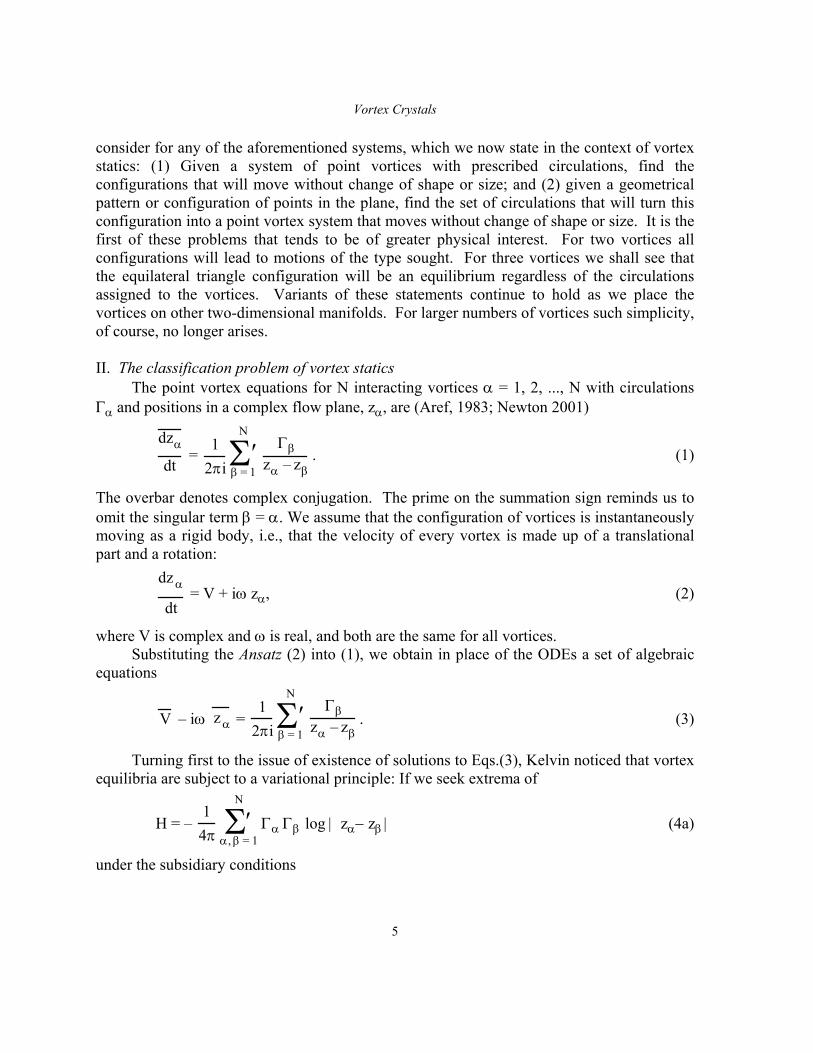
consider for any of the aforementioned systems, which we now state in the context of vortex statics: (1) Given a system of point vortices with prescribed circulations, find the configurations that will move without change of shape or size; and (2) given a geometrical pattern or configuration of points in the plane, find the set of circulations that will turn this configuration into a point vortex system that moves without change of shape or size. It is the first of these problems that tends to be of greater physical interest. For two vortices all configurations will lead to motions of the type sought. For three vortices we shall see that the equilateral triangle configuration will be an equilibrium regardless of the circulations assigned to the vortices. Variants of these statements continue to hold as we place the vortices on other two-dimensional manifolds. For larger numbers of vortices such simplicity, of course, no longer arises. II. The classification problem of vortex statics The point vortex equations for N interacting vortices α = 1, 2, ..., N with circulations Γα and positions in a complex flow plane, zα, are (Aref, 1983; Newton 2001)
dzα
dt =
12πi
Γβzα – zβ
Σ′β = 1
N
. (1)
The overbar denotes complex conjugation. The prime on the summation sign reminds us to omit the singular term β = α. We assume that the configuration of vortices is instantaneously moving as a rigid body, i.e., that the velocity of every vortex is made up of a translational part and a rotation:
dz α
dt = V + iω zα, (2)
where V is complex and ω is real, and both are the same for all vortices. Substituting the Ansatz (2) into (1), we obtain in place of the ODEs a set of algebraic equations
V – iω z α = 1
2πi
Γβzα – zβ
Σ′β = 1
N
. (3)
Turning first to the issue of existence of solutions to Eqs.(3), Kelvin noticed that vortex equilibria are subject to a variational principle: If we seek extrema of
H = – 1
4π
Γα ΓβΣ′
α, β = 1
N
log | zα− zβ | (4a)
under the subsidiary conditions
Aref, Newton, Stremler, Tokieda & Vainchtein
6
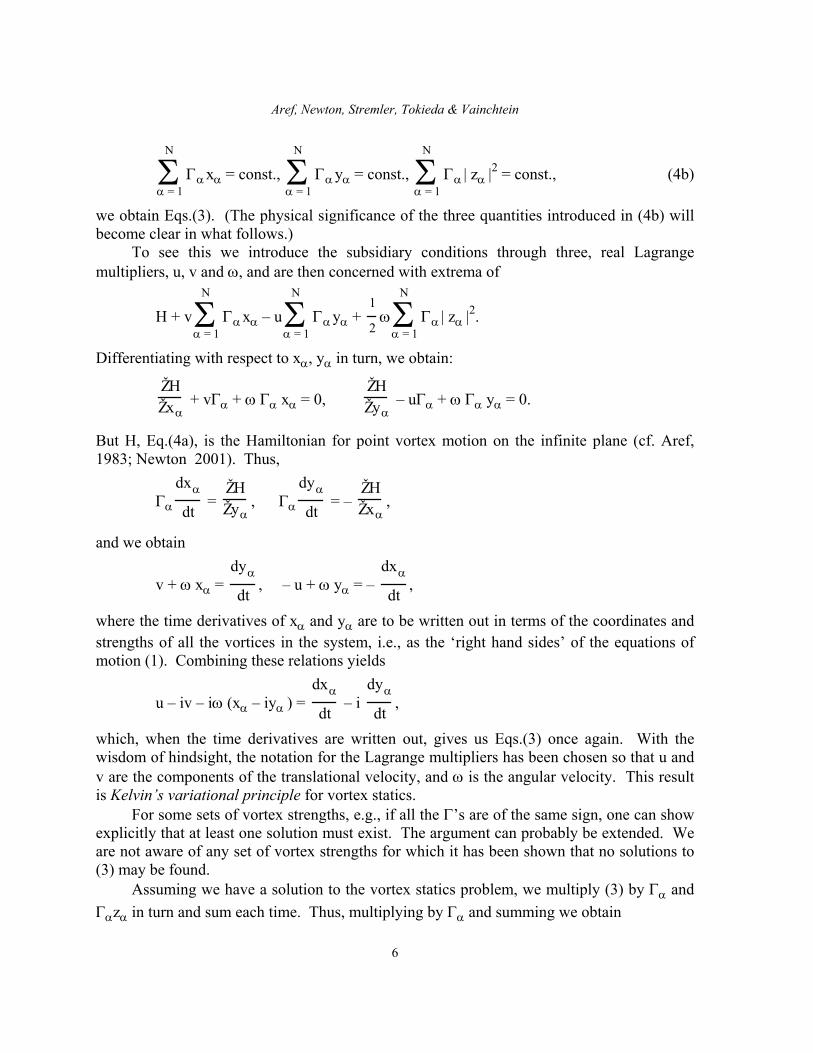
ΓαΣα = 1
N
xα = const.,
ΓαΣα = 1
N
yα = const.,
ΓαΣα = 1
N
| zα |2 = const., (4b)
we obtain Eqs.(3). (The physical significance of the three quantities introduced in (4b) will become clear in what follows.) To see this we introduce the subsidiary conditions through three, real Lagrange multipliers, u, v and ω, and are then concerned with extrema of
H + v
ΓαΣα = 1
N
xα – u
ΓαΣα = 1
N
yα + 1
2ω
ΓαΣ
α = 1
N
| zα |2.
Differentiating with respect to xα, yα in turn, we obtain:
ŽH
Žxα + vΓα + ω Γα xα = 0,
ŽHŽyα
– uΓα + ω Γα yα = 0.
But H, Eq.(4a), is the Hamiltonian for point vortex motion on the infinite plane (cf. Aref, 1983; Newton 2001). Thus,
Γα
dxα
dt =
ŽHŽyα
, Γα
dyα
dt = –
ŽHŽxα
,
and we obtain
v + ω xα = dyα
dt, – u + ω yα = –
dxα
dt,
where the time derivatives of xα and yα are to be written out in terms of the coordinates and strengths of all the vortices in the system, i.e., as the ‘right hand sides’ of the equations of motion (1). Combining these relations yields
u – iv – iω (xα – iyα ) = dxα
dt – i
dyα
dt,
which, when the time derivatives are written out, gives us Eqs.(3) once again. With the wisdom of hindsight, the notation for the Lagrange multipliers has been chosen so that u and v are the components of the translational velocity, and ω is the angular velocity. This result is Kelvin’s variational principle for vortex statics. For some sets of vortex strengths, e.g., if all the Γ’s are of the same sign, one can show explicitly that at least one solution must exist. The argument can probably be extended. We are not aware of any set of vortex strengths for which it has been shown that no solutions to (3) may be found. Assuming we have a solution to the vortex statics problem, we multiply (3) by Γα and Γαzα in turn and sum each time. Thus, multiplying by Γα and summing we obtain
Vortex Crystals
7
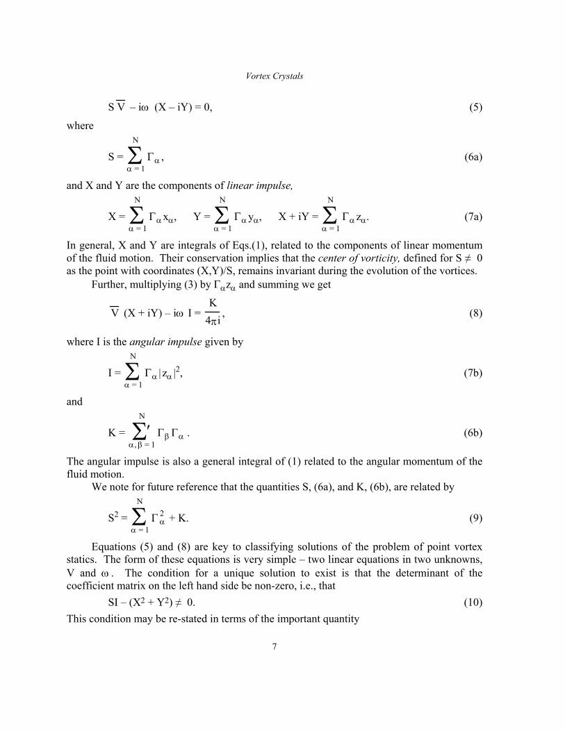
S V – iω (X – iY) = 0, (5)
where
S =
ΓαΣα = 1
N
, (6a)
and X and Y are the components of linear impulse,
X =
ΓαΣα = 1
N
xα, Y =
ΓαΣα = 1
N
yα, X + iY =
ΓαΣα = 1
N
zα. (7a)
In general, X and Y are integrals of Eqs.(1), related to the components of linear momentum of the fluid motion. Their conservation implies that the center of vorticity, defined for S ≠ 0 as the point with coordinates (X,Y)/S, remains invariant during the evolution of the vortices. Further, multiplying (3) by Γαzα and summing we get
V (X + iY) – iω I = K
4πi, (8)
where I is the angular impulse given by
I =
ΓαΣα = 1
N
| zα |2, (7b)
and
K =
Γβ ΓαΣ′α, β = 1
N
. (6b)
The angular impulse is also a general integral of (1) related to the angular momentum of the fluid motion. We note for future reference that the quantities S, (6a), and K, (6b), are related by
S2 =
Γ α2Σ
α = 1
N
+ K. (9)
Equations (5) and (8) are key to classifying solutions of the problem of point vortex statics. The form of these equations is very simple – two linear equations in two unknowns, V and ω . The condition for a unique solution to exist is that the determinant of the coefficient matrix on the left hand side be non-zero, i.e., that SI – (X2 + Y2) ≠ 0. (10) This condition may be re-stated in terms of the important quantity
Aref, Newton, Stremler, Tokieda & Vainchtein
8
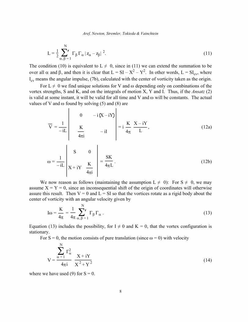
L = 12
Γβ ΓαΣ′
α, β = 1
N
| zα – zβ | 2. (11)
The condition (10) is equivalent to L ≠ 0, since in (11) we can extend the summation to be over all α and β, and then it is clear that L = SI – X2 – Y2. In other words, L = SIcv, where Icv means the angular impulse, (7b), calculated with the center of vorticity taken as the origin. For L ≠ 0 we find unique solutions for V and ω depending only on combinations of the vortex strengths, S and K, and on the integrals of motion X, Y and I. Thus, if the Ansatz (2) is valid at some instant, it will be valid for all time and V and ω will be constants. The actual values of V and ω found by solving (5) and (8) are
V = 1
– iL
0 – i X – iY
K
4πi– iI
= i K
4π
X – iYL
, (12a)
ω = 1
– iL
S 0
X + iYK
4πi
= SK
4πL. (12b)
We now reason as follows (maintaining the assumption L ≠ 0): For S ≠ 0, we may assume X = Y = 0, since an inconsequential shift of the origin of coordinates will otherwise assure this result. Then V = 0 and L = SI so that the vortices rotate as a rigid body about the center of vorticity with an angular velocity given by
Iω = K
4π =
1
4π
Γβ ΓαΣ′
α, β = 1
N
. (13)
Equation (13) includes the possibility, for I ≠ 0 and K = 0, that the vortex configuration is stationary. For S = 0, the motion consists of pure translation (since ω = 0) with velocity
V =
Γα
2Σα = 1
N
4πi
X + iY
X 2 + Y 2 (14)
where we have used (9) for S = 0.
Vortex Crystals
9
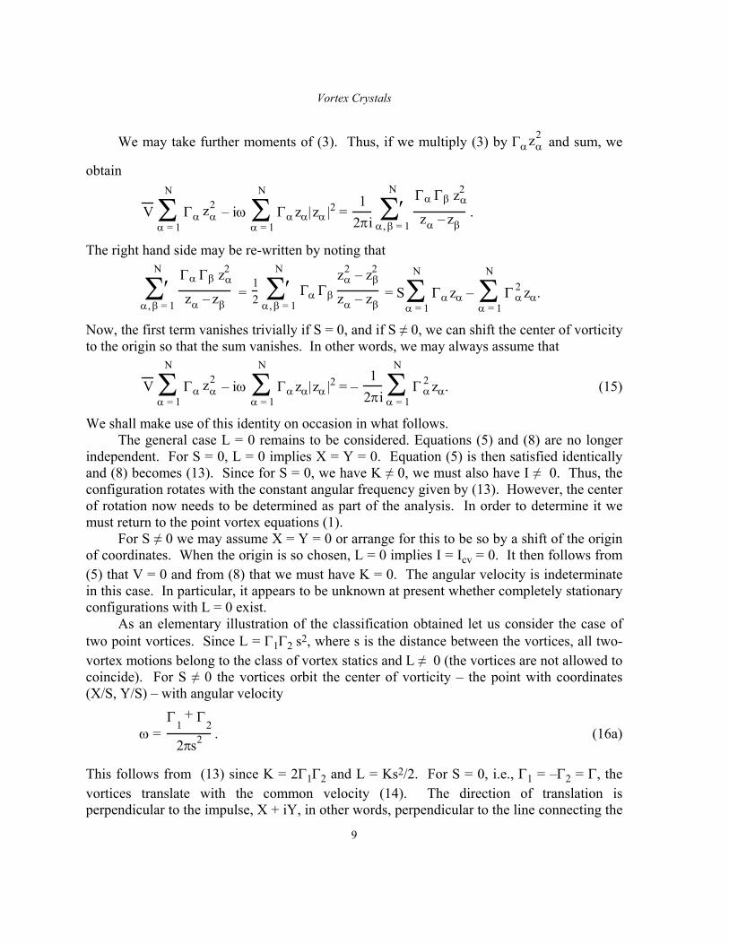
We may take further moments of (3). Thus, if we multiply (3) by Γα zα
2 and sum, we
obtain
V
ΓαΣα = 1
N
zα2 – iω
ΓαΣ
α = 1
N
zα| zα |2 = 1
2πi
Γα Γβ zα2
zα – zβΣ′
α, β = 1
N
.
The right hand side may be re-written by noting that
Γα Γβ zα
2
zα – zβΣ′
α, β = 1
N
=
12
Γα Γβ
zα2 – zβ
2
zα – zβΣ′
α, β = 1
N
= S
ΓαΣα = 1
N
zα –
Γ α2Σ
α = 1
N
zα.
Now, the first term vanishes trivially if S = 0, and if S ≠ 0, we can shift the center of vorticity to the origin so that the sum vanishes. In other words, we may always assume that
V
ΓαΣα = 1
N
zα2 – iω
ΓαΣ
α = 1
N
zα| zα |2 = – 1
2πi
Γ α
2Σα = 1
N
zα. (15)
We shall make use of this identity on occasion in what follows. The general case L = 0 remains to be considered. Equations (5) and (8) are no longer independent. For S = 0, L = 0 implies X = Y = 0. Equation (5) is then satisfied identically and (8) becomes (13). Since for S = 0, we have K ≠ 0, we must also have I ≠ 0. Thus, the configuration rotates with the constant angular frequency given by (13). However, the center of rotation now needs to be determined as part of the analysis. In order to determine it we must return to the point vortex equations (1). For S ≠ 0 we may assume X = Y = 0 or arrange for this to be so by a shift of the origin of coordinates. When the origin is so chosen, L = 0 implies I = Icv = 0. It then follows from (5) that V = 0 and from (8) that we must have K = 0. The angular velocity is indeterminate in this case. In particular, it appears to be unknown at present whether completely stationary configurations with L = 0 exist. As an elementary illustration of the classification obtained let us consider the case of two point vortices. Since L = Γ1Γ2 s2, where s is the distance between the vortices, all two-vortex motions belong to the class of vortex statics and L ≠ 0 (the vortices are not allowed to coincide). For S ≠ 0 the vortices orbit the center of vorticity – the point with coordinates (X/S, Y/S) – with angular velocity
ω = Γ1
+ Γ2
2πs2 . (16a)
This follows from (13) since K = 2Γ1Γ2 and L = Ks2/2. For S = 0, i.e., Γ1 = –Γ2 = Γ, the vortices translate with the common velocity (14). The direction of translation is perpendicular to the impulse, X + iY, in other words, perpendicular to the line connecting the
Aref, Newton, Stremler, Tokieda & Vainchtein
10
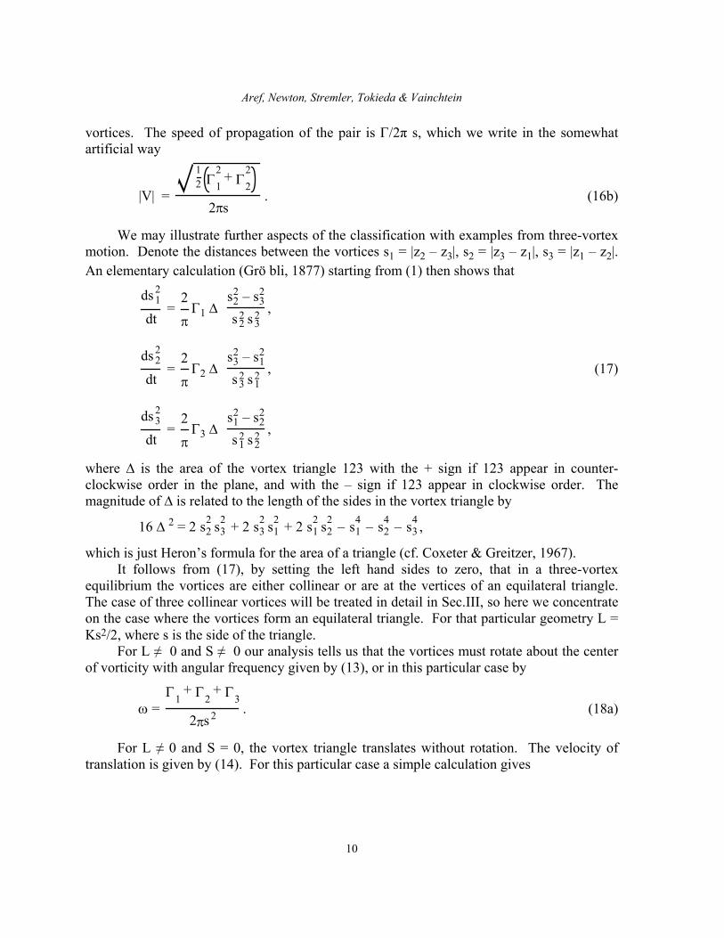
vortices. The speed of propagation of the pair is Γ/2π s, which we write in the somewhat artificial way
|V| =
12 Γ1
2 + Γ22
2πs. (16b)
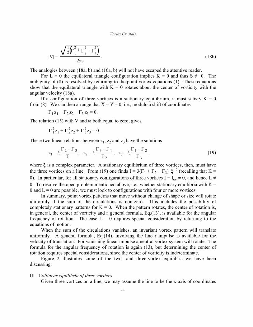
We may illustrate further aspects of the classification with examples from three-vortex motion. Denote the distances between the vortices s1 = |z2 – z3|, s2 = |z3 – z1|, s3 = |z1 – z2|. An elementary calculation (Grö bli, 1877) starting from (1) then shows that
ds 12
dt =
2
πΓ1 ∆
s22 – s3
2
s 22 s 3
2 ,
ds 22
dt =
2
πΓ2 ∆
s32 – s1
2
s 32 s 1
2 , (17)
ds 32
dt =
2
πΓ3 ∆
s12 – s2
2
s 12 s 2
2 ,
where ∆ is the area of the vortex triangle 123 with the + sign if 123 appear in counter-clockwise order in the plane, and with the – sign if 123 appear in clockwise order. The magnitude of ∆ is related to the length of the sides in the vortex triangle by
16 ∆ 2 = 2 s22 s3
2 + 2 s32 s1
2 + 2 s12 s2
2 – s14 – s2
4 – s34 ,
which is just Heron’s formula for the area of a triangle (cf. Coxeter & Greitzer, 1967). It follows from (17), by setting the left hand sides to zero, that in a three-vortex equilibrium the vortices are either collinear or are at the vertices of an equilateral triangle. The case of three collinear vortices will be treated in detail in Sec.III, so here we concentrate on the case where the vortices form an equilateral triangle. For that particular geometry L = Ks2/2, where s is the side of the triangle. For L ≠ 0 and S ≠ 0 our analysis tells us that the vortices must rotate about the center of vorticity with angular frequency given by (13), or in this particular case by
ω = Γ1+ Γ2
+ Γ3
2πs 2 . (18a)
For L ≠ 0 and S = 0, the vortex triangle translates without rotation. The velocity of translation is given by (14). For this particular case a simple calculation gives
Vortex Crystals
11
|V| =
12 Γ1
2 + Γ22 + Γ3
2
2πs. (18b)
The analogies between (18a, b) and (16a, b) will not have escaped the attentive reader. For L = 0 the equilateral triangle configuration implies K = 0 and thus S ≠ 0. The ambiguity of (8) is resolved by returning to the point vortex equations (1). These equations show that the equilateral triangle with K = 0 rotates about the center of vorticity with the angular velocity (18a). If a configuration of three vortices is a stationary equilibrium, it must satisfy K = 0 from (8). We can then arrange that X = Y = 0, i.e., modulo a shift of coordinates Γ1 z1 + Γ2 z2 + Γ3 z3 = 0.
The relation (15) with V and ω both equal to zero, gives
Γ 12 z1 + Γ 2
2 z2 + Γ 32 z3 = 0.
These two linear relations between z1, z2 and z3 have the solutions
z1 = ξ Γ 2 – Γ 3
Γ 1, z2 = ξ
Γ 3 – Γ 1
Γ 2, z3 = ξ
Γ 1 – Γ 2
Γ 3, (19)
where ξ is a complex parameter. A stationary equilibrium of three vortices, then, must have the three vortices on a line. From (19) one finds I = 3(Γ1 + Γ2 + Γ3)| ξ |2 (recalling that K = 0). In particular, for all stationary configurations of three vortices I = Icv ≠ 0, and hence L ≠ 0. To resolve the open problem mentioned above, i.e., whether stationary equilibria with K = 0 and L = 0 are possible, we must look to configurations with four or more vortices. In summary, point vortex patterns that move without change of shape or size will rotate uniformly if the sum of the circulations is non-zero. This includes the possibility of completely stationary patterns for K = 0. When the pattern rotates, the center of rotation is, in general, the center of vorticity and a general formula, Eq.(13), is available for the angular frequency of rotation. The case L = 0 requires special consideration by returning to the equations of motion. When the sum of the circulations vanishes, an invariant vortex pattern will translate uniformly. A general formula, Eq.(14), involving the linear impulse is available for the velocity of translation. For vanishing linear impulse a neutral vortex system will rotate. The formula for the angular frequency of rotation is again (13), but determining the center of rotation requires special considerations, since the center of vorticity is indeterminate. Figure 2 illustrates some of the two- and three-vortex equilibria we have been discussing. III. Collinear equilibria of three vortices Given three vortices on a line, we may assume the line to be the x-axis of coordinates
Aref, Newton, Stremler, Tokieda & Vainchtein
12
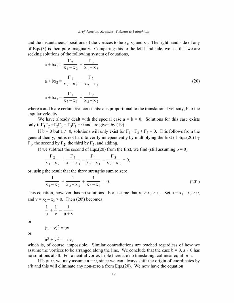
and the instantaneous positions of the vortices to be x1, x2 and x3. The right hand side of any of Eqs.(3) is then pure imaginary. Comparing this to the left hand side, we see that we are seeking solutions of the following system of equations,
a + bx1 = Γ 2
x 1 – x 2 +
Γ 3x 1 – x 3
a + bx2 = Γ 1
x 2 – x 1 +
Γ 3x 2 – x 3
(20)
a + bx3 = Γ 1
x 3 – x 1 +
Γ 2x 3 – x 2
where a and b are certain real constants: a is proportional to the translational velocity, b to the angular velocity. We have already dealt with the special case a = b = 0. Solutions for this case exists only if Γ1Γ2 +Γ2Γ3 + Γ3Γ1 = 0 and are given by (19). If b = 0 but a ≠ 0, solutions will only exist for Γ1 +Γ2 + Γ3 = 0. This follows from the general theory, but is not hard to verify independently by multiplying the first of Eqs.(20) by Γ1, the second by Γ2, the third by Γ3, and adding. If we subtract the second of Eqs.(20) from the first, we find (still assuming b = 0)
Γ 2
x 1 – x 2 +
Γ 3x 1 – x 3
– Γ 1
x 2 – x 1 –
Γ 3x 2 – x 3
= 0,
or, using the result that the three strengths sum to zero,
1
x 1 – x 2 +
1x 2 – x 3
+ 1
x 3 – x 1 = 0. (20′ )
This equation, however, has no solutions. For assume that x1 > x2 > x3. Set u = x1 – x2 > 0, and v = x2 – x3 > 0. Then (20′) becomes
1u
+ 1v
= 1
u + v
or (u + v)2 = uv or u2 + v2 = – uv, which is, of course, impossible. Similar contradictions are reached regardless of how we assume the vortices to be arranged along the line. We conclude that the case b = 0, a ≠ 0 has no solutions at all. For a neutral vortex triple there are no translating, collinear equilibria. If b ≠ 0, we may assume a = 0, since we can always shift the origin of coordinates by a/b and this will eliminate any non-zero a from Eqs.(20). We now have the equation
Vortex Crystals
13
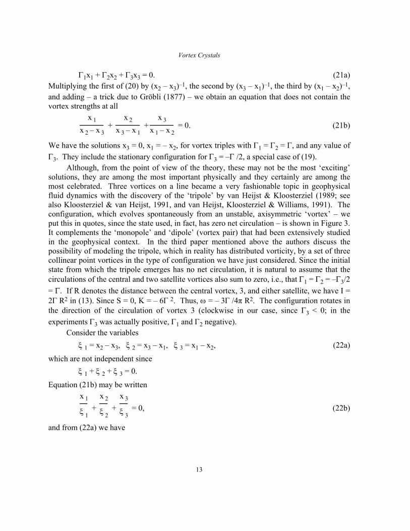
Γ1x1 + Γ2x2 + Γ3x3 = 0. (21a) Multiplying the first of (20) by (x2 – x3)–1, the second by (x3 – x1)–1, the third by (x1 – x2)–1, and adding – a trick due to Gröbli (1877) – we obtain an equation that does not contain the vortex strengths at all
x 1
x 2 – x 3 +
x 2
x 3 – x 1 +
x 3
x 1 – x 2 = 0. (21b)
We have the solutions x3 = 0, x1 = – x2, for vortex triples with Γ1 = Γ2 = Γ, and any value of Γ3. They include the stationary configuration for Γ3 = –Γ /2, a special case of (19). Although, from the point of view of the theory, these may not be the most ‘exciting’ solutions, they are among the most important physically and they certainly are among the most celebrated. Three vortices on a line became a very fashionable topic in geophysical fluid dynamics with the discovery of the ‘tripole’ by van Heijst & Kloosterziel (1989; see also Kloosterziel & van Heijst, 1991, and van Heijst, Kloosterziel & Williams, 1991). The configuration, which evolves spontaneously from an unstable, axisymmetric ‘vortex’ – we put this in quotes, since the state used, in fact, has zero net circulation – is shown in Figure 3. It complements the ‘monopole’ and ‘dipole’ (vortex pair) that had been extensively studied in the geophysical context. In the third paper mentioned above the authors discuss the possibility of modeling the tripole, which in reality has distributed vorticity, by a set of three collinear point vortices in the type of configuration we have just considered. Since the initial state from which the tripole emerges has no net circulation, it is natural to assume that the circulations of the central and two satellite vortices also sum to zero, i.e., that Γ1 = Γ2 = –Γ3/2 = Γ. If R denotes the distance between the central vortex, 3, and either satellite, we have I = 2Γ R2 in (13). Since S = 0, K = – 6Γ 2. Thus, ω = – 3Γ /4π R2. The configuration rotates in the direction of the circulation of vortex 3 (clockwise in our case, since Γ3 < 0; in the experiments Γ3 was actually positive, Γ1 and Γ2 negative).
Consider the variables ξ 1 = x2 – x3, ξ 2 = x3 – x1, ξ 3 = x1 – x2, (22a)
which are not independent since ξ 1 + ξ 2 + ξ 3 = 0.
Equation (21b) may be written
x 1
ξ 1 +
x 2
ξ 2 +
x 3
ξ 3 = 0, (22b)
and from (22a) we have
Aref, Newton, Stremler, Tokieda & Vainchtein
14
x1 = Γ 2 ξ3
– Γ 3 ξ 2
Γ 1+ Γ2
+ Γ 3
, x2 = Γ 3 ξ1
– Γ 1 ξ 3
Γ 1+ Γ2
+ Γ 3
, x3 = Γ 1 ξ2
– Γ 2 ξ 1
Γ 1+ Γ2
+ Γ 3
. (22c)
Equation (21a) is now identically satisfied, and (22b) becomes
Γ 1
ξ2
ξ3
–ξ3
ξ2
+
Γ 2
ξ3
ξ1
–ξ1
ξ3
+
Γ 3
ξ1
ξ2
–ξ2
ξ1
= 0. (23)
Choose one of the ratios between the ξ’s as a new independent variable, e.g.,
z = ξ 1
ξ 3
= x 2 – x 3
x 1 – x 2, (24)
and note that we then have
ξ 2
ξ 3
= – ξ 1
+ ξ 3
ξ 3
= – 1 – z,
ξ 1
ξ 2
= ξ 1
ξ 3
ξ 3
ξ 2
= – z
1 + z.
Thus (23) becomes
Γ1
– 1 – z +1
1 + z + Γ2
1z
– z + Γ3
–z
1 + z+ 1 +
1z
= 0,
which is a cubic equation for determining z: (Γ1 + Γ2)z3 + (2Γ1 + Γ2)z2 – (Γ2 + 2Γ3)z – (Γ2 + Γ3) = 0. (25)
A related equation appears in the paper by Borisov & Lebedev (1998). Equation (25) will always have at least one real solution, and for Γ2 + Γ3 ≠ 0 this solution will be non-zero and therefore physically acceptable according to the definition, (24), of z. For Γ2 = – Γ3 we discard the solution z = 0 and (25) reduces to the quadratic equation
(Γ1 + Γ2)z2 + (2Γ1 + Γ2)z + Γ2 = 0. (25’)
Without loss of generality we may assume Γ1 ≥ Γ2, so this equation always has two real solutions. By way of example, for Γ1 = Γ2 = –2Γ3 = Γ, Eq.(25) takes the form: 4z3 + 6z2 – 1 = 0. In this case,we have in addition to the configuration, (i) x1:x2:x3 = 1:(–1):0, found previously, the two collinear equilibria:
Vortex Crystals
15
(ii) x1 : x2 : x3 = (1 + 3 ) : (1 – 3 ) : 4,
(iii) x1 : x2 : x3 = (1 – 3 ) : (1 + 3 ) : 4. The equilibrium (i) has I ≠ 0 and so, by (13), must be stationary, since we have K = 0. The equilibria (ii) and (iii) have I = 0 and so the angular velocity of rotation must be obtained directly from the equations of motion. In the general case the number of real solutions (one or three) is determined by the discriminant of the cubic (25). No simple criterion, e.g., in terms of symmetric functions of the vortex strengths, seems available to determine when we have just one and when we have three such equilibria. IV. Identical vortices on a line There is a surprising connection between the problem of how to place N identical vortices on a line such that the configuration rotates like a rigid body and the zeros of a well known family of orthogonal polynomials. This connection was first found by Stieltjes (1885) using the analogy with interacting line charges (see Szegö , 1959, or Marden, 1949, for further details and subsequent developments). It has later been re-discovered and utilized many times, e.g., by Eshelby, Frank & Nabarro (1951) for a model of dislocation pile-up. Here we show how this result enters the N-vortex problem: Assume N identical vortices are given, and that they are placed on a line, for convenience taken as the x-axis of coordinates, such that the configuration rotates rigidly. At issue is to determine x1, ..., xN given that they obey equations of the form
λx1 = 1
x 1 – x 2 +
1x 1 – x 3
+ . . . . . + 1
x 1 – x N,
λx2 = 1
x 2 – x 1 +
1x 2 – x 3
+ . . . . . + 1
x 2 – x N, (26)
. . .
λxN = 1
x N – x 1 +
1x N – x 2
+ . . . . + 1
x N – x N – 1 ,
where, in physical units, λ = 2πω/Γ, with ω the angular frequency of rotation and Γ the common circulation of the vortices. Since λ will be positive according to the general formula (13), we can scale all the x’s by λ1/2 and it suffices to consider Eqs.(26) with λ = 1. To solve this problem we embed x1, ..., xN as the roots of a polynomial of degree N:
P(x) = (x – x1) (x – x2)... (x – xN). (27)
This polynomial satisfies an ODE of second order which is obtained as follows. The first derivative of P is
Aref, Newton, Stremler, Tokieda & Vainchtein
16
P′ = P 1
x – x αΣα = 1
N
. (28)
A second differentiation gives
P″ = P′ 1
x – x αΣα = 1
N
– P 1
x – xα2Σ
α = 1
N
=
= P
1x – xα
1x – xβ
Σα,β = 1
N
–1
x – xα2Σ
α = 1
N
= P
1x – xα
1x – xβ
Σα, β = 1α ≠ β
N
.
The summand can be re-written:
1
x – x α
1x – x β
= 1
x – xα–
1x – xβ
1x α – x β
. (29)
In the double sum we then get, according to (26) with λ = 1,
1x – xα
1x – xβ
Σα, β = 1α ≠ β
N
= 2 1
x – x α
1x α – x β
Σ′α, β = 1
N
= 2 x α
x – x αΣα = 1
N
.
Thus,
P″ = 2P x α
x – x αΣα = 1
N
= – 2NP + 2xP′ . (30)
We recognize this equation as the differential equation satisfied by the N’th Hermite polynomial HN(x). Since the Hermite polynomial is the unique polynomial solution to this second order ODE, we have established that the solutions to (26) with λ = 1 are the roots of the N’th Hermite polynomial. The result is both intriguing and disappointing. It is intriguing because it suggests a link between point vortex dynamics and other areas of applied mathematics with which the subject a priori would seem to have no connection whatsoever. Further links between vortex statics and families of polynomials that solve apparently unrelated equations will emerge later, so the ‘intrigue’ will deepen! It is disappointing because, of course, we have accomplished little in terms of finding solutions to our problem – we have simply related one set of unknown mathematical objects, viz the vortex positions along a line, to another, viz the roots of the N’th Hermite polynomial. It is a matter of taste whether one feels more information is conveyed by saying that the vortex positions satisfy (26), or that they are roots of HN. The larger question, however, is whether the idea of a generating function for the
Vortex Crystals
17
vortex positions, such as the polynomial P(x) introduced in (27), that will satisfy a relatively simple differential equation, carries further. Such generating functions have proven extremely powerful in other areas of mathematics, for example in combinatorics, and it would be very interesting if P(x) or some generalization thereof, satisfied an ODE or PDE that allowed non-trivial results to be obtained concerning vortex motion. For the present we leave these thoughts as speculations. In Secs. VIII and IX we review some results that are available in this direction. To help a bit with the disappointment, let us note that Eq.(13) with 2πω /Γ = 1 tells us that the sum of the squares of the roots of the N’th Hermite polynomial must satisfy the ‘sum rule’
x α2Σ
α = 1
N
= 12 N(N – 1). (31)
This result is known independently. Many readers are likely to know about Hermite polynomials but not know that this simple identity holds for the sum of the squares of their roots. It is, indeed, pleasing to have a proof of (31) ‘by vortex dynamics’, i.e., as a corollary of the correspondence with vortex statics. It is possible to generalize the results just obtained somewhat. For odd N = 2n + 1 there will always be a vortex at the origin, and one can consider that this vortex might have a different circulation from the other N – 1. If the central vortex has circulation pΓ, where Γ is the common value of the circulations of the remaining vortices, then the positions of the vortices are given, up to a scaling factor, by the roots of the Laguerre polynomial
L n(p – 1 /2) (x2). For p = 1 we return to the case of N identical vortices and, indeed, H2n + 1(x) is
proportional to L n(1 /2) (x2). For p = 0 we return to the case of 2n identical vortices and H2n(x)
is known to be proportional to L n(– 1/ 2) (x2).
There is a restriction (cf. Aref, 1995) to p > –1/2 for N > 3. For the three-vortex problem p can have any value and the state is always an equilibrium. For p = –1/2 we have the stationary ‘tripole’ already mentioned following Eq.(21b) and in the discussion of Eq.(25). As N increases it is known that the roots of the N’th Hermite polynomial become more and more uniformly spaced. One would expect this from the connection with vortex statics, since in the limit N → ∞ the collinear equilibria should converge to the infinite line of equally spaced vortices, a time-honored model of a vortex sheet. In the limit, one can again consider one vortex to have a different circulation, pΓ, from the rest. The vortices are then, of course, not equally spaced and one can view this as the problem of finding the equilibrium spacing of a row of vortices with an ‘inhomogeneity’. The pleasing solution is that the vortex positions are given as the zeros of the Bessel function Jp–1/2(x). It is quite remarkable that the linearized stability analysis for these configurations can
Aref, Newton, Stremler, Tokieda & Vainchtein
18
be carried out analytically to a large extent. We shall not elaborate further on this here, since a rather accessible account exists elsewhere (Aref, 1995). Many of the underlying mathematical results were obtained by Calogero and co-workers in the 1970’s (cf. Calogero, 2001, and references therein). V. Vortex polygons Perhaps the best known equilibria for identical vortices are the vortex polygons, first studied by Kelvin stimulated by Mayer’s experiments on the floating magnets mentioned earlier, and later by many others, most notably perhaps by J. J. Thomson (1883) in his Adams Prize essay. With such strong proponents as Kelvin and Thomson the analogy of vortex equilibria to atoms was a powerful, motivating force for fundamental physics. Much time and energy was spent analyzing such states. Since the polygons are stable for small numbers of vortices, they have been sought in experimental systems that approximately realize the point vortex equations, such as superfluids and electron plasmas. The basic configuration has identical vortices at the corners of a regular N-gon. This state rotates uniformly as we may see by the following considerations: We use the Ansatz zα
= R exp(i 2π α/N), α = 0, ..., N – 1. Equations (3) (with V = 0) then yield
2π R2 ω = Γ
1 – exp[2πiα /N]Σα = 1
N – 1
. (32)
To evaluate the sum we return to the ideas in Eqs.(27) and (28). Let P(z) be a polynomial of degree N in the complex variable z with distinct roots z1, ..., zN. Then P(z) = (z – z1) ... (z – zN), (33a)
P′ (z) = P(z) 1
z – zαΣα = 1
N
. (33b)
In particular, for P(z) = zN – γ N, with γ a complex number that is not an N’th root of unity, the roots are z1 = γ, z2 = γε, ... , zN = γ ε N – 1, where ε = exp(2π i/N), and so
N z N – 1 = (zN – γ N) 1
z – γ εαΣα = 1
N
.
For z = 1 this tells us that
1
1 – γ εαΣα = 1
N
= N
1 – γN ; (γ N ≠ 1). (34a)
For γ = 1, we proceed as above but with
P1(z) = (z – ε) ... (z – ε N – 1) = zN – 1
z – 1 = 1 + z + ... + zN – 1.

Vortex Crystals
19
We now have
P1′ (z) = 1 + 2z + ... + (N – 1)zN – 2.
Hence, P1(1) = N, P1′ (1) = 12N(N – 1), and (33b) becomes
1
1 – εαΣα = 1
N – 1
= 12 (N – 1), (34b)
which also arises by taking the limit γ → 1 of (34a). Combining (34b) with (32) produces
ω = Γ
4πR2(N – 1). (35)
If we place a vortex at the center of a regular N-gon, we obtain an equilibrium of N+1 identical vortices. The vortices at the corners of the N-gon rotate as before, each with a velocity augmented by the presence of the central vortex. The central vortex is stationary by symmetry. The angular velocity of rotation is from (35)
ω = Γ
4πR2 (N – 1) + Γ
2πR2 = Γ
4πR2 (N + 1). (36)
Note that this is a configuration of N+1 vortices. The vortices at the corners of a centered, regular N-gon rotate with the same angular frequency as the vortices at the corners of an open, regular (N + 2)-gon. Actually, to have an equilibrium the central vortex need not have the same circulation as the corner vortices. Thus, consider N identical vortices of circulation Γ at the corners of a regular N-gon with a vortex of circulation pΓ at the center, where p is any real number. This configuration rotates steadily with angular velocity
ω = Γ
4πR2 (N – 1 + 2p). (37)
In particular, the configuration is stationary for p = – (N – 1)/2. For N = 3, the central vortex is then simply opposite to the three vortices at the corners of the equilateral triangle. For general N, p = – (N – 1)/2 is equivalent to K = 0. It is a classical result of Thomson (1883), corrected by Havelock (1931), and later given in modified forms by Dritschel (1985) and Aref (1995), that the regular N-gon with six or fewer identical vortices is linearly stable, the heptagon is neutrally stable in linear theory, while the open N-gon with eight or more vortices is linearly unstable. Khazin (1976) considers the non-linear stability of regular vortex polygons. The linear stability of centered, regular polygons, with a central vortex of a different strength than the ones in the polygon
Aref, Newton, Stremler, Tokieda & Vainchtein
20
itself, has been studied by Morikawa & Swenson (1971), and Mertz (1976). Cabral & Schmidt (1999) prove the following result for centered regular N-gons: If the central vortex has circulation pΓ, where Γ is the common circulation of the N vortices making up a regular N-gon, then the configuration is Liapunov stable for (N2 – 8N + 8)/16 < p < (N – 1)2/4 when N is even,
(N2 – 8N + 7)/16 < p < (N – 1)2/4 when N is odd. For N < 6 these ranges include the possibility that the circulation of the central vortex is of the opposite sign to the vortices making up the polygon, i.e., p may be negative. VI. Beyond vortex polygons For N identical vortices we now have, at least, three equilibria by direct construction: the N-vortices-on-a-line (Sec.IV), the regular N-gon, and the centered, regular (N – 1)-gon (Sec.V). For this set of vortex strengths Kelvin’s variational principle guarantees existence of a stable equilibrium for each N. Since the aforementioned three families include stable equilibria only for small N, we need to explore further possibilities. If we place N1 vortices of circulation Γ1 on one regular polygon of radius R1, and N2 vortices of circulation Γ2 on a second, concentric, regular polygon of radius R2, i.e., set zα = R exp(i 2π α/N1), α = 0, ... , N1 – 1; ζβ = R eiφ exp(i 2π β/N2), β = 0, ... , N2 – 1; then Eqs.(3) (with V = 0) require
2π R12 ω =
Γ1
1 – exp[2πiα /N1]Σα = 1
N1 – 1
+ Γ
2
1 – ξ exp[2πi(β /N2 – α /N1)]Σβ = 0
N2 – 1
, (38a)
2π R22 ω =
Γ1
1 – ξ– 1
exp[2πi(α /N1 – β /N 2)]Σα = 0
N1 – 1
+ Γ
2
1 – exp[2πiβ /N2]Σβ = 1
N2 – 1
. (38b)
The phase φ describes how much one vortex polygon is turned relative to the other and ξ = (R2/R1)eiφ. The sums are done using Eqs.(34) to yield
2π R12 ω =
12(N1 – 1)Γ1 +
N2
1 – ξN2 exp[–2πiαN2 /N1]
Γ2, (39a)
2π R22 ω =
N1
1 – ξ– N1 exp[–2πiβ N1 /N 2]
Γ1 + 12(N2 – 1)Γ2. (39b)
These relations must hold for all α and β, i.e., exp[i (φ – 2π α /N1)N2] must be real for α = 0, ... , N1 – 1, and exp[i (φ + 2π β /N2)N1] must be real for β = 0, ... , N2 – 1. Thus, φ must be a multiple of π /N1 (set β = 0) and of π /N2 (set α = 0). Without loss of generality, we see from the definition of φ that we may choose it to be either 0 or π /N1. With either choice we see
Vortex Crystals
21
that both 2N1/N2 and 2N2/N1 must be integers. Since the product of these two quantities is 4, we have just three possibilities: (a) N1 = N2; (b) 2N1 = N2; (c) N1 = 2N2. However, the right hand sides in (39) must be independent of the index, α or β. This rules out (b) and (c), and we conclude that for two nested, regular polygons to form an equilibrium, they must have the same number of vertices. This is not true if we allow polygons that are not regular, e.g., there are known equilibria consisting of nested polygons of identical vortices with different numbers of vertices, but the polygons are no longer regular. For example, there is an equilibrium of 9 identical vortices consisting of an equilateral triangle nested within a hexagon, but the hexagon is not regular. For N1 = N2 = n, where the total number of vortices is even, N = 2n, we refer to the case φ = 0 as the symmetric configuration (cf. Fig.4(a) where n = 3) and φ = π /n as the staggered configuration (cf. Fig.4(c) where n = 4). The equations (39) now simplify even further:
2π R12 ω =
12 (n – 1)Γ1 +
n
1 – ρn Γ2, 2π R2
2 ω = n ρ
n
ρn
– 1Γ1 +
12 (n – 1)Γ2, (40a)
for the symmetric configuration, and
2π R12 ω =
12 (n – 1)Γ1 +
n
1 + ρn Γ2, 2π R2
2 ω = n ρ
n
ρn
+ 1Γ1 +
12 (n – 1)Γ2, (41a)
for the staggered configuration. In these equations ρ is the real parameter R2/R1. The ratio of the second equation in (40a) to the first gives
ρn + 2 – ( 2nn – 1
+ γ )ρn – (1 + 2nn – 1
γ )ρ 2 + γ = 0, (40b)
where γ = Γ2/Γ1. Similarly, the ratio of the second equation in (41a) to the first gives
ρn + 2 – ( 2nn – 1
+ γ )ρn + (1 + 2nn – 1
γ )ρ 2 – γ = 0. (41b)
For γ = 1 Eq.(41b) has the solution ρ = 1 corresponding to the regular N-gon. Analogously, for odd n Eq.(40b) has the solution ρ = –1, since the regular N-gon in this case may be thought of as a ‘symmetric’ configuration with a negative ratio of radii. Substituting ρ = e2r, we may rewrite (40b) as (n – 1) cosh[(n + 2)r] = (3n – 1) cosh[(n – 2)r], (40c) which shows that there is a unique, positive solution for ρ when n ≥ 2. Similarly, we may rewrite (41b) as (n – 1) sinh[(n + 2)r] = (3n – 1) sinh[(n – 2)r], (41c) which gives a unique, positive solution for ρ when n ≥ 4. For n = 3 there is no nested equilateral triangle solution beyond the regular hexagon. It is interesting to note that both
Aref, Newton, Stremler, Tokieda & Vainchtein
22
(40c) and (41c) lead to the same limit, ρ → 3 as n → ∞. The existence and stability of these ‘double-rings’ was discussed by Havelock (1931) in an important paper, where particular attention was paid to the staggered case for γ = –1, a circular counterpart of the Kármán vortex street. With the notation introduced above, the equation determining the ratio of ring radii in this case is (n – 1) cosh[(n + 2)r] = (n + 1) cosh[(n – 2)r]. (42) For large n, the ratio of radii, ρ, will tend to 1 as 1 + n–1. The width-to-spacing ratio of the resulting vortex street would asymptotically be (ρ – 1):π /n or 1/π or 0.32, somewhat larger than von Kármán’s ratio for the least unstable point vortex street. If we add to a double-ring of identical vortices a vortex at the center, we obtain yet another family of equilibria with a total of N = 2n + 1 vortices. With the notation above, the ratio of radii must satisfy
ρn + 2 – 3n + 1n + 1
ρn – 3n + 1n + 1
ρ 2 + 1 = 0, (43a)
for the symmetric arrangement, or
ρn + 2 – 3n + 1n + 1
ρn + 3n + 1n + 1
ρ 2 – 1 = 0, (43b)
for the staggered arrangement. Equation (43b) has the solution ρ = 1 and, for odd n, Eq.(43a) has the solution ρ = –1, corresponding to the centered, regular 2n-gon. For each n there is a unique solution to (43a) and (43b) corresponding to nested, centered, double-polygon configurations of identical vortices, both symmetric and staggered, with an odd number of vortices in total. By way of example, for n = 2, Eq.(43a) gives the solution for five vortices on a line in the form
3ρ4 – 14ρ2 + 3 = 0. (44) On the other hand, from Sec.IV we know independently that the positions of the vortices are given by the zeros of the Hermite polynomial of degree 5. This polynomial is H5(u) = 32u5 – 160u3 + 120u = 4u(8u4 – 40u2 + 30).
The squares of the roots are 0, and (5 ± 10 )/2. These satisfy (31), as they must. The ratio
of radii is given by ρ2 = (5 + 10 )/(5 – 10 ) = ( 5 + 2 )/( 5 – 2 ) = (7 + 2 10 )/3,
which is, in fact, a solution of (44). It is possible to continue ‘nesting’ polygons in this way, although a systematic investigation does not appear to have been done. A selection of possibilities is shown in Fig.4. The only comprehensive study of such states of which we are aware is the paper by Lewis & Ratiu (1996). So long as the numbers of vertices in the polygons being nested are commensurate, the algebra appears to work out, but a precise statement is lacking in the literature. We shall return to this notion of ‘commensurability’, and its apparent role in defining allowable patterns, below.
Vortex Crystals
23
Campbell & Ziff (1978, 1979) made Kelvin’s variational principle (Sec.II) the basis of a numerical algorithm to determine equilibria of N identical vortices. Their 1978 report is often referred to as the Los Alamos Catalog. This study, in turn, was stimulated by the experimental investigation of Yarmchuk, Gordon & Packard (1979) of vortex patterns in superfluid Helium. We are concerned here with the ‘classical’ superfluid 4He, not the more exotic superfluids, 3He and the Bose-Einstein condensates (BEC) that have since also been discovered to display vortex patterns. For vortices in 3He see Lounsasmaa & Thuneberg (1999). For vortices in BECs see Butts & Rokhsar, 1999, Abo-Shaer et al., 2001, and Anglin & Ketterle, 2002)1. It would take us too far afield to describe the details of the Yarmchuk, Gordon & Packard (1979) experiment and all the physics behind it. Suffice it to say that in a sample of superfluid Helium, held in a cylindrical container and rotated about its axis at a sufficiently high angular velocity, vortices will nucleate. These vortices will, predominantly, be aligned with the axis of rotation. Quantum theory restricts vortices in superfluid Helium to being lines with cores of atomic dimensions, and restricts the circulation of the vortices to be a multiple of the quantum of circulation, h/m, where h is Planck’s constant and m the mass of a Helium atom. The value of h/m is approximately 0.001 cm2/s. Usually each vortex carries just a single quantum of circulation; in other words, the vortices are identical. To excellent accuracy the dynamics of the interacting vortices is given by the ideal fluid theory that we have been pursuing and the various states we have been discussing should arise. See the monograph by Donnelly (1991) for a discussion of vortex dynamics in a superfluid. Figure 5 reproduces experimental pictures from the paper by Yarmchuk, Gordon & Packard (1979). The white spots are ‘flow visualizations’ of the vortices, a rather complex affair in a superfluid deep within a cryostat: Ions are directed towards and trapped on the vortices. They are then pulled by an electric field along the vortex, ultimately hitting a phosphorescent screen. The pictures are of the dots on this screen, and thus are much more diffuse than the actual location of the vortices. The pattern is of macroscopic dimensions, as is the frequency of rotation of the sample. Equations such as (35) or (36), or generally (13), now take on added significance. Consider (35) for a moment. On the left hand side we have an angular frequency set by the frequency of rotation of the sample. On the right we have a radius, R, and a number of vortices N, both measurable at the macroscopic level. The only unknown is Γ = h/m, the quantum of circulation, which by its nature we may think of as a microscopic quantity and certainly one that belongs to the realm of quantum physics. The experiment just described, then, becomes one of an elite class of ‘macroscopic quantum measurements’, which have yielded many of the constants of nature with unprecedented accuracy. Unfortunately, the accuracy in determining the geometry of the patterns has not so far been high enough to compete with other techniques for arriving at a value of h/m. However, this connection does provide further motivation for understanding the detailed
1) See http://cua.mit.edu/ketterle_group/Projects_2001/Vortex_lattice/GrayLattice.jpg for pictures of vortex lattices in
BECs.
Aref, Newton, Stremler, Tokieda & Vainchtein
24
geometry of rotating vortex patterns. Campbell & Ziff (1978) investigated the range 2 ≤ N ≤ 30 in considerable detail and also did some exploratory calculations for larger N. They claim to have found all linearly stable equilibria for N ≤ 30, a claim that has so far stood the test of time. Stable vortex equilibria were of interest from the start, since if the vortex patterns were to be interpreted as ‘atoms’, as Kelvin and Thomson argued, it was presumably essential that they orbit stably. Similar arguments are applied when predicting the vortex patterns likely to be seen in experiments: The inevitable small amount of dissipation will lead the vortices to form an equilibrated pattern. On the other hand, ‘noise’ from sources not included in Eqs.(1) will act to perturb any such state, so that only vortex equilibria that are stable should be expected as the persistent patterns. The patterns in Fig.5, for example, should correspond to stable N-point-vortex equilibria (as indeed they do). However, in a Hamiltonian system stable equilibria are by their nature isolated in the sense that other states with the same values of the integrals of motion cannot evolve to them. Thus, while a stable equilibrium may be the natural end result of an evolutionary process, unstable equilibria are often more important to the dynamical evolution of an N-vortex system. Indeed, unstable equilibria can appear spontaneously during the evolution of the system, and since they are equilibria, these particular configurations, or configurations close to them, will maintain themselves for a relatively long time. In the overall appearance of the system, and in any time averaging, unstable equilibria may therefore play a dominant role. One can often view the evolution of an N-vortex system as a succession of ‘visits’ to the vicinity of the unstable equilibria, where a degree of regularity both in the spatial pattern and the temporal evolution prevails. Between these ‘visits’ the motion evolves more rapidly and characteristic configurations are not in evidence. The exclusive focus on stable equilibria that has historically dominated the subject of vortex statics may, thus, be overly restrictive. As an intriguing case in point, Fig.6 shows the results of an experiment on the evolution of a magnetized electron plasma in a so-called Malmberg-Penning trap (cf. Durkin & Fajans, 2000a,b). The plasma displays point-vortex-like structures. Once again, we have to omit the details of the experiment. O’Neil (1999) provides an account for a general audience. We must also omit an assessment of how good the analogy between plasma excitations and vortices in an ideal fluid is. Under the right experimental conditions the plasma column behaves two-dimensionally in any plane perpendicular to the applied, magnetic field, which is along the column axis. The plasma evolves through the interaction of its self-electric field with the applied magnetic field. It may be shown that this evolution is governed by equations identical to the 2D Euler equation. The electron density is the counterpart of the fluid vorticity, providing enviable experimental access to this important and usually somewhat inaccessible field. A strongly magnetized electron column is the counterpart of a 2D vortex. These plasma experiments may currently be the best physical laboratory realization in existence of the point vortex equations. In the experiments shown in Fig.6 the strong vortices (the dots in the figure) are immersed in a low-level ‘background’ vortical fluid. They equilibrate by exchanging energy with this ‘background’. During the transient, which ultimately leads to the seven-vortex pattern settling into the centered, regular hexagon seen in Fig.6(c), a certain pattern, Fig.6(b),

Vortex Crystals
25
was observed to ‘linger’ for a considerable time. This pattern is very similar to one found numerically by Aref & Vainchtein (1998), Fig.10(c), by a method to be discussed below. The state in Fig.10(c) is unstable, yet it clearly plays an important role in the dynamical evolution of the system, and it is essential to understanding the experiment. The state in Fig.10(c) does not appear in the Los Alamos Catalog. Incidentally, it was found already by Glass (1997) – see Fig.1(b) of her paper – who explored equilibrium equations for various many-body systems from a different vantage point. In Fig.7 we have reproduced some of the stable states identified and catalogued by Campbell & Ziff (1978). As in the earlier studies of floating magnets and other systems, and since most of their patterns look as though the vortices are arranged on concentric rings, they chose a convenient and visually suggestive labeling scheme, assigning to each vortex pattern a set of ‘ring numbers’. The resemblance to electron ‘shells’ in pictures of atoms found in elementary chemistry and physics texts would surely have pleased Kelvin! This notion of rings has led to various conjectures about the geometry of equilibria for identical vortices. First, one might conjecture that the symmetry group of an equilibrium is always some finite set of rotations with a ‘generator’ given by the smallest angular deviation between two vortices. This is not true. Closer inspection of the computed results shows that in many cases the vortices are not arranged on exact circles at all. Only when the ring numbers are ‘commensurate’ does one find exact rings. Thus, in Fig.7(a) neither the two central vortices nor the seven outer vortices form exact rings. Rather, the symmetry of this state is that the two inner and one of the outer vortices are on a line (which is horizontal in the figure), and the remaining six vortices are pairwise symmetrically placed with respect to this line. In Fig.7(b) the two inner vortices are at equal distances from the center of vorticity. The remaining eight are organized into two rectangles not inscribed in a single circle. This state has two perpendicular reflection axes. Figure 7(c), the counterpart of Fig.5(l), again has just an axis of symmetry – it is vertical in this illustration with one of the inner and two of the outer vortices situated on it. And so on. When an axis of symmetry exists, we can rotate the entire configuration such that the complex coordinates of the vortices can be listed as n real values followed by (N – n)/2 pairs of complex conjugate positions. Of course, n must be odd for odd N, as in Fig.7(c) where N=11 and n = 3, and even for even N, as in Fig.7(f) where N = 14 and n can be taken to be 2 (vertical axis) or 4 (horizontal axis) since this configuration has two perpendicular axes of symmetry. These empirical observations suggest that the vortex positions can arise as the roots of a ‘generating polynomial’, in the sense of Eq.(27), with real coefficients. Ideally, the equation determining such a polynomial would have arisen in another branch of mathematical physics, or the polynomials for various N would obey a recursion formula, or might otherwise be ‘known’. This idea fits neatly with the appearance of the Hermite polynomials for vortices on a line (Sec.IV), and with the appearance of the Adler-Moser polynomials for stationary configurations, to be discussed in Sec.VIII. The vortex polygons, of course, may be associated with the simple polynomials zN – 1 and z(zN – 1) for the open and centered cases, respectively. Unfortunately, this appealing approach has not thus far led to the desired breakthrough in our analytical understanding of equilibria of identical vortices.
Aref, Newton, Stremler, Tokieda & Vainchtein
26
Recently, the conjecture that all equilibria have an axis of symmetry was shown to be incorrect by the discovery through numerical computation of completely asymmetric equilibria (Aref & Vainchtein, 1998). Figure 8 shows some of these states, which have been found for 8 ≤ N ≤ 14, but probably exist for all N ≥ 8. The balance between induced velocities at work in the states in Fig.8 is quite remarkable and not at all understood analytically. The numerical algorithm used to find the states in Fig.8 is quite different from algorithms based on Kelvin’s variational principle. We discuss it in the next section since it requires some preparatory considerations that are of independent interest. Figure 8 reproduces two equilibria from Aref & Vainchtein (1998) but also includes other states that were found as part of that study but, due to space limitations imposed by the journal, not published. To establish the correspondence, let AV(x) denote panel (x) of figure 1 in Aref & Vainchtein (1998). Then Fig.8(a) is a 9-vortex counterpart of AV(d) which, in fact, appears already in Fig.1(c) of Glass (1997); 8(b) is a 10-vortex counterpart of AV(e); 8(c) is AV(f) (rotated 90°); 8(d) is AV(g) which has a clear ‘family relationship’ to 8(c); 8(e) is a representative of yet another ‘family’ of asymmetric equilibria not previously published; and 8(f) is an 11-vortex counterpart of AV(h). All these equilibria are linearly unstable. In summary, as we move beyond the regular polygon equilibria for N identical vortices, both open and centered, we encounter a large number of states. Some of these, such as the nested polygons, are sufficiently regular that an analytical understanding may be established. Others, including many of the more complex stable equilibria found by Campbell & Ziff (1978), are at best understood as local minima of the ‘free energy’ in the sense of Kelvin’s variational principle. They give the general impression of having the vortices arranged on concentric circles, but unless the ‘ring numbers’ are commensurate, this is not an accurate description of these states. Their symmetry is lower than one would expect from such a characterization. The general case, and currently the only viable conjecture, appears to be that linearly stable equilibria have an axis of symmetry. Including unstable equilibria opens up a Pandora’s box of possibilities, including many states that are not ‘round’ at all. Many of these states have the axis of symmetry (Sec.VII and Fig.10) of the stable equilibria, but completely asymmetric equilibria have also been found for eight or more vortices (Fig.8). There is at present no analytical understanding of such states. VII. Morton’s equation Consider a uniformly rotating configuration of N vortices. We focus attention on particles in the flow that move as if rigidly attached to the vortex configuration, i.e., particles for which the orbit, z(t), has the form z(0) exp(iωt), where ω is the same angular frequency that enters the equation for the vortex pattern. The vortex pattern satisfies Eq.(3) with V = 0:
– iω z α = 1
2πi
Γβzα – zβ
Σ′β = 1
N
, (45a)
and we seek the points z that satisfy the equation
Vortex Crystals
27
–iω z = 1
2πi
Γ α
z – z αΣα = 1
N
. (45b)
There is no prime on this last sum, since the particle feels the velocities induced by all the vortices. Given an equilibrium, (45a), we shall refer to points that satisfy (45b) as co-rotating points relative to that configuration. We call (45b) Morton’s equation, since problems of this type seem to have been first studied systematically in the paper by W. B. Morton (1933). For identical vortices of strength Γ, arranged in a regular N-gon of radius R, Morton’s equation takes the form
2πωΓ
z =
1
z – RεαΣα = 1
N
, (46)
where ε = exp(2π i/N). Using (34a) this becomes
2πωΓ
z = N
z1
1 – (R/z) N ,
or, introducing ζ = z/R and using (35),
(N – 1)| ζ |2 = 2N
1 – ζ– N . (47)
We see from this equation that ζ–N must be real. If we write ζ = ρ eiϕ, we must then either have ϕ = 2π n/N or ϕ = (2n + 1)π /N, n = 0, 1, ..., N – 1. In the former case ζ–N = ρ–N. In the latter ζ–N = – ρ–N. Now (47) produces two equations,
(N – 1)ρ 2 = 2N
1 – ρ– N , (48a)
and
(N – 1)ρ 2 = 2N
1 + ρ– N . (48b)
For N = 3, for example, we get ρ = 0 as a solution, and two cubics ρ 3 – 3ρ – 1 = 0, and ρ 3 – 3ρ + 1 = 0, (49) with real solutions
ρ = 2 cosπ9 ; – cos
π9 – 3 sin
π9 ; – cos
π9 + 3 sin
π9 ,

Aref, Newton, Stremler, Tokieda & Vainchtein
28
and
ρ = 2 cos 2π
9 ; – cos 2π
9 – 3 sin 2π
9 ; – cos 2π
9 + 3 sin 2π
9 ,
respectively2. Only the positive solutions are physically meaningful, so we arrive at the following nine co-rotating points for the equilateral triangle with three identical vortices:
( 3 sin 2π
9 – cos 2π
9 ) eiπ /3 2 cos 2π
9 eiπ /3 – 2 cosπ9 eiπ /3
– 3 sin 2π
9 + cos 2π
9 – 2 cos 2π
9 2 cosπ9
– ( 3 sin 2π
9 – cos 2π
9 ) ei2π /3 – 2 cos 2π
9 ei2π /3 2 cosπ9 ei2π /3
Including the origin, we have 10 solution points in all for (48) with N = 3. Figure 9 depicts the rotating equilateral triangle and its co-rotating points.
Equations (48) for general N give ρ = 0 or ρ N – 2NN – 1
ρ N – 2 = ±1. The polynomial on
the left hand side vanishes at ρ = 0, is negative for small ρ, and positive for large ρ. It has a
minimum at ρ = 2 N – 2
N – 1 . The minimum value is less than –2 for N ≥ 3. There is a
unique, positive zero at ρ = 2N
N – 1 . For ρ = 2 the polynomial is larger than 2 when N ≥ 3.
For ϕ = 2π n/N, n = 0, 1, ..., N – 1, that is, the case described by Eq.(48a), there will always
be a unique solution, ρ 3, for ρ, with 2N
N – 1 < ρ 3 < 2, and N co-rotating points all with ρ =
ρ3. For ϕ = (2n + 1)π /N, n = 0, 1, ..., N – 1, we are considering Eq.(48b). There are now
two solutions, ρ1 and ρ2, 0 < ρ1 < 2 N – 2
N – 1 < ρ2 < 2N
N – 1 for ρ. (Actually, one can easily
verify that ρ 1 < 1.) We thus obtain 2N co-rotating points for a total of 3N + 1, including the origin. One might have thought by counting powers in (45b) that it should yield at most N + 1 solutions, but the complex conjugation on the left hand side throws off this count. Thus, for
2) Since (ρ 3 – 3ρ – 1)(ρ 3 – 3ρ + 1) = ρ 6 – 6ρ4 + 9ρ2 – 1 contains only even powers, the roots of the two polynomials
arise as pairs of opposites. This may not be immediately clear from the fomulae. It is, nevertheless, true that 2 cosπ9
= cos2π9
+ √3 sin 2π9
, 2 cos 2π9
= cosπ9
+ √3 sin π9
, and – cos π9
+ √3 sin π9
= cos 2π9
– √3 sin 2π9
.
Vortex Crystals
29
the N-gon of identical vortices we found 3N + 1 solutions. A count of the number of co-rotating points as a function of the vortex strengths in the ‘general case’ has apparently not been performed but should be possible using Bézout’s theorem. Calculations show that there are usually more co-rotating points than one might immediately have surmised, and certainly more than there are vortices in the configuration. Consider now the system comprised of N vortices in an equilibrium configuration and one of the co-rotating points. For simplicity let the vortices be identical. These equations are precisely what we would write down if we were to find an equilibrium configuration of N+1 ‘vortices’, where the first N are identical and the last is a ‘vortex’ of circulation zero! Now, let this last ‘ghost’ vortex acquire a tiny circulation δ Γ, where δ << 1. Then the equilibrium equations for the system of N+1 vortices are
2πωΓ
z α = 1
z α – z βΣ′β = 1
N
+ δ
zα – zN + 1, α = 1, ..., N. (50a)
2πωΓ
z N +1 = 1
zN + 1 – z αΣα = 1
N
. (50b)
In general, the positions zα, α = 1, ... , N + 1, that solve (50) will be slightly different from the position zα, α = 1, ... , N + 1, and z that solve (45). Equations (50) thus describe an algorithm in which δ is incremented step-by-step and the system is solved at each step. In this way the (N+1)’st vortex, which started ‘life’ as a co-rotating point of the N-vortex equilibrium, may gradually be ‘grown’ to the same strength, Γ, as the remaining N vortices, i.e., δ is gradually incremented from 0 to 1. There is, of course, no guarantee that a smooth, parametric evolution will result. Indeed, numerical experiments with (50) suggest that bifurcations sometimes occur and that various procedures need to be used to negotiate bifurcation points. These may be as crude as relaxing the convergence criterion on the solution and augmenting δ further until the bifurcation value has been over-stepped, and then tightening the convergence criterion once again so that a specific solution branch is selected. Computational experience suggests that the net displacement of any of the original vortices in (50), or even the co-rotating point that is being ‘grown’ into a vortex, is quite small as δ is increased from 0 to 1. Thus, given equilibrium states for N+1 vortices, one can often guess quite reliably which of these states will be produced from a given N-vortex state and its co-rotating points. Many variations on the method just outlined are possible. More than one co-rotating point can be ‘grown’ simultaneously and, if desired, different points can be ‘grown’ at different rates. Conversely, a vortex in an (N + 1)-vortex equilibrium can be decreased in strength until it becomes a zero-circulation ‘ghost’, and a co-rotating point, in an N-vortex equilibrium. The end result is that using (50) a large number of new vortex equilibria are found, many of them quite different in nature and appearance from the concentric ring solutions in the Los Alamos Catalog. These new solutions have so far all been unstable, as
Aref, Newton, Stremler, Tokieda & Vainchtein
30
one might expect from their construction. In Fig.10 we provide a sampling of symmetric equilibria that have been obtained by this method. The state in Fig.10(c) will be recognized as the ‘slow transient’ seen in the experiment of Fig.6. All of these equilibria have an axis of symmetry. The solution method based on (50) was also the one that led to the asymmetric equilibria mentioned previously (Fig.8). We should remark that although there are many co-rotating points to use in this algorithm, there are also usually symmetries that reduce the number of these points that are intrinsically different. Thus, in Fig.9, we see that by symmetry there are only four intrinsically different co-rotating points that can be used in (50). There are yet other ways of solving Eqs.(45a) for identical vortices. Consider, for
example, the following recursion in which N new vortex positions z α are obtained from the current positions zα:
zα =
1zα – zβ
Σ′β = 1
N
Σλ = 1
N1
zλ – zµΣ′µ = 1
N 2. (51)
The construct in (51) assures that
zαΣα = 1
N
= 0;
Σα = 1
N
| zα |2 =
Σα = 1
N zα
zα =
Σα = 1
N1
zα – zβΣ′β = 1
N 2
Σλ = 1
N1
zλ – zµΣ′µ = 1
N 2 = 1. (52a)
Numerical experiments show that the iteration (51) converges to a fixed point for many different initial conditions. A fixed point of the iteration will satisfy
Ω
zα =1
zα – zβΣ′β = 1
N
; Ω =
Σλ = 1
N1
zλ – zµΣ′µ = 1
N 2
. (52b)
It is not difficult to show that in this case, because of (52a), we must have Ω = N(N – 1)/2. The final state may be renormalized to produce the desired solution to (45a) for N identical vortices. Starting with randomly chosen initial positions, this algorithm yields many equilibria not easily found by methods based on Kelvin’s variational principle. The states shown in Fig.7 were produced using this method. We comment in closing that the dynamical stability of a vortex pattern and the ability of a numerical algorithm to produce it as a solution, e.g., as a fixed point of an iterative scheme, have no simple relationship, in general. Thus, the method of Campbell & Ziff
Vortex Crystals
31
(1978) did capture some dynamically unstable equilibria even though it was designed to seek out minima of the ‘free energy’ in the sense of Kelvin’s variational principle. The other methods we have highlighted capture further dynamically unstable equilibria. Thus far no method has claimed to capture all equilibria for N less than some limit. VIII. Stationary vortex patterns It may sound surprising that configurations of vortices exist where the total circulation is non-zero, yet every vortex in the pattern remains at rest. A single vortex, of course, has precisely this property. Furthermore, when K = 0, Eq.(13) tells us that the only possible equilibria are stationary patterns, and K = 0 assures us that the sum of the circulations, S, is non-zero by (9). Simple examples, such as an equilateral triangle of identical vortices with an opposite vortex at the center, and the collinear state mentioned in (19), tell us that ‘non-trivial’ stationary equilibria exist. The question, then, is how to find solutions to Eqs.(3) of this particular type. As a point of reference we may recall that an equilateral triangle configuration of three vortices with K = 0 is not stationary but rotates about its center of vorticity, so K = 0 is a necessary but not a sufficient condition for a relative equilibrium to be stationary. For general N the most elegant and far-reaching developments have been obtained for the case when all the vortices have the same absolute value of the circulation, i.e., we have N+ vortices of circulation +Γ and N– of circulation –Γ. With this ‘quantization’ of the strengths, Eq.(9) at once stipulates that if K = 0, then (N+ – N–)2 = N+ + N–.
Denote N+ – N– by n, so that N = N+ + N– = n2, and solve the two resulting, linear equations for N+ and N– together to obtain
N– = 12 n(n – 1), N+ =
12 n(n + 1), n = 1, 2, ... (53)
Thus, the number of vortices of the two circulations must be successive triangular numbers (and we have, arbitrarily, chosen the majority population to be the vortices with positive circulation). The total number of vortices is a square. The counting in (53) captures the single vortex for n = 1, which formally constitutes the smallest vortex ‘system’ with K = 0! The equilateral triangle of identical vortices with an opposite vortex at the center will turn out to be the unique solution for n = 2. In the general case we return to the ideas of Sec.IV and set P(z) = (z – z1) ... (z – zN+
); Q(z) = (z – ζ 1) ... (z – ζ N–). (54) Here z1, ... , zN+ are the complex positions of the positive vortices, and ζ 1, ... , ζ N– the positions of the negative vortices, where N– and N+ are as in (53). The equations determining these positions in this case are Eqs.(3) with zeros on the left hand sides. Thus,

Aref, Newton, Stremler, Tokieda & Vainchtein
32
1zα – zβ
Σ′β = 1
N+
=
1
zα – ζλ
Σλ = 1
N–
,
1
ζλ
– zαΣα = 1
N+
= 1
ζλ
– ζµ
Σ′µ = 1
N–
. (55)
Now calculate as in Sec.IV
P′ (z) = P(z) 1
z – zαΣα = 1
N+
, Q′ (z) = Q(z) 1
z – ζλ
Σλ = 1
N–
;
P″ (z) = P(z) 1
z – zα
1z – zβ
Σ′α, β = 1
N+
, Q″ (z) = Q(z) 1
z – ζλ
1
z – ζµ
Σ′λ, µ = 1
N–
;
P″ (z) = 2P(z) 1
z – zα
1zα – zβ
Σ′α, β = 1
N+
, Q″ (z) = 2Q(z) 1
z – ζλ
1
ζλ
– ζµ
Σ′λ, µ = 1
N–
.
At this point we use (55) to re-write P″ (z) and Q″ (z) as
P″ (z) = 2P(z) 1
z – zαΣα = 1
N+ 1
zα – ζλ
Σλ = 1
N–
,
and
Q″ (z) = 2Q(z) 1
z – ζλ
Σλ = 1
N– 1
ζλ
– zαΣα = 1
N+
.
From these relations QP″ + PQ″ =
2PQ
Σα = 1
N+ 1
zα – ζλ
Σλ = 1
N– 1z – zα
–1
z – ζλ
= 2PQ 1
z – zαΣα = 1
N+ 1
z – ζλ
Σλ = 1
N–
,
i.e., we have QP″ + PQ″ = 2P′Q′. (56) We shall call this result Tkachenko’s equation, since it was first derived by V. K. Tkachenko (1964) in his (unpublished) thesis. Assume the center of vorticity of the entire configuration is chosen as the origin of coordinates such that
Vortex Crystals
33
zαΣα = 1
N+
–
ζλΣλ = 1
N–
= 0.
Then, from (15) we have the result
zαΣα = 1
N+
+
ζλΣλ = 1
N–
= 0,
since all the vortices have the same absolute strength, and the entire configuration is stationary. Thus,
zαΣα = 1
N+
=
ζλΣλ = 1
N–
= 0. (57)
For example, for n = 2 we now have z1 + z2 + z3 = 0, ζ1 = 0,
hence P(z) = z3 + bz + a, Q(z) = z, where a, b are coefficients to be determined. Substitution in (56) gives 6z2 = 2 (3z2 + b), i.e., b = 0, and we have P(z) = z3 + a. This implies that the three positive vortices form an equilateral triangle with the negative vortex at the center as the unique solution for n = 2. To go further we note the following simple algebraic result: Let P, Q be polynomials (not identically zero) that satisfy (56), and let R be a polynomial that satisfies R′ Q – RQ′ = P2. (58) Then P and R satisfy (56). The advantage of this is, of course, that (58) is a first order differential equation for R (given P and Q), whereas (56) is a second order differential equation for P given Q. This result permits the polynomials for successive n to be found recursively, as we shall see below. The result just stated is not difficult to prove: From the relation (58) it follows that R″ Q – RQ″ = 2PP′ . Thus,
Q(R″ P RP″ ) = P(2PP′ RQ″ ) QRP″ = 2P2P′ R(P″ Q PQ″ ). Since P, Q satisfy (56), the last term can be replaced by 2RP′ Q′ , and we have Q(R″ P + RP″ ) = 2P′ (P2 + RQ′ ) = 2QR′ P′ , where (58) has been used in the last step. Dividing by Q gives the desired result.
Aref, Newton, Stremler, Tokieda & Vainchtein
34
As just mentioned, this result allows Tkachenko’s equation (56) to be solved recursively. Consider a sequence of polynomials, Pn, generated as follows:
Pn′ + 1 Pn –1 – Pn′ –1Pn + 1 = (2n + 1) Pn2, n = 1, 2, ... (59)
starting from P0 = 1, P1 = z. For n = 1 the recursion formula (59) with these starting polynomials tells us that
P2′ = 3 z2,
i.e., P2 = z3 + const., so the start of the recursive construction is in order. Assume we have constructed polynomials through Pn recursively from (59). We wish to verify that Pn + 1, constructed from (59), and Pn satisfy (56). We shall also verify that the normalization factor, 2n + 1, on the right hand side of (59) leads to the coefficient of the highest power in Pn being 1.
We first use the result (58) with Q = Pn – 1, P = 2n + 1 Pn, and R = Pn + 1. By
assumption Pn – 1 and Pn, or equivalently Q and P, satisfy Tkachenko’s equation. Since Q, P and R satisfy (58), we conclude that P and R, or equivalently Pn and Pn + 1, satisfy (56). Next, we assume that Pn – 1 and Pn both have 1 as the coefficient of their highest order terms. Denote the coefficient of the highest degree term in Pn + 1 by An + 1. If the degree of Pn is denoted dn, equating terms of highest degree in the recursion formula (59) (both matching the degree itself and considering the coefficient) tells us that dn + 1 – 1 + dn – 1 = 2dn,
An + 1 (dn + 1 – dn – 1) = 2n + 1.
The first of these relations tells us that dn + 1 – dn = dn – dn – 1 + 1, i.e., since d0 = 0, d1 = 1 that dn + 1 – dn = n + 1, or dn = n(n + 1)/2, as we would have expected from (53). The second relation then shows that An + 1 = 1. All this is quite straightforward. What is considerably less clear is that (59), viewed as a first order ODE for Pn + 1, with Pn – 1 and Pn already determined polynomials of the appropriate degrees, will again yield a polynomial! A detailed proof may be found in Adler & Moser (1978). Elements of the proof are indicated below. Let us first show the next step of the recursion. We set P1(z) = z, P2(z) = z3 + a and seek P3(z). From (57) and our other considerations we know it has the form
P3(z) = z6 + Ez4 + Dz3 + Cz2 + bz + A,
where A, b, C, D and E are coefficients to be determined. From (59) with n = 2 (6z5 + 4Ez3 + 3Dz2 + 2Cz + b)z – (z6 + Ez4 + Dz3 + Cz2 + bz + A) = 5(z3 + a)2, or 5z6 + 3Ez4 + 2Dz3 + Cz2 – A = 5z6 + 10az3 + 5a2,
Vortex Crystals
35
i.e., P3(z) = z6 + 5az3 + bz – 5a2, (60a) where b can have any value and thus is a second, free parameter. Similarly, one finds
P4(z) = z10 +15az7 + 7bz5 + cz3 – 35abz2 + 175a3z – 73 b2 + ac, (60b)
where c is a third, free parameter. In each step of the recursion we introduce a new parameter, so that given a configuration of the minority species via the polynomial, Pn, there is a one-parameter family of polynomials, Pn + 1, whose roots give the positions of the majority species. Note that the parameter b enters (60a) through a term bP1(z) and the parameter c enters (60b) through cP2(z). It is clear from (59) that, in general, Pn + 1 is only determined up to the addition of a multiple of Pn – 1. The parameter a has dimensions of ‘length’ cubed, the parameter b dimensions of length to the fifth power, the parameter c ‘length’ to the seventh power, and so on. Stationary patterns may now be displayed by simply specifying values for a, b, c, … and solving the resulting polynomials. Some particularly symmetrical examples are shown in Fig.11. Thus, Fig.11(a) shows the solution, unique up to scale, for n = 2. In Fig.11(b) we show the 3-6 configuration for a = –1, b = 0, i.e., P2(z) = z3 – 1, P3(z) = z6 – 5z3 – 5. Figure 11(c) shows the 6-10 configuration for a = 0, b = –1, c = 0, i.e., P3(z) = z(z5 – 1), P4(z) = z10 – 7z5 – 7/3. The negative vortices form a centered, regular pentagon. The positive vortices form two nested, staggered pentagons. For 21 negative and 28 positive vortices Kadtke & Campbell (1987) find the generating polynomials: z21 + 15z14 – 66z7/5 – 11/25,
z28 + 55z21 – 2211z14/5 –9438z7/25 + 1573/125. (We have rescaled the variable z in order to simplify the coefficients.) These correspond to three nested, regular heptagons of negative vortices, staggered with respect to one another, and four, staggered, regular heptagons of positive vortices, all nested as shown in Fig.11(d). From our present vantage point such diagrams are, of course, trivial to generate. The reader may compare this situation to our discussion of relative equilibria of identical vortices, where the calculation and classification of patterns was of necessity left in a rather incomplete state. The polynomials generated by (59) are known as the Adler-Moser polynomials. They arose in studies of rational solutions of the Korteweg-deVries equation and their related ‘pole decomposition’ equations (Airault, McKean & Moser, 1976). Bartman (1983) was the first to recognize the connection between that work and Tkachenko’s equation. See also Kadtke & Campbell (1987). The Adler-Moser polynomials have a remarkably simple construction: Consider the
recursion w1 = z, wn″ = wn –1 for n ≥ 2. This clearly leads to a sequence of polynomials,
Aref, Newton, Stremler, Tokieda & Vainchtein
36
w2 = 13! z3 + az + b,
w3 = 15! z5 +
13! a z3 +
12! bz2 + cz + d,
and so on, where a, b, c, d, ... are arbitrary constants (but not the same as the arbitrary constants designated by the same symbols in Eqs.(60) above). Now consider the Wronskians W1(w1) = w1,
W2(w1, w2) = w1 w2
w1′ w2′ = w1 w2′ – w1′ w2,
W3(w1, w2, w3) =
w1 w2 w3
w1′ w2′ w3′
w1″ w2″ w3″
,
and so on. (Of course, the third row of W3 can be written in terms of the entries in the first row because of the construction of the wn.) The key insight is that the n’th Adler-Moser polynomial is proportional to the n’th Wronskian in this sequence:
Pn = 1n 3n –1 5n –2 ... (2n – 1)1 × Wn(w1, w2, ... ,wn). (61)
Adler and Moser (1978) acknowledge developments by Crum (1955) a dozen years before in establishing this elegant formula. Many interesting features of these solutions undoubtedly remain to be discovered. Let us just note one that is apparently new (although the idea behind it was suggested by Khanin, 1982). Consider replacing every positive vortex in one of these stationary equilibria by an infinitesimal version of Fig.11(a). Similarly replace every negative vortex by an infinitesimal version of that same configuration with the circulations reversed (so that it has a net negative circulation). This should, once again, be an equilibrium, since at short range we have the dominant balance that prevails within Fig.11(a), and at long range we have the balance that prevailed in the original, stationary equilibrium. The counting of vortices also works out: If we had Tn –1 = n(n – 1)/2 negative and Tn = n(n + 1)/2 positive vortices before the replacements, we will have a total of
3Tn + Tn –1 = 2n2 + n = 12 2n(2n + 1) = T2n
positive and
Tn + 3Tn –1 = 2n2 – n = 12 2n(2n – 1) = T2n –1
negative vortices after the replacements. (Elegant geometrical proofs of these identities for the triangular numbers are given by Nelsen, 1993.) In terms of the generating polynomials the replacement implies that if a pair of
Vortex Crystals
37
polynomials P, Q satisfy (56), then the pair p = P3Q, q = PQ3 should also satisfy this relation. It is straightforward, albeit slightly tedious, to check this: p′ = 3QP2P′ + P3Q′ , q′ = 3PQ2Q′ + Q3P′ ,
p″ = 6P2P′ Q′ + 6QP(P′ )2 + 3QP2P″ + P3Q″ ,
q″ = 6Q2Q′ P′ + 6PQ(Q′ )2 + 3PQ2Q″ + Q3P″ . Thus, qp″ + pq″ = 12P3Q3P′ Q′ + 6P2Q2[(QP′ )2 + (PQ′ )2] + 4P3Q3(QP″ + PQ″ ). In the last term we now use (56) for P and Q to obtain qp″ + pq″ = 6P2Q2[(QP′ )2 + (PQ′ )2] + 20P3Q3P′ Q′ . This is easily seen to equal 2p′ q′ . IX. Translating vortex patterns The vortex pair – two opposite vortices translating side by side, a 2D counterpart of the circular vortex ring – has inspired attempts to construct configurations of several point vortices, with the sum of all circulations equal to zero, that translate like a rigid body. Three vortices with sum of circulations equal to zero, placed at the vertices of an equilateral triangle, produces such a translating state according to our classification from Sec.II. Let us again consider the case of vortices of the same absolute circulation. Since the total circulation must vanish, the total number of vortices, N, is even, N = 2n, and there are n vortices of either circulation. We again let z1, ... , zn designate the complex positions of the n positive vortices, and ζ 1, ... , ζ n the positions of the n negative vortices. The vortex pair, with one vortex of either sign, corresponds to n = 1. If each vortex is translating with velocity V (a complex number giving both speed and direction of propagation), Eqs.(3) determining the vortex positions become:
2πiΓ V =
1
zα – zβΣ′β = 1
n
–
1
zα – ζλ
Σλ = 1
n
, (62a)
2πiΓ V =
1
ζλ
– zαΣα = 1
n
– 1
ζλ
– ζµ
Σ′µ = 1
n
. (62b)
The quantity on the left hand side of Eqs.(62) will appear frequently, and so we introduce the abbreviation
χ = 2πiΓ V . (62c)
For this set of circulations
Aref, Newton, Stremler, Tokieda & Vainchtein
38
K = – 2nΓ 2, (see (9)), and (12) or (14) gives
χ
zαΣα = 1
n
– ζλΣλ = 1
n
= –n. (63)
Next, consider this state from the point of view of Eq.(15), which takes the form
χ
zα2Σ
α = 1
n
– ζλ2Σ
λ = 1
n
= –
zαΣα = 1
n
–
ζλΣλ = 1
n
. (64)
Eliminating χ between (63) and (64) now gives
n
zα2Σ
α = 1
n
– ζλ2Σ
λ = 1
n
=
zαΣα = 1
n
– ζλΣλ = 1
n zαΣ
α = 1
n
+ ζλΣλ = 1
n
,
or
1
nzα
2Σα = 1
n
–
1n
zαΣα = 1
n 2
= 1
nζλ
2Σλ = 1
n
–
1n
ζλΣλ = 1
n 2
. (65)
Formally, the quantities on both sides of (65) are ‘variances’ of the complex coordinates of the vortices in the two populations. The relation (65) suffices to show that Eqs.(62) have no solution for n = 2. This is somewhat surprising, since one might have thought that two pairs, placed at a great distance from one another, would translate independently with minimal mutual influence and so would approximate a translating state for n = 2. One might further have assumed that slight adjustments to this state would make it exactly satisfy (62), and that it would then be possible to move the two pairs closer and in that way generate a one-parameter family of translating states. As we shall now show, none of this ‘physical intuition’ is correct. For n = 2, Eq.(65) becomes
12 ( z 1
2 + z 22 ) –
14 (z1 + z2)2 =
12 ( ζ 1
2 + ζ 22 ) –
14 (ζ1 + ζ2)2,
or (z1 – z2)2 = (ζ1 – ζ2)2 i.e., z1 – z2 = ± (ζ1 – ζ2). (66)
From (63) we also have χ(z1 + z2 – ζ1 – ζ2) = –2. (63′ )
Equation (66) with the + sign, taken together with (63′ ), will then give
Vortex Crystals
39
χ(z1 – ζ1) = χ(z2 – ζ2) = – 1.
Now, (63a) for z1 becomes
χ = 1
z1 – z2–
1z1 – ζ1
–1
z1 – ζ2 =
1z1 – z2
+ χ – 1
z1 – ζ2,
implying z2 = ζ2, which is unacceptable. Equation (66) with the – sign runs into a similar contradiction. Thus, for n = 2 there are no solutions to Eqs.(62). For a general discussion we again introduce ‘generating polynomials’ P(z) = (z – z1) ... (z – zn
), Q(z) = (z – ζ 1) ... (z – ζ n), (67)
and calculate as before, following Eqs.(55):
P′ (z) = P(z) 1
z – zαΣα = 1
n
, Q′ (z) = Q(z) 1
z – ζλ
Σλ = 1
n
;
P″ (z) = 2P(z) 1
z – zα
1zα – zβ
Σ′α, β = 1
n
, Q″ (z) = 2Q(z) 1
z – ζλ
1
ζλ
– ζµ
Σ′λ, µ = 1
n
.
Next, use (62) to re-write P″(z) and Q″ (z) as
P″ (z) = 2P(z) 1
z – zαΣα = 1
n
χ +1
zα – ζλ
Σλ = 1
n
,
and
Q″ (z) = 2Q(z) 1
z – ζλ
Σλ = 1
n
– χ +1
ζλ
– zαΣα = 1
n
.
From these relations we get (cf. the derivation of (56)): QP″ + PQ″ = 2χ(P′ Q – PQ′ ) + 2P′ Q′ . (68) Equating coefficients of the highest order terms gives us back (63). The vortex pair corresponds to n = 1, i.e., P(z) = z – z1, Q(z) = z – ζ 1, which solves (68) if 0 = 2χ(z – ζ1 – z + z1) + 2, i.e., if χ(z1 – ζ1) = –1.
This is the result for the translation velocity of the vortex pair in another guise.
Aref, Newton, Stremler, Tokieda & Vainchtein
40
For n = 2 we have QP″ + PQ″ = 2(z – ζ1)(z – ζ 2) + 2(z – z1)(z – z2
) = 4z2 – 2(z1 + z2 + ζ1 + ζ2)z + 2(z1z2 + ζ1ζ 2), 2χ(P′ Q – PQ′ ) = 2χ[(2z – (z1 + z2))(z – ζ1)(z – ζ 2) – (z – z1)(z – z2
)(2z – (ζ1 + ζ 2))] = 2χ[(z1 + z2 – ζ1 – ζ 2)z2 – 2(z1z2 – ζ1ζ 2)z + z1z2(ζ1 + ζ 2) – ζ1ζ 2(z1 + z2)], 2P′ Q′ = 2[2z – (z1 + z2)][2z – (ζ1 + ζ 2)] = 8z2 – 4(z1 + z2 + ζ1 + ζ 2)z + 2(z1 + z2)(ζ 1 + ζ 2). Balancing coefficients of z2 returns (63′ ). The coefficients of z give 2χ(z1z2 – ζ 1ζ 2) = – (z1 + z2 + ζ1 + ζ 2). (69a)
Finally, balancing the constant terms requires 2(z1z2 + ζ 1ζ 2) = 2χ[z1z2(ζ1 + ζ 2) – ζ 1ζ 2(z1 + z2)] + 2(z1 + z2)(ζ 1 + ζ 2). (69b)
We write the square bracket on the right hand side of (69b) as
12 (z1 + z2 + ζ1 + ζ 2)(z1z2 – ζ 1ζ 2) –
12 (z1 + z2 – ζ1 – ζ 2)(z1z2 + ζ 1ζ 2),
and then use (63′ ) and (69a) to eliminate χ in (69b). This gives
2(z1z2 + ζ 1ζ 2) = –12 (z1 + z2 + ζ1 + ζ 2)2 + 2(z1z2 + ζ 1ζ 2) + 2(z1 + z2)(ζ 1 + ζ 2),
i.e., z1 + z2 = ζ1 + ζ 2,
which contradicts (63′ ). Again, we conclude that no solution exists for n = 2. For n = 3, on the other hand, we can easily give explicit solutions. For example, set P(z) = (z + c)3 – 4c3; Q(z) = (z – c)3 + 4c3. (70) Then P′(z) = 3(z + c)2, Q′ (z) = 3(z – c)2, P″(z) = 6(z + c), and Q″(z) = 6(z – c). Thus, QP″ + Q″P = 6(z2 – c2)[(z – c)2 + (z + c)2] + 24c3[(z + c) – (z – c)] = 12(z4 + 3c4), QP′ – Q′ P = 3(z2 – c2)2 [z – c – (z + c)] + 12c3 [(z + c)2 + (z – c)2] = 6c(–z4 + 6c2z2 + 3c4), 2P′ Q′ = 18(z2 – c2)2 = 18(z4 – 2c2z2 + c4), i.e., P, Q satisfy (68) if 2cχ = 1. These configurations consist of two equilateral triangles each with vortices of one sign that are mirror images of one another.
Vortex Crystals
41
Dividing by PQ Eq.(68) may be written
(log PQ )″ + [(log P
Q )′ ]2 – 2χ(log PQ )′ = –2 (logQ)″ .
Thus, if we set
ψ(z) = exp(–χz) PQ , (71)
from which follow
ψ ′ = (– χ + P′P – Q′
Q )ψ = [– χ + (log PQ )′ ] ψ,
ψ ″ = [– χ + (log PQ )′ ]2
ψ + (log PQ )″ ψ,
and we obtain ψ ″ = –2 (logQ)″ ψ + χ2ψ . (72) If we rotate our axes so that V is real, then χ2 is a negative real number, –E, and the equation may be written – ψ ″ + Uψ = Eψ , (72′) where U = –2 (logQ)″ . In other words, ψ describes an eigenstate of Schrödinger’s equation for the potential U! This potential is derived from the polynomial Q, and the wavefunction ψ is, except for the exponential prefactor, a rational function with Q in the denominator. According to Bartman (1983), the analysis of Adler & Moser (1978) shows that solutions of the desired form can only arise when Q is one of the Adler-Moser polynomials. The corresponding polynomial in the numerator is then proportional to P(z) = exp(χz) Wn+1(w1, w2, ... ,wn, exp(–χz)). (73)
We thus arrive at the intuitively surprising conclusion that only when the number of vortices of either species is a triangular number can one find configurations that translate uniformly without change in the relative positions of the vortices. It would be nice to understand this restriction independently of the full solution to the problem, as we did in (53) for the case of stationary configurations. At present such an understanding, unfortunately, appears to be lacking. Some examples of uniformly translating patterns are shown in the paper by Kadtke & Campbell (1987). X. Vortex crystals on manifolds Our knowledge of equilibrium configurations of point-vortices on general 2D surfaces is less complete than for the unbounded plane. There are compelling reasons for studying both vortex statics and dynamics in such domains. For example, vortices in a periodic strip, which may be thought of as ‘vortices on a cylinder’ in the topological sense (sometimes called a ‘flat cylinder’), is a problem that has entered the theory of shear layers and wakes for decades. Vortices in a doubly periodic parallelogram, topologically equivalent to a torus

Aref, Newton, Stremler, Tokieda & Vainchtein
42
(i.e., a ‘flat torus’), is the canonical domain for both theory and simulation of homogeneous 2D turbulence, a topic of considerable importance to geophysical fluid dynamics. Vortex dynamics on a sphere, both rotating and non-rotating, has direct applications to the flow in a planetary atmosphere on such large scales that the curvature of the planet plays a role. This problem, then, is potentially of importance to processes in the atmosphere and oceans of Earth and to the large vortices, including the Red Spot, observed in the atmosphere of Jupiter. Even though the actual vortex structures themselves are not spread over distances comparable to the planetary radius, the velocity fields they generate, and the associated global streamline patterns, are influenced by the compact nature of the sphere, as shown in Kidambi & Newton (2000). When analyzing equilibrium configurations, it is not only the long-range interactions between the vortices that determine the structure of the equilibria, but also the detailed shape of the surface. For this reason, a complete classification of equilibria with arbitrary vortex strengths on a general 2D surface seems, at the moment, a monumental task. Nonetheless, it offers a classical setting in which techniques from both geometry and dynamics play a central role. The monograph of Aranson, Belitsky & Zhuzhoma (1996) provides a general mathematical introduction to some techniques that can be used for these problems. a. Vortices on a sphere Vortices on a spherical shell seem first to have been studied by Gromeka (1885). Special cases were taken up by Bogomolov (1977, 1979). The general solution for three vortices on a sphere was first given by Kidambi and Newton (1998) a full 120 years after Gröbli’s treatment of the planar problem! Just as the planar problem is related to other pattern-forming systems, as we have seen, there are direct connections between vortices on a sphere and the large and growing literature on the ‘charge-on-a-sphere’ problem, where one considers the equilibrium configurations of N equal point charges confined to the surface of a sphere, repelled by their mutual Coulomb interactions. This is also called the ‘dual problem for stable molecules’. Interaction laws ranging from ‘soft’ logarithmic potentials (Bergersen, Boal & Palffy-Muhoray, 1994) to ‘hard’ contact forces have been studied, and lead to the so-called Tammes problem of how to optimally pack disks on the surface of a sphere. The discovery of stable carbon-60 molecules in 1985 by Curl, Kroto, and Smalley, later recognized by the Nobel Prize in Chemistry, with atoms arranged in a soccer-ball pattern on a sphere, has stimulated more abstract mathematical studies of these buckminsterfullerenes via group-theoretic methods (cf. Chung, Kostant & Sternberg, 1994). For general treatments of n-body problems on a sphere see Lim (1998) and Montaldi (2000). The question of how to uniformly distribute points on the surface of a sphere, generalizing the obvious solution of having them equally spaced around the periphery of a circle, has relevance to Monte-Carlo computational algorithms that rely on randomly sampled data points used to approximate area integrals by taking averages over these points. An introduction can be found in Saff & Kuijlaars (1997). All of these problems have their own separate literatures, yet it seems likely that many of the techniques and ideas developed in the different contexts will be more generally applicable. The equations of motion for N point vortices on a sphere of radius R are
Vortex Crystals
43
dxα
dt =
12π
Γβ
nβ× xα – xβ
xα– xβ2Σ′
β = 1
N
, (74)
where xα and xβ are vectors originating at the center of the sphere, pointing to vortices with strengths Γα and Γβ, respectively, on the surface. The unit normal vector on the spherical surface at the position of vortex γ is nγ = xγ /R, γ = 1, ..., N. Equations (74) are the natural generalization of Eqs.(1), written in Cartesian rather than complex coordinates. They reduce to (1) if we assume the unit normal to be independent of position. Since the sphere is a closed surface, the total vorticity of the flow on a sphere, that is, the integral over the surface of the sphere of the normal component of vorticity, must vanish. Equations (74) embody this constraint in the sense that the sum of the circulations explicitly shown in (74) and a uniform background vorticity, which is not directly discernible in (74) but enters through the nature of the interaction term, satisfy the constraint of vanishing total vorticity (cf. Kimura & Okamoto, 1987). Thus, if the sum of the strengths, Γα, is zero, the point vortices carry all the vorticity in the flow. If not, one has to remember the existence of a largely passive, uniform vorticity in the background. (This is, unfortunately, not the same as the background vorticity associated with uniform rotation about an axis!) Using nβ = xβ /R in the numerator, and |xα – xβ |2 = 2(R2 – xα • xβ) in the denominator, Eqs.(74) may be recast as
dxα
dt =
– 14πR
Γβ
xα× xβ
R2 – xα• xβΣ′β = 1
N
. (75)
Another interesting reformulation arises by projecting the surface of the sphere stereo-graphically onto the plane tangent to the sphere at its north pole. This is pursued by Newton (2001; § 4.5) and the result is
dzα
dt = 1 + zα
2 2
8πiR2
Γβ
zα – zβΣ′β = 1
N
–S zα
1 + zα2 . (76)
Here zα is the complex position in the tangent plane of the projection of vortex α from the sphere, and S is again the sum of the vortex strengths (6a). The first term in the square brackets is, of course, the planar interaction term from (1), so (76) may also be viewed as a planar system with a modified interaction law between the vortices. This is intriguing in view of the several related pattern-forming systems that we have mentioned previously, and the question of how ‘universal’ the vortex crystal patterns are when the law of interaction is modified. Hally (1980) gave a discussion of the modification of the equations of motion when vortices are placed on more general surfaces of revolution. See also Kimura (1999). As R → ∞ the problem of point vortices on a sphere reduces to point vortices in a plane, as considered in the previous sections. Thus, apart from the direct physical motivations for
Aref, Newton, Stremler, Tokieda & Vainchtein
44
understanding this problem, such as the dynamics of planetary atmospheres, point vortices on a sphere may also shed light on exact solutions in the plane, ‘lifting’ certain degeneracies of the planar problem for finite values of R. Such connections are only beginning to be understood at the present time. The generalization of the linear impulse integral, (7a), is still an integral of (75), i.e., these equations conserve
M =
ΓαΣα = 1
N
xα. (77)
The generalization of the angular impulse in (7b) is also conserved, but in a trivial way, since the length of each position vector is R, so that the sum becomes SR2. The algebra that led to the conservation of L, as given by (11), however, holds virtually word for word in three dimensions. Thus,
L = 12
Γβ ΓαΣ
α, β = 1
N
| xα – xβ |2 = S2R2 – M2, (78)
is obviously a constant of the motion of Eqs.(74)-(76). More significant is the analog of the Hamiltonian (4a), which for vortices on a sphere takes the form
H = – 1
4πR2
Γα ΓβΣ′
α, β = 1
N
log | xα – xβ |2. (79)
The equations determining equilibria, the counterparts of Eqs.(3), are
ω × xα = – 1
4πRΓβ
xα× xβ
R2 – xα• xβΣ′β = 1
N
(80)
for each α, where ω, the angular velocity vector common to all the vortices, is to be determined. Similarly to what we did in deriving Eq.(5), we multiply (80) by Γα and sum on α = 1, ..., N. This gives ω × M = 0. (81) Next, as in the derivation of (8), we take the cross product of (80) with Γαxα and sum on α. This gives
ΓαΣα = 1
N
xα × (ω × xα) = – 1
4πRΓαΓβ
xα× xα × xβ
R2 – xα• xβΣ′
α, β= 1
N
. (82)
The numerator in the sum on the right is xα(xα•xβ) – R2xβ. Using the symmetry of the other factors in the summand in α and β this may just as well be written xα(xα•xβ) – R2xα = xα(xα•xβ – R2). The right hand side of (82) now simplifies dramatically:
Vortex Crystals
45
1
4πR
ΓαΓβΣ
α, β = 1α ≠ β
N
xα = 1
8π
ΓαΓβΣ
α, β = 1α ≠ β
N
(nα + nβ).
For stationary equilibria we then immediately have the necessary condition
ΓαΓβΣα, β = 1
α ≠ β
N
(nα + nβ) = 0. (83)
This is a generalization of the result K = 0 in the planar case to which it reduces when all the normal vectors nα can be assumed equal. For equilibria with a finite angular frequency of rotation we can take the scalar product of (82) with ω to obtain
ΓαΣα = 1
N
(ω × xα)2 = 1
8π
ΓαΓβΣ
α, β = 1α ≠ β
N
(nα + nβ) • ω
If M is non-zero, (81) tells us that ω is along the fixed direction of M. It is convenient to take this fixed direction as the z-axis of coordinates. Then
ΓαΣα = 1
N
(ω × xα)2 = ω 2
ΓαΣα = 1
N
( xα2 + yα
2 ) = Iω 2
where the symbol I is used, literally, as in (7b) since the sum is only over the coordinates in the xy-plane. On the right hand side we substitute nα • ω = ω cosθα, where θα is the polar angle of vortex α. Finally, then,
Iω = 1
8π
ΓαΓβΣ
α, β = 1α ≠ β
N
(cosθα + cosθβ ). (84)
This is the analog of Eq.(13) for vortices on the surface of a sphere. We note that both I on the left hand side and the double sum on the right hand side of (84) are constants for an equilibrium state. The configuration moves without change of shape so the distances between vortices dαβ = |xα – xβ | are all constants. Expanding the square of this length, we see that all scalar products xα • xβ are constants, since each position vector has length R. Thus M • xα = Mzα = MR cosθα is a constant for each α. Each vortex orbits the z-axis at constant latitude.
Aref, Newton, Stremler, Tokieda & Vainchtein
46
b. Two- and three-vortex equilibria on the sphere For two vortices we obtain from (80)
ω × x1 = Γ2
4πR
x2 × x1
R2 – x1 • x2
, (85a)
ω × x2 = Γ1
4πR
x1 × x2
R2 – x1 • x2
. (85b)
A necessary and sufficient condition for a stationary equilibrium, then, is that x1 = – x2. The vortices are antipodal. They may have any strengths. In the general case ω × x1 and ω × x2, and thus x1 and x2, point in the same or in opposite directions according as Γ1 and Γ2 have opposite signs or have the same sign. Geometrically this means that vortices 1 and 2 orbit on latitude circles with the vortices on the same longitude when the strengths are of opposite sign, and with a difference of 180° in longitude when the vortex strengths are of the same sign. Figure 12(a) illustrates the general case of two vortices of opposite sign. If the sign of Γ2 were changed, that vortex would appear on the same latitude circle but at the diametrically opposite point. Figure 12(b) shows the special case of two identical vortices, and Fig.12(c) shows the special case of opposite strengths. The angular frequency of rotation is given by (84), or in this case directly from (85): Use (81) to write ω = ωM/M, then (85a) gives
ω
M Γ2 x2 × x1 = Γ2
2πR
x2 × x1
d122
,
or
ω = M
2πRd122
S2 – L/R2
2πd122 . (86)
The last form follows from (78) and makes it obvious that in the limit R → ∞ this formula reduces to that of an orbiting pair on the plane. For three vortices on a sphere Eqs.(80) become
ω × x1 = 1
2πR
Γ2 x2 × x1
d122
+Γ3 x3 × x1
d312 , (87a)
ω × x2 = 1
2πR
Γ1 x1 × x2
d122
+Γ3 x3 × x2
d232 , (87b)
Vortex Crystals
47
ω × x3 = 1
2πR
Γ1 x1 × x3
d312
+Γ2 x2 × x3
d232 . (87c)
Taking the scalar product of (87b) with x3, we see that a necessary condition for a stationary equilibrium is that ∆ = x1 × x2 • x3 vanishes. The three vortices are co-planar, i.e., in terms of the sphere they are on the same great circle. Sufficient conditions for stationary equilibria, and for equilibria in the case of vanishing M, are more complicated (cf. the discussion of collinear equilibria of three vortices in the plane in Sec.III). The known results may be found in §4.2 of Newton (2001). In the general case we write ω = ωM/M and Eqs.(87) become
Γ2
ωM
–1
2πR d122 x2 × x1 + Γ3
ωM
–1
2πR d312 x3 × x1 = 0, (88a)
Γ1
ωM
–1
2πR d122 x1 × x2 + Γ3
ωM
–1
2πR d232 x3 × x2 = 0, (88b)
Γ1
ωM
–1
2πR d312 x1 × x3 + Γ2
ωM
–1
2πR d232 x2 × x3 = 0, (88c)
from which we conclude (by taking scalar products with x1, x2, and x3) that equilibria with non-vanishing ∆ only occur if d12 = d23 = d31, i.e., if the vortices are at the vertices of an equilateral triangle (in space). In this case, regardless of the vortex strengths, the configuration is a relative equilibrium. The angular frequency of rotation, as we see immediately from (88), is
ω = M
2πRs2 , (89)
where s is the side of the equilateral triangle. For this case L = Ks2/2 so using (78) we may write
ω = K S 2 – L/R2
4πL. (89′)
In the planar limit R → ∞ the numerator becomes KS, the denominator 4πSI, and we return to Eq.(13). The ‘degenerate’ case, M = 0 requires special considerations and we again refer the reader to Newton (2001; §4.2) for what is known. For vortices on a sphere one can derive formulae similar to (17), viz
Aref, Newton, Stremler, Tokieda & Vainchtein
48
ds 12
dt = –
1
πRΓ1 ∆
s22 – s3
2
s 22 s 3
2 ,
ds 22
dt = –
1
πRΓ2 ∆
s32 – s1
2
s 32 s 1
2 , (90)
ds 32
dt = –
1
πRΓ3 ∆
s12 – s2
2
s 12 s 2
2 ,
in essence as these are derived in the planar case. In Eqs.(90) s1 = |x2 – x3|, s2 = |x3 – x1|, s3 = |x1 – x2| and, as before, ∆ = x1 × x2 • x3. We see immediately from (90) that in order for three vortices to form a relative equilibrium we must either have ∆ = 0, or have the vortices form an equilateral triangle. The analogy to the planar case is obvious. c. Multi-vortex equilibria on a sphere Equilibria with more than three vortices on the sphere are currently an active area of research. Thus, we will simply highlight what is known to date and point the motivated reader to the relevant literature. One tried-and-true method is to take known ‘classical’ configurations in the plane and look for their analogues on the sphere. The vortex polygons, simple, centered, and nested, both in the symmetrical and the staggered configurations, that we considered in Secs.V and VI have been studied on the sphere, as have vortex street configurations (Hally, 1980). Polvani & Dritschel (1993) revisit these configurations of N equal strength vortices, placing them on a sphere at a fixed latitude, and using the longitude angle 0 ≤ θ ≤ 90° as a parameter. Their main finding is that the regular polygons are ‘more unstable’ on the sphere than in the plane, with the following linear stability ranges: For N = 3: 0° ≤ θ ≤ 90°; for N = 4: 0° ≤ θ ≤ 55°; for N = 5: 0° ≤ θ ≤ 45°; for N = 6: 0°≤ θ ≤ 27°; for N = 7 there is only linear (neutral) stability at θ = 0°. Thus, at the pole, as on the plane, the heptagon gives dividing point between stable, regular N-gons and unstable ones. As the latitude increases, the critical number required to produce a neutrally stable, regular N-gon decreases. The result of Pekarsky & Marsden (1998) extends the linear stability to non-linear stability on the whole sphere for N = 3. Boatto & Cabral (2002) have recently extended the linearized stability results to the non-linear regime for general N. An approach currently being exploited is to use group-theoretic methods to generate equilibria on the sphere, restricting the vortex strengths in such a way that discrete symmetries of the equations of motion are respected. Lim, Montaldi & Roberts (2001) consider relative equilibria made up of equal strength vortices, while Laurent-Polz (2002) considers systems comprised of n vortices of strength +Γ and n of strength –Γ. In both studies, polar vortices of equal and opposite strength can (sometimes) be added (since they lie on the axis of rotation), and these, in general, do not need to be of the same strength as the
Vortex Crystals
49
other vortices in the configuration. These papers also consider the interesting problem of bifurcation of the relative equilibria as a function of H and M. Lim, Montaldi & Roberts (2001) are able to find relative equilibria made up of rings where all vortices have the same latitude, and configurations made up of two such rings at different latitudes with the vortices on one ring staggered in longitude with respect to those on the other. For stability analyses regarding these states see Laurent-Polz, Montaldi, & Roberts (2002). Laurent-Polz (2002) considers both identical and opposite strength vortices, and is able to find a separate class of equilibria, including staggered equal and opposite rings symmetrically placed across the equator (‘vortex streets’), as shown in Figure 13. In Fig.13(a) the vortices all lie on the equator, while in Fig.13(b) they are symmetrically placed on either side of the equator. Further generalizations of the polygonal and staggered planar ring configurations and their spherical analogs arise by placing identical vortices at the vertices of each of the five Platonic solids inscribed in the sphere (Tokieda, 2001; Khushalani & Newton, 2002). Thus, the tetrahedron, octahedron, cube, icosahedron and dodecahedron yield configurations with 4, 6, 8, 12 and 20 vortices, respectively. On each of these one can, furthermore, place vortices also at the vertices of the ‘dual’ polyhedron, i.e., at the points on the sphere corresponding to the midpoints of the faces of the original polyhedron. Or one can place vortices at the midpoints of the edges of the original polyhedron. All these configurations are stationary equilibria for vortices on a sphere. Perhaps more interesting is the possibility of choosing vortices with both positive and negative circulations of the same absolute magnitude to arrive at relative equilibria that rotate about M. Shown in Fig.14 are relative equilibria for each of the Platonic solids. The tetrahedron shown in Fig.14(a) is made up of a (non-equatorial) ring of three equally spaced identical vortices, with a single vortex of opposite strength placed at the north pole. It rotates about the axis shown with angular frequency 3Γ /8πR2. The cube (hexahedron) in Fig.14(b) is formed from two rings at fixed latitude symmetrically placed across the equator, each with four equally spaced vortices placed around the ring. The signs of the vortices in the northern hemisphere are opposite those in the southern hemisphere. It rotates about the axis shown with angular frequency 3√3Γ /4πR2. The octahedron, Fig.14(c), is made up of an equatorial ring of four, identical, equally spaced vortices, together with a vortex at the north pole and one at the south pole. In general, these two polar vortices could have any strength. We show the special case of opposite polar vortices whose strengths match those on the equator. The angular frequency of rotation is Γ /2πR2 (which follows readily from (84) because the latitude angles are 0 and π/2). The icosahedron, Fig.14(d), is formed from two fixed-latitude, staggered rings of five vortices each, with opposite signs on the two rings, symmetrically placed on either side of the equator, and a vortex at each of the poles. As for the octahedron, the polar vortices can have any strength. We show the special case in which the six vortices in either hemisphere have equal strengths, and the six vortices in the northern hemisphere are of opposite strength to the six in the southern hemisphere. The angular frequency of rotation then is 5(1 + √5)Γ /8πR2. Finally, the dodecahedron, Fig.14(e), is formed by placing two sets of staggered rings symmetrically about the equator. This case is somewhat more complicated in that the vortex strengths on the outer two rings and those on the inner two
Aref, Newton, Stremler, Tokieda & Vainchtein
50
rings must be related in such a way that each of the ring pairs rotates about M with the same angular frequency. This is achieved by letting Γ1 = Γ sinθ1, Γ2 = Γ sinθ2, where θ1 and θ2 are the latitudes of the two rings. The angular frequency of rotation is 9Γ /4πR2. Undoubtedly, much more complex patterns can be formed by collections of vortices on the sphere, presumably more exotic classes such as the spiral configuration shown in figure 4 of Saff & Kuijlaars (1997) and, possibly, some with no symmetries at all as generated in the plane by Aref & Vainchtein (1998). A promising numerical technique based on Monte Carlo algorithms that locates states of lowest energy, has been developed by Assad et al. (2002). d. Vortices in a periodic strip This time-honored problem includes well-known models for the shear layer and the vortex street which may be thought of, respectively, as a single vortex and a vortex pair in a periodic strip. The quickest way to derive the equations of motion for vortices in a periodic strip, which was apparently first done by Friedmann & Poloubarinova (1928)3, is to ‘periodize’ the planar theory. Thus, consider N vortices placed at z1, ..., zN in a strip of width L and with circulations Γ1, ... , ΓN. The term periodic strip means that we consider at the same time all nL-translates of these vortices for all integers n. Formally the Hamiltonian (4a) becomes
H = – 1
4π
Σ
n = –∞
+∞ Γα ΓβΣ′
α, β = 1
N
log |zα− zβ – nL|,
which diverges as it stands. However, since additive constants in the Hamiltonian may be omitted, we subtract off a constant, divergent series to produce a finite H with the same dynamics. Thus, we consider
H = – 1
4π
Σ
n = –∞
+∞ Γα ΓβΣ′
α, β = 1
N
log |zα− zβ – nL| + 1
4π
Σ
n = –∞
+∞ Γα ΓβΣ′
α, β = 1
N
log |nL|,
and rearrange the sum by pairing terms with ±n, to produce
H = – 1
4π
Γα ΓβΣ′
α, β = 1
N
log |(zα− zβ )
1 –zα – zβ
nL
2
Πn = 1
∞
| =
(91)
– 1
4π
Γα ΓβΣ′
α, β = 1
N
log |sinπL (zα− zβ )|.
The equations of motion corresponding to (1), and arising from those equations by inclusion
3) A. Friedmann is probably best known for his cosmological solutions to Einstein’s field equations of general relativity
published in two papers from 1922 and 1924.

Vortex Crystals
51
of all the periodic images, are therefore
dzα
dt = 1
2πi
Σ′β = 1
N
Γβ Φcyl(zα – zβ ), (92a)
where
Φcyl(z) = πL cot (
πL z). (92b)
One interesting feature of these equations is that as zα − zβ → i∞ (corresponding to infinite vertical separation) the velocity induced by vortex β on vortex α does not decay to zero as in the case of the infinite plane theory, but converges to Γβ /2L. This is obvious upon calculating the circulation around a tall box of width L enclosing the point zβ. Another way to interpret this feature is to note that the limit of infinite vertical separation is, up to rescaling, equivalent to the narrowing of the period L to 0; this limit produces a continuous vortex sheet, which induces a velocity field constant everywhere above the sheet (with the opposite constant below the sheet) independently of the distance to the sheet. This is a general result of two-dimensional potential theory, possibly more familiar in the case of electrostatics, where the electrostatic force induced by a homogeneous charge distribution on an infinite line is independent of the distance to the line. The quantities X and Y in (7) are still integrals (Birkhoff & Fisher, 1959), but rigorously speaking there is a subtlety involved. Indeed, each xα in X being defined only modulo L (i.e., on the manifold a vortex that ‘leaves’ the strip at x = L, ‘reappears’ at x = 0), X is not well-defined as a function on the whole periodic strip (physically, one would have to keep track of how many times each vortex went through the strip – the instantaneous position of the vortices, of course, gives no hint of this). Nor is it much use treating X as a multi-valued function, for in general the strengths will not be rationally dependent and so the set of values L∑α Γαnα giving the ‘ambiguity’ in X will be dense in the real numbers. Nevertheless, X is well defined locally, i.e., so long as the vortices remain within the strip, and this suffices for our purposes. First integrals that are only locally defined are apt to arise when the surface on which we develop the vortex theory has non-zero first homology (or, in mathematical jargon, when the symplectic action of the symmetry group is not Hamiltonian). Such is the case with a periodic strip (topologically a cylinder) and a periodic parallelogram (topologically a torus), or any surface of genus > 0. The sphere, being simply connected, involves no such subtlety. This issue is similar to the familiar one in ideal hydrodynamics of having to introduce ‘barriers’ to define the potential for multiply connected domains. There is a partial classification result for equilibria in a periodic strip and a periodic parallelogram (Montaldi, Soulière & Tokieda, 2002). We shall describe the results for a periodic strip first. Unlike the plane, a periodic strip (cylinder) does not have rotational symmetry. It is not difficult to see that rotating equilibria are impossible. Thus, the only possibility for equilibria

Aref, Newton, Stremler, Tokieda & Vainchtein
52
is that the entire configuration translates without change of relative positions of the vortices, i.e., in (92a) all the left hand sides equal the same complex number. Multiplying (92a) by Γα and summing, and using the antisymmetry of the summand, produces the result SV= 0, where S is the sum of circulations, and V is the common velocity of translation. Equilibria of vortices in a periodic strip, then, requires either that S = 0 or, if S ≠ 0, that the equilibrium is stationary. For two vortices in a periodic strip with S = 0 the equations of motion and Φcyl being an odd function guarantees that the vortices will translate uniformly regardless of their initial separation. These configurations are the vortex streets studied by von Kármán (1911, 1912) in the cases where the direction of propagation is along the horizontal axis, and by Dolaptschiew and Maue (cf. Maue, 1940) in the general case. According to (92a) the complex velocity is given by
V = u – iv = 1
2Li cot [πL (z1 – z2)], (93)
i.e., the direction of propagation is given by v:u = – sin[πL (x1 – x2)]:sinh[
πL (y1 – y2)]. This
direction is not, in general, perpendicular to the line segment connecting the vortices, although in the ‘deperiodizing limit’, L → ∞, it converges to that direction. A stationary pair with S = 0 requires y1 = y2 and x1 – x2 = ±L/2, i.e., the vortices are uniformly spaced along the x-axis, the cylinder counterpart of the state illustrated in Fig.13(a) for vortices on a sphere. Stationary pairs with S ≠ 0 are also covered by this analysis. The uniformly spaced vortices need not have the same absolute magnitude. For three vortices with S ≠ 0 the conditions for a stationary equilibrium require
c1
Γ1
= c2
Γ2
= c3
Γ3
(94)
(Stremler, 2002). Here we have used the abbreviations
c1 = cot [ π
L (z2 – z3)], c2 = cot [πL (z3 – z1)], c3 = cot [
πL (z1 – z2)]. (95)
Cases of two vortices having opposite circulations, such as Γ1 = –Γ3, need to be considered separately. If Γ1 = –Γ3, we must have c1 = – c3 or
cot [ π
L (z2 – z3)] = – cot [πL (z1 – z2)],
sin [ π
L (z1 – z2)] cos [ π
L (z2 – z3)] + cos [πL (z1 – z2)] sin [
πL (z2 – z3)] = 0,
Vortex Crystals
53
sin [ π
L (z1 – z3)] = 0 or z1 – z3 = nL, n an integer.
But this means that vortex 1 coincides with vortex 3, or with one of its periodic images, which is unacceptable. The other cases of opposite vortices lead to similar contradictions. Hence, we conclude that when two vortices are opposite, there are no three-vortex equilibria. Except for these special cases we may use that c1, c2 and c3 are related by the addition formula for the cotangent, viz
c1 = cot [ π
L (z2 – z1 – (z3 – z1))] = 1 – c2 c3
c2 + c3,
i.e., by c1c2 + c2c3 + c3c1 = 1. (96)
If the common value of c1/Γ1, c2/Γ2 and c3/Γ3, cf. (94), is denoted ξ, (96) states that K ξ2 = 2, where K was given by (6b). To have a solution we must require K ≠ 0 and then
c1 = ±Γ1/ K /2 , c2 = ±Γ2/ K /2 , c3 = ±Γ3/ K /2 , (97)
where the same sign must be used for each of c1, c2 and c3. The nature of the resulting equilibria depends on the sign of K. For K > 0 the quantities c1, c2 and c3 are all real and the vortex separations z2 – z3, z3 – z1 and z1 – z2 must also all be real. In other words we must have y1 = y2 = y3. The vortices are on a line parallel to the x-axis. Solutions are given by
1
Γ1 cot [
πL (x2 – x3)] =
1Γ2
cot [πL (x3 – x1)] =
1Γ3
cot [πL (x1 – x2)] = ±1/ K /2 .
For example, let vortices 1 and 2 both have strength Γ and place them a distance x1 – x2 = a apart on a horizontal line. They are immobilized if we add halfway between them a vortex of strength
Γ3 = – Γ cot πa
L /cot πa
2L = Γ 1
2sec2 πa
2L– 1 .
In the deperiodizing limit, L→ ∞, this converges to –Γ /2 as it should from the unbounded plane results (cf. Sec.III). On the other hand, Γ3 vanishes when a = L/2: the two vortices are antipodal on the periodic strip and are already stationary by themselves. As a → L, the two vortices nearly meet ‘in the back’ and it takes a stronger and stronger vortex at their midpoint to prevent them from moving. For K < 0 the quantities c1, c2 and c3 in (97) are all pure imaginary. Thus, we must have
Aref, Newton, Stremler, Tokieda & Vainchtein
54
sin [ 2π
L (x1 – x2)] = sin [ 2π
L (x2 – x3)] = sin [ 2π
L (x3 – x1)] = 0,
which implies that the vortices must be on lines parallel to the y-axis offset by a multiple of L/2. If the vortices are on a vertical line, x1 = x2 = x3, we have the solutions
1
Γ1coth [
πL (y2 – y3)] =
1Γ2
coth [πL (y3 – y1)] =
1Γ3
coth [πL (y1 –
y2)] = ±1/ K /2 .
For further discussion see Stremler (2002). By way of example, let vortices 1 and 2 both have strength Γ but place them a distance y1 – y2 = b apart on the same vertical line. They are immobilized if we add at their midpoint a vortex of strength
Γ3 = – Γ coth πb
L /coth πb
2L = Γ 1
2sech2 πb
2L– 1 .
In the ‘deperiodizing limit’, L→ ∞, this again converges to –Γ /2. On the other hand, in the ‘vortex sheet limit’, b→ ∞, this converges to –Γ, also as it should. Aref & Stremler (1996) have shown how to obtain the general solution of the integrable dynamical problem of three vortices with S = 0 in a periodic strip. The approach consists in ‘mapping’ the original three-vortex problem, with vortices at locations z1, z2 and z3 of circulations Γ1, Γ2 and Γ3, respectively, in a strip of width L, onto a simpler problem, viz the problem of advection of a fictitious, passive particle in a field of certain fixed vortices derived from the strengths and first integrals X and Y of the original problem. The details of this construction are as follows: The ‘mapped’ particle is situated at z1 – z2 and moves in the field of three rows of vortices of strengths 1/Γ1, 1/Γ2 and 1/Γ3, respectively. The vortices of the first ‘family’, all of strength 1/Γ3, are located at nL, where n runs through the integers, i.e., their spacing is that of the original strip width. The vortices of the second ‘family’, all of strength 1/Γ2, are located at – (X + iY)/Γ2 + nLΓ3/Γ2, n = 0, ±1, ±2, ... The vortices of the third ‘family’, all of strength 1/Γ1, are located at (X + iY)/Γ1 + nLΓ3/Γ1, n = 0, ±1, ±2, … If the ratio of any two of Γ1, Γ2 and Γ3 is rational, then all such ratios are rational since Γ1 + Γ2 + Γ3 = 0, and the three rows repeat with a period that is a multiple of the original strip width L. Note that although the circulations of the three original vortices sum to zero, the net circulation of the advecting system is non-zero. The problem of advection of the fictitious particle is readily solved, by constructing the steady streamline pattern for the three vortex rows. Vortex equilibria correspond to stagnation points in the derived, advecting flow. These must all be saddle points. The advecting vortices themselves are the only elliptic points and correspond to two of the original vortices 1, 2, 3 coinciding. That is, all the equilibria are unstable. Several are obtained. Remarkably, they can all be calculated
Vortex Crystals
55
explicitly, as we show below. The ‘generic’ number of equilibria can be counted by topological considerations. Figure 15 shows an example of the derived streamline pattern for the case of three vortices of relative strengths 2:1:(–3). In this case the derived advection problem ‘lives’ in a periodic strip of width 3L. The solid dots are the advecting vortices. The equilibria correspond to the several saddle points seen in the pattern of separatrix streamlines. We may find these points explicitly by considerations similar to those for the stationary equilibria given previously. Thus, from the equations of motion (92) we find (Stremler, 2002):
2Li V = Γ2 c3 – Γ3 c2,
2Li V = Γ3 c1 – Γ1 c3, (98)
2Li V = Γ1 c2 – Γ2 c1.
Taking the difference of any two of these, and using S = 0, gives c1 + c2 + c3 = 0, (99)
which is the analog of (20′ ). Conversely, (99) and S = 0 assure that the right hand sides of (98) are all equal. We can now solve (96) and (99) for two of the c’s given a value of the third. For example, choosing the position of vortex 2 relative to vortex 1 gives c3, and then c1 and c2 are the two roots of the polynomial
(c – c1)(c – c2) = c2 – (c1 + c2)c + c1c2 = c2 + c3c + 1 + c32 ,
i.e.,
c1 = 12 (– c3 + i 4 + 3c3
2 ); c2 = 12 (– c3 + i 4 + 3c3
2 ),
where the signs are to be chosen such that c1 ≠ c2. Thus, for any allowable value of c3, that is for any value of c3 for which the vortices and their periodic images are all distinct, we can determine c1 and c2 such that we have a translating equilibrium. What is quite remarkable is that these configurations are independent of the values of the vortex strengths! We can populate the three points with vortices of any circulations, subject to the constraint that S = 0, and we arrive at a relative equilibrium. We have seen something of this sort before: For the equilateral triangle on the infinite plane we could place any three vortices at the vertices and always have an equilibrium. If the sum of the strengths were zero, the triangle would translate uniformly. The solutions just mentioned give rise to a large family of translating ‘vortex streets’ with three vortices, whose strengths sum to zero, per period. But there is more. As observed by Aref & Stremler (2002), the three vortex rows in the mapping construction that we have described are themselves multi-vortex equilibria with
Aref, Newton, Stremler, Tokieda & Vainchtein
56
total non-zero circulation (and, thus, stationary patterns)! This follows from the construction: Any advecting vortex corresponds via the mapping to the coincidence of one of the original vortices with another or with any one of its periodic images (based on the original strip of width L). But if two of the original vortices coincide, the three-vortex problem reduces to a two-vortex problem, the solution of which is simply that the two vortices translate in parallel. This implies that the difference z1 – z2 is constant. In other words, the rate of change of z1 – z2 vanishes at any advecting vortex. But this rate of change is just the velocity at the position of the advecting vortex (and by extension at all its periodic images). Hence, each advecting vortex finds itself at a point of vanishing advection velocity due to all the other vortices. When z1 – z2 coincides with an advecting vortex of one of the three aforementioned ‘families’, it follows that z2 – z3 and z3 – z1 coincide with advecting vortices of the other two ‘families’. The upshot is that all the advecting vortices form a stationary pattern, which then has the simple parametrization already given (restated more ‘generically’ below). This can, of course, also be verified by direct calculation using Eqs.(92). There is a three-parameter family of stationary equilibria consisting of three vortex rows. The three parameters are X, Y, and a ratio of two of the original vortex strengths Γ1, Γ2 and Γ3. In other words, take three real numbers, Γ1, Γ2 and Γ3, that sum to zero. For general complex Z place vortices of strength 1/Γ3 at nL, n integer; vortices of strength 1/Γ2 at (–Z + nL)Γ3/Γ2; vortices of strength 1/Γ1 at (Z + nL)Γ3/Γ1. (The only constraint on Z is that vortices of the three different families not coincide.) The states just given are stationary equilibria. If the ratios of Γ1, Γ2 and Γ3 are rational, the pattern repeats after some multiple of L. If these ratios are irrational, we obtain the possibility of stationary vortex patterns without long-range periodicity. With a bit of poetic license we call such patterns vortex quasi-crystals. It is presently unknown whether such states can be realized experimentally. For even N > 3, say N = 2k, and S = 0, the vortex street equilibria found for two vortices per strip can, of course, be recovered ‘in a wider strip’. The system with k = 2, two positive and two negative vortices all of the same absolute circulation, was studied by Domm (1956) in a seminal paper on the stability of vortex streets. No other families of equilibria appear to be known for N > 3. In summary, we have obtained several families of vortex equilibria, both stationary and translating, for N = 3 vortices in a periodic strip. For N > 3 we found an explicit construction of a large family of stationary equilibria with S ≠ 0. e. Vortices in a periodic parallelogram Proceeding to a periodic parallelogram we use the notation of the theory of elliptic functions for the sides, denoting them by 2ω1 and 2ω2, respectively, where τ = ω2/ω1, has positive imaginary part. Periodic squares have been used extensively for numerical simulations of homogeneous 2D turbulence. Such simulations reveal the flow to be dominated by strong discrete vortices. Hence, it is of considerable interest to study the

Vortex Crystals
57
problem of interacting vortices in this geometry. In these applications the periodic nature of the flow requires the vanishing of the total circulation for all vortices in the basic periodic parallelogram. It is also of interest to consider the problem of infinite, regular lattices of vortices since such structures arise in superfluids and, approximately, in superconductors. For the simplest case of one vortex per cell (identical vortices) Tkachenko (1966a) showed that all lattices give configurations that rotate uniformly. The angular frequency of rotation, Ω, depends on the shape of the basic cell (parallelogram), i.e., on the parameter τ. The simplest way to establish this dependence is to think of a large section of the lattice as a ‘discretized’ patch of fluid with uniform vorticity ω. Thus, on one hand, from the general relation between uniform vorticity and angular velocity we would have ω = 2Ω. On the other hand, the total circulation of the flow around the patch, which by Stokes’ theorem is ωA (with A the area of the patch) also equals NΓ, where N is the number of vortices in the patch, all of which have the common circulation Γ. That is, Ω = nΓ /2, where n is the area density of vortices. If the area of the basic cell of the lattice, i.e., the area of the periodic parallelogram, is denoted ∆ , we have Ω = Γ/2∆ . Tkachenko (1966b) also examined the stability of the various simple lattices and concluded that for small perturbations (i.e., in a linearized stability analysis) the triangular lattice is the only stable one. The Hamiltonian of the vortex motion is found to be
H = – 1
4π
Γα ΓβΣ′
α, β = 1
N
ΓαΓβ [log |ϑ1(zα− zβ |τ)| – π Im (zα – zβ) 2
∆ ], (100)
where ϑ1 is the first Jacobian theta function and ∆ = 2i ω1ω2– ω2ω1 = 4 |ω1|2 Imτ is the
area of the parallelogram (O’Neil, 1989; Stremler & Aref, 1999; Tokieda, 2001). The counterparts of Eqs.(1) or (92) are
dzα
dt = 1
2πi
Σ′β = 1
N
Γβ Φtorus(zα – zβ ), (101a)
where
Φtorus(z) = ζ (z) + πω1
∆ω1
–η 1
ω1
z – π
∆z , (101b)
where the Weierstrass ζ-function has half-periods ω1 and ω2, and η1 = ζ(ω1). The two-vortex problem with two vortices of opposite circulation again leads to uniform translation for all initial conditions. For three vortices (with the sum of the circulations equal to zero) a complete solution was provided by Stremler & Aref (1999). It follows the analysis for the periodic strip (cylinder) closely. One has to verify that the ‘mapping’ idea will work once again, which is more complicated since the induced velocities
Aref, Newton, Stremler, Tokieda & Vainchtein
58
are given by the Weierstrass ζ-function rather than by cotangents, but the end results are very similar. One finds, once again, that the dynamics of the three interacting vortices can be ‘mapped’ onto an advection problem for a fictitious particle at z1 – z2 which moves in the field of three lattices of vortices of strengths 1/Γ1, 1/Γ2 and 1/Γ3, respectively. The vortices of the first ‘family’, all of strength 1/Γ3, are located at Ωmn = 2mω1 + 2nω2, where m and n are integers, i.e., on a lattice with the same periods as the original problem. The vortices of the second ‘family’, all of strength 1/Γ2, are located at – (X + iY)/Γ2 + ΩmnΓ3/Γ2. The vortices of the third ‘family’, all of strength 1/Γ1, are located at (X + iY)/Γ1 + ΩmnΓ3/Γ1. If the strength ratios are rational, the three lattices repeat with periods that are a multiple of the original 2ω1 by 2ω2 parallelogram. In this case the sum of the circulations of the advecting vortices situated within the extended parallelogram is, indeed, zero as it must be for a periodic flow. Figure 16 shows advecting vortices and dividing streamlines for the case Γ1:Γ2:Γ3 = 2:1:(–3). Each saddle point in this figure gives a value of z1 – z2 that corresponds to an equilibrium of the three-vortex problem in the original periodic parallelogram (a square of side L in this case). If z1 – z2 is known, then given the vortex strengths, and values of X and Y, the three vortex positions are known up to translation. Furthermore, as in the case of the strip and by virtually the same argument, the three interwoven lattices of advecting vortices form a stationary equilibrium (Aref & Stremler, 2001, 2002). For rational vortex ratios these are again periodic patterns. For irrational ratios they form 2D quasi-crystals. These seem to be the only known exact results for two-dimensional vortex patterns. f. Vortices on the hyperbolic plane Apart from the study by Kimura (1999) this topic is still largely unexplored. After developing the theory of point of vortices on the plane, on a sphere, in a periodic strip, and in a periodic parallelogram, it is natural to try to do as much on other surfaces, in particular on Riemann surfaces of genus > 1. Chief interest in the hyperbolic plane stems from the fact that every orientable surface of genus > 1 is a discrete quotient of the hyperbolic plane. Here we confine ourselves to deriving the Hamiltonian for point vortices on the hyperbolic plane and mentioning a class of equilibria. Place a vortex of unit circulation at a point, and draw a circle of radius r (measured, of course, in the hyperbolic metric) around that point. This circle has length 2π sinhr (compare 2π sinr in the spherical case). The Hamiltonian H contributed by the vortex should be rotationally symmetric, so that H is a function of r alone. The circulation of the induced velocity field around the circle is
– ∂H∂r 2π sinhr = 1,
which upon integration yields
H = – 1
2πlog|tanh(r/2)|.
Vortex Crystals
59
For N vortices the Hamiltonian is a weighted sum over all pairs:
H = – 1
4π
Γα ΓβΣ′
α, β = 1
N
log |tanh (rαβ /2)|, (102)
where rαβ is the hyperbolic distance between vortices α and β. As in the planar case, a regular N-gon of identical vortices is an equilibrium. The basic reason is that the rotation by 2π/N about the center of the N-gon is both a symmetry of H and an isometry of the hyperbolic plane. XI. Concluding remarks The topic of vortex crystals, and vortex statics in general, has been pursued for almost a century and a half. Even confining attention to the very simplest case of 2D motion, we were surprised to find how spotty our knowledge of this subject really is. Very basic questions about the existence of solutions to these problems remain open. This is all the more puzzling when one realizes that some of the states in question correspond to frequently studied flows such as vortex street wakes. For vortices on the sphere, the cylinder, or the torus – three often encountered manifolds in applications – the topic of vortex crystals brings us right up to the frontlines of current investigations. Problems of vortices in planar regions enclosed by solid boundaries, with or without symmetries, or on more ‘exotic’ manifolds, such as the hyperbolic plane, potentially of considerable mathematical interest, have hardly been touched. The links between point vortex positions in certain equilibria and the roots of families of polynomials, some of them ‘classical’, others arising in problems that appear totally unrelated to vortex dynamics, is very intriguing and suggests that a more encompassing theoretical understanding of vortex equilibria is possible. As the theory is extended to vortices on manifolds, we may hope that profound connections will arise between mathematical entities not commonly thought to be related. In recent years experimental ingenuity has produced images of vortex equilibria of great beauty and appeal. The analytical problem of vortex crystals seems poised to produce results with similar qualities in the near future. Acknowledgements We thank Russ Donnelly for comments on vortices in superfluids, and GertJan van Heijst, Richard Packard and Dan Durkin for sending us original graphics from their experiments (Figs. 3, 5 and 6, respectively) and allowing us to reproduce these interesting images in this article. We thank Kristjan Onu for, on very short notice, computing vortex coordinates of the states shown in Fig.7. PKN acknowledges the support of National Science Foundation grant DMS9800797.

Aref, Newton, Stremler, Tokieda & Vainchtein
60
Literature cited Abo-Shaer, J. R., Raman, C., Vogels, J. M. & Ketterle, W. 2001 Observation of vortex
lattices in Bose-Einstein condensates. Science 292, 476-479. Adler, M. & Moser. J. 1978 On a class of polynomials connected with the Korteweg-deVries
equation. Communications in Mathematical Physics 61, 1-30. Airault, H., McKean, H. P. & Moser, J, 1976 Rational and elliptic solutions of the
Korteweg-deVries equation and a related many body problem. Communications in Pure and Applied Mathematics 30, 95-148.
Anglin, J. R. & Ketterle, W. 2002 Bose-Einstein condensation of atomic gases. Nature 416, 211-218.
Aranson, S. Kh., Belitsky, G. R. & Zhuzhoma, E. V. 1996 Introduction to the Qualitative Theory of Dynamical Systems on Surfaces. American Mathematical Society Tranlations of Mathematical Monographs, Vol. 153.
Aref, H. 1979 Motion of three vortices. Physics of Fluids 22, 393-400. Aref, H. 1983 Integrable, chaotic, and turbulent vortex motion in two-dimensional flows.
Annual Review of Fluid Mechanics 15, 345-389. Aref, H. 1995 On the equilibrium and stability of a row of point vortices. Journal of Fluid
Mechanics 290, 167-181. Aref, H. & Stremler, M. A. 1996 On the motion of three point vortices in a periodic strip.
Journal of Fluid Mechanics 314, 1-25. Aref, H. & Stremler, M. A. 2001 Point vortex models and the dynamics of strong vortices in
the atmosphere and oceans. In Fluid Mechanics and the Environment: Dynamical Approaches, J. L. Lumley ed., Lect. Notes Phys. Springer-Verlag (2001), pp. 1-17.
Aref, H. & Stremler, M. A. 2002 Vortex quasi-crystals. Preprint. Aref, H. & Vainchtein, D. L. 1998 Asymmetric equilibrium patterns of point vortices.
Nature 392, 769-770. Assad, S., Lim, C.C., Nebus, J. & Wawolumaja, F. 2002 A Monte Carlo algorithm for
ground states and ring equlibria of N-body problems on a sphere. Preprint Bartman, A. B. 1983 A new interpretation of the Adler-Moser KdV polynomials: Interaction
of vortices. In Nonlinear and Turbulent Processes in Physics, Vol. 3, R. Z. Sagdeev ed., Harwood Academic Publishers, pp. 1175-1181.
Bergersen, B., Boal, D. & Palffy-Muhoray, P. 1994 Equilibirum configurations of particles on a sphere: the case of logarithmic interactions. Journal of Physics A: Mathematical and General 27, 2579-2586.
Birkhoff, G. & Fisher, J. 1959 Do vortex sheets roll up? Rendiconti di Circulo Matematico di Palermo 8, 77-90.
Boatto, S. & Cabral, H. E. 2002 Non-linear stability of a latitudinal ring of point vortices on a non-rotating sphere. Preprint.
Bogomolov, V. A. 1977 Dynamics of vorticity at a sphere. Fluid Dynamics 6, 863-870. Bogomolov, V. A. 1979 Two-dimensional fluid dynamics on a sphere. Izv. Atmos. Oc.
Phys. 15(1), 18-22. Borisov, A. V. & Lebedev, V. G. 1998 Dynamics of three vortices on a plane and a sphere –
II. Regular and Chaotic Dynamics 3, 99-114.
Vortex Crystals
61
Butts, D. A. & Rokhar, D. S. 1999 Predicted signatures of rotating Bose-Einstein condensates. Nature 397, 327-329.
Cabral, H. E. & Schmidt, D. S. 1999 Stability of relative equilibria in the problem of N+1 vortices. SIAM Journal of Mathematical Analysis 31, 231-250.
Calogero, F. 2001 Classical Many-Body Problems Amenable to Exact Solutions. Lecture Notes in Physics – Monographs, Springer-Verlag.
Campbell, L. J. & Ziff, R. 1978 A catalog of two-dimensional vortex patterns. LA-7384-MS, Rev., Informal Report, Los Alamos Scientific Laboratory, pp.1-40.
Campbell, L. J. & Ziff, R. 1979 Vortex patterns and energies in a rotating superfluid. Physical Review B 20 (1979) 1886-1902.
Chung, F. R. K., Kostant, B. & Sternberg, S. 1994 Groups and the buckyball. In Lie Theory and Geometry, J.-L. Brylinski, R. Brylinski, V. Guillemin & V. Kac eds., Progress in Mathematics, No.123, Birkhä user, Boston, pp.97-126
Coxeter, H. S. M. & Greitzer, S. L. 1967 Geometry Revisited. The Mathematical Association of America, 193 pp.
Crowdy, D. 1999 A class of exact multipolar vortices. Physics of Fluids 11, 2556-2564. Crum, M. M. 1955 Associated Sturm-Liouville systems. Quarterly Journal of Mathematics,
Ser.2, 6, 121-127. Derr, L. 1909 A photographic study of Mayer’s floating magnets. Proceedings of the
American Academy of Arts and Sciences. 44, 525-528. Domm, U. 1956 Über die Wirbelstraßen von geringster Instabilität. Zeitschrift für
Angewandte Mathematik und Mechanik 36, 367-371. Donnelly, R. J. 1991 Quantized Vortices in Helium II. Cambridge University Press, 364pp. Dritschel, D. G. 1985 The stability and energetics of co-rotating uniform vortices. Journal of
Fluid Mechanics 157, 95-134. Durkin, D. & Fajans, J. 2000a Experiments on two-dimensional vortex patterns. Physics of
Fluids 12, 289-293. Durkin, D. & Fajans, J. 2000b Experimental dynamics of a vortex within a vortex. Physical
Review Letters 85, 4052-4055. (See also Physics Today January 2001, p.9.) Eshelby, J. D., Frank, F. C. & Nabarro, F. R. N. 1951 The equilibrium of linear arrays of
dislocations. Philosophical Magazine 42, 351-364. Friedmann, A. & Poloubarinova, P. 1928 Über fortschreitende Singularitäten der ebenen
Bewegung einer inkompressiblen Flüssigkeit. Recueil de Géophysique, Tome V, Fascicule II, Leningrad, pages 9-23. (In Russian with German summary.)
Glass, K. 1997 Equilibrium configurations for a system of N particles in the plane. Physics Letters A 235, 591-596.
Gröbli, W. 1877 Specielle Probleme über die Bewegung geradliniger paralleler Wirbelfäden. Zürcher und Furrer, Zürich. Republished in Vierteljahrschrift der naturforschenden Gesellschaft in Zürich, 22, 37-81, 129-167 (1877).
Gromeka, I. S. 1885 On vortex motions of liquid on a sphere. Uchenye Zapiski Imperatorskogo Kazanskogo Universiteta [Scientific Notes of the Imperial Kazan University] No.3, pp.202-236 (In Russian). See also Collected Papers, Moscow
Aref, Newton, Stremler, Tokieda & Vainchtein
62
Akademii Nauk, USSR (1952) p.296. Grzybowski, B. A., Stone, H. A. & Whitesides, G. M. 2000 Dynamic self-assembly of
magnetized, millimetre-sized objects rotating at a liquid-air interface. Nature 405, 1033-1036.
Hally, D. 1980 Stability of streets of vortices on surfaces of revolution with a reflection symmetry. Journal of Mathematical Physics 21, 211-217.
Havelock, T. H. 1931 The stability of motion of rectilinear vortices in ring formation. Philosophical Magazine (7) 11, 617-633.
van Heijst, G. J. F. & Kloosterziel, R. C. 1989 Tripolar vortices in a rotating fluid. Nature 338, 569-571.
van Heijst, G. J. F., Kloosterziel, R. C. & Williams, C. W. M. 1991 Laboratory experiments on the tripolar vortex in a rotating fluid. Journal of Fluid Mechanics 225, 301-331.
Kadtke, H. B. & Campbell, L. J. 1987 Method for finding stationary states of point vortices. Physical Review A 36, 4360-4370.
Kármán, T. von 1911 Über den Mechanismus des Widerstandes, den ein bewegter Körper in einer Flüssigkeit erfährt. Göttinger Nachrichten, math-phys. Kl., 509-517.
Kármán, T. von 1912 Über den Mechanismus des Widerstandes, den ein bewegter Körper in einer Flüssigkeit erfährt. Göttinger Nachrichten, math-phys. Kl., 547-556.
Khanin, K. M. 1982 Quasiperiodic motions of vortex systems. Physica D 4, 261-269. Khazin, L. G. 1976 Regular polygons of point vortices and resonance instability of steady
states. Soviet Physics Doklady 21, 567-569. Khushalani, B. & Newton, P. K. 2002 Periodic vortex motion on a sphere bifurcating from
Platonic solid configurations. Preprint. Kidambi, R. & Newton, P. K. 1998 Motion of three point vortices on a sphere. Physica D
116, 143-175. Kidambi, R. & Newton, P. K. 1999 Collision of three vortices on a sphere. Il Nuovo Cimento
22C, 779-791. Kidambi, R. & Newton, P. K. 2000 Streamline topologies for integrable vortex motion on a
sphere. Physica D 140, 95-125. Kimura, Y. 1999 Vortex motion on surfaces with constant curvature. Proceedings of the
Royal Society of London A 455, 245-259. Kimura, Y. & Okamoto, H. 1987 Vortex motion on a sphere. Journal of the Physical Society
of Japan 56, 4203-4206. Kloosterziel, R. C. & van Heijst, G. J. F. 1991 An experimental study of unstable barotropic
vortices in a rotating fluid. Journal of Fluid Mechanics 223, 1-24. Laurent-Polz, F. 2002 Point vortices on the sphere: a case of opposite vorticities.
Nonlinearity 15, 143-171. Laurent-Polz, F., Montaldi, J. & Mark Roberts, M. 2002 Stability of relative equilibria of
point vortices on the sphere. Preprint. Lewis, D. & Ratiu, T. 1996 Rotating n-gon/kn-gon vortex configurations. Journal of
Nonlinear Science 6, 385-414. Lim, C. C. 1998 Relative equilibria of symmetric n-body problems on a sphere: Inverse and
direct results. Communications in Pure and Applied Mathematics LI, 341-371.
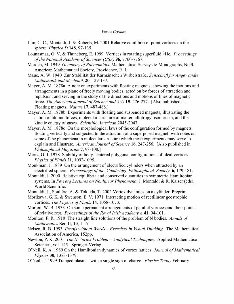
Vortex Crystals
63
Lim, C. C., Montaldi, J. & Roberts, M. 2001 Relative equilibria of point vortices on the sphere. Physica D 148, 97-135.
Lounasmaa, O. V, & Thuneberg, E. 1999 Vortices in rotating superfluid 3He. Proceedings of the National Academy of Sciences (USA) 96, 7760-7767.
Marden, M. 1949 Geometry of Polynomials. Mathematical Surveys & Monographs, No.3. American Mathematical Society, Providence, R. I.
Maue, A. W. 1940 Zur Stabilität der Kármánschen Wirbelstraße. Zeitschrift für Angewandte Mathematik und Mechanik 20, 129-137.
Mayer, A. M. 1878a A note on experiments with floating magnets; showing the motions and arrangements in a plane of freely moving bodies, acted on by forces of attraction and repulsion; and serving in the study of the directions and motions of lines of magnetic force. The American Journal of Science and Arts 15, 276-277. [Also published as: Floating magnets. Nature 17, 487-488.]
Mayer, A. M. 1878b Experiments with floating and suspended magnets, illustrating the action of atomic forces, molecular structure of matter, allotropy, isomerism, and the kinetic energy of gases. Scientific American 2045-2047.
Mayer, A. M. 1878c On the morphological laws of the configuration formed by magnets floating vertically and subjected to the attraction of a superposed magnet; with notes on some of the phenomena in molecular structure which these experiments may serve to explain and illustrate. American Journal of Science 16, 247-256. [Also published in Philosophical Magazine 7, 98-108.]
Mertz, G. J. 1978 Stability of body-centered polygonal configurations of ideal vortices. Physics of Fluids 21, 1092-1095.
Monkman, J. 1889 On the arrangement of electrified cylinders when attracted by an electrified sphere. Proceedings of the Cambridge Philosophical Society 6, 179-181.
Montaldi, J. 2000 Relative equilibria and conserved quantities in symmetric Hamiltonian systems. In Peyresq Lectures on Nonlinear Phenomena, J. Montaldi & R. Kaiser (eds), World Scientific.
Montaldi, J., Soulière, A. & Tokieda, T. 2002 Vortex dynamics on a cylinder. Preprint. Morikawa, G. K. & Swenson, E. V. 1971 Interacting motion of rectilinear geostrophic
vortices. The Physics of Fluids 14, 1058-1073. Morton, W. B. 1933 On some permanent arrangements of parallel vortices and their points
of relative rest. Proceedings of the Royal Irish Academy A 41, 94-101. Moulton, F. R. 1910 The straight line solutions of the problem of N bodies. Annals of
Mathematics Ser. II, 10, 1-17. Nelsen, R. B. 1993 Proofs without Words – Exercises in Visual Thinking. The Mathematical
Association of America, 152pp. Newton, P. K. 2001 The N-Vortex Problem – Analytical Techniques. Applied Mathematical
Sciences, vol. 145. Springer-Verlag. O’Neil, K. A. 1989 On the Hamiltonian dynamics of vortex lattices. Journal of Mathematical
Physics 30, 1373-1379. O’Neil, T. 1999 Trapped plasmas with a single sign of charge. Physics Today February
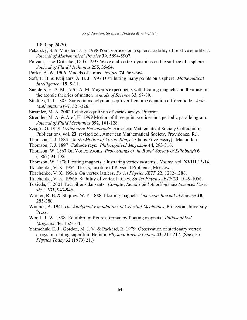
Aref, Newton, Stremler, Tokieda & Vainchtein
64
1999, pp.24-30. Pekarsky, S. & Marsden, J. E. 1998 Point vortices on a sphere: stability of relative equilibria.
Journal of Mathematical Physics 39, 5894-5907. Polvani, L. & Dritschel, D. G. 1993 Wave and vortex dynamics on the surface of a sphere.
Journal of Fluid Mechanics 255, 35-64. Porter, A. W. 1906 Models of atoms. Nature 74, 563-564. Saff, E. B. & Kuijlaars, A. B. J. 1997 Distributing many points on a sphere. Mathematical
Intelligencer 19, 5-11. Snelders, H. A. M. 1976 A. M. Mayer’s experiments with floating magnets and their use in
the atomic theories of matter. Annals of Science 33, 67-80. Stieltjes, T. J. 1885 Sur certains polynômes qui verifient une équation différentielle. Acta
Mathematica 6-7, 321-326. Stremler, M. A. 2002 Relative equilibria of vortex arrays. Preprint. Stremler, M. A. & Aref, H. 1999 Motion of three point vortices in a periodic parallelogram.
Journal of Fluid Mechanics 392, 101-128. Szegö , G. 1959 Orthogonal Polynomials. American Mathematical Society Colloquium
Publications, vol. 23, revised ed., American Mathematical Society, Providence, R.I. Thomson, J. J. 1883 On the Motion of Vortex Rings (Adams Prize Essay). Macmillan. Thomson, J. J. 1897 Cathode rays. Philosophical Magazine 44, 293-316. Thomson, W. 1867 On Vortex Atoms. Proceedings of the Royal Society of Edinburgh 6
(1867) 94-105. Thomson, W. 1878 Floating magnets [illustrating vortex systems]. Nature, vol. XVIII 13-14. Tkachenko, V. K. 1964 Thesis, Institute of Physical Problems, Moscow. Tkachenko, V. K. 1966a On vortex lattices. Soviet Physics JETP 22, 1282-1286. Tkachenko, V. K. 1966b Stability of vortex lattices. Soviet Physics JETP 23, 1049-1056. Tokieda, T. 2001 Tourbillons dansants. Comptes Rendus de l’Académie des Sciences Paris
sér.I 333, 943-946. Warder, R. B. & Shipley, W. P. 1888 Floating magnets. American Journal of Science 20,
285-288. Wintner, A. 1941 The Analytical Foundations of Celestial Mechanics. Princeton University
Press. Wood, R. W. 1898 Equilibrium figures formed by floating magnets. Philosophical
Magazine 46, 162-164. Yarmchuk, E. J., Gordon, M. J. V. & Packard, R. 1979 Observation of stationary vortex
arrays in rotating superfluid Helium Physical Review Letters 43, 214-217. (See also Physics Today 32 (1979) 21.)
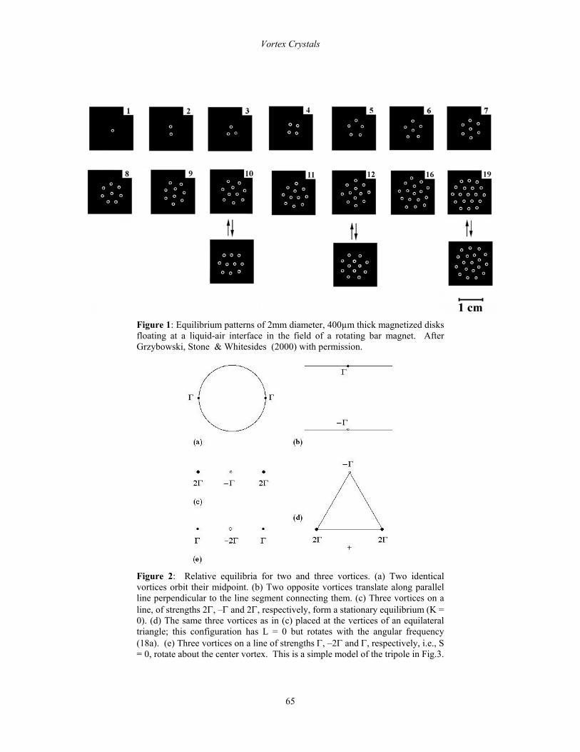
Vortex Crystals
65
Figure 1: Equilibrium patterns of 2mm diameter, 400µm thick magnetized disks floating at a liquid-air interface in the field of a rotating bar magnet. After Grzybowski, Stone & Whitesides (2000) with permission.
Figure 2: Relative equilibria for two and three vortices. (a) Two identical vortices orbit their midpoint. (b) Two opposite vortices translate along parallel line perpendicular to the line segment connecting them. (c) Three vortices on a line, of strengths 2Γ, –Γ and 2Γ, respectively, form a stationary equilibrium (K = 0). (d) The same three vortices as in (c) placed at the vertices of an equilateral triangle; this configuration has L = 0 but rotates with the angular frequency (18a). (e) Three vortices on a line of strengths Γ, –2Γ and Γ, respectively, i.e., S = 0, rotate about the center vortex. This is a simple model of the tripole in Fig.3.

Aref, Newton, Stremler, Tokieda & Vainchtein
66
Figure 3: The vortex ‘tripole’ found experimentally by van Heijst, Kloosterziel & Williams (1991). Courtesy of G. J. van Heijst; reproduced with permission.
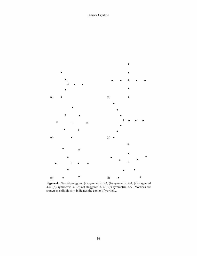
Vortex Crystals
67
67
(a)
+
(b)
+
(c)
+
(d)
+
(e)
+
(f)
+
Figure 4: Nested polygons. (a) symmetric 3-3; (b) symmetric 4-4; (c) staggered 4-4; (d) symmetric 3-3-3; (e) staggered 3-3-3; (f) symmetric 5-5. Vortices are shown as solid dots; + indicates the center of vorticity.
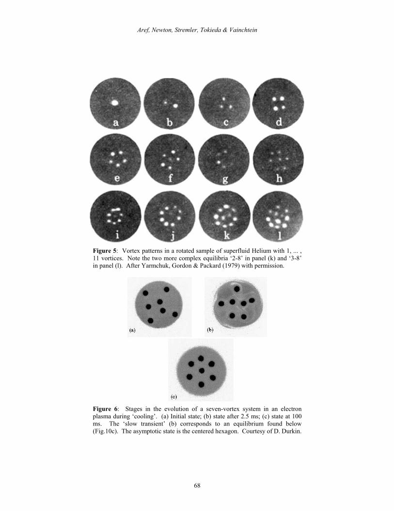
Aref, Newton, Stremler, Tokieda & Vainchtein
68
Figure 5: Vortex patterns in a rotated sample of superfluid Helium with 1, ... , 11 vortices. Note the two more complex equilibria ‘2-8’ in panel (k) and ‘3-8’ in panel (l). After Yarmchuk, Gordon & Packard (1979) with permission.
Figure 6: Stages in the evolution of a seven-vortex system in an electron plasma during ‘cooling’. (a) Initial state; (b) state after 2.5 ms; (c) state at 100 ms. The ‘slow transient’ (b) corresponds to an equilibrium found below (Fig.10c). The asymptotic state is the centered hexagon. Courtesy of D. Durkin.
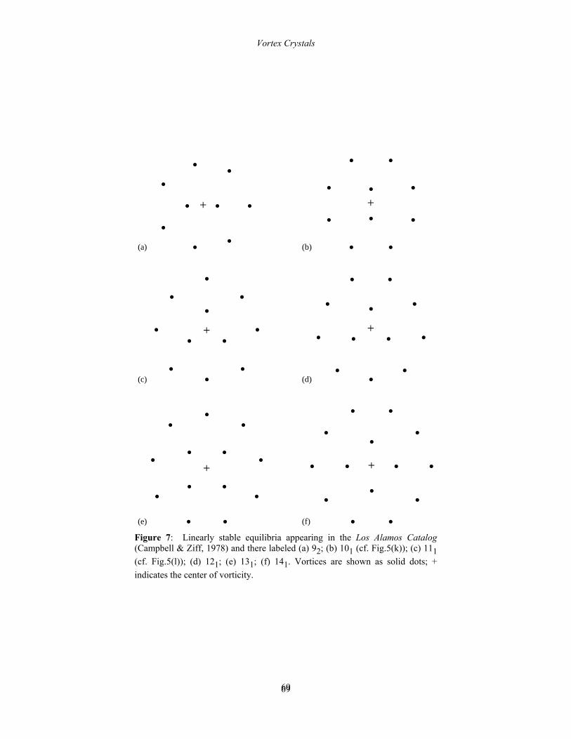
Vortex Crystals
69
69
(a)
+
(b)
+
(c)
+
(d)
+
(e)
+
(f)
+
Figure 7: Linearly stable equilibria appearing in the Los Alamos Catalog (Campbell & Ziff, 1978) and there labeled (a) 92; (b) 101 (cf. Fig.5(k)); (c) 111 (cf. Fig.5(l)); (d) 121; (e) 131; (f) 141. Vortices are shown as solid dots; + indicates the center of vorticity.
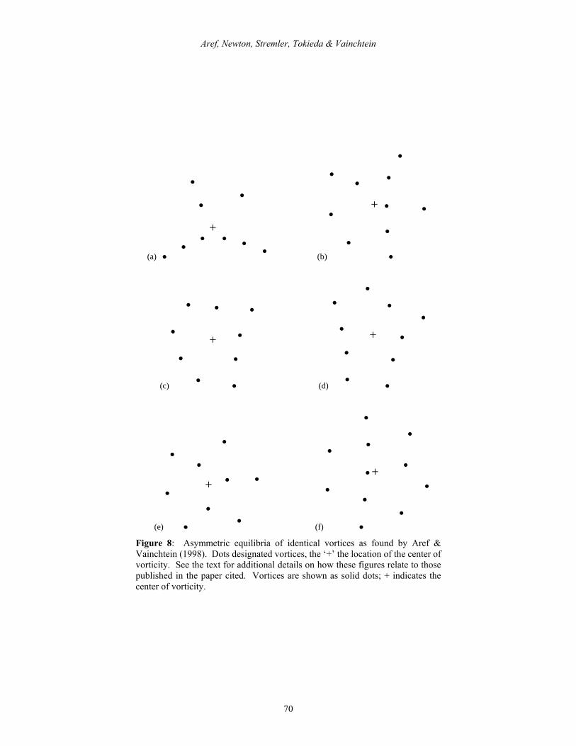
Aref, Newton, Stremler, Tokieda & Vainchtein
70
(a)
+
(b)
+
(c)
+
(d)
+
(e)
+
(f)
+
Figure 8: Asymmetric equilibria of identical vortices as found by Aref & Vainchtein (1998). Dots designated vortices, the ‘+’ the location of the center of vorticity. See the text for additional details on how these figures relate to those published in the paper cited. Vortices are shown as solid dots; + indicates the center of vorticity.
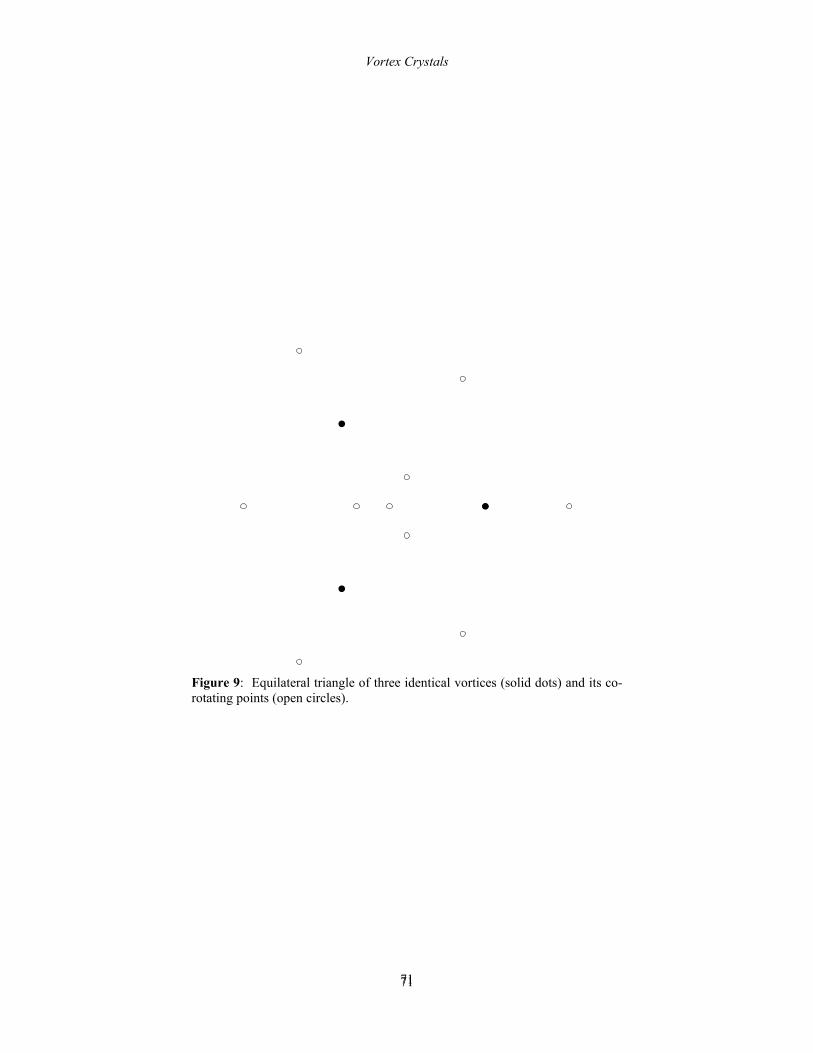
Vortex Crystals
71
71
Figure 9: Equilateral triangle of three identical vortices (solid dots) and its co-rotating points (open circles).
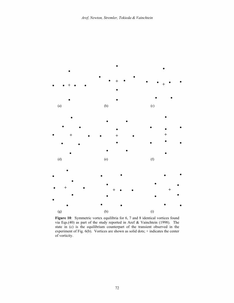
Aref, Newton, Stremler, Tokieda & Vainchtein
72
++
+
(a) (b) (c)
+ + +
(d) (e) (f)
+ + +
(g) (h) (i) Figure 10: Symmetric vortex equilibria for 6, 7 and 8 identical vortices found via Eqs.(40) as part of the study reported in Aref & Vainchtein (1998). The state in (c) is the equilibrium counterpart of the transient observed in the experiment of Fig. 6(b). Vortices are shown as solid dots; + indicates the center of vorticity.
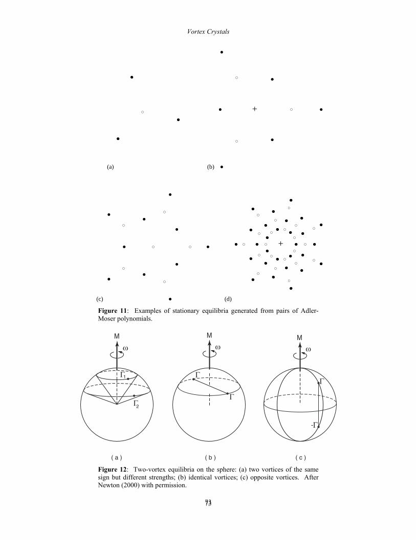
Vortex Crystals
73
73
(a) (b)
+
(c) (d)
+
Figure 11: Examples of stationary equilibria generated from pairs of Adler-Moser polynomials.
1
2
( a ) ( b ) ( c )
Μ Μ Μ
Figure 12: Two-vortex equilibria on the sphere: (a) two vortices of the same sign but different strengths; (b) identical vortices; (c) opposite vortices. After Newton (2000) with permission.
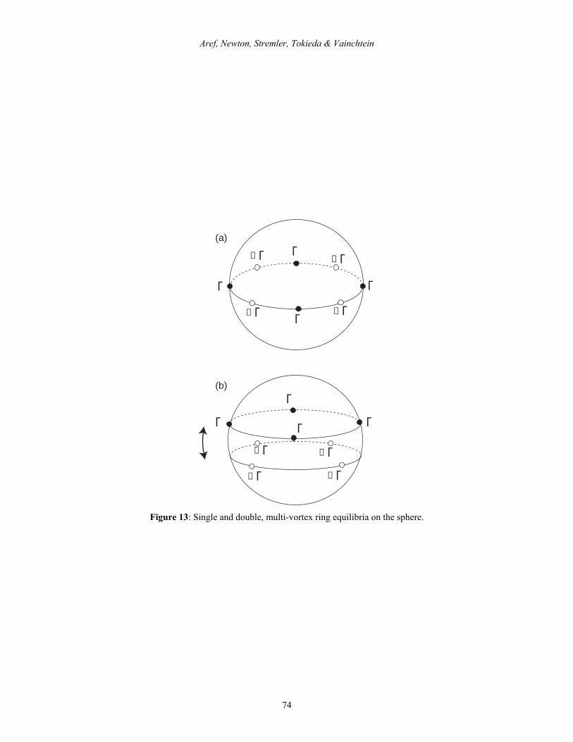
Aref, Newton, Stremler, Tokieda & Vainchtein
74
Γ
Γ
Γ
Γ
Γ−Γ−
Γ− Γ−
Γ
ΓΓ Γ
Γ−Γ−
Γ−Γ−
(a)
(b)
Figure 13: Single and double, multi-vortex ring equilibria on the sphere.
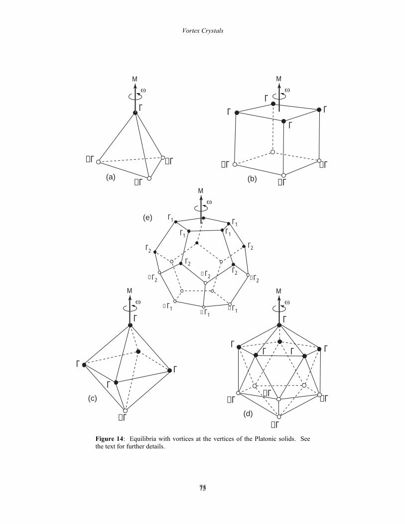
Vortex Crystals
75
75
(a) (b)
(c)
(d)
Γ Γ
ΓΓ
Γ
Γ
ΓΓ
Γ
Γ
ΓΓ Γ
−Γ
−Γ
−Γ
−Γ
−Γ
−Γ−Γ
−Γ −Γ
−Γ
−Γ
Γ1Γ1Γ1
Γ1
Γ1−Γ1−Γ1−
Γ2
Γ2
Γ2
Γ2
Γ− 2Γ− 2Γ2
(e)
−
Γ
Μ Μ
Μ
Μ Μ
Figure 14: Equilibria with vortices at the vertices of the Platonic solids. See the text for further details.
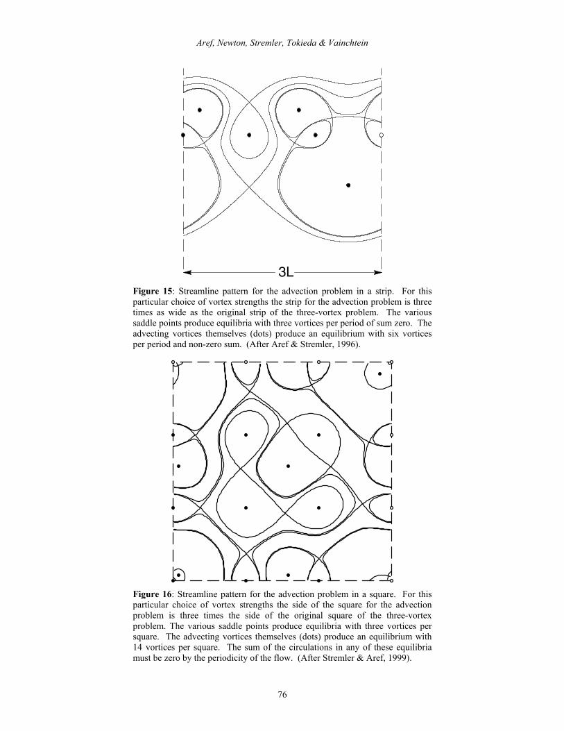
Aref, Newton, Stremler, Tokieda & Vainchtein
76
3L Figure 15: Streamline pattern for the advection problem in a strip. For this particular choice of vortex strengths the strip for the advection problem is three times as wide as the original strip of the three-vortex problem. The various saddle points produce equilibria with three vortices per period of sum zero. The advecting vortices themselves (dots) produce an equilibrium with six vortices per period and non-zero sum. (After Aref & Stremler, 1996).
Figure 16: Streamline pattern for the advection problem in a square. For this particular choice of vortex strengths the side of the square for the advection problem is three times the side of the original square of the three-vortex problem. The various saddle points produce equilibria with three vortices per square. The advecting vortices themselves (dots) produce an equilibrium with 14 vortices per square. The sum of the circulations in any of these equilibria must be zero by the periodicity of the flow. (After Stremler & Aref, 1999).

List of Recent TAM Reports
No. Authors Title Date
924 Adrian, R. J., C. D. Meinhart, and C. D. Tomkins
Vortex organization in the outer region of the turbulent boundary layer—Journal of Fluid Mechanics 422, 1–53 (2000)
Nov. 1999
925 Riahi, D. N., and A. T. Hsui
Finite amplitude thermal convection with variable gravity—International Journal of Mathematics and Mathematical Sciences 25, 153–165 (2001)
Dec. 1999
926 Kwok, W. Y., R. D. Moser, and J. Jiménez
A critical evaluation of the resolution properties of B-spline and compact finite difference methods—Journal of Computational Physics (submitted)
Feb. 2000
927 Ferry, J. P., and S. Balachandar
A fast Eulerian method for two-phase flow—International Journal of Multiphase Flow, in press (2000)
Feb. 2000
928 Thoroddsen, S. T., and K. Takehara
The coalescence–cascade of a drop—Physics of Fluids 12, 1257–1265 (2000)
Feb. 2000
929 Liu, Z.-C., R. J. Adrian, and T. J. Hanratty
Large-scale modes of turbulent channel flow: Transport and structure—Journal of Fluid Mechanics 448, 53–80 (2001)
Feb. 2000
930 Borodai, S. G., and R. D. Moser
The numerical decomposition of turbulent fluctuations in a compressible boundary layer—Theoretical and Computational Fluid Dynamics (submitted)
Mar. 2000
931 Balachandar, S., and F. M. Najjar
Optimal two-dimensional models for wake flows—Physics of Fluids, in press (2000)
Mar. 2000
932 Yoon, H. S., K. V. Sharp, D. F. Hill, R. J. Adrian, S. Balachandar, M. Y. Ha, and K. Kar
Integrated experimental and computational approach to simulation of flow in a stirred tank—Chemical Engineering Sciences 56, 6635–6649 (2001)
Mar. 2000
933 Sakakibara, J., Hishida, K., and W. R. C. Phillips
On the vortical structure in a plane impinging jet—Journal of Fluid Mechanics 434, 273–300 (2001)
Apr. 2000
934 Phillips, W. R. C. Eulerian space–time correlations in turbulent shear flows—Physics of Fluids 12, 2056–2064 (2000)
Apr. 2000
935 Hsui, A. T., and D. N. Riahi
Onset of thermal–chemical convection with crystallization within a binary fluid and its geological implications—Geochemistry, Geophysics, Geosystems 2, 2000GC000075 (2001)
Apr. 2000
936 Cermelli, P., E. Fried, and S. Sellers
Configurational stress, yield, and flow in rate-independent plasticity—Proceedings of the Royal Society of London A 457, 1447–1467 (2001)
Apr. 2000
937 Adrian, R. J., C. Meneveau, R. D. Moser, and J. J. Riley
Final report on ‘Turbulence Measurements for Large-Eddy Simulation’ workshop
Apr. 2000
938 Bagchi, P., and S. Balachandar
Linearly varying ambient flow past a sphere at finite Reynolds number—Part 1: Wake structure and forces in steady straining flow
Apr. 2000
939 Gioia, G., A. DeSimone, M. Ortiz, and A. M. Cuitiño
Folding energetics in thin-film diaphragms—Proceedings of the Royal Society of London A 458, 1223–1229 (2002)
Apr. 2000
940 Chaïeb, S., and G. H. McKinley
Mixing immiscible fluids: Drainage induced cusp formation May 2000
941 Thoroddsen, S. T., and A. Q. Shen
Granular jets—Physics of Fluids 13, 4–6 (2001) May 2000
942 Riahi, D. N. Non-axisymmetric chimney convection in a mushy layer under a high-gravity environment—In Centrifugal Materials Processing (L. L. Regel and W. R. Wilcox, eds.), 295–302 (2001)
May 2000
943 Christensen, K. T., S. M. Soloff, and R. J. Adrian
PIV Sleuth: Integrated particle image velocimetry interrogation/validation software
May 2000
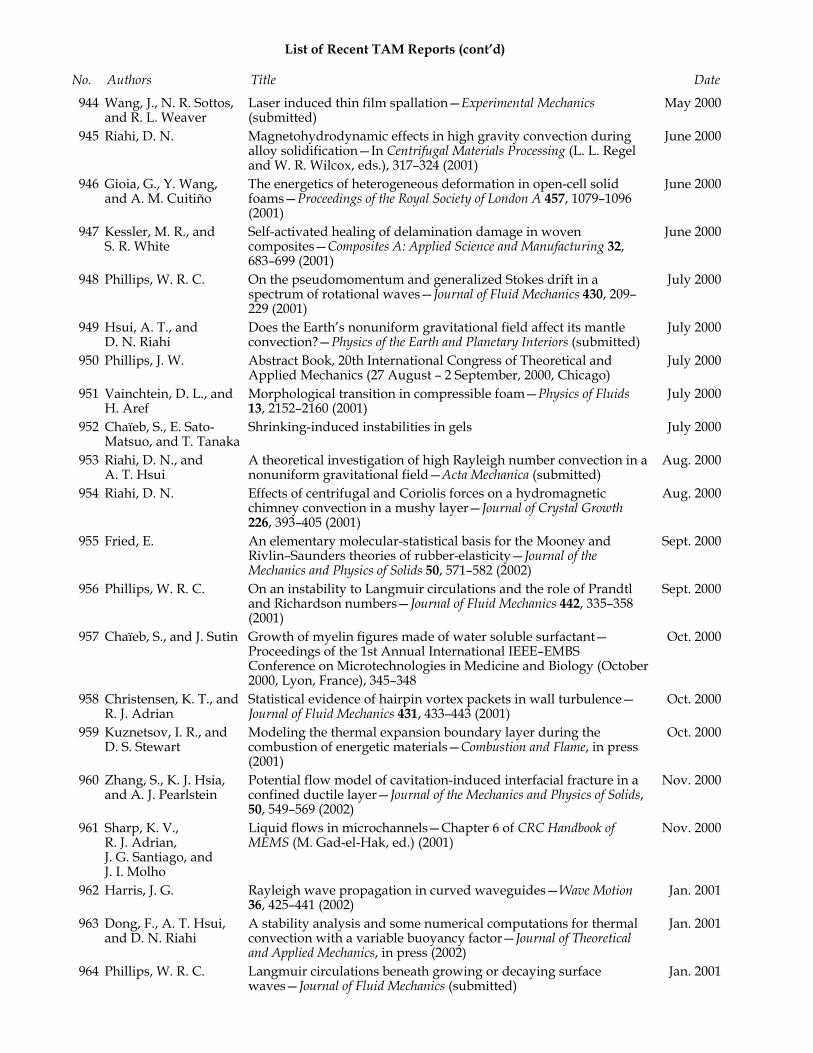
List of Recent TAM Reports (cont’d)
No. Authors Title Date 944 Wang, J., N. R. Sottos,
and R. L. Weaver Laser induced thin film spallation—Experimental Mechanics (submitted)
May 2000
945 Riahi, D. N. Magnetohydrodynamic effects in high gravity convection during alloy solidification—In Centrifugal Materials Processing (L. L. Regel and W. R. Wilcox, eds.), 317–324 (2001)
June 2000
946 Gioia, G., Y. Wang, and A. M. Cuitiño
The energetics of heterogeneous deformation in open-cell solid foams—Proceedings of the Royal Society of London A 457, 1079–1096 (2001)
June 2000
947 Kessler, M. R., and S. R. White
Self-activated healing of delamination damage in woven composites—Composites A: Applied Science and Manufacturing 32, 683–699 (2001)
June 2000
948 Phillips, W. R. C. On the pseudomomentum and generalized Stokes drift in a spectrum of rotational waves—Journal of Fluid Mechanics 430, 209–229 (2001)
July 2000
949 Hsui, A. T., and D. N. Riahi
Does the Earth’s nonuniform gravitational field affect its mantle convection?—Physics of the Earth and Planetary Interiors (submitted)
July 2000
950 Phillips, J. W. Abstract Book, 20th International Congress of Theoretical and Applied Mechanics (27 August – 2 September, 2000, Chicago)
July 2000
951 Vainchtein, D. L., and H. Aref
Morphological transition in compressible foam—Physics of Fluids 13, 2152–2160 (2001)
July 2000
952 Chaïeb, S., E. Sato-Matsuo, and T. Tanaka
Shrinking-induced instabilities in gels July 2000
953 Riahi, D. N., and A. T. Hsui
A theoretical investigation of high Rayleigh number convection in a nonuniform gravitational field—Acta Mechanica (submitted)
Aug. 2000
954 Riahi, D. N. Effects of centrifugal and Coriolis forces on a hydromagnetic chimney convection in a mushy layer—Journal of Crystal Growth 226, 393–405 (2001)
Aug. 2000
955 Fried, E. An elementary molecular-statistical basis for the Mooney and Rivlin–Saunders theories of rubber-elasticity—Journal of the Mechanics and Physics of Solids 50, 571–582 (2002)
Sept. 2000
956 Phillips, W. R. C. On an instability to Langmuir circulations and the role of Prandtl and Richardson numbers—Journal of Fluid Mechanics 442, 335–358 (2001)
Sept. 2000
957 Chaïeb, S., and J. Sutin Growth of myelin figures made of water soluble surfactant—Proceedings of the 1st Annual International IEEE–EMBS Conference on Microtechnologies in Medicine and Biology (October 2000, Lyon, France), 345–348
Oct. 2000
958 Christensen, K. T., and R. J. Adrian
Statistical evidence of hairpin vortex packets in wall turbulence—Journal of Fluid Mechanics 431, 433–443 (2001)
Oct. 2000
959 Kuznetsov, I. R., and D. S. Stewart
Modeling the thermal expansion boundary layer during the combustion of energetic materials—Combustion and Flame, in press (2001)
Oct. 2000
960 Zhang, S., K. J. Hsia, and A. J. Pearlstein
Potential flow model of cavitation-induced interfacial fracture in a confined ductile layer—Journal of the Mechanics and Physics of Solids, 50, 549–569 (2002)
Nov. 2000
961 Sharp, K. V., R. J. Adrian, J. G. Santiago, and J. I. Molho
Liquid flows in microchannels—Chapter 6 of CRC Handbook of MEMS (M. Gad-el-Hak, ed.) (2001)
Nov. 2000
962 Harris, J. G. Rayleigh wave propagation in curved waveguides—Wave Motion 36, 425–441 (2002)
Jan. 2001
963 Dong, F., A. T. Hsui, and D. N. Riahi
A stability analysis and some numerical computations for thermal convection with a variable buoyancy factor—Journal of Theoretical and Applied Mechanics, in press (2002)
Jan. 2001
964 Phillips, W. R. C. Langmuir circulations beneath growing or decaying surface waves—Journal of Fluid Mechanics (submitted)
Jan. 2001
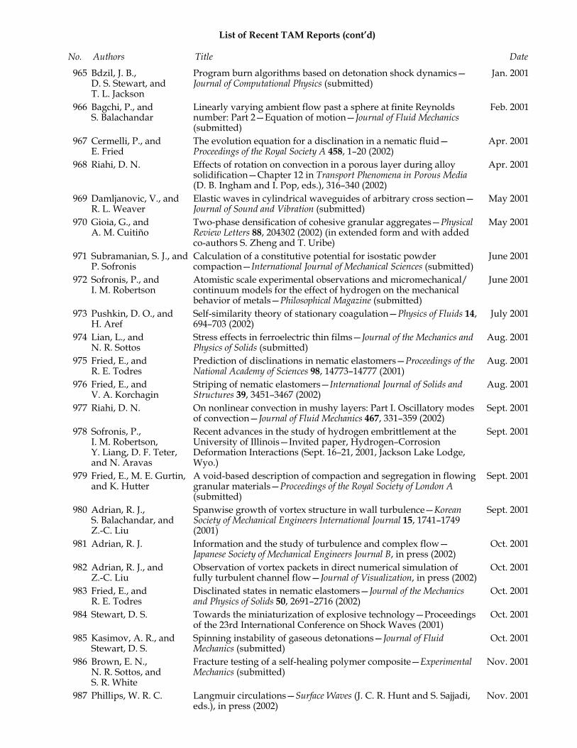
List of Recent TAM Reports (cont’d)
No. Authors Title Date 965 Bdzil, J. B.,
D. S. Stewart, and T. L. Jackson
Program burn algorithms based on detonation shock dynamics—Journal of Computational Physics (submitted)
Jan. 2001
966 Bagchi, P., and S. Balachandar
Linearly varying ambient flow past a sphere at finite Reynolds number: Part 2—Equation of motion—Journal of Fluid Mechanics (submitted)
Feb. 2001
967 Cermelli, P., and E. Fried
The evolution equation for a disclination in a nematic fluid—Proceedings of the Royal Society A 458, 1–20 (2002)
Apr. 2001
968 Riahi, D. N. Effects of rotation on convection in a porous layer during alloy solidification—Chapter 12 in Transport Phenomena in Porous Media (D. B. Ingham and I. Pop, eds.), 316–340 (2002)
Apr. 2001
969 Damljanovic, V., and R. L. Weaver
Elastic waves in cylindrical waveguides of arbitrary cross section—Journal of Sound and Vibration (submitted)
May 2001
970 Gioia, G., and A. M. Cuitiño
Two-phase densification of cohesive granular aggregates—Physical Review Letters 88, 204302 (2002) (in extended form and with added co-authors S. Zheng and T. Uribe)
May 2001
971 Subramanian, S. J., and P. Sofronis
Calculation of a constitutive potential for isostatic powder compaction—International Journal of Mechanical Sciences (submitted)
June 2001
972 Sofronis, P., and I. M. Robertson
Atomistic scale experimental observations and micromechanical/ continuum models for the effect of hydrogen on the mechanical behavior of metals—Philosophical Magazine (submitted)
June 2001
973 Pushkin, D. O., and H. Aref
Self-similarity theory of stationary coagulation—Physics of Fluids 14, 694–703 (2002)
July 2001
974 Lian, L., and N. R. Sottos
Stress effects in ferroelectric thin films—Journal of the Mechanics and Physics of Solids (submitted)
Aug. 2001
975 Fried, E., and R. E. Todres
Prediction of disclinations in nematic elastomers—Proceedings of the National Academy of Sciences 98, 14773–14777 (2001)
Aug. 2001
976 Fried, E., and V. A. Korchagin
Striping of nematic elastomers—International Journal of Solids and Structures 39, 3451–3467 (2002)
Aug. 2001
977 Riahi, D. N. On nonlinear convection in mushy layers: Part I. Oscillatory modes of convection—Journal of Fluid Mechanics 467, 331–359 (2002)
Sept. 2001
978 Sofronis, P., I. M. Robertson, Y. Liang, D. F. Teter, and N. Aravas
Recent advances in the study of hydrogen embrittlement at the University of Illinois—Invited paper, Hydrogen–Corrosion Deformation Interactions (Sept. 16–21, 2001, Jackson Lake Lodge, Wyo.)
Sept. 2001
979 Fried, E., M. E. Gurtin, and K. Hutter
A void-based description of compaction and segregation in flowing granular materials—Proceedings of the Royal Society of London A (submitted)
Sept. 2001
980 Adrian, R. J., S. Balachandar, and Z.-C. Liu
Spanwise growth of vortex structure in wall turbulence—Korean Society of Mechanical Engineers International Journal 15, 1741–1749 (2001)
Sept. 2001
981 Adrian, R. J. Information and the study of turbulence and complex flow—Japanese Society of Mechanical Engineers Journal B, in press (2002)
Oct. 2001
982 Adrian, R. J., and Z.-C. Liu
Observation of vortex packets in direct numerical simulation of fully turbulent channel flow—Journal of Visualization, in press (2002)
Oct. 2001
983 Fried, E., and R. E. Todres
Disclinated states in nematic elastomers—Journal of the Mechanics and Physics of Solids 50, 2691–2716 (2002)
Oct. 2001
984 Stewart, D. S. Towards the miniaturization of explosive technology—Proceedings of the 23rd International Conference on Shock Waves (2001)
Oct. 2001
985 Kasimov, A. R., and Stewart, D. S.
Spinning instability of gaseous detonations—Journal of Fluid Mechanics (submitted)
Oct. 2001
986 Brown, E. N., N. R. Sottos, and S. R. White
Fracture testing of a self-healing polymer composite—Experimental Mechanics (submitted)
Nov. 2001
987 Phillips, W. R. C. Langmuir circulations—Surface Waves (J. C. R. Hunt and S. Sajjadi, eds.), in press (2002)
Nov. 2001
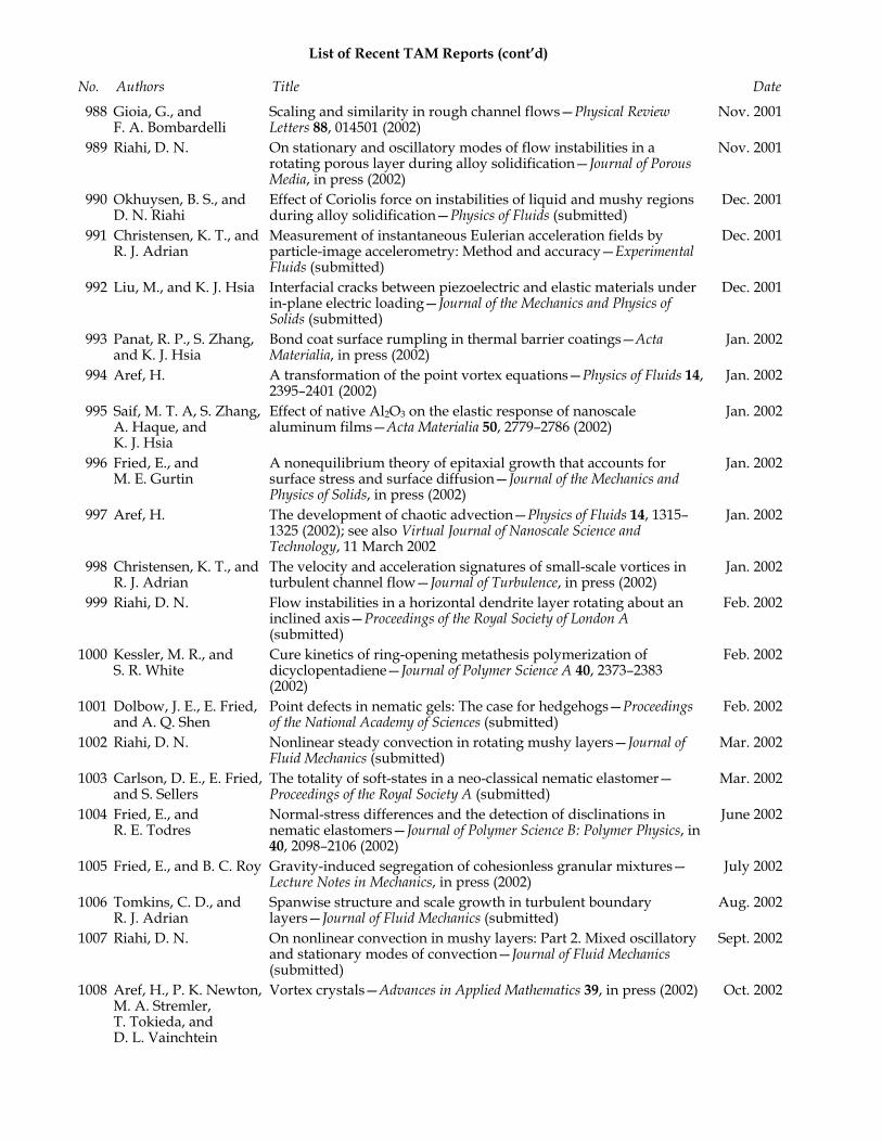
List of Recent TAM Reports (cont’d)
No. Authors Title Date 988 Gioia, G., and
F. A. Bombardelli Scaling and similarity in rough channel flows—Physical Review Letters 88, 014501 (2002)
Nov. 2001
989 Riahi, D. N. On stationary and oscillatory modes of flow instabilities in a rotating porous layer during alloy solidification—Journal of Porous Media, in press (2002)
Nov. 2001
990 Okhuysen, B. S., and D. N. Riahi
Effect of Coriolis force on instabilities of liquid and mushy regions during alloy solidification—Physics of Fluids (submitted)
Dec. 2001
991 Christensen, K. T., and R. J. Adrian
Measurement of instantaneous Eulerian acceleration fields by particle-image accelerometry: Method and accuracy—Experimental Fluids (submitted)
Dec. 2001
992 Liu, M., and K. J. Hsia Interfacial cracks between piezoelectric and elastic materials under in-plane electric loading—Journal of the Mechanics and Physics of Solids (submitted)
Dec. 2001
993 Panat, R. P., S. Zhang, and K. J. Hsia
Bond coat surface rumpling in thermal barrier coatings—Acta Materialia, in press (2002)
Jan. 2002
994 Aref, H. A transformation of the point vortex equations—Physics of Fluids 14, 2395–2401 (2002)
Jan. 2002
995 Saif, M. T. A, S. Zhang, A. Haque, and K. J. Hsia
Effect of native Al2O3 on the elastic response of nanoscale aluminum films—Acta Materialia 50, 2779–2786 (2002)
Jan. 2002
996 Fried, E., and M. E. Gurtin
A nonequilibrium theory of epitaxial growth that accounts for surface stress and surface diffusion—Journal of the Mechanics and Physics of Solids, in press (2002)
Jan. 2002
997 Aref, H. The development of chaotic advection—Physics of Fluids 14, 1315–1325 (2002); see also Virtual Journal of Nanoscale Science and Technology, 11 March 2002
Jan. 2002
998 Christensen, K. T., and R. J. Adrian
The velocity and acceleration signatures of small-scale vortices in turbulent channel flow—Journal of Turbulence, in press (2002)
Jan. 2002
999 Riahi, D. N. Flow instabilities in a horizontal dendrite layer rotating about an inclined axis—Proceedings of the Royal Society of London A (submitted)
Feb. 2002
1000 Kessler, M. R., and S. R. White
Cure kinetics of ring-opening metathesis polymerization of dicyclopentadiene—Journal of Polymer Science A 40, 2373–2383 (2002)
Feb. 2002
1001 Dolbow, J. E., E. Fried, and A. Q. Shen
Point defects in nematic gels: The case for hedgehogs—Proceedings of the National Academy of Sciences (submitted)
Feb. 2002
1002 Riahi, D. N. Nonlinear steady convection in rotating mushy layers—Journal of Fluid Mechanics (submitted)
Mar. 2002
1003 Carlson, D. E., E. Fried, and S. Sellers
The totality of soft-states in a neo-classical nematic elastomer—Proceedings of the Royal Society A (submitted)
Mar. 2002
1004 Fried, E., and R. E. Todres
Normal-stress differences and the detection of disclinations in nematic elastomers—Journal of Polymer Science B: Polymer Physics, in 40, 2098–2106 (2002)
June 2002
1005 Fried, E., and B. C. Roy Gravity-induced segregation of cohesionless granular mixtures—Lecture Notes in Mechanics, in press (2002)
July 2002
1006 Tomkins, C. D., and R. J. Adrian
Spanwise structure and scale growth in turbulent boundary layers—Journal of Fluid Mechanics (submitted)
Aug. 2002
1007 Riahi, D. N. On nonlinear convection in mushy layers: Part 2. Mixed oscillatory and stationary modes of convection—Journal of Fluid Mechanics (submitted)
Sept. 2002
1008 Aref, H., P. K. Newton, M. A. Stremler, T. Tokieda, and D. L. Vainchtein
Vortex crystals—Advances in Applied Mathematics 39, in press (2002) Oct. 2002