Approaches to Management and Farm Business Success

William D. McBride and James D. Johnson

Economic Research Service, U.S. Department of Agriculture, Washington, DC

Selected Paper prepared for presentation at the American Agricultural Economics Association Annual Meetings, Denver, Colorado, August 1-4, 2004.

The opinions and conclusions expressed here are those of the authors and may not represent the views of the U.S. Department of Agriculture. Do not reproduce, quote, cite, or distribute without permission of the authors.

Approaches to Management and Farm Business Success

During much of 1998 through 2002 many U.S. farmers faced an economic pinch of low

commodity prices and high input costs. Prices for most field crops were low throughout this

period as average corn prices remained below $2.00 per bushel in most months, wheat prices

stayed below $3.00 per bushel, and soybean prices were mostly under $5.00 per bushel (U.S.

Department of Agriculture, National Agricultural Statistics Service). Likewise, average cotton

prices trended downward and bottomed at less than 30 cents per pound. Livestock prices were

highly variable during this period, with hog and milk prices near historic lows at times, below

$20 per hundredweight for hogs and nearly $11 per hundredweight for milk. To make matters

worse, an unanticipated increase in energy prices caused spikes in fuel and fertilizer costs, most

notable during the spring of 2001. Faced with this cost-price squeeze, the role of the farmer as a

business manager was critical as strategies were developed and implemented in an attempt to

maintain farm profitability.

Agricultural professionals have long recognized that differences in management result in

differences in the financial performance of farms facing similar resource and production

conditions. However, management is quite difficult to define and measure in order to isolate its

effect on farm business success. As a result, it is often omitted from the specification of models

attempting to explain variation in farm financial performance, resulting in bias of estimated

parameters. Even when management variables are specified in these models the same type of

problem may occur because of measurement error. Previous research provides no clear

consensus on what variables represent management or whether they accurately reflect the

2

manager’s ability or approach. Further, there has been little success made in linking

management with farm financial success or efficiency.

These issues are addressed in this study through a model relating farm financial success to

management approaches used by a sample of U.S. farmers collected for 2001. A methodology is

developed that relates latent management variables to farm financial performance measures and

evaluates their individual impacts on financial success. Objectives of this study are to (1)

describe the approaches to management that were employed by farmers, and (2) examine what

impact these management approaches had on the financial success of farm businesses. Results

of this analysis may provide useful information to farmers, lenders, consultants, and policy

makers about what management strategies can be used to guide farm businesses through difficult

times, to lessen their dependence on government support, and to improve the competitiveness of

U.S. farmers.

Previous Research

Several attempts have been made to relate management to farm business success. Typically,

management has been represented in regression models as a set of farm performance,

demographic, or production practice variables used as proxies for the unobserved level of

management. For example, Purdy, Langemeier, and Featherstone studied financial performance

on a sample of crop and livestock farmers using operator characteristics, and financial efficiency

and solvency variables as indicators of management. Mishra, El-Osta, and Johnson specified

operator education as a proxy for management ability in a model of financial performance on

cash grain farms. They also specified the ratio of operating expenses to farm production value as

3

representing the cost control aspect of management, and technology adoption variables as

indicative of innovativeness.

Kauffman and Tauer attempted to identify successful farm management strategies using records

from dairy farms. They specified output, cost, technology, and financial variables in a logit

model of financial success. Using the estimated coefficients on these variables, they concluded

that cost control, selective technology adoption, and financial leverage were important aspects of

successful dairy farm management. Mishra and Morehart also studied financial success on dairy

farms and found that various components of management, measured by operator education, cost

control, farm business organization, and risk management, were important to farm business

success.

In a concerted effort to model the effect of management ability on farm financial success, Ford

and Shonkwiler related 3 types, or factors, of latent management ability-financial, dairy, and

crop management-to financial performance on a sample of dairy farms. A structural equation

model was constructed using confirmatory factor analysis. The factor analysis determined how

the set of observed management variables, including various measures of farm efficiency, loaded

on (i.e., correlated with) each of the latent factors. The analysis illustrated the difficulties

involved with managing all facets of dairy farms, as the 3 factors were negatively correlated with

one another, and the results suggested that dairy management had the greatest payoff. The

authors also concluded that the latent variable approach was a promising tool for disentangling

management from other farm measures in determining factors necessary for farm financial

success.

4

More recent literature concerning successful farm management has focused on the importance of

strategic planning for positioning the farm business. Miller, Boehlje, and Dobbins characterize

strategic planning as a different way of thinking about management. In the past, farming success

depended primarily on the ability of management to develop an efficient operation, such as

achieving a cost of production lower than the industry average. The continued introduction of

new products and/or technologies has provided significant rewards for concentrating on

production or “doing things right.” Miller, Boehlje and Dobbins argue that while important,

efficient production will not be sufficient to assure success in an increasingly industrialized

environment. Their point is that the continued industrialization of farming makes strategic

decisions such as farm product mix, market linkages, financial structure, and relationships with

input suppliers and product buyers more important. In this environment success in farming will

continue to require that operations be efficient, but there will be a growing payoff to strategic

decisions or “doing the right things.”

A problem with using operator characteristics as proxies for management is that they only reflect

a potential management impact, and not the specific management approach or actions that were

taken. Also, specifying the level of management with efficiency measures, such as cost per unit

of output, raises the question of whether these variables can be considered exogenous in relation

to measures of financial performance. Management is specified in this study using the latent

variable approach, as in Ford and Shonkwiler, but this study uses specific data on farm

management actions rather than farm efficiency measures. Responses from a sample of farm

operations are used to describe management approaches in terms of managerial actions and to

5

characterize management in terms of what Miller, Boehlije and Dobbins describe as “the right

things to do.”

Data

Data used in this study come from the 2001 Agricultural Resource Management Survey

(ARMS). Each farm in the ARMS sample represents a known number of farms with similar

attributes so that weighting the data for each farm by the number of farms it represents provides

a basis for calculating estimates for the target population. The annual ARMS data include

detailed information about farm income and expenses, farm assets and debt, and farm and

operator characteristics, as well as information about the farm household.

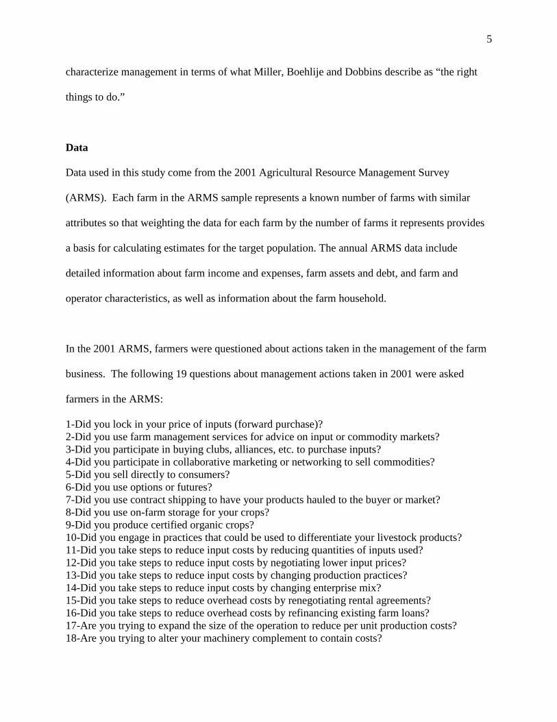
In the 2001 ARMS, farmers were questioned about actions taken in the management of the farm

business. The following 19 questions about management actions taken in 2001 were asked

farmers in the ARMS:

1-Did you lock in your price of inputs (forward purchase)? 2-Did you use farm management services for advice on input or commodity markets? 3-Did you participate in buying clubs, alliances, etc. to purchase inputs? 4-Did you participate in collaborative marketing or networking to sell commodities? 5-Did you sell directly to consumers? 6-Did you use options or futures? 7-Did you use contract shipping to have your products hauled to the buyer or market? 8-Did you use on-farm storage for your crops? 9-Did you produce certified organic crops? 10-Did you engage in practices that could be used to differentiate your livestock products? 11-Did you take steps to reduce input costs by reducing quantities of inputs used? 12-Did you take steps to reduce input costs by negotiating lower input prices? 13-Did you take steps to reduce input costs by changing production practices? 14-Did you take steps to reduce input costs by changing enterprise mix? 15-Did you take steps to reduce overhead costs by renegotiating rental agreements? 16-Did you take steps to reduce overhead costs by refinancing existing farm loans? 17-Are you trying to expand the size of the operation to reduce per unit production costs? 18-Are you trying to alter your machinery complement to contain costs?

6

19-Are you trying to adopt cost saving technologies to contain costs? Table 1 includes a summary of the management actions taken on different types of farms as

reported in the ARMS. Type of farm is designated as the commodity that provided the largest

share of production value in 2001. Many of the differences in management actions across farm

types reflect differences in the marketing methods used for the primary commodity. For

example, most vegetable farms reported selling directly to consumers, such as farmers’ markets

or other local retail establishments. A relatively large share of dairy farms reported the use of

contract shipping and on-farm storage, probably for milk. Likewise, cotton farms more often

participated in selling groups such as those associated with the warehouse system. Other notable

differences include the large share of cash grain farms that forward purchase inputs and store

grain on-farm, and that a higher proportion of cotton farms were refinancing loans and using

farm expansion to reduce costs than were other types of farms.

The analysis in this study was limited to the set of farms that reported the farm type as cash grain

(including oilseeds) production. This included 1,149 farms in the ARMS sample representing a

population of about 370,000 farms across the nation. Because relatively few cash grain farms

reported using management actions 9 (produce certified organic crops) and 10 (differentiate your

livestock products), these were omitted from the analysis.

Empirical Approach

To illustrate the empirical approach used in this study, consider the following regression

equation:

7

where Y is a measure of farm financial performance, X is a matrix of explanatory variables, V is

a matrix of the management action variables, and ε is a random disturbance assumed to be

normally distributed. It is hypothesized that the management action variables are not each

measuring unique approaches to management, but together are measuring a few underlying

factors, or constructs, that characterize management approaches. The technique of exploratory

factor analysis is appropriate when a number of variables are measured, and the number and

nature of the underlying factors that are responsible for covariation in the data are to be

identified.

Exploratory factor analysis was used to examine the pattern of intercorrelation among responses

to the set of management action questions in order to reduce their number and correlation1. A

factor is an unobserved, or hypothetical latent variable that is hypothesized to exist and to

influence certain observed variables that can be measured directly. The goal of factor analysis is

to explain the variance in the observed variables in terms of the underlying latent factors. The

latent variables are believed to be various approaches to management that are unobserved, but

are influenced by the observed variables measuring management actions taken by farmers. This

can be illustrated by the following regression equation:

1 Factor analysis can be used as a variable reduction technique that circumvents statistical problems associated with including all the management action variables in equation (1). One problem is that some management variables are likely to be highly correlated. The intercorrelation among explanatory variables would result in an upward bias of the variance estimates of the least squares estimators, β and γ, and thus generate unreliable tests of their statistical significance. The effect of measurement error associated with the management action variables may also be reduced by using factor analysis for variable reduction (Scott).

εVγXβY (1) ++=

8

where Vj is vector of values for the observed jth variable (i.e., management action), ak (k=1…q)

is a vector of regression coefficients (or weights) for factor k, Fkj is a vector of estimated

loadings of factor k on the jth variable, and the vector µj is similar to a residual, but known as the

j th variable’s unique factor (Hatcher). A critical decision in factor analysis is to determine the

appropriate number of meaningful factors, q, described by the data.

Once the appropriate number of meaningful factors is determined, the factor loadings can be

rotated to a final solution. Rotation refers to a linear transformation of the factor loadings to

simplify the factor structure and to achieve a more meaningful and interpretable solution. Factor

scores from the final solution can be estimated by:

where Fk is a vector of estimated factor scores for the kth factor (i.e., management approach), bj

(j=1…p) is a vector of scoring coefficients for variable j used in creating estimated factor score

k, and Vjk is a vector of standardized values for the observed jth variable (i.e., management

action).

The estimated factor scores are used to represent latent management approaches. Factor scores

are substituted for the management actions in equation (1), giving:

εψFXβY (4) k ++=

jqjq2j21j1j µFa...FaFaV (2) ++++=

pkp2k21k1k Vb...VbVbF (3) +++=

9

Regression coefficients on the k (k=1…q) factor scores (ψ) indicate the impact that each

approach to management identified in the factor analysis had on farm financial performance.

The impact of individual management actions on financial performance, shown by:

consists of 2 parts. The first part is the change in financial performance associated with each

factor score (ψ). The second part indicates how factor scores change in response to each

management action (bj).

Conducting a Factor Analysis

Factor analysis is a statistical technique widely used in psychology and other social sciences, and

is regarded as a necessity in some branches of psychology where tests or questionnaires are often

administered (Kline). Conducting a factor analysis involves a sequence of steps with somewhat

subjective decisions made along the way. The first step is the initial extraction of the factors.

The number of factors initially extracted will be equal to the number of variables being analyzed.

A critical decision is determining how many of these factors are meaningful and worthy of being

retained for rotation and interpretation. In general, only the first few factors account for

meaningful amounts of variance, and later factors account for only small amounts.

Options available for determining the meaningful number of factors include the scree test,

proportion of variance explained, and the interpretability criterion (Hatcher). With the scree test,

the eigenvalues associated with each factor are plotted and factors appearing before the break

between large and small eigenvalues are assumed to be meaningful factors. The second option

jjk

k

kbψ

V

F

F

Y

V

Y (5) ⋅=

∂∂⋅

∂∂=

∂∂

10

involves retaining a factor if it accounts for a certain (arbitrary) percentage of the variance in the

data, such as those with at least 5 or 10 percent. Probably the most important criterion for

solving the number of factors problem is the interpretability criterion: interpreting the substantive

meaning of the retained factors and verifying that the interpretation is consistent with what is

known about the constructs under investigation. A few rules to follow are (Hatcher): (1) do at

least 3 variables have significant loadings on each retained factor? (2) do variables loading on

the same factor share a conceptual meaning? and (3) do variables loading on different factors

measure different constructs?

In order to make interpretation of the retained factors easier, a linear transformation, called a

rotation, is performed on the factor solution. A major criticism of factor analysis is that there are

an infinite number of mathematically equivalent solutions resulting from factor rotation.

However, the solution that meets the “simple structure” criterion is generally regarded as the best

solution (Kline). A rotated factor pattern demonstrates simple structure when (1) most variables

have high loadings on one factor and near-zero loadings on others, and (2) each factor has high

loadings for some variables and near-zero loadings for others. The rotated factor solution yields

the rotated factor pattern matrix, including standardized regression coefficients that indicate the

factor loadings of the variables on the factors. Factor scores are developed from the regression

coefficients, and indicate an estimate of each subject’s standing on the underlying factor.

Model Specification

The impact of various approaches to management on farm financial performance is assessed by

statistically controlling for several other factors that may also affect financial performance. That

11

is, the effect of economic and environmental conditions and farm structural and operator

characteristics are accounted for in order to isolate the effect of management on farm financial

performance. By limiting the analysis to the set of farms in the data that reported the farm type

as cash grain production, differences in financial performance that can be attributed to the

commodity mix are diminished.

Estimated factor scores were used to represent different approaches to management and were

specified as explanatory variables in regression models of farm financial performance. Other

explanatory variables included many of the farm structural and operator variables shown in

previous studies to be related to farm financial performance (Mishra and Morehart; Mishra, El-

Osta, and Johnson; Purdy, Langemeier, and Featherstone). Variables regressed against measures

of farm financial performance included operator age (AGE) and education (EDUC), and whether

or not the operator reported farming as the primary occupation (OCUP) (table 2). Unlike other

studies where these operator characteristics were used to represent management level, these

variables were specified to isolate the impact that differences in human capital, including

operator goals (age and occupation) and formal training (education), had on financial

performance.

Operator risk preference was specified from the position on a scale of risk preferences (RISK),

where 0 implies risk adverse and 10 implies risk loving, indicated by the farm operator. Farm

size (SIZE), specialization (SPECIAL), land tenure (TENURE), and an indicator for the presence

of a livestock operation (LSTOCK) were specified to reflect differences in farm organization.

Farm size was also specified with a quadratic term (SIZESQ). Variables for geographic location

12

(HL, NC, NP, PG, EU, SS, FR, BR, and MP) were also included in the model to account for the

impact that differences in soil, climate, production practices, and pest pressures have on farm

finances.

Several measures of farm financial performance were specified as the dependent variable, but

results are reported for only two measures, modified net farm income and gross operating

margin2. Modified net farm income (MNFI) was measured from the ARMS data as:

MNFI = Net Farm Income (NFI) + interest expense

NFI = Gross farm income – total farm operating expenses (excluding marketing expenses)

Where:

Gross farm income = gross cash farm income + net change in inventory values + value of

farm consumption + imputed rental value of operators dwelling

Total farm operating expenses = total cash operating expenses + estimate of non-cash

expenses for paid labor + depreciation on farm assets

Gross operating margin (GOM) was measured using the ARMS data as:

GOM = Gross farm income – variable cash operating expenses

Net farm income has been used as a measure of financial performance in several studies (Mishra,

El-Osta, and Johnson; El-Osta and Johnson; Haden and Johnson; McBride and El-Osta). Net

farm income was modified in this study by adding back interest expenses so that variation in

farm debt did not influence the financial comparison among farms. MNFI is a comprehensive

13

measure of financial performance that would be influenced by most of the management actions

examined in this study. Gross operating margin has been used in other studies (e.g., McBride

and El-Osta) and was examined here because select management actions, such as marketing and

input use strategies, are likely to have a more measurable impact on gross operating margin.

This measure of financial performance is also less likely to be confounded by other factors that

influence net farm income. However, results from models specified with GOM, compared to

those using MNFI, provide a weaker test about the influence that various management actions

have on farm financial performance because MNFI is a more comprehensive measure of farm

business success.

Results

The maximum likelihood method was used to extract the initial factors in the factor analysis. An

oblique rotation with the promax method was used to transform the solution (Gorsuch).

Solutions from oblique rotations differ from those of orthogonal rotations in that the resulting

factors may be correlated with one another, and thus provide better results in those situations

where the actual underlying factors are truly correlated, as may occur with the management

approaches (Hatcher).

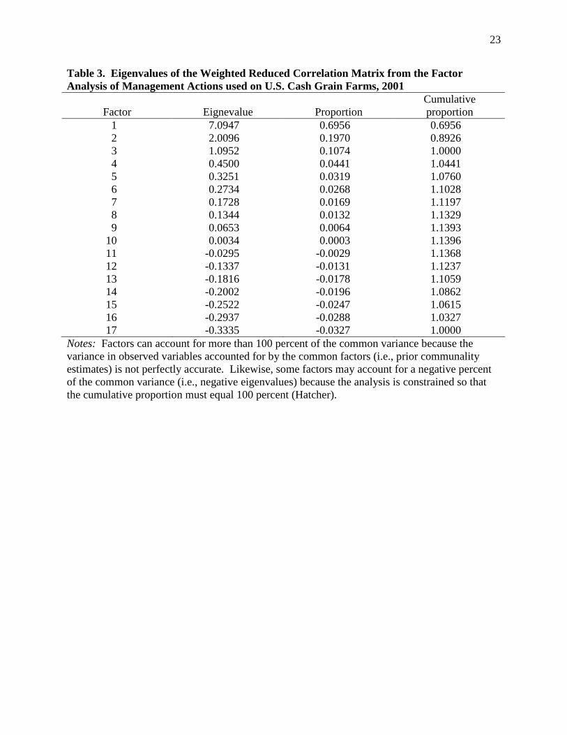
The scree test and the proportion of variance accounted for by various factors suggested that the

list of management actions could be described by 3 latent variables3. Eigenvalues for the

weighted reduced correlation matrix (weighted with the ARMS survey weights) are shown in

2 Other financial performance measures examined for this study were an estimate of operator labor and management income (net farm income less charges for unpaid labor and capital) and rate of return to assets. There was less of a relationship between these measures and the explanatory variables than for those reported in this study. 3 The scree plot of the eigenvalues is not shown due to space limitations.

14

table 3. The first factor accounted for about 70 percent of the variance, the second about 20

percent, and the third about 11 percent. No other subsequent factor accounted for more than 4

percent of the variance. Most importantly, the 3 factors were determined to be interpretable in a

manner that is consistent with constructs that indicate approaches to management.

The rotated factor pattern, shown in the form of standardized regression coefficients, is presented

in table 4. The factor pattern shows the characteristics of simple structure as most variables have

a high loading on one factor and much lower, near-zero in most cases, loadings on other factors.

Likewise, each factor has high loadings for some variables and near-zero loadings for most

others. In interpreting the rotated factor pattern, an item was said to load on a given factor if the

factor loading was 0.40 or greater for that factor, and was less than 0.40 for any other.

Using these criteria for determining factor loading, responses to the following 4 questions:

1-Did you lock in the price of inputs (forward purchase)? 2-Did you use farm management services for advice on input or commodity markets? 6-Did you use options or futures? 12-Did you take steps to reduce input costs by negotiating lower input prices? were found to load on the first factor. These questions refer to management actions for

establishing input and output prices, and thus the factor was labeled as the “price negotiation”

approach to management. Responses to the following 3 questions:

17-Are you trying to expand the size of your operation to reduce per unit production costs? 18-Are you trying to alter your machinery complement to contain costs? 19-Are you trying to adopt cost saving technologies to contain costs? loaded on the second factor. These questions refer to management actions that involve

investments to lower costs, and thus the factor was labeled as the “long-term cost control”

approach to management. Responses to the following 3 questions:

15

11-Did you take steps to reduce input costs by reducing quantities of inputs used? 13-Did you take steps to reduce input costs by changing production practices? 14-Did you take steps to reduce input costs by changing enterprise mix? were found to load on the third factor. These questions refer to management actions that involve

adjusting input use to control costs, and thus the factor was labeled as the “input adjustment”

approach to management.

Results of the financial performance regression models, with modified net farm income (MNFI)

and gross operating margin (GOM) as the dependent variables, are presented in table 5. The

overall model fit was best for the GOM model with an R-squared of 0.31, compared with 0.15

for the MNFI model. Thus, the model was better at explaining the variation in GOM relative to

MNFI. This is not surprising because of the additional “overhead” or fixed costs that influence

MNFI, taxes, insurance, rent, and depreciation, that were not included in the calculation of GOM.

The regression results indicate that farm size was statistically significant in both models with

MNFI and GOM increasing with farm size at a decreasing rate. Predicted values for both MNFI

and GOM reach a maximum at a farm size of more than $40 million in value of product, far

beyond the mean of $114,000 and approaching the maximum data value. The parameter

estimate on the occupation variable was also statistically significant in both models, indicating

that farmers reporting a major occupation of farming had higher financial performance measures

than did farmers who reported a major occupation as either retired or off-farm employment. The

coefficients indicate that a farming occupation was associated with about $17,000 more in MNFI

and $25,000 more in GOM. A few regional variables were also statistically significant in the

models. These coefficients indicate the difference in financial performance measures between

16

each region and the Heartland, the deleted group. For example, both MNFI and GOM were

higher due to location in the Northern Plains relative to the Heartland, while location in the

Northern Crescent was associated with a lower MNFI relative to the Heartland.

The factor score indicating the level of price negotiation was positive and statistically significant

in both regression models. This means that a management approach emphasizing price setting

practices had a positive relationship with farm financial performance in 2001. The factor score

indicating a long-term cost control approach was not statistically significant in either model. It is

possible that one year of data is not sufficient to reflect the impact on financial performance that

is involved with this long-term management approach. The factor score for the input adjustment

approach was statistically significant and negative in the model of GOM. This suggests that a

management approach emphasizing reduced input use and altering production practices for cost

control was negatively associated with farm financial performance in 2001.

The change in financial performance associated with management actions that are part of each

statistically significant approach are shown in table 6. Because the management actions are 0,1

variables, the change in financial performance was computed as the difference in financial

measures computed at 1 and at 0, while holding other variables constant. This involved first

computing the factor scores when each management action was set to 1 and to 0, then computing

the impact of the factor scores on each financial measure, as shown in equation (5). The price

negotiation approach had a positive impact on financial performance, and the management action

with the greatest positive impact was locking in input prices (i.e., forward purchasing),

increasing MNFI by about $5,500 and GOM by $20,000 on average. Market advice from farm

17

management services, and marketing with options and futures increased MNFI and GOM by

about $4,000 and nearly $15,000, respectively. The input adjustment approach negatively

impacted GOM, and changing production practices to reduce input costs had the largest negative

impact, reducing GOM by an average of more than $10,000. Changing the enterprise mix to

lower input costs reduced GOM by more than $4,000, and reducing input quantities to lower

costs reduced GOM by an average of nearly $2,000.

A summary of the rate at which farms in various typology groups (Hoppe, Perry, and Banker)

used the most successful management actions is shown in figure 1. Rural residence farms,

including those with operators who report their primary occupation as retired or off-farm

employment, had the lowest incidence of these management actions. These farm operators often

have goals other than maximizing returns to the farm business. What is more interesting is the

difference between intermediate and commercial farms. Farm operators in both of these groups

report farming as their primary occupation, but intermediate farms had less than $250,000 in

total sales, while commercial farms had sales of more than $250,000. A much higher proportion

of commercial farms used the successful management actions than did intermediate farms. This

suggests that either the larger size of cash grain farms creates more opportunities to use these

management actions, or that larger farms are better managed than smaller farms.

Conclusions

Exploratory factor analysis was used to identify 3 approaches to management based on a list of

management questions posed to a sample of U.S. cash grain farmers in 2001. The approaches

were identified as price negotiation, long-term cost control, and input adjustment. The price

18

negotiation approach was found to be positively associated with farm financial performance, but

the input adjustment approach had a negative association.

The approaches identified as price negotiation and input adjustment are very different strategies

for managing the farm business. Price negotiation is a proactive strategy, where farmers take

measures to reduce the price risk inherent in production agriculture by locking in input and

output prices. In contrast, input adjustment is more of a reactive strategy, where farmers observe

the situation and adjust the input or product mix in response to price and production conditions.

Results of this study suggest that a proactive approach to management was much more

successful than a reactive approach given the price and production conditions prevailing in 2001.

Findings of this study recommend locking in input prices, using farm management services for

market advice, using options and futures, and negotiating lower input prices as management

actions with the greatest positive impact on farm financial performance. Fewer small farms take

these actions, and thus small farms appear to have an opportunity to enhance their competitive

position relative to large farms by improved management. However, this is only possible to the

extent that small farms can afford the fixed costs associated with these management services and

marketing tools, and have the same input and output market opportunities that are available to

large farms.

Results of this analysis are dependent on cross-sectional data for 2001. It is possible that a

similar analysis for another year may generate different results. Economic conditions in 2001

were particularly difficult for U.S. cash grain farmers. Crop prices were low and some input

19

prices were high. Most notably, the price of nitrogen fertilizer spiked during the spring planting

season of 2001, and likely contributed to the finding that locking in input prices had the greatest

positive impact on financial performance. Cash grain farmers who locked in the price of

nitrogen fertilizer prior to the sharp rise during the spring of 2001 probably had considerable

cost-savings relative to other farmers. However, because economic conditions were extreme in

2001 relative to other years, 2001 represents a good case study for developing recommendations

and guidance about managing the farm business through difficult conditions.

Finally, this study succeeded in developing a method for specifying management in a model of

farm business performance and in illustrating the important role of management in farm business

success. Previous research has not demonstrated much success in this regard by using proxies

for management, such as operator characteristics, that only provide clues about potential

management ability. Detailed information about actions taken by farm business managers

combined with an analysis of variable correlation and latent factors, such as factor analysis,

appears to be a promising technique for disentangling the effect of management on farm business

success.

References El-Osta, H.S. and J.D. Johnson. Determinants of Financial Performance of Commercial Dairy Farms. U.S. Department of Agriculture, Economic Research Service, Technical Bulletin Number 1859. July 1998. Ford, S.A. and J.S. Shonkwiler. “The Effect of Managerial Ability on Farm Financial Success.” Agricultural and Resource Economics Review, 23,2(1994):150-57. Gorsuch, R.L. Factor Analysis: Second Edition. Hillsdale, NJ: Lawrence Erlbaum Associates. 1983.

20

Haden, K.L. and L.A. Johnson. “Factors Which Contribute to Financial Performance of Selected Tennessee Dairies.” Southern Journal of Agricultural Economics. 21(1989):104-112. Hatcher, L. A Step-by-Step Approach to using SAS for Factor Analysis and Structural Equation Modeling. Cary, NC: SAS Institute Inc. 1994. Hoppe, R.A., J. Perry, and D. Banker. “ERS Farm Typology: Classifying a Diverse Ag Sector.” Agricultural Outlook. U.S. Department of Agriculture. Economic Research Service. November 1999. Kauffman, J.B. and L.W. Tauer. “Successful Dairy Farm Management Strategies Identified by Stochastic Dominance Analysis of Farm Records.” Northeastern Journal of Agricultural and Resource Economics, 15(1986):168-77. Kline, P. An Easy Guide to Factor Analysis. London: Routledge. 1994. McBride, W.D. and H.S. El-Osta. “Impacts of the Adoption of Genetically Engineered Crops on Farm Financial Performance.” Journal of Agricultural and Applied Economics, 341(April 2002):175-191. Miller, A., M. Boehlije, and C. Dobbins. Positioning the Farm Business. Staff Paper # 98-9. Department of Agricultural Economics. Purdue University. June 1998. Mishra, A.K. and M.J. Morehart. “Factors Affecting Returns to Labor and Management on U.S. Dairy Farms.” Agricultural Finance Review, (Fall 2001):123-40. Mishra, A.K., H.S. El-Osta, and J.D. Johnson. “Factors Contributing to Earnings Success of Cash Grain Farms.” Journal of Agricultural and Applied Economics, 31,3(December 1999):623-637. Purdy, B.M., M.R. Langemeier, and A.M. Featherstone. “Financial Performance, Risk, and Specialization.” Journal of Agricultural and Applied Economics, 29,1(July 1997): 149-161 Scott, Jr., J.T. “Combining Regression and Factor Analysis for use in Agricultural Economics Research.” Southern Journal of Agricultural Economics, (December 1976):145-49. U.S. Department of Agriculture. Economic Research Service. Internet site: http://www.ers.usda.gov/Emphases/Harmony/issues/resourceregions/resourceregions.htm#new (Accessed March 16, 2004). U.S. Department of Agriculture. National Agricultural Statistics Service. Agricultural Prices: Annual Summary. various issues, (July 1999-2003).

21

Table 1. Management Actions used on U.S. Farms by Selected Farm Types, 2001

Management action Cash grains

Cotton

Veg. & melons

Dairy

All farms

percent of farms using action 1-Lock in input prices 39 19 8 33 14 2-Use farm management service 17 24 3 18 8 3-Participate in buying clubs, alliances, etc. 4 9 5 4 3 4-Participate in collaborative marketing 5 23 6 13 4 5-Sell directly to consumers 16 10 80 12 25 6-Use options or futures 15 13 1 7 4 7-Use contract shipping 13 8 5 34 7 8-Use on-farm storage 58 12 19 81 39 9-Produce certified organic crops 1 0 6 1 1 10-Differentiate livestock products 2 0 1 6 2 11-Reduce quantities of inputs used 33 49 9 27 16 12-Negotiate lower input prices 32 35 12 43 16 13-Change production practices 35 50 16 35 15 14-Change enterprise mix 10 9 5 6 5 15-Renegotiate rental agreements 11 19 6 5 5 16-Refinance existing farm loans 15 31 3 13 7 17-Expand the size of operation 18 33 9 23 11 18-Alter machinery complement 23 35 13 22 10 19-Adopt cost saving technologies 26 38 11 30 13 Notes: Farm type is designated as the commodity, or group, that provided the largest share of production value in 2001. Use of a management action is reported for the farm operation, not necessarily for the commodity that defines the farm type.

22

Table 2. Variables included in the Financial Performance Analysis of U.S. Cash Grain Farms, 2001

Variables

Definition

Mean

Standard deviation

Financial Performance: ($1,000) MNFI Modified net farm income 26.42 1389.00 GOM Gross operating margin 55.84 1973.00 Operator and Farm: AGE Operator age (years) 52.98 263.41 EDUC Operator education (years of school) 13.21 37.04 OCUP Operator occupation farming (proportion of farms) 0.64 8.60 RISK Operator risk preference (0-10 scale) 5.12 43.20 SIZE Value of production ($1,000) 114.14 10665.00 SPECIAL Specialization (grain proportion of total value) 0.75 5.74 TENURE Land tenure (owned proportion of total acreage) 0.47 7.35 LSTOCK Livestock operation (proportion of farms) 0.36 8.63 Region: (proportion of farms) HL Heartland 0.51 8.98 NC Northern Crescent 0.16 6.54 NP Northern Great Plains 0.08 4.77 PG Prairie Gateway 0.15 6.36 EU Eastern Uplands 0.01 2.03 SS Southern Seaboard 0.02 2.69 FR Fruitful Rim 0.03 3.00 BR Basin and Range 0.02 2.30 MP Mississippi Portal 0.03 2.90 Notes: Operator risk preference is measured on a scale where zero indicates farmers who avoid risk as much as possible and 10 indicates farmers who take as much risk as possible. The regions are defined using ERS farm resource regions (U.S. Department of Agriculture, Economic Research Service).

23

Table 3. Eigenvalues of the Weighted Reduced Correlation Matrix from the Factor Analysis of Management Actions used on U.S. Cash Grain Farms, 2001

Factor

Eignevalue

Proportion

Cumulative proportion

1 7.0947 0.6956 0.6956 2 2.0096 0.1970 0.8926 3 1.0952 0.1074 1.0000 4 0.4500 0.0441 1.0441 5 0.3251 0.0319 1.0760 6 0.2734 0.0268 1.1028 7 0.1728 0.0169 1.1197 8 0.1344 0.0132 1.1329 9 0.0653 0.0064 1.1393 10 0.0034 0.0003 1.1396 11 -0.0295 -0.0029 1.1368 12 -0.1337 -0.0131 1.1237 13 -0.1816 -0.0178 1.1059 14 -0.2002 -0.0196 1.0862 15 -0.2522 -0.0247 1.0615 16 -0.2937 -0.0288 1.0327 17 -0.3335 -0.0327 1.0000

Notes: Factors can account for more than 100 percent of the common variance because the variance in observed variables accounted for by the common factors (i.e., prior communality estimates) is not perfectly accurate. Likewise, some factors may account for a negative percent of the common variance (i.e., negative eigenvalues) because the analysis is constrained so that the cumulative proportion must equal 100 percent (Hatcher).

24

Table 4. Rotated Factor Pattern for Management Actions used on U.S. Cash Grain Farms, 2001

Management action

Factor 1

Factor 2

Factor 3

standardized regression coefficients 1-Lock in input prices 73* -5 -2 2-Use farm management service 54* 10 -7 3-Participate in buying clubs, alliances, etc. 7 3 4 4-Participate in collaborative marketing 20 21 -9 5-Sell directly to consumers -16 15 11 6-Use options or futures 54* 2 3 7-Use contract shipping 13 15 11 8-Use on-farm storage 37 7 -2 11-Reduce quantities of inputs used 12 -2 51* 12-Negotiate lower input prices 49* -8 26 13-Change production practices -8 9 70* 14-Change enterprise mix 2 4 43* 15-Renegotiate rental agreements 13 10 15 16-Refinance existing farm loans 24 1 7 17-Expand the size of operation -1 76* -4 18-Alter machinery complement 3 68* 13 19-Adopt cost saving technologies 10 79* 5 Notes: Values have been multiplied by 100 and rounded to the nearest integer. ‘*’ indicates variables that load on a given factor because the factor loading was .40 or greater for that factor, and less than .40 for any other factor. Management actions identified as 9 and 10 in table 1 were not included in the analysis.

25

Table 5. Regression Estimates of the Financial Performance Models of U.S. Cash Grain Farms, 2001

MNFI GOM Variables Estimate Std. error Estimate Std. error

INTERCEPT -11.15 23.76 -25.57 30.35 AGE -0.09 0.21 0.09 0.27 EDUC 1.66 1.17 2.00 1.50 OCUP 16.95** 5.02 24.94** 6.41 RISK 0.62 0.98 1.41 1.25 SIZE 0.07** 0.01 0.14** 0.01 SIZESQ -7.46E-7** 1.23E-7 -1.65E-6** 1.57E-7 SPECIAL 6.17 8.21 5.54 10.49 TENURE -3.73 6.99 20.01** 8.93 LSTOCK -6.59 5.00 -7.09 6.38 NC -17.22** 7.04 -8.85 9.00 NP 24.61** 8.55 32.72** 10.92 PG -5.26 6.81 -2.39 8.70 EU 7.04 19.30 0.12 24.65 SS -8.43 14.60 -8.20 18.65 FR 1.39 13.36 -9.21 17.06 BR -5.82 17.88 5.06 22.84 MP 17.63 13.55 28.56* 17.31 FACTOR1 131.13** 59.44 474.30** 75.93 FACTOR2 48.61 57.12 108.79 72.96 FACTOR3 -8.66 63.57 -171.24** 81.19 R2 0.15 0.31 Sample size 1149 1149 Notes: MNFI is modified net farm income, GOM is gross operating margin, and SIZESQ is a quadratic term for SIZE. FACTOR1 represents the price negotiation approach to management. FACTOR2 represents the long-term cost control approach to management. FACTOR3 represents the input adjustment approach to management. HL (Heartland) was the deleted region variable in the estimation. ‘*’ indicates significant at 10 percent. ‘**’ indicates significant at 5 percent.

26

Table 6. Change in Financial Performance Associated with Management Actions used on U.S. Cash Grain Farms, 2001

Management approach/action

Modified Net Farm Income (MNFI)

Gross operating margin (GOM)

$1,000 Price negotiation approach 1-Lock in input prices 5.55 20.21 2-Use farm management service 4.03 14.92 6-Use options or futures 4.12 14.49 12-Negotiate lower input prices 2.89 8.47 Input adjustment approach 11-Reduce quantities of inputs used ns -1.78 13-Change production practices ns -10.34 14-Change enterprise mix ns -4.24 Notes: Reported only for statistically significant factors. The change in financial performance is computed as the difference in financial performance when the management action is set to 1 and then set to 0. ns=factor not statistically significant.

27

Figure 1: Use of Most Successful Management Actions on U.S. Cash Grain Farms by Farm Typology, 2001 Percent of farms Source: 2001 Agricultural Resource Management Survey

0

10

20

30

40

50

60

70

Lock in input prices Farm managementservices

Options or futures Negotiate inputprices

Rural residence farms Intermediate farms Commercial farms