Applying the actuarial control cycle in private health ... Paper_Control... · One important part...

Applying the actuarial control cycle in private health insurance

Ben Ooi FIAA

Presented to the Institute of Actuaries of Australia 2005 Biennial Convention 8 May – 11 May 2005

This paper has been prepared for the Institute of Actuaries of Australia’s (Institute) Biennial Convention 2005.

The Institute Council wishes it to be understood that opinions put forward herein are not necessarily those of the Institute and the Council is not responsible for those opinions.

©2005 Ben Ooi

The Institute will ensure that all reproductions of the paper acknowledge the Author/s as the author/s, and include the above copyright statement:

The Institute of Actuaries of Australia Level 7 Challis House 4 Martin Place

Sydney NSW Australia 2000 Telephone: +61 2 9233 3466 Facsimile: +61 2 9233 3446

Email: [email protected] Website: www.actuaries.asn.au

Institute of Actuaries of Australia Biennial Convention 2005

of 23

CONTENTS

1 INTRODUCTION..................................................................................................... 3

1.1 Background ...................................................................................................... 3

1.2 The actuarial control cycle................................................................................ 3

1.3 Overview .......................................................................................................... 4

2 ANALYSIS OF SURPLUS FOR PRIVATE HEALTH INSURANCE ....................... 5

2.1 Introduction....................................................................................................... 5

2.2 Background ...................................................................................................... 5

2.3 Definitions and notations .................................................................................. 7

2.4 Assumptions..................................................................................................... 8

2.5 Setting the scene.............................................................................................. 8

2.6 Methodology..................................................................................................... 9

2.7 Summary ........................................................................................................ 12

3 A PRACTICAL EXAMPLE.................................................................................... 13

3.2 Spreadsheet ................................................................................................... 15

3.3 Practical implementation issues ..................................................................... 15

3.4 Further development ...................................................................................... 16

3.5 Timing of review ............................................................................................. 18

3.6 Materiality ....................................................................................................... 18

3.7 Conclusion...................................................................................................... 18

4 REVIEW OF THE PROVISION OF OUTSTANDING CLAIMS ............................. 19

4.1 Introduction..................................................................................................... 19

4.2 Objectives of this section................................................................................ 19

4.3 Background .................................................................................................... 19

4.4 Determination of the provision for outstanding claims.................................... 20

4.5 Sufficiency of the provision............................................................................. 20

4.6 Bias ............................................................................................................... 21

4.7 Variability........................................................................................................ 21

4.8 The provision of outstanding claims for the annual report.............................. 22

4.9 Conclusion...................................................................................................... 22

5 ACKNOWLEDGEMENTS..................................................................................... 23

6 REFERENCES...................................................................................................... 23


of 23

1 INTRODUCTION

1.1 Background

This paper was motivated originally by the need to communicate to management of private health insurers:

The link between pricing and profitability.

That variations between actual and projected results require explanation and assist with further refinement of pricing and projection assumptions.

Although I have written this paper assuming that the reader has some knowledge of the current Australian private health insurance environment, I have attempted to minimise the need for prior knowledge where possible.

1.2 The actuarial control cycle

Jeremy Goford introduced the original concept of the actuarial control cycle for a life insurance company in 1985 stating that:

“The profit test provides cash flows to build a model of the company. The actual results of the company are compared with the model and the differences analysed: the analysis of surplus. These differences are monitored leading to the possible refinement of assumptions used in the profit test. The central feature of this control mechanism is the analysis of surplus, i.e. the comparison of actual experience with that projected by the model and the following up of substantial differences.”

The general concept of the actuarial control cycle has been broadened subsequently to the following for any given environment/context:

1. Specifying the problem.

2. Develop a solution / model.

3. Review, report, respond and monitor the experience.

4. Back to (1) and so on.

In the context of private health insurance, the problem can be thought of as what is the appropriate premium rate for given constraints such as profit requirements, target capital, prudential regulations, benefit/product design restrictions, market expectations, etc.


of 23

The solution can be thought of as a private health insurance model which can be used to:

Perform profit tests.

Model control requirements.

Determine of the provision for outstanding claims.

1.3 Overview

This discussion paper will attempt to focus on the “review and monitor the experience” part of the control cycle, namely:

1. Ongoing management of financial projections in private health insurance by means of an analysis of surplus.

2. Review of the provision for outstanding claims.


of 23

2 ANALYSIS OF SURPLUS FOR PRIVATE HEALTH INSURANCE

2.1 Introduction

Financial projections in private health insurance are required for a number of purposes, including:

Pricing.

Determination of the capital adequacy requirement.

Capital management.

Budgeting.

One important part of the actuarial control cycle is “review” and “monitoring” and an analysis of profit is useful to:

Review the financial performance of the health insurer and identify sources of unexpected surplus

Review the appropriateness of the financial projection (the model, assumptions and other inputs)

2.2 Background

The analysis of surplus/profit has been used in life insurance, superannuation and general insurance.

The objective of an analysis of surplus is to:

Provide a check on the valuation

Identify the source of the surplus

Isolate and quantify the impact of that source of surplus

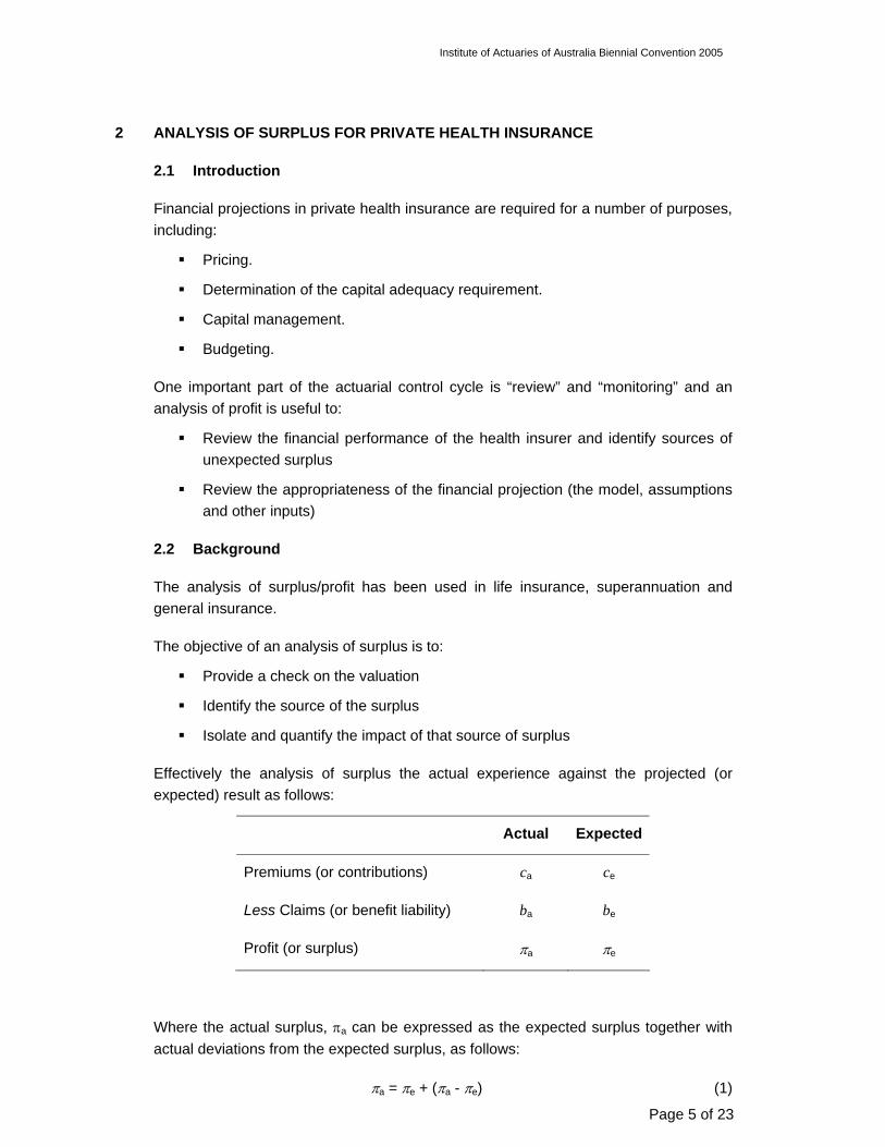
Effectively the analysis of surplus the actual experience against the projected (or expected) result as follows:

Actual Expected

Premiums (or contributions) ca ce

Less Claims (or benefit liability) ba be

Profit (or surplus) πa πe

Where the actual surplus, πa can be expressed as the expected surplus together with actual deviations from the expected surplus, as follows:

πa = πe + (πa - πe) (1)


of 23

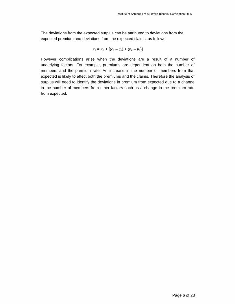
The deviations from the expected surplus can be attributed to deviations from the expected premium and deviations from the expected claims, as follows:

πa = πe + [(ca – ce) + (be – ba)]

However complications arise when the deviations are a result of a number of underlying factors. For example, premiums are dependent on both the number of members and the premium rate. An increase in the number of members from that expected is likely to affect both the premiums and the claims. Therefore the analysis of surplus will need to identify the deviations in premium from expected due to a change in the number of members from other factors such as a change in the premium rate from expected.


of 23

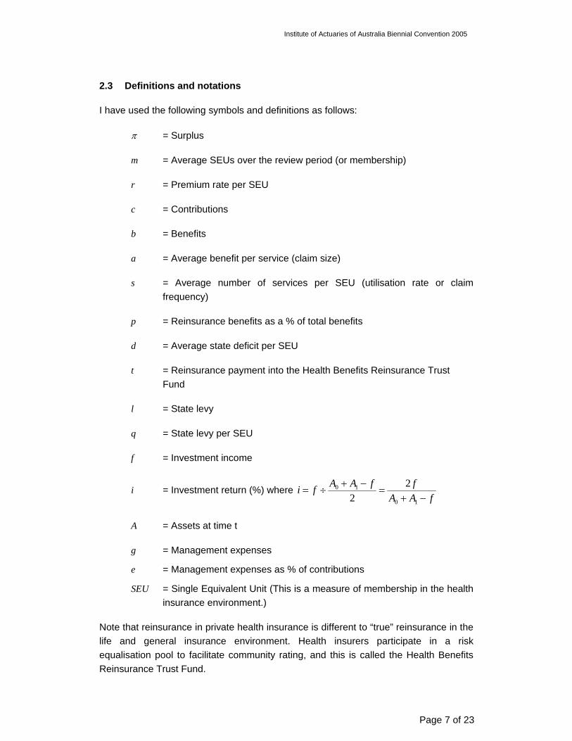
2.3 Definitions and notations

I have used the following symbols and definitions as follows:

π = Surplus

m = Average SEUs over the review period (or membership)

r = Premium rate per SEU

c = Contributions

b = Benefits

a = Average benefit per service (claim size)

s = Average number of services per SEU (utilisation rate or claim frequency)

p = Reinsurance benefits as a % of total benefits

d = Average state deficit per SEU

t = Reinsurance payment into the Health Benefits Reinsurance Trust Fund

l = State levy

q = State levy per SEU

f = Investment income

i = Investment return (%) where fAA

ffAAfi−+

=−+

÷=10

10 22

A = Assets at time t

g = Management expenses

e = Management expenses as % of contributions

SEU = Single Equivalent Unit (This is a measure of membership in the health insurance environment.)

Note that reinsurance in private health insurance is different to “true” reinsurance in the life and general insurance environment. Health insurers participate in a risk equalisation pool to facilitate community rating, and this is called the Health Benefits Reinsurance Trust Fund.


of 23

2.4 Assumptions

Several assumptions have been made to simplify this paper, as follows:

Only 1 hospital product.

The number of services eligible for reinsurance is based on the proportion of reinsurance benefits as a percentage of total benefits.

Contributions have no discounts or rate protection provisions.

Total assets are used to determine of investment income and other income.

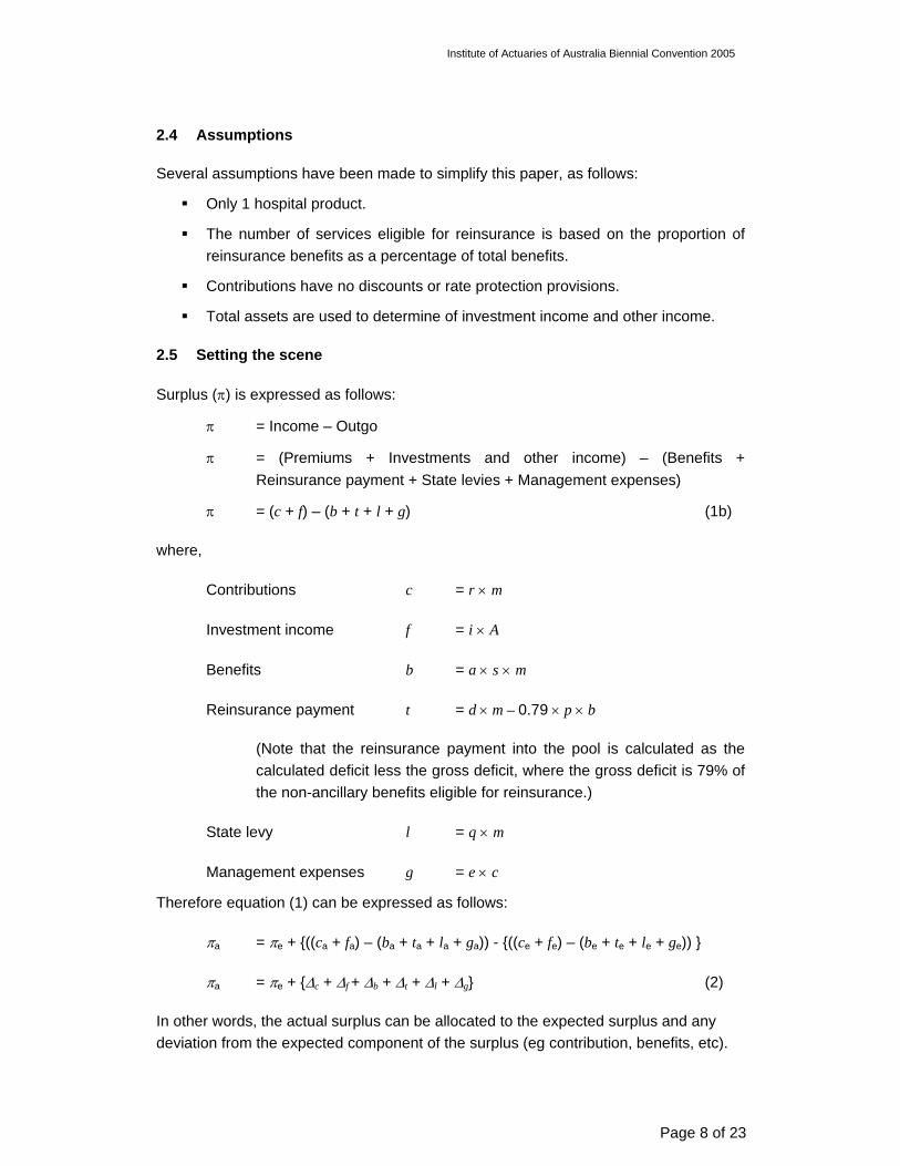
2.5 Setting the scene

Surplus (π) is expressed as follows:

π = Income – Outgo

π = (Premiums + Investments and other income) – (Benefits + Reinsurance payment + State levies + Management expenses)

π = (c + f) – (b + t + l + g) (1b)

where,

Contributions c = r × m

Investment income f = i × A

Benefits b = a × s × m

Reinsurance payment t = d × m – 0.79 × p × b

(Note that the reinsurance payment into the pool is calculated as the calculated deficit less the gross deficit, where the gross deficit is 79% of the non-ancillary benefits eligible for reinsurance.)

State levy l = q × m

Management expenses g = e × c

Therefore equation (1) can be expressed as follows:

πa = πe + {((ca + fa) – (ba + ta + la + ga)) - {((ce + fe) – (be + te + le + ge)) }

πa = πe + {∆c + ∆f + ∆b + ∆t + ∆l + ∆g} (2)

In other words, the actual surplus can be allocated to the expected surplus and any deviation from the expected component of the surplus (eg contribution, benefits, etc).


of 23

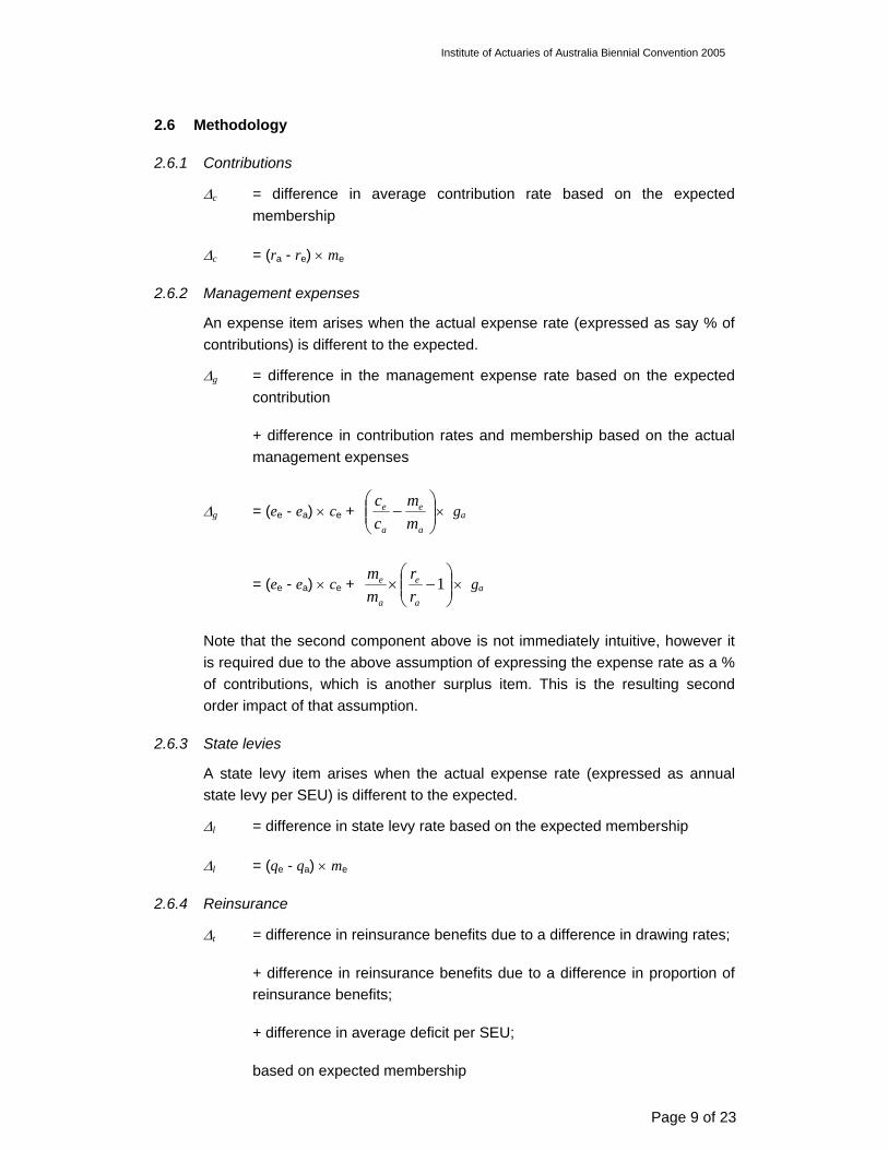
2.6 Methodology

2.6.1 Contributions

∆c = difference in average contribution rate based on the expected membership

∆c = (ra - re) × me

2.6.2 Management expenses

An expense item arises when the actual expense rate (expressed as say % of contributions) is different to the expected.

∆g = difference in the management expense rate based on the expected contribution

+ difference in contribution rates and membership based on the actual management expenses

∆g = (ee - ea) × ce + ⎟⎟⎠

⎞⎜⎜⎝

⎛−

a

e

a

e

mm

cc

× ga

= (ee - ea) × ce + ⎟⎟⎠

⎞⎜⎜⎝

⎛−× 1

a

e

a

e

rr

mm

× ga

Note that the second component above is not immediately intuitive, however it is required due to the above assumption of expressing the expense rate as a % of contributions, which is another surplus item. This is the resulting second order impact of that assumption.

2.6.3 State levies

A state levy item arises when the actual expense rate (expressed as annual state levy per SEU) is different to the expected.

∆l = difference in state levy rate based on the expected membership

∆l = (qe - qa) × me

2.6.4 Reinsurance

∆t = difference in reinsurance benefits due to a difference in drawing rates;

+ difference in reinsurance benefits due to a difference in proportion of reinsurance benefits;

+ difference in average deficit per SEU;

based on expected membership


of 23

∆t = (aa × sa – ae × se) × me × pa × 0.79 + (pa – pe) × be × 0.79 + (de – da) × me

2.6.5 Benefits

∆b = difference in drawing rates based on expected membership

∆b = (ae × se – aa × sa) × me

However, a more insightful analysis is to split the drawing rate into average benefits and utilisation, as follows:

∆b = difference in average benefits + difference in utilisation

Let

AP = (aa– ae) × se / {(sa– se) × ae + (aa– ae) × se }

UP = (sa– se) × ae / {(sa– se) × ae + (aa– ae) × se }

Where AP + UP = 1

∆b’ = ∆b × AP + ∆b × UP

2.6.6 Membership movements

∆m = impact of difference in SEUs (or membership)

∆m = difference in SEUs × actual surplus per SEUs

∆m = (ma - me) × πa / ma

2.6.7 Investment income

∆f = fa - fe = ia × Aa – ie × Ae

which can be re-arranged to

∆f = difference in investment rate + difference in assets (due to accumulated surplus)

∆f = (ia - ie) × Ae + (Aa - Ae) × ia

Note that2

10 eeee

fAAA −+= and

210 aaa

afAAA −+

=

(Aa - Ae) × ia can be re-expressed as 2ai × (πa - πe - (fa - fe)) given that the asset

movement is caused by gross of investment income surplus.

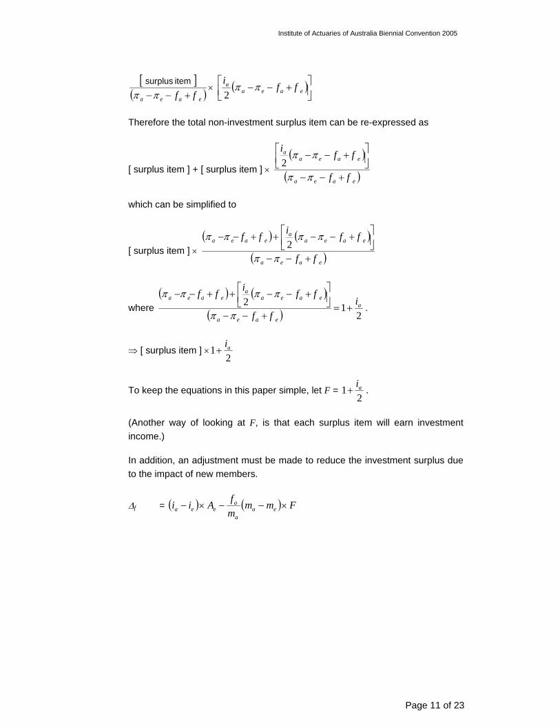
This can be re-allocated back to the non-investment surplus item as follows:


of 23

[ ]( )eaea ff +−−ππ

item surplus × ( )⎥⎦

⎤⎢⎣⎡ +−− eaea

a ffi ππ2

Therefore the total non-investment surplus item can be re-expressed as

[ surplus item ] + [ surplus item ] × ( )

( )eaea

eaeaa

ff

ffi

+−−

⎥⎦⎤

⎢⎣⎡ +−−

ππ

ππ2

which can be simplified to

[ surplus item ] × ( ) ( )

( )eaea

eaeaa

eaea

ff

ffiff

+−−

⎥⎦⎤

⎢⎣⎡ +−−++−−

ππ

ππππ2

where ( ) ( )

( ) 212 a

eaea

eaeaa

eaea iff

ffiff+=

+−−

⎥⎦⎤

⎢⎣⎡ +−−++−−

ππ

ππππ.

⇒ [ surplus item ] ×2

1 ai+

To keep the equations in this paper simple, let F = 2

1 ai+ .

(Another way of looking at F, is that each surplus item will earn investment income.)

In addition, an adjustment must be made to reduce the investment surplus due to the impact of new members.

∆f = ( ) ( ) FmmmfAii ea

a

aeea ×−−×−


of 23

2.7 Summary

In summary, equation (1) can be expressed as equation (2) given equation (1b) as follows:

πa = πe + (πa - πe) (1)

Given π = (c + f) – (b + t + l + g) (1b)

πa = πe + {∆c + ∆f + ∆b + ∆t + ∆l + ∆g} (2)

where

∆g = (ee - ea) × ce × F + ⎟⎟⎠

⎞⎜⎜⎝

⎛−× 1

a

e

a

e

rr

mm

× ga × F

∆l = (qe - qa) × me × F

∆t = { (aa × sa – ae × se) × me × pa × 0.79 + (pa – pe) × be × 0.79 + (de – da) × me }× F

∆c = (ra - re) × me × F

∆b(avg benefit) = (ae × se – aa × sa) × me × F × AP

∆b(util rate) = (ae × se – aa × sa) × me × F × UP

AP = (aa– ae) × se / {(sa– se) × ae + (aa– ae) × se }

UP = 1 - AP

∆m = (ma - me) × πa / ma × F

∆f = ( ) ( ) FmmmfAii ea

a

aeea ×−−×−

Where F = 2

1 ai+


of 23

3 A PRACTICAL EXAMPLE

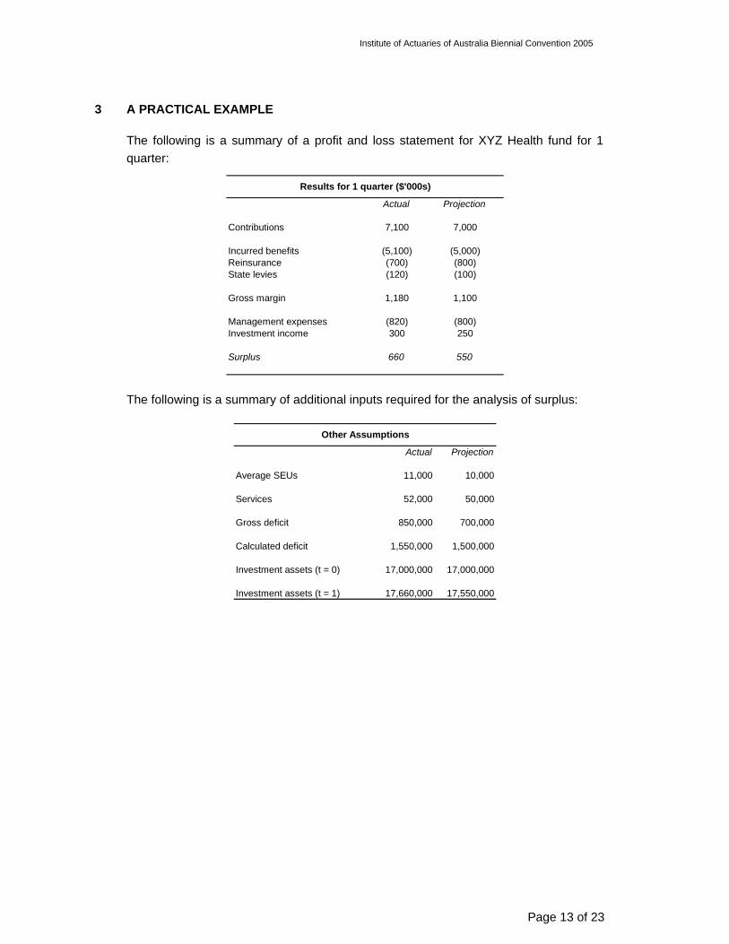
The following is a summary of a profit and loss statement for XYZ Health fund for 1 quarter:

Actual Projection

Contributions 7,100 7,000

Incurred benefits (5,100) (5,000)Reinsurance (700) (800)State levies (120) (100)

Gross margin 1,180 1,100

Management expenses (820) (800)Investment income 300 250

Surplus 660 550

Results for 1 quarter ($'000s)

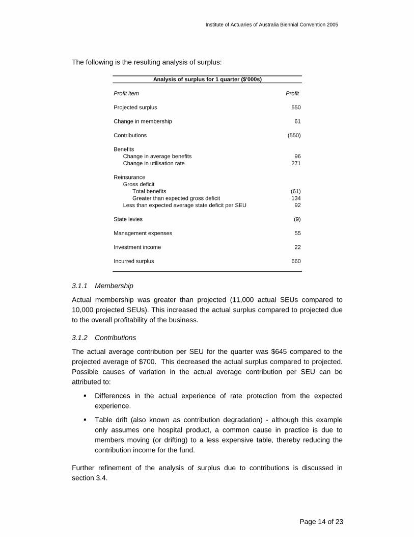
The following is a summary of additional inputs required for the analysis of surplus:

Actual Projection

Average SEUs 11,000 10,000

Services 52,000 50,000

Gross deficit 850,000 700,000

Calculated deficit 1,550,000 1,500,000

Investment assets (t = 0) 17,000,000 17,000,000

Investment assets (t = 1) 17,660,000 17,550,000

Other Assumptions


of 23

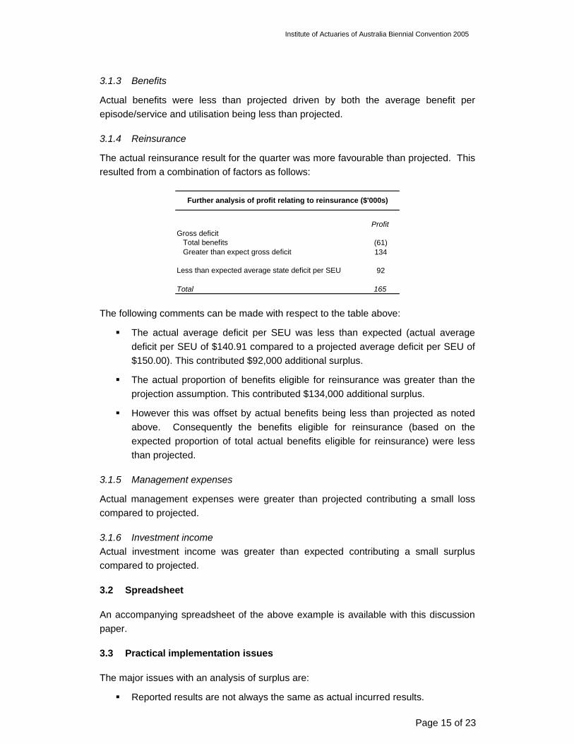
The following is the resulting analysis of surplus:

Profit item Profit

Projected surplus 550

Change in membership 61

Contributions (550)

BenefitsChange in average benefits 96Change in utilisation rate 271

ReinsuranceGross deficit

Total benefits (61)Greater than expected gross deficit 134

Less than expected average state deficit per SEU 92

State levies (9)

Management expenses 55

Investment income 22

Incurred surplus 660

Analysis of surplus for 1 quarter ($'000s)

3.1.1 Membership

Actual membership was greater than projected (11,000 actual SEUs compared to 10,000 projected SEUs). This increased the actual surplus compared to projected due to the overall profitability of the business.

3.1.2 Contributions

The actual average contribution per SEU for the quarter was $645 compared to the projected average of $700. This decreased the actual surplus compared to projected. Possible causes of variation in the actual average contribution per SEU can be attributed to:

Differences in the actual experience of rate protection from the expected experience.

Table drift (also known as contribution degradation) - although this example only assumes one hospital product, a common cause in practice is due to members moving (or drifting) to a less expensive table, thereby reducing the contribution income for the fund.

Further refinement of the analysis of surplus due to contributions is discussed in section 3.4.


of 23

3.1.3 Benefits

Actual benefits were less than projected driven by both the average benefit per episode/service and utilisation being less than projected.

3.1.4 Reinsurance

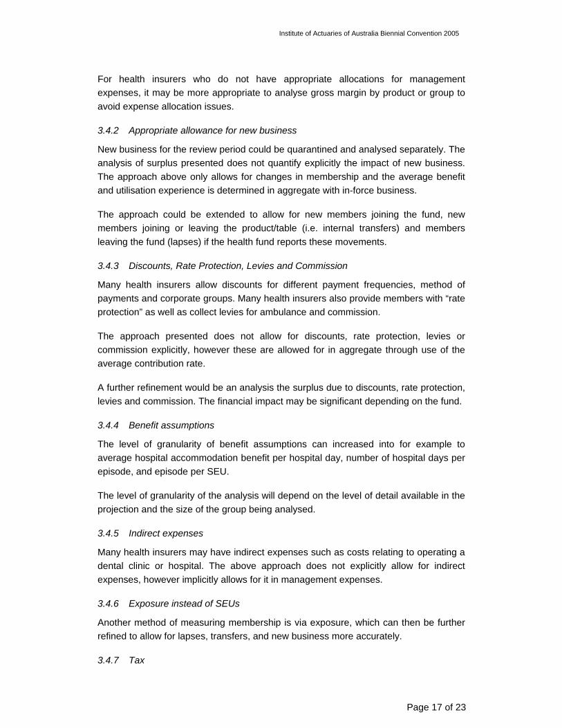
The actual reinsurance result for the quarter was more favourable than projected. This resulted from a combination of factors as follows:

ProfitGross deficit

Total benefits (61)Greater than expect gross deficit 134

Less than expected average state deficit per SEU 92

Total 165

Further analysis of profit relating to reinsurance ($'000s)

The following comments can be made with respect to the table above:

The actual average deficit per SEU was less than expected (actual average deficit per SEU of $140.91 compared to a projected average deficit per SEU of $150.00). This contributed $92,000 additional surplus.

The actual proportion of benefits eligible for reinsurance was greater than the projection assumption. This contributed $134,000 additional surplus.

However this was offset by actual benefits being less than projected as noted above. Consequently the benefits eligible for reinsurance (based on the expected proportion of total actual benefits eligible for reinsurance) were less than projected.

3.1.5 Management expenses

Actual management expenses were greater than projected contributing a small loss compared to projected.

3.1.6 Investment income Actual investment income was greater than expected contributing a small surplus compared to projected.

3.2 Spreadsheet

An accompanying spreadsheet of the above example is available with this discussion paper.

3.3 Practical implementation issues

The major issues with an analysis of surplus are:

Reported results are not always the same as actual incurred results.


of 23

A check on the provision of outstanding claims is required to ensure that the actual reported results reasonably reflect the actual incurred results.

The state average deficit per SEU is notoriously difficult to project.

Due to delays between the date of service and the date of processing, an estimate of the outstanding claims is required to determine the ultimate incurred benefits.

Over time as actual claims are received (or developed), the level of the outstanding claims reduces and the confidence in the estimate of the ultimate incurred benefit increases.

The delay period and pattern of claim development depend on the claim type:

Most hospital claims typically have a delay of up to 3 months.

Medical claims usually have a similar delay development to hospital claims, however this can differ as medical claims are not processed by the hospital.

Ancillary claims which are on HICAPs will have no delay. HICAPs is an electronic payment system, which enables the health insurer to pay the service provider without delay.

Ancillary claims which are not on HICAPs may have a delay of up to several months.

For most health insurers, the majority of claims are received/paid within 3 months of the original date of service.

This implies that an analysis of surplus can be performed on the “time underlying result” approximately 3 months after results are reported.

The appropriateness of the provision of outstanding claims depends on the methodology and assumptions adopted. The accuracy of the reported results may be impacted by changes in the provision for outstanding claims.

Similarly, reported results can include estimates for reinsurance transfers which may differ from the actual transfer.

The review of the outstanding claims provision is further discussed in section 4.

3.4 Further development

The analysis of surplus presented is one example and can be further refined. The following are a few suggested modifications.

3.4.1 By product, benefit type, scale, group, state etc.

To provide management with further insights on profitability, the analysis of surplus can be performed on products or tables, benefit types, business lines, scales, groups, states, segments, etc. The level of granularity will however depend on the level of detail available in the projection and underlying assumptions.


of 23

For health insurers who do not have appropriate allocations for management expenses, it may be more appropriate to analyse gross margin by product or group to avoid expense allocation issues.

3.4.2 Appropriate allowance for new business

New business for the review period could be quarantined and analysed separately. The analysis of surplus presented does not quantify explicitly the impact of new business. The approach above only allows for changes in membership and the average benefit and utilisation experience is determined in aggregate with in-force business.

The approach could be extended to allow for new members joining the fund, new members joining or leaving the product/table (i.e. internal transfers) and members leaving the fund (lapses) if the health fund reports these movements.

3.4.3 Discounts, Rate Protection, Levies and Commission

Many health insurers allow discounts for different payment frequencies, method of payments and corporate groups. Many health insurers also provide members with “rate protection” as well as collect levies for ambulance and commission.

The approach presented does not allow for discounts, rate protection, levies or commission explicitly, however these are allowed for in aggregate through use of the average contribution rate.

A further refinement would be an analysis the surplus due to discounts, rate protection, levies and commission. The financial impact may be significant depending on the fund.

3.4.4 Benefit assumptions

The level of granularity of benefit assumptions can increased into for example to average hospital accommodation benefit per hospital day, number of hospital days per episode, and episode per SEU.

The level of granularity of the analysis will depend on the level of detail available in the projection and the size of the group being analysed.

3.4.5 Indirect expenses

Many health insurers may have indirect expenses such as costs relating to operating a dental clinic or hospital. The above approach does not explicitly allow for indirect expenses, however implicitly allows for it in management expenses.

3.4.6 Exposure instead of SEUs

Another method of measuring membership is via exposure, which can then be further refined to allow for lapses, transfers, and new business more accurately.

3.4.7 Tax


of 23

The current approach does not allow for taxation of surplus. Another refinement could be the inclusion of tax in the analysis of surplus.

3.4.8 Other

The approach presented can also be refined to allow for changes in modelling methodology, assumption changes, asset valuation techniques and changes in the method of determining the provision for outstanding claims.

3.5 Timing of review

The frequency of performing an analysis of surplus would vary from health fund to health fund. An analysis of surplus should be performed at least once a year however best practice suggests an analysis of surplus each quarter.

The timeframe of the analysis may change depending on how frequently the health insurer’s financial projections are revised.

3.6 Materiality

While it may be theoretically possible and actuarially sound to “drill-down” to a very focused level, the results may become spurious, and will be driven by the amount of data available.

3.7 Conclusion

An analysis of surplus is an invaluable tool to manage the appropriateness of financial projections for various purposes.

Further refinement will depend on the level of detail available in supporting assumptions and therefore the projection results. Practical restrictions may limit the resolution of the analysis.


of 23

4 REVIEW OF THE PROVISION OF OUTSTANDING CLAIMS

4.1 Introduction

Section 2.10 of the Health Benefits Organizations - Interpretation Standard 2003 defines the outstanding claims liability as follows:

“Outstanding Claims Liability is the best estimate liability in respect of the accrued but not admitted claims, and related expense, liabilities of the Fund at the valuation date.” And,

“Outstanding claims relate to claims that have been reported and have not yet been settled, claims which have been incurred but not yet reported (IBNR) and claims which have been administratively finalised and which may be reopened.”

The outstanding claims liability in this discussion paper will be referred to as the provision for outstanding claims to remind the reader that it is an estimate of the actual outstanding claims.

The movement in the provision over a period plus the benefits paid to contributors during that period provides an estimate of the actual incurred claims for the period.

The majority of health insurers are not-for-profit organisations and tend to have a relatively smaller surplus than for-profit organisations. Health insurers with a long delay between date of service and date of payment may result in a large provision for outstanding claims. As such, the movement in a large provision for outstanding claims can potentially be a significant driver of the surplus, therefore having a hyper-sensitive impact on the surplus.

4.2 Objectives of this section

This section of the discussion paper aims to focus on managing the sufficiency of the provision, particularly the gross component of the provision.

4.3 Background

The provision is composed of the following components:

Gross component – this refers to unpresented and outstanding claims gross of reinsurance recoveries from and payments to the Reinsurance Trust Fund.

Administration component – this refers to any administration expenses that may be incurred by these outstanding claims.

Reinsurance component – this refers to the net amount in respect of recoveries from and payments to the Reinsurance Trust Fund in respect of unpresented and outstanding claims.


of 23

This section focuses on the gross component and any reference to the estimate of the provision of outstanding claims refers to the gross component as the administration component and reinsurance component are likely to be relatively small.

4.4 Determination of the provision for outstanding claims

The following is a brief summary of methods encountered in the current private health insurance environment to determine the outstanding claims provision:

Paid chain-ladder method as per the PHIAC 2 template.

Modified chain-ladder method. This is the paid chain-ladder method with manual adjustments (for judgement, additional information from claims management, etc).

Chain ladder modified by statistical analysis.

Provisions may be determined separately by:

Benefit type (e.g. hospital, medical, dental, ancillary, etc)

Product

State

The approach adopted will vary with the amount of credible data and internal reporting requirements.

The outstanding claims provision should be reviewed regularly to ensure:

The determination of for the provision is appropriate, i.e. the provision provides a reasonable estimate of the actual outstanding claims.

The provision is not biased, i.e. the estimate does not regularly over or under estimate the estimate.

The volatility of the estimate around the actual does not increase over time, i.e. the absolute difference between the estimate and the actual outstanding claims does not increase over time.

4.5 Sufficiency of the provision

A need for a review of sufficiency is required to ensure that the determination of the provision is suitable and appropriate.

The following different “actual Vs expected” reviews have been observed:

A comparison of:

o The initial estimate of the gross provision for outstanding claims at a point in time, say 30 June 2004; against

o Actual claims paid to say, 30 September 2004, in respect of claims incurred up to 30 June 2004. This assumes that the majority of outstanding claims are processed within 3 months of the incurred date.


of 23

A comparison of the initial provision for outstanding claims is made against each succeeding month’s revision of the provision.

For each incurred month, a comparison of the initial estimate of incurred claims against each succeeding month’s revision of the incurred claims.

A comparison of the estimated incurred claims and incurred drawing rates against historical trends of incurred claims over time.

The first review method described above is perhaps the least complicated, however it has the following disadvantages:

It assumes that a high proportion of claims are paid within 3 months. Some health insurers may have delays of more or less than 3 months.

Health insurers will need to wait 3 months before a review can be performed.

The second review method is similar to the first except it is performed earlier and more regularly. This is useful check for health insurers that perform monthly reporting to ensure sufficiency of the estimate from the previous month.

The third review method is essentially the same as the first two methods above except that the comparison is made against incurred claims as opposed to outstanding claims.

The final review method above is a complimentary check that some health insurers have used to check that the estimated incurred claims is consistent with historical trends of incurred claims on a monthly basis.

4.6 Bias

The estimate of the provision should not be biased i.e. the estimate of the provision should be greater than the actual amount 50% of the time and less than the actual amount 50% of the time. If the estimate of the provision is continually greater or less than the actual amount, then the estimate could be said to be biased.

Solely measuring an absolute tolerance level does not appropriately measure bias.

A measure of the bias could be the measurement of cumulative tolerance (plus and minus) on a rolling 12-month basis. Over time this should be close to zero.

4.7 Variability

The volatility of the estimate of the provision around the actual should be as small as possible and not increase over time. This can be determined by measuring the standard deviation over time to determine its size and trend.

The standard deviation over time should be monitored to ensure that:


of 23

The standard deviation is not too high (i.e. the estimates are reasonably close);

The volatility of the estimate is not increasing over time.

Measuring the tolerance on a monthly basis may be inappropriate due to the volatility of the monthly results. A more appropriate measurement may be a rolling 12, 18 or 24 months.

4.8 The provision of outstanding claims for the annual report

For the purpose of annual results (to 30 June), it appears common practice in the industry to revise the provision for outstanding claims with actual claims paid to late September in respect of the incurred period (12 months to 30 June).

As

A significant proportion of hospital and medical claims are usually paid within 3 months of the date of service; and

A significant proportion of ancillary claims are paid via HICAPS which minimises the delay between the date of service and date of payment of the benefit.

the revised estimate can be expected to have a low level of uncertainty with the “outstanding claims” relating to longer-tail (greater than 3 months delayed) claims.

This approach raises some interesting issues with respect to risk margins that will be required under IFRS.

4.9 Conclusion

Health funds need to assess the sufficiency of their outstanding claims provision as part of the “review” and “monitor” components of the actuarial control cycle to address the following:

Assessment of sufficiency of past provisions, including bias and variability of the past provisions;

Assessment of the approach used in determining the provision;

Scope for improvement in future provision determination.


of 23

5 ACKNOWLEDGEMENTS

I would like to thank Barry Leung and my colleagues at KPMG Actuaries and in particular, David Torrance and Dimity Wall for the onerous task of peer reviewing this paper and supporting spreadsheet. I am grateful for their helpful comments and suggestions.

6 REFERENCES

Goford J, (1985) The Control Cycle: Financial control of a life assurance company, TIAA 1985.

Health Benefits Organizations — Solvency Standard 2003, PHIAC 2003

Health Benefits Organizations — Capital Adequacy Standard 2003, PHIAC 2003

Health Benefits Organizations — Intepretations Standard 2003, PHIAC 2003

Applying the actuarial control cycle in private health ... Paper_Control... · One important part...

Documents

Transcript of Applying the actuarial control cycle in private health ... Paper_Control... · One important part...