Applications of The Normal Laplace and Generalized Normal ...

Applications of The Normal Laplace and

Generalized Normal Laplace Distributions

by

Fan WuBA. (Honors) University of Western Ontario 2005

M.Sc. University of Victoria 2008

A Thesis Submitted in Partial Fullfillment of theRequirements for the Degree of

MASTER OF SCIENCE

in the Department of Mathematics and Statistics

c© Fan Wu, 2008University of Victoria

All rights reserved. This thesis may not be reproduced in whole or in part, byphotocopy or other means, without the permission of the author.

ii

Applications of The Normal Laplace and

Generalized Normal Laplace Distributions

by

Fan WuBA. (Honors) University of Western Ontario 2005

M.Sc. University of Victoria 2008

Supervisory Committee

Dr. William J. Reed (Department of Mathematics and Statistics)Supervisor

Dr. Julie Zhou (Department of Mathematics and Statistics)Departmental Member

Dr. Farouk Nathoo (Department of Mathematics and Statistics)Departmental Member

Dr. Judith A. Clarke (Department of Economics)External Examiner

iii

Supervisory Committee

Dr. William J. Reed (Department of Mathematics and Statistics)Supervisor

Dr. Julie Zhou (Department of Mathematics and Statistics)Departmental Member

Dr. Farouk Nathoo (Department of Mathematics and Statistics)Departmental Member

Dr. Judith A. Clarke (Department of Economics)External Examiner

Abstract

Two parametric models for income and financial return distributions are pre-

sented. There are the four-parameter normal Laplace (NL) and the five-parameter

generalized normal Laplace (GNL) distributions. Their properties are discussed;

furthermore, estimation of the parameters by the method of moments and maximum

likelihood is presented. The performances of fitting the two models to nine empirical

distributions of family income have been evaluated and compared against the four-

and five-parameter generalized beta2 (GB2) and generalized beta (GB) distributions

which had been previously claimed as best-fitting four- and five- parameter models

for income distribution. The results demonstrate that the NL distribution has better

performance than the GB and GB2 distributions with the GNL distribution providing

an even better fit. Limited application to data on financial log returns shows that the

fit of the GNL is comparable to the well-known generalized hyperbolic distribution.

However, the GNL suffers from a lack of closed-form expressions for its probability

density and cumulative distribution functions, and fitting the distribution numeri-

cally is slow and not always reliable. The results of this thesis suggest a strong case

for considering the GNL family as parametric models for income data and possibly

for financial logarithmic returns.

iv

Table of Contents

Supervisory committee . . . . . . . . . . . . . . . . . . . . . . . . . . . . . . . ii

Abstract . . . . . . . . . . . . . . . . . . . . . . . . . . . . . . . . . . . . . . . iii

Table of Contents . . . . . . . . . . . . . . . . . . . . . . . . . . . . . . . . . . iv

List of Figures . . . . . . . . . . . . . . . . . . . . . . . . . . . . . . . . . . . vi

Acknowledgments . . . . . . . . . . . . . . . . . . . . . . . . . . . . . . . . . . vii

List of abbreviations . . . . . . . . . . . . . . . . . . . . . . . . . . . . . . . . viii

1. Introduction . . . . . . . . . . . . . . . . . . . . . . . . . . . . . . . . . . . 1

1.1 Income Distributions . . . . . . . . . . . . . . . . . . . . . . . . . . . 2

1.2 Financial Return Distributions . . . . . . . . . . . . . . . . . . . . . . 4

1.2.1 Generalized Hyperbolic Distribution . . . . . . . . . . . . . . 6

2. The Normal-Laplace and Generalized Normal Laplace Distributions . . . . 8

2.1 The Laplace Distribution . . . . . . . . . . . . . . . . . . . . . . . . . 8

2.2 Normal Laplace Distribution . . . . . . . . . . . . . . . . . . . . . . . 9

2.2.1 Properties . . . . . . . . . . . . . . . . . . . . . . . . . . . . . 10

2.3 Generalized Laplace Distribution . . . . . . . . . . . . . . . . . . . . 11

2.4 Generalized Normal Laplace (GNL) Distribution . . . . . . . . . . . . 13

2.5 Properties of the GNL Distribution . . . . . . . . . . . . . . . . . . . 18

2.5.1 Infinite Divisibility . . . . . . . . . . . . . . . . . . . . . . . . 18

2.5.2 Mean, Variance and Cumulants . . . . . . . . . . . . . . . . . 19

2.6 Numerical determination of the pdf and cdf of the GNL . . . . . . . . 22

2.6.1 Using the Representation as a Convolution . . . . . . . . . . . 23

2.6.2 Numerical Inversion of Characteristic Function . . . . . . . . . 24

2.6.3 Using the representation as a Normal mean-variance mixture . 25

v

3. Methods of Estimation . . . . . . . . . . . . . . . . . . . . . . . . . . . . . 27

3.1 Method of Moments . . . . . . . . . . . . . . . . . . . . . . . . . . . 27

3.2 Maximum Likelihood Estimation . . . . . . . . . . . . . . . . . . . . 30

3.3 Nelder-Mead Method: Multi-dimensional Maximization Method . . . 34

4. Simulation Studies for The GNL distribution . . . . . . . . . . . . . . . . . 36

4.1 Simulating GNL Data . . . . . . . . . . . . . . . . . . . . . . . . . . 36

4.2 Simulating GH Data . . . . . . . . . . . . . . . . . . . . . . . . . . . 40

5. Application to Income Data . . . . . . . . . . . . . . . . . . . . . . . . . . 43

5.1 Description of the Income Data . . . . . . . . . . . . . . . . . . . . . 43

5.2 Income Distribution Results . . . . . . . . . . . . . . . . . . . . . . . 46

6. Application To Financial Data . . . . . . . . . . . . . . . . . . . . . . . . . 50

6.1 Description of the Stock Price Data . . . . . . . . . . . . . . . . . . . 50

6.2 Results of fitting GNL and GH . . . . . . . . . . . . . . . . . . . . . 50

7. Conclusions . . . . . . . . . . . . . . . . . . . . . . . . . . . . . . . . . . . 53

References . . . . . . . . . . . . . . . . . . . . . . . . . . . . . . . . . . . . . . 55

Appendix . . . . . . . . . . . . . . . . . . . . . . . . . . . . . . . . . . . . . . 60

vi

List of Figures

2.1 The effect of the parameters of GL and the comparison of GL and normaldistributions. . . . . . . . . . . . . . . . . . . . . . . . . . . . . . . . . . 13

2.2 A comparison of the pdf curves of GNL(0,1,1,1, ρ) and N (0,1) distributions. 14

2.3 The pdf curves of three GNL distributions (effect of µ) . . . . . . . . . 15

2.4 The pdf curves of three GNL distributions (effect of σ) . . . . . . . . . 16

2.5 The pdf curves of three GNL distributions (effect of α) . . . . . . . . . 17

2.6 The pdf curves of three GNL distributions (effect of β) . . . . . . . . . 17

2.7 The pdf curves of four GNL distributions (effect of ρ) . . . . . . . . . . 18

2.8 The pdf curves and means of three GNL distributions (effect of α onmean) . . . . . . . . . . . . . . . . . . . . . . . . . . . . . . . . . . . . 20

2.9 The pdf curves and means of three GNL distributions (effect of β onmean) . . . . . . . . . . . . . . . . . . . . . . . . . . . . . . . . . . . . 21

4.1 Q-Q plots for the simulated GNL data . . . . . . . . . . . . . . . . . . . 38

4.2 Q-Q plots for the simulated GNL data . . . . . . . . . . . . . . . . . . . 39

4.3 Q-Q plot for the GNL . . . . . . . . . . . . . . . . . . . . . . . . . . . . 41

4.4 Q-Q plot for the GH . . . . . . . . . . . . . . . . . . . . . . . . . . . . 42

6.1 The GNL fitted to IBM 05-06 . . . . . . . . . . . . . . . . . . . . . . . 51

6.2 The GH fitted to IBM 05-06 . . . . . . . . . . . . . . . . . . . . . . . . 51

6.3 The GNL fitted to CitiGroup 05-06 . . . . . . . . . . . . . . . . . . . . 52

6.4 The GH fitted to CitiGroup 05-06 . . . . . . . . . . . . . . . . . . . . . 52

vii

Acknowledgments

I would first like to thank my father Wu, Shaoqin, mother Chen, Yuhua and all

my family members. Without their support, I could not have got to the point of

writing this thesis. Dr. William J. Reed has guided me in the fields of statistics and

finance, and provided many ideas, and offered infinite help and patience during my

study at the University of Victoria. I owe him a lot. I would like to acknowledge my

gratitude to my committee members, Dr. Julie Zhou and Dr. Farouk Nathoo who

have been very helpful in assisting in the completion of the thesis. I would also like

to acknowledge LIS. Without their data, this thesis could not have been completed.

viii

List of abbreviations

cdf...............................Cumulative Distribution Function (1)

cgf...............................Cumulant Generating Function (2)

ch.f..............................Characteristic Function (3)

pdf...............................Probability Distribution Function (4)

Dist’n..........................Distribution (5)

GL..............................Generalized Laplace (6)

GNL...........................Generalized Normal Laplace (7)

GB2............................Generalized Beta 2 (8)

GB..............................Generalized Beta (9)

GH..............................Generalized Hyperbolic (10)

GBM...........................Geometric Brownian Motion (11)

LIS...............................Luxembourg Income Study (12)

MLE............................Maximum Likelihood Estimation (13)

MME...........................Method of Moments Estimation (14)

NL...............................Normal Laplace (15)

Q-Q plot......................Quantile-quantile plot (16)

SSE..............................Sum of Squared Errors (17)

SAE.............................Sum of Absolute Errors (18)

Chapter 1

Introduction

A major aim of this thesis is to examine the performance of two new parametric

probability distributions, the normal Laplace (NL) and generalized normal Laplace

(GNL), in applications in economics and finance. In economics we consider fitting the

four-parameter NL distribution and the five-parameter GNL distribution to data on

income and earnings distributions. Reed and Jorgensen (2004) presented a number of

examples of the fit of the NL distribution to various empirical size distributions and

Reed (2004) gave examples of its fit to income distributions for four widely differing

data sets. However to date no comparison of the fit of the NL (or GNL) with other

proposed models has been conducted. In this thesis we perform such a comparison

using nine different empirical income distributions. In the finance field we consider

fitting the GNL distribution to logarithmic returns on financial assets. Reed (2004)

has shown how a Levy process, which he called Brownian-Laplace Motion whose

increments follow the GNL distribution can be constructed and used for modelling

stock-price dynamics; he obtained an option pricing formula for assets following such

a process. The GNL distribution can exhibit skewness and excess kurtosis, proper-

ties present in high-frequency data of logarithmic returns. It therefore seems a good

candidate model for use in option pricing. An aim of this thesis is to explore how

well it fits to actual stock-price data, and to compare it with other proposed models.

2

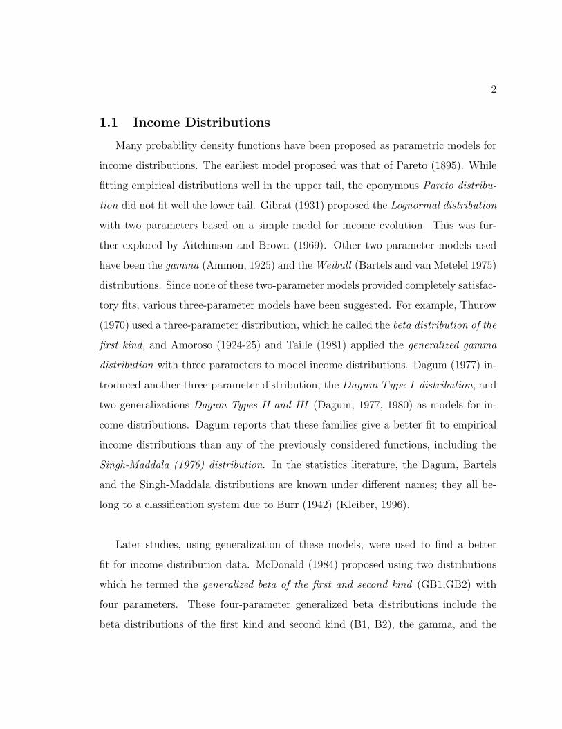
1.1 Income Distributions

Many probability density functions have been proposed as parametric models for

income distributions. The earliest model proposed was that of Pareto (1895). While

fitting empirical distributions well in the upper tail, the eponymous Pareto distribu-

tion did not fit well the lower tail. Gibrat (1931) proposed the Lognormal distribution

with two parameters based on a simple model for income evolution. This was fur-

ther explored by Aitchinson and Brown (1969). Other two parameter models used

have been the gamma (Ammon, 1925) and the Weibull (Bartels and van Metelel 1975)

distributions. Since none of these two-parameter models provided completely satisfac-

tory fits, various three-parameter models have been suggested. For example, Thurow

(1970) used a three-parameter distribution, which he called the beta distribution of the

first kind, and Amoroso (1924-25) and Taille (1981) applied the generalized gamma

distribution with three parameters to model income distributions. Dagum (1977) in-

troduced another three-parameter distribution, the Dagum Type I distribution, and

two generalizations Dagum Types II and III (Dagum, 1977, 1980) as models for in-

come distributions. Dagum reports that these families give a better fit to empirical

income distributions than any of the previously considered functions, including the

Singh-Maddala (1976) distribution. In the statistics literature, the Dagum, Bartels

and the Singh-Maddala distributions are known under different names; they all be-

long to a classification system due to Burr (1942) (Kleiber, 1996).

Later studies, using generalization of these models, were used to find a better

fit for income distribution data. McDonald (1984) proposed using two distributions

which he termed the generalized beta of the first and second kind (GB1,GB2) with

four parameters. These four-parameter generalized beta distributions include the

beta distributions of the first kind and second kind (B1, B2), the gamma, and the

3

lognormal as special cases, and proved to provide better fits than previous models.

The GB2 on the whole, provided a better fit than the GB1. (McDonald, 2002).

Subsequently, McDonald and Xu (1995) presented a new generalized five-parameter

distribution which they called the generalized beta (GB) distribution, which nests all

of the distributions that we have mentioned above as special cases. The GB is more

flexible and of course having all of the others nested within it provided a better fit

(McDonald 2002).

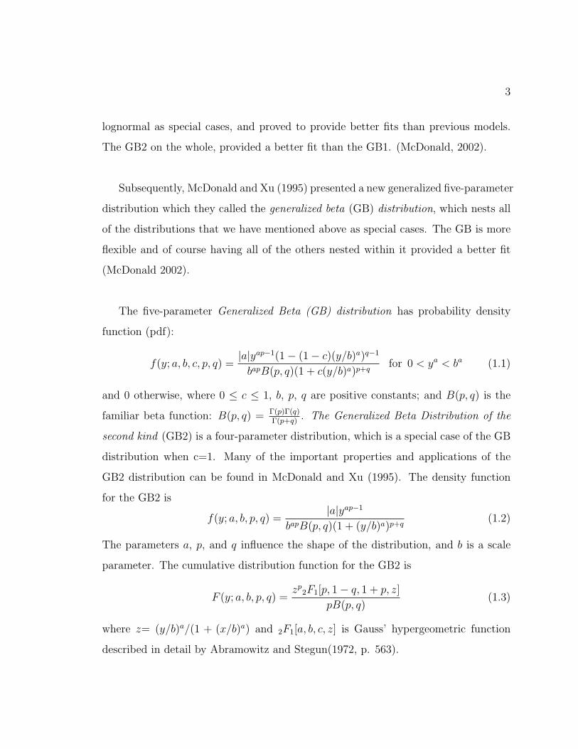
The five-parameter Generalized Beta (GB) distribution has probability density

function (pdf):

f(y; a, b, c, p, q) =|a|yap−1(1− (1− c)(y/b)a)q−1

bapB(p, q)(1 + c(y/b)a)p+qfor 0 < ya < ba (1.1)

and 0 otherwise, where 0 ≤ c ≤ 1, b, p, q are positive constants; and B(p, q) is the

familiar beta function: B(p, q) = Γ(p)Γ(q)Γ(p+q)

. The Generalized Beta Distribution of the

second kind (GB2) is a four-parameter distribution, which is a special case of the GB

distribution when c=1. Many of the important properties and applications of the

GB2 distribution can be found in McDonald and Xu (1995). The density function

for the GB2 is

f(y; a, b, p, q) =|a|yap−1

bapB(p, q)(1 + (y/b)a)p+q(1.2)

The parameters a, p, and q influence the shape of the distribution, and b is a scale

parameter. The cumulative distribution function for the GB2 is

F (y; a, b, p, q) =zp2F1[p, 1− q, 1 + p, z]

pB(p, q)(1.3)

where z= (y/b)a/(1 + (x/b)a) and 2F1[a, b, c, z] is Gauss’ hypergeometric function

described in detail by Abramowitz and Stegun(1972, p. 563).

4

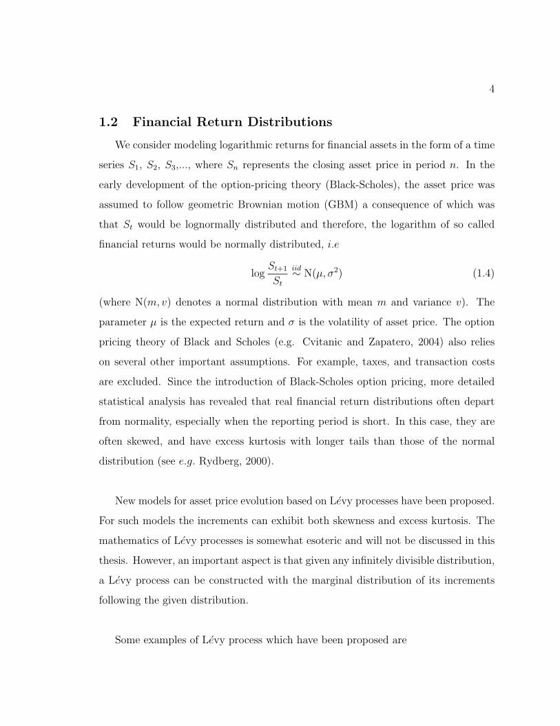
1.2 Financial Return Distributions

We consider modeling logarithmic returns for financial assets in the form of a time

series S1, S2, S3,..., where Sn represents the closing asset price in period n. In the

early development of the option-pricing theory (Black-Scholes), the asset price was

assumed to follow geometric Brownian motion (GBM) a consequence of which was

that St would be lognormally distributed and therefore, the logarithm of so called

financial returns would be normally distributed, i.e

logSt+1

St

iid∼ N(µ, σ2) (1.4)

(where N(m, v) denotes a normal distribution with mean m and variance v). The

parameter µ is the expected return and σ is the volatility of asset price. The option

pricing theory of Black and Scholes (e.g. Cvitanic and Zapatero, 2004) also relies

on several other important assumptions. For example, taxes, and transaction costs

are excluded. Since the introduction of Black-Scholes option pricing, more detailed

statistical analysis has revealed that real financial return distributions often depart

from normality, especially when the reporting period is short. In this case, they are

often skewed, and have excess kurtosis with longer tails than those of the normal

distribution (see e.g. Rydberg, 2000).

New models for asset price evolution based on Levy processes have been proposed.

For such models the increments can exhibit both skewness and excess kurtosis. The

mathematics of Levy processes is somewhat esoteric and will not be discussed in this

thesis. However, an important aspect is that given any infinitely divisible distribution,

a Levy process can be constructed with the marginal distribution of its increments

following the given distribution.

Some examples of Levy process which have been proposed are

5

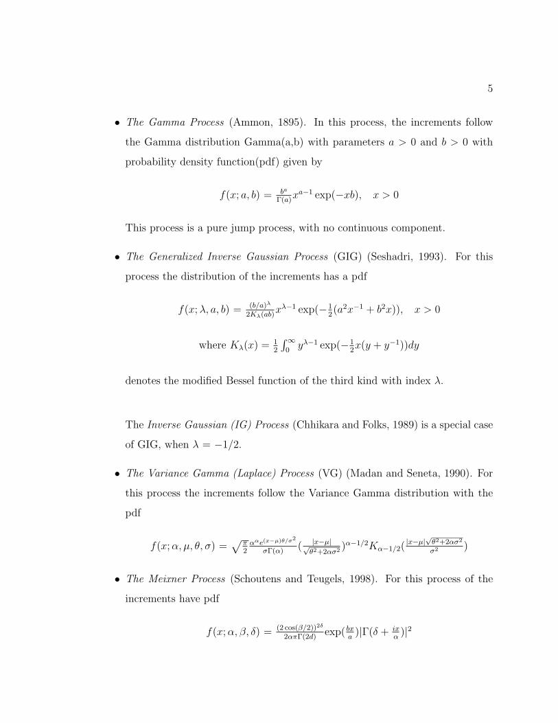
• The Gamma Process (Ammon, 1895). In this process, the increments follow

the Gamma distribution Gamma(a,b) with parameters a > 0 and b > 0 with

probability density function(pdf) given by

f(x; a, b) = ba

Γ(a)xa−1 exp(−xb), x > 0

This process is a pure jump process, with no continuous component.

• The Generalized Inverse Gaussian Process (GIG) (Seshadri, 1993). For this

process the distribution of the increments has a pdf

f(x;λ, a, b) = (b/a)λ

2Kλ(ab)xλ−1 exp(−1

2(a2x−1 + b2x)), x > 0

where Kλ(x) = 12

∫∞0yλ−1 exp(−1

2x(y + y−1))dy

denotes the modified Bessel function of the third kind with index λ.

The Inverse Gaussian (IG) Process (Chhikara and Folks, 1989) is a special case

of GIG, when λ = −1/2.

• The Variance Gamma (Laplace) Process (VG) (Madan and Seneta, 1990). For

this process the increments follow the Variance Gamma distribution with the

pdf

f(x;α, µ, θ, σ) =√

π2ααe(x−µ)θ/σ2

σΓ(α)( |x−µ|√

θ2+2ασ2 )α−1/2Kα−1/2( |x−µ|√θ2+2ασ2

σ2 )

• The Meixner Process (Schoutens and Teugels, 1998). For this process of the

increments have pdf

f(x;α, β, δ) = (2 cos(β/2))2δ

2απΓ(2d)exp( bx

a)|Γ(δ + ix

α)|2

6

• The CGMY Process (Carr, Geman, Madan and Yor, 2002). For this process

the distribution of the increments has a characteristic function of the form

φ(u;C,G,M, Y ) = exp(CΓ(−Y )((M − iu)Y −MY + (G+ iu)Y −GY ))

• The Generalized Hyperbolic Process (Eberlein and Hammerstein, 2002). For

this process the distribution of the increments has a pdf

f(x;λ, α, β, δ, µ) = a(λ, α, β, δ)(δ2 + (x− µ)2)(λ− 12

)/2

×Kλ− 12(α√δ2 + (x− µ)2) exp(β(x− µ)),

where

a(λ, α, β, δ) = (α2−β2)λ/2√

2παλ−12 δλKλ(δ

√α2−β2)

and Kλ the modified Bessel function of the third kind with index λ.

1.2.1 Generalized Hyperbolic Distribution

Barndorff-Nielsen (1977) introduced the four-parameter hyperbolic distribution,

which he fitted to the size distribution of aeolian sand particles. Subsequently it has

been fitted to size distributions in various fields such as physics, biology and agronomy.

The generalized hyperbolic (GH) process used to model dynamics of logarithm stock

price returns (Eberlein and Keller, 1995). In their work, they fitted GH distributions

to German stock prices and the results were highly accurate. The five-parameter

generalized hyperbolic (GH) distribution was introduced by Eberlein and Hammerstein

(2002). In the early 90’s, Blsild and Srensen (1992) developed a computer program,

named HYP, to estimate the parameters of multivariate hyperbolic distributions by

7

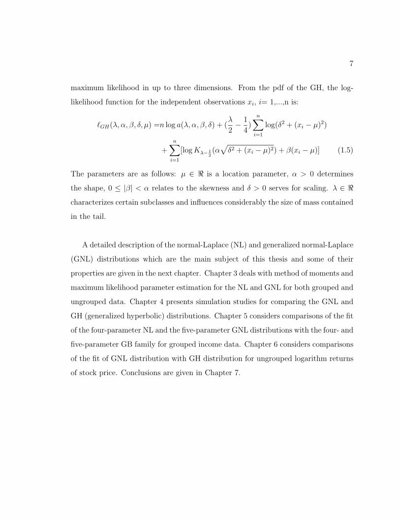
maximum likelihood in up to three dimensions. From the pdf of the GH, the log-

likelihood function for the independent observations xi, i= 1,...,n is:

`GH(λ, α, β, δ, µ) =n log a(λ, α, β, δ) + (λ

2− 1

4)

n∑i=1

log(δ2 + (xi − µ)2)

+n∑i=1

[logKλ− 12(α√δ2 + (xi − µ)2) + β(xi − µ)] (1.5)

The parameters are as follows: µ ∈ < is a location parameter, α > 0 determines

the shape, 0 ≤ |β| < α relates to the skewness and δ > 0 serves for scaling. λ ∈ <

characterizes certain subclasses and influences considerably the size of mass contained

in the tail.

A detailed description of the normal-Laplace (NL) and generalized normal-Laplace

(GNL) distributions which are the main subject of this thesis and some of their

properties are given in the next chapter. Chapter 3 deals with method of moments and

maximum likelihood parameter estimation for the NL and GNL for both grouped and

ungrouped data. Chapter 4 presents simulation studies for comparing the GNL and

GH (generalized hyperbolic) distributions. Chapter 5 considers comparisons of the fit

of the four-parameter NL and the five-parameter GNL distributions with the four- and

five-parameter GB family for grouped income data. Chapter 6 considers comparisons

of the fit of GNL distribution with GH distribution for ungrouped logarithm returns

of stock price. Conclusions are given in Chapter 7.

Chapter 2

The Normal-Laplace and Generalized Normal

Laplace Distributions

2.1 The Laplace Distribution

The classical Laplace distribution with mean zero and variance σ2 was introduced

by Laplace in 1774 (see e.g. Kotz et al., 2001). The distribution is symmetrical and

leptokurtic, which means its shape is more peaked (has higher kurtosis) than that of

the normal distribution. It has a characteristic function (ch.f)

φ(t) =1

1 + σ2t2

2

(2.1)

and pdf

f(x) =

√2

2σe−√

2|x|/σ, x ∈ <, σ > 0. (2.2)

This distribution has been used for modelling data that have heavier tails than those

of the normal distribution.

The skew-Laplace distribution (or asymmetric Laplace) is an asymmetric version

of the Laplace distribution (Kotz et al., 2001). Its pdf can be written

f(x) =

αβα+β

exp−α(x−µ) x ≥ µ

αβα+β

expβ(x−µ) x < µ(2.3)

where µ is a location parameter and the parameters α and β influence right and left-

tails, respectively. A value of α greater than β results in less probability to the right

side of µ than to the left side; the opposite is of course true if β is greater than α. If

α = β, the distribution is symmetrical.

9

2.2 Normal Laplace Distribution

The normal Laplace (NL) distribution (Reed and Jorgensen, 2004) is a relatively

new distribution that belongs to the generalized normal Laplace (GNL) distribution

family (Reed, 2000). It has been used to describe the distribution of incomes, particle

sizes, oil-field sizes, city sizes, and other phenomenons. It results from the convolution

of independent normal and asymmetric Laplace components.

Xd= Z +W (2.4)

where Z is a normally distributed random variable with mean µ and variance σ2, and

W has the asymmetric Laplace distribution (2.3) with parameters µ = 0, α and β.

The cumulative distribution function (cdf) of the NL distribution can be showed to

be (Reed and Jorgensen, 2004)

F (x) = Φ(x− µσ

)− φ(x− µσ

)βR(ασ − (x− µ)/σ)− αR(βσ + (x− µ)/σ)

α + β(2.5)

where Φ and φ are the cdf and pdf of a standard normal random variable and R is

Mills′ ratio:

R(z) =Φc(z)

φ(z)=

1− Φ(z)

φ(z)(2.6)

The cdf above depends on four parameters: µ ∈ < is a location parameter; σ > 0

is the scale parameter for the normal component; α > 0 and β > 0 are parameters

controlling tail behaviour. Since the likelihood function for grouped data is expressed

in terms of cdf, equation (2.4) above is very useful when fitting to data.

10

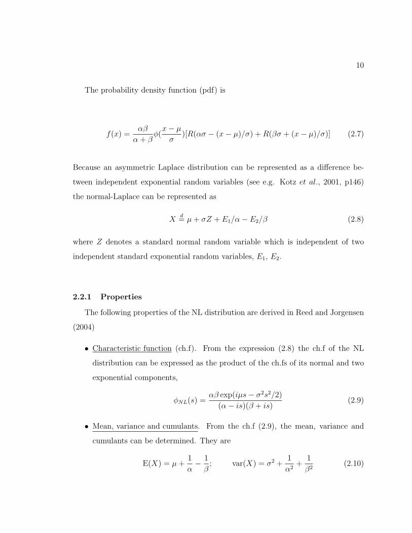
The probability density function (pdf) is

f(x) =αβ

α + βφ(x− µσ

)[R(ασ − (x− µ)/σ) +R(βσ + (x− µ)/σ)] (2.7)

Because an asymmetric Laplace distribution can be represented as a difference be-

tween independent exponential random variables (see e.g. Kotz et al., 2001, p146)

the normal-Laplace can be represented as

Xd= µ+ σZ + E1/α− E2/β (2.8)

where Z denotes a standard normal random variable which is independent of two

independent standard exponential random variables, E1, E2.

2.2.1 Properties

The following properties of the NL distribution are derived in Reed and Jorgensen

(2004)

• Characteristic function (ch.f). From the expression (2.8) the ch.f of the NL

distribution can be expressed as the product of the ch.fs of its normal and two

exponential components,

φNL(s) =αβ exp(iµs− σ2s2/2)

(α− is)(β + is)(2.9)

• Mean, variance and cumulants. From the ch.f (2.9), the mean, variance and

cumulants can be determined. They are

E(X) = µ+1

α− 1

β; var(X) = σ2 +

1

α2+

1

β2(2.10)

11

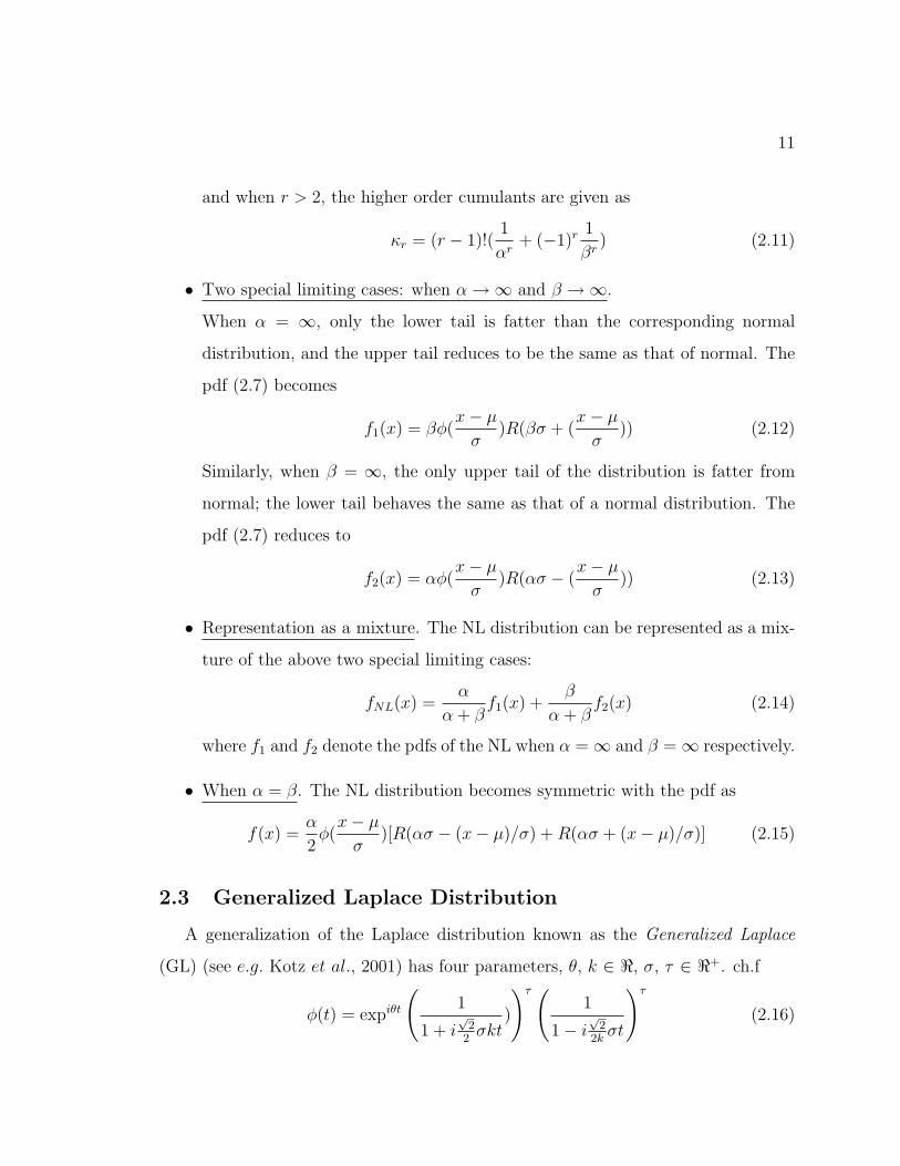
and when r > 2, the higher order cumulants are given as

κr = (r − 1)!(1

αr+ (−1)r

1

βr) (2.11)

• Two special limiting cases: when α→∞ and β →∞.

When α = ∞, only the lower tail is fatter than the corresponding normal

distribution, and the upper tail reduces to be the same as that of normal. The

pdf (2.7) becomes

f1(x) = βφ(x− µσ

)R(βσ + (x− µσ

)) (2.12)

Similarly, when β = ∞, the only upper tail of the distribution is fatter from

normal; the lower tail behaves the same as that of a normal distribution. The

pdf (2.7) reduces to

f2(x) = αφ(x− µσ

)R(ασ − (x− µσ

)) (2.13)

• Representation as a mixture. The NL distribution can be represented as a mix-

ture of the above two special limiting cases:

fNL(x) =α

α + βf1(x) +

β

α + βf2(x) (2.14)

where f1 and f2 denote the pdfs of the NL when α =∞ and β =∞ respectively.

• When α = β. The NL distribution becomes symmetric with the pdf as

f(x) =α

2φ(x− µσ

)[R(ασ − (x− µ)/σ) +R(ασ + (x− µ)/σ)] (2.15)

2.3 Generalized Laplace Distribution

A generalization of the Laplace distribution known as the Generalized Laplace

(GL) (see e.g. Kotz et al., 2001) has four parameters, θ, k ∈ <, σ, τ ∈ <+. ch.f

φ(t) = expiθt

(1

1 + i√

22σkt

)

)τ (1

1− i√

22kσt

)τ

(2.16)

12

Its probability density function (pdf) is:

f(x) =

√2e√

22σ

(1/k−k)(x−θ)√πστ+1/2Γ(τ)

(

√2|x− θ|k + 1/k

)τ−12Kτ− 1

2(

√2

2σ(1

k+ k)|x− θ|) (2.17)

where Kλ is the modified Bessel function of third kind with index λ. There are some

special cases associated with the distribution. For τ = 1, we have an asymmetric

Laplace, and for k = 1 and θ = 0, we obtain a symmetric Laplace distribution.

The pdf (2.17) can be written

f(x) = (αβ)τ exp

(β − α

2x

)(|x|

α + β

)τ−1/2

Kτ−1/2

(α + β

2|x|)

(2.18)

where α and β describe the left and right-tail shapes, and have the same role as α

and β in Laplace distribution; and τ is a parameter relating to the peakedness of the

pdf. We shall denote such a distribution by GL(α, β, τ)

Figure 2.1 (a) and (b) illustrate the effect of the parameters, α, β and τ . Using

the parameterization (2.18), Figure 2.1 (a) shows the effect of τ on the shape of the

distribution. The three curves are for GL(1, 1, τ) with τ = 0.8 (red), 1 (blue), and

2 (yellow). Figure 2.1 (b) shows the effect of α and β with GL(α, β, 0.8) where α=

3 and β =1 (green), and α= 1 and β =5 (light blue). Figure 2.1 (c) shows the pdf

curves for the GL(1, 1, 0.8) (Green), GL(1, 1, 1) and Normal (0, 1) (black dotted)

distributions.

13

−4 −2 0 2 4

0.0

0.2

0.4

0.6

The Effect of Tau

ax

f(x)

tau=0.8tau=1tau=2

−4 −2 0 2 4

0.0

0.5

1.0

1.5

The Effect of alpha and beta

bx

f(x)

alpha=3, beta=1alpha=1, beta=5

−4 −2 0 2 4

0.0

0.2

0.4

0.6

Comparison of GL and Normal distribution

cx

f(x)

GL (tau=0.8)GL (tau=1)Normal

Figure 2.1: The effect of the parameters of GL and the comparison of GL and normal

distributions.

2.4 Generalized Normal Laplace (GNL) Distribution

The generalized normal Laplace (GNL) distribution was introduced by Reed (2004)

and has been used for modelling financial logarithmic price returns. A closed-form

of the pdf of the GNL has not been found; however, it can be obtained from the

convolution of independent normal and generalized Laplace distributions. The GNL

14

distribution is defined as a random variable X with ch.f

φGNL(s) =

[αβ exp(iµs− σ2s2/2)

(α− is)(β + is)

]ρ(2.19)

where µ ∈ < a location parameter, σ ∈ <+ is the scale parameter for the normal

component, α, β ∈ <+are parameters influencing tail behavior and ρ ∈ <+ is a shape

parameter (ρ corresponds to the parameter τ in GL component, (2.18)).

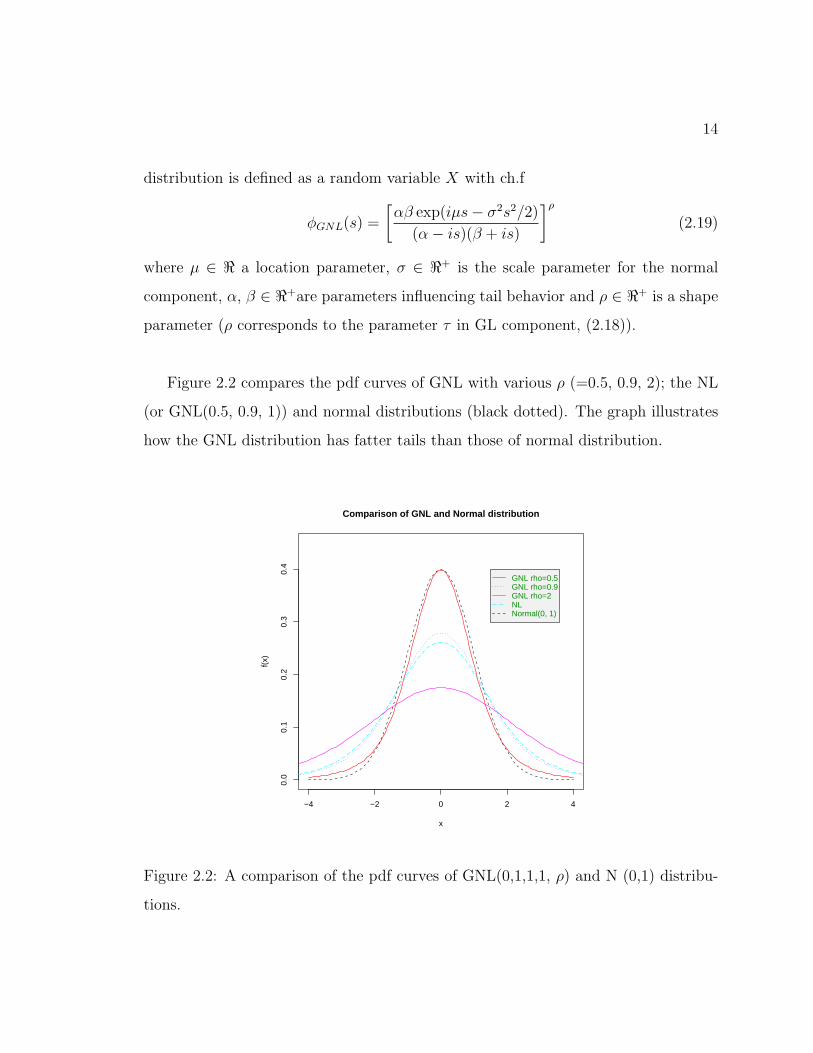
Figure 2.2 compares the pdf curves of GNL with various ρ (=0.5, 0.9, 2); the NL

(or GNL(0.5, 0.9, 1)) and normal distributions (black dotted). The graph illustrates

how the GNL distribution has fatter tails than those of normal distribution.

−4 −2 0 2 4

0.0

0.1

0.2

0.3

0.4

Comparison of GNL and Normal distribution

x

f(x)

GNL rho=0.5GNL rho=0.9GNL rho=2NLNormal(0, 1)

Figure 2.2: A comparison of the pdf curves of GNL(0,1,1,1, ρ) and N (0,1) distribu-

tions.

15

−5 0 5 10

0.00

0.05

0.10

0.15

0.20

0.25

0.30

The Effect of mu

x

f(x)

mu=0mu=1mu=2

Figure 2.3: The pdf curves of three GNL distributions with σ2=1, α=1, β=2 and

ρ=1.2, when µ=0 (red), µ=1 (blue dotted) and µ=2 (black)

The role played by location parameter µ is clearly shown in Figure 2.3: an increase

in µ moves the pdf curve of GNL distribution rightward horizontally.

16

−5 0 5

0.00

0.05

0.10

0.15

0.20

0.25

0.30

0.35

The Effect of Sigma

x

f(x)

sigma=1sigma=2sigma=3

Figure 2.4: The pdf curves of three GNL distributions with µ=0, α=1, β=2, and

ρ=1.2, when σ=1 (red), σ=2 (blue dotted) and σ=3 (black)

Figure 2.4 shows the effect of the parameter σ; with an increase in σ, the pdf

curve becomes wider and flatter the same time.

The parameter, α, affects the upper tail behavior of the GNL distribution: Figure

2.5 shows the change in the upper tail as α increases. Small values of α correspond

to a fat upper tail. When α =∞, the upper tail of the distribution reduces to that of

a normal distribution. Figure 2.6 shows similar behavior to the parameter β having

effects on the lower tail.

17

−5 0 5

0.00

0.05

0.10

0.15

0.20

0.25

0.30

0.35

The Effect of alpha

x

f(x)

alpha=0.5alpha=1alpha=2

Figure 2.5: The pdf curves of three GNL distributions with µ=0, σ=1, β=2, and

ρ=1.2, when α=1 (red), α=2 (blue dotted) and α=0.5 (black)

−5 0 5

0.00

0.05

0.10

0.15

0.20

0.25

0.30

The Effect of beta

x

f(x)

beta=0.6beta=2beta=10

Figure 2.6: The pdf curves of three GNL distributions with µ=0, σ=1, α=1, and

ρ=1.2, when β=2 (red), β=10 (blue dotted) and β=0.6 (black)

18

−10 −5 0 5 10

0.00

0.05

0.10

0.15

0.20

0.25

0.30

0.35

The Effect of rho

x

f(x)

rho=0.75rho=1rho=2rho=3.2

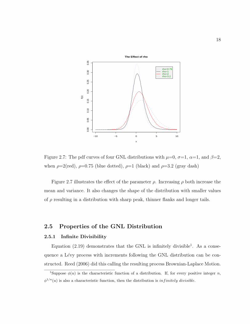
Figure 2.7: The pdf curves of four GNL distributions with µ=0, σ=1, α=1, and β=2,

when ρ=2(red), ρ=0.75 (blue dotted), ρ=1 (black) and ρ=3.2 (gray dash)

Figure 2.7 illustrates the effect of the parameter ρ. Increasing ρ both increase the

mean and variance. It also changes the shape of the distribution with smaller values

of ρ resulting in a distribution with sharp peak, thinner flanks and longer tails.

2.5 Properties of the GNL Distribution

2.5.1 Infinite Divisibility

Equation (2.19) demonstrates that the GNL is infinitely divisible1. As a conse-

quence a Levy process with increments following the GNL distribution can be con-

structed. Reed (2006) did this calling the resulting process Brownian-Laplace Motion.

1Suppose φ(u) is the characteristic function of a distribution. If, for every positive integer n,

φ1/n(u) is also a characteristic function, then the distribution is infinitely divisible.

19

For such a process St the increments Sw+t − Sw have a characteristic function:[αβ exp(iµs− σ2s2/2)

(α− is)(β + is)

]ρt= [φ0(s)]t (2.20)

where φ0(s) is the characteristic function of a GNL variate of the form (2.19). It ca

be seen that the length t of the time increment affects only the exponent parameter

ρ of the GNL distribution.

2.5.2 Mean, Variance and Cumulants

The cumulants κn of a distribution are defined as (Abramowitz and Stegun, 1972,

p. 928)

log(φ(s)) =∞∑n=1

κn(is)n

n!(2.21)

In particular, the first and second cumulants are the mean and variance of the

distribution. For a GNL distribution

log(φGNL(s)) = ρµis+ ρσ2 (is)2

2!+ log(

α

α− is)ρ + log(

β

β + is)ρ

= ρµis+ ρσ2 (is)2

2!+ ρ log

α

α− is+ ρ log

β

β + is

= isρ(µ+1

α− 1

β) +

1

2!(is)2ρ(σ2 +

1

α2+

1

β2) +

1

3!(is)3ρ(

2

α3− 2

β3) + ...

(2.22)

using the Maclaurin series expansions of log αα−is and log β

β+is. We thus obtain the

mean and variance

E(X) = ρ(µ+1

α− 1

β); var(X) = ρ(σ2 +

1

α2+

1

β2) (2.23)

and the higher order cumulant functions ( r > 2)

κr = ρ(r − 1)!(1

αr+ (−1)r

1

βr) (2.24)

20

−5 0 5

0.00

0.05

0.10

0.15

0.20

0.25

0.30

0.35

The Effect of alpha

x

f(x)

alpha=0.5alpha=1alpha=2

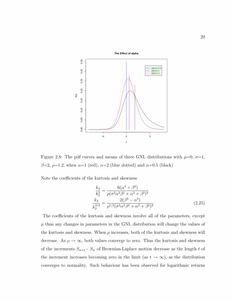
Figure 2.8: The pdf curves and means of three GNL distributions with µ=0, σ=1,

β=2, ρ=1.2, when α=1 (red), α=2 (blue dotted) and α=0.5 (black)

Note the coefficients of the kurtosis and skewness

k4

k22

=6(α4 + β4)

ρ(σ2α2β2 + α2 + β2)2

k3

k3/22

=2(β3 − α3)

ρ1/2(σ2α2β2 + α2 + β2)2(2.25)

The coefficients of the kurtosis and skewness involve all of the parameters, except

µ thus any changes in parameters in the GNL distribution will change the values of

the kurtosis and skewness. When ρ increases, both of the kurtosis and skewness will

decrease. As ρ → ∞, both values converge to zero. Thus the kurtosis and skewness

of the increments Sw+t - Sw of Brownian-Laplace motion decrease as the length t of

the increment increases becoming zero in the limit (as t → ∞), as the distribution

converges to normality. Such behaviour has been observed for logarithmic returns

21

on financial assets. From the expression for the skewness, it can be seen that α and

β determine in which direction the pdf will skew. If α > β, the GNL distribution

is skewed to the left, and vice versa. If α = β, then the GNL distribution is symmetric.

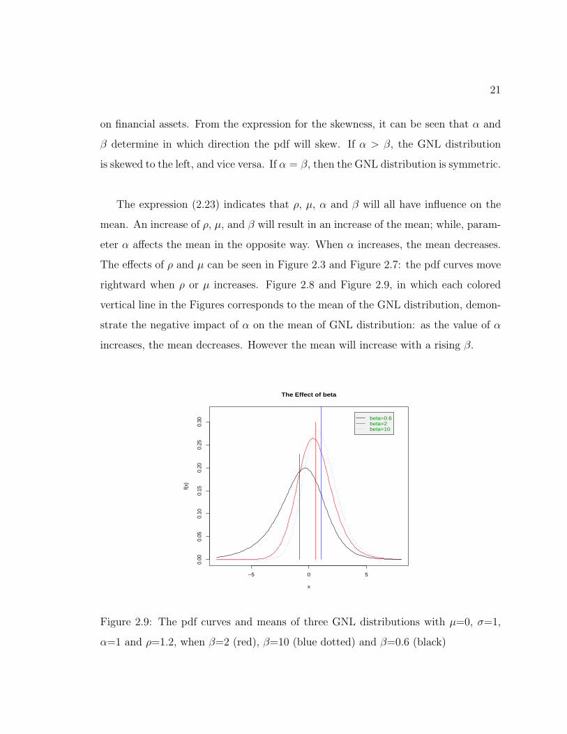
The expression (2.23) indicates that ρ, µ, α and β will all have influence on the

mean. An increase of ρ, µ, and β will result in an increase of the mean; while, param-

eter α affects the mean in the opposite way. When α increases, the mean decreases.

The effects of ρ and µ can be seen in Figure 2.3 and Figure 2.7: the pdf curves move

rightward when ρ or µ increases. Figure 2.8 and Figure 2.9, in which each colored

vertical line in the Figures corresponds to the mean of the GNL distribution, demon-

strate the negative impact of α on the mean of GNL distribution: as the value of α

increases, the mean decreases. However the mean will increase with a rising β.

−5 0 5

0.00

0.05

0.10

0.15

0.20

0.25

0.30

The Effect of beta

x

f(x)

beta=0.6beta=2beta=10

Figure 2.9: The pdf curves and means of three GNL distributions with µ=0, σ=1,

α=1 and ρ=1.2, when β=2 (red), β=10 (blue dotted) and β=0.6 (black)

22

The nature of the tails can be determined by the order of the poles of its char-

acteristic (or moment generating) function (Reed, 2004), which are given in table

2.5.1

Table 2.5.1 Description for the tails of the GNL distribution

Limit pdf

x→∞ f(x) ∼ c1xρ−1e−αx

x→ −∞ f(x) ∼ c2(−x)ρ−1eβx

where c1 and c2 are constants. The parameter ρ controls the thickness of the tails.

For ρ < 1, both tails are fatter than the corresponding exponential distribution; for

ρ= 1, they are like exponential tails; and for ρ > 1, they are thinner than those of

exponential.

The GNL distributions are closed under linear transformation: i.e. if X ∼GNL(µ,

σ2, α, β, ρ), then a + bX ∼ GNL(bµ + a/ρ, b2σ2, α/b, β/b, ρ), where a and b are

constants.

When µ = σ2 = 0, the GNL distribution has ch.f[αβ

(α− is)(β + is)

]ρ(2.26)

which is that of the generalized Laplace distribution (2.18)

If ρ = 1, the GNL distribution reduces to the normal Laplace (NL) distribution with

four parameters.

2.6 Numerical determination of the pdf and cdf of the GNL

In this section, we present three methods of numerically determining the pdf and

cdf of the GNL distributions.

23

2.6.1 Using the Representation as a Convolution

The characteristic function (2.19) can be written

φGNL(s) = exp(ρµis− ρσ2s2/2)

[α

α− is

]ρ [β

β + is

]ρ(2.27)

This is the product of the characteristic function of the normal distribution with

parameters µ and σ2 and that of generalized Laplace distribution (2.16). It follows

that the GNL distribution is that of the convolution of normal N(ρµ, ρσ2) and

GL(α , β, ρ) distributions

Xd= W + U, W ∼ N(ρµ, ρσ2), U ∼ GL(α, β, ρ) (2.28)

Furthermore ( θθ−is)

ρ is the ch.f of a gamma random variable with shape parameter

ρ and scale parameter 1θ. Thus the last two terms of (2.27) are the ch.fs of (i) a

gamma random variable with shape parameter ρ and scale parameter 1α

and (ii) the

negative of a gamma random variable with shape parameter ρ and scale parameter

1β. It follows from (2.27) that a GNL random variable, X ∼GNL(µ, σ2, α, β, ρ) can

be represented as a convolution

Xd= ρµ+ σ

√ρZ +

1

αG1 −

1

βG2 (2.29)

where Z, G1 and G2 are independent with Z∼N(0,1) and G1, G2 are gamma random

variables with scale parameter θ = 1 and shape parameter ρ. i.e with pdf given by

γ(u)= 1Γ(ρ)

uρ−1e−u

Closed-form expressions for the pdf and cdf of the family of GNL distributions have

not been found except when ρ = 1. However, the pdf (and cdf) can be obtained a

numerically using the convolution (2.28) as (2.29) to represent the pdf of the GNL

f(x) =

∫ ∞−∞

fW (x− u)fU(u)du (2.30)

24

and the cdf of GNL is

F (x) =

∫ ∞−∞

FW (x− u)fU(u)du (2.31)

where fU(u) is the pdf of generalized Laplace distribution (2.18), and fW (w) and

FW (w) are the pdf and cdf of a normal distribution with mean ρµ and variance ρσ2.

The integrals (2.30) and (2.31) can be evaluated numerically to obtain the pdf and

cdf of the GNL distribution.

2.6.2 Numerical Inversion of Characteristic Function

The ch.f of GNL (2.27) can be expressed

φGNL(s) = r(s) exp(iθ(s))

(2.32)

where r(s) and θ(s) are the modulus and argument of the ch.f of the random variables

of (2.27).

The ch.f can be inverted to obtain the pdf of GNL (see e.g. Knight and Satchell,

2001, p.285)

fGNL(x) =1

2π

∫ ∞−∞

e−isxφ(s)ds

=1

2π

∫ ∞−∞

r(s)ei(θ(s)−sx)ds

=1

π

∫ ∞0

r(s)(cos(θ(s)− sx) + i sin(θ(s)− sx))ds

=1

π

∫ ∞0

r(s)(cos(θ(s)− sx)ds (2.33)

using the fact that f(x) is a real, so that the imaginary part of the integral will be zero.

25

The cdf of GNL can be obtained by inversion of the ch.f as (Shephard, 1991)

FGNL(x) =1

2+

1

2π

∫ ∞0

eisxφ(−s)− e−isxφ(s)

isds

(2.34)

Since φ(s) = r(s)eiθ(s) and eisxφ(−s) − e−isxφ(s) = i2r(s) sin(sx − θ(s)), the cdf of

GNL is

FGNL(x) =1

2+

1

π

∫ ∞0

r(s)

ssin(sx− θ(s))ds (2.35)

The integrals (2.33) and (2.35) can be evaluated numerically to obtain the pdf and

cdf of GNL.

2.6.3 Using the representation as a Normal mean-variance mixture

The Normal variance-mean mixture representation of the GNL derives from it

being the distribution at the state of the Brownian motion dx = νdt + τdw with

initial state x0∼ N(µ0, σ20) observed at a random time T independent of the Brownian

motion with T ∼ Gamma(λ, ρ). By re-scaling time it is also the state of the Brownian

motion dx = νλdt + τ√

λdw at time T ′=λT ∼ Gamma(1, ρ). For a fixed time t the

state of this latter Brownian motion is

X(t) ∼ N (µ+ νλt, σ2+ τ2

λt)

so that the state after gamma-distributed time is a “mean-variance” mixture of normal

distributions with mixing parameter t.

Re-parameterizing, letting 1α

- 1β

= νλ

and 2αβ

= τ2

λone gets

X(t) ∼ N (µ + ( 1α

- 1β)t, σ2 + 2

αβt)

so that, the pdf of GNL is

fGNL(x) =

∫ ∞0

1√2π(σ2 + 2

αβt)

2 exp

(−(x− (µ+ (

1

α− 1

β)t))2/2(σ2 +

2

αβt)2

)g(t)dt

(2.36)

26

where g(t) = 1Γ(ρ)

tρ−1et is the pdf of a gamma distribution with scale-parameter 1 and

shape parameter ρ. This integral can be evaluated numerically.

Chapter 3

Methods of Estimation

We consider estimation for both grouped and ungrouped data. In the applications the

ungrouped data come from the logarithmic returns of stock prices, and the grouped

data from household incomes data.

Ungrouped Data

To fit the GNL model to ungrouped data (e.g. logarithmic returns), one can estimate

model parameters using Maximum Likelihood Estimation (MLE), or the Method of

Moments Estimation (MME). One could also consider Bayesian methods, but these

will not be discussed in this thesis.

3.1 Method of Moments

Although the Method of Moments Estimation (MME) is less efficient than MLE, it

is usually computationally simpler. MME is performed by solving a set of equations

obtained by equating population moments to sample moments. The kth-moment

of a random variable is E(Xk), and this must be expressed as a function of model

parameters. The kth sample moment is mk=1n

∑ni=1 X

ki . The MME estimates for i.i.d

observation x1,...,xn are obtained by solving (for the parameters θ˜) following system

of equations

Eθ˜(Xk) =

1

n

n∑i=1

Xki k = 1, ..., p. (3.1)

where θ˜ is a p-vector of parameters.

The cumulants of a distribution are defined in terms of the cumulant generating

28

function (cgf)

KX(t) = logMX(t) (3.2)

where MX(t) is the moment generating function

MX(t) = E(etx) (3.3)

The jth cumulant κj is the coefficient of tj/j! in the Taylor series expansion of Kx(t)

i.e

κj =djKx(t)

dtj|t=0 (3.4)

Since there is a one-to-one relationship between cumulants and moments one can find

method of moments estimates of parameters by solving simultaneously the p equations

resulting from setting the first p cumulants of the distribution equal to their sample

equivalents. i.e

κj(θ˜) = kj j = 1, ..., p (3.5)

where kj is the coefficient of tj/j! the Taylor series expansion of the sample cgf i.e of

kx(t) = log

[1

n

n∑i=1

etxi

](3.6)

i.e

kj =djkx(t)

dtj|t=0 (3.7)

Sample cumulants are related to sample moments in the same way as population

cumulants and moments are related. Precisely

k1 = m1

k2 = m2 −m21

k3 = 2m31 − 3m1m2 +m3

k4 = −6m41 + 12m2

1m2 − 3m22 − 4m1m3 +m4

k5 = 24m51 − 60m3

1m2 + 20m21m3 − 10m2m3 + 5m1(6m2

2 −m4) +m5 (3.8)

29

where mj is the jth sample moment. The first few sample cumulants can thus be

readily computed from the sample moments.

Reed (2004) determined the cumulants of the GNL as

κ1 = ρ(µ+1

α− 1

β)

κ2 = ρ(σ2 +1

α2+

1

β2)

κr = ρ(r − 1)!(1

αr+ (−1)r

1

βr) r = 3, 4... (3.9)

To find MMEs of the five parameters of the GNL thus involves solving for (µ, σ2, α,

β, ρ) simultaneously the five equations κ1=k1, κ2=k2,...,κ5=k5. With some simple

algebra (Reed, 2004) this can be reduced to solving (for α, β) the pair of equations

12k3(α−5 − β−5) = k5(α−3 − β−3), 4k4(α−5 − β−5) = k5(α−4 + β−4) (3.10)

from which the corresponding solution values of the other parameters can be obtained

as

ρ = k32!

1

α−3−β−3; σ2 = k2

ρ− α−2 − β−2 and µ = k1

ρ− α−1 + β−1

In the special case of a symmetric GNL distribution (α = β), the estimates of the

four parameters by method of moments, can be found analytically. The equation

(3.9) gives

κ1 = ρµ

κ2 = ρ(σ2 +2

α2)

κ3 = 0

κ4 = 3!ρ(2

α4)

κ6 = 5!ρ(2

α6) (3.11)

30

with higher odd-order cumulants all zero, i.e κ3=κ5=κ7= ... =0

From the above system, the estimates are (Reed, 2004)

α = β=√

20k4k6

; ρ = 1003

k34

k26

; σ2 = k2ρ− 2

α2 and µ = k1ρ

The parameter space for the GNL (µ, σ2, α, β, ρ) distribution is <⊗<4+. i.e the

four-parameters σ2, α, β, ρ are constrained to be positive, while µ can be any real

number. This can cause problems for the method of moments, because sometimes the

solution to the moment equations will fall outside of the parameter space. i.e result

in an estimate in which some of σ2, α, β and ρ are negative.

Method of moments estimation can also be applied to the ordinary NL distribution

(2.11) for which the third and fourth order cumulants are

κ3 = 2α−3 − 2β−3; κ4 = 6α−4 + 6β−4 (3.12)

MMEs for α and β can be found by solving numerically the pair of equations k3 =

κ3 and k4 = κ4 and the corresponding estimates of µ and σ can then be found as

µ = k1 - 1α

+ 1β

and σ2= k2 - ( 1α2 + 1

β2 )

3.2 Maximum Likelihood Estimation

Maximum likelihood estimation (MLE) is the “gold-standard” method for ob-

taining parameter estimates. The likelihood function is a mathematical expression

obtained as an arbitrary constant times the probability of observing the given data

regarded as a function of model parameters θ˜. Maximum likelihood (ML) estimates

are obtained by maximizing the function with respect to θ˜. It is usually more conve-

nient to maximize the log-likelihood function with respect to the model parameters.

For independent identically distributed observations, the likelihood is the product of

31

the probability density (or mass) function f(x; θ˜) evaluated at each of the observed

data value. i.e

L(θ˜) =∏i

f(xi; θ˜) (3.13)

and the log-likelihood is

`(θ˜) =∑i

log f(xi; θ˜) (3.14)

There is no closed-form expression for the probability density function (pdf) of the

GNL distribution so one cannot obtain a closed-form for the likelihood or log-likelihood.

One can however evaluate it numerically for given values of θ˜ (and given data). In

this thesis we consider three methods of performing this numerical calculation. They

are (see section 2.6)

• (a) Convolution of normal and generalized Laplace pdfs

• (b) Inversion of the characteristic function

• (c) Using the representation of the GNL distribution as a normal mean-variance

mixture.

To evaluate the log-likelihood for a single value of the parameters θ˜, n numerical

integrations (using method (a), (b) or (c)) must be conducted (where n is number of

observations in the sample).

To find MLEs involves numerically maximizing the log-likelihood function. This has

been performed using the R function optim in the stats package.

For the ordinary NL distribution a closed form of the pdf and hence of the log-

likelihood exist. Precisely for independent observations y1, y2, ..., yn from NL(µ, σ2,

32

α, β) the log likelihood function is

` = n logα + n log β − n log(α + β) +n∑i=1

log[R(pi) +R(qi)] (3.15)

where pi = ασ− (yi− µ)/σ and qi = βσ+ (yi− µ)/σ, and R is the Mills′ ratio (2.6)

of the complementary cumulative distribution function (cdf) to the pdf of a standard

normal distribution.

This can be maximized analytically over µ to obtain

µ = y − 1

α+

1

β(3.16)

and a profile likelihood

ˆ(α, β, σ2) =n logα + n log β − n log(α + β) +n∑i=1

φ(yi − y + 1/α− 1/β

σ2)+

n∑i=1

log[R(ασ2 − yi − y + 1/α− 1/β

σ2) +R(βσ2 +

yi − y + 1/α− 1/β

σ2)]

(3.17)

This must be maximized numerically (e.g using the function optim in R) to obtain

maximum likelihood estimates of parameters. Another approach is to use the EM-

algorithm (Reed and Jorgensen 2004), although there seems to be little to be gained

in terms of computation time.

Measurement of the performance

Quantile-quantile (Q-Q) plots provide a way of visually assessing the fit a distri-

bution to ungrouped data. In a Q-Q plot, if the resulting points lie roughly on the

line of slope 1, then the compared distribution fits the data well. Q-Q plots are ob-

tained by plotting the quantiles of the data of the empirical distribution against the

theoretical quantiles using MLEs of the parameters. The empirical quantiles are just

the sorted observations. The theoretical quantile Qi corresponding to the ith ordered

observation is obtained by solving

33

FGNL(Qi) = pi

where pi = (i− 0.5)/n, therefore

Qi = F−1GNL(pi) (3.18)

Unfortunately no closed-form exists for the inverse of the c.d.f of the GNL distribution,

so equation (3.18) has to be solved numerically.

Grouped data

We now consider the grouped data with boundaries 0 < x1 < x2.... Since grouped in-

come data available from the Luxembourg Income Study (http : //www.lisproject.org)

are in the form of percentiles of the distribution, we consider the likelihood for such

data is proportional to the joint distribution of the order statistics corresponding

to the empirical percentiles. For example, if x(1), x(2), ..., x(19) correspond to 5th,

10th,..., 95th percentiles of a sample of size N, then the log-likelihood is of the form

`(θ˜) =19∑i=1

log f(log x(i)) +N

20

20∑i=1

log(Pi(θ˜)) + C (3.19)

where Pi(θ˜) = F (log(x(i)); θ˜)−F (log(x(i−1)); θ˜); F () denotes the cumulative distribu-

tion function; θ˜ is the parameter vector; x(i) and x(i−1) are the upper and lower bounds

of the ith of 20 data groups, and N is the total number of observations. Typically N

will be a very large number, and the first part of the summation is relatively much

smaller than that of second part. In previous studies of fitting income distribution it

has been ignored, with simply the multinomial log likelihood (where all frequencies

= N/20)

(N/20)20∑i=1

log(Pi(θ˜)) (3.20)

34

being maximized.

Goodness-of-Fit for grouped data

The sum of squared errors (SSE), sum of absolute errors (SAE), and chi-square (χ2)

goodness-of-fit statistic and the maximized log-likelihood are four measures used in

previous studies to compare the fit of parametric income distribution models. The

SSE, SAE and χ2 are defined as

SSE =N∑i=1

{niN− Pi(θ˜)

}2

(3.21)

SAE =N∑i=1

∣∣∣niN− Pi(θ˜)

∣∣∣ (3.22)

χ2 = NN∑i=1

[{niN− Pi(θ˜)

}2

/Pi(θ˜)]

(3.23)

where θ˜ denotes the estimated parameters. Note that one would not use the χ2 statis-

tic based on proportions to test for goodness of fit. We use this form of it simply to

make comparisons with results of Bandourian et al. (2002), who used the χ2 statistic

in this form. In this thesis we compare the fit of the four-parameter NL with the best

four-parameter fit obtained to date, that of the generalized beta (GB2) distribution

(McDonald, 1984); and compare the five-parameter GNL with best five-parameter

model obtained to date, that of the GB (McDonald and Xu, 1995).

3.3 Nelder-Mead Method: Multi-dimensional Maximization

Method

The R function optim includes several methods of optimization. The Nelder-Mead

method, which does not require derivatives, has been used in this thesis. The method

35

is simple, intuitive and relatively stable in approaching the optimum and can be

applied to discontinuous problems. It is based on evaluating a function at the vertices

of a simplex, then iteratively shrinking the simplex as better points are found and

repeat the process until some desired bounds are obtained (Nelder and Mead, 1965).

Ideally the optimum will not depend on the starting values. However if the likelihood

possesses more than one local maximum the point to which the algorithm converges

may depend on the starting value. To check whether this is the case optimization

was run several times using different starting values.

Chapter 4

Simulation Studies for The GNL distribution

One way to examine the performance of an estimation procedure is to apply it to

simulated data with a known distribution. In this chapter, we utilize GNL simulation

to assess the results of estimation. In addition, we fit a generalized hyperbolic (GH)

distribution to GNL simulated data and fit the GNL distribution to simulated GH

data.

4.1 Simulating GNL Data

Pseudo random variables from a GNL distribution can be simulated from (2.29)

directly. This involves simulating random variables from the three independent dis-

tributions, namely the standard normal Z and two gamma distributions G1, G2 with

scale parameter θ = 1 and shape parameter ρ. A GNL random variable X ∼GNL(µ,

σ2, α, β, ρ) is then obtained as

X = ρµ+ σ√ρZ + 1

αG1 − 1

βG2

Fitting to ungrouped data sometimes resulted in difficulties with multiple local max-

ima, with very similar values. As an alternative the data were grouped and the model

fitted to grouped data. This seemed to eliminate difficulties with multiple maxima.

Further research is needed to investigate the problem with multiple maxima. The

process of the simulation was as follows:

• Generate 1,000 artificial GNL distributed observations, for given parameter val-

ues e.g generate 1000 (i.d) GNL (0.1, 0.4, 0.2, 0.3, 0.2) deviates.

37

• Group the observations into 20 equal-frequency intervals.

• Estimate the parameters using the MLE estimation method for grouped data.

• Compare results from the Q-Q plots.

The following table shows estimates obtained via numerical maximization for differ-

ent starting values of the optimization routine. In addition,Q-Q plots of sample and

fitted theoretical quantiles are given. In all cases shown the parameter values used in

the simulation were µ=0.1, σ2=0.42, α=0.2, β=0.3 and ρ=0.2.

Table 4.1 GNL (using MLE) fitted to the simulated GNL data

GNL(starting values) Max ` µ σ2 α β ρ

(0.1,0.4,0.9,1,0.2) 3021.452 0.0266 0.0379 0.2344 0.3441 0.2122

(-0.3,0.4,1,0.5,0.6) 3021.452 0.0266 0.0379 0.2344 0.3441 0.2122

(0.1,0.6,0.1,0.1,0.7) 3021.452 0.0266 0.0379 0.2344 0.3441 0.2122

(-1,0.9,0.3,0.4,0.5) 3021.452 0.0266 0.0379 0.2344 0.3441 0.2122

Table 4.1 indicates that the routine converges to the same maximum for differ-

ent starting values. In addition, the MLEs are fairly close to the true values. The

standard errors of the estimators are: µ (0.0423), σ2 (0.0255), α (0.0248), β (0.0275),

ρ (0.0161). Furthermore, the Q-Q plot in the Figure 4.1 shows a satisfactory fit.

This and other similar Q-Q plots using simulated data were used as a reference for

assessing the degree of deviation from a straight line that could be expected.

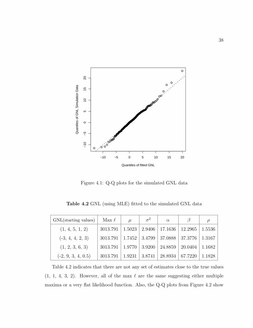
For some other choices of parameter values, e.g. GNL (1, 1, 4, 3, 2), multiple

maxima resulted

38

●● ●

●

●●●●●●

●●●●●●●

●●●●●●●●●●●●●●●

●●●●●●●●●●●●●●●●●●●●●●●●●●●●

●●●●●●●●●●●●●●●●●●●●●●●●●●●●●●●●●●●●●●●

●●●●●●●●●●●●●●●●●●●●●●●●●●●●●●●●●●●●●●●●●●●●●●●●●●●●●●●●●●●●●●●●●●●●●●●●●●●●●●●●●●●●●●●●●●●●●●●●●●●●●●●●●●●●●●●●●●●●●●●●●●●●●●●●●●●●●●●●●●●●●●●●●●●●●●●●●●●●●●●●●●●●●●●●●●●●●●●●●●●●●●●●●●●●●●●●●●●●●●●●●●●●●●●●●●●●●●●●●●●●●●●●●●●●●●●●●●●●●●●●●●●●●●●●●●●●●●●●●●●●●●●●●●●●●●●●●●●●●●●●●●●●●●●●●●●●●●●●●●●●●●●●●●●●●●●●●●●●●●●●●●●●●●●●●●●●●●●●●●●●●●●●●●●●●●●●●●●●●●●●●●●●●●●●●●●●●●●●●●●●●●●●●●●●●●●●●●●●●●●●●●●●●●●●●●●●●●●●●●●●●●●●●●●●●●●●●●●●●●●●●●●●●●●●●●●●●●●●●●●●●●●●●●●●●●●●●●●●●●●●●●●●●●●●●●●●●●●●●●●●●●●●●●●●●●●●●●●●●●●●●●●●●●●●●●●●●●●●●

●●●●●●●●●●●●●●●●●●●●●●●●●●●●●●●●●●●●●●●●●●●●●●●●●●●●●●●●●●●●●●●●●●●●●●●●●●●●●●●●●●●●●●●●●●●●●●●●●●●●●●●●●●●●●●●●●●●●●●●●●●●●●●●●●●●●●●●●●●●●●●●●●●●●●●●●●●●●●●●●●●●●●●●●●●●●●●●●●●●●●●●●●

●●●●●●●●●●●●●●●●●●●●●●●●●●●●●●●●●●●●●●●●●●●●●●●●●●●●●●●●●●●●●●●●●●●●●●●●●●●●●●●●●●●●●●●●●●●●●●●●●●●●●●●●●●●●●●●●●●●●●

●●●●●●●●●●●●●●●●●●●●●●●●●●

●●●●●●●●●●●●●●●●●

●●●●●●●

●●●●●●

●●

●

●●

●

−10 −5 0 5 10 15 20

−10

−5

05

1015

20

Quantiles of fitted GNL

Qua

ntile

s of

GN

L S

imul

atio

n D

ata

Figure 4.1: Q-Q plots for the simulated GNL data

Table 4.2 GNL (using MLE) fitted to the simulated GNL data

GNL(starting values) Max ` µ σ2 α β ρ

(1, 4, 5, 1, 2) 3013.791 1.5023 2.9406 17.1636 12.2965 1.5536

(-3, 4, 4, 2, 3) 3013.791 1.7452 3.4799 37.0888 37.3776 1.3167

(1, 2, 3, 6, 3) 3013.791 1.9770 3.9200 24.8859 20.0404 1.1682

(-2, 9, 3, 4, 0.5) 3013.791 1.9231 3.8741 28.8934 67.7220 1.1828

Table 4.2 indicates that there are not any set of estimates close to the true values

(1, 1, 4, 3, 2). However, all of the max ` are the same suggesting either multiple

maxima or a very flat likelihood function. Also, the Q-Q plots from Figure 4.2 show

39

●●●●●●●●●●●●●●●●●●

●●●●●●●●●●●●●●●●●●●●●●●●●●●●●●

●●●●●●●●●●●●●●●●●●●●●●●●●●●●●●●●●●●●●●●●●●●●●●●●●●

●●●●●●●●●●●●●●●●●●●●●●●●●●●●●●●●●●●●●●●●●●●●●●●●●●●●●●●●●●●●●●●●●●●●●●●●●●●●●●●●●●●●●●●●●●●●●

●●●●●●●●●●●●●●●●●●●●●●●●●●●●●●●●●●●●●●●●●●●●●●●●●●●●●●●●●●●●●●●●●●●●●●●●●●●●●●●●●●●●●●●●●●●●●●●●●●●●●●●●●●●

●●●●●●●●●●●●●●●●●●●●●●●●●●●●●●●●●●●●●●●●●●●●●●●●●●●●●●●●●●●●●●●●●●●●●●●●●●●●●●●●●●●●●●●●●●●●●●●●●●●●●●●●●●●●●●●●●●●●●●●●●●●●●●●●●●●●●●●●

●●●●●●●●●●●●●●●●●●●●●●●●●●●●●●●●●●●●●●●●●●●●●●●●●●●●●●●●●●●●●●●●●●●●●●●●●●●●●●●●●●●●●●●●●●●●●●●●●●●●●●●●●●●●●●●●●●●●●●●●●●●●●●●●●●●●●●●●●●●●●●●●●●●●●●●●●●●●●●●●●●●●●●

●●●●●●●●●●●●●●●●●●●●●●●●●●●●●●●●●●●●●●●●●●●●●●●●●●●●●●●●●●●●●●●●●●●●●●●●●●●●●●●●●●●●●●●●●●●●●●●●●●●●●●●●●●●●●●●●●●●●●●●●●●●●●●●●●●●●●●●●●●●●●●●●●●●●●●●●●●●●●●●●●●●●●●●●●●●●●●●●●●●●●●●●●●

●●●●●●●●●●●●●●●●●●●●●●●●●●●●●●●●●●●●●●●●●●●●●●●●●●●●●●●●●●●●●●●●●●●●●●●●●●●●●●●●●●●●●●●●●●●●●

●●●●●●●●●●●●●●●●●●●●●●●●●●●●●●●●●●●●●●●●●●●●●●●●●●●●●●●●●

●●●●●●●●●●●●●●●●●●●●●●●●●●●●●●●●

●●●●●●●●●●●●●●●●●●●●●

●●●●●●●●●● ●

−4 −2 0 2 4 6 8

−6

−2

24

68

Quantiles of fitted GNL−−1

Qua

ntile

s of

GN

L S

imul

atio

n D

ata−

−1

●●●●●●●●●●●●●●●●●●

●●●●●●●●●●●●●●●●●●●●●●●●●●●●●●

●●●●●●●●●●●●●●●●●●●●●●●●●●●●●●●●●●●●●●●●●●●●●●●●●●

●●●●●●●●●●●●●●●●●●●●●●●●●●●●●●●●●●●●●●●●●●●●●●●●●●●●●●●●●●●●●●●●●●●●●●●●●●●●●●●●●●●●●●●●●●●●●

●●●●●●●●●●●●●●●●●●●●●●●●●●●●●●●●●●●●●●●●●●●●●●●●●●●●●●●●●●●●●●●●●●●●●●●●●●●●●●●●●●●●●●●●●●●●●●●●●●●●●●●●●●●

●●●●●●●●●●●●●●●●●●●●●●●●●●●●●●●●●●●●●●●●●●●●●●●●●●●●●●●●●●●●●●●●●●●●●●●●●●●●●●●●●●●●●●●●●●●●●●●●●●●●●●●●●●●●●●●●●●●●●●●●●●●●●●●●●●●●●●●●

●●●●●●●●●●●●●●●●●●●●●●●●●●●●●●●●●●●●●●●●●●●●●●●●●●●●●●●●●●●●●●●●●●●●●●●●●●●●●●●●●●●●●●●●●●●●●●●●●●●●●●●●●●●●●●●●●●●●●●●●●●●●●●●●●●●●●●●●●●●●●●●●●●●●●●●●●●●●●●●●●●●●●●

●●●●●●●●●●●●●●●●●●●●●●●●●●●●●●●●●●●●●●●●●●●●●●●●●●●●●●●●●●●●●●●●●●●●●●●●●●●●●●●●●●●●●●●●●●●●●●●●●●●●●●●●●●●●●●●●●●●●●●●●●●●●●●●●●●●●●●●●●●●●●●●●●●●●●●●●●●●●●●●●●●●●●●●●●●●●●●●●●●●●●●●●●●

●●●●●●●●●●●●●●●●●●●●●●●●●●●●●●●●●●●●●●●●●●●●●●●●●●●●●●●●●●●●●●●●●●●●●●●●●●●●●●●●●●●●●●●●●●●●●

●●●●●●●●●●●●●●●●●●●●●●●●●●●●●●●●●●●●●●●●●●●●●●●●●●●●●●●●●

●●●●●●●●●●●●●●●●●●●●●●●●●●●●●●●●

●●●●●●●●●●●●●●●●●●●●●

●●●●●●●●●● ●

−4 −2 0 2 4 6 8

−6

−2

24

68


Qua

ntile

s of

GN

L S

imul

atio

n D

ata−

−2

●●●●●●●●●●●●●●●●●●

●●●●●●●●●●●●●●●●●●●●●●●●●●●●●●

●●●●●●●●●●●●●●●●●●●●●●●●●●●●●●●●●●●●●●●●●●●●●●●●●●

●●●●●●●●●●●●●●●●●●●●●●●●●●●●●●●●●●●●●●●●●●●●●●●●●●●●●●●●●●●●●●●●●●●●●●●●●●●●●●●●●●●●●●●●●●●●●

●●●●●●●●●●●●●●●●●●●●●●●●●●●●●●●●●●●●●●●●●●●●●●●●●●●●●●●●●●●●●●●●●●●●●●●●●●●●●●●●●●●●●●●●●●●●●●●●●●●●●●●●●●●

●●●●●●●●●●●●●●●●●●●●●●●●●●●●●●●●●●●●●●●●●●●●●●●●●●●●●●●●●●●●●●●●●●●●●●●●●●●●●●●●●●●●●●●●●●●●●●●●●●●●●●●●●●●●●●●●●●●●●●●●●●●●●●●●●●●●●●●●

●●●●●●●●●●●●●●●●●●●●●●●●●●●●●●●●●●●●●●●●●●●●●●●●●●●●●●●●●●●●●●●●●●●●●●●●●●●●●●●●●●●●●●●●●●●●●●●●●●●●●●●●●●●●●●●●●●●●●●●●●●●●●●●●●●●●●●●●●●●●●●●●●●●●●●●●●●●●●●●●●●●●●●

●●●●●●●●●●●●●●●●●●●●●●●●●●●●●●●●●●●●●●●●●●●●●●●●●●●●●●●●●●●●●●●●●●●●●●●●●●●●●●●●●●●●●●●●●●●●●●●●●●●●●●●●●●●●●●●●●●●●●●●●●●●●●●●●●●●●●●●●●●●●●●●●●●●●●●●●●●●●●●●●●●●●●●●●●●●●●●●●●●●●●●●●●●

●●●●●●●●●●●●●●●●●●●●●●●●●●●●●●●●●●●●●●●●●●●●●●●●●●●●●●●●●●●●●●●●●●●●●●●●●●●●●●●●●●●●●●●●●●●●●

●●●●●●●●●●●●●●●●●●●●●●●●●●●●●●●●●●●●●●●●●●●●●●●●●●●●●●●●●

●●●●●●●●●●●●●●●●●●●●●●●●●●●●●●●●

●●●●●●●●●●●●●●●●●●●●●

●●●●●●●●●● ●

−4 −2 0 2 4 6 8

−6

−2

24

68


Qua

ntile

s of

GN

L S

imul

atio

n D

ata−

−3

●●●●●●●●●●●●●●●●●●

●●●●●●●●●●●●●●●●●●●●●●●●●●●●●●

●●●●●●●●●●●●●●●●●●●●●●●●●●●●●●●●●●●●●●●●●●●●●●●●●●

●●●●●●●●●●●●●●●●●●●●●●●●●●●●●●●●●●●●●●●●●●●●●●●●●●●●●●●●●●●●●●●●●●●●●●●●●●●●●●●●●●●●●●●●●●●●●

●●●●●●●●●●●●●●●●●●●●●●●●●●●●●●●●●●●●●●●●●●●●●●●●●●●●●●●●●●●●●●●●●●●●●●●●●●●●●●●●●●●●●●●●●●●●●●●●●●●●●●●●●●●

●●●●●●●●●●●●●●●●●●●●●●●●●●●●●●●●●●●●●●●●●●●●●●●●●●●●●●●●●●●●●●●●●●●●●●●●●●●●●●●●●●●●●●●●●●●●●●●●●●●●●●●●●●●●●●●●●●●●●●●●●●●●●●●●●●●●●●●●

●●●●●●●●●●●●●●●●●●●●●●●●●●●●●●●●●●●●●●●●●●●●●●●●●●●●●●●●●●●●●●●●●●●●●●●●●●●●●●●●●●●●●●●●●●●●●●●●●●●●●●●●●●●●●●●●●●●●●●●●●●●●●●●●●●●●●●●●●●●●●●●●●●●●●●●●●●●●●●●●●●●●●●

●●●●●●●●●●●●●●●●●●●●●●●●●●●●●●●●●●●●●●●●●●●●●●●●●●●●●●●●●●●●●●●●●●●●●●●●●●●●●●●●●●●●●●●●●●●●●●●●●●●●●●●●●●●●●●●●●●●●●●●●●●●●●●●●●●●●●●●●●●●●●●●●●●●●●●●●●●●●●●●●●●●●●●●●●●●●●●●●●●●●●●●●●●

●●●●●●●●●●●●●●●●●●●●●●●●●●●●●●●●●●●●●●●●●●●●●●●●●●●●●●●●●●●●●●●●●●●●●●●●●●●●●●●●●●●●●●●●●●●●●

●●●●●●●●●●●●●●●●●●●●●●●●●●●●●●●●●●●●●●●●●●●●●●●●●●●●●●●●●

●●●●●●●●●●●●●●●●●●●●●●●●●●●●●●●●

●●●●●●●●●●●●●●●●●●●●●

●●●●●●●●●● ●

−4 −2 0 2 4 6 8

−6

−2

24

68


Qua

ntile

s of

GN

L S

imul

atio

n D

ata−

−4

Figure 4.2: Q-Q plots for the simulated GNL data

a satisfactory fit.

One explanation for multiple maxima may be as follows. When ρ (or α and β) are

large the GNL distribution is close to a normal. When ρ (or α and β)→ ∞, GNL →

normal, so for large ρ there is virtually no information about the tail parameters α

and β, leading to large variances in their estimates. Also ρ will be confounded with

µ and σ2. For large α, β the GNL will also be close to normal and in this case there

will be little information about them and also ρ will be confounded with µ and σ2.

Thus in such cases one would expect a manifold in parameter space over which the

likelihood changes very little. The different local maxima to which the optimization

routine converged could be explained as small deviations from the flat likelihood sur-

40

face, caused by numerical effect (roundoff and other numerical error).

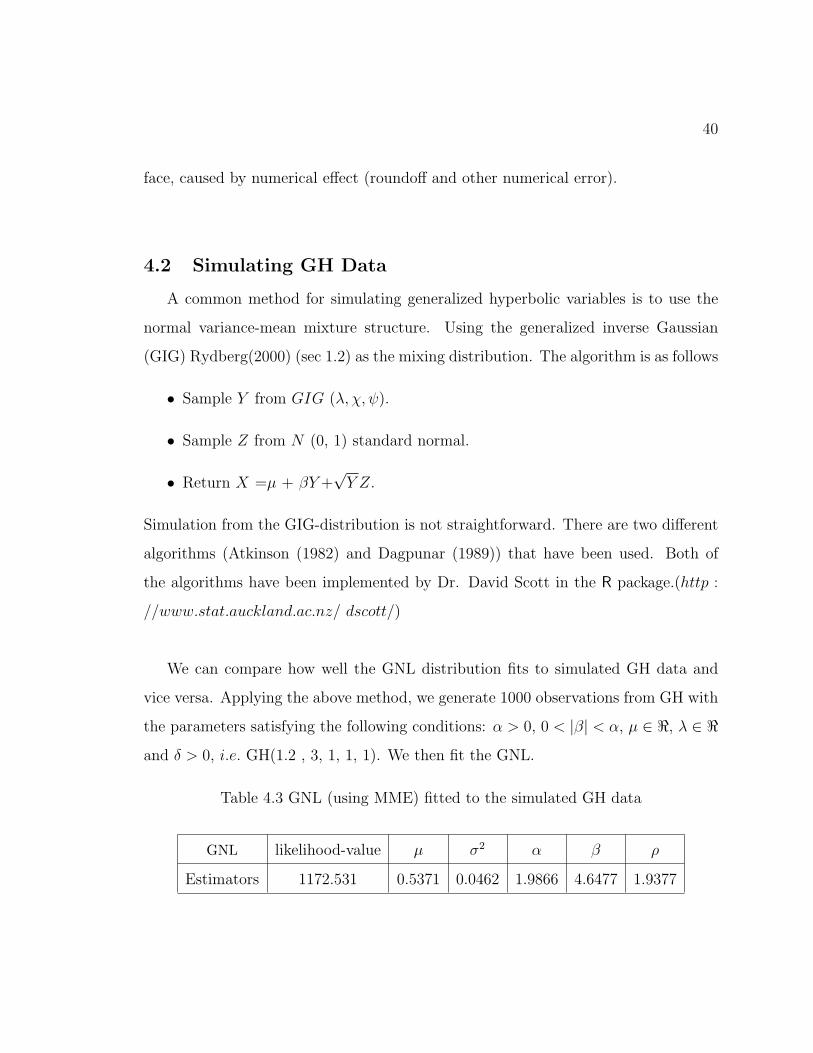
4.2 Simulating GH Data

A common method for simulating generalized hyperbolic variables is to use the

normal variance-mean mixture structure. Using the generalized inverse Gaussian

(GIG) Rydberg(2000) (sec 1.2) as the mixing distribution. The algorithm is as follows

• Sample Y from GIG (λ, χ, ψ).

• Sample Z from N (0, 1) standard normal.

• Return X =µ + βY+√Y Z.

Simulation from the GIG-distribution is not straightforward. There are two different

algorithms (Atkinson (1982) and Dagpunar (1989)) that have been used. Both of

the algorithms have been implemented by Dr. David Scott in the R package.(http :

//www.stat.auckland.ac.nz/ dscott/)

We can compare how well the GNL distribution fits to simulated GH data and

vice versa. Applying the above method, we generate 1000 observations from GH with

the parameters satisfying the following conditions: α > 0, 0 < |β| < α, µ ∈ <, λ ∈ <

and δ > 0, i.e. GH(1.2 , 3, 1, 1, 1). We then fit the GNL.

Table 4.3 GNL (using MME) fitted to the simulated GH data

GNL likelihood-value µ σ2 α β ρ

Estimators 1172.531 0.5371 0.0462 1.9866 4.6477 1.9377

41

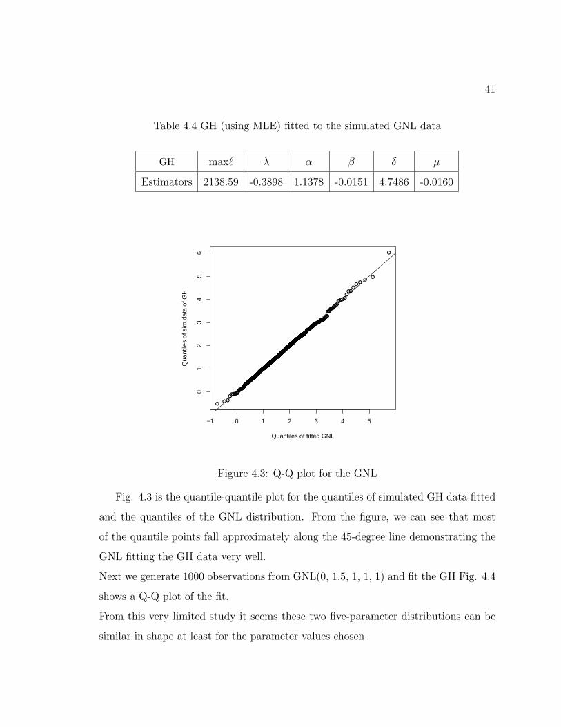
Table 4.4 GH (using MLE) fitted to the simulated GNL data

GH max` λ α β δ µ

Estimators 2138.59 -0.3898 1.1378 -0.0151 4.7486 -0.0160

●●●

●●●●●●●●●●●●●●●●●●●

●●●●●●●●●●●●●●●●●●●●●●●●●●●

●●●●●●●●●●●●●●●●●●●●●●●●●●●●●●●●●●●●●●

●●●●●●●●●●●●●●●●●●●●●●●●●●●●●●●●●●●●●●●●●●●●●●●●●●●●●●●●●●●●●●●●●●●●●●●●●●●●●●●●●●●●●●●●●●●●●●●●●●●●●●●●●●●●●●●●●●●●●●●●●●●●●●●●●●●●●●●●●●●●●●●●●●●

●●●●●●●●●●●●●●●●●●●●●●●●●●●●●●●●●●●●●●●●●●●●●●●●●●●●●●●●●●●●●●●●●●●●●●●●●●●●●●●●●●●●●●●●●●●●●●

●●●●●●●●●●●●●●●●●●●●●●●●●●●●●●●●●●●●●●●●●●●●●●●●●●●●●●●●●●●●●●●●●●●●●●●●●●●●●●●●●●●●●●●●●●●●

●●●●●●●●●●●●●●●●●●●●●●●●●●●●●●●●●●●●●●●●●●●●●●●●●●●●●●●●●●●●●●●●●●●●●●●●●●●●●●●●●●●●●●●●●●●●●●●●●●●●

●●●●●●●●●●●●●●●●●●●●●●●●●●●●●●●●●●●●●●●●●●●●●●●●●●●●●●●●●●●●●●●●●●●●●●●●●●●●●●●●●●●●●●●●●●●●●●●●●●●●●●●●●●●●●●●●●●●●●●●●●●●●●●●●●●●●●●●●●●●●●●●●●●●●●●●●●●●●●●●●●●●●●●●●●●●●●●●●●●●●●●●●●●●●●●●●●●●●●●●●●●●●●●●●●●●●●●●

●●●●●●●●●●●●●●●●●●●●●●●●●●●●●●●●●●●●●●●●●●●●●●●●●●●●●●●●●●●●●●●●●●●●●●●●●●●●●●●●●●●●●●●●●●●●●●●●●●●●●●●●

●●●●●●●●●●●●●●●●●●●●●●●●●●●●●●●●●●●●●●●●●●

●●●●●●●●●●●●●●●●●●●●●●●●●●●●●●●●●●●●●

●●●●●●●●●●●●●●●●●●●●●

●●●●●●●●●●●●●●●●●●●●

●●●●●●●●●●●

●●●●●

●●●●●●●●

●●●●●●

●●●●●

●●

●●

●

●

−1 0 1 2 3 4 5

01

23

45

6


Qua

ntile

s of

sim

.dat

a of

GH

Figure 4.3: Q-Q plot for the GNL

Fig. 4.3 is the quantile-quantile plot for the quantiles of simulated GH data fitted

and the quantiles of the GNL distribution. From the figure, we can see that most

of the quantile points fall approximately along the 45-degree line demonstrating the

GNL fitting the GH data very well.

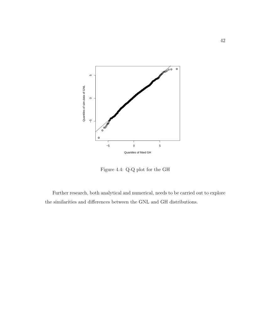
Next we generate 1000 observations from GNL(0, 1.5, 1, 1, 1) and fit the GH Fig. 4.4

shows a Q-Q plot of the fit.

From this very limited study it seems these two five-parameter distributions can be

similar in shape at least for the parameter values chosen.

42

●

●

●●●●●

●●●●●

●●●●●●●●

●●●●●●●●●●●●

●●●●●●●●●●●●●●●●●●●●●●●●●●●●●●●●●●●●●●●●●●●●●●●●●●●●●●●●●●●●●●●●●●●●●●●●●●●●●●●●●●●●●●●●●●●●●●●●●●●●●●●●●●●●●●●●●●●●●●●●●●●●●●●●●●●●●●●●●●●

●●●●●●●●●●●●●●●●●●●●●●●●●●●●●●●●●●●●●●●●●●●●●●●●●●●●

●●●●●●●●●●●●●●●●●●●●●●●●●●●●●●●●●●●●●●●●●●●●●●●●●●●●●●●●●●●●●●●●

●●●●●●●●●●●●●●●●●●●●●●●●●●●●●●●●●●●●●●●●●●●●●●●●●●●●●●●●●●●●●●●●●●●●●●●●●●●●●●●●●●●●●●●●●●●●●●●●●●●●●●●●●●●●●●●●●●●●●●●●●●●●●●●●●●●●●●●●●●●●●●●●●●●●●●●●●●●●●●●●●●●●●●●●●●●●●●●●●●●●●●●●

●●●●●●●●●●●●●●●●●●●●●●●●●●●●●●●●●●●●●●●●●●●●●●●●●●●●●●●●●●●●●●●●●●●●●●●●●●●●●●●●●●●●●●●●●●●●●●●●●●●●●●●●●●●●●●●●●●●●●●●●●●●●●●●●●●●●●●●●●●●●●●●●

●●●●●●●●●●●●●●●●●●●●●●●●●●●●●●●●●●●●●●●●●●●●●●●●●●●●●●●●●●●●●●●●●●●●●●

●●●●●●●●●●●●●●●●●●●●●●●●●●●●●●●●●●●●●●●●●●●●●●●●●●●●●●●●●●●●●●●●●●●●●●●●

●●●●●●●●●●●●●●●●●●●●●●●●●●●●●●●●●●●●●●●●●●●●●●●●●●●●●●

●●●●●●●●●●●●●●●●●●●●●●●●●●●●●●●●●●●●●●●●●●●●●●●●●●●

●●●●●●●●●●●●●●●●●●●●●●●●●●●●●●●●●●●●●●

●●●●●●●●●●●●●●●●●●●●●●●●●●●●●●●●●●

●●●●●●●●●●●●●●●●●●●●●

●●●●●●●●●●●●●●●●

●●●●●●●●●●●●

●●●●●●●

●●●●●●

●● ● ●

−5 0 5

−5

05

Quantiles of fitted GH

Qua

ntile

s of

sim

.dat

a of

GN

L

Figure 4.4: Q-Q plot for the GH

Further research, both analytical and numerical, needs to be carried out to explore

the similarities and differences between the GNL and GH distributions.

Chapter 5

Application to Income Data

This chapter will discuss the application of NL and GNL models and their comparison

against other four and five-parameter models when fitting to grouped income data.

Currently, the generalized beta (GB2) distribution (McDonald, 1984) and the gener-

alized beta or GB (McDonald and Xu, 1995) are being claimed as the best fitting four

and five-parameter models for income data (Bandourian et al., 2002). Consequently,

we compare the performance of the NL with GB2 and of the GNL and GB.

5.1 Description of the Income Data

The household income data are obtained from the Luxembourg Income Study

(LIS) database, including 30 countries from four continents: Europe, Asia, America

and Oceania, and spanning up to 30 years. The term income distribution spans many

kinds of ‘income’ (e.g. earnings is one type of income). Following the LIS definitions

‘earnings’ is the total of gross wages and salaries; total gross income is the sum of

earnings, factor income and market income, and disposable income is the difference

between total gross income and total tax. Only positive earnings data (see table

5.2) are used in this thesis. Hence, if an observation value is equal to or smaller

than zero, it is rejected. Due to privacy laws, income data is considered confidential

information; thus, only grouped income data is available. The samples involve twenty-

equal probability intervals, corresponding to the 5th through 95th percentiles obtained

from the LIS database using a SAS program.

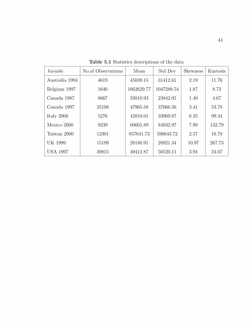
All datasets are in local currency amounts. The following table (Table 5.1) lists the

countries, dates and summary statistics.

44

Table 5.1 Statistics descriptions of the data

Variable No.of Observations Mean Std Dev Skewness Kurtosis

Australia 1994 4619 45039.15 31412.61 2.19 11.76

Belgium 1997 1640 1662629.77 1047288.54 1.87 8.73

Canada 1987 8667 33810.93 23842.05 1.40 4.67

Canada 1997 25108 47965.58 37066.56 3.41 53.78

Italy 2000 5276 42810.01 33969.87 6.35 99.34

Mexico 2000 9239 60601.89 84932.97 7.99 132.79

Taiwan 2000 12301 857641.73 590643.72 2.57 18.79

UK 1999 15199 28180.91 28921.34 10.97 267.73

USA 1997 39815 49412.87 50520.11 3.94 24.07

45

Table 5.2.a Definitions of Income Variables

Define VARIABLE DEFINITION

+ Gross wages and Salaries

+ Farm self-employment income

+ Non-farm self-employment income

= Total Earning

+ Cash property incom

+ Private occupational pensions

+ Public sector pensions

+ Social Retirement benefits

+ Child or family allowances

+ Unemployment compensation

+ Sick pay; Accident pay; Disability pay; Maternity pay

+ Military/vet/war benefits

+ Other social insurance

+ Means-tested cash benefits

+ Near-cash benefits

+ Alimony or Child Support

+ Other regular private income and Other cash income

= Total Gross Income

− Mandatory employee contribution for sled-employed

− Mandatory employee contribution

− Income tax

= Disposable Income

aLuxembourg Income Study website http : //www.lisproject.org

46

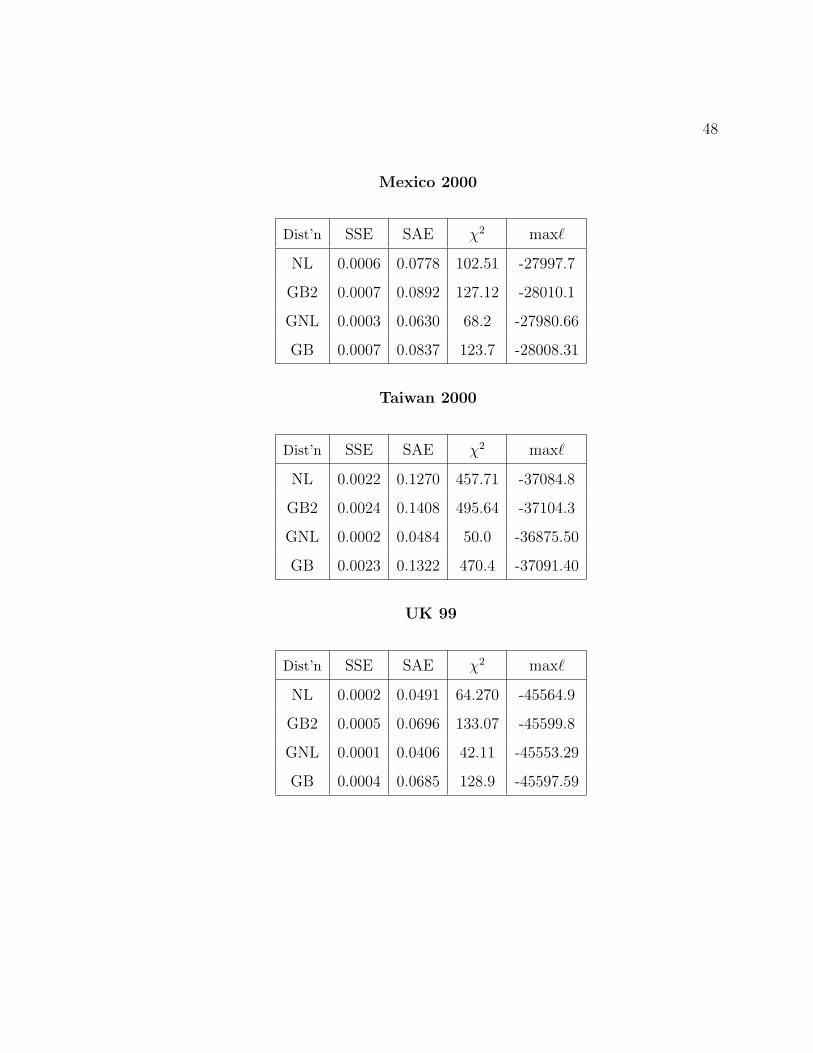
5.2 Income Distribution Results

The following tables contain the goodness-of-fit statistics (the sum of squared er-

rors (SSE), the sum of absolute errors (SAE), the Pearson goodness-of-fit statistic χ2

and the maximized log-likelihood) for the two four-parameter distributions (NL and

GB2), and for the two five-parameter distributions (GNL and GB).

Australia 1994

Dist’n SSE SAE χ2 max`

NL 0.0019 0.1341 151.97 -13914.7

GB2 0.0024 0.1437 195.24 -13936.2

GNL 0.0007 0.0982 66.4 -13869.90

GB 0.0023 0.1353 192.1 -13934.76

Belgium 1997


NL 0.0008 0.1027 47.89 -8729.5

GB2 0.0009 0.1078 54.11 -8732.8

GNL 0.0005 0.0787 29.1 -8720.01

GB 0.0009 0.1096 53.0 -8732.24

47

Canada 1987


NL 0.0007 0.0865 128.90 -26026.4

GB2 0.0010 0.1037 191.17 -26056.6

GNL 0.0004 0.0612 66.8 -25996.47

GB 0.0010 0.1027 189.6 -26055.89

Canada 1997


NL 0.0002 0.0600 118.51 -75275.9

GB2 0.0005 0.0791 228.46 -75330.8

GNL 0.0002 0.04647 84.3 -75258.68

GB 0.0004 0.0757 219.5 -75326.30

Italy 2000


NL 0.0044 0.2345 586.97 -16063.4

GB2 0.0046 0.2418 628.74 -16077.1

GNL 0.0042 0.2233 557.0 -16051.21

GB 0.0046 0.2394 624.7 -16076.45

48

Mexico 2000


NL 0.0006 0.0778 102.51 -27997.7

GB2 0.0007 0.0892 127.12 -28010.1

GNL 0.0003 0.0630 68.2 -27980.66

GB 0.0007 0.0837 123.7 -28008.31

Taiwan 2000


NL 0.0022 0.1270 457.71 -37084.8

GB2 0.0024 0.1408 495.64 -37104.3

GNL 0.0002 0.0484 50.0 -36875.50

GB 0.0023 0.1322 470.4 -37091.40

UK 99


NL 0.0002 0.0491 64.270 -45564.9

GB2 0.0005 0.0696 133.07 -45599.8

GNL 0.0001 0.0406 42.11 -45553.29

GB 0.0004 0.0685 128.9 -45597.59

49

US 97


NL 0.0003 0.0566 266.60 -119406.2

GB2 0.0005 0.0738 418.61 -119480.1

GNL 0.0003 0.0548 218.47 -119384.2

GB 0.0005 0.0719 414.63 -119478.2

In some cases there were multiple local maxima to the log-likelihood function (e.g.

fitting the GNL to Australia 1994, Belgium 1997, Canada 1987, Canada 1997, Taiwan

2000 and UK 1999). However, they resulted in identical values for the maximized log-

likelihood.

While the numerical results for GB2 and GB are comparable to those of Bandourian

et al. (2002), there are some slight differences. These differences may be explained

by one or more of the following reasons: (i) end-point differences - we used 0 and ∞

for the lower and upper boundaries of the smallest and largest class; (ii) differences

in retrieval of data from LIS - we used SAS 9.13; (iii) possibility of multiple local

maxima of the likelihood function for GB2 and GB.

We will discuss the results of NL and GB2 distributions first and subsequently, those

of GNL and GB distributions. As can be seen from the tables, in all cases the

four-parameter NL has better performance than GB2 does; and indeed is better

than the five-parameter GB. The GNL performs notably better than all of the other

distributions. One thing to be emphasized is the nine cases reported are the only ones

to which model fitting was done. They were not selected because the NL and GNL

fitted well. We expect that if the models are fitted to other datasets of Bandourian

et al.(2002), the results would be similar.

Chapter 6

Application To Financial Data

6.1 Description of the Stock Price Data

Empirical studies seem to suggest that the distribution of logarithmic returns tend

to be heavy-tailed. The logarithmic return of a stock is defined as

rt = log(Pt+1)− log(Pt) = log

(Pt+1

Pt

)(6.1)

where Pt is the price of a financial security at time t. To assess the fit of the GNL

distribution to empirical logarithmic returns, and to compare the fit with the GH,

which is now widely used in derivative-pricing models (Eberlein and Hammerstein,

2002) both distributions were fitted to sets of financial data obtained from the website

http : //finance.yahoo.com/. Two sets of data IBM and CitiGroup stock price were

used using a 2-year period, 3 January, 2005 to 29 December, 2006. This resulted in

503 observations in each time series. The adjusted closing price (close price adjusted

for dividends and splits) was used to calculate the logarithmic returns. As discussed

in section 4.1, for large scale parameter ρ of the GNL there is virtually no information

about the tail parameters α and β and also ρ will be confounded with µ and σ2. In

such cases, the likelihood changes very little with the different parameters. Therefore,

MME would be used for the estimation of GNL in this chapter.

6.2 Results of fitting GNL and GH

The following tables show the estimates of GNL and GH when fitted to the log

returns of IBM and CitiGroup stock price, 2005-2006.

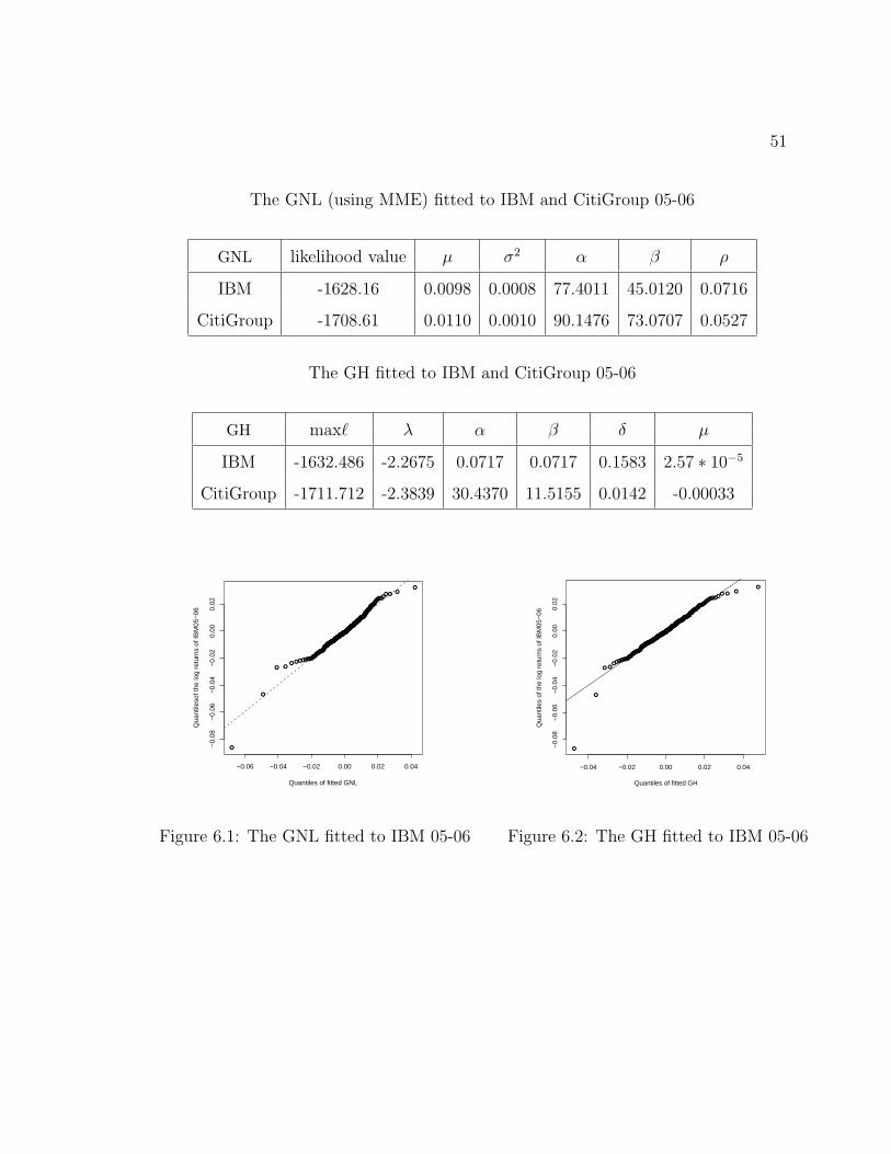
51

The GNL (using MME) fitted to IBM and CitiGroup 05-06

GNL likelihood value µ σ2 α β ρ

IBM -1628.16 0.0098 0.0008 77.4011 45.0120 0.0716

CitiGroup -1708.61 0.0110 0.0010 90.1476 73.0707 0.0527

The GH fitted to IBM and CitiGroup 05-06

GH max` λ α β δ µ

IBM -1632.486 -2.2675 0.0717 0.0717 0.1583 2.57 ∗ 10−5

CitiGroup -1711.712 -2.3839 30.4370 11.5155 0.0142 -0.00033

●

●

● ●● ●●●●●●●●

●●●●●●●●●

●●●●●●●●●●●●●●●●●●●●●●●●●●●

●●●●●●●●●●●●●●●●●●●●●●●●●●●●●●●●●●●●●●●●

●●●●●●●●●●●●●●●●●●●●●●●●●●●●●●●●●●●●●●●●●●●●●●●●●●●●●●●

●●●●●●●●●●●●●●●●●●●●●●●●●●●●●●●●●●●●●●●●●●●●●●●●●●●●●●●●●●●●●●●●●●●●●●●●●●●●●●●●●●●●●

●●●●●●●●●●●●●●●●●●●●●●●●●●●●●●●●●●●●●●●●●●●●●●●●●●●●●●●●●●●●●●●●●●●●●●●●●●●●●●

●●●●●●●●●●●●●●●●●●●●●●●●●●●●●●●●●●●●●●●●●●●●●●●●●●●●●●●●●●

●●●●●●●●●●●●●●●●●●●●●●●●●●●●●●●●●●●●●●●●●●●●●●●●●●●●●●●●

●●●●●●●●●●●●●●●●●●●●●●●●●●●●●●●●●

●●●●●●●●●●●●●●●●●●●●●●●●

●●●●●●●●●●

●●●●●●●●●

●● ●

●●

−0.06 −0.04 −0.02 0.00 0.02 0.04

−0.

08−

0.06

−0.

04−

0.02

0.00

0.02


Qua

ntile

sof t

he lo

g re

turn

s of

IBM

05−

06

Figure 6.1: The GNL fitted to IBM 05-06

●

●

● ●●●●●●●●●●

●●●●●●●●

●●●●●●●●●●●●●●●●

●●●●●●●●●●●●●●●●●●●●●●●

●●●●●●●●●●●●●●●●●●●●●●●●●●●●●●●●●●●●●●●●●●●●●●●●●●●●●

●●●●●●●●●●●●●●●●●●●●●●●●●●●●●●●●●●●●●●●●●●●●●●●●●●●●●●●●●●●●●●●

●●●●●●●●●●●●●●●●●●●●●●●●●●●●●●●●●●●●●●●●●●●●●●●●●●●●●●●●●●●●●●●●●●●●●●●●●●●●●●●●●●●●●●●

●●●●●●●●●●●●●●●●●●●●●●●●●●●●●●●●●●●●●●●●●●●●●●●●●●●●●●●●●●●●●●●●

●●●●●●●●●●●●●●●●●●●●●●●●●●●●●●●●●●●●●●●●●●●●●●●●●●●●●●●●

●●●●●●●●●●●●●●●●●●●●●●●●●●●●●●●●●●●●●●●●●●●●●●

●●●●●●●●●●●●●●●●●●●●●●●●●●●●●●●

●●●●●●●●●●●●●●●●●●

●●●●●●●●●●

●●●●●

●●●●●● ●

●●

−0.04 −0.02 0.00 0.02 0.04

−0.

08−

0.06

−0.

04−

0.02

0.00

0.02


Qua

ntile

s of

the

log

retu

rns

of IB

M05

−06

Figure 6.2: The GH fitted to IBM 05-06

52

●

●●

●●●

●●●●

●●●●●●●●●●●●●●●●●●●●

●●●●●●●●●●●●●●●●●●●●●●

●●●●●●●●●●●●●●●●●●●●●●●●●●●●●●●●●●●●●●●●

●●●●●●●●●●●●●●●●●●●●●●●●●●●●●●●●●●●●●●●●●●●●●●●●●●●●●

●●●●●●●●●●●●●●●●●●●●●●●●●●●●●●●●●●●●●●●●●●●●●●●●●●●●●

●●●●●●●●●●●●●●●●●●●●●●●●●●●●●●●●●●●●●●●●●●●●●●●●●●●●●●●●●●●

●●●●●●●●●●●●●●●●●●●●●●●●●●●●●●●●●●●●●●●●●●●●●●●●●●●●●●●●●●●●●●●●●●

●●●●●●●●●●●●●●●●●●●●●●●●●●●●●●●●●●●●●●●●●●●●●●●●●●●●●●●●●●●●●●●●●●●●●●●●●●●

●●●●●●●●●●●●●●●●●●●●●●●●●●●●●●●●●●●●●●●●●

●●●●●●●●●●●●●●●●●●●●●●●●●●●●●●●●●●●●●●●●●●●●●●●

●●●●●●●●●●

●●● ●●

●

−0.04 −0.02 0.00 0.02

−0.

04−

0.02

0.00

0.02

0.04


Qua

ntile

s of

the

log

retu

rns

of C

itiG

roup

05−

06

Figure 6.3: The GNL fitted to CitiGroup

05-06

●

●●

●●●

●●●●

●●●●●●●●●●●●●●●●●●●●

●●●●●●●●●●●●●●●●●●●●●●

●●●●●●●●●●●●●●●●●●●●●●●●●●●●●●●●●●●●●●●●

●●●●●●●●●●●●●●●●●●●●●●●●●●●●●●●●●●●●●●●●●●●●●●●●●●●●●

●●●●●●●●●●●●●●●●●●●●●●●●●●●●●●●●●●●●●●●●●●●●●●●●●●●●●●●●●●●●●●●●●●●●●●●●●●●●●●●●●●●●●●●

●●●●●●●●●●●●●●●●●●●●●●●●●●●●●●●●●●●●●●●●●●●●●●●●●●●●●●●●●●●●

●●●●●●●●●●●●●●●●●●●●●●●●●●●●●●●●●●●●●●●●●●●●●●●●●●●●●●●●●●●●●●●

●●●●●●●●●●●●●●●●●●●●●●●●●●●●●●●●●●●●●●●●●●●

●●●●●●●●●●●●●●●●●●●●●●●●●●●●●●●●●●●●●●●●●

●●●●●●●●●●●●●●●●●●●●●●●●●●●●●

●●●●●●●●●●

●●●●●●●●

●●●●●●●●●●

●● ● ●●

●

−0.02 0.00 0.02 0.04

−0.

04−

0.02

0.00

0.02

0.04


Qua

ntile

s of

the

log

retu

rns

of C

itiG

roup

05−

06

Figure 6.4: The GH fitted to CitiGroup

05-06

Q-Q plots for fitting the GNL and GH to IBM 2005-2006 indicate that neither fit

very well in the lower tail; For the CitiGroup 2005-2006, the Q-Q plot for the GNL

appears more satisfactory than for the GH. Also, calculated after estimating by MME,

the log-likelihood values for IBM and Citigoup 2005-2006 for the GNL distribution are

smaller than the maximum log-likelihood values for the GH. As known, the MLE is a

better estimation than the MME. If we can solve the MLE multiple maxima problem

for the GNL distribution, then we should get smaller maximum log-likelihood value

which it would be an even better result than the GH. While the fits of neither the

GH nor the GNL are perfect, the results suggest that the fit of the GNL is at least

as good as for the more well-known GH.

Chapter 7

Conclusions

Two families of heavy-tailed distributions: the normal-Laplace (NL) and its relative

distribution the generalized normal-Laplace (GNL) distribution are the focus of this

thesis. We have summarized the major properties of the GNL and NL distributions.

The thesis gives prominence to parameter estimation for the five-parameter GNL and

four-parameter NL distributions to grouped income data by maximum likelihood.

The results of fitting four theoretical distributions to nine income datasets clearly

indicate that the NL fits better than what has previously been claimed as the best-

fitting four-parameter model for income distribution namely the GB2 (McDonald,

1984). Indeed it fits better than what has been previously claimed as the best fitting

five-parameter distribution the GB (McDonald and Xu, 1995). The five-parameter

GNL distribution provides an even better fit.

Even though there are no closed form expressions for the pdf and cdf of the

GNL, they can be obtained numerically from the convolution of GL and Normal dis-

tributions. However, ML estimation for the GNL is not always satisfactory, there

sometimes being problems with multiple maxima. Furthermore it requires consider-

able computing time.

The similarity of the GNL and GH distribution was demonstrated using simula-

tion in which in turn the GNL and GH were fitted to samples generated from the

other. Also the two models were fitted to two-year log returns of IBM and CitiGroup

stock prices and the results indicate that GNL and GH distributions provide similar

54

good fits to the data. These results suggest that the GNL may provide a model

at least as good as the more widely known GH for fitting to financial data. Op-

tion pricing for European call options for assets following Brownian-Laplace motion,

whose increments have a GNL distribution, has been developed by Reed (2007). More

work in this area could lead to the GNL providing a viable alternative to the GH in

option-pricing theory. However some difficulties remain mainly to do with maximum

likelihood estimation of the GNL parameters.

As we have discussed in this thesis, since there is no closed-form for the pdf

or cdf of th GNL distribution, evaluating the likelihood function involves numerical

integration for each data point whichever of three methods is used. This makes

numerical maximization of the likelihood function rather slow. In addition there

appear to be problems with flat likelihoods and multiple maximum, especially when

the parameters α, β and ρ are large. The application in this thesis is a beginning

of research in fitting the GNL and its family. We have some other areas for further

research:

• More work on ML estimation of the GNL distribution for ungrouped data.

• Using methods such as the EM algorithm for fitting GNL distribution.

• Using analytic and numerical methods for finding similarities and differences

between the GNL and GH distributions.

• The application of the GNL to credit risk, risk management and portfolio opti-

mization problems as has been conducted using the GH distribution.

References

Abramowitz, M. and Stegun, I.A., 1972. Handbook of Mathematical Functions.

Dover Publications, New York.

Aitchinson, J., and Brown, J.A.C., 1969. The lognormal distribution with

special reference to its uses in economics, Cambridge University Press.

Ammon, O., 1895. Die Gesellschaftsordnung und ihre Naturlichen Grundlagen,

Jena.

Amoroso, L. , 1924-1925. Ricerche Intorno alla Curva dei Redditi, Annali di

Matematica. Pura ed Applicata, Series 4-21.2:123-157.

Atkinson, A. C., 1982. The simulation of generalized inverse gaussian and hyper-

bolic random variables. SIAM Journal of Scientific & Statistical Computing, 3:502-

515.

Bandourian, R., McDonald, J. B. and Turley, R. S., 2002. A comparison of

parametric models of income distribution across countries and over time. Luxembourg

Income Study Working Paper, No. 305.

Barndorff-Nielsen,O., 1977. Exponentially decreasing distributions for the log-

arithm of particle size, Proceedings of the Royal Society of London A 353 (1977),

401-419.

Barndorff-Nielsen, O., Kent J. and Srensen, M., 1982. Normal Variance-Mean

Mixtures and z Distributions. International Statistical Review, 50, 145-159.

Blsild, P and Srensen, M.K., 1992. ’Hyp’ - A computer program for analyzing by

means of the hyperbolic distribution. Department of Theoretical Statistics, Research

Report No.300.

56

Bartels, C.P.A. and van Metelen, H., 1975. Alternative Probability Density

Functions of Income, Vrije University Amerstadam: Research memorandum 29, 30

pages.

Burr,I. W., 1942. Cumulative frequency functions. Ann. Math. Statist. 13,

215-32.

Carr, P., H. Geman, D. Madan and M. Yor, 2002. The Fine Structure of

Asset Returns: An Empirical Investigation, Journal of Business, 75,305-332.

Chhikara, R. S. and Folks, J. L., 1989. The Inverse Gaussian Distribution, New

York: Dekker.

Kleiber,Carlos, 1996. Dagum vs. Singh-Maddala income distributions. Economics

Letters, 53, 265-268.

Dastrup, S.R., McDonald, J. B. and Hartshorn, Rachel, 2005. The Im-

pact of Taxes and Transfer Payments on the Distribution of Income: a Parametric

Comparison. Luxembourg Income Study Working Paper, No. 401.

Dagum, C., 1977. A new model for personal income distribution: specification and

estimation. Economie Applique, 30, 413-437.

Dagum, C., 1980. The generation and distribution of income, the Lorenz curve

and the Gini ratio. Economie Appliqu e, 33, 327-367.

Dagpunar,J. S., 1989. An easily implemented generalized inverse gaussian gener-

ator. Communications in Statistics, Simulations 18:703C71

Eberlein, E. and Hammerstein, Ernst August v., 2002. Generalized Hy-

perbolic and Inverse Gaussian Distributions: Limiting Cases and Approximation of

Processes, University of Freiburg.

Eberlein, E. and U. Keller, 1995. Hyperbolic distributions in finance. Bernoulli,

1, 281-299.

57

Gibrat, R., 1931. Les Inegalites Economiques. Sirely, Paris.

Cvitanic, Jaksa and Zapatero, Fernando, 2004. Introduction to the Economics

and Mathematics of Financial Markets. Cambridge Massachusetts: MIT Press.

Kleiber, Christian, 1996. Dagum vs. Singh-Maddala income distributions. Eco-

nomics Letters, 53, 265-268.

Knight, John and Satchell, Stephen, 2001. Return Distributions in Finance,

285-293.

Kotz, S., T. J. Kozubowski and K. Podgorski, 2001. The Laplace Distribution

and Generalizations. Birkhauser, Boston.

Madan, Dilip, and Seneta, Eugene, 1990. The V.G. Model for Share Returns.

Journal of Business, 63, 511-524.

McDonald, J.B. and Ransom, Michael R., 1979. Functional Forms, Estimation

Techniques and the Distribution of Income. Econometrica, Vol 47, 1513-1526.

McDonald, J.B., 1984. Some generalized functions for the size distribution of

income. Econometrica, 52, 647-663.

McDonald, J.B. and Xu, Y. J., 1995. A generalization of the beta distribution

with applications. Journal of Econometrics, 66, 133-152.

Nelder, J. A. and Mead, R., 1965. A Simplex Method for Function Minimization.

Computer Journal, 7, 308-313.

Pareto, V. 1895. ”La Legge della Domanda”, Giornale degli Economisti, Gennaio:59-

68.

Reed, W. J., 2003. The Pareto law of incomes - an explanation and an extension.

Physica A, 319, 579-597.

58

Reed, W. J., 2004. The Normal-Laplace Distribution and its Relatives. In Order

Statistics and Inference, N.Balakrishna etal. (eds)Birkhauser.

Reed, W. J., 2007. Brownian-Laplace motion and its use in financial modelling.

Commun. Stat. - Theory & Methods, 36, 473:484.

Reed, W. J. and M. Jorgensen, 2004. The double Pareto-lognormal distribution

- A new parametric model for size distribution. Commun. Stat. - Theory & Methods,

33, 1733-1753

Rydberg, Tina Hviid, 2000. Realistic Statistical Modelling of Financial Data. J.

Nuffld College, Oxford, United Kingdom.

Seshadri, V., 1993. The Inverse Gaussian Distribution. Clarendon Press.

Singh, S,K, and G.S, Maddala, 1976. A function for the size distribution of

income. Econometrica, 44, 963-970.

Shephard, N.G., 1991. From Characteristic Functions to Distribution Function:

A Simple Framework For The Theory. Cambridge University Press.

Schoutens, W. and Teugels, J.L. 1998. Levy processes, polynomials and mar-

tingales. Communications in Statistics - Stochastic Models, 14, 335-349.

Taille, C., Patil, G.P and Balderssari, B., 1981. Ordering within the Gener-

alized Gamma Family of Income Distributions. Statistical Distributions in Scientific

Work, Vol 6.

Thurow, L.C., 1970. Analyzing the American Income Distribution. American

Economics Association, 60, 261-269

Waller, Lance A., Turnbull, Bruce W. and Hardin, J. Michael, 1995. Ob-

taining Distribution Functions by Numerical Inversion of Characteristic Functions

With Application. The American Statistican, Vol 49., No.4.

59

Wolff, Sebastian, 2004. A local and globalized, constrained and simple bounded

Nelder-Mead method.

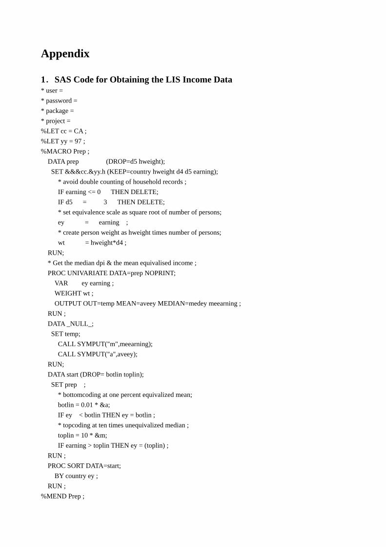
Appendix 1．SAS Code for Obtaining the LIS Income Data * user = * password = * package = * project = %LET cc = CA ; %LET yy = 97 ; %MACRO Prep ; DATA prep (DROP=d5 hweight); SET &&&cc.&yy.h (KEEP=country hweight d4 d5 earning); * avoid double counting of household records ; IF earning <= 0 THEN DELETE; IF d5 = 3 THEN DELETE; * set equivalence scale as square root of number of persons; ey = earning ; * create person weight as hweight times number of persons; wt = hweight*d4 ; RUN; * Get the median dpi & the mean equivalised income ; PROC UNIVARIATE DATA=prep NOPRINT; VAR ey earning ; WEIGHT wt ; OUTPUT OUT=temp MEAN=aveey MEDIAN=medey meearning ; RUN ; DATA _NULL_; SET temp; CALL SYMPUT("m",meearning); CALL SYMPUT("a",aveey); RUN; DATA start (DROP= botlin toplin); SET prep ; * bottomcoding at one percent equivalized mean; botlin = 0.01 * &a; IF ey < botlin THEN ey = botlin ; * topcoding at ten times unequivalized median ; toplin = 10 * &m; IF earning > toplin THEN ey = (toplin) ; RUN ; PROC SORT DATA=start; BY country ey ; RUN ; %MEND Prep ;

61

%MACRO quantile ; PROC UNIVARIATE DATA=start NOPRINT; BY country ; VAR ey ; WEIGHT wt ; OUTPUT OUT = tmp PCTLPTS = 5 to 95 by 5 PCTLPRE = dec ; RUN ; DATA &cc.&yy._2 (KEEP=country d5 d10 d15 d20 d25 d30 d35 d40 d45) ; MERGE start (KEEP=country) tmp ; d5 = dec5 ; d10 = dec10; d15 = dec15; d20 = dec20; d25 = dec25; d30 = dec30; d35 = dec35; d40 = dec40; d45 = dec45; IF _N_ = 1 ; RUN; %MEND quantile ; %MACRO tabulate ; PROC TABULATE DATA=&dataset FORMAT=&formgen FORMCHAR=&bordure NOSEPS; CLASS &classe ; VAR &variable ; TABLE &table / CONDENSE PRINTMISS BOX="&box" RTS=&rts ; KEYLABEL &lab ; RUN ; %MEND tabulate ; %MACRO show ; DATA &cc.&yy._KF ; MERGE &cc.&yy._2; BY country ; ATTRIB d5 label='P5' format=10.4

62

d10 label='P10' format=10.4 d15 label='P15' format=10.4 d20 label='P20' format=10.4 d25 label='P25' format=10.4 d30 label='P30' format=10.4 d35 label='P35' format=10.4 d40 label='P40' format=10.4 d45 label='P45' format=10.4 ; RUN ; %LET dataset= &cc.&yy._2 ; %LET formgen = 15.4 ; %LET bordure = '|---|+|---|+|---|+|---|---|+|---|+|---|+|---+' ; %LET classe = country ; %LET variable = d5 d10 d15 d20 d25 d30 d35 d40 d45 ; %LET table = country, d5 d10 d15 d20 d25 d30 d35 d40 d45; %LET box = 'Percentile ' ; %LET rts = 40 ; %LET lab = sum = ' ' ; %TABULATE %MEND show ; &&&cc.&yy.f ; %PREP %QUANTILE %SHOW

63

R code for numerically computing the pdf of GNL 2．Using the Representation as a Convolution # PDF of gen. Laplace GL.pdf<-function (x,alpha,beta,tau) {# PDF of gen. laplace in terms of my parameters (Kotz et al., p. 189) l.box1<-(tau/2+1/4)*log(alpha*beta)+(beta-alpha)*x/2 l.box1<-l.box1-lgamma(tau)-log(pi)/2 -(tau/2-1/4)*log(2) box1<-exp(l.box1) l.box2<-(tau-1/2)*(log(2*alpha*beta)/2 +log(abs(x))-log(alpha+beta)) l.box3<-log(besselK(abs(x)*(alpha+beta)/2,abs(tau-1/2),expon.scaled =TRUE))-abs(x)*(alpha+beta)/2 box2.3<-ifelse(tau>0.5,(1/2)*gamma(tau-1/2)*(4*sqrt(2*alpha*beta)*(alpha+beta)^(-2))^(tau-1/2) ,gamma(0.5-tau)*2^(-2*tau)*(sqrt(2*alpha*beta))^(tau-0.5)*(abs(x))^(2*tau-1)) box0<-box1*box2.3 out<-ifelse(x==0,box0,exp(l.box1+l.box2+l.box3)) ifelse(is.finite(out)==TRUE,out,1e8)} # CDF of gen Laplace GL.cdf<-function (x,alpha,beta,tau) { int.fn<-function (y)

{ sapply(y,FUN=GL.pdf,alpha=alpha,beta=beta,tau=tau)} temp1<-ifelse(x<0,integrate(int.fn,low=-Inf,upp=x,rel.tol =1e-10,abs.tol = 1e-10)$value,integrate(int.fn,low=-Inf,upp=0)$value+integrate(int.fn,low=0,upp=x,rel.tol =1e-10,abs.tol = 1e-10)$value) temp1} # CDF of GNL Convolution Form GNL.cdf<-function (x,mu,sigma2,alpha,beta,rho) { # Computes cdf of GNL by convolution of GL and normal sigma<-sqrt(sigma2) temp.fn<-function(t){ out<-GL.pdf(t,alpha,beta,rho)*pnorm(x-t,mu*rho,sqrt(sigma2*rho)) out } int.fn<-function(y) sapply(y,FUN=temp.fn) temp1<-integrate(int.fn,lower=-Inf,upper=0,stop.on.error=F,rel.tol =1e-10, abs.tol = 1e-10,subdivisions=100000) temp2<-integrate(int.fn,lower=0,upper=Inf,stop.on.error=F,rel.tol =1e-10, abs.tol = 1e-10,subdivisions=100000) temp1$value + temp2$value }

64

# PDF of GNL Convolution Form GNL.pdf<-function (x,mu,sigma2,alpha,beta,rho) {# Computes pdf of GNL by convolution of GL and normal sigma<-sqrt(sigma2) temp.fn<-function(t){ out<-GL.pdf(t,alpha,beta,rho)*dnorm(x-t,mu*rho,sqrt(sigma2*rho)) out } int.fn<-function(y) sapply(y,FUN=temp.fn) temp1<-integrate(int.fn,lower=-Inf,upper=0,stop.on.error=F,rel.tol =1e-8, abs.tol = 1e-8,subdivisions=100000) temp2<-integrate(int.fn,lower=0,upper=Inf,stop.on.error=F,rel.tol =1e-8, abs.tol = 1e-8,subdivisions=100000) temp1<-ifelse(temp1$message=="OK",temp1$value,1e4) temp2<-ifelse(temp2$message=="OK",temp2$value,1e4) temp1 + temp2} #Income log-Likelyhood Function## llik.GNL.grouped<-function(par,groupdata) {# Log-lik. for fitting GNL to " Grouped data" interval<-log(groupdata[,1]) freq<-groupdata[,2] mu<-par[1] sigma2<-par[2] alpha<-par[3] beta<-par[4] rho<-par[5] prob<-numeric(length(interval)) prob[1]<-GNL.cdf(interval[1],mu=mu,sigma2=sigma2,alpha=alpha,beta=beta,rho=rho)-GNL.cdf(0,mu=mu,sigma2=sigma2,alpha=alpha,beta=beta,rho=rho) for(i in 2:length(interval)){ if(i ==length(interval)) prob[length(interval)]<-1-sum(prob[1:length(interval)-1]) else prob[i]<-GNL.cdf(interval[i],mu=mu,sigma2=sigma2,alpha=alpha,beta=beta,rho=rho)-GNL.cdf(interval[i-1],mu=mu,sigma2=sigma2,alpha=alpha,beta=beta,rho=rho) } sum(log(prob)*freq)} obj.GNL.grouped<-function(par,groupdata) {-llik.GNL.grouped(par,groupdata) } obj.GNL.grouped.new<-function(par,groupdata) { # sigma^2, alpha, beta, rho >0, mu real # par.new<-c(par[1],par[2]^2,par[3]^2,par[4]^2,par[5]^2) obj.GNL.grouped(par.new,groupdata) }

65

3．Inversion of Characteristic Function and Normal Mean-variance Mixture #PDF and CDF of the GNL: Numerical Inversion of Characteristic Function GNL.pdf.in<-function (x,mu,sigma2,alpha,beta,rho){ y<-x-rho*mu cf.fn<-function(s){ cplex<-complex(1,0,1) temp1<-alpha*beta*exp(-sigma2*s^2/2) temp2<-(alpha-cplex*s)*(beta+cplex*s) out<-(temp1/temp2)^rho out} temp.fn<-function(s){ (Mod(cf.fn(s)))*cos(Arg(cf.fn(s))-s*y)} int.fn<-function(t){sapply(t,FUN=temp.fn)} te<-integrate(int.fn,lower=0,upper=Inf,rel.tol=1e-10,subdivisions=1000000) temp3<-ifelse(te$message=="OK", te$value/pi,NA) temp3 } GNL.cdf.in<-function (x,mu,sigma2,alpha,beta,rho){ y<-x-rho*mu #c.f. for mu=0 GNL cf.fn<-function(s){ cplex<-complex(1,0,1) temp1<-alpha*beta*exp(-sigma2*s^2/2) temp2<-(alpha-cplex*s)*(beta+cplex*s) out<-(temp1/temp2)^rho out} temp.fn<-function(s){ (Mod(cf.fn(s))/(s*pi))*sin(s*y-Arg(cf.fn(s)))} int.fn<-function(t){sapply(t,FUN=temp.fn)} te<-integrate(int.fn,lower=0,upper=Inf,rel.tol =1e-10,subdivisions=1000000) temp3<-ifelse(te$message=="OK", te$value,1e4) temp3+0.5 } #PDF for the GNL: Normal mean-variance mixture GNL.pdf.NV<-function (x,mu,sigma2,alpha,beta,rho){ temp.fn<-function(t0){ out<-dnorm(x,mu+(1/alpha-1/beta)*t0,sqrt(sigma2+ t0*(2/(alpha*beta))),log=T)+dgamma(t0,shape=rho,rate=1,scale=1,log=T) exp(out)} int.fn<-function(y) sapply(y,FUN=temp.fn)

66

temp1<-integrate(int.fn,lower=0,upper=Inf,rel.tol=1e-8,abs.tol=1e-8,subdivisions=100000) temp1$value } #Ungrouped Data- log-Likelyhood Function## llik.GNL<-function(par,data) {# Log-lik. for fitting GNL to "data" mu<-par[1] sigma2<-par[2] alpha<-par[3] beta<-par[4] rho<-par[5] temp<-sapply(data,FUN=GNL.pdf,mu=mu,sigma2=sigma2,alpha=alpha,beta=beta,rho=rho) sum(log(temp))} obj.GNL<-function(par,data) { -llik.GNL(par,data)} obj.1.GNL<-function(par,data) { # neg. log.lik using pars. sqrt(sigma2),sqrt(alpha) etc. par.1<-c(par[1],par[2]^2,par[3]^2,par[4]^2,par[5]^2) obj.GNL(par.1,data)} # Equation for computing p-quantile of GNL quant.GNL.eq<-function(x,p,mu,sigma2,alpha,beta,rho) {# Equation defining p-quantile of GNL GNL.cdf(x,mu,sigma2,alpha,beta,rho) - p } ##### for one P-quantile only### quant.1.GNL<- function(p,mu,sigma2,alpha,beta,rho) {out<-uniroot(quant.GNL.eq,low=-100,upp=100,p=p,mu=mu,sigma2=sigma2,alpha=alpha,beta=beta,rho=rho,tol=1e-9) ifelse(out$f.root>-5,out$root,0) } #### for a vector of P-quantiles#### quant.all.GNL<-function(p.vr,mu,sigma2,alpha,beta,rho) {sapply(p.vr,FUN=quant.1.GNL,mu=mu,sigma2=sigma2,alpha=alpha,beta=beta,rho=rho) } #NL cdf## NL.cdf<-function(x,mu,sigma2,alpha,beta){ sigma<-sqrt(sigma2) temp1<-pnorm((x-mu)/sigma) temp2<-(beta*millsratio(alpha*sigma-(x-mu)/sigma)-alpha*millsratio(beta*sigma+(x-mu)/sigma))/(alpha+beta) temp3<-dnorm((x-mu)/sigma)*temp2 temp1-temp3}

Applications of The Normal Laplace and Generalized Normal ...

Documents

Transcript of Applications of The Normal Laplace and Generalized Normal ...