APPLICATIONS OF REVENUE MANAGEMENT IN...
107
APPLICATIONS OF REVENUE MANAGEMENT IN HEALTHCARE by Alia Stanciu BBA, Romanian Academy for Economic Studies, 1999 MBA, James Madison University, 2002 Submitted to the Graduate Faculty of Joseph M. Katz Graduate School of Business in partial fulfillment of the requirements for the degree of Doctor of Philosophy University of Pittsburgh 2009
Transcript of APPLICATIONS OF REVENUE MANAGEMENT IN...

APPLICATIONS OF REVENUE MANAGEMENT IN HEALTHCARE
by
Alia Stanciu
BBA, Romanian Academy for Economic Studies, 1999
MBA, James Madison University, 2002
Submitted to the Graduate Faculty of
Joseph M. Katz Graduate School of Business in partial fulfillment
of the requirements for the degree of
Doctor of Philosophy
University of Pittsburgh
2009

ii
UNIVERSITY OF PITTSBURGH
JOSEPH M. KATZ GRADUATE SCHOOL OF BUSINESS
This dissertation was presented
by
Alia Stanciu
It was defended on
July 8th
, 2009
and approved by
Jerrold H. May, Professor, Business Administration
Jennifer Shang, Associate Professor, Business Administration
David Strum, Associate Professor, Anesthesiology
Pandu Tadikamalla, Professor, Business Administration
Dissertation Advisor: Luis G. Vargas, Professor, Business Administration

iii
Copyright © by Alia Stanciu
2009
iv
Most profit oriented organizations are constantly striving to improve their revenues while
keeping costs under control, in a continuous effort to meet customers‟ demand. After its proven
success in the airline industry, the revenue management approach is implemented today in many
industries and organizations that face the challenge of satisfying customers‟ uncertain demand
with a relatively fixed amount of resources (Talluri and Van Ryzin 2004). Revenue management
has the potential to complement existing scheduling and pricing policies, and help organizations
reach important improvements in profitability through a better management of capacity and
demand.
The work presented in this thesis investigates the use of revenue management techniques
in the service sector, when demand for service arrives from several competing customer classes
and the amount of resource required to provide service for each customer is stochastic. We look
into efficiently allocating a limited resource (i.e., time) among requests for service when facing
variable resource usage per request, by deciding on the amount of resource to be protected for
each customer and surgery class. The capacity allocation policies we develop lead to
maximizing the organization‟s expected revenue over the planning horizon, while making no
assumption about the order of customers‟ arrival. After the development of the theory in Chapter
3, we show how the mathematical model works by implementing it in the healthcare industry,
more specifically in the operating room area, towards protecting time for elective procedures and
APPLICATIONS OF REVENUE MANAGEMENT IN HEALTHCARE
Alia Stanciu, PhD
University of Pittsburgh, 2009

v
patient classes. By doing this, we develop advance patient scheduling and capacity allocation
policies and apply them to scheduling situations faced by operating rooms to determine optimal
time allocations for various types of surgical procedures.
The main contribution is the development of the methodology to handle random resource
utilization in the context of revenue management, with focus in healthcare. We also develop a
heuristics which could be used for larger size problems. We show how the optimal and heuristic-
based solutions apply to real-life situations. Both the model and the heuristic find applications in
healthcare where demand for service arrives randomly over time from various customer
segments, and requires uncertain resource usage per request.
vi
TABLE OF CONTENTS
ACKNOWLEDGMENTS .......................................................................................................... XI
1.0 INTRODUCTION ........................................................................................................ 1
1.1 DISSERTATION OVERVIEW ......................................................................... 1
1.2 PROBLEM STATEMENT ................................................................................. 4
1.3 RESEARCH CONTRIBUTIONS ...................................................................... 6
1.4 SUMMARY OF CHAPTERS ............................................................................. 7
2.0 LITERATURE REVIEW ............................................................................................ 8
2.1 REVENUE MANAGEMENT............................................................................. 8
2.1.1 Forecasting ..................................................................................................... 11
2.1.2 Capacity allocation/seat inventory control .................................................. 12
2.1.3 Overbooking ................................................................................................... 19
2.2 HEALTHCARE ................................................................................................. 20
2.3 MAPPING REVENUE MANAGEMENT CONCEPTS TO THE
HEALTHCARE ENVIRONMENT ................................................................................... 26
3.0 MODELING THE PROBLEM OF CAPACITY ALLOCATION UNDER
VARIABLE SERVICE TIME ASSUMPTION ....................................................................... 33
3.1 DETERMINISTIC CASE ................................................................................. 34
3.2 RANDOM RESOURCE REQUIREMENTS .................................................. 35

vii
3.3 EXTENSION TO MULTIPLE CLASSES ...................................................... 39
4.0 REVENUE MANAGEMENT WITH RANDOM RESOURCE
REQUIREMENTS: APPLICATIONS IN HEALTHCARE .................................................. 47
4.1 PROBLEM SETTING OVERVIEW ............................................................... 48
4.2 HEALTHCARE APPLICATION - MOTIVATION ..................................... 51
4.3 PROBLEM STATEMENT IN THE OPERATING ROOM SETTING ...... 53
4.4 DATA SUMMARY ............................................................................................ 55
4.5 RANDOM RESOURCE REQUIREMENTS: APPLICATION RESULTS 58
4.5.1 Case 1 .............................................................................................................. 61
4.5.1.1 Two Classes .......................................................................................... 61
4.5.1.2 Multiple classes .................................................................................... 64
4.5.2 Case 2 .............................................................................................................. 68
4.5.2.1 Two classes ........................................................................................... 68
4.5.2.2 Three classes ........................................................................................ 71
4.5.2.3 Multiple classes .................................................................................... 72
4.5.3 Conclusions and revenue results .................................................................. 73
4.6 PROBLEM COMPLEXITY............................................................................. 74
4.7 HEURISTIC SOLUTION ................................................................................. 75
4.7.1 Heuristic implementation and solution........................................................ 78
4.7.2 Heuristic application: an extension .............................................................. 80
5.0 CONCLUSIONS AND FUTURE RESEARCH ...................................................... 84
5.1 SUMMARY ........................................................................................................ 84
5.2 MODEL EXTENSIONS ................................................................................... 86
viii
5.2.1 Deciding the number of patients to accept .................................................. 86
5.2.2 Forecasting demand and deciding on the length of the booking period ... 87
5.2.3 Deciding how many operating rooms to open ............................................. 88
5.3 FUTURE STUDIES ........................................................................................... 89
5.3.1 Dynamic programming and the time value of money ................................ 89
5.3.2 Discount/premium policies for postponement/faster service options ....... 89
5.3.3 Accounting for Emergencies ......................................................................... 90
5.3.4 Advance booking system, cancellations and no shows ............................... 90
BIBLIOGRAPHY ....................................................................................................................... 91

ix
LIST OF TABLES
Table 1: Subspecialty nomenclature ............................................................................................. 56
Table 2: Surgical data description................................................................................................. 57
Table 3: Protection levels in Case 1 with 18 classes. ................................................................... 66
Table 4: Protection levels in Case 2 with 4 classes. ..................................................................... 73
Table 5: Protection levels in Case 2 with 6 classes. ..................................................................... 73
Table 6: Protection levels comparison (x and x*) for 4 and 6 classes .......................................... 78
Table 7: Protection levels comparison (x and x*) for 9 classes .................................................... 79
x
LIST OF FIGURES
Figure 1: Relation between protection level x1, booking limits b1 and b2, and capacity .............. 14
Figure 2: Tradeoff between spoilage and dilution ........................................................................ 15
Figure 3: Case 1, Example 1 – Protection levels and Expected Total Revenue ........................... 62
Figure 4: Case 1, Example 2 – Protection levels and Expected Total Revenue ........................... 63
Figure 5: Case 1, Example 3 – Protection levels and Expected Total Revenue ........................... 64
Figure 6: Comparison of optimal protection levels per class and per CPT function of capacity . 67
Figure 7: Case 2, Example 1 – Protection levels and Expected Total Revenue ........................... 68
Figure 8: Case 2, Example 2 - Optimal vs. simulation-based protection levels ........................... 69
Figure 9: 3D Plot of (6) for Case 2 with 3 classes ........................................................................ 72
Figure 10: Protection levels comparison (x and x*) for 4 and 6 classes ....................................... 78
Figure 11: Protection levels comparison for 9 classes .................................................................. 80
Figure 12: Distribution of protection levels for 9 classes ............................................................. 82

xi
ACKNOWLEDGMENTS
Writing this thesis, with all the hurdles it entailed, was an integral part of my life as a
Ph.D. candidate at Katz Graduate School of Business. This accomplishment, one of the greatest
in my life, wouldn‟t have been possible without the guidance and support of several key people
whom I admire, from both my professional and personal life.
My deepest gratitude goes to my advisor, Dr. Luis Vargas, for all the intellectual and
moral support and guidance he provided, and for all the great ideas he ran by me over the years,
most of which either became part of this work, or about to be incorporated in other research
projects. This work wouldn‟t have seen the light of day if it weren‟t for him. Luis, thank you!
Special thanks go to Dr. Jerry May, whose pieces of advice I‟ll always cherish. Dr. May,
with his unique way of approaching things, on both professional and personal levels, always
provided insightful ideas and lifted my confidence in me and my work when problems were
daunting me. Thank you for the delicious apple strudels you brought to most research meetings,
which complemented the hot topics we were discussing and helped spurring new ones.
Many thanks go to Dr. Jennifer Shang and Dr. Pandu Tadikamalla for keeping an open
eye over my progress, and for their support when needed. I am extremely grateful for the support
of Dr. David Strum, who guided me from afar, and who provided me with very useful insights
and suggestions that helped me move forward with my research. I am a better researcher and
teacher because of the five great minds mentioned above. But I am still sane and I was able to
stay on track due to the constant help and advice from the amazing people in the doctoral office,
especially Carrie. Thank you! You all became my second family while I was at Katz!
I am dedicating this work to my husband, Mihai Banciu, who was in this with me, at
every step of the way, always encouraging me and trusting my abilities to finish this work. I am
also dedicating this to my parents, Laura and Dorin, as well as to the rest of my family, whose
moral support from across the ocean cannot be quantified in words. Thank you all!

1
1.0 INTRODUCTION
In this chapter we present the motivation and relevance behind the problem of revenue
management in the service sector under the assumption of random resource usage by customers‟
requests. This is not a common assumption under the general revenue management setting; this
is why it constitutes an important characteristic of this work and makes it of both theoretical and
practical importance. We provide a short overview of the proposed modeling techniques and
methodology and the expected theoretical and practical results following the application of the
proposed models in the healthcare, more specifically in the hospital‟s operating room setting.
The contributions of this work to both fields of revenue management and healthcare are
emphasized. The chapter concludes with a summary of the chapters to follow.
1.1 DISSERTATION OVERVIEW
Revenue, or yield management (RM) has been an intensely researched topic, of great practical
interest in many industries, since its incipient phases in the airline industry, in the „70s. RM is
concerned with the management of demand processes and the development of methodologies
and techniques targeted towards supporting this management function with the goal of increasing
the organization‟s profit. Airline companies, hotels, restaurants, television advertising, cargo-
shipping, car rental businesses and cruise lines integrated RM within their strategies, at various
levels, and now are successfully using RM techniques, while reporting revenue increases with
positive impact on their profits. Each of these industries manages a relatively fixed and
perishable capacity, a key characteristic that RM has the capability to build upon, while
efficiently allocating it among various demand segments, with the potential of substantially

2
increase profitability. The fact that some of the airline companies are losing money and some are
going into bankruptcy is due mainly to cost increases, not to the failure of RM techniques, which
enabled the Big 6 airline carriers in 2002 to maintain average revenue per available seat mile
25% higher than other low-cost competitors, an impressive achievement. (Phillips 2005).
In the light of RM success, numerous efforts and research studies are undergone to adapt
RM approaches to the needs of other industries, ranging from oil and gas pipelines to healthcare
to made-to-order manufacturing (Phillips 2005). The new economic and business trends (internet
purchasing and advertising, outsourcing, medical tourism, etc) will have an impact on the new
RM directions, but one that is difficult to quantify. Nevertheless, companies and businesses that
incorporate RM in their strategies will have better capabilities to determine who gets what, when
and at what price, and be able to manage a larger portfolio of products and market segments,
through many different channels.
The background set for RM implementation is that of companies managing limited and
immediately perishable capacity, and where customers book capacity ahead of time. One of the
core concepts behind the revenue management objective is managing the capacity allocation for
various demand classes, and some of the important questions that need answered refer to how
many requests to accept from discount customers and how much capacity to reserve for full-fare
customers in order to maximize revenues or profits over some planning horizon. The purpose of
a closely related issue - that of booking control - is to determine whether or not each service
request received should be accepted or rejected/postponed. One way of making these
accept/reject decisions is using nested protection levels. What this means, broadly, is that
customers who are willing to pay more have access to the whole capacity and customers who
want to pay less have access to just part of the capacity (Talluri and Van Ryzin 2004).
In this thesis we develop a mathematical model to optimally allocate limited capacity
(time) in the context of services with random service times; we then implement this model to
show its applicability in booking requests arriving from various customer classes segmented
based on the service demanded and on some contractual terms (e.g., insurance coverage).
A common assumption in airline, and a true fact in the majority of situations, is that a
passenger will occupy one seat (fixed usage of the seat resource) and that the resource capacity
(number of seats on the airplane) is fixed. We are analyzing the situation where the resource
usage towards satisfying a customer‟s request is random, and the possible acceptance decision is

3
made under uncertainty conditions of the future demand to arrive. Examples include, but are not
limited to, dental and legal services, auto-repairs, beauty salons, and elective surgeries (e.g.,
plastic surgeries, total hip replacement surgeries, etc.)
When demand is greater than the available capacity over the planning horizon, and when
the contractual terms allow so, postponement situations may arise. First come first served
policies may give way to some other scheduling policies, which become optimal or close-to-
optimal under some assumptions. Unlike in the airline industry, where the passengers request a
specific departure day and/or time, in the service areas mentioned above, with some variation,
the customers may not have such a strong control on the date of when the service will be
rendered and usually they understand the necessity of waiting and postponement before receiving
service.
Our modeling efforts are targeted towards maximizing organization‟s expected revenue,
with the final goal of deciding how much time to be allocated for each customer class over the
planning period, where the class is defined as a combination of the type of service requested and
customer‟ ability to pay (i.e., insurance coverage). Our numerical simulations show that these
time allocations, that take the form of optimal protection levels computed under various demand
and capacity assumptions, lead to a potential increase in expected revenue of about 2% when
compared to the one obtained when first come, first served scheduling technique is used. With
one percent of revenue increase usually translating in a much larger increase in profits, we
believe that the model we develop here has the potential of bringing such increase in revenues
(and ultimately in profits) for the services under random resource usage per accepted request.
After the development of the theory, we show how the model works by implementing it
in the healthcare industry, more specifically in the operating room (OR) area, towards scheduling
procedures for patients requesting elective surgeries with the scope of increasing the financial
soundness of the hospital. In the application part of the dissertation (Chapter 4) we present
implementations of the optimal model for the advance appointment schedule for patients
requesting elective surgeries. We apply the optimal model to situations faced by OR scheduling
departments in order to determine optimal time allocations for various customer classes. For
when the number of customer classes involved grows large, we also develop a heuristic, with and
without overtime considerations, and evaluate its performance in practice under realistic
assumptions. In our computational examples we use empirical data from a large teaching hospital

4
to show both the applicability of the protection levels and the revenue gap for the optimal and
close-to-optimal protection levels that the surgical department would obtain following the
implementation of the revenue management model and heuristic with random resource
requirements.
The proposed research problem is of both theoretical and practical importance. First of
all, the random resource requirement is not a common assumption within the revenue
management literature, and we set grounds for future research in business and service areas
where this assumption is valid. Secondly, it is of practical importance because in reality almost
all services provided are governed by uncertainty in duration and/or other resources
consumption. At the same time, our proposed customer segmentation strategy applied for the
model implementation employs pertinent data encountered in the healthcare environment. When
the organizations deal with various customer segmentations and advance requests for service, it
is not that obvious which are the best capacity allocation policies, how to price those services,
and which ones to offer and to whom in order to increase expected revenues. Our model sheds
light on the capacity allocation and availability side of the problem.
Revenue management is not only concerned with capacity allocation as a mean to
manage demand. Overbooking and pricing are other revenue management techniques that
organizations can use to manage demand. In this work we focus though on the capacity
allocation and booking functions of revenue management, but we also briefly mention, as an
extension to this work, the necessity to investigate various pricing strategies, i.e., price discounts
that can be offered to trigger service postponement or some price premiums for faster service.
Nevertheless, this is a rich area that constitutes a natural continuation of this thesis.
1.2 PROBLEM STATEMENT
In the multiple customer class model of demand fulfillment for multiple service types that use a
common resource, time, we consider the use of protection levels to dynamically allocate capacity
among competing customer classes and decide on postponement decisions for classes or
customers that are denied immediate service. We study the problem of allocating and reserving

5
limited capacity during a rolling horizon to satisfy the uncertain demand from several classes of
customers when partial postponement of unfilled demand is possible and the service duration per
request is variable.
Customers are assumed to arrive in a random order and customer classes are
distinguished by their contractual agreement (members‟ insurance level) and the type of service
requested. We formulate the problem of finding the optimal protection levels as a single stage
stochastic optimization model, to determine the optimal resource allocation for each of these
classes during the next planning period, when customers are served based on the resource
availability within their class protection level and on the expected duration of the requested
service. We also suggest a heuristic that performs close to the optimal solution.
Demand is a stochastic process, and the demand distribution for a customer class is
comprised of a number of i.i.d. random variables, representing the service durations. The
organization is able to track the past demand and forecast it for the next planning horizon. When
capacity is not enough to satisfy all customers‟ requests, postponed demand may then wait for
later service and conditions could be imposed on what is the maximum acceptable postponement
length for each customer class. The probability of this situation to occur is influenced by the type
of service requested as well as by some class specific parameters, e.g. contractual revenue. The
organization must determine how much capacity to reserve in each booking period for each
customer class and each type of service, with the goal of maximizing expected revenue, and
ultimately profit. It should be noted that during some scheduling periods it may be optimal not to
offer all possible services or to accommodate all reimbursement categories.
To solve the allocation problem we also develop a heuristic, which is based on the well-
known Expected Marginal Seat Revenue heuristic (EMSR, version b) developed by Belobaba
(1989). Our proposed heuristic results in attaining distributions of protection levels which we
further use to allocate available capacity to customers‟ requests in sequential decision periods.
Given limited daily or weekly capacity availability, the service provider may choose to postpone
an arriving request for service in the hope of being able to fulfill the request of a higher priority
customer. We show that our heuristic approach, entitled ” Expected Marginal Capacity Revenue
for Operating Rooms (EMCR-OR)”, can be executed with near optimal results and can address
the real time revenue management needs of flexible and dynamic capacity allocation decisions.

6
1.3 RESEARCH CONTRIBUTIONS
The main contributions of this research reside in presenting a mathematical model to deal with
the random utilization of resources in the context of revenue management, and heuristic
approaches that constitute applications of revenue management techniques within a service
setting, where each customer request entails a variable resource usage, as the situations
encountered in a hospital‟s surgical department. Under the realities of increasing waiting lists
and waiting times for patients requesting elective surgeries and the diversion of revenues towards
other countries that can provide the same service at a reduced cost to the patient, action must be
taken by the nation‟s healthcare institutions towards improving patient flow, reducing costs and
increasing revenues, thus providing increased capabilities to satisfy current and future demand.
Taken a step further, the contribution also refers to the development and implementation of a
new concept, that of distributions of protection levels that arise under the consideration of
random resource usage by a customer‟s request for service. We identify this situation when
discussing the proposed heuristic.
There are few points, worth mentioning, that make the current research different than the
current airline practice for the one-leg flight modeling:
1) In terms of problem statement, we are considering one homogeneous and continuous
resource, time, while in the airlines‟ one-leg formulation there is one homogeneous and discrete
resource, the seats on the plane.
2) We consider a variable resource usage per accepted request for service, with
possibility of adjusting the capacity by the use of overtime, while in the airlines there usually is a
fixed resource usage (one set per passenger per flight) and the capacity of the resource is
generally considered fixed (the airplane capacity).
3) We also consider that customers in our service setting have only some limited control
over the service delivery date, as opposed to a high control over the departure date in the airline
case.
4) In the airline, the most common proposed control policy solution is in the form of a set
of fixed nested protection levels, which dictates the number of passengers from each class to be
accepted for each flight. Our capacity allocation policy is based on partitioned protection levels
that account for variability in resource consumption.

7
1.4 SUMMARY OF CHAPTERS
The following chapters cover the literature review relevant to the problem on hand, continue
with the detailed problem formulation, proposed solution methodology and heuristic, followed
by application examples of the optimal model and proposed heuristic for advance patient
scheduling for elective surgeries, and conclude with summary and future research.
Specifically, Chapter 2 provides an overview of the literature, covering both revenue
management and healthcare related papers, along with some of their results, in order to provide a
foundation on which this thesis can build and expand. The necessity of extension of revenue
management practices within the healthcare area is also emphasized. This chapter concludes with
a parallel between the key revenue management characteristics and those situations faced by the
surgical department.
Chapter 3 presents the optimization model in the situation of random resource
requirements. It is divided into two major cases function of the relation between the classes‟
demand and capacity. The general results are presented for both cases. The model is then used in
Chapter 4 for operating room time allocation among various classes of patients. Since the
problem grows at an exponential rate in the number of classes, we also present a simulation-
based heuristic that would be more manageable in practice when the decision maker deals with a
large number of classes. Actual data from a large teaching hospital, along with some fictitious
data (service prices) are used in the examples presented in this chapter.
Chapter 5 discusses the potential limitations of the developed models and presents other
possible extensions to better reflect the realities faced by some service providers, with a parallel
to the always-busy surgical departments. The acknowledgement of the customers‟ sensitivity to
some price incentives (discounts for service postponement or premiums for faster service) is
discussed. The chapter concludes with future research.

8
2.0 LITERATURE REVIEW
This chapter covers the current literature relevant to both revenue management and healthcare
applications. We start by presenting in some detail the revenue management history and
philosophy, while pointing out its successful implementation in several industries. We continue
with listing some of the most important and influential revenue management papers, with a focus
on capacity allocation, followed by a review of revenue management practices in the healthcare
environment. As far as we know, there is only a modest, but increasing, body of work that brings
revenue management concepts within the healthcare setting, and our work aims to further bridge
the gap. This work situates itself amidst the literature that approaches, debates and implements
revenue management concepts in the area of elective surgery scheduling, and takes it a step
further by incorporating the realistic situations of random resource usage per accepted request for
service.
2.1 REVENUE MANAGEMENT
Revenue management is the process of generating incremental revenues from existing inventory
or capacity through a better administration of the sale of a good or service. An organization that
practices revenue management pays attention to customer segmentation, forecasting, pricing, and
reacts actively to changes in customer demand (Phillips 2005). Successful implementations of
revenue management techniques resulted in increased revenues and profits for many

9
organizations across various industries, most notably airline, hotel, restaurant and car-rental
businesses, just to mention a few. This dissertation tries, as one of its venues, to analyze the
possibilities and the results of implementing the revenue management practice within the
healthcare industry. More specifically, the application part of the dissertation focuses upon
improving the operating room time reservation and allocation for elective procedures, using
revenue management techniques and practices.
Healthcare is an area in which revenue management has not been intensively used,
probably because most segments within this industry are working on a non-profit base and
revenue management could raise some ethical issues. But this may not necessarily be true. The
general consensus, and a true fact for that matter, is that healthcare cost represents a large and
increasing percentage of the national economic product, and, as any other business that supplies
a good or service to its customers, a healthcare unit needs to generate some revenue for
sustainability and future growth. There is no harm in increased revenue when the long term goal
is better customer satisfaction.
Businesses that sell perishable goods or services often have to manage a fixed capacity
over a finite/rolling horizon. If the market for these companies is characterized by customers
willing to pay different prices for the product, then this creates the opportunity to sell the product
to different customer segments for different prices, for example, charging different prices at
various points in time, or limiting the availability of products for the price-sensitive customers.
Making decisions about the prices to charge and the availability of those products or services for
each market segment with the goal of increasing the expected profit pertains to RM. Thus, RM
can be referred to as the art of maximizing the profit generated from managing a limited capacity
of a product over a finite horizon, by selling each product to the right customer, at the right time,
for the right price (Talluri and Van Ryzin 2004).
An important idea behind revenue management is the market segmentation into multiple
classes (e.g., leisure versus business travelers), where different types of products (e.g., seats on
an airline with restricted or fully refundable fares) are targeted to each class. Having its origins in
the research initiated by American Airlines in the „70s, revenue management‟s main focus has
been on the allocation of limited and perishable capacity to different demand classes. A resource
is perishable if after a certain date becomes either unavailable or it ages at a significant cost
(Strum, Vargas et al. 2008). Seats on a flight or in a theater, rooms in a hotel, space on a cargo

10
train, are a few examples of such perishable inventory. Once the day is over or when the train
leaves, the unfilled capacity cannot generate any more revenue. In these industries this capacity
“regenerates” and becomes available at the beginning of next time period.
RM, or yield management as it was initially called, started in the airline industry, back in
the „70s, as a need for airline companies to cope with the increased competition when many fares
became available, following the fares deregulation act. Airlines had to manage the discounted
fares that became part of their product offers, and the opportunities for RM techniques and
models were acknowledged very fast. Their positive impact on revenue was attested by many
companies. For example, American Airlines had a $1.4 billion in incremental revenue over a
three year period, 1989-1992 (Smith, Leimkuhler et al. 1992).
The quantity based RM is mainly concerned with capacity allocation decisions. In the
airline case, for example, one of the tactical decisions is to determine the number of seats to
reserve and to make available to each fare class from a shared inventory, and how many requests
from each class to accept to maximize total expected revenues, taking into account the
probabilistic nature of future demand for a flight (Belobaba 1989). In other words, given a
booking request for a seat on an itinerary for a specific booking class, the fundamental revenue
management decision is whether to accept or reject this booking, considering the previous and
future demands.
In the hotel industry, the manager has to decide at the operational level, for example,
whether or not to rent a room to a customer who requests it during a specific time, considering
the reservations already made and the potential walk-ins (customer showing up without a
reservation). Thus, it is not at all uncommon to deny an advanced booking (in either business) to
price-sensitive customers during peak travel periods because it is anticipated that there will be
enough demand from higher paying customers. The analysis of capacity (seat) allocation, (that is,
controlling the mix of discount fares and early booking restrictions) and overbooking (selling
more seats than available when cancellations and no-shows are allowed) are supported by a
thorough understanding of customer behavior and the capability to forecast future demand. This
is why RM is a multifaceted business practice, with forecasting, seat allocation and overbooking
being its three most important interconnected aspects and areas of research.
A large body of literature and survey articles provides a very good overview and analysis
of the research in airlines. More recently, applications of RM can be encountered in car rental

11
businesses (Savin, Cohen et al. 2005), media advertising (Popescu and Araman 2009)
(Fridgeirsdottir and Roels 2009), internet service providers (Nair, Bapna et al. 2001), cargo
shipping (Pak and Dekker 2004; Lee, Chew et al. 2007), restaurants (Kimes 1999), and last, but
not least, in the healthcare industry (Gerchak, Gupta et al. 1996; Green, Savin et al. 2006) . The
most comprehensive survey articles that encapsulate the past literature and main results in
revenue management are probably those of Weatherford and Bodily (1992), McGill and Van
Ryzin (1999) and Talluri and VanRyzin (2004).
RM is attributable to bringing new ideas and models that changed the paradigm about
doing business. In one form or another, RM applications and their consequences are felt more
and more, be it when renting a hotel room or a car online, or trying to find a deal in a superstore
by buying a bundle of products. RM is actively trying to reach new business settings and one of
the current focuses of RM research is finding ways to better incorporate customer behavior,
lifetime customer value and competitive response into the RM decisions (Phillips 2005).
In what follows we present some of the most relevant papers that deal with the main three
streams mentioned above: forecasting, overbooking and capacity control.
2.1.1 Forecasting
The survey paper of McGill and Van Ryzin (1999) lists, in chronological order, most relevant
forecasting research in the airline industry. They present historical results of models for both
demand distributions and arrival processes, as well as issues related to uncensored demand data
and aggregate and disaggregate forecasting. In terms of demand distributions, the early work of
Beckman and Bobkowski (1958) and Lyle (1970) offer evidence, after testing various
distributions for the passengers arrivals, that the gamma distribution provides the most
reasonable fit for the data. But later, various empirical studies, like in Belobaba (1987), have
shown that the normal distribution, as a limiting distribution for both binomial and Poisson, is a
good continuous approximation to aggregate (airline) demand distribution.
Regarding the customers‟ arrival distribution, various forms of Poisson processes were
proposed and used: homogeneous, nonhomogeneous and compound Poisson processes, in
research works of Lee and Hersh (1993), Gallego and van Ryzin (1994), Zhao and Zheng

12
(2000), Bitran and Mondschein (1995) just to mention a few. For example, Weatherford et al.
(1993) modeled the passengers arrivals as a nonhomogeneous Poisson process to investigate how
to optimally implement decision rules for two fare classes, where the arrival rates are modeled
with beta functions and total demand using a Gamma distribution. They showed that under
certain characteristics of the arriving population, the simple static decision rule is a very good
approximation to the optimal advanced static rule and can be applied as a heuristic to three or
more classes.
Forecasting is one of the central issues in revenue management as its accuracy level has a
great impact over the results of the RM systems. The regression technique, as a forecasting
method, was showed to improve the efficiency of the revenue management systems (Sa 1987),
(Boyd and Bilegan 2003). Exponential smoothing and moving average, as part of disaggregate
forecasting systems, are commonly implemented by airlines and hotels, even though they are
reluctant to disclose the details of their analyses.
Even if these Poisson processes and smoothing approaches provide insights into future
bookings in the same class, it is recognized, though, that these methods may fail to reflect the
possible relations that may exist between various fare classes (diversion and possible sell-ups, for
example). Weatherford (1999) and Weatherford et al. (2001) provide evidence that more
sophisticated, disaggregated forecast are needed to improve the forecasting activity.
In healthcare, predicting the future need for a type of service, along with an estimation
for the time and other medical resources to allocate to satisfy this demand, is bound to be far
more complex due to the many factors that govern and affect this area of service providing. The
use of time series methods provide useful insight into the periodicity of surgical demand and
help better understand how other factors may impact the variability in service demand (Moore,
Strum et al. 2008).
2.1.2 Capacity allocation/seat inventory control
The seat inventory control problem can be analyzed by looking just at the single leg inventory
control or at the segment and origin destination control (multiple legs/nights). The problem of
inventory (seat/room) control across multiple fare classes was the focus of numerous studies

13
since 1972, when Littlewood (1972) proposed an acceptance/rejection rule for two fare classes.
Since then, many allocation policies were developed and their implementation results reported
on. Among them, most notably we have the expected marginal seat revenue control (versions a
and b) for multiple classes (Belobaba 1987; Belobaba 1989), optimal booking limits for single
leg flights/one night stay, and for the origin-destination fare control/multiple nights stay, all these
in a wide range of assumptions about the arrival process, possibilities of cancellations and no-
shows, etc.
Our approach to the service rationing (accepting/postponing requests) is from the
perspective of a single-leg seat inventory control problem and we show how the related RM
practices can be successfully implemented in our service setting, specifically in the healthcare
arena; for this reason, we particularly emphasize this stream of research and discuss the main
concepts and practices in 2.2.
As mentioned above, the earliest single-resource model for quantity-based RM is
attributed to Littlewood, and his two-fare class simple decision rule gave rise to a broad range of
extensions that are used today. The model assumes that there are two product classes, full-price
and discount, that have prices 1p and
2p respectively, with2 1p p . The requests from both
classes compete for the same available capacity C and have a demand , j=1,2jD with
corresponding cumulative distribution ( )jF . Demand arrives in increasing fare fashion, from the
lowest to highest fare, so class-2 demand occurs before class-1 demand. This may be considered
natural in airline and hotel industry, since the leisure customers usually book earlier to take
advantage of available discounts or other reimbursement policies. The question becomes: how
many seats on an airplane/rooms in a hotel/cars of a particular type should be protected for
higher paying customers, in the form of a protection level, and how many of these units (if any)
to be available for sale at the lower price (in the form of booking limits), with the goal of
maximizing expected revenue (Phillips 2005). In the two-class problem we define the optimal
booking limit for the discount price class *
2 b b and the booking limit of the full-price class
1 b C . These booking limits are “nested”, or b2 is contained in b1, so that2 1b b . If discount
price demand happens to be less than b2, say 2 2d b , then we make available all the remaining
capacity 1 2 2 b d C d to full-price customers. The nesting eliminates the possibility of
rejecting full-price customers when the discount-demand was less than the booking limit.

14
For this 2-class problem the rule is to keep accepting and selling discount seats as long as
the revenue from the discounted fare seats (2p ) is larger than the revenue from full-fare class
passengers (1p ) times the probability of having a demand from the full-fare class passengers for
at least that many seats, x. So it makes sense to accept a discount class request as long as its price
exceeds this marginal value, that is, as long as 2 1 1( )p p P D x
(Talluri and Van Ryzin 2004).
The expected gain from keeping the thx unit for full-fare class 1 (the expected marginal
value) is 1 1( )p P D x where
1D is the demand from class 1. The optimal value of the booking
limit for class 2 ( *b , i.e., how many requests at discount price to accept, at most) is found so that
1 2 11 ( *)F C b p p . Equivalently, in terms of optimal protection level for full fare demand,
x*, the relation becomes 1 2 11 ( *)F x p p , where *x is optimal number of units to be protected,
at least, for the higher paying class. Hence, Littlewood‟s rule states that, in order to maximize
expected revenue, the probability that full-fare demand will exceed the protection level should
equal to the fare ratio2 1p p . Almost always, the function
1( )F x will be a strictly increasing
function of the protection level x, thus invertible, and the optimal protection level x* can be
written as: 1
1 2 1* min[ (1 ), ]x F p p C , where 1
1F is the inverse cumulative distribution function
of the full-fare demand. This translates in accepting class 2 demand if the remaining capacity
exceeds *x , and reject it otherwise. Equivalently, imposing a booking limit * *
2 1b C x is
optimal. Graphically, the relation between the optimal booking and protection levels in a two-
class scenario, is shown below.
At the core of the capacity allocation problem is the tradeoff between setting the booking
limit too high and too low. By setting the discount booking limit too low, the company will risk
to turn away too many discount customers while the full-fare demand may not be enough to fill
in all the capacity, giving rise to spoilage (empty seats/rooms etc become spoiled inventory at the
moment the service is rendered). The dilution phenomenon happens when the company accepts
x1 = C – b2 b2
b
1 = C Figure 1: Relation between protection level x1, booking limits b1 and b2, and capacity

15
too many reservations/bookings from the discount customers, having now the risk of turning
away more profitable full-fare customers. The key decision boils down to balancing the risks of
spoilage and dilution in order to maximize expected revenue.
Figure 2: Tradeoff between spoilage and dilution
Since real situations involve, most of the times, more than two fare classes, extensions to
Littlewood‟s rule were proposed for multiple fare classes. In the case of multiple customer
classes, each class j ( 1,...,j n ) has associated a pricejp , with
1 2 ... np p p . Class j demand
is a random variablejD , with mean
j and standard deviationj , independent of the others.
Demand arrives sequentially, from low to high fare, first class n, then class n-1, so on, and finally
class 1. All the classes are competing for the same perishable resource, of total capacity C (which
could be extended, at some cost) and the challenge is to find the optimal booking limits (or
protection levels) for each fare class in order to maximize the expected revenue collected during
the reservation period. The nesting approach results in n-1 protection levels and n booking limits,
so that:
1
1
, 2,...,j j
n
b C x j n
b x C
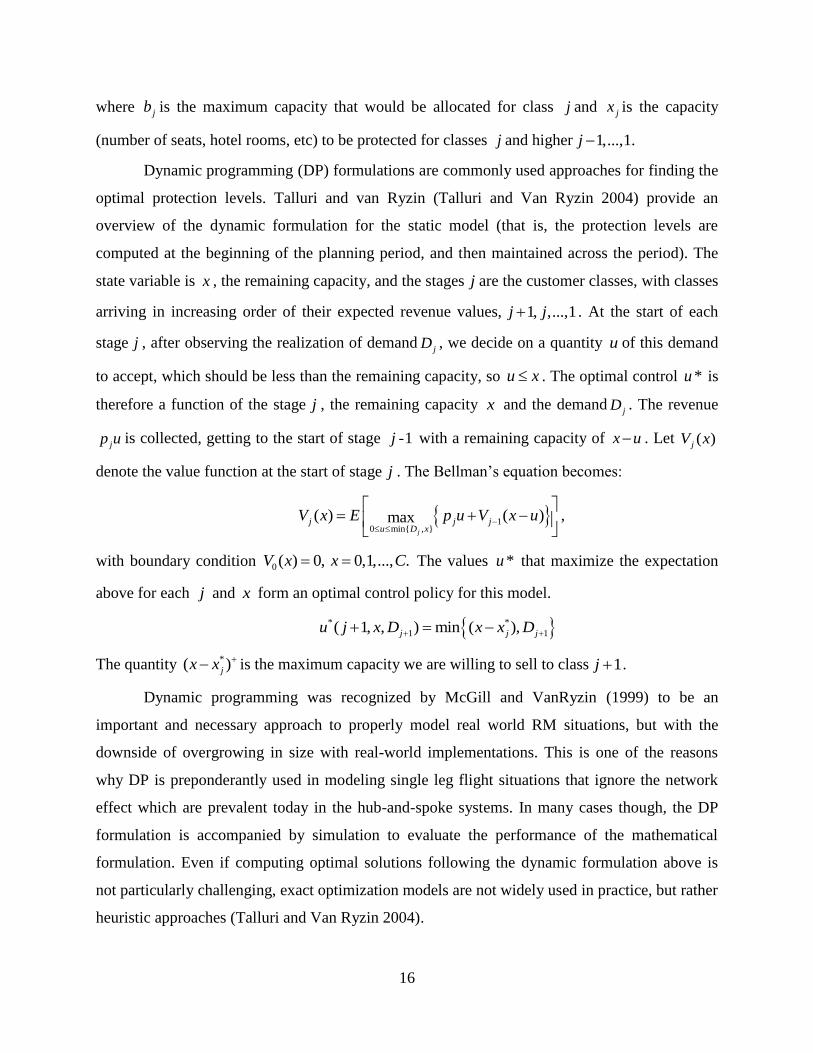
16
where jb is the maximum capacity that would be allocated for class j and jx is the capacity
(number of seats, hotel rooms, etc) to be protected for classes j and higher 1,...,1.j
Dynamic programming (DP) formulations are commonly used approaches for finding the
optimal protection levels. Talluri and van Ryzin (Talluri and Van Ryzin 2004) provide an
overview of the dynamic formulation for the static model (that is, the protection levels are
computed at the beginning of the planning period, and then maintained across the period). The
state variable is x , the remaining capacity, and the stages j are the customer classes, with classes
arriving in increasing order of their expected revenue values, 1, ,...,1j j . At the start of each
stage j , after observing the realization of demandjD , we decide on a quantity u of this demand
to accept, which should be less than the remaining capacity, so u x . The optimal control *u is
therefore a function of the stage j , the remaining capacity x and the demandjD . The revenue
jp u is collected, getting to the start of stage -1 j with a remaining capacity of x u . Let ( )jV x
denote the value function at the start of stage j . The Bellman‟s equation becomes:
10 min{ , }
( ) ( )maxj
j j ju D x
V x E p u V x u
,
with boundary condition 0( ) 0, 0,1,..., .V x x C The values *u that maximize the expectation
above for each j and x form an optimal control policy for this model.
* *
1 1( 1, , ) min ( ),j j ju j x D x x D
The quantity *( )jx x is the maximum capacity we are willing to sell to class 1j .
Dynamic programming was recognized by McGill and VanRyzin (1999) to be an
important and necessary approach to properly model real world RM situations, but with the
downside of overgrowing in size with real-world implementations. This is one of the reasons
why DP is preponderantly used in modeling single leg flight situations that ignore the network
effect which are prevalent today in the hub-and-spoke systems. In many cases though, the DP
formulation is accompanied by simulation to evaluate the performance of the mathematical
formulation. Even if computing optimal solutions following the dynamic formulation above is
not particularly challenging, exact optimization models are not widely used in practice, but rather
heuristic approaches (Talluri and Van Ryzin 2004).
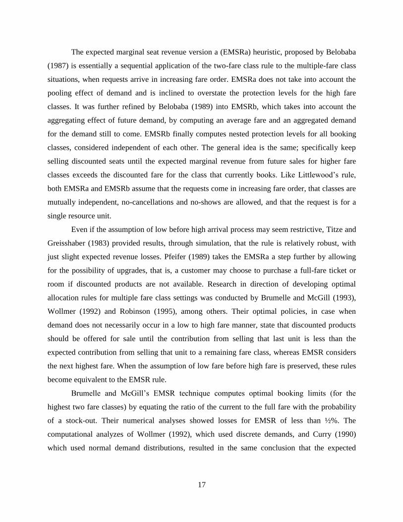
17
The expected marginal seat revenue version a (EMSRa) heuristic, proposed by Belobaba
(1987) is essentially a sequential application of the two-fare class rule to the multiple-fare class
situations, when requests arrive in increasing fare order. EMSRa does not take into account the
pooling effect of demand and is inclined to overstate the protection levels for the high fare
classes. It was further refined by Belobaba (1989) into EMSRb, which takes into account the
aggregating effect of future demand, by computing an average fare and an aggregated demand
for the demand still to come. EMSRb finally computes nested protection levels for all booking
classes, considered independent of each other. The general idea is the same; specifically keep
selling discounted seats until the expected marginal revenue from future sales for higher fare
classes exceeds the discounted fare for the class that currently books. Like Littlewood‟s rule,
both EMSRa and EMSRb assume that the requests come in increasing fare order, that classes are
mutually independent, no-cancellations and no-shows are allowed, and that the request is for a
single resource unit.
Even if the assumption of low before high arrival process may seem restrictive, Titze and
Greisshaber (1983) provided results, through simulation, that the rule is relatively robust, with
just slight expected revenue losses. Pfeifer (1989) takes the EMSRa a step further by allowing
for the possibility of upgrades, that is, a customer may choose to purchase a full-fare ticket or
room if discounted products are not available. Research in direction of developing optimal
allocation rules for multiple fare class settings was conducted by Brumelle and McGill (1993),
Wollmer (1992) and Robinson (1995), among others. Their optimal policies, in case when
demand does not necessarily occur in a low to high fare manner, state that discounted products
should be offered for sale until the contribution from selling that last unit is less than the
expected contribution from selling that unit to a remaining fare class, whereas EMSR considers
the next highest fare. When the assumption of low fare before high fare is preserved, these rules
become equivalent to the EMSR rule.
Brumelle and McGill‟s EMSR technique computes optimal booking limits (for the
highest two fare classes) by equating the ratio of the current to the full fare with the probability
of a stock-out. Their numerical analyses showed losses for EMSR of less than ½%. The
computational analyzes of Wollmer (1992), which used discrete demands, and Curry (1990)
which used normal demand distributions, resulted in the same conclusion that the expected

18
revenue from using the proposed heuristics are less than half of a percentage when compared to
the optimal revenue obtained through numerical integration.
All these three above mentioned rules (Littlewood‟s rule, EMSRa and EMSRb) and their
extensions can be used in a static fashion (once, at the beginning of the booking period), or in an
advanced static, or dynamic manner, where the demand distribution for each class is updated
periodically during the booking period to better reflect possible changes in demand patterns. This
allows the capacity allocation decisions to change based on the updated demand, permitting, for
example, for classes that were closed to become open in cases where the demand has not
occurred as expected.
As mentioned above, dynamic programming has been used in an effort to relax some of
the assumptions incorporated into the policies reflected by Littlewood‟s rule, EMSR and the
optimal policies discussed above. Gerchak et al. (1985) used DP in a bagel-shop environment,
determining if the shop should sell the bagels by themselves (low contribution) or sell them as
higher contribution items (sandwiches, for example). They treated the booking as a stochastic
Poisson process and relaxed the assumption of no batch bookings. Contribution to the model
were later brought by Lee and Hersh (1993) who extended the model to multiple fare situations
and Subramanian et al. (1999) who included overbooking, cancellations and no-show.
When discussing about RM, order fulfillment and customer satisfaction, we also have to
bring into discussion different predispositions and preferences that customers may have when it
comes to waiting for a service to begin or for a product to be delivered. Realizing that customers
have different sensitivities towards waiting, and not only to the price paid, is an important step
towards improving the RM related models. Kapuscinski and Tayur (2007) provide models that
incorporate this variable adversity towards waiting when the company quotes a due-date for its
two customer classes. The authors propose a heuristic and an optimal policy to the lead time
quotation problem in a make-to-order environment with stochastic demand, two customer
classes, deterministic processing times, and no cost for an early delivery date. Their paper also
incorporates an overview of the literature for the due-dates quotation research problem.

19
2.1.3 Overbooking
For a summary of relevant research regarding overbooking we refer to McGill and VanRyzin‟s
work (1999) to get a glimpse of the breakthroughs in this stream of research until the late „90s.
Overbooking rose naturally from the need of airlines to account for possible cancellations and
no-shows. Overbooking could lead to situations where customers are denied boarding or are
being moved to an inferior (but sometimes superior) class, having most of the times negative
effects on customers‟ satisfaction and decrease in perceived service quality. Even though it can
have both positive and negative impacts on revenues (Yoshinori 2002) and its negative side
effects cannot be completely eliminated, overbooking is becoming a necessity. A smart
overbooking system would control and balance the overbooking cost due to the probability of
customers being denied boarding (or lodging) with the lost revenue from flying with empty seats
(or having unoccupied rooms at the end of the day). Overbooking received a great deal of
attention from practitioners and academia and it has been researched for longer time than any
other RM related problem (McGill and van Ryzin 1999).
The initial overbooking work was on static, one period models (Beckmann and
Bobkowski 1958; Thompson 1961). Rothstein provided the first dynamic programming
formulation for the overbooking problem in his PhD thesis and future work (1968) and (1971) in
the airline industry and hotel overbooking. Overbooking situations in hotel industry were
initially analyzed by Ladany (1976), (1977) and Ladany and Arbel (1991) who extended
Rothstein‟s DP model to two customer classes.
The overbooking dynamic formulation for the static model with multiple classes is
succinctly presented in Talluri and van Ryzin (2004). The state variable is represented by the
number of reservations on hand, y, rather than the remaining capacity, x. With ( )jV y being
interpreted as the expected net benefit of operating the system from stage j onward, the Bellman
equation for the static model to account for cancellations and no-shows is as follows:
10 min{ , }
( ) ( )maxj
j j ju D x
V x E p u V x u

20
with boundary conditions (0) 0jV and 0
1
( ) , 0,y
i
i
V y E c Z y
for all classes and states
j , and with iZ either 1 or 0 depending if the customer shows up or not.
The more recent literature on overbooking is overwhelming in the number of issues and
assumptions taken into account in the developed models and proposed optimal or heuristic
solutions (Chatwin 1993; Chatwin 1999; Chatwin 1999; Karaesmen and Van Ryzin 2004), just to
mention a few.
2.2 HEALTHCARE
After about three decades of RM research, while the practice was successfully implemented in
airlines, hotels and rentals industries, as most representative, there is still at least one very
important industry where RM practices are being adopted slowly, or reluctantly: health care
industry, and more specifically, surgical units within hospitals. It can be argued that hospitals are
non-profit organizations, and not necessarily revenue maximizing units. This is not necessarily
true. Hospitals continue to survive and provide quality, indispensable services, only if they
recover and profitably reinvest the revenue generated by the wide range of services they provide
to a wide range of patients. As waiting times for elective surgeries are known to be increasing
and waiting queues are piling up, solutions are sought to decrease the waiting times while
maintaining an acceptable quality service (Strum, Vargas et al. 2008).
Surgical units within a hospital usually account for at least 60% of the total revenue
generated by that hospital. The truth is that people will continue to need surgeries and it is also
true that a good management of scheduling surgeries can lead to increased revenue for the
hospital, which cannot be seen at all detrimental, in the long run, to either the health of the
patient or of that of the institution. Additional revenue generated by a good surgery scheduling
policy can be reinvested so that the capacity will increase in the long run, and more patients
could be offered service and/or decrease waiting times. The conclusion that can be drawn is that
there is the need for a paradigm shift from the operating room (OR) as a cost center to that of a
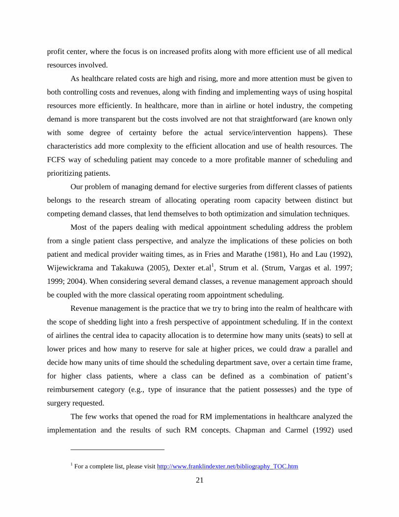
21
profit center, where the focus is on increased profits along with more efficient use of all medical
resources involved.
As healthcare related costs are high and rising, more and more attention must be given to
both controlling costs and revenues, along with finding and implementing ways of using hospital
resources more efficiently. In healthcare, more than in airline or hotel industry, the competing
demand is more transparent but the costs involved are not that straightforward (are known only
with some degree of certainty before the actual service/intervention happens). These
characteristics add more complexity to the efficient allocation and use of health resources. The
FCFS way of scheduling patient may concede to a more profitable manner of scheduling and
prioritizing patients.
Our problem of managing demand for elective surgeries from different classes of patients
belongs to the research stream of allocating operating room capacity between distinct but
competing demand classes, that lend themselves to both optimization and simulation techniques.
Most of the papers dealing with medical appointment scheduling address the problem
from a single patient class perspective, and analyze the implications of these policies on both
patient and medical provider waiting times, as in Fries and Marathe (1981), Ho and Lau (1992),
Wijewickrama and Takakuwa (2005), Dexter et.al1, Strum et al. (Strum, Vargas et al. 1997;
1999; 2004). When considering several demand classes, a revenue management approach should
be coupled with the more classical operating room appointment scheduling.
Revenue management is the practice that we try to bring into the realm of healthcare with
the scope of shedding light into a fresh perspective of appointment scheduling. If in the context
of airlines the central idea to capacity allocation is to determine how many units (seats) to sell at
lower prices and how many to reserve for sale at higher prices, we could draw a parallel and
decide how many units of time should the scheduling department save, over a certain time frame,
for higher class patients, where a class can be defined as a combination of patient‟s
reimbursement category (e.g., type of insurance that the patient possesses) and the type of
surgery requested.
The few works that opened the road for RM implementations in healthcare analyzed the
implementation and the results of such RM concepts. Chapman and Carmel (1992) used
1 For a complete list, please visit http://www.franklindexter.net/bibliography_TOC.htm

22
threshold curves to determine whether and when to apply discounts in order to increase the
capacity utilization and revenue yield within Duke‟s university diet and fitness center. Gerchak
et al. (1996) develop an advanced reservation planning policy for elective surgery patients when
the operating room capacity is common for both elective and emergency surgeries. In 2004,
PROS Revenue Management team along with Born et al. (2004) worked on optimizing the
performance of contracts with insurers at Texas Children‟s Hospital.
In a more recent article, Green et al. (2006) analyze the patient scheduling problem faced
by an MRI diagnostic facility and they identify threshold policies to manage patient demand and
the capacity allocation (appointment scheduling and dynamic priority) by using a finite-horizon
dynamic program. The policy determines at each point, based on a switching index, which
patient class should be serviced next: inpatients, outpatients or emergencies. While their
assumption is that examination times are fixed and equal to the allotted time slots, we
incorporate in our analysis the service time stochasticity from the beginning.
Recently, Olivares et al. (2008) analyzed the situation of OR time allocation to a single
surgical procedure with random service time. Their paper provides a general structural model to
estimate the overage and underage costs in a newsvendor setting, with an application in reserving
OR time. Specifically, the decision on OR time allocation to a specific surgical case (emergency
or elective) is analyzed from the perspective of the factors that influence demand, while
providing insight into what the cost parameters are for the hospital under study. Based on past
history of observed time allocation and actual case durations, the authors show that the hospital
places too much or too little value on idle time and overtime, with more accurate results when
duration forecasting bias is incorporated in the model. The structural modeling approach
employed when tackling the problem of reserving OR time to surgical cases provides a general
framework that hospitals, as well as other newsvendor like settings, could use when deciding
how much time to reserve for individual service (surgical) cases. From past observations one can
derive the overage/underage cost ratio which becomes the input for the decision of how much
OR time to reserve for a particular surgical case.
Lan, Gao et al. (2008) propose several models for determining online booking limits
under static and dynamic policies, where only limited information about the demand is required,
specifically upper and lower bounds for the various demand classes. The constant demand is
generated by arrivals from multiple fares/classes that request a single unit of a discrete resource

23
(rooms, seats, etc). The analysis, carried from perspective of competitive ratio and absolute
regret performance criteria, derives online and off-line nested booking limits that are shown to
perform, on average, similar to the more widely used EMSR and EMSRb. While the use of only
limited demand information is attractive in practice, the authors point out the fact that the
booking limits are sensitive to departures of the specified demand parameters from the true ones.
Gupta and Wang (2008) propose several heuristics to help clinics decide how to ration
the available slots between walk-ins (same-day appointments) and regular patients (advance
booking) who may have a preference for both the slot time and their primary care physician
(PCP). Same-day demand and caller‟s characteristics are needed to decide on an accept/reject
decision for a caller for a specific slot, as well as for the physicians‟ booking. While their
numerical results show that the proposed heuristics on booking limits are close to optimal, they
don‟t assume variability in the service provided (i.e., it is assumed that each patient‟s visit will
not go beyond the allotted slot time). The patient generated revenues, function of the type of
booking (regular or same-day patients) and its PCP preference, are diminished by the costs of
insufficient capacity, unused slots or denied requests. The booking-limit policy in the presence of
one doctor, for example, suggests the optimal number of slots to be reserved for same-day
patients, * 1( )b k F
, where 1F is the inverse c.d.f. for same day demand, is a cost
ratio, and k is the clinic‟s daily slot capacity. When two or more doctors are available, the
threshold booking limits dictate when to close the bookings (deny access) for a customer,
function of his/her preferences for doctor and/or time slot. The analysis is from the perspective of
a clinic that offers same length appointment slots, and where the average contribution per slot is
the same for all regular patients who get an appointment with their PCP of choice. In our
analysis, we explicitly consider the service time variability, and thus, when coupled with revenue
per class of service, makes sense to deny (or postpone) a request to save a slot for future patients.
The awareness of unacceptable long waiting times for elective surgeries within the public
hospital system became more noticeable in the past decade, thus dealing with this issue should be
a focus not only at the hospital, but at the national/governmental level as well. An increase in
admission rates to the hospital should be coupled with an increase of the available hospital
resources (doctors, nurses, beds, etc). One source of funding this capacity increase can be the
internal financial resources (re-investing the profits), and the follow-up conclusion is that
hospitals, and surgical units in particular, need to have a shift of paradigm, and change their
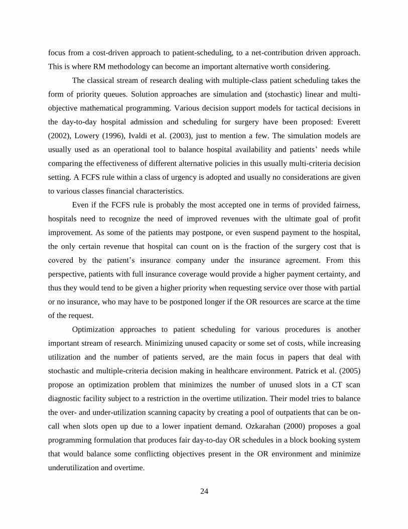
24
focus from a cost-driven approach to patient-scheduling, to a net-contribution driven approach.
This is where RM methodology can become an important alternative worth considering.
The classical stream of research dealing with multiple-class patient scheduling takes the
form of priority queues. Solution approaches are simulation and (stochastic) linear and multi-
objective mathematical programming. Various decision support models for tactical decisions in
the day-to-day hospital admission and scheduling for surgery have been proposed: Everett
(2002), Lowery (1996), Ivaldi et al. (2003), just to mention a few. The simulation models are
usually used as an operational tool to balance hospital availability and patients‟ needs while
comparing the effectiveness of different alternative policies in this usually multi-criteria decision
setting. A FCFS rule within a class of urgency is adopted and usually no considerations are given
to various classes financial characteristics.
Even if the FCFS rule is probably the most accepted one in terms of provided fairness,
hospitals need to recognize the need of improved revenues with the ultimate goal of profit
improvement. As some of the patients may postpone, or even suspend payment to the hospital,
the only certain revenue that hospital can count on is the fraction of the surgery cost that is
covered by the patient‟s insurance company under the insurance agreement. From this
perspective, patients with full insurance coverage would provide a higher payment certainty, and
thus they would tend to be given a higher priority when requesting service over those with partial
or no insurance, who may have to be postponed longer if the OR resources are scarce at the time
of the request.
Optimization approaches to patient scheduling for various procedures is another
important stream of research. Minimizing unused capacity or some set of costs, while increasing
utilization and the number of patients served, are the main focus in papers that deal with
stochastic and multiple-criteria decision making in healthcare environment. Patrick et al. (2005)
propose an optimization problem that minimizes the number of unused slots in a CT scan
diagnostic facility subject to a restriction in the overtime utilization. Their model tries to balance
the over- and under-utilization scanning capacity by creating a pool of outpatients that can be on-
call when slots open up due to a lower inpatient demand. Ozkarahan (2000) proposes a goal
programming formulation that produces fair day-to-day OR schedules in a block booking system
that would balance some conflicting objectives present in the OR environment and minimize
underutilization and overtime.

25
The scheduling literature in manufacturing also considers rolling-horizon models with the
objective of identifying a job/service sequence that minimizes either expected or total cost
(Pinedo 2001). Some of the underlying assumptions though are that all the jobs will be processed
by the end of the planning period and that the jobs are either released at the beginning or at some
(random) points during the horizon. It is known that even for the assumptions of deterministic
processing times and weights, the situations involving job release dates are NP-hard problems
(Lenstra, Rinnooy et al. 1977). Recently, Chou et al. (2006) analyzed the problem of minimizing
the expected total weighted completion time of a set of jobs with release dates and stochastic
processing times and analyzed the performance and proved the asymptotic optimality of their
proposed WSEPTA (weighted shortest expected processing time among available jobs) heuristic.
While our problem deals with the broader aspect of resource allocation and accept/postpone
decisions to maximize expected revenue, some similarities exist, especially the release dates,
stochastic processing time and job weights/priorities. But when dealing with patients‟ request for
service, once the clinic and the patient decide on an appointment date, it is not re-evaluated and
changed every time a new unit of demand occurs, as is the case in Chou et al.‟s WSEPTA.
The main conclusion that we draw from inspecting the work done in the areas of revenue
management and scheduling is that there is not a lot of literature that covers resource allocation
to classes of demand that use up a variable amount of that resource. We try to make our
contribution in filling this gap by addressing the allocation of a continuous resource across
several competing customer classes that necessitate a variable usage of that resource. The
operating room scheduling arena is one where the stochastic nature of the procedures‟ times has
a large effect on the performance and bottom-line profit of the clinic. The average contribution
per unit of resource is a function of both the procedure type and the patient‟s insurance category.
The final goal in finding an optimal resource allocation between these competing customer
classes is to increase the expected revenue for the surgical department. This goal is not a trivial
one to attain, especially when the resource usage per request is variable, is relatively limited per
scheduling period and customers have different sensitivity towards waiting. This work tries to
bridge the gap between OR time allocation and patient segmentation through the use of an
optimization model and the implementation of some modified techniques pertaining to the area
of RM.

26
2.3 MAPPING REVENUE MANAGEMENT CONCEPTS TO THE HEALTHCARE
ENVIRONMENT
The yield-management practices apply to all service operations that meet certain well-defined
criteria. We map the main characteristics of a yield management system to the health care
environment to assess how the specific characteristics within a hospital‟s surgical department
need to be interpreted in the context of yield management.
Classical RM practices apply to systems where identical or undifferentiated products
satisfy various types of customers (the same room in a hotel can be sold to a low-fare class
customer or to a business-traveler, at a higher price; or, the same seat on a flight can be sold at
various prices depending on when it is booked, etc). When the product units offered are all alike,
then we know exactly the initial inventory on hand and we can say that this capacity is relatively
fixed in the short run, because it is almost impossible to add an extra seat on an airplane or a
room in a hotel. In the surgical context, due to the customized nature of the service rendered, and
to the somehow large variation in their durations from patient to patient, even for the same type
of surgery, it is not that straightforward to set a priori the capacity of an OR when expressed in
terms of number of surgeries. This is why we need to express the capacity of the service/surgical
facility in time units (minutes, hours, or multiples).
Health services can be in some way different from typical revenue-management users
(hotels, airline, car rental companies) in that, among other things, treatments for health issues are
individually prescribed. In particular, within a hospital‟s surgical unit, there are many types of
surgeries that are being performed, and even for the same type of surgery, the duration may vary
quite a lot from patient to patient (and sometimes, from doctor to doctor), due to the gravity of
the illness or possible complications that could arise, unexpectedly, during the surgery (Strum,
Sampson et al. 2000). This leads to difficulty in accurately assessing a priori the capacity of an
OR that is opened 8 hours a day, when the definition of the product of service is the surgery
performed. This may be the natural way of interpreting the type of product provided by the
surgical department, but this definition can create difficulties when revenue management
techniques are being applied. This leads us to define the surgical product as a time unit, the same
unit used to express capacity. Now, the expected duration of a surgery can be expressed in terms

27
of the time units and the hospital can have a more accurate estimation of the upper capacity of a
surgical suite (determined by the duration of the regular time plus some possible overtime).
When patients arrive to request surgery of a certain specialty (or, in most cases, when the
physician requests a surgery for the patient), he/she is allocated units of time that are estimated to
cover the expected duration of that sort of procedure. By converting all arriving demand over a
predefined horizon (requests for elective surgeries) in time units, we will be able to determine the
demand (in time units) and to further allocate capacity (time units) to various classes of
customers (patients).
The demand for service/surgical time arrives from patients that are requesting elective
surgeries. We model the booking limits for the accept/postpone decision when a request arrives
to the system, and try to find an efficient policy that will lead to increased expected revenue
generated by the performed procedures. We do not model the additional stay of patients in the
hospital as part of their recovery time, but we do recognize that a systemic approach is necessary
for improving hospital‟s overall performance.
The hospital/clinic is assumed to be able to differentiate among patients, who can be
segmented into clearly-identified classes (groups or categories) based on some contractual
agreement set a priori - their reimbursement (i.e., type of insurance they possess with full
coverage, partial coverage, or no insurance at all), but also based on the type of surgery they
request. If we think about making a parallel between an airline company and a hospital, then a
passenger who requests a seat of a certain fare on a flight leg between two specific cities is the
same as a patient having some type of insurance, who requests an elective surgery (e.g., hip
replacement, plastic surgery, etc.).
The hospital, like the airline company, needs to estimate the demand for that type of
surgery (the demand for that flight-leg) and assess the distribution of the insurance types within
those requests for that type of surgery (requests for various fare-classes). In both cases, future
allocation of capacity to demand is made under the uncertainty assumption about the future
demand, with the specification that in some service cases (like the hospital), customer are more
willing (and understanding about it) to wait for service to be rendered than in the airline case. At
the same time, a hospital can have several operating rooms which may have various
requirements as to which types of procedures they could handle. When coupled with service time
variability, it is not that obvious for a surgical ward how to optimally decide on the time to

28
allocate for each type of surgery and where to place those surgeries. Having multiple ORs is, in a
sense, similar to having multiple flights between same two cities. While for airlines the units of
demand and capacity are discrete, we assume the allocation of a continuous resource (time).
Hospitals have large databases of records of past data and can retrieve the information
about patients‟ insurance types and surgeries requested in order to determine potential average
revenue per procedure, as well as estimations for procedures‟ duration distributions. It was
shown by Strum et.al. (2000) that the lognormal (with 2 and 3 parameters) and normal
distributions are good estimates for procedure durations, with the lognormal appearing to be
superior to the normal (empirically validated through testing on larger samples).
A more difficult task, though, is the one of predicting the future demand for various types
of surgeries, since we cannot easily talk about a seasonality effect or “peak” periods like in
airline or hotel management. There are many factors that limit an accurate prediction of demand
in healthcare, which are related to both limited information gathered on past demand and to the
inability to fully account for all major factors that affect demand in the long run. In most cases,
the demand recorded is, in fact, censored demand, because health-care providers do not routinely
track patients who are unable to book an appointment due to the limited service capacity relative
to the demand over the open booking period (Gupta and Wang 2008). Thus, a fraction of
requests passes by unrecorded, or, at best, is recorded only when there is a match with available
capacity. This leads to a distortion and lag in the lead time of demand. Aggregated over time,
these requests that are registered only when available capacity can accommodate them, and not
at the exact moment when they occurred, lead to a distortion in true demand, which propagates
into the demand forecasting models. This distortion is further deepened by the always changing
mix of requests for service, which are further influenced by many other demographic factors.
One of the more recent research and practice streams in healthcare, known as advanced
access (Murray and Berwick 2003; Gupta, Potthoff et al. 2006) is focusing on outpatient
scheduling through better managing clinic capacity to accommodate more same-day appointment
requests. While our research is looking for managing capacity in scheduling elective surgeries,
where same-day appointments are almost impossible, the main goal is also to provide timely
access to healthcare in a manner that would be beneficial for the patients‟ well-being as well as
for the healthcare unit‟s financial soundness.

29
Surgical units within a hospital bring approximately 60% of the hospital‟s revenue; they
are indeed the profit centers of the hospital and they need to think in terms of maximizing the
revenue, which will result in contribution improvements. If more revenue is brought by the
surgical units, this means that the unit can survive and sustain itself, being able to offer more
service in the future. Surgical units need to look at surgery scheduling from a revenue
maximization perspective. The optimization model we propose is a neutral one, which should not
create incentives for unethical practices (scheduling more surgeries than necessary or indefinitely
postponing lower category patients). Additional restrictions can be imposed in the model
formulation (or in practice) that can take care of some ethical questions that could arise.
Patients who opt for elective surgeries usually request service some time ahead of the
actual surgery date. After the request is received, the scheduling department needs to make a
decision/commitment of when to schedule this patient at a time when future demand is uncertain.
As in the airline or hotel services, bookings are made some time in advance. The difference here
is that in the airline or hotel industry, when a customer books a seat or a room, he/she specifies
exactly when he/she needs the service (there is still a chance that the flight or hotel could be
already booked for that specific date, requiring the passenger to reconsider either booking for
another flight or fare-class). Still, the passenger/traveler will know at the booking time if he can
get the seat/room requested. In the healthcare context, when patients (or their physicians) call to
schedule a surgery date, he/she does not have full control over when the surgery is going to be
performed. The decision is taken by the scheduling department after reviewing and taking into
account various criteria, among which doctors‟ availability and preferences, ORs, nurses, and, as
we are proposing here, patient‟s reimbursement category (i.e., insurance type). The patient may
get an immediate answer as to when the surgery will be performed at a later point in time or they
may wait for a few days to lock-in a surgery date.
Our intention in this work and its future extensions is to model the problem so that the
hospital can make more informed decisions when quoting a surgery date at the moment of the
request (more like an instant due-date quoting in the make-to-order environment), and focus on a
dynamic booking system that constantly updates based on both already materialized and
potential future demand. Quoting a reliable and acceptable appointment date is similar to quoting
reliable due-date in a manufacturing setting. In a make-to-order (MTO) industry setting a reliable
due date quotation is very important for the manufacturing company. For example, Kapuscinski

30
and Tayur (2007) propose a heuristic for the lead time quotation problem in a MTO environment
with stochastic demand and deterministic processing times, while accounting for future arrivals.
What distinguishes our work from theirs is that our model is not restricted to two demand classes
of customers and deterministic service time We deal with stochastic service times, and, even if
we do not include explicitly a cost for an early delivery date, once the due date (appointment
time) is quoted, it is assumed that the customer would expect the service to be done at that date
and he/she may not accept an earlier date if one becomes available later.
Customers often require, at the time they make a request for service, a confirmation of
when their service (surgical procedure) would be performed. Different patient classes have
different sensitivities to the waiting period (not necessarily based on the urgency of the
procedure), and it may happen that a customer who is quoted a service time further into the
future will decide not to wait for the service and seek it somewhere else, thus depriving the
hospital of some potential revenue. Thus, service postponement may come at a cost for both the
hospital and the patients. Because patients compete for the same OR capacity, the service
provider should take this time sensitivity into account when deciding how much OR time to
reserve for various classes of patients and surgeries. This is one of the reasons why a RM like
approach in a healthcare setting would reduce the risk of losing potential revenue in the long run.
In the context of surgical units, we focus on allocating a single resource – time units –
among various types of surgery and patient reimbursement categories. We can think of these
reimbursement categories as the various insurance types (private or governmental, full, partial, or
even no coverage) that a patient elected to have over a certain time frame. We can group the
types of insurance coverage into three broad defined categories: full, partial, and none/minimal.
The scheduling period can be a day, a week, or the planning period that the surgical unit is using
when allocating time for various procedures or across doctors and subspecialties.
Unlike some of the business environments (hospitality, airline, rental) where the
customer is lost if he/she cannot be served at the time when demand occurs, in most of the
healthcare related situations the customers (in- and out-patients) can be delayed, but at a cost. In
our case, since we deal with elective surgeries, the patients can be postponed until a later date,
considering time availability for their class and a class-related sensitivity to wait. Based on
expected demand from each class of elective patients and on the expected revenue per time unit
that each class generates, we compute protection levels, defined as the number of surgical time

31
units to be protected for each customer class. The optimization model finds those protection
levels that maximize the expected revenue obtained by the healthcare unit. We also propose a
heuristic for protection levels computation, which also generates, due to the variability in
resource usage per surgery, distribution of protection levels; we show how they can be used to
decide on time protection/allocation for each patient reimbursement category within each surgery
type function of the overtime to regular time costs ratio.
In healthcare, it may also happen that patients cancel their appointments in the last
minute or fail to show up altogether, without previous notice, and even if they do show up, it
may be that they are late. All these, coupled with emergency patients (impromptu arrivals) lead
to the implementation of overbooking practices, considered necessary evils that need to be put in
practice to hedge against lost demand and for better management of the patient flow. Even if
postponing patients for a later time that day or rescheduling them for another day is not desired,
these options are used in practice (Moore, Strum et al. 2008) and should be taken into account
when booking patients‟ appointments and deciding on an appointment schedule for that period.
Patients‟ arrivals patterns should be observed and forecasted, and, if overbooking is a viable
option, it should be addressed appropriately. Maybe offering the postponed patient a monetary
compensation, like airlines do with their bumped passengers, could alleviate how patients regard
the whole postponing practice/necessity.
Many hospital departments (like the surgical departments) usually provide services to
several broad groups of patients. First, we have the inpatients, whose demands vary during the
day, and for whom the surgery should be performed before the patient can be released; then there
are the emergency and urgent patients who must be served as soon as possible, having the
highest priority. The outpatients constitute the third group that is served by hospitals; they
request service in advance, at their doctor‟s request, and they should show up at the appointment
date set by the scheduling personnel. Elective surgeries could be either inpatient or outpatient
procedures, and our research is looking to manage the demand for elective surgeries by finding
an efficient implementation of RM techniques in designing an appointment schedule that will
maximize expected revenue along with keeping the operational costs under control.
With hospitals‟ costs and insurance premiums on the rise, and with managers under
constant pressure to manage these facilities in a more efficient and effective way in order to

32
reduce costs while increasing revenues and the quality of service, there should be a change of
paradigm in that hospitals should be regarded as profits centers and managed as such.
Currently in US about 16% of the population is uninsured, with the rest of the population
having various types and degrees of insurance. Most Americans have health insurance through
their employers. But employment is no longer a guarantee of health insurance coverage2.
Broadly, we can divide the whole pool of patients that request service at a certain hospital based
on their financial characteristics (which could be rather different) in patients with full coverage,
partial coverage and minimum/no coverage at all. All of them are entitled to service and their
business could be lost if the service is postponed longer than the patients‟ expected willingness
and availability to wait for service. With medical tourism as a rapidly growing practice, more
and more people look to traveling to another country to obtain health care, especially elective
procedures, for which there are several months long waiting lines in US or Canada.
Much of the RM literature in the airline and hotel industry assumes that a customer is lost
if his/her demand cannot be met at the requested time. In healthcare, a patient‟s request for
surgery can usually be postponed/delayed for some time with the price of incurring appropriate
penalties (either in forms of penalty costs or deferred revenue). Another difference worth
mentioning is that in the classic RM setting, the customers are the ones that dictate the time of
service rendered, in the sense that they request a flight for a particular date and time, a room for a
particular night(s), etc; on the other hand, in the healthcare setting, patients usually have little, or
no decision on when the intervention/surgery would take place. Other factors (degree of
emergency, doctor, nurse and room availability, among others) are factors that influence the time
when the service will be provided. Patients usually consider this postponement of service as an
acceptable situation (or necessary evil) as long as it does not go beyond some subjective
estimation of their willingness to wait.
2 See, for example, http://www.nchc.org/facts/coverage.shtml
33
3.0 MODELING THE PROBLEM OF CAPACITY ALLOCATION UNDER
VARIABLE SERVICE TIME ASSUMPTION
This third chapter is dedicated to problem treatment for the single resource allocation among
competing customer classes segmented based on the type of service requested and their
contribution category. The results translate in protection levels for these customer classes, which
are computed in a nested fashion, but are partitioned in nature. We start by presenting the
situation when the resource utilization per accepted request is deterministic, and then show how
the setting of protection levels change under the consideration that accepted requests for service
consumes a variable resource amount.
Firstly, we present the protection levels computation under the traditional, i.e.
deterministic time consideration, with respect to two assumptions on the magnitude of demand
from the two groups with respect to available capacity. Secondly, we show how these protection
levels are changing when we deal with a random resource usage per accepted request. This
situation is encountered in practice, both in services and manufacturing, where is a relatively
high degree of service/product customization. Thirdly, we are going to extend the results
obtained for the two-class case to the three-class and n-class cases to better reflect the more
realistic situations that arise in practice.

34
3.1 DETERMINISTIC CASE
Assume that a system has total capacity of C and that there are two groups of customers, with
each customer requesting exactly one unit of total capacity. Each customer from group 1 pays 1p
and each customer from group 2 pays 2p , with
1 2p p . Let if be the probability density
function for group i‟s demand,iD its realized value, and
iF its cumulative distribution. For
simplicity, assume that theif ‟s are continuous. group 2 customers arrive before group 1
customers, there are no cancellations, and overbooking is not permitted. Let x denote the
protection level, that is, the number of units of capacity reserved for group 1 customers.
We consider two cases:
Case 1. Neither group 1 nor group 2 demand would exhaust the system capacity, but total
demand would, so that the capacity allocation problem is nontrivial. That is, 1[ ] 1P D C and
2[ ] 1P D C , but 1 2[ ] 1P D D C .
Case 2. The demand 1D of group 1, the class that contributes more per unit of resource,
would not exhaust system capacity, but the demand 2D of group 2, the class that contributes less
per unit of resource, would exhaust system capacity, i.e., 1[ ] 1P D C and
2[ ] 1P D C .
In Case 1, the return for a protection level x is given by
2 2 1 1( ) min{ , ) min{ , }R x p D C x p D x .
The expected return is given by:
2 2 2 2 1 1 1 1
0 0
( ) ( ) ( ) ( ) ( ) ( )
C x x
C x x
ER x p yf y dy p C x f y dy p yf y dy p xf y dy
The value of x, x*, that maximizes ER(x) must satisfy the condition
21 2
1
[ *] [ *] 0p
P D x P D C xp
. (3.1)
The expected loss from group 1 brought about by setting the protection level at x* is
1 1[ *]p P D x and the expected loss from group 2 is 2 2[ *]p P D C x . Equation (3.1) thus
dictates that the protection level x* should be set so as to exactly balance the expected revenue
losses from the two groups of customers.

35
In Case 2, the situation considered by Littlewood (1972, republished 2005),
2[ *] 1P D C x , so that (3.1) reduces to
21
1
[ *] 0p
P D xp
(3.2)
and hence, we have
2
1
1
1* (1 )p
px F .
Littlewood‟s formula (3.2) is a fundamental result for revenue management, and is a
critical component of later, more general, methodologies such as Belobaba‟s (Belobaba, 1989).
3.2 RANDOM RESOURCE REQUIREMENTS
Now we consider a situation in which the amount of the scarce resource (space, time, etc.)
required by each customer is random. For example, one manages a flat-fee legal clinic that
serves both walk-in customers and those covered by employer-sponsored legal insurance.
Consultation times are random, but he has historical data that permit him to estimate the
distribution of time required to service a customer of either type. Professional ethics require him
to take customers on a first-come-first served basis and to complete a consultation no matter how
much time it requires. Customers covered by legal insurance pay less for a consultation than do
walk-ins. The question becomes how much of the fixed opening hours of the clinic should he
reserve for walk-in customers?
As before, assume that the system has total capacity of C and that there are two groups of
customers. Each customer from group i pays ip regardless of how much capacity he/she uses,
with 1 2p p . The density for the total number of units of capacity demanded by group i is
if .
Let ijT be a random variable representing the amount of resource used by a customer j of group i.
Assume that each value ijt , a realization of ijT , is small enough relative to C so that it is possible
to exactly schedule any desired level of service. Let1
iN
i ij
j
D t
, i =1,2 be the total demand from

36
group i, where iN is a random variable representing the number of customers of group i
requesting service.
Let /ij i ijQ p T be the contribution per unit of resource by a generic scheduled customer j of
group i. For convenience, let /i i iQ p T be a realization of ijQ for a scheduled customer in group
i. 1Q and
2Q are both random variables. Let [ ] , 1,2i iE Q i . It is also helpful to have notation
for the conditional expectations. Let 1 2| 1 2[ | ], 1,2i Q Q iE Q Q Q i and
1 2| 1 2[ | ], 1,2i Q Q iE Q Q Q i . Although 1 2p p , because
1Q and 2Q are random, it is not
certain that 1 2Q Q . Let θ denote the probability that
1Q is greater than 2Q , that is,
2 2 2 1 12 1
1 1 1 2 2
/[ ] 1
/
Q p T T pP Q Q P P
Q p T T p
Note that 1 2 1 2| |[ ] (1 )i i i Q Q i Q QE Q , i = 1,2, so that
1 2|i i Q Q as θ→1;
1 2|i i Q Q as θ→0; 1 2 1 22| 1|Q Q Q Q and
1 2 1 22| 1|Q Q Q Q .
With probability (1-θ), group 1 customers are less profitable, on a per-unit basis, than
group 2 customers. In that situation, allocating x resource units to group 1 is an allocation
decision, as opposed to a way to “protect” part of a scarce resource for the more financially
desirable customer group. In order to keep the terminology consistent, however, we continue to
refer to x as the protection level even when individual utilizations are random. The next result
shows that when utilizations are random, a unique protection level exists for Case 1, with the
prices of equation (3.1) replaced by the expected contributions per unit in (3.3).
Theorem 1: Under the conditions of Case 1, when customer resource utilization is
random, the unique optimal protection level for group 1, x*, satisfies the condition
21 2
1
[ *] [ *] 0P D x P D C x
. (3.3)
Proof: Let x denote the protection level for group 1. In Case 1, total demand from either
customer group alone is less than C, so the expected return with respect to the contribution per
unit of resource is given by
1 2 1 2
1 2 1 2
2| 2 1| 1 1 2
2| 2 1| 1 1 2
min{ , } min{ , } if ( )
min{ , } min{ , } if
Q Q Q Q
Q Q Q Q
D C x D x Q QR x
D C x D x Q Q
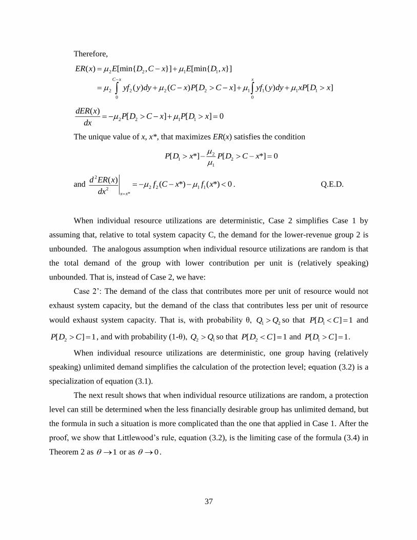
37
Therefore,
2 2 1 1
2 2 2 2 1 1 1 1
0 0
( ) [min{ , }] [min{ , }]
( ) ( ) [ ] ( ) [ ]
C x x
ER x E D C x E D x
yf y dy C x P D C x yf y dy xP D x
2 2 1 1
( )[ ] [ ] 0
dER xP D C x P D x
dx
The unique value of x, x*, that maximizes ER(x) satisfies the condition
21 2
1
[ *] [ *] 0P D x P D C x
and 2
2 2 1 12*
( )( *) ( *) 0
x x
d ER xf C x f x
dx
. Q.E.D.
When individual resource utilizations are deterministic, Case 2 simplifies Case 1 by
assuming that, relative to total system capacity C, the demand for the lower-revenue group 2 is
unbounded. The analogous assumption when individual resource utilizations are random is that
the total demand of the group with lower contribution per unit is (relatively speaking)
unbounded. That is, instead of Case 2, we have:
Case 2‟: The demand of the class that contributes more per unit of resource would not
exhaust system capacity, but the demand of the class that contributes less per unit of resource
would exhaust system capacity. That is, with probability θ, 1 2Q Q so that
1[ ] 1P D C and
2[ ] 1P D C , and with probability (1-θ), 2 1Q Q so that
2[ ] 1P D C and 1[ ] 1P D C .
When individual resource utilizations are deterministic, one group having (relatively
speaking) unlimited demand simplifies the calculation of the protection level; equation (3.2) is a
specialization of equation (3.1).
The next result shows that when individual resource utilizations are random, a protection
level can still be determined when the less financially desirable group has unlimited demand, but
the formula in such a situation is more complicated than the one that applied in Case 1. After the
proof, we show that Littlewood‟s rule, equation (3.2), is the limiting case of the formula (3.4) in
Theorem 2 as 1 or as 0 .

38
Theorem 2: Under the conditions of Case 2’, when customer resource utilization is
random, the unique optimal protection level for group 1, x*, satisfies the condition
1 2 1 2
* * * *
1 1 1| 1 2 2 2| 2[ ] 1 [ ] [ ] 1 [ ] 1
Q Q Q QP D x P D x P D C x P D C x
(3.4)
Proof: As before, let x denote the capacity allocated to group 1; C-x is allocated to group
2. The return is computed as follows:
(a) When 1 2Q Q , which occurs with probability θ, group 1 uses capacity
1min{ , }D x
and group 2 uses all the capacity allocated to it, C-x. The expected return with respect to the
contribution per unit of resource is thus
1 2 1 22| 1| 1( ) ( ) min{ , }Q Q Q QR x C x D x
(b) When 1 2Q Q , which occurs with probability (1-θ), group 1 uses all the capacity
allocated to it, x, and group 2 uses capacity 2min{ , }D C x . Thus, the return with respect to the
contribution per unit of resource is given by:
1 2 1 21| 2| 2( ) min{ , }Q Q Q QR x x D C x .
The total expected return is thus given by:
1 2 1 2 1 2 1 2
1 2 1 2 1 2
1 2 1 2 1 2
2| 1| 1 1| 2| 2
2| 1| 1 1| 1
0
1| 2| 2 2| 2
0
( )
[ ( ) min{ , }] (1 ) [ min{ , }]
( ) ( ) ( )
(1 ) ( ) ( ) ( )
Q Q Q Q Q Q Q Q
x
Q Q Q Q Q Q
x
C
Q Q Q Q Q Q
C x
ER x
E C x D x E x D C x
C x yf y dy x f y dy
x C x f y dy yf y dy
x
Differentiating with respect to x and equating the derivative to zero we have:
1 2 1 2 1 2 1 22| 1| 1| 1 2| 2
( )(1 ) [ ] (1 ) [ ] 0Q Q Q Q Q Q Q Q
dER xP D x P D C x
dx
The unique value of x, x*, that maximizes ER(x), satisfies the condition:
1 2 1 2
* * * *
1 1 1| 1 2 2 2| 2[ ] 1 [ ] [ ] 1 [ ]1 Q Q Q QP D x P D x P D C x P D C x
and 1 2 1 2
2
1| 1 2| 22*
( )( ) (1 ) ( ) 0Q Q Q Q
x x
d ER xf x f C x
dx
, which makes it a global
maximum. Q.E.D.

39
Corollary 3: Under the conditions of Case 2’, when customer resource utilization is
random, but it is known with certainty if 1 2Q Q or
1 2Q Q , the unique optimal protection level
for group 1, x*, satisfies the condition
21
1
[ *]P D x
if
1 2Q Q
and
12
2
[ *]P D C x
if
1 2Q Q .
Proof: As 1 in (4), we have 1 2 1 21| 1 2|[ *]Q Q Q QP D x , and because
1 2|i i Q Q as
1 , we have 21
1
[ *]P D x
, which is equation (3.2) when
1 2[ ] 1P Q Q . For 0 we
have 1 2 1 22| 2 1|[ *]Q Q Q QP D C x , and because
1 2|i i Q Q as 0 , we have
12
2
[ *]P D C x
. Q.E.D
3.3 EXTENSION TO MULTIPLE CLASSES
Assume that a system has total capacity of C and that there are n groups of customers. Each
group 1 customer pays 1p , each group 2 customer pays
2p , and each group n customer pays np ,
with 1 2 np p p . Each customer from group i requests a random number of units of
capacity, it . The demand density for Group i is
if , and its realized value is iD . For simplicity,
assume that theif ‟s are continuous. Customers arrive in a random order, there are no
cancellations, and overbooking is not permitted. Let ix denote the protection level, that is, the
number of units of capacity reserved for groups 1, 2 , …, i customers.
As before, let /i i iQ p T and let [ ] , 1,2,...,i iE Q i n . Let [ : ]ki k nQ Q and let
[1: ] [2: ] [ : ]n n n nQ Q Q represent an ordering of the variables iQ . There are n! possible

40
orderings. Let 1 21 2
| [ | ]i i i nn
i Q Q Q i i i iE Q Q Q Q , 1,2,...,i n and 1 2 ... ni i i denote the
probability of the ordering [1: ] [2: ] [ : ]n n n nQ Q Q , i.e.,
1 2 1... [ ]n ni i i i iP Q Q . Now we have
1 2 1 2
1 2
... |
...
[ ]n i i in
n
i i i i i i Q Q Q
i i i
E Q , i = 1,2,…,n so that 1 2
| i i ini i Q Q Q as
1 2 ... 1ni i i .
There are two distinct cases to consider:
Case 1: None of the groups‟ demand would exhaust the system capacity, but total
demand would, so that the capacity allocation problem is nontrivial, i.e., [ ] 1iP D C ,
1,2,...,i n , but1 2[ ] 1nP D D D C .
The revenue for protection levels 1 2 1, ,..., nx x x
for a given ordering 1 2 ni i iQ Q Q is
given by:
1 21 2 1 | 1 0
1
( , ,..., ) min{ , ), with and 0.i i in
n
n k Q Q Q k k k n
k
R x x x D x x x C x
The expected return is given by:
1
1 2 1 2
1
1
1
1 2 1 ... | 1
All orderings 1 0
1
1 0
1
( , ,..., ) ( ) ( ) ( )
( ) ( ) ( )
( ) ( ) [
k k
n i i in
k k
k k
k k
x xn
n i i i k Q Q Q k k k k
k x x
x xn
k k k k k
k x x
k k k k k
ER x x x yf y dy x x f y dy
yf y dy x x f y dy
yf y dy x x P D
1
1
1 0
]k kx xn
k k
k
x x
For n = 3 we have:
1 2 1
2
1 2 1 1 1 1 1 1 2 2 2 2 1 2 2 1
0 0
3 3 3 2 3 2
0
( , ) ( ) [ ] ( ) ( ) [ ]
( ) ( ) [ ]
x x x
C x
ER x x yf y dy x P D x yf y dy x x P D x x
yf y dy C x P D C x
The value of1x and
2x , *
1x and *
2x , that maximize 1 2( , )ER x x must satisfy the conditions:
* * *12 2 1 1 1
2
[ ] [ ]P D x x P D x
* * *23 2 2 2 1
3
[ ] [ ]P D C x P D x x
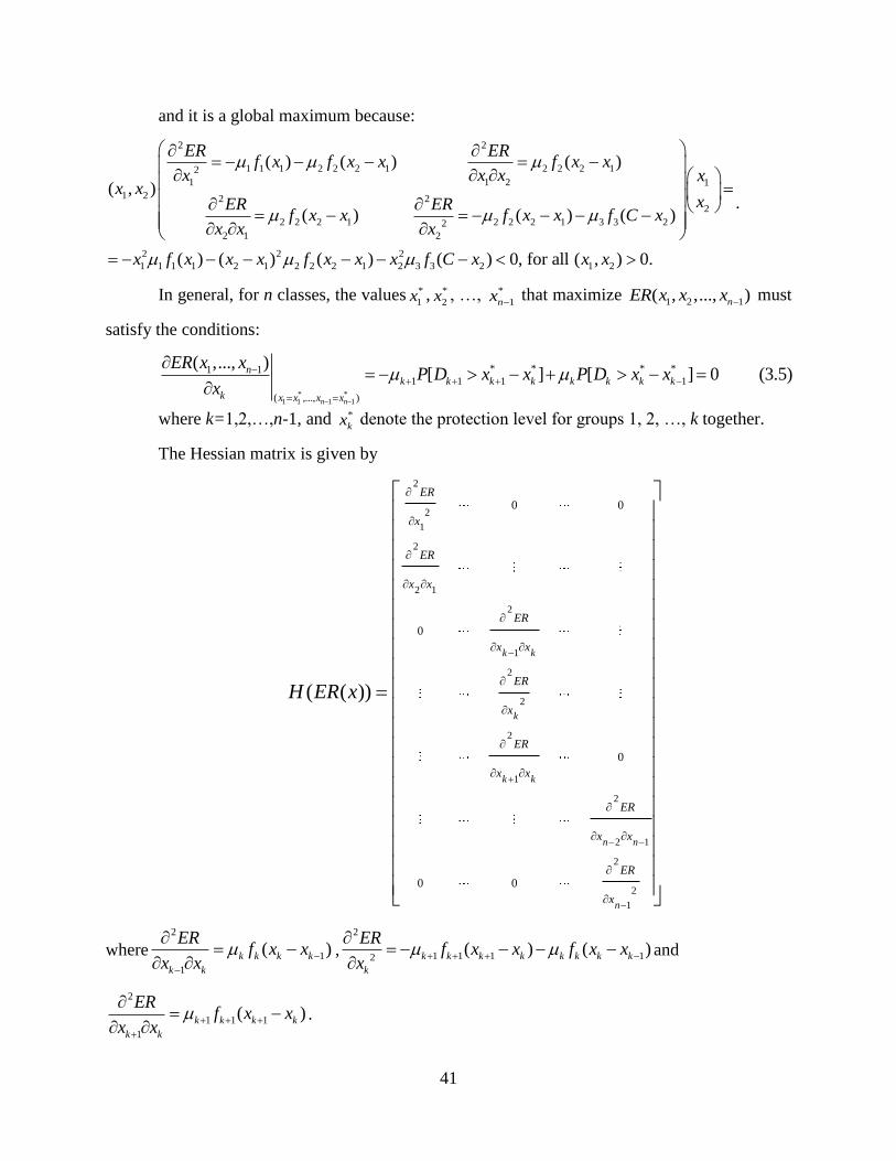
41
and it is a global maximum because:
2 2
1 1 1 2 2 2 1 2 2 2 12
1 1 2 1
1 2 2 22
2 2 2 1 2 2 2 1 3 3 22
2 1 2
2 2 2
1 1 1 1 2 1 2 2 2 1 2 3 3 2 1
( ) ( ) ( )
( , )
( ) ( ) ( )
( ) ( ) ( ) ( ) 0, for all (
ER ERf x f x x f x x
x x x xx x
xER ERf x x f x x f C x
x x x
x f x x x f x x x f C x x
2, ) 0.x
.
In general, for n classes, the values *
1x , *
2x , …, *
1nx that maximize
1 2 1( , ,..., )nER x x x must
satisfy the conditions:
* *1 1 1 1
* * * *1 11 1 1 1
( ,..., )
( ,..., )[ ] [ ] 0 (3.5)
n n
nk k k k k k k k
k x x x x
ER x xP D x x P D x x
x
where k=1,2,…,n-1, and *
kx denote the protection level for groups 1, 2, …, k together.
The Hessian matrix is given by
2
2
1
2
2 1
2
1
2
2
2
1
2
2 1
2
2
1
0 0
0
0
0 0
( ( ))
k k
k
k k
n n
n
ER
x
ER
x x
ER
x x
ER
x
ER
x x
ER
x x
ER
x
H ER x
where
2
1
1
( )k k k k
k k
ERf x x
x x
,
2
1 1 1 12( ) ( )k k k k k k k k
k
ERf x x f x x
x
and
2
1 1 1
1
( )k k k k
k k
ERf x x
x x
.

42
Because
2 2 2 2 2 2 222 2 2
1 1 2 1 1 1 2 12 2 221 2 1 1 1 2 1 1
12 2 2
1 1 1 1 1 1 1 1
1
' ( ( ))
( ) ( ) ( ) (
n
k k k k k n n n
k k k k k k n n n
n
k k k k k n n n n
k
x H ER x x
ER ER ER ER ER ER ERx x x x x x x x x x x
x x x x x x x x x x x
x f x x x f x x x f C x
1 2 1) 0, for all ( , ,..., ) 0,nx x x
H is negative definite, hence the solution to the system of equations (3.5) is a global maximum.
Case 2: None of the groups‟ demand would exhaust the system capacity, except the class that
contributes the least would, so that the capacity allocation problem is nontrivial.
Let n = 3, i.e., three classes. We assume that 1x is the capacity allocated to group 1 and
2x is
the capacity allocated to groups 1 and 2 together. The total expected revenue takes now into
account all 3! = 6 possible orderings among the 'iQ s and their probabilities
1 2 3 1 2 3( )i i i i i iP Q Q Q .
1 2 3 1 2 3 1 2 3
1 3 2 1 3 2 1 3 2
2 1 3 2 1 3
1 2 123 1| 1 1 2| 2 2 1 3| 2
132 1| 1 1 2| 2 1 3| 3 2
213 1| 1 1 2|
( , ) min{ , } min{ , ) ( )
min{ , } ( ) min{ , }
min{ , } mi
Q Q Q Q Q Q Q Q Q
Q Q Q Q Q Q Q Q Q
Q Q Q Q Q Q
ER x x E D x D x x C x
E D x x x D C x
E D x
2 1 3
2 3 1 2 3 1 2 3 1
3 1 2 3 1 2 3 1 2
3 2 1
2 2 1 3| 2
231 1| 1 2| 2 2 1 3| 3 2
312 1| 1 1 2| 2 1 3| 3 2
321 1| 1
n{ , } ( )
min{ , } min ,
min{ , } ( ) min{ , }
Q Q Q
Q Q Q Q Q Q Q Q Q
Q Q Q Q Q Q Q Q Q
Q Q Q
D x x C x
E x D x x D C x
E D x x x D C x
E x
3 2 1 3 2 12| 2 2 1 3| 3 2min{ , } min{ , } .Q Q Q Q Q QD x x D C x
1 2 1
1 2 3 1 2 3 1 2 3
1
1 3 2 1 3 2
1 2
123 1| 1 1 1 1 2| 2 2 1 2 2 1 3| 2
0 0
132 1| 1 1 1 1 2| 2 1 3
0
( , )
( ) [ ] ( ) ( ) [ ] ( )
( ) [ ] ( )
x x x
Q Q Q Q Q Q Q Q Q
x
Q Q Q Q Q Q
ER x x
yf y dy x P D x yf y dy x x P D x x C x
yf y dy x P D x x x
2
1 3 2
1 2 1
2 1 3 2 1 3 2 1 3
2 3 1
| 3 2 3 2
0
213 1| 1 1 1 1 2| 2 2 1 2 2 1 3| 2
0 0
231 1| 1 2
( ) ( ) [ ]
( ) [ ] ( ) ( ) [ ] ( )
C x
Q Q Q
x x x
Q Q Q Q Q Q Q Q Q
Q Q Q
yf y dy C x P D C x
yf y dy x P D x yf y dy x x P D x x C x
x
2 1 2
2 3 1 2 3 1
1 2
3 1 2 3 1 2 3 1 2
| 2 2 1 2 2 1 3| 3 2 3 2
0 0
312 1| 1 1 1 1 2| 2 1 3| 3
0 0
( ) ( ) [ ] ( ) ( ) [ ]
( ) [ ] ( ) ( ) (
x x C x
Q Q Q Q Q Q
x C x
Q Q Q Q Q Q Q Q Q
yf y dy x x P D x x yf y dy C x P D C x
yf y dy x P D x x x yf y dy C
2 1 2
3 2 1 3 2 1 3 2 1
2 3 2
321 1| 1 2| 2 2 1 2 2 1 3| 3 2 3 2
0 0
) [ ]
( ) ( ) [ ] ( ) ( ) [ ]
x x C x
Q Q Q Q Q Q Q Q Q
x P D C x
x yf y dy x x P D x x yf y dy C x P D C x

43
1 2 3 1 2 3 1 3 2 1 3 2
2 1 3 2 1 3 2 3 1 2 3 1
3 1 2
1 2
1
123 1| 1 1 2| 2 2 1 132 1| 1 1 2|
213 1| 1 1 2| 2 2 1 231 1| 2| 2 2 1
312 1|
( , )
[ ] [ ] [ ]
( ) [ ] [ ]
Q Q Q Q Q Q Q Q Q Q Q Q
Q Q Q Q Q Q Q Q Q Q Q Q
Q Q Q
ER x x
x
P D x P D x x P D x
P D x P D x x P D x x
3 1 2 3 2 1 3 2 1
1 2 3 1 3 2 2 1 3 3 1 2
1 2 3 2 1 3 2 3 1 3
1 1 2| 321 1| 2| 2 2 1
1 1 123 1| 132 1| 213 1| 312 1|
2 2 1 123 2| 213 2| 231 2| 321 2|
[ ] [ ]
[ ]
[ ]
Q Q Q Q Q Q Q Q Q
Q Q Q Q Q Q Q Q Q Q Q Q
Q Q Q Q Q Q Q Q Q Q
P D x P D x x
P D x
P D x x
2 1
1 3 2 2 3 1 3 1 2 3 2 1132 2| 231 1| 312 2| 321 1| 0
Q Q
Q Q Q Q Q Q Q Q Q Q Q Q
1 2 3 1 2 3 1 3 2 1 3 2
2 1 3 2 1 3 2 3 1 2 3 1
3 1 2
1 2
2
123 2| 2 2 1 3| 132 2| 3| 3 2
213 2| 2 2 1 3| 231 2| 2 2 1 3| 3 2
312 2| 3|
( , )
[ ] [ ]
[ ] [ ] [ ]
Q Q Q Q Q Q Q Q Q Q Q Q
Q Q Q Q Q Q Q Q Q Q Q Q
Q Q Q
ER x x
x
P D x x P D C x
P D x x P D x x P D C x
3 1 2 3 2 1 3 2 1
1 2 3 2 1 3 2 3 1 3 2 1
1 3 2 2 3 1 3 1 2
3 2 321 2| 2 2 1 3| 3 2
2 2 1 123 2| 213 2| 231 2| 321 2|
3 2 132 3| 231 3| 312 3|
[ ] [ ] [ ]
[ ]
[ ]
Q Q Q Q Q Q Q Q Q
Q Q Q Q Q Q Q Q Q Q Q Q
Q Q Q Q Q Q Q Q Q
P D C x P D x x P D C x
P D x x
P D C x
3 2 1
1 2 3 1 3 2 2 1 3 3 1 2
321 3|
123 3| 132 2| 213 3| 312 2| 0
Q Q Q
Q Q Q Q Q Q Q Q Q Q Q Q
The value of1x and
2x that maximize 1 2( , )ER x x , denoted by *
1x and *
2x , must satisfy the
conditions:
1 2 1 2
1 2
( , ) ( , )0 and 0
ER x x ER x x
x x
, i.e.,
2 3 1 3 2 1
1 3 2 3 1 2
* *
1 1 1 231 1| 321 1| 1 1
* * * *
2 2 2 1 132 2| 312 2| 2 2 1
[ ] 1 [ ]
[ ] 1 [ ]
Q Q Q Q Q Q
Q Q Q Q Q Q
P D x P D x
P D x x P D x x
and (3.6)
1 3 2 3 1 2
1 2 3 2 1 3
* * * *
2 2 2 1 132 2| 312 2| 2 2 1
* *
3 3 2 123 3| 213 3| 3 2
[ ] 1 [ ]
[ ] 1 [ ]
Q Q Q Q Q Q
Q Q Q Q Q Q
P D x x P D x x
P D C x P D C x
* *
1 2( , )x x is a global maximum because:
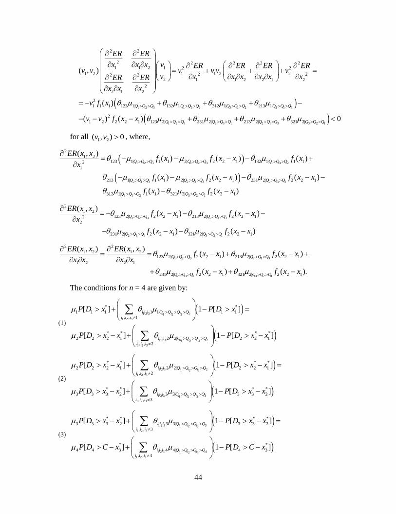
44
1 2 3 1 3 2 3 1 2 2 1 3
2 2
2 2 2 2 21 1 2 1 2 2
1 2 1 1 2 22 22 22 1 1 2 2 1 2
2
2 1 2
2
1 1 1 123 1| 132 1| 312 1| 213 1|
( , )
( ) Q Q Q Q Q Q Q Q Q Q Q Q
ER ER
x x x v ER ER ER ERv v v v v v
v x x x x x xER ER
x x x
v f x
1 2 3 2 3 1 2 1 3 3 2 1
2
1 2 2 2 1 123 2| 231 2| 213 2| 321 2|( ) ( ) 0Q Q Q Q Q Q Q Q Q Q Q Qv v f x x
for all 1 2( , ) 0v v , where,
1 2 3 1 2 3 1 3 2
2 1 3 2 1 3 2 3 1
3 1 2 3 2 1
2
1 2123 1| 1 1 2| 2 2 1 132 1| 1 12
1
213 1| 1 1 2| 2 2 1 231 2| 2 2 1
312 1| 1 1 321 2| 2 2 1
( , )( ) ( ) ( )
( ) ( ) ( )
( ) ( )
Q Q Q Q Q Q Q Q Q
Q Q Q Q Q Q Q Q Q
Q Q Q Q Q Q
ER x xf x f x x f x
x
f x f x x f x x
f x f x x
1 2 3 2 1 3
2 3 1 3 2 1
2
1 2123 2| 2 2 1 213 2| 2 2 12
2
231 2| 2 2 1 321 2| 2 2 1
( , )( ) ( )
( ) ( )
Q Q Q Q Q Q
Q Q Q Q Q Q
ER x xf x x f x x
x
f x x f x x
1 2 3 2 1 3
2 3 1 3 2 1
2 2
1 2 1 2123 2| 2 2 1 213 2| 2 2 1
1 2 2 1
231 2| 2 2 1 321 2| 2 2 1
( , ) ( , )( ) ( )
( ) ( ).
Q Q Q Q Q Q
Q Q Q Q Q Q
ER x x ER x xf x x f x x
x x x x
f x x f x x
The conditions for n = 4 are given by:
(1)
1 2 3 11 2 3
1 2 3
1 2 3 21 2 3
1 2 3
* *
1 1 1 1 1| 1 1
, , 1
* * * *
2 2 2 1 2 2| 2 2 1
, , 2
[ ] 1 [ ]
[ ] 1 [ ]
i i i
i i i
i i i Q Q Q Q
i i i
i i i Q Q Q Q
i i i
P D x P D x
P D x x P D x x
(2)
1 2 3 21 2 3
1 2 3
1 2 3 31 2 3
1 2 3
* * * *
2 2 2 1 2 2| 2 2 1
, , 2
* * * *
3 3 3 2 3 3| 3 3 2
, , 3
[ ] 1 [ ]
[ ] 1 [ ]
i i i
i i i
i i i Q Q Q Q
i i i
i i i Q Q Q Q
i i i
P D x x P D x x
P D x x P D x x
(3)
1 2 3 31 2 3
1 2 3
1 2 3 41 2 3
1 2 3
* * * *
3 3 3 2 3 3| 3 3 2
, , 3
* *
4 4 3 4 4| 4 3
, , 4
[ ] 1 [ ]
[ ] 1 [ ]
i i i
i i i
i i i Q Q Q Q
i i i
i i i Q Q Q Q
i i i
P D x x P D x x
P D C x P D C x

45
and in general we have:
1 2 1 11 2 1
1 2 1
1 2 1 1 2 1
1 2 1
* * * *
1 1 1 2 ... 1 1| ... 1 1 2
, ,..., 1
* * *
1 ... | ...
, ,...,
[ ] 1 [ ]
[ ] 1 [
n i i i kn
n
n i i i kn
n
k k k k i i i k k Q Q Q Q k k k
i i i k
k k k k i i i k k Q Q Q Q k k
i i i k
P D x x P D x x
P D x x P D x
*
1] (3.7)kx
* *
0for =2,3,...,n, with and 0.nk x C x
These conditions can be re-written as:
1 2 1 1 1 1 2 11 2 1 1 2 1
1 2 11 2 1
1 2 1 1 2 1
* *
..., , 1| ... ..., , 1| ... 1 1 2, ,..., ,, ,..., 1
1
..., , | ...
[ ]n k i i i k n n i i i in n n
n nn
n
n k i i i kn
i i i i k Q Q Q Q i i i i k Q Q Q Q k k ki i i ii i i k
i k
i i i i k Q Q Q Q
P D x x
* *
0
1 2 1 1 2 1
1 2 11 2 1
* *
..., , | ... 1, ,..., ,, ,...,
for 2, ..., , with and 0.
[ ]
n
n n i i i in n
n nn
n
i i i i k Q Q Q Q k k ki i i ii i i k
i k
k n x C x
P D x x
(3.8)
Note that 1 2 1 1 2 1
1 2 1
..., , | ...
, ,...,n k i i i kn
n
i i i i k Q Q Q Q
i i i k
represents the expected marginal
contribution of class k to the total expected revenue when it is the class that contributes the least,
and 1 2 1 1 2 1
1 2 1
..., , | ..., ,..., ,
n n i i i in n
n n
n
i i i i k Q Q Q Qi i i i
i k
represents the expected marginal contribution of class k
to the total expected revenue when it is not the class that contributes the least. It is easy to see
that if we only have two classes, (3.8) becomes (3.4). To be also noted that if
* , 1,..., 1kx C k n , then there is no available resource to be protected during the next booking
period for 1,...,k n classes, and that the requests coming from these last classes need to be
postponed until a later booking period.
Individual customer resource requirements in service applications, such as legal aid or
health-care, may be highly variable even though services must be sold on a fixed-price basis. The
resources each service uses are known exactly only after the service is performed, adding to the
complexity of the resource allocation decisions. Cost and managerial pressures may require those

46
environments to be sensitive to revenue management considerations, making the results we
derive in this work of considerable practical interest.
Our analyses follow the established criterion of setting the protection level so as to
maximize the expected return. When individual resource requirements, as well as demand levels,
are uncertain, selecting a protection level might be based, in practice, on an explicit recognition
of the variance of return and not just on its expectation. The expected return and its variance
could be used to construct an efficient frontier, with the decision maker choosing an appropriate
point on that efficient frontier based on risk tolerance.
The results presented above help the decision maker identify the optimal allocation of a
scarce resource (e.g., service time, working space, etc.) across multiple customer classes, to
maximize the expected revenue when the individual service times are variable and customers‟
arrivals are random. When resource consumption is variable and known only after the service is
completed, it is risky to schedule a predetermined number of customers without running into
overtime. Our solution provides an optimal resource allocation across customer classes, and,
unlike more traditional scheduling work, it does not focus on offering a recipe on how many
customers from each class to service in each session. The scheduler can make informed, on the
spot decisions about scheduling or postponing a new customer based on his/her class
characteristics and his/her class‟ protection level.
47
4.0 REVENUE MANAGEMENT WITH RANDOM RESOURCE REQUIREMENTS:
APPLICATIONS IN HEALTHCARE
In this chapter we present the implementation of the optimization model in the healthcare arena,
and show the recommendations dictated by the model in terms of protection levels. We discuss
the complexity of the model, and show that some of the model‟s implementation difficulties
could be overcome by the use of a proposed heuristic. The chapter ends with a discussion about
overtime and its practical implications.
We report on both the optimal results and the ones obtained following a simulation model
created to mimic the situation described in the mathematical model. We use simulation for two
purposes: firstly, to show that simulation-based optimization can result in protection levels very
close to the theoretical optimal ones; secondly, to implement and show the performance of the
proposed heuristic for computing protection levels for any combination of elective surgery and
patient‟s reimbursement category, thus overcoming some of the model‟s complexities.
A surgical unit, having knowledge of these optimal protection levels (i.e., hours to be
protected for each type of surgery or subspecialty), could further decide on a policy for accepting
patients‟ requests for service and the sequence in which these requests are satisfied. Further, the
daily sequence of satisfying these requests can be analyzed using a bin packing algorithm that
can reduce the fixed costs of opening operating rooms, while maximizing expected contribution

48
during the planning horizon. There is a rich body of literature on the daily surgery scheduling, so
this last topic does not constitute our focus here.
Following the optimization model presented in Chapter 3 that models the problem of
managing patients‟ demand for service under variable resource usage considerations, we provide
computational results for both theoretical and simulation models. While the problem of patient
scheduling can be regarded as having two stages (protection level computation, followed by the
acceptance/rejection policy), we are mainly concerned here with the first stage, namely the
computation of optimal protection levels for classes of demand, and provide a heuristic for larger
scale problems, when optimal computations may become prohibitive.
4.1 PROBLEM SETTING OVERVIEW
From a broad perspective, this work addresses a service providing setting, in which requests for
elective surgeries by patients pertaining to various reimbursement categories translate into a
fluctuating demand for a relatively limited resource that is shared by multiple classes of
customers. The fluctuating demand has two sources of variation; first, the number of patients
from each class varies across time periods; second, patients‟ demand for a type of elective
surgery is dependent on the type of service (surgery) requested.
The common resource, time, is able to satisfy any type of service request and needs to be
allocated among these various customer classes. The resource replenishes at the beginning of
each period and it has a capacity of C time units available, with the possibility of limited
overtime, at some cost, usually higher than the cost for regular time. Starting with C units of
capacity, the surgical department begins receiving requests from patients for a type of service
(elective surgery). Even if we do not limit the analysis to any particular demand arrival
distribution, the Poisson process is a natural model to represent the arrival process of customers
with arrival rates that depend on class particularities, and, possibly, time during the day or week.

49
A request for service requires a number of units of resource (units of time) to be
allocated/diverted towards satisfying that request, dependent only on the service requested; if
accepted, it brings a revenue dependent on both the customer reimbursement category and
service type.
The decision on when to schedule each request for service or for how long to postpone it,
it is not that straightforward. The RM question, pertaining to the booking control and capacity
allocation components of RM practice, becomes: how many patients requests, from different
reimbursement categories, should the surgical unit accept, at most, for each type of service, and
whether or not each booking request received should be accepted or rejected. Before these
questions can be answered in the considered healthcare setting, we should first decide how many
units of time should be protected for higher paying customer classes (in expectation) and how
many time units should be protected, at most, for lower fare classes, with the final objective of
maximizing expected revenue/contribution margin. A customer‟s request for service at some
future date is accepted provided that there is capacity remaining to satisfy the request, and if the
total resource allocated for the previously accepted customers within that same class is less than
the protection level for that class. To be noted that here we refer to the protection levels as
partitioned, not as nested. In this sense, our protection levels are similar to the booking levels
mentioned in Chapter 2.
The standard single-leg RM setting, in which customers from various classes request
products pertaining to their fare-class for some future date, (seats in an airplane, rooms in a hotel,
etc.), assumes that capacity shared by all classes is fixed. While this is true in the aforementioned
cases, this assumption may not necessarily hold true all the time. This is especially the case of
those types of service in which the time to handle the accepted requests does not take exactly as
long as the norm states. Examples may include dental practices, where dental interventions may
take longer or shorter than initially estimated and planned for, auto-repairs, beauty salons,
diagnostic facilities within a hospital (MRI, CAT scans), and last, but not least, surgical
procedures.
The motivation of this work grew out of a keen observation that RM techniques can be
applied in service settings that exhibit variability with respect to service times. The managerial
decision from the hospital‟s standpoint is how much operating room capacity to reserve (book or
protect) in advance, to accommodate patients‟ requests for elective surgeries, when the patients

50
can be segmented based on a common characteristic (reimbursement or contribution level).
Because of the inherent variability in the service rendered, each accepted and scheduled request
for surgery will use up a variable amount of resource (time, in this case), which makes the
patient scheduling problem not a trivial one. We show how the optimal protection level results
developed in Chapter 3 are helping with this managerial decision of scarce (yet renewable)
resource allocation across surgical subspecialties during the planning horizon. While overtime is
allowed, too much overtime is not desired, because it usually comes at a much higher cost than
the use of resources during normal operating hours (Strum et.al., 1999). Following the
mathematical model and assumptions discussed in Chapter 3, overtime is not our main focus
here, but we discuss its implications.
The examples presented in this chapter follow the results discussed in the previous
chapter on surgical time allocation, considering demand and service time uncertainty, along with
arbitrary patient arrivals. The analysis incorporates the idea of accepting/postponing requests for
service from several competing classes of patients which present fluctuating demands. The
patients segmentation in various fare-classes is based on the contractual revenue expected to be
paid by each patient category. We can think of this segmentation in terms of patients‟ ability to
pay, rather than their willingness to pay (Karaesmen and Nakshin 2007).
Obtaining the optimal protection levels is of strategic importance for the surgical time
allocation across subspecialties, and for the tactical decision of determining the number of
patients‟ requests to be accepted from each fare-class and for each type of surgery in order to
maximize the expected revenue function over the planning horizon. This work tries to shed light
onto the applicability of some RM techniques and heuristics within a service setup that deals
with variable service time, and where customers have different degree of priority artificially
assigned to them based on their demand class.
51
4.2 HEALTHCARE APPLICATION - MOTIVATION
In order to cope with the increasing demand for healthcare, and particularly, surgical needs, a
surgical suite is required to efficiently balance a high usage rate of the operating room (OR)
while reducing the costs of utilization and maintaining or improving the quality of care. Besides
the challenges imposed by this increasing demand in a context of limited resources, another very
important factor which impedes the efficient use of existing resources is the variability in both
demand and service time. In an OR setting, this translates in both an uncertain number of patients
in need for surgery as well as inherent variability in the surgery time across types of surgeries,
surgeons and patients.
Inefficient OR scheduling may result in delays, or even cancellations, of surgeries or
other procedures, with a negative impact on hospital and patients. The patients suffer because a
delay or cancellation may be detrimental to his/her health condition with a negative effect on
quality of life in general. From the hospital perspective it may result in deferred or lost revenue
(in the situation where the surgery will be performed by another hospital or in another country
altogether), loss of goodwill, over and/or underutilization costs, just to mention the most obvious
ones. With its high operating costs, the surgical suite is known to potentially incur the highest
cost among the hospital‟s major areas. Reducing the operating costs and increasing the utilization
using a more efficient OR and patient scheduling were the focus of the largest OR literature. But
focusing on increasing the revenue from surgeries scheduling and OR utilization may become as
important as containing costs, because in the end, the survival and good functioning of any unit,
be it in manufacturing or healthcare, will depend on the financial soundness of that unit, and how
well it balances related costs and revenues.
When dealing with surgical scheduling, the term “scheduling” refers to two different
activities. Advanced scheduling refers to the activity which results in scheduling patients for
surgery at some day into the future. On the other hand, allocation scheduling results in
determining the exact order, or sequence, and times of surgeries performed in a day. Our
research focuses on advanced scheduling, in a hospital setup that normally operates on a FCFS
basis (non-block booking system).
In a first-come-first served patient booking policy, the system accepts requests from
patients as they occur, and the service is also provided in this manner. If there still are available

52
slots over the opened booking horizon, a request is assigned to a particular day in that horizon.
Only a couple of days before the surgery date, the schedule for that particular day is compiled
and all the surgeries scheduled for that day are assigned a starting time, usually function of
doctor‟s time preference and other resource availability.
In this work, we are not concerned with the OR daily schedule or procedure sequencing,
but rather to the booking decisions that lead to accepting or rejecting a particular request and
assigning it OR time during the open booking period, if accepted. The surgical procedures use up
a variable amount of time, and usually cannot be well confined within the allocated time slot -
hence, the over and underutilization of OR and doctor‟s time. This is also why we are looking at
the time resource as a continuum, rather than dividing it into the classical slots. Moreover, the
surgeries generate variable revenue per unit of time, function of the actual duration of the
procedure.
A medical bill is difficult to calculate exactly before the service takes place, but an
estimate could be obtained on the cost for service that the clinic/hospital would bill (and
potentially receive from) the patient and/or the patient‟s insurance company. Between these two
payment components, the latter is more certain, especially during the current economic
conditions when companies are starting to pass a larger share of the healthcare cost to their
employees, who would have to deal with a larger portion of their medical bill. Hospitals are
budgeting millions of dollars annually to cover losses from bad debt and/or unpaid medical bills.
This affects their bottom line profit and their capacity to have a sustainable growth to provide
long term care. This also leads to price increases for medical procedures, which, in turn, force
people to postpone treatment or look for it somewhere else, usually abroad – phenomenon called
medical tourism.
Surgical departments are profit units within a hospital and should function as such.
Accepting all requests for elective surgeries or procedures could be seen as having a downside
under the current economic conditions, and postponing some requests may be in order if it helps
the financial position of the hospital.
Our work analyzes these accept/postpone decisions and offer a booking policy that would
benefit the profitability of the medical institution, which in turn will help provide better long
term care. Reserving/protecting operating room capacity (time) based on the patient class
53
(surgery type and insurance level) brings the revenue management perspective and theory into
the patient appointment scheduling arena.
We follow the theory developed in Chapter 3 on computing protection levels under the
assumption of random resource utilization per service. We show how this booking policy
behaves in the medical setting when dealing with patients‟ requests for elective surgeries. The
policy allows the decision maker to decide how much time, over the booking horizon, to protect
in a nested or partitioned fashion for the various categories of patients who call for service, and
whether a request should be immediately accepted and included in the schedule or postponed for
a future booking horizon.
4.3 PROBLEM STATEMENT IN THE OPERATING ROOM SETTING
Our work is concerned with the advanced scheduling of patients for elective surgery when the
operating room capacity usage by these elective procedures is uncertain. We study the
application of some revenue management techniques to scheduling operating rooms for a variety
of common surgical procedures performed in a multi-tier reimbursement system. Our approach
to the problem is focusing only on booking requests for elective procedure, but since emergency
patients have priority over all other patients, always creating some disruption in the initial
schedule, we also touch on this issue in the conclusions chapter.
New requests for bookings for elective surgeries arrive each day from patients, based on
their doctors‟ recommendations. Under unconstrained capacity conditions, these procedures
would be performed as soon as possible, but in reality OR capacity is limited in a given day,
considering the number of available doctors, nurses, equipment etc, so accepting too many
requests for a certain day or time period will, in most cases, result in excessive overtime, or even
turning away previously scheduled patients or emergency cases. An additional difficulty arises
from the fact that the exact time it takes to perform various elective surgical procedures is not
known with certainty at the time of booking (Shukla, Ketcham et al. 1990). The problem the
hospital faces in general, and the surgery scheduling department in particular, at the beginning of
each day (planning period or booking window), is to decide how many of the additional requests

54
for elective surgery to accept for that day and for the days to come, for which the booking
process is open, with the goal of maximizing the expected revenue but without disregard to
regular and overtime utilization.
We start by implementing the model described in Chapter 3 using realistic data, either
simulated or historical, to answer the question of how much time should optimally be protected
for various classes of patients during the planning period. Later, we implement an adapted RM
heuristic that would help the decision maker deal with the complexity of the optimal
computations. These optimal (or close to optimal) protection levels would further help the
decision maker with identifying the actual number of elective surgeries to accept, at most, for
each class of patient that will maximize expected contribution.
The results obtained in Chapter 3 can be used to implement an advance dynamic booking
policy. The protection levels are computed using forecasted demand for the next planning period,
which is based on historical demand distribution for each type of surgery. The distribution of the
reimbursement category is assumed to follow the national distribution of the main insurance
categories, but each institution is free to use the distribution that better fits its market demand.
These demand distributions will be updated as the time horizon progresses, at intervals that
would make sense to suspect that there are major changes/shifts in the demand distributions.
We assume that the hospital has evidence and past records of all past requests for elective
surgeries, including those that were not finally honored (patient either gave up, died, or went to a
different hospital). This assumption avoids the censoring realizations of demand situations that
are so common in airline or hotel industry (Van Ryzin and McGill 2000), where it is very
difficult to keep track of every unfilled request that was made online, for example. If a lost
demand occurs, the management may not know about it. But in the hospital environment, where
requests for surgery are taken by a receptionist/scheduling personnel, should be realistic to
assume that there is a complete or large enough set of records of all past requests.
Unlike previous research where priority classes usually correspond to the degree of
urgency for the procedure, in the present study the priority classes correspond to the expected
revenue per unit of time expected to be obtained by performing a procedure on a patient from
that class. Following this, it is not always true that higher patient classes would correspond to
patients that have full health insurance/coverage, while lower priority classes correspond to
classes of patient that have low or no health insurance. The expected revenue per unit of time

55
dictates the rankings across classes, where both the revenue per surgery and the surgery
durations are influencing factors. For this reason, two hospitals practicing the same prices, but
where surgeons performing those surgeries differ in their effectiveness, may have different
rankings for those patient classes, resulting in different optimal protection levels. This means that
surgeon‟s efficiency and effectiveness are direct factor influencing the optimal protection levels.
This choice of patient segmentation, based on the reimbursement category (insurance
coverage level) for the type of procedure requested lends itself naturally to analyzing and
formulating the problem as one of expected revenue maximization, as presented in the previous
chapter. The segmentation makes sense when considering the harsh economic realities of
managed care, in which medical institutions must manage surgical services efficiently to contain
costs and ensure their own survival.
Most models in the related literature deal with computing performance measures for the
proposed control policies, like average utilization, patients and resources waiting time, waiting
queue length, etc (see, e.g. Taylor and Templeton (1980), Rege and Sengupta (1996)). Rather
than computing performance measures for various policies, we are computing the optimal
protection levels that lead to maximizing the expected revenue for the surgical department.
4.4 DATA SUMMARY
The data used in this work consist of records of all surgical cases performed at a large teaching
hospital over a six year period from 1989 to 1995. Independent variables in the data were
surgical procedures by date, patient birth-date and gender, type of anesthesia, emergency status,
anesthesia start time, surgical preparation time, surgical start time, surgical end time, anesthesia
end time, CPT code (Common Procedural Terminology), anesthesiologist, surgeon, and
admission status (inpatient vs. outpatient). All cases were evaluated by the surgical subspecialty
blocks to which they were assigned. Use of the anonymous patient record was approved by the
human subjects review committee of the institution which collected the data.
The initial data consisted of more than 50,000 records of surgical cases obtained over
1,591 weekdays or 328 weeks, from 9-18 operating suites daily. There were 5,122 different CPT

56
coded procedures of which 3,166 procedures occurred 2 or more times. A closer analysis of the
original data led to the elimination of incomplete records and CPTs with less than 5 records.
Surgeries with more than 2 CPTs were labeled according to the first CPT listed. After all the data
manipulations, our final database includes the 53 most representative CPTs (with most records)
across 20 subspecialties, totaling 15,886 records. For the purpose of this research, we were
mostly interested in the total surgical time for each record, as well as the number of surgeries that
were performed on a daily basis. The surgical duration helped us identify and fit appropriate
distributions, while the daily number of surgeries of each type helped us recreate the daily and
weekly demand in terms of both number of surgeries and total duration. We fitted the 2-
parameter lognormal distribution for all the 53 CPTs, resulting in 4 out of 53 (7.5%) of the CPTs
to fail the log-normality test at = 0.05.
Table 1 below includes the nomenclature of the 20 subspecialties represented by the 53
CPT data. It is followed by Table 2, which summarizes the CPT data and the parameters of the
lognormal distributions fitted to the data.
Table 1: Subspecialty nomenclature
1 = Intergumentary 6 = Chest 11 = Laparoscopic 16 = Eye and Adnexa
2 = Muskuloskeletal 7 = Digestive 12 = Female Genital 17 = Auditory
3 = Respiratory 8 = Urinary 13 = Maternity Care 18 = Radiology
4 = Cardiovascular 9 = Male Genital 14 = Endocrine 19 = Pathology
5 = Hematology 10 = Intersex 15 = Nervous system 20 = Medicine

57
Table 2: Surgical data description

58
4.5 RANDOM RESOURCE REQUIREMENTS: APPLICATION RESULTS
The problem associated with OR time inventory control is determining the protection levels for
each class of patients that will maximize the total expected revenue for the surgical unit over a
certain time horizon (scheduling period). These protection levels can be thought of as time
partitions, in the sense that the results obtained following our model dictate how much time to
allocate for each patient class, defined as surgery type – health coverage level combination.
The results obtained in Chapter 3 can be used in practice to create either a static or
dynamic inventory (time) control, depending on the demand information available and the
frequency of updating the protection levels as a function of the level of accuracy desired by the
decision maker. The model looks to set time protection levels with respect to each insurance
level within each surgery type at the start of the scheduling period using the total demand
forecasted for each surgery-insurance combination.
When the forecast is used at the beginning of the scheduling period and the protection
levels are not updated, we are in the situation of the static model. If, on the other hand, the
forecast are updated as new demand information becomes available, resulting in more frequently
updated protection levels, then we are under the dynamic inventory control situation. This latter
situation naturally accounts for cancelations and no-shows. If we deal with a dedicated OR, for
example, where only one surgery is performed most of the time, the model will dictate how
much time should be allocated (reserved) for patients covered by different health insurance
levels in need for that particular surgery. As new information about demand becomes available,
these protection levels can be updated, thus leading to more appropriate and close to optimal
protection levels (dynamic situation).
Our model does not make any assumptions about the order of patients‟ arrival. That is,
we assume random customer arrivals, which stochastic total demand per customer class. This
mimics what happens in practice, where customers from different classes arrive based on needs,
concurrently rather than sequentially, and not necessarily in some order determined by their
reimbursement category. All patients‟ requests for surgery type j possessing insurance level i
constitute class ij‟s demand. Hence, a class‟ demand is function of the surgery j‟s duration and
the fraction of patients holding type i insurance coverage. The information can be obtained by
analyzing historical data on past surgeries of that type performed in that surgical unit or medical

59
facility, and by analyzing historical data and forecasts about the population structure on surgery
needs and insurance coverage.
Our data come from a large teaching hospital, as presented previously, and include six
years worth of data pertaining to a plethora of surgeries performed during this time. The
parameters of the fitted distributions were presented in Table 2. The information on the actual
cost incurred and revenue generated by the surgeries performed is not available, because it was
not recorded when the surgeries took place. To compensate for this, we make some assumptions
on the relative values between the revenue generated by a surgery of type j when requested by a
patient holding an insurance coverage (reimbursement category) plan type i, which generates a
price ijp to be reimbursed to the hospital for the service performed. Another drawback following
the lack of the actual values for some of the input parameters and results, resides in the
impossibility of calculating the revenue increase when applying the optimal protection levels
versus the status quo situation.
We assume that we can establish an ordering between the revenues generated per type of
surgery by patients holding different insurance types, and that the more comprehensive the
insurance plan that the patient has, the more revenue is guaranteed to be reimbursed to the
surgical unit. But as each surgery takes a variable amount of time, the revenue generated per unit
of time will vary even across same type surgeries. While this adds to the difficulty of OR time
allocation across surgical types, we also assume that is possible to rank (order) the revenues per
time unit generated by various classes of patients.
The results presented in the previous chapter show the optimal time allocation between
several competing customer (patient) classes, when the operating unit has a fixed capacity during
the planning horizon. The resource allocation policy applies equally well when planning horizon
is a day (8-12 hours), a week, or more. The mathematical results determine the optimal
protection levels, which, when implemented, lead to maximizing expected revenue over that
booking window.
Next, we show that theoretical optimal protection levels could be closely matched by
ones obtained using optimization through simulation. We present several examples using both
simulation (using Crystal Ball simulation package, 11th
edition) and Mathematica (Wolfram
Mathematica 7.0.0) to show that the simulation results closely agree with the theoretical one, and
to discuss the reasons behind the slight differences that could occur between these results. While

60
for a relatively small number of classes computing the optimal protection levels following the
mathematical model it is straightforward (here using Wolfram Mathematica version 7.0.), when
the number of classes increases, obtaining the necessary input parameters needed for Case 2
leads to computational difficulties, as we will explain later, in the “Computational Complexity”
subchapter. For the situation when the problem becomes large, we propose a heuristic for
computing close to optimal protection levels within a reasonable timeframe.
The simulation model is set up to closely mimic the situation and assumptions in the
mathematical model. A random number of patients are arriving each day. They could be either
completely new arrivals, or postponed from the previous booking periods. Their inter-arrival
time is considered to be very small, only large enough to create a sequence among those
customers requesting service. As a patient arrives, (s)he gets assigned a surgical duration (jt ),
drawn from the probability distribution fitted on the historical data on that type of surgery. The
patient also gets assigned a class, (i =1,2,3,…,n) with probability ir , based on the insurance type
(s)he possesses. This also establishes the potential revenue generated by that patient,ijp .
In the case where all patients demand the same type of elective surgery over the planning
horizon, j=1. We analyze this situation first. Let N be the number of total patients requesting
service for the next booking period. Only a subgroup will be scheduled for this next period,
based on each class‟ corresponding protection level, ix . The protection level for class 1 patients,
for example, 1x , defined as the number of time units reserved at the beginning of each time
period exclusively for class 1, could be expressed either in time units (minutes, hours) or as a
percentage of capacity, C. Then 1C x is the maximum time available for the other classes of
patients during the scheduling time frame. Since we analyze partitioned protection levels, an
additional class 1 patient will be scheduled for that booking window if the projected surgery time
for this new patient fits within the remaining time for class 1 protection level. Similarly, an
additional class i patient will be scheduled for that period if the time projected for this new
patient fits within the remaining time for class i’s protection level, 1i ix x , following the
notation used in the mathematical model. Each class i patient scheduled for that timeframe brings
in a revenueip , so that
1 1i i ip p p .
Following the mathematical model and results described in the previous chapter, we are
presenting several examples to illustrate the implementation of the model, using both fictitious

61
and real data. In what follows, we assume that requests for surgery are coming from patients
segmented in 2 and then 3 categories based on their insurance type.
4.5.1 Case 1
4.5.1.1 Two classes
The mathematical model analyzed under Case 1 for two classes (see Chapter 3) includes
situations in which 1 2 1 21, 1, 1P D C P D C P D D C
Example 1: Capacity (C) = 8 hrs/day, p1=$1, p2=$0.6 (p1/p2=1.667), surgery time follows
a 2-parameter Lognormal (=1.4, =0.6), probability class 1, r1= 40% (r2=60%), maximum
arrivals/day = 15, 1 = 0.83 and
2 = 0.5 are the contributions per unit of time (per hour), the
empirical D1 and D2 are normally distributed with mean and standard deviations of 4.35 hours
and 1.68 hours for class 1, and 5.46 hours and 1.6 hours for class 2 respectively. Based on (3.3),
let‟s define Difference = 1 1 2 2 . P D x P D C x
The graph below plots the simulation-based optimization results: Expected Total
Revenue (ETR) on the secondary Y axis (right), and the Difference on the main Y axis (left) vs.
61 values for the simulation-based optimal protection levels, expressed as percentage of capacity.
It can be observed that the protection level following the simulation-based optimization
(x = 4.08 hrs = 51% of C) for which ETR is maximized ($3.733) also satisfies (3.3), almost
exactly; it is satisfied exactly for x = 4.16 hours (52% of C). The theoretical optimal protection
level (computed using Mathematica), assuming a normal demand with the parameters above, is x
= 4.27 hours (53.4% of capacity), only 2.6% larger than the one obtained using simulation-based
optimization. A polynomial trend was fitted to the simulated revenues, along with the coefficient
of determination R2, showing the concavity of the expected revenue function.
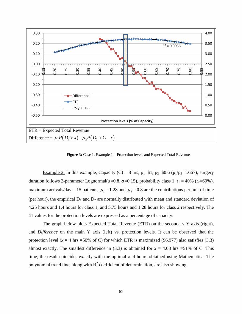
62
ETR = Expected Total Revenue
Difference = 1 1 2 2 . P D x P D C x
Figure 3: Case 1, Example 1 – Protection levels and Expected Total Revenue
Example 2: In this example, Capacity (C) = 8 hrs, p1=$1, p2=$0.6 (p1/p2=1.667), surgery
duration follows 2-parameter Lognormal(=0.8, =0.15), probability class 1, r1 = 40% (r2=60%),
maximum arrivals/day = 15 patients, 1 = 1.28 and
2 = 0.8 are the contributions per unit of time
(per hour), the empirical D1 and D2 are normally distributed with mean and standard deviation of
4.25 hours and 1.4 hours for class 1, and 5.75 hours and 1.28 hours for class 2 respectively. The
41 values for the protection levels are expressed as a percentage of capacity.
The graph below plots Expected Total Revenue (ETR) on the secondary Y axis (right),
and Difference on the main Y axis (left) vs. protection levels. It can be observed that the
protection level (x = 4 hrs =50% of C) for which ETR is maximized ($6.977) also satisfies (3.3)
almost exactly. The smallest difference in (3.3) is obtained for x = 4.08 hrs =51% of C. This
time, the result coincides exactly with the optimal x=4 hours obtained using Mathematica. The
polynomial trend line, along with R2 coefficient of determination, are also showing.
R² = 0.9936
0.00
0.50
1.00
1.50
2.00
2.50
3.00
3.50
4.00
-0.50
-0.40
-0.30
-0.20
-0.10
0.00
0.10
0.20
0.30
0.1
5
0.2
0
0.2
5
0.3
0
0.3
5
0.4
0
0.4
5
0.5
0
0.5
5
0.6
0
0.6
5
0.7
0
0.7
5
0.8
0
0.8
5
Protection levels (% of Capacity)
Difference
ETR
Poly. (ETR)

63
ETR = Expected Total Revenue
Difference = 1 1 2 2 . P D x P D C x
Figure 4: Case 1, Example 2 – Protection levels and Expected Total Revenue
Example 3: In this example, Capacity (C) = 9 hrs, p1=$1, p2=$0.6 (p1/p2=1.667), surgery
duration follows a 2-parameter Lognormal (=1.1, =0.2), probability class 1, r1 = 40%
(r2=60%), maximum arrivals/day = 15 patients, 1 = 0.94 and
2 = 0.56, empirical demands are
normally distributed, with mean and standard deviation of 5.37 and 1.82 hours for class 1, and
6.7 and 1.5 hours for class 2, respectively . The graph below plots Expected Total Revenue
(ETR) on the secondary Y axis (right), and Difference on the main Y axis (left) vs. 33 values for
the simulation-based optimal protection levels.
In this example, it can be observed that simulation resulted in two protection levels, one
satisfying the maximum expected revenue requirement (x = 5.58 hours =62% of C) which results
in a difference of -0.12 for Difference, one satisfying Difference, (x=5 hours = 56% of C), which
results in a 1.6% difference in expected total revenue. This is mainly due to randomness, even
when a large number of simulation runs was performed (we used 5000 simulation runs). By
plotting the polynomial trend-line, we can see that the maximum expected revenue should have
been obtained for the same protection level which satisfies Difference, i.e., x=5 hours = 56% of
R² = 0.9541
6.20
6.30
6.40
6.50
6.60
6.70
6.80
6.90
7.00
7.10
-0.8
-0.6
-0.4
-0.2
0
0.2
0.4
0.60
.35
0.4
0
0.4
5
0.5
0
0.5
5
0.6
0
0.6
5
0.7
0
0.7
5
0.8
0
0.8
5
Protection levels (% of Capacity)
Difference
ETR
Poly. (ETR)

64
C. This result is the optimal one, obtained with Mathematica. That is, the surgical unit should
reserve/protect 5 hours out of the 9 available for that day for class 1 patients.
ETR = Expected Total Revenue
Difference = 1 1 2 2 . P D x P D C x
Figure 5: Case 1, Example 3 – Protection levels and Expected Total Revenue
4.5.1.2 Multiple classes
We are now discussing how the mathematical model is actually put in practice when dealing
with patients‟ requests for multiple surgeries, thus having multiple classes. How do we move
from a solution that assumed one service being provided, to a series of surgeries that need to be
performed during the planning horizon? When the surgical department needs to schedule
patients, which could have one of the “i” reimbursement categories, for 2j surgeries, it comes
down to computing n-1 optimal protection levels across the n=i*j total classes by solving a
system of n-1 simultaneous equations.
Let ijp be the revenue generated by a patient having class i insurance level, and
requesting surgery type j, and ij
ij
j
pQ
T be the revenue per unit of time contributed by the same
R² = 0.8693
5.30
5.35
5.40
5.45
5.50
5.55
5.60
5.65
5.70
5.75
5.80
5.85
-0.40
-0.30
-0.20
-0.10
0.00
0.10
0.20
0.30
0.4
3
0.4
5
0.4
7
0.4
9
0.5
1
0.5
2
0.5
4
0.5
6
0.5
8
0.6
0
0.6
2
0.6
4
0.6
6
0.6
8
0.7
0
0.7
2
0.7
4
Protection levels (% of Capacity)
Difference
ETR
Poly. (ETR)
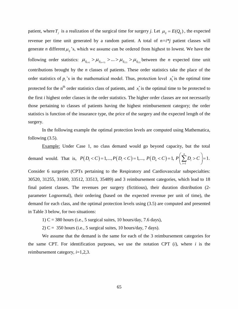
65
patient, wherejT is a realization of the surgical time for surgery j. Let ( )ij ijE Q , the expected
revenue per time unit generated by a random patient. A total of n=i*j patient classes will
generate n differentij ‟s, which we assume can be ordered from highest to lowest. We have the
following order statistics: ( ) ( 1) (2) (1)
...n nij ij ij ij
between the n expected time unit
contributions brought by the n classes of patients. These order statistics take the place of the
order statistics ofip ‟s in the mathematical model. Thus, protection level *
1x is the optimal time
protected for the nth
order statistics class of patients, and *
ix is the optimal time to be protected to
the first i highest order classes in the order statistics. The higher order classes are not necessarily
those pertaining to classes of patients having the highest reimbursement category; the order
statistics is function of the insurance type, the price of the surgery and the expected length of the
surgery.
In the following example the optimal protection levels are computed using Mathematica,
following (3.5).
Example: Under Case 1, no class demand would go beyond capacity, but the total
demand would. That is, 1
1
1,..., 1,..., 1, 1.n
i n i
i
P D C P D C P D C P D C
Consider 6 surgeries (CPTs pertaining to the Respiratory and Cardiovascular subspecialties:
30520, 31255, 31600, 33512, 33513, 35489) and 3 reimbursement categories, which lead to 18
final patient classes. The revenues per surgery (fictitious), their duration distribution (2-
parameter Lognormal), their ordering (based on the expected revenue per unit of time), the
demand for each class, and the optimal protection levels using (3.5) are computed and presented
in Table 3 below, for two situations:
1) C = 380 hours (i.e., 5 surgical suites, 10 hours/day, 7.6 days),
2) C = 350 hours (i.e., 5 surgical suites, 10 hours/day, 7 days).
We assume that the demand is the same for each of the 3 reimbursement categories for
the same CPT. For identification purposes, we use the notation CPT (i), where i is the
reimbursement category, i=1,2,3.
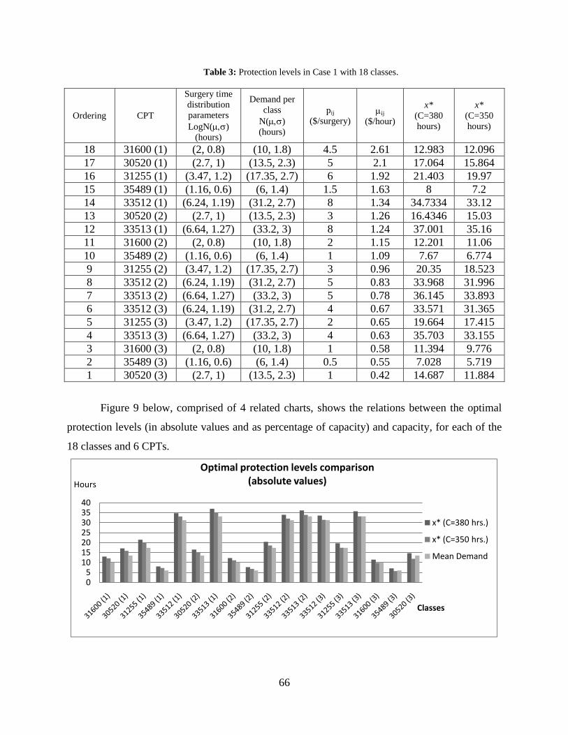
66
Table 3: Protection levels in Case 1 with 18 classes.
Ordering CPT
Surgery time
distribution
parameters
LogN()
(hours)
Demand per
class
N()
(hours)
pij
($/surgery) ij
($/hour)
x*
(C=380
hours)
x*
(C=350
hours)
18 31600 (1) (2, 0.8) (10, 1.8) 4.5 2.61 12.983 12.096
17 30520 (1) (2.7, 1) (13.5, 2.3) 5 2.1 17.064 15.864
16 31255 (1) (3.47, 1.2) (17.35, 2.7) 6 1.92 21.403 19.97
15 35489 (1) (1.16, 0.6) (6, 1.4) 1.5 1.63 8 7.2
14 33512 (1) (6.24, 1.19) (31.2, 2.7) 8 1.34 34.7334 33.12
13 30520 (2) (2.7, 1) (13.5, 2.3) 3 1.26 16.4346 15.03
12 33513 (1) (6.64, 1.27) (33.2, 3) 8 1.24 37.001 35.16
11 31600 (2) (2, 0.8) (10, 1.8) 2 1.15 12.201 11.06
10 35489 (2) (1.16, 0.6) (6, 1.4) 1 1.09 7.67 6.774
9 31255 (2) (3.47, 1.2) (17.35, 2.7) 3 0.96 20.35 18.523
8 33512 (2) (6.24, 1.19) (31.2, 2.7) 5 0.83 33.968 31.996
7 33513 (2) (6.64, 1.27) (33.2, 3) 5 0.78 36.145 33.893
6 33512 (3) (6.24, 1.19) (31.2, 2.7) 4 0.67 33.571 31.365
5 31255 (3) (3.47, 1.2) (17.35, 2.7) 2 0.65 19.664 17.415
4 33513 (3) (6.64, 1.27) (33.2, 3) 4 0.63 35.703 33.155
3 31600 (3) (2, 0.8) (10, 1.8) 1 0.58 11.394 9.776
2 35489 (3) (1.16, 0.6) (6, 1.4) 0.5 0.55 7.028 5.719
1 30520 (3) (2.7, 1) (13.5, 2.3) 1 0.42 14.687 11.884
Figure 9 below, comprised of 4 related charts, shows the relations between the optimal
protection levels (in absolute values and as percentage of capacity) and capacity, for each of the
18 classes and 6 CPTs.
05
10152025303540
Hours
Classes
Optimal protection levels comparison (absolute values)
x* (C=380 hrs.)
x* (C=350 hrs.)
Mean Demand
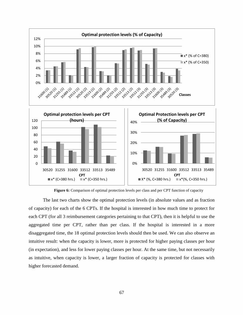
67
Figure 6: Comparison of optimal protection levels per class and per CPT function of capacity
The last two charts show the optimal protection levels (in absolute values and as fraction
of capacity) for each of the 6 CPTs. If the hospital is interested in how much time to protect for
each CPT (for all 3 reimbursement categories pertaining to that CPT), then it is helpful to use the
aggregated time per CPT, rather than per class. If the hospital is interested in a more
disaggregated time, the 18 optimal protection levels should then be used. We can also observe an
intuitive result: when the capacity is lower, more is protected for higher paying classes per hour
(in expectation), and less for lower paying classes per hour. At the same time, but not necessarily
as intuitive, when capacity is lower, a larger fraction of capacity is protected for classes with
higher forecasted demand.
0%
2%
4%
6%
8%
10%
12%
Classes
Optimal protection levels (% of Capacity)
x* (% of C=380)
x* (% of C=350)
0
20
40
60
80
100
120
30520 31255 31600 33512 33513 35489
CPT
Optimal protection levels per CPT (hours)
x* (C=380 hrs.) x* (C=350 hrs.)
0%
10%
20%
30%
40%
30520 31255 31600 33512 33513 35489
CPT
Optimal Protection levels per CPT (% of Capacity)
X* (%, C=380 hrs.) x*(%, C=350 hrs.)
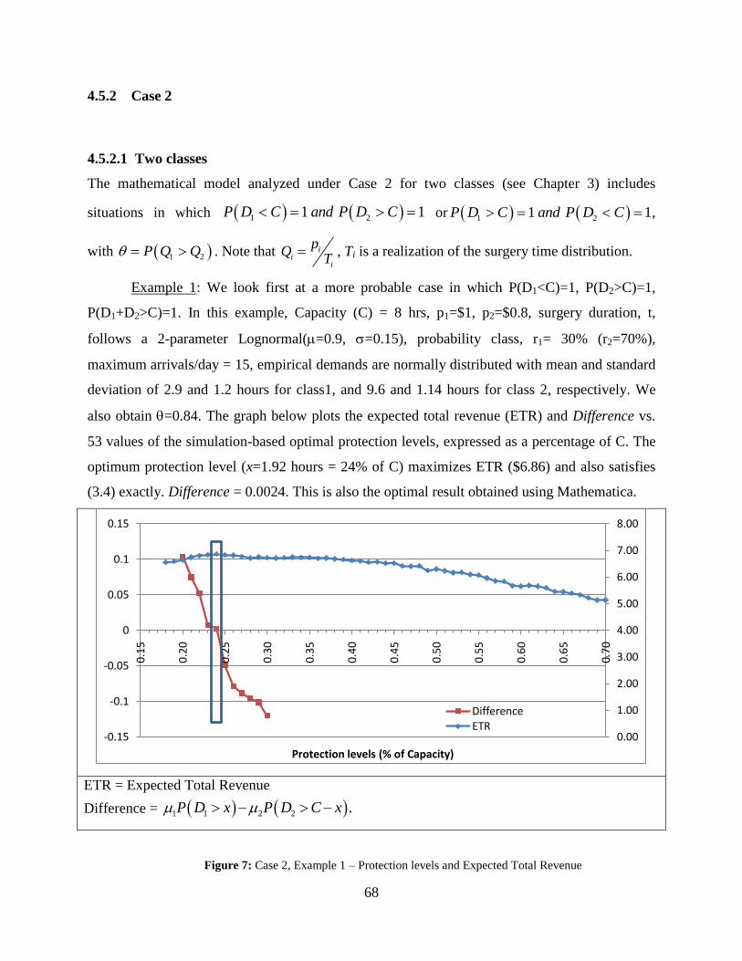
68
4.5.2 Case 2
4.5.2.1 Two classes
The mathematical model analyzed under Case 2 for two classes (see Chapter 3) includes
situations in which 1 21 1P D C and P D C or 1 21 1P D C and P D C ,
with 1 2P Q Q . Note that ii
i
pQ
T , Ti is a realization of the surgery time distribution.
Example 1: We look first at a more probable case in which P(D1<C)=1, P(D2>C)=1,
P(D1+D2>C)=1. In this example, Capacity (C) = 8 hrs, p1=$1, p2=$0.8, surgery duration, t,
follows a 2-parameter Lognormal(=0.9, =0.15), probability class, r1= 30% (r2=70%),
maximum arrivals/day = 15, empirical demands are normally distributed with mean and standard
deviation of 2.9 and 1.2 hours for class1, and 9.6 and 1.14 hours for class 2, respectively. We
also obtain =0.84. The graph below plots the expected total revenue (ETR) and Difference vs.
53 values of the simulation-based optimal protection levels, expressed as a percentage of C. The
optimum protection level (x=1.92 hours = 24% of C) maximizes ETR ($6.86) and also satisfies
(3.4) exactly. Difference = 0.0024. This is also the optimal result obtained using Mathematica.
ETR = Expected Total Revenue
Difference = 1 1 2 2 . P D x P D C x
Figure 7: Case 2, Example 1 – Protection levels and Expected Total Revenue
0.00
1.00
2.00
3.00
4.00
5.00
6.00
7.00
8.00
-0.15
-0.1
-0.05
0
0.05
0.1
0.15
0.1
5
0.2
0
0.2
5
0.3
0
0.3
5
0.4
0
0.4
5
0.5
0
0.5
5
0.6
0
0.6
5
0.7
0
Protection levels (% of Capacity)
DifferenceETR
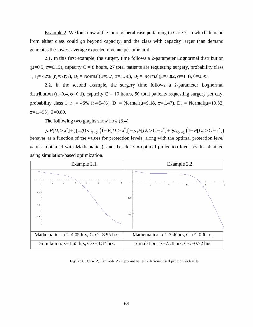
69
Example 2: We look now at the more general case pertaining to Case 2, in which demand
from either class could go beyond capacity, and the class with capacity larger than demand
generates the lowest average expected revenue per time unit.
2.1. In this first example, the surgery time follows a 2-parameter Lognormal distribution
(=0.5, =0.15), capacity C = 8 hours, 27 total patients are requesting surgery, probability class
1, r1= 42% (r2=58%), D1 = Normal(=5.7, =1.36), D2 = Normal(=7.82, =1.4), =0.95.
2.2. In the second example, the surgery time follows a 2-parameter Lognormal
distribution (=0.4,=0.1), capacity C = 10 hours, 50 total patients requesting surgery per day,
probability class 1, r1 = 46% (r2=54%), D1 = Normal(=9.18, =1.47), D2 = Normal(=10.82,
=1.495), =0.89.
The following two graphs show how (3.4)
1 2 1 2
* * * *
1 1 1| 1 2 2 2| 2[ ] 1 [ ] [ ] 1 [ ]1 Q Q Q QP D x P D x P D C x P D C x
behaves as a function of the values for protection levels, along with the optimal protection level
values (obtained with Mathematica), and the close-to-optimal protection level results obtained
using simulation-based optimization.
Example 2.1. Example 2.2.
Mathematica: x*=4.05 hrs, C-x*=3.95 hrs. Mathematica: x*=7.40hrs, C-x*=0.6 hrs.
Simulation: x=3.63 hrs, C-x=4.37 hrs. Simulation: x=7.28 hrs, C-x=0.72 hrs.
Figure 8: Case 2, Example 2 - Optimal vs. simulation-based protection levels
2 3 4 5 6 7 8
1.5
1.0
0.5
2 4 6 8 10
1.0
0.5

70
There are several reasons as to why there are small differences between the protection
level results obtained with Mathematica vs. simulation. While randomness clearly plays a large
role when simulating data, an equally (if not more) likely reason is that in the simulation model
the protection levels may not be entirely used up during every booking window. This happens
when the generated time for an additional patient would not fit within the remaining time for that
patient‟s class protection level and hence he/she is not included in the set of patients scheduled
for that particular period. This leads to some idle time, for all classes, for which no revenue is
incurred by the surgical unit. In the two cases above, the average idle time was about 0.3 hours.
At the same time, the mathematical model assumes that the surgery time is small enough
when compared to capacity, so that one could exactly fit an integer number of surgeries during
the scheduling horizon, and theoretically incur revenue across all allocated time. While this is a
reasonable assumption to make when some overtime is allowed, it is not guaranteed to happen in
practice when the capacity is strict. While these idle and overtime situations are not included in
the theoretical or in the simulation model, they are frequently encountered in practice. Usually,
the scheduler places patients into the schedule only based on average surgery duration, and idle
and overtime are incurred because the actual surgery duration goes below/beyond the estimated
time. When surgical times are modeled using the lognormal distribution, more than 50% of the
time the actual surgery lasts longer than the assumed mean duration.
Conjecture 4: When 0,it
C then the relative value
| * |0
*
x x
x
and idle time 0,
where x is the simulation-based optimization protection level, x* is the theoretical optimal
protection level, and it is the mean surgical duration.
In the two examples above, the ratio it
C drops from 6.25% for Example 2.1. to 4% in
Example 2.2; the ratio | * |
*
x x
x
drops from 10.3% to 1.6%. When capacity is increased from 10
to 30 hours in Example 2.2, the ratio 1.67%it
C and the ratio
| * |
*
x x
x
drops to less than 0.1%.
Another observation that needs to be made is that it is possible that *x C . A protection
level equal to capacity means that there is no time to be protected for the second class during that
planning horizon.

71
4.5.2.2 Three classes
We now look briefly into Case 2 for n = 3 classes of patients requesting same surgery. As a first
step, it is necessary to assess the six (n! = 3!) s, that are used to numerically compute the two
protection levels, *
1x and *
2x . Since *
2x includes *
1x , the time allocated to the class that on average
brings the smallest revenue per unit of time is computed as *
2max{0, }C x
The following example assumes that surgery time, t, follows a 2-parameter Lognormal
(=0.5, =0.15), probabilities for class 1, 2, 3 are 25%, 35%, and 40% respectively. p1/p2=1/0.9
= 1.11, and p2/p3 = 0.125. D1 = Normal(=5.6, =1.45), D2 = Normal(=7.82, =1.648), D3 =
Normal(=9, =1.7), capacity C = 12 hours. The theoretical optimal protection levels for which
equation (3.6) holds are found numerically with Mathematica to be: *
1x = 4.53 hours, *
2x = 10.6
hours. This means that class 1 gets 4.53 hours, class 2 gets 10.6-4.53 = 6.07 hours, and the
remaining 12-10.6 = 1.4 hours being allocated for class 3 patients. Very close values for the
protection levels were found using simulation-based optimization.
The 3D graph below illustrates the uniqueness of the optimal result above using (3.6).
(3.6) involves solving a system of two equations with two unknowns (x1 and x2) and is of form: a
= b and b = c, with:
2 3 1 3 2 1
1 3 2 3 1 2
* *
1 1 1 231 1| 321 1| 1 1
* * * *
2 2 2 1 132 2| 312 2| 2 2 1
[ ] 1 [ ]
[ ] 1 [ ]
Q Q Q Q Q Q
Q Q Q Q Q Q
a P D x P D x
b P D x x P D x x
1 2 3 2 1 3
* *
3 3 2 123 3| 213 3| 3 2[ ] 1 [ ]Q Q Q Q Q Qc P D C x P D C x
The graph below plots the surfaces represented by a, b and c defined above. Their only
intersection point is of coordinates ( *
1x , *
2x ), i.e. (4.53, 10.6) hours.

72
Figure 9: 3D Plot of (6) for Case 2 with 3 classes
4.5.2.3 Multiple classes
In the case of 3n customer classes, could happen that *
n ix C , which means that during the
planning horizon under consideration, no patients pertaining to last i classes are scheduled for the
booking window under consideration. If capacity cannot be expanded, either by opening another
operating room or allowing for overtime, then only patients in classes 1,...,n i will be
scheduled, with patients in other classes being postponed until a later date.
As we move into more complex situations, with 2j number of surgeries and 2i
reimbursement categories, we deal with a higher number of total classes (n=i*j), which requires
the computation of n! values (under Case 2 assumptions), to be used to numerically compute
the optimal protection levels.
Example 1: We consider that patients requesting one of two surgeries have one of the 2
possible insurance categories. Surgery1 (CPT 36489) follows a 2-parameter Lognormal(=1.15,
=0.6) and Surgery2 (CPT 52000) follows a 2-parameter Lognormal(=0.68, =0.32). The
surgical unit is making scheduling decisions for periods of C = 40 hours. We computed the 4! =
24 values using simulation.
Let j iS C be the label for a category for a patient having insurance category i and
requesting surgery j. Based on the 4 ij ‟s, the ordering across the 4 classes is: S1C1, S2C1, S1C2,

73
S2C2. The information on the surgical times, prices and optimal protection levels is presented in
Table 4 below. The optimal protection levels are obtained using (3.7).
Table 4: Protection levels in Case 2 with 4 classes.
Ordering Name pij ($/surgery) ij ($/hour) Demand (hrs/week)
N(,)
Optimal x (hours/class)
4 S1C1 2 2.20 9.62, 2.4 11.3
3 S2C1 1 1.80 7.57, 2.3 9.1
2 S1C2 1.5 1.65 9.34, 2.65 11.16
1 S2C2 0.8 1.44 8.18, 1.56 8.44
Example 2: We now assume that patients could have any of 3 possible insurance
categories, requesting one of the two surgeries mentioned in the previous example. This
generates 6 total classes of patients, which requires the computation of the 6! = 720 q values
needed to numerically find the optimal protection levels using (3.7). We obtained the 720 thetas
using simulation. With a capacity C = 50 hours, the surgical department would maximize
expected revenue if it would reserve for each class the hours presented in Table 5 below (x* =
optimal x).
Table 5: Protection levels in Case 2 with 6 classes.
Ordering Name pij ($/SjCi) ij ($/hour) Demand (hrs/week)
N(,)
x*
(hours/class)
6 S1C1 2 2.20 9.62, 2.4 11
5 S2C1 1 1.80 7.57, 2.3 8.56
4 S1C2 1.5 1.65 9.34, 2.65 10.3
3 S2C2 0.8 1.44 8.18, 1.56 8.55
2 S1C3 1 1.11 5.38, 2.17 5.6
1 S2C3 0.6 1.07 5.9, 2.1 6
4.5.3 Conclusions and revenue results
In the previous examples we have described the inputs and the results (optimal protection levels)
for several examples, for both cases analyzed in Chapter 3. The theoretical models apply

74
similarly regardless of how many surgeries and reimbursement categories are considered and
deemed necessary. Theoretically, based on the mathematical proofs in Chapter 3, the
implementation of these optimal protection levels would lead to the maximum expected revenue.
We were not able to make revenue comparisons between the optimal ones versus the ones
obtained in practice, because the information on the actual revenues obtained when these
surgeries were performed, was not available. We do have results on the revenue gap between the
optimal revenue and the one obtained under the first come first served (FCFS) scheduling policy.
Over the examples we analyzed, the optimal expected revenue was, on average, 1.9% larger than
the one obtained if a FCFS scheduling policy were to be used. This revenue gap value is similar
to the ones reported in the revenue management practices
The mathematical model assumes that revenue is incurred for the entirety of the
protection levels; this may not be the case in practice, because there is significant uncertainty in
the duration of activities related to the surgical procedure (Denton, Rahman et al. 2006). Due to
the customized nature of the technical procedures, idle time, over- and under-utilization may
occur. To minimize it, the hospital further needs to find an efficient way to break down the
protection levels across days and/or surgical suites, while considering and balancing the over-
and under-utilization times and costs.
4.6 PROBLEM COMPLEXITY
With an increased number of classes, our problem suffers from the curse of dimensionality, and
computing the necessary values could pose some computational issues in practice. Our
problem reduces to a stochastic knapsack problem with random item (surgery) sizes, known
exactly only after the selection decision has been made, and known item values at the time of the
decision. Random surgery realizations are to be known only after the selections are made. The
general knapsack problem is known to be NP-hard (Garey and Johnson 1979). Therefore the
running time is O(2n), where n = number of total classes. Several algorithms for handling the
stochastic knapsack problem with random weights are summarized by Kellerer et. al. (2004).

75
4.7 HEURISTIC SOLUTION
When the surgical department has to schedule patients in need for one of the multiple surgeries
handled by the surgical team, and when these patients have different levels of medical insurance,
it may become too time consuming for the scheduling personnel to employ the mathematical
model in order to optimally decide on the time to allocate for each class of patients, and,
consequently, on how many patients from each class to accept over the booking horizon. The
complexity is due to the size of the problem which increases faster than exponential in the
number of classes. To speed up the process, we propose a heuristic which can be considered an
extension/modification of the well known EMSRb heuristic (Belobaba 1989). We name our
heuristic Expected Marginal Capacity Revenue for Operating Rooms (EMCR-OR).
Given N surgeries (CPTs) and M reimbursement categories, a patient‟s class will be
determined based on the type of surgery requested (1,…,j,…N) and the reimbursement category
(1,…,i,…M). We define by k the class of the request (the combination of patient‟s insurance
type and surgery requested), with 1,...,k K and K M N . The revenues per surgeries follow
the relation1 2 1... ...k k Kp p p p p , while the ranking within the k classes of patients is
based on the order statistics of k
j
pt
, which is based on the random realization of surgical times.
To be noted that while the price per surgery, kp , is fixed, because the actual surgical time
follows some probability distribution, the revenue/unit of time,
k
j
pt
, is also a random variable;
the mean of the distribution of k
j
pt
is the expected revenue per unit of time collected when
surgery type j is performed for a category i patient. The question then becomes how many time
units (minutes, 5-minute periods, etc) should be protected, in a nested fashion, for class j and
higher, or in a partitioned fashion, for each individual class, in order to maximize expected
revenue.
In what follows, we present how our heuristic works. The result takes the form of close-
to-optimal protection levels (time allocations) that would give the scheduler a very good insight
into how many time units to protect for each insurance class within a surgical type. This
information becomes the basis for deciding, during each day or planning period, the number of
76
ORs to open and the number of surgeries to be performed for each customer type requesting a
certain surgery.
In practice, the heuristic approaches are preferred to the optimal calculations due to the
intuition behind them, faster computation time, and only about ½% revenue gap (Talluri and Van
Ryzin 2004). We discussed in Chapter 2 about various heuristic used in practice. In what follows
we present our heuristic (EMCR-OR), which is an extension to the EMSRb (expected marginal
seat revenue, version b) heuristic, adapted to take into account the variability in service time, and
consequently in the revenues per unit of time. By using simulation to run our heuristic, we obtain
a distribution of protection levels (for each class of patients), the mean of which is reported as
the close-to-optimal protection level for that class. To find the distributions of protection levels
we proceed as follows:
Step 1: Define the unit of resource, in this case the time unit (seconds, minutes or hours).
Step 2: Identify the N surgeries (CPTs) that compete for the C units of time available
(budgeted) in the OR (ORs), for the scheduling horizon (day, week, etc)
Step 3: Estimate the coverage percentage for the types of reimbursement (insurance
coverage) considered. For each surgery involved identify the price per surgery that each type of
insurance would cover. If we assume only three possible types of insurance/coverage for
example, and if we further consider that a full-coverage type of insurance covers 1% c of the cost
of surgery, a partial coverage covers 2 % c , and low-partial coverage covers
3% c , then for each
surgery j with price jp we will obtain 3 classes of prices:
1 2 3j j jp c p c p c , with j i kp c p . If
more insurance classes are considered, then for each CPT we will obtain that many price classes.
Step 4: Obtain the surgery price per unit of time, k
j
pt
, by dividing, for each CPT, each
of the relevant prices obtained above by random variables drawn from the surgery‟s specific
duration distribution. Obtain the mean for each k
j
pt
, k , for the purpose of ranking these K
classes of patients.
Step 5: Sort these newly obtained mean prices in descending order. Let the order statistics
be (1) ( ) ( )... ...k K . For example, with 3 surgeries and 3 classes, there will be a total of 9
77
resulting classes of patients, with an expected revenue k
assigned to each, and
1 2 ... ...k K , intertwined with respect to the ranking within a CPT class.
Step 6: Determine the demand distribution kD for each of the k = 1,…,K classes. Here we
need information about the expected demand for a particular type of surgery during that period
of time, and about the probability of a patient‟s request for surgery type j to belong to insurance
category i.
Step 7: Define the aggregated future demand for classes , 1,...,1k k by 1
K
k k
k
A D
Step 8: Compute the weighted average revenue from classes 1,…,k 1
1
[ ]
[ ]
K
k k
kk K
k
k
E D
E D
Step 9: The nested protection level for class k and higher,kx , is chosen (using
Littlewood‟s rule, when two classes are present) so that:
1( ) kk k
k
P A x
Step 10: Obtain1 2 1( , ,..., ,..., )j KX x x x x , the vector of nested protection levels.
Kx could
then be obtained as -1max{0, - }.KC x
Step 11: Disaggregate the protection levels, by assigning the protection levels per
individual surgeries, so that 1k kx x time units are allocated to class k.
Step 12: Using simulation, obtain the distributions for each disaggregate protection level
and compute the mean. These means become the-close-to-optimal protection levels reported for
each class.
If the surgical department is interested in pooling the total available time for all N types
of surgeries provided, and then compute protection levels for all N*M possible surgery-demand
class combination, then it needs to generate N*M-1 protection levels. If it is interested in
deciding how much OR time to allocate for one reimbursement class patients within one
particular surgery, then it needs to compute only M-1 protection levels for that procedure.

78
4.7.1 Heuristic implementation and solution
We present examples to show the algorithm‟s implementation and performance, and compare the
heuristic results versus the optimal ones.
First, consider the two examples presented in section 4.5.2.3 (Surgery 1: CPT 36489,
Surgery 2: CPT 52000). Applying the heuristic, we get the following values for the protection
levels ( x ), shown in Table 6 below along with the optimal ones ( *x ).
Table 6: Protection levels comparison (x and x*) for 4 and 6 classes
2 Surgeries, 2 Classes (C=40 hrs.) 2 Surgeries, 3 Classes (C=50 hrs.)
Name x* (hrs) x (hrs) x*-x |x*-x|/x* Name x* (hrs) x (hrs) x*-x |x*-x|/x*
S1C1 11.3 10.1 1.2 10.6% S1C1 11 9.5 1.5 13.63%
S2C1 9.1 8.73 0.37 4% S2C1 8.56 7.8 0.76 8.87%
S1C2 11.16 10.77 0.39 3.5% S1C2 10.3 9.68 0.62 6.02%
S2C2 8.44 10.4 -1.96 23.23% S2C2 8.55 9.06 -0.51 5.96%
S1C3 5.6 6.67 -1.07 19.1%
S2C3 6 7.23 -1.23 20.5%
Two surgeries, two reimbursement categories Two surgeries, three reimbursement categories
Figure 10: Protection levels comparison (x and x*) for 4 and 6 classes
0
5
10
15
S1C1 S2C1 S1C2 S2C2
Patient Classes
Protection levels comparison
x* (hrs)
x (hrs)
0
5
10
15
S1C1 S2C1 S1C2 S2C2 S1C3 S2C3
Patient Classes
Protection levels comparison
x* (hrs)
x (hrs)
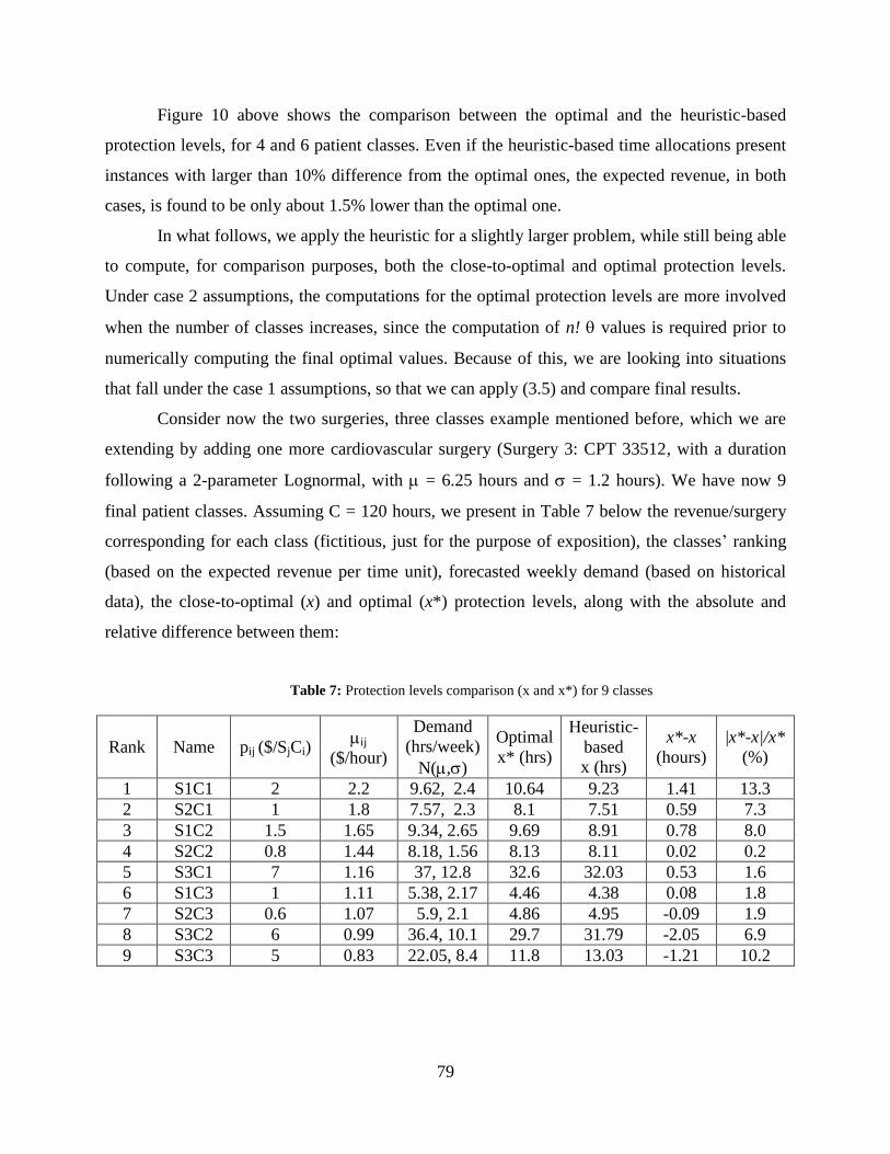
79
Figure 10 above shows the comparison between the optimal and the heuristic-based
protection levels, for 4 and 6 patient classes. Even if the heuristic-based time allocations present
instances with larger than 10% difference from the optimal ones, the expected revenue, in both
cases, is found to be only about 1.5% lower than the optimal one.
In what follows, we apply the heuristic for a slightly larger problem, while still being able
to compute, for comparison purposes, both the close-to-optimal and optimal protection levels.
Under case 2 assumptions, the computations for the optimal protection levels are more involved
when the number of classes increases, since the computation of n! values is required prior to
numerically computing the final optimal values. Because of this, we are looking into situations
that fall under the case 1 assumptions, so that we can apply (3.5) and compare final results.
Consider now the two surgeries, three classes example mentioned before, which we are
extending by adding one more cardiovascular surgery (Surgery 3: CPT 33512, with a duration
following a 2-parameter Lognormal, with = 6.25 hours and = 1.2 hours). We have now 9
final patient classes. Assuming C = 120 hours, we present in Table 7 below the revenue/surgery
corresponding for each class (fictitious, just for the purpose of exposition), the classes‟ ranking
(based on the expected revenue per time unit), forecasted weekly demand (based on historical
data), the close-to-optimal (x) and optimal (x*) protection levels, along with the absolute and
relative difference between them:
Table 7: Protection levels comparison (x and x*) for 9 classes
Rank Name pij ($/SjCi) ij
($/hour)
Demand
(hrs/week)
N(,)
Optimal
x* (hrs)
Heuristic-
based
x (hrs)
x*-x
(hours)
|x*-x|/x*
(%)
1 S1C1 2 2.2 9.62, 2.4 10.64 9.23 1.41 13.3
2 S2C1 1 1.8 7.57, 2.3 8.1 7.51 0.59 7.3
3 S1C2 1.5 1.65 9.34, 2.65 9.69 8.91 0.78 8.0
4 S2C2 0.8 1.44 8.18, 1.56 8.13 8.11 0.02 0.2
5 S3C1 7 1.16 37, 12.8 32.6 32.03 0.53 1.6
6 S1C3 1 1.11 5.38, 2.17 4.46 4.38 0.08 1.8
7 S2C3 0.6 1.07 5.9, 2.1 4.86 4.95 -0.09 1.9
8 S3C2 6 0.99 36.4, 10.1 29.7 31.79 -2.05 6.9
9 S3C3 5 0.83 22.05, 8.4 11.8 13.03 -1.21 10.2

80
Figure 11: Protection levels comparison for 9 classes
Figure 11 above shows the optimal and heuristic-based protection levels The mean
absolute percentage error (|x*-x|/x*) is about 5.7%, while the percentage error ((x*-x)/x*) is
about 1.5%. The revenue optimality gap, computed using simulation (10,000 iterations) with
random patient arrivals, is only 0.7%. From the examples above we could also notice that the
heuristic underestimates the protection levels for the first classes (that is, * 0x x ), and it
overestimates the protection levels for the last classes ( * 0x x ).
The heuristic is attractive in practice, with just slight loss in expected revenue, but with
the advantage of less computational time. Further calculations need to be performed to obtain
more accurate information on the performance of this proposed heuristic in practice, from both
the revenue and computational time perspectives.
4.7.2 Heuristic application: an extension
Overtime is necessary in the situations where a surgery goes beyond the end of the budgeted OR
time for that day, since we assume that no surgery will continue on the next day. Subsequently,
once a decision is made to start a surgery, in the event that it goes beyond the budgeted time, it
will incur overtime cost, which usually is higher than the cost of regular time.
Strum and Vargas (1997) developed a minimal cost analysis (MCA) approach to decide
on the time allocations across subspecialties in order to minimize under and overutilization costs,
0
5
10
15
20
25
30
35
S1C1 S2C1 S1C2 S2C2 S3C1 S1C3 S2C3 S3C2 S3C3
Hours
Patient Classes
x*
x

81
based on the ratio of overtime to regular time cost per unit of time. When overtime is allowed
and unavoidable, we can incorporate this idea when allowing for overtime in our situation. After
obtaining the distribution of protection levels for each category, instead of reporting the mean,
we can decide on a threshold (cut-off) value, other than the mean, that would represent the
minimum time the surgical department should allocate for that class, in an attempt to increase
revenue and decrease overtime costs. For example, if the ratio between overtime and regular
costs per time unit is 2, then we can use the 66.7th
percentile of each distribution as being the
number of units of time to be assigned for that patient category.
To illustrate this extension, we start by presenting the graphs below, as part of Figure 12,
that show these protection levels distributions for the nine classes in the previous example, along
with the mean and the 66.7th
percentile values. The values for the 66.7th
percentiles could be used
when overtime is allowed.
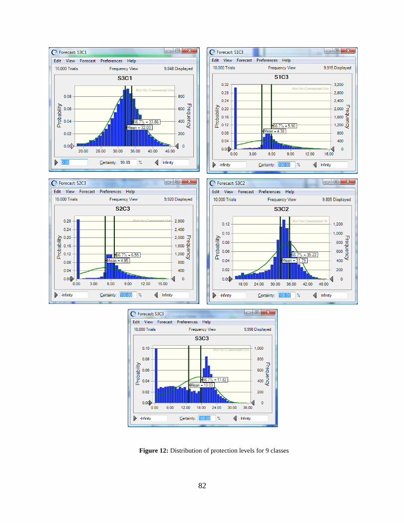
82
Figure 12: Distribution of protection levels for 9 classes

83
We further used simulation to compute the increase in expected revenue (versus the
optimal one) when using, as protection levels, the 66.7th
percentile of the protection level
distributions, rather than the mean of those distributions. The results obtained show that the new
protection levels would result in an 11.5% increase in expected revenue, which comes with an
average capacity usage of about 123 hours; this represents an average overtime of 3 hours, 2.5%
of the initial capacity of 120 hours.
While overtime is not desirable, it may become necessary in situations where unexpected
complications arise, or when longer surgeries are scheduled during a day. While the former
situation cannot be predicted, the latter should take into account the probability of going over the
allocated time, due to the potential costs involved. The models presented here should be coupled
with rigorous forecasting and prediction methods, helping the decision maker determine and
implement more accurate protection levels.

84
5.0 CONCLUSIONS AND FUTURE RESEARCH
5.1 SUMMARY
The implementation of Revenue Management techniques proved to be very successful in many
business areas, from airlines to TV advertising, from cruise cabin management to car rentals. A
common assumption in many of these previously analyzed situations is that when a customer‟s
request is accepted, the request will use up only the amount of resource that it was approved for.
In services, this is not the case all the time. This work focuses on analyzing the allocation
(reservation) of fixed capacity across multiple customer classes, in the case where the accepted
customers‟ requests use up a variable amount of the resource under consideration. We look
especially at situations faced by a surgical unit that is in the process of planning and scheduling
elective surgeries for a certain future period.
We analyze a very realistic situation in which the actual service duration is known with
certainty only after the procedure is performed, but scheduling customers‟ requests should be
performed days before this happens. At the same time, customers arrive in a random order,
which adds another level to difficulty to the classical revenue management problem. Our
mathematical model provides the optimal time allocations to various customer classes in the
form of protection levels, which dictate the maximum amount of resource (time) that should be
reserved for a particular type of service. In chapter 4 we focus on applying the model in
scheduling elective surgeries, which do not present medical urgency.
It is assumed that customers can be segmented based on their need for a specific surgery,
and on reimbursement category, function of their health insurance coverage. The latter criterion
could be dropped in the case of cosmetic surgeries, for example, which are not usually covered
by health insurance. The usage of optimal protection levels would determine which patients to be
accepted and which to be postponed, resulting in maximizing the expected revenue incurred by
85
the surgical unit. Patients will be accepted up to the protection level for that class, and the
postponed ones will be scheduled for a later date at which the protection level for that class and
for that time period will accommodate that patient.
This study is intended to offer a solid starting point for the analysis of time allocation and
scheduling in a complex service environment characterized by uncertain service duration and
random customer arrivals. In particular, our examples are in the healthcare arena, but the
mathematical model has applicability in many other service sectors, and even manufacturing.
While there are many tradeoffs and criteria that decision makers need to consider when
budgeting time and booking patients‟ request for service, the model presented in this thesis can
be used as a decision and planning tool to improve the operational decision making when
delivering surgical services. Its implementation would have a direct impact on increasing
revenue and quality of healthcare. We recognize that the model can be extended or modified to
account for other various situations encountered in practice, additions which would make the
problem we present here of an even greater importance.
As an extension, the decision maker can incorporate a deadline, class related, until which
all requests older than a predefined value should be scheduled without incurring a penalty.
Penalties could take different forms, both monetary and non-monetary, from deterioration in the
health condition of a patient, to some monetary penalty imposed by the hospital for postponed
surgical requests. At the same time, a postponed surgery means postponed revenue for the
hospital. A postponed surgery could transform in a lost surgery if the patient switches providers
due to the long wait. “Medical tourism” is now a viable alternative to the traditional inpatient or
outpatient elective surgeries locations. The conclusion is that an efficient time allocation across
classes of patient in the form of protection levels is of crucial importance for improving the
revenue of the health care unit. Incremental revenue could be used for capacity expansion, so
that, when coupled with adequate personnel, could help the surgical unit accommodate more
surgeries in the long run, thus improving the quality of care.

86
5.2 MODEL EXTENSIONS
The optimal protection levels calculations we present in this paper are derived on the realistic
assumption that any service duration is a random variable. We showed how the model is
different than the traditional revenue management models which assumed constant resource
usage per request. We compute optimal results when none of the classes‟ demand is expected to
be larger than the available capacity during the scheduling horizon (but together would); we also
show how the model changes when one of the classes‟ demand it is expected to be larger than
capacity. In this latter situation, the computations of the n! thetas (the probability of the orderings
between the expected revenues per time unit) increases the size and complexity of the problem.
For this instance we propose a heuristic approach which gives very good results in practice, and
can accommodate a large number of classes.
Overtime sometimes is a necessary evil when it comes to providing service, but it usually
comes at a significant cost. In healthcare, overtime could arise due to overbooking or just
because scheduled surgeries for a day go beyond the regular time due to the inherent variability
in procedure times. Under- and over-utilization, as described by Strum et.al. (1997), can be
reduced if a better time allocation is used, accounting for the services probability distribution.
While the heuristic extension we presented previously includes the possibility of overtime, the
optimization model does not allow for overtime, nor does it incorporate overtime situations. This
constitutes an opportunity for continued research in this area. This links into the decision of
whether or not to accept one more patient for the scheduling period under consideration.
5.2.1 Deciding the number of patients to accept
The mathematical model provides the scheduler with the optimal maximum time to reserve for
each patient class (given by the optimal protection levels), but does not give the answer for the
optimal number of patients to accept during that planning horizon. The simulation models used
to compute the expected revenues based on the optimal protection levels include in the schedule
only patients whose a-priori simulated service times would not go beyond the remaining time for
each class‟ protection level. A policy that is used in practice to decide whether to accept a new
87
patient is to compare the average procedure duration with the remaining time, and if the
remaining time accommodates this average, then the patient is included in the schedule. In this
situation, overtime is possible. As most surgical procedures follow a 2 or 3 parameter lognormal
distribution, it is unlikely that the mean surgical duration is the best general criterion for adding
another patient into the schedule. The analysis should also include the tradeoffs between the cost
of idle time and under-utilization and the cost of overtime or over-utilization, along with a
thorough estimation of procedure‟s duration. The latter factor is critical in computing the average
revenue per unit of time, which is part of optimally computing the protection levels.
5.2.2 Forecasting demand and deciding on the length of the booking period
The health care unit needs to correctly forecast demand, per type of surgery and per
reimbursement category. Historical data are a starting point, which should be updated with recent
changes in population structure, fee-for-service structure, and national and regional surgery
prices. The ability to accurately track and forecast demand links into the decision on how long
the scheduling horizon should be. The scheduling period, during which some of the previous
requests would be scheduled, influences the capacity available, which can be modified by the
decision of how many operating rooms to use for a day or for a type of procedure.
In practice, reservation requests from different customer classes do not arrive in a
predetermined fashion (i.e., in a decreasing or increasing order of the expected revenue per unit
of time, or sequentially, per type of surgery), but rather in a concurrent fashion. Our
mathematical model recognizes this fact, and the optimal results apply for the situation of
random customer arrivals. But the ability of the decision making unit to successfully compute
and implement these results also lays on the determination of the appropriate length of the
planning period.
Longer booking periods translate in a larger capacity available, which means that there is
a low probability than any of the customer classes‟ demand for that period of time would go
beyond capacity. In this case, the surgical unit could implement the results given by Case 1 to
compute the optimal protection levels. The downside of using longer planning intervals, though,

88
is that there is no fast reaction to changes in demand patterns, if they happen. This is equivalent
to a static booking policy, where the demand is updated only at rarely during the booking period.
Shorter scheduling intervals translate in a lower capacity available during that period,
which increases the chance of any of the classes‟ demand to go beyond capacity. Our assumption
in this case is that the class that on average generates the lower revenue per time unit is the one
whose demand goes beyond capacity. In this situation, computing the n! thetas may increase the
time to get the optimal protection levels. But shorter scheduling periods come with the advantage
of demand distribution for each class being reevaluated at the beginning of each planning period,
thus incorporating the potential demand changes that occurred in the meantime. At the same
time, the shorter scheduling periods have the advantage of automatically incorporating
cancellations and no show, and managing them in an urgent fashion is critical for an efficient
appointment system. This is similar to the dynamic booking model, where the demand updates
are frequent, to better capture demand changes.
5.2.3 Deciding how many operating rooms to open
Operating rooms are a main factor for a hospital‟s operating cost and revenues. The number of
available surgical suites influences how well the hospital can manage the demand for elective
surgeries in an uncertain environment. A surgical unit manages a certain number of ORs that
could be used for specific subspecialties only, or could be used interchangeably. Increasing
available surgical capacity over the scheduling horizon can be done either by opening more ORs,
or by opening the same number of ORs but for longer hours each day. The decision is influenced
by the flexibility of the surgical personnel and the costs of overtime versus opening another OR.
This area is rich in relevant work that can help with this decision.

89
5.3 FUTURE STUDIES
Hospitals should be in a continuous search for more efficient and timely utilization of their
resources (time, ORs, personnel) to better respond to patients‟ demand for service. We offer here
such a suggestion that would help hospitals make better decisions at the strategic and operational
level. Besides answering the questions on how much time to optimally protect for each class of
patients, our results offer insights about how many ORs to allocate per subspecialty, what would
be an adequate advance booking period, and what would be the surgeries that need to be
performed in specialty ORs.
The problem is complex and our model tries to incorporate some revenue management
techniques that, despite their proven results in airline and hotel management, are still not very
widespread in the healthcare sector. We presented the particularities of these techniques when
applied in healthcare and we believe that continued research in this direction will provide
hospital managers and administrators with adequate decision making tools.
5.3.1 Dynamic programming and the time value of money
It is necessary for the hospital to recognize that the timing of incurring the revenue does matter.
Even when the same set of surgeries is performed over a period of time, their sequencing is
going to influence the net value of the total revenue incurred for that period. If the booking
period is broken down into stages (days, for example), the problem of finding the optimal
protection levels at these intervals could be expressed as a dynamic programming. This
formulation would also give way to incorporating a compounding rate to account for the time
value of money.
5.3.2 Discount/premium policies for postponement/faster service options
ORs should be regarded as profit centers, rather than cost centers. The demand management
model we present here would become more powerful if accompanied by a pricing strategy that

90
would take into account the timing of the requests for service and the ability to pay for faster
service, along with developing discount strategies and other monetary incentives in case there is
not enough capacity in the short run to satisfy demand. Good discount and premium policies can
help the healthcare unit to preserve its customer base and avoid alienating customer and losing
them to competition or to medical tourism.
5.3.3 Accounting for Emergencies
While this problem is not new, it is still one that creates disruptions in the system and needs to be
further addressed. Surgical units that exclusively provide elective surgeries do not have to worry
about emergency surgeries that could intervene and preempt and change the schedule for the day.
Due to this reason, it is preferable to handle the emergency situations in emergency suites. But if
some surgeries are allocated to ORs that may also handle emergency situations, the scheduling
personnel must take this into account. The literature on emergency situations should be
consulted, and appropriate changes considered when implementing the protection levels.
5.3.4 Advance booking system, cancellations and no shows
Following the practice in the airline, hotel and restaurant management, hospitals in general and
surgical units in particular, should incorporate in their booking and scheduling policies the
possibility of cancellations and no-shows. Considering the high costs incurred if cancellations
and no-shows are mismanaged, the protection levels need to be adjusted according to the
probability of these events happening and to the cost of managing them in an efficient manner.
This links into the need for further developing better ways to track “indirect waiting” (the
difference between the time that a patient requests an appointment and the time of that
appointment, (Gupta and Denton 2008)) and incorporate customers‟ tolerance to it in the
appointment scheduling process. A better knowledge and understanding of patients‟ tolerance to
indirect waiting would help the decision maker create a more accurate online (advance) booking
system which would provide the patient with an appointment date at the time of the request.
91
BIBLIOGRAPHY
Beckmann, B. J. and F. Bobkowski (1958). "Airline Demand: An Analysis of Some Frequency
Distributions." Naval Research Logistics Quarterly 5: 43-51.
Belobaba, P. P. (1987). "Air travel demand and airline seat inventory management " Ph.D. thesis,
MIT.
Belobaba, P. P. (1989). "Application of a probabilistic decision model to airline seat inventory
control." Operations Research 37(2): 183-197.
Bitran, G. R. and S. V. Mondschein (1995). "An application of yield management to the hotel
industry considering multiple day stays." Operations Research 43(3): 427-443.
Born, C., M. Carbajal, et al. (2004). "Contract Optimization at Texas Children‟s Hospital."
Interfaces 34(1): 51-58.
Boyd, A. and I. Bilegan (2003). "Revenue Management and E-Commerce." Management
Science 49(10): 1363-1386.
Brumelle, S. L. and J. I. McGill (1993). "Airline seat allocation with multiple nested fare
classes." Operations Research 41(1): 127-137.
Chapman, S. N. and J. I. Carmel (1992). "Demand/Capacity Management in Health Care: An
Application of Yield Management." Health Care Management Review 17(4): 45-55.
Chatwin, R. E. (1993). Optimal airline overbooking. Palo Alto, CA, Stanford University.
Chatwin, R. E. (1999). "Continuous-time airline overbooking with time-dependent fares and
refunds." Transportation Science 33: 805-819.
Chatwin, R. E. (1999). "Multiperiod airline overbooking with a single fare class." Operations
Research 46: 805-819.
Chou, M., H. Liu, et al. (2006). "On the Asymptotic Optimality of a Simple On-Line Algorithm
for the Stochastic Single-Machine Weighted Completion Time Problem and Its
Extensions." Operations Research 54(May-June): 464-474.

92
Curry, R. (1990). "Optimal airline seat allocation with fare classes nested by origins and
destinations." Transportation Science 24: 193-204.
Denton, B. T., A. S. Rahman, et al. (2006). "Simulation of a Multiple Operating Room Surgical
Suite." Proceedings of the WinterSimulation Conference, 2006. : 414-424.
Everett, J. E. (2002). "A decision support simulation model for the management of an elective
surgery waiting system." Health Care Management Science 5: 89-95.
Fridgeirsdottir, K. and G. Roels (2009). "Dynamic Revenue Management for Online Display
Advertising." forthcoming in Journal of Revenue and Pricing Management.
Fries, B. E. and V. P. Marathe (1981). "Determination of optimal variable-sized multiple block
appointment systems." Operations Research 29: 324-345.
Gallego, G. and G. J. Van Ryzin (1994). "Optimal dynamic pricing of inventories with stochastic
demand over finite horizons." Management Science 40: 999-1020.
Garey, M. and D. Johnson (1979). "Computers and Intractability: A Guide to the Theory of NP-
Completeness " Textbook.
Gerchak, Y., D. Gupta, et al. (1996). "Reservation planning for elective surgery under uncertain
demand for emergency surgery." Management Science 42: 321-334.
Gerchak, Y., M. Parlar, et al. (1985). "Optimal rationing policies and production quantities for
products with several demand classes." Canadian Journal of administrative science 2:
161-176.
Green, L., S. Savin, et al. (2006). "Managing patient service in a diagnostic medical facility."
Operations Research 54(1): 11-25.
Gupta, D. and B. T. Denton (2008). "Appointment scheduling in health care: Challenges and
opportunities." IIE Transactions 40(9): 800-819.
Gupta, D., S. Potthoff, et al. (2006). "Performance metrics for advanced access." Journal of
Healthcare Management 51(4): 246-260.
Gupta, D. and L. Wang (2008). "Revenue Management for a Primary-Care Clinic in the Presence
of Patient Choice." Operations Research 56(3): 576-592.
Ho, C. and H. Lau (1992). "Minimizing total cost in scheduling outpatient appointments."
Management Science 38(12): 1750-1764.
Ivaldi, E., E. Tanfani, et al. (2003). "Simulation supporting the management of surgical waiting
lists." Discussion Paper della Sezione di Economica Politica e Studi Economici
Internazionali.

93
Kapuscinski, R. and S. Tayur (2007). "Reliable Due-Date Setting in a Capacitated MTO System
with Two Customer Classes." Operations Research 55(1): 56-74.
Karaesmen, I. and I. Nakshin (2007). "Applying pricing and revenue management in US
hospitals - New perspectives." Journal of Revenue and Pricing Management 6(4): 256-
259.
Karaesmen, I. and G. J. Van Ryzin (2004). "Coordinating Overbooking and Capacity Control
Decisions on a Network." submitted.
Kellerer, H., U. Pferschy, et al. (2004). Knapsack Problems, Springer, Germany.
Kimes, S. E. (1999). "Implementing Restaurant Revenue Management." Cornell Hotel and
Restaurant Administration Quarterly 40(3): 16-21.
Ladany, S. P. (1976). "Dynamic operating rules for motel reservations." Decision Sciences 7:
829-841.
Ladany, S. P. (1977). "Bayesian dynamic operating rules for optimal hotel reservations. ."
Zeitschrift Operations Research 21: B165-B176.
Ladany, S. P. and A. Arbel (1991). "Optimal cruise-liner passenger cabin pricing policies."
European Journal of Operations Research 55: 136-147.
Lan, Y., H. Gao, et al. (2008). "Revenue Management with Limited Demand Information."
Management Science 54(9): 1594-1609.
Lee, L. H., E. P. Chew, et al. (2007). "A heuristic to solve a sea cargo revenue management
problem." OR Spectrum 29(1): 123-136.
Lee, T. C. and M. Hersh (1993). "A model for dynamic airline seat inventory control with
multiple seat bookings." Transportation Science 27(3): 252-265.
Lenstra, J. K., K. A. H. G. Rinnooy, et al. (1977). "Complexity of machine scheduling
problems." Annals of Discrete Mathematics 1: 343-362.
Littlewood, K. (1972). Forecasting and control of passenger bookings. Proceedings of the
Twelfth Annual AGIFORS Symposium, Nathanya, Israel.
Lowery, J. C. (1996). "Design of hospital admissions scheduling system using simulation."
Proceedings of the 1996 Winter Simulation Conference 1199-1204.
Lyle, C. (1970). "A statistical analysis of the variability in aircraft occupancy." AGIFORS
Symposium Proceedings, Terrigal, Australia 10.
McGill, J. I. and G. J. van Ryzin (1999). "Revenue Management: Research Overview and
Prospects." Transportation Science 33(2): 233-256.

94
Moore, I. C., D. P. Strum, et al. (2008). "Observations and Resolution of Holiday Variance."
Anesthesiology 109: 408-416.
Murray, M. and D. M. Berwick (2003). "Advanced Access: Reducing Waiting and Delays in
Primary Care." The Journal of teh American Medical Association (JAMA) 289: 1035-
1040.
Nair, S. K., R. Bapna, et al. (2001). "An application of yield management for internet service
providers." Naval Research Logistics 48: 348-362.
Olivares, M., C. Terwiesch, et al. (2008). "Structural Estimation of the Newsvendor Model: An
Application to Reserving Operating Room Time." Management Science 54(1): 41-55.
Ozkarahan, I. (2000). "Allocation of surgeries to operating rooms by goal programming." Journal
of Medical Systems 24(6): 339-378.
Pak, K. and R. Dekker (2004). "Cargo Revenue Management: Bid-Prices for a 0-1 Multi-
Knapsack Problem." Econometric Institute 26.
Patrick, J. and M. Puterman (2005). "Improving resource utilization for diagnostic services
through flexible inpatient scheduling." Working paper.
Pfeifer, P. E. (1989). "The airline discount fare allocation problem." Decision Sciences 20: 149-
157.
Phillips, R. (2005). Pricing and revenue optimization, Stanford University Press.
Pinedo, M. (2001). Scheduling: Theory, Algorithms, and Systems.
Popescu, I. and V. Araman (2009). "Media Revenue Management with Audience Uncertainty."
M&SOM, forthcoming.
Rege, K. M. and B. Sengupta (1996). "Queue-Length Distribution for the Discriminatory
Processor-Sharing Queue." Operations Research 44(4): 653-657.
Robinson, L. W. (1995). "Optimal and approximate control policies for airline booking with
sequential nonmonotonic fare classes." Operations Research 43(2): 252-263.
Rothstein, M. (1968). Stochastic models for airline booking policies. Graduate school of
engineering and science. New York, New York University. Unpublished doctoral
disertation.
Rothstein, M. (1971). "An airline overbooking model." Transportation Science 5: 180-192.
Sa, J. (1987). Reservations forecasting in airline yield management. MIT Flight Transportation
Laboratory Report R87-1. M. I. o. Technology. Cambridge, MA.
Savin, S. V., M. A. Cohen, et al. (2005). "Capacity management in rental businesses with two
customer bases." Operations Research 53(4): 617-631.
95
Shukla, R. K., J. S. Ketcham, et al. (1990). "Comparison of subjecitve versus data base
approaches for improving efficiency of operating room scheduling." Health Services
Management Res. 3: 74-81.
Smith, B. C., J. F. Leimkuhler, et al. (1992). "Yield Management at American Airlines."
Interfaces 22(1): 8-31.
Strum, D., L. Vargas, et al. (2008). "Operating room scheduling: capacity planning, and revenue
management." Anesthesia Informatics, Stonemetz J, Ruskin K (eds.). Springer Verlag,:
359-390.
Strum, D. P., A. R. Sampson, et al. (2000). "Surgeon and type of anesthesia predict variability in
surgical procedure times." Anesthesiology 92(5): 1454-1466.
Strum, D. P. and L. G. Vargas (2004). Schedule Outcomes for Evaluating Surgical Schedules
and Institutional Service Outcomes. Kinsgton, ON, Queen's University Department of
Anesthesiology.
Strum, D. P., L. G. Vargas, et al. (1999). "Surgical subspecialty block utilization and capacity
planning: a minimal cost analysis model." Anesthesiology 90(4): 1176-1185.
Strum, D. P., L. G. Vargas, et al. (1997). "Surgical suite utilization and capacity planning: a
minimal cost analysis model." Journal of Medical Systems 21(5): 309-322.
Subramanian, J., C. Lautenbacher, et al. (1999). "Yield management with overbooking,
cancellations and no shows." Transportation Science 33: 147-167.
Talluri, K. T. and G. J. Van Ryzin (2004). The theory and practice of revenue management,
Kluwer Academic Publishers.
Taylor, I. D. S. and J. G. C. Templeton (1980). "Waiting Time in a Multi-Server Cutoff-Priority
Queue, and Its Application to an Urban Ambulance Service " Operations Research 28(5):
1168-1188.
Thompson, H. (1961). "Statistical problems in airline reservations control." operations Research
Quarterly 12: 167-185.
Titze, B. and R. Greisshaber (1983). "Realistic passenger booking behaviours and the simple
low-fare/high-fare seat allotment model." AGIFORS Symposium Proceedings
23(Memphis, TN).
Van Ryzin, G. J. and J. McGill (2000). "Revenue Management without forecasting or
optimization: an adaptive algorithm for determining airline seat protection levels."
Management Science 46(6): 760-775.
Weatherford, L. R. (1999). Forecasting issues in revenue management. AGIFORS Yield
Management Study Group. london, England.

96
Weatherford, L. R. and S. E. Bodily (1992). "A taxonomy and research overview of perishable-
asset revenue management: Yield management, overbooking, and pricing." Operations
Research 40: 831-844.
Weatherford, L. R., S. E. Bodily, et al. (1993). "Modeling the customer arrival process and
comparing decision rules in perishable asset revenue management situations."
Transportation Science 27(3): 239-251.
Weatherford, L. R., S. E. Kimes, et al. (2001). "Forecasting for hotel revenue management."
Cornell Hotel and Restaurant Administration Quarterly 42: 53-64.
Wijewickrama, A. and S. Takakuwa (2005). Simulation analysis of appointment scheduling in an
outpatient department of internal medicine. Winter Simulation Conference, Orlando,
Florida.
Wollmer, R. D. (1992). "An airline seat management model for single leg route when lower fare
classes book first." Operations Research 40: 26-37.
Yoshinori, S. (2002). "An empirical analysis of the optimal overbooking policies for US major
airlines." Transportation Research, Logistics and Transportation Review 38(2): 135-149.
Zhao, W. and Y. S. Zheng (2000). "Optimal dynamic pricing for perishable assets with
nonhomogeneous demand." Management Science 46: 375-388.