This article was downloaded by: [Harvard Library]On: 07 October 2014, At: 08:52Publisher: Taylor & FrancisInforma Ltd Registered in England and Wales Registered Number: 1072954 Registeredoffice: Mortimer House, 37-41 Mortimer Street, London W1T 3JH, UK

Philosophical MagazinePublication details, including instructions for authors andsubscription information:http://www.tandfonline.com/loi/tphm20

Applications of Monte Carlo simulationsto in-situ scanning and transmissionelectron microscopy at (relatively) highpressuresJitu Shaha H.H. Wills Physics Laboratory , University of Bristol , Bristol, UKb H.H. Wills Physics Laboratory , University of Bristol , Bristol, UKE-mail:Published online: 21 Feb 2007.

To cite this article: Jitu Shah (2004) Applications of Monte Carlo simulations to in-situ scanning andtransmission electron microscopy at (relatively) high pressures, Philosophical Magazine, 84:25-26,2749-2765, DOI: 10.1080/14786430410001671476

To link to this article: http://dx.doi.org/10.1080/14786430410001671476

PLEASE SCROLL DOWN FOR ARTICLE

Taylor & Francis makes every effort to ensure the accuracy of all the information (the“Content”) contained in the publications on our platform. However, Taylor & Francis,our agents, and our licensors make no representations or warranties whatsoever as tothe accuracy, completeness, or suitability for any purpose of the Content. Any opinionsand views expressed in this publication are the opinions and views of the authors,and are not the views of or endorsed by Taylor & Francis. The accuracy of the Contentshould not be relied upon and should be independently verified with primary sourcesof information. Taylor and Francis shall not be liable for any losses, actions, claims,proceedings, demands, costs, expenses, damages, and other liabilities whatsoeveror howsoever caused arising directly or indirectly in connection with, in relation to orarising out of the use of the Content.

This article may be used for research, teaching, and private study purposes. Anysubstantial or systematic reproduction, redistribution, reselling, loan, sub-licensing,systematic supply, or distribution in any form to anyone is expressly forbidden. Terms &Conditions of access and use can be found at http://www.tandfonline.com/page/terms-and-conditions

Philosophical Magazine, 1–11 September 2004Vol. 84, Nos. 25–26, 2749–2765

Applications of Monte Carlo simulations to in-situscanning and transmission electron microscopy

at (relatively) high pressures

Jitu Shah*

H.H. Wills Physics Laboratory, University of Bristol, Bristol, UK

[Received 19 May 2003 and accepted in revised form 8 January 2004]

Abstract

Recently there has been considerable interest in experimental techniquesof electron microscopy at relatively high pressures because these can be usedfor dynamic observations on different phenomena, especially to enhance ourunderstanding of biological ultrastructures and their in-vivo functions. Undersuch conditions it is necessary to study the nature of interactions of electronsgases, liquids and solids for discerning information from the images obtainedat experimental pressures. A method of Monte Carlo simulation is applied tomodel the above interactions by considering elastic and non-elastic scatteringprocesses. A novel combination of the procedures of the ‘single-scatteringapproximation’ and ‘mixed-free-elements approximation’ has been adapted tomodel multielement biological specimens and water. Calculations have been per-formed for low-energy electrons for application to the scanning electron micros-copy. Extraction of back-scattered electron (BSE) distributions, the overall BSEcoefficient and the characteristic X-ray yields for bone are discussed, taking intoaccount the presence of liquid water and water vapour layers. A scheme forextending the above multielement multilayer modelling to high-pressure trans-mission electron microscopy (TEM) is suggested. It takes into account highenergies encountered in low-voltage to ultrahigh-voltage TEM.

} 1. Introduction

There is a considerable revival of applying electron microscopy for dynamicobservations on materials at very high magnifications. This symposium is proof ofthat. Application of electron microscopy to biology has been successfully appliedever since the construction of the first electron microscope (Knoll and Ruska 1932).It is therefore not surprising that a considerable effort is applied for performingdynamic observations on biological phenomena. However, there are special prob-lems associated with biological specimens. It is imperative that the specimens shouldbe continuously hydrated while they are under the electron beam for dynamic obser-vations. This means that the specimen environment in the microscope has to be ata relatively high pressure. For instance, to maintain a specimen fully hydratedat ambient temperature it is necessary to maintain the pressure (about 2400 Pa)over the specimen (Shah 1995).

Philosophical Magazine ISSN 1478–6435 print/ISSN 1478–6443 online # 2004 Taylor & Francis Ltd

http://www.tandf.co.uk/journals

DOI: 10.1080/14786430410001671476

*Email: J.S.Shah@bristol.ac.uk.

Dow

nloa

ded

by [

Har

vard

Lib

rary

] at

08:

52 0

7 O

ctob

er 2

014

Under these circumstances it becomes very important to consider electron-beaminteractions with the material under study and the molecules of water. For nearly25 years the techniques of high-pressure scanning electron microscopy (HPSEM)(also called environmental scanning electron microscopy) have been developed andapplied to many biological specimens. High-pressure transmission electron micros-copy (HPTEM) has also been applied but to a lesser extent.

Here some theoretical considerations are explored for the HPSEM and HPTEM.In particular, the nature of the electron interaction with water molecules and com-plex biological organic matter is examined, taking bone as an example.

} 2. Monte Carlo calculations

The Monte Carlo technique using a single-scattering model (treating each elasticevent separately) developed by Joy (1988, 1995) was applied. The single-scatteringmodel gives values of back-scattering coefficients of metals and alloys that agree wellwith the experimentally measured values. To extend the model to more complicatedorganic substances, Shah et al. (1994), Shah and Weare (1995), and Shah and Joyce(1996) adapted ‘the mixed-free element method’, first used by Matsukawa et al.(1973). This method does not use the construction of a ‘weighted average atomscattering cross-section’ for a multielement material but calculates electron scatteringby all the elements and their concentrations present in the material, by randomlyselecting an element for an individual scattering event.

2.1. Scheme of calculationsFollowing formulations given by Joy (1995), the algorithm for calculating

(non-relativistic) electron trajectories is constructed according to the physical con-siderations listed below.

(i) Energy loss of electrons due only to inelastic scattering events producingsecondary electrons, X-rays, phonons, etc., is assumed to be continuousbecause each electron suffers a large number of inelastic scattering eventsbetween successive elastic scattering events. The above loss is calculatedfrom the stopping power equation of Bethe (1930):

dE

ds¼ �78 500

Xi

niZi

ENA

loge 1:166E

Ji

� �keV cm�1, ð1Þ

where E(keV) is the electron energy, s (cm) is the distance travelled by theelectron along its path, NA is Avogadro’s number and Ji (keV) is the meanionization potential of the element. The value Ji depends on the atomicnumber and is given by the analytical Berger–Seltzer (1964) formula

Ji ¼0:009 76Zi þ

0:0585

Z0:19i

for Zi >¼ 13, ð2 aÞ

0:115Zi for Zi 4 12: ð2 bÞ

8<:

For very-low-energy electrons the use of the above expressions for calculat-ing the stopping power yields negative values. Therefore to simplify thecalculations the expression given by Joy and Luo (1989) was adopted.In equation (1) for the stopping power ionization potential, Ji was replaced

2750 J. Shah

Dow

nloa

ded

by [

Har

vard

Lib

rary

] at

08:

52 0

7 O

ctob

er 2

014

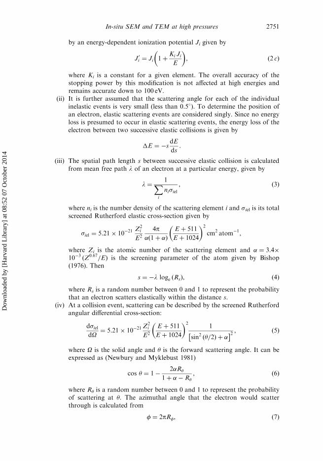
by an energy-dependent ionization potential Ji given by

J 0i ¼ Ji 1þ

Ki JiE

� �, ð2 cÞ

where Ki is a constant for a given element. The overall accuracy of thestopping power by this modification is not affected at high energies andremains accurate down to 100 eV.

(ii) It is further assumed that the scattering angle for each of the individualinelastic events is very small (less than 0.5�). To determine the position ofan electron, elastic scattering events are considered singly. Since no energyloss is presumed to occur in elastic scattering events, the energy loss of theelectron between two successive elastic collisions is given by

�E ¼ �sdE

ds:

(iii) The spatial path length s between successive elastic collision is calculatedfrom mean free path l of an electron at a particular energy, given by

l ¼1X

i

ni�iel, ð3Þ

where ni is the number density of the scattering element i and �iel is its totalscreened Rutherford elastic cross-section given by

�iel ¼ 5:21� 10�21 Z2i

E2

4p�ð1þ �Þ

E þ 511

E þ 1024

� �2

cm2 atom�1,

where Zi is the atomic number of the scattering element and � ¼ 3:4�10�3

ðZ0:67=EÞ is the screening parameter of the atom given by Bishop(1976). Then

s ¼ �l loge ðRsÞ, ð4Þ

where Rs is a random number between 0 and 1 to represent the probabilitythat an electron scatters elastically within the distance s.

(iv) At a collision event, scattering can be described by the screened Rutherfordangular differential cross-section:

d�ieldO

¼ 5:21� 10�21 Z2i

E2

E þ 511

E þ 1024

� �21

sin2 ð�=2Þ þ �� �2 , ð5Þ

where O is the solid angle and � is the forward scattering angle. It can beexpressed as (Newbury and Myklebust 1981)

cos � ¼ 1�2�R�

1þ �� R�

, ð6Þ

where R� is a random number between 0 and 1 to represent the probabilityof scattering at �. The azimuthal angle that the electron would scatterthrough is calculated from

� ¼ 2pR�, ð7Þ

In-situ SEM and TEM at high pressures 2751

Dow

nloa

ded

by [

Har

vard

Lib

rary

] at

08:

52 0

7 O

ctob

er 2

014

where R� is a random number between 0 and 1 to represent the probabilityof scattering at the angle �.

(v) Finally for a multielement scattering medium (e.g. an organic substance),instead of constructing an average atom of the medium, we consider thatthe sum of the probabilities Pi that electrons are scattered by all then elements present is given by

Xi

Pi ¼ 1:

The probability that the element h scatters is given by

Ph ¼ nh�iel: ð8Þ

So to select an element, a random number Relement between 0 and 1 isgenerated. If the condition

Xh�1

i¼0

Pi <Relement4Xhi¼0

Pi ð9Þ

is satisfied, then h is chosen. If it is not satisfied, the procedure is repeateduntil it does. For a multilayer problem, for example a layer of water overa layer of bone, the Monte Carlo process is carried through to the bottomlayer, changing the relevant parameter, i.e. the number density, or theatomic number at the boundary between the layers.

2.1.1. Characteristic X-ray emissionInelastic collisions along the step length of each interelastic collision can be

evaluated if it is assumed that the number of photons of X-rays of the characteristicwavelength is proportional to the inner-shell ionization cross-section. The inner-shellionization cross-section is that due to Bethe (Joy 1986):

�x ¼ 6:51� 10�20 nsbsEEc

logcsE

Ec

� �, ð10Þ

where ns is the number of electrons in the shell, bs and cs are constants and Ec (keV)is the critical ionization energy of the characteristic X-ray line. The values of Ec usedherein are those tabulated by Goldstein et al. (1981). The total X-ray yield along thestep s is given by

Is ¼ �xni!s,

where ! is the fluorescence, that is the number of photons per ionization. It shouldbe noted that the above emission is assumed to be isotropic (Ding et al. 1994).

From the above the relative yields at the detector can be estimated by employingBeers’ law of absorption

�

�

� �energy

specimen

¼Xi

�

�

� �energy

Ci , ð11Þ

where Ci is the percentage weight of the element i.

2752 J. Shah

Dow

nloa

ded

by [

Har

vard

Lib

rary

] at

08:

52 0

7 O

ctob

er 2

014

} 3. Applications to scanning electron microscopy

Normally the range of primary electron energy encountered in the scanningelectron microscope is 0.5–50 keV. The formulations developed in } 2 can thereforebe applied.

3.1. Testing convergence with the modelFirst of all, to determine the optimum number of calculations needed for

convergence, a simulation was run for a two-layer specimen, namely a water layer(5 mm) on top of the bone layer. The fact that a good statistical convergence occursfor the value of the back-scattering coefficient (BC) at about 350 000 trajectories isshown in figure 1. Unless otherwise stated, approximately 400 000 trajectories weresimulated to obtain the results described.

3.2. Modelling of multilayer specimensIn a typical HPSEM set of conditions there are liquid and vapour phases of

water present over the specimen. Figure 2 schematically shows the multilayer modelused to take account of the above.

3.2.1. Modelling of boneThere are many types of bone. For the purpose of mixed-free-element represen-

tation of bone in the Monte Carlo calculations it is important to know the composi-tion. The mineral content of a bone can be expressed as the volume fractionalmineral (VFM). For the results described below the modelled bone was hydratedbone with 0.3VFM (corresponding to a young bone). Following Howell and Boyde(1994) and Shah and Joyce (1996), it was assumed that there was no soft tissue in thebone. The chemical composition of hydrated 0.3VFM bone is given in table 1.

0

0.1

0.2

0.3

0.4

0.5

0.6

0.7

0.8

0.1

0.3

0.5

0.7

0.9

1.1

1.3

1.5

1.7

1.9

2.1

2.3

2.5

2.7

2.9

3.1

3.3

3.5

3.7

3.9

4.1

4.3

4.5

log (number of trajectories)

Bac

k S

catt

ered

Co

effi

cien

t

Figure 1. Variations in the BC against log (number of trajectories) showing convergence.

In-situ SEM and TEM at high pressures 2753

Dow

nloa

ded

by [

Har

vard

Lib

rary

] at

08:

52 0

7 O

ctob

er 2

014

3.3. Back-scattered electron emission from bilayer Specimens

3.3.1. Water vapour layer over bonePowell et al. (1997) considered a static water vapour layer at the saturated

vapour pressure of water at the ambient temperature (20�C) over bone. These aretypical HPSEM conditions. Calculations (without taking into account the kineticnature of the gas and the effect of gas ion movement) were performed for a 20 keVbeam passing through 5000 mm (5mm) of water vapour. Figure 3 shows the profileof the resultant scattered beam. It can be seen that the beam maintains a sharp peakat the original point of focus and a very-low-density distribution of electrons wellbeyond a 200 mm radius. This means that, according to the Rayleigh definition ofresolution, the inherent image resolution is maintained even after the beam hasscattered through the water vapour layer. However, it must be noted that thenumber of electrons in the focal peak is reduced to about 10% of the incidentelectrons. Thus the image contrast in these conditions will be drastically reducedand the image in these conditions will be very noisy. This in turn can reduce theresolution in practice.

Figure 2. Schematic diagram of the representation of the three-layer model for Monte Carlosimulations including the material under study (specimen), present in HPSEM.

Table 1. Chemical composition ofhydrated 0.3VFM bone.

ElementAmount of element

(wt%)

H 0.016C 0.180N 0.068O 0.418P 0.095S 0.017Ca 0.205

2754 J. Shah

Dow

nloa

ded

by [

Har

vard

Lib

rary

] at

08:

52 0

7 O

ctob

er 2

014

3.3.2. Liquid water layer on bone—the critical depth of waterElectron scattering in a liquid layer of water on the specimen is much stronger

than that in the water vapour. One can define an important parameter, namely thecritical depth (CD) of water, exactly in the same way as that defined for the cellulose–water bilayers (Shah et al. 1994). The plots of the number of back-scattered electrons(BSEs) emerging out of the water from within the bone and that from the actualwater layer are shown in figure 4 (a). The point of intersection between thetwo curves is defined as the CD of water (Shah et al. 1994). At the CD the numberof BSEs from the bone is the same as that from the water layer. Knowledge of theCD enables one to adjust the optimum depth of water for better protection fromdehydration and at the same time to obtain a reasonable signal-to-noise ratio fromthe specimen. Figure 4 (b) shows the variation in the CD with the incident beamenergy. This graph, with other criteria, can be used to decide which incident beamenergy should be used. Figure 5 shows the percentage of BSEs, emitted from withina linear distance from the point of incidence of the beam, from the hydrated boneunder different depths of a water layer. The graphs in figure 5 indicate the achievableresolution of a knife edge for different depths. It can be clearly seen that for depthsof water greater than 0.2 mm the resolution decreases very rapidly with the increasingdepth. A similar conclusion is also reached from the calculations for bone with twolayers on the top.

3.4. Back-scattered electron calculations of bone with two layers on the topWhile performing HPSEM for a hydrated specimen a more realistic situation

is that there will be three layers present (figure 2), namely a layer of water vapour onthe top, then a layer of water and bone at the bottom. Calculations were performedfor hydrated bone (infinite thickness), a water layer of variable thickness on the topof the bone and a layer of water vapour with a constant thickness of 2000 mm ata pressure of 2266 Pa. By comparing figure 6 (a) with figure 6 (b), one can see howthe radial distribution of BSE changes for a sample with water of depth from 0.2 to

0

500

1000

1500

2000

2500

1 19618317015714413111810592796653402714

Radial distance from the point of incidence (nm)

No

. of

BS

E

Figure 3. Number of electrons back-scattered through water vapour 5000 mm (5mm) deepat 20�C and at the saturated water vapour pressure of 17Torr (2266 Pa).

In-situ SEM and TEM at high pressures 2755

Dow

nloa

ded

by [

Har

vard

Lib

rary

] at

08:

52 0

7 O

ctob

er 2

014

0.5 mm. The BSE peak from the bone with a 0.2 mm water layer is much higherand sharper than that with a 0.5 mm water layer.

More importantly, the percentage of BSEs from the water layer 0.2 mm thick isof similar magnitude to that from the bone. Similar calculations were carried out forthe range of 0.1–0.9 mm. They show that the peak height varies linearly with thedepth and that no BSEs come out from the bone if the water depth is 0.9 mm. Thesecalculations assert that the ideal depth of the water layer is 0.2 mm, because the BSEcontribution of both the layers is small and the radial distribution of the BSEs isthe sharpest. At these conditions the detector needs to be 5mm in radius if it isplaced just above the water vapour layer (i.e. slightly more than 2mm above thebone surface). These findings are very similar to those for a cellulose–water system(Shah et al. 1994, Shah and Weare 1995).

3.4.1. Variations with the depth of the water vapour layerFigures 6 (c) and (d ) show the radial distributions of BSEs for water vapour layer

depths of 1000 mm and 4000 mm respectively. Water layer depths in both cases arethe same (0.2 mm). It is clear from theses that the BSE yield from the bone decreasesby a factor of about 10 for increase in the depth by a factor of 3. From these andother calculations it is concluded that, generally, the increase in the depth of thewater vapour layer causes the following effects:

(i) a decrease in the number of BSEs from the bone, which reach the top of thewater vapour layer;

(ii) a decrease in of the average energy of the above BSEs;

0

2

4

6

8

10

12(b)

0 605040302010

Beam energy (keV)

Cri

tica

l Dep

th

Figure 4. (a) Number of BSEs emerging out of the layer assembly from layer 1 (water) andlayer 2 (hydrated bone) (incident beam energy, 20 keV). The depth at the point ofintersection between the two curves is defined as CD. (b) Variation in the CD of waterwith beam energy, for a hydrated 0.3VFM bone specimen.

0

2000

4000

6000

8000

10000

12000(a)

0 0.5 1 1.5 2 2.5 3 3.5 4

Depth (microns)

Nu

mb

er o

f B

SE

BSE from layer 1 BSE from layer 2

2756 J. Shah

Dow

nloa

ded

by [

Har

vard

Lib

rary

] at

08:

52 0

7 O

ctob

er 2

014

00 2000 4000 6000 8000 10000

100

200

300

400

500

600(a)

Fre

quen

cy

Radius (microns)

BSEs from vapourBSEs from waterBSEs from bone

Figure 6. (a) Radial distribution of BSEs from three layers, namely bone, water (0.2 mm) anda water vapour layer (2000mm) (incident electron energy, 10 keV). The peak from thebone is much higher and sharper than those from the water layer and the water vapourlayer. (b) BSE radial distribution from bone, water (0.5 mm) and water vapour layer(2000mm) (incident beam energy, 10 keV). (c) Radial variations in the BSE frequenciesfrom bone, water (0.2 mm) and water vapour layer (1000mm) (incident beam energy,10 keV). (d ) Radial variations in the BSE frequencies for bone, water and watervapour layers (incident beam energy, 10 keV). The depth of the water layer is0.2mm and water vapour is 1000 mm.

0.0%

20.0%

40.0%

60.0%

80.0%

100.0%

120.0%

2 12 22 32 42 52 62 72 82 92 102 112 122 132 142 152 162 172 182 192

Linear distance from the point of incidence (nm)

% B

SE

-hyd

rate

d b

on

e- f

rom

wit

hin

th

e lin

ear

dis

tan

cefr

om

th

e p

oin

t o

f in

cid

ence

0.1

0.2

0.3

0.5

0.8

1

Figure 5. Percentage of BSEs emitted from within a linear distance from the point of inci-dence of the beam from the hydrated bone under different water layer depths (incidentbeam energy, 20 keV). These graphs also indicate achievable knife edge resolution fordifferent depths.

In-situ SEM and TEM at high pressures 2757

Dow

nloa

ded

by [

Har

vard

Lib

rary

] at

08:

52 0

7 O

ctob

er 2

014

-200

0

200

400

600

800

1000

1200

1400(c)

0 80007000600050004000300020001000

Radial Distance of BSE's (microns)

Fre

quen

cy o

f BS

E's

BSE's from VapourBSE's from WaterBSE's from Bone

Figure 6. (continued )

0

50

100

150

200

250(b)

0 10000900080007000600050004000300020001000

Radius (microns)

Fre

qu

ency

BSE from vapourBSE from water

BSE from bone

Figure 6. (continued )

2758 J. Shah

Dow

nloa

ded

by [

Har

vard

Lib

rary

] at

08:

52 0

7 O

ctob

er 2

014

(iii) a decrease in the number of BSEs from the water layer reaching the top;(iv) an increase in the ‘broadness’ of the radial frequency distribution of the BSE

energies from the bone, water and water vapour layers, presumably becausethe incident beam would spread as it passes through the vapour layer on tothe bone.

0

100

200

300

400

500

600

0 600040002000 8000 10000

Radius (microns)

Fre

quen

cy

water depth = 0.1 micronswater depth = 0.2 micronswater depth = 0.3 micronswater depth = 0.5 micronswater depth = 0.6 micronswater depth = 0.7 microns

Figure 7. Radial distribution from bone and different water layer depths (incident beamenergy, 10 keV).

0

50

100

150

200

250(d)

0 2000 4000 6000 8000 10000

Radius (microns)

Fre

qu

ency

BSE from vapourBSE from waterBSE from bone

Figure 6. (continued )

In-situ SEM and TEM at high pressures 2759

Dow

nloa

ded

by [

Har

vard

Lib

rary

] at

08:

52 0

7 O

ctob

er 2

014

3.4.2. Dependence on the depth of the water layerThe variation in the frequency curves of the BSEs originating in the bone layer

was also examined for different water layer depths with the water vapour depth keptconstant at 2000 mm. This is shown in figure 7. It is noted that there is a steadyprogression from having no BSEs at 0.9 mm to the maximum at 0.1 mm. The factthat there are no BSEs from bone when the water depth is 0.9 mm agrees with thedata for cellulose (Shah et al. 1994). This means that if one were to cover a specimenwith this depth of water, there would be no information relating to the specimenBSEs. One can also see that the curves for depths of 0.1 and 0.2 mm are very similarwith respect to the total BSEs from the bone, meaning that the masking effects ofthe water are similar. Surprisingly, the distribution is wider for a depth of 0.1 mmthan for a depth of 0.2 mm. This means that resolution would be slightly worse inthis case. It is interesting to note that the width of the curves for bone varies onlyslightly. The widths of the peaks points to an important consideration in the detectordesign. The detector for HPSEM needs to be only 5mm in radius if placed at thesurface of the vapour layer. Figure 7 gives an idea of the kind of resolution that canbe obtained for bone under water layers of various depths.

3.4.3. Dependence of back-scattered electrons on beam energyThe effect of increasing incident electron energy is shown in figure 8. It is

generally concluded that the increasing beam energy causes the following effects:

(i) an increase in the number of BSEs from the bone layer reaching the top ofthe water vapour which is roughly proportional to the square of the energyof incident electrons;

(ii) a decrease in the number of BSEs from the water and water vapour layers;(iii) an increase in the energy of the BSEs from bone;(iv) an increase in the broadening of the radial distribution.

3.5. Characteristic X-ray generation from the bone layerCalculations were performed for specimens with a single layer of bone and

bilayers of water and bone at the incident electron energy of 20 keV. Figure 9

-100

0

100

200

300

400

500

0 5 10 15 20 25

Energy (keV)

Fre

qu

ency

5 keV beam

10 keV beam

15 keV beam

20 keV beam

Figure 8. Variations in the BSEs from bone with incident beam energy (water layer depth,0.2mm; water vapour layer depth, 1000mm).

2760 J. Shah

Dow

nloa

ded

by [

Har

vard

Lib

rary

] at

08:

52 0

7 O

ctob

er 2

014

shows radial profiles of the frequency of characteristic X-ray photon emission fromthe elements C, N, O, P, S and Ca present in bone. It is clear therein that theresolution differs from element to element. Generally the distribution broadensout as the atomic number increases.

0.00%

1.00%

2.00%

3.00%

4.00%

5.00%

6.00%

7.00%

8.00%

9.00%

10.00%

100 200 300 400 500 600 700 800 900 1000

Depth of water (nm)

% o

f ca

lciu

m X

-ray

s em

itte

d f

rom

wit

hin

rad

ius

10nm 20nm 30nm 40nm 50nm

Figure 10. Dependence of the spread of characteristic Ca X-rays from bone on the depth ofwater (incident energy, 20 keV). Calculations were performed for five different radiiemitting X-rays, listed above the plots.

0

1000

2000

3000

4000

5000

6000

7000

50 350

650

950

1250

1550

1850

2150

2450

2750

3050

Radial Distance from probe focus point (nm)

Nu

mb

er o

f p

ho

ton

s (r

elat

ive)

Carbon

Nitrogen

Oxygen

Phosphorus

Sulphur

Calcium

Figure 9. Radial distribution frequency of characteristic X-ray photons from the hydratedbone plotted against the radial distance from the point of incidence (incident energy,20 keV).

In-situ SEM and TEM at high pressures 2761

Dow

nloa

ded

by [

Har

vard

Lib

rary

] at

08:

52 0

7 O

ctob

er 2

014

The effect of water layer on the spread of characteristic X-rays of Ca for fivedifferent emitting radii is shown in figure 10. It is apparent therein that the spreadcan be appreciable. By estimating the distribution of the Ca signal around thepoint of incidence (the resolvable radius), it is possible to compare the spatial resolu-tion of Ca with that of the BSE image. Figure 11 shows the plots of the variations inthe resolvable radii for Ca X-rays, BSEs and the incident beam for different depthsof water layer. It may be inferred from the calculations that the microanalyticalresolution in the presence of water is marginally better than that for the BSEs.The amount of Ca signal from the resolved image area shows a d2 dependence,where d is the depth of the water above the specimen. It should be appreciatedthat, while the resolution changes with water depth, the interaction volume roughlystays the same and so the proportion of the Ca signal coming from the imagearea increases as the resolvable radius increases. Finally it must be noted that inthe above results the amount of characteristic X-ray resolution depicted here ismuch better than that obtainable in practice since the calculations here do nottake into account the X-rays generated from a large ‘skirt’ of the small number ofelectrons per area around the point of incidence of the beam. However, it can alsobe inferred that there should be a significant difference in the count from the mainphoton peaks due to the incident electrons and those from subsidiary peaksproduced by the scattered electrons.

} 4. Extension of the single-scattering model for high-energy electrons

For transmission electron microscopy (TEM), generally, electrons with energyrange 100 keV–2MeV are employed. Previously, a multiple-scattering approxima-tion has been used for high-energy electrons. In this approximation, one makes eachand every electron travel the same distance in the material before coming to rest.

In the multiple-scattering approximation dE/dS is still obtained from the modi-fied Bethe equation (Joy and Luo 1989). Thus a screened Rutherford section is usedbut it is in a different form; it uses an impact parameter b to represent the projectednearest distance of closest approach of the electron to the scattering nucleus. Theseassumptions are drastic. Although they give the right value of BC the energy dis-

0

5

10

15

20

25

100 300 500 700 900 1100

Depth of water covering specimen (nm)

% C

a X

-ray

s em

itte

d f

rom

wit

hin

res

olv

able

rad

ius

x-rays resolution BSE resolutionbeam resolution

Figure 11. Comparison of resolutions of the incident beam, the BSEs and the characteristicX-rays of Ca from bone obtainable for various depths of the water layer (incidentenergy, 20 keV).

2762 J. Shah

Dow

nloa

ded

by [

Har

vard

Lib

rary

] at

08:

52 0

7 O

ctob

er 2

014

tribution is not in agreement with the experimental data. Furthermore, in themultiple-scattering model, at 100 keV, the step length is about 1 mm and is too grainy(too coarse). The quality of the results is better if a finer step size is achieved. In thesingle-scattering model the step length is in the range of a few nanometres to a fewtens of nanometres. To take into consideration the relativistic effects at high energy,the single-scattering model has been extended to high-energy electrons (up to2.2MeV) using the recently developed equation by Kawrakow and Rogers (2002):

d�rel:eld�

¼2pr20Z

2

�2� � þ 2ð Þ

1

1� �þ 2ð Þ2, ð12Þ

where � is the electron velocity in units of c (the velocity of light), � is the kineticenergy in units of the electron mass, r0 is the Bohr radius, �¼ cos (�) and is ascreening parameter (Kawrakow and Rogers 2002). Equation (12) thus representsthe corrected screened Rutherford differential scattering cross-section for high-energy electrons.

For calculating the energy loss the continuous, a slowing-down approximationcan still be used. However, instead of using the Bethe equation (1); the calculationsare performed with the parametric fit for the energy loss provided by Gupta andGupta (1980) along the lines suggested by Berger and Seltzer (1974):

�1

�

dE

dS

� �total

¼ SZ þ 1:3230ð Þ2

aZþb � 1, ¼

�

mc2þ 1 ð13Þ

where � is the kinetic energy of the incident electrons, and S, a and b are the fittingparameters.

4.1. Application of relativistic calculationsAs the equations in } 4 have not been applied before to either scanning electron

miscroscopy (SEM) or TEM, calculations were performed using equations (12)and (13) for low and high energy values and compared with the calculations madeby using (low-energy) equations (1) and (5). At medium energies both calcula-

50 450400350300

non-relativistic: BCnon-relativistic: TCrelativistic: BCrelativistic: TC

250200150100

0.0

0.2

0.4

0.6

0.8

1.0

Co

effi

cien

t

Energy [keV]

Figure 12. Comparison of the variations in the BC and the TC of a 0.3VFM bone slice 50 mmthick calculated by relativistic and non-relativistic equations.

In-situ SEM and TEM at high pressures 2763

Dow

nloa

ded

by [

Har

vard

Lib

rary

] at

08:

52 0

7 O

ctob

er 2

014

tions should be expected to give the same values for the BC and the transmissioncoefficient (TC).

Figure 12 shows that for a 0.3VFM bone slice (50 mm thick) the variations inthe BC and TC with energy for relativistic and non-relativistic cases agree at lowenergies below 100 keV. While comparing these figures, one should remember thatthe reliability of the non-relativistic calculations decreases as the energy increases.The same applies for the reliability of the relativistic calculations as theenergy decreases. In the energy range 50–200 keV, both relativistic and non-relativ-istic values can be compared with some confidence. It is apparent that non-relativ-istic calculations for TC give significantly higher values than those given byrelativistic calculations. Thus it appears that, for energies greater than 70 keV,non-relativistic calculations may overestimate TC. This should be further checkedfor other specimens.

} 5. Discussion and conclusions

It has been conclusively shown that the single-scattering approximation can befruitfully applied to gain information on complex organic substances. The calcula-tions can correctly predict the behaviour of various parameters with energy.Unfortunately, the experimental data on the BC, X-ray yield and other parametersare scanty but it is hoped that this presentation will stimulate interest in generatingmore data. It is important to note that the free-element modelling of a complexsubstance and a random choice of a scattering atom has not been widely appliedto very complex biosubstances. We can directly compare the results of the BC ofbone obtained here with those obtained by constructing an average atom of bone(Howell and Boyde 1994) because the composition of bone used here was the sameas the compositions used by the above researchers. The calculations reported hereshow that the BC decreases with the increasing beam energy in the range commonlyused in SEM. This behaviour is commonly observed across a wide range of materi-als. The actual values of the BC obtained herein are, generally, consistently differentfrom those of Howell and Boyde. It is possible that this difference may well be dueto the difference between two models in setting up scattering cross-sections. It isdifficult to say at this moment in time which model will provide a closer agreementwith the experimental values of a wide variety of complex substances.

The single-scattering Monte Carlo modelling can be extended to high-energyelectrons for the purpose of TEM to take into account the relativistic effectsby a new approach adapted herein. Although the calculations presented here wererestricted to about 450 keV, the equations can be applied to higher beam energiesup to about 2.2MeV.

Multielement multilayer modelling of a complex specimen clearly shows thatthe effects of scattering due to the necessary experimental conditions to keep thespecimen fully hydrated can be successfully studied. It has been shown that, bycontrolling the depth parameters of water and water vapour and subject to otherrestrictions cited, one can obtain not only a high (BSE) image resolution but also acomparable resolution in elemental mapping and chemical analyses at the microme-tric and nanometric levels.

Acknowledgements

Many thanks are due to Stefan Hoppe, Ben Hartwright, Andrew Stals, DavidJoyce and Harry Powell for contributions to the calculations.

2764 J. Shah

Dow

nloa

ded

by [

Har

vard

Lib

rary

] at

08:

52 0

7 O

ctob

er 2

014

References

Berger, M. J., and Seltzer, S. M., 1964, Nuclear Science Series Report 39, NationalAcademy of Science and National Research Council (Washington, DC);1974, Special Publication, NASA-Sp-3012, National Aeronautics and SpaceAdministration.

Bethe, H. A., 1930, Ann. Phys. Leipzig, 5, 325.Bishop, H. E., 1976, Monte Carlo Calculations in Electron Microscopy, National Bureau of

Standards Special Publication 460, edited by K. F. G. Heinrich, D. E. Newbury andH. Yakowitz (Washington, DC: US Department of Commerce, NBS), p. 5.

Ding, Z.-J., Shimizu, R., and Obori, K., 1994, J. appl. Phys., 76, 7180.Goldstein, J. I., Newbury, D. E., Echlin, P., Joy, D. C., Fiory, C. and Lifshin, E., 1981,

Scanning Electron Microscopy and X-ray Microanalysis (New York: Plenum), p. 641.Gupta, S. K., and Gupta, D. K., 1980, Jap. J. Appl. Phys., 19, 1.Howell, P. G. T., and Boyde, A., 1994, Bone, 15, 285.Joy, D. C., 1988, Inst. Phys. Conf. Ser., 93, 1.Joy, D. C., and Luo, S., 1989, Scanning, 11, 176.Kawrakow, I., and Rogers, D. W. O., 2002, NRCC Report PIRS-70.1 (Ottawa, Canada:

National Research Council of Canada), p. 82.Knoll, M., and Ruska, E., 1932, Z. Phys., 78, 318.Matsukawa, T., Murata, K., and Shimizu, R., 1973, Phys. Stat. sol. (b), 55, 371.Newbury, D. E., and Mykelbust, R. L., 1981, Analytical Electron Microscopy, edited by R.

H. Gleiss (San Francisco Press), p. 91.Powell, H. R., Hollis, K. J., and Shah, J. S., 1997, Inst. Phys. Conf. Ser., 15., 15, 245.Shah, J. S., 1995, Proceedings 6th European Conference on Applications of Surface and

Interface Analysis ECASIA 95, edited by H. J. Mathieu, B. Reihl and D. Briggs(New York: Wiley), p. 345.

Shah, J. S., Durkin, R., and Weare, J. R., 1994, Electron Microscopy, vol. IIIB, Applicationto Biological Sciences, Les Ulis: Les Editions de Physique, p. 811.

Shah, J. S., and Joyce, D. W. H., 1996, Proceedings of the European Congress on ElectronMicroscopy, Dublin, Ireland, 1996 (Brussels: Committee of European Societies ofMicroscopy), pp. 1–131.

Shah, J. S., and Weare, J. R., 1995, Proceedings 6th European Conference on Applications ofSurface and Interface Analysis ECASIA 95, edited by H. J. Mathieu, B. Reihl and D.Briggs (New York: Wiley), p. 42.

In-situ SEM and TEM at high pressures 2765

Dow

nloa

ded

by [

Har

vard

Lib

rary

] at

08:

52 0

7 O

ctob

er 2

014