APPLICATIONS OF HIGH RESOLUTION SOLID STATE … · James P. Wi ghbt'Jrn ,!1fa'rry C. Dorn August,...
187
APPLICATIONS OF HIGH RESOLUTION SOLID STATE CARBOtJ-13 NMR TO THE STUDY OF MULTICOMPONENT POLYMER SYSTEMS by Tso-Shen Lin Dissertation submitted to the Graduate Faculty of the Virginia Polytechnic Institute and State University in partial fullfillment of the requirements for the degree of DOCTOR OF PHILOSOPHY in Chemistry APPROVED: Thomas C. Ward, Chairman James E. McGrath Garth L. Wilkes James P. Wi ghbt'Jrn ,!1fa'rry C. Dorn August, 1983 Virginia
Transcript of APPLICATIONS OF HIGH RESOLUTION SOLID STATE … · James P. Wi ghbt'Jrn ,!1fa'rry C. Dorn August,...

APPLICATIONS OF HIGH RESOLUTION SOLID STATE CARBOtJ-13
NMR TO THE STUDY OF MULTICOMPONENT POLYMER SYSTEMS
by
Tso-Shen Lin
Dissertation submitted to the Graduate Faculty of the Virginia Polytechnic Institute and State University
in partial fullfillment of the requirements for the degree of
DOCTOR OF PHILOSOPHY
in
Chemistry
APPROVED:
Thomas C. Ward, Chairman
James E. McGrath Garth L. Wilkes
James P. Wi ghbt'Jrn ,!1fa'rry C. Dorn
August, 1983
B1acksburg~ Virginia

To My Parents
ii

ACKNOWLEDGEMENTS
The author is pleased to express his appreciation to Dr. Thomas ·C.
Ward for his guidance and support of this work. Appreciation is
extended to Ors. James E. McGrath, Garth L. Wi 1 kes, James P. Wightman,
Harry C. Dorn for their willingness to serve on the graduate committee.
He also wishes to thank Ors. Harold M. Bell and Brian E. Hanson for
serving on the examining committee and their time in going over the
dissertation.
The author would also like to thank many people in the PMIL and
Chemistry Department at VPI and SU. Especially, Mr. Tom Glass for his
assistance in starting the "magic angle" solid state NMR experiments,
Or. Daniel P. Sheehy, Dr. Oillip K. Mohanty and Mr. Pradip K. Oas for
their helpful discussions. Finally, he wishes to thank Mrs. Debbie
Farmer and Mrs. Diann Johnson for typing this dissertation.
iii

Table of Contents
Page
ACKNOWLEDGEMENTS •••••••.••••.•.••....•••••••••••••.••••••••...•. iii
LIST OF FIGURES . • • . . • • • • • • • . • . • • • • • • • • • • • • • • • • • • • • . • • • • . • • • • • • • • ix
L I ST OF TABLES ••.•••••••••.••..••.•••••••.•••.••.••.••. ., • • • • • • . • xi
Chapter I. INTRODUCTION AND LITERATURE SURVEY................... 1
I. INTRODUCTION ............................................ 1
II. HIGH RESOLUTION SOLID STATE NMR •••••••••••••••••••••. 3
A. Fundamentals of Nuclear Magnetic Resonance .•••... 3
l. The N~1R Phenomenon • • • • • • • • • • • . • • • • • • • . • • . • .. • • 3
2. Fourier Transform NMR .•••••••••.•••••••••.••• 9
3. Relaxation Processes .••••.••.•.•.•••••••••••. 15
4. Relaxation Time Measurements .•.••••••••••••.• 22
5. The NMR Parameters • • . • • . • . • . . . • • • • • • • • • • • . . • • 25
B. Introduction to Solid State NMR ..••••••••.••..••• 29
C. The Resolution Problem: Sources of Line-Broadening and Methods for Their Removal .•••••••• 30
1. Magic Angle Spinning ••.••••.••••..•••.•.••.•• 34
2. Decoupling •••.•.•.•..••••.•••••..•••..•••.••• 38
3. Factors Affecting Resolution in High Resolution Solid State NMR •••••••••.••••••••• 40
D. The Sensitivity Problem and Its Solution .•..•••.• 42
1. General Considerations and Definitions ••••••• 43
2. Spin-Lattice Relaxation in the Solid State ••. 44
i \I
Page
3. Relaxation in the Rctatir.g Frame .•••••••.•••• 46
4. Cross Polarization ••••••••••.•••••••••••••••• 48
5. Relaxation Time Measurements - The Cross Polarization Methods •••••••••••••••••••••••• 53
III. MULTICOMPONENT POLYMER SYSTEMS ••••••.•.••••.•••••••. 55
A. Classification
1. Copolymers
2. Polyblends
3. ·composites
..................................
..................................
..................................
..................................
55
55
56
57
B. Polymer-Polymer Miscibility ····~················ 57 1. General Thermodynamics of Polymer-Solvent
and Polymer-Polymer Systems ••••••••••••••••• 60
2. Stability and Phase Separation Phenomena • • • • 62
3. Solubility Parameter Aoprcach •••.••••••••••• 65
4. Statistical Mechanical Approach ••••••••••••• 66
5. Thermodynamics of Block Copolymer Systems 67
6. Methods for Determining Polymer-Polymer Mi sci bi 1 i ty .... ., . . . . . . . . . . . . . . . . . . . . . . . . . . . . 69
Chapter II. CHARACTERIZATION OF STYRENE-ISOPRENE-STYRENE TRIBLOCK COPOLYMERS AND POLYURETHANES ••••••••.•••• 74
I. INTRODUCTION • • • • • • • • • • • • • • • • • • • • • • • • • • • • • a • • • • • • • • • • 74
II. EXPERIMENTAL Cf ....................................... . 76
A. Samples .................. ,. •.....••.•• "........... 76
B • NMR • • • • • • • • • • • • • • • • • • • • • • • • • • • • • • • • • • • • • • • • • • • • • 78
v

III. RESULTS
A. SIS
............................................. Copolymers ................................. .
page
81
81
1. General Description of Spectra ••.••••••••••• 81
2. Mobile Domains ••..•...••.•••...••.•...•..•.. 83
3. Rigid Domains ••••••••••••••••••••••••••.•.••• 92
B. Polyurethane ••••••••.••••••.••••••••••••.•••••••• 92
1. General Description of Spectra ••••••••••.•.•• 92
2 • T 1 Measurements ..••••••••.•• ,, • • • • • • • • • • • • • • • • • 96
3. Cross Polarization Intensity as a Function of Contact Time •...•.•....•.••.•••......•.... 101
IV. DISCUSSION ••••••••••••••••••••••••••••••••••••••••.•• 101
A. SIS Copolymers ••••••••.••••••••••.•••••••••••.••• 101
1. Phase Separation-Nature of Domain Boundaries •••••••.••••••••••••••••••••••••••• 101
2. Molecular Motion in the Mobile Domains ••••••• 105
3. Molecular Motion in the Rigid Domains •••••••• 108
B. Polyurethane .............•••.•.................•. 109
1. Phase Separation •......•...•..•••.•..•....•.. 109
2. Molecular Motions 110
V. CONCLUSIONS •••••••••••.•••.•••••••••••••••••••••••••• 113
Chapter III. COMPATIBILITY STUDIES OF POLYMER BLENDS CONTAINING POLY(VINYLIDENE FLUORIDE) ••••••••••••••••••••••••• 117
I. INTRODUCTION ••.•.•.••...•...•.•••.••.•••••••••••••••• 117
vi

page
II. EXPERIMENTAL ••••..•••...•.•...•.......••..•.•.••••••• 119
A. Sources and Characterization of Homopolymers ••••• 119
B. Preparation of Blends •••••••••••••••••••••••••••• 120
C. NMR .............................................. 121
D. DSC ............................................... 122
II I. RE SUL TS ............. • ................................ . 122
A. General Description of NMR Spectra and DSC Curves ••••••••••••.••••••••••••••.••••••••••••••• 122
B. Melting Point Depressions of PVF2 and NMR Signal Attenuations of Non-PVF2 Polymers in the Blends ••••••••••••••••••••••••••••••••••••••••••• 126
C. Carbon-13 Resolved Proton's Tip's •••••••••••••••• 130
IV. DISCUSSION ........................................... 139
A. Shifts of NMR Frequencies •••••••••••••••••••••••• 139
B. NMR Signal Attenuations and Degrees of Intermixing .. • . . . . . . . . . . . . . . . . . . . . . . . . . . . . • . • . . . . 139
1. PVFz/PMMA Blends .............................. 140
2. PVF2/PVAc Blends ............................. 143
3. PVF2/PVME Blends ............................. 145
4. NMR Signal Attenuations of Individual Carbons •••••••••••••••••••••••••••••.•••••••• 145
C. NMR Signal Attenuations and Magic Angle Spinning Rates ••••••••••••••••••••••••••••••••••• 146
D. NMR Signal Attenuations and Relaxation Times ••••• 153
E. NMR Signal Attenuations and Effect of Aging 156
F. NMR Signal Attenuations and Number of Accumulations ••..•••••••.•.•••.•••••••.••..•••.•• 156
vii
page
V. CONCLUSIONS •••••••••••••••.••••••••••••••••••••••.••• 157
VI. FUTURE WORK ·······"·································· 160 A. Variable Temperature Studies ••••••••••••••••••••• 161
B. Compatibility Studies Through Heteronuclei Other than Fluorine-19 ••..••••••.••••••••••.•••••• 161
C. Compatibility Studies by Varying Heteronuclear Dipolar Decoupling Power ••••••••••••••••••••••••• 162
LITERATURE CITED ~........................ .. . • • • • • • • • . • • . • . • • • . • . • 163
VITA •••O••·········································•••.t••••••••• 174
ABSTRACT
vii~
List of Figure~
Figure page
1. Motion of Magnetic Moment in the Rotating Frame of Reference.................................................. 8
2. Behaviour of the Dipolar Spin-Lattice T1 DD and Spin-Spin T2 OD Relaxation Times as a Function of the Correlation Times ~c for Interaction Between two Identical Spin 1/2 Nuclei Undergoing Isotropic Reorientation.............................................. 21
3. NMR Powder Patterns of Nuclei.............................. 31
4. Gibbs Free Energy of Mixing as a Function of Concentration in a Binary Liquid System Showing Partial Miscibility...... 63
5. Proton Dipolar Decoupled, Magic Angle Spinning 15.0 MHz C-13 NMR Spectra of the SIS 20-60-20H Copolymer............ 82
6. One Component, First Order Spin-Lattice Relaxation Behavior of the Isoprene Segments of the SIS 10-80-10 Copolymer..... 87
7. Static Spectra of the SIS 20-60-20H Copolymers............. 91
8. 13C T1 Measurement for the Styrene Segments of the SIS 30-40-§o Samples Cast from Hexane.......................... 94
9. Solution and Solid State C-13 NMR Spectra of the Polyester-MDI Polyurethane with 31 wt% MDI................. 95
10. One Component, First Order Spin-Lattice Relaxation Behavior of the Polyurethane with 31 wt% MDI........................ 100
11. DD-MAS-CP 15.0 MHz C-13 NMR Spectra of the Polyester-MDI Polyurethane Obtained at Various Contact Times............. 102
12. The 15.0 MHz DD-MAS Solid State C-13 NMR Spectra of Homopolymers ••.•.•••••••••••••••.••••••••.•••.••..••••..••• 123
13. Melting Point Depressions of PVF2 and NMR Signal Intensity Attenuations of PMMA in the PVF2/PMMA Blends ••••••••••••••• 124
14. DD-MAS-CP 15.0 MHz C-13 NMR Spectra of PMMA obtained at Various Contact Times •••••••••••••••••••••••••••••••••••••• 134
15. DD-MAS-GP 15.0 MHz C-13 NMR Spectra of the Melt-Extruded 25:75 PVF2/PMMA Blend Obtained at Various Contact Times.... 135
ix

Figure
16.
17.
18.
19.
20.
21.
13c NMR Signal Intensity for the Carbonyl Carbon of PMMA in the Homopolymer and in the Melt-Extruded 25:75 PVF2/PMMA Blend as a Function of Contact Time •••.••..••••••••••••••••
Schematic Summary of Crystallization and Interconversions of the Polymorphic Phases of PVF2 •.•..••••••••••••••.••••••
% Residual C-13 Resonance Intensities of PMMA in the MEK-Cast PVF2/PMMA Blends ••••••••••.••••••••••.•..•••••••••
% Residual C-13 Resonance Intensities of PMMA in the MEK-Cast, Melted and Quenched PVF2/PNMA Blends .••••••••••••
% Residual C-13 Resonance Intensities of PMMA in the DMF-Cast, Melted and Quenched PVF2/PMMA Blends ••••••••••••.
% Residual C-13 Resonance Intensities of PMMA in the Melt-Exturded PVF2/PMMA Blends ••••••.•••••.••••.•••••••••••
22. % Residual C-13 Resonance Intensities of PVAc in the
page
136
142
147
148
149
150
DMF-Cast PVF2/PVAc Blends.................................. 151
x

List of Tables
Table page
1. Polyblends............... .................................. 58
2. Composites ........................ ,,,.......................... 59
3. Composition of SIS Copolymers.............................. 77
4. 13c NMR T1 for the Isoprene Segments of Four SIS Copolymers............................................. 85
5. Data Analysis of the T1 Measurements of the Isoprene Segments in SIS Copolymers................................. 86
6. Bandwidths of the Isoprene Segments in SIS Copolymers (with MAS) • • • • • • • • • • • • • • • • • • • • • • • • • • • • • • • • • • • • • • • • • • • • • . • • • • • • • • • 89
7. Bandwidths of the Isoprene Segments in SIS copolymers (Static)................................................... 90
8. 13c NMR T1p Values for the Styrene Segments in Two SIS 30-40-30 Samples Cast from Different Solvents.............. 93
9. Assignment of Resonances in C-13 NMR Spectrum of the Polyester-MDI Polyurethane from DMSO-d6.................... 97
10 • 13c NMR T1 Values for the T\'IO Most Intense Peaks of the Polyester-MDI Polyurethane with 31 wt% MDI •••••••••••••••••
11. Relative 13c NMR Peak Intensities of the Polyurethane obtained at Various Experimental Conditions •••••••••••.••••
12. Calculations of the Residual ~MR Signal Intensities ••••••••
13. Residual NMR Signal Intensities of PMMA in the PVF2/PMMA Blends ••••••••••••••••••••••••.• o••••••••••••••••••••••••••
14. Residual NMR Signal Intensities of PVAc in the PVF2/PVAc Blends ••••••••••••••••••••••••••••••••••••••••.••••••••••••
99
112
125
127
128
15. Residual NMR Signal Intensities of PVME in the PVF2/PVME Blends ................................................ 3 •••••• 129
16. 13C NMR Signal Intensities of PMMA Obtained at Various Experimental Conditions.................................... 131
xi

Table page
17. 13c NMR Signal Intensities of the Melt-Extruded 25:75 PVFz/PMMA Blend Obtained at Various Experimental Conditions................................................. 132
18. Residual NMR Signal Intensities of PMMA in the Melt-Extruded 25:75 PVFz/PMMA Blend, Calculated from the CP Spectra with Various Contact Times......................... 133
19. PMMA C-13 Resolved Proton's Tlp Values of the Homopolymer and the PVF2/PMMA Blends................................... 137
20. Residual NMR Signal Intensities of PMMA in Two Melt-Extruded PVF2/PMMA Blends as an Effect of Sample Aging...................................................... 138
21. 13c NMR Signal Intensities of PMMA obtained at Various Number of Accumulations.................................... 158
xii
Chapter 1
INTRODUCTION AND LITERATURE SURVEY
I. INTRODUCTION
Growth of the ability to control and design the physical and
chemical properties of polymeric materials is one of the main reasons
that polymers have been making a profound impact on modern technology
and way of 1 ife. Many of the successes have been achieved through
applications of multicomponent polymer systems including copolymers.
polyblends and composites (1-6). Further advancement in polymer science
and technology depends in part on understanding the molecular origins of
macroscopic behavior. In this regard, techniques of nuclear magnetic
resonance (NMR) have made notable contributions. especially through the
high resolution spectra in the liquid state (7-10).
For years after the first successful detection of nuclear magnetic
si gna1 s 1 ate in 1945 (11, 12). high resolution NMR was almost a synonym
for proton magnetic resonance in the 1 i quid state. \~i th the advent of
commercial pulse Fourier transform NMR in the early 1970 1 s (13-15) and
subsequent developments in instrumentation, the NMR experiments became
accessible for essentially the entire periodic table (16). Carbon-13
NMR in solution (17-21). in particular, has been extensively employed to
investigate polymers (22-23). A high degree of resolution in carbon-13
spectra allcws studies which are usually unachievable in proton NMR
experiments. such as the quantitative data on stereochemical
configuration and copolymer sequence distribution, to be determined
(24). It also makes possible to obtain data on sidechain and backbone
1

2
reorientational motion through the measurement of spin-lattice,
spin-spin and nuclear Overhauser relaxation parameters for each carbon
(25,26).
In spite of the success of solution C-13 NMR. many interesting
properties of bulk polymers disappear if the samples are put into
solution. These are properties such as the degree of crystallinity,
chain axis orientation, and primary and secondary molecular relaxations.
Even aging processes as a function of chain scission and crosslinking
have been studied by pulsed solid state (proton and fluorine-19) ~JMR
through the measurements of second moments and other relaxation
parameters. The spectrum of a solid polymer in these cases usually
consists of a single broad resonance line having a full-width at half
height of tens of KHz, and is known as a broad-line NMR spectrum (8,
27-31).
It might be assumed that if a high re solution NMR spectrum of a
solid could be obtained, new details concerning the nature cf the solid
state of polymers might be uncovered. Recent advances in the techniques
of multiple-pulse experiments and high speed magic angle spinning of
samples have now made possible the partial realizaion of this goa1
(32-36). Commercial instruments for high resolution solid state NMR of
some nuclei of either low natural abundance or of small magnetic moment
became available in the late 1970's (37) •. ~ong them high resolution
C-13 NMR achieved by employing the techniques of magic angle spinning
and high power 13c-1H dipolar decoupling and cross polarization (the
CPMAS method) (36) has drawn the most attention in the characterization

3
of organic sol id polymers. The resolution of signals for individual
carbons having bandwidths in the range of 10-100 Hz for polymeric solids
not only made CPMAS attractive as an analytical technique for insoluble
and crosslinked polymers but also provided a method for obtaining new
information about solid state structure and dynamics at the atomic level
(23,30, 38-41).
The work reported in this dissertation concerned application of the
techniques of high resolution sol id state C-13 NMR to a number of
multicomponent polymer systems.· Specifically, of major concern were:
(1) the domain sturcture and molecular motion of two thermoplastic
elastomer systems, including a series of styrene-isoprene-styrene linear
triblock copolymers of various composit'ions, molecular weights and
sample histories, and a poly(ester)urethane based on polybutylene
adipate and 4,4'-diphenylmethane diisocyanate. (2) the compatibility of
polymer blends containing poly(vinylidene fluoride). including its
solution and mechanical bl ends with poly( methyl methacryi ate).
poly(viny1 acetate) and poly(vinyl methyl ether).
II. HIGH RESOLUTION SOLID STATE NMR
A. Fundamentals of Nuclear Magnetic Resonance (13-i6,42-46)
1. The NMR Phenomenon
Basic Theory
A nuclear magnetic moment placed in a magnetic field has an
interaction described by the Zeeman spin Hamiltonian.

4
H = -µ • H = -yP·H = -y~IzHc ( 1)
whereµ is the nuclear magnetic moment. P is the spin angular momentum
of the nucleus,~ is the Planck's constant divided by 2~. and H0 is the
static magnetic field which was chosen to be along the z-axis. I is the
spin quantum number and its value depends on the type of nucleus and
determines the maximum observable component of the nuclear angular
momentum:
Pmax = 1iI ( 2)
Thus, 1iiz is the component of the angular momentum along the z-axis. The
magnetogyric ratio y is:
µ y - -
p
and is a characteristic of the nucleus.
The eigenvalues of this system are:
E = -y1iH0m
where m ranges from -I to +I. while the energy separation betv1een
adjacent levels is
t.E = y1iH0 = hvo
where
( 3)
( LI. \ . J
( 5)

5
2rt
y = Ho
2rt ( 6)
is called the Larmor precessi or. frequency as described by the equation
of motion of the magnetic moment
dµ = yµ x H0 = (-yH0 ) x µ = w0 x µ
dt ( 7)
At equilibrium, the nuclei are populated among the energy levels
according to a Bal tzman distribution resulting in a net macroscopic
magnetization along the z-axis:
Mz = Mo = --------- Ho 3k 8TI ( 8)
where N0 is the number of nuc1ei per unit volume, T is the absolute
temperature and ks is the Boltzmann constant.
The Resonance Phenomenon
The equilibrium state of the magnetic nuclei in H0 can be disturbed
when a small magnetic field "Hi is applied (In practice H1 is a linear
radio frequency (RF) field oscillating in the x or y Cartesian
coordinates). perpendicular to H0 and rotating about H0 in the same
direction asµ at frequency v. Resonance is attained when the
frequency ofl:fi exactly equals v 0 :
')' v = v 0 = Ho
2n ( 9)

6
At resonance, the net macroscopic magnetic moment tips away from
the z-axis, according to the equation:
dM ( 10)
dt
but the precession frequency remains constant.
In energy terms, it may also be stated that a field "'R1 of
frequency v induces transitions between the nuclear spin levels when its
energy, hv, equals the energy difference ~E = y~H0 between two adjacent
energy levels, that is, when the condition of Equation (9) is fulfilled.
Rotating Frame of Reference
A better insight into the resonance phenomenon may be achieved by
studying the motion in a frame of reference x1 y 1 z 1 (S 1 ), which is
visualized as rotating about "'R0 in the same direction and with the same
frequency as H1. For an observer in this system Hl appears fixed,
for example, along the x1 axis. In the absence of H1, the individual
magnetic moments would be seen as motionless in the rotating frame.
It can be shown (47,48) that. when expressed in this new
coordinate system, the equation of motion for the magnetization vector
"H, is exactly the same as Equation (10)
cm (--) = yM x Heff ( 11) dt rot
where the effective field Heff is the resultant of Ho, Hl and a
fictitious field, w/y, which accounts for the rotation of the S' frame
7
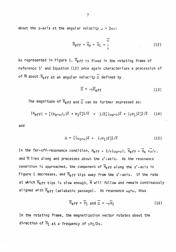
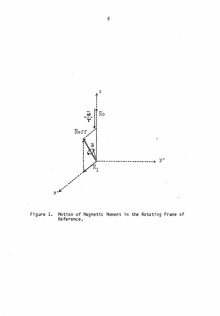
about the z-axis at the angular velocity w = 2nv:
w Heff = Ho + H1 + -
y { 12)
As represented in Figure 1, Heff is fixed in the rotating frame of
reference S' and Equation {12) once again characterizes a precession of
of "H about He ff at an angular velocity Q defined by
Q = -yHef f {13)
The magnitude of "'Reff and Q can be further expressed as:
IHeffl = [{H0-w/y)2 + H12]1/2 = 1/2[{w0-w)2 + (yH1)2]1/2 {14)
and
Q = [(w0-w)2 + {yH1)2]1/2 {15)
In the far-off-resonance condition, Heff = l/y{w0-w), Heff = H0 +w/y,
and 1-i lies along and precesses about the z'-axis. As the resonance
condition is approached, the component of Heff along the z'-axis in
Figure 1 decreases, and "'Reff tips away from the z'-axis. If the rate
at which Heff tips is slow enough. M will follow and remain continuously
aligned with Heff {adiabatic passage). At resonance w0=w, thus
In the rotating frame, the magnetization vector rotates about the
direction of 111 at a frequency of yH1/2n.
{16)
Q v
---·--------------------~ y I
Figure 1. Motion of Magnetic Moment in the Rotating Frame of Reference.

9
2. Fourier Transform NMR
NMR experiments can be carried out either by sweeping the
radio frequency (RF) applied to a sample in a fixed magnetic field or,
alternatively, slowly sweeping the field with a fixed RF. Both
techniques are referred to as continuous wave (CW) NMR.
·Another method of observation. based on pulsed NMR. suggested by
Bloch et~· (49,50) and put into practice initially by Hahn (51). makes
use of short bursts. or pulses. of RF power at a descrete frequency
known as the carrier frequency F. A short pulse of RF irradiation oft
seconds duration is equivalent to the simultaneous excitation of all the
frequencies in the range F±t-1. Hence, by using a very short pulse. it
is possible to excite all the magnetic nuclei of a given isotopic type
in a molecule simultaneously.
In the pulsed NMR experiment, a RF pulse tips the magnetization
away from the z-axis; the magnitude of Mxy. known as the free induction
signal. starts to decay after the removal of the short pulse and is
monitored along a fixed axis in the rotating frame (the y'-axis). The
monitored signal as a function of time is known as the free induction
decay (FID) or the time domain spectrum. The FID can be interconverted
with the frequency domain spectra (those obtained in the CW NMR
experiments) by means of the mathematical process of Fourier
transfonnati on.
The relationship between the time and frequency domains can be
expressed in the fonn

10
+co F(w) == J f(t) exp (-iwt)dt ( 17)
-co
and the inverse relationship
+co f(t) = f F(w) exp (iwt)dw ( 18)
-a:i
where F(w) is a function of frequency and f(t) is the corresponding
function of time. Thus pulse NMR with Fourier transfonnation is
referred to as Fourier transfonn (FT) NMR.
Since the sweeping rates of the CW NMR are limited due to
relaxation processes {section II.A.3), the total experimental time of FT
NMR, which simultaneously excites all the nuclei of interest. can be
substantially shortened in cornpari son. Therefore, FT technique enables
NMR studies of systems of inherently poor sensitivity, many repeated
pulses being applied.
A few of the techniques and terminologies of the pulsed FT NMR
which will be referred to in this dissertation are discussed in the
following.
Accumulation of Spectra
One of the simplest ways of overcoming sensitivity problems in
spectroscopy is to record several spectra from a sample and then simply
add them together. NMR signals will add coherently, whereas the noise,
being random, will only add as the square root of the number of spectra
accumulated. This leads to an overall improvement in signal-to-noise

11
ratio (S/N) by the square root of the number of spectra accumulated.
For example, adding 100 spectra will lead to an increase in
signal-to-noise ratio of 10:1. The principal drawback of this technique
arises from the time taken to obtain an individual spectrum or scan. It
is here that FT NMR makes a great contribution.
Pulse Duration and Flip Angle
As discussed in section II.A.l, in the rotating frame, at
resonance, the magnetization vector rotates about the RF H1 at a
frequency of yH1/2n (Equation (16)). If Hi is chosen to be along the
x'-axis, then a RF pulse of duration of tp will flip the magnetization
(in the y'z plane) away from the z-axis by an angle, the flip angle,
(19)
For example, a pulse duration of n/2yH1 will flip the magnetization by
90° and align it along the y'-axis. The pulse is referred to as a 90°
pul se.
Spin Locking
Immediately after a go 0 pulse (along the x'-axis). the RF pulse may
be phase shifted by go 0 and applied along the y'-axis. In the rotating
f~ame, the magnetization is then aligned along and precessing about the
Reff (Heff = H1) at a frequency of yH1/2n. This keeps the magnetization
vector from dephasing due to magnetic field inhomogeneity and the
process is referred to as spin locking.

12
Digital Resolution and Acquisition Time
In carrying out the Fourier tl"ansforn1ation, half of the available
data points are lost since the Fourier transfonn contains both real and
imaginary components and only the real component is used to generate the
spectrum (Equation (17)). Hence, if the original FID were accumulated
with N data points, the transformed frequency domain spectrum will
contain 0.5N data points. If the recorded spectral width in Hz is c.. then the digital resolution or accuracy of the spectrum in Hz will be
26 R =
N
Also. from the sampling theorem (Nyquist theorem), acquisition of a
(20)
frequency spectrum 6 in width requires a minimum sampling rate of 26
points per second. Thus the free induct"ion decay has to be acquired in
a time At (data acquisition time) ·~vhich fulfills the condition
26At = N (21)
Combining Equations (20) and (21). one obtains an accuracy in Hz of
26 1 R = = (22)
N At
i.e., the more the data points of the FID or the longer the acquisition
time, the better defined is the spectrum and the higher is the
resolution.

13
Signal Weighting, Digital Filtering and Zero Filling
It is possible to alter the FID sign.~ls mathematica"!ly to improve
either the resolution or the sensitivity (S/N) in the transformed
spectrum. For example, multiplication of the FID by a simple
exponential can reduce noise at the expense of some artificial
broadening of the 1 ines (resolution). Tile signai 1r1eighting process
which reduces noise and improves S/N is referred to as digital
filtering.
Another way to beneficially alter the FID signals is to supply
additional zeros to the digitized FID signal to create apparently 1 onger
signals. The process, known as the zero filling, does not improve the
resolution but it does improve spectral appearance and definition.
The Digitization Process and Dynamic Rar.ge
In FT NMR, every data point of the FIO is digitized by an
analog-to-digital converter (ADC) before being stored in a computer
memory. If the largest signai, of intensity H5 , is adjusted so as to
fill the whols conversion range. then fer an ADC of d bits, the limit
of the relative converter accuracy wi 11 be Hs/2d. This 1 imi t
characterizes the so-cal 1 ed Ii resolution of the converter" or the
11 numericai resolution". The smallest signal which can be recorded will
have an intensity Hw such that
(23)
This ratio is called the dynamic range of the spectrum.
14
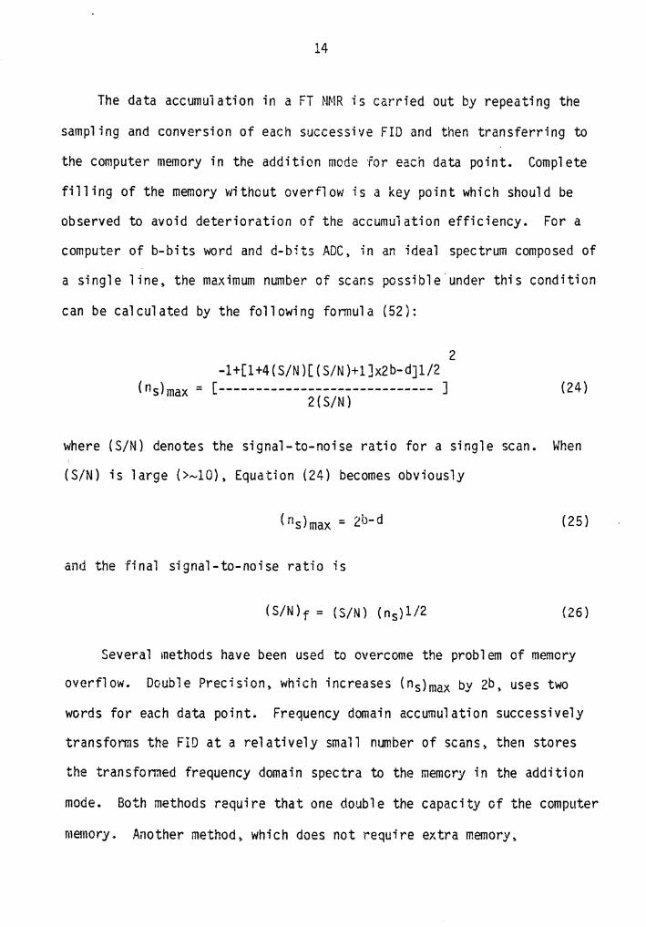
The data accumui ation in a FT NMR is carried out by repeating the
sampling and conversion of each successive FID and then transferring to
the computer memory in the addition mode for each data point. Cornpl ete
filling of the memory without overflow is a key point which should be
observed to avoid deterioration of the accumulation efficiency. For a
computer of b-bits word and d-bits ADC, in an ideal spectrum composed of
a single line, the maximum number of scans possible.under this condition
can be calculated by the following formula (52):
2 -1+[1+4(S/N)[(S/N)+l]x2b-d]l/2
(ns)max = [----------------------------- J (24) 2(S/N)
where (S/N) denotes the signal-to-noise ratio for a single scan. When
(S/N) is large {>~10), Equation (24) becomes obviously
(25)
and the final signal-to-noise ratio is
(S/N)f = (S/N) (ns)l/2 (26)
Several methods have been used to overcome the problem of memory
overflow. Double Precision, which increases (n 5 )max by 2b, uses two
words for each data point. Frequency domain accumulation successively
transfonns the FID at a relatively small number of scans, then stores
the transfonned frequency domain spectra to the memory in the addition
mode. Both methods require that one double the capacity of the computer
memory. Another method. which does not require extra memory.

15
progressively reduces the ADC bits at the expense of dynamic range.
3. Relaxation Processes
T1, T2 and Lineshapes
Following any perturbation which disturbs the magnetic equilibrium
of a spin system, for example. a 90° pulse which 1 eaves ~y 1 =Mo and
Mx'=~lz=O, the system returns to equilibrium via at least two relaxation
processes. The characteristic times T1 and T2 were initially used by
Block to describe these with the decay of magnetization assumed to
be a first-order process in each case ( 49, 50). (This assumption turns
out to be true for liquids but not for solids, at least as far as T2 is
concerned (53)). The longitudinal or spin-lattice relaxation time Ti,
describes the repolarization of the magnetization along the z-axis as it
comes to equilibrium through energy change with its surroundings
( 11 the lattice"). The transverse or spin-spin relaxation time T2,
describes the dephasing of the mangetization in the xy plane without
change of the total energy of the spin system. The Bloch equations can
be written in the rotating frame as (47):
dMx• Mx I
= -(w-wo) My• -dt T2
(27)
dMy• My I
= (w-w0 )Mx' + yH1Mz -dt T2
(28)
dMz' Mo-Mz l
= -yHJ.My I + dt T1
(29)

16
After the removal of the RF pulse (which was chosen to be along the
x'-axis), the system returns to equilibrium according to the following
formulae:
dM I Mx I x - - (30) dt T2
dM I My I 'Y - - (31)
dt T2
dM I (Mz'-Mo) z - - -------- (32)
dt T1
The solutions of the Block equations give a Lorentzian line, centered at
Vo, with bandwidth at half intensity given by
1 vl/2 = ( 33)
T 'lt•2
The observed bandwidth usually includes a contribution due to field
inhomogeneity 6H0
+ ---- (34) 2'Jt
or
1 (35)

17
wl1ere T 2* is defined as
, 1 yLH0 J.
= + ( 36) T2* T2 2
The Lorentzian lineshape and Equations 33-36 are indeed observed
for the non-viscous liquids. Most rigid solids, however, exhibit more
complex Gaussian lineshapes, where the transverse magnetization decays
exponentially as t2 (53).
Relaxation Mechani srns
In NMR (the probability of spontaneous emission being negligible)
restoration of the equilibrium populations following a perturbation
occurs relatively slowly and through stimulated emission. In general •
any mechanism which gives rise to fluctuating magnetic fields at a
nucleus is a possible relaxation mechanism. In this regard, a number of
interactions have been found to be important. These mechanisms are:
1. Magnetic dipole-dipole interaction.
2. Electric quadrupolar interaction.
3. Chemical shift anisotropy interaction. 4. Seal ar-coupl ing interaction.
5. Spin-rotation interaction.
6. Paramagnetic interaction, which includes both a dipole-dipole and a scalar-coupling interactions between an unpaired electron and a nucleus.
In fact, one or several of the mechanisms may be encountered in a
sample. An experimental relaxation rate is usually considered as a
summation of the specific rates of all the relevant mechanisms, m.

18
involved.
1 1 R· l = ------- = {i=l,2) (37)
Ti (obs)
Correlation Time ("c) and its Relationships to the Relaxation Times
Since in a rotating frame. the magnetization M appears to be
stationary, obviously only the fluctuating magnetic fields which are
fixed in the rotating_ frame can perturb M and contribute to the
relaxations. Therefore, all the possible relaxation mechanisms may be
affected by molecular motion (or other equivalent processes, such as
chemical exchange). In addition, the strength of any particular
interaction along with the magnitude and frequency of the molecular
motion, determines the relaxation rates.
The relaxation rates of each mechanism can be written as (13):
1 (38)
where Ee represents the strength of the specific relaxation interaction
and fim("c) is determined by the molecular motion. An example of
f imhc) or the effect of molecular motion on the relaxation rates may be
obtained by comparing Ti and Tz.
Spin-lattice relaxation processes which tend to bring the
magnetization vector back toward its equi1 ibrium state aligning along
the z-axis are, inevitably, accompanied by a decrease in Mx and My and
so also contribute to T2. However, Tz is always found to be equal to or
smaller than Ti, i.e., additional processes exist which can dephase the

19
spins without exchanging energy with the lattice. In fact, Tl and T2
are governed by the same mechanisms and Ee for both Tl and T2 of any
relaxation mechanism is the same. Thus, it is the function fim{~c}. or
the effect of molecular motion, which differentiates the two relaxation
times. It can be shown (13) that for a microscopic fluctuating field h,
hx' and hy' are effective in both Tl and T2 relaxation processes, while
hz' interacts effectively only with Mx' and My'. i.e., it is only
effective for the T2 relaxation processes. Since a static component of
1i in the z' direction of the rotating frame is equivalent to a static
component in the z direction of the laboratory frame, slow and low
frequency processes affect only T2. On the other hand, high frequency
processes (at resonance frequency or higher) affect both T1 and T2.
Thus, in non-viscous liquids, in which high frequency processes
dominate, one usually finds that T1=T2. while in rigid sol ids, in \"hi ch
high frequency processes are extremely limited~ T2<<T1 is the case.
In the function f;m(~c), ~c is the molecular correlation time,
which denotes the 11 average" time for a molecule in a state of motion or
in other words. it characterizes the rate ,3t which the 1 ocal fluctuating
field n loses memory of a previous value. For example, it can be
expressed as the average time between molecular collisions for a small
molecule in a liquid, or the average time required to effect a rotation
of 1 radian for large molecules.
In the simplest case of a single correlation time, the correlation
function can be written as
K{~) = C · exp{-l~l~c) (39)

20
where C is a constant. (By defiwition, K(·d= jY(t) ·Y*(t+·d j, \.Jhere
Y* is the complex conjugate of Y, and Y can describe a fluctuating field
or be an equation of motion).
Furthermore, a correlation time can be Fourier transformed into a
spectra density function
+co J(w) = J k(")exp(iwt)d~ (40)
-co
For example, if a molecule persists in some state of motion fer a time -12
of 10 sec. ("c), then according to Equations (39) and (40), its motion will have frequency components from 0 to io12 Hz.
The spectra density function J(w} gives the intensity or
probability of the,molecular motions at any specific frequency. Thus,
J(o) which is related to T2, and J(wo) as well as J(2w0 ) which is
related to T1 and T2 may be obtained from the molecular correlation time
"c, or vice versa. The value of ~c and molecular dynamic information can
be estimated from Tl and T2 (54-56) and other relaxation parameters.
(The contribution to T1 and T2 from J(2wo) arises from a sort of molecular Doppler effect (13).)
In many organic systems, including the samples studied in this
dissertation, the nuclear dipole-dipole interaction is the dominant
relaxation mechanism. (Barring the presence of paramagnetic impurities,
since the electron magnetic moment is much larger than the nuclear
moments, the dipole-dipole effect results in Tl (observed) ~Tl
(paramagnetic)). An exampie of TlDD and T200 as a function of the
correlation time between two identical spin 1/2 muclei undergoing
isotropic reorientation at various H0 is given in Figure 2 (57).

' "' 109
21
-:-. (s)
Figure 2. Behaviour of the Dipolar Spin-Lattice Ti DD and Spin-Spi~ T2 OD Relaxation Times as a Function of the Correlation Times •c for Interaction Between two Identical Spin 1/2 Nuclei Undergoing Isotropic Reorientation. The
wher~
functions 91 and 92 represent t~e parts of the relaxation rates T1-l and T2-I which reflect the dependency on •c and are independent of the distance separating the nuclei. (57)
1 •c 4•c = kgl with 91 = + -------- (41) -------T1 DD l+w2•c2 1+4w2•c2
1 1 s.c 2•c = kg2 if/i th 92 - - (3·tc + ------- + --------) (42)
T2 DD 2 l+w2•c2 1+4w2•c2
3µ02 1i2y4 3 1i2y4 k = {SI) or k ·- (CGS)
1601t2 ,.. 10 rrs6 rrs0

22
From Figure 2, it can be seen that the spin-lattice relaxation is
the most effective when the molecular correlation frequency (l/•c) is
equal to the nuclear precession frequency ( v0 ), and the spin-spin
relaxation is the most effecti~e when •c is the longest. Also, from
Equations (41) and (42), it is obvious that in the case of a short •c
( i . e. , w• c « 1 ) ,
1 T100 = T20D = (43)
4. Relaxation Time Measurements (13,15,45)
The basic versions of the most used methods for relaxation
time measurements employing pulsed FT NMR are reviewed below:
T1 Measurements (1) Inversion Recovery Method
This method uses the following sequence: (180°-.-90°-At-t)n
where • is a variable delay, At is a data acquisition time and tis a
recovery time (or pulse delay time) chosen as (At+th5T1. In this
method, line intensity from the solution of the Block equation (Equation
(32)) is expressed as
M(.) = Mo[l-2exp(-./T1)J (44)
where Mo practically can be achieved when •=5T1. When an estimate of
the Tl value can be made, a ca. 10. experiment spanning a range between
0.3 Tl and 2Tl as well as a long •{) 5Tl) is carried out and the value

23
of Ti is obtained from the slope of the plot of ln(M0 -Mh)/2M0 ) versus
.... This method is considered to be the most reliable. Hm~ever, a
recovery time of 5T1 makes this method time consuming and infeasible for
the systems with long Ti values.
(2) Saturation Recovery Method
The sequence for this method is (90°-HSP--i--90°-At-HSP)n.
Immediately after the first 90° pulse, Mz=O, a homospoil pulse (HSP)
further destroys the transverse magnetization. Following a variable
delay time of-.., M(.-)=Mzh}, is sampled by means of a second 90° pulse.
The corresponding line intensity for this method is expressed as
(45)
T1 is obtained from the slope of the plot of ln(Mo-Mh)/M0 ) versus
....
(3) Progressive Saturation Method
This method is a modified version of the saturation recovery
method and is 1 imited to the case Tp>T2 (or Tp>T2*). The sequence for
this method is: (90°-At--i-ln. The first five to ten scans are deleted
to reach a spin-system steady state. The corresponding line intensity
for this method is
. -(At+•) M(~) = M0[1-exp{-------)]
T1 J..
(46)
24
Again, T1 is obtained from the slope of the plot of ln(Mo-M(·d/M0 )
versus• (or At+,).
T2 Measurements
T2 measurements are much more demanding than T1 experiments,
especially in the case of short T2 (i.e •• rigid sol ids). Methods of
accurate T2 measurements have been achieved based on echo formation.
such as the Carr-Purcell method and the Meiboom-Gill modification of the
Carr-Purcell method (CPMG sequence).
No T2 experiment was carried out in the present study, ho1t1ever,
T2* 1 s were estimated from lineshapes and FIDs. Thus, no further
discussion w·i11 be provided on this topic.
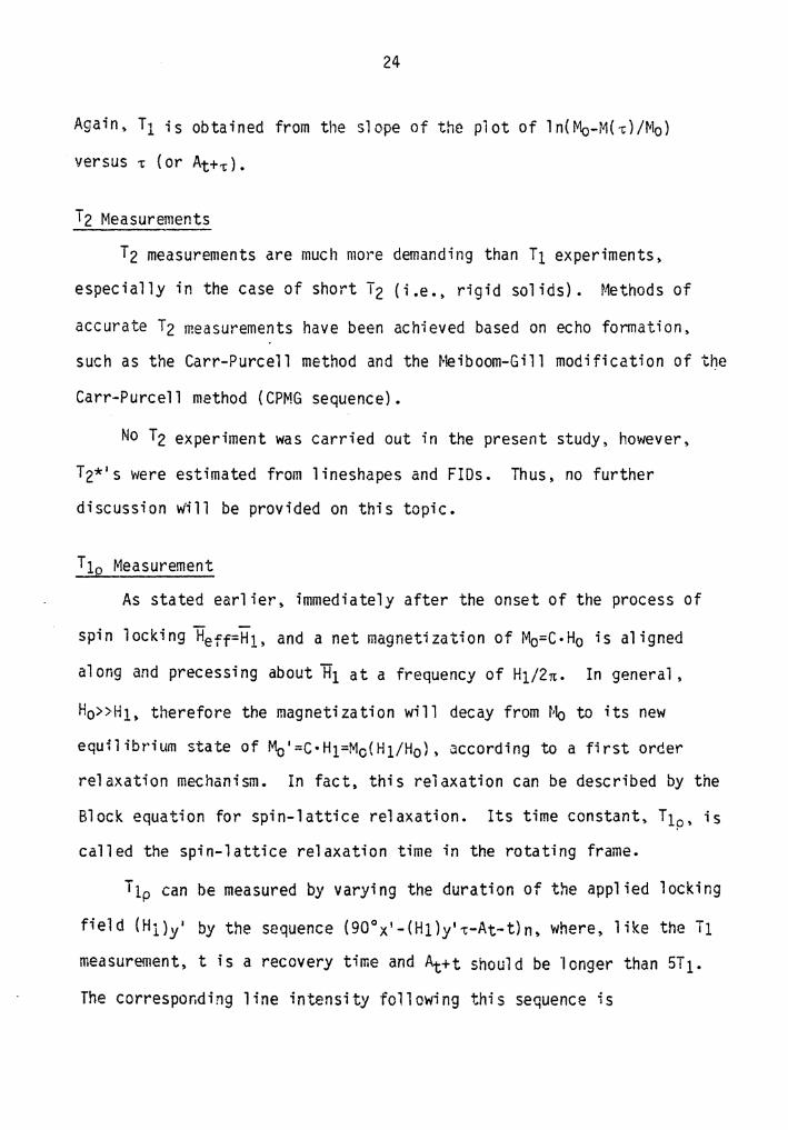
T lo Measurement
As stated earlier, immediately after the onset of the process of
spin locking Heff=H1. and a net magnetization of M0 =C·Ho is aligned
along and precessing about Hi at a frequency of Hi/2n. In general.
Ho»H1. therefore the magnetization will decay from Mo to its new
equilibrium state of Mo'=C·H1=Mc(H1/H0 ), according to a first order
relaxation mechanism. In fact, this relaxation can be described by the
Block equation for spin-lattice relaxation. Its time constant, Tip• is
called the spin-lattice relaxation time in the rotating frame.
T1p can be measured by varying the duration of the applied locking
field (H1)y 1 by the sequence (90°x 1 -(H1)y'•-At-t)n. where, like the Tl
measurement, t is a recovery time and At+t should be ·1anger than 5T1.
The corresponding line intensity following this sequence is
25
and the value of T1p is obtained from the slope of the plot of
ln(M{~)/M0 ) versus ~-
(47)
The T1p process is most effective when the molecular correlation
frequency is equal to yH1/2~ (1-lOOKHz). Thus, the T1p experiment is a
powerful tool for probing the low frequency processes in this range.
5. The NMR Parameters
Besides T1, T2. lineshapes and T1p• four NMR parameters, which are important in the study of molecular structure and dynamics are discussed
below.
Chemical Shi ft. o Deriving from the magnetic effect of the surrounding electrons, a
1 II •II • f. 1 d "Tt· Tr A - A nuc eus l exper1ences a 1e ni = H0 -ciHo. where 0 ; is the shielding
tensor (of second rank) which characterizes the spatial electronic
distribution around the nucleus.
In general, the electronic shielding is anisotropic. However, due
to the existence of fast and isotropic molecular motion, an averaged
isotropic value. a;, is detected by NMR experiments on liquids. This
value represents the mean of the three principal components of the A
tensor ((l/3)trcri) and is called the shielding (or screening) constant.
The resonance frequency of the nucleus 11 ·i 11 is, according to
Equation (6):
26
y Vi = --(Ho-criHo)
2n
y = --(1-a;)Ho
2n (48)
The positions of the various signals are usuaily compared with the
resonance of a standard substance (Tetramethyl Silane for 13c and lH),
and the chemical shift is defined as
Hi-Href vi-v ref Oi = a ref - O'i = ------- = -------
Ho VQ
(49)
o; is a dimensionless parameter which does not depend on the strength of
H0 (or v0 ) and is expressed in units of 10-6 (ppm).
Spin-Spin Coupling Constants
In addition to the electronic diamagnetic effect, a nucleus 11 i 11 may
experience the fields associated with the presence of neighboring spins.
Theoretically, two mechanisms of interaction between the nuclear
magnetic dipoles are liable to intervene: a direct through-space
interaction depending on the internuclear distances, and an indirect one
transmitted through the bonding electrons. Both interactions are
independent of the strength of H0 •
(1) Direct (Dipolar) Coupling Constant, D
The direct spin-spin coupling interaction is described by a
traceless second rank tensor ~. !n the case of two isolated spin 1/2
nuclei 11 i 11 and 11 j 11 , the direct coupling constant is given by

27
h {3cos2e;j-l) Dij = - 4-it- YiYj ------------r;j3
(in Hz) (50)
where 0ij is the angle between the applied field Ho and the internuclear
distance ~ij· Doublet resonance lines centered at YiHo/2it (or
YjHo/2it) separated by l2D;j I are expected for the spectrum of nucleus i
(or j) •
In an ensemble, Equation (50) can be written as
-h <3cos2e-1> - - -- YiYj 4it r· ·3 lJ
(51)
where<> denotes a value averaged over all magnetic {i,j) dipoles. The
magnitude of D;j (for 13C-1H or lH-lH) is in the order of 104-105 Hz.
Therefore:
(i) In liquids, •c << 1/2 D;j. isotropic motions result in
<3cos2e-l>=O and Dij is nullified.
(ii) In solids, •c > 1/2 Dij. the orientation term of Equation (51)
can not be averaged to a single value, and numerous dipolar couplings
produce the very broad lines observed.
(iii} In highly oriented mesophases. D;j's have been successfully
measured and fonn the basis for molecular geometry studies (58).
(2) Indirect (Spin} Coupling Constant, J
The indirect spin-spin coupling interaction is al so described by a A second rank tensor J. The interaction of the J-coupling is much weaker
than the D-coupl ing (for 13c and lH, by ca. 2-4 powers of ten). Thus in

28
solids, the J-coupling is obscured by the direct 0-couplings. In A liquids, due to the existence of fast and isotropic motions, J is
A reduced to a constant, (l/3)trJ, whose magnitude is the mean of tile A three principal components of the J tensor.
For two spin 1/2 nuclei, i and j. the indirect coupling is given
by
fl 1 A J;J· = -- r;y.; (-trJ;J·)
2n J 3 ( 52)
Resonance lines of both i and j are split to form a doublet, separated
by IJ;jl.
The signal multiplicity arising from the J-couplings facilitates
the elucidation of the NMR spectra.
Resonance Line Intensity
Integrated areas under each NMR signal for the spectra obtained
under certain appropriate conditions can be directly proportional to the
number of nuclei in a particular environment. This provides for a
quantitative analysis of the NMR spectra.
Nuclear Overhauser Factor •.....21
As stated earlier, two nuclei, i and j, when close enough, can
interact through space in a dipole-dipole mechanism. When one of these
nuclei (j) is irradiated (i.e., saturated by means of a complementary RF
field Hz, or decoupled}, it can lead to a modification of the energy
level populations of the second (i) and results in a modification of the
intensity of the r'esonance 1 ine of the nucleus i. This phencmenon,

29
known as the nuclear Overhauser effect {NOE), like T1 and T2, depends on
the strength of H0 and on molecular mobility.
The NOE is characterized by an enhancement factor
I;-Iio T) =
where I; and Iio are the resonance line intensities of nucleus i
obtained with and without irradiating the nucleus j.
(53)
Besides the advantage of sensitivity enhancement by NOE in many
cases (when n>o), the nuclear Overhauser factor, TJ, can also be used to
determine the contribution of the dipole-dipole interactions to the
total relaxation process and to probe the molecular mobility when 'tc ; 5
in the neighborhood of l/v0 (i.e., viscous liquids or non-rigid solids)
( 59) •
8. Introduction to Solid State NMR
As discussed briefly in the introduction and the last section, the
anisotropic nature of most solid samples results in broadline NMR
spectra. However, with recent advancements in NMR technology, namely
the high speed magic angle spinning and multiple pulse decoupling
techniques, high resolution "liquidlike" spectra of solid samples are
attainable for all 118 NMR-active isotopes in the periodic table (60).
Nonetheless, the most easily achieved and well developed experiments
have been among those spin 1/2 nuclei which have weak (homonuclear)
mutual coupling either by virtue of low natural abundance or small
magnetic moments (e.g., 13c, 31p, 29si, 15N, 195Pt, 199Hg). Therefore,

30
besides the resolution prob 1 em. sensi tiv'ity is another obstacle for the
studies of those nuclei. The sensitivity problem arises not only from
the weak macroscopic magnetic moments, but also from long spin-lattice
relaxation times in solids. concomitant with the weak homonuclear
dipolar interactions and aggravated by the lack of high frequency
molecular reorientations in rigid solids.
The following two sections will revie\I/ the resolution and
sensitivity problems of solid state NMR and their solutions. A general
treatment will be given, although the focus will be on 13c and other
spin 1/2 nuclei having weak mutual coupling.
C. The Resolution Problem: Sources of Line-Broadening and Methods for their Removal
In addition to electron shielding. direct dipolar interaction and
indirect electron-coupled interaction as discussed in the previous
section, another main source of line-broadening in solid state NMR
spectra is electric quadrupolar interaction. The electric quadrupolar
interaction has already been mentioned as a possible relaxation
·mechanism and is frequently encountered in heteronuclei NMR because at
least 87 of the NMR active isotopes possess a spin value I>l/2 and,
thus. have a quadrupole moment Q.
These four interactions just mentioned along with the naturai
lineshape (or lifetime-broadening. which may be regarded as an effect of
the uncertainty principle, i.e., t,E·t;t=(liv1;2)t,~h and v112=l/7tT2)
determine the pattern of a solid state NMR spectrum, as shown in Figure
3 (60).

Dipolar Shielding
(e)
® ®
and
(c~{'.:~:~~'.;j{;~
Quadrupolar J Coupling Lifetime
(I)
(g)
® :~ .
(h) J.. ® ~
Figure 3. NMR Powder Patterns of Nuclei. The following interactions are present: 1) dipolar coupling between two isolated spins (a). dipolar coupling between three isolated spins (b). and dipolar coupling among many spins (c); 2) shielding anisotropy. nonsymmetric (d) and axially symmetric (e) patterns; 3) quadrupolar splitting. the central 1/2-1/2 transition for a spin 3/2 system (f); 4) J coupling. same form as two-spin dipolar pattern (g); and 5) lifetime broadening (h). The total spectrum of nuclei experiencing all of the above interactions will be a convolution ( ) of all of the above spectra. (60)
w __,

32
More precisely, the NMR spectrum of a nucleus may be described by a
series of interaction Hamiltonians, including nuclear spin interactions
with both the external fields (H0 , Hi) and internal fields,
(54)
where
( 55)
Ho and Hi are the Zeeman interactions with the external fields H0 and
111, respectively. Hint consists of the four interactions which were
referred to as the main sources of line-broadening observed in the solid
state NMR spectra.
(56)
The various interactions may be written as:
electron shielding (57)
- A direct dipolar interaction Hct = 2~ I;-D;J··IJ· , i<j
(58)
indirect electron -coupled -inte~action (59)
electric quadrupolar interaction eQ; A -
Hq = 'i' ---------- T; ·Vi ·Ii .(60) 6 i 6I;(2I;-1)
In Equation (60), ~i is the electric field gradient tensor at nucleus i.
33
A A In Equations (57-60), among the four interaction tensors. D and V are
A A traceless. whi 1 e a and J are not restricted. Hov1ever. two traceless
tensors, ~* and ~* can be obtained by subtracting the constant . . f A A 1 sotrop1 c trace rom a and J.
A
A A A A a* = a - u1 where a = ( 1 /3) tra
A A A A J* = J - Jl where J = (l/3)trJ
and 1 is the unit tensor.
Equations (57) and (59) can be rewritten as:
( 61)
(62)
(63)
(64)
In the instance of fast and isotropic molecular reorientations.
the time-averaged Hamiltonians due to the four traceless interaction
tensors drop out of the model • Thus.
H s = flrr; ·a; -Ho (65) 1
Hd = 0 (66)
Hj = h'i' i; .J;; .TJ· 1<j ..
(67)
Hq = 0 (68)

34
These terms then represent what 1 s obser-ved in the NMR spectra of
non-viscous liquids.
Theoretically, for solid samples. one can see how an alternative
approach would eliminate all the anisotropic interactions due to the
internal fields (61,62); this becomes possible through magic angle
spinning (MAS), an angle of about 54.7°. Because of experimental
reasons. the direct dipolar interaction (Hd) is usually removed by
the technique of decoupling. which also removes both the isotropic and
anisotropic parts of the other interaction involving two nuclear
magnetic dipoles (i.e. Hj). Both methods are discussed below in more
details.
1. Magic Angle Spinning
The magic angle is 54° 44' 811 = arc cos (1/3)1/2, and magic
angle spinning is the technique of rotating the whole solid specimen
(within a rotor} uniformly about an axis inclined to H0 at the magic
angle. The power of the MAS can be partially realized by inspection of
Equation (50} for the direct coupling constant. Either the isotropic
average <cos2e;j>=l/3 or the magic angle coseij = (1/3)1/2 can lead to
<3cos2e;j-1>=0 and, thus. D;j=O. In fact, it is the angle ~. between
the mechanical spinning axis and "Ff0 adjusted to be equal to the magic
angle, irrespective of the Gij's. Nonetheless. under spinning
conditions, the time-independent term of the time-averaged Gij (the
time-dependent terms generate spinning sidebands) will go to zero
because. in spite of its initial value, it contains a multiplier
( 3cos2~ -1) .

35
Spinning Rate
In order to remove the anisotropic ·interactions effectively by M.l\S,
it is necessary that the rotation pericd for the sample be short
compared to the spin-spin relaxation time or dephasing time, T2. of the
individual spins. In other words, the spinning rate (Hz) has to be
large compared to the linewidths {Hz) associated with the spins (39).
The ultimate spinning rate of a gas-driven rotor is governed by the
linear velocity of its periphery. It can not exceed the speed of sound
(63). For example, a 1 cm diameter rotor has a maximum theoretical
rotation rate of 10.5KHz in dry air. Although, using a selective dr·iver
gas, helium, for example, in which the speed of sound is 2.7 times
greater than in air, one might achieve a maximum theoretical spinning
rate which would be 2.7 times faster. However, this upper limit is
usually impractical as most materials used to confine samples
disintegrate due to centrifugal forces at such velocities (39).
In general. MAS is carried out at a rate in the range of 3-5 KHz.
This is not fast enough to remove the pre ten-proton and carbon-proton
dipolar interactions (in the range of 10-40 KHz), although it has been,
indeed, successful in removing the di polar interactions of some nuclei
of small magnetogyric ratio (61,62,64). MAS is also able to remove the
anisotropic part of the indirect electron-coupled interaction {65,66) as
well as the (first order) electric quadrupolar interaction (67}.
However, since in solid state carbon-13 NMR, MAS is aimed at removing
the chemical shift anisotropy (CSA) (ca. 1.8-3 KHz, for aromatic and
carbonyl carbons at an external field H0 of 1.4 Tesla), only the effects

36
of MAS on the CSA interaction are reviewed below.
Removal of the Chemical Shift Anisotrcpy by Magic Angle Spinning A Since any antisymmetric components of the shielding tensor a. have
negligible effects on the spectrum (68), the cl1emical shift of a nucleus
i with principal shielding elements ail. a;2. cr;3 and with direction A A
cosines between the principal axes of ai and Ho. Ail. Ai2. Ai3 is given
by (61,62)
2 2 2 0 izz = Ail 0 il + Ai2 °i2 + Ai3 cr;3 ( 69)
If the solid sample in which i is resident. is rotated at angular
velocity wr about an axis inclined to Ho at an angle~ and at angles ,A
~il. ~i2. ~i3 to the principal axes of a~ the direction cosines become
(K=l,2,3)
Aik = cos ~ cos @ik + sin ~ sin ~ik cos (wrt + Xik) (70)
where Xik is the azimuthal angle of the Kth principal axis (w.r.t. Ha) at t = O. From equation (70), one obtains:
2 2 2 kik2 = l/2[sin p + {3 cos ~-l)cos ~ik]
2 2 + l/2[sin p sin g;iik cos (wrt + X;k) + ( 71)
2 sin2p sin ~ik cos 2(wrt + Xik)]
2 2 where ~ik consists of a time-independent term (kik )0 and a
time-dependent term (Aik2)t, which is periodic with zero mean value and
will generate sp·inning sidebands if the spinning rate is insufficient.

37
2 2 2 Aik = {\ik )o + (~ik }t
Substituting Equation (72) into Equation (69) one obtains:
3 2 3 2 o i zz = ) ( :\ i k ) o i k + ) (Ai k ) o i k
K.=l 0 K.=l t
Equation (73) describes a spectrum of a resonance line according to
t (Aik2) o;k with spinning sidebands at multiples of wr. k=l 0
The intensity of the sidebands decreases as the spinning rate -1
(72)
(73)
increases. At a sufficient speed (wr>T2m). the time-averaged value of
(69). Therefore. time-average yields the observed chemical shift.
specifically
2 3 2 l/2(3cos ~-l)I cos ~ikoik
k=l
If ~ is the magic angle. Equation (74) reduces to
A <o;zz> = 1/3(0;1+0;2+0;3) = (l/3)troi = oi
(74)
(75)
A regardless of the initial orientation of the principal axes of a; with
respect to "H0 and to the spinning axis.

38
Besides yielding "liquid like" spectra by high speed MAS of solid
samples, the method may also be modified. MAS at insufficient rates
(69~70) as well as off-MAS (variable angle spinning} at high speed (39)
have been used to extract components of the shielding tensor and to
study molecular orientation.
2. Decoupling (32,68)
As stated above~ any interaction between two nuclear magnetic
dipoles, homonuclear or heteronuclear. can be eliminated by saturating
the Zeeman splitting of one of the nuclei with a complementary RF field
"A' 2.
Heteronuclear Oipolar Decoupling
Heteronuclear decoupling can be carried out by irradiating the
entire chemical shift range of the nucleus selected for decoupling
(broad-band decoupling}. Heteronucl ear proton broad-band decoupling has
become standard for.C-13 NMR of liquid samples in order to remove the
isotropic (scalar) indirect spin-spin interactions (J-couplings). In
solid state C-13 NMR, the same procedure can be used to eliminate both
the direct and indirect (isotropic and anisotropic) spin-spin
interactions. However, the RF power required to remove the 10-40 KHz
dipolar coupling is considerably greater than that for the 100-200 Hz
scalar coupling. For this reason~ removal of heteronuclear
spin-spin interactions by high power broad-band RF irradiation is
referred to as "Di polar Decoupl ing 11 (DD) (38).
In the case of 13c or other nuclei having low natural abundance

39
and/or a small magnetic moment. the homonuclear spin-spin interaction is
a negligible source of line-broadening relative to the heteronuclear
interactions with nuclei having high natural abundance and/or a large
magnetic moment. Furthermore, high speed MAS usually removes the weak
homonucl ear interactions to a 1 arge extent. Therefore, combining
dipolar decoupling with MAS, high resolution 11 liquid like" solid state
NMR can be achieved for 13c and some other nuclei having weak
macroscopic magnetic moments.
Dipolar Decoupling by Spin Locking (71)
In solid state C-13 NMR, proton dipolar decoupling is actually
achieved by a spin locking process. A spin-locked nucleus. where
individual dipoles precesses about Hi, resulting in an oscillatory
component along the z-axi s, is decoupled from other kinds of nuclei
provided the precessing or oscillating frequency (depends on H1} is
greater than the dipolar interaction expressed in hertz.
Homonuclear Decoupling
Homonuclear decoupling experiments, where the observed and
decoupled nuclei are of the same type, are more demanding. In solution
NMR, a time-sharing procedure has been developed to carry out
homonuclear scalar decoupling (72). In solid state NMR, homonuclear
decoupling has been achieved by a number of multiple-pulse sequences
(73-76), which alternately drive the nuclear magnetic dipoles along the
three orthogonal axes. This results in a time-averaged value of
<cos2e>=l/3 without saturating either the observed or "decoupled"

40
nuclei. These methods can el i;ninate the anisotropic direct and indirect
spin-spin couplings. (In fact, they can remove both the homonuclear and
heteronuclear couplings as well as the electric quadrupolar
interactions.) The indirect scalar couplings are preserved while the
chemical shifts are modified without averaging out the anisotropy.
Combining MAS with multiple-pulse decoupling, high resolution
11 1 iquid 1 ike 11 sol id state NMR can be achieved for proton and many other
n uc 1 e i ( 3 5, 77} •
3. Factors Affecting Resolution in the High Resolution Sol id State NMR
The Gaussian lineshapes observed in the broad-line solid state
NMR are mainly due to the direct nuclear dipol ar interactions (78}.
After the removal of these interactions and other sources of
line-broadening, the lineshapes of the high resolution 11 liquidlike 11
solid state NMR are observed to be Lorentzian (79). However, the
resolution of the 11 liquidlike 11 solid state NMR is generally not as good
as in the liquid case. Furthermore, unlike solution NMR, increasing the
magnetic field may not help because chemical shift anisotropy is
proportional to the strength of the applied field H0 •
Besides T2, which determines the natural bandwidth, major factors
affecting the ultimate resolution of the (DD-MAS) sol id state C-13 NMR
both in terms of technical 1 imitations and sample effects are reviev~ed
below (36,80). These factors are, of course, among the major factors
affecting the resolution of the high resolution solid state NMR of other
nuc1 ei as well (62).

41
Technical Limitations
(1) Imperfect Adjustment to the Magic Angle
Let us assume that a spinning axis was 0.5° off the magic angle.
This results in a residual CSA of 1% of the static value (61). However,
this can usually be reduced further by trial-and-error adjustment of the
angle.
(2) Insufficient Spinning Rate
In certain cases, especially at high external field strengths, as
discussed before, if the spinning rate is less than the CSA, a spectrum
is broken up into a complex profile of sidebands centered around each
isotropic shift. This leads to a loss in sensitivity, as well as
confusion in spectral assignments. Methods have been introduced to
overcome this problem and thus to enable spinning-sideband-free solid
state NMR spectra to be obtained in high field super conducting magnets,
either by recovering the isotropic shifts from the sidebands (81) or
using a phase-adjusted technique (82).
(3) Other possible technical limitations include rotor
instabilities, insufficient decoupling power and off-resonance proton
irradiation (80}.
Sample Effects
Even under ideal experimental conditions, static and/or dynamic
effects can limit resolution in certain solid samples. These effects
include:
(1) Solid State Effect
Some carbons having the same chemical shift in the liquid state are

42
discernable (split) in the solid state NMR, (e.g •• the two
non-substituted aromatic carbons of poly(phenylene oxide)) due to higher
degrees of molecular orientation.
(2) Chemical Shift Distributions
The heterogeneous nature of amorphous materials, such as glassy
polymers. may result in a distribution of isotropic chemical shifts for
a single carbon. This can contribute several ppm of broadening (38).
(3) Dynamic Effects
Ironically. interference between coherent motion introduced by
the line-narrowing techniques (e.g •• spin locking and sample rotation)
and molecular motion can combine to degrade the resolution gained by
these techniques (38,77,80,83).
(4) Another effect is the residual dipolar interaction between 13c
and nuclei having a large quadrupole moment (e.g •• 14N, 35cl). which may
broaden the C-13 spectra of solids when the interaction is too strong to
be eliminated by MAS and when T 11 s of the quadrupol ar nuc·1 ei are too
long to induce 11 sel f-decoupl ing 11 (84).
Although these effects complicate and broaden the high resolution
solid state C-13 spectra. they can also lead to new structural and
dynamic infonnation of the sample studied.
D. The Sensitivity Problem and Its Solution
In this section. the sensitivity problem and approaches to its
solution are reviewed for carbon-13, although the discussion applies
equally well to other spin 1/2 nuclei having weak mutual coupling.

43
For convenience of the treatment, the conventional symbolism S
and I are employed to express the nuclei of 13c and lH respectively.
The local magnetic field induced by the magnetic moment of a proton
is expressed as:
H ~ µz
hz = <1-3cos2e> (76) r3
where r can be either the homonuclear or heteronuclear distance. The
Zeeman splittings due to this local field on its neighboring nuclei are
expressed as:
YH ~ ~VHH = 2 DHH = -- lhzl
1t
YC ~ ~VCH = 2 DcH - -- lhzl
1t
1. General Considerations and Definitions
(77)
(78)
The sensitivity problem of the sol id state C-13 NMR can be
considered in three categories.
(1) Low Natural Abundance (1.1%) and a Small Magnetic Moment
(µc~l/4µH).
(2) Poor Resolution. As discussed in the last section, even with
all of the line-narrowing techniques available, NMR resolution in solids
is still not as good as in liquids. Therefore, in terms of peak height,
one must require a substantially greater number of accumulations in
order to achieve the same S/N for a solid sample compared to a liquid

44
sample having the same {integrated) resonance line intensity and the
same number of scans.
{3) Long 13c•s Spin-Lattice Relaxation Times. Due to the two
problems indicated above, in general. a great number of accumulations
are needed to achieve a solid state C-13 spectrum with reasonable S/N.
Thus. the experimental time becomes 1 imited by the rate at which carbon
magnetization can be reestablished along H0 by spin-lattice relaxation
process (e.g •• in a 90° pulse sequence, a pulse delay time of ca. 5T1
between two scans). This process for C-13 in solids is usually
ineffecient due to the small magnetic moment. lack of high frequency
molecular reorientations and inefficient spin diffusion.
The first problem listed above can be circumvented with isotope
enrichment. while the second is anticipated to be ameliorable as
line-narrowing techniques progress. However, cross polarization (CP)
techniques (85) have overcome the third problem thus making C-13 NMR
studies of natural abundance solids possible. Cross polarization is a
particularly effective version of a double resonance experiment in the
rotating frame (71,86); it uses the large proton magnetization to
polarize the 13c nuclei. The rest of this section will review the
principles and effects of the CP technique.
2. Spin-Lattice Relaxation in the Sol id State
Comparison of lH's and 13c's T1 's
Since the CP process uses proton magnetization to polarize the
13c n1Jclei. the proton's T1 1 s have to be shorter than 13C's T1 1 s in
order to make the process effective. Recalling Equation {38)

45
i Rim = = Ec2f;m(~c)
T;m
where Ee for protons and i3c nuclei are rr2/r3 and YIYS/r3,
respectively. if one assumes that iH-iH and 13c-iH dipole-dipole
interactions are the dominant spin-lattice relaxation mechanisms for
protons and i3c nuclei. respectively. As stated before. the spectra
density of motions at WI and 2wI are responsible for proton's Ti's; it
can also be shown that motions at ws and wI±ws (i.e. wI/4. 3wI/4 and
SwI/4} are responsible for i3cts Ti's (i3.43}. Therefore. molecular
motion is not a significant factor in that proton's Ti's are shorter
than i3c's Ti's. Further if one assumes that in a hydrocarbon compound,
in which every proton and every C-13 nucleus can be considered to have
about the same number of protons of about the same proximity in its
neighgorhood, (polyethylene is a good case}. then the proton's Ti is
expected to be i6 times shorter than i3c's Ti. However. in the
crystalline region of semi-crystalline polyethylene. 13c's Ti has been
found to be 200-iooo times longer than the proton's Ti (39). It is the
very effective mechanism of spin diffusion among protons which makes
proton's Ti's usually much shorter than what would be expected according to Equation (38}.
Spin Diffusion
Spin diffusion is a process of rapid simultaneous transitions
("flip-flop") of dipolar coupled nuclei having antiparallel m~ents.
without physical movement of the nucleus. when the coupled nuclei have

46
the "same" precession frequency (43).
Spin diffusion does not involve energy exchange with the lattice.
However, spin diffusion among protons does lead to all of the protons
exchanging energy with the lattice through preferred relaxation sites.
When the spin diffusion process becomes more effective than the most
effective spin-lattice relaxation process (the diffusion rate is roughly
equal to ~VHH), all the proton's Ti's observed will be the same. Even in
an inhomogeneous (microheterogeneous) material, spin diffusion usually
enables the rigid regions to relax faster with the lattice than would be
possible without the process; again, semi-crystalline polyethylene is an
example (39).
The CP process, indeed, utilizes the concept of spin diffusion by
employing a double resonance technique to enable the protons and 13C
nuclei to precess at the "same11 frequency in the rotating frame.
Another effect of the spin diffusion among protons is that the
fluctuating magnetic fields due to the "flip-flop11 process reduce 13C-1H
interaction from ~vcH to ~vcH(~vcH/~vHH) (43).
3. Relaxation in the Rotating Frame
This subject has been discussed before in the section on
relaxation time measurements. Since CP is a process of double resonance
in the rotating frame, Tip of the protons will be a factor in obtaining
reliable intensities in the CP spectra, as discussed later.
Another concept, the spin temperature, which· might provide an
insight into the relaxation in the rotating frame and ·other nuclear
relaxation processes, as well as to the CP process, is reviewed below.

47
Spin Temperature in Solids (43,44)
Equation (8) describing the equilibrium macroscopic magnetization
can be rewritten as
where C is the Curie constant)
N0 µ2 (I+l) c = = ---------------
31 3
and Equation (79) is known as the Curie's law. In Equation (79) TL
denotes the lattice temperature to distinguish it from the spin
temperature Ts. Obviously, in the equilibrium state
As discussed earlier, when a spin system is perturbed, in the
{79)
{80)
(81}
existence of effective spin diffusion, a thermal equilibrium inside the
nuclear spin system characterized by a uniform spin temperature Ts
can be achieved in a time much shorter than T1 (i.e., when Tl>> T2.
since t.vHH-1 - T200). The spin temperature of such an 11 internal
equii ibri um 11 system is given by
Ts = CHeff
kM * 0
{82}

48
Where Mo* is the internal equilibrium macroscopic magnetization.
Therefore. Ts can be significantly different from TL in these spin
systems before the completion of the spin-lattice relaxation process.
On the other hand, the spin-lattice relaxation process of these systems
can be regarded as a thermal process of cooling the spin systems to
reach thermal equilibrium with the lattice.
In the rotating frame, at the beginning of the spin locking
process. Heff = H1, ~~* = M0 and Equation (82) becomes
Ts = CHo = ----- • =
kM0 Ho Ho (83)
Note that H0 is usually much greater than H1. Therefore, relaxation in
the rotating frame is a "heating" process. which finally reaches Ts =TL
with a much small er macroscopic magnetization Mo( H1/Ho) in the rotating
frame.
4. Cross Polarization (85)
Many CP schemes are possible (85), but only the commonly used
single-contact spin lock version is revie\t/ed in the following.
Hartmann-Hahn Condition (86)
The Hartmann-Hahn matching condition for nuclear double resonance
in the rotating frame is the key to the success of the CP method. The
condition is achieved by simultaneously applying two resonant
alternating RF fields in the xy plane, Hu and His. to the respective I
and S spins such that

49
(Y1/2n)H1I = vI = vs = (YS/2n)H1s (84)
Thus, in the rotating frame, I spins are precessing about HiI and s
spins are precessing about 111s at the same frequency. Both spin systems
generate oscillatory components along the z-axis at the same frequency
regardless of the phase angle between HlI and His. This enables a
heteronuclear (IS) spin diffusion (39) between the I-spins and the
S-spins. The two spin systems usually can reach thermal equilibrium I S
such that Ts =Ts in a time much shorter than Tlr and Tls,
The period of time in which the "H1r and "His fields are
sim_ul taneously applied is referred to as the contact time (38).
Cross Polarization Procedure
One of the variety of experimental methods (85) for establishing
contact of I and S spin systems and then observing the S-spin
magnetization is represented by the following sequence:
(1) establish I-spin magnetization in H0 in a period of time of
ca. 5Tll.
(2) spin-lock I-spins along H1I and simulatneously apply His to
contact S and I spins with a Hartmann-Hahn match.
(3) turn-off His and record S-spin FID. Keep Hir on as a dipolar
decoupler until the completion of S-spin data acquisition.
(4) repeat steps (1) - (3).
A modification of this sequence (87) shifts "H11 by i00° every
other spin lock sequence. Thus the S-spin magnetization grows
alternately parallel or antiparallel to His, even though the His itself

50
retains the same phase. By alternately adding and subtracting the
S-spin FID, RF transients are subtracted out, while the S-spin FIDs are
coherently added. Therefore, artifacts, such as pulse breakthrough due
to long receiver recovery times can be minimized or eliminated. The
sequence and its modification described above are used as a standard
procedure in all the CP spectra of this dissertation.
Sensitivity Enhancement {85)
As discussed before, establishing the Hartman-Hahn condition allows
the I and S spin systems to reach an internal equilibrium in a time much
shorter than T1r and T1s. Assuming that (TlpI)-1 is neglible (i.e. T1pI approaches infinity) relative to the cross relaxation rate (IS spin
diffusion), the spin temperature of the internal equilibrium state will
be: T I s (85)
where e = Cs/Cr and cs and er are the Curie constants for the S-spins and I-spins, respectively.
The cross-polarized S spin magnetization can be calculated by
substituting Equation (84}, (85) and Heff=H1s for the s-spin into Equation (82).
Mo*S = (1-e) YI
M0S = (1-e) M0S rs
(86)
Since 1-E - 1.0 in most organic compounds and YH/rc - 4.0, then Mo*C
- 4M C 0 •
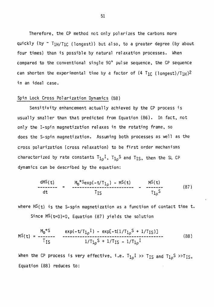
51
Therefore. the CP method not only polarizes the carbons more
quickly (by - T1H/T1c (longest)) but also, to a greater degree (by about
four times) than is possible by natural relaxation processes. When
compared to the conventional sin9le 90° pulse sequence, the CP sequence
can shorten the experimental time by a factor of (4 Tic ( 1 ongest) /TlH )2
in an ideal case.
Spin Lock Cross Polarization Dynamics (88)
Sensitivity enhancement actually achieved by the CP process is
usually smaller than that predicted from Equation (86). In fact, not
only the I-spin magnetization relaxes in the rotating frame, so
does the S-spin magnetization. Assuming both processes as well as the
cross polarization (cross relaxation) to be first order mechanisms
characterized by rate constants T1pI• T1pS and Trs. then the SL CP
dynamics can be described by the equation:
dMS( t) Mo*Sexp(-t/T1p) - MS(t) MS(t) -------- =
dt Trs (87)
where MS(t) is the S-spin magnetization as a function of contact time t.
Since MS(t=O)=O. Equation (87) yields the solution
MS(t) = M *S 0 exp(-t/T1pI} - exp[-t(l/T1pS + l/Trs)J
-----------------------------------------1/T lp s + 1/Trs - l/T1pI
(88)
When the CP process is very effective, i.e. T1pI >> Trs and T1ps >>Trs.
Equation (88) reduces to:

52
MS(t) = M0*S [exp(-t/T1pI) - exp(-t/Trs)J (89)
Therefore, immediately after the contact (Trs » t)
MS(t) = M0*S[l - exp(-t/Trs)J (90)
and when the contact time becomes longer (t >> Trs)
MS(t) = M0*S exp (-t/T1pI) ( 91)
Indeed. when TipI >> Trs (e.g., Tipl > 200 Trs), the optimum sensitivity
enhancements predicted by Equation (86) can be practically achieved
(MS> 0.95 M0*S), within a certain period of contact time (0.05 T1pI >
t > 3Trs).
Furthermore, from the S-spin magnetization polarized as a function
of contact time, the CP rate (Trs) and the I-spin rotating frame
relaxation time (T1pI) can be estimated according to Equations (90) and
(91), respectively.
Relative Intensities in CP Spectra (36)
It is well known that in solution C-13 NMR T1 1 s of each
individual carbon can be substantially different from one another.
Therefore, quantitative work can be assured only if a spectrum is
obtained under certain appropriate conditions.
In the C-13 CP spectra of solids, it has been calculated (85) that
the CP rate at the matching condition to be:
(92)
53
Thus. the CP rate depends on rcH-6. so that carbons which have no bonded
protons will cross polarize significantly more slowly than will the
protonated carbons. This disparity. like that of Ti 1 s in the solution
C-13 NMR. can be exploited in a variety of ways {38,89). Nonetheless.
when quantitative works are carried out on a CP spectrum. appropriate
experimental conditions have to be c.onsidered. (The condition of 0.05
TipH >contact time> 3 TcH (longest) in the C-13 spectra of solids. is
equivalent to a pulse delay time greater than 3 Tlc (longest) in the
solution C-13 NMR with a 90° pulse sequence).
5. Relaxation Time l\'leasurements - The Cross Polarization Methods
The methods of the conventional relaxation time measurements
described in the previous section are usually unsuitable. due to the
sensitivity problem. for nuclei with long Ti's. Since the CP method
enhances sensitivity of the rare spins. relaxation time (T1 and Tlp)
measurements using CP sequences have been introduced for the C-i3 NMR of
sol ids.
Two methods which use a single-contact spin lock CP sequence are
reviewed in the following paragraphs.
Tip CP Method (38)
The pulse sequence of this method can be described in three parts.
(1) The first part is a matched Hartnann-Hahn CP preparation of
carbon magnetization (Step 1 and 2. described in the CP procedure).
(2) The second part is the variable time. ~. that the carbon
magnetization is held in Hie without CP contact (H1H turned off) and

54
relaxest with a time constant Tip·
(3) The third part is the observation of the carbon FID with
proton dipolar decoupling (Hie offt HiH on).
The corresponding line intensity for this sequence is given by:
(93)
Ti eP Method (90)
The pulse sequence of this method may also be described in three
parts. The first and third parts are the same as the T1p ep method.
The second part consists of three steps.
(1) CP contact is broken by turning off HlH. Simultaneouslyt Hie
is phase shifted by 90° and rota~es the carbon magnetization from the xy
plane to the z-axist at which time Hie is turned off.
(2) This step involves a variable timet ~t the carbon
magnetization is held in H0 (=Heff) and relaxes from Mo* (- 4M0 ) to Mot
with a time constant Ti.
(3) A 90° Hie pulse rotates the carbon magnetization back into the xy plane for observation.
The corresponding line intensity for this sequence is given by:
(94)
T1 values of carbon-13 nuclei determi~ed by this ep method have
been found to be in good agreement with those measured by the
conventional inversion-recovery method.

55
MULTICOMPONENT POLYMER SYSTEMS
Multicomponent polymer systems, which combine two or more monomers
or homopolymers to achieve optimum properties by various means,
represent alternative approaches to improve the overall performance of
polymeric materials. Such approaches are usually more versatile and
feasible than those involving developing new monomers or homopolymers.
even though synergistic combinations among the existing monomers or
homopolymers are rare on a random basis. Furthermore, the
multi component systems may achieve unique and novel properties which are ·
unattainable in homopolymers.
The multicomponent polymer systems can be divided into three
categories: copolymers, polyblends and polymer composites (which may
and usually do contain non-polymer 11 foreign 11 materials). The scheme of
classification will be briefly reviewed in the first part of this
section. In the second part the concept of polymer-polymer miscibility
will be discussed.
A. Classification (1-2)
1. Copolymers
In copolymers the components are linked by strong covalent
bonds. According to their architectures, copolymers can be classified
into five groups.
Random Copolymers
In random copolymerization, two or more monomers are present
simultaneously in a reactor, the resulting copolymers are characterized
by a statistical placement of the comonomers repeat units al cng the
56
backbone of the chain.
Alternating Copolymers
Alternating copolymerization is a special case of the random
copolymerization, it requires pairs of monomers having highly specific
copolymerization reactivity ratios and/or special reaction conditions.
Block Copolymers
In anionic block copolymerization. typically one monomer is
po1ymerized and another monomer is polymerized onto the living ends of
the polymeric chains. Depending on the synthetic methods, such block
copolymers may have either a diblock, triblock or multiblock linear
chain, or even a star-shaped radial type of subarchitecture.
Graft Copolymers
In graft copolymerization, one polymer is prepared, and one or more
monomers are grafted onto this polymer. The final product consists of
a polymeric backbone with one or more side chains.
Crosslinked Copolymers
Crosslinking one linear polymer with a second polymer can be
achieved, among many other ways, by generating free-radical sites on a
preformed polymer in the presence of another monomer. Grafting occurs
on this site and combination by termination may result in crosslinking.
2. Polyblends
In contrast to copolymers, in polyblends the components adhere
together only through secondary bond forces, either van der Waals
forces, dipole interactions or hydrogen bonding. Polyblends generally
consist of a polymeric matrix in which another polymer is imbedded. They

57
are made by a variety of methods including mechanical methods such as
compounding on mill rolls, in extruders or in Banbury mixers and by
solution casting methods. According to the properties of the matrix and
the dispersed phase, polyblends can be classified into four groups (91)
as given in Table 1.
3. Composites
In contrast to polyblends, polymer composites consist of a
polymer matrix in which a foreign material is dispersed rather than
dissolved. They also may be classified into four groups (91) as shown
in Table 2.
In addition to those composites listed above. in which polymers are
reinforced by fillers. inorganic materials can also be reinforced by
polymers. For example. it has been found that monomers can be soaked
into concrete and polymerized in situ to increase the strength by as
much as four times that of untreated concrete (92).
B. Polymer-Polymer Miscibility (5,6,93-95)
A solution is defined, in general, as a random mixture of two or
more components consituting a single phase. But the concept of a phase
is very difficult to define, particularly in the case of polymers. As a
matter of fact, a miscible polymer-polymer solution is a relative,
rather than an absolute, state, with the unifonnity requirements calling
for a length scale and the reproducibility and stability requirements
call ·ing for a time and energy seal e (96).
For practical purposes, a miscible polymer mixture is defined as a
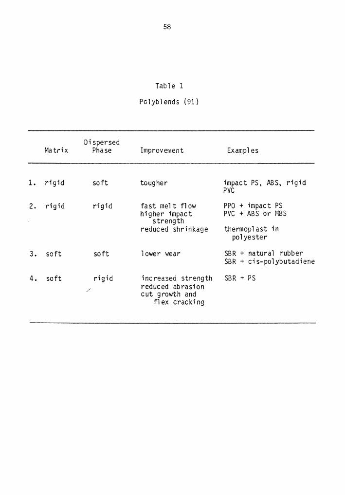
Ma tr ix
1. rigid
2. rigid
3. soft
4. soft
Dispersed Phase
soft
rigid
soft
rigid /
58
Table 1
Polyblends (91)
Improvement Examples
tougher impact PS, ABS, rigid PVC
fast rnel t fl ow PPO + impact PS higher impact
strength PVC + ABS or MBS
reduced shrinkage thermopl ast in polyester
lower wear SBR + natural rubber SBR + cis-polybutadiene
increased strength SBR + PS reduced abrasion cut growth and
flex cracking

Matrix
1. thermoplastics
2. thermo sets
3. vulcanized rubber
4. polyether. polyepoxides, structural resins
59
Table 2
Composites (91)
Dispersed Phase Filler or Reinforcing Material
short glass fibers, beads. hollow spheres, minerals
wood flour. paper. asbestos. clay
carbon black, calcium silicate
long glass fibers. mat or cloth; graphite fibers. boron whiskers

60
stable homogeneous combination which exhibits macroscopic properties
expected of a single-phase material. Homogeneity is defined in terms of
a domain whose dimension is similar to that responsible for macrosopic
properties such as the glass transition and light transparency (95).
Thermodynamics of and methods for determining polymer-polymer
miscibility will be reviewed in terms of polyblends. However, most of
these with a few modifications are applicable to block copolymers, which
generally differ from polyblends by only a few chemical bonds.
1. General Thermodynamics of Polymer-Solvent and Polymer-Polymer Systems
Based on solution thermodynamics of small molecules, using the
lattice concept (93), and taking into account that a polymer segment
must have at least two adjacent sites occupied by polymer segments, one
may arrive at the Flory-Huggins expression for the entropy of mixing of
polymer with solvent (with subscript 1 representing solvent and
subscript 2 representing polymer}.
(95)
where N; and $i are the number of molecules and the volume fraction of
component i, respectively.
With the same assumptions, the enthalpy of mixing can be expressed
as:
~HM = (96)
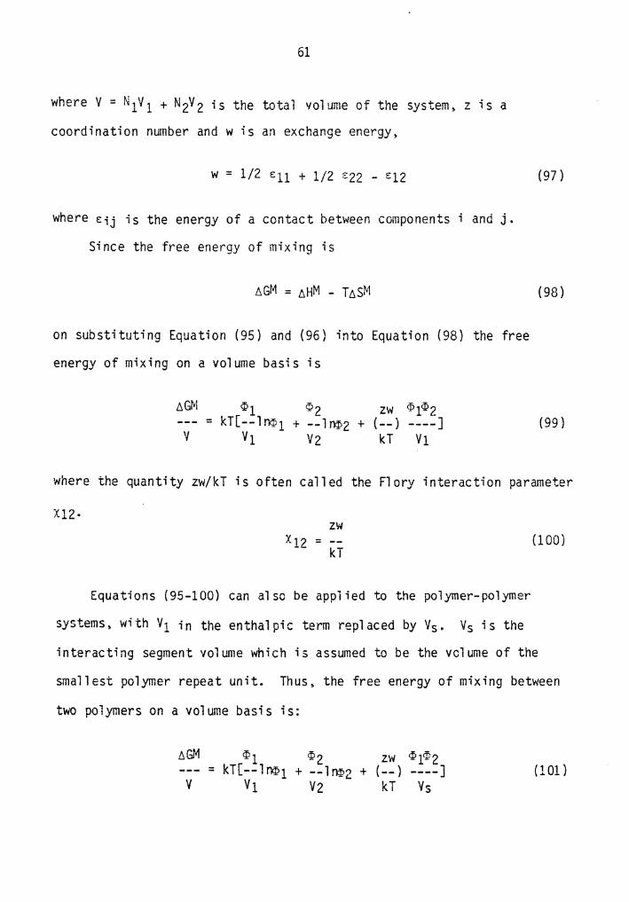
61
where V = NlVl + N2V2 is the total volume of the system, z is a
coordination number and w is an exchange energy,
W = 1/2 Ell + 1/2 S22 - E12 (97)
where Eij is the energy of a contact between components and j.
Since the free energy of mixing is
(98)
on substituting Equation (95) and (96} into Equation (98) the free
energy of mixing on a volume basis is
t.GM 91 92 zw @1~2 = kT[--lr,q;,1 + --11')1)2 + (--) ----] (99)
v Vi v2 kT v1
where the quantity zw/kT is often called the Flory interaction parameter
Xl2· zw (100)
Equations (95-100) can also be applied to the polymer-polymer
systems, with V1 in the enthalpic term replaced by Vs. Vs is the
interacting segment volume which is assumed to be the volume of the
smallest polymer repeat unit. Thus. the free energy of mixing between
two polymers on a volume basis is:
t.GM ~1 ~2 zw <f11~2 = kT[--11')1)1 + --11')1)2 + (--) ----] ( 101)
v V1 v2 kT Vs

62
Because of the large polymer volume. in polymer-polymer systems the
entropic contribution to the free energy of mixing is seen to be
negligible.
2. Stability and Phase Separation Phenomena
Unlike most of solutions of small molecules. in
polymer-polymer systems. a negative free energy of mixing is a necessary
but not a sufficient condition for miscibility. For a homogeneous
single-phase polymer blend, ~GM is negative. However. depending on the
shape and location of the co-existence curve. the same blend could
actually achieve an even lower free energy state by separating into two
phases. Figure 4 (95) gives the free energy of mixing as a function of
concentration in a binary liquid system. The concentration
corresponding to the crest ( <P2 11 <<!>2<<P2') of the free energy curve at T2 fits the situation under consideration. The crest may reflect the
heat of mixing but could equally well spring from a deviation of the
entropy of mixing from mere combinatorial terms (95).
From the Gibbs-Duhem theory of thermodynamic stability (97), a
stable or metastable state can be achieved if and only if
~G < o. and (o2~G/oQ>2) > o T.P (102)
From these criteria, the crest of the free energy curve for T2 can be
divided into two regions. In the region of compositions ranging from
<l>2;sp to <!>2~sp. ( 02~GM/o<!>2)<0, any small perturbation of composition
results in a lower free energy state of the system, thus a spontaneous

Figure 4.
63
T
! I corSGIUt'2 (c:-1:1c:;'; Slc:2.
I 2 1cer.t.c.::1 ,:ircs<Zs
I i !~2
~;J~>J:~~D c.p~'~; ... ~< 2 so1v2n~ -- r; so:,.,,:.:.::
Gibbs Free Energy of Mixing as a Function of Concentration in a Binary Liquid System Showing Partial Miscibility. (95)

64
phase separation may occur, and this region is called the unstable
state. In the region of compositions ranging from <1>2 1 to <1>2;sp and from <j> 11 II { ( )) 2,sp to <1>2 , the stability criteria, Equation 102 are satisfied.
Any small perturbation of composition results in a higher free energy
state of the system. But the state becomes unstable to some finite
perturbation; e.g •• if a nucleus of composition <1>2 11 is fanned, the
composition in its immediate neighborhood will become <1>2 1 • Therefo.re,
this region is called the metastable state.
In the free energy curves of Figure 4, the loci where the stable .
and metastable regions are divided are known as binodals (<1>2 1 ,<1>2 11 ) and
are defined by the equation:
(o~GM/o~)r p = o • or ( l 03)
( 104)
whereµ; andµ;• are the chemical potentials of polymer i in the two
equilibrium phases. The locations where the metastable and the unstable
regions are divided are known as the spinodals, (<1>2:sp.<P2:spl. and
are defined by the equation:
(105)
The critical point or consol ute state is reached when
(106)
A spontaneous phase separation process in the unstable region is

65
referred to as spinodal decomposition. For polymer-polymer systems.
this process usually results in co-continuous phases. Phase separation
in the metastable region is usually via a nucleation and growth
mechanism. For polymer-polymer systems. this process usually results in
a finely dispersed two-phase structure whose final droplet size
as well as inter-particle size depends on the time seal e of tile
experiment and on the rate of diffusion.
3. Solubility Parameter Approach (98,99)
Early attempts at predicting the miscibility of polymer blend
concentrated on the use of Hildebrand's (98) solubility parameter as
popularized by Bohn (99) for polymer-polymer systems.
The solubility parameter is defined as the square root of cohesive
energy density. i.e •• the energy of vaporization per unit volume of
material. and is given the symbol o (98).
o = L~Ev /V ) 1 /2 (107)
Thus. o is proportional to the cohesion of the material or the strength
of attraction between the molecules making up the material.
The solubility parameter approach. which has the utility of
characterizing a system using only component properties without any
system parameters. enables a practitioner to pick compatible components
without having to do any experiments.. With a geometric mean assumption
of the contact en~rgies (98):
{108)

66
which relates them to the cohesive energy density by
.. , t:.E; Ze:ii
6. 2 = = 1 (109) v 2V s
The free energy of mixing of a binary polybiend can be predicted from
the solubility parameters and voluine fractions of the two constituent
polymers by the equation:
t:.GM ( 110)
v
In spite of the tremendous amount of work using this approach,
there have been a great number of dismal failures in predicting
miscibility of polymer blends. Further refinements have been attempted
by a multidimensional approach, breaking the cohesive energy density
into several terms corresponding to the various molecular forces {5).
4. Statistical Mechanical Approaches
A number of equilibrium statistical mechanical approach'=s have
been developed for predicting the complex and peculiar phase behaviors
of polymer-solvent and polymer-polymer systems. In principle, there are
two distinct methods of formulating these theories. The first is the
method of radial distribution functions (100). It generally attempts to
specify the probability of finding polymer segments in particular
conformations. The second method proceeds from an assumed structure
which usually resembles the regulaY- lattice structure of crystalline
solids. The lattice method is considered from two points of view. The
67
first is the purely statistical approach generally referred to as the
approach generally referred to as the Flory-Huggins lattice model, or
the lattice model for short (101-104). The other is developed from the
statistical mechanical partition function and. according to current
literature convention, is referred to as the equation-of-state
approach (105-106).
Thermodynamics of Block Copolymer Systems
Fundamental differences exist between the phase separations
which occurs in a simple mixture of two polymers and that which occurs
in block copolymers. In the fonner case. phase separation is
macroscopic in nature. However, in the case of block copolymers, phase
separation is microscopic; the separate phases, or domains, have
well-defined sizes and shapes. Furthermore, the presence of covalent
bonds in copolymers places some constraints on the number of possible
arrangements, resulting in an appreciable loss in configurational
entropy of mixing. Because of the er.tropy loss, the critical molecular
weight required for !1microphase separation 11 in copolymers is predicted
to be considerably higher than in the analogous homopolymer mixtures.
In an analysis developed by Meier (107) for establishing the
criteria for phase separation in AB diblock copolymers, a surface free
energy contribution representing the interaction of A and B segments at
the domain interface, as well as three contributions responsible for the
entropy decrease of the block copolymer relative to that of a simple
mixture of the components, were taken into account. The three entropic
contributions were referred to as:
68
(1) placement entropy: due to the restriction of the AB covalent
bonds between the domains.
(2) restricted volume entropy: due to the requirement that A
segments remain in domain space A and that B segments remain in the B
domain.
(3) elastic entropy: arising from the perturbation of chain
dimensions in either domain system from their random flight values (93)
which are assumed to hold when the chain is in a homogeneous system.
Using appropriate estimations. the analysis determined that the
critical molecular weight for phase separation would be 2.5-5 times
higher in a block copolymer than in the analogous homopolymer mixture.
The analysis has been extended (108) to estimate the most stable
configuration as a function of block copolymer volume fraction.
Assuming an interfacial tension of 15 dynes/cm, an unperturbed
root-mean-square end-to-end chain dimension (93) to molecular weight
ratio of 7.5xl0-9 (c.g.s unit} and a temperature of 300°K, spherical
domains are preferred below volume fractions of 0.20; cylindrical
domains are preferred between 0.20 and 0.30 with lamellar structure
existing above 0.30. The theoretical predictions are in qualitative
accord with the experimental results on a styrene-butadiene system.
In Meier's extended analysis. the influence of casting solvent on
domain morphology was also considered. Qualitatively. the effect of a
preferential solvent is similar to an increase in the volume fraction of
that component which interacts preferentially with the solvent.
Another treatment was developed by Krause (109.110). It is not

69
limited to a particular type of block copclymer; it is applicable to
mul tibl ock systems. as wel 1 as to m'ixtures of one or more of the
copolymers with the constituent hom·Jpo1ymers. Phase separation
resulting from a crysta11izab1e constituent is also covered in this
model. However. the model is concerned only with thermodynamic phase
separation and not with the morphology of the domain structure.
The prior treatments due to Meier and Krause have all assumed a
discrete interface with no intersegmental mixing. Another approach
considering incorporation of a mixed region at the interface (which is
assumed to exhibit single-phase behavior) has been developed by Leary
and Williams (111-113) for ABA triblock copolymers and by Meier (114)
for AB diblcok copolymers. The results are presumed to be applicable~~
ASA copolymers that could be represented by (A-8/2) diblock structures.
Although the extent of phase mixing at domain boundaries is still
controversial. both approaches, nonetheless, actually predict the
specific microstructure which is thermodynamically favored.
6. Methods for Determining Polymer-Polymer Miscibility (5)
As stated before, the homogeneity of a multicomponent polymer
system is a relative term which can be defined by the technique used to
measure the system. In fact, a compatibility nlllTlber has been defined by
Kaplan (115) as
exp. prcbe size N = (111)
domain size
The experimental probe size in a mechanical test, for example, would be

70
the segmental length associated with the glass transistion phenomenon.
The domain size is the average length in which only one component
exists. For a specific technique, obviously, the larger the
compatibility number. the better the homogeneity of a multi component
po 1 ymer sys tern •
A number of methods having been employed to determine
polymer-polymer miscibility are reviewed in the following. Among them,
only the melting point depression method and NMR method, both of which
were used in this study, are discussed in greater detail.
Glass Transition Temperature
The most commonly used method for determining polymer-polymer
miscibility is through the measurement of the glass transition{ s) in
the blend versus those of the constituent components. A miscible
polymer blend will exhibit a single glass transition between the Tg 1 s of
the components with a sharpness of the transition similar to that of
the components. In the cases of limited miscibility, broadening of the
transition or two separate transitions between those of the constituents
may occur.
A variety of mechanical, dielectric, dilatometric, calorimetric and
thermo-optical methods have been used to determine the glass
transition( s). Despite a 11 un iversal 11 experimental probe size of 150A as
suggested by Kaplan (115), the ievel of molecular mixing associated with
the glass transition method is still uncertain.

71
Microscopy
Direct visual studies by microscopy can determine not only the
presence but also the connectivity or morphology of the phases.
Electron microscopy, with 50A resolution. has shown that heterogeneity
exists even in polyblends having a single glass transition (116,117).
Melting Point Depression
Like the melting point depression phenomena of crystalline or
semicrystall ine polymers in the presence of low molecular weight soluble
compounds, in miscible polyblends. in which one component is
crystallizable. melting point depressions are also observed (118.119).
The general equation for melting point depression of a binary polyblend
is
1 111<1'2 1 [---- + (--
1 --)(l-~2) + x12(l-~2)2J ( 112)
where subscript 1 represents the amorphous polymer and subscript 2
represents the crystall i.zabl e polymer. x12 is the Flory interaction
parameter, Tm is the experimental melting point. Tm 0 is the equilibrium
melting point of pure polymer 2, ~H2 the heat of fusion of 100%
crystalline polymer per mole of repeat unit. Vi and V2 the molar volumes
of repeat units. ~2 the volume fraction, m1 and 1112 the degree of
pol ,ymeri za ti on.
For high molecular weight polyblends. m1 and 1112 are very large.
thus

1 1
Tm 0
72
x12(l-<P2)2 tiH2V 1
( 113)
The equation indicates that a negative x12 will yield a melting point
depression, while a positive interaction parameter will result in a
melting point elevation.
Sol id State NMR
In NMR experiments. the magnitudes of T1. T2. Tlp and other
relaxation parameters are influenced by molecular motfons. Therefore.
comparison of the relaxation times of a polymer mixture or copolymer
with its constituent components usually can reveal the degree of
interaction between the components. Furthermore. in proton NMR. free
induction decays (T2 relaxations) as well as the Ti and T1p relaxations
can be analyzed in terms of the total proton content of each phase. The
experimental probe size of solid state proton NMR is determined by
the maximum spin diffusive path length. which may be given by the
approximate formula ( 120):
L = (60/k)l/2 (114)
where D is the diffusion coefficient and k is the relaxation rate of a
particular relaxation mechanism.
Besides being used for studying the degree of microphase
inhomogeneity and phase separation behavior of compatible polymer blends
(120-125). broadl ine sol id state proton NMR has been employed to
investigate the dynamic and kinetic behaviors of domain structures of

73
block copolymers. including block copolymers of styrene and butadiene
( 126-128), as well as multi block segmented polyurethane systems
(128-132).
The recent advent of the CPMAS high resolution solid state
carbon-13 NMR, in which relaxation parameters (Tl, T2, Tlp• TCH. ri)
usually can be resolved for each individual nuclei, has lead to several
new qualitative conclusions regarding the microstructure and dynamics of
compatible polymer bl ends (133-135) and microphase-separated copolymers
{70,136). For example, Ti's and T1p 'scan be used to characterize
individual main- and side-chain motions in the MHz-and KHz-frequency
ranges, respectively.
Other Methods (5)
Other methods which are frequently used in determining
polymer-polymer miscibility inc1 ude scattering methods, ternary-solution
methods, studies of rheological properties, volumes of mixing, and
heats of mixing as well as infrared, ultraviolet and excimer
fluorescence spectroscopic methods.

Chapter :r CHARACTERIZATION OF STYRENE-ISOPRENE-STYRENE TRIBLOCK
COPOLYMERS AND POLYURETHANES
I. INTRODUCTION
Thermoplastic elastomers (138,139) form an example illustrating the
fact that multicomponent polymer systems can achieve novel properties
unattainable in homopolymers. They are a unique ne\'I class of polymers,
in which the end use properties of vulcanized elastomers are combined
with the processing advantages of thermoplastics.
In general, thermoplastic elastomers are ordered, tri-or
multi-block copolymers of structure A-B-A or (A-B)n, where A represents
a polymer segment which is glassy or crystal 1 ine at service temperatures
but fluid at higher temperatures, and B represents a polymer segment
which is elastomeric at service temperature. Choice of segment type and
length and the weight fractions of A and B are crucial in achieving
elastomeric performance.
The unique properties of the thermoplastic el astomers resui t from
microphase separation or domain formation. It is \'/ell known tl1at the
physical properties and mechanical behaviors of those copolymers are
strongly dependent on the nature and degree of microphase separation
(3,4,137).
Many methods have been used to investigate thermoplastic elastomer
microphase separation. Since the distinction between domains is based
on segmental mobility and this mobility plays a very important role in
determining properties of a material. So nuclear magnetic resonance,

75
having well-established relationships between molecular motions and a
variety of relaxation parameters, is particularly suited to study
domain structure and dynamics of these copolymers.
Pulsed proton NMR has been extensively employed to investigate the
structure and dynamics of solid block and segmented copolymers
{126-132). The main limitations of solid-state proton NMR are poor
resolution and also a very effective spin diffusion among the protons.
On the other hand. solid state C-13 NMR can overcome those problems.
With high pm'ler heteronuclear dipclar decoupling and magic angle
spinning. chemically distinct carbons. in general. have separate C-13
NMR resonances. Furthermore. dipolar decoupling. magic angle spinning,
and cross polarization ~an be used in various combinations to obtain
more detailed information on these copolymers. In this regard. a series
of styrene-isoprene-styrene triblock linear copolymers (SIS) with
different composition and/or molecular weights and a poly(ester)urethane
(PU) based on polybutylene adipate and 4,4i-diphenylmethane diisocyanate
{MDI) were studied by sol id state C-13 NMR and this work is presented in
this chapter.
For the long block styrene-diene-styrene copolymers, it is believed
that domain existence is independent of temperature over a wide range
and the morphology of the domain structure depends primarily on the
composition (128). However, there are disagreements in explaining
certain thermal transitions and viscoelastic behaviors of the
copolymers. Some phenomena can be interpreted by either a diffusive
mixing interface model or a dynamic interaction model which neglects the

76
geometry of the interface between the two phas2s (107-114,127 ,140-145).
In this study, the details of the domain boundaries as well as the
molecular motions (in terms of frequency and orientation) as functions
of composition, molecular weight, and selective casting solvents of the
SIS samples were investigated through measurements and analysis of l3c 1 s
Ti's, bandwidths of resonance peaks (both with and without magic angle
spinning) of the isoprene segments and 13c's T1p's of the styrene
segments.
For the segmented polyurethane, the domain structure and morphology
are more complicated and believed to be time and temperature dependent
(128-130,146-147). In this study, the phase separation, domain
boundaries, and molecular motions of a thermally stable polyurethane
were investigated through the measurements and analysis of 13c•s Ti's,
protons' Tip's (C-13 spectra resolved). The resonance intensities of
spectra obtained at various experimental conditions were also compared.
II. EXPERIMENTAL
A. Samples
SIS Copolymers. Styrene-isoprene-styrene (SIS) linear
triblock copolymers in styrene content ranging from 20 to 60 percent by
weight were obta'ined from the Phillips Petroleum Company. Table 3
summarizes the sample series by styrene content and block number average
molecular weight. The dispersity ratios were provided by Phillips as
determined by gel permeation chromatography. No evidence of

77
Table 3
Composition of SIS Copolymers
Weight Percent M\~/MN S/I /S MN Sample No. Styrene ( 1 o-3) (1 o-3)
10-80-10 20 264/239 24/191/24
20-60-20-H 40 261/238 48/142/48
20-60-20-L 40 114/109 22/65/22
30-40-30 60 81/77 23/31/23
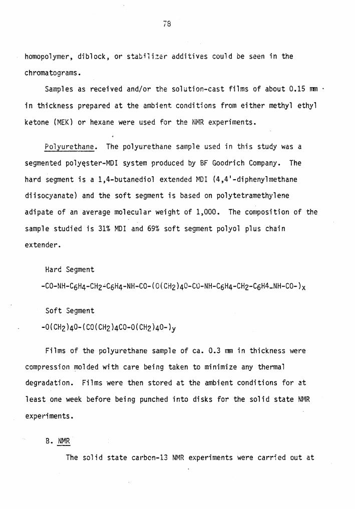
78
homopolymer, diblock, or stabilizer additives could be seen in the
chromatograms.
Samples as received and/or the solution-cast films of about 0.15 nm ·
in thickness prepared at the ambient conditions from either methyl ethyl
ketone (MEK) or hexane were used for the NMR experiments.
Polyurethane. The polyurethane sample used in this study was a
segmented poly~ster-MDI system produced by BF Goodrich Company. The
hard segment is a 1,4-butanediol extended MDI (4,4 1 -diphenylmethane
diisocyanate) and the soft segment is based on polytetramethylene
adipate of an average molecular weight of 1,000. The composition of the
sample studied is 31% MDI and 69% soft segment polyol plus chain
extender.
Hard Segment
-CO-NH-C6H4-CH2~C6H4-NH-CO-(O(CH2)40-CO-NH-C6H4-CH2-C6H4-NH-CO-)x
Soft Segment
-O(CH2)40-(CO(CH2)4CO-O(CH2)40-)y
Films of the polyurethane sample of ca. 0.3 nm in thickness were
compression molded with care being taken to minimize any thermal
degradation. Films were then stored at the ambient conditions for at
least one week before being punched into disks for the solid state NMR
experiments.
B. NMR
The solid state carbcn-13 NMR experiments were carried out at

79
15.0 HMz on a JEOL-60Q spectrometer at room temperature. Various
experimental conditions were employed to obtain the spectra of the
copolymers. These are outlined in the following.
SP-DD-MAS. Single pulse, dipolar decoupled, magic angle spinning
NMR spectra were obtained using a (90°-t) pulse sequence. The 90° pulse
was 7.6 µsin duration.
SP-DD-Static. Single pulse, dipolar decoupled, static NMR spectra
were also obtained using the (90°-t) pulse sequence with the duration of
the 90° pulse adjusted to 7.6 µs.
00-MAS-CP. Dipolar decoupled, magic angle spinning, cress
polarization NMR spectra were obtained at a matched spin-lock cross
polarization transfers employing 1 H1 1 s of 33 KHz with selected contact
and pulse delay times.
The strength of the high power proton dipolar decoupling field was
ca. 33 KHz (7.75 G}. The magic angle spinning experiments were carried
out using a Kel-F 'bullet' type rotor and ca. 2.0 KHz spinning r~tes.
Polymer samples in the form of either rolled thin films or punched disks
were packed into the Kel-F rotor. Each sample represents about 0.5 g of
polymers.
The Hartmann-Hahn condition and the magic angle were adjusted using
the aromatic signal from hexamethylbenzene; the rates of magic angle
spinning were also calibrated using the sidebands of that signal. A11
the spectra were externally referenced to liquid tetramethyl silane
(TMS), based on substitut·ion of hexamethylbenzene (HMB) as the secondary

80
reference and assigning 132.3 and 16.9 ppm to the shifts of the aromatic
and aliphatic carbons, respectively, of HMB relative to liquid TMS.
All the spectra were obtained from 1 K FT with zero filling to a
total of 4 K points. A spectral width of 8000 Hz and an acquisition
time of 64 ms were selected for all the spectra.
l.1 Measurements. T1 values of the carbon-13 nuclei in the isoprene
segments of the SIS copolymers and in the polyurethane were measured ·
using a (180°-~-90°-t) inversion recovery pulse sequence as described in
Chapter I. All the spectra for the T1 measurements were obtained with
dipolar decoupling and magic angle spinning. The time between pulse
sequence, t, was chosen to be ca. five times the longest T1 of the
nuclei of interest. Measurements were made for 6-10 values of ~ which
ranged from 0.001 s to t. Peak heights were used for the analysis of
each T1 data set and T1 values were calculated with a built-in program
in the spectrometer.
llr (13c) Measurements. T1 values of the carbon-13 nuclei in the
styrene segments of the SIS copolymers were measured using a cross
polarization procedure as described in Chapter I. All the spectra for
the 13c T1p measurements in this study were obtained with dipolar
decoupling and magic angle spinning. Six spectra were used for the
calculation which was performed by a program in the spectrometer's
computer.

81
II I. RE SUL TS
A. SIS Copolymer~
1. General Description of Scectra
The isoprene segments of the SIS copolymers are mobile enough
to result in short Ti's for the C-13 nuclei in the order of one tenth of
a second to one second. In contrast the C-13 nuclei in the styrene
segments have long Ti's typical of rigid solids. Figure S(b) shows a
single pulse _{90°-t)-DD-MAS spectrum of the SIS 20-60-20H sample. With
a pulse delay time of three seconds, the resonance signals predominantly
came from tfia isoprene components; nevertheless, weak resonance signals
from the styrene components were detectable. On the other hand, since
higher molecular mobility reduces or even eliminates the effect of
nuclear dipole-dipole interactions, use of a 13c-1H cross polarization
pulse sequence (DO-MAS-CP) for the SIS copolymers resulted in C-13
resonance signals almost exclusively from the styrene segments as shown
in Figure S(a).
Single pulse spectra obtained without spinning (SP-DD-Static} were
still resolvable in terms of the resonance signals of the saturated and
unsaturated carbons of the isoprene segments for all the SIS samples;
some of these were resolvable between the two unsaturated carbons at
half peak height as shown in Figure 7. The resonance signals of these
static spectra were much sharper than those observed for the powder
spectrum cf polydienes studied at low temperature (39), although the
bandwidths were still ca. five-fold broader than those in the spectra
obtained with magic angle spinning.

SIS (20-60-20H)
J./'-·
(b) SP .,../V-..--.J""V'V'-'"Vlr~ .,..-'I • • r --..,,-. "'\I~ t=D0.C--..f1J'o- 7" n~ I I J\Vv lt.~-f'..0.-.;,"'
Q M I I I f I i
100 o ppm
Figure 5. Proton Dipolar Decoupled. Magic Angle Spinning 15.0 MHz C-13 NMR Spectra of the SIS 20-60--20H Copolymer. Spectrum (a} was obtained from 4500 FIO accumulations of a cross polarization pusle sequence with a contact time of 1.5 ms and a pulse delay time of 3.5 s. Spectrum (b) was obtained from 3,000 FID accumulations of a single pulse sequence with a 90° pulse of 7.6 µs and a pusl e delay time of 3 s. Peak assignments are described in the text.
OJ N
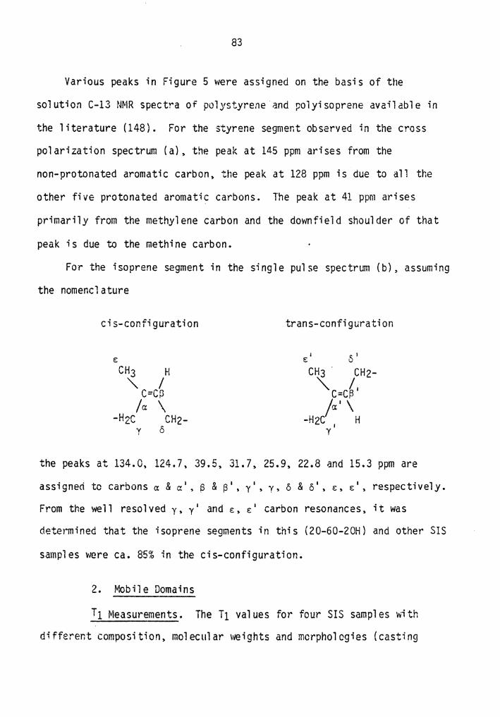
83
Various peaks in Figure 5 were assigned on the basis of the
solution C-13 NMR spec tr-a of polystyrene a.nd polyi soprene available in
the 1 iterature (148). For the styrene segment observed in the cross
polarization spectrum (a). the peak at 145 ppm arises from the
non-protonated aromatic carbon. the peak at 128 ppm is due to all the
other five protonated aromatic carbons. The peak at 41 ppm arises
primarily from the methylene carbon and the downfield shoulder of that
peak is due to the methine carbon.
For the isoprene segment in the single pulse spectrLw (b). assuming
the nomenclature
cis-configuration trans-configuration
the peaks at 134.0, 124.7, 39.5, 31.7, 25.9, 22.8 and 15.3 ppm are ' 't b & I & I I & I I ass 1 g n ea c car on s a: a • p p • y • y • o o • e: • e: • respectively.
From the well resolved y. y' and e:, e:' carbon resonances, it was
determined that the isoprene segments in this (20-60-20H) and other SIS
samples were ca. 85% in the cis-configuration.
2. Mobile Domains
Ti Measurements. The T1 values for four SIS samples with
different composition, molecular \'/eights and rncrphol ogies (casting

84
solvents were different) are listed in Tabie 4. The Ti values for the
two samples with higher i soprene content were measured t\~i ce in order to
show the reproducibility of the method. It appears that within the
experimental errors of this study, the spin-lattice relaxation times in
the mobile domains of the SIS copolymers are independent of the
composition and morphology of the polymers.
Data analysis (149) also indicates that there is a one-component
exponential behavior for the spin-lattice relaxations in the mobile
domains of the SIS samples. Table 5 gives the results of this
treatment of the T1 measurements, where Y(X=O) is the calculated
Mo-M(i;) value of ln ------- at ~=O, or the intercept of the linear regressed
2Mo
Mo-M(~) line: 1 n -------
2Mo
Mo-M( ~) = -~/T1 in a ln -------
2Mo vs. ~ graph such as in Figure
6. In the ideal case of one component, first order relaxation with no
experimental errors, Y(X=O)=O. The variance is defined as
VARIANCE = Mo-Mh) Mo-Mh) 2
~[(ln -------)observed - (ln -------)calculated] 2Mo 2Mo
where N is the number of the observation points used in the calculation.
Since a threshold parameter of 80% was used for all the T1 calculations
to limit error, (i.e •• only when the observed magnetization M(~) Mo-M(~)
satisfied the condition of------- > 0.20 were the data used). the 2Mo
number N could be different in different sets cf data or between
different carbons in an experiment. Again in the ideal case, VARIANCE = o.
/
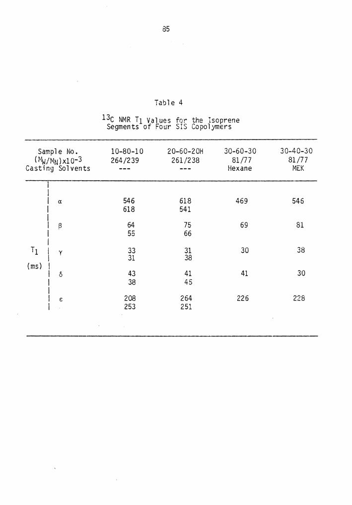
85
Table 4
13c NMR T1 Values for the Isoprene Segments of Four SIS Copolymers
Sample No. 10-80-10 20-60-20H 30-60-30 30-40-30 ( Mw/MtJ) xl o-3 264/239 261/238 81/77 81/77
Casting Sol vents Hexane MEK
I I I a: 546 618 469 546 I 618 541 I I ~ 64 75 69 81 I 55 66 I
T1 I y 33 31 30 38 I 31 38
(ms) I I & 43 41 41 30 I 38 45 I I e: 208 264 226 228 I 253 251

86
Table 5
Data Analysis of the Ti Measurements of the in SIS Copolymers
Isoprene Segments
Sample No. Carbons T1 Y(X=O} Variance N (casting solvents) (ms)
10-80-10 a 546 -0. 0015 o. 0003 9 ~ 64 -0.0531 0. 0001 6 y 33 -0.0414 0.0097 4 6 43 -0.0622 o. 0011 5 e: 208 -0.0070 0. 0015 6
10-80-10 a bi8 -0. OJO/ 0. 0001 I* ~ 55 +0.0083 0.0002 7 y 31 +0.0065 o. 0013 6* 6 38 +0.0273 o. 0017 6 e: 253 -0 .1022 o. 0014 5
20-60-20R a 618 -0. 0344 0.0003 8 ~ 75 -0.0821 0.0003 5 y 31 -0. 0821 0.0014 3 6 41 -0.0727 o. 0019 4 e: 264 -0.0924 0.0003 6
20-60-20H a 541 +0. 02 75 0.0003 I ~ 66 -0.0862 0.0002 8 y 38 -0. 0757 o. 0011 6 6 45 -0. 0432 0.0006 6 e: 251 -0 .1107 0.0045 5
30-40-30 a 469 +O. 0232 o. 0001 !J (Hexane) ~ 69 -0. 0375 0.0036 4
y 30 +0.1381 2 6 41 +0.0166 0.0006 3 e: 226 +O. 0384 0.0002 3
~0-40-30 a 56b -0.0008 0.0000 5 (MEK} ~ 81 -0.1182 0.0026 4
'( 38 -0.0639 0. 0262 3 6 30 +0.1361 2 e: 228 -0.0399 0.0002 4
* Data plotted in Figure 6.

87
0 100 ms 500 ms
-0.5
-1. 0
• 10 ms 50 ms
SIS (10-80-10)
Figure 6.. One Component. First Order Spin·-Lattice Relaxation Behavior of the Isoprene Segments of the SIS 10-80-10 Copolymer.

88
Figure 6 contains a plot of the one-component, first order
spin-lattice relaxations of the isoprene segments for two of the carbons
of the SIS 10-80-10 sample.
Bandwidths With and Without Magic Angle Spinning. Table
6 lists the bandwidths of the single pulse, proton dipolar decoupled
C-13 resonances obtained with magic angle spinning for five SIS samples.
The results show that with magic angle spinning, the bandwidths of the
isoprene carbons in the SIS copolymers are essentially independent of
the composition, molecular weight and morphology {casting solvents)
of the po lyrners.
Table 7 lists the bandwidths of the single pulse, proton dip0lar
decoupled C-13 resonance obtained without spinning the sample for the
two unsaturated isoprene carbons (a: and~) in seven SIS samples. The
results show that higher styrene content and lower molecular weights
tend to result in broader bandwidths for these two carbons, al though the
differences are probably not significant considering the experimental
precision. (Two SIS 10-80-10 samples obtained from the same batch were
studied independently and were found to have a 15% difference in
bandwidt!'ls.) The significant difference in the bandwidths was observed
in the case of the tv10 samp 1 es cast from MEK. The resonance 1 i nes of
the two unsaturated isoprene carbons in these two samples were much
broader than the resonance lines of the other samples studied. They
were overlapped to a large extent, and unlike those peaks in the other
sam~les, spectra were unresolvable at half peak heights. Figure 7
shows static spectra of two SIS 20-60-20H samples: spectrum (a) was

89
Table 6
Bandwidths of the Isoprene Segments in SIS Copolymers (with MAS)
Sample No. 10-80-10 20-60-20H 20-60-20L 30-40-30 30-40-30
(Mw/Mn)xl0-3 264/239 261/238 114/109 81/77 81/77
Casting Solvents Hexane MEK
Carbon*
ex 15 16 14 15 14
* ~ 23 26 26 27 26 vl/2
25 26 27 28 25 y (Hz)
6 21 24 23 29 22
E 15 16 15 14 13
*
Digital resolution= 3.9 Hz
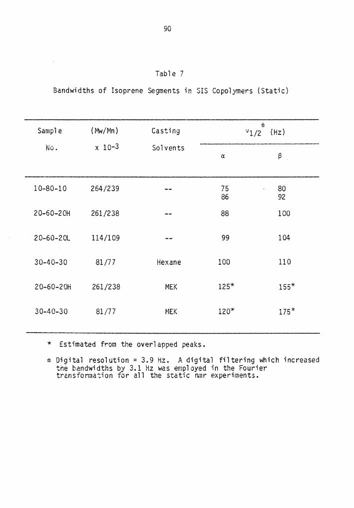
90
Table 7
Bandwidths of Isoprene Segments in SIS Copolymers (Static)
Sample
No.
10-80-10
20-60-20H
20-60-20L
30-40-30
20-60-20H
30-40-30
( Mw/Mn)
x 10-3
264/239
261/238
114/109
81/77
261/238
81/77
Casting
Solvents
Hexane
MEK
MEK
* Estimated from the overlapped peaks.
:f: vl/2 (Hz)
a:
75 80 86 92
88 100
99 104
100 110
125* 155*
120* 175*
:f: Digital resolution = 3.9 Hz. A digital filtering which increased the bandwidths by 3.1 Hz was emp1 oyed in the Fourier transformation for all the static nmr experiments.

SIS (20-60-20H)
(a)
Figure 7. Static Spectra of the SIS 20-60-20H Copolymers. Single pulse proton dipolar decoupled, static C-13 NMR spectra of two SIS 20-60-20H samples. (a) is the spectrum of the sample as recieved, and (b) is the spectrum of the sample cast from MEK. A 90° pulse of 7.6 µsand a pulse delay time of 3 s were used for both spectra.
92
obtained from the sample as received, and spectrum (b) obtained from the
MEK cast sample. Similar differences \'iere al so observed for the SIS
30-40-30 samples cast from hexane and MEK.
3. Rigid Domains
.D.p (13C) Measurements. Table 8 gives the 13c NMR T1p values
for tv-10 SIS 30-40-30 samples cast from two different sol vents (hexane
and MEK). Data analysis results are also listed in the table, where the
definitions of Y(X=O), VARIANCE and N are the same
mobile domains. except
as those described in Mh)
that ln(----) was Mo
the T1 measurements for the Mo-Mh)
used instead of ln(-------) 2Mo
in the analysis. The values of T1p were
calculated from the peak intensities at 145,128 and 41 ppm. which
corresponded to the non-protonated aromatic, protonated aromatic and
predominant methine overlapped with methylene carbons. respectively.
Within the experimental conditions (limited sensitivity. resolution and
data points. as shown in Figure 8). no significant difference between
13c T1p of these two samples could be distinguished.
B. Polyurethane
1. General Description of Spectra
Unlike the SIS copolymers investigations. with the single
(SP-DD-MAS) and with the cross polarization (DD-MAS-CP) pusle sequences.
C-13 NMR resonance signals were obtained from both the hard and the soft
segments of the polyurethane. However, the relative intensities of the
two segments depended on the experimental conditions. Figure 9
illustrates the solid state C-13 NMR spectra of the polyurethane

93
Table 8
13c NMR T1p Values for the Styrene Segments in Two SIS 30--40-30 Samples Cast from Different Solvents
Casting Solvents
Hexane
MEK
Carbons (ppr.:)
C1
(145)
C2-5 (128)
CH
(41)
C1
(145)
C2-5
(128}
CH
(41)
Numbering Scheme:
T1p (ms)
47.2
12 .1
9.3
32.5
14.8
lC .5
Data Analysis
Y(x=O) Variance N
-0.0376 0.0020 3
-0.0528 0.0000 3
-0.2178 0.0068 3
-0 .0775 0.0017 4
-0.0792 0.0007 3
-0.3048 0.0004 3
(CH2-CH) 2""..i_6 101 3 ,.....s 'i+

-,;.
SIS (J0-40-JO) T1p( 13c) Measurement _by CE.._Pul.s._a _ S equ enc e ____ _
!!Oy Hoc 9Qy 90y-· ~
'HI lllH H,y
I-1 --- .----1
I
lms /'~ ! ... ~·
3ms 4~~· holJ. ~"'
lOms
JOms I~~ .J\k¥""'tV~W'i
lOOms ~,.,.... .............. ,,..,""""..., .. -..,..,..
Figure 8. 13c T1p Measurement for the Styrene Segments of the SIS 30-40-30 Samples Cast from Hexane. A contact time of 1. 5 ms a11d a pulse delay time of 3. 5 s were used. 600 scans were accumulated for each spectrum.
c..o +=-

ls 2h 4h
3h
6h
POLY1J RETHANE
as
7h
.------ r~---.-------.---=---..----.---T • • • • 1 • • • . • 1 • • • • 1 , . r- '.
200 100 0 ppm ~ Figure 9. Solution and Sol id State C-13 NMR Spectra of the Polyester-MDI Polyurethane with 31 wt% MDI.
(a) and (b) are solid state spectra obtained with proton dipolar decoupling and magic angle spinning: spectrum (a) employed a cross. polarization pulse sequence with a contact time of 1.0 ms and a pulse delay time of 4 s. spectrum (b) employed a single pulse sequence with a 90° pulse of 7.6 µsand a pulse delay time of 3.5 s. 7000 and 2000 scans were accumulated for spectra (a) and (b). respectively. (c) is a proton noise-decoupled 15.0 MHz C-13 spectrum from a hexadeteriodimethylsulfoxide (DMSO-d6) solution at the ambient condition. Spectrum (c) was carried out in different probe of the same spectrometer from which spectra (a) and (b) were obtained. The internal standard of spectrum (c) is the central peak of DMSO-d6, which occurs at 39. 5 ppm with respect to TMS. Sol vent peaks as well as the peak of MDI methylene carbon which occurs in the midst of them were deleted in the Figure.
l.D
'f'

96
obtained with both pulse sequences. The same figure also gives a proton
noise-decoupled 15.0 MHz solution C-13 NMR spectrum in
hexadeuteriodimethylsulfoxide (DMSO-d6). Peak assignments for the
solution spectrum are listed in Table 9 •
. In Table 9 the following convention of identification was employed.
Hard Segment
MDI
Butanedi ol
Soft Segment
Polyol
-CO-NH-t t
(2) (3)
(6)(5)(9) ~ ~ ~
-NH-CO-
( 11) ~·
-(-OCH2CH2CH2CH20-)-t
(7}
(13) {12) ~ ~
-O(CH2)40-(-CO-CH2CH2CH2CH2-CO-OCH2CH2CH2CH20-)-. t t t y
{1)(10) (8)
2. .Ii Measurements
The single pulse solid state C-13 spectrum with a pulse delay
time of 3.5 s gives resonances from both the hard and soft segments as
shown in Figure 9b. However, a comparison of single pulse sp~ctral
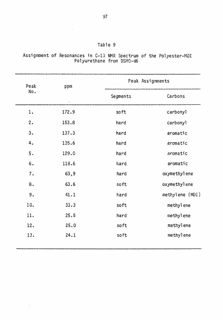
97
Table 9
Assignment of Resonances in C-13 NMR Spectrum of the Polyester-MDI Polyurethane from DSMO-d6
Peak Assignments Peak ppm
No. Segments Carbons
1. 172.9 soft carbonyl
2. 153.8 hard carbonyl
3. 137.3 hard aromatic
4. 135.6 hard aromatic
5. 129.0 hard aromatic
6. 118.6 hard aromatic
7. 63,9 hard oxymethylene
8. 63 .6 soft oxymethylene
9. 41.1 hard methylene (MDI )
10. 33.3 soft methylene
11. 25.5 hard methylene
12. 25.0 soft methylene
13. 24.1 soft methylene

98
intensities with the cross po1arization spectrum. Figure 9a. and the
solution spectrum, Figure 9c. shows that the relative intensities of the
carbons in the hard segments are much weaker in the single pulse
spectrum. This suggests that. in general. the Ti values of the C-13
nuclei in the hard segments should be 1 anger than those in the soft
segments. From a progressive saturation experiment, Ti values for the
carbonyl and the non-protonated aromatic carbons of the hard segment
were estimated to be ca. 5 sec.
T 1 values for the two most intense peaks of the single pulse spectrum were measured with the inversion-recovery method. The peak at
173 ppm came exclusively from the carbonyl carbon of the soft segment.
The unresolved peak at 25 ppm came from the methylene carbons of both
the hard and the soft segments. It should be noted that the
contribution from the hard segment was expected to be small in view of
the intensities of the solution spectrum and as a result of the longer
T1 of the carbons in the hard segment. Since Ti values for the two
peaks differ by more than an order of magnitude, two independent
experiments with different~ values between ·the 180° and the 90° pulses
and pulse delay times were carried out. These results. as well as the
data analysis. are given in Table 10. The data analysis reveals
characteristic one-component~ first order spin-lattice relaxation
behavior. Good correlation is especially noticed for the completely
resolved carbonyl peak. The exponential spin-lattice relaxaion behavior
for both peaks was plotted and is shown in Figure 10.

99
Table 10
13c NMR T 1 Values for the Two Most Intense Peaks of the Polyester-MDI Polyurethane with 31 wt% MDI
Carbons (ppm)
Carbonyl {173)
Methylene (25)
T1
1.128s
66.3 ms
Data Analysis
Y(x=O) Variance N
-0. 0160 0.0006 8
-0. 0635 o. 0013 7

0 100 ms
_,,Q,S
-1.0
10 ms
....... -- ---·
100
500 ms
50 ms
POLYURETHANE
0 II -c-
T
Figure 10. One Component~ First Order Spin-Lattice Relaxation Behavior of the Polyurethane with 31 wt% MDI.
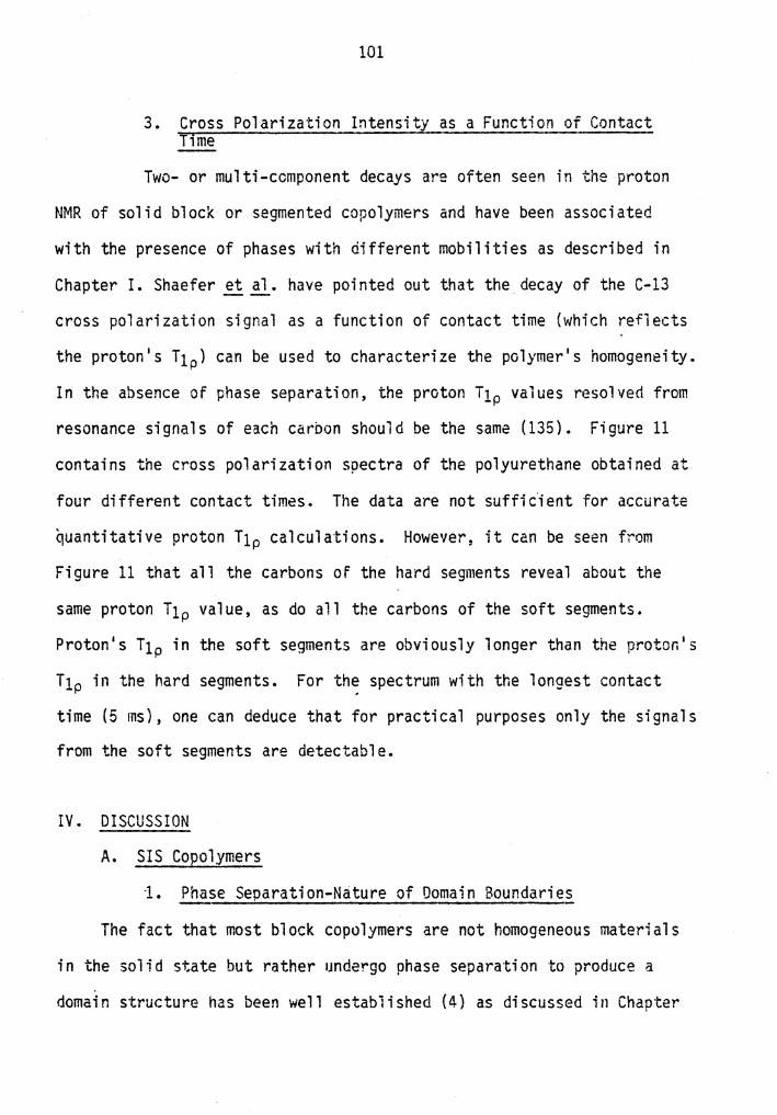
101
3. Cross Polarization Intensity as a Function of Contact ime
Two- or multi-ccmponent decays are often seen in the proton
NMR of solid block or segmented copolymers and have been associated
with the presence of phases with different mobilities as described in
Chapter I. Shaefer et A!_. have pointed out that the_ decay of the C-13
cross polarization signal as a function of contact time (which reflects
the proton 1 s T1p) can be used to characterize the polymer 1 s homogeneity.
In the absence of phase separation, the proton T1p values resolved from
resonance signals of each carbon should be the same (135). Figure 11
contains the cross polarization spectra of the polyurethane obtained at
four different contact times. The data are not suffi dent for accurate
quantitative proton Tlp calculations. However, it can be seen from
Figure 11 that all the carbons of the hard segments reveal about the
same proton T1p value, as do all the carbons of the soft segments.
Proton's T1p in the soft segments are obviously longer than the protor.'s
T1p in the hard segments. For the spectrum with the longest contact . time (5 ms), one can deduce that for practical purposes only the signals
from the soft segments are detectable.
IV. DISCUSSION
A. SIS Copolymers
1. Phase Separation-Nature of Domain Boundaries
The fact that most block copolymers are not homogeneous materials
in the solid state but rather undergo phase separation to produce a
domain structure has been well estabiished (4) as discussed in Chapter

POLYURETHANE Contact Time
~· .. ,.~
l.5ms ·~··~
J.Oms ~,,... ............... ___
5.0ms ~___,.
5 6 128 . BS S
s . 2_ - ~ I I 10 13" ___ ·1__..J_LJLLJ 7l ' ti ___ ~
, '206 . , , , • . , . '1ob , . . . ' , , , , ol ppm , ·...----.
Figure 11. DD-MAS-CP 15.0 MHz C-13 NMR Spectra of the Polyester-MDI Polyurethane Obtained at Various Contact times. All the solid state spectra were obtained from 7,000 FID accumulations and a pulse delay time of 4 s. Solution spectrum of Figure 9(c) is shown on the bottom for peak assignments.
........ 0 N

103
I. However, there has been considerable speculation and disagreement in
the Hterature concerning the details of the domain interface in block
copolymers, especially the AB and ABA block copolymers prepared from
styrene and a diene monomer {isoprene or butadiene), viz, the 11 two-phase 11 vs. "three-phase" system, or a 1ithick 11 vs. 11 thin 11 interface
also as discussed in Chapter I.
In this study, phase separation in the SIS copolymers is evident
from the distinct dynamic properties of the carbons in the styrene
segments and in the isoprene segments. As is shown in Figure 5, both
segments can be observed selectively with different NMR experimental
conditions.
The fact that no resonance signals from the isoprene segments were
detectable in the cross polarization spectrum suggests that even though
substantial mixed phases may exist, the styrene components in the mixed
phases are not able to immobilize the isoprene segments to produce any
substantial residual nuclear dipole-dipole interaction. This behavior
which was observed can not be rationalized on the basis of a mixed phase
system. Furthermore, the basically independent nature of the isoprene
13c T1 values on molecular weight and composition of the blocks together
with the linearity of the exponential decay in the T1 measurements also
suggests that sharp boundaries exist between the styrene and isoprene
domains for the samples we studied.
Theoretically, the isoprene segments in any "mixed phases 11 would be
expected to have longer T1 values than those in the pure isoprene
domains due to the overall reduced mobility in the former case. The
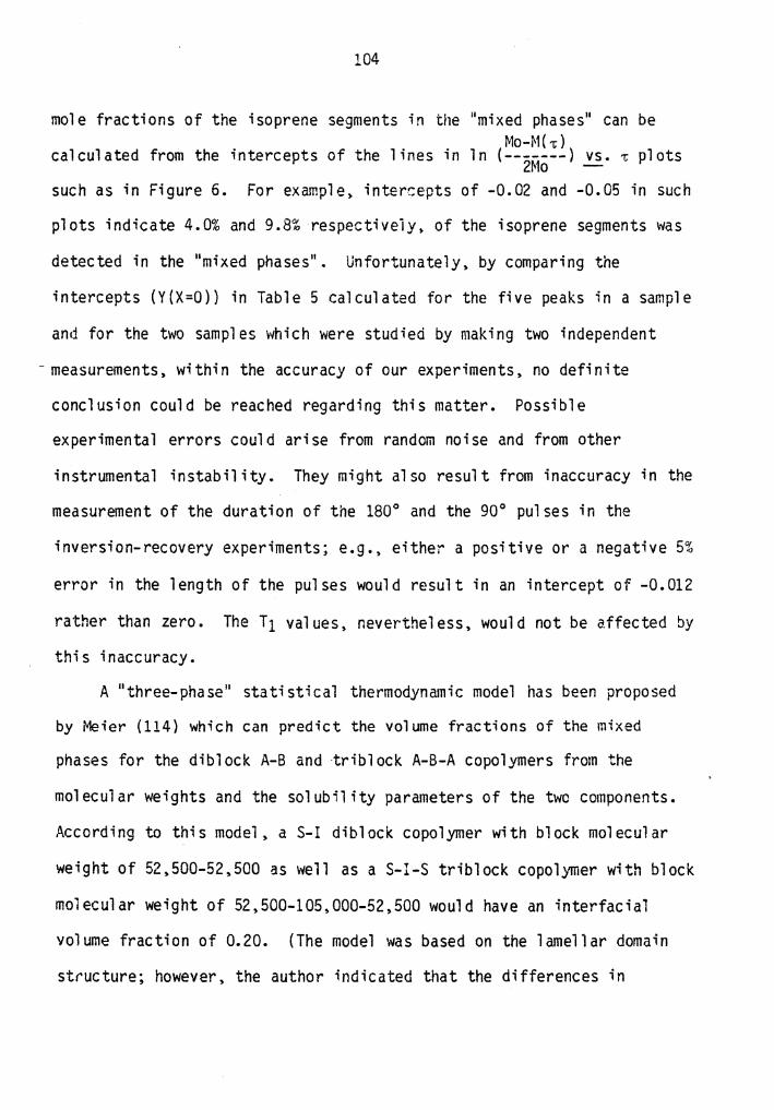
104
mole fractions of the isoprene segments in the "mixed phases" can be Mo-M(-c)
calculated from the intercepts of the lines in ln (--2M0--) ~· T, plots
such as in Figure 6. For example, intercepts of -0.02 and -0.05 in such
plots indicate 4.0% and 9.8% respectiveiy, of the isoprene segments was
detected in the "mixed phases 11 • Unfortunately, by comparing the
intercepts (Y(X=O}} in Table 5 calculated for the five peaks in a sample
and for the two samples which were studied by making two independent
- measurements. within the accuracy of our experiments. no definite
conclusion could be reached regarding this matter. Possible
experimental errors could arise from random noise and from other
instrumental instability. They might also result from inaccuracy in the
measurement of the duration of the 180° and the 90° pulses in the
inversion-recovery experiments; e.g., either a positive or a negative 5%
error in the length of the pulses would result in an intercept of -0.012
rather than zero. The Ti values, nevertheless. would not be affected by
this inaccuracy.
A 11 three-phase 11 statistical thermodynamic model has been proposed
by Meier (114} which can predict the volume fractions of the mixed
phases for the di block A-B and -tribl ock A-B-A copolymers from the
molecular weights and the solubility parameters of the two components.
According to this model. a S-I diblock copolymer with block molecular
weight of 52,500-52,500 as well as a S-I-S triblock copolymer with block
molecular weight of 52,500-105,000-52,500 would have an interfacia1
volume fraction of 0.20. (The model was based on the lamellar domain
structure; however. the author indicated that the differences in

105
interfacial properties between the different possible domain structures
were not large.) AS-I diblock copolymer of the same molecular weight
(52,500-52,500) was investigated by Hasegawa, et~., (150). From
small-angle x-ray scattering data, it was concluded that the interface
constitutes a neg1igible fraction of the polymer, ca. 5-10%.
Our data, although inconclusive, tend to support the thin interface
argument with two lines of evidence. First, from the data treatment of
the peaks of the cis-a carbon {which has the highest intensity among the
peaks and is completely resolved from the other chemically different
carbons as well as from the a-carbon of the trans-isomer), the
intercepts were negligible. They ranged from -0.0344 to +0.0275 for the
six T1 measurements. Very good data correlations were also observed for
the T1 measurements of the cis-a carbon peak, with the largest VARIANCE
obtained to be 0.0003. Second, if a large amount of mixed phases were
indeed present, as it was calculated by the Meier's model to be 20% by
volume for the SIS triblock copolymers of block molecular weights of
52,500-105,000-52,500, then the SIS 20-60-20H sample having the closest
composition and block molecular weights (48,000-142,000-48;000) among
the samples would also be expected to have a substantial amount of mixed
phases. That should have produced some detectable isoprene resonance
signals in the cross polarization spectrum (Figure 5{a)).
2. Molecular Motion in the Mobile Domains
The fact that no isoprene carbons could be observed in the
cross polarization spectra suggests that, in terms of frequencies,
motion of these carbons is essentially "liquid-like" and is fast on the

106
time scale of dipolar interaction (ca. 105 Hz). The bandwidths observed
in the static spectra can be narrowed further by magic angle spinning.
This additionally indicates that the motions are anisotropic. However,
the bandwidths of the sp2 hybridized carbons in the static spectra are
in the order of 100 Hz as compared to the typical values in the rigid
anisotropic lattice which are found to be ca. 2000 Hz in a magnetic
field of 1.4 Tesla (39). This reveals that motions averase the chemical
shift anisotropy to a large extent in the isoprene segments.
Nevertheless. the residual chemical shift anisotropy is the primary
source of line broadening observed in the static spectra.
The T1 values (Table 4) and bandwidths with magic angle spinning
(Table 6) indicate that the rates of these thermal motions is
independent of the composition. molecular weight and morph0logy of the
SIS samples in the ranges studied. This is consistent with the reports
based on calorimetric (145,151). viscoelastic (142). broa~line proton
NMR (127) and esr spin-probe (143) studies which concluded that the
diene's Tg of the SI and SIS (or SB and SBS) copolymers is not a strong
f•Jnction of composition and molecular weight.
Even though the T1 values and the bandwidths obtain~d with magic ,
angle spinning are independent of composition. molecular \'1eight and
morphology of the SIS copolymers studied. it appears that the bandwidths
of the static spectra depends on the morphology of the samples (Table 7
and Figure 7). The morphology of the SIS copolymers actually depends on
a variety of parameters. as discussed in Chapter I. For the long block
samples, in general. the most important variable seems to be the volume
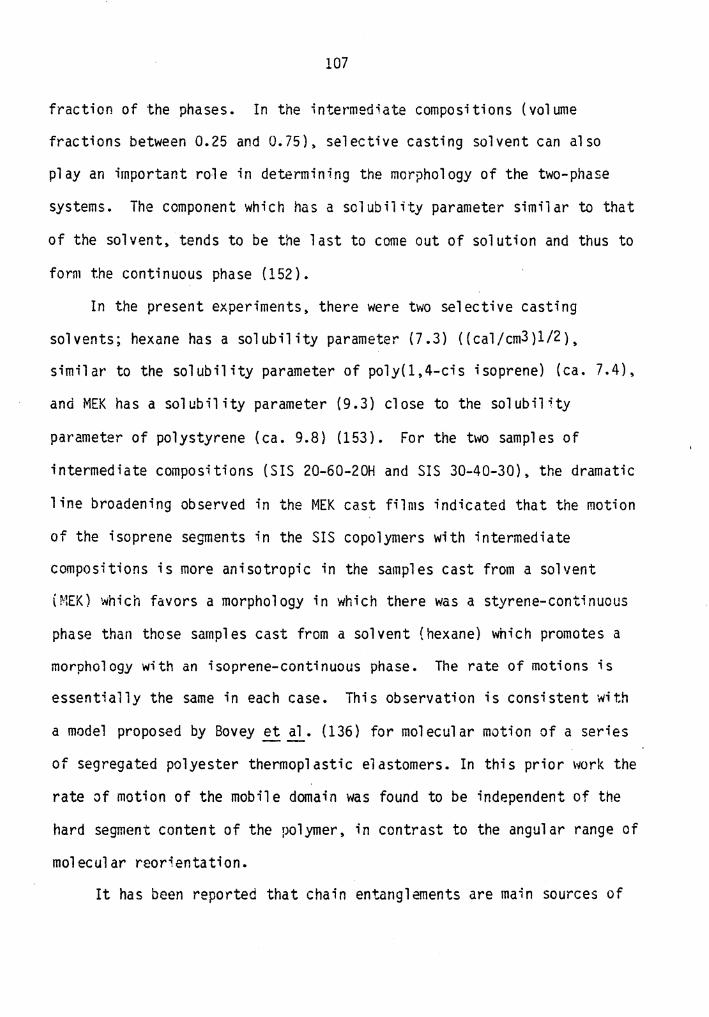
107
fraction of the phases. In the intermediate compositions (volume
fractions between 0.25 and 0.75). selective casting solvent can also
play an important role in determining the morphology of the two-phase
systems. The component which has a solubility parameter similar to that
of the solvent. tends to be the last to come out of solution and thus to
form the continuous phase (152).
In the present experiments. there were two selective casting
solvents; hexane has a solubility parameter (7.3) ((cal/cm3)1/2),
similar to the solubility parameter of poly(l,4-cis isoprene) (ca. 7.4).
and MEK has a solubility parameter (9.3) close to the solubility
parameter of polystyrene (ca. 9.8) (153). For the tv~o samples of
intermediate compositions (SIS 20-60-20H and SIS 30-40-30), the dramatic
line broadening observed in the MEK cast films indicated that the motion
of the isoprene segments in the SIS copolymers with intermediate
compositions is more anisotropic in the samples cast from a solvent
(MEK) which favors a morphology in which there was a styrene-continuous
phase than those samples cast from a solvent (hexane) which promotes a
morphology with an isoprene-continuous phase. The rate of motions is
essentially the same in each case. This observation is consistent with
a model proposed by Bovey et~· {136) for molecular motion of a series
of segregated polyester thermoplastic el astomers. In this prior \vork the
rate of motion of the mobile domain was found to be independent of the
hard segment content of the polymer. in contrast to the angular range of
molecular reorientation.
It has been reported that chain entanglements are main sources of

108
13c NMR line broadening of the isoprene peaks in high molecular weight
SI copolymers {i45). This may also explain the results of the present
bandwidth study of the static spectra. It suggests that the degree of
chain entanglement among the isoprene segments of a SIS sample cast from
a "poor" solvent of polyisoprene might be higher than that of the same
sample cast from a "good" solvent of polyisoprene. This represents an
area for future studies.
3. Molecular Motion in the Rigid Domains
Long Ti's of the styrene carbons in the SIS copolymers as
evident from the disproportionate resonance intensities of the singl~
pulse spectra with a short pulse delay time of 3 sec. {Figure 5)
indicate that there was a low density of motions of the styrene
components in the MHz region. This is consistent with the results for
glassy polymers without methyl or other groups of substantially higher
mobility (38).
The long Ti's of the styrene carbons make it infeasible to
investigate their behavior with conventional inversion-recovery or
progressive saturation methods. The rotating frame relaxation times
{Tip's) which enable one to obtain information on molecular processes in
a much lower frequency range than those encountered in ordinary T1
studies (KHz instead of MHz) are usually much shorter than the Ti's in
the case of rigid solid samples. This, together with the advantages of
the cross polarization process, makes it feasible to do i3c Tip
experiments on the styrene components.

109
The glass transition depression of the styrene components in
styrene-diene copolymers has been compared to that of the pure polymers
of comparable molecular weight (127,142,143,151). In the same studies,
the effect of composition and the molecular \.,.eight of the diene
component on the styrene's T9 was found to be inconsequential. However,
the effect of morphology on the molecules motions was not reported in
these papers. The results of the 13c T1p experiments of this current
study for the two SIS 30-40-30 samples cast from different solvents
indicated that selective casting solvents. or morphology, had no strong
influence on the molecular motions of the rigid domains.
Data analysis of the styrene's 13C T1p measurements revealed poorer
correlations and larger intercepts than those obtained from the
isoprene's 13c Tl measurements. However, besides the poor sensitivity
and resolution of the T lp experiment, the inherent dynamic heterogeni ty
of a polymer glass can result in 13c Tip dispersion even for a
homopolymer {38,154). Thus, it would be more difficult and complicated
to estimate the interfacial regions of the SIS copolymers from the data
analysis of the styrene's 13c T1p measurements.
B. Polyurethane
1. Phase Separation
The morphology of urethane block copolymers is complicated not
only by the two-phase structure as also found in the styrene-diene
systems. but also by the possibilities of ether physical phenomena, such
as crystal 1 ization and hydrogen bonding in beth segments (155). The
time and temperature dependence of the morphology of the segregated

110
polyurethanes has been studied. It is believed that the domain
interfaces of the polymers are diffusive and the degree of domain
structure is a function of temperature and time (128-130,146,147).
In this C-13 NMR study, due to the limitation of sensitivity for
the natural abundance sample, it was not possible to investigate the
morphological kinetic behavior in the time scale of minutes and hours.
However, conclusions regarding phase-separation and the sharpness of the
interfacial boundary can be drawn from the present results for the
polyurethane, given a specific composition and thermal history.
First, the fact that C-13 cross polarization spectra as a function
of contact times revealed two sets of proton's T1p, corresponding to
those of the protons of the hard and soft segments, indicates phase
separation between the hard and soft segments of the polyurethane.
Second, the fact that the C-13 resonance of the soft segments can
be-selectively observed with a iong contact time (Figure 11} as well as
an observed one-component first-order spin-lattice relaxation behavior
of the soft segment carbons (Figure 10 and Table 10) indicated sharp
domain boundaries for this specific polyurethane sample. This was
especially true for the carbonyl carbon which has the highest peak
intensity in the single pulse spectra and is completely resolved form
the resonance of the other carbons.
2. Molecular Motions
The fact that C-13 NMR resonances of both segments of the
polyurethane can be observed from both the single pulse and the cross
polarization spectra (Figure 9} indicated that the molecular mobilities

111
in the soft and in the hard domains were not as dramatically different
as was found in the case of the SIS copolymers. This is not unexpected,
since, the T9 of the soft polytetramethylene adipate segment in the
polyurethane is slightly above room temperature (37°C from a proton NMR
study of a 35% MDI polyurethane sample of the same constituent monomers
and prepared by the same company as the sample of this study (129)),
while Tg of the polyisoprene is well below the room temperature (ca.
-73°C).
Further studies comparing the resonance intensities of the two
spectra of Figure 10 (a CP spectrum with a contact time of 1 ms which
obtained approximately the maximum intensities as a function of contact
time and go 0 SP spectrum with a pulse delay time of 3.5 s) as well as a
go 0 SP spectrum with a pulse delay time of 20 sec. (Table 11) draw two
lines of conclusions:
First, the resonance intensities of the soft segment carbons were
not enhanced by the CP process. This is an indication that nuclear
dipolar interactions in the mobile domains, although observable, are
attenuated by the molecular motions to a 1 arge extent. Much weaker
relative intensities for the carbonyl carbons (of both the soft and hard
segments) in the CP spectrum are expected due to the long cross
rel ax a ti on times of non-protonated carbons.
Second, the resonance intensities of the hard segment carbons
{studied from the aromatic region} show a small enhancement by the CP
process. The enhancement (1.2) is significantly smaller than the
theoretical limit for a rigid lattice (4.0). This together with the

112
Table 11
Relative 13c NMR Peak Intensities of the Polyurethane Obtained at Various Experimental Conditions
Pulse Sequence 90°-sP 90°-SP CP (lms)
Pulse Delay Time 3.5s 20s 4s
Relative 172. 9 ppm ( s) 0. 96 1.- 0.18 Peak I ntensi ti es
153.8 ppm (H) 0.86 1.- 0.82 (per scan per mg)
137.3 ppm (H) 0.85 1.- 1.22
63.6 ppm (S*) 1.10 1.- 0.86
33.3 ppm (S*) 1.11 1.- 0.86
25.0 ppm (S*) 1.01 1.- 0.67
* unresolvable from resonance signals of the hard segment nuclei

113
relative short Tl values of the hard segment carbons of approximately 5
sec. according to the peak intensities at 153.8 and 137.3 ppm, indicates
that for the rigid domains of the polyurethane at room temperature, high
frequency motions (MHz), although more restricted relative to the mobile ~
domains, are less restricted compared to most of the glassy polymers
without fast relaxation sidechains.
Finally, although spin-lattice times of the hard segment carbons
were observed, as expected, to be longer than those of the soft segment
carbons. However, the proton's Tlp was longer in the mobile domain than
in the _rigid domain. This is not what would be expected if the rotating
frame relaxation is dominated by a spin-lattice process, as has been
reported in the literature from the study of some glassy polymers (38,
154). Therefore, for the polyurethane, at least in the hard domain, the
proton's rotating frame relaxation had a substantial contribution from
the spin-spin process.
V. CONCLUSIONS
The principal conclusions of this chapter are summarized as
follows:
SIS Copolymers
1. With dipolar decoupling and magic angle spinning, high
resolution C-13 NMR spectra could be obtained at room temperature for
the high molecular weight isoprene segments of the SIS copolymers.
Using a conventional liquid probe, however, high resolution C-13 NMR
spectra were obtained only for the low molecular weight diene samples or

114
fer high molecular weight diene samples at an elevated temperature.
2. C-13 resonances of both segments of the SIS copolymers could be
selectively observed with different experimental conditions and this is
a strong indication of phase separation. Cross polarization pulse
sequences (DD-MAS-GP} gave resonance signals almost exclusively from the
carbons of the styrene segments. Single pulse sequence (SP-DD-MAS) with
a short pulse delay time (3s) gave resonance signals predominantly due
to the carbons of the isoprene components.
3. Sharp interfacial boundaries in the samples studied are
indicated by two facts: First. the independence of the isoprene 13c i1
values on the molecular weights and compositions of the copolymers.
Second. there was clearly a one component. first order spin-lattice
relaxation behavior of the C-13 nuclei of the isoprene segments. In
principle. the mole fraction of the isoprene segments in the interfacia1
regions can be estimated from the fraction of the isoprene carbons with
longer T1. This method did not give accurate results on the interfaces
for the high molecular weight samples we studied. However. it might be
possible to apply this method to the study of low molecular weight
samples of a similar type which could have higher interfacial mixed
composition fractions.
4. Non-cross-pol ari zabil i ty of the nuclei in the i soprene segments
indicated high moieculdr mobility in the soft domains. The motions are
essentially 11 liquid-like 11 in terms of frequencies.
5. Magic angle spi nnir.g narrowed the bilndwi dths of the i soprene
C-13 resonances by factors of 5 to 10. This indicates that motion of

115
the isoprene segments is anisotropic due to the restictions imposed
either by the rigid styrene domains and/or chain entanglements among the
isoprene segments.
6. The effect of selective casting so"lvents on the bandwidth of
the isoprene resonances in the static spectra indicated that the motion
of the isoprene segments in the SIS copolymers was more anisotropic in
the samples cast from a "poor" solvent of polyisoprene than in those
cast from a "good" solvent. This could result from different morphology
and/or a higher degree of isoprene chain entanglements.
7. Motion in the hard domains was not a strong function of the
selective casting solvents or the morphology.
Polyurethane
1. Phase separation was indicated by two sets of proton's Tip
(corresponding to those of the hard and soft segment protons) measured
from the C-13 resonances as a function of the CP contact time.
2. Sharpness of domain boundaries in the sample studied is
indicated by two facts: (i) resonance signals of the soft segments were
selectively observed using a long CP contact time. (ii) one-component.
first-order. spin-lattice relaxation behavior of the C-13 nuclei of the
soft segments was found.
3. Although the resonances of the soft segments can be obtained
with a cross polarization process. comparison of the resonance
intensities of the CP and the SP spectra. however. indicated that the
nuclear dipolar interactions in the mobile domains were attenuated by
the molecular motions to a large extent.

115
4. Judging from the relatively small signal enhancement by the CP
process as well as short 13C T1' s, high frequency motions in the rigid
domains of the polyurethane. although more resticted than those in the
mobile domains. are less restricted when compared to those in most of
the glassy polymers without fast relaxation sidechains.
5. The fact that proton's T1p in the mobile domains \~re longer
than those in the rigid domains indicated that with the experimental
conditions of a spin-locking field of 7.75 gauss, spin-spin process as
well as spin-lattice process played· an important role in the rotating
frame relaxation of the polyurethane sample studied.

I. INTRODUCTION
Chapter III
COMPATIBILITY STUDIES OF POLYMER BLENDS CONTAINING POLY{VINYLIDENE FLUORIDE)
As a result of interest in polymer-polymer interactions in the
solid state and the continued growth in commercial applications of
polymer blends (1,2,5,6), a variety of experimental techniques have been
employed to investigate polymer-polymer miscibility as was discussed in
Chapter I. However, different methods reveal different facets of the
nature of the mixing process; consequently, no single method has
answered all the interesting questions at the molecular level (156,157).
Hence, it was desirable to try to extend the range of the potential
tools available for analysis in this important area and to compare the
results to those obtained from the previous efforts.
High resolution solid state C-13 NMR has certain advantages over
most of the other techniques due to its capability for probing the
possible interactions at the molecular level. It has been used to study
polymer-polymer miscibility through the measurement of T1, T2, T1p and
other relaxation parameters (133-135). However, the studies reported in
this chapter were undertaken to examine polymer blends of
poly(vinylidene fluoride) from rather a unique point of view (158,159).
For most organic polymers in the solid state, use of MAS in
combination with high power 13c-1H dipolar decoupling and cross
polarization will result in a high resolution carbon-13 NMR spectra.
One observes, though, that even with all three techniques applied,
117

118
complicated spectra result in the case of poiymers which contain other
NMR active nuclei (other than 13c and 'H) having high natural abundance
and strong nuclear magnetic moments. Usually quite broad, or in some
cases, completely featureless spectra are obtained due to dipolar
coupling between the carbon-13 nuclei and the 'other nuclei'.
Poly(vinylidene fluoride), (PVF2), for instance, when analyzed without
simultaneous decoupling of the fluorine-19 and the protons produces a
13c frequency domain spectrum which is completely devoid of peaks. It
is suggested, therefore, that a powerful method for investigating the
miscibility of polymer blends containing PVF2 might be through studying
the intermolecular dipolar interactions between the 19F nuclei in the
PVF2 and the 13c nuclei in the second polymer. Strong dependance on
internuclear distance would be expected for such interactions. The
major advantage of this experiment over the previous 1H-19F work (124)
would be the quantitative and specific identification of all of the
sites of interaction. If a polymer was indeed immiscible with PVF2,
then its 13c-NMR signal intensities in the mixture simply would be
directly proportional to those shown by pure polymer alone, intensity
reduction being accounted for by sample dilution. On the other hand, if
a polymer was extensively and intimately intermixed with PVF2, then its
13c-NMR signal intensities in the blend would be additionally attenuated
by the 19F coupling, assuming an absence of 19F decoupling.
Magic angle spinning is primarily a technique for overcoming the
effect of 13c chemical shift anisotropies in a solid which result from
multiple orientations of the nuclear moment with respect to the applied

119
field. However, MAS can also decouple weak dipolar interactions, to a
first approximation in those having strengths (in Hz) less than that of
the frequency of the spinning {29,134). Since the spinning rates in the
current experiments were about 2.0 kHz, a limit on the resolution of the
estimated intimacy of mixing will be shown ~n later sections to be in
the range of 3 to 4 angstroms, beyond which MAS decoupling will reduce
any signal attenuation tendencies of 19F on 13c.
The major object of the work in this chapter was to demonstrate a
new approach to the study of polymer-polymer miscibility at the
molecular level. Toward this goal, a series of polymer blends
containing PVF2 which had been extensively explored by other techniques
(118, 124, 160-171) was desirable. In particular, melting point
depression of the PVF2 crystalline region in the blends was compared
with the NMR results.
II. EXPERIMENTAL
A. Sources and Characterization of Homopolymers
Poly(vinylidene fluoride), (PVF2), was obtained from Polysciences,
I~c. with a Mw = 100,000.
Poly(methyl methacrylate), (PMMA), also from Polysciences, Inc. had
a Mw = 800,000. From our solution 13c NMR spectrum it was found to be
75% syndiotactic. In pure form, it was compression molded for the solid
state NMR studies.
Poly( vinyl acetate), (PVAc), Mw = 70,000 was obtained
from Aldrich Chemicals. It was about 65% syndiotactic according to its

120
13c NMR spectrum in solution. It was also compression molded for solid
state NMR studies.
Poly(vinyl methyl ether), (PVME), Mw = 18,000 was obtained from
Polysciences, Inc •• The tacticity was determined to be about 50%
syndiotactic based on the solution 13c NMR spectrum run in our labs.
This material was packed neat into the NMR rotor.
B. Preparation of Blends
The PVF2/PMMA blends were prepared in three ways; the first method
was to use a melt extruder, in the other two methods, samples were
prepared by using mutual solvents, methyl ethyl ketone (MEK) and
dimethyl formamide {DMF), respectively. The PVF2/PVAc blends were
produced by using MEK and DMF as the common solvents. The PVF2/PVME
blends were produced by using DMF as the common solvent.
Extruded blends were prepared on a CSI-MAX mixing extruder at
190°C. Residence time at 190°C was relatively short (mins.). Blends
using MEK as the common solvent were made by first dissolving the
individual polymers at about a 2 g/100 ml concentration, then
appropriately mixing these solutions. When mixed, all the solutions
were clear in all proportions studied. These mixtures were poured into
aluminum pans and subsequently dried in air for two days, followed by
further drying in a vacuum oven for 24 hours at room temperature.
Blends using DMF as a common solvent were made by the same procedures as
those using MEK, except that the mixtures were first dried in air for at
least one week, then further dried in a vacuum oven for 48 hours at room
temperature.

121
Melted-and-quenched PVF2/PMMA samples were prepared from soiution
blends by first heating the dried blends in a vacuum oven at 190°C until
the PVF2 crystals melted completely, then immediately immersing the
materials into liquid nitrogen for 5 minutes.
Films from all the above preparations were punched to form circular
discs which were weighed, and stacked into the MAS rotor.
C. NMR
The DD-MAS solid state carbon-13 experiments were carried out at
room temperature at 15.0 MHz on the same JEOL-60Q spectrometer, using
the same Kel-F 1 bullet 1 type rotor and ca. 2.0 KHz spinning speeds, as
described in Chapter II.
Adjustments of the Hart~ann-Hahn condition and the magic angle,
calibration of the spinning speeds as well as the chemical shift
reference of the spectra were discussed in Chapter II. Experimental
conditions including spectral width, data points, zero filling and
acquisition time, were also the same as those described in Chapter II.
For pure PVME and the PVF2/PVME blends, a single 90° pulse sequence
was used (90° pulse= 7.6 µs). For pure PVAC and the PVF2/PVAC blends
and pure PMMA and the PVF2/PMMA blends, matched spin-lock cross
pol ari zati on transfers empl eyed Hi 1 s o{ 33 KHz with single contact .times
of 0.75 ms and 3 ms, respectively, as the standards for resonance
intensity comparison. Appropriate pulse delay times were used to ensure
full relaxation between scans. Contact times, pulse delays, and the
number of scans per spectrum will be discussed in later sections.

122
Carbon-13 resolved proton 1 s Tip's were calculated from the final
slope of the CP intensity as a function of contact time, as discussed in
Chapter I, (section II.D.4}.
D. DSC
Thermal analysis of PVFz and its blends was carried out
on a Perkin-Elmer OSC-2 differential scanning calorimeter at a heating
rate of 20 degrees per minute. Melting points were taken as the
temperature at which the last detectable trace of crystallinity
disappeared (118}.
II I. RE SUL TS
A. General Description of NMR Spectra and DSC Curves
Figure 12 shows the high resolution solid state 13c NMR spectra of
pure PMMA, PVAc and PVME. Peak assignments were made according to the
respective solution spectra available ·in the literature (172-174).
Although not every carbon peak could be completely resolved, all of the
other carbons were separable from one another at half peak height,
except for the methylene carbon of PMMA.
Figure 13 gives one example of how pure PMMA signals were
attenuated when placed in a blend with PVFz. Spectra (A), (B) and (C)
were obtained for PMMA, a 50:50 MEK blended PVF2/PMMA and a 50:50 MEK,
melted-and-quenched PVF2/PMMA blend, respectively. The number of
accumulations (scans) of {B) and (C} were selected in order to ensure
that the three spectra would have equal sensitivity (signal to noise
ratio) if there were no intermixing between the PVF2 and PMMA.

i23
200 150 100 50 0
PPM DOWNF!ELD FROM TMS
Figure 12. The 15.0 MHz DD-MAS Solid State C-13 NMR Spectra of Homopolymers. (a) PMMA, obtained from 1,000 FID accumulations with
a CP contact time of 3 ms and a pulse delay time of 3s.
(b} PVAC, obtained from 1,492 FID accumulations with a CP contact time of 0.75 ms and a pulse delay time of 3s.
(c} PVME, obtained from 4,800 FID accumulations with a single 13c 90° pulse of 7.6 µs and a pulse delay time of 2s.
All the spectra were obtained from 1 K FT with zero-filling to a total of 4K points. Pulse delay times of al 1 the three spectra were long enough to ensure relaxation between the scans. Peak assignments were referred to the respective solution spectra from literature (172,173,174).

124
A
Figure 13. Melting Point Depressions of PVF2 and NMR Signal Intensity Attenuations of PMMA in the PVF2/PMMA Blends. Each of A,B and C is a 15.0 MHz DD-MAS-CP C-13 NMR spectrum. Each of a,b,and c is a DSC curve obtained at a heating rate of 20 degrees per minute.
(A) (a)
(B) and (b) ( C) and ( c)
PMMA PVF2 50:50 PVF2/PMMA blend (MEK) 50:50 PVF2/PMMA Blend (MEK, melted and quenched).
The three spectra A, B and C, are scanned to have equal signal to noise ratio if there is no intermixing between PVF2 and PMMA. Calculations are shown in Table 12.

125
Table 12
Calculations of the Residual NMR Signal Intensities
Samples PMMA PVF2/PMMA PVF2/PMMA (quenched)
Weight 463.2 mg 411. 9 mg 390.6 mg
Weight fraction 1.- a.so 0.50 of PMMA
Number of 640 3238 3600 accumulations
Relative sensitivity 1.- 1.000 1.000 (calculated}
Relative signal 1.- 2.250 2.372 intensities (calculated)
Signal carbonyl 3521 5935 3466 i ntensi ti es (experimental) methoxyl 4294 5770 3572
(arbitrary quaternary 4844 7463 4948 unit)
a-methyl 1937 2999 2660
Residual carbonyl 100 . 75 42 Signal intensities methoxyl 100 60 35 (%)
quaternary 100 69 43
a-methyl 100 69 58

126
Sample calculations involving the chosen number of accumulations
and the residual PMMA signal intensities in the blends are listed in
Table 12. All are based on the following assumptions (52): (i) the
absolute signal intensity was directly proportional to the number of
nuclei (weight of PMMA) and to the number of accumulations, (ii) the
sensitivity {S/N) was proportional to the number of nuclei and to the
square root of the number of accumulations, and (iii) that the data
handling capabilities of the NMR instrument's computer were not limiting
as the number of scans increased. Thus, for any particular carbon ·in a
blended polymer the ratio of expected signal intensity to the observed
signal intensity directly provides the percentage of attenuation. This
attenuation was ascribed to 19F 1 s in the immediate vicinity of a
particular carbon, all other factors of data reduction being constant.
Examples of DSC curves are also given in Figure 13 for pure PVF2
and the same two PVF2/PMMA blends. Melting point depression or
suppression of PVF2 in the blends were observed.
B. Melting Point Depressions of PVF2 and NMR Signal Attenuations of Non-PVFz Polymers
Tabl~s 13, 14, and 15 present an analysis of the data in terms of
the residual intensities of the various solid-state 13c signals of PMMA,
PVAc and PVME, respectively, when each was blended with PVF2. All the
calculations were b~sed on peak heights. Comparisons of alternate
approaches indicated that the use of peak areas instead of heights made
little difference in the results. The melting points of PVF2 in the
blends was determined calorimetrically and are also listed in the

127
Table 13
Residual NMR Signal Intensities of PMMA in the PVF2/PMMA Blends
Method Composition of Residual 13c Peak Intensities (%) PVF2
(wt.% of PVF 2) Blending carbonyl methoxyl quaternary a-methyl Tm(°C)
70 MEK 57 53 58 73 164
50 MEK 75 60 69 69 165
25 MEK 76 59 68 85 broad
70 MEK,quenched 43 31 38 57 161
50 MEK,quenched 42 35 43 58 none
25 MEK,quenched 69 59 72 68 none
70 DMF 109 ll8 116 94 173
50 DMF 113 111 116 94 174
25 DMF 114 101 104 112 174
70 DMF,quenched 44 29 35 41 163
50 DMF,quenched 62 40 59 69 163
25 DMF,quenched 73 60 68 84 none
70 extruded 41(44)* 30(30)* 43(42)* 50(58)* 159
50 extruded 35(42)* 28(26)* 37(30)* 51(49)* 148
25 extruded 52(50)* 45(46)* 47(52)* 66(71)* no
100 171
* Results obtained at a higher MAS rate (2.3 KHz)

128
Table 14
Residual NMR Signal Intensities of PVAc in the PVFz/PVAc Blends
Met o Composition of Residual 13c Peak Intensities ( ~b) PVF2
(wt.% of PVF 2) Blending carbonyl methine methylene a-methyl Tm(°C)
69.8 DMF 72 100 122 73 175
49.9 DMF 32 51 58 29 157
24.8 DMF 19 18 28 15 153
13. 7 DMF 16 18 152
8.5 DMF 17 15
4 .1 DMF 62 49 58 59
100.0 171
69.8 DMF, molded 78 112 187 70
49.8 DMF, molded 73 88 110 66
24.8 DMF, molded 81 79 93 71
13.7 DMF, molded 65 61 80 57
8.5 DMF, molded 70 65 67 58
4.1 DMF, molded 53 53 39 43
45.5 MEK 14 14 159
45.5 MEK, molded 50 53 39 155

129
Table 15
Residual NMR Signal Intensities of PVME in the PVF2/PVME Blends
Composition (wt.% of PVF2)
75
50
100
Method of Blending
DMF
DMF
Residual 13c Peak Intensities (%) methi ne methyl methylene
110
123
119
110
109
124
PVF2 Tm(°C)
177
175
171

130
tables. Various compositions, and thermal and solvent histories are
and thermal and solvent histories are also indicated in the first two
columns.
Va 1 ues in these three tab 1 es which exceed 100% may do so for
several reasons. Minor mass balance errors undoubtedly account for some
scatter. Reproducibility in experiments on pure PMMA and its blends was
found to be 5-10% (see Tab 1 es 16, 17) for the peaks where S/N ¥1as in the
range of 20-30. In other cases, weak or incompletely resolved peaks
(e.g., the methylene carbon of PVAc) are estimated to have somewhat
larger uncertainty in intensity. Some of the relevant instrument pulse
sequence parameters which had to be considered and may be a factor in
this regard and will be discussed in conjunction with Tables 18-20. The
values greater than 100% were generally observed on all of the carbon
peaks in the DMF cast films, regardless of blend; melting points of PVF2
were also found to be higher in each case. This behavior was quite
consistent and may be due to a modification of the crystal form of the
PVF2 (at least three are known) (175-177) that occurred on casting from H
DMF. Conceivably, a modification of relaxation times, particularly Tlp>
might then result in larger initial 13C magnetization in each recorded
pulse, leading to enhanced peak intensities for the case materials at
equal calculated S/N ratios.
c. Carbon-13 Resolved Proton 1 s Ti 's p
Proton Tip values of PMMA and two melt extruded PVF2/PMMA blends
calculated from the PMMA 13c CP intensity as a function of contact time
(Figures 14-16) are given in Table 19. For any particular sample, the

Run No.
1
2
3
4
5
131
Table 16
13c NMR Signal Intensities of PMMA Obtained at Various Experimental Conditions
CP Contact Pulse Delay Peak Intensities (arbitrary unit) Time (ms) Time (s) carbonyl methoxyl quaternary a-methyl
3 2 4833 6301 7190 2191
1 3 5227 7731 8853 2694
3 3 4941 6383 7383 2159
5 3 3734 4982 6124 1816
3 2 4788 6510 7617 2263
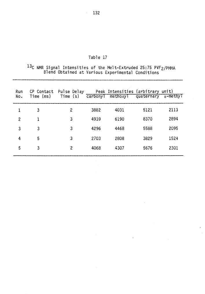
Run No.
1
2
3
4
5
132
Table 17
13c NMR Signal Intensities of the Melt-Extruded 25:75 PVF2/PMMA Blend Obtained at Various Experimental Conditions
CP Contact Pulse Delay Peak Intensities (arbitrary unit) Time (ms) Time Cs) car6onyl metlioxyl quaternary a-metny I
3 2 3882 4031 5121 2113
1 3 4939 6190 8370 2894
3 3 4296 4468 5588 2095
5 3 2703 2808 3829 1524
3 2 4068 4307 5676 2301

133
Table 18
Residual NMR Signal Intensities of PMMA in the 25:75 PVF2/PMMA Melt-Extruded Blend, Calculated from the CP Spectra with Various
Contact Times
CP Contact Time (ms)
1
3
5
Residual 13c NMR Peak Intensities (%) carbonyl methoxyl quaternary a-methyl
68
63
52
59
50
60
68
54
45
77
70
60
Pulse delay time= 3 seconds

134
Figure 14. DD-MAS-CP 15.0 MHz C-13 NMR Spectra of PMMA Obtained at Various Contact Times.

135
CP Time
0.02ms ~ " ... 4 ____,..-
----~ -0.05ms
O.lms
0.2ms
O.Jms
0.6ms
1.0ms
2.0ms
J.Oms
4.0ms
6.0ms
-"'-- 8.0ms ~ ....... ...,.... ..._,,._ l/J/PVF2/PMMA
- ·-Figure 15. DD-MAS-CP 15.0 MHz C-13 NMR Spectra of the Melt-Extruded
25:75 PVF2/PMMA Blend Obtained at Various Contact Times:

! '
1 I_ --nlmax
-1
-2
1.
CARBONYL CARBON
2. J. CP Time (ms)
4.
H -1/slope=Tlt
5, 6. -
•
7. a•.~.
Figure 16. 13c NMR Signal Intensity for the Carbonyl Carbon of PMMA in the Homopolymer and in the Melt-Extruded 25:75 PVF2/PMMA Blend as a Function of Contact Time.
vJ CJ)

137
Table 19
PMMA C-13 Resolved Proton T1R Values of the Homopolymer and the PVF2/PMMA Blends
Proton T1g Values {ms) Calculated From
Samples car5ony1 metlioxy1 quaternary
PMMA 9.1 9.4 8.6
25:75 extruded 6.7 5.4 5.8 PVF2/PMMA blend
50:50 extruded 3.8 3.9 3.7 PVF2/PMMA blend
a-methy1
8.3
5.9
3.4

Samples
25:75 Extruded PVF2/PMMA Blend
50:50 Ex·truded PVF2/PMMA Blend
Table 20
Residual NMR Signal Intensities of PMMA in Two Melt-Extruded PVF2/PMMA Blends as an Effect of Sample Aging
Sample History Residual 13c NMR Peak Intensities (%) CP Contact (days after
Time (ms) blending) carbony1 methoxy1 quaternary a-methyT
3 1 52a 45a 47a 66a
3 34 63b sob 54b 1ob
3 118 56 47 61 75
* 118 62-A· 58* 71* 85* ·-
3 1 35a 2aa 37a s1a
3 218 47 32 46 64
* 218 70* 50* 74* 111*
* calculated from Mo*, the theoretical maximum magnetization attainable, when T1pH>>CP contact time»TcH
a. results of Table 13 b. results of Table 18
........ w ():)

139
values obtained from four 13c resonance peaks show some scatter (which
should be the same) due to the limited number of spectra (data points)
used in determining the Tip's and the limited sensitivity of the NMR
instrument. However, it is obvious that proton's T1p values are
different among the three samples.
The theoretical maximum magnetization of PMMA attainable in the CP ·
process in the homopolyme·r and the two blends was calculated for the H
Tip's using Equation (91). Residual NMR signal intensitites of PMMA in
the two blends calculated from the theoretical maximum magnetization are
given in Table 20. The table also lists the results calculated from a
CP contact time of 3 ms of. the same experiments as wel 1 as results of
the previous experiments on the s~me samples.
IV. DISCUSSION
A. Shifts of NMR Frequencies
As a result of the interactions between PVF2 and the other polymers
in the miscible blends, one might expect some shifting of various NMR
peaks away from their initial frequencies similar to what is observed in
FT-IR studies (165). However, due to the inherent resolution limitation
of NMR instruments in addition to the decreased sensitivity obtained
with.the miscible blends (signal attenuations), no significant NMR
chemical shifts were induced by blending. Mixed tacticities in the
non-PVF2 polymers also contributed to this lack of resolution.
B. NMR Signal Attenuations and Degr~es of Intermixing
From Tables 13, 14,15, it is apparent that most of the data for the

140
magnitudes of 13c signal atte~uations of PMMA, PVAc and PVME in the
blends with PVF2 were in very good agreement with the melting point
depressions of PVF2 in the blends. The method of melting point
depression has become widely accepted as an indicator of the degree of
blend miscibility when semicrystal~ine polyners are involved. For
example, this number can be directly related to the polymer-polymer free
energy interaction parameter as discussed in Chapter I (section
III.B.6). Clearly, a macroscopic, thermodynamic observation is all that
may be obtained in this case. In comparison, NMR signal attenuations of
any polymer blended with PVF2 as observed in the present work indicate
to some extent spatial proximity of that polymer with PVF2. It will be
shown below that intermolecular distances for 13c-19F dipolar coupl~ng
as observed by the present method was in the range of 3 to 4A. Among
the blends which were examined, except for the DMF cast PVF2/PVAC blends
with thermal treatment, both the methods of melting point depression and
NMR signal attenuations indeed provided consistent indications cf the
extent of compatibility from very different experimental approaches.
The data in Tables 13, 14 and 15 for the three series of blends are
discussed individually in the next three sections.
1. PVF2/PMMA Blends
Without any thermal treatment, MEK was a better common solvent
for blending than was DMF; attenuation of 13c resonances was nil in the
latter case. Although the mixtures of PVF2 and PMMA in DMF were clear,
the dried samples of al 1 composi ti ens cast from DMF were totally
immiscible as measured by both the NMR and DSC studies.

141
Melting-and-quenching the blends appeared to improve miscibility
according to the NMR work; PVF2 crystallinity was undetectable by DSC in
some of these samples. The differences in NMR signal attenuations
between the MEK-blended and the DMF-blended samples with the same
composition became sma 11 er after the melting and quenching process.
However, the miscibility of both wa.s indicated to remain poorer than
that of the melt-extruded blends having the same composition.
For solvent-blended samples in the composition ranges studied, it
was observed that the higher the PVF2 content, the greater the
amount of PMMA 13c signal attenuation. For the melt-extruded blends,
the one with medium PVF2 content (50% by weight) showed the highest
degree of 13c signal loss.
The significant disparity in miscibility between the DMF and MEK
cast films could result from the difference in rates of solvent
evaporation. For the 2% solutions, it was observed that DMF evaporated
about ten times mere slowly than MEK. This is consistent with a
better and more complete crystalliaztion as well as a poorer
miscibility of the DMF cast films.
The polymorphic nature of the PVF2 crystallinity may also in part
explain the results. The morphology of PVF2 homopolymers has been
extensively investigated (177). The effect of sample history on the
morphology of PVF2 is summarized in Figure 17 {178). It was repcrted
that crystallization from DMF resulted in a y-phase, while
crystallization from melt and from cyclohexane (which, like MEK, is a
saturated aliphatic ketone) usually resulted in an a-phase. Therefore,

.,4? !. .....
HIGH T .----~ !POSSIBLY AT HIGHT?) -----Hl_G_H_P __ _, MELT -----------:
~----<..'~-'=' HIGH P I
I- i;j J: (/) <!) <( - J: J: a.. I- ' <( "' <!l LLI z .J :J ~ <( (/) WO z a. z~
<(
"/1': I 4-f;t4. I
'(<;.. : 01' I
+19,. l ANNEALING AT HIGH T I
DRAWING AT LOW T UL TRAORAWING AT HIGH T
ANNEALING AT VERY HIGH P
I~ lw-za. I z J:
<( <!)
1~:i: 1'.j~ IOJ<!> I iii z Cll-1g
....._ _____ __, SOLUTiON 1---C-Y-CL_O_H_E_X_A_N_O-NE----' MCB/DMF,
CYCLOHEXANONE
Figure 17. Schematic Summary of Crystallization· and Interconversions of the Polymorphic Phases of PVF2 (178}. (T =temperature; P =pressure; E =electric field).

143
the MEK cast films are expected to have closer miscibility to the
melt-extruded blends than the DMF cast fi1ms.
Melting-and-quenching the solution cast films are likely to result
in the sar.1e crystal form as the me 1 t-extrus i en process. However, in the
former case, the driving force of miscibility would be
solely from diffusion. In contrast, in the latter case, molecular
diffusion in addition to mechanical force could result in better
homogeneity or miscibility of the blends. The difference in dependence
of PMMA 13c signal attenuation on the composition for the blends
prepared from the two methods may also result from the complicated
crystallization process of PVF2.
2. PVF2/PVAc Blends
For PVF2/PVAc blends, as for PVF2/PMMA blends,without any
thermal treatment, MEK appeared to be a better common solvent for
blending than DMF, although miscibility for the DMF cast PVF2/PVAc
samples was observed over a wide range of compositions. Compared to the
PFVz/PMMA blends made with the same common solvent, the PVF2/PVAc blends
made from both DMF and MEK solutions were found to have much better
mi sci bil i ty as indicated by both the NMR and DSC results shown in Tab 1 e
14. This better miscibility could be due to the slightly greater
interaction between PVF2 and PVAc than that between PVF2 and PMMA, as has been reported from melting point depression studies (171). It may
also result from the glass transition temperature of the PVF2/PVAc
blends (about or below room temperature) which is lower than that of
PVF2/PMMA blends (above room temperature) (171). For the DMf cast

144
samples, carbon-13 NMR signal attenuations of PVAc were found to pass
through a minimum as the PVF2 content was increased. The loss of
mi sci bil i ty at the higher PVF 2 content probab 1y was due to the higher
degrees of PVF2 crystallinity ir. those blends.
For the solvent (DMF and MEK) blended PVF2/PMMA samples, the degree
of intermixing was found to be enhanced after a melting-and-quenching
process, as evident from both the NMR and DSC studies. On the contrary,
the NMR studies of the solvent blended PVF2/PVAc samples revealed that a
process of high temperature (ca. 200°C) compression molding and
subsequent cooling to ambient temperature reversed the intimacy of the
mixing between the two polymers even though the melting point of PVF2
was practically unchanged with the process.
Although thermally induced phase separation, or the lower critical
solution temperature behavior (LCST) (Figure 4 shows an upper critical
solution temperature behavior (UCST)) has been observed in many blends
of PVF2, a cloud point due to reaching the LCST for the PVF2/PVAc blends
was not observed up to 350°C (169,171). The reasons for the absence of
LCST behavior were reported to be either from the enhanced phase
stability caused by the intense interaction between PVF2 and PVAc or due
to a close similarity of refractive indices of the two polymers (169).
The inconsistency between the NMR and DSC results for the mo1 ded
PVF2/PVAc samples can b~ partially understood by knowing that the
experimenta 1 probe size in this NMR stud·i es was about two orders saml 1 er
than those associated with the glass transition or light transparency
methods. It can be concluded that molding-and-cooling process is likely

145
to result in small scale modification of the crystals of PVF2 in the
PVFz/PVAc blends.
3. PVF2/PVME Blends
In Table 15, a summary of observations on the PVF2/PVME blends
is presented. Although both pure materia·ls dissolve readily in DMF the
cast films were concluded to be totally immiscible by both the NMR and
DSC results, confirming previously observed data of other
researchers (171}. The coincidence of signal intensities which are
enhanced rather than di mini shed by the DMF casting sequence and elevated
PVF2 melting point is especially noticeable in Table 15.
4. NMR Signal Attenuations of Individual Carbons
The nature of the mi sci bi 1 i ty of both the PVF 2/PMMA and the
PVF2/PVAc blends previously has been attributed to a weak intermolecular
'acid-base' association. In particular, an interaction was postulated
between tile acidic protons of PVF2 and the basic carbonyl groups in the
case of both PMMA and PVAc (165,171}. Knowing that the definition of
miscibility in these NMR experiments has to be confined to approaches of
dissimilar nuclei to within about 4A, it was expected that it might be
possible to observe differing extents of NMR peak attenuations for each
carbon. Depending on how much less than 4A the contact actually was on
the a'1erage, an estimate of the specificity of interatomic mixing could
be made.
From Table 13, for the PVFz/PMMA blends, there were four
resolvable NMR peaks in the spectra of PMMA; the methoxyl carbon which
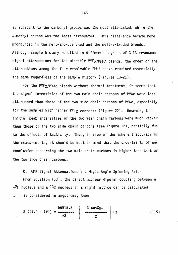
146
is adjacent to the carbonyl groups was the most attenuated, while the
a-methyl carbon was the least attenuated. This difference became more
pronounced in the melt-and-quenched and the melt-extruded blends.
Although sample history resulted in different degrees of C-13 resonance
signal attenuations for the miscible PVF2/PMMA blends, the order of the
attenuations among the four resolvable PMMA peaks remained essentially
the same regardless of the sample history (Figures 18-21).
For the PVF2/PVAc blends without thermal treatment, it seems that
the signal intensities of the two main chain carbons of PVAc were less
attenuated than those of the two side chain carbons of PVAc, especially
for the samples with higher PVF2 contents (Figure 22). However, the
initial peak intensities of the two main chain carbons were much weaker
than those of the two side chain carbons (see Figure 12), partially due
to the effects of tac ti city. Thus, in view of the inherent accuracy of
the measurements, it should be kept in mind that the un~ertainty of any
conclusion concerning the two main chain carbons is higher than that of
the two side chain carbons.
C. NMR Signal Attenuations ~nd Magic Angle Spinning Rates
From Equation (50), the direct nuclear dipolar coupling between a
19F nucleus and a 13c nucleus in a rigid lattice can be calculated.
If r is considered in angstroms, then
56815.2 3 cos2e-1 2 D(l3C - 19F) Hz ( 115)
r3 2

J47
100
-CHJ -C=O
I I
-C-~
I
H -OCHJ l:/J z fl::l 8 z H
~
PIVilVIA I MEK
Figure 18. % Residual C-13 Resonance Intensities of PMMA in the MEK-Cast PVF2/PMMA Blends.

148
PMMA I MEK I QUENCH
-C:.O I 1
-C-r -OCHJ
o~~~~--''--~~~--l~~~~---l'---~~~.......J
0 % PVF2 100
Figure i9. % Residual C-13 Resonance Intensities of PMMA in the MEK-Cast, Melted-and-Quenched PVF 2/PMMA Bl ends.
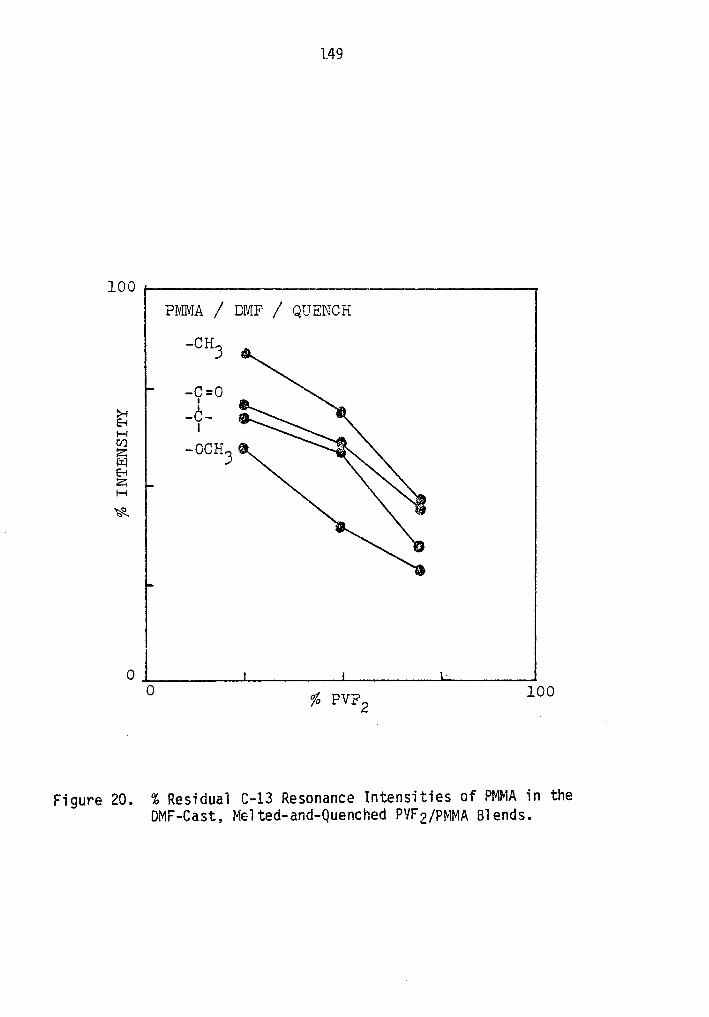
149
PMMA I DMF I QUENCH
-CHJ
-C=O I
-c-1
OCH - 3
% PVF2 100
Figure 20. % Residual C-13 Resonance Intensities of PMMA in the DMF-Cast, Melted-and-Quenched PVF2/PMMA Blends.

.1;50
EXTRUDED WITH PMMA
~ ~CHJ H ti) z J:i:l -9=0 8 z -6-H
I ~ -OCHJ
Figure 21. % Residual C-13 Resonance Intensities of PMMA in the Melt-Extruded PVF 2/PMMA Bl ends.

-CH-
-C;:O I
PVAc / DMF
Figure 22. % Residual C-13 Resonance Intensities of PVAc in the DMF-Cast PVF2/PVAc Blends.

i. e. 2 D = 56815.2
2 D = 7101.9
2 D = 2104.2
2 D = 887.7
152
3 ? cos~e-1
-----··----- Hz., if r=lA 2
3 cos2e-l ----------- Hz., if r=2A
2
3 cos2e-l ----------- Hz., if r=3A
2
3 cos2e..:1 ----------- Hz., if r=4A
2
The maximum value of D would be realized when the angular term within
the brackets is unity.
In looking at the influence of distance on dipolar coupling the
salient fact is that the MAS itself can decouple long range weak dipolar
interactions, with faster MAS decoupling only those of shorter range;
i.e., estimation of miscibility in this study is limited by the chosen
MAS rate. On the other hand, an investigation of NMR signal
attenuations of polymer blends containing PVF2 over a wide range of MAS
rates would generate an average concentration profile of the spatial
distribution of those 19F nuclei in the vicinity of any resolvable 13c
nucleus. Unfortunately, due to the limitations of our equipment, the
only comparison that could be made was at the spinning rates of 2.0 and
2.3 KHz. Some results for the melt-extruded PVF2/PMMA blends are shown
in Table 13. No significant spectral differences were seen at these two
spinning rates. Considering the inverse third power dependence of the
dipolar coupling on the internuclear distance, the expected effect is
only (2.3/2.0)l/3 = 1.048 in magnitude. Consequently, the results are

153
not surprising given the iimited frequency range. MAS rates as high as
15 KHz have been achieved using helium as the driving gas (63) which
suggests that if the NMR signal attenuations were compared at, e.g. the
MAS rates of 16 and 2 KHz, then a factor of 2 in the decoupling-distance
relationship might be achieved with an added gain in insight to the
understanding of the internuclear distance questions.
D. NMR Signal Attenuations and Relaxation Times
As discussed in Chapter I (section II.D.4), the technique of (13c-
1H) cross polarization is used not only to rapidly polarize carbon
magnetization (by ~T1H/T1c) but also to achieve greater total nuclear
magnetic alignment with the applied field than would otherwise be
possible. The cross polarization enhincement of 13c polarization at the *C C C
end of the CP contact is by a factor of M0 = YH/Yc ~ 4 M0 , where Mo is
the polarization which would be generated in H0 after waiting several
relaxation times, Tic. H
c However, this optimal enhancement of Mo can be
achieved only if Tip >> CP contact time >> TCH· If 13c nuclear spin
alignment varied with the composition of PVF2 polymer system, then
unfair comparisons of attenuation might result. An equivalent statement
would be that the 13c relaxations might begin at different spin
temperatures and attenuation calculations thus might be erroneous. H
Both the Tip and the TcH are modulated by molecular motion. It follows that average molecular mobility for a component in a pure
polymer and in a polymer blend (especially highly miscible ones) might
conceivably be different. Thus, while comparing the NMR signal
intensities from the CP spectra of a polymer and of its blends, these

154
relaxation parameters have to be considered for reasons given above. In
fact, any change of these relaxation times in itself is an indication of
the miscibility. The choice of CP time is especially important;
comparing NMR intensities of a polymer and those of its blends from CP
spectra in which the same contact time was specified could be misleading H
depending on T1p and TcH· Further investigation of this point was
required in order to have confidence in the results.
Tables 16 and 17 list the 13c NMR peak intensities of the PMMA and
the melt-extruded 25:75 PVF2/PMMA blend, respectively, obtained from
spectra in which three CP contact times and different pulse delays were
employed. Runs 1 and 5 were carried out at exactly the same conditions
to show the reproducibility of the experiments. Run 3 used the same CP
contact time as runs 1 and 5 but employed a longer pulse delay time.
The results show that for both the PMMA neat and the blends, 3 seconds
of pulse delay time was certainly long enough to assure the full
repolarization of the protons between the scans.
From Tables 16 and 17, it is apparent that the spin-locked
magnetization relaxed faster in the blends than in the PMMA homopolymer ( • T H ) 1.e. •lp is shorter in the blend than in the homopolymer. The
CP contact time used in all the examples in this study for the PMMA
and its blends was 3ms, which is obviously not the optimum for all
systems investigated. The residual NMR signal intensities of PMMA in
the 25:75 melt- extruded PVF2/PMMA blend were calculated from Tables 16
and 17 for the CP spectra obtained at various CP contact times; the
results are shown in Table 18.

155
Further investigation was done by studying PMMA as well as the
melt-extruded 25:75 and 50:50 PVF2/PMMA blends at twelve different
contact times for each (Figures 14 and 15). Averaged proton Tip values
of the three samples resolved from carbon-13 CP spectra showed a
decrease from 8.9 ms to 6.0 ms to 3.7 ms as the PVF2 content was
increased from Oto 50 wt. % (Table 19). This is consistent with the
results of NMR signal attenuations (Tables 13 and 20) as well as the
glass transition behavior of the PVF2/PMMA blends reported in the
literature (171).
The contri bu ti ons of the NMR si gna 1 attenuati ans of PMMA in the tw.o
blends due to the modifications of proton Tlp values were estimated by
comparing the theoretical maximum CP peak intensities of pure PMMA and
the two blends {Table 20). This exploration showed that among the three
resolvable peaks of the highest intensities, with a contact time of 3
ms, 14-26% and 26-52% of the attenuations resulted from the shorter
proton's Tip's in the 25:75 and 50:50 PVF2/PMMA blends, respectively.
The results of NMR signal attenuations calculated from the theoretical
CP magnetization showed insignificant differences between the two
blends. This indicated that the degrees of intermixing were· about the
same between PMMA and PVF2 in the two blends. Nonetheless, proton Tlp values indicated that there was a stronger dynamic interaction between
the two polymers in the amorphous region of the 50:50 PVF2/PMMA blend
than in the 25:75 PVF2/PMMA blend.
It is c'iear that the severity of attenuation of the C-13 resonance
intensit·ies of PMMA in the blend as calculated from CP spectra can be

156
different for different contact times. However, among the four
resolvable peaks of the PMMA in the two melt-extruded blends, the
methoxyl carbon remains the most atter:uated and the a:-methyl carbon the
least attenuated regardless of the contact time. This point can be
elaborated by referring to Figures 14 and 15. In Figure 14, for the
pure PMMA, the peak intensity of the methoxyl carbon is greater than
that of the quaternary carbon regardless of the contact times. The
opposite trend between the peak intensities of these two carbons in the
blends can be seen in Figure 15.
E. NMR Signal Attenuations and Effect of Aging
When compared to the results on the freshly prepared samples {Table
131 a loss in magnitude of the attenuations of the C-13 resonance
intensities was observed· over time. For the same melt-extruded 25:75
and 50:50 P'IF2/PMMA blends discussed above in the variable contact time
studies {Tables 16-18) and in the T1pH studies, a significant drift
toward the hornopolymer signal intensities was observed. The discrepancy
of NMR signal attenuations for .the two blends obtained at from various
experiments is summarized in Table 20. This descrepancy might
conceivably be due to unknown experimental errors involving changes in
instrument response. However, perhaps the aging process of
the blends is more likely in the cause.
F. NMR Signal Intensities and Number of Accumulations
One of the assumptions in this study is that the NMR signal
intensities are directly proportional to the number of total

157
accumulations for each sample. However, when a iarge number of scans
are stored using only time domain accumulations, considerable
deterioration of the accumu1 ati on efficiency may take pl ace because of
the limited computer bit number. The JEOL-60Q instrument employed a
technique of progressive decrement of the A to D converter bit number in
order to avoid data overflow. This means that the dynamic range of the
spectra was thereby reduced, which would make· the assumption of S/N less
reliable, especially for the weak peaks. Thus, to avoid this problem,
all the spectra of this study were carried out at conditions such that
the final A to D converter bit number remained at 5 bits or more. Table
21 gives 13c NMR signal intensities of PMMA obtained at various number
of accumulations. The table shows that with our experimental conditons,
the assumptions concerning S/N remained effective.
V. CONCLUSIONS
From the results of this chapter, the following conclusions have
been reached.
1. Solid state 13c NMR is able to probe the-miscibility of the
polymer blends of PVF2. Degrees of molecular intermixing in the blends
were reflected through the 13c NMR signal attenuations. These
attenuations are mainly due to 13c-19F intermolecular di polar
interactions, which were not decoupled.
2. Molecular level indications of the proximity in the blends were
observed in this NMR study. The experimental probe size, or the
resolution of the intimacy of mixing between the two constituent

158
Table 21
13c NMR Signal Intensities of PMMA Obtained at Various Number of Accumulations
Number of Word Final AD 13c Peak Intensities Accumulations Length Converter . (arbitrary unit)
(bits) (bits} car5onyl me{fioxy I quaternary a-mettiy I
800 16 8 3565x28 476lx28 5844x28 1882x28
1600 16 7 3488x29 5095x29 5323x29 1730x29
3200 16 6 3468x210 4805x210 5592x210 173lx210
6400 16 5 3446x211 4732x211 5787x211 1852x211

159
polymers in the blends, was estimated to be in the range of 3 to 4
angstroms. Beyond this range, a MAS rate of 2 KHz reduced any si gna 1
attenuation of l9f on 13c nuclei. Various degrees of NMR signal
attenuations among the individual chemically different carbons of a
polymer support a postulation of weak intermolecular 'acid-base'
association between the acidic protons of PVF2 and the basic carbonyl
groups in the case of both the PMMA and the PVAc blends. For the
miscible blends, the· order of the attenuations among individual carbons
of either the PVF 2/PMMA or the PVF2/PVAc system remained es sen ti ally
unchanged regardless of their compositions and sample hi stroy as \.'1ell as
the NMR experimental parameters.
3. Results of 13c NMR signal attenuations revealed that with the
same sample history, PVAc is more miscible with PVF2 than is PMMA, ~'lhile
PVME is immiscible with PVF2. This order is consistent with the
conclusions of thermodynamic studies reported in the literature. In
this study, the results of 13c NMR signal attenuations were, in general,
in good agreement with the melting point depression of PVF2 in the
blends. Exceptions were observed for the DMF-cast PVF2/PVAc blends
having thermal treatment. This disparity is likely to be due to the
significantly different experimental probe sizes of the two techniques.
4. It has been well recognized that PVF2 forms miscible blends
with both PMMA and PVAc. However, from this solid state 13C NMR
studies, the methods of sample preparation and thermal treatment were
found to play a significant role in determining the miscibility. The
crystallization and interconversions of the polymorphic phases of PVF2

160
are likely to be an important factors and reflect the effect of sample
history.
5. Although the 13c-19F intermolecu1ar dipolar interactions were
concluded to be the main source of the 13C signal attenuations of the
blends, relaxation times (proton's Tip's in particular) could also
contribute to the attenuations. The modifications of proton Tip's are
more obvious in the highly miscible blends. The changes in themselves
are indications of miscibility.
6. With the experimental conditions of this study, deterioration
in the accumulation efficiency due to the progressive decrement of the
dynamic range was not a factor for the 13c NMR signal attenuations of
the blend.
7. The aged melt-extruded PVF2/PMMA blends showed less degrees of
13c NMR signal attenuations than the freshly prepared samples. This
discrepancy is probably due to the aging process of the blends.
8. No significant shifts of NMR frequencies induced by blending
were observed. This may be due to the inherent limitation in resolution
in solid state 13c NMR.
VI. FUTURE WORK
All the NMR experiments of this study were carried out at room
temperature in an instrument whose dipolar decoupling capability is
limited only to the protons. Some questions, though further
investigation on them were desired, could not be answered. Moreover,
the extension of this method of compatibility studies beyond 19F might

161
not be possible with the present instrumental capability.
In view of the upgrading of the present instrument, namely, the
variable temperature capability (VT-MAS (179,i80}}, in the very near
future, two aspects are recommended for future work as discussed below.
Another aspect which requires the capability of simultaneous dipolar
decouplings of both protons and fluorine-19 nuclei is also recommended
below.
A. Variable Temperature Studies
In this NMR study of polymer blends, sample history was found to
be very important in determining the compatibility. Although the
effects of thermal treatments on the polymer blend compatibility have
been studied, all the spectra were obtained at room temperature. With
the variable temperature capability, questions left unanswered in this
study can be further investigated. One example is the possible small
scale phase separation due to the LCST behavior of the PVF2/PVAc blends.
B. Compatibility Studies Through Heteronuclei Other Than rluorine-19
This compatibility study of polymer blends through intermolecular
heteronuc1ear d·ipolar interactions should be extensible to nuclei other
than fluorine-19. In terms of commercial organic polymers, chlorine is
a possible candidate. However, dipolar interactions due to chlorine
nuclei are usually negligible for solid polymers above their glass
transition temperature (84}. This is due to the self-decoupling induced
by effective quadrupolar relaxations in these systems. With the VT-MAS
capability, compatibility studies through intermolecular 13c-35C1 and

162
13c-37Cl dipolar interactions a~ a temperature well below the glass
transition of a polymer blend might be possible.
C. Compatibility Studies by Varying Heteronuclear Dipolar Decoupling Power
In the previous section, it was suggested that an ivestigation of
13c NMR signal attenuations of polymer blends containing PVF2 over a
wide range of MAS rates would generate an average concentration profile
of the spatial distribution of 19F nuclei that are in the vicinity of
the resolvable 13c nucleus. Besides the experimental difficulty in
achieving high MAS rates, low MAS rates could generate complex spinning
sidebands. The sidebands would make the quantitative treatment of the
spectra more complicated. An alternative approach to the variable MAS
rates could be achieved by simultaneously decoupling fluorine-19 nucleus
in addition to the protons. With a fixed rate of ca. 2 KHz, varying the
19F decoupling power might reveal the spatial distribution of 19F nuclei
within 3 to 4 angstroms of any resolvable 13C nucleus of a polymer in a
blend with PVF2.

1.
2.
3.
4.
5.
6.
7.
8.
9.
10.
11.
12.
13.
14.
15.
Literature Cited
N.A.J. Platzer, Ed., "Multicomponent Polymer Systems 11 , Adv. Chem. Ser., 99, ACS, Washington, D.C., 1971.
N.A.J. Platzer, Ed., "Copolymers, Polyblends, and Composites", Adv. Chem. Ser., 142, ACS, Washington, D.C., 1975.
S. L. Aggarwal, Ed., "Block Copolymers 11 , Plenum Press, New York, 1970.
A. Noshay and J. E. McGrath, 11 Block Copolymers: Overview and Critical Survey 11 , Academic Press, New York, 1977.
O. Olagoke, L. M. Robeson and M. T. Shaw, "Polymer-Polymer Mi sci bi 1 i ty", Academic Press, New York, 1977.
D. R. Paul and S. Newman, Ed., "Polymer Blends 11 , Academic Press, New York, 1978.
F. A. Bovey, 11 Encyclopedia of Polymer Science and Technology", N. M. Bikales, Ed., Wiley-Interscience, New York, 1968, Vol. 9, pp. 356-396.
I. Ya S1 onim and A. N. Lyubimov, "The NMR of Polymers 11 , Plenum Press, New York, 1970.
P. Diehl 1 E. Fluck and R. Kosfeld, Ed., "NMR Basic Principles and Progress 11 , Vol. 4: Nature and Synthetic High Polymers, Springer-Verlag, Berlin, 1971.
F. A. Bovey, "High Resolution NMR of Macromolecules 11 , Academic Press, New York, 1972.
E. M. Purcell, H.·C. Torrey and R. V. Pounds, Phys. Rev., 69, 37, 1946.
F. Block, W. M. Hansen and M. E. Packard, Phys. Rev., 69, 127, 1946.
T. C. Farrar and E. D. Becker, "Pulse and Fourier Transform NMR: Introduction to Theory and Methods 11 , Academic Press, New York, 1971.
K. Mullen and P. S. Pregosin, 11 Fourier Transform NMR Techniques -A Practical Approach", Academic Press, New York, 1976.
D. Shaw, "Fourier Transform NMR Spectroscopy 11 , Elsevier, Amsterdam, 1976.
163

16.
17.
18 ~
19.
20.
21.
22.
23.
164
C. Brevard and P. Granger, "Handbook of High Resolution Multinuclear NMR 11 , W·iley-Interscience, New York, 1981.
J.B. Stothers, 11 Carbon-13 NMR Spectroscopy 11 , Academic Press, New York, 1972.
F. W. Wehrli and T. Wirthlin, "Interpretation of Carbon-13 NMR Spectra", Heyden, London, 1976.
E. Breitmaier and W. Voelter, 11 13C NMR Spectroscopy: Methods and App'lications in Organic Chemistry", 2nd. Ed., Verlag Chemie, Wei nheim, 1978.
R. J. Abraham and P. Loftus, "Proton and Carbon-13 NMR Spectroscopy: An Integrated Approach", Heyden, London, 1979.
G. C. Levy, R. L. Lichter and G. L. Nelson, "Carbon-13 Nuclear Magnetic Resonance Spectroscopy", 2nd Ed., Wiley-Interscience, New York, 1980.
J. Schaefer, "Topics in Carbon-13 NMR Spectroscopy", Vol. 1, G. C. Levy, Ed., Wiley-Interscience, t·~ew York, 1974, pp. 150-208.
W. M. Pasika, Ed.i 11 Carbon-13 NMR in Polymer Science", ACS Symposium Series 03, ACS, Washington, D.C., 1979.
24. J.C. Randall, "Polymer Sequence Determination: Carbon-13 NMR Method", Academic Press, New York, 1977.
25. J. R. Lyerla, Jr., T. T. Horikawa and D. E. Johnson, J. Arn. Chem. Soc., 99, 2463, 1977.
26. G. C. Levy, P. L. Rinaldi, J. J. Dechter, D. E. Axelson and L. Mandel kern, "Polymer Characterization by ESR and NMR 11 , ACS Symposium Series, 142, A. E. Woodward and F. A. Bovay, Ed., ACS, Washington, D.C., 1980, pp. 119-146.
27. W. P. Siichter, in Reference 9, pp. 209-231.
28. T. M. Connor, in Reference 9, pp. 247-270.
29. V. T. McBriety, Polymer, 15, 503, 1974.
30. V. T. McBriety and D. c. Douglass, J. of Polym. Sci.: Macromolecular Reviews, 16, 295, 1981.
31. 1. Ya Slonim, 11The Ageing and Stabilization of Polymers 11 ,
A. s. Kuz'minskii, Ed., Elsevier, Amsterdam, 1971, pp. 244-262.

165
32. M. Mehring, "High Resoiution NMR Spectroscopy in Solids", Springer-Verlag, Berlin, 1976.
33. 11 Pul se Nuclear Magnetic Resonance in Sol i ds 11 , Faraday Symposia of the Chemical Society, No. 13, The Chemical Society, London, 1978.
34. "Nuclear Magnetic Resonance Spectroscopy in Solids 11 , The Royal Society, London, 1981; also published as Phil. Trans. Roy. Soc. London, A299, pp. 475-686, 1981.
35. G. Scheler, U. Haubenreisser and H. Rosenberger, J. Magn. Reson., 44' 134, 1981.
36. C. S. Yannoni, Acc. Chem~ Res., 15, 201, 1982.
37. Chem. Eng. News, October 16, 1978, p. 23.
38. J. Schaefer, E. 0. Stejskal and R. Buchdahl, Macromolecules, 10, 384, 1977.
39. J. R. Lyerla, 11 Contemporary Topics in Polymer Science 11 , Vol. 3, M. Shen, Ed., Plenum Press, New York, 1979, pp. 143-213.
40. R. K. Harris, K. J. Packer and B. J. Say, Makromol. Chem., Suppl. 4, 117, 1981.
41. H. A. Resing, A. N. Garraway, D. C. Weber, J. Ferraris and D. Slotfeldt-Ellingsen, Pure & Appl. Chem., 54, 595, 1982.
42. J. A. Pople, W. G. Schneider and H. J. Berstein, "High-Resolution Nuclear Magnetic Resonance", McGraw-Hil 1, New York, 1959.
43. A. Abragam, 11The Principles of Nuclear Magnetism 11 , Clarendon Press, Oxford, 1961.
44. C. P. Slichter, "Principles of Magnetic Resonance 11 , 2nd. Ed., Springer-Verlag, Berlin, 1978.
45. M. L. Martin~ G. J. Martin and J. -J. Delpuech, 11 Practical NMR Spectroscopy' , Heyden, London, 1980. .
46. E. Fukushima and S.B.W. Roeder, "Experimental Pulse NMR: A Nuts and Bolts Approach 11 , Addison-Wesley, London, 1981.
47. Reference 45, pp. 411-413.
48. Reference 13, pp. 8-15.
49. F. Bloch, Phys. Rev., 70, 460, 1946.

166
50. F. Bloch, W.W. Hanson and M. Packard, Phys. Rev., 70, 474, 1946.
51. E. L. Hahn, Phys. Rev., 80, 580, 1950.
52. J. W. Cooper, Comput. Chem., l, 55, 1976.
53. Reference 43, Chapter 4.
54. J. Schaefer, Macromolecules, 6, 882, 1973.
55. K. Yokota, A. Abe, S. Hosaka, I. Sakai and H. Saito, Macromolecules, 11, 95, 1978.
56. A. A. Jones, G. L. Robinson and F. E. Gerr, in Reference 23, pp. 271-290.
57. Reference 45, p. 17.
58. J. W. Emsley and J.C. Lindon, 11 NMR Spectroscopy Using Liquid Crystal Solvents", Pergamon Press, Oxford, 1975.
59. J. H. Noggle and R. E. Schirmer, "The Nuclear Overhauser Effects -Chemical Applications", Academic Press, New York, 1971.
60. B. C. Gerstein, Anal. Chem., 55, 781A, 1983.
61. E. R. Andrew~ "Progress in Nuclear Magnetic Resonance Spectroscopy , Vol. 8, J. W. Emsley, J. Feeney and L. H. Sutcliffe, Ed., Pergamon Press, New York, 1972, pp. 1-39.
62. E. R. Andrew, in Reference 34, pp. 505-520.
63. K. W. Zilm, D. W. Alderman and D. M. Grant, J. Magn. Reson., 30, 563' 1978.
64. I. J. Lowe, Phys. Rev. Lett., 2, 285, 1959.
65. E. R. Andrew, L. F. Farnell and T. D. Gledhill, Phys. Rev. Lett., 19' 6' 1967.
66. E. R. Andrew and L. F. Farnell, Mclee. Phys., 15, 157, 1968.
67. A. C. Cunningham and S. M. Day, Phys. Rev., 152, 287, 1966.
68. U. Haeberlen, 11 High Resolution NMR in Solids: Selective Averaging 11 , Adv. Magn. Reson., Suppl. 1, Academic Press, New York, 1976.
69. J. Herzfeld and A. E. Berger, J. Chem. Phys., 73, 6021, 1980.

167
70. L. W. Jelinski, Macromoiecules, 14, 1341, 1981.
71. S. R. Hartmann and E. L. Hahn, Phys. R~v., 128, 2042, 1962.
72. J. P. Jessen, P. Meakin and G. Kneissel, J. Am. Chem. Soc., 95, 618, 1973.
73. J. S. Waugh, L. M. Huber and U. haeberlen, Phys. Rev. Lett., 20, 180' 1968.
74. P. Mansfield, J. Phys. C: Solid St. Phys., 4, 1444, 1971.
75. W. -K. Rhim, D. D. Elleman and R. W. Vaughan, J. Chem. Phys., 58, 1772, 1973.
76. D. P. Burum and W. -K. Rhim, J. Chem. Phys., 71, 944, 1979.
77. U. Haeberlen and J. S. Waugh, Phys. Rev., 175, 453, 1968.
78. Reference 44, Chapter 3.
79. H. Kessemeier and R. E. Norberg, Phys. Rev., 155, 321, 1967.
80. D. L. VanderHart, W. L. Earl and G. N. Garraway, J. Magn. Reson., 44' 361, 1981.
81. W. P. Aue, 0. J. Ruben and R. G. Griffin, J. Magn. Reson., 43, 472' 1981.
82. W. T. Dixon, J. Magn. Reson., 44, 220, 1981.
83. W. P. Rothwell and J. S. Waugh, J. Chem. Phys., 74, 2721, 1981.
84. W.W. Fleming, C. A. Fyfe, J. R. Lyerla, H. Vanni, and C. S. Yannoni, Macromolecules, 13, 460, 1980.
85. A. Pines, M. G. Gibby and J. S. Waugh, J. Chem. Phys., 59, 569, 1973.
86. s. R. Hartmann and E. L. Hahn, Phys. Rev., 128, 2042' 1962.
87. E. o. Stejskal and J. Schaefer, J. Magn. Reson., 18, 560, 1975.
88. E. O. Stejskal, J. Schaefer and T. R. Steger, in Reference 33, pp. 56-62.
89. s. J. Opella and M. H. Frey, J. Am. Chem. Soc., 101, 5854' 1979.
90. D. A. Torchia, J. Magn. Reson., 30, 613, 1978.

168
91. Reference 2. Preface
92. M. Steinberg, L. E. LuKacka, P. Colombo and B. Manowitz, in Reference 1, pp. 547-561.
93. P. J. Flory, "Principles of Polymer Chemistry", Cornell University Press, Cornell, 1953.
94. O. Olabishi, J. Chem. Ed., 58, 944, 1981.
95. R. Koningsveld, L. A. Kleintjens and H. M. Schoffeleers, Pure Appl. Chem., 39, 1, 1974.
96. A. J. Yu, i!1 Reference 1, pp. 2-14.
97. P. Gl ansdorff and I. Pri gogi ne, 11Thermodynami c Theory of Structure, Stability and Fluctuations", Wiley-Interscience, London, 1971.
98. J. H. Hildebrand and R. L. Scott, "The So 1ubi1 i ty of Non-Electrolytes", Reinhold, 1950.
99. L. Bohn, Rubber Chern. Technol., 41, 495, 1968.
100. T. L. Hill, "An Introduction to Stastical Thermodynamics", Addi son-\Jesl ey, Reading, 1960.
101. P. J. Flory, J. Chem. Phys., 9, 660, 1941.
102. P. J. Flory, J. Chem. Phys. , 10, 51, 1942.
103. M. L. Huggins, J. Chem. Phys., 9, 440, 1941.
104. M. L. Huggins, J. Phys. Chem., 46, 151, 1942.
105. P. J. Flory, J. Arn. Chem. Soc. , 87, 1833, 1965 •
106. D. Patterson, Macromolecules, 2, 672~ 1969.
107. D. J. Meier, J. Polym. Sci., Part C, 26, 81, 1969.
108. D. J. Meier, Polym. Prepr., ~~. Chem. Soc., Div. Polym. Chem., 11, 400' 1970.
109. S. Krause, J. Polym. Sci., Part A-2, 7, 249, 1969.
110. S. Krause, Macromolecules, 3, 84, 1970.
111. D. F. Leary and M. C. Williams, J. Polym. sci., Part B, 8, 335, 1970.

169
112. D. F. Leary and M. c. Wil 1 i ams, J. Polym. Sci., Polym. Phys. Ed., 11, 345' 1973.
113. D. F. Leary and M. c. Wi 11 i ams, J. Polym. Sci., Po lym. Phys. Ed., 12' 265' 1974.
114. D. J. Meier, Polym. Prepr., Am. Chem. Soc., Div. Polym. Chem., 15' 171, 1974.
115. 0. S. Kaplan, J. Appl. Po1ym. Sci., 20, 2615, 1976.
116. R. W. Smith and J. C. Andries, Rubb. Chem. Tech., 47, 64, 1974.
117. M. Matsuo, C. Nozaki and Y. Jyo, Polym. Eng. Sci., 9, 197, 1969.
118. T. Nishi and T. T. Wang, Macromolecules, 8, 909, 1975.
119. T. K. Kwei, G.D. Patterson and T. T. Wang, Macromolecules, 9, 780' 1976.
120. V. J. McBrierty, D. C. Douglass and T. K. Kwei, Macromolecules, 11' 1265' 1978.
121. T. K. Kwei, T. Nishi and R. F. Roberts, Macromolecules, 7' 667' 1974.
122. T. Nishi , T. T. Wang and T. K. Kwei, Macromolecules, 8, 227' 1975.
123. T. Nishi , T. K. Kwei 1975.
and T. T. Wang, J. Appl. Phys., 46' 4157'
124. D. C. Douglass and V. T. McBriety, Macromolecules, 11, 766, 1978.
125. D. C. Douglass, Polym. Prepr. Am. Chem. Soc., Div. Polym. Chem., 20' 251, 1979.
126. J. E. Anderson and K. J. Liu, Macromolecules, 4, 260, 1971.
127. G. E. Wardell, V. J. McBriety and D. C. Douglass, J. Appl. Phys., 45, 3441, 1974.
128. R. A. Assink and G. L. Wilkes, Polym. Eng. Sci., 17, 606, 1976.
129. M. F. Froix and J. M. Pochan, J. Polym. Sci., Polym. Phys. Ed., 14' 1047' 1076.
130. R. A. Assink, J. Polym. Sci., Polym. Phys. Ed., 15, 59, 1977.
131. R. A. Assink, Macromolecules, 11, 1233, 1978.

170
132. D. J. Goldwasser, J. Polym. Sci., Polym. Phys. Ed., 17, 1464, 1979.
133. J. Schaefer, M. D. Sefcik, E. O. Stejskal, and R. A. McKay, Polym. Prepr., Am. Chem. Soc., Div. Polyru. Chem., 20, 247, 1979.
134. J. Schaefer, M. D. Sefcik, E. O. Stejskal, and R. A. McKay, Macromolecules, 14' 188' 1981.
135. E. o. Stejskal, J. Schaefer, M. D. Sefcik, and R. A. McKay, Macromolecules, 14' 275' 1981.
136. L. W. Jelinski, F. C. Schilling and F. A. Bovay, Macromolecules, 14' 581, 1981.
137. M. Morton, Ed., "Rubber Technology", 2nd Ed., Van Nostrand Reinhold, New York, 1973.
138. D. A. Meyer, in Reference 137, pp. 440-458.
139. W. R. Hendricks and R. J. Enders, in Reference 137, pp. 515-533.
140. M. Shen and D. H. Kaelble, J. Polym. Sci., Polym. Lett. Ed., 8, 149, 1970.
141. E. Helfand, Macromolecules, 8, 552, 1975.
142. G. Kraus and K. W. Rollmann, J. Polym. Sci., Polym. Phys. Ed., 14~ 1133' 1976.
143. P. L. Kumler and S. E. Keinath, Polym. Eng. Sci., 17, 613, 1977.
144. U. Bianchi, E. Pedemonte and A. Turturro, Polymer, 11, 268, 1970.
145. B. Morese-Seguela, M. St-Jacques, J. M. Renaud and J. Prud'homme, Macromolecules, 13, 100, 1980.
146. G. L. Wilkes and R. Wildnauer, J. Appl. Phys., 46, 4148, 1975.
147 •. G. L. Wilkes and J. A. Emerson, J. Appl. Phys., 47, 4261, 1976.
148. Reference 10, pp. 125-126 and pp. 226-229.
149. FAFT 70 Floppy Disk FG/BG Program, Intruction Manual, JEOL. LTD.
150. T. Hashimoto, K. Nagatoshi, A. Todo, H. Hasegawa and H. Kawai, Macromolecules, 7, 364, 1974.
171
151. P. M. Toporowski and J. E. L. Rooves, J. Polym. Sci., Polym. Chem. Ed., 14, 2233, 1976.
152. Reference 4, pp. 198-203.
153. J. Brandrup and E. H. Immergnt! Ed., "Polymer Handbook", 2nd Ed., Wiley-Interscience, New York, 1975.
154. J. Schaeffer, E. 0. Stejskal and R. Buchdahl, J. Macromol. Sci., Phys., B 13, 665, 1977.
155. Reference 4, pp. 371-379.
156. H. Morawetz, F. Amrani, Macromolecules, 11, 281, 1978.
157. C. W. Frank, M. A. Gashgari, Macromolecules, 12! 163, 1979.
158. T. C. Ward and T. S. Lin, AIChE Meeting, Nov. 1982, and ACS Adv. Chem. Ser., in press.
159. T. S. Lin and T. C. Ward) Polym. Prep., Am. Chem. Soc., Div. Polym. Chem., 24, Sept. 1983, in press.
160. F. F. Koblitz, R. G. Petrella, A. A. Dukert and A. Christbfas, U. S. Patent, 3,253,060, 1966.
161. C. H. Miller, Jr., U. S. Patent, 3,458,391, 1969.
162. J. M. Schmitt, U. S. Patent, 3,459,834, 1969.
163.
164.
165.
166.
167.
168.
169.
J. S. Noland, N. N.-C. Hsu, R. Saxon and J. M. Schmitt, in Reference 1, pp. 15-28.
D. R. Paul and J. 0. Altamirano, in Reference 2, pp. 371-385.
M. M. Colemann, J. Zarian, D. F. Varnell and P. C. Painter, J. Polym. Sci., Po1ym. Lett. Ed., 15, 745, 1977.
T. K. Kwei, H. L. Frisch, W. Radigan and S. Vogel, Macromolecules, 10' 157 ' 1977.
F. A. Bovey, F. C. Schilling, T. K. Kwei and H. L. Frisch, Macromolecules, 10, 559, 1977.
D. C. Wdhrmund, R. E. Bernstein, J. W. Barlow and D. R. Paul, Polym. Eng. Sci., 18, 677, 1978.
R. E. Bernstein, 0. R. Paul and J. W. Barlow, Polym. Eng. Sci., 18, 683' 1978.

172
170. R. E. Bernstein, D. C. Wahrmund, J. W. Barlow and D.R. Paul., Polym. Eng. Sci., 18, 1220, 1978. ·
171. D. R. Paul, J. W. Barlow, R. E. Bernstein and D. C. Wahrmund, Polym. Eng. Sci., 18, 1225, 1978.
172. I. R. Peat and W. F. Reynolds, Tetrahedron Lett., 14, 1359, 1972.
173. T. K~ Wu and D. W. Ovenall, Macromolecules, 7, 776, 1974.
174. L. F. Johnson, F. Heatly and F. A. Bovey, Macromolecules, 3, 175, 1970.
175. J.B. Lando, H. G. Olf and A. Peterlin, J. Polym. Sci., Part A-1, 4, 941, 1966.
176. R. Hasegawa, Y. Takahashi, Y. Chatani and H. Tadokoro, Poiym. J., 3' 600' 1972.
177. A. J. Lovinger, "Developments in Crystalline Polymers-1 11 , D. C. Bassett, Ed., Applied Science, London, 1982, pp. 195-273.
178. Reference 177, p. 216.
179. W. W. Fleming, C. A. Fyfe, R. D. Kendrick, J. R. Lyerla, H. Vanni and C. S. Yannoni, 11 Polymer Characterization by ESR and NMR 11 , ACS Symposium Series, 142, A. E. Woodward and F. A. Bovay, Ed., ACS, Washington, D.C., 1980, pp. 193-217.
180. J. R. Lyerla and C. S. Yannoni, Acc. Chem. Res., 15, 208, 1982.

The vita has been removed from the scanned document

Applications of High Resolution Solid State Carbon-13 NMR to the Study of Multicomponent Polymer Systems
by
Tso-Shen Lin
(ABSTRACT)
The technique of high resolution solid state carbon-13 NMR,
achieved with magic angle spinning (MAS) and high power 13c-1H dipolar
decoupling and cross polarization, was applied to a number of multi-
component polymer systems. Specific problems which were addressed
are: (1) the nature of domain structure and molecular motion of two
thermoplastic elastomer systems, including a series of styrene-
isoprene-styrene linear triblock copolymers (SIS 1 s) of various compo-
sitions, molecular weights and sample histories, and a poly(ester)-
urethane based on poly(l,4-butylene adipate) and 4,4 1 -diphenylmethane
diisocyanate, (2) the compatibility at the molecular level of polymer
blends containing poly{vinylidene fluoride) (PVF2), including
solution and mechanical blends with poly{methyl methacrylate) {PMMA},
poly(vinyl acetate} (PVAc) and poly(vinyl methyl ether) (PVME).
For the thermoplastic copolymers, higher degree of phase
separation between the hard and soft domains was indicated by two
facts: First, 13c resonances of either domain could be selectively
observed with different experimental conditions. Second, there was a
one-component, first-order, spin-lattice relaxation behavior of the
13c nuclei in the soft domains. For the SIS copolymers, results of Tl
and Tz* determinations (beth with MAS) suggest that molecular mction, /

in terms of frequency, was independent of composition, molecular weight
and selective casting solvents. However, from static spectra,
molecular motion of the isoprene blocks was found to be more
anisotropic for the samples cast from a poor solvent for polyisoprene
{MEK) in contrast to samples cast from a good solvent of polyisoprene
(hexane).
For the polymer blends of poly(v1nylidene fluoride), the level
of molecular intermixing were reflected through the degree of 13c NMR
signal attenuations of the non-PVF2 polymers. These attenuations are
mainly due to undecoupled intermolecular 13c_l9F dipolar interactions.
With a MAS rate of 2KHz, resoJution of the intimacy of mixing between
the two constituent polymers in the blends was estimated to be in the
range of 3 to 4 angstroms. Varying degrees of NMR signal attenuations
among the individual chemically different carbons of a polymer support
a postulation of weak intermolecular 'acid-base' association between
the acidic protons of PVF2 and basic carbonyl groups in the case of
both the PMMA and PVAc.