Application of Stochastic Calculus to Price a Quanto Spread · Application of Stochastic Calculus...

Introduction Theory Information Contents Co-Variance Swaps Conclusion

Application of Stochastic Calculusto Price a Quanto Spread

Winter Workshop on Operation Research, Finance, andMathematics, 2017

Christopher Ting

http://www.mysmu.edu/faculty/christophert/Quantitative Finance

Lee Kong Chian School of BusinessSingapore Management University

February 22, 2017

Christopher Ting February 22, 2017 1/33

http://www.mysmu.edu/faculty/christophert/


Outlines

Introduction

Theory

Information Contents

Co-Variance Swaps

Conclusion



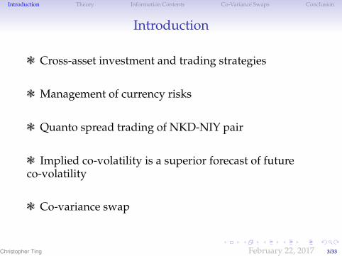
Introduction

c Cross-asset investment and trading strategies

c Management of currency risks

c Quanto spread trading of NKD-NIY pair

c Implied co-volatility is a superior forecast of futureco-volatility

c Co-variance swap



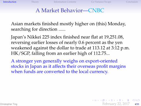
A Market Behavior—CNBC

Asian markets finished mostly higher on (this) Monday,searching for direction ......

Japan’s Nikkei 225 index finished near flat at 19,251.08,reversing earlier losses of nearly 0.6 percent as the yenweakened against the dollar to trade at 113.12 at 3:12 p.m.HK/SGP, falling from an earlier high of 112.75...

A stronger yen generally weighs on export-orientedstocks in Japan as it affects their overseas profit marginswhen funds are converted to the local currency.


http://www.cnbc.com/2017/02/19/asia-stocks-to-focus-on-trump-policies-dollar-strength-yen-and-earnings.html


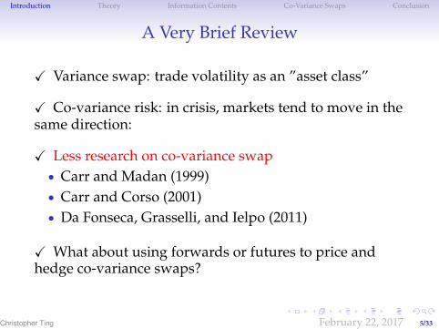
A Very Brief Review

X Variance swap: trade volatility as an ”asset class”

X Co-variance risk: in crisis, markets tend to move in thesame direction:

X Less research on co-variance swap• Carr and Madan (1999)• Carr and Corso (2001)• Da Fonseca, Grasselli, and Ielpo (2011)

X What about using forwards or futures to price andhedge co-variance swaps?



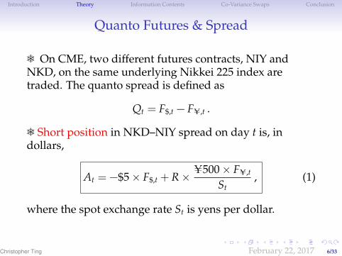
Quanto Futures & Spread

e On CME, two different futures contracts, NIY andNKD, on the same underlying Nikkei 225 index aretraded. The quanto spread is defined as

Qt = F$,t − FU,t .

e Short position in NKD–NIY spread on day t is, indollars,

At = −$5 × F$,t + R × U500 × FU,t

St, (1)

where the spot exchange rate St is yens per dollar.



Spread Trading Strategy



Proposition 1f Assuming that St remains constant, the quanto spreadposition is hedged against Nikkei index movements if and onlyif the ratio is given by

R =St

100.

f Proof: By substituting this R into equation 1, we obtain

At = −$5 × F$,t + $5 × FU,t

= $5 ×(− FU,t − Qt + FU,t

)= −$5 × Qt .

Suppose both NKD and NIY move up by x index points. The netnotional amount becomes Bt(x), and

Bt(x) = −$5 ×(F$,t + x

)+ R ×

U500 ×(FU,t + x

)St

= At − $5 x +St

100× U500 x

St= At − $5 x + $5 x = At .



Marked-to-Market Value

g The quanto spread seller is directly exposed tocurrency risk.

g If yen weakens, equivalently dollar strengthens, i.e.,Su > St, then the quanto seller may end up having soldthe NKD-NIY spread at a low value of Qt in comparisonto Qu + (1 − St/Su)FU,u, where Qu = F$,u − FU,u, u > t.

Au = $5 ×(−F$,u +

St

SuFU,u

)= $5 ×

(−FU,u − Qu +

St

SuFU,u

)= −$5 ×

(Qu +

(1 −

St

Su

)FU,u

).



P&L of a Quanto Spread Seller

c By unwinding the position at a later time u:

P&L(t, u) = 5 ×(

Qt − Qu −

(1 −

St

Su

)FU,u

)(2)

for every NKD contract.

c If the short quanto spread is held to maturity,

P&L(t, T) = 5Qt + 5(

1 −St

ST

)(NT−t − FU,t

)(3)

where NT is the value of Nikkei 225 Index at maturity T.



P&L in Different Scenarios for Q = 20



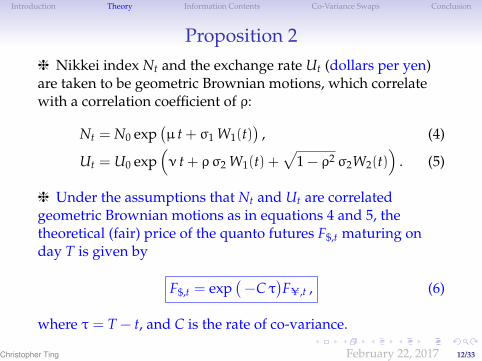
Proposition 2h Nikkei index Nt and the exchange rate Ut (dollars per yen)are taken to be geometric Brownian motions, which correlatewith a correlation coefficient of ρ:

Nt = N0 exp(µ t + σ1 W1(t)

), (4)

Ut = U0 exp(ν t + ρσ2 W1(t) +

√1 − ρ2 σ2W2(t)

). (5)

h Under the assumptions that Nt and Ut are correlatedgeometric Brownian motions as in equations 4 and 5, thetheoretical (fair) price of the quanto futures F$,t maturing onday T is given by

F$,t = exp(−C τ

)FU,t , (6)

where τ = T − t, and C is the rate of co-variance.



Geometric Brownian Motionö If an asset Vt follows the geometric Brownian motion

Vt = V0 exp(µ dt + σWt

),

then the log price Xt = ln(Vt) is an arithmetic Brownian motion

dXt = µ dt + σ dWt .

ö Treat Vt = exp(Xt) as a function of Xt. By Ito’s formula,

dVt = Vt dXt +12

Vt(dXt)2

= Vt µ dt +12

Vt σ2 dt + Vt σ dWt ,

leading to the stochastic differential equation,

dVt

Vt=

(µ+

12σ2)

dt + σ dWt .



Proof Setup÷ Risk-free rate r for money market account and yen moneymarket account Dt = exp(ut) of risk-free rate u for yen÷ Yen cash bond in dollars UtDt, and the Nikkei index indollars, UtNt.÷ Discounted money market account and Nikkei 225 Index indollars:

Yt = e−rtUtDt

Zt = e−rtUtNt

÷ Stochastic differential equations

dYt

Yt=(ν+ σ2

2/2 + u − r)dt + ρσ2 dW1(t) +

√1 − ρ2 σ2 dW2(t) ,

dZt

Zt=(µ+ ν+ σ2

1/2 + ρσ1σ2 + σ22/2 − r

)dt +

(σ1 + ρσ2)dW1(t)

+√

1 − ρ2 σ2 dW2(t) .



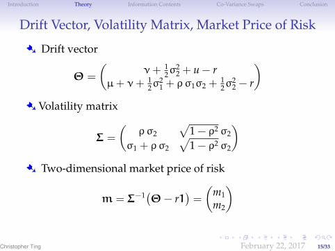
Drift Vector, Volatility Matrix, Market Price of Risk

÷ Drift vector

Θ =

(ν+ 1

2σ22 + u − r

µ+ ν+ 12σ

21 + ρσ1σ2 +

12σ

22 − r

)÷ Volatility matrix

Σ =

(ρσ2

√1 − ρ2 σ2

σ1 + ρσ2

√1 − ρ2 σ2

)÷ Two-dimensional market price of risk

m = Σ−1(Θ− r1)=

(m1m2

)



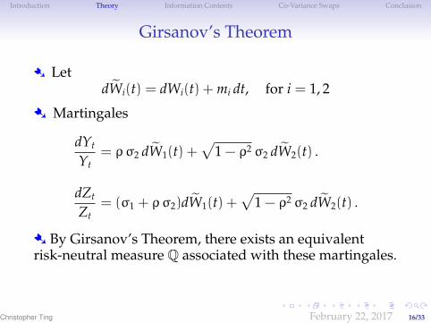
Girsanov’s Theorem

÷ LetdWi(t) = dWi(t) + mi dt, for i = 1, 2

÷ Martingales

dYt

Yt= ρσ2 dW1(t) +

√1 − ρ2 σ2 dW2(t) .

dZt

Zt= (σ1 + ρσ2)dW1(t) +

√1 − ρ2 σ2 dW2(t) .

÷ By Girsanov’s Theorem, there exists an equivalentrisk-neutral measure Q associated with these martingales.



Nikkei 225 Index Under Q÷ The stochastic differential equation for Nt is

dNt

Nt=(µ+ σ2

1/2)dt + σ1 dW1(t) .

Under Q with dW1(t) = dW1(t) + m1dt, this stochasticdifferential equation becomes

dNt

Nt= σ1 dW1(t) −

(µ+ σ2

1/2 + ρσ1σ2 − u)dt +

(µ+ σ2

1/2)dt

= σ1 dW1(t) +(u − ρσ1σ2

)dt .

÷ The solution is

Nt = N0 exp(σ1 W1(t) +

(u − ρσ1σ2 − σ

21/2)t)

.



Finally÷ At time t = 0, the theoretical forward price of Nikkei index isFU,0 = N0 exp

(uT). The solution is re-written as

NT = exp(−ρσ1σ2 T

)FU,T exp

(σ1W1(T) − σ2

1T/2)

.

÷ Let F$,0 be the forward price of the dollar-denominatedforward. The value v0 of this quanto forward at initiation iszero. Namely

v0 = EQ(NT − F$,0

)=(

exp(−ρσ1σ2 T)FU,0 − F$,0)= 0 .

÷ Consequently, under the risk-neutral measure Q,

F$,0 = exp(−ρσ1σ2 T

)FU,0 .

÷ Since C = ρσ1σ2, the pricing formula of the quanto forwardfor any t 6 T is therefore given by

F$,t = exp(−C (T − t)

)FU,t .



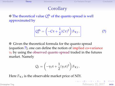
Corollary

i The theoretical value Qtht of the quanto spread is well

approximated by

Qtht =

(−Cτ+

12(Cτ)2

)FU,t . (7)

i Given the theoretical formula for the quanto spread(equation 7), one can define the notion of implied co-varianceγt by using the observed quanto spread traded in the futuresmarket. Namely

Qt =

(−γtτ+

12(γtτ)

2)

FU,t .

Here FU,t is the observable market price of NIY.



Implied Co-Variancej This equation is rewritten as

12(γtτ)

2 − γtτ−Qt

FU,t= 0 .

Solving this quadratic equation with respect to γtτ results in∗

γt =1 −

√1 + 2Qt/FU,t

τ. (8)

j Implied co-volatilityωt:

ωt := sign(γt)√∣∣γt

∣∣ . (9)

∗The other solution γtτ = 1 +√

1 + 2Qt/FU,t is not admissible because it isstrictly larger than 1, which is incompatible with the fact that the magnitudeof the co-variance between two returns on financial assets is usually less than1.



Co-Variance Swap

d Consider the returns of two assets and their respectivevolatilities σ1 and σ2. The covariance is C = ρσ1σ2

d Covariance swap is similar to variance swap:

Covariance realized over the tenor T − Risk-Neutral Covariance

d Key idea: use the quanto spread traded in the marketto back out a risk-neutral co-variance with the proposedmodel.



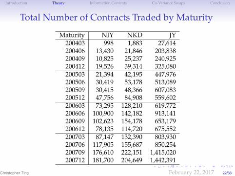
Total Number of Contracts Traded by Maturity

Maturity NIY NKD JY200403 998 1,883 27,614200406 13,430 21,846 203,838200409 10,825 25,237 240,925200412 19,526 39,314 325,080200503 21,394 42,195 447,976200506 30,419 53,178 513,089200509 30,415 48,366 607,083200512 47,756 84,908 559,602200603 73,295 128,210 619,772200606 100,900 142,182 913,141200609 102,623 154,178 653,179200612 78,135 114,720 675,552200703 87,147 132,390 803,930200706 117,905 155,687 850,254200709 176,610 222,151 1,415,020200712 181,700 204,649 1,442,391



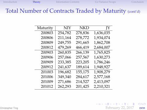
Total Number of Contracts Traded by Maturity (cont’d)

Maturity NIY NKD JY200803 254,782 278,836 1,636,035200806 211,164 278,772 1,934,074200809 249,755 291,665 1,862,708200812 479,269 466,419 2,684,007200903 260,835 266,139 1,765,825200906 257,066 257,567 1,630,273200909 233,385 223,205 1,786,246200912 241,637 189,614 1,948,927201003 196,682 155,175 1,908,279201006 349,340 284,617 2,577,168201009 271,686 214,527 2,413,097201012 262,293 201,425 2,210,321



Average Quanto Spreads

Maturity Days Mean Std Min Med Max200403 8 2.50 6.38 -8.33 3.75 10.00200406 56 1.28 4.42 -7.5 0.73 13.33200409 55 3.93 8.53 -6.36 2.69 57.50200412 63 2.54 2.31 -3.01 2.32 9.62200503 62 2.34 2.28 -2.97 2.18 8.57200506 67 2.42 1.84 -5.83 2.27 8.33200509 66 2.55 0.94 0.53 2.61 4.17200512 67 2.72 1.40 -0.44 2.62 7.71200603 66 5.99 3.72 -3.09 5.56 15.00200606 70 6.93 5.02 -2.48 5.07 19.69200609 68 4.66 4.99 -3.34 4.30 18.72200612 67 6.40 3.63 -0.62 6.13 16.16200703 67 6.83 3.54 -1.75 6.48 17.58200706 71 11.00 5.39 -1.77 12.00 22.66200709 74 8.17 5.31 0.88 7.28 20.00200712 71 24.97 11.03 0.47 27.42 48.92



Average Quanto Spreads (cont’d)

Maturity Days Mean Std Min Med Max200803 68 27.67 14.92 1.41 27.69 61.34200806 70 44.86 26.21 0.62 44.83 111.38200809 69 39.89 32.93 -0.22 39.25 117.85200812 72 69.33 40.74 0.53 64.93 182.94200903 67 82.28 55.39 -0.61 85.42 189.84200906 70 50.03 34.33 -0.21 46.71 120.16200909 71 47.00 22.20 0.23 50.43 87.92200912 67 29.63 25.30 0.26 18.15 96.76201003 69 37.26 23.22 0.15 36.98 81.82201006 71 27.46 19.64 -0.25 20.36 75.00201009 68 22.14 16.50 -0.13 18.66 57.65201012 69 23.79 13.85 0.27 19.20 54.32



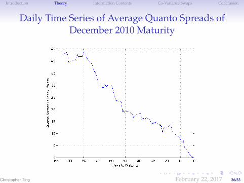
Daily Time Series of Average Quanto Spreads ofDecember 2010 Maturity



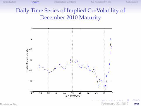
Daily Time Series of Implied Co-Volatility ofDecember 2010 Maturity



Rolling Historical Daily Co-Volatility



Realized Co-Volatility Regressed on ICVt and HCVt

σt(τ) = a + b1 ICVt(τ) + b2 HCVt(τ) + ut .

Days to Ave Num Adjustedmaturity (τ) τ Obs a t-stat b1 t-stat b2 t-stat R2

456 τ <50 46.7 69 -1.617 -0.89 0.264 1.83 0.603 4.00 0.6150506 τ <55 51.3 85 -0.213 -0.11 0.311 1.67 0.692 3.95 0.6299556 τ <60 57.5 95 0.298 0.14 0.580 2.50 0.445 3.25 0.5450606 τ <65 62.8 59 1.780 0.79 0.777 2.67 0.334 2.39 0.5858656 τ <70 65.9 62 0.485 0.17 0.698 1.83 0.343 2.06 0.5045706 τ <75 72.0 105 -0.800 -0.34 0.453 1.51 0.469 2.65 0.4244756 τ <80 78.0 61 -1.215 -0.47 0.626 2.23 0.283 1.79 0.3673806 τ <85 81.8 57 -1.956 -1.00 0.422 2.00 0.334 2.24 0.3849856 τ <90 86.5 93 -2.315 -1.01 0.455 1.97 0.216 1.23 0.3327906 τ <95 92.0 72 -1.528 -0.66 0.572 2.65 0.143 0.81 0.3351456 τ <95 69.3 758 -0.898 -0.82 0.516 3.99 0.359 3.65 0.4708



Co-Variance Swap

k On the maturity date T, the payoff to the swap buyer is

Payoff = C(t, T) − γt . (10)

Here the fixed leg is the risk-neutral implied co-varianceγt, which is determined by equation 8, and the floatingleg is the co-variance C(t, T) realized over the swap tenor.

C(t, T) =365

T − t − 1

T∑i=t+1

RN,iRU,i − RNRU ,



Average P&L of A Long Position in Co-Variance Swap



Conclusions

p A method to obtain implied co-variance from a pair offorwards

p Implied co-volatility is a superior forecast compared tohistorical forecast

p Shorting quanto spread on average does not gain overthe sample period 2005 through 2010

p Co-variance swaps are fair to both buyers and sellers

p A new method to price and hedge co-variance swaps.


Application of Stochastic Calculus to Price a Quanto Spread · Application of Stochastic Calculus...

Documents

Transcript of Application of Stochastic Calculus to Price a Quanto Spread · Application of Stochastic Calculus...