Appendix C Water Temperature Model and Analysis 2 Appendices... · C.1.2 Planning Objectives ......

Appendix C Water Temperature Model and Analysis

January 2010 – C-i

Contents Page

Abbreviations and Acronyms ................................................................................................... C-i

C.1 Introduction........................................................................................................................ C-1 C.1.1 Development of Temperature Model.........................................................................C-1 C.1.2 Planning Objectives ...................................................................................................C-2 C.1.3 Appendix Organization..............................................................................................C-3

C.2 Model Description.............................................................................................................. C-3 C.2.1 Temperature ...............................................................................................................C-4 C.2.2 Conservative Parameter/Tracer..................................................................................C-4 C.2.3 Model Representation of the Physical System...........................................................C-4 C.2.4 Model Representation of Reservoirs..........................................................................C-6 C.2.5 Model Representation of Streams............................................................................C-11 C.2.6 Hydrologic Boundary Conditions ............................................................................C-12 C.2.7 Temperature Boundary Conditions..........................................................................C-12 C.2.8 Meteorological Data.................................................................................................C-13

C.3 DMC Recirculation Analysis........................................................................................... C-22 C.3.1 Recirculation Model Representation........................................................................C-23 C.3.2 Model Results ..........................................................................................................C-24

C.4 References ......................................................................................................................... C-33

Tables Table C-1. Regression Relationships Among Three Observed Water Temperature

Datasets ................................................................................................................................C-24

Figures Figure C-1. Schematic of HEC-5 DMC Recirculation Model (shown in blue),

extending from New Melones Reservoir to Mossdale...........................................................C-5 Figure C-2. Schematic Representation of New and Old Melones Dams.....................................C-9 Figure C-3. End-of-Month Storage Volume in New Melones Reservoir as Computed

by HEC-5 and CalSim II......................................................................................................C-14

Delta-Mendota Canal Recirculation Feasibility Study Plan Formulation Report

C-ii – January 2010

Figure C-4. Time Series Plot of Water Temperature Boundary Condition for Stanislaus River above New Melones Reservoir .................................................................C-15

Figure C-5. Time Series Plot of Water Temperature Boundary Condition for San Joaquin River above Stanislaus River..................................................................................C-16

Figure C-6. California Data Exchange Center-Observed Water Temperatures at Vernalis and Model Water Temperature Boundary Condition Applied at San Joaquin River above Stanislaus River..................................................................................C-17

Figure C-7. Computed Water Temperatures at Goodwin Dam Using 4-Year Average Meteorology and Individual Year Meteorology (regression between two results and R2 value shown)............................................................................................................C-19

Figure C-8. Computed Water Temperatures at Oakdale Recreation Using 4-Year Average Meteorology and Individual Year Meteorology (regression between two results and R2 value shown) ................................................................................................C-20

Figure C-9. Computed Water Temperatures at Vernalis Using 4-Year Average Meteorology and Individual Year Meteorology (regression between two results and R2 value shown)............................................................................................................C-21

Figure C-10. Observed Water Temperatures at the Delta Pumps, Mossdale, and Vernalis for 1999 through 2005...........................................................................................C-25

Figure C-11. Observed Water Temperatures at the Delta Pumps, Mossdale, and Vernalis for 2000 .................................................................................................................C-26

Figure C-12. Computed No-Action Alternative and Alternative D Water Temperatures and Flows below Goodwin Dam for 1991–1994..........................................C-27

Figure C-13. Computed No-Action Alternative and Alternative D Water Temperatures at Oakdale Recreation and Flows below Goodwin Dam for 1991–1994......................................................................................................................................C-28

Figure C-14. Computed No-Action Alternative and Alternative D Water Temperatures on the Stanislaus River above the Confluence and Flows at Ripon for 1991–1994......................................................................................................................C-29

Figure C-15. Computed No-Action Alternative and Alternative D Water Temperatures and Flows at Vernalis for 1991–1994...........................................................C-31

Figure C-16. Computed No-Action Alternative and Alternative D Flows at Ripon and Vernalis .........................................................................................................................C-32

January 2010 – C-iii

Abbreviations and Acronyms CalSim II California Simulation Model II CIMIS California Irrigation Management Information

System CVP Central Valley Project Delta Sacramento-San Joaquin River Delta DMC Delta-Mendota Canal DSS Data Storage System DSM2 Delta Simulation Model II DWR California Department of Water Resources NWS National Weather System Reclamation Bureau of Reclamation SJR San Joaquin River Study DMC Recirculation Project Feasibility Study WES Waterways Experiment Station

January 2010 – C-1


C.1 Introduction

The U.S. Department of the Interior, Bureau of Reclamation (Reclamation) is evaluating the feasibility of using recirculation strategies to improve water quality and flows in the lower San Joaquin River (SJR). Specifically, Reclamation is evaluating the feasibility of the Delta-Mendota Canal (DMC) Recirculation Project, which involves recirculating water from the Sacramento-San Joaquin River Delta (Delta) through the Central Valley Project (CVP) pumping and conveyance facilities to the SJR, upstream from Vernalis, the point at which SJR enters the Delta.

This Plan Formulation Report, which is a component of the overall DMC Recirculation Project Feasibility Study (Study), describes the planning process used to develop and evaluate alternative plans for the Study. The Study will culminate in an Environmental Impact Statement/Environmental Impact Report and a Feasibility Report, including a Record of Decision and a Notice of Determination. Reclamation is the federal lead agency for National Environmental Policy Act compliance and the California Department of Water Resources is the state lead agency for California Environmental Quality Act compliance.

The purpose of the Study is to identify and evaluate the feasibility of implementing DMC recirculation as a means of accomplishing the objectives defined in the authorizing language. The Study, which is identified in the authorizing legislation as part of Reclamation’s overall Program to Meet Standards, will determine whether Reclamation can, through the use of excess capacity in export pumping and conveyance facilities, provide greater flexibility in meeting the existing water quality standards and flow objectives for which the CVP has responsibility, reduce the demand on water from New Melones Reservoir (for use to improve water quality and flow), and assist the Secretary of the Interior in meeting any obligation to CVP water contractors using New Melones Reservoir.

C.1.1 Development of Temperature Model

In the late 1990s, a group of stakeholders on the Stanislaus River initiated a cooperative effort to develop a water temperature model for the Stanislaus River having recognized the need to analyze the relationship between operational


C-2 – January 2010

alternatives, water temperature regimes, and fish mortality in the Stanislaus River. These stakeholders included Reclamation, U. S. Fish and Wildlife Service, California Department of Fish & Game, Oakdale Irrigation District, South San Joaquin Irrigation District, and Stockton East Water District. In December 1999, these partners garnered the necessary funding and through a cost-sharing arrangement retained AD Consultants in association with its subconsultant Research Management Associates to develop the model and perform a preliminary analysis of operational alternatives. In addition, the cost-sharing partners launched an extensive program for water temperature and meteorological data collection throughout the Stanislaus River Basin, in support of the modeling effort.

In 2003 the project was extended to include the lower SJR through a CALFED grant (ERP-02-P28) to Tri-Dam (recipient). A principal priority of this CALFED-sponsored project was to develop a model capable of evaluating a wide range of alternatives for flow and water temperature management in the Stanislaus River and lower SJR.

In December 2004, CALFED decided to extend the Stanislaus–lower San Joaquin River Water Temperature Model to include the Tuolumne and Merced rivers, and the main-stem SJR from Stevenson to Mossdale (to be known as the San Joaquin River (SJR) Basin-Wide Water Temperature Model). The work was to be performed in two stages: (1) through an amendment to the existing recipient agreement with Tri-Dam (ERP-02-P28) and (2) through a 2-year Directed Action, thereafter.

Under the amended scope, the recipient developed a beta version of the model. This work was presented to CALFED and approved by a CALFED-sponsored peer review (separate from the peer review panel assessing thermal criteria). The Directed Action allowed further refinement of the model and, using the model, investigation of various mechanisms for water temperature improvements through operational and/or structural measures at existing facilities in all three SJR tributaries of the.

C.1.2 Planning Objectives

The primary objective of this study is to evaluate the potential effects to temperatures in the Stanislaus River due to implementation of the DMC Recirculation Project. Changes in temperature as a result of recirculation may result in effects in meeting water quality objectives (evaluated in Appendix F) and/or effects on fisheries resources in the affected areas (evaluated in Appendix H).



To achieve the planning objective, the project team implemented an abbreviated version of the previously calibrated HEC-5Q model of the Stanislaus–lower SJR system. The project team analyzed the results and selected the flow alternative with the greatest temperature consequences (Alternative D) for presentation in this appendix.

C.1.3 Appendix Organization

This appendix is designed to provide a description of the overall work and the necessary background needed for interpreting model results. Evaluation of the potential thermal impacts on the aquatic environment of the various alternative recirculation scenarios is not included. The appendix is divided into four sections: Section C.1 provides an overview of the project and its objectives. Section C.2 describes the HEC-5Q model and its adaptation to the Stanislaus–lower SJR system. Section C.3 presents the recirculation model and results. Section C.4 contains references cited in this appendix.

C.2 Model Description

The water quality simulation module (HEC-5Q) was developed to assess temperature and a conservative water quality constituent in basin-scale planning and management decision making. The application of HEC-5Q to the Stanislaus River and lower SJR computes the vertical or longitudinal distribution of temperature in the reservoirs and longitudinal temperature distributions in stream reaches based on daily average flows.

HEC-5Q can be used to evaluate options for coordinating reservoir releases among projects to examine the effects on flow and water quality at specified locations in the system. Example applications of the flow simulation model include examination of reservoir capacities for flood control, hydropower, and reservoir release requirements to meet water supply and irrigation demands. The model can be applied to a wide array of applications including evaluation of in-stream temperatures and several water quality constituent concentrations at critical locations in the system, examination of the potential effects of changing reservoir operations, and/or water use patterns on temperature or water quality constituent concentrations. Further, reservoir selective withdrawal operations (either existing or proposed facilities) can be simulated using HEC-5Q to determine necessary operations to meet water quality objectives downstream.

The HEC-5Q model used in the DMC recirculation analysis utilized only temperature and the conservative tracer (for mass continuity checking). A brief description of the processes affecting these two parameters is provided below.



Refer to the HEC-5Q users manual (HEC 2001) for a more complete description of the water quality relationships included in model.

C.2.1 Temperature

The external heat sources and sinks that were considered in HEC-5Q were assumed to occur at the air-water and the sediment-water interfaces. Equilibrium temperature and coefficient of surface heat exchange concepts were used to evaluate the net rate of heat transfer. Equilibrium temperature is defined as the water temperature at which the net rate of heat exchange between the water surface and the overlying atmosphere is zero. The coefficient of surface heat exchange (Joules/m2·oK·sec) is the rate at which the heat transfer process progresses. All heat transfer mechanisms, except short-wave solar radiation, were applied at the water surface. Short-wave radiation penetrates the water surface and may affect water temperatures below the air-water interface. The depth of penetration is a function of adsorption and scattering properties of the water as affected by particulate material (i.e., phytoplankton and suspended solids). The heat exchange with the bottom is a function of conductance and the heat capacity of the bottom sediment.

C.2.2 Conservative Parameter/Tracer

The conservative parameter is unaffected by decay, settling, uptake, or other processes and, thus, acts as a tracer – passively transported by advection and diffusion. This parameter was used to check mass continuity by setting the concentration of the tracer in all inflows to a constant value and then checking to ensure simulation results reproduced the specified concentration.

C.2.3 Model Representation of the Physical System

The DMC recirculation temperature model incorporates the Stanislaus River system, including New Melones, Tulloch, and Goodwin reservoirs, and the SJR from the Stanislaus River to Mossdale Bridge (see Figure C-1). This model is a subset of the original CALFED Stanislaus-Lower SJR model.

Rivers and reservoirs within the DMC recirculation model were represented as a network of discrete sections (reaches and/or layers, respectively) for application of HEC-5 for flow simulation and HEC-5Q for temperature simulation. Within this network, control points were designated to represent reservoirs and selected stream locations where flow, elevations, and volumes were computed. In HEC-5, flows and other hydraulic information are computed at each control point (HEC 1998). Within HEC-5Q, stream reaches and reservoirs were partitioned into computational elements to compute spatial variations in water temperature



Stanislaus River

New Melones Reservoir

Tulloch Reservoir

Goodwin Reservoir

San Joaquin

River

Ripon

Mossdale Bridge

Oakdale Rec. Area

Figure C-1. Schematic of HEC-5 DMC Recirculation Model (shown in blue), extending from New Melones Reservoir to Mossdale



between control points. Within each element, uniform temperature was assumed; therefore, the element size determines the spatial resolution. The model representation of reservoirs and streams is summarized in Sections C.2.2 and C.2.3.

C.2.4 Model Representation of Reservoirs

Within HEC-5Q, reservoirs can be represented as vertically or longitudinally segmented water bodies. Longitudinally segmented reservoirs can be vertically layered within the segments. Typically, the vertically segmented representation is applied to reservoirs that are prone to seasonal stratification, while longitudinally segmented representations are applied to impounded waters that retain riverine characteristics (e.g., a short residence time, intermittent/weak, stratification).

For water quality simulations, New Melones and Tulloch reservoirs were geometrically discretized and represented as vertically segmented water bodies with segments approximately 2 feet thick.

Goodwin Reservoir was represented as longitudinally segmented with nine segments. Each segment has five layers, with each layer representing 1/5 of the cross-sectional area (in the lateral by vertical plane).

Model time steps were 6 hours.

A description of the different types of reservoir representation follows.

Vertically Segmented Reservoirs (one-dimensional)

Vertically stratified reservoirs are represented conceptually by a series of one-dimensional horizontal slices or layered volume elements, each characterized by a surface area, thickness, and volume. The aggregate assemblage of layered volume elements is a geometrically discretized representation of the prototype reservoir. The geometric characteristics of each horizontal slice are defined as a function of the reservoir’s area-capacity curve. Within each horizontal layer (or ‘element’) of a vertically segmented reservoir, the water is assumed to be fully mixed with all isopleths parallel to the water surface both laterally and longitudinally. External inflows and withdrawals occur as sources or sinks within each element and are instantaneously dispersed and homogeneously mixed throughout the layer from the headwaters of the impoundment to the dam. Consequently, simulation results are most representative of conditions in the main reservoir body and may not accurately describe flow or quality characteristics in shallow regions or near reservoir banks. It is not possible to model longitudinal variations in water quality constituents using the vertically segmented configuration.



The allocation of the inflow to individual elements is based on the relative densities of the inflow and the reservoir elements. Flow entrainment is considered as the inflowing water seeks a depth or level of similar density.

Vertical advection is one of two transport mechanisms used in HEC-5Q to simulate transport of water quality constituents between elements in a vertically segmented reservoir. Vertical advection is defined as the interelement flow between adjacent elements. An additional transport mechanism used to distribute water quality constituents between elements is effective diffusion, representing the combined effects of molecular and turbulent diffusion, and convective mixing, the physical movement of water due to density instability. Wind- and flow-induced turbulent diffusion and convective mixing are the dominant components of effective diffusion in the epilimnion of most reservoirs.

The outflow component of the model incorporates a selective withdrawal technique for withdrawal through multiple dam outlets or other submerged orifices, or for flow over a weir. The relationships developed for the ‘Waterways Experiment Station (WES) Withdrawal Allocation Method’ (Bohan and Grace 1973) describe the vertical limits of the withdrawal zone and the vertical velocity distribution throughout the water column.

For the DMC Recirculation model application, the existing conditions incorporated into HEC-5Q include:

(1) New Melones power intake (from top of intake pipe at elevation 775 feet) is always utilized for water-surface elevations greater than 786.5 feet. The low-level outlet (two pipes) operates at lake elevations less than 786.5 feet. New Melones Spillway has never been used although it would be if releases greater than 7,700 cubic feet per second occurred.

(2) Tulloch low level (power intake) is always used except for flows greater than 2,060 cubic feet per second. Excess flows are passed through the gated spillway.

Longitudinally Segmented Reservoirs (two-dimensional)

Longitudinally segmented reservoirs represent reservoirs two-dimensionally in the longitudinal and vertical directions. They are represented conceptually as a linear network of a specified number of segments or volume elements. The length of a segment, coupled with an associated stage-width relationship, characterizes the geometry of each reservoir segment. Surface areas, volumes, and cross-sectional areas are computed from the stage-width relationship.



Additionally, longitudinally segmented reservoirs can be subdivided into vertical elements, with each element assumed fully mixed in the vertical and lateral directions. Branching of reservoirs is allowed. For longitudinally segmented reservoirs with layers, all segments contain the same number of layers and each layer extends the full length of the segment. Layers are assigned equal fractions of the cross-sectional area (in the lateral by vertical plane) of the segment. Therefore, the depth of each layer varies with reservoir stage according to the width versus elevation relationship for each segment. The model performs a backwater computation to define the water-surface profile as a function of the hydraulic gradient based on flow and Manning’s equation.

A uniform vertical flow distribution is specified at the upstream end of each reservoir. Velocity profiles within the body of the reservoir may be calculated as flow over a submerged weir or they may be specified as a function of a density profile. Linear interpolation is performed for reservoir segments that lie between these specifically defined flow fields

External flows, such as withdrawals and tributary inflows, occur as sinks or sources within the segment. Inflows to the upstream ends of reservoir branches are allocated equally to individual layers in the segment. Other minor side inflows to the reservoir are distributed in proportion to the local reservoir flow distribution as an expediency to maintain mass continuity. If the inflow is potentially large (which is not the case for Goodwin Reservoir), a branched reservoir would be required with a uniform upstream velocity profile. External flows may be allocated along the length of the reservoir to represent dispersed nonpoint source inflows such as agricultural drainage and groundwater accretions.

Vertical variations in constituent concentrations can be computed for the layered and longitudinally segmented reservoir model. Mass transport between vertical layers is represented by net flow determined by mass balance and by diffusion.

Vertical flow distributions at dams are based on weir or orifice withdrawal. The velocity distribution within the water column is calculated as a function of the water density and depth using the WES weir withdrawal or orifice withdrawal allocation method

For the DMC Recirculation model application, the existing conditions incorporated into HEC-5Q include Goodwin Dam, which currently has no low-level outlet. The seasonally warmer surface waters are, thus, preferentially released to the river (over the spillway, elevation 359 feet), and deeper, cooler water is diverted to the two water districts.



New Melones Reservoir

New Melones Reservoir is a large impoundment that is subject to strong seasonal stratification. Of special interest are the representation of New Melones Reservoir and, in particular, the impacts of the old dam on the flow and thermal regime of the reservoir and the reservoir release temperatures.

A schematic representation of the New and Old Melones dams is shown on Figure C-2. Flow allocation at different reservoir storage volumes includes:

Flow allocation when using the existing New Melones Dam primary (power) outlet

Flow allocation when in transition from primary outlet operations to the low-level outlet with the water surface above the old dam spillway invert

Flow allocation below old dam spillway invert.

As the reservoir fills, the flow allocation logic applies in reverse. Each of these allocations is discussed in greater detail below.

Spillway El. 1088

Crest El. 1135

Min. Power Pool El. 785Intake El. 760

Crest El. 735Spillway El. 723

El. 543

El. 610

Transition Zone: 3-4 feet

New DamOld Dam

Not to Scale

Vol. 2,400 AF

Figure C-2. Schematic Representation of New and Old Melones Dams



Flow Allocation Using New Melones Dam Primary Outlet (water-surface elevation greater than 785 feet) The primary intake for New Melones Dam is at elevation 760 feet (invert elevation) and the top of the intake structure is approximately 775 feet. The minimum pool elevation for hydropower production is approximately 785 feet. The model code has been modified to limit the lower extent of the withdrawal envelope (calculated with the WES method) to the top of the old dam for elevations above 785 feet (785 feet to full pool, approximately 1,088 feet). Below 785 feet the low-level outlet is used due to operational constraints.

Flow Allocation When in Transition from Primary Outlet Operations to Old Dam Spillway Invert (water-surface elevation 785 to 723 feet) When water levels in New Melones Reservoir drop below 785 feet, reservoir withdrawals are no longer made from the primary intake, but instead are drawn from the low-level outlet (elevation 543 feet). For water levels from 785 to 728 feet (5 feet above old dam spillway invert), all water is assumed to pass over the crest and/or over the spillway of the old dam. These flows are represented with an orifice equation where the area and elevation (relative to the old dam spillway elevation) is a function of the approach velocity. The outlet works release temperature is computed directly using the WES withdrawal method. As flow increases, the dimensions of the orifice (area and centerline elevation) are increased to maintain an approach velocity of 0.1 foot per second. This method was used because the model required some constraints during the transition between the old dam spillway and power outlet for numerical stability. These constraints impact the results for a few days during the entire simulation.

When the reservoir level drops to within 5 feet of the old dam spillway crest, the model transitions from flow passing solely over the old dam to a combined passage of both over the old dam spillway and through the low-level outlet in the old dam. The total flow transitions linearly from all flow passing over the top of the dam at 5 feet above the spillway invert to all of the flow passing through the old dam low-level intake when the reservoir level reaches the spill invert. This approach assumes that the old dam power outlet is open prior to surfacing of the old dam spillway.

The interdam region (volume) is not explicitly modeled because the quantity of water between the dams is small when the reservoir drops to the crest elevation of the old dam (approximately 2,400 acre-feet). If the reservoir is stratified during the transition period, warm waters flow over the top of the old dam and cooler waters flow through the low-level intake. The New Melones Reservoir release temperature is calculated using a mass balance: water that passes over the dam and water that passes through the low-level intake are assumed mixed completely and instantaneously in proportion to their total quantity.



Flow Allocation below Old Dam Spillway Invert (water-surface elevation less than 723 feet) Once below the old dam spillway invert, all flows are passed through the low-level outlet and assigned a withdrawal envelope according to the WES withdrawal approach and the physical characteristics of the old dam power intake.

C.2.5 Model Representation of Streams

In HEC-5Q, river or stream reaches are represented conceptually as a linear network of segments or volume elements. The length, width, cross-sectional area, and a flow versus depth relationship characterize each element. Cross sections are defined at all control points and at intermediate locations where data are available. The flow versus depth relation is developed external to HEC-5Q using available cross-sectional data and appropriate hydraulic computations. Linear interpolation between input cross-sectional locations is used to define the hydraulic data for each element.

For the Stanislaus River, two river reaches are modeled: between New Melones Dam and Tulloch Reservoir, and from Goodwin Dam to the confluence with the SJR. Downstream of New Melones, U.S. Army Corp of Engineers cross sections, field reconnaissance, and aerial photographs were used to define the geometry of the stream reaches.

The SJR reach is from Stanislaus River confluence to Mossdale Bridge.

Flow rates are calculated at stream control points by HEC-5 using one of several available hydrologic routing methods. For this project, all flows were routed using specified routing that explicitly defines travel time between control points. Within HEC-5, incremental local flows (i.e., flow between adjacent control points such as inflows or withdrawals may include any point or nonpoint flow) are assumed to enter at the control point. Within HEC-5Q, incremental local flow for a particular reach may be divided into components and placed at different locations within the stream reach (i.e., that portion of the stream bounded by the two control points). The diversions (demands) are allocated to individual control points within the river reaches or reservoirs. Distributed flows such as groundwater accretions and nonspecific agricultural return flows are defined on a rate per mile basis. A flow balance is used to determine the flow rate at element boundaries.

For simulation of water quality (e.g., temperature), the tributary locations and associated water quality are specified (see next section). To allocate components of the diversion flow balance, HEC-5Q performs a calculation using any specified withdrawals, inflows, or return flows, and distributes the



balance uniformly along the stream reach. Once interelement flows are established, the water depth, surface width, and cross sectional area are computed at each element boundary, assuming normal flow and downstream control (i.e., backwater). This study had no return flows other than groundwater. Stream elements were approximately 1 mile long. Consistent with the reservoir representation, model time steps were 6 hours in length.

C.2.6 Hydrologic Boundary Conditions

HEC-5Q requires that flow rates and water quality be defined for all inflows. Only four inflows are included in the model: New Melones and Tulloch reservoir inflows, Ripon accretions, and SJR inflow. For recirculation simulations (Section C.3), recirculation flows are added to the SJR inflow. All four inflows were defined explicitly by monthly average California Simulation Model II (CalSim II) values. An exception to the monthly defined flows occurs in April and May when pulse flows occur. During these 2 months, flows change mid-month. Reservoirs were operated to meet submonthly CalSim II flows at Goodwin Dam.

CalSim II and HEC-5 compute slightly different mass balance, as shown in the Figure C-3 plot of New Melones end-of-month storage volumes computed by the two models. The reason for the difference is not known. Perhaps it is due to different rounding methods. In any case, the volume difference is trivial and insignificant for temperature computations.

C.2.7 Temperature Boundary Conditions

Inflow temperatures for New Melones and the SJR in the DMC Recirculation model were computed at 6-hour intervals using the original Stanislaus–Lower SJR model (AD Consultants et al. 2007). Inflow temperatures to New Melones were computed as a flow (historical)-weighted thermal balance of inflows from the Stanislaus and Collierville powerhouses and the Middle and South Forks of the Stanislaus River. The SJR temperatures above the Stanislaus confluence were computed based on the historical flows and operation of the Merced, Tuolumne, and San Joaquin rivers. These computed temperature boundary conditions, shown on Figures C-4 and C-5, were used for all alternative plans. For Tulloch and Ripon accretions, temperatures were computed based on relationships developed from available ambient temperature data. Alternative simulations had no variation in inflow temperatures.

For the original Stanislaus–Lower SJR model, temperature relationships were developed from observed hourly California Data Exchange Center and project data for the period of 1999 through 2005. These data were analyzed and a composite relationship was developed that considered meteorology (equilibrium



temperature), flow rate, and a seasonal temperature distribution. The seasonal temperatures were defined to represent high-flow conditions (e.g., elevated flows due to snowmelt). High flows had a seasonal bias and Lower flows had an equilibrium temperature bias. Flow rate also influenced the diurnal variation with a large range of inflow temperatures at lower flows and shallower water depths. The temperatures of stream accretions were assumed equal to the ambient stream temperature. Very limited small stream/return flow temperature data suggest that this approximation is reasonable; however, the current data collection effort may provide sufficient data to further refine this approximation.

On Figure C-6, California Data Exchange Center-observed water temperatures at Vernalis are plotted with SJR model boundary condition temperatures. The boundary condition temperatures are slightly higher because they do not include the cooling effects of the Stanislaus River. At times when the differences between the two time series are greatest, the Stanislaus River flow is higher.

C.2.8 Meteorological Data

For temperature simulation using HEC-5Q, specification of water-surface heat exchange data requires designation of meteorological zones within the study area. Each control point within the system or subsystem used in temperature or water quality simulation must be associated with a defined meteorological zone. Meteorological zones represent hourly data from the Modesto California Irrigation Management Information System (CIMIS) station for the period of 1989–2005.

Meteorological data for the 1980–1988 period were developed by extrapolation of the CIMIS data based on daily National Weather Service (NWS) maximum and minimum air temperature data for Modesto. The relationship between the maximum and minimum air temperatures of the CIMIS and NWS data was developed by comparing data for each day that air temperatures were available (1989–2002). For each day when CIMIS data were unavailable, the NWS temperature extremes were adjusted using the relationship described above and then the hourly CIMIS data that best replicated the NWS extreme were selected for use in the model. The CIMIS records considered were limited to within 2 days before or after the calendar day; thus, up to 5 days from each of the 17 years (1989–2005) of CIMIS data (a maximum of 85 days) were considered.



0

500000

1000000

1500000

2000000

2500000

3000000

1-Jan-80 1-Jan-84 1-Jan-88 1-Jan-92 1-Jan-96 1-Jan-00 1-Jan-04

Ne

w M

elo

nes

Sto

rag

e V

olu

me

, Ac-

ftHEC-5 Result

CalSim Result

Figure C-3. End-of-Month Storage Volume in New Melones Reservoir as Computed by HEC-5 and CalSim II



40

45

50

55

60

65

70

75

80

85

90

Jan-86 Jan-87 Jan-88 Jan-89 Jan-90 Jan-91 Jan-92 Jan-93

Wa

ter T

em

pe

ratu

re, d

eg

F

Figure C-4. Time Series Plot of Water Temperature Boundary Condition for Stanislaus River above New Melones Reservoir



40

45

50

55

60

65

70

75

80

85

90


Wat

er T

emp

erat

ure,

deg

F

Figure C-5. Time Series Plot of Water Temperature Boundary Condition for San Joaquin River above Stanislaus River



40

45

50

55

60

65

70

75

80

85

90

Jan-99 Jan-00 Jan-01 Jan-02 Jan-03 Jan-04

Wat

er

Te

mp

era

ture

, de

g F

Vernalis-CDEC

Model BC at San Joaquin River

Figure C-6. California Data Exchange Center-Observed Water Temperatures at Vernalis and Model Water Temperature Boundary Condition Applied at San Joaquin River above Stanislaus River



Hourly air temperature, wind speed, relative humidity, and cloud cover for each day are used to compute the average equilibrium temperature, surface heat exchange rate, solar radiation flux, and wind speed at 6-hour intervals for input to HEC-5Q. Solar radiation and wind speed are used in the reservoir simulation to attenuate solar energy below the water surface and to compute wind-induced turbulent mixing parameters.

The 6-hour time interval is used to capture the diurnal variation. An hourly time step results in essentially the same maximum and daily average as a 1-hour simulation. The HEC-5Q GUI that is often used to demonstrate model results becomes cumbersome with 1-hour output (6 times larger files and even greater time delay due to the file size).

Three meteorological zones were used in the Stanislaus River model. Heat exchange coefficients for each zone were computed to reflect typical environmental conditions. For sheltered stream sections, wind speed was reduced and shading was assumed to reflect riparian canopy conditions. Reduced wind speed decreases the evaporative heat loss and results in higher equilibrium temperatures and lower heat exchange rates. Shading reduces solar radiation resulting in lower equilibrium temperatures and lower heat exchange rates. No riparian shading was assumed for reservoirs and for the lower SJR. For New Melones and Tulloch reservoirs the wind speed was increased to reflect open-water conditions.

More information about the methods employed in processing and incorporating meteorological data in the model is available in the Stanislaus–Lower San Joaquin River Water Temperature Modeling and Analysis final report (AD Consultants et al. 2006).

For the current study, 4 years of meteorology were selected from this period and averaged together. The years were selected by URS to represent typical conditions for four water year types: 1992, a typical “critical” year; 1993, a typical “wet” year; 2002 a typical “dry” year; and 2003 a typical “below normal” year. No “above normal” water year occurred during the simulation period (1980–2003).

The reason for averaging the meteorology for the 4 years was to eliminate variations for different hydrologic year types so they would not mask other differences of interest. To assure that this approach was reasonable, simulations were run for 1986–1992 with the 4-year averaged meteorology and with the actual meteorology for the individual years. Time series plots are provided for comparison at Goodwin (Figure C-7), Oakdale Recreation (Figure C-8), and Vernalis (Figure C-9). Regressions between the two results were computed and are noted on each plot. At each location, regressions were nearly one to one



40

45

50

55

60

65

70

75

80

85

90


Wa

ter

Tem

pe

ratu

re,

de

g F

Goodwin 4-year average

Goodwin

Figure C-7. Computed Water Temperatures at Goodwin Dam Using 4-Year Average Meteorology and Individual Year Meteorology (regression between two results and R2 value shown)



40

45

50

55

60

65

70

75

80

85

90


Wa

ter

Tem

pe

ratu

re,

de

g F

Oakdale Rec 4-year average

Oakdale Rec

Figure C-8. Computed Water Temperatures at Oakdale Recreation Using 4-Year Average Meteorology and Individual Year Meteorology (regression between two results and R2 value shown)



40

45

50

55

60

65

70

75

80

85

90


Wa

ter

Tem

pe

ratu

re,

de

g F

Vernalis 4-year average

Vernalis

Figure C-9. Computed Water Temperatures at Vernalis Using 4-Year Average Meteorology and Individual Year Meteorology (regression between two results and R2 value shown)



with R2 values of 0.95 or greater. This close correlation between the results indicates that the use of averaged temperatures does not strongly impact the results and is, thus, a reasonable approach.

Figure C-7 shows a thermal regime at Goodwin Dam that is strongly influenced by the New Melones Dam operation that is described in Section C2.2.3. The increase in yearly maximum temperatures during the plotted period is the result of decreasing reservoir volume and resulting access to the metalimnion. The sharp drop in temperature in mid 1992 results from the transition between power generation and bypass to the low-level outlet. The subsequent increase in fall 1992 is due to warmer water flowing over the old dam as the New Melones elevation continues to fall. This temperature response is seen in the alternative analysis results and small differences in reservoir volume impact the timing of the transition between outlets.

C.3 DMC Recirculation Analysis

The model was used to evaluate the DMC Recirculation Project, which involves recirculating Delta water to the SJR, upstream of the confluence with the Stanislaus River, via the CVP pumping and conveyance facilities to improve water quality and flows in the lower SJR.

In this appendix, two scenarios are analyzed: a No-Action Alternative scenario (no action under future level of development) and Alternative D (an alternative plan using future level of development). Several alternative plans, which vary in timing and volume of recirculation flow, were simulated. The simulation results for each alternative plan were delivered to study partners as Data Storage System (DSS) output and in tabular form. The DSS output included reservoir elevation and volume and stream flow and temperatures at 6-hour intervals for selected locations. The DSS output is intended as a platform for visually comparing alternative plans. The tabular output provided 6-hour temperatures at all stream locations (96 points). Each stream location is identified by river mile from upstream to downstream. Key river mile locations include:

Mile 142.4 – New Melones Dam

Mile 134.9 – Tulloch Dam

Mile 131.0 – Goodwin Dam

Mile 127.3 – Stanislaus River at Knights Ferry

Mile 119.0 – Stanislaus River at Orange Blossom Bridge



Mile 106.4 – Stanislaus River at Riverbank Bridge

Mile 87.8 – Stanislaus River at Ripon

Mile 72.5 – Stanislaus River at the San Joaquin confluence

Mile 69.3 – San Joaquin River at Vernalis

Mile 56.7 – San Joaquin River at Mossdale

Alternative D was chosen for presentation because it resulted in the greatest changes to temperature. Detailed output for all alternative plans evaluated is discussed further in the water quality analysis (Appendix F) and the aquatic biological resources analysis (Appendix H).

C.3.1 Recirculation Model Representation

For the recirculation scenarios, such as Alternative D, water is recirculated from the Delta, through the Newman Wasteway and/or Westley Waterway, back to the SJR, allowing reductions in New Melones Reservoir releases. Both the recirculation flows and the modified New Melones releases were computed using CalSim II (Appendix A). The recirculation is represented in the model as an inflow to the SJR upstream of the confluence (the upstream model boundary on the SJR). The DMC, wasteways, and the SJR above the Stanislaus River are not represented in the model.

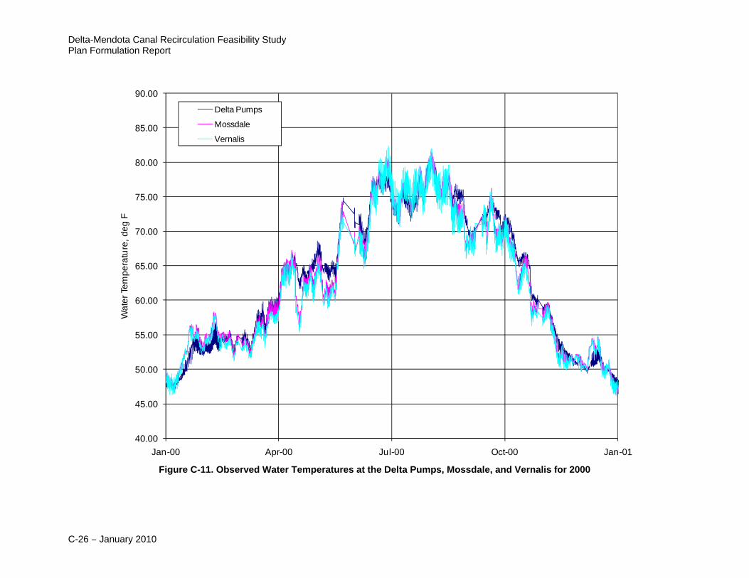
The same temperature boundary applied to the SJR flows (see Figure C-5) is used for the recirculation flows. Any minor temperature impacts of the recirculation flow are ignored because observed temperatures at the DMC, Mossdale, and Vernalis are all similar, but with greater diurnal variation in the nontidal river. This scenario is illustrated on Figure C-10, showing water temperatures for the three locations for 1999 through 2005, with an expanded view of 2000 on Figure C-11. Regressions among the three datasets are summarized in Table C-1. Relationships among the datasets are all nearly one to one with R2 values of 0.95 or greater. Differences among the three datasets are within the range of thermal impacts from hydrologic variability. The assumption is that because the Delta and the SJR above the confluence are near equilibrium, temperatures in the SJR above the confluence will not vary significantly as the proportion of recirculation flow changes.

Because of the model representation and assumptions, the model cannot quantify impacts of recirculation on Delta pump water temperature nor SJR temperatures above the Stanislaus River confluence.



Table C-1. Regression Relationships Among Three Observed Water Temperature Datasets

X Y Y/X R2

Delta pumps Vernalis 0.9914 0.9507

Mossdale Vernalis 0.9896 0.9883

Mossdale Delta pumps 0.9974 0.9651

C.3.2 Model Results

Comparisons have been made between the No-Action Alternative and Alternative D model results for the 1991 through 1994 period, at locations throughout the system. Shown on Figure C-12 are time series plots of computed water temperature and outflow from Goodwin Dam for the No-Action Alternative and Alternative D scenarios. For Alternative D, additional New Melones storage results in cooler water in Goodwin Reservoir, except when the power is shut off in fall 1992. During this time, cooler water released from the low-level outlet is reduced for Alternative D, causing temperatures to increase above the No-Action Alternative scenario results. Only minor warming occurs within Tulloch Reservoir between New Melones and Goodwin dams. Therefore, temperature impacts at Goodwin Dam are dominated by New Melones volume effects. Alternative D is cooler than No-Action Alternative from July 1992 until the power is shut off. Although the flows are similar, the volume is different due to flow differences over the previous several years. Changes in flow over time impact reservoir volume and the timing of the switch to the low-level outlet. Timing of the switch to the low-level outlet can be defined but such action would have power generation impacts.

At Oakdale Recreation, on Figure C-13 (with Goodwin Dam flows), the New Melones temperature effects at Goodwin Dam during summer and fall 1992 are evident. Reduction of Alternative D flows during spring 1992 and, to a lesser degree, during spring 1994 result in more heating in the Stanislaus River. Overall, this location had some residual effects from New Melones volume differences, but the primary impact is due to decreased flows resulting in longer travel time and more heating in the Stanislaus River.

Water temperature results for the Stanislaus River above the confluence are plotted on Figure C-14. The accretion flows at Ripon are included in these results. At this location, temperatures predicted under Alternative D are affected by reduced releases of cool water from New Melones Reservoir and warmer water from increased heating in the Stanislaus River. The temperature differences between the No-Action Alternative and the Alternative D results are particularly evident in spring 1992 and 1994.



40.00

45.00

50.00

55.00

60.00

65.00

70.00

75.00

80.00

85.00

90.00


Wa

ter

Tem

pe

ratu

re,

de

g F

Delta Pumps

Mossdale

Vernalis

Figure C-10. Observed Water Temperatures at the Delta Pumps, Mossdale, and Vernalis for 1999 through 2005



40.00

45.00

50.00

55.00

60.00

65.00

70.00

75.00

80.00

85.00

90.00

Jan-00 Apr-00 Jul-00 Oct-00 Jan-01

Wa

ter

Tem

pe

ratu

re,

de

g F

Delta Pumps

Mossdale

Vernalis

Figure C-11. Observed Water Temperatures at the Delta Pumps, Mossdale, and Vernalis for 2000



Figure C-12. Computed No-Action Alternative and Alternative D Water Temperatures and Flows below Goodwin Dam for 1991–1994



Figure C-13. Computed No-Action Alternative and Alternative D Water Temperatures at Oakdale Recreation and Flows below Goodwin Dam for 1991–1994



Figure C-14. Computed No-Action Alternative and Alternative D Water Temperatures on the Stanislaus River above the Confluence and Flows at Ripon for 1991–1994



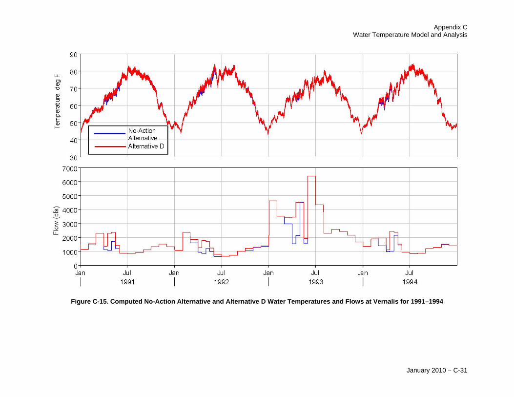
River flows and water temperature results for the SJR at Vernalis are plotted on Figure C-15. At this location, temperature predictions under Alternative D are affected by less cool water from New Melones Reservoir, warmer Stanislaus River water from increased heating in the Stanislaus River and increased flow in the SJR above the confluence from the recirculation flows. The temperature differences between the No-Action Alternative and the Alternative D results, evident in the spring of each year, are minor.

Figure C-16 shows the No-Action Alternative and Alternative D flows in Stanislaus River at Ripon and in the SJR at Vernalis. As this plot illustrates, the reductions in Stanislaus River flows require much larger recirculation flows to offset the loss of better quality Stanislaus River flows. Over the 4-year period shown in the plots, 1991 through 1994, the cumulative volume of water required for recirculation was nearly 400,000 acre-feet more than, or nearly 10 times as much as, the volume saved in New Melones Reservoir.



Figure C-15. Computed No-Action Alternative and Alternative D Water Temperatures and Flows at Vernalis for 1991–1994



Figure C-16. Computed No-Action Alternative and Alternative D Flows at Ripon and Vernalis



C.4 References AD Consultants, RMA, and Watercourse Engineering, Inc. 2006. Stanislaus–

Lower San Joaquin River Water Temperature Modeling and Analysis. Prepared for CALFED. CBDA Project No. ERP-02-P28. November.

AD Consultants, RMA, and Watercourse Engineering, Inc. 2007. Stanislaus–Lower San Joaquin River Water Temperature Modeling and Analysis. Prepared for CALFED. CBDA Project No. ERP-02-P28. April.

Bohan, J. P., and J. L. Grace, Jr. 1973. Selective Withdrawal from Man-made Lakes: Hydraulic Laboratory Investigation. Technical Report H-73-4. U.S. Army Corps of Engineers Waterways Experiment Station.

Hydrologic Engineering Center (HEC). 1998. HEC-5 Simulation of Flood Control and Conservation Systems, User’s Manual Version 8.0. U.S. Army Corps of Engineers, Hydrologic Engineering Center, Davis, CA.

Hydrologic Engineering Center (HEC). 1999. Water Quality Modeling of Reservoir System Operations Using HEC-5, Training Document. U.S. Army Corps of Engineers, Hydrologic Engineering Center, Davis, CA.

Hydrologic Engineering Center (HEC). 2001. HEC-5, Simulation of Flood Control and Conservation Systems, Appendix on Water Quality Analysis. U.S. Army Corps of Engineers, Hydrologic Engineering Center, Davis, CA.

Appendix C Water Temperature Model and Analysis 2 Appendices... · C.1.2 Planning Objectives ......

Documents

Transcript of Appendix C Water Temperature Model and Analysis 2 Appendices... · C.1.2 Planning Objectives ......