Appendix 15 - NTEPA€¦ · Appendix 15 Review of literature on sound in the ocean and on the...
140
Appendix 15 Review of literature on sound in the ocean and on the effects of noise on marine fauna
Transcript of Appendix 15 - NTEPA€¦ · Appendix 15 Review of literature on sound in the ocean and on the...

Appendix 15 Review of literature on sound in the ocean and on the effects of noise on marine fauna

4J:\Jobs\42906734\6 Deliverables\R1387 Underwater Noise Risk Assessment (URS)\R1387 Review of Literature on Sound in the Ocean FINAL 27 July 09.doc Ichthys Gas Field Development Project : Review of Literature on Sound in the Ocean and Effects of Noise on Marine Fauna
R E P O R T
Ichthys Gas Field Development Project : Review of Literature on Sound in the Ocean and Effects of Noise on Marine Fauna
Prepared for
INPEX Browse, Ltd. Level 22 100 St Georges Terrace PERTH WA 6000 Australia
27 July 2009
INPEX Document No. C036-AH-REP-0020 Rev 2
I C H T H Y S G A S F I E L D D E V E L O P M E N T P R O J E C T : R E V I E W O F L I T E R A T U R E O N S O U N D I N T H E O C E A N A N D E F F E C T S O F N O I S E
O N M A R I N E F A U N A
Prepared for INPEX Browse, Ltd., 27 July 2009
Project Manager:
John Polglaze Senior Principal Environmental Scientist
Project Director:
Ian Baxter Senior Principal Marine Environmental Scientist
URS Australia Pty Ltd
Level 3, 20 Terrace Road East Perth WA 6004 Australia T: 61 8 9326 0100 F: 61 8 9326 0296
Author:
Chris Coffey Project Environmental Scientist
Date: Reference: Status:
27 July 2009 42906734 – 1892: R1387 DK:M&C3050/PER Final
Recommended citation for this document is:
URS Australia Pty Ltd. 2009. Ichthys Gas Field Development Project: review of literature on sound in the ocean and on the effects of noise on marine fauna. Report prepared for INPEX Browse, Ltd., Perth, Western Australia.

I C H T H Y S G A S F I E L D D E V E L O P M E N T P R O J E C T : R E V I E W O F L I T E R A T U R E O N S O U N D I N T H E O C E A N A N D E F F E C T S O F N O I S E
O N M A R I N E F A U N A
Table of Contents
Prepared for INPEX Browse, Ltd., 27 July 2009
i
Table of Contents
1 Introduction ...................................................................................................... 1
1.1 Background ..................................................................................................................... 1 1.2 Objectives and Scope..................................................................................................... 1
2 Proposed Activity in Relation to Underwater Acoustic Impacts .................. 1
2.1 Marine infrastructure and associated activities .......................................................... 1 2.2 Noise generating activities ............................................................................................ 1 2.3 Environmental Setting within the Project Area............................................................ 1
2.3.1 Offshore development area .............................................................................. 1 2.3.2 Nearshore development area ........................................................................... 1
2.4 Important Marine Fauna in Respect of Noise Generation........................................... 1 2.4.1 Dugongs ........................................................................................................... 1 2.4.2 Turtles............................................................................................................... 1 2.4.3 Cetaceans......................................................................................................... 1 2.4.4 Saltwater crocodiles.......................................................................................... 1 2.4.5 Fish ................................................................................................................... 1
3 Physics of Underwater Sound......................................................................... 1
3.1 Nature of Sound and Hearing ........................................................................................ 1 3.2 Characterising and Measuring Sound .......................................................................... 1
3.2.1 Terminology ...................................................................................................... 1 3.2.2 Velocity ............................................................................................................. 1 3.2.3 Frequency, octaves and spectra ...................................................................... 1 3.2.4 Sound pressure and intensity levels................................................................. 1 3.2.5 Temporal properties of sound........................................................................... 1
3.3 Resonance ....................................................................................................................... 1 3.4 Blast and cavitation ........................................................................................................ 1 3.5 Sound Propagation and Transmission Loss................................................................ 1
3.5.1 Geometric spreading ........................................................................................ 1 3.5.2 Seawater absorption......................................................................................... 1 3.5.3 Scattering and other absorption losses ............................................................ 1 3.5.4 Propagation modelling and transmission anomalies ........................................ 1
4 Ambient Noise in the Ocean............................................................................ 1

I C H T H Y S G A S F I E L D D E V E L O P M E N T P R O J E C T : R E V I E W O F L I T E R A T U R E O N S O U N D I N T H E O C E A N A N D E F F E C T S O F N O I S E O N M A R I N E F A U N A
Table of Contents
ii
Prepared for INPEX Browse, Ltd., 27 July 2009
5 Natural Sources of Noise in the Ocean........................................................... 1
5.1 Characteristics of Natural Ambient Noise .................................................................... 1 5.2 Components of Natural Ambient Noise ........................................................................ 1
5.2.1 Eruptions, tremors and other tectonic events ................................................... 1 5.2.2 Ocean-wave interactions (microseisms)........................................................... 1 5.2.3 Lightning strikes................................................................................................ 1 5.2.4 Wind and rain sources ...................................................................................... 1 5.2.5 Thermal noise ................................................................................................... 1 5.2.6 Biological sources............................................................................................. 1
6 Anthropogenic Sources of Noise in the Ocean ............................................. 1
6.1 Components of Anthropogenic Noise .......................................................................... 1 6.2 General Shipping............................................................................................................. 1 6.3 Tugs.................................................................................................................................. 1 6.4 Dredges ............................................................................................................................ 1 6.5 Launches, Fishing Vessels and Powerboats ............................................................... 1 6.6 Petroleum Industry Operations ..................................................................................... 1 6.7 Pile Driving....................................................................................................................... 1 6.8 Rock and dredge spoil dumping ................................................................................... 1 6.9 Drilling .............................................................................................................................. 1 6.10 Blasting ............................................................................................................................ 1 6.11 Pipelines........................................................................................................................... 1
6.11.1 Pipelaying ......................................................................................................... 1 6.11.2 Pipe operations................................................................................................. 1
7 Behavioural and Physiological Effects of Noise............................................ 1
7.1 Auditory System of Marine Fauna................................................................................. 1 7.1.1 Cetaceans......................................................................................................... 1 7.1.2 Sirenians ........................................................................................................... 1 7.1.3 Marine turtles .................................................................................................... 1 7.1.4 Crocodiles ......................................................................................................... 1 7.1.5 Sharks............................................................................................................... 1 7.1.6 Fish ................................................................................................................... 1
7.2 Categories of Sound Impacts ........................................................................................ 1

I C H T H Y S G A S F I E L D D E V E L O P M E N T P R O J E C T : R E V I E W O F L I T E R A T U R E O N S O U N D I N T H E O C E A N A N D E F F E C T S O F N O I S E
O N M A R I N E F A U N A
Table of Contents
Prepared for INPEX Browse, Ltd., 27 July 2009
iii
7.2.1 Zones of influence ............................................................................................ 1 7.2.2 Zone of audibility............................................................................................... 1 7.2.3 Zone of behavioural responses ........................................................................ 1 7.2.4 Zone of potential masking ................................................................................ 1 7.2.5 Zone-inducing possible temporary threshold shifts in hearing ......................... 1 7.2.6 Zone-inducing possible permanent threshold shift or other tissue damage..... 1
7.3 Synthesis of Anthropogenic Noise Impacts and Physiological and Behavioural effects upon Marine Mammals....................................................................................... 1 7.3.1 State of Current Knowledge ............................................................................. 1 7.3.2 Noise Exposure Criteria.................................................................................... 1 7.3.3 Exposure Criteria for Injury............................................................................... 1 7.3.4 Exposure Criteria for Behaviour ....................................................................... 1 7.3.5 Conclusion ........................................................................................................ 1
8 Effects of Noise on Marine Fauna................................................................... 1
8.1 Dredging .......................................................................................................................... 1 8.2 Pile Driving ...................................................................................................................... 1 8.3 Shipping Noise ................................................................................................................ 1 8.4 Vessel Presence.............................................................................................................. 1 8.5 Rock Dumping and Dredge Spoil Disposal .................................................................. 1 8.6 Seismic Surveys.............................................................................................................. 1
8.6.1 Vertical seismic profiling ................................................................................... 1 8.7 Drilling.............................................................................................................................. 1 8.8 Explosives ....................................................................................................................... 1
8.8.1 Marine Mammals .............................................................................................. 1 8.8.2 Fish ................................................................................................................... 1 8.8.3 Marine Turtles................................................................................................... 1
8.9 Pipeline Laying and Operation ...................................................................................... 1
9 References........................................................................................................ 1
10 Limitations ........................................................................................................ 1

I C H T H Y S G A S F I E L D D E V E L O P M E N T P R O J E C T : R E V I E W O F L I T E R A T U R E O N S O U N D I N T H E O C E A N A N D E F F E C T S O F N O I S E O N M A R I N E F A U N A
Tables, Figures, Drawings, Appendices
iv
Prepared for INPEX Browse, Ltd., 27 July 2009
Tables, Figures, Drawings, Appendices
Tables
Table 3-1 Sounds Grouped by Temporal Character ........................................................................................ 1 Table 3-2 Sound transmission loss rates by pure cylindrical and spherical spreading from a nominal source
of 200 dB (re 1 µPa)......................................................................................................................... 1 Table 3-3 Seawater absorption loss rates for different frequencies at 5º C..................................................... 1 Table 5-1 Examples of intense natural sound sources .................................................................................... 1 Table 6-1 Typical frequency ranges of anthropogenic noise sources.............................................................. 1 Table 6-2 Comparison of sound source levels from a range of anthropogenic sound sources....................... 1 Table 6-3 Summary of noise sources and activities associated with oil and gas exploration and production. 1 Table 6-4 Summary of noise sources and activities which may be associated with pipelaying ...................... 1 Table 7-1 Citations of selected studies examining the effects of exposure to sound on fishes that have most
relevance to pile driving. .................................................................................................................. 1 Table 7-2 Summary characteristics of some common human sound sources ................................................ 1 Table 7-3 Features of an audible source likely to increase level of attention and invoke behavioural
responses in marine fauna............................................................................................................... 1 Table 7-4 Type and possible consequences of behaviour changes from exposure to human noise source*. 1 Table 7-5 Functional marine mammal hearing groups, auditory bandwidth (estimated lower to upper
frequency hearing cut-off), genera represented in each group, and group-specific (M) frequency weightings ........................................................................................................................................ 1
Table 7-6 Sound types, acoustic characteristics and selected examples of anthropogenic sound sources ... 1 Table 7-7 Proposed injury criteria for individual marine mammals exposed to 'discrete' noise events, either
single or multiple exposures within a 24-h period ............................................................................ 1 Table 7-8 Functional marine mammal hearing groups, auditory bandwidth (estimated lower to upper
frequency hearing cut-off); genera represented in each group, and group specific (M) frequency-weightings ........................................................................................................................................ 1
Table 8-1 Attenuation of acoustic signal from vertical seismic profiling........................................................... 1 Table 8-2 Peak pressure (kPa) at distance from underwater (surface) blast................................................... 1 Table 8-3 Peak pressure (kPa) at distance from underwater (confined) blast................................................. 1
Figures
Figure 1-1 Offshore development area.............................................................................................................. 1 Figure 1-2 Ichthys Field ..................................................................................................................................... 1 Figure 1-3 Darwin Harbour and the nearshore development area.................................................................... 1 Figure 3-1 Shapes of natural sine and electronically generated square and pulse waves ............................... 1 Figure 3-2 Wave phase and interference .......................................................................................................... 1

I C H T H Y S G A S F I E L D D E V E L O P M E N T P R O J E C T : R E V I E W O F L I T E R A T U R E O N S O U N D I N T H E O C E A N A N D E F F E C T S O F N O I S E
O N M A R I N E F A U N A
Tables, Figures, Drawings, Appendices
Prepared for INPEX Browse, Ltd., 27 July 2009
v
Figure 3-3 Measuring sound amplitude..............................................................................................................1 Figure 3-4 Spectrum showing the broadband source from detonating ~0.45 kg (1 lb) of high explosive at
37 m depth ........................................................................................................................................1 Figure 3-5 Diagrammatic representation of the zone of bulk cavitation.............................................................1 Figure 3-6 Schematic of the mechanism forming the deep sound channel .......................................................1 Figure 3-7 Simplified schematic showing sound paths from surface and deep sources, and highlighting the
transmission and loss process for a surface source (not all paths shown) ......................................1 Figure 3-8 Depth profiles showing sound transmission losses in different ocean regimes, as predicted by a
parabolic equation model (MMPE) for a low frequency (200 Hz) and high frequency (3 kHz) source at 50 m depth ........................................................................................................................1
Figure 3-9 Seawater absorption coefficients for three temperatures at zero depth, 35.2 PSU (salinity) and pH 8...................................................................................................................................................1
Figure 4-1 Generalised ambient noise spectra attributable to various sources .................................................1 Figure 4-2 Pressure density curves of ambient noise components ...................................................................1 Figure 5-1 Triangular shaped low frequency signal from subsea earthquake ...................................................1 Figure 5-2 Colour spectrograms showing examples of T-waves .......................................................................1 Figure 5-3 Frequency of events during the Gorda (top) and Coaxial segment (bottom) episodes....................1 Figure 5-4 A 900 second (15 minute) portion of the 'Inferred Harmonic Tremor' that was detected south of
Japan on many separate occasions in 1998-2000. ..........................................................................1 Figure 5-5 600 second (10 minute) spectrogram showing whale calls recorded by the West Atlantic SOSUS
array during and after a subsea earthquake.....................................................................................1 Figure 5-6 Spectrogram of an underwater recording of a lightning strike ..........................................................1 Figure 5-7 Global distribution of lightning flash density (km2) per annum..........................................................1 Figure 5-8 Australian annual lightning ground flash density ..............................................................................1 Figure 5-9 Underwater spectrograms.................................................................................................................1 Figure 5-10 Average monthly rainfall for Darwin (mm).........................................................................................1 Figure 5-11 Frequency range for some baleen whales and dolphins ..................................................................1 Figure 6-1 Merchant ship acoustic signatures measured in Dampier (WA) by DSTO.......................................1 Figure 6-2 Vessel traffic density around Australia indicated via daily vessel movement reports (VMRs) to the
Australian Maritime Safety Authority (AMSA) ...................................................................................1 Figure 6-3 Annual number of vessels visiting the port of Darwin .......................................................................1 Figure 6-4 Sources and causes of underwater noise associated with the oil and gas industries......................1 Figure 7-1 Hearing and sound production structures in the dolphin ..................................................................1 Figure 7-2 Measuring inner anatomy and determining and audiogram using a CT scanner.............................1 Figure 7-3 Zones of influence.............................................................................................................................1

I C H T H Y S G A S F I E L D D E V E L O P M E N T P R O J E C T : R E V I E W O F L I T E R A T U R E O N S O U N D I N T H E O C E A N A N D E F F E C T S O F N O I S E O N M A R I N E F A U N A
Tables, Figures, Drawings, Appendices
vi
Prepared for INPEX Browse, Ltd., 27 July 2009
Figure 7-4 Plot indicating sound exposure regimes (s) and energy flux densities (b) that can induce measurable TTS in odontocetes ...................................................................................................... 1
Figure 7-5 PCAD model..................................................................................................................................... 1

I C H T H Y S G A S F I E L D D E V E L O P M E N T P R O J E C T : R E V I E W O F L I T E R A T U R E O N S O U N D I N T H E O C E A N A N D E F F E C T S O F N O I S E
O N M A R I N E F A U N A
Introduction Section 1
Prepared for INPEX Browse, Ltd., 27 July 2009
7
1 Introduction
1.1 Background INPEX Browse, Ltd. (INPEX) proposes to develop the natural gas and associated condensate contained in the Ichthys Field in the Browse Basin at the western edge of the Timor Sea about 200 km off Western Australia’s Kimberley coast. The field is about 850 km west south west of Darwin in the Northern Territory (Figure 1-1) and encompasses an area of approximately 800 km2 (out of the 3041 km2 in the permit area) with water depths ranging from 90 to 340 m (Figure 1-2).
The two reservoirs which make up the field are estimated to contain 12.8 tcf (trillion cubic feet) of sales gas and 527 MMbbl (million barrels) of condensate. INPEX will process the gas and condensate to produce liquefied natural gas (LNG), liquefied petroleum gas (LPG) and condensate for export to overseas markets.
For the Ichthys Gas Field Development Project (the Project), the company plans to install offshore facilities for the extraction of the natural gas and condensate at the Ichthys Field and a subsea gas pipeline from the field to onshore facilities at Blaydin Point in Darwin Harbour in the Northern Territory (Figure 1-3). A two train LNG plant, an LPG fractionation plant, a condensate stabilisation plant and a product loading jetty will be constructed at a site zoned for development on Blaydin Point. Around 85% of the condensate will be extracted and exported directly from the offshore facilities while the remaining 15% will be processed at and exported from Blaydin Point.
In May 2008 INPEX referred its proposal to develop the Ichthys Field to the Commonwealth’s Department of the Environment, Water, Heritage and the Arts and the Northern Territory’s Department of Natural Resources, Environment and the Arts. The Commonwealth and Northern Territory ministers responsible for environmental matters both determined that the Project should be formally assessed at the environmental impact statement (EIS) level to ensure that potential impacts associated with the Project are identified and appropriately addressed.
Assessment will be undertaken in accordance with the Environment Protection and Biodiversity Conservation Act 1999 (Cwlth) (EPBC Act) and the Environmental Assessment Act (NT) (EA Act). It was agreed that INPEX should submit a single EIS document to the two responsible government departments for assessment.
For the purposes of this report, the Project has been divided into two main components:
• Offshore development area—including the Ichthys Field in the offshore waters of north-western Australia as well as the subsea pipeline route from the field to the mouth of Darwin Harbour (Figure 1-1).
• Nearshore development area—including from the mouth of Darwin Harbour south to the coastal waters around Blaydin Point and Middle Arm Peninsula (Figure 1-3).

I C H T H Y S G A S F I E L D D E V E L O P M E N T P R O J E C T : R E V I E W O F L I T E R A T U R E O N S O U N D I N T H E O C E A N A N D E F F E C T S O F N O I S E O N M A R I N E F A U N A
Section 1 Introduction
8
Prepared for INPEX Browse, Ltd., 27 July 2009
Figure 1-1 Offshore development area
Figure 1-2 Ichthys Field

I C H T H Y S G A S F I E L D D E V E L O P M E N T P R O J E C T : R E V I E W O F L I T E R A T U R E O N S O U N D I N T H E O C E A N A N D E F F E C T S O F N O I S E
O N M A R I N E F A U N A
Introduction Section 1
Prepared for INPEX Browse, Ltd., 27 July 2009
9
Figure 1-3 Darwin Harbour and the nearshore development area
1.2 Objectives and Scope Activities associated with the offshore development, and nearshore activities including the construction of a product loading jetty and other project associated activities within Darwin Harbour will generate noise, which has the potential to lead to adverse impacts upon marine fauna in the vicinity of these activities. Some noise-generating activities will also continue through the operations and maintenance phases of the project.
Sources of noise will include pile driving, dredging and trenching activities, rock armour and dredge spoil dumping, general vessel traffic, pipelaying activities, drilling, vertical seismic profiling and blasting. All of these activities may disturb marine fauna to varying degrees. As a result, it was deemed pertinent to undertake a

I C H T H Y S G A S F I E L D D E V E L O P M E N T P R O J E C T : R E V I E W O F L I T E R A T U R E O N S O U N D I N T H E O C E A N A N D E F F E C T S O F N O I S E O N M A R I N E F A U N A
Section 1 Introduction
10
Prepared for INPEX Browse, Ltd., 27 July 2009
review of the literature on the effects of noise on marine fauna and potential impacts associated with this project.
This report provides information on important marine fauna within Darwin Harbour and the offshore development area in relation to noise generating activities and examines the potential impacts associated with noise generated from activities attendant to this project. The report also provides a literature review on sound in the ocean and the effects of noise on marine fauna, where the following topics are discussed:
• Noise sources associated with the project
• The physics of underwater sound
• The characteristics of ambient noise
• Natural sources of noise in the ocean
• Anthropogenic sources of noise in the ocean
• Categories of noise effects on marine fauna
• effects of noise generation on marine fauna.
This review focuses principally on the known and potential physiological and behavioural responses of fauna to noise in the offshore marine environment, with emphasis given to Darwin Harbour where information is available. Although this review is not exhaustive, it does illustrate and place into context the range of impacts that might be anticipated as a result of underwater noise generated by this project.
The review’s weighting towards cetaceans is a reflection of the relatively high research intensity afforded to this group of animals. Very little is known about the effects of exposure to sounds on other marine fauna such as sirenians, turtles, fishes, etc. In cases where data are available, they are so few that one must be cautious in attempting to extrapolate between species, even for identical stimuli. Moreover, caution also needs to be exercised with any attempts to extrapolate results between stimuli because the characteristics of sources (e.g. ship noise, pile-driving) differ significantly from one another.
I C H T H Y S G A S F I E L D D E V E L O P M E N T P R O J E C T : R E V I E W O F L I T E R A T U R E O N S O U N D I N T H E O C E A N A N D E F F E C T S O F N O I S E
O N M A R I N E F A U N A
Proposed Activity in Relation to Underwater Acoustic Impacts Section 2
Prepared for INPEX Browse, Ltd., 27 July 2009
11
2 Proposed Activity in Relation to Underwater Acoustic Impacts
2.1 Marine infrastructure and associated activities Marine infrastructure to be installed and associated activities within the nearshore and offshore areas is summarised below.
Offshore development area
Components of the Project that will be developed in the offshore area include subsea production wells and flowlines, a central processing facility (CPF), floating production storage and offloading (FPSO) facility and the major portion of the subsea gas export pipeline. Details of all offshore infrastructures are summarised as follows:
• Drilling of production wells via a mobile offshore drilling unit (MODU) and support vessels.
• Installation of approximately 50 subsea wells and flowlines to carry the natural gas and reservoir fluids from the wells to the CPF.
• Installation and commissioning of the CPF, FPSO and gas export pipeline.
• Export of condensate via FPSO to offtake tankers.
• On-going operation of the CPF, FPSO and gas export pipeline.
• Decommissioning.
Nearshore development area
Infrastructure to be constructed in this area includes a product offloading jetty with a marine outfall, a module offloading facility, shipping and navigation channels, and the nearshore section of the gas export pipeline with a shore crossing south of Wickham Point. Details of all nearshore infrastructure can be summarised as follows:
• Construction of the nearshore portion of the gas export pipeline, including trenching, rock armouring and pipeline shore crossing.
• Construction of a jetty and module offloading facility, with associated dredging for shipping and navigation channels.
• Operation of the jetty for hydrocarbon export, and operation of the module offloading facility.
• Operation of the marine outfall on the jetty.
• Decommissioning.
2.2 Noise generating activities Construction and associated activities associated with the offshore and nearshore development areas will result in a temporary increase in noise levels and a change in the characteristics of ambient background noise. These alterations could affect transitory and resident marine fauna within the vicinity of these activities.

I C H T H Y S G A S F I E L D D E V E L O P M E N T P R O J E C T : R E V I E W O F L I T E R A T U R E O N S O U N D I N T H E O C E A N A N D E F F E C T S O F N O I S E O N M A R I N E F A U N A
Section 2 Proposed Activity in Relation to Underwater Acoustic Impacts
12
Prepared for INPEX Browse, Ltd., 27 July 2009
Specific activities which will generate noise are:
1. dredging and trenching
2. pile driving
3. rock armour dumping and dredge spoil dumping
4. general shipping/vessel traffic (pre and post construction)
5. drilling
6. underwater blasting
7. subsea pipelaying.
At present there is no information available on actual noise levels likely to be generated from this project, or the exact frequency and duration of these noise generating activities as well as the time of year these activities are likely to occur. The only guidance available is that construction of the Project is likely to take approximately two years in total, with at least some activities likely to occur on a 24 hours a day basis (e.g. dredging).
2.3 Environmental Setting within the Project Area 2.3.1 Offshore development area The Ichthys Field is located approximately 200 km from the Kimberly coast, Western Australia, in the northern Browse Basin in petroleum exploration permit area WA 285 P R1 (see Figure 1-1). The offshore waters of the Ichthys Field are between 235 m and 275 m deep (see Figure 1-2). Browse Island is located 30 km south of the field, and Echuca Shoal is 50 km to the east. The continental shelf is located around 20 km to the west of the Ichthys Field.
The subsea pipeline route extends from the Ichthys Field to the mouth of Darwin Harbour, a distance of around 900 km. Most of this alignment is distant from land, with the exception of the eastern end of the route that curves around the Cox Peninsula as it leads into Darwin Harbour. The pipeline runs in the vicinity of the North Australia Exercise Area (NAXA), used by the Australian Defence Force, in the eastern portion of the route.
2.3.2 Nearshore development area The nearshore pipeline route extends from the mouth of Darwin Harbour, through the centre of the Harbour to the low tide level at the pipeline shore crossing area south of Wickham Point, in Middle Arm near Channel Island (see Figure 1-3). The pipeline route for the Ichthys Project runs parallel to the existing Bayu-Undan pipeline, utilised by the ConocoPhillips Darwin LNG plant. Other seabed features near the pipeline route include Karumba Shoal, Plater Rock and Weed Reef, to the west of the alignment. Channel Island is located just west of the Middle Arm Peninsula, around 1.5 km south of the pipeline shore crossing.
The nearshore development area also includes the marine environment around Blaydin Point, below the low tide mark. This area is located on the southern banks of East Arm, downstream of the Elizabeth River. The existing East Arm Port is located on the northern side of East Arm. Features of this area include South Shell Island and Old Man Rock. Also, west of Blaydin Point on the Middle Arm Peninsula are two narrow tidal creeks known as Lightning Creek and Cossack Creek, which are both used for recreational fishing.

I C H T H Y S G A S F I E L D D E V E L O P M E N T P R O J E C T : R E V I E W O F L I T E R A T U R E O N S O U N D I N T H E O C E A N A N D E F F E C T S O F N O I S E
O N M A R I N E F A U N A
Proposed Activity in Relation to Underwater Acoustic Impacts Section 2
Prepared for INPEX Browse, Ltd., 27 July 2009
13
Darwin Harbour is a large ria system, or drowned river valley, with an area of about 500 km2. In its southern and south-eastern portions the Harbour has three main components (East, West and Middle arms) that merge into a single unit, along with the smaller Woods Inlet, before joining the open sea. Freshwater inflow to the Harbour occurs from January to April, when estuarine conditions prevail in all areas (Hanley 1988).
The main channel of the Port of Darwin is around 15-25 m deep, with a maximum depth of 36 m (Figure 3-12). The channel favours the eastern side of the Harbour, with broader shallower areas occurring on the western side. Intertidal flats and shoals are generally more extensive on the western side of the Harbour than on the eastern side. The channel continues into East Arm, towards Blaydin Point, at water depths of greater than 15 m LAT; the bathymetry in this area has been modified by dredging for the development of East Arm Port. A slightly deeper channel extends into Middle Arm, up to the western side of Channel Island. A shallower channel (generally 10 to 15 m LAT depth) separates Wickham Point from Channel Island and terminates in Jones Creek
Water quality in Darwin Harbour is generally high, although naturally turbid most of the time. Water quality parameters vary greatly with the tide (spring versus neap), location of sampling (inner versus outer Harbour), and with the season (wet season versus dry season). The Darwin wet season extends from November to March and its effects on Harbour water quality (due to high surface runoff from the land) can last until April or May depending on rainfall. Dry season climate conditions prevail from May to September.
Darwin Harbour is characterised by a macrotidal regime. Tides are predominantly semidiurnal (two highs and two lows per day), with a slight inequality between the successive tides during a single day. For a two day period during neaps, there are nearly diurnal tide conditions. The lowest spring tides of the year occur during October, November and December. Mean sea level is approximately 4.0 m above LAT. Spring tides can produce tidal ranges of up to 7.5 m (0.0 m above LAT at low tide to 7.5 m above LAT at high tide), while the neap tide range can be as low as 1.4 m (3.1 above LAT at low tide to 4.5 m above LAT at high tide) (URS 2009).
Tides have a marked effect on water clarity in the Harbour, with waters of neap tides being the clearest, while spring tides carry a lot of sediment from the fringing mangroves (DHAC 2007). The areas with the highest natural sedimentation are in the upper reaches of East and Middle arms. Medium levels of sedimentation occur in the seaward end of West Arm and the lowest levels are in the more open water areas such as East Arm Wharf, Larrakeyah and the seaward boundary (DHAC 2006). It is estimated that 60% of the Harbour’s sediments originate from offshore. The remainder is input via rivers and creeks, derived predominantly from erosion of channel walls. Direct contribution to the Harbour from sheet erosion is likely to be limited because of the very low hillslope gradients adjacent to the Harbour (DHAC 2006).
With its tropical location, water temperatures in Darwin Harbour are typically high, but some seasonal variations do occur. Water temperatures are lowest (23 ˚C) in June-July and highest (33 ˚C) in October-November (Padovan 1997).
Darwin Harbour contains variable bottom sediments, which can be divided into four types
• terrigenous gravels, which occur primarily in the main channel
• calcareous sands with greater than 50% biogenic carbonate, which are among or close to the small coral communities at East Point, Lee Point and Channel Island. Carbonate sediments, largely derived from molluscan shell fragments, also occur in spits and shoals close to the Harbour mouth
I C H T H Y S G A S F I E L D D E V E L O P M E N T P R O J E C T : R E V I E W O F L I T E R A T U R E O N S O U N D I N T H E O C E A N A N D E F F E C T S O F N O I S E O N M A R I N E F A U N A
Section 2 Proposed Activity in Relation to Underwater Acoustic Impacts
14
Prepared for INPEX Browse, Ltd., 27 July 2009
• terrigenous sands on beaches and spits, with 10–50% carbonate, largely derived from molluscs. This type of sediment is predominantly quartz and clay
• mud and fine sand on broad, gently inclined intertidal mudflats that occur in areas characterised by low current and tidal velocities, such as in Kitchener Bay (prior to the construction of the Darwin City Waterfront).
Salinity in Darwin Harbour varies considerably during the year, particularly in East, Middle and West arms where freshwater influence is greatest during the wet season. Seawater has a global average salinity of 35 parts per thousand (ppt) (DEH 2008). Salinities throughout the Harbour however are about 37 ppt during the dry season, with surface and bottom depths having similar levels. Salinity tends to be higher in the dry season owing to increased evaporation and less fresh water inflow. At the height of monsoonal inflow during February March, areas in the middle of the Harbour such as Weed Reef can experience salinity levels of 27 ppt (Parry & Munksgaard 1995). The variable low levels of salinity within Darwin Harbour will have a marked attenuation effect on acoustic propagation. The temporal and spatial variability of salinity within Darwin Harbour also creates difficulties in accurately predicting acoustic propagation.
2.4 Important Marine Fauna in Respect of Noise Generation 2.4.1 Dugongs Dugongs (Dugong dugon) are listed marine and migratory species under the Commonwealth Environment Protection and Biodiversity Conservation Act 1999 (EPBC Act)
The dugong has a range that extends from east Africa to the western Pacific. In Australia, dugongs are distributed along the northern coastline from Shark Bay in Western Australia to Moreton Bay near Brisbane, Queensland (NRETAS 2008b).
Dugongs are herbivorous and demonstrate a strong dietary preference for seagrasses, though they will also eat algae (Anderson 1982; Marsh 1999; Marsh et al. 2002). Dugongs are usually found in coastal areas such as shallow protected bays, mangrove channels and the lee of large inshore islands where seagrass grows (Heinsohn, Marsh & Anderson 1979). However, they have also been recorded further offshore in areas where the continental shelf is wide, shallow (up to 37 m deep) and protected (Marsh et al. 2002; Lee Long, Mellors & Coles 1993).
Given that water depths in the offshore development area range from 190-250 m, the presence of feeding habitat for dugongs is non existent, as seagrass or macro algae could not grow at these depths, although migrating animals may pass through the area. During vessel surveys only one dugong was observed in the vicinity of the Ichthys Field. Dugongs were recorded more commonly in aerial and vessel-based surveys throughout the coastal survey areas, around Camden Sound and Pender Bay, and were also observed several kilometres off the north-east coast of North Maret Island and near South Beach, South Maret Island (RPS 2007b).
Within Northern Territory waters, dugongs occur in the Gulf of Carpentaria and Arnhem Land with fewer on the western coast of the territory (NRETAS 2008b). Areas identified as key sites for the conservation of dugong and seagrass habitat include the north coast of the Tiwi Islands, Coburg Peninsula, and Blue Mud Bay, Limmen Coast and the Sir Edward Pellew Group of islands on the east Arnhem Land coast (URS 2009). Aerial surveys in the Anson-Beagle Bioregion have recorded large numbers of dugongs around the Vernon Islands and Gunn Point, 30-50 km north east of Darwin Harbour. Satellite tracking data showed that dugongs can move

I C H T H Y S G A S F I E L D D E V E L O P M E N T P R O J E C T : R E V I E W O F L I T E R A T U R E O N S O U N D I N T H E O C E A N A N D E F F E C T S O F N O I S E
O N M A R I N E F A U N A
Proposed Activity in Relation to Underwater Acoustic Impacts Section 2
Prepared for INPEX Browse, Ltd., 27 July 2009
15
large distances and dugongs tagged around the Vernon Islands spent time in Darwin Harbour, around the Tiwi Islands and as far west as Cape Scott and Cape Ford south of the Peron Islands, 100-120 km south west of Darwin Harbour (Whiting 2003).
Dugongs are known to occur in Darwin Harbour waters, albeit in relatively low numbers. Dugongs have been recorded in high densities at Gunn Point and the Vernon Islands, approximately 30-50 km north-east of the mouth of the Harbour. The species is also known to travel long distances (Whiting 2003).
Dugongs have been observed foraging on the rocky reef flats between Channel Island and the western end of Middle Arm Peninsula, in a three-year study conducted by Charles Darwin University and Biomarine International. Dugongs were observed in this area during most months of the year, except from September to December. No seagrass occurs on the reef flat in this area—instead, the dugongs were likely to have been feeding on macro algae (Whiting 2001).
Whiting (2001) suggests that the occurrence of small, sparse patches of seagrass in the Anson-Beagle Bioregion may cause dugongs to supplement their diet with algae. Dugongs had been observed foraging on algae on similar reefs in Fog Bay, 60 km south-west of Darwin Harbour (Whiting 2001).
2.4.2 Turtles Six species of marine turtle are known to occur in the Northern Territory waters; the loggerhead turtle (Caretta caretta), green turtle (Chelonia mydas), leatherback (Dermochelys coriacea), hawksbill (Eretmochelys imbricata), Pacific/olive ridley (Lepidochelys olivacea) and flatback turtle (Natator depressus). All of these species are listed marine and migratory species under the EPBC Act. The loggerhead, leatherback and Pacific/olive ridley are listed as endangered, while the remaining species are listed as vulnerable. The green, hawksbill and flatback turtles occur in Darwin Harbour regularly, and the olive ridley and loggerhead turtles are suspected to be infrequent users. The leatherback turtle is considered an oceanic species and is unlikely to occur in Darwin Harbour (Whiting 2001).
The shoreline throughout Darwin Harbour, and particularly in Middle Arm and East Arm, largely consists of mangroves and mud flats and does not provide suitable nesting habitat for any species of turtle that may frequent the area (URS 2009). Turtles visiting the Harbour are more likely to be foraging for food.
Green turtles are predominantly herbivorous and feed on seagrasses and algae. Immature and adult size green turtles have been observed in a variety of habitats throughout Darwin Harbour feeding on sparse seagrass, algae and mangrove seedlings and fruits (Whiting 2003; Metcalfe 2007). Published records include observations of relatively high numbers of green turtles foraging on the intertidal reef flats between Channel Island and the Middle Arm Peninsula, particularly in the dry season when algae are more abundant (Whiting 2001). In the offshore area, green turtles are known to nest at Browse Island.
Hawksbill turtles are omnivores but in some areas they are reported as sponge specialists. In Darwin Harbour, immature and adult sized Hawksbill turtles have been reported using rocky reef habitat at Channel Island, but they may also occur in other habitats (Whiting 2001). Hawksbill turtles occur in Darwin Harbour at lower abundances than green turtles, with around four times as many green turtles recorded at the Channel Island foraging area than hawksbill turtles (Whiting 2001).
While flatback turtles are the most commonly encountered nesting species in the Anson-Beagle Bioregion (Chatto & Baker 2008), the species appears to occur in Darwin Harbour rarely, with no nesting activity inside the
I C H T H Y S G A S F I E L D D E V E L O P M E N T P R O J E C T : R E V I E W O F L I T E R A T U R E O N S O U N D I N T H E O C E A N A N D E F F E C T S O F N O I S E O N M A R I N E F A U N A
Section 2 Proposed Activity in Relation to Underwater Acoustic Impacts
16
Prepared for INPEX Browse, Ltd., 27 July 2009
Harbour and only occasional observations of flatback turtles swimming and foraging (Whiting 2001). Likewise, olive Ridley and loggerhead turtles are rarely observed in Harbour waters (Whiting 2003).
2.4.3 Cetaceans All cetaceans are protected under the EPBC Act. Cetaceans that occur within the North West Shelf and Oceanic Shoals bioregions include a variety of baleen whales and toothed whales including dolphins. There are other species of cetaceans that may occur in the vicinity of the offshore development area based on knowledge of their general distribution and biology, although they have not been recorded in the area in any surveys. These species are included in the discussion below.
The most commonly recorded cetacean species in Darwin Harbour are three coastal dolphins—the Australian snubfin (Orcaella heinsohni), the Indo-Pacific humpback (Sousa chinensis) and the Indo-Pacific bottlenose (Tursiops aduncus) (Palmer 2008). Other cetaceans that have been recorded in Darwin Harbour include the great sperm whale (Physeter macrocephalus), the pygmy sperm whale (Kogia simus) and the humpback whale (Megaptera novaenglie). However, recordings of these species are rare and may represent vagrant individual sightings. Occasional pods of false killer whales (Pseudorca crassidens) are known to visit the Harbour but little research has been conducted into their utilisation of the area (URS 2009). While the blue whale (Balaenoptera musculus) is listed as a potential inhabitant according to the public threatened species database (DEWHA 2008), it is extremely unlikely to occur in Darwin Harbour and has not been recorded.
Whales
Baleen whales
Humpback whales
Humpback whales are the most common whale species observed in the North West Shelf Bioregion, and are seasonally abundant between August and October. They are a listed as vulnerable and a migratory species under the EPBC Act.
Australia has two discrete populations of humpback whales—one migrating along the west coast and the other migrating along the east coast. The humpback whale stock that winters off Western Australia is known as the Group IV (Breeding Stock D) population (Jenner, Jenner & McCabe 2001), and is thought to have a total population of between 30 000 and 38 000 whales (Branch 2006).
Stock D humpback whales migrate annually from their Antarctic feeding grounds to their breeding and calving areas off the Kimberley coast. The known calving area for Stock D humpback whales covers approximately 23 000 km2 from the Lacepede Islands in the south to Adele Island in the north and to Camden Sound in the east (Jenner, Jenner & McCabe 2001). Calving occurs between June and November, with the peak of the southbound migration between late August and early September; cows and calf pairs trail the main migratory movement by three to four weeks (Chittleborough 1965).
There is no evidence that the offshore development area is a calving ground for humpback whales, although the nearshore waters of the Kimberley Bioregion are known to be used by humpbacks for calving and resting. Humpback whale densities recorded in field surveys were significantly higher in Camden Sound and Pender Bay than in the Browse Basin. Whales observed in Pender Bay exhibited surface passive behaviour suggesting that the area is used for resting. Cow–calf pods appear to congregate in the area between Pender Bay and the Lacepede Islands during mid-September, using the area as a staging point and resting place prior to beginning their southern migration (RPS 2007b).

I C H T H Y S G A S F I E L D D E V E L O P M E N T P R O J E C T : R E V I E W O F L I T E R A T U R E O N S O U N D I N T H E O C E A N A N D E F F E C T S O F N O I S E
O N M A R I N E F A U N A
Proposed Activity in Relation to Underwater Acoustic Impacts Section 2
Prepared for INPEX Browse, Ltd., 27 July 2009
17
Blue whales
Two subspecies of blue whale are found in the southern hemisphere; the “true” blue whale (Balaenoptera musculus intermedia) and the pygmy blue whale (Balaenoptera musculus brevicauda). The blue whale is listed as endangered and a migratory species under the EPBC Act.
Pygmy blue whales have been observed on many occasions during the winter months in locations such as the Savu Sea west of Timor (URS 2009) and have been recorded along the coast of Western Australia as far north as Cape Londonderry (URS 2009). While pygmy blue whales have been recorded in the Kimberley region, true blue whales are uncommon north of 60 °S (Branch et al. 2007).
Pygmy blue whales are assumed to breed in the tropical north, like other rorquals. Previous studies on the distribution of pygmy blue whales and true blue whales in the southern hemisphere suggest that the Western Australian continental slope is a likely migratory path between a southern feeding area and a northern calving area. The location of the northern breeding ground is thought to be in deep waters to the west of the Browse Basin (McCauley 2009). There is no current consensus on the size of the pygmy blue whale population (DEH 2005), however in 1996 the Australian Nature Conservation Agency estimated there to be 6000 animals (Bannister, Kemper & Warneke 1996).
No true blue whales or pygmy blue whales were observed in vessel surveys of the offshore development area, although pygmy blue whale songs were recorded on the acoustic logger during October 2006. The pygmy blue whale song comprised at least two calling animals-as not all individuals vocalise, this suggests that several whales could have been in the area at that time (RPS 2007b).
Minke whales
Antarctic minke whales (Balaenoptera bonaerensis) are a listed migratory species under the EPBC Act. They appear to migrate from summer southern feeding grounds to northern tropical feeding grounds in the winter months. However, the detailed pattern of migration is still unclear and may be quite complex. In the north east Pacific, for instance, it has been suggested that some minke whales are migratory while others form a resident population. In Australia, it is known that dwarf minke whales (Balaenoptera acutorostrata unnamed subsp.) occur broadly from Victoria to northern Queensland between March and October, with the maximum number of sightings on the northern Great Barrier Reef in June and July.
A small number of minke whales (seven) were recorded in the offshore development area during vessel surveys. One was positively identified as the dwarf subspecies.
Toothed whales and dolphins
Offshore area
Information on toothed whale and dolphin species off the Kimberley coast is limited, especially in offshore waters. In total, 21 species of toothed whale and dolphin could occur in the offshore development area (DEWHA 2008). Species recorded by Jenner, Jenner and McCabe (2001) in the Kimberley region included false killer whales (Pseudorca crassidens), dwarf spinner dolphins, spinner dolphins (Stenella longirostris), bottlenose dolphins (Tursiops sp.) and Australian snubfin dolphins (Orcaella heinsohni). Sperm whales (Physeter macrocephalus) have also been recorded in the Kimberley (Townsend 1935). Fifteen species of dolphins and whales (other than humpback whales) were observed in vessel surveys in the offshore development area. In particular, large numbers of Indo-Pacific bottlenose dolphins long-beaked common dolphins, spinner dolphins, dwarf spinner dolphins, pantropical spotted dolphins and offshore bottlenose
I C H T H Y S G A S F I E L D D E V E L O P M E N T P R O J E C T : R E V I E W O F L I T E R A T U R E O N S O U N D I N T H E O C E A N A N D E F F E C T S O F N O I S E O N M A R I N E F A U N A
Section 2 Proposed Activity in Relation to Underwater Acoustic Impacts
18
Prepared for INPEX Browse, Ltd., 27 July 2009
dolphins were recorded, along with smaller numbers of false killer whales, melon headed whales and short-finned pilot whales (RPS 2007b).
The Australian distribution of short-finned pilot whales is not well known. This species prefers deep water and is found at the edge of the continental shelf and over deep submarine canyons (Bannister, Kemper & Warneke 1996). The short-finned pilot whale is not particularly migratory but inshore–offshore movements are determined by squid spawning patterns and the species is found inshore primarily during the squid season (RPS 2007b).
The false killer whale is also an oceanic species and has been reported to be widely distributed in deep tropical, subtropical and temperate waters globally. Although tending to prefer warmer waters, it is reported to live in water temperatures ranging from as low as 9 °C, up to 31 °C (Stacey, Leatherwood & Baird 1994).
The number of cetacean species observed in surveys of the offshore development area is relatively high, compared with previous studies in other regions of Western Australia (RPS 2007b).
Nearshore area
The most commonly recorded cetacean species in Darwin Harbour are three coastal dolphins—the Australian snubfin, the Indo-Pacific humpback (Sousa chinensis) and the Indo-Pacific bottlenose (Palmer 2008). The Australian snubfin and Indo-Pacific humpback dolphin are listed migratory species under the EPBC Act.
The Australian snubfin is a recently identified species, having previously been classified under the taxonomy of the Irrawaddy dolphin (O. brevirostris). Recent morphological and genetic studies for Orcaella showed that populations in north-eastern Australia are a separate species, and that the Australian snubfin represents Australia’s first endemic dolphin. This taxonomic revision was based on a range of parameters including genetic samples from Asia and north Queensland, with only one genetic sample from the Northern Territory. The taxonomic identity of the Australian snubfin dolphin in Northern Territory waters remains uncertain, and research is currently being undertaken by NRETAS to determine whether the local populations are genetically distinct species from those that occur in Queensland (Palmer 2008).
Indo-Pacific humpback dolphins are widespread and relatively common throughout Australian tropical waters from Shark Bay (Western Australia) north through the Northern Territory, Queensland and northern New South Wales (AES 2008). The species is also believed to extend through the Indo-Pacific region as far as Borneo, the Indian subcontinent, Gulf of Thailand, the South China Sea and the coast of China to the Changjiang River (Ross 2006).
However, similar to the Australian snubfin dolphin, recent genetic studies on Indo-Pacific humpback dolphins indicate that the Australian populations may also represent a separate species found only in Australian waters - at this stage, very few genetic samples have been taken in the Northern Territory or northwest Western Australia (Palmer 2008).
Recent research on the Australian snubfin and Indo-Pacific humpback dolphins in northern Queensland indicated that both dolphins are typically found in shallow, coastal and estuarine waters, typically within 20 km of land and in water depths of less than 15 m (Palmer 2008). Both species show a preference for feeding around river mouths, at the edges of sediment plumes. No calving areas have been identified in Australian waters for either species and little is known of their reproductive biology or population structure (Ross 2006).
The Indo-Pacific bottlenose dolphin occurs internationally from South Africa to the Red Sea and eastwards to the Arabian Gulf, India, China and Japan, southwards to Indonesia and New Guinea, and New Caledonia. The species occurs around the whole Australian coast, and frequents a large number of bays and inshore waters in

I C H T H Y S G A S F I E L D D E V E L O P M E N T P R O J E C T : R E V I E W O F L I T E R A T U R E O N S O U N D I N T H E O C E A N A N D E F F E C T S O F N O I S E
O N M A R I N E F A U N A
Proposed Activity in Relation to Underwater Acoustic Impacts Section 2
Prepared for INPEX Browse, Ltd., 27 July 2009
19
considerable numbers. It is a coastal species and generally occurs in waters less than 20 m deep. Studies on South African populations of Indo-Pacific bottlenose dolphins suggested that the species rarely migrates and that females stay close to their birthplace throughout their lives (Ross 2006). The ecology of the population in Northern Territory waters has not been researched in detail.
2.4.4 Saltwater crocodiles The saltwater crocodile occurs in Darwin Harbour, although its abundance is controlled by a trapping and removal program for public safety, conducted by the Parks and Wildlife Service of the Northern Territory. Only limited nesting sites for the saltwater crocodile are available inside Darwin Harbour, therefore the area is not considered critical habitat for crocodile survival in the Northern Territory (Whiting 2003).
While it is not a threatened species under Northern Territory or Commonwealth legislation, the saltwater crocodile (Crocodylus porosus) is listed under Appendix II of the Convention on International Trade in Endangered Species of Wild Fauna and Flora (CITES). It therefore also appears as a listed marine and migratory species under the EPBC Act. This protection is applied to regulate commercial hunting, particularly for the trade of crocodile skins, which historically has resulted in population declines. Today’s export orientated crocodile industry is regulated and wild populations of the species are not considered threatened (PWSNT 2005).
2.4.5 Fish Darwin Harbour waters support a high abundance of both resident benthic and transient pelagic fish species. The most recent survey of fishes within the Harbour was undertaken by Larson and Williams (1997), which documented a total of 415 species including 31 new records for the Northern Territory. However, little is known about their basic requirements, such as habitat preference, food habits, where and when they breed, and life-span (Larson 2003).
Fish presently inhabit a considerable range of habitats within the Harbour catchment. Most Harbour fish are small, and are difficult to distinguish taxonomically. The most diverse group in Darwin Harbour area are the gobies (approximately 70 species), the next most diverse are the cardinal fish (20 species), and unusually for the tropics the third most speciose group are the pipefishes (19 species), which are listed marine species under the EPBC Act (Larson 2003).
Mangroves provide habitat for juveniles of most of the fish species commonly harvested by recreational and indigenous fishers, such as trevallies (Caranx sp.), mackerel (Scomberomorus semifasciatus), salmon (Eleutheronema tetradactylum and Polydactylus macrochir), grunter (Pomadasys kaakan) and barramundi (Lates calcarifer) (Wolanski 2006). The Darwin Harbour Mangrove Productivity Study found that during high spring tides the mangrove forest is used extensively by a wide range of fish. At low tide, only resident species appear to remain in pools (Martin 2003).
Barramundi is a particularly important commercial and recreational species in the Northern Territory. Spawning occurs at river mouths between the months of September and March and eggs and larval fish are carried by tides into supralittoral swamps at the interface of salt and freshwater, at or near the upper high tide level. These swamps are vegetated by seasonal plants, including saltwater grasses and various sedges, and provide nursery habitat for the young fish. The swamps are very productive, providing barramundi with conditions for rapid growth simultaneous with shelter from predators (PPH 2001). No supralittoral swamps have been recorded in the Blaydin Point area (GHD 2008). Griffin (2000) indicated that the Darwin Harbour barramundi stock probably

I C H T H Y S G A S F I E L D D E V E L O P M E N T P R O J E C T : R E V I E W O F L I T E R A T U R E O N S O U N D I N T H E O C E A N A N D E F F E C T S O F N O I S E O N M A R I N E F A U N A
Section 2 Proposed Activity in Relation to Underwater Acoustic Impacts
20
Prepared for INPEX Browse, Ltd., 27 July 2009
spawn in the vicinity of Lee Point and Shoal Bay as there is very little suitable nursery habitat within Darwin Harbour.
Towards the end of the wet season, before the swamps dry out, the juvenile fish move out into adjacent rivers or creeks and usually migrate upstream into permanent fresh waters. If they do not have access to fresh water, they probably remain in coastal and estuarine areas. After three to five years, most of the freshwater barramundi migrate back to the ocean to spawn at the beginning of the wet season. (Allsop et al 2003). Hence, at the beginning and end of the wet season it is possible that barramundi may migrate past Blaydin Point in order to reach freshwater in the Elizabeth River or to return to the sea to spawn.

I C H T H Y S G A S F I E L D D E V E L O P M E N T P R O J E C T : R E V I E W O F L I T E R A T U R E O N S O U N D I N T H E O C E A N A N D E F F E C T S O F N O I S E
O N M A R I N E F A U N A
Physics of Underwater Sound Section 3
Prepared for INPEX Browse, Ltd., 27 July 2009
21
3 Physics of Underwater Sound
This section provides an introduction to the physics of underwater sound propagation and measurement, by borrowing from a range of reviews, conferences and workshops (e.g. ADFA 2003, European Cetacean Society 2003, ONR 2003, US MMC 2004a,b) plus reviews by McCauley and Cato (2003), URS (2003, 2004, 2005), LGL (2004) and US-MMS (2004).
Most of the above publications draw upon or refer to other reviews and publications such as Richardson et al. (1995), Gisiner (1998), Ketten (1995, 1997, 1998, 2000), Lewis (1996a,b), McCauley et al. (2000, 2003), NRC (2000, 2003) and WDCS (2003). The advantages of referring directly to these publications as an adjunct to the following text cannot be overstated.
3.1 Nature of Sound and Hearing Sound is generated by a vibrating object and is the expression form of wave energy that can travel through any elastic material such as air, water or rock, termed the ‘medium’. Sound travels by vibrating the medium through which it is propagated. The medium’s vibration (oscillation) is the back and forth motion of its molecules parallel to the sound’s direction of travel, thereby causing a corresponding increase then decrease to the medium’s pressure, i.e. barometric pressure for sound in air and hydrostatic pressure for sound in water.
Sound is manifested by two physical effects: acoustic pressure (which is force per unit area) and particle velocity (length per unit time plus amplitude and direction). The individual particles within the medium oscillating back and forth in a coherent manner form a wave. While sound does not bodily move the medium, any movement of the medium (e.g. a wind or current) will carry the sound with it. The sine wave is the most common naturally-occurring wave form (Figure 3-1).
Figure 3-1 Shapes of natural sine and electronically generated square and pulse waves
The waveform shows the changes in the amplitude of the sound pressure over time, and the single sinusoid wave in Figure 3-1 represents the sound of a pure tone 1 . Tones underwater typically originate from oscillating
1 A pure sine wave forms a tone in which the sound pressure change occurs at a single frequency.

I C H T H Y S G A S F I E L D D E V E L O P M E N T P R O J E C T : R E V I E W O F L I T E R A T U R E O N S O U N D I N T H E O C E A N A N D E F F E C T S O F N O I S E O N M A R I N E F A U N A
Section 3 Physics of Underwater Sound
22
Prepared for INPEX Browse, Ltd., 27 July 2009
or rotating objects, e.g. an outboard motor shaft rotating at 3,000 rpm (= 50 rotations per second) can generate a tone at 50 Hertz (= complete wave cycles per second). Tones are often accompanied by harmonics, which are simple integer (whole number) multiples of the underlying fundamental frequency. Thus the second and third harmonics of a 50 Hz fundamental are 100 Hz and 150 Hz respectively. For multi-bladed turbines or propellers, their blade rate (i.e. number of blades times the shaft rotation per second) can provide the fundamental for a harmonic ‘family’ of tones (Richardson et al. 1995). For example, a three bladed propeller rotating at 3000 rpm (i.e. 50 Hz) will have a blade rate of 150 Hz.
If two waves of the same frequency are synchronised (cycle at exactly the same time), they are in perfect phase (Figure 3-2(a)) and will add to each other. Conversely, two waves of the same shape, amplitude and frequency but 180º out of phase will completely cancel each other out (= total destructive interference). Figure 3-2(b) shows how two waves of different frequencies (upper plots) can alternatively reinforce (strengthen) then attenuate (weaken) sound by constructive and destructive interference respectively (bottom plot).
Pure silence in air simply represents a constant air pressure, which at sea level is 1 bar and close to a force of ~500 kilopascals (kPa) 2 . Natural sounds are complex combinations of component waves, each with a particular frequency and amplitude. Some of the acoustic energy in sound waves is the form of potential energy due to the stresses set up in the elastic medium. However most of the energy is kinetic (mechanical) as a result of the particle oscillations, and the perceived loudness of a sound is directly proportional to the amplitude of its waveform.
N.B. Figure 3-2(a) does not show the combined, larger waveform resulting from the two waves.
Figure 3-2 Wave phase and interference
The ability of animals and humans to hear a sound is not only related to the amplitude of the received pressure waves but also their frequency. ‘Noise’ is any audible sound, i.e. its frequencies lie within, or at least overlap, the sonic (or ‘hearing’) range of humans or other animals, while ‘signal’ refers to a distinct or interpretable sound (i.e. conveys potential meaning). When an audible sound reaches the auditory organs of humans and other mammals, the oscillations in the air or water pressure are conducted to the inner ear (cochlea) via the middle ear. The cochlea contains a specialised basement (basilar) membrane which supports millions of hair cells.
2 One Pascal (the standard SI unit measure of pressure) is produced by a force of one Newton applied to a square metre of surface.

I C H T H Y S G A S F I E L D D E V E L O P M E N T P R O J E C T : R E V I E W O F L I T E R A T U R E O N S O U N D I N T H E O C E A N A N D E F F E C T S O F N O I S E
O N M A R I N E F A U N A
Physics of Underwater Sound Section 3
Prepared for INPEX Browse, Ltd., 27 July 2009
23
Different parts of the membrane are most sensitive to (and thus easily vibrated by) different frequencies, causing the sensitive cilia of the hair cells to move and generate electrical signals which are sent to the brain for further processing and interpretation.
Most sounds are complex composites that have their power distributed over a band of frequencies that form its spectrum. Musical sounds comprise harmonics while the noise of traffic, waterfalls and ‘white noise’ contain a wide range of unrelated discordant tones. Sound spectrum plots (spectrograms) portray the distribution of the sound’s power across its frequency range. If the frequency spectrum of a particular sound received by an animal has peaks within its audible frequency band, the sound will be heard unless the amplitude of the peaks are too small to overcome the threshold of hearing at the frequency for the animal and the masking effect of ambient background noise and/or other signals. Ambient noise from multiple-sources such as road traffic, a rowdy bar or the waters of a busy Harbour, is a complex composite which causes the apparent level of other arriving sounds to drop owing to the increased average background pressure. Ambient noise is generated in the oceans by various natural and human sources and is addressed in Section 4.
In quiet surroundings (i.e. no background noise), the pressure amplitude of a 1,000 Hz (1 kHz) sine wave in air which reaches the threshold of hearing in the average person is 2 x 10⁻⁵ N/m2 (i.e. 20 micropascals). This represents a mere 0.00000003% variation to the average background atmospheric pressure, while that of a very loud sound still represents a relatively small variation (0.03%) but is over a million times larger (~20 Pa or N/m2). The sonic range normally detectable by humans lies between 20 and 20,000 Hz (20 kHz) but the threshold values for particular frequencies differ because the ear is not uniformly sensitive across its hearing range. Hearing ranges are species specific and, as with marine mammals and probably most other vertebrates, an individual’s sensitivity to particular frequencies also varies according to health, age, previous noise exposure and other factors that can temporarily or permanently affect the ear’s sound-conducting structures and hair cells (e.g. Popper et al. in Gisiner 1998).
Ultrasonic (>20 kHz) and infrasonic (<20 Hz) sounds are inaudible to humans but the former can be heard by dogs, bats, and some seals plus dolphins and other toothed whales, while the latter are known to be detectable by some land animals (e.g. elephants) as well as manatees and some of the larger baleen whales. In summary, the hearing process in both air and water depends on:
• the characteristics of the sound produced by its source.
• changes to sound characteristics as the sound propagates away from the source.
• the auditory properties of the receiver.
• the amount and type of ambient noise.
Apart from its power spectrum (frequency band and strength), the characteristics of the sound source include its variation over space and time (e.g. either from a moving or stationary source and either producing transient or continuous sounds). Sound propagating from a source through one or more media progressively decreases in intensity (attenuates) as a result of simple geometric spreading plus absorption and scattering at rates which vary depending on the frequencies involved (higher frequencies are absorbed more rapidly than low frequencies) and other factors of the medium.
Propagating sound may also be ducted (channelled) or otherwise altered depending on its frequency in relation to the nature of the media which contribute to the pathway/s between the source and receiver. The way underwater sound propagates in the ocean is influenced by the presence of distinct water layers or

I C H T H Y S G A S F I E L D D E V E L O P M E N T P R O J E C T : R E V I E W O F L I T E R A T U R E O N S O U N D I N T H E O C E A N A N D E F F E C T S O F N O I S E O N M A R I N E F A U N A
Section 3 Physics of Underwater Sound
24
Prepared for INPEX Browse, Ltd., 27 July 2009
thermoclines, the air-sea interface and the proximity and type of the seabed. Underwater sounds in relatively shallow shelfal waters often propagate along multiple transmission routes (multipaths) involving combinations water, air and seafloor substrate which will refract (bend), reflect, absorb and scatter the different frequency components of the source spectrum to different degrees. These processes result in transmission anomalies which are harder to predict compared to simple range loss predictions due to geometric spreading and absorption within a uniform water body. Thus where water depths, seabed and temperature profiles are relatively uniform, transmission loss rates usually approximate to a constant log range. When fluctuations to the strength of the received signal do not relate to changes in the strength or distance of the source signal, they are usually the result of changes to the intervening seafloor topography and sound velocity profiles. These produce different multipath interference patterns which cause fluctuations to the amplitude of the received signal and, in the case of sound pulses, to their duration. In other circumstances, the influence of seafloor topography and bottom type and inconsistencies in the water column act to scatter or absorb sound energy.
Whether or not a transmitted sound is eventually detected by a distant whale or turtle also depends on the animal’s sensitivity to the frequency peaks within the arriving sound and the strength of these peaks relative to the local pressure levels produced by ambient background noise (i.e. degree of masking or ‘signal to noise ratio’ [SNR]). Whether or not a detectable sound becomes consciously noticed by an animal and elicits a response depends on the degree of processing (decoding) and interpretation applied by the auditory brain stem (‘ear-brain combination’) and the nature of the perceived signal.
The ‘Source-Path-Receiver’ model is the most useful and common method of acoustic studies and forms the basis of convenient equations such as the passive sonar equation:
SE = SL – TL – AN + AG
where SE is the signal excess, SL is the source level, TL is the transmission loss associated with the propagation process, AN is the ambient noise and AG is the amount of processing ‘gain’ applied by the receiver (e.g. Urick 1983; Gisiner 1998; NRC 2003).
Gain is the recovery of some of the losses through signal processing techniques such as matched filtering, correlation processing and array processing that can be applied by purpose-built electronic equipment and computer software or achieved naturally by the ear-brain combination. The ability of humans and animals to ‘tune out’ ambient noise and enhance the degree of signal recovery varies moment by moment, depending not only on the nature of the signal versus the type and degree of ambient noise, but also the amount of attention, motivation and other psycho-acoustic factors that influence signal perception, treatment and response. These factors include sensory adaptation (a peripheral process) plus learning processes including habituation, sensitisation and adoption of active coping strategies, all of which can be exceptionally difficult to disambiguate when attempting to interpret the apparent response or non-response of marine animals to particular sounds (e.g. Gentry et al., in Gisiner 1998, NRC 2003, Tyack 2003).
3.2 Characterising and Measuring Sound 3.2.1 Terminology The following parameters are commonly used to characterise and measure sound:
• velocity (which varies according to the elastic properties and density of the medium)
• frequency (number of wave cycles per second [cps] or Hertz)

I C H T H Y S G A S F I E L D D E V E L O P M E N T P R O J E C T : R E V I E W O F L I T E R A T U R E O N S O U N D I N T H E O C E A N A N D E F F E C T S O F N O I S E
O N M A R I N E F A U N A
Physics of Underwater Sound Section 3
Prepared for INPEX Browse, Ltd., 27 July 2009
25
• octave bands and spectra
• sound pressure and intensity, both expressed in potentially confusing logarithmic units (decibels) as measures of relative pressure and intensity
• duration and other temporal properties (continuous, repeated or transient sounds or pulses, the nature of which dictate the way their intensity is best measured).
The most convenient scales for measuring changes to sound frequency (octaves), pressure and intensity (‘loudness’) are logarithmic, and this is related to many vertebrate senses which process signal information in logarithmic fashion. Logarithmic sensation is the subjective reaction of the ear/brain combination to an incoming signal which, when the frequency or loudness of the signal is increased by multiples, interprets these as linear steps. For example, if the intensity of a sound is progressively stepped up five times by a logarithmic doubling (i.e. , 2, 4, 8, 16), the auditory brainstem interprets five roughly equal steps of increasing loudness (1, 2, 3, 4, 5). Evolving a logarithmic response to sound allows animals to compress and manage a very large dynamic range, thereby facilitating the ability to sense variations in weak sounds equally as well as those among loud sounds.
3.2.2 Velocity The speed of sound in air is close to 340 m/s near sea level (e.g. 1,215 km/h at 20ºC and barometric pressure of 1013.3 millibars). It is almost five times faster in water (~1,500 metres/second) because of the greater density of this medium, and where its velocity alters fairly predictably with temperature, depth and salinity. The following formula has been used by DSTO for estimating the speed of sound in shallow coastal water Defence Training Areas (Box et al. 2000):
Vs (m sec-1) = 1449.1 + 4.572T - 0.04453T2 + 1.398(S-35) + 0.017d
This equation yields a sound velocity (Vs) of 1529 m/s when the water temperature (T) is 21 ºC, salinity (S) is 35.2 PSU and average depth (d) is 3 m. The influence of temperature on sound velocity is the key process behind the acoustic thermometry of ocean climate (ATOC) experiment, now renamed the North Pacific Acoustic Laboratory (NPAL) 3.
When the speed of sound is changed along its transmission path, the sound ray becomes bent (refracted) in accordance with Snell’s Law. Sound refraction occurs in both the atmosphere and ocean since pressure and temperature vary with altitude and depth. Refraction of sound rays can result in convergence zones (regions or ‘caustics’ containing re-focused rays and hence stronger than predicted sound levels) and shadow zones where sound levels are lower than predicted by simple range modelling. The key factor influencing the character of sound propagation in deep water are the relatively small variations of the sound velocity profile with depth (typically less than 4%). In fact these variations exert a profound influence on the structure of the sound field including ducting (channelling).
3 The ATOC/NPAL experiment has been broadcasting low frequency (75 Hz) transient sounds from a site near Hawaii to detect regional temperature trends across the Pacific Ocean as part of the global warming monitoring effort.

I C H T H Y S G A S F I E L D D E V E L O P M E N T P R O J E C T : R E V I E W O F L I T E R A T U R E O N S O U N D I N T H E O C E A N A N D E F F E C T S O F N O I S E O N M A R I N E F A U N A
Section 3 Physics of Underwater Sound
26
Prepared for INPEX Browse, Ltd., 27 July 2009
Knowing the sound velocity allows wavelengths (λ; lambda) to be calculated for particular frequencies. For example, a 500 Hz tone travelling at 1,531 m/s will have a wavelength of 3.062 m (500/1531).
3.2.3 Frequency, octaves and spectra Frequency (ƒ) affects the perceived pitch of a sound, i.e. from low frequency rumbles to high-frequency screeches and whistles. Low frequency sounds (<1 kHz) are least absorbed by seawater and therefore are the dominant component of ambient background noise.
The minimum received sound level at which a sound of a particular frequency is perceived by an animal in the absence of significant background noise is termed the auditory threshold. Plots of auditory thresholds versus frequency are typically V- or U-shaped for most vertebrates, with high thresholds (= poor sensitivity) typically present below 100 Hz and above 1 kHz for most marine fishes, below 1 kHz and above 10-20 kHz for humans, and above 50-100 kHz for toothed whales. The lowest thresholds (= high sensitivity) form the bottom of the ‘V’ or ‘U’, where the central and ‘best’ frequencies of a species’ audible range form the band of maximum sensitivity. The best or ‘optimal’ frequency range varies widely among vertebrate species.
An octave is a continuous band of frequencies where the highest frequency of the band is twice that of its lowest frequency. For example, middle C on the music scale (262 Hz) is bracketed by higher and lower octaves with C at 524 Hz and 131 Hz respectively. Doublings of frequency are perceived as increases by one octave, whether the change is from 131 to 262 Hz or from 4000 to 8000 Hz. Since human hearing range is roughly 20 Hz to 20 kHz it contains about 10 octaves.
The nominal standard bandwidth used by mammalian ears to process the pitch of a sound is a third of an octave. A one third octave is a continuous band in which the highest frequency is the cube root of 2. Thus a ⅓ octave band (⅓ OB) about a centre frequency of Fc ranges from Fc/(21/6) to Fc x 21/6. The ⅓-OB filter, together with the 1-octave band (1-OB) filter, record the sound power in bandwidths that cover 23% and 71% of the octave about the filtered centre frequency respectively, and have been adopted as standards for sound spectrum analysis.
Sound levels in biological studies are often plotted and compared in ⅓ OBs because the band pass filters of the mammalian auditory system also cover frequency bands that are approximately 23% of the centre frequency. For example, the band width of the mammalian auditory filter for a centre frequency at 500 Hz is about 115 Hz wide (0.23 x 500).
To interpret any reported sound levels, it is important to be aware of the particular bandwidth across which the level was measured. For example, the intensity reported for a 1 OB must be at least as high and usually considerably more than that of any of the three ⅓ OBs lying within it (and in fact is the sum of them). Similarly, the squared pressure or intensity in a ⅓ OB will be their sum from all 1 Hz bands occupying that ⅓ octave. Underwater ambient noise is sometimes reported as: Ambient, SS4, ⅓ OB @ 1 kHz. This indicates the particular sound pressure measurement was made during sea state 4 conditions for the frequencies in the ⅓ octave band centred around 1000 Hz.
3.2.4 Sound pressure and intensity levels Sound pressure is the force per unit area (Newtons/m2 = Pascals), as exerted by a medium as a result of its deformed state in a sound field, and it is analogous to the force exerted by a compressed or stretched spring. Absolute measures of acoustic pressure variations are typically measured in micropascals (μPa), milliPascals (mPa) or kilopascals (kPa), and these reflect the variations about the equilibrium pressure of the medium, the latter being determined in air by the weight of the overlying air column (barometric pressure) or in

I C H T H Y S G A S F I E L D D E V E L O P M E N T P R O J E C T : R E V I E W O F L I T E R A T U R E O N S O U N D I N T H E O C E A N A N D E F F E C T S O F N O I S E
O N M A R I N E F A U N A
Physics of Underwater Sound Section 3
Prepared for INPEX Browse, Ltd., 27 July 2009
27
water by the weight of the overlying water column (hydrostatic pressure). The force that tends to restore the equilibrium pressure is provided by the ‘springiness’ of the medium, the ‘stiffness’ of which is called the adiabatic incompressibility (also termed the bulk modulus).
Sound Pressure Level (SPL)
One of the easiest ways to determine the strength of a sound is to measure its wave amplitude in micro Pascals (µPa). This provides a measure of the sound’s strength in terms of the average size of the rapid pressure oscillations above and below the essentially constant surrounding air or water pressure. As shown in Figure 3-3, the root mean square (rms) of the pressure variations from background provides the average effective pressure amplitude (a ‘straight’ averaging would produce zero amplitude). In the case of sine waves such as the pure tone in Figure 3-3, the average pressure is always 70.7% of the wave’s maximum amplitude since rms is equivalent to dividing by √2.
Measuring the rms amplitude of a sound allows its average sound pressure level (SPL) to be calculated, which is not expressed in terms of absolute pressure but by the convenient logarithmic scale of decibels (dB) 4. For example, for an airborne sound whose rms amplitude is 0.2 N/m2 (0.2 Pa), its relative pressure level in dB can be calculated using the following equation:
SPL (dB) = 20 log10(P/Pref)
Since Pref is usually set at 20 μPa for airborne sound measurements, the calculation is 20 x (log10 [0.2 / 2 x10⁻⁵]). This reduces to 20 x log10(10000) which yields 80 dB. Because the decibel unit is a dimensionless ratio it has little meaning unless the reference level is also quoted (i.e. 80 dB [re. 20 μPa]).
4 Using units of pressure to characterise or compare sound strengths is clumsy owing to the wide and non-linear range of the pressure differences detectable by humans and other mammals (10 μPa-100,000,000 μPa, i.e. 1012 units of magnitude). The dimensionless logarithmic decibel scale (dB) is convenient since the mammalian ear-brain combination perceives changes in sound strength in linear steps, with these units representing the log ratio of a sound's pressure with respect to a reference pressure. The reference pressure used for airborne sound is normally set to the human auditory threshold for a 1 kHz tone (Pref = 20 μPa; the equivalent threshold pressure level in water is 1 μPa). The airborne decibel units match the human perception of loudness, with the intensity ratio of 1012 equivalent to a range of 120 dB. Thus the weakest sounds perceived by the human ear start close to 0 dB, while loud airborne sounds producing discomfort and a breakdown of the linear-increase perception commence above 100 dB (re 20 μPa), with pain occurring around 110-125 dB (re 20 μPa).
An often misunderstood concept is the way dB measurements combine. Two complementary sounds with equal dB levels always produce an increase of 3 dB because any doubling of pressure level causes a logarithmic increase of 3. The perception of increasing loudness (sound intensity) is another factor worth understanding. In general, an increase in a sound level by 3 dB is just detectable by a human, while a 10 dB increase is experienced as a doubling of loudness. Because log representations of sound compress absolute pressure values (e.g. 0.00004 Pascals = 3 dB (re. 0 Pa) and 100 Pascals = 134 dB (re. 0 Pa)), summation of levels which differ by 10 dB or more yields a result very close to the larger of the two values (e.g. 60 dB + 70 dB = 70.4 dB). This helps explain why removing sound sources whose contributions are 10 dB below that of a dominant sound have very little effect on reducing the overall sound level (<0.4 dB).

I C H T H Y S G A S F I E L D D E V E L O P M E N T P R O J E C T : R E V I E W O F L I T E R A T U R E O N S O U N D I N T H E O C E A N A N D E F F E C T S O F N O I S E O N M A R I N E F A U N A
Section 3 Physics of Underwater Sound
28
Prepared for INPEX Browse, Ltd., 27 July 2009
Figure 3-3 Measuring sound amplitude
If the measurement was for an underwater sound of equal strength, the result would be 106 dB (re 1 μPa), since the same SPL is always 26 dB higher in water than in air. Even correctly referenced dB values can cause confusion unless their distance from the source is also noted to denote if it is the sound level at the source (i.e. Source Level, or ‘SL’) or a received sound (i.e. measured some distance away, termed received level, or ‘RL’). Source levels are usually measured at, or estimated for, a distance of 1 metre from the source (e.g. 106 dB (re 1 μPa) at 1 m, sometimes notated as 106 dB [re. 1 µPa at 1m]).
Sound Intensity Level (SIL)
Sound intensity levels (SILs) are often reported and discussed because they are a measure of a propagating sound’s energy flow (Joules per second) that passes through a given area lying normal to the direction of the sound. SILs are different from SPLs since they are vector quantities reflecting the direction and magnitude of the particle velocity (sound ray), and the correct SI units for true sound intensity (= acoustical power) is Watts/m2.
It is important to understand how SILs relate to SPLs. The higher the sound pressure, the more energy is being carried by the sound and the louder is the perceived sound. When sound from an omnidirectional point source propagates outward in a uniform medium, the waves become spread over an increasingly large area as the rays geometrically fan out, with the received pressure falling in proportion to the inverse square of distance from source. Sound intensity, energy and acoustic power are thus second order variables which are proportional to the square of the pressure amplitude (i.e. mean square pressure, termed acoustic density). For example, the power delivered per unit area by the sound rays of a continuous tone is halved between the distances where geometric spreading causes the received effective pressure to fall from 900 μPa to 30 μPa (rms).
Sound intensity reflects the energy flow across a unit area lying normal to the particle velocity. Because this flow is proportional to the mean square pressure in a uniform free-field medium, SILs can be expressed by appropriately referenced dB values:
SIL (dB) = 10 log10(Measured Intensity [I] / Reference Intensity [Iref] )
As with SPLs, the scale is referenced to the auditory threshold (Iref) but note the log10 multiplier is now 10 (not 20), owing to the square relation between sound pressure amplitude and intensity. These units may appear

I C H T H Y S G A S F I E L D D E V E L O P M E N T P R O J E C T : R E V I E W O F L I T E R A T U R E O N S O U N D I N T H E O C E A N A N D E F F E C T S O F N O I S E
O N M A R I N E F A U N A
Physics of Underwater Sound Section 3
Prepared for INPEX Browse, Ltd., 27 July 2009
29
closely related to SPL (dB), but are not equivalent as SPLs have no directional component. In fact the historical meaning of SIL (dB) is a power ratio with Iref reflecting the amount of power at the auditory threshold in air (10-12 Watts/m2 [= 1 picoWatt/m2]) or in water (i.e. 0.64 x 10⁻⁵ pW/m2 for Pref of 1 μPa; see e.g. Urick 1983).
It is cheaper and more convenient to measure and compare sound pressure values (μPa) than true acoustic power (Watts/m2), and both sound pressure and particle velocity for plane and spherical waves propagating in a uniform medium are directly related to the latter’s acoustic impedance (intensity values can be obtained by dividing the square of time-averaged sound pressure by the medium’s acoustic impedance 5).
Thus decibel scales for underwater SPLs (dB [re 1 μPa]), particle velocity (SPVLs dB [re 1 m/s]), mean square pressure (dB [re 1 μPa2]) and SILs (dB [re 0.64 x 10⁻²² Watts/m2]) are all related in situations involving uniform water bodies but there are a number of potentially confusing differences. Doublings of sound pressure or particle velocity are represented by steps of 6 dB while doublings of sound intensity, energy or power occur in 3 dB steps. A 10 dB change in sound intensity represents a tenfold rise or fall (e.g. 170 dB and 160 dB are ten and a hundred times less intense than 180 dB respectively).
Another trap arises if SILs reported for air are converted to obtain equivalent values for water using only the same step for converting air to water SPL values (i.e. adding 26 dB to account for the reference level change from 20 μPa to 1 μPa). A second step is needed to account for the different acoustic impedances of air and water, involving the addition of a further 36 dB (+62 dB in total) 6. For example, airborne sound intensities producing received mean square pressures of 100 dB or 140 dB (re 20 μPa2) provide the same loudness as those in water which achieve received mean square pressure of 162 dB or 202 dB (re 1 μPa2) respectively.
Use of dB for many different scales can be confusing to non-acousticians, who may also wonder how intensity (power per unit area) can be closely related to pressure (force per unit area). The answer lies in the assumed conditions the relationship holds only for plane or spherical waves propagating within a uniform medium. The relationship collapses near the air-water interface, the seabed boundary and for non-uniform media. The differences quickly arise because sound pressure measured at a point is the result of waves arriving from all directions whereas sound intensity reflects an energy flow from a particular direction. Care needs to be taken when interpreting values in the literature that refer to sound intensity, energy and power, owing to mistakes such as using intensity when referring to the mean square pressure of a sound field, power when referring to its instantaneous squared pressure, or energy as the sum of squared pressure over time.
5 I = p2/ρc where the characteristic acoustic impedance of seawater (ρc) is the product of its density ρ (1.030 kg m-3) and particular sound velocity c (e.g. 1500 m/s), i.e. 1.5 million kg m-2 s 1.
6 The instantaneous sound pressure exerted by a vibrating object on an area of medium is directly proportional to velocity (v) and the acoustic impedance (ρc) of the medium. Acoustic impedance (analogous to electrical resistance) is the density of the medium (ρ; measured in kg/m3) times its sound speed (c; m/s). The acoustic impedance of water (1.5 million kilograms per square metre per second) is much higher than that of the air column near sea level (~4.15 x 10² kg m-2 s-1). To adjust for the different acoustic impedances when converting airborne SIL values to equivalent in-water values, the number of additional dB required is 10 x log10((ρc air/(ρc water) = 36 dB, so the rule of thumb for SIL air to water conversions is to add 26+36 dB.

I C H T H Y S G A S F I E L D D E V E L O P M E N T P R O J E C T : R E V I E W O F L I T E R A T U R E O N S O U N D I N T H E O C E A N A N D E F F E C T S O F N O I S E O N M A R I N E F A U N A
Section 3 Physics of Underwater Sound
30
Prepared for INPEX Browse, Ltd., 27 July 2009
Formal Definitions of Sound Intensity, Energy Density and Power (NRC 2003)
Sound Intensity = the flow of acoustic energy through a unit of surface area per unit of time. The intensity (acoustic energy flux density) is a vector quantity that is equal to the product of acoustic pressure with the acoustic particle velocity, with its direction of flow perpendicular to the unit of area through which it passes. The magnitude of the time-averaged flux density, which comprises net flux energy (i.e. the active intensity or propagating part that transfers information from one place to another) plus the reactive intensity (the degree of deformation set up in the medium by the sound field), is not proportional to the mean squared acoustic pressure except in a special types of sound field. It has units of Watts/m2 (since one joule of energy per second equals 1 Watt), with the corresponding decibel reference for underwater sound being dB (re 1pW/m2). Sound Energy Density = the energy per unit volume of the sound field, which represents its kinetic energy (= ability to do work due to the fluid motion within the sound field) plus the potential energy density of the medium (= ability to do work owing to its deformed state). The acoustic energy density (either potential, kinetic or the sum of both) has decibel units of dB (re 1 Joule/m3). Sound Power = the rate at which a sound source places energy into the medium, with its decibel units being dB (re 1 pW). For example, a 75 Watt light consumes the equivalent of nearly 139 dB (re 1 pW) of electrical power.
In summary, useful pointers concerning sound pressure and intensity are:
• sound pressure levels (SPLs) can be easily measured and interpreted by a referenced logarithmic decibel scale using calibrated SPL meters;
• SPLs for source sounds are usually measured or estimated at 1 m from the source, with the standard reference unit being dB (re 1 µPa [rms] at 1 m) for underwater sound fields and 20 μPa for airborne sound;
• sound intensity, energy and power are second order measurements containing directional content, and relate to acoustic pressure measurements for circumstances involving sound propagating omni-directionally in a uniform medium where particle velocity is constant;
• a decrease of 6 dB represents a halving of the sound pressure level;
• decreases of 3 and 10 dB represent a halving and tenfold decline in acoustic energy flow respectively;
• parameters such as source pressure level (dB (re 1 µPa [rms]) at 1 m) and source spectral density level (dB (re 1 µPa2 per Hz) at 1 m) are preferred units for convenient comparisons and calculations;
• rule of thumb conversions enable comparisons between sound pressure and intensity levels in air and water. These conversions account for the different reference standards plus, in the case of intensity, the different acoustic impedances of the two mediums.
I C H T H Y S G A S F I E L D D E V E L O P M E N T P R O J E C T : R E V I E W O F L I T E R A T U R E O N S O U N D I N T H E O C E A N A N D E F F E C T S O F N O I S E
O N M A R I N E F A U N A
Physics of Underwater Sound Section 3
Prepared for INPEX Browse, Ltd., 27 July 2009
31
3.2.5 Temporal properties of sound Sound sources can be conveniently grouped by their type, frequency content or the following temporal characteristics:
• transient pulsed sounds
• transient continuous sounds
• periodic continuous sounds
• aperiodic continuous sounds
Transient not only means transient in time (short duration) but also in space. Both ships and aircraft radiate sound continuously but will generate transient-in-time signals to a relative stationary or fixed receiver. Similarly, a directional sound from a fixed source can also be perceived as transient to a fixed receiver if the direction of the source is varied. Thus if the nature of a transient sound is potentially ambiguous it is necessary to check if it applies to the source or the received signal. The duration of a sound emitted by a source can usually be defined unambiguously, whereas the duration perceived by a receiver will depend on the mobility of the source relative to the receiver (and vice versa), the level of ocean noise with respect to the location of the receiver and the strength of the signal at this point, plus other factors governing the ability of the signal to be detected such as its spectral content. It is also worth remembering that sound speed is an influencing function of frequency, and multiple propagation paths can alter the apparent frequency range and duration of a signal (an example is in McCauley & Cato 2003).
When the term ‘continuous’ is used, it is necessary to make clear if this refers to duration and/or frequency. A continuous-in-time sound has a discrete spectrum whereas a sound with a continuous frequency spectrum may be continuous-in-time within transient, periodic or aperiodic domains. Examples of the different temporal types of sound plus the metrics commonly used for measuring their sources are shown in Table 3-1. This table draws from NRC (2003), including the footnotes which note where some metrics are inappropriate for some of the categories.

I C H T H Y S G A S F I E L D D E V E L O P M E N T P R O J E C T : R E V I E W O F L I T E R A T U R E O N S O U N D I N T H E O C E A N A N D E F F E C T S O F N O I S E O N M A R I N E F A U N A
Section 3 Physics of Underwater Sound
32
Prepared for INPEX Browse, Ltd., 27 July 2009
Table 3-1 Sounds Grouped by Temporal Character
Temporal Character Source Examples Common Metrics
(1) Transients Explosions Time domain Lightning strikes
Brief tectonic events
Whale breaching, fluke slapping
Low aircraft/helicopter overflights
Rise time; time series; 0-peak and peak-peak amplitudes1; total duration; mean squared amplitude2; RMS amplitude2; squared amplitude summed over total duration3
Frequency Domain
Spectral density or spectrum.
(2) Periodic transients
Commercial, military, research sonar
Seismic airgun arrays
Pile driving
Acoustic harassment devices Acoustic deterrent devices
Tectonic tremor activity
Cetacean vocalisations and clicks
Time Domain
Duty cycle4; period; rise time; time series; 0-peak and peak-peak amplitudes1; total duration; mean squared amplitude2; RMS amplitude2; squared amplitude summed over total duration3
Frequency Domain
Repetition rate; spectral density or spectrum
(3) Periodic continuous
Discrete tone research sonar
Ship and outboard noise (propeller cavitation / tonals)
Machinery, pump andmotor rotation tonals
Fish choruses and snapping shrimp
Some types of whale song
Time Domain
maximum 0-pk amplitude
maximum pk-pk amplitude; mean squared amplitude; rms amplitude
Frequency Domain
Frequencies of tonals; spectral levels of tonals; pectrum5 Time Domain
Broadband mean squared amplitude; rms amplitude; 0-pk amplitude; pk-pk amplitude.
(4) Aperiodic continuous
Dredging and sea dumping
Ice breaking
Wave and rainfall noise
Helicopter blade-tip tonals
Deep ocean vents/eruptions
Frequency Domain
Spectral density5
(modified from NRC 2003)
1) Zero-to-peak and peak-to-peak amplitudes of airgun array signals are shown in Section 3 of the main review.
I C H T H Y S G A S F I E L D D E V E L O P M E N T P R O J E C T : R E V I E W O F L I T E R A T U R E O N S O U N D I N T H E O C E A N A N D E F F E C T S O F N O I S E
O N M A R I N E F A U N A
Physics of Underwater Sound Section 3
Prepared for INPEX Browse, Ltd., 27 July 2009
33
2) The time interval for calculating mean squared amplitude (the average of the squared amplitudes over a specified time interval) and root mean squared (rms) amplitude (the square root of the mean squared amplitude) for a transient signal must be specified to allow adequate interpretation.
3) Squared pressure integrated over the total signal duration is not equal to energy, as often stated. Rather, a more appropriate term might be “unweighted sound exposure.” According to ANSI (1994), the term sound exposure is the “time integral of squared instantaneous frequency-weighted sound pressure over a stated time interval or event.” A-frequency weighting appropriate for human hearing sensitivity is usually used but no frequency weighing equivalent to unit weighting across the whole frequency band needs to be applied. Alternatively, a species-specific metric could be defined using a frequency weighting based on an audiogram.
4) The duty cycle is the percentage of total time occupied by the periodic sound transmissions.
5) Spectral density is not appropriate for sounds composed of a discrete set of tones (line spectra). Conversely, the spectrum level of signals whose frequency content varies continuously with frequency (‘continuous spectra’) is determined by the bandwidth over which the signal energy is integrated.
3.3 Resonance Resonance occurs when a body or system is subject to a periodic disturbance of the same frequency as the natural frequency of the body or system, whereupon it displays an enhanced oscillation or vibration. Familiar types of sonic resonators are bells, organ pipes and ‘helmholtz resonators’ (e.g. blowing air across the open top of a glass bottle produces a distinctive note as the air inside the bottle resonates from the stimulation provided by the passing air flow).
Resonance is commonly associated with air cavities, and the presence of gas bubbles, fish swim bladders and marine mammal lungs in the ocean means that resonance effects can be induced in these cavities. At the simplest level, the resonant frequency of a free floating bubble in water depends on the compressibility of the enclosed gas and the liquid mass moved by the bubble as it pulsates. Damping losses due to surface tension and thermal conductivity provide limits to the actual amplitude and duration of the oscillation.
When an air bubble resonates, it absorbs energy at the frequency that drives the oscillations, and also scatters and diffuses sound energy due to their large impedance mismatch with the surrounding water (this is the principal of bubble curtains that are used to protect fish from the percussive impacts of pile driving; e.g. Würsig et al. 2000). Another effect when water is highly aerated with bubbles is the dramatic reduction in the “stiffness” (bulk modulus) of the medium, leading to significant reductions in sound velocity.
Small bubbles resonate at high frequencies (e.g. 52 kHz for 60 micron bubbles in breaking waves), while much larger air cavities such as lungs require much lower and relatively sustained frequencies to induce resonation. Resonance of real systems often requires a lengthy stimulus as it can take several cycles of the stimulating signal to drive it into forced oscillation (e.g. a sustained note from an opera singer is required to firstly resonate then ultimately shatter a wine glass). By contrast a church bell will resonate following a very rapid stimulus, in the form of a single hammer blow. The response is immediate and prolonged as bells are deliberately designed to resonate at particular frequencies or sets of frequencies according to their size, shape and construction material.
3.4 Blast and cavitation Blast refers to any shock wave generated in water (e.g. by detonation of a high explosive charge) or air (e.g. a sonic boom from a supersonic aircraft). A shockwave is an acoustic wave where the amplitude of the field is so large and non-linear that portions of the medium become torn and bodily shifted, with discontinuities in pressure
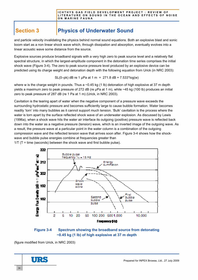
I C H T H Y S G A S F I E L D D E V E L O P M E N T P R O J E C T : R E V I E W O F L I T E R A T U R E O N S O U N D I N T H E O C E A N A N D E F F E C T S O F N O I S E O N M A R I N E F A U N A
Section 3 Physics of Underwater Sound
34
Prepared for INPEX Browse, Ltd., 27 July 2009
and particle velocity invalidating the physics behind normal sound equations. Both an explosive blast and sonic boom start as a non linear shock wave which, through dissipation and absorption, eventually evolves into a linear acoustic wave some distance from the source.
Explosive sources produce broadband signals with a very high zero to peak source level and a relatively flat spectral structure, in which the largest-amplitude component in the detonation time series comprises the initial shock wave (Figure 3-4). The zero to peak source pressure level produced by an explosive device can be predicted using its charge weight and detonation depth with the following equation from Urick (in NRC 2003):
SL(0–pk) dB re 1 µPa at 1 m = 271.8 dB + 7.533*log(w)
where w is the charge weight in pounds. Thus a ~0.45 kg (1 lb) detonation of high explosive at 37 m depth yields a maximum zero to peak pressure of 272 dB (re µPa at 1 m), while ~45 kg (100 lb) produces an initial zero to peak pressure of 287 dB (re 1 Pa at 1 m) (Urick, in NRC 2003).
Cavitation is the tearing apart of water when the negative component of a pressure wave exceeds the surrounding hydrostatic pressure and becomes sufficiently large to cause bubble formation. Water becomes readily ‘torn’ into many bubbles as it cannot support much tension. ‘Bulk’ cavitation is the process where the water is torn apart by the surface reflected shock wave of an underwater explosion. As discussed by Lewis (1996a), when a shock wave hits the water air interface its outgoing (positive) pressure wave is reflected back down into the water as a negative pressure (tension) wave, which is an inverted image of the outgoing wave. As a result, the pressure wave at a particular point in the water column is a combination of the outgoing compression wave and the reflected tension wave that arrives soon after. Figure 3-4 shows how the shock-wave and bubble pulse energies combine at frequencies greater than 1/T (T = time (seconds) between the shock wave and first bubble pulse).
Figure 3-4 Spectrum showing the broadband source from detonating ~0.45 kg (1 lb) of high explosive at 37 m depth
(figure modified from Urick, in NRC 2003)
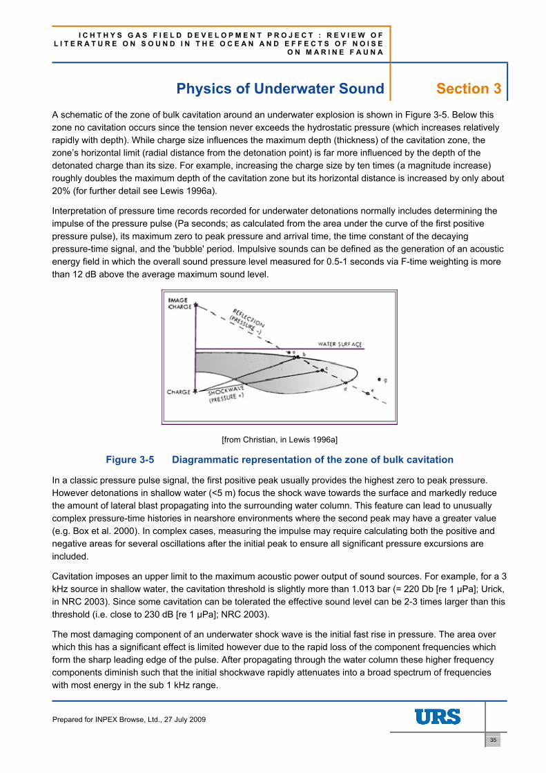
I C H T H Y S G A S F I E L D D E V E L O P M E N T P R O J E C T : R E V I E W O F L I T E R A T U R E O N S O U N D I N T H E O C E A N A N D E F F E C T S O F N O I S E
O N M A R I N E F A U N A
Physics of Underwater Sound Section 3
Prepared for INPEX Browse, Ltd., 27 July 2009
35
A schematic of the zone of bulk cavitation around an underwater explosion is shown in Figure 3-5. Below this zone no cavitation occurs since the tension never exceeds the hydrostatic pressure (which increases relatively rapidly with depth). While charge size influences the maximum depth (thickness) of the cavitation zone, the zone’s horizontal limit (radial distance from the detonation point) is far more influenced by the depth of the detonated charge than its size. For example, increasing the charge size by ten times (a magnitude increase) roughly doubles the maximum depth of the cavitation zone but its horizontal distance is increased by only about 20% (for further detail see Lewis 1996a).
Interpretation of pressure time records recorded for underwater detonations normally includes determining the impulse of the pressure pulse (Pa seconds; as calculated from the area under the curve of the first positive pressure pulse), its maximum zero to peak pressure and arrival time, the time constant of the decaying pressure-time signal, and the 'bubble' period. Impulsive sounds can be defined as the generation of an acoustic energy field in which the overall sound pressure level measured for 0.5-1 seconds via F-time weighting is more than 12 dB above the average maximum sound level.
[from Christian, in Lewis 1996a]
Figure 3-5 Diagrammatic representation of the zone of bulk cavitation
In a classic pressure pulse signal, the first positive peak usually provides the highest zero to peak pressure. However detonations in shallow water (<5 m) focus the shock wave towards the surface and markedly reduce the amount of lateral blast propagating into the surrounding water column. This feature can lead to unusually complex pressure-time histories in nearshore environments where the second peak may have a greater value (e.g. Box et al. 2000). In complex cases, measuring the impulse may require calculating both the positive and negative areas for several oscillations after the initial peak to ensure all significant pressure excursions are included.
Cavitation imposes an upper limit to the maximum acoustic power output of sound sources. For example, for a 3 kHz source in shallow water, the cavitation threshold is slightly more than 1.013 bar (= 220 Db [re 1 µPa]; Urick, in NRC 2003). Since some cavitation can be tolerated the effective sound level can be 2-3 times larger than this threshold (i.e. close to 230 dB [re 1 µPa]; NRC 2003).
The most damaging component of an underwater shock wave is the initial fast rise in pressure. The area over which this has a significant effect is limited however due to the rapid loss of the component frequencies which form the sharp leading edge of the pulse. After propagating through the water column these higher frequency components diminish such that the initial shockwave rapidly attenuates into a broad spectrum of frequencies with most energy in the sub 1 kHz range.

I C H T H Y S G A S F I E L D D E V E L O P M E N T P R O J E C T : R E V I E W O F L I T E R A T U R E O N S O U N D I N T H E O C E A N A N D E F F E C T S O F N O I S E O N M A R I N E F A U N A
Section 3 Physics of Underwater Sound
36
Prepared for INPEX Browse, Ltd., 27 July 2009
3.5 Sound Propagation and Transmission Loss As sound propagates from its source it undergoes transmission loss with increasing distance (range). The most influential processes causing transmission losses in seawater comprise geometric spreading and absorption, which are described in the following subsections.
3.5.1 Geometric spreading As a sound wave radiates from a source, its amplitude and intensity fall as a function of the geometric spreading of its wave front. Wavefronts spread spherically in the near field, and cannot adopt a cylindrical pattern of spreading until attaining a significant distance from the source (typically 100 m or more). Spherical spreading is the propagation of the wavefront in an omni-directional or conical form away from the source. The area of the sound front (mean square pressure) varies inversely with the square of the distance from the source, so sound levels are diminished by 6 dB for every doubling of distance from the source (= 20 dB when distance has increased ten fold). Spherical spreading occurs in the source’s near-field and typically extends for a distance of several times the depth (i.e. the distance required before a sufficient number of ray paths from seafloor reflections produce a ‘wall’ that provides a cylindrical wave front).
Cylindrical spreading develops when the medium is not homogenous, including shallow areas (0-200 m) where the sound waves reflected off a reasonably reflective seafloor as well as from the more mirror-like water surface. The underlying seabed strata can also become part of the media through which the sound propagates, although the propagation efficiency is far less than that of the water column. Cylindrical spreading can be pictured as a widening tin can or fat cylinder, with the wavefront forming the vertical wall. It is never perfect nor commences near a source since it requires sufficient distance (usually several times the water depth) for enough reflections and/or refractions to spread the energy across the entire wavefront.
Since the surface area of a cylinder doubles for every doubling of its radius, the sound front halves for every doubling of the distance from the source. Hence sound levels decrease by 3 dB instead of 6 dB for every doubling of the distance from the source. In practice, cylindrical spreading rarely commences <100 m from the source, with sound transmission losses in both the near- and mid-field best approximated by spherical spreading, particularly for near-surface sources in shelfal waters (e.g. Cato 2003). As an example, Table 3-2 shows how sound levels diminish more slowly with increasing distance if perfect cylindrical spreading commences beyond 64 m from a source (as may occur with a source in water 16 m deep, noting that cylindrical spreading sometimes establishes at distances from source around four times the depth of water).
Cylindrical spreading can occur in deep ocean waters whenever sound waves become ‘trapped’ along an axis (‘duct’) as a result of different temperature and pressure conditions which change their speed and cause alternating bending. The duct is formed by the temperature decline in the upper layer (which reduces the sound speed and thus bends the waves downward, away from the surface), plus the rising water pressure in the deeper layers where temperatures are more uniform (which increases the sound speed and thus refracts the waves upward, away from the seafloor). The depth layer which has the slowest sound speed forms the axis of the duct because of the differing (‘down/up’) wave refractions on either side of it. Mid-water ducts also allow the wavefront to retain energy by preventing the sound waves reaching (and being absorbed by) the seafloor and from reaching (and being scattered by) the surface. Since long waves are more sensitive to the bending effect of sound speed changes, the lower frequency components of a source are more amenable to sound ducting.
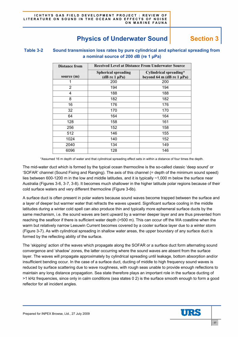
I C H T H Y S G A S F I E L D D E V E L O P M E N T P R O J E C T : R E V I E W O F L I T E R A T U R E O N S O U N D I N T H E O C E A N A N D E F F E C T S O F N O I S E
O N M A R I N E F A U N A
Physics of Underwater Sound Section 3
Prepared for INPEX Browse, Ltd., 27 July 2009
37
Table 3-2 Sound transmission loss rates by pure cylindrical and spherical spreading from a nominal source of 200 dB (re 1 µPa)
Received Level at Distance From Underwater Source Distance from
source (m) Spherical spreading
(dB re 1 μPa) Cylindrical spreading*
beyond 64 m (dB re 1 μPa) 1 200 200 2 194 194 4 188 188 8 182 182 16 176 176 32 170 170 64 164 164
128 158 161 256 152 158 512 146 155 1024 140 152 2040 134 149 6096 128 146
*Assumed 16 m depth of water and that cylindrical spreading effect sets in within a distance of four times the depth.
The mid-water duct which is formed by the typical ocean thermocline is the so-called classic ‘deep sound’ or ‘SOFAR’ channel (Sound Fixing and Ranging). The axis of this channel (= depth of the minimum sound speed) lies between 600-1200 m in the low and middle latitudes, and it is typically ~1,000 m below the surface near Australia (Figures 3-6, 3-7, 3-8). It becomes much shallower in the higher latitude polar regions because of their cold surface waters and very different thermocline (Figure 3-6b).
A surface duct is often present in polar waters because sound waves become trapped between the surface and a layer of deeper but warmer water that refracts the waves upward. Significant surface cooling in the middle latitudes during a winter cold spell can also produce thin and typically more ephemeral surface ducts by the same mechanism, i.e. the sound waves are bent upward by a warmer deeper layer and are thus prevented from reaching the seafloor if there is sufficient water depth (>500 m). This can occur off the WA coastline when the warm but relatively narrow Leeuwin Current becomes covered by a cooler surface layer due to a winter storm (Figure 3-7). As with cylindrical spreading in shallow water areas, the upper boundary of any surface duct is formed by the reflecting ability of the surface.
The ‘skipping’ action of the waves which propagate along the SOFAR or a surface duct form alternating sound convergence and ‘shadow’ zones, the latter occurring where the sound waves are absent from the surface layer. The waves will propagate approximately by cylindrical spreading until leakage, bottom absorption and/or insufficient bending occur. In the case of a surface duct, ducting of middle to high frequency sound waves is reduced by surface scattering due to wave roughness, with rough seas unable to provide enough reflections to maintain any long distance propagation. Sea state therefore plays an important role in the surface ducting of >1 kHz frequencies, since only in calm conditions (sea states 0 2) is the surface smooth enough to form a good reflector for all incident angles.

I C H T H Y S G A S F I E L D D E V E L O P M E N T P R O J E C T : R E V I E W O F L I T E R A T U R E O N S O U N D I N T H E O C E A N A N D E F F E C T S O F N O I S E O N M A R I N E F A U N A
Section 3 Physics of Underwater Sound
38
Prepared for INPEX Browse, Ltd., 27 July 2009
Figure 3-6 Schematic of the mechanism forming the deep sound channel
In summary, both types of geometric spreading are only approximate for most situations, with cylindrical spreading becoming evident whenever wavefronts become (a) refracted by sound speed variations due to changing temperature and pressure, or (b) by sufficient multiple reflections between the surface and an amenable seafloor (i.e. unusually reflective).
Figure 3-7 Simplified schematic showing sound paths from surface and deep sources, and highlighting the transmission and loss process for a surface source (not all paths shown)
(from McCauley et al. 2000)
At both the surface and bottom, sound waves reflect back onto themselves, and these reflections interfere with the original wave to produce an interference pattern in the water column. A single frequency source will produce a discrete number of vertical interference patterns, each with a different number of maximum and minimum pressures from top to bottom. Each vertical interference pattern, or standing wave in the vertical direction, propagates in the horizontal direction at its own speed. However, if the frequency of a standing wave is too low,

I C H T H Y S G A S F I E L D D E V E L O P M E N T P R O J E C T : R E V I E W O F L I T E R A T U R E O N S O U N D I N T H E O C E A N A N D E F F E C T S O F N O I S E
O N M A R I N E F A U N A
Physics of Underwater Sound Section 3
Prepared for INPEX Browse, Ltd., 27 July 2009
39
it will not propagate. This lower frequency limit is called the cut-off frequency, and standing waves with frequencies below the cut-off cannot propagate in the horizontal direction.
A
B
Figure 3-8 Depth profiles showing sound transmission losses in different ocean regimes, as predicted by a parabolic equation model (MMPE) for a low frequency (200 Hz) and
high frequency (3 kHz) source at 50 m depth
(a) shows extended propagation of high frequencies via a shallow surface duct as well as the SOFAR channel (axis of slowest speed is at 1000 m);
(b) shows the shallower location of the sound channel in cool polar waters due to the altered temperature-related sound speed profile.
In summary, the ultimate distance of any sound source’s audible or higher level range is heavily influenced by its depth and frequency characteristics, the water depth and sea surface state, the sound channelling ability of ducts, and the level and type of background noise in the region of the receiver. The complex nature of sound
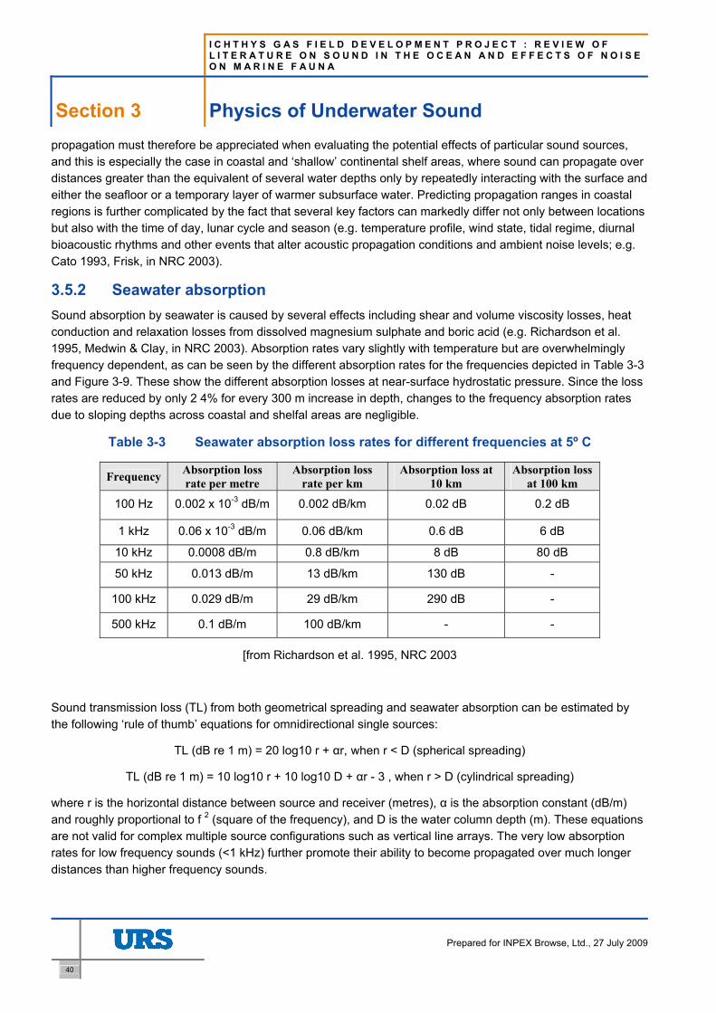
I C H T H Y S G A S F I E L D D E V E L O P M E N T P R O J E C T : R E V I E W O F L I T E R A T U R E O N S O U N D I N T H E O C E A N A N D E F F E C T S O F N O I S E O N M A R I N E F A U N A
Section 3 Physics of Underwater Sound
40
Prepared for INPEX Browse, Ltd., 27 July 2009
propagation must therefore be appreciated when evaluating the potential effects of particular sound sources, and this is especially the case in coastal and ‘shallow’ continental shelf areas, where sound can propagate over distances greater than the equivalent of several water depths only by repeatedly interacting with the surface and either the seafloor or a temporary layer of warmer subsurface water. Predicting propagation ranges in coastal regions is further complicated by the fact that several key factors can markedly differ not only between locations but also with the time of day, lunar cycle and season (e.g. temperature profile, wind state, tidal regime, diurnal bioacoustic rhythms and other events that alter acoustic propagation conditions and ambient noise levels; e.g. Cato 1993, Frisk, in NRC 2003).
3.5.2 Seawater absorption Sound absorption by seawater is caused by several effects including shear and volume viscosity losses, heat conduction and relaxation losses from dissolved magnesium sulphate and boric acid (e.g. Richardson et al. 1995, Medwin & Clay, in NRC 2003). Absorption rates vary slightly with temperature but are overwhelmingly frequency dependent, as can be seen by the different absorption rates for the frequencies depicted in Table 3-3 and Figure 3-9. These show the different absorption losses at near-surface hydrostatic pressure. Since the loss rates are reduced by only 2 4% for every 300 m increase in depth, changes to the frequency absorption rates due to sloping depths across coastal and shelfal areas are negligible.
Table 3-3 Seawater absorption loss rates for different frequencies at 5º C
Frequency Absorption loss rate per metre
Absorption loss rate per km
Absorption loss at 10 km
Absorption loss at 100 km
100 Hz 0.002 x 10⁻³ dB/m 0.002 dB/km 0.02 dB 0.2 dB
1 kHz 0.06 x 10⁻³ dB/m 0.06 dB/km 0.6 dB 6 dB
10 kHz 0.0008 dB/m 0.8 dB/km 8 dB 80 dB
50 kHz 0.013 dB/m 13 dB/km 130 dB -
100 kHz 0.029 dB/m 29 dB/km 290 dB -
500 kHz 0.1 dB/m 100 dB/km - -
[from Richardson et al. 1995, NRC 2003
Sound transmission loss (TL) from both geometrical spreading and seawater absorption can be estimated by the following ‘rule of thumb’ equations for omnidirectional single sources:
TL (dB re 1 m) = 20 log10 r + αr, when r < D (spherical spreading)
TL (dB re 1 m) = 10 log10 r + 10 log10 D + αr - 3 , when r > D (cylindrical spreading)
where r is the horizontal distance between source and receiver (metres), α is the absorption constant (dB/m) and roughly proportional to f 2 (square of the frequency), and D is the water column depth (m). These equations are not valid for complex multiple source configurations such as vertical line arrays. The very low absorption rates for low frequency sounds (<1 kHz) further promote their ability to become propagated over much longer distances than higher frequency sounds.
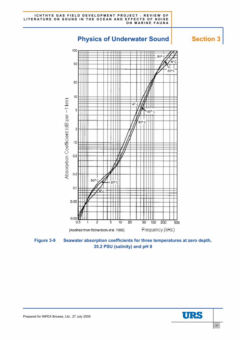
I C H T H Y S G A S F I E L D D E V E L O P M E N T P R O J E C T : R E V I E W O F L I T E R A T U R E O N S O U N D I N T H E O C E A N A N D E F F E C T S O F N O I S E
O N M A R I N E F A U N A
Physics of Underwater Sound Section 3
Prepared for INPEX Browse, Ltd., 27 July 2009
41
Figure 3-9 Seawater absorption coefficients for three temperatures at zero depth, 35.2 PSU (salinity) and pH 8

I C H T H Y S G A S F I E L D D E V E L O P M E N T P R O J E C T : R E V I E W O F L I T E R A T U R E O N S O U N D I N T H E O C E A N A N D E F F E C T S O F N O I S E O N M A R I N E F A U N A
Section 3 Physics of Underwater Sound
42
Prepared for INPEX Browse, Ltd., 27 July 2009
3.5.3 Scattering and other absorption losses Apart from geometric spreading and seawater absorption, transmission losses also occur via:
• surface scattering from wind-generated surface roughness
• bubbles present near the surface as a result of recent wave action
• suspended silts and other particles (turbidity)
• density of sound absorbing phytoplankton and other marine organism tissues (including fish bladders)
• seabed topography, sediment type and thickness (seabed absorption is typically 1000 or more times that of seawater, and can be 100% depending on the frequencies of interest)
• scattering and leakage at boundaries between water masses with different temperature, salinity and/or turbidity properties
• Intervening landmasses, including reefs, shoals and mudflats.
Accurate prediction of sound transmission loss rates is therefore a complex function involving the environmental parameters of the water column as well as the source and receiver depth-range geometry, source spectrum, sea surface conditions and the proximity, contours and type of the seabed (e.g. Richardson et al. 1995, Gisiner 1998, McCauley & Cato 2003, NRC 2003).
3.5.4 Propagation modelling and transmission anomalies Propagation models utilise bathymetric databases, geo-acoustic information, oceanographic parameters and boundary roughness models in attempts to estimate the acoustic field at points far from a sound’s source in the face of various unknowns that cause transmission anomalies. The quality of these estimates is related to the choice of model and the quality and quantity of the available environmental information. In continental shelf waters where transmission anomalies may include a number of significant geoacoustic effects such as compressional sound speeds, bottom topographic roughness and sediment density, sound pathways can be readily altered and estimates of propagation loss can be out by ±10 dB or more.
In the case of transient sounds, the properties of sound pulses received at >20 km from their source can be quite different from the signal emitted by the source, particularly if they have propagated across shallow coastal waters before reaching a receiver located in deeper offshore waters. In the case of airgun arrays, for example, duration of received pulses is often increased by a factor of 20-40, while the centre frequency emphasis can climb from ~50 Hz to between 110-260 Hz (e.g. McCauley et al. 1998, 2000, Madsen et al. 2003). This shift is characteristic of shallow water propagation in which the signals become high-pass filtered (Richardson et al. 1995).
These changes reflect the effects of multipath propagations involving multiple surface/bottom reflections, and where the contents of the received signal contain the sum of wave energies arriving from different transmission pathways. Their slightly different arrival times at the receiver produce ‘smeared out’ waveforms, with the duration of the ‘chirp’ like signal that contains audible energies (~10 dB above background) lasting for one second or more (e.g. Greene & Richardson 1988, Bowles et al. 1994, Madsen et al 2003).

I C H T H Y S G A S F I E L D D E V E L O P M E N T P R O J E C T : R E V I E W O F L I T E R A T U R E O N S O U N D I N T H E O C E A N A N D E F F E C T S O F N O I S E
O N M A R I N E F A U N A
Physics of Underwater Sound Section 3
Prepared for INPEX Browse, Ltd., 27 July 2009
43
In summary, predicting sound transmission losses for a particular source at a particular location and time depends heavily on the type and quality of available environmental data and empirical evidence, since the propagation can involve multiple pathways that are influenced by:
• the frequency energy spectrum, waveform and depth of the sound source
• velocity/rise time and duration of the source signal (for impulses)
• uniformity of the water depth (seafloor bathymetry)
• sea surface state
• water temperature, salinity and turbidity profile (especially the presence and depth of any disjunct thermal or salinity boundaries in the water column)
• variations in the geoacoustic properties of the seabed along the direction/s of interest, including the seafloor topography, rugosity and strata composition and thickness
• the proximity and complexity of surrounding or intervening land.
There are four main types of propagation models used in underwater acoustics:
• Parabolic equation (PE).
• Normal mode.
• Wave number integration.
• Ray code models.
Each group provides a different approach to simplifying either the acoustic wave equation (containing the basic physics of sound propagation), the influence of the environment or both. The performance of each type depends on the range and sound frequencies being modelled and the environmental characteristics. In general, PE models perform well for range dependent environments for frequencies below 1 kHz, although normal mode models can be more efficient and accurate for modelling these frequencies in strongly range-dependent environments. Ray code models are usually efficient for frequencies above 1 kHz in many environments.


I C H T H Y S G A S F I E L D D E V E L O P M E N T P R O J E C T : R E V I E W O F L I T E R A T U R E O N S O U N D I N T H E O C E A N A N D E F F E C T S O F N O I S E
O N M A R I N E F A U N A
Ambient Noise in the Ocean Section 4
Prepared for INPEX Browse, Ltd., 27 July 2009
45
4 Ambient Noise in the Ocean
This section describes the characteristics of ambient noise in the ocean and the natural components of that noise to identify the range of noise levels to which marine fauna are naturally exposed. Natural sources are described in more detail in Section 5 and anthropogenic sources in Section 6.
Ambient noise refers to the overall background noise from both natural and human sources such that the contribution of a specific source is not readily identifiable. The term ‘ocean noise’ has been used by the National Research Council (NRC 2003) to encompass not only background noise but also sounds from distinguishable nearby sources such as individual ships or pods of whales.
Ambient noise levels are generally reported as ranges of sound pressure level recorded over various sampling periods. Any consideration of ambient noise levels needs to recognise that the indicated levels are actually averages over the selected sampling period. The averaging period used influences the indicated noise level. Short period, transient natural events can produce noise spikes far in excess of the assigned average level for any particular natural phenomenon.
The primary sources of mid-ocean ambient noise are weather effects, tectonic activity, ocean wave interactions (‘microseisms’) thermal agitation and distant shipping traffic (Figures 4-1 and 4-2). Examples of the differences in ambient noise levels, make-up and energy spectra, including deep sea versus coastal waters and regional differences are given in Urick (1983) and Cato (2000). The ambient noise level and frequency spectrum can be predicted for most deep-water areas from known shipping traffic density and the wind speed, Beaufort force or sea state. Heavy rainfall can cause significant but localised increases (Section 5.2.4), since this surface source has significant vertical directionality (to 45º) and therefore less range than omnidirectional and horizontal near-surface sources (e.g. Cato 2000).
Broadband ambient noise spectrum levels 7 range from 45-60 dB in quiet regions (light shipping and calm seas) to 80-100 dB for more typical conditions and over 120 dB (re 1 μPa) 8 during periods of high winds, rain or biological choruses. In the 100-500 Hz range, Urick (1983) estimated average deep water ambient noise spectra of 73-80 dB for areas of heavy shipping traffic and relatively high sea states and 46-58 dB for areas with light shipping and calms.
Background levels in the 20-500 Hz range are frequently dominated by distant shipping, particularly in heavy traffic regions. Vocalisations of the great whales also contribute to this low frequency band, with the duration and frequency of these choruses increasing in breeding, migrating and feeding areas as stocks recover from past whaling (Croll et al. 2001, McCauley & Cato 2003). Above 300-400 Hz the level of weather-related sounds exceeds shipping noise, with wind wave conditions and nearby rainfall dominating the 500-50,000 Hz range.
7 The level of a sound wave in a 1 Hz wide frequency band (Urick 1983; see also Figure 4-1). Reported spectrum levels are assumed to reflect mean square pressure unless otherwise stated.
8 Measure of underwater noise, in terms of sound pressure. As noted previously, the dB is a relative measure, rather than an absolute measure; it must be referenced to a standard “reference intensity”, in this case 1 micro Pascal (1μPa), which is the standard reference that is used. The dB is also measured over a specified frequency, which is usually either a one Hertz bandwidth (expressed as dB (re 1μPa2/Hz), or over a broadband which has not been filtered. Where a frequency is not specified, it can be assumed that the measurement is a broadband measurement.

I C H T H Y S G A S F I E L D D E V E L O P M E N T P R O J E C T : R E V I E W O F L I T E R A T U R E O N S O U N D I N T H E O C E A N A N D E F F E C T S O F N O I S E O N M A R I N E F A U N A
Section 4 Ambient Noise in the Ocean
46
Prepared for INPEX Browse, Ltd., 27 July 2009
Figure 4-1 Generalised ambient noise spectra attributable to various sources
(compiled by Wenz 1962; reproduced from Richardson et al. 1995)

I C H T H Y S G A S F I E L D D E V E L O P M E N T P R O J E C T : R E V I E W O F L I T E R A T U R E O N S O U N D I N T H E O C E A N A N D E F F E C T S O F N O I S E
O N M A R I N E F A U N A
Ambient Noise in the Ocean Section 4
Prepared for INPEX Browse, Ltd., 27 July 2009
47
Figure 4-2 Pressure density curves of ambient noise components
Top: Australian waters (Cato 1995)
Bottom: From Defence Science and Technology Organisation (DSTO) survey site off Perth
In contrast to deep sea regions, ambient noise levels and frequency components across shelfal and nearshore waters are far more variable with season, location and time of day and are less amenable to prediction without local measurements. While the key sources remain shipping and local weather patterns, contributions from marine biota as well as various fishing, boating and industrial noises near ports, Harbours and marinas become significant, with the level and composition changing with time and place (Cato 2000; Urick 1983).

I C H T H Y S G A S F I E L D D E V E L O P M E N T P R O J E C T : R E V I E W O F L I T E R A T U R E O N S O U N D I N T H E O C E A N A N D E F F E C T S O F N O I S E O N M A R I N E F A U N A
Section 4 Ambient Noise in the Ocean
48
Prepared for INPEX Browse, Ltd., 27 July 2009
In regions with feeding or breeding great whales, whale vocalisations vary by season, week, day and hour and can boost background noise levels to over 120 dB (re 1 μPa) (e.g. 110-136 Db [re 1 μPa [rms]] at ⅓OB 300 Hz, with 123 dB [re 1μPa] peaks at 315 Hz 9), as measured in March and April 1998 at four locations off Maui where humpback whales were not in the vicinity of the receivers (Au & Green 2000). The type, intensity and propagation of sources contributing to ambient noise in coastal waters are also more spatially variable as a consequence of finer scale changes in seafloor topography and seafloor substrate. Levels increase where more reflective rocky substrates are prevalent and decrease where thick absorptive layers of fine sediments and mud occur.
Turbulence and seafloor saltation noise induced by strong tidal streams can also become locally dominant, particularly in coastal parts of northern Australia with large tidal ranges, and where noise levels fluctuate widely according to local tidal flow rates and bottom types. Ambient noise in Kimberley embayments that contain coarse gravely sediments can exceed 110-120 dB on a diurnal basis, particularly during spring ebb and flood tides (URS 2008).
Published plots of low and high frequency ambient noise indicate that the waters surrounding Australia (Figure 4-2) are similar to those elsewhere except for the noisier areas of busy shipping traffic in south Asia, east Asia and NW Atlantic-European waters (see e.g. the colour global sound charts in NRC 2003).
9 When evaluating the literature it is important to check the measure used when interpreting reported pulse levels. Geophysical studies frequently record peak-to-peak values (dB (re 1 μPa at 1 m)), while the ‘peak level’ (zero to peak) for the same pulse is typically some 6 dB less. Received sound levels of airgun pulses in biological reports are often given as the average level (root mean square; rms), which represents the mean sound pressure level over the duration of the pulse. These are typically some 10 dB lower than the zero-peak level of airgun pulses and often 16 dB lower than the peak-peak value (e.g. Greene 1997, McCauley et al. 1998, 2000a). The energy level (dB (re 1 μPa2 per second) is less frequently used and is always lower than rms pressure level because the pulses are less than 1 second.

I C H T H Y S G A S F I E L D D E V E L O P M E N T P R O J E C T : R E V I E W O F L I T E R A T U R E O N S O U N D I N T H E O C E A N A N D E F F E C T S O F N O I S E
O N M A R I N E F A U N A
Natural Sources of Noise in the Ocean Section 5
Prepared for INPEX Browse, Ltd., 27 July 2009
49
5 Natural Sources of Noise in the Ocean
5.1 Characteristics of Natural Ambient Noise The following sections describe the naturally sourced sounds that contribute to the ambient background of ocean noise. In the absence of shipping, natural sources are the dominant sources of the long-term time-averaged ocean noise at all frequencies, including whale calling in many regions (e.g. McCauley & Cato 2003). Even in the presence of distant shipping, contributions from a range of natural sources dominate the ocean noise spectra below 5 Hz and from a few 100 Hz to 200 kHz.
The dominant source of natural noise across the 1-100,000 Hz range is associated with sea surface waves generated by wind acting on the sea surface. Non-linear interactions between ocean surface waves, previously called ‘microseisms’, are the dominant contributors below 500 Hz (referred to as ‘Surface Waves Second-Order Pressure Effects’ in the classical Wenz curves of ambient noise). The dominant contributor above 50,000 Hz is thermal noise, which arises from pressure fluctuations associated with the molecular agitation of the ocean medium itself (Section 5.2.5).
Natural biological sound sources make significant contributions in certain regions, seasons and times of day. For example the natural noise from snapping shrimps (from ~5 kHz to 300 kHz) forms an important component close to reefs and in rocky bottom regions in shallow waters in <40º latitudes, reaching crescendo proportions in <60 m deep areas near tropical coasts. Fish choruses can significantly add to ocean noise in many locales, while groups of whistling and echo-locating dolphins can raise local noise levels in the frequency range of their signals. An almost infrasonic peak around 20 Hz created by modulation of the calls of large baleen whales, often referred to as ‘whale ticks’ (e.g. Au & Green 2000), is often present in deep-ocean spectra, while choruses of humpback whales reach broad peaks near 300 Hz,. Around Australia, the Timor/Arafura Sea region has the most divergent ambient noise signature owing to the dominant role of biological sources plus distinctive fish sounds (Cato 2000).
5.2 Components of Natural Ambient Noise The frequency ranges of the following common natural physical and biological sources of relatively intense, persistent and/or frequent noise are shown in Figures 5-1 and 5-2, with their source levels listed in Table 5-1.
Physical: Subterranean vents, tremors, earthquakes, eruptions, sediment slumps and other tectonic activity; lightning strikes, microseisms; thermal noise, ice cracking, wind waves, surf, rainfall, tidal turbulence and seafloor saltation.
Biological: Sea urchins, snapping shrimp, Sciaenid croakers (jewfish, mulloway, etc), other fish choruses, high frequency whistles and echolocation clicks (dolphins and other toothed whales), low frequency vocalisations (great whales, including near-infrasonic calls from rorqual species), unidentified ‘biotics’.

I C H T H Y S G A S F I E L D D E V E L O P M E N T P R O J E C T : R E V I E W O F L I T E R A T U R E O N S O U N D I N T H E O C E A N A N D E F F E C T S O F N O I S E O N M A R I N E F A U N A
Section 5 Natural Sources of Noise in the Ocean
50
Prepared for INPEX Browse, Ltd., 27 July 2009
Table 5-1 Examples of intense natural sound sources
Source Type Location and Timing
Perceived Direction Periodicity Frequency
range (Hz) Source Level*
Tectonic quakes, tremors, eruptions Unpredictable Seafloor or
circumferential Sudden irregular transients
(2-20 mins) LF (10-100) 220-250
Lightning Unpredictable Surface Sudden short pulse Broadband ~260 Breaching and fluke slapping Variable Surface Sudden pulse Broadband 170-190
Baleen whale songs and moans Variable Variable Variable continuous or
transients LF-MF + harmonics 170-195
Delphinid whistles and squeals Variable Variable Mostly anticipated
transients HF-VHF
(>10 kHz) 180-195
Sperm whale click, codas and creaks Variable Variable Mostly anticipated
transients HF 180-235
Toothed whale echolocation sonar Variable Variable Mostly anticipated
pulses or click bursts HF-VHF
(>10 kHz) 190-232
Sea ice noises Surface Multiple surface points Variable transients Broadband 120-190
Rough weather and rain Surface Background Irregular, continuous Broadband 80-120*
Tide turbulence and saltation Seafloor Background Regular, continuous Broadband 80-120*
Fish choruses Variable Stationary / background Regular continuous
LF and MF/HF tonals
80-120*
Snapping shrimps Seafloor Stationary / background Regular, continuous LF-MF 80-120*
* dB (re µP at 1 m) peak-peak
(from University of Rhode Island [undated], NOAA 2002, Cato 2000, Simon et al. 2003.)
5.2.1 Eruptions, tremors and other tectonic events Seismic events from tectonic activity produce one of the most intense sources of natural noise. Undersea earthquakes, seafloor venting and volcanic activity frequently provide sources of intense low frequency sound. Sounds from volcanic eruptions and resonance tremors in the Pacific Ocean are routinely detected and recorded across distances of thousands of miles.
Fox et al. (2002) noted that seismic monitoring since 1991 shows that natural seismic activity in the Pacific Basin produces nearly 10,000 acoustic events annually that involve source levels >200 dB (re 1 μPa 1m). Arriving signals often have sudden, sharp onsets and can last from several seconds to several minutes, with frequencies extending from the infrasonic to over 100 Hz.
Earthquakes produce a triangular-shaped acoustic energy signal known as ‘T-waves’. The T-phase duration is related to the earthquake magnitude, and these produce the highest acoustic energy in the 5-35 Hz frequency range (e.g. Nishimura & Clark 2001). A T-wave showing the highest acoustic energy in the 5-30 Hz range is shown in Figure 5-1 (the yellows and reds).

I C H T H Y S G A S F I E L D D E V E L O P M E N T P R O J E C T : R E V I E W O F L I T E R A T U R E O N S O U N D I N T H E O C E A N A N D E F F E C T S O F N O I S E
O N M A R I N E F A U N A
Natural Sources of Noise in the Ocean Section 5
Prepared for INPEX Browse, Ltd., 27 July 2009
51
Figure 5-1 Triangular shaped low frequency signal from subsea earthquake
Plots of T-waves recorded by both SOSUS 10 and NOAA’s Eastern Equatorial Pacific autonomous hydrophone array 11 during the February 1996 Gorda eruption (near 42º40'N and 126º48'W in the northeast Pacific), and the
10 The SOund SUrveillance System (SOSUS) is a fixed component of the US Navy's Integrated Undersea Surveillance Systems (IUSS) network that was deployed for deep ocean surveillance during the Cold War. Installation of SOSUS began in the mid 1950s for use in antisubmarine warfare SOSUS consists of bottom mounted hydrophone arrays connected by undersea communication cables to facilities on shore. The individual arrays are installed primarily on continental slopes and seamounts at optimal locations for receiving undistorted long range acoustic propagation. The combination of location within the oceanic sound channel and the sensitivity of large-aperture arrays allows the system to detect radiated acoustic power of less than one watt at ranges of several hundred kilometres. A brief history of SOSUS and its current use is at http://www.globalsecurity.org/intell/systems/sosus.htm.
11 In October 1990, NOAA was permitted to access the SOSUS arrays in the North Pacific for ocean environmental monitoring. The data collection systems developed by NOAA's VENTS Program were implemented in August 1991, with acoustic signals from the north Pacific Ocean recorded at NOAA’s Pacific Marine Environmental Laboratory (PMEL) in Newport, Oregon. PMEL has subsequently deployed moored autonomous hydrophones for monitoring remote ocean areas not covered by fixed arrays such as SOSUS. PMEL is the primary centre for both continuous monitoring of low-level seismicity around the northeast Pacific Ocean and real-time detection of intense volcanic activity along the northeast Pacific spreading centres, in support of NOAA’s VENTS research on ocean hydrothermal systems. Its first array was deployed in the eastern equatorial Pacific in May 1996 to long-term monitor the East Pacific Rise between 20N-20S. Other arrays have since been deployed on the centre ridge of the Atlantic Ocean. Real-time ridge crest monitoring permits timely on-site investigations of hydrothermal and magma emissions. Hydrophones have also been deployed in the Gulf of Alaska for marine mammal monitoring in 2000. The sensitive PMEL arrays have recorded several airgun sources from around the Atlantic Basin, sometimes simultaneously. The most frequent originating locations are near Nova Scotia (Canada), northeast Brazil and northwest Africa. Airgun signals have occurred in approximately 75% of the annual data recordings of the Atlantic arrays. More information is at http://www.pmel.noaa.gov/vents/acoustics/haru_system.html.

I C H T H Y S G A S F I E L D D E V E L O P M E N T P R O J E C T : R E V I E W O F L I T E R A T U R E O N S O U N D I N T H E O C E A N A N D E F F E C T S O F N O I S E O N M A R I N E F A U N A
Section 5 Natural Sources of Noise in the Ocean
52
Prepared for INPEX Browse, Ltd., 27 July 2009
1993 lateral magma injection and subsequent eruption at the ‘CoAxial Segment’ site (on the Juan de Fuca Ridge at 46°30'N) are shown in Figure 5-2(a,b). The latter event comprised a dike injection and eruption episode during June-July 1993, and intense T-waves were generated during the latter part of this event. The flow site was subsequently investigated by Canada’s remotely operated vehicle ROPOS in mid-July 1993, where it found and mapped a fresh venting lava flow 2.5 km long plus extensive venting along a nearby 4 km tract.
Figure 5-2 Colour spectrograms showing examples of T-waves
a) Recorded during the 1996 Gorda eruption
b) Recorded during the 1993 Coaxial segment magma injection
[one minute ticks along the x-axis, 0-75 Hertz along the y-axis; from PMEL (2006)].
The seismicity of the Gorda and Coaxial segment events are very similar, in which a rapid series of earthquakes occurs without large ‘foreshocks’ (Figure 5-2(a,b)). The histogram in Figure 5-3 shows the number of events recorded per hour for each event. The apparent decline in activity of the Gorda seismic events from midday day 62 to late day 65 was probably due to loss of the closest array.
The various hydrophone arrays in the Pacific and Atlantic Oceans have been monitoring these types of seismic events for many years. A long-lasting example comprises the extremely loud tremor-like signals which emanated from the volcanically active island chain south of Japan. This is the so-called ‘Inferred Harmonic Tremor’ which developed on 30 separate occasions between May 1998 and December 1999 (PMEL 2006). The precise source was beyond the optimal array coverage but the best estimates place it

I C H T H Y S G A S F I E L D D E V E L O P M E N T P R O J E C T : R E V I E W O F L I T E R A T U R E O N S O U N D I N T H E O C E A N A N D E F F E C T S O F N O I S E
O N M A R I N E F A U N A
Natural Sources of Noise in the Ocean Section 5
Prepared for INPEX Browse, Ltd., 27 July 2009
53
between 22-27ºN and 138-141ºE. The signals were characterized by a high amplitude fundamental at ~10 Hz plus three harmonics at 20, 30, and 40 Hz. The signals typically appeared as discrete packets lasting 4-5 minutes, with brief quiescent periods of roughly 30 seconds followed by the beginning of the next packet of signals (Figure 5-4). During each signal packet, the spectral peaks typically rose by 5-10 Hz while maintaining their harmonic spacing. The largest peak amplitudes and longest durations occurred on four separate occasions during August 1998, on seven widely spaced occasions during 1999 and continued into 2000. The distinctive spectral characteristics have been previously seen in volcanic tremor signals recorded by seismic and airborne equipment from the Arenal and Pavlof volcanos in Costa Rica and Alaska (PMEL 2006).
Figure 5-3 Frequency of events during the Gorda (top) and Coaxial segment (bottom) episodes
[from PMEL (2006)].

I C H T H Y S G A S F I E L D D E V E L O P M E N T P R O J E C T : R E V I E W O F L I T E R A T U R E O N S O U N D I N T H E O C E A N A N D E F F E C T S O F N O I S E O N M A R I N E F A U N A
Section 5 Natural Sources of Noise in the Ocean
54
Prepared for INPEX Browse, Ltd., 27 July 2009
Figure 5-4 A 900 second (15 minute) portion of the 'Inferred Harmonic Tremor' that was detected south of Japan on many separate occasions in 1998-2000.
[from PMEL (2006)]
Figure 5-5 shows a 10 minute (600 second) spectrogram from the SOund SUrveillance System (SOSUS) autonomous deep water hydrophones in the western North Atlantic. The green-highlight shows a low frequency T-wave from an earthquake event in the mid-Atlantic, while the blue- and pink highlighted dark vertical streaks are vocalisations of humpback and minke whales in the vicinity of the array. The spectrogram and sound file show the earthquake produced a loud, low frequency rumble. This recording is on the Office of Marine Programs (OMP) sounds page as an example of how typical tectonic events do not apparently cause marked responses to baleen whale calling behaviour. Such statements would benefit from a longer spectrogram (i.e. showing the type and periodicity of calls recorded for at least the same period before the event of interest as that made after it). It is also unclear if the humpback auditory range is as sensitive to low frequency sounds as those considered likely for the minke and larger rorquals (i.e. the blue and fin whales).
Figure 5-5 600 second (10 minute) spectrogram showing whale calls recorded by the West Atlantic SOSUS array during and after a subsea earthquake
(from OMP 2006)
The northern waters of Australia are occasionally exposed to the intense low frequency sounds which emanate from major tectonic events along the Indonesian-Melanesian island chain, some of which also produce tidal

I C H T H Y S G A S F I E L D D E V E L O P M E N T P R O J E C T : R E V I E W O F L I T E R A T U R E O N S O U N D I N T H E O C E A N A N D E F F E C T S O F N O I S E
O N M A R I N E F A U N A
Natural Sources of Noise in the Ocean Section 5
Prepared for INPEX Browse, Ltd., 27 July 2009
55
waves that reach northwest Australian shorelines. Australian waters are not immune to local natural seismic sources, since smaller earthquakes (magnitude 4 or less) are not uncommon. On average 17 moderate sized earthquakes occur annually on Australia’s continental shelf, while seven seismic events were recorded in 21 days in the deep sound channel off Cape Leeuwin (southwest Australia) in June-July 1998 (Pidcock et al. 2003).
5.2.2 Ocean-wave interactions (microseisms) ‘Microseisms’ are the dominant below 10 Hz natural noise source in the space and time averaged ocean noise spectra (Section 6-1). This source is generated by non-linear interactions of ocean surface waves. Oppositely propagating waves produce a standing wave pattern that radiates sound with twice the frequency of that of the interacting surface waves. These waves are not related to tectonic processes but were termed ‘microseisms’ by seismologists because they are also the dominant source of noise in high quality, on-land seismometer measurements. The Wenz-Curves include ‘Seismic Background’ (Figure 4-1) but it is now known that earthquakes and other tectonic processes contribute only intermittently while the ocean wave interactions provide an almost continuous source of ocean noise in the low frequency range.
5.2.3 Lightning strikes Underwater recordings of spectra of a received sound of thunder from a storm 5-10 km away show a peak between 50 and 250 Hz up to 15 dB above background levels, with detectable energy down to 10 Hz and up to 1 kHz (Dubrovsky & Kosterin 1993, in NRC 2003; Hill 1985). Lightning strikes produce one of the loudest natural sounds in the ocean, generating low tonal impulses with source levels close to the ocean surface of about 260 dB (re 1 μPa at 1 m) (Arnold, Bass & Atchley 1984; Hill 1985; OMP 2006). Analysis of underwater records indicates the sound has an inherent ability for substantial propagation as most of the energy is in the 10-1000 Hz range, with peaks between 100-300 Hz (Figure 5-6). Most lightning activity is recorded during thunderstorms which have lifetimes usually less than an hour and with fronts as small as 5-10 km. Sometimes thunderstorms are arranged in lines hundreds of kilometres long or form large circular clusters.

I C H T H Y S G A S F I E L D D E V E L O P M E N T P R O J E C T : R E V I E W O F L I T E R A T U R E O N S O U N D I N T H E O C E A N A N D E F F E C T S O F N O I S E O N M A R I N E F A U N A
Section 5 Natural Sources of Noise in the Ocean
56
Prepared for INPEX Browse, Ltd., 27 July 2009
Figure 5-6 Spectrogram of an underwater recording of a lightning strike
[recording from the DFO Institute of Ocean Sciences, British Columbia, Canada]
As shown in Figure 5-7, lightning activity is generally less over the oceans than land. The broader Darwin region receives approximately 6-8 ground flashes per km² per year (see Figure 5-8). Darwin Harbour covers an area of approximately 500 km2, and as such from these figures it can estimated that this area may potentially experience between 3000 and 4000 lightning ground flashes per year.

I C H T H Y S G A S F I E L D D E V E L O P M E N T P R O J E C T : R E V I E W O F L I T E R A T U R E O N S O U N D I N T H E O C E A N A N D E F F E C T S O F N O I S E
O N M A R I N E F A U N A
Natural Sources of Noise in the Ocean Section 5
Prepared for INPEX Browse, Ltd., 27 July 2009
57
Figure 5-7 Global distribution of lightning flash density (km2) per annum
[from http://thunder.msfc.nasa.gov/otd/images/global_ltg_from_paper.JPG ]
Figure 5-8 Australian annual lightning ground flash density
[from http://www.bom.gov.au/cgi-bin/climate/cgi_bin_scripts/thunder-light.cgi]

I C H T H Y S G A S F I E L D D E V E L O P M E N T P R O J E C T : R E V I E W O F L I T E R A T U R E O N S O U N D I N T H E O C E A N A N D E F F E C T S O F N O I S E O N M A R I N E F A U N A
Section 5 Natural Sources of Noise in the Ocean
58
Prepared for INPEX Browse, Ltd., 27 July 2009
5.2.4 Wind and rain sources Wind is almost omni-present and its acoustic signature is discernible most of the time (e.g. Richardson et al. 1995, Quartly 2002). Wind generates subsurface sound via the production of breaking waves and generation of subsurface bubbles, with a frequency range from 200 to 50,000 Hz. Although the production of bubbles appears to visibly commence once wind speeds exceed ~5 ms-1 and breaking waves form 'white caps’, bubbles are produced even under very light winds (Quartly 2002). The movement and breaking of these bubbles cause strong underwater sounds. The typical noise spectra due to wind-induced wave and bubble formation increase with wind speed and fall off with frequency (Figure 5-9(a)).
Figure 5-9 Underwater spectrograms
(a) different wind speeds (in m s-1) and (b) rainfall, and (c) rainfall rate probability distributions when raining. (c) upper panel = Nov-Dec 1999; (c) lower panel = May-Jun 2000
[All data for Loch Etive in Scotland, reproduced from Quartly 2002.]
Recent meteorological events and shipping activity can have an effect, as both strong winds and heavy rain produce a sub-surface bubble layer that takes time to dissipate and attenuates the higher frequencies generated by any subsequent surface sources (Quartly 2002). Bubbles left in the wake of passing ships can be identified for almost an hour after the event. Heavy swells produced by storms many hundreds or thousands of kilometres away can arrive on exposed beaches to produce large plunging breakers which can raise local ambient levels over 20 dB for up to 1 km offshore from big surf beaches.
Rain produces a loud, distinctive signal that can increase ambient noise by up to 35 dB across a wide band (100 Hz-50 kHz; Figures 4-1, 4-2). Drizzle produces a characteristic ~14 kHz peak while the intensity of the frequency spectra of heavy rain often exceed that of wind (Figure 5-9(b,c)). Rain generates sound in several ways including the direct impact of droplets, although the bubbles produced by air entrainment during the splashes are the noisiest component. For most raindrop sizes and angles, the bubble sounds provide the loudest component. Small raindrops (0.8-1.2 mm) generate frequencies between 10-25 kHz. Medium raindrops (1.2-2.0 mm) are quiet due to poor air entrainment while large (2.0-3.5 mm) and very large (>3.5 mm) raindrops trap large bubbles which generate frequencies as low as 1 kHz. Sound recordings of rainfall can be used to measure rainfall rate, raindrop size and other features, and are helping meteorologists, oceanographers and climatologists in climate change studies.
Because different raindrop sizes produce distinctive sounds, the underwater sound can be inverted to quantitatively measure drop size distribution in the rain. Acoustical Rain Gauges (ARGs) are being deployed on

I C H T H Y S G A S F I E L D D E V E L O P M E N T P R O J E C T : R E V I E W O F L I T E R A T U R E O N S O U N D I N T H E O C E A N A N D E F F E C T S O F N O I S E
O N M A R I N E F A U N A
Natural Sources of Noise in the Ocean Section 5
Prepared for INPEX Browse, Ltd., 27 July 2009
59
oceanic moorings to make long-term measurements of rainfall using this acoustical technique (for details see Applied Physics Laboratory, University of Washington; http://students.washington.edu/binbing/publication.html ).
Darwin has a mean annual rainfall of 1711 mm, with rain falling on an average of 111 days, mainly in the wet season. A range of monthly rainfall averages received at Darwin Airport (highest, mean and lowest monthly rainfall) is presented in Figure 5-10 (BOM 2008b).
During the wet season Darwin is dominated by westerly and west-north-west winds. Dry season winds vary from the southeast through to the north. The monsoonal tropics also experience cyclone activity. The strongest winds and heaviest rainfall are associated with the passage of tropical cyclones, which can occur in the region at any time during the period November to April.
Figure 5-10 Average monthly rainfall for Darwin (mm)
5.2.5 Thermal noise Thermal noise is generated by pressure fluctuations associated with the thermal molecular agitation of the ocean medium itself. It is what remains when all other noise sources are removed and so provides the lowest bound for noise levels in the ocean. Depending on sea state, thermal noise dictates the shape and level of ambient noise spectra above 50 kHz (Figures 4-1, 2-2; NRC 2003).
5.2.6 Biological sources Before focusing on cetaceans, it is worth noting the sound levels and frequency ranges of some of the noises produced by other marine biota. These noises are dominated by sizzling and crackling sound of snapping shrimps, the croaks, grinding and grunting sounds of croaker fishes and fish choruses, which generate major peaks in the frequency ranges shown in Figures 4-1 and 4-2. The teeth-grinding action of sea urchins resonates through their body shell and forms another significant biological sound in reef areas. Snapping shrimp are a dominant evening source in many sub-tropical and tropical shelfal waters, while loud fish choruses are common

I C H T H Y S G A S F I E L D D E V E L O P M E N T P R O J E C T : R E V I E W O F L I T E R A T U R E O N S O U N D I N T H E O C E A N A N D E F F E C T S O F N O I S E O N M A R I N E F A U N A
Section 5 Natural Sources of Noise in the Ocean
60
Prepared for INPEX Browse, Ltd., 27 July 2009
around Australia’s coasts, particularly after sunset and near dawn (Figure 4-2; see Cato 2000 for more details). Turtles do not vocalise (Richardson et al. 1995).
Whales, dolphins and porpoises produce a wide range of sound covering the frequencies between 10 and 20,000 Hz, and there are many web sites containing spectrograms and sound files of recorded vocalisations 12 covering a range of species. Some of these sites also provide audio file examples of various unidentified ‘bloops’ ‘slow-downs’ and other presumed biological sounds (some possibly cetacean) whose source is unknown.
The dolphins and other toothed species (Odontocetes) typically produce all of the higher frequency (>5000 Hz) calls, whistles and echolocation pulses (with the exception of the songs of male humpback whales), while the baleen whales (Mysticetes) vocalise in the low to mid range, with the larger rorquals producing low to very low (infrasonic) frequencies (Figure 5-11).
It is not exactly understood how the various types of call and echolocation pulses are generated, although the melon is known to be critical for focusing the typically intense echolocation pulses and clicks in the Odontocetes. Estimates of the source level of the 38 microsecond broadband clicks produced by orcas when searching and feeding on Norwegian herring are in the 187-213 dB (re 1µ Pa [peak-peak] 1 m) range, with centre frequencies of 26-57 kHz; (Simon et al. 2003). These frequencies lie in the highest sensitivity zone of the orca audiogram. By contrast, an underwater tail slap used by orcas to stun herring produces a broadband multi pulsed sound with an estimated source level of 187 dB (re 1µPa [peak-peak] at 1 m) (Simon et al. 2003).
12 The term ‘vocalisation’ refers to any sound intentionally produced by a marine mammal that may be used for communication, orientation, prey detection, feeding or breeding. It does not imply that marine mammals use vocal folds, i.e. by exhaling lung air to vibrate vocal cords in base of the throat.

I C H T H Y S G A S F I E L D D E V E L O P M E N T P R O J E C T : R E V I E W O F L I T E R A T U R E O N S O U N D I N T H E O C E A N A N D E F F E C T S O F N O I S E
O N M A R I N E F A U N A
Natural Sources of Noise in the Ocean Section 5
Prepared for INPEX Browse, Ltd., 27 July 2009
61
Figure 5-11 Frequency range for some baleen whales and dolphins
(Keyboard shows fundamental musical scale; adapted from McCauley [2003])
The following subsections describe the vocalisations of key species potentially occurring in the waters northern waters of Australia and Darwin Harbour. The acoustic sensitivities of theses species are described in Section 6.
Sirenians
The underwater sounds of manatees and dugongs have been described as squeals, whistles, chirps, barks, trills, squeaks and frog like calls. The calls of a West Indian Manatee have been measured within a typical range of 0.6 to 5 kHz. Dugong calls are believed to be within the range of 0.5 to 18 kHz with the peak spectra between 1 and 8 kHz (Ketten 1998).
Marine turtles
There is minimal information available regarding marine turtle generated noise, although Richardson et al. (1995) report that they have relatively weak vocalisation ability, mostly in the 100-700 Hz range.
Cetaceans
Humpback whales
Humpback whales are probably the best known member of the rorqual group owing to the complex vocalizations of the mature males that cover many octaves. Sounds produced by the males are arranged in complex, repeating sequences that contain both tonal and pulsed components to form long ‘songs’, probably to help attract females. Some males will vocalise hundreds of times a day, sometimes for up to 20 hours without significant breaks. Large older males produce the longest and most complex songs, presumably to demonstrate fitness by maintaining a long song without interruption for surface breathing.
I C H T H Y S G A S F I E L D D E V E L O P M E N T P R O J E C T : R E V I E W O F L I T E R A T U R E O N S O U N D I N T H E O C E A N A N D E F F E C T S O F N O I S E O N M A R I N E F A U N A
Section 5 Natural Sources of Noise in the Ocean
62
Prepared for INPEX Browse, Ltd., 27 July 2009
The loud songs directed in the breeding season by males towards females, other males or both, are now known to have estimated source intensities up to at least 189 dB (re 1 µPa at 1 m) and frequencies in the 25 to 25000 Hz range (Payne 1970; Winn et al. 1970a; Thompson et al. 1986, in NMFS 2002; Mercado & Frazer 1999; NRC 2003). The songs differ among the regional populations and can change from year to year. Earlier estimates of their source levels (155-174 dB (re 1 µPa at 1 m)) were considered to provide an effective 10-20 km range that could extend to 160 km depending on local conditions (Thompson et al. 1979, in NMFS 2002).
Animals in mating groups produce a variety of sounds, and the sounds associated with apparent aggressive behaviour by males are different from the long songs. The shorter vocalisations extend from 50 Hz to at least 10 kHz, with most energy in the components below 3 kHz. The vocalisations appear to have audibly effective ranges of up to 9 km (Tyack 1981, 1983; Silbert 1986; Tyack & Whitehead 1983; all in NMFS 2002).
Songs from eight male humpback whales in a mating group were recorded by Mercado, Herman and Pack (2003) at very close ranges (20-40 m) by both single and vertical array hydrophones that had a uniform frequency response to 24 kHz. The equipment found many songs to comprise discrete bursts of sound. These bursts were organised into phrases, and phrases into themes. Most bursts had a mean duration between 1-2 seconds separated by similar intervals. Many of the recorded songs contained units that had high frequency harmonics extending to at least 22 kHz, implying that the broadband quality of the male songs is much wider than previously detected, providing further insight as to the possible high frequency limit in humpback hearing. The source levels of the different songs were estimated by considering the root mean square (rms) pressure level of the most intense units in each phrase of a song. Source levels varied between 171 and 189 dB (re 1 µPa at 1 m). The eight males were regularly observed within two whale lengths of females, indicating that male humpback whales exposed female whales to high sound intensity levels (Mercado, Herman & Pack 2003).
There is increasing evidence that similarly long, complex and intense humpback male calls are occurring in feeding areas, such as those sung daily in the summer feeding grounds in the North West Atlantic (Clark & Clapham 2004). Shorter sounds have also been recorded in the 75 m deep Soquel Canyon in Monterey Bay (California). These feeding-associated calls include low frequency grunts and higher frequency ‘eeeeees’ that may be used to coordinate group feeding, rally animals to feeding hotspots and/or concentrate the sardine schools that they target in this area. These distinctive sounds range from 20 Hz to 2 kHz, with median durations of 0.2-0.8 seconds and estimated source levels of 175-192 dB (re 1 μPa at 1 m) (Vincent et al. 1985, Thompson et al. 1986, Sharpe & Dill 1997, all in NMFS 2004).
In summary, humpback whales produce at least three types of sounds:
1) Long complex songs with components ranging from 20 Hz to at least 4000 Hz (with some harmonics to 22 kHz) with estimated source levels in the 180-189 dB (re 1 μPa 1 m) range, as delivered by mature males in breeding areas.
2) Male aggression sounds in the breeding areas, some extending from 50 Hz to over 10 kHz with most energy below 3 kHz.
3) Less frequent but apparently increasing vocalisations in feeding areas, which are in the 20 2000 Hz range with estimated sources levels in the 175-192dB (re 1 µPa 1 m) range. Long complex songs from males form part of the apparently increasing repertoire in these areas.

I C H T H Y S G A S F I E L D D E V E L O P M E N T P R O J E C T : R E V I E W O F L I T E R A T U R E O N S O U N D I N T H E O C E A N A N D E F F E C T S O F N O I S E
O N M A R I N E F A U N A
Natural Sources of Noise in the Ocean Section 5
Prepared for INPEX Browse, Ltd., 27 July 2009
63
The evidence of increasing vocalisations in humpback feeding grounds, as well as increasing call rates in winter breeding areas as humpback populations recover, lends further weight to the observation of McCauley and Cato (2003) that the ~40 year rise in low frequency background noise reported for some areas is not solely attributable to increased shipping.
Fin whales
The most common fin whale sound is usually one second long at 20 Hz, and it has been noted that this 20 Hz sound is primarily emitted during their reproductive season. For the majority of the year fin whale’s sounds occur in a series of one to five pulses, expect in winter, when they occur in repeated stereotype patterns in most ice free oceanic waters. The usual bandwidth of a fin whales sound is 3-4 Hz, with the typical 20 Hz sound sweeping downward fro ~23 Hz to ~18 Hz (Richardson et al. 1995).
Blue whales
Blue whales are known to produce low frequency moans which are lengthy, strong and often infrasonic by human standards. Recordings of Blue Whales off Chile noted the production of low frequency moans at 12.5-200 Hz, lasting up to 36 seconds. Overall source levels were up to 188 dB (re 1 µPa at 1 m). It was noted that a short pulse of 390 Hz was also produced during the moan (Richardson et al. 1995).
Bryde’s whales
Data from recordings of Bryde’s whales in the Gulf of California identified that this species produce short moans at a range of 70-245 Hz with a mean frequency of 124 Hz. Richardson et al. (1995) believe source levels could be ~152-174 dB (re 1 µPa m), and have noted that Bryde’s whales also produce short pulsed moans predominantly at 165-500 Hz. Calves may produce discrete pulses at 700-900 Hz (Richardson et al. 1995).
Dolphins
The Indo-Pacific humpback dolphin produces whistle sounds with a frequency range of 1.2 to 16+ kHz. Bottlenose dolphins also produce whistle sounds within a frequency range of 0.8-2.4 kHz, and between 3.5-14.5 kHz at maximum energy. Source levels for bottlenose dolphins are in the range of 125-173 dB (re 1 µPa at 1 m). The finless porpoise is known to produce click sounds within a frequency range of 1.6-2.2 kHz and at 2 kHz at maximum energy (Ketten, 1998). Irrawaddy dolphins (now known to be the Australian snubfin) were observed by Van Parijs et.al (2000) to generate whistles and clicks in the range of 1 kHz to 8 kHz, and creaks and clicks at frequencies in excess of 22 kHz.
Crocodiles
Vocalization is well developed in crocodilians, with over 20 different call types from both juveniles and adults recognized. Even though they have no vocal chords, crocodiles hiss, grunt, cough, growl, and bellow. Bellowing choruses occur most often in spring when breeding groups congregate, but can occur at any time of year. Just before bellowing, males project an infrasonic signal at about 10 Hz through water that vibrates ground and nearby objects; the low-frequency vibrations travel great distances through both air and water.
Sharks
Scientists report that sharks have no internal organ for making sounds. Sharks have no vocal cords and cannot communicate with other sharks in an audible way.

I C H T H Y S G A S F I E L D D E V E L O P M E N T P R O J E C T : R E V I E W O F L I T E R A T U R E O N S O U N D I N T H E O C E A N A N D E F F E C T S O F N O I S E O N M A R I N E F A U N A
Section 5 Natural Sources of Noise in the Ocean
64
Prepared for INPEX Browse, Ltd., 27 July 2009
Fish
Fish produce a range of noises including croaks, grinding and grunting. Evening fish choruses described as a 'popping chorus' have been described in McCauley (1995, 1997) and in McCauley and Cato (1998). Depending on several factors, such choruses can cause up to 35 dB increases in night time sea-noise levels at the chorus spectral peak. McCauley (1997) found that although the choruses seem to be mostly associated with reef systems, they could often be active as far as 15 km from their believed parent reef. Nocturnally active planktivorous fishes working the night time plankton layer in shallow water depths were believed responsible for choruses.

I C H T H Y S G A S F I E L D D E V E L O P M E N T P R O J E C T : R E V I E W O F L I T E R A T U R E O N S O U N D I N T H E O C E A N A N D E F F E C T S O F N O I S E
O N M A R I N E F A U N A
Anthropogenic Sources of Noise in the Ocean Section 6
Prepared for INPEX Browse, Ltd., 27 July 2009
65
6 Anthropogenic Sources of Noise in the Ocean
6.1 Components of Anthropogenic Noise The main anthropogenic sources of noise in the marine environment include trading, working and recreational vessels, dredging activities, drilling and pile-driving programmes, use of explosives, commercial sonar (depth sounders, fish finders and acoustic deterrents), geophysical sonar, and noise from low flying aircraft and helicopters. This section reviews what is known about these noise sources.
Table 6-1 Typical frequency ranges of anthropogenic noise sources
Frequency Band Principal Contributors
<10 Hz Ship propeller blade and shaft rates, seismic survey sources, explosives, aircraft sonic booms.
10 – 100 Hz Distant ships, explosives, seismic survey sources, construction and industrial activities.
100 - 1,000 Hz All sources of the 10-100 Hz band plus nearby ships’ cavitation, launches and other small craft and seismic air-gun arrays, low frequency active sonar.
1000 - 10,000 Hz Shipping sources (close range), plus outboard powered boats, military tactical sonars, seafloor profilers and depth sounders.
10,000 - 100,000 Hz Mine-hunting sonar, fish finders and some hydrographic survey systems.
>100,000 Hz
Mine-hunting sonar, fish finders, high-resolution seafloor mapping devices (side-scan sonar), some depth sounders, some oceanographic and research sonar for small-scale oceanic features and some hydrographic survey systems (e.g. Acoustic Doppler Current Profilers).
(from data in NRC 2003)
6.2 General Shipping Surface shipping remains the most widespread source of low frequency (<1000 Hz) anthropogenic noise (e.g. Richardson et al. 1995, Simmonds & Hutchinson 1996, Popper et al. 1998). The US Navy (2001) has estimated that the +60,000 vessels of the world’s merchant fleet annually emit low frequency sound into the world’s oceans for the equivalent of 21.9 million days, on the basis that 80% of this fleet is at sea at any given time.
Ships generate substantial broadband noise from their propellers, motors, auxiliary machinery, gear boxes and shafts, plus their hull wake and turbulence. Diesel motors produce more noise than steam or gas turbines, but most long distance (low frequency) noise is generated by the ‘hissing’ cavitation of the spinning propeller. The characteristics of the principal sources of ship noise are as follows:
Propeller noise: Originates from the propeller blade cavitation that forms gas-filled cavities whenever the pressure of the water accelerating over the face and any rough edges on each blade falls below critical values (propeller blades ‘suck’ ships forward by the very low pressures generated on their forward faces, and these rapid pressure falls cause the ‘boiling’ effect). Intense broadband sound is created when the bubbles subsequently collapse in either a turbulent stream or against the surface of the propeller. Cavitation noise is directly related to vessel speed (the faster the propeller rotates, the more cavitation plus the larger the wake; in which further air bubble generation and collapse occur).

I C H T H Y S G A S F I E L D D E V E L O P M E N T P R O J E C T : R E V I E W O F L I T E R A T U R E O N S O U N D I N T H E O C E A N A N D E F F E C T S O F N O I S E O N M A R I N E F A U N A
Section 6 Anthropogenic Sources of Noise in the Ocean
66
Prepared for INPEX Browse, Ltd., 27 July 2009
For ships with constant pitch propellers, the intense ‘hissing’ noise begins above the cavitation inception speed (typically 7-14 knots for most merchant ships). For tugs, rig supply tenders and dynamically-positioned drilling ships equipped with variable pitch propellers, and/or thrusters, cavitation noise occurs at both low and high speeds, with cavitation-free speeds often restricted to the 7-10 knot range. Propeller blades also generate the distinct ‘blade rate’ tones that are proportional to the rotation rate of the propeller, while ‘singing’ propellers are not uncommon but usually restricted to a narrow band of the vessel’s overall speed range 13.
Flow noise: While most collapsing bubble noise is generated by propeller blade cavitation, other bubble noises emanate from obstructions on the hull and in the wave wake produced by the ship. Flow noise is sourced mainly from the external flow of water around the hull but also includes the noise of any fluids flowing through internal pipework that becomes transmitted through the hull. External flow noise includes vibrations and rattles in the hull plating and other external structures, plus the noise of the continuously breaking bow and stern waves and turbulence produced by protruding structures such as bilge keels, rudders and corrosion protection sacrificial anodes.
Machinery noise: A range of mechanical vibrations that are generated by the main motors and auxiliary units and transmitted through the hull to the water, contributing to both broadband and narrowband noises.
Compared to merchant ships, fighting ships and submarines are designed, built, maintained and operated to be much quieter for two operationally critical reasons. Firstly to limit their potential to become acoustically detected by an adversary’s sensors and underwater weaponry, and secondly to reduce acoustic ‘self-masking’ and thus maximise their detection and range-finding capabilities.
The noise spectrum radiated from merchant ships is typically 20-500 Hz with tonal peaks at approximately 50-60 Hz, often referred to as ‘far field noise’. Their low frequency noise components significantly contribute to the amount of low frequency ambient noise, particularly in regions with heavy ship traffic. Thus ship noise needs to be treated in two categories; noise from nearby ships and that from distant traffic. Noise from nearby shipping is usually readily discernible as coming from individual vessels, with each ship producing a specific noise signature; often referred to as ‘near field noise’. The sound level and frequency characteristics (‘signature’) of discernible ships depend on their size, number of propellers, number and type of propeller blades, blade biofouling condition and machinery/transmission maintenance condition. In general, the larger the ship the louder the source level and the lower its tonals. Ships also produce cavitation noise typically in the region of 500-3000 Hz, depending on the size of the vessel.
13 Ship builders report that approximately four of every 100 of new or refurbished propellers which meet all industry design standards are discovered to be a ‘singing’ propeller when fitted (e.g. http://www.henleyspropellers.com/faq.htm). Singing occurs when the frequency of the vortices shed in the vicinity of the blade trailing edge match the blade’s structural natural frequency, exciting the blade in a twisting mode in the same way a wine glass can be made to sing when its rim is gently rubbed. A singing propeller will usually excite the hull via the shaft and brackets, causing an annoyingly loud audible tone at particular RPM bands. This can occur on all vessel types, from small recreational cruisers to large ships, and involve one or both of a matched pair on twin installations. The loud airborne tone inside the hull is produced via the blade resonation through the drive train, shaft bracket or other hull components. In most cases the resonance-producing RPM band is narrow (∆50 rpm) but in severe cases the audible tone occupies the normal operating range and/or may extend for over 400 RPM.

I C H T H Y S G A S F I E L D D E V E L O P M E N T P R O J E C T : R E V I E W O F L I T E R A T U R E O N S O U N D I N T H E O C E A N A N D E F F E C T S O F N O I S E
O N M A R I N E F A U N A
Anthropogenic Sources of Noise in the Ocean Section 6
Prepared for INPEX Browse, Ltd., 27 July 2009
67
Figure 6-1 illustrates the energy spectra measured from large bulk carriers sailing into and out of the Port of Dampier in Western Australia. Peak average noise was in excess of 180 dB at a frequency of 10 Hz, with 1000 Hz tones at levels of 140-150 dB. The sound source levels of trading ships are compared with non-trading vessel types in Table 6-2.
Figure 6-1 Merchant ship acoustic signatures measured in Dampier (WA) by DSTO

I C H T H Y S G A S F I E L D D E V E L O P M E N T P R O J E C T : R E V I E W O F L I T E R A T U R E O N S O U N D I N T H E O C E A N A N D E F F E C T S O F N O I S E O N M A R I N E F A U N A
Section 6 Anthropogenic Sources of Noise in the Ocean
68
Prepared for INPEX Browse, Ltd., 27 July 2009
Table 6-2 Comparison of sound source levels from a range of anthropogenic sound sources
Source Peak frequency or band
Peak source level/s
(re 1 μPa 1 m) Icebreaking ship (full power in ice) 10-1000 Hz 193 dB Large tankers and bulk carrier blade and shaft rates* 10-30 Hz 180-186 dB Container ship blade and shaft rates ** 7-33 Hz 181 dB Large tanker and bulk carrier cavitation 1000–4000 Hz Not sure 64 m Rig supply tender* (broadband) 177 dB Tug towing barge cavitation noise* 1000-5000 Hz 145-171 dB 20 m Fishing vessel* (broadband) 168 dB 25 m SWATH ferry with 2 x inboard diesels 315 Hz 166 dB 13 m catamaran with 2 x inboard diesels* 315/1600 Hz 159/160 dB Bertram cabin cruiser with 2 inboard diesels* 400 Hz 156 dB 8 m RHIB with 2 x 250 hp outboards blade and shaft rates*
50-300 Hz 177-180 dB
8 m RHIB with 2 x outboards cavitation noise 1000 – 10 000 Hz 4.5 m inflatable with 1 x 25 hp outboard* 2000-20 000 Hz 157-159 dB Cutter-suction dredge (working) 100 Hz tonal ~180 dB Clamshell dredge (working) 250 Hz pulses 150-162 dB Pile driving operations Low tonal pulses 170-180 dB Seismic survey 0-1000 Hz 200-232 dB Drilling 10-4000 Hz 154-170 dB Supply vessel 1-500 Hz 182 dB
* recorded at 10-11 knots; ** recorded at ~15 knots.
Data sourced from Richardson et al. 1995; Dames & Moore 1996; Au and Green 2000, McCauley et al. 2002; University of Rhode Island, undated; and DSTO data for the Port of Dampier.
Distant shipping elevates local ambient levels across the 5-100 Hz band and no single ship is discernible. For a typical deep ocean case where propagation conditions are good, a large tanker with a source spectrum of ~180 Db (re 1 μPa2/Hz at 1m) at 50 Hz may contribute 85 dB at 20 km, 75 dB at 200 km and 65 dB at 2000 km. Thus for a typical North Atlantic ambient noise spectrum level of 85 dB at 50 Hz, this may be dominated by the contribution from a single nearby ship (20 km) or ten large ships within 200 km, or 100 large ships within 2000 km (e.g. Popper et al. 1998). Thus the actual level of traffic-induced background noise depends on the number, size and distribution of trading ships underway within the particular sea or ocean basin, plus their source levels and propagation conditions. Shipping activity around Australia is shown in Figure 6-2.
NRC (1994) estimated that the background ocean noise level at 100 Hz may have increased by about 1.5 dB per decade since the advent of propeller-driven ships, while Ross (1976) estimated that the increased number, size and speed of the global shipping fleet between 1950 and 1975 caused overall average ambient ocean noise levels to rise by as much as 10 dB in this period. From a review of historical acoustic recording data, Andrew et al. (2002) concluded that the increased size of the world fleet was responsible for the 10-15 dB increase they detected in low frequency ambient noise records since the 1960s.

I C H T H Y S G A S F I E L D D E V E L O P M E N T P R O J E C T : R E V I E W O F L I T E R A T U R E O N S O U N D I N T H E O C E A N A N D E F F E C T S O F N O I S E
O N M A R I N E F A U N A
Anthropogenic Sources of Noise in the Ocean Section 6
Prepared for INPEX Browse, Ltd., 27 July 2009
69
These trend estimations, however, are by nature speculative since their scientific basis is compromised by inadequate data in the historical records and confounded by the rise in other contributing sources, particular the intense low frequency calls of the recovering rorqual populations (McCauley & Cato 2003). In addition, McCarthy et al. (2002) examined a range of anthropogenic sources (including petroleum exploration, shipping, academic research and military activities) and concluded that although general levels of shipping activity have increased, regional noise levels do not necessarily rise in direct proportion, and in some cases might have fallen, owing to introduction of larger ships, new technologies and other improved efficiencies.
The Port of Darwin contains well established trading and recreational facilities that receive a wide variety of vessels from small pleasure boats to commercial tankers. The port boundaries encompass all parts of Darwin Harbour (including East Arm, Middle Arm and West Arm) and extend into Beagle Gulf.
Vessel traffic within the port has been increasing since 2003, as shown in Figure 6-2. The majority of traffic is comprised of non-trading vessels, which includes naval vessels, research and recreational craft, fishing and fishing supply vessels and pearling industry support vessels. Trading vessels are commercial ships carrying cargo or passengers, and include rig tenders, tankers, livestock carriers, bulk cargo vessels, barges and cruise vessels (Darwin Port Corporation 2008).
In 2007–08, the main types of non-trading vessels utilising the port were fishing and prawning boats (81%) followed by pleasure crafts such as yachts (6%). Trading vessels mainly comprised barges and stone dumping vessels (38%) and rig tenders (24%), while bulk liquid tanker vessels (such as petroleum tankers) represented 6% of the total vessels (Darwin Port Corporation 2008a).
Figure 6-2 Vessel traffic density around Australia indicated via daily vessel movement reports (VMRs) to the Australian Maritime Safety Authority (AMSA)

I C H T H Y S G A S F I E L D D E V E L O P M E N T P R O J E C T : R E V I E W O F L I T E R A T U R E O N S O U N D I N T H E O C E A N A N D E F F E C T S O F N O I S E O N M A R I N E F A U N A
Section 6 Anthropogenic Sources of Noise in the Ocean
70
Prepared for INPEX Browse, Ltd., 27 July 2009
0 1000 2000 3000 4000 5000 6000
2003-04
2004-05
2005-06
2006-07
2007-08
Trading vessels Non-trading vessels
Figure 6-3 Annual number of vessels visiting the port of Darwin
6.3 Tugs The propellers of most tugs are often heavily recessed and/or cowled to improve protection and thrust. These types of configurations reduce the forward and lateral transmission of the sound rays from propeller cavitation and blade rate tonals, but can also increase the directionality of sounds. Tugs towing barges produce less sound than larger or faster trading ships (Table 6-2).
6.4 Dredges Received sound levels from some large trailer suction hopper dredges operating in rocky areas have been recorded in excess of 150 dB (re 1µPa at 1 km), while large cutter suction dredges can emit strong tones from the water pumps that are audible to 20-30 km ranges (Richardson et al. 1995, Dames & Moore 1996b). Underwater noise levels from the self-propelled hopper barges engaged in transferring dredge spoil are often higher than the noises from the dredge itself, particularly during the loading and dumping operation of rocky material.
Clamshell dredges emit varying sounds depending on the phase of the grab-retrieve-release operation, with strongest source levels (150-162 dB (re 1µPa at 1 m) reported for the ⅓OB centred at 250 Hz. The highest level was from the bucket winch which generated a broadband source level of 167 dB (re 1µPa 1 m) (Miles et al. 1989 in Richardson et al. 1995).
I C H T H Y S G A S F I E L D D E V E L O P M E N T P R O J E C T : R E V I E W O F L I T E R A T U R E O N S O U N D I N T H E O C E A N A N D E F F E C T S O F N O I S E
O N M A R I N E F A U N A
Anthropogenic Sources of Noise in the Ocean Section 6
Prepared for INPEX Browse, Ltd., 27 July 2009
71
6.5 Launches, Fishing Vessels and Powerboats Underwater noise measurements of 21.5-22 m vessels of various designs which carried whale-watchers in Hervey Bay (Queensland) showed that vessel speed was the primary factor which influences the amount of sound radiating from members of this 1-70 tonne fleet (McCauley et al. 1996). Small vessels produce significant directional noise patterns, with more noise radiating fore and aft than abeam. This has been attributed to the relative lack of hull noise shielding in the forward direction and only limited aft attenuation of propeller cavitation noise by the wake-induced bubble cloud. A number of vessels had ‘singing’ propellers (producing strong audible tones that significantly add to the noise signature at particular RPM ranges). The other key factor influencing vessel noise is size of vessel. In another example, McCauley (1998) noted the difference in broadband noise from a 20 m fishing vessel (168 dB (re 1μPa at 1m)) and a 64 m oil-rig tender (177 dB (re 1μPa at 1m)), as recorded when both were underway at 11-12 knots on different occasions in the Timor Sea. The difference of 9 dB represents a tripling of sound energy.
In the case of small power craft and patrol boats fitted with large outboard motors, these can produce relatively intense sound levels, particularly when travelling at planing speed. Single or twin outboard installations are the most common type of propulsion for <7 m long power boats in Australian coastal waters, i.e. inflatables, runabouts, small cabin cruisers, recreational fishing boats and rigid-hulled inflatable boats (RHIBs), and their fast rotating external machinery and small propellers produce intense and more complex sound spectra than those of launches fitted with inboard diesels (e.g. Gordon et al. 1992, Richardson et al. 1995, Au & Green 2000). Outboard motors produce broadband noise with many strong tonals and higher harmonics to 6000 Hz or more, with peak source levels in the 150-180 dB (re 1 μPa at 1m) range (Table 6-2). They also produce cavitation noise with a peak frequency from 1000-6000 Hz, and producing noise up to 20 kHz or possibly even higher.
6.6 Petroleum Industry Operations Noise is generated during all phases of oil and gas production. Noise sources may be continuous or impulsive and can be described as being transient or permanent, as shown in Table 6-3. Activities generating noise are many and varied, ranging from seismic surveys (exploration), through pile driving and pipelaying (installation) to drilling and platform operations (production) and explosive wellhead decommissioning (decommissioning). Most noise sources associated with oil and gas production can broadly classified as noise originating from (1) machinery, (2) propellers (cavitation), (3) hydrodynamic excitation of structures (turbulent flow) or (4) impulsive sound sources (airguns / pile drivers) (Table 6-3).

I C H T H Y S G A S F I E L D D E V E L O P M E N T P R O J E C T : R E V I E W O F L I T E R A T U R E O N S O U N D I N T H E O C E A N A N D E F F E C T S O F N O I S E O N M A R I N E F A U N A
Section 6 Anthropogenic Sources of Noise in the Ocean
72
Prepared for INPEX Browse, Ltd., 27 July 2009
Table 6-3 Summary of noise sources and activities associated with oil and gas exploration and production
Activity Source Source Type Temporal Function (duty cycle)
Seismic surveys Air guns + seismic vessel
Impulsive + continuous
Transient (weeks)
Exploratory drilling Machinery noise Continuous Transient (weeks)
Transport (equipment + personnel)
Helicopters Intermittent Transient (days, weeks)
Exploration
Transport (equipment + personnel)
Support vessels Continuous Transient (weeks)
Pile driving Pile driver +support vessel
Impulsive + continuous
Transient (weeks)
Pipe-laying Pipe laying vessel + support
Continuous Transient (weeks)
Trenching Trenching vessel + support
Continuous Transient (weeks)
Transport (equipment + personnel)
Helicopters Intermittent Transient (days, weeks)
Installation
Transport (equipment + personnel)
Support vessels Continuous Transient (weeks)
Drilling Machinery noise Continuous
Permanent (years)
Power generation Gas turbines, generators
Continuous Permanent (years)
Pumping Pumps, separators Continuous Permanent (years)
Transport (equipment + personnel)
Helicopters Intermittent Periodic
Production
Transport (equipment + personnel)
Support vessels Continuous Periodic
Underwater machinery noise is the result of mechanical vibration that is coupled to the sea via, for example, a ship hull, oil platform legs or through the ground. Within the machinery noise class, a distinction between propulsion machinery (diesel engines, thrusters, main motors and reduction gears) and auxiliary machinery (generators, pumps and air-conditioning equipment) can be made.
Causes of machine vibration are:
• unbalanced rotating shafts
• repetitive discontinuities, e.g. gear teeth, armature slots or turbine blades
• reciprocating parts e.g. combustion in engine cylinders
• cavitation and turbulence in fluids flowing through pipes, pumps, valves and condensers
• mechanical friction.

I C H T H Y S G A S F I E L D D E V E L O P M E N T P R O J E C T : R E V I E W O F L I T E R A T U R E O N S O U N D I N T H E O C E A N A N D E F F E C T S O F N O I S E
O N M A R I N E F A U N A
Anthropogenic Sources of Noise in the Ocean Section 6
Prepared for INPEX Browse, Ltd., 27 July 2009
73
Figure 6-4 Sources and causes of underwater noise associated with the oil and gas industries
Propeller noise is distinguished from machinery noise in that it is the result of propeller action
and originates on the surface of the propeller. This is discussed in Section 6-2.
Hydrodynamic noise is distinguished from propeller noise in that it does not originate at the propeller but is caused by the flow of water past a physical structure such as the hull of a vessel or the legs or risers of platforms.
Causes of hydrodynamic noise are:
• Vortex-induced vibration.
• Resonant excitation of cavities, plates, and appendages.
• Turbulent flow within pipes.
Impulsive sounds are those created by the rapid expansion and collapse of an air bubble (seismic air gun) or from the instantaneous application of pressure to a solid structure (pile driver). They are typically short-lived and characterised by rapid rise times.

I C H T H Y S G A S F I E L D D E V E L O P M E N T P R O J E C T : R E V I E W O F L I T E R A T U R E O N S O U N D I N T H E O C E A N A N D E F F E C T S O F N O I S E O N M A R I N E F A U N A
Section 6 Anthropogenic Sources of Noise in the Ocean
74
Prepared for INPEX Browse, Ltd., 27 July 2009
Causes of impulsive noise are:
• Explosions, for example during explosive wellhead decommissioning (decommissioning).
• Airguns used during seismic surveys (exploration).
• Pile drivers (installation).
6.7 Pile Driving Noise from coastal construction and port activities include hammering sounds from pile driving operations (e.g. 131 dB to 135 dB (re 1µPa) at a range of 1 km, with audible ranges extending to 10-15 km from the source; Moore et al. in Dames & Moore 1996). A 2002 study of wharf pile-driving operations to construct new Australian Defence Force (ADF) berths in Twofold Bay (Eden, NSW) by McCauley et al. (2002) provided sound level data that can be summarised as follows. Each pile driving event comprised one or two intense impulses associated with the weight being driven down, followed by 2-6 lower level bounces of the weight. Power spectra showed peaks mostly between 100 Hz and 1 kHz. Individual signals typically fell by 20-30 dB between the initial drops and last bounces. Signal duration averaged 47 ±0.5 milliseconds (range 10-200 ms). The overall incidence of pile driving activities was low (only 2.5% of the samples recorded over a five day sequence contained pile driving signals). Average mean squared-pressure of the signals was 167 dB (re 1 µPa) at 300 m from the operation, falling to 145 dB and 136 dB (re 1 µPa) at 1.8 and 4.6 km respectively. Curve-fitting of nine sets of measurements indicated average signal strengths fell from 150 dB to 140 dB (re 1 µPa) between 1 km and 3.1 km from the operation. The loudest recorded operation produced signals of which 6.5% at 4.8 km exceeded 140 dB (re 1 µPa) (McCauley et al. 2002).
Because pile-driving operations in British Columbian estuaries and waterways can cause salmon mortalities, the impacts of pile driving projects, plus the mitigating value of using simple noise reducing bubble curtain rings for each pile, have been examined by the Canadian Department of Fisheries and Oceans (Vagle 2003). Their preliminary studies of four pile driving projects in the Vancouver region have shown that:
• the intensity and frequency spectra generated from each project site, pile and hammer strike vary markedly according to the pile driving equipment used (e.g. diesel hammering versus 1 tonne or 3.5 tonne drop weight hammers), the hammer drop height (1-7 m), the use of a wood block shock absorber, the material, diameter and design of the pile (e.g. cedar versus 36” and 8” diameter steel piles, with closed end steel piles causing more salmonid deaths), the driven depth, and the type and density of the seabed strata;
• impulses need to exceed 30 kPa to induce observable changes to fish movements and density; with fatal swim bladder injuries to chum, chinook salmon and herring associated with 120-150 kPa impulses;
• small bubble/low supply volume curtains can attenuate source levels by between 8-20 dB (re 1 μPa2/Hz) in the 50-1000 Hz range, and by 18-30 dB in the 10-20 kHz range, while large bubble/high supply volume designs produce little effect;
• bubble curtain attenuation efficiency decreases with increased bubble ring depth and larger bubble size (becoming agglomerated ‘blobs’ of air separated by large gaps);
• bubble curtain rings and apertures require careful maintenance to prevent gaps and ‘holes’ in the bubble screen from uneven bubble distribution, while tidal currents readily cause asymmetric distortions to the curtain.

I C H T H Y S G A S F I E L D D E V E L O P M E N T P R O J E C T : R E V I E W O F L I T E R A T U R E O N S O U N D I N T H E O C E A N A N D E F F E C T S O F N O I S E
O N M A R I N E F A U N A
Anthropogenic Sources of Noise in the Ocean Section 6
Prepared for INPEX Browse, Ltd., 27 July 2009
75
6.8 Rock and dredge spoil dumping Minimal information is available regarding noise generated from rock dumping activities, however, it is reasonable to expect that any noise will be dominated by the splash, tumble and grinding of rocks, possibly associated with mechanical transients generated by the operating gear. Given the normal pattern of rock dumping activities, it may be anticipated that any noise will be intermittent.
It is reasonable to assume that noises associated with the dumping, movement and settling of the rocks themselves would be low frequency broadband. Intensity and period of the noise event would be influenced by factors such as the amount, size and mass of rocks dumped, the depth of water in which they were dumped and the type of surface upon which they landed and settled. Rocks that are released underwater by a hopper would be expected to produce less noise as no splash would be generated. The use of fall pipes would also produce minimal splash but increased noise from the banging of rocks inside the pipe. In any event, it is unlikely that the noise levels attained would be of any great significance.
The dumping of dredge spoil itself and its movement through the water column and settlement or dispersion upon the bottom is unlikely to generate any tangible noise. This is due to the usually viscous, semi-fluid nature of the spoil.
Depending upon the method of rock or dredge spoil dumping employed, the operation may also be the source of mechanical transients. These would be due to the operation of bottom hopper doors, if employed. Although no data are available, it is illustrative to consider the noise associated with the operation of a clamshell dredge as a useful surrogate. Richardson et al. (1995) described noise from a clamshell dredge as variable depending on the operating status. It was noted that the strongest sounds are usually from the winch motor pulling a loaded clamshell back to the surface. This noise had a broadband source level of ~167 dB (re 1 µPa at 1 m) and included a fundamental tone of 125 Hz with many harmonics. Richardson et al. (1995) also noted that noise from the tug and barge used to transfer dredged material was greater than that produced by the dredge itself.
6.9 Drilling As has been observed during drilling exploration programs, the main source of noise is from the rig tenders, rather than the drilling rig or drilling operation. Drilling noise is generally low level, low frequency and continuous with most energy concentrated below 1 kHz.
6.10 Blasting The most damaging component of an underwater shock wave is the initial fast rise in pressure. The area over which this has a significant effect is limited however due to the rapid loss of the component frequencies which form the sharp leading edge of the pulse. After propagating through the water column these higher frequency components diminish such that the initial shockwave rapidly attenuates into a broad spectrum of frequencies with most energy in the sub 1 kHz range.
Various explosive devices are occasionally used for research, removal of navigational hazards, removal of rocky outcrops during capital dredging programs, deconstruction of abandoned structures, scuttling hulks for artificial reefs, military exercises and (rarely) for hull shock trials. They are also sometimes used for geophysical seismic surveys in shallow nearshore and transitional (littoral) areas. For example, 0.2-0.3 kg charges of Geoflex primacord and similar charge types have provided seismic sources in intertidal and shallow sublittoral sites where vibrators or airguns cannot be deployed due to rapid depth changes, navigational hazards and environmental constraints (e.g. LeProvost, Dames & Moore 1997). Charges used for ship scuttling or minor

I C H T H Y S G A S F I E L D D E V E L O P M E N T P R O J E C T : R E V I E W O F L I T E R A T U R E O N S O U N D I N T H E O C E A N A N D E F F E C T S O F N O I S E O N M A R I N E F A U N A
Section 6 Anthropogenic Sources of Noise in the Ocean
76
Prepared for INPEX Browse, Ltd., 27 July 2009
underwater rock blasting are typically small (0.1-5 kg TNT). Use of explosive discharges by the research community has declined in recent decades, partly because of environmental and safety concerns but also because of the lack of control and the non reproducible nature of the source waveform and the precise detonation depth.
There are two main techniques used in underwater blasting for the purpose of removing or fracturing rock or other hard substrate. Surface blasting involves charges being placed directly on to the seabed/rock. The “drill and blast” method, sometimes known as confined blasting, involves small holes being drilled within the rock with charges placed and connected in the holes for subsequent firing. Potential effects from the drill and blast method are likely to be less significant then those from surface blasting operations due to the fact that confined blasting requires a smaller charge to break up the rock and the explosive energy is largely confined to the rock strata. (ECOS 1992).
The range of explosive ordnance and special purpose items containing high explosives (HE) which may be detonated at or beneath the surface during Australian Defence Force (ADF) live-fire practices and other maritime activities were reviewed by URS (2003). The HE content of these items ranged from 0.02 kg up to 428 kg, with the general finding that marine fauna was at minimal risk of blast induced trauma for even the largest of these charges at distances beyond a few hundred metres.
6.11 Pipelines 6.11.1 Pipelaying Noise of varying intensity and character is generated during all phases of marine pipelays. Noise sources may be continuous or impulsive and can be described as being transient or permanent, as shown in Table 6-4.
Table 6-4 Summary of noise sources and activities which may be associated with pipelaying
Activity Source Source Type Temporal Aspect (persistence/duration)
Pile driving
Pile driver +support vessel
Impulsive + Continuous
Sustained but transient/days-weeks
Pipelaying
Pipe laying vessel + support
Continuous
Sustained but transient/days-weeks
Trenching
Trenching vessel + support
Continuous Sustained but transient/days-weeks
Transport (equipment + personnel)
Helicopters Intermitent Periodic/minutes
Transport (equipment + personnel)
Ships Continuous Periodic/days-weeks

I C H T H Y S G A S F I E L D D E V E L O P M E N T P R O J E C T : R E V I E W O F L I T E R A T U R E O N S O U N D I N T H E O C E A N A N D E F F E C T S O F N O I S E
O N M A R I N E F A U N A
Anthropogenic Sources of Noise in the Ocean Section 6
Prepared for INPEX Browse, Ltd., 27 July 2009
77
There is likely to be some noise generated by movement and placement of the pipe, but this is of a transitory nature and of short duration, and is related to the size and type of pipe and method of placement. Most of the noise generated during pipelays is associated with the movement and operation of the dedicated pipelay and support vessels, particularly if dynamic positioning vessels are employed, as well as allied construction tasks such as trenching and rock armour dumping. This is the conclusion reached in the environmental impact assessment of a proposed underwater gas pipeline (Shapiro and Associates 2004).
6.11.2 Pipe operations It may be speculated that movement of a fluid through an undersea pipe would generate noise that would be radiated into the water column beyond the pipe. Any such noise would be a function of several factors, such as: the fluid and its physical characteristics; its velocity through the pipe; the internal diameter of the pipe; the pipe length; the material from which the pipe was made, as this would influence both the transmission of vibration through the pipe and its acoustic coupling with the water; and any covering over the pipe, such as rock armour or bottom sediment.
This specific question was considered in the environmental assessment for an undersea gas pipeline across the Georgia Strait, in the north east Pacific. Data were obtained for an existing 250 mm epoxy coated; high-pressure marine natural gas pipeline which identified radiated sound in the range of 60-72 dB (Birch et al.2000). Further modelling and analysis concluded that the larger diameter gas pipeline proposed for the Georgia Strait would have a lower frequency for any given operating pressure than a smaller diameter line, with an estimated radiated noise equal to or lower than 30 dB at frequencies of 16 kHz and above (Shapiro and Associates 2004).
Marko (2003) considered sound propagation through bare and concrete coated steel plates and longitudinal pipe sections. It was demonstrated that a concrete coating on a pipe acts as an acoustic insulator, and hence reduces radiated noise.
It is possible that the location of a pump near the marine portions of a pipeline, particularly if it exhibits a good acoustic couple with the pipeline, would cause an increase in the level of any radiated noise. The size, speed, power and other operational parameters of the pump be the principal determinants of any subsequent radiated noise, such as frequency and level.


I C H T H Y S G A S F I E L D D E V E L O P M E N T P R O J E C T : R E V I E W O F L I T E R A T U R E O N S O U N D I N T H E O C E A N A N D E F F E C T S O F N O I S E
O N M A R I N E F A U N A
Behavioural and Physiological Effects of Noise Section 7
Prepared for INPEX Browse, Ltd., 27 July 2009
79
7 Behavioural and Physiological Effects of Noise
The purpose of this section is to summarise what is known about the behavioural and physiological effects of various levels of noise on marine mammals and fishes. However, prior to describing the range of sound impact categories and zones of sound influence in Section 7.2, a summary description of the auditory system of marine mammals is presented below that explains how these animals actually hear sound. Section 7.3 discusses the hearing abilities of fishes and observed turtle behaviour in response to noise is briefly described in Section 7.4.
7.1 Auditory System of Marine Fauna 7.1.1 Cetaceans With some key modifications to meet the demands of underwater hearing, cetaceans have an auditory anatomy that follows the basic mammalian pattern, i.e. outer, middle and inner ear components are present. The outer ear is separated from the middle and inner ear by the tympanic membrane (eardrum), and the inner ear is where sound energy is converted into neural signals which are transmitted to the brain via the auditory nerve.
However, while the air filled external canal and middle ear of terrestrial mammals transmit airborne sound to the fluid borne hair cells lining the inner ear (cochlea), this matching is not required underwater and cetaceans have no air filled ear cavities. Thus the ear canal of cetaceans is filled with debris and wax, and external sounds are channelled to the middle ear through the lower jaw. The core of the lower jaw is filled with fats that conduct sound to the tympanic membrane of the middle ear via a thin bony area called the pan bone or ‘acoustic window’. While toothed whales and dolphins receive sound through their lower jaw, they produce sounds by passing air through sacs in their head (Figure 7-1).
Figure 7-1 Hearing and sound production structures in the dolphin
[adapted from Scheifele (1991)]
Another difference between cetaceans and terrestrial mammals is that the middle and inner ear complex of all whales and dolphins is located outside their skull. While the complex is suspended by ligaments in a cavity outside the skull, it is encased by other bones, and the precise functioning of the cetacean middle ear continues to be investigated. Much more is understood about the inner ear as the cochlea is very similar to that of land mammals.
Thus acoustic energy transmitted to the inner ear causes the basilar membrane in the cochlea to vibrate. Sensory hair cells are excited by different sound frequencies according to their position along this membrane.
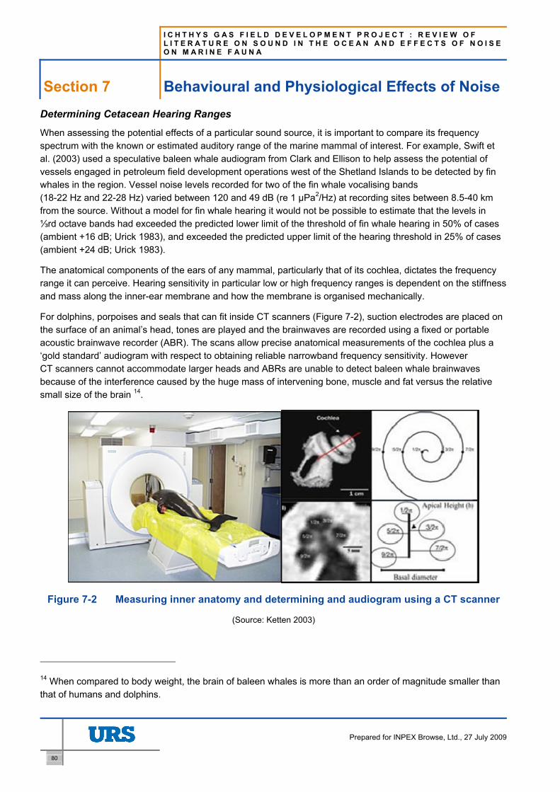
I C H T H Y S G A S F I E L D D E V E L O P M E N T P R O J E C T : R E V I E W O F L I T E R A T U R E O N S O U N D I N T H E O C E A N A N D E F F E C T S O F N O I S E O N M A R I N E F A U N A
Section 7 Behavioural and Physiological Effects of Noise
80
Prepared for INPEX Browse, Ltd., 27 July 2009
Determining Cetacean Hearing Ranges
When assessing the potential effects of a particular sound source, it is important to compare its frequency spectrum with the known or estimated auditory range of the marine mammal of interest. For example, Swift et al. (2003) used a speculative baleen whale audiogram from Clark and Ellison to help assess the potential of vessels engaged in petroleum field development operations west of the Shetland Islands to be detected by fin whales in the region. Vessel noise levels recorded for two of the fin whale vocalising bands (18-22 Hz and 22-28 Hz) varied between 120 and 49 dB (re 1 µPa2/Hz) at recording sites between 8.5-40 km from the source. Without a model for fin whale hearing it would not be possible to estimate that the levels in ⅓rd octave bands had exceeded the predicted lower limit of the threshold of fin whale hearing in 50% of cases (ambient +16 dB; Urick 1983), and exceeded the predicted upper limit of the hearing threshold in 25% of cases (ambient +24 dB; Urick 1983).
The anatomical components of the ears of any mammal, particularly that of its cochlea, dictates the frequency range it can perceive. Hearing sensitivity in particular low or high frequency ranges is dependent on the stiffness and mass along the inner-ear membrane and how the membrane is organised mechanically.
For dolphins, porpoises and seals that can fit inside CT scanners (Figure 7-2), suction electrodes are placed on the surface of an animal’s head, tones are played and the brainwaves are recorded using a fixed or portable acoustic brainwave recorder (ABR). The scans allow precise anatomical measurements of the cochlea plus a ‘gold standard’ audiogram with respect to obtaining reliable narrowband frequency sensitivity. However CT scanners cannot accommodate larger heads and ABRs are unable to detect baleen whale brainwaves because of the interference caused by the huge mass of intervening bone, muscle and fat versus the relative small size of the brain 14.
Figure 7-2 Measuring inner anatomy and determining and audiogram using a CT scanner
(Source: Ketten 2003)
14 When compared to body weight, the brain of baleen whales is more than an order of magnitude smaller than that of humans and dolphins.

I C H T H Y S G A S F I E L D D E V E L O P M E N T P R O J E C T : R E V I E W O F L I T E R A T U R E O N S O U N D I N T H E O C E A N A N D E F F E C T S O F N O I S E
O N M A R I N E F A U N A
Behavioural and Physiological Effects of Noise Section 7
Prepared for INPEX Browse, Ltd., 27 July 2009
81
The middle/inner ear complex in baleen whales is two to three times bigger than that of toothed whales, and all mysticetes studied to date have inner ears that appear well specialised for low frequency hearing. For example, Ketten (1997) deduced from comparative morphological studies of the blue whale auditory apparatus that these rorquals have good infrasonic hearing (10-20 Hz). Because there are no other humane methods for obtaining direct measurement audiograms for baleen whales, comparative anatomical modelling studies using mathematical functions have been devised (Ketten 2000).
The mathematical functions used to estimate frequency sensitivity of the humpback whale were obtained by relating the relative length of the basilar membrane with known data for cats and humans. The predicted audiogram was the typical mammalian U shape that suggested 200-10,000 Hz auditory range with maximum sensitivity between 2000-6000 Hz (e.g. Houser et al. 2001). A model of humpback hearing was subsequently created as a series of pseudo Gaussian bandpass filters. Model sensitivity optimised to the predicted audiogram by using programs to evolve the number, frequency distribution and shape of the model filters, and the sensitivity of the model was evaluated through a simulated hearing test. Maximum deviations between model sensitivity and predicted humpback whale sensitivity remained below 10%. This integrated approach provided the first predicted audiogram for humpback whales and was used to develop the first bandpass model of the humpback ear (Houser et al. 2001).
Similar comparative auditory analysis work has been undertaken to examine the capacity of right whales to hear oncoming ships (Ketten 2003), as appears to be the case by recent field studies using ship-source surrogate devices (Tyack 2003). This study included checking for the presence of pathogens in ears from stranded right whales, particularly animals showing evidence of a ship-strike. Since noise from shipping, seismic surveys and long distance sonar have all or most energies in 5-500 Hz range, these sources overlap the current estimates for the sensitive parts of the auditory range of baleen whales.
7.1.2 Sirenians Little information is available on the auditory systems of Sirenians, particularly dugongs. Manatee’s have been studied more than dugongs, with their auditory system described as a ‘low frequency’ ear with a narrow range, poor sensitivity and poor localisation ability (Richardson et al. 1995). Like cetaceans, sirenians have no pinnae and the tympano periotics are constructed of exceptionally dense bone. Manatee ear complexes are also partly fused to the inner wall of the cranium (Ketten 1998). It has been speculated that dugongs may have more sensitive hearing than manatees, however Richardson et al. (1995) notes that there isn’t any specific data to confirm this.
Studies on a West Indian manatee’s hearings sensitivity found that it heard sounds from 15 Hz to 46 kHz, with best sensitivity in the range of 6-20 kHz. This study noted that below 3 kHz the manatee was more sensitive than any other marine mammal studied at that time, with hearing extending down the infrasonic range (15 Hz). It was further noted that sensitivity was good at the best frequency of 48-50 dB (re 1 µPa), and unexpectedly good at 10-32 kHz (Richardson et al. 1995).
Some auditory evoked potential (AEP) data are also available from a West Indian manatee. This study found sensitivity of the manatee was greatest at around 1-1.5 kHz, and noticeably less sensitive at 4 kHz, and even less so at 8 kHz, However, it was noted there may have been some sensitivity up to 35 kHz. Similar sensitivities were also demonstrated in an Amazonian manatee (Ketten 1998).
There are many anecdotal reports of dugongs avoiding areas with high boat traffic, though very little research has been undertaken to investigate the sensitivity of dugongs to noise. There are also anecdotal observations which suggest that dugongs may temporarily move from an area following explosive blasting. Initial research

I C H T H Y S G A S F I E L D D E V E L O P M E N T P R O J E C T : R E V I E W O F L I T E R A T U R E O N S O U N D I N T H E O C E A N A N D E F F E C T S O F N O I S E O N M A R I N E F A U N A
Section 7 Behavioural and Physiological Effects of Noise
82
Prepared for INPEX Browse, Ltd., 27 July 2009
results into the auditory physiology and hearing sensitivity have highlighted some significant anatomical differences between manatees and dugongs, as well as between sirenians and other marine mammals (URS 2003, cited in URS 2004). The sensitive parts of their auditory range appears to be restricted to the middle frequencies (1-18 kHz) (URS 2004).
7.1.3 Marine turtles Marine turtles do not have an external hearing organ. Very few studies have been conducted on the impact of sound on turtles and their subsequent behavioural response. However, it is thought that turtle auditory perception occurs through a combination of bone and water conduction rather than air conduction.
Sea turtles have been recorded as demonstrating a startle response to sudden noises (Lenhardt et al. 1983; McCauley et al. 2000b). Their auditory sensitivity is reported to be centred in 400-1000 Hz range, with a rapid drop off in noise perception on either side of this range. This is supported by electro physical studies which have shown that the hearing range for marine turtles is approximately 100-700 Hz (McCauley 1994), with hearing ranges from 250 to 1000 Hz for loggerhead turtles (Moein-Bartol et al. 1999) and maximum sensitivity between 300 and 500 Hz for green turtles (Ridgeway et al. 1969).
Little information, however, is available regarding any reliable threshold level for the onset of behavioural effects. A trial was conducted on a caged green and loggerhead turtle with an approaching-departing single air gun. This study found that above an air gun level of 166 dB (re 1 μPa [rms]) both turtles increased their swimming activity noticeably compared to non air gun operations, and above 175 dB (re 1 μPa [rms]) their behaviour become erratic, which was concluded to be approximately equal to the point at which unrestrained turtles may show avoidance behaviour (McCauley et al. 2000b). Although turtles are often observed approaching offshore oil and gas facilities, it is possible that anthropogenic noise may cause some turtles to avoid certain areas.
In the case of pulsed low frequency sound effects on turtle nesting behaviour, nest numbers monitored on beaches near the Port of Hay Point (Queensland) before, during and after a pile-driving program lasting several months in 1996-97 were compared. Results showed no significant trend in nest numbers, indicating that the female turtles had not been particularly sensitive to this pulsed source (Dames & Moore 2000), but nest numbers were too few to provide a conclusive result.
7.1.4 Crocodiles The estuarine crocodile’s ears are located immediately behind the eyes, the eardrum protected by an elongated flap of skin. Hearing sensitivity can be altered by opening a slit in front of the flap, or lifting the flap upward. When submerged, the ears normally close, as hearing becomes secondary to the ability to feel vibrations through the water. Detectable frequencies range from below 10 Hz to over 10 kHz and sound pressure levels below 60 dB can be detected within certain bandwidths (Richardson et al. 2002).
Crocodilians have excellent hearing in air, on a par with birds and mammals. Peak sensitivities range from 100 Hz to 3 kHz, depending on the species, which coincides with the bandwidth of calls produced by juveniles (Richardson et al. 2002).
7.1.5 Sharks The range of hearing sensitivities in the bony fishes is better known than in the sharks and rays (about 80 fish species audiograms have been determined versus four for sharks and rays; the bull shark [Carcharhinus leucas], the lemon shark [Negaprion brevirostris], the horn shark [Heterodontus francisi] and the little skate

I C H T H Y S G A S F I E L D D E V E L O P M E N T P R O J E C T : R E V I E W O F L I T E R A T U R E O N S O U N D I N T H E O C E A N A N D E F F E C T S O F N O I S E
O N M A R I N E F A U N A
Behavioural and Physiological Effects of Noise Section 7
Prepared for INPEX Browse, Ltd., 27 July 2009
83
[Raja erinacea]; e.g. Casper et al. 2003, Mann et al. 2006). However all fishes tested to date appear capable of performing the same basic hearing tasks as terrestrial and marine vertebrates, such as discriminating between sounds, determining sound direction and filtering biologically relevant signals in the presence of ambient noise (Popper et al. 2003).
The best hearing sensitivity of the sharks is within the 20 Hz to 800 Hz low frequency range. In addition, sharks also have at least some ability to perceive infrasounds (0.1 Hz to 10 Hz) at particle acceleration levels from <10~6 to >10~4 ms-2 (sufficient to detect 120-180 dB [re. 1 µPa] at 0.1 Hz). Sharks appear to use infrasound to detect potential prey such as struggling fish (Popper and Fay 1999).
7.1.6 Fish The variation among fishes in respect to sensitivity to sound is immense, and is in part due to the diversity of anatomical structures involved in detection (Popper & Fay 1999). Fish that have morphological adaptations to link the otolithic hearing organs to their swim bladders or have gas filled bullae are considered ‘hearing specialists’. Audiograms of ‘hearing specialists’ show high sensitivity to sounds with sound levels as low as 60 dB (re 1 μPa) (msp to tones) across a broad frequency range. Fish of the family Clupeoidea, which includes herring (i.e. Clupea harengus) and anchovy (Engraulis australis), are examples of hearing specialists having highly specialised auditory systems (Blaxter 1980; Nedwell et al. 2004).
Many fish have a swim bladder (rather than the bulla of Clupeoidea) that is physically linked to the inner ear. The swim bladder is a gas-filled cavity that from a hearing point of view, can act to transfer an impinging sound wave’s pressure information, as driven by the swim bladder, to the fish ear end organs or otolith systems (Popper and Fay 1993).
Fish with the prootic bulla generally have higher sensitivity than those with a swim bladder, and those with a swim bladder usually have greater sensitivity than non-specialists with no swim bladder (Nedwell et al. 2004).
Syngnathid species, including members of the pipefish and seahorse families, are listed under the EPBC Act, and are ‘hearing generalists’ meaning that they do not have any auditory specialisations that confer sensitive hearing abilities. They possess a swim bladder that is used for both communication and buoyancy. It is the swim bladder of the fish, which is a gas containing organ that will expand and contract with a rapidly changing acoustic field and as a result may cause physical injury which can result in death. For the Syngnathidae the important metric when determining the susceptibility to physical injury is its body mass. It is therefore the hatchlings that will be the most susceptible to physical injury from a pressure wave.
The capacity for hearing in Syngnathid is not well understood. There are no known audiograms of Syngnathids. Many Syngnathids have been documented to produce sound (loud clicks), suggesting that sound is important for communication in the aquatic environment (Bergert & Wainwright 1997; Colson et al. 1998; Ripley & Foran 2006). The function of clicks may be associated with mating, to coordinate spawning (to signal readiness and orientation of mates), or to advertise prey availability. Among these contexts, feeding clicks are the most widely noted. For two species of seahorse studied, peak frequency measurements were highest between 2650 to 3430 Hz for dwarf seahorse (Hippocampus zosterae), and 1960 to 2370 Hz for lined seahorse (Hippocampus erectus) (Colson et al. 1998). The frequency of noise making suggest that hearing sensitivity is the greatest in the higher frequency ranges and, by extension that the least sensitivity is in the lower frequency range. Therefore is considered that any Syngnathids exposed to noise below 180 dB (re 1 µPa) are unlikely to be significantly effected.

I C H T H Y S G A S F I E L D D E V E L O P M E N T P R O J E C T : R E V I E W O F L I T E R A T U R E O N S O U N D I N T H E O C E A N A N D E F F E C T S O F N O I S E O N M A R I N E F A U N A
Section 7 Behavioural and Physiological Effects of Noise
84
Prepared for INPEX Browse, Ltd., 27 July 2009
There have been very few studies of the effects of anthropogenic sounds on the behaviour of fishes. Data are lacking not only on the immediate behavioural effects on fishes close to a source, but also effects on fishes further from the source Several studies have demonstrated that human-generated sounds may affect the behaviour of at least a few species of fish (Table 7-1).
Table 7-1 Citations of selected studies examining the effects of exposure to sound on fishes that have most relevance to pile driving.
Issue Hearing Generalists Hearing Specialists
Mortality Yelverton et al. 1975 (guppy, bluegill, trout, bass, carp; explosive blasts).
Yelverton et al. 1975 (goldfish, catfish, minnow; explosive blasts).
Hastings 1995 (goldfish and gouramis; pure tones).
Physical Injury Yelverton et al. 1975 (guppy, bluegill, trout, bass, carp; explosive blasts).
Govoni et al. (2003) (larval fish; explosive blasts, no pathology seen).
Yelverton et al. 1975 (goldfish, catfish, minnow; explosive blasts).
Hastings 1995 (goldfish and gouramis; pure tones).
Auditory Tissue Damage
Enger 1981 (cod; pure tones, 1 – 5 hr)
Hastings et al. 1996 (oscar; pure tones, 1 hr).
McCauley et al. 2003 (pink snapper, air gun).
Hastings 1995 (goldfish; pure tones, 2 hr).
Permanent Threshold Shift (PTS)
No data available. No data available.
Temporary Threshold Shift (TTS)
No relevant data available. Smith et al. 2004 a, b (goldfish; band-limited noise).
Scholik and Yan 2001 (fathead minnow; band-limited white noise).
Popper and Clarke 1976 (goldfish; pure tones).
Popper et al. 2005 (northern pike, lake chub).
Behavioural Changes
Wardle et al. 2001 (Exposed fish and invertebrates on reef to continuous air gun with no significant behavioural changes).
McCauley et al. 2000b (Experimental air gun trials with fish initially showing behavioural changes).
No data available.

I C H T H Y S G A S F I E L D D E V E L O P M E N T P R O J E C T : R E V I E W O F L I T E R A T U R E O N S O U N D I N T H E O C E A N A N D E F F E C T S O F N O I S E
O N M A R I N E F A U N A
Behavioural and Physiological Effects of Noise Section 7
Prepared for INPEX Browse, Ltd., 27 July 2009
85
Issue Hearing Generalists Hearing Specialists
Eggs and Larvae Banner and Hyatt 1973 (Cyprinidon and Fundulus showed somewhat decreased egg viability and larval growth in tanks with increased noise).
Kostyuchenko 1973 (Increased egg mortality up to 20 m from seismic source).
Booman et al. 1996 (Variable results with some stages showing decreased growth in a few species when exposed to air guns).
No data available.
Miscellaneous Skalski et al. 1992 (Sebastes catch decreased after one air gun blast).
Engås et al. 1996 (Haddock and cod catch reduction after seismic survey blasts).
Engås and Løkkeborg 2002 (Haddock and cod catch reduction area after seismic survey blast.
Slotte et al. 2004 (herring & blue whiting do not enter the area of air gun during use).
Smith et al. 2004a (no change in corticosteroid levels after continuous exposure to band limited noise).
While not totally germane to fishes, there is some evidence that an increased background noise (for up to three months) may affect at least some invertebrate species. Legardère (1982) demonstrated that sand shrimp (Crangon crangon) exposed in a sound proof room to noise that was about 30 dB above ambient for three months demonstrated decreases in both growth rate and reproductive rate. In addition, Legardère and Régnault (1980) showed changes in the physiology of the same species with increased noise, and that these changes continued for up to a month following the termination of the signal.
Indeed, we are now aware that fishes, as mammals and probably all other vertebrates, glean a great deal of information about their environment from the general sound field. In other words, whereas visual signals are very important and useful for things near the animal and in the line of sight, substantial information about the unseen part of an animal’s world comes from acoustic signals.
One may therefore think of fishes as using two “classes” of sound. The first is the well-known group of communication signals used to keep in touch with other members of a species and detect the presence of predator or nearby prey. The second are the sounds of the environment that, for a fish, might include the sounds produced by water moving over a coral head, waves breaking on shore, rain, and many more physical and biological sources. Bregman (1991) coined the term “Auditory Scene” to describe the acoustic environment.
The acoustic environment has become of increasing importance in the overall understanding of hearing for all animals during the past 15 years. Moreover, it is becoming increasingly clear that one of the major roles of the auditory system is to discriminate between, and determine the position, of sounds in the auditory scene, using a mechanism called “stream segregation” (Bregman 1991; Fay and Popper 2000; Popper et al. 2003) whereby an organism is able to distinguish between two sounds (“streams”) that differ in some way such as direction of the source, frequency spectrum, etc.

I C H T H Y S G A S F I E L D D E V E L O P M E N T P R O J E C T : R E V I E W O F L I T E R A T U R E O N S O U N D I N T H E O C E A N A N D E F F E C T S O F N O I S E O N M A R I N E F A U N A
Section 7 Behavioural and Physiological Effects of Noise
86
Prepared for INPEX Browse, Ltd., 27 July 2009
Interim criteria for injury of fish exposed to pile driving operations
Popper et al.(2006) undertook an extensive review of literature with the aim of determining noise exposure criteria for the onset of direct physical injury in fish exposed to the impact sound associated with pile driving.
When proposing these criteria, Popper et al. (2006) recognised that fish may respond to noise from pile driving without actually experiencing injury. However, they do not propose criteria for behavioural responses or other sub-injurious auditory effects, and believe this not possible at present, due to the absence of relevant data. Furthermore, it is recognised that conservative decisions were made where data are lacking, and therefore the interim criteria proposed are set at precautionary levels, and exposure thresholds are somewhat lower than present literature may suggest as the levels that would result in the onset of injury.
Based on the best available science at the time of development, Popper et al. (2006) believe it reasonable and appropriate to use a dual criteria approach, and propose that the interim criteria for the onset of direct physical injury to fish exposed to pile driving be set at a sound exposure level of 187 dB (re 1 µPa2.sec) and a peak sound pressure level of 208 dB (re 1 µPapeak). In adopting the dual criteria approach, it is intended that the sound exposure level criterion limits the total acoustic energy fish may experience within a single impulsive sound, while the peak sound pressure level protects fish from an especially strong excursion in pressure within the sound impulse. For these reasons Popper et al. (2006) recommend both criteria be implemented during pile driving activities and neither should be exceeded.
In selecting the interim criteria, Popper et al. (2006) relied upon four studies (Yelverton et al.1975, Caltrans 2004, Popper et al.2005 & Popper et al., in prep), only one of which (Popper et al. in prep [unpublished]) was related directly to pile driving, the others concerning effects from explosions, seismic airguns and sonar. However, in respect of biological consequences, Popper et al. (2006) believe that the source of the energy which may affect exposed fish is not important, rather it is the received exposure conditions (attributable to the particular characteristics of a signal of interest), the specific environment in which the sound is produced and the physical orientation of the source and receiver which is important. Popper et al. (2006) also believe there are other salient factors determining acoustic effects, including the rise time of the signal, the number of exposures of an animal to a particular signal, the time between each exposure, and the physiological accumulation of effects.
When considering potential physical effects from pile driving, Popper et al. (2006) also recognise that specific effects depend on a broad range of factors, including the type of pile, type of hammer, substrate, actual species of fish and environmental setting.
7.2 Categories of Sound Impacts Reviews such as Richardson et al. (1995), Gisiner (1998), McCauley and Cato (2003) and URS (2003) note how sound waves from nearby, discernible sound sources affect marine mammals differently to those from distant, undiscernible ships and other low frequency sources which add to background ambient noise.
Development of Harbour facilities serviced by heavy vessel traffic will also elevate local background levels, and may cause some species to avoid former nearby breeding or feeding areas owing to the amount of vessel movement disturbances as well as the noise. For example, gray whales temporarily abandoned a breeding lagoon in Baja, California, during a period of extensive coastal industrial activity involving heavy vessel traffic. The whales did not return to the lagoon until the vessel activity had decreased (Gard 1974).While some marine

I C H T H Y S G A S F I E L D D E V E L O P M E N T P R O J E C T : R E V I E W O F L I T E R A T U R E O N S O U N D I N T H E O C E A N A N D E F F E C T S O F N O I S E
O N M A R I N E F A U N A
Behavioural and Physiological Effects of Noise Section 7
Prepared for INPEX Browse, Ltd., 27 July 2009
87
mammals can appear more capable of habituating to such activities than others (such as dolphins in noisy urbanised estuaries and embayments, and sperm whales feeding in busy shipping lanes), their calving or pupping areas are almost invariably restricted to far less disturbed locations.
The above effects are due to essentially permanent vessel traffic and other noise generating activities. These are not addressed in the following sub-sections, which focus on the effects of noise from discernible sources generated by relatively short-term human activities (as summarised in Table 7-2).
Different types of noise can be broadly categorised as follows:
• Continuous or near-continuous sources that may prevent marine mammals or turtles from hearing social communications or other acoustic cues (= temporary masking effects).
• Noise that induces behavioural changes and responses in marine mammals and turtles.
• Noise that induces behavioural responses by the prey of toothed whales (fish, cephalopods).
• Very intense noise that may cause temporary or possibly permanent loss of hearing sensitivity to marine mammals via damage to the auditory hair cells (or other tissue trauma via possible excitatory and organ resonance mechanisms).
To assess the potential scale and likelihood of these effects, ‘safety ranges’ or zones of influence have been developed for predicting, measuring and managing noise-generating activities, in the same way that zones of lethality 15 have been used for assessing the spatial extent of possible marine animal injuries from the non-acoustic blast impulses of underwater explosions.
15 The maximum amplitudes of acoustic waves that do not contain sufficient energy to kill, maim or stun marine mammals or turtles outright (e.g. Lewis 1996b, Richardson et al. 1995, URS 2003).

I C H T H Y S G A S F I E L D D E V E L O P M E N T P R O J E C T : R E V I E W O F L I T E R A T U R E O N S O U N D I N T H E O C E A N A N D E F F E C T S O F N O I S E O N M A R I N E F A U N A
Section 7 Behavioural and Physiological Effects of Noise
88
Prepared for INPEX Browse, Ltd., 27 July 2009
Table 7-2 Summary characteristics of some common human sound sources
Source Perceived location/s
Perceived speed and direction of source Sound periodicity Frequency
range (Hz) Source Level1
Seismic airgun array Moving Slow (4-6 knts) and steady direction
Very regular short pulses
LF (8-1000) Most <500
215-2403
(ramped)Well drilling Fixed Fixed Steady continuous Tonals 130-150 Field development support vessels Almost fixed Slow with
variable direction Irregular periods of
continuous or transients LF + tonals 170-190
Trading ships Moving Fast (12-22 knots) and steady Steady continuous LF (10-500) +
tonals (1 kHz) 160-186
Whale watching vessels2
Multiple, moving
Variable speeds and directions
Variable (continuous and transients)
LF-MF + HF tonals 140-190
Pile driving Fixed Stationary Irregular periods of regular pulses LF-MF tonals 170-180
Detonations4 Unpredicted N/A Unpredictable sudden short pulse Wideband 240-260
Dredging Fixed Stationary Variable continuous sounds
LF-MF + tonals 150-195
Sea dumping Unpredicted Stationary, or slow with variable direction
Unpredictable sudden transients (2-10 mins) LF-MF 140-190
MF tactical sonar Multiple and moving Erratic Unpredictable sudden
short pulses MF
(2-10 kHz) 200-225
LF surveillance sonar Moving Slow and steady Regular long pulses LF (100-400) 230-235 (ramped)
NPAL research sonar Fixed Stationary Regular 20 minute pulses LF (40-300) 195 (ramped)
1) dB (re 1 μPa @ 1m) / dB (re 1 μPa 2 @ 1m) msp.
2) small ferries, launches, outboard RHIBS, various recreational.
3) for 2,000-2,800 cubic inch arrays in Aus. waters.
4) e.g. rock blasting, hulk scuttling, removals, bay cable survey.
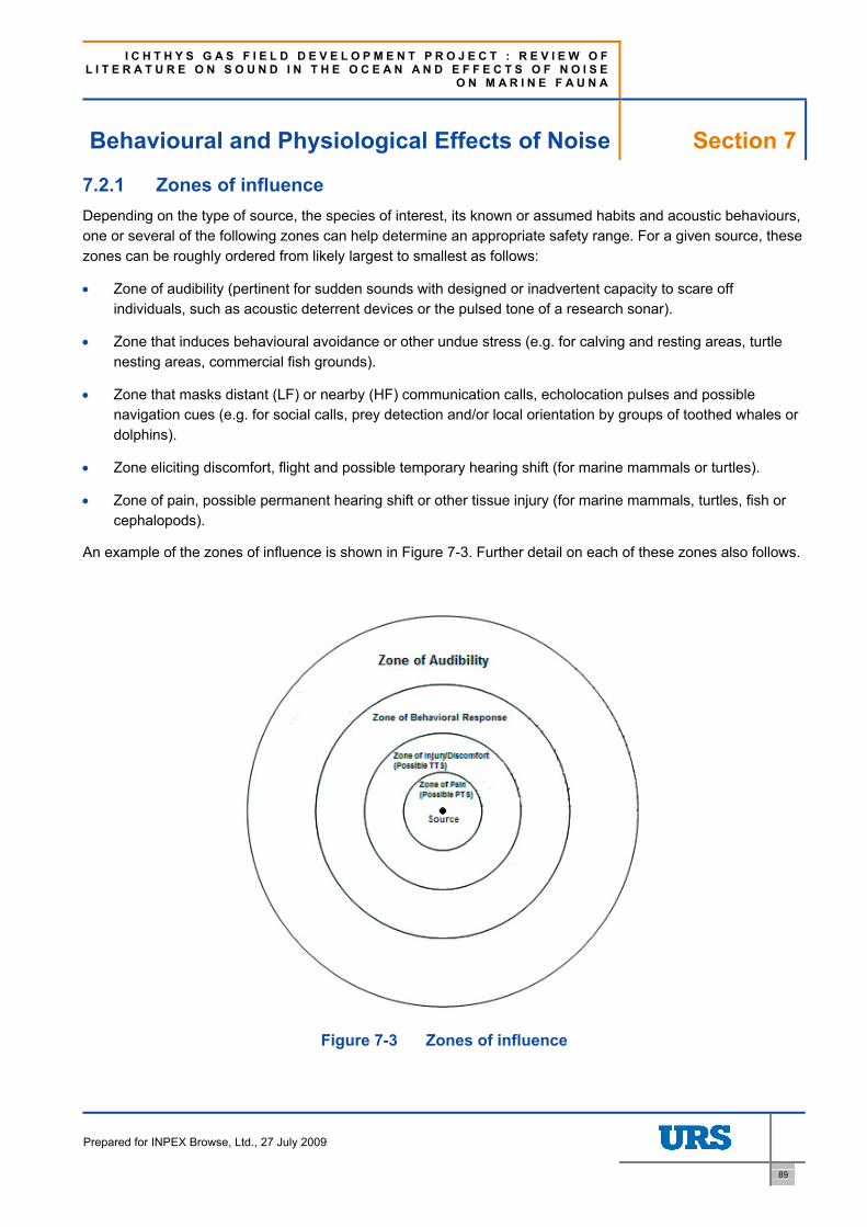
I C H T H Y S G A S F I E L D D E V E L O P M E N T P R O J E C T : R E V I E W O F L I T E R A T U R E O N S O U N D I N T H E O C E A N A N D E F F E C T S O F N O I S E
O N M A R I N E F A U N A
Behavioural and Physiological Effects of Noise Section 7
Prepared for INPEX Browse, Ltd., 27 July 2009
89
7.2.1 Zones of influence Depending on the type of source, the species of interest, its known or assumed habits and acoustic behaviours, one or several of the following zones can help determine an appropriate safety range. For a given source, these zones can be roughly ordered from likely largest to smallest as follows:
• Zone of audibility (pertinent for sudden sounds with designed or inadvertent capacity to scare off individuals, such as acoustic deterrent devices or the pulsed tone of a research sonar).
• Zone that induces behavioural avoidance or other undue stress (e.g. for calving and resting areas, turtle nesting areas, commercial fish grounds).
• Zone that masks distant (LF) or nearby (HF) communication calls, echolocation pulses and possible navigation cues (e.g. for social calls, prey detection and/or local orientation by groups of toothed whales or dolphins).
• Zone eliciting discomfort, flight and possible temporary hearing shift (for marine mammals or turtles).
• Zone of pain, possible permanent hearing shift or other tissue injury (for marine mammals, turtles, fish or cephalopods).
An example of the zones of influence is shown in Figure 7-3. Further detail on each of these zones also follows.
Figure 7-3 Zones of influence

I C H T H Y S G A S F I E L D D E V E L O P M E N T P R O J E C T : R E V I E W O F L I T E R A T U R E O N S O U N D I N T H E O C E A N A N D E F F E C T S O F N O I S E O N M A R I N E F A U N A
Section 7 Behavioural and Physiological Effects of Noise
90
Prepared for INPEX Browse, Ltd., 27 July 2009
7.2.2 Zone of audibility The zone of discernible audibility represents the maximum possible radius of influence by a particular source. This range can vary markedly according to the species and individuals of interest, plus their specific location, source-receiver-seabed geometry, season and time of day. Factors which can cause the boundary of these zones to expand and contract on an almost moment by moment basis include:
• the frequency, temporal characteristics, directionality, depth and orientation of the source
• the host of physical factors dictating the transmission loss rate and propagation of the peak frequency band/s towards the receiver
• the particular depth of the receiving individuals of interest and their hearing thresholds with respect to the peak frequency components of the source’s bandwidth
• the levels of the various physical, biological and other human sources that form the ambient noise intensity spectrum at the receiver’s location
• the level of attention and habituation (previous signal experience) of the receivers, which will influence their ability and motivation to perceive and interpret the signal.
Many of the above factors can vary minute by minute as well as differ substantially between regions and locations, and thus limit the significance and value of determining this zone for most sources and species. Nevertheless estimates of maximum audibility of specific noise sources are occasionally reported for marine mammals with known or estimated spectral audiograms and hearing thresholds. For example, the absolute auditory threshold to a 1000 Hz tone for a captive beluga whale has been measured as 104 dB (re 1 µPa). The critical signal to noise ratio (SNR) at this frequency (i.e. the amount by which the signal must exceed background noise to become audible) was determined to be 17 dB.
Such measurements imply that beluga whales experiencing typical arctic ocean ambient noise conditions cannot detect icebreaker noise at ranges beyond 20 km, even at full power (Table 7-2). This example contrasts with earlier findings by Finley et al. (1990), who had previously attributed a substantial movement of beluga whales to avoid icebreaker noise. In this case, the beluga whales were reported to stop feeding and swim away from approaching icebreakers, travelling up to 80 km from feeding areas before returning after 1-2 days (Finley et al. 1990). The apparent contradictory evidence highlights the problem of attributing cause/effects in field conditions where the auditory sensitivity is unclear and where control examples are unavailable or involve different conditions.
For cases involving the maximum audibility of continuous or regular periods of low broadband noise (such as the sound of distant shipping traffic, a slow-moving icebreaker or a stationary drilling operation), there is little in the weakly discernible signals to invoke a particular behavioural effect, learned or otherwise, and the issue turns toward masking effects. In the case of repetitive short pulses of low frequency sound from distant airgun or pile driving sources, their pulsed nature would make them more readily perceivable at long distance, but the separation of the weak and distant pulses by intervals of many seconds (typically >10) lessens their ability to mask out any long distance calling sequences of the larger rorquals (which last >20 seconds or, in the case of humpbacks, many minutes; Section 5.2.6). Sources that propagate near continuous and essentially non discernible broadband sound contribute to ambient noise, and it is more useful to assess their capacity to mask incoming sounds and cues of import to local receivers.

I C H T H Y S G A S F I E L D D E V E L O P M E N T P R O J E C T : R E V I E W O F L I T E R A T U R E O N S O U N D I N T H E O C E A N A N D E F F E C T S O F N O I S E
O N M A R I N E F A U N A
Behavioural and Physiological Effects of Noise Section 7
Prepared for INPEX Browse, Ltd., 27 July 2009
91
The audible zone has more relevance for acoustic deterrent or harassment devices which emit aperiodic pulsed signals as these have the capacity to startle marine Fauna, as could the sudden appearance of a research or military sonar tone. Thus the value of assessing a source’s audible range increases (a) the more its signal is readily distinguishable from ambient background and (b) the more likely the characteristics of this signal will invoke interpretation and potentially adverse responses by individuals of the species of interest. This switches our attention to zones which induce behavioural reactions to noise such as the startle response and avoidance. These ranges are also more amenable to monitoring and mitigation.
7.2.3 Zone of behavioural responses The zone of behavioural response is logically smaller than the zone of audibility, and is based on the received sound level which evokes changes in behaviour that may result in adverse effects on the well-being of individuals and populations of protected species.
The capacity of an unmanaged sound source to cause startle responses, or other types of undue interference and stress that may lead to biologically significant consequences to a protected marine species, varies markedly according to the source characteristics. Not all human sounds cause undue behaviour responses, and some are more amenable to habituation than others. Sound source features which increase a source’s capacity to receive attention from and interfere with marine mammals or turtles engaged in feeding, breeding or resting activity are summarised in Table 7-2.
The types of observable reaction have depended on the nature and affordability of the particular physiological or behavioural responses that can be measured in research aquaria (i.e. for captive dolphins or the occasional small toothed whale) or observed visually and/or acoustically in natural open waters for the larger whales. Field methods are constrained by the availability, amenability and ‘repertoire’ of measurable behaviours of the species of interest, while both field and laboratory studies are constrained by ethical considerations regarding the effect of deliberate sound exposures to the welfare of tested subjects16.
16 There has been development of increasingly sophisticated and affordable digital telemetry acoustic tags (DTAGs) which can be temporarily attached to large whales in open waters by suction cap (some with depth and inertial motion detectors for diving studies or positioning systems for satellite monitoring). This is widening the number of observable responses that previously were constrained to captive dolphins or small odontocete whales within the confines of research aquaria.

I C H T H Y S G A S F I E L D D E V E L O P M E N T P R O J E C T : R E V I E W O F L I T E R A T U R E O N S O U N D I N T H E O C E A N A N D E F F E C T S O F N O I S E O N M A R I N E F A U N A
Section 7 Behavioural and Physiological Effects of Noise
92
Prepared for INPEX Browse, Ltd., 27 July 2009
Table 7-3 Features of an audible source likely to increase level of attention and invoke behavioural responses in marine fauna
Source characteristic Increased biological significance Response
Frequency range Within sensitive part of receiver’s auditory range
Narrowband signal Easier to detect (>SNR*); imparts potential meaning
Pulsed signal Easier to perceive, potentially disruptive
Moving Invokes more attention (e.g. vectoring to discern direction)
Increasing
attention / curiosity
Sudden / aperiodic Increases likelihood of causing a startle response
Moving fast (>10 knots) Increases chance of alarm and flight unless the source is common with steady direction (habituation effect)
Position or heading Between receiver and its intuitive pathway to safety Erratic direction and speed Unpredictable movements invoke continual vectoring, sense of
alarm, disengagement of previous activities, avoidance/defensive reactions.
Increasing
stress/alarm
* = Signal to (ambient) Noise Ratio
Behavioural reactions to sound vary with the species and individuals of interest, including their state of attention and activity, maturity, experience and parental duty, all of which will alter with season, location and times of day, etc. Reactions involving relatively small avoidance responses by individuals are clearly not biologically significant, whereas those produced in scenarios involving a near permanent sound source which may displace animals from key feeding or breeding grounds over monthly or seasonal time scales would have obvious import to growth, stress levels, breeding success, survivorship and population recovery rates.
A range of surface-visible and acoustic behaviour features of cetaceans have been monitored as direct or surrogate measures of potentially adverse responses to the onset or approach of a sound source (or its surrogate device). The level of success of these studies has been shown to be highly dependent on weather conditions, animal abundance and activity, and/or the appearance of unanticipated confounding factors. In addition, these factors, versus the amount of available study time, observation platform/s, reliable hydrophone systems and field personnel, also affect the overall level of success.

I C H T H Y S G A S F I E L D D E V E L O P M E N T P R O J E C T : R E V I E W O F L I T E R A T U R E O N S O U N D I N T H E O C E A N A N D E F F E C T S O F N O I S E
O N M A R I N E F A U N A
Behavioural and Physiological Effects of Noise Section 7
Prepared for INPEX Browse, Ltd., 27 July 2009
93
Behavioural changes monitored during open water studies of specific sound sources typically include one or more of the following (depending on the particular source, species and the level of activity of the individuals 17 at the location of interest):
• course alterations to directions away from or towards the source and speed changes
• cessation or change to previous activity
• altered local/regional distribution patterns of individuals/groups (typically by aerial survey)
• close up (bunching) of group members or pairs
• alterations to cow-calf interactions
• alterations to surfacing interval and/or number of breaths between dives
• absence of ‘fluke ups’ (marking feeding dives in some species)
• alterations to dive patterns and durations
• alteration of call type, rate, duration, depth and timing
• alteration of echolocation rate, type, duration, depth and timing
• changes to spy-hopping, breaching or fin slap rates (interpreted as evidence of curiosity, defensive or annoyance behaviours respectively).
For any given location and propagation conditions, the range at which the received sound of a source invokes a behavioural response will depend on the auditory sensitivity of the species of interest, while the biological significance of this response will vary according to the type of activity being undertaken. Not all behaviour responses increase risk of harm to individuals, breeding success or population recovery rates. Some responses may be momentary inconsequential reactions such as the turn of a head, or have limited duration and lie within the bounds of natural behaviour variations. Table 7-3 summaries the potential significance of possible diverted attention, avoidance and alarm responses by large whales as a result of a human noise source, in the context of feeding, migrating, resting, calving or mating activities.
Early studies had pointed to the baleen whales and possibly sperm whales as the most seismic survey sensitive of marine mammals in terms of behavioural responses and the eared seals and sea lions (Otarids) as the least sensitive (Richardson et al. 1995). Work during and since the 1990s has shown this generalisation is not uniform and is untrue for sperm whales (e.g. Madsen et al. 2003, Richardson et al. 1999, Stone 2003).
7.2.4 Zone of potential masking Zones of masking depend on the amount of overlap between received source peak frequencies and the communication band/s of the species in question, plus the proximity of habitat deemed critical to the conservation and well-being of its local population or regional stock. As noted in Section 7.2.2, examining the potential of a near continuous low frequency broadband source to mask long distance communications is more
17 Whales engaged in an intensive activity such as feeding are generally more preoccupied and less responsive to external stimuli and cues than when inactive, resting or migrating (Richardson et al. 1995).

I C H T H Y S G A S F I E L D D E V E L O P M E N T P R O J E C T : R E V I E W O F L I T E R A T U R E O N S O U N D I N T H E O C E A N A N D E F F E C T S O F N O I S E O N M A R I N E F A U N A
Section 7 Behavioural and Physiological Effects of Noise
94
Prepared for INPEX Browse, Ltd., 27 July 2009
useful than estimating its maximum discernible audible range, particularly for a whale frequented locality already experiencing elevated background noise levels from other human sources.
Table 7-4 Type and possible consequences of behaviour changes from exposure to human noise source*
Activity Possible Effect / Response Potential Consequence Significance*
Intense feeding on important but possibly ephemeral or seasonally restricted prey
Influences normal diving and recovery sequences, group working, use of echolocation, or causes other behaviour change that reduces feeding
Reduced feeding efficiency causes reduced net energy intake (size of reduction depends on number and duration of encounters)
Low if encounters are brief and few. If prey is limiting, increases with percent of feeding time affected. May stabilise if habituation occurs.
Long distance migration to/from feeding ground
Alter course to avoid source
Course deviations involving +10 km add a fraction of time and energy loss to the overall journey budget of >2000 km
Low (equivalent to detouring around the approaches to a busy port)
Resting
Increased sensitivity to novel or unexpected noise reduces sound level tolerance. Forced to move away from source.
Unplanned exertion and use of energy
Increases with number of disturbances before or after calving
Calving
Increased stress, avoidance or defensive behaviour increases risk of injury to calf and cow
Disrupted birthing or suckling increases risk of cow/calf injury, calf oxygen debt, reduced milk intake, exposure to predators.
Risk of mortality increases with number of interactions (risk of reduced population recovery rate).
Social interactions and mating in winter breeding grounds
Diverted attention, disrupted vocalisations, and/or avoidance behaviour disrupts mate selection, courtship and mating.
Reduction in factors facilitating adequate insemination, conception and embryo implantation.
As above, with respect to reduced pregnancy rate.
* Assumes exposure to a novel noise source. May stabilise/reverse if the characteristics and commonality of the particular source facilitate habituation.
Both toothed and baleen whales have been observed to respond to increased background noise by producing more calls, louder calls, longer calls and/or shifting call frequencies. In the case of dolphins and toothed whales, these tend to remain in large family groups, specialise in high frequency (short-distance) vocalisations and do not generate low frequency sounds capable of long distance communication. In noisy localities and embayments bottlenose dolphins have been shown to echolocate louder (Au & Penner, 1981) and change the frequency characteristics of their whistles and echolocation clicks (Au et al. 1974, plus recent Hervey/ Moreton/Port Philip Bay comparative studies).

I C H T H Y S G A S F I E L D D E V E L O P M E N T P R O J E C T : R E V I E W O F L I T E R A T U R E O N S O U N D I N T H E O C E A N A N D E F F E C T S O F N O I S E
O N M A R I N E F A U N A
Behavioural and Physiological Effects of Noise Section 7
Prepared for INPEX Browse, Ltd., 27 July 2009
95
7.2.5 Zone-inducing possible temporary threshold shifts in hearing When exposed to a sufficiently intense sound source, the inner ear hair cells of marine mammals can receive excessive excitation and subsequently cause a temporary decline in hearing sensitivity, in the same way as land mammals and humans. This is called a ‘temporary threshold shift’ (TTS), and its appearance due to the ‘tiring out’ of the hair cells is a function of the strength of the sound and duration of exposure. In the case of human health and safety regulations, the typical workplace regulations to prevent TTS via 8 hour shift exposures are 80 or 90 dB (re 20 μPa), which are equivalent to underwater levels of roughly 142 to 152 dB (re 1 μPa).
While the potential for TTS to occur in marine mammal ears has been recognised for several decades, reliable data regarding the sound levels inducing TTS did not begin to emerge until the late 1990s. Before these results, expert opinion sought by the US NMFS (e.g. HESS 1999, US Marine Mammal Commission 2004) had indicated that, for precautionary reasons including possible TTS, cetaceans should not be exposed to pulsed underwater noise at received levels exceeding 180 dB and 190 dB (re 1 µPa) (rms) respectively. The more recent studies have since identified that pulsed sounds which cause mild TTS in dolphins and small toothed whales need to exceed >200 dB (re 1 µPa) (rms) (e.g. Schlundt et al. 2000, Finneran et al. 2002; refer Figure 7-3). More recent work by Southall et al. (2007) indicates higher received levels for TTS onset (see section 7-3).
The TTS threshold is a time versus energy exposure function of the received sound, with the measured loss in hearing sensitivity (3-6 dB at or just above the frequency of the received sound) related to the total received energy (e.g. Finneran et al. 2002). When a TTS is present, the hearing threshold rises and a sound must be stronger in order to be heard. A TTS typically lasts for minutes, but may extend to hours or even days in cases of a strong TTS. The affected region remains at and just above the frequency range of the offending TTS causing sound.
Repeated TTS events without sufficient intervening recovery periods can lead to irreparable damage to the hair cells, thereby leading to a Permanent Threshold Shift (PTS; Section 6.2.6). The potential significance of TTS to long lived mammals such as the larger whales is therefore twofold: a temporary period when the ability to perceive a social signal, echolocation image or orientation cue may be impaired, plus an increase in the long term risk of accelerated hearing loss in old age. However, as with humans and terrestrial mammals, the auditory system is resilient and can experience the occasional TTS without undue risk of PTS developing. Thus some workers maintain that mild TTS is not injury per se, as it is a natural phenomenon experienced by humans and terrestrial mammals and has also been shown in marine fauna. In this context, there are a range of natural sources that can emit intense LF, MF and/or HF sounds that, during the lifespan of a larger whale, could be capable of producing a mild TTS (Table 7-1).
Since the capacity of neonates and young juveniles to receive several TTS with the same likelihood of avoiding an early onset of PTS is unclear, the biological significance of TTS-inducing levels is arguably higher in calving areas and for cow-calf pairs on their first migration to feeding grounds.
Recent laboratory results of TTS testing in delphinid species indicate the received level of a single seismic pulse needs to be ~210 dB (re 1 µPa) rms (approx. 221-226 dB (re 1 µPa) peak-peak) to induce brief TTS (i.e. minutes of reduced hearing sensitivity). Exposure to several seismic pulses over a 30-60 minute period may require received levels of 200-205 dB rms) to cause the same level of TTS in a dolphin or small toothed whale. Exposure levels inducing a mild TTS by typical seismic survey sounds (i.e. a series of very short pulsed sounds each separated by 8-15 second intervals) have not been determined, but can be assumed to be the roughly the

I C H T H Y S G A S F I E L D D E V E L O P M E N T P R O J E C T : R E V I E W O F L I T E R A T U R E O N S O U N D I N T H E O C E A N A N D E F F E C T S O F N O I S E O N M A R I N E F A U N A
Section 7 Behavioural and Physiological Effects of Noise
96
Prepared for INPEX Browse, Ltd., 27 July 2009
same as the values inducing TTS reported for short (1 second) pulses (e.g. Finneran et al 2002) versus the long exposure periods (>20 minutes) (e.g. Nachtigall et al. 2003).
The ability of the 5-15 second inter-pulse intervals to provide an ameliorative ‘mini’ recovery phase may be low. Nevertheless, the zone of potential temporary hearing loss and discomfort near an airgun array is relatively small, with geometrical spherical spreading causing a decline in sound levels to <200 dB (re 1 µPa) within 500 m of the largest commercial arrays.
Figure 7-4 Plot indicating sound exposure regimes (s) and energy flux densities (b) that can induce measurable TTS in odontocetes
(from Finneran et al. 2002)
Most experiments on TTS have been undertaken on bottlenose dolphins and beluga whales. The test tones were in the range of 40 to 7500 Hz with levels up to 202 dB (re 1 μPa) (Schlundt et al. 2000). Evidence of TTS was obtained, disappearing within a few days. The following account summarises the methods and findings of TTS experiments reported by Finneran et al. (2002). A behavioural response paradigm was used to measure masked underwater hearing thresholds in a bottlenose dolphin (Tursiops truncatus) and a beluga whale

I C H T H Y S G A S F I E L D D E V E L O P M E N T P R O J E C T : R E V I E W O F L I T E R A T U R E O N S O U N D I N T H E O C E A N A N D E F F E C T S O F N O I S E
O N M A R I N E F A U N A
Behavioural and Physiological Effects of Noise Section 7
Prepared for INPEX Browse, Ltd., 27 July 2009
97
(Delphinapterus leucas) before and after exposure to single underwater impulsive sounds produced by a seismic watergun 18.
Pre- and post exposure thresholds were compared to determine if a temporary shift in masked hearing thresholds (MTTS), defined as a 6 dB or larger increase in the post exposure threshold, had occurred. Hearing thresholds were measured at 400 Hz, 4000 Hz and 30 kHz. MTTSs of 7 and 6 dB were observed in the beluga at 400 Hz and 30 kHz respectively, for approximately 2 minutes after exposure to single impulses with peak pressures of 160 kPa, peak-to-peak pressures of 226 dB (re 1 µPa) and total energy fluxes of 186 dB (re 1 µPa2 s). Thresholds returned to within 2 dB of the pre exposure value approximately 4 minutes after exposure. No MTTS was observed in the dolphin at the highest exposure conditions: 207 kPa peak pressure, 228 dB (re 1 µPa) peak to-peak pressure, and 188 dB (re 1 µPa2 s) total energy flux.
Finneran et al. (2002) also compared their findings with results from other TTS studies using different sound exposure regimes (Figure 7-3). The plots show that inducing TTS in cetaceans involves a sound dosage function in which the critical energy flux density for species tested to date is above 185 dB (re 1 µPa2 sec-1). There are no measured data on sound levels that induce TTS in baleen species.
7.2.6 Zone-inducing possible permanent threshold shift or other tissue damage
PTS results from irreparable injury to the hair cell receptors that line the basement membrane of the inner ear (unlike birds and reptiles, these are not replaced during adult mammal life). If relationships between TTS and PTS thresholds in marine mammals are similar to those studied in humans and other terrestrial mammals, PTS requires an exposure to ~20 dB higher peak to peak sound pressure levels than TTS.
Extreme PTS cases involve partial or total deafness that occurs by exposure to non-acoustic blast pressures, i.e. via proximity to detonations of high explosives. Exposure to explosive energies causes PTS owing to the more rapid rise time of the blast pressure wave (i.e. microseconds versus the milliseconds of airgun pulses). Humans and mammals with a PTS have continually impaired ability to hear sounds over various frequency ranges, which widen and worsen in older life, particularly for the higher frequencies.
If marine mammals have an inherently high behavioural tolerance to intense levels of pulsed noise (~200 dB (re 1 μPa rms), this does not necessarily mean their hearing sensitivity may not become impaired over the long-term. For example, McCauley and Duncan (2001) have noted that while humans can tolerate short, repetitive explosive signals such as gunfire (because <200 millisecond sounds are not interpreted by the auditory brain stem or consciously perceived as excessively loud), such energies can still over-drive the inner ear and result in TTS and PTS.
Other effects as a result of sudden, very intense underwater sounds include stress, startle and ‘panic-flight’ responses, plus possible neurological effects. In the case of a severe startle reaction, this would be more likely to occur if there is no previous experience of the sound type (no learning or habituation), and the sound is both sudden and unanticipated by the receiving animal (no accommodation). Anticipation of a loud sound causes automatic tensing of ocular structures and head musculature, in part as an adaptation to increase head
18 Watergun impulses probably contain proportionally more energy at higher frequencies because there is no significant gas filled bubble (Hutchinson & Detrick 1984).

I C H T H Y S G A S F I E L D D E V E L O P M E N T P R O J E C T : R E V I E W O F L I T E R A T U R E O N S O U N D I N T H E O C E A N A N D E F F E C T S O F N O I S E O N M A R I N E F A U N A
Section 7 Behavioural and Physiological Effects of Noise
98
Prepared for INPEX Browse, Ltd., 27 July 2009
shadowing and reduce middle-ear gain to prevent ‘self-deafening’ when mammals vocalise loudly (e.g. Gisiner 1998).
Incidents involving beaked whale strandings have led some workers to suggest the possibility that intense tonal sounds might have the capacity to injure non-auditory tissue via resonance, such as to gas-filled sacs/sinuses (but only if the latter have an inherent fundamental frequency capable of excitement by the action of continuous sound waves at that frequency, with the ensuing vibrations sufficiently strong to be capable of damaging delicate membranes and capillary walls). In the case of the very short pulse lengths and long inter-pulse intervals of airgun seismic, this source would not provide sufficient energy to induce or maintain a tissue resonance.
While there is no known mechanism for the low frequency broadband pulses of airgun arrays to induce resonance in marine mammals, some workers have raised the possibility that relatively intense mid-frequency sonar tones could induce resonance, or cause gas bubble formation in the blood of deep diving mammals. These conjectures arose following the March 2000 beaked whale stranding event in the Bahamas which had coincided with a US Navy exercise involving tactical mid frequency sonar. It was speculated that if newly formed or coalesced micro-bubbles enter the blood system of marine mammals, these in turn might induce a pulmonary or cerebral artery gas embolism, as can occur in severe forms of decompression sickness (DCS; ‘bends’) experienced by human divers (e.g. Gisiner 1998, Houser et al. 2001).
Subsequent workshops convened to examine the Bahamas and more recent Canary Island beaked whale stranding incidents have concluded that resonance in air filled structures was unlikely to be the cause as the air spaces in marine mammals are too large to resonate with both the frequencies and short pulse lengths emitted by mid and low frequency sonar (Gentry et al. 2002, cf. Finneran, 2003). Following the September 2002 beaked whale stranding incident, Jepson et al. (2003) undertook biopsies and suggested that mid frequency sonar might have caused in vivo formation of gas bubbles in some of the 14 stranded beaked whales which showed possible evidence of such tissue damage, but their results and conclusions were recently refuted by Piantadosi and Thalmann (2004).
It also appears that the received levels of sonar (estimated at ~160 dB [re 1 μPa] rms) are too weak to cause the possibility of sonar induced nitrogen gas bubble formation/coalescence, and that a ‘panic flight’ response which caused the beaked whales to surface too rapidly may have been the cause of the possible DCS. Little is known about acoustic tissue damage and DCS signs in the poorly studied beaked whales because this can be reliably measured and assessed only very soon after death. All workers have agreed that more work is needed to resolve both the potential mechanisms and clinical signs of possible sonar-induced DCS in beaked whales.
In summary, the biological assessment of underwater acoustic impacts is an emerging science that aspires to fill knowledge gaps which may allow previous ‘rule of thumb’ sound level criteria and safety range regulations to be adjusted or customised. When reliable estimates for TTS and PTS become available for the baleen whales, use of the precautionary 182 dB US NMFS criterion as an acceptable exposure level to pulsed sounds 19 for all marine mammals is being refined.
19 US regulatory standards for endangered species ‘take’ permits refer to received levels of greater than 180 dB (re 1 μPa) for sounds of all frequencies and durations.
I C H T H Y S G A S F I E L D D E V E L O P M E N T P R O J E C T : R E V I E W O F L I T E R A T U R E O N S O U N D I N T H E O C E A N A N D E F F E C T S O F N O I S E
O N M A R I N E F A U N A
Behavioural and Physiological Effects of Noise Section 7
Prepared for INPEX Browse, Ltd., 27 July 2009
99
7.3 Synthesis of Anthropogenic Noise Impacts and Physiological and Behavioural effects upon Marine Mammals
This section presents a summary of information presented by Southall et al. (2007), who presented on research and findings from a seven year period from a group of acoustic research experts from behavioural, physiological and physical disciplines. The key aim of the group was to:
1) Review the expanding literature on marine mammal hearing and on physiological and behavioural responses to anthropogenic noise
2) Propose criteria for certain effects.
All available data were reviewed and employed in the aim of predicting noise exposure levels, above which expected adverse impacts on various marine mammals would occur. Predications were considered for two categories:
1) Injury
2) Behavioural disturbance.
The proposed criteria for the onset of the above effects were separated according to the functional hearing capabilities of different marine mammal groups and the different categories and metrics of typical anthropogenic sounds in the ocean. While Southall et al. (2007) reports that many of the group’s objectives were achieved during the study, it is noted that there is certain limitations in the proposed criteria because of the lack of or complete absence of information for some key topics.
7.3.1 State of Current Knowledge It is acknowledged that available data on the effects of noise on marine mammals are variable in quantity and quality, and in many cases data gaps have severely restricted the derivation of scientifically based noise exposure criteria.
Controlled experiments in laboratory settings have greatly expanded current understanding of marine mammal hearing and effects of underwater and aerial sound. It is noted that current understanding of marine mammal hearing capacities remains rudimentary, but there is a reasonable understanding of underwater hearing for representative species of odontocetes and sirenians.
Furthermore, there are many more published accounts of behavioural responses of marine mammals to noise then those published by Southall et al. (2007). However, the absence of this other information from their findings is based on the fact that available data from these reports are not linked to specific exposure conditions resulting in particular actions or behaviour, which is an important factor.
It is important to understand that behavioural responses are strongly affected by the context of the exposure as well as the animal’s experience, degree of habituation, motivation and condition and the ambient noise characteristics and habitat setting. This fact has greatly influenced the formulation of broadly applicable behavioural response criteria for marine mammals based on exposure level alone.
7.3.2 Noise Exposure Criteria Southall et al. (2007) presents sound exposures which are believed to cause direct auditory injury to marine mammals. The minimum exposure criterion for injury is defined as the level at which a single exposure is
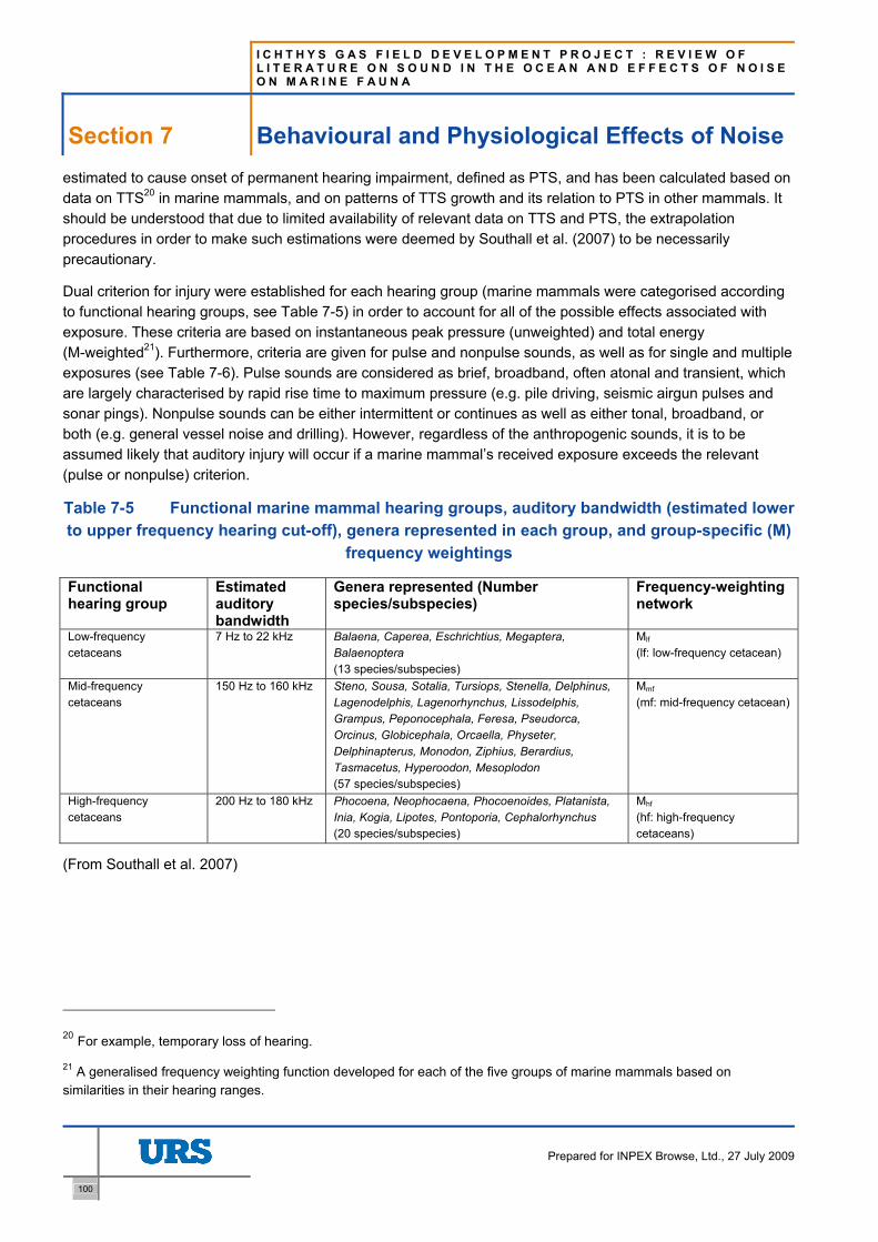
I C H T H Y S G A S F I E L D D E V E L O P M E N T P R O J E C T : R E V I E W O F L I T E R A T U R E O N S O U N D I N T H E O C E A N A N D E F F E C T S O F N O I S E O N M A R I N E F A U N A
Section 7 Behavioural and Physiological Effects of Noise
100
Prepared for INPEX Browse, Ltd., 27 July 2009
estimated to cause onset of permanent hearing impairment, defined as PTS, and has been calculated based on data on TTS20 in marine mammals, and on patterns of TTS growth and its relation to PTS in other mammals. It should be understood that due to limited availability of relevant data on TTS and PTS, the extrapolation procedures in order to make such estimations were deemed by Southall et al. (2007) to be necessarily precautionary.
Dual criterion for injury were established for each hearing group (marine mammals were categorised according to functional hearing groups, see Table 7-5) in order to account for all of the possible effects associated with exposure. These criteria are based on instantaneous peak pressure (unweighted) and total energy (M-weighted21). Furthermore, criteria are given for pulse and nonpulse sounds, as well as for single and multiple exposures (see Table 7-6). Pulse sounds are considered as brief, broadband, often atonal and transient, which are largely characterised by rapid rise time to maximum pressure (e.g. pile driving, seismic airgun pulses and sonar pings). Nonpulse sounds can be either intermittent or continues as well as either tonal, broadband, or both (e.g. general vessel noise and drilling). However, regardless of the anthropogenic sounds, it is to be assumed likely that auditory injury will occur if a marine mammal’s received exposure exceeds the relevant (pulse or nonpulse) criterion.
Table 7-5 Functional marine mammal hearing groups, auditory bandwidth (estimated lower to upper frequency hearing cut-off), genera represented in each group, and group-specific (M)
frequency weightings
Functional hearing group
Estimated auditory bandwidth
Genera represented (Number species/subspecies)
Frequency-weighting network
Low-frequency cetaceans
7 Hz to 22 kHz Balaena, Caperea, Eschrichtius, Megaptera, Balaenoptera (13 species/subspecies)
Mlf (lf: low-frequency cetacean)
Mid-frequency cetaceans
150 Hz to 160 kHz Steno, Sousa, Sotalia, Tursiops, Stenella, Delphinus, Lagenodelphis, Lagenorhynchus, Lissodelphis, Grampus, Peponocephala, Feresa, Pseudorca, Orcinus, Globicephala, Orcaella, Physeter, Delphinapterus, Monodon, Ziphius, Berardius, Tasmacetus, Hyperoodon, Mesoplodon (57 species/subspecies)
Mmf (mf: mid-frequency cetacean)
High-frequency cetaceans
200 Hz to 180 kHz Phocoena, Neophocaena, Phocoenoides, Platanista, Inia, Kogia, Lipotes, Pontoporia, Cephalorhynchus (20 species/subspecies)
Mhf (hf: high-frequency cetaceans)
(From Southall et al. 2007)
20 For example, temporary loss of hearing.
21 A generalised frequency weighting function developed for each of the five groups of marine mammals based on similarities in their hearing ranges.
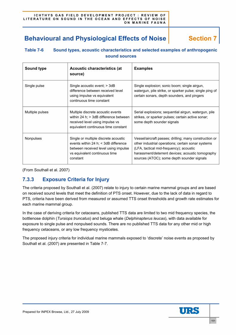
I C H T H Y S G A S F I E L D D E V E L O P M E N T P R O J E C T : R E V I E W O F L I T E R A T U R E O N S O U N D I N T H E O C E A N A N D E F F E C T S O F N O I S E
O N M A R I N E F A U N A
Behavioural and Physiological Effects of Noise Section 7
Prepared for INPEX Browse, Ltd., 27 July 2009
101
Table 7-6 Sound types, acoustic characteristics and selected examples of anthropogenic sound sources
Sound type Acoustic characteristics (at source)
Examples
Single pulse Single acoustic event; > 3dB difference between received level using impulse vs equivalent continuous time constant
Single explosion; sonic boom; single airgun, watergun, pile strike, or sparker pulse; single ping of certain sonars, depth sounders, and pingers
Multiple pulses Multiple discrete acoustic events within 24 h; > 3dB difference between received level using impulse vs equivalent continuous time constant
Serial explosions; sequential airgun, watergun, pile strikes, or sparker pulses; certain active sonar; some depth sounder signals
Nonpulses Single or multiple discrete acoustic events within 24 h; < 3dB difference between received level using impulse vs equivalent continuous time constant
Vessel/aircraft passes; drilling; many construction or other industrial operations; certain sonar systems (LFA, tactical mid-frequency); acoustic harassment/deterrent devices; acoustic tomography sources (ATOC); some depth sounder signals
(From Southall et al. 2007)
7.3.3 Exposure Criteria for Injury The criteria proposed by Southall et al. (2007) relate to injury to certain marine mammal groups and are based on received sound levels that meet the definition of PTS onset. However, due to the lack of data in regard to PTS, criteria have been derived from measured or assumed TTS onset thresholds and growth rate estimates for each marine mammal group.
In the case of deriving criteria for cetaceans, published TTS data are limited to two mid frequency species, the bottlenose dolphin (Tursiops truncatus) and beluga whale (Delphinapterus leucas), with data available for exposure to single pulse and nonpulsed sounds. There are no published TTS data for any other mid or high frequency cetaceans, or any low frequency mysticetes.
The proposed injury criteria for individual marine mammals exposed to ‘discrete’ noise events as proposed by Southall et al. (2007) are presented in Table 7-7.

I C H T H Y S G A S F I E L D D E V E L O P M E N T P R O J E C T : R E V I E W O F L I T E R A T U R E O N S O U N D I N T H E O C E A N A N D E F F E C T S O F N O I S E O N M A R I N E F A U N A
Section 7 Behavioural and Physiological Effects of Noise
102
Prepared for INPEX Browse, Ltd., 27 July 2009
Table 7-7 Proposed injury criteria for individual marine mammals exposed to 'discrete' noise events, either single or multiple exposures within a 24-h period
Marine Mammal Group Single pulses Multiple pulses Nonpulses
Low-frequency cetaceans
Sound pressure level 230 dB re: 1 μPa (peak) (flat) 230 dB re: 1 μPa (peak) (flat) 230 dB re: 1 μPa (peak) (flat)
Sound exposure level 198 dB re: 1 μPa2-s (Mlf) 198 dB re: 1 μPa2-s (Mlf) 215 dB re: 1 μPa2-s (Mlf)
Mid-frequency cetaceans
Sound pressure level 230 dB re: 1 μPa (peak) (flat) 230 dB re: 1 μPa (peak) (flat) 230 dB re: 1 μPa (peak) (flat)
Sound exposure level 198 dB re: 1 μPa2-s (Mmf) 198 dB re: 1 μPa2-s (Mmf) 215 dB re: 1 μPa2-s (Mmf)
High-frequency cetaceans
Sound pressure level 230 dB re: 1 μPa (peak) (flat) 230 dB re: 1 μPa (peak) (flat) 230 dB re: 1 μPa (peak) (flat)
Sound exposure level 198 dB re: 1 μPa2-s (Mhf) 198 dB re: 1 μPa2-s (Mhf) 215 dB re: 1 μPa2-s (M hf)
Note: Criteria in the “Sound pressure level” lines are based on the peak pressure known or assumed to elicit TTS-onset, plus 6 dB. Criteria in the “Sound exposure level” lines are based on the SEL eliciting TTS-onset plus (1) 15 dB for any type of marine mammal exposed to single or multiple pulses, (2) 20 dB for cetaceans in water exposed to nonpulses.
(From Southall et al. 2007)
7.3.4 Exposure Criteria for Behaviour It is noted that a key challenge in the development of behavioural criteria is being able to distinguish a significant behavioural response from an insignificant, momentary alteration in behaviour. To assess and quantify significant behavioural effects to noise exposure it is necessary to understand the impact such changes might have on critical biological changes, including growth, survival and reproduction.
It is noted by Southall et al. (2007) that most behavioural response studies to date have focused on short term and localised behavioural changes whose relevance to individual effects, let alone population factors, is considered low. As an example, it is believed unlikely that a startle response to a brief, transient event would persist long enough to create any response which could be deemed significant. In addition, even strong behavioural responses to single pulses would be expected to dissipate rapidly enough as to have limited long term effect on individuals, let alone populations.
In respect of behavioural responses to sound exposure, it is also evident that many more factors affect behaviour then just simple acoustic metrics. These include animal activity at the time of exposure, habituation and sensitisation to the sound, as well as the presence or absence of acoustic similarities between the

I C H T H Y S G A S F I E L D D E V E L O P M E N T P R O J E C T : R E V I E W O F L I T E R A T U R E O N S O U N D I N T H E O C E A N A N D E F F E C T S O F N O I S E
O N M A R I N E F A U N A
Behavioural and Physiological Effects of Noise Section 7
Prepared for INPEX Browse, Ltd., 27 July 2009
103
anthropogenic sound and biologically relevant signals in the animal’s environment (e.g. calls of conspecifics, predators or prey).
When considering information regarding behavioural responses, it is also worth considering information presented by Wartzok and Tyack (2007), who have elaborated on the Population Consequences of Acoustic Disturbance (PCAD) Model developed by the US National Research Council (comprised of 70 individuals). Wartzok and Tyack (2007) supported the findings of Southall et al. (2007) and reported that behavioural dose-response variability is greater than physiological dose response variability. In addition, they report that behavioural variability can also be dependent on age, sex, reproductive status, time of year and behavioural state.
Single Pulses
Noting the lack of available data for behavioural thresholds, Southall et al. (2007) propose that following exposure to a single pulse, significant behavioural disturbance should be considered to occur at the lowest level of noise exposure that has a measurable transient effect on hearing (i.e. TTS onset). It is recognised that TTS is not technically a behavioural effect, but is used because it’s believed that any compromise to hearing functions, even if it is temporary, has the potential to affect vital rates and therefore behaviour.
The recommended behavioural disturbance criteria for all cetaceans exposed to single pulses have been developed based on the results for TTS onset in a beluga whale exposed to a single pulse. Proposed unweighted peak sound pressure criteria have been set at 224 dB (re 1 µPa). The weighted sound exposure level22 criteria for mid frequency cetaceans have been set at 183 dB (re 1 µPa2-s). Through extrapolation the same criteria have also been set for low and high frequency cetaceans, the only difference being the influence of the respective frequency weighting functions for sound exposure criteria (see Southall et al. (2007) Chapter 3, pg 439).
Multiple Pulses and Nonpulses
In the case of multiple pulses and nonpulses, Southall et al. (2007) report that it is not currently possible to derive explicit criteria for behavioural disturbance. This conclusion is based on the large degree of variability in responses between groups, species and individuals. However, it is highlighted that most research in respect of low frequency cetaceans and nonpulses indicates no or very limited responses at a received level range of 90 to 120 dB (re 1 µPa) and an increasing probability of avoidance and other behavioural effects, albeit generally minor, at a range of 120 to 160 dB (re 1 µPa).
In the absence of data necessary to develop behavioural based criteria, Southall et al. (2007) undertook a severity scaling analysis of available observational data. This analysis was undertaken for the three cetacean groups, and includes a list of response scores from 0 to 9 with a corresponding behavioural reaction for each score (see Table 7-8). These scores are based on either individual and/or independent group behaviour.
22 Sound exposure level is a measure of energy. Specifically, it is the dB level of the time integral of the squared-instantaneous sound pressure normalised to a one second (1-s) period. It is useful in assessing cumulative exposure because it enables sounds of differing duration to be compared in terms of total energy (Southall et al. 2007).
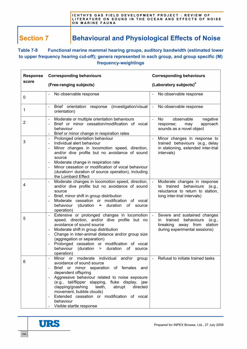
I C H T H Y S G A S F I E L D D E V E L O P M E N T P R O J E C T : R E V I E W O F L I T E R A T U R E O N S O U N D I N T H E O C E A N A N D E F F E C T S O F N O I S E O N M A R I N E F A U N A
Section 7 Behavioural and Physiological Effects of Noise
104
Prepared for INPEX Browse, Ltd., 27 July 2009
Table 7-8 Functional marine mammal hearing groups, auditory bandwidth (estimated lower to upper frequency hearing cut-off); genera represented in each group, and group specific (M)
frequency-weightings
Response score
Corresponding behaviours
(Free-ranging subjects)
Corresponding behaviours
(Laboratory subjects)ii
0 - No observable response - No observable response
1 - Brief orientation response (investigation/visual
orientation) - No observable response
2 - Moderate or multiple orientation behaviours - Brief or minor cessation/modification of vocal
behaviour - Brief or minor change in respiration rates
- No observable negative response; may approach sounds as a novel object
3 - Prolonged orientation behaviour - Individual alert behaviour - Minor changes in locomotion speed, direction,
and/or dive profile but no avoidance of sound source
- Moderate change in respiration rate - Minor cessation or modification of vocal behaviour
(duration< duration of source operation), including the Lombard Effect
- Minor changes in response to trained behaviours (e.g., delay in stationing, extended inter-trial intervals)
4 - Moderate changes in locomotion speed, direction,
and/or dive profile but no avoidance of sound source
- Brief, minor shift in group distribution - Moderate cessation or modification of vocal
behaviour (duration ≈ duration of source operation)
- Moderate changes in response to trained behaviours (e.g., reluctance to return to station, long inter-trial intervals)
5 - Extensive or prolonged changes in locomotion
speed, direction, and/or dive profile but no avoidance of sound source
- Moderate shift in group distribution - Change in inter-animal distance and/or group size
(aggregation or separation) - Prolonged cessation or modification of vocal
behaviour (duration > duration of source operation)
- Severe and sustained changes in trained behaviours (e.g., breaking away from station during experimental sessions)
6 - Minor or moderate individual and/or group
avoidance of sound source - Brief or minor separation of females and
dependent offspring - Aggressive behaviour related to noise exposure
(e.g., tail/flipper slapping, fluke display, jaw clapping/gnashing teeth, abrupt directed movement, bubble clouds)
- Extended cessation or modification of vocal behaviour
- Visible startle response
- Refusal to initiate trained tasks

I C H T H Y S G A S F I E L D D E V E L O P M E N T P R O J E C T : R E V I E W O F L I T E R A T U R E O N S O U N D I N T H E O C E A N A N D E F F E C T S O F N O I S E
O N M A R I N E F A U N A
Behavioural and Physiological Effects of Noise Section 7
Prepared for INPEX Browse, Ltd., 27 July 2009
105
Response score
Corresponding behaviours
(Free-ranging subjects)
Corresponding behaviours
(Laboratory subjects)ii
- Brief cessation of reproductive behaviour
7 - Extensive or prolonged aggressive behaviour - Moderate separation of females and dependent
offspring - Clear anti-predator response - Severe and/or sustained avoidance of sound
source - Moderate cessation of reproductive behaviour
- Avoidance of experimental situation or retreat to refuge area (> duration of experiment)
- Threatening or attacking the sound source
8 - Obvious aversion and/or progressive sensitization - Prolonged or significant separation of females and
dependent offspring with disruption of acoustic reunion mechanisms
- Long-term avoidance of area (> source operation) - Prolonged cessation of reproductive behaviour
- Avoidance of or sensitization to experimental situation or retreat to refuge area (> duration of experiment)
9 - Outright panic, flight, stampede, attack of
conspecifics, or stranding events - Avoidance behaviour related to predator detection
- Total avoidance of sound exposure area and refusal to perform trained behaviours for greater than a day
(From Southall et al. 2007)
It should be noted that in the context of behavioural responses in respect to the assessment of risk from noise, a response score of 0 to 6 would in most occurrences be considered a minor or transitory impact, while a score of 8 to 9 would most likely be considered significant, as it is likely to affect vital rates. A score of 7 would represent the threshold of onset of significant behavioural response.
The PCAD model (see Figure 7-4) was developed as framework to describe and assess acoustic stimuli in relation to population level effects. It is a first attempt at tracing acoustic disturbance through the entire life history of a marine mammal and determining the final consequences for a population (NRC, 2005).
The PCAD model requires an understanding of normal behaviour and use of sound and involves five different variables (sound, behaviour change, life function, vital rate and population effect) that are linked by four transfer steps. The first step relates the acoustic source to a behavioural response. The second defines the behavioural disruption in terms of potential effects on critical life functions (e.g. feeding and breeding). The third step aims to integrate these functional outcomes of responses over daily and seasonal cycles, and link them to vital rates in life history. The final step then relates the changes in vital rates of individual animals to overall population effects. However, it should be noted that the PCAD model is intended to serve as a conceptual model only (NRC 2005).
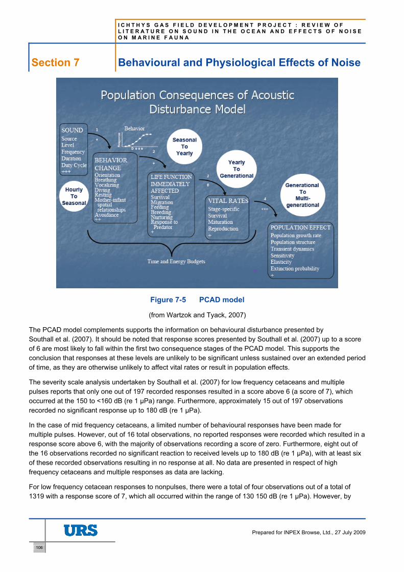
I C H T H Y S G A S F I E L D D E V E L O P M E N T P R O J E C T : R E V I E W O F L I T E R A T U R E O N S O U N D I N T H E O C E A N A N D E F F E C T S O F N O I S E O N M A R I N E F A U N A
Section 7 Behavioural and Physiological Effects of Noise
106
Prepared for INPEX Browse, Ltd., 27 July 2009
Figure 7-5 PCAD model
(from Wartzok and Tyack, 2007)
The PCAD model complements supports the information on behavioural disturbance presented by Southall et al. (2007). It should be noted that response scores presented by Southall et al. (2007) up to a score of 6 are most likely to fall within the first two consequence stages of the PCAD model. This supports the conclusion that responses at these levels are unlikely to be significant unless sustained over an extended period of time, as they are otherwise unlikely to affect vital rates or result in population effects.
The severity scale analysis undertaken by Southall et al. (2007) for low frequency cetaceans and multiple pulses reports that only one out of 197 recorded responses resulted in a score above 6 (a score of 7), which occurred at the 150 to <160 dB (re 1 µPa) range. Furthermore, approximately 15 out of 197 observations recorded no significant response up to 180 dB (re 1 µPa).
In the case of mid frequency cetaceans, a limited number of behavioural responses have been made for multiple pulses. However, out of 16 total observations, no reported responses were recorded which resulted in a response score above 6, with the majority of observations recording a score of zero. Furthermore, eight out of the 16 observations recorded no significant reaction to received levels up to 180 dB (re 1 µPa), with at least six of these recorded observations resulting in no response at all. No data are presented in respect of high frequency cetaceans and multiple responses as data are lacking.
For low frequency cetacean responses to nonpulses, there were a total of four observations out of a total of 1319 with a response score of 7, which all occurred within the range of 130 150 dB (re 1 µPa). However, by

I C H T H Y S G A S F I E L D D E V E L O P M E N T P R O J E C T : R E V I E W O F L I T E R A T U R E O N S O U N D I N T H E O C E A N A N D E F F E C T S O F N O I S E
O N M A R I N E F A U N A
Behavioural and Physiological Effects of Noise Section 7
Prepared for INPEX Browse, Ltd., 27 July 2009
107
comparison, over 1300 other observations at these levels received a score of 6 or less. There were no observational data available for any animal exposed to received levels greater then 150 dB (re 1 µPa).
In the case of mid frequency cetaceans exposed to nonpulses, some field studies showed high severity scores to exposures from 90 to 100 dB (re 1 µPa), while others failed to exhibit responses to exposures up to 170 dB (re 1 µPa). In some controlled studies exposing bottlenose dolphins to received levels at up to 200 dB some observations displayed no discernable response, while an equal number of observations recorded a response level of 8. It is believed that contextual variables other than received levels, as well as species differences, are the likely reasons for this variability. It is also noted that exposures within captive settings generally exceeded 170 dB (re 1 µPa) before a response was recorded.
Out of the 214 observations of mid frequency cetaceans exposed to nonpulses, 20 recorded a response score of 8. Of these 20 observations, 14 were at received levels of 90 to 150 dB (re 1 µPa), with eight of these observations made at received levels between 90 to 110 dB (re 1 µPa) (although these observations involved relatively quiet Arctic waters). By way of contrast, 194 other observations were made at levels up to 200 dB (re 1 µPa), with no significant response recorded.
For high frequency cetaceans exposed to nonpulses, 109 observations were made at received levels up to 170 dB, none of which recorded a response score above 6.
When considering the observational data described above, Southall et al. (2007) identified some behavioural responses at their ascribed levels of 7 or above (considered and described as acute effects). However, when placed in the context of the PCAD model, any anthropogenic noise impact, especially at the level of around 6 to 7, would need to exert a chronic (or sustained) ongoing influence at this level to begin manifesting as population level effects.
7.3.5 Conclusion It is recognised that the work by Southall et al. (2007) has resulted in some advance in the empirical understanding of underwater anthropogenic noise and potential impacts on marine mammals, particularly in respect of providing an up-to-date review of available literature and the derivation of quantitative criteria for auditory injury to marine mammals. However, it is acknowledged that further information and research is required. For example, it is widely accepted that it’s not possible to propose any meaningful criteria in respect of behavioural disturbance due to the lack of information and studies relating to noise and behavioural effects. How these behavioural effects then may impact upon populations is also unknown. This is largely due to the limited amount of data, limited species information and the dearth of contextual information regarding the influences of factors such as duration, habituation and the ambient noise environment etc.
The need for extrapolation and precautionary assumption by Southall et al. (2007) to develop their criteria highlights the need for research in a variety of areas. Noting this, it is important that the information presented by Southall et al. (2007) is not considered definitive. In many cases the proposed criteria for an entire marine mammal group are based on precautionary results for a species within that group, even though anecdotal and some other empirical data exist which show higher exposures are required to induce the same event in other circumstances. Similarly, care must be exercised when considering the information presented on behavioural effects, as the recorded observations are limited to a small number of species and only certain received sound levels.

I C H T H Y S G A S F I E L D D E V E L O P M E N T P R O J E C T : R E V I E W O F L I T E R A T U R E O N S O U N D I N T H E O C E A N A N D E F F E C T S O F N O I S E
O N M A R I N E F A U N A
Effects of Noise on Marine Fauna Section 8
Prepared for INPEX Browse, Ltd., 27 July 2009
109
8 Effects of Noise on Marine Fauna
This section reviews the known effects on important marine fauna from likely noise sources associated with the Project. It reports on recorded observations and analyses from around the globe and does not specifically focus upon Darwin, the Browse Basin or Australia in general, but is rather intended to provide a general background to the literature on the effects of anthropogenic noise upon sensitive or charismatic marine fauna.
It is difficult to predict which species will be most vulnerable to man made noise because of the wide range of individual and population sensitivities as well as differences in wariness or motivation or degree of habituation. Currently, it may only be possible to make generalisations about the vulnerability of species groups based on behavioural observations of responses to man made sounds, habits and what is known about a species’ auditory sensitivity or vocal range.
When evaluating likely impacts, consideration should also be given to differences in local conditions that may affect sound propagation, e.g. depth, bottom type, size and type of source. A majority of man-made sounds have significant amounts of energy at low frequencies, thereby leading to potential disturbance, damage or interference to the mysticete whales. There is evidence of low frequency hearing in sperm whales (Ketten 1992, 1997) and this species appears to be extremely sensitive to disturbance from a variety of sound sources. Deep diving odontocetes may also be at risk of exposure as their behaviour puts them in the deep sound channel or Sound Fixing and Ranging (SOFAR) channel, along which sound can travel efficiently for distances of hundreds to thousands of kilometres, but this is only of any possible relevance for deeper, offshore locations.
The sources of noise which will be examined include dredging, pile driving, shipping noise and vessel presence, rock dumping and dredge spoil disposal, seismic surveys, drilling, underwater blasting and pipelaying and operation.
8.1 Dredging Reported source levels for general marine dredging operations range from 160 to 180 dB (re 1 µPa @ 1 m) for 1/3 octave bands with peak intensity between 50 and 500 Hz (Greene and Moore 1995). One of the most comprehensive studies of underwater noise emissions from dredging was carried out by the United States Army Corps of Engineers in Cook Inlet, Alaska (Dickerson et. al. 2001). The research provides detailed records of the underwater noise generated by a bucket (grab) dredging operation. Measurements of the dredging in Cook Inlet, showed that the bucket striking coarse gravels on the seabed generated the most noise with a recorded peak of 124 dB (re 1 µPa) at 150 m from the dredge site which attenuated by 30 dB (re 1 µPa) over a distance of 5 km. The digging operation was characterised by a grinding noise with a recorded peak of 113.2 dB (re 1 µPa) at 150 m from the dredging site to 95 dB (re 1 µPa) 5 km away.
Recorded noise levels for large cutter suction dredgers are higher than those associated with grab dredgers. Recorded broadband noise data for the large cutter suction dredger JFJ de Nul are given as 183 dB (re 1 µPa at 1 m) at Sakhalin Island, 2004. Measurements of two suction dredgers, Aquarius and Beaver Mackenzie, are reported in Nedwell and Howell (2004). Their octave band spectra peak between 80 and 200 Hz, with Aquarius having the higher of the two spectra peaking at approximately 177 dB (re 1 µPa at 1 m). In the 20-1000 Hz band, Beaver Mackenzie and the Aquarius were measured to have a 133 dB (re 1 µPa) level at 0.19 km and a 140 dB (re 1 µPa) level at 0.2 km, respectively.
Information from a number of conservative studies indicates that acute damage to fish caused by sound does not occur below about 160 dB (re 1 µPa). During grab dredging activities, this noise level is unlikely to be generated, even when dredging through partially consolidated rock. However, noise levels as high as, or higher

I C H T H Y S G A S F I E L D D E V E L O P M E N T P R O J E C T : R E V I E W O F L I T E R A T U R E O N S O U N D I N T H E O C E A N A N D E F F E C T S O F N O I S E O N M A R I N E F A U N A
Section 8 Effects of Noise on Marine Fauna
110
Prepared for INPEX Browse, Ltd., 27 July 2009
than, 160 dB (re 1 µPa) could be generated in close proximity to the cutter suction dredger. This indicates that any potential for acute damage to fish would only be likely to occur in very close proximity to the cutter head.
Thus, at distances greater than 10s of metres at most, acute damage would not be likely to occur. Fish may avoid moving close to a working dredger head as the sound may cause an avoidance response, and therefore acute damage would only occur if fish were present in the vicinity when dredging operations started. This in itself may be unlikely given the physical disturbance that this activity will cause.
It has also been calculated that the majority of fish would not be able to detect the noise made by dredging activity at a distance greater than 1 km from the activity. Henderson (2003), assuming spherical spreading of sound, calculated that the predicted sound level from a cutter suction dredger would be 100 dB (re 1 µPa) at 1 km. On this basis it is considered that the noise generated during dredging would not lead to fish mortality and at worse would lead to temporary avoidance of nearshore waters immediately adjacent to the dredging activity.
Dredging noise varies through time and periodically dredging ceases whilst the dredger spuds in or undertakes maintenance and repair. This creates periods of calm and quiet, during which fish can move through the area undisturbed.
8.2 Pile Driving The intense pulses of pile driving have been observed to injure swim bladders and kill salmonid fishes in limited circumstances, and they have the potential to elicit a startle response to cetaceans, particularly if the hammering operation is commenced without any form of soft-start procedure. A ‘worst case’ scenario in terms of invoking undue stress to whales would involve start up of a three month operation at a site located in a shallow embayment that is being used for calving or resting, or as a temporary stop-over by humpback cow calf pairs.
An assessment of the effect of impact pile driving noise on fish species predominant near Rødsand, Denmark was made by Engell-Sørensen (2000). This work assessed the potential behavioural and physical effects of the noise levels of pile driving associated with construction of offshore wind turbines. Sound Exposure Levels for four measurement positions between 30 to 720 m from the activity gave levels ranging from 166 dB to 188 dB (re 1 µPa), with a calculated Source Level of 210 dB (re 1 μPa at 1 m). Engell-Sørensen (2000) concluded that: avoidance reactions would be likely to occur up to 30 m from the source, especially for species with swim bladders; the measured noise levels could harm the hearing ability of clupeids such as herring (Clupea harengus) and sprat (Sprattus sprattus), but this may regenerate over time; and, other than those already mentioned, the noise from pile driving is unlikely to cause any other physical effect.
From their review of the available literature, Popper et al. (2006) propose interim criteria for injury to fish exposed to pile driving activities. As described in Section 7.1.6, Popper et al. (2006) suggest dual criteria, and propose that the onset of direct physical injury to fish exposed to pile driving would be at a sound exposure level of 187 dB (re 1 µPa2.sec) and a peak sound pressure level of 208 dB (re 1 µPapeak).These criteria are in line with the findings of Caltrans (2004) (cited in Popper et al. 2006), which showed no damage to steelhead (Oncorhynchus mykiss) and shiner surfperch23 (Cymatogaster aggregata) when exposed to sound levels of between 158-182 dB (re 1 µPa2.sec) at distances of 23 m to 316 m, and peak levels within the same range.
23 Note both these fish are teleost species, as are Barramundi, and would be expected to exhibit similar hearing acuity.
I C H T H Y S G A S F I E L D D E V E L O P M E N T P R O J E C T : R E V I E W O F L I T E R A T U R E O N S O U N D I N T H E O C E A N A N D E F F E C T S O F N O I S E
O N M A R I N E F A U N A
Effects of Noise on Marine Fauna Section 8
Prepared for INPEX Browse, Ltd., 27 July 2009
111
8.3 Shipping Noise It is widely considered that the baleen whales have evolved their low frequency vocalisations as a result of selective advantages of achieving long distance communications, with the largest species most capable of exploiting the ocean's natural sound ducts. The apparent ‘male only’ intense calling behaviour now known for the three blue whales plus the fin and humpback whales implies a reproductive strategy. If only the males make the loudest, longest and most complex calls among the range of vocalisations emitted by both sexes, these may help females select fit males to help ensure successful calving and genetic quality of their progeny. In this context, Croll et al. (2002) speculated that if breeding is “limited by the encounter rate of receptive females with singing males, the recovery of fin and blue whale populations from past exploitation could be impeded by low frequency sounds generated by human activity”. If it is accepted that the two sexes possess no other mechanisms for (a) navigating to their usual breeding area during the same season, and (b) undertaking relatively simple random-search strategies to yield audible range encounters (e.g. 50-100 km wide cross tracks), this concept increases the impact significance of potential call-masking sound sources (i.e. a breeding area where low frequency background noise is continuously elevated by heavy shipping traffic).
In the case of the potential for shipping or other low frequency sources to mask the long distance calls of baleen whales in Australian waters, there are few locations where ambient noise is significantly elevated by heavy shipping traffic (see Section 5 2) and there are no concentrated offshore petroleum developments where supply vessels, rig tenders and oil tankers are sufficiently numerous to contribute markedly to regional ambient noise, as can occasionally occur in parts of the North Sea, north east Atlantic and Gulf of Mexico 24 .
In this context, McCauley and Cato (2003) have criticised Andrew et al. (2002) who claimed, from a comparison of records from an established deep sound channel acoustic monitoring system off Point Sur (north California), that current ambient noise levels in the North Pacific had increased in selected low frequency bands (20-80 Hz and 200-300 Hz) compared to levels measured from the same equipment in the 1960s, offering support to the concept that rising vessel traffic noise is significantly limiting communications between baleen species which produce sounds at the same frequencies (Payne & Webb 1971). McCauley and Cato (2003) considered that the records comparison by Andrew et al. (2002) was marred by a recent calibration of the Point Sur equipment, by the dismissal in their calculations of the contribution of distant great whale calling, and that traffic noise reference levels were based on limited knowledge from 30-35 year old samples. Great whale numbers in the Pacific during the 1960s were historically at their lowest levels due to commercial whaling and hence would have contributed little to the low frequency components of ambient noise. Recoveries in their numbers over the recent decades mean that great whales calling from thousands of kilometres away could well be adding to the ambient noise in the deep sound channel where the Point Sur measurements are made.
Arguments that shipping traffic noise is significantly masking great whale communications in all regions also assume that the northern hemisphere, with its high density of busy shipping lanes, is typical of all oceans and seas including those in the southern hemisphere (McCauley & Cato 2003). Yet even in the high traffic areas of the Tasman Sea, wind-induced sea surface noise drowns out shipping noise whenever wind speeds attain
24 The north west Atlantic, west Shetland area and parts of the Mediterranean represent regions where limited rorqual stocks and such activities overlap, and the potential for excessive background noise in these areas to affect the recovery of northern fin and blue whale stocks has been raised by some workers such as Croll et al. (2001).

I C H T H Y S G A S F I E L D D E V E L O P M E N T P R O J E C T : R E V I E W O F L I T E R A T U R E O N S O U N D I N T H E O C E A N A N D E F F E C T S O F N O I S E O N M A R I N E F A U N A
Section 8 Effects of Noise on Marine Fauna
112
Prepared for INPEX Browse, Ltd., 27 July 2009
20 knots or more (see Figure 4-2). McCauley and Cato (2003) have also noted that whales have always had to contend with noise levels that are as high as, or higher than, ship traffic noise, and that in some areas their own calls are producing greater ambient noise levels than traffic noise when averaged over time.
In another study, shipping noise levels were examined with respect to resident sperm whales feeding in the Canary Islands (André & Degollada, 2003). This study was undertaken following fears that the sperm whales, which are exposed to heavy ferry and merchant ship traffic, were suffering increased collision rates due to adverse effects from the local acoustic budget. However controlled exposure experiments to test the ability of underwater sound system to repel sperm whales from ferry routes and thus reduce collision risks found that none of the low frequency sounds tested altered their behaviour or location. This is perhaps unsurprising given the apparent disdain displayed to merchant ships by sperm whale groups when feeding and surface resting in the busy shipping lane off Sri Lanka. In a recent (May 2003) example of this behaviour, a family group of 40-50 sperm whales were monitored for some 12 hours while feeding and socialising in the busy shipping lane 50 miles south of Dondra Head (south Sri Lanka). “Numerous tankers” were passing during this period since the whales were inside the very busy oil tanker and container ship lane between Asia and the Gulf and Suez Canal, and it was speculated that the whales had been attracted to an area containing abundant prey (Madsen 2003). During the observations, a subgroup of 10 were observed to show no apparent change in their surface resting behaviour and slow swimming speed as a large, fast-moving container ship passed just behind their own surface wake.
Erbe (2002) modelled the potential effects of underwater noise from whale-watching vessels on orcas off southern Canada. Results indicated that faster boats made more noise, being audible to killer whales over 16 km away, to mask killer whale calls over 14 km, to elicit behavioural response over 200 m and to cause changes in hearing of 5 dB after 30 minutes within 450 m. For slower vessel speeds the predicted ranges were 1 km for audibility and masking, 50 m for behavioural responses, and 20 m for hearing changes. The effects of combined vessel noise around a group were close to a level considered likely to cause a permanent hearing loss if there was prolonged exposure.
Concerns about long distance masking would require a major rise in shipping traffic, discovery of offshore oil reservoirs on a par with the size of those off Scotland or Norway, or a major new industrial port complex proposed near a recognised significant baleen whale locality. In this context, experience from the right, humpback and sperm whale stocks in the North Atlantic and Mediterranean indicates that increased rates of ship strikes rather than call masking would be a more plausible concern regarding the ability of vessel traffic to influence population recovery rates.
A considerable body of fisheries literature exists on the behavioural response of fish to the noise of approaching vessels (e.g. Olsen 1990). These studies have shown that fish avoid approaching vessels when the radiated noise levels exceed their threshold of hearing by 30 dB or more, usually by swimming down or horizontally away from the vessel path. Environmental and physiological factors play a part in determining the noise levels that will trigger an avoidance reaction in fish. For many vessels fish avoidance reaction distances are 100-200 m but for the noisiest 400 m is more likely. The degree of observed effect weakens with depth, with fish below about 200 m depth being only mildly affected and the effect is only temporary with normally schooling patterns resuming shortly after the noise source has passed. Surface and mid water dwelling fish may theoretically be adversely affected by noise generated during vessel movement, however the clear and abundant presence of fish that accumulate adjacent to operating industrial infrastructure (oil/gas production platforms, wharves, shiploaders, etc.) indicates that they are able to habituate to some noise with no apparent detriment.

I C H T H Y S G A S F I E L D D E V E L O P M E N T P R O J E C T : R E V I E W O F L I T E R A T U R E O N S O U N D I N T H E O C E A N A N D E F F E C T S O F N O I S E
O N M A R I N E F A U N A
Effects of Noise on Marine Fauna Section 8
Prepared for INPEX Browse, Ltd., 27 July 2009
113
8.4 Vessel Presence Humpback whales have been reported to show various responses to moving sources such as whale-watching vessels, fishing boats and recreational craft (Beach & Weinrich 1989, Clapham et al. 1993, Atkins & Swartz 1989). The types of approach, avoidance and apparent non-responses in behaviour to vessels have been related to the type, number and activity of the whales at the time of the observed interactions (Herman et al. 1980, Watkins. 1981, Krieger & Wing 1986). In early research, some investigators suggested that vessel traffic would cause humpback whales to avoid or leave both winter feeding and summer calving areas (Jurasz & Jurasz 1979b), while subsequent researchers have noted evidence suggesting that humpback whales can habituate to vessel traffic but may become more vulnerable to ship strikes once habituated (Swingle et al. 1993; Wiley et al. 1995).
Humpback whales are occasionally killed by ship strikes along both US coasts. On the Pacific side a humpback whale is killed about every other year, while six out of 20 humpback whales stranded along the mid-Atlantic coast had evidence of a major ship strike. In Alaska, the number of cruise ships entering Glacier Bay has been limited to reduce their possible disturbance to feeding humpback whales. In Hawaii, regulations prohibit vessels including whale-watching boats from approaching within 91 m of humpback whales and within 274 m in areas designated additional protection to cow calf pairs.
In a long-term study over 25 years of whale responses to vessel approaches (Watkins 1986), the most vigorous responses by whales came from vessel noise sources that changed suddenly, rapidly, increased or were unexpected. Watkins was one of the first to recognise that preoccupied whales were typically less responsive than inactive whales. Later workers have found similar results where rapidly changing vessel noise often evokes a strong avoidance response, while a slow non-aggressive vessel approach results in little response from the whales, noting that feeding whales may be less responsive to vessel traffic as they are involved in a biologically important, directed activity (Richardson et al. 1995; McCauley et al. 1996).
Vessel activity has been implicated in long-term and short term changes in distribution of humpback whales in Hawaiian waters (Norris & Reeves 1978, Jurasz & Palmer 1981, Baker & Herman 1989). Results from a long term study (27+ years) of southern right whales in Argentina imply flexibility in several aspects of their habitat use (Rowntree et al. 2001). This included the apparent abandonment of one calving/resting ground and establishment of a new ‘nursery’ beside the centre of a growing whale-watching industry, plus some small-scale shifts in distribution possibly in response to natural and human disturbances.
While family groups of sperm whales can exhibit apparent en masse indifference to the relatively intense emissions of nearby large and fast-moving ships that maintain steady courses (e.g. Sri Lanka, Canary Islands), individual sperm whales in New Zealand’s famous nearshore feeding area off Kaikoura displayed individualistic, contrasting reactions to outboard-powered RHIBs used for commercial whale-watching, as studied in the early 1990s (Gordon et al. 1992). ‘Resident’ whales appeared more tolerant of these vessels but spent shorter surface intervals and a more erratic and overall lower number of ventilations when RHIBs were present. ‘Non-resident’ sperm whales were much less tolerant of RHIB approaches and also reduced their surface intervals and ventilations when one or more of these vessels were present in the area. Evidence for slightly slower rates of initial descent was apparent in the rates of change of the bouts of clicks following the start of a feeding dive (marked by a fluke-up). No change to vocalisation or fluke-up could be related to RHIB presence/absence (Gordon et al. 1992).
I C H T H Y S G A S F I E L D D E V E L O P M E N T P R O J E C T : R E V I E W O F L I T E R A T U R E O N S O U N D I N T H E O C E A N A N D E F F E C T S O F N O I S E O N M A R I N E F A U N A
Section 8 Effects of Noise on Marine Fauna
114
Prepared for INPEX Browse, Ltd., 27 July 2009
8.5 Rock Dumping and Dredge Spoil Disposal Rock dumping and dredge spoil disposal are likely to be intermittent during construction activities. Noise from rock dumping is likely to be broadband low frequency, although at relatively modest source levels. Potential effects upon marine fauna are therefore most likely to be limited to startle responses or temporary avoidance behaviour. The prevailing lack of any apparent literature presenting discussion or observations of the effects of rock dumping / dredge spoil disposal upon marine fauna supports this conclusion.
Rock dumping / dredge spoil disposal is not expected to generate noise to any appreciable extent, except for that generated by the vessels themselves.
8.6 Seismic Surveys 8.6.1 Vertical seismic profiling VSP is used to correlate the subsurface geological layers identified through pre-drilling seismic surveys with the subsurface geological layers identified through cuttings returns and other data (e.g. wireline logging data) acquired during the drilling process.
VSP produces significantly less energy compared to large scale offshore seismic surveys, and therefore potential effects upon marine fauna would be considered much lower then those for large surveys. As noted, offshore seismic surveys generally consist of multiple (up to 20) air guns operating at around 2000 psi and expelling a volume of air of 4000 cui. At the source, pulses are between 220–240 dB (re 1 μPa at 1m), with sound levels reducing to 170–180 dB within 1 km and approximately 150 dB within 10 km. This compares to VSP, which may use a two to three airgun cluster, with each airgun also operating at around 2000 psi, but only expelling a volume of approximately 150 cui, creating a far smaller pressure pulse. The airgun cluster will typically be fired at intervals of 6-10 seconds, generating a sound signal strength of approximately 190 dB (re 1 µPa at 1 m), with a frequency typically centred around 200 Hz.
Using the practical spreading law25, the received sound levels from an acoustic source generating 190 dB (re 1 µPa at 1 m) would attenuate at approximately the rate displayed in Table 8-1. Practical spreading is preferred when water depth in which VSP will be taking place is not quite deep enough for the spherical spreading laws to be used. Also, as seabed absorption has not been taken into consideration, the use of practical spreading therefore provides a conservative estimate of received levels at various distances from the acoustic source.
25 The practical spreading law is used as a convenient rule of thumb when acoustic propagation conditions are unknown. This law presents a rate of loss which is a hybrid of spherical spreading and cylindrical spreading according to the equation TL (dB re 1 m) = 15 log10 r, where TL represents transmission loss and r (range) is the horizontal distance between source and receiver (metres).

I C H T H Y S G A S F I E L D D E V E L O P M E N T P R O J E C T : R E V I E W O F L I T E R A T U R E O N S O U N D I N T H E O C E A N A N D E F F E C T S O F N O I S E
O N M A R I N E F A U N A
Effects of Noise on Marine Fauna Section 8
Prepared for INPEX Browse, Ltd., 27 July 2009
115
Table 8-1 Attenuation of acoustic signal from vertical seismic profiling
Drop in sound intensity (dB re 1 µPa)
Received sound level (dB re 1 µPa)
Approximate distance from source(m)
10 180 4.5
20 170 22
30 160 100
40 150 464
50 140 2000
Table 8-1 shows how the received sound levels from an acoustic source generating 190 dB (re 1 µPa at 1 m), will attenuate rapidly with increasing distance from the acoustic source.
8.7 Drilling As previously noted, drilling noise is generally low level, low frequency and continuous with most energy concentrated below 1 kHz. Since this is a level in which most toothed whales have reduced hearing sensitivity, only in rare circumstances would drilling affect these species (Bassett 2008). However, the susceptibility of baleen whale and sirenians to disturbance from drilling may be higher, particularly for baleen whales, as it is presumed their hearing sensitivity is higher at low frequencies. In rare circumstances, Evans and Nice (1996) reported continuous sound produced by drilling activities may elicit behavioural avoidance in baleen whales at received sound levels of 110 to 130 dB (re 1 μPa). McCauley et al. (2000) cited some evidence of avoidance behaviour in some circumstances at received levels in excess of 160 dB, but this was considered more likely to emanate from drill rig support vessels rather than the drill itself.
8.8 Explosives Blasting will most likely be undertaken using the “drill and blast” method, sometimes known as confined blasting. This method involves small holes being drilled within the rock with charges placed and connected in the holes for subsequent firing. Potential effects from the drill and blast method are likely to be less significant then those from surface blasting operations (e.g. charges placed directly on to the seabed/rock). This is primarily due to the fact that surface blasting requires a greater charge to break up the rock (generally three times greater than the drill and blast method), and the explosive energy is dispersed more evenly throughout the water column, rather then directly at the rock (Ecos, 1996). When the drill and blast method is employed, not only are fewer, smaller charges required, but the blast effect is significantly contained. This not only attenuates the blast effect expressed in the water column but also serves to limit the sharp pressure fluctuation associated with a blast impulse; it is this sharp raise and variation in pressure that is responsible for most physiological damage in the near field of a detonation. As such, many of the effects presented below, unless specifically referenced to confined blasting, could be considered to be less for confined blasting projects. This is supported by an estimated comparison of unconfined and confined blasting presented by Ecos (1996), as shown in Table 8-2 and 8-3.

I C H T H Y S G A S F I E L D D E V E L O P M E N T P R O J E C T : R E V I E W O F L I T E R A T U R E O N S O U N D I N T H E O C E A N A N D E F F E C T S O F N O I S E O N M A R I N E F A U N A
Section 8 Effects of Noise on Marine Fauna
116
Prepared for INPEX Browse, Ltd., 27 July 2009
Table 8-2 Peak pressure (kPa) at distance from underwater (surface) blast
Explosive Mass (kg) Distance from Target (m)
1 2 5 10 50 100 150 200
5 8858 11471 16143 20905 38098 49335 57387 63886
10 4047 5241 7376 9552 17407 22542 26221 29190 50 656 850 1196 1549 2824 3654 4254 4736
100 300 388 546 708 1290 1671 1943 2164
250 107 138 194 251 458 593 690 768
500 48 63 89 114 209 271 315 351
1000 22 28 41 52 96 123 144 160 2000 10 13 18 24 44 57 66 73
(from Ecos 1996)
Table 8-3 Peak pressure (kPa) at distance from underwater (confined) blast
Explosive Mass (kg) Distance from Target (m)
1 2 5 10 50 100 150 200
5 3543 4588 6457 8362 15239 19734 22955 25554 10 1619 2096 2951 3820 6963 9016 10489 11676 50 262 340 479 620 1130 1463 1702 1894 100 120 155 218 283 516 668 777 865 250 43 55 77 100 183 237 276 307 500 19 25 35 46 84 108 126 140 1000 9 11 16 21 38 50 58 64 2000 4 5 7 10 18 23 26 29
(from Ecos 1996)
Further amelioration of the potential adverse effects from explosive blasting is afforded when a detonation event is composed of a number of smaller, individual charges. The connecting fuses of explosives generate small but significant timing delays within a combined charge. Each detonation event therefore comprises a chain of individual subordinate detonations, and these produce irregular and less pronounced peak pressure levels than would occur if all the explosives could be detonated simultaneously, or if a single aggregate charge of the same net explosive content was detonated.
8.8.1 Marine Mammals Richardson et al. (1995) reported on observed effects of explosives upon the behaviour of marine mammals. Humpback whales in the vicinity of explosives being detonated near Bermuda displayed no interruption to their vocalisations. Similarly, humpbacks within 2 km of explosions in sub-bottom rocks off Newfoundland displayed
I C H T H Y S G A S F I E L D D E V E L O P M E N T P R O J E C T : R E V I E W O F L I T E R A T U R E O N S O U N D I N T H E O C E A N A N D E F F E C T S O F N O I S E
O N M A R I N E F A U N A
Effects of Noise on Marine Fauna Section 8
Prepared for INPEX Browse, Ltd., 27 July 2009
117
no obvious reactions when 200 to 2,000 kg charges were detonated. Gray whales within a ‘few’ kilometres of detonations of 9 to 36 kg charges used during seismic survey have been observed to alter swimming behaviour, while other observers (Fitch and Young 1948, in Richardson et al. 1995) report the whales “were seemingly unaffected and in fact were not even frightened from the area”.
Toothed whales show a tolerance for impulsive acoustic disturbances, although the initial reaction may be one of avoidance. Captive false killer whales showed no obvious reaction to small charges, and other odontocetes have been found to be attracted to the location of detonations (Richardson et al. 1995), presumably in search of dead, injured or disoriented fish as prey.
Risk of physical injury or mortality does exist for large fauna, but these are only realistic probabilities in the immediate zone around the point of detonation and only for charges substantially larger than those likely to be used for the Project; these risks are ameliorated by standard marine fauna observation and clearance procedures of no more than a few hundred metres (Lewis 1996a).
Although any use of explosives during construction of the Project will be detectable over a wide area by potentially sensitive fauna, this risk is considered minimal when it is noted that use of explosives will be confined, irregular, dispersed over time and intermittent. This conclusion is supported by Richardson et al. (1995), who summarised that while some odontocetes, in particular, display short-term avoidance reactions to explosive impulses, overall, marine mammals show considerable tolerance of noise pulses from explosions. This conclusion is supported by observed reactions to explosives used singly or repetitively. The observed tolerance of marine mammals may be linked to their experience of the intense, impulsive nature of many acoustic events of natural origin, such as lightning and whale breaching and tail slapping.
8.8.2 Fish Popper et al. (2006) report on the detailed review by Hastings and Popper (2005) for which they converted data collected by Yelverton et al. (1975) to sound exposure levels. This resulted in no injuries occurring from blasts to the smallest fish (0.01 g) at up to 193 dB (re 1µPa2.second).
Sharks may be less susceptible to blast and impulse effects than are many fish. This is due to the absence of a swim bladder, their physical size and arguably also due to their general morphology. While fish without swim bladders are much less sensitive to blast pressure damage than swim bladder fish, it is worthy of note that fish with a cylindrical body shape (e.g. barracuda, queenfish, kingfish) have been found less vulnerable than laterally compressed fish with thin-walled bladders (Lewis 1996a).
8.8.3 Marine Turtles In the case of shockwave effects, there are very little hard data available on the types and extent of turtle tissue damage due to underwater detonations, and most workers assume that turtle lungs, ear drums and other gas-containing organs would be affected to the same degree as their counterparts in marine mammals (Lewis 1996a).
Due to the lack of specific injury response curves for turtles, Young (1991) followed US National Marine Fisheries Service criteria for sea turtles in the Gulf of Mexico and provided safe distance ranges plots for sea turtles based on cube root scaling, where:
Turtle Safe Range (feet) = 560 x NEQ TNT (lbs)1/3

I C H T H Y S G A S F I E L D D E V E L O P M E N T P R O J E C T : R E V I E W O F L I T E R A T U R E O N S O U N D I N T H E O C E A N A N D E F F E C T S O F N O I S E O N M A R I N E F A U N A
Section 8 Effects of Noise on Marine Fauna
118
Prepared for INPEX Browse, Ltd., 27 July 2009
Three specific predictions listed by Lewis (1996a) support Young’s (1991) prediction plot; namely that organ tissue damage in sea turtles may occur at distances less than 750 m from a 100 kg high explosive charge, with hearing damage at range distances less than 1500 m from charge weights exceeding 90 kg (net explosive quantity kg TNT) (Lewis 1996a).
These predictions match limited aerial monitoring observations obtained during a training exercise in the Shoalwater Bay Training Area (SWBTA), where an apparently healthy green turtle was spotted in shallow water seagrass beds within 800 m from a site where, less than 40 minutes previously, a large detonation of ~100 kg NEQ TNT ordnance had been conducted. No drifting or disoriented turtles were seen by the low-level aerial survey crew or by the on-site observers (URS 2002).
Lewis (1996a) also describes an incident involving three sea turtles in the vicinity of an underwater shock trial involving detonation of a 545 kg TNT charge at 37 m depth off Florida in 1981. A large adult turtle (182 kg) that was between 153-214 metres from the detonation was killed, a ~120 kg turtle that was 366 m away was slightly injured, while the third turtle (~120 kg) that was at a range of 908 m was uninjured. From these data it was considered that a conservative safety range for turtles could be predicted by the formula of 80 m per kg 1/3 of HE (O’Keefe and Young, in Lewis 1996a).
The results of the Florida test are in agreement with the aerial observations in Shoalwater Bay in 2001 (i.e. uninjured adult green turtle at 700-800 m from a shallow water (~3 m) detonation of 100 kg TNT; URS 2002). While there are no observations or data on the range thresholds for either acoustic injury or behavioural responses for the five other marine turtle species found in Australian waters, there is no anatomical evidence to suggest these species should be any more sensitive than either green or loggerhead turtles.
8.9 Pipeline Laying and Operation In their review of marine mammals and noise, Richardson et al. (1995) did not specifically note piplelaying as a distinct source of marine anthropogenic noise, although they did address a range of other marine construction activities. It is reasonable to conclude that the pipelay itself is unlikely to be a source of any noise of environmental significance; more tangible sources of noise during pipelay will be as a result of vessel movements and associated construction activities, such as trenching and rock dumping.
There is a general paucity of information in the literature about the noise effects of the operation of undersea pipelines, possibly as a reflection of either a direct lack of research, or indirectly because this is not considered to be a likely source of significant environmental disturbance. In recent reviews of offshore petroleum activities (ENTRIX, Incorporated 2004; US Minerals Management Service 2001 & 2006; NMFS 2002b), marine noise in general (Richardson et al. 1995) and the construction and operation of a seawater desalination plant in New South Wales (The Ecology Lab 2005), no specific consideration or assessment was made of the noise of operation of undersea pipelines.
As previously noted, Shapiro and Associates (2004) estimated that a high velocity gas pipeline proposed for the Georgia Strait would exhibit radiated noise equal to or lower than 30 dB at frequencies of 16 kHz and above. A slower moving fluid would reasonably be expected to radiate noise at a lower level and lower frequency than for a smaller diameter, high pressure gas pipeline, where velocities are typically in the order of 15 ms-1.
The conclusions of the regulatory authority, the US Minerals Management Service (2001 & 2006) are illustrative. For the cited assessments, the whale species of greatest concern was the California gray whale (Eschrichtius robustus), which has similar acoustic acuity and an analogous migration habit to the humpback. Thus, it may be considered that the California gray whale and its apparent indifference to the operation of undersea pipelines

I C H T H Y S G A S F I E L D D E V E L O P M E N T P R O J E C T : R E V I E W O F L I T E R A T U R E O N S O U N D I N T H E O C E A N A N D E F F E C T S O F N O I S E
O N M A R I N E F A U N A
Effects of Noise on Marine Fauna Section 8
Prepared for INPEX Browse, Ltd., 27 July 2009
119
represents a useful surrogate for the Project pipelines and their effect or otherwise upon migratory baleen whales, particularly humpbacks. In the case of an Alaskan offshore oil development including pipelines, the NMFS (2002b) came to a similar conclusion with regard to bowhead whales (Balaena mysticetus), which typically exhibit perhaps the greatest sensitivity to anthropogenic noise of any of the baleen whales (Richardson et al. 1995).
Any radiated noise from the operation of the Project outfall would be further ameliorated by the intended trenching and rock armouring of some sections. Furthermore, any outer coating of concrete or similar would further attenuate radiated noise.


I C H T H Y S G A S F I E L D D E V E L O P M E N T P R O J E C T : R E V I E W O F L I T E R A T U R E O N S O U N D I N T H E O C E A N A N D E F F E C T S O F N O I S E
O N M A R I N E F A U N A
References Section 9
Prepared for INPEX Browse, Ltd., 27 July 2009
121
9 References
AES—see Applied Ecology Solutions.
Allsop, Q., de Lestang, P., Griffin, R. and White, G. 2003. NT Fish—Barramundi. Viewed 18 March 2009 at <http://www.nt.gov.au/d/Fisheries/index.cfm?Header=NT%20Fish%20-%20Barramundi>.
Anderson, P.K. 1982. Studies of dugongs at Shark Bay, Western Australia II. Surface and subsurface observations. Australian Wildlife Reasearch 9: 85-100.
André M & Degollada, E 2003, Effects of shipping noise on sperm whale populations. In: 17th Conference of the European Cetacean Society, Las Palmas de Gran Canaria, 9-13 March 2003. (available from http://www.broekemaweb.nl/ecs/).
Andrew RK, Howe BM, Mercer JA & Dzieciuch, MA 2002, Ocean ambient sound: Comparing the 1960s with the 1990s for a receiver off the California coast. Acoustics Research Letters Online 3(2): 65-70.
Andrew, RK, Leigh, C, Howe, BM & Mercer, JA 2002, 2pAO2. Eight-year records of low frequency ambient sound in the North Pacific. J. Acoust. Soc. Am, Vol 112, No.5, Pt. 2, November 2002.
Applied Ecology Solutions. 2008. Townsville Ocean Terminal—Dolphins, dugongs and marine turtles report. Prepared for City Pacific Limited, Melbourne
Arnold RT, Bass HE & Atchley AA 1984, Underwater sound from lightning strikes to water in the Gulf of Mexico. Journal of the Acoustical Society of America. 76(1): 320-322.
Atkins, N. & S.L. Swartz (eds), 1989. Proceedings of the workshop to review and evaluate whale watching programs and management needs/November 14-16, 1988, Monterey, CA. Cent. Mar. Conserv., Washington, DC. 53 p
Au WWL & Green, M 2000, Acoustic interaction of humpback whales and whale-watching boats. Marine Environmental Research 49: 469-481.
Au WWL & Penner RH 1981, Target detection in noise by echolocating Atlantic bottlenose dolphins. Journal of the Acoustical Society of America 70: 251-282.
Au WWL, Floyd RW, Penner RH & Murchison AE 1974, Measurement of echolocation signals of the Atlantic bottlenose dolphin, Tursiops truncatus Montagu, in open waters. Journal of the Acoustical Society of America 54: 1280-1290.
Baker CS & Herman LM 1989, The behavioural responses of summering humpback whales to vessel traffic: Experimental and opportunistic observations. Kewalo Basin Marine Mammal Laboratory 1129 Ala Moana Blvd, Honolulu HI 96814 Report 84.
Baldwin, R & Cockcroft, V.G, 1995. Is the world’s second-largest population of dugong’s safe? Sirenews (Newsletter of the IUCN/SSC Sirenia Specialist Group) 24, 11-13.
Baldwin, R.M., Gallagher, M.D. and Van Waerebeek, K. 1999. A review of cetaceans from waters off the Arabian Peninsula. In: Oman’s Natural History, eds. Fisher, M., Spalton, A. and Gazanfar, S., Backhuys Publishers, Leiden. Pp. 161-189.
Banner, A & Hyatt, M. 1973, "Effects of noise on eggs and larvae of two estuarine fishes." Trans. Am. Fish. Soc. 1, 134-136.

I C H T H Y S G A S F I E L D D E V E L O P M E N T P R O J E C T : R E V I E W O F L I T E R A T U R E O N S O U N D I N T H E O C E A N A N D E F F E C T S O F N O I S E O N M A R I N E F A U N A
Section 9 References
122
Prepared for INPEX Browse, Ltd., 27 July 2009
Bannister, J.L., Kemper, C.M. and Warneke, R.M. 1996. The Action Plan for Australian Cetaceans. Canberra: Australian Nature Conservation Agency. Viewed 8 September 2008 at <http://www.environment.gov.au/coasts/publications/cetaceans-action-plan/pubs/whaleplan.pdf>.
Beach, DW & Weinrich, MT 1989, Watching the whales: is an educational adventure for humans turning out to be another threat for endangered species. Oceanus 32:1:
Bergert, B. and Wainwright, P.C. 1997. Morphology and kinematics of prey capture in the syngnathid fishes Hippocampus erectus and Syngnathus floridae. Marine Biology 127: 563–570.
Birch, R, Glaholt, R, & Lemon, D 2000, ‘Noise measurement near an underwater gas pipeline at Secret Cove, British Columbia’. Prepared for Georgia Straight Crossing Pipeline Limited. Prepared by ASL Environmental Sciences, Inc., Sidney BC, Canada and TERA Environmental Consultants (Alta.) Ltd., Calgary Canada.
Blaxter, J.H.S. 1980. The swimbladder and hearing. pp. 61–71 in Tavolga, W.N., Popper, A.N. and Fay, R.R. (eds), Hearing and Sound Communication in Fishes. Springer-Verlag, New York.
Booman, C, Dalen, H, Heivestad, H, Levsen, A, van der Meeren, T & Toklum, K 1996, "Effekter av luftkanonskyting pa egg, larver og ynell." Havforskningsinstituttet, Issn 0071-5638.
Bowles AE, M. Smultea, B Würsig DP DeMaster & D. Palka, 1994. Relative abundance and behavior of marine mammals exposed to transmissions from the Heard Island Feasibility Test. J. Acoust. Soc. Am. 96: 2469-2484.
Box P, Marian F & Weise D 2002. Shoalwater Bay Defence Training Area Dugong Marine Research Program: Underwater Blast Measurements. DSTO Report DSTO-TR-1024, DSTO Aeronautical and Maritime Research Laboratory, Melbourne. 60 pp
Box, P, Marian, H, & Wiese, D 2000, Shoalwater Bay Defence Training Area Dugong Research Program: Underwater Blast Measurements: DSTO-TR-1024. Defence Science & Technology Organisation, Melbourne.
Branch, T.A. 2006. Humpback whale abundance south of 60˚S from three complete circumpolar sets of surveys. Submitted to the Journal of Cetacean and Management Special Issues SC/59/ForInfo.
Branch, T.A., Stafford, K.M., Palacios, D.M., Allison, C., Bannister, J.L., Burton, C.L.K., Cabrera, E., Carlson, C.A., Galletti Vernazzani, B., Gill, P.C., Hucke-Gaete, R., Jenner, K.C.S., Jenner, M.N.M, Marsuoka, K., Mikhalev, Y.A., Miyashita, T., Morrice, M.G., Nishiwaki, S., Sturrock, V.J., Tormosov, D., Anderson, R.C., Baker, A.N., Best, P.B., Borsa, P., Brownell Jr, R.L., Childerhouse, S., Findley, K.P., Gerrodette, T., Ilangakoon, A.D., Joergensen, M., Kahn, B., Ljungbld, D.K., Maughan, B., McCauley, R.D., McKay, S., Norris, T.F., Oman Whale and Dolphin Research Group, Rankin, S., Samaran, F., Thiele, D., Van Waerebeek, K. and Warneke, R.M. 2007. Past and present distribution, densities and movements of blue whales Balaenoptera musculus in the Southern Hemisphere and northern Indian Ocean. Mammal Review 37: 116-175.
Bregman, AS 1991, "Auditory Scene Analysis: the Perceptual Organization of Sound." MIT Press, Cambridge, MA.
Broome Port Authority, 2007. Annual Report 2007. Broome Port Authority. Broome.
Bureau of Meteorology 2002, Lightning Flash Counter Registrations: Australian Stations January – December 2001 and Cumulative Averages. Bureau of Meteorology, Melbourne.
Bureau of Meteorology 2003, Lightning Flash Counter Registrations: Australian Stations January – December 2002 and Cumulative Averages. Bureau of Meteorology, Melbourne.

I C H T H Y S G A S F I E L D D E V E L O P M E N T P R O J E C T : R E V I E W O F L I T E R A T U R E O N S O U N D I N T H E O C E A N A N D E F F E C T S O F N O I S E
O N M A R I N E F A U N A
References Section 9
Prepared for INPEX Browse, Ltd., 27 July 2009
123
Bureau of Meteorology 2004, Lightning Flash Counter Registrations: Australian Stations January – December 2003 and Cumulative Averages. Bureau of Meteorology, Melbourne.
Bureau of Meteorology 2008b. Climate statistics for Australian locations; Darwin Airport. Viewed 10 October 2008 at <http://www.bom.gov.au>.
Casper BM, Lobel PS & Hong Y Yan, 2003, The hearing sensitivity of the little skate, Raja erinacea: A comparison of two methods. Environmental Biology of Fishes 68: 371–379.
Cato DH & Travener S 1997. Ambient sea noise dependence on local, regional and geostrophic wind speeds: implications for forecasting noise. Applied Acoustics 51(3): 317-338.
Cato DH 1978. A review of ambient noise in the ocean: non biological sources. Bulletin of Australian Acoustical Society 6: 31-36.
Cato DH 2000, Ocean noise and the use of sound by marine mammals. Report presented at Acoustics 2000, Joondalup Resort, WA, 15-17 Nov. 2000.
Cato DH. & McCauley RD 2002. Australian research into ambient sea noise. Journal of Australian Acoustics 30(1): 13-20.
Cato, D.H. (1995). Unpublished DSTO data.
Chatto, R. and Baker, B. 2008. The distribution and status of marine turtle nesting in the Northern Territory. Technical Report 77. Parks and Wildlife Service. Department of Natural Resources, Environment, the Arts and Sport, Palmerston.
Chittleborough, R.G. 1965. Dynamics of two populations of humpback whale, Megatera nodosa Bonnaterre. Australian Journal of Marine and Freshwater Research 16: 33-128.
Clapham, PJ, Baraff, LS, Carlson, CA, Christian, MA Mattila, DK, Mayo, CA, Murphy, MA & Pittman, S 1993, Seasonal occurrence and annual return of humpback whales, Megaptera novaeangliae, in the southern Gulf of Maine. Can. J. Zool. 71: 440 -443.
Clark, CW & Clapham PJ 2004, Acoustic monitoring on a humpback whale (Megaptera novaeangliae) feeding ground shows continual singing into late spring. Proceedings of the Royal Society of London, B27, pp. 1051-1057.
Colson, D.J., Patek, S.N., Brainerd, E.L. and Lewis, S.M. 1998. Sound production during feeding in Hippocampus seahorses (Syngnathidae). Environmental Biology of Fishes 51: 221–229.
Condie, G.R. and Dunn, J.R. 2006. Seasonal characteristics of the surface mixed layer in the Australiasian region: inplications from primary production regimes and biogeography. Marine and Freshwater Research 51: 569-590.
Croll DA, Clark CW, Acevedo A, Tershy B, Flores S, Gedamke J & Urban J 2002, Bioacoustics: Only male fin whales sing loud songs. Nature 417, p. 809.
Croll, DA, Clarke, CP, Calambokidis, J, Ellison, WT & Tershy, BR 2001, Effect of anthropogenic low-frequency noise on the foraging ecology of Balaenoptera whales. Animal Conservation 4(1), pp. 13-27.

I C H T H Y S G A S F I E L D D E V E L O P M E N T P R O J E C T : R E V I E W O F L I T E R A T U R E O N S O U N D I N T H E O C E A N A N D E F F E C T S O F N O I S E O N M A R I N E F A U N A
Section 9 References
124
Prepared for INPEX Browse, Ltd., 27 July 2009
Dames & Moore, 1996, Port of Hay Point Draft Impact Assessment Study (IAS) for Dalrymple Bay Coal Terminal Stage 3 Expansion and Hay Point Coal Terminal Upgrade. Ports Corporation of Queensland, Brisbane.
Dames & Moore, 2000, Dalrymple Bay Coal Terminal Expansion Stages 6 & 7- Draft Environmental Impact Statement. November 2000. Ports Corporation of Queensland, Brisbane.
Darwin Harbour Advisory Committee (DHAC) 2005. A review of Environmental Monitoring of the Darwin Harbour Region and Recommendations for Integrated Monitoring. Darwin Harbour Advisory Committee, Darwin.
Darwin Harbour Advisory Committee (DHAC) 2006. Sediment, nutrients, organic matter and metals input to Darwin Harbour from its catchment, and the ecological impacts on the Harbour. Darwin Harbour Advisory Committee, Darwin.
Darwin Harbour Advisory Committee (DHAC) 2007. Status on the implementation of the Darwin Harbour Regional Plan of Management 2005-2006. Darwin Harbour Advisory Committee, Darwin.
Darwin Port Corporation. 2008a. Annual Report 2007–08. Northern Territory Government, Darwin.
Darwin Port Corporation. 2008b. Port of Darwin Handbook. Viewed July 7 2008 at <http://www.nt.gov.au/dpa/assets/porthandbook.pdf>.
DEH—see Department of Environment and Heritage (now Department of Environment, Water, Heritage and the Arts [DEWHA]).
Department of Environment, Water, Heritage and the Arts. 2008. EPBC Act Protected Matters Report. Viewed 10 December 2008 at < http://www .environment.gov.au/cgi-bin/erin/ert/ert_dispatch.pl?loc_type=coordinate&search =Search&report=epbc>.
Department of Environment, Water, Heritage and the Arts. 2008b. EPBC Act Policy Statement2.1. Interaction between offshore seismic exploration and whales. September 2008.
Department of Natural Resources, Environment, the Arts and Sport. 2008b. Dugongs in the Northern Territory. Viewed 2 December 2008 at <http://www.nt.gov.au/nreta/wildlife/marine/marinewildwatch/pdf/dugongs_in_nt.pdf>.
Dickerson, C., Reine, K. J., & Clarke, D. G. 2001, Characterisation of underwater sounds produced by bucket dredging operations. DOER Technical Notes Collection (ERDC TN-DOER-E14), U.S. Army Engineer Research and Development Center, Vicksburg, MS.
Drouot V, Gannier A & Goold J 2003, Is the seabed the echolocation target during sperm whale dives? In: 17th Conference of the European Cetacean Society, Las Palmas de Gran Canaria, 9-13 March 2003. (from www.broekemaweb.nl/ecs/).
Ecos. 1996. Literature review of the environmental effects of marine blasting. Report prepared for Woodside Offshore Petroleum Pty Ltd. Published in Woodside, 1997, North West Shelf Gas Project: domgas debottlenecking and 2nd trunkline installation project. Public Environmental Review and Public Environmental Report. Woodside Australian Energy, Perth, Western Australia.
Engås, A & Løkkeborg, S 2002 Effects of seismic shooting and vessel-generated noise on fish behaviour and catch rates. Bioacoustics 12, 313-315.

I C H T H Y S G A S F I E L D D E V E L O P M E N T P R O J E C T : R E V I E W O F L I T E R A T U R E O N S O U N D I N T H E O C E A N A N D E F F E C T S O F N O I S E
O N M A R I N E F A U N A
References Section 9
Prepared for INPEX Browse, Ltd., 27 July 2009
125
Engås, A, Løkkeborg, S, Ona, E & Soldal, AV 1996, Effects of seismic shooting on local abundance and catch rates of cod (Gadus morhua) and haddock (Melanogrammus aeglefinus). Can. J. Fish. Aquat. Sci. 53, 2238-2249.
Engell-Sørensen, K. et al. 2000, Evaluation of the Effect of Noise from Offshore Pile-Driving on Marine Fish, Bio/consult as, Johs. Ewaldsvej 42-44, DK-8230. Åbyhøj, Tech Rep. 1980-1-03-1- rev. 2. to: SEAS, Slagterivej 25, DK-4690, Haslev.
Enger, PS 1981, "Frequency discrimination in teleosts—central or peripheral?" In Hearing and Sound Communication in Fishes, edited by W. N. Tavolga, A. N. Popper, and R. R. Fay. Springer-Verlag, New York, pp. 243-255
ENTRIX, Incorporated 2004, Noise Analysis of Onshore and Offshore Construction Phase: BHP Billiton LNG International Inc, Cabrillo Port Project, Oxnard and Santa Clarita, California. Prepared for BHP Billiton LNG International Inc.
Erbe C 2002, Underwater noise of whale-watching boats and potential effects on killer whales (Orcinus orca), based on an acoustic impact model. Marine Mammal Science 18(2): 394-418.
Evans, P.G.H. and Nice, H. (1996) Review of the effects of underwater sound generated by seismic surveys on cetaceans. Report to UKOOA. Sea Watch Foundation, Oxford. 50pp.
Fay, RR & Popper, AN 2000, "Evolution of hearing in vertebrates: the inner ears and processing." Hear. Res. 149, 1-10.
Finley KJ, Miller GW, Davis RA & Greene CR 1990, Reactions of belugas and narwhals to ice breaking ships in the Canadian high arctic. Can. Bul. Fish. Aq. Sci. 224: 97-117.
Finneran JJ 2003, Whole-lung resonance in a bottlenose dolphin (Tursiops truncatus) and white whale (Delphinapterus leucas). Journal of the Acoustical Society of America 114(1): 529-535.
Finneran JJ, Carder DA & Ridgway SH 2002, Low-frequency acoustic pressure, velocity, and intensity thresholds in a bottlenose dolphin (Tursiops truncatus) and white whale (Delphinapterus leucas). Journal of the Acoustical Society of America 111(1): 447-456.
Finneran JJ, Schlundt CE, Dear R, Carder DA & Ridgway SH 2002, Temporary shift in masked hearing thresholds in odontocetes after exposure to single underwater impulses from a seismic watergun. Journal of the Acoustical Society of America 111(6): 2929-2940.
Fox CG, Dziak RP & Matsumoto H 2002, NOAA efforts in monitoring of low frequency sound in the global ocean. Journal of the Acoustical Society of America 112 (5): 2260.
Gard R 1974, Aerial census of gray whales in Baja California lagoons, 1970 and 1973, with notes on behavior, mortality and conservation. California Fish and Game 60(3): 132-143.
Gedamke J, Costa D, Clark CW, Mellinger DK & O`Neill, FL 2003, Role of song in maintaining spacing between singing dwarf minke whales (Balaenoptera acutorostrata): Preliminary results from playback experiments (University of California; Long Marine Laboratory). In: Proceedings of Environmental Consequences of Underwater Sound (ECOUS) Symposium 12-16 May 2003, San Antonio, Texas. Office of Naval Research, Arlington, VA (www.onr.navy.mil/sci%5Ftech/personnel/341/ecous/default.asp).

I C H T H Y S G A S F I E L D D E V E L O P M E N T P R O J E C T : R E V I E W O F L I T E R A T U R E O N S O U N D I N T H E O C E A N A N D E F F E C T S O F N O I S E O N M A R I N E F A U N A
Section 9 References
126
Prepared for INPEX Browse, Ltd., 27 July 2009
Gentry R (ed.) 2002, Report of the workshop on acoustic resonance as a source of tissue trauma in cetaceans, Silver Spring, MD, April 2002. National Marine Fisheries Service 19pp (www.nmfs.noaa.gov/prot_res/PR2/AcousticsProgram/ acoustics.html).
Gentry R, Hamernik RP, Nielsen D & F Stone, 2003. External Review of the Navy Temporary Threshold Shift (TTS) Research Program, October 1-2, 2002. Workshop report (final draft) to the Office of Naval Research (ONR), 23 February 2003.
GHD. 2008. Flora and Fauna Survey of Blaydin Point. Prepared for INPEX Browse Ltd, Darwin.
Gisiner RC, 1998, Proceedings – Workshop on the Effects of Anthropogenic Noise in the Marine Environment, 10-12 Feb 1998, Bethesda MD. Marine Mammal Science Program, Office of Naval Research Arlington, VA. 1 April 2003. 141 pp. www.onr.navy.mil/ sci_etch/ personel/cmb_sci/proceed.pdf
Goold, JC & Fish, PJ 1998, Broadband spectra of seismic survey air-gun emissions, with reference to dolphin auditory thresholds. J. Acoust. Soc. Am. 103 (4): 2177-2184.
Gordon J, Leaper R, Harvey FG & Chappell O 1992, Effects of whale-watching vessels on the surface and underwater behaviour of sperm whales off Kairkoura, New Zealand. Department of Conservation Science and Research Series No.52 (October 1992),Wellington, New Zealand. 64 pp.
Govoni, JJ, Settle, LR & West. MA 2003, “Trauma to juvenile pinfish and spot inflicted by submarine detonations.” J. Aquatic Anim. Health. 15, 111-119.
Greene CR & Richardson WJ, 1988. Characteristics of marine seismic survey sounds in the Beaufort Sea. Journal of the Acoustical Society of America 83(6): 2246-2254.
Greene, CR 1997, An autonomous acoustic recorder for shallow arctic waters. J. Acoust. Soc.Am. 102(5, Pt. 2):3197.
Greene, CRJ & Moore SE 1995, Man-made Noise. Pp 101-158 in Marine Mammals and Noise. W. J. Richardson, C. R. J. Greene, C. I. Malme and D. H. Thomson (ed.), Academic Press, San Diego.
Griffin, R.K. 2000. Background Paper on Possible Interactions of Prawn Farms and Barramundi Habitat in the Shoal Bay Area. In: Dames & Moore (2000) Draft Public Environmental Report: Howard River (East) Aquaculture Project. Appendix L.
Hanley, J.R. 1988. Invertebrate fauna of marine habitats in Darwin Harbour. pp 135-152 in H.K. Larson et al. (eds), Proceedings of the Workshop on Research and Management in Darwin Harbour. Australian National University North Australia Research Unit, Mangrove Monograph No. 4.
Hastings, M.C., Popper, A.N., Finneran, J.J., Lanford, P.J., 1996. Effects of low-frequency underwater sound on hair cells of the inner ear and lateral line of the teleost fish Astronotus ocellatus. Journal of the Acoustical Society of America. 99, 1759-1766.
Hastings, MC 1995, "Physical effects of noise on fishes." Proceedings of INTER-NOISE 95, The 1995 International Congress on Noise Control Engineering, vol. II, pp. 979–984.
Hellyer P & Aspinall S 2005. The Emirates – A Natural History. Trident Press Limited.
Henderson P (2003), Review of marine dredging effects on fish. In: Harbour Empowerment Order (HEO) for London Gateway. Environmental Impact Assessment. Faber Maunsell et. al., for P&O Developments Ltd.
I C H T H Y S G A S F I E L D D E V E L O P M E N T P R O J E C T : R E V I E W O F L I T E R A T U R E O N S O U N D I N T H E O C E A N A N D E F F E C T S O F N O I S E
O N M A R I N E F A U N A
References Section 9
Prepared for INPEX Browse, Ltd., 27 July 2009
127
Herman, LM, Baker, CS, Forestell, PH & Antinoja, RC 1980, Right whale, Balaena glacialis, sightings nearHawaii: a clue to the wintering grounds? Mar. Ecol. Prog. Ser. 2:271-275.
HESS 1999, High energy seismic survey review process and interim operational guidelines for marine surveys offshore southern California (Appendix 6: Sensitivity of Marine Mammals off Southern California to effects of Low-Frequency Sound. High Energy Seismic Survey (HESS) team of the California State Lands Commission and the Minerals Management Service (Pacific Outer Continental Shelf Region, US Department of Interior).
Hill RD 1985, Investigation of lightning strikes on water surface. Journal of the Acoustical Society of America 78(6): 2096-2099.
Houser DS, Helweg, DA & Moore, PWB 2001, A Bandpass filter-bank model of auditory sensitivity in the humpback whale. Aquatic Mammals 27(2): 82-91.
Hutchinson DR & Detrick RS 1984, Water gun versus airgun: a comparison. Mar. Geophys. Res. 6(3):295-310.
Jenner, K.C.S., Jenner, M-N. and McCabe, K.A. 2001. Geographical and temporal movements of humpback whales in Western Australian waters. APPEA Journal 38(1): 692-707.
Jepson PD, Arbelo M, Deaville R, Patterson IAP, Castro P, Baker JR, Degollada E, Ross HM, Herráez P, Pocknell AM, Rodríguez F, Howie FE, Espinosa A, Reid RJ, Jaber JR, Martin V, Cunningham AA & Fernández A 2003, Gas-bubble lesions in stranded cetaceans. Nature 425: 575-576.
Johnson M, Miller P & Tyack PL 2003, Multiple simultaneous acoustic tagging of sperm whales (Physter macrocephalus). In: 17th Conference of the European Cetacean Society, Las Palmas de Gran Canaria, 9-13 March 2003 (available from www.broekemaweb.nl/ecs).
Jurasz CM & Palmer VP 1981, Humpback whale (Megaptera novaeangliae) and vessel interactions in Glacier Bay National Monument, Alaska: 1975-1979. Report 79. Sea Search Ltd, AK 99821, US.
Jurasz, CM & Jurasz, VP 1979, Feeding modes of the humpback whale (Megapteranovaeangliae) in southeast Alaska. Sci. Rep. Whales Res. Inst. 31, 69–83
Ketten D,R 1998. Marine Mammal Auditory Systems: A Summary of Audiometric and Anatomical Data and its Implications for Underwater Acoustic Impacts. NOAA Technical Memorandum NMFS. U.S. Department of Commerce, Southwest Fisheries Science Centre, La Jolla California.
Ketten DR, 1997, Structure and function in whale ears, Bioacoustics 8(1-2), pp. 103-135.
Ketten, DR 1992, The marine mammal ear: specialization for aquatic audition and echolocation. In: The evolutionary biology of hearing. Eds. Webster, Fay and Popper. Springer-Verlag, NY. P. 717-754.
Ketten, DR 2000, Cetacean ears. In: Au WWL, Popper AN & Fay RR (eds) Hearing in Whales and Dolphins. Springer Verlag NY, pp. 43-108.
Ketten, DR 2003, "Cetacean Ears." In Hearing by Whales and Dolphins. 6 832-836. Related Reading Manley, GA, U. Sienknecht and C. Koppl
Kostyuchenko, LP 1973, "Effects of elastic waves generated in marine seismic prospecting on fish eggs in the Black Sea." Hydrobiol. J. 9, 45-46.

I C H T H Y S G A S F I E L D D E V E L O P M E N T P R O J E C T : R E V I E W O F L I T E R A T U R E O N S O U N D I N T H E O C E A N A N D E F F E C T S O F N O I S E O N M A R I N E F A U N A
Section 9 References
128
Prepared for INPEX Browse, Ltd., 27 July 2009
Krieger, K & Wing, BL 1984, Humpback whale prey studies in southeastern Alaska, Summer 1983. Northwest and Alaska Fisheries Center, Auke Bay Laboratory, Auke Bay, AK, 42 pp.
Lacey, C 2003, Can Acoustic Analysis Be Used To Study Population Composition In Sperm Whales? In : 17th Conference of the European Cetacean Society, Las Palmas de Gran Canaria, 9-13 March 2003. (from http://www.broekemaweb.nl/ecs/).
Ladich, F & Popper, AN 2004, "Parallel evolution in fish hearing organs." In Evolution of the Vertebrate Auditory System, edited by G. A. Manley, A. N. Popper, and R. R. Fay (Springer-Verlag, New York), 98-127.
Larson H.K. 2003. The fishes of Darwin Harbour. In: Proceedings - Darwin Harbour Region: Current knowledge and future needs. Darwin Harbour Advisory Committee: Darwin.
Larson, H.K. and Williams, R.S. 1997. Darwin Harbour fishes: a survey and annotated checklist. pp 339- 380 in Hanley et al. (eds) Proceedings of the Sixth International Marine Biological Workshop: The marine flora and fauna of Darwin Harbour, Northern Territory, Australia. Museum and Art Gallery of the Northern Territory and the Australian Marine Sciences Association, Darwin, Darwin Harbour.
Legardère, J.-P. & Régnault, MR 1980, "Influence du niveau sonore de bruit ambient sur la métabolisme de Crangon crangon (Decapoda: Natantia) en élevage." Mar. Biol. 57, 157-164.
Legardère, J-P 1982, "Effects of noise on growth and reproduction of Crangon crangon in rearing tanks." Mar. Biol. 71, 177-185.
Lenhardt, M.L, Bellmund, S, Byles, S, Harkins, S.W & Musick, J.A, 1983— Marine turtle reception of bone conducted sound. Journal of Auditory Research, 23, 119–25
LeProvost, Dames & Moore (LDM). 1997. Bayu-Undan Field Development Preliminary Environmental Report (PER). Prepared for Phillips Oil Company Australia and BHP Petroleum, Darwin, Northern Territory.
Lewis JA, 1996b. Effects of Underwater Explosions on Life in the Sea. Defence Science and Technology Organisation. (DSTO-GD-0080).
Lewis, JA 1996, Effects of Underwater Explosions on Life in the Sea. Defence Science and Technology Organisation. (DSTO-GD-0080).
Madsen PT 2003, How ships' traffic noise affects whales in a shipping channel. In: Voyage of the Odyssey Logs (Sri Lanka; 6 May 2003. www.pbs.org/odyssey/odyssey/ 20030506_log_ transcript.html
Madsen PT, Møhl B, Nielsen BK & Wahlberg M 2003. Male sperm whale behavior during exposures to distant seismic survey pulses. Aquat. Mamm. 28(3): 231-240.
Mann DA, Cott P, Hanna B, MacGillivray A, Austin M, Smith M & Popper AN, 2006, Effects of riverine seismic air-gun exposure on fish hearing. Journal of the Acoustical Society of America 119(5): 3283-3289.
Marko, JR February 2003. ‘Consideration of evidence for noise generation by underwater gas pipelines and presentation of laboratory data relevant to the acoustic insulation properties of concrete pipeline cladding’. ASL Environmental Sciences, Inc.
Marsh, H. 1999. Reproduction in sirenians. pp. 243-256 in J.E. and Twiss. J.R. (eds), Marine mammals. Smithsonian Institute Press, Washington, DC.

I C H T H Y S G A S F I E L D D E V E L O P M E N T P R O J E C T : R E V I E W O F L I T E R A T U R E O N S O U N D I N T H E O C E A N A N D E F F E C T S O F N O I S E
O N M A R I N E F A U N A
References Section 9
Prepared for INPEX Browse, Ltd., 27 July 2009
129
Marsh, H., Penrose, E.C. and Hugues, J. 2002. Dugong status reports and action plans for countries and territories. Prepared for United Nations Environment Program, UNEP/DEWA/RS.02-1.
Martin, J. 2003. Community structure and trophic relationships of fish assemblages in the mangrove forests of Darwin Harbour. In: Proceedings - Darwin Harbour Region: Current knowledge and future needs. Darwin Harbour Advisory Committee: Darwin.
Matthews JN, Brown S, Gillespie D, Johnson M, McMclanaghan R, Moscrop A, Nowacek D, Leaper R, Lewis T & Tyack P 2001, ‘Vocalisation rates of the North Atlantic right whale (Eubalaena glacialis)’, Journal of Cetacean Research and Management. 3(3), pp. 271-281.
McCarthy E, Hall W & Miller JH, 2002, ‘Is anthropogenic ambient noise in the ocean increasing?’ Journal of Acoustical Society of America, 112(5, Part 2), p. 2262.
McCauley R, Maggi A, Perry M & Siwabessy J 2002, Analysis of Underwater Noise Produced by Pile Driving, Twofold Bay, NSW – Phase 11, Signal Measures. Prepared for Baulderstone Hornibrook Pty Ltd by the Centre for Marine Science and Technology – Curtin University, Western Australia. 17pp.
McCauley RD & Cato D 2003, Acoustics and marine mammals: Introduction, importance, threats and potential as a research tool. In: Gales N, Kirkwood MH & Kirkwood R (eds), Marine Mammals – Fisheries, Tourism and Management Issues. CSIRO Publishing, Collingwood, Victoria, pp. 344-365 (www.publish.csiro.au).
McCauley RD & Duncan A 2001, Report on marine acoustic effects study, blue whale feeding aggregations, Otway Basin, Bass Strait, Victoria. Ecos Consulting 01-238: 1-46.
McCauley RD 1998, Radiated underwater noise measured from the drilling rig Ocean General, rig tenders pacific Ariki and Pacific Frontier, fishing vessel Reef Venture and natural sources in the Timor Sea, Northern Australia. Report to Shell Australia.
McCauley RD, Cato DH & Jeffery AF 1996, A study of the impacts of vessel noise on humpback whales in Hervey Bay. Queensland Department of Environment and Heritage, (Maryborough Branch), Queensland, Australia. 137 pp.
McCauley RD, Fewtrell J, Duncan A, Jenner C, Jenner M-N, Penrose JD, Prince RIT, Adhitya A, Murdoch J & McCabe K 2000a, Marine seismic surveys: analysis and propagation of air-gun signals; and effects of exposure on humpback whales, sea turtles, fishes and squid. Report CMST R99-15 for the Australian Petroleum Production and Exploration Association by the Centre for Marine Science and Technology Perth, WA.
McCauley RD, Fewtrell J, Duncan A, Jenner C, Jenner M-N, Penrose JD, Prince RIT, Adhitya A, Murdoch J & McCabe K 2000b, Marine seismic surveys: a study of environmental implications. APPEA Journal: 692-706.
McCauley RD, Jenner C, Jenner M-N, McCabe K & J Murdoch, 1998. The response of humpback whales (Megaptera novaeangliae) to offshore seismic survey noise: Preliminary results of observations about a working seismic vessel and experimental exposures. APPEA Journal: 692-706.
McCauley RD, Jenner C, Jenner M-N, McCabe K & Murdoch J 1998, The response of humpback whales (Megaptera novaeangliae) to offshore seismic survey noise: Preliminary results of observations about a working seismic vessel and experimental exposures. APPEA Journal: 692-706.
McCauley, R. 2009 Ambient, biological and anthropogenic sea noise sources from Browse and Maret Islands, Kimberley, 2006-2009. Centre for Marine Science and Technology, Curtin University.

I C H T H Y S G A S F I E L D D E V E L O P M E N T P R O J E C T : R E V I E W O F L I T E R A T U R E O N S O U N D I N T H E O C E A N A N D E F F E C T S O F N O I S E O N M A R I N E F A U N A
Section 9 References
130
Prepared for INPEX Browse, Ltd., 27 July 2009
McCauley, RD 1994, The environmental implications of offshore oil and gas development in Australia – seismic surveys. In: Swan, J.M., Neff, J.M. and Young, P.C. (eds.). Environmental Implications of Offshore Oil and Gas Development in Australia – The Findings of an Independent Scientific Review, pp19–122. Australian Petroleum Exploration Association, Sydney.
McCauley, RD.; Fewtrell, J. & Popper, AN 2003, High intensity anthropogenic sound damages fish ears. Journal of the Acoustical Society of America 113:638-642.
McDonald MA & Moore SE 2002, Calls recorded from North Pacific right whales (Eubalaena japonica) in the eastern Bering Sea. J. Cetacean Res. Manage. 4(3): 261-266.
Mercado III, E & Frazer LN 1999, Environmental constraints on sound transmission by humpback whales Journal of the Acoustical Society of America 105, 3004 - 3016.
Mercado III, E, Herman, LM & Pack, AA 2003, ‘Stereotypical sound patterns in humpback whale songs: Usage and function’, Aquatic Mammals, 29(1), pp.37–52
Metcalfe, K. 2007. The biological diversity, recovery from disturbance and rehabilitation of mangroves in Darwin Harbour, Northern Territory. Charles Darwin
Minerals Management Service 2001, Delineation Drilling Activities in Federal Waters Offshore Santa Barbara County, California. Minerals Management Service, Pacific OCS Region, US Department of the Interior.
Minerals Management Service 2006, Possible Effects of OCS Gas and Oil Activities on the California Gray Whale. Minerals Management Service, Pacific OCS Region, US Department of the Interior.
Moein-Bartol S, Musick J A & Lenhardt M L 1999. Auditory evoked potentials of the loggerhead sea turtle (Caretta caretta). Copeia 1999: 836-840.
Møhl B 2003, The monopulse nature of sperm whale sonar clicks. In: 17th Conference of the European Cetacean Society, Las Palmas de Gran Canaria, 9-13 March 2003 (from www.broekemaweb.nl/ecs/).
Nachtigall PE, Pawloski JL, Au WW 2003, Temporary threshold shifts and recovery following noise exposure in the Atlantic bottlenosed dolphin (Tursiops truncatus). Journal of the Acoustical Society of America 113(6): 3425-3429.
National Research Council 2003. Ocean Noise and Marine Mammals. National Academies Press, Washington DC (208 pp) (http://www.nap.edu).
Nedwell J R, Howell D (2004) 'A review of offshore windfarm related underwater noise sources'. Subacoustech Report Reference: 544R0308, November 2004
Nedwell J. & Edwards B. 2002, Measurements of underwater noise in the Arun River during piling at County Wharf, Littlehampton, UK. Subacoustech Ltd, Tech. Report 513 R 0108.
Nedwell, J. et al. 2003, Measurements of underwater noise during piling at the Red Funnel Terminal, Southampton, and observations of its effect on caged fish. Subacoustech Ltd., Tech. Rep. 558 R0207.
Nishimura CE & Clark CW 2001, Underwater earthquakes noise levels and its possible effect on marine mammals. Naval Research Laboratory, Code 7420, Washington DC 20375 and Cornell University, Ithaca, NY 14850.

I C H T H Y S G A S F I E L D D E V E L O P M E N T P R O J E C T : R E V I E W O F L I T E R A T U R E O N S O U N D I N T H E O C E A N A N D E F F E C T S O F N O I S E
O N M A R I N E F A U N A
References Section 9
Prepared for INPEX Browse, Ltd., 27 July 2009
131
NMFS 2004, Review in: Survey of Small Takes of Marine Mammals Incidental to Specified Activities; Oceanographic Surveys in the Southeast Caribbean Sea and Adjacent Atlantic Ocean. US National Marine Fisheries Service (NMFS), National Oceanic and Atmospheric Administration (NOAA), Department of Commerce. Notice of issuance of an incidental harassment authorization. US Federal Register, Volume 69, No. 86 (Tuesday, May 4, 2004), Notices (pp. 24571-24585).
NMFS, 2002, Biological opinion on US Navy proposed use of SURTASS LFA sonar. National Marine Fisheries Service, 30 May 2002. Federal register
NOAA 2002, Report of the workshop on acoustic resonance as a source of tissue trauma in Cetaceans. April 24-25, Silver Spring MD. National Oceanic and Atmospheric Administration, Washington DC. 19 pp.(available from US National Marine Fisheries Service website)
Norris KS & Reeves RR 1978, Report on a workshop on problems related to humpback whales (Megaptera novaeangliae) in Hawaii. Marine Mammal Commission 1625 I Street. N.W, Washington, DC 20006 90 pp
NRC 1994, Marine Mammals and Low-Frequency Sound. National Academy Press, Washington DC.
NRC 2000, Marine Mammals and Low - Frequency Sound – Progress Since 1994. National Research Council. National Academy Press, Washington D.C
NRC 2003, Ocean Noise and Marine Mammals. National Research Council. National Academies Press, Washington DC, 208pp [available from: www.nap.edu].
NRC 2005. Marine Mammal Populations and Ocean Noise: Determining When Noise Causes Biologically Significant Effects. National Research Council. Washington.
NRETAS—see Department of Natural Resources, Environment, the Arts and Sport.
Olsen, K 1990, “Fish Behaviour and acoustic sampling”, Rapp P.v. Reun. Cons. Int. Expl. Mer. 189, 147–58. Cited In McCauley, R.D., Fewtrell, J., Duncan, A.J., Jenner, C., Jenner, M-N., Penrose, J.D., Prince, R.I.T., Adhitya, A., Murdoch, J. and McCabe, K., 2000. “Marine Seismic Surveys - A Study of Environmental Implications”. APPEA Journal 2000, 692–707.
OMP 2006, Discovery of Sound in the Sea. Office of Marine Programs, University of Rhode Island (omp.gso.uri.edu).
Padovan, A.V. 1997. The water quality of Darwin Harbour: October 1990–November 1991. Water Quality Branch, Water Resources Division, Department of Lands, Planning and Environment, NT Government, Report No. 34/1997D December 1997.
Palmer, C. 2008. Coastal dolphin research in the Northern Territory. Marine Biodiversity Group, Department of Natural Resources, Environment, the Arts and Sport. Presentation made at the Coast to Coast Conference 2008, Darwin.
Parks and Wildlife Service of the Northern Territory. 2005. Management Plan for Crocodylus porosus in the Northern Territory 2005–2010. Department of Natural Resources, Environment and the Arts, Palmerston.
Parry, D.L. and Munksgaard, N.C. 1995. Physiochemical Baseline Data for Darwin Harbour-East Arm Port Development. Northern Territory University, Darwin NT.

I C H T H Y S G A S F I E L D D E V E L O P M E N T P R O J E C T : R E V I E W O F L I T E R A T U R E O N S O U N D I N T H E O C E A N A N D E F F E C T S O F N O I S E O N M A R I N E F A U N A
Section 9 References
132
Prepared for INPEX Browse, Ltd., 27 July 2009
Payne RS & Webb D 1971, ‘Orientation by means of long range acoustic signalling in baleen whales. Annals of the New York Academy of Science, 188, pp. 110-141.
Phelps/ Panizza Holdings (PPH). 2001. Public Environmental Report: Blackmore River (East) Aquaculture Development, Middle Arm, Darwin Harbour, Northern Territory. March 2001.
Piantadosi CA & Thalmann ED 2004, Response to PD Jepson et al. 2003. Nature 15 April 2004 (www.nature.com/nature) pp. 1-2.
Pidcock S, Burton C & Lunney M 2003, The potential sensitivity of marine mammals to mining and exploration in the Great Australian Bight Marine Park Marine Mammal Protection Zone. An independent review and risk assessment report to Environment Australia. Department of Environment & Heritage, Canberra, June 1998. 114 pp.
PMEL 2006, Researching the effects of underwater hydrothermal venting systems. NOAA Pacific Marine Environmental Laboratory. www.pmel.noaa.gov/vents/.
Popper AN, Ketten D, Dooling R, Price JR, Brill R, Erbe C, Schusterman R & Ridgway S 1998, Effects of anthropogenic sounds on the hearing of marine animals. In: Gisiner RC (ed.). Proceedings of the Workshop on the Effects of Anthropogenic Noise in the Marine Environment, 10–12 February 1998 Office of Naval Research, Arlington, Virginia: 19–57.
Popper AN, Smith ME, Cott PA, Hanna BW, MacGillivray AO, Austin ME, & Mann DA 2005. Effects of exposure to seismic airgun use on hearing of three fish species. Journal of Acoustical Society of America 117 (6), June 2005
Popper, A.N. and Fay, R.R. 1993. Sound detection and processing by fish: Critical review and major research questions. Brain, Behaviour and Evolution 41: 14–38.
Popper, A.N. and Fay, R.R. 1999. The auditory periphery in fishes. pp. 43–100 in Fay, R.R. and Popper, A.N. (eds), Comparative Hearing: Fish and Amphibians. Springer-Verlag, New York.
Popper, AN & Clarke, NL 1976, "The auditory system of the goldfish (Carassius auratus): Effects of intense acoustic stimulation." Comp. Biochem. Physiol. A 53, 11-18.
Popper, AN, Fay, RR, Platt, C & Sand, O 2003, ‘Sound detection mechanisms and capabilities of teleost fishes.’ In Sensory Processing in Aquatic Environments, edited by S. P. Collin and N. J. Marshall. Springer-Verlag, New York, pp. 3-38.
Preen 2003, Distribution, abundance and conservation status of dugongs and dolphins in the southern and western Arabian Gulf. Journal of Biological Conservation 118 (2004) 205-218.
PWSNT—see Parks and Wildlife Service of the Northern Territory.
Quartly G 2002, Sounding out the future: towards a global acoustic prediction scheme. Southampton Oceanography Centre, Empress Dock, Southampton, Hants, United Kingdom. (from: http://www.noc.soton.ac.uk/JRD/SAT/pers/gdq_others/GODAE_poster_gdq.pdf
Richardson WJ, Greene CR, Malme CI & Thomson DH 1995, Marine Mammals and Noise. Academic Press, San Diego.

I C H T H Y S G A S F I E L D D E V E L O P M E N T P R O J E C T : R E V I E W O F L I T E R A T U R E O N S O U N D I N T H E O C E A N A N D E F F E C T S O F N O I S E
O N M A R I N E F A U N A
References Section 9
Prepared for INPEX Browse, Ltd., 27 July 2009
133
Richardson, K.G. Webb, JW and Manolis, SC 2002. Crocodiles: Inside Out. A Guide to the Functional Morphology of Crocodilians. Sydney: Surrey Beatty and Sons, 2002.
Ridgeway, S.H, Wever, G.E, McCormick, J.G, Palin, J, and Anderson, J.H. 1969. Hearing in the Giant Sea Turtle, Cheldonia Mydas, Auditory Research Laboratories, Princeton University, and Marine Bioscience Facility, Naval Undersea Research and Development Center, Point MUGU, California, USA.
Ripley, J.L. and Foran, C.M. 2006. Influence of estuarine hypoxia on feeding and sound production by two sympatric pipefish species (Syngnathidae). Marine Environmental Research 63: 350–367.
Ross D 1976, Mechanics of Underwater Noise. Pergamon Press, New York, 375 pp.
Ross, G.J.B. 2006. Review of the conservation status of Australia’s smaller whales and dolphins. Report (124 pp.) to the Australian Department of the Environment and Heritage, Canberra. Also viewed online on 30 December 2008 at <http://www.environment.gov.au/coasts/publications/pubs/conservation-smaller-whales-dolphins.pdf>.
Rowntree VJ, Payne RS & Schell DM 2001, Changing patterns of habitat use by southern right whales (Eubalaena australis) on their nursery ground at Peninsula Valdes, Argentina, and in their long-range movements. Journal of Cetacean Research and Management (Special Issue 2): 133-143.
RPS Environmental Pty Ltd. 2007a. INPEX environmental impact assessment studies—Technical appendix: Marine sediment and water quality. Prepared for INPEX Browse Ltd, Perth.
RPS Environmental Pty Ltd. 2007b. INPEX environmental impact assessment studies—Technical appendix: Cetaceans and other marine megafauna. Prepared in association with the Centre for Whale Research and the Centre for Marine Science and Technology, for INPEX Browse Ltd, Perth.
RPS Environmental Pty Ltd. 2008a. INPEX environmental impact assessment studies—Technical appendix: Marine ecology. Prepared for INPEX Browse Ltd, Perth.
RPS—see RPS Environmental Pty Ltd.
Scheer MB, Hofmann IP & Behr 2003, Vocalizations of free-ranging Short-Finned Pilot Whales (Globicephala Macrorhynchus) off Tenerife: Signal Repertoire and Characteristics. In : 17th Conference of the European Cetacean Society, Las Palmas de Gran Canaria, 9-13 March 2003. (from www.broekemaweb.nl/ecs/).
Schlundt CE, Finneran JJ, Carder DA & Ridgway SH 2000, Temporary shift in masked hearing thresholds of bottlenose dolphins, Tursiops truncatus, and white whales, Delphinapeterus leucas, after exposure to intense tones. Journal of Acoustical Society of America 107(6): 3496-3508.
Scholik, AR & Yan, HY 2001, "Effects of underwater noise on auditory sensitivity of a cyprinid fish." Hear. Res. 152, 17-24.
Shapiro and Associates 2004, Georgia Strait Crossing Project: Final Supplemental Environmental Impact Statement. Prepared for Washington Department of Ecology.
Simmonds, MP & Hutchinson, JD 1996, The Conservation of Whales and Dolphins. John Wiley & Sons.
Simon M, Miller L, Ugarte F & Wahlberg M 2003, Preliminary Measurements of The Source Levels of Sounds produced by Norwegian Killer Whales, Orcinus Orca. In: 17th Conference of the European Cetacean Society, Las Palmas de Gran Canaria, 9-13 March 2003 (available from http://www.broekemaweb.nl/ecs/).

I C H T H Y S G A S F I E L D D E V E L O P M E N T P R O J E C T : R E V I E W O F L I T E R A T U R E O N S O U N D I N T H E O C E A N A N D E F F E C T S O F N O I S E O N M A R I N E F A U N A
Section 9 References
134
Prepared for INPEX Browse, Ltd., 27 July 2009
Skalski, JR, Pearson, WH & Malme, CI 1992, "Effects of sounds from a geophysical survey device on catch-per-unit-effort in a hook-and-line fishery for rockfish (Sebastes spp.)." Can. J. Fish. Aquat. Sci. 49, 1357-1365.
Slotte, A, Kansen, K, Dalen, J & Ona, E 2004, "Acoustic mapping of pelagic fish distribution and abundance in relation to a seismic shooting area off the Norwegian west coast." Fish. Res. 67, 143-150.
Smith, ME, Kane, AS & Popper, AN 2004, “Acoustical stress and hearing sensitivity in fishes: Does the linear threshold shift hypothesis hold water?” J. Exp. Biol. 207, 3591-3602.
Smith, ME, Kane, AS & Popper, AN 2004a, "Noise-induced stress response and hearing loss in goldfish (Carassius auratus)." J. Exp. Biol. 207, 427-435.
Southall, B.L., Bowles, A.E., Ellison, W.T., Finneran,J.J., Gentry, R.L., Greene Jr, C.R., Kastak, D., Ketten, D.R., Miller, J.H., Nachtingall, P.E., Richardson, W.J., Thomas, J.A. & Tyack, P.L. 2007. Marine Mammal Noise Exposure Criteria: Initial Scientific Recommendations. Aquatic Mammals, 33 (4): 411-509.
Stacey, P.J., Leatherwood, S. and Baird, R.W. 1994. Pseudorca crassidens. Mammalian Species 456: 1-6.
Stone CJ 2003, The effects of seismic activity on marine mammals in UK waters, 1998-2000. JNCC Rep. 323. Joint Nature Conserv. Commit., Aberdeen, Scotland. 42 pp.
Swift RJ, Hastie GD, Clark CW & Thompson PM 2003, The underwater acoustic environment of fin whales in the vicinity of an oil and gas development area. In: 17th Conference of the European Cetacean Society, Las Palmas de Gran Canaria, 9-13 March 2003. (http://www.broekemaweb.nl/ecs/).
Swingle, WM, Barco, SG, Pitchford, TD, McLellan, WA & Pabst, DA 1993, Appearance of juvenile humpback whales feeding in the nearshore waters of Virginia. Mar. Mamm. Sci. 9(3):309-315.
Townsend, C.H. 1935. The distribution of certain whales as shown by logbook records of American whaleships. Zoologica 19(1): 1-18.
Turl, CW 1993, Low-frequency sound detection by a bottlenose dolphin. Journal of the Acoustical Society of America 94: 3006-3008.
Tyack P 2003, Reducing the Risk of Ship Collision. In: North Atlantic Right Whale Forum, 6-7 November 2003. Woods Hole Institute (http://www.whoi.edu/institutes/oli/activities/ rwforum.html
Tyack PL, Johnson M, Miller PJO & Zimmer WZM 2003, Acoustic and diving behaviour of sperm whales (Physter macrocephalus) as recorded from a digital acoustic recording tag. European Cetacean Society Annual Workshop.
University of Rhode Island undated. Discovery of Sound in the Sea. University of Rhode Island, Office of Marine Programs, http://omp.gso.uri.edu/dosits/science/measurng/ 1b.htm, 18 March 2003.
Urick RJ, 1983, Principles of Underwater Sound. 3rd ed. McGraw-Hill. New York.
URS 2003, Draft Environmental Management Plan for Australian Maritime Exercise Areas (Appendix P: Sensitivity of Marine Biota to Anthropogenic Noise). Unpublished confidential draft report prepared for Australian Defence Force & Directorate of Environmental Stewardship, Department of Defence by URS Australia Pty Ltd, Perth, Western Australia, Report No. R958.
I C H T H Y S G A S F I E L D D E V E L O P M E N T P R O J E C T : R E V I E W O F L I T E R A T U R E O N S O U N D I N T H E O C E A N A N D E F F E C T S O F N O I S E
O N M A R I N E F A U N A
References Section 9
Prepared for INPEX Browse, Ltd., 27 July 2009
135
URS 2004, Review of DEH Guidelines on the Application of the EPBC Act to Interactions between Offshore Seismic Operations and Larger Cetaceans. Confidential report prepared for the Department of the Environment and Heritage by URS Australia Pty Ltd, Perth, Western Australia, Report No. R1039.
URS 2005, The Effects of Defence Activities on Triangular Island and its Environment, Shoalwater Bay, Queensland. Report prepared for the Department of Defence by URS Australia Pty Ltd Perth, Western Australia, Report No. R1069.
URS 2008, Review of Literature on Sound in the Ocean and Effects of Noise and Blast on Marine Fauna. Report Prepared for the Water Corporation of Western Australia, Perth.
URS 2009a. Ichthys Gas Field Development—Draft Environmental Impact Statement. Confidential Report Prepared for INPEX Browse Ltd, Perth.
URS Australia Pty Ltd. 2002. Darwin 10 MTPA LNG Facility: Public Environmental Report. Prepared for Phillips Petroleum Company Australia Pty Ltd.
URS. 2004. Review of DEH Guidelines on the Application of the EPCB Act to Interactions between Offshore Seismic Operations and Larger Cetaceans. Confidential report prepared for the Department of the Environment and Heritage by URS Australia Pty Ltd, Perth, Western Australia, Report No. R1039.
URS. 2009. Side scan sonar and echosounder survey of proposed dredge spoil disposal ground, outside Darwin Harbour. Unpublished report, prepared for INPEX Browse, Ltd. Perth, Western Australia.
URS—see URS Australia Pty Ltd.
US Marine Mammal Commission 2004, International Symposium on Sound and Marine Mammals - London, 2004
US Navy 2001, Executive Summary: Final Overseas Environmental Impact Statement and Environmental Impact Statement for Surveillance Towed Array Sensor System Low Frequency Active (SURTASS LFA) Sonar. January 2001. Prepared for the Department of the Navy, Chief of Naval Operations, Arlington, VA.
Vagle S 2003, On the impact of underwater pile-driving noise on marine life. Report by Ocean & Science Productivity Division, Institute of Ocean Sciences, Department of Fisheries and Oceans (Pacific Region), Vancouver, Canada, February 2003, 41pp ([email protected]).
Van Panjis, S.M, Para G.J, Cockeron, P.J. 2000. Sound Produced by Australian Irrawaddy dolphins, Orcaella brevirostris. Journal of the Acoustical Society of America, 108 (4): 1938-1940.
Van Parijs SM, Parra G and Corkeron P. 2000. Sounds produced by Australian Irrawaddy dolphins, Orcaella brevirostris. Journal of Acoustic Society of America. Vol. 108, No. 4. 1938 – 1940.
Vine P 1996. Natural Emirates, Wildlife and Environment of the United Arab Emirates. Trident Press, London.
Wardle, CS, Carter, TJ, Urquhart, GG, Johnstone, ADF, Ziolkowski, AM, Hampson, G & Mackie, D 2001, "Effects of seismic air guns on marine fish." Continental Shelf Res. 21, 1005-1027.
Wartzok, D. and Tyack, P. (2007). Elaboration of the NRC Population Consequences of Acoustic Disturbance (PCAD) Model. Presentation at the conference on the effects of noise on aquatic life, Nyborg, Denmark, August 13-17, 2007.

I C H T H Y S G A S F I E L D D E V E L O P M E N T P R O J E C T : R E V I E W O F L I T E R A T U R E O N S O U N D I N T H E O C E A N A N D E F F E C T S O F N O I S E O N M A R I N E F A U N A
Section 9 References
136
Prepared for INPEX Browse, Ltd., 27 July 2009
Watkins WA 1986, Whale reactions to human activities in Cape Cod waters. Marine Mammal Science 2(4): 251-262.
Watkins, WA 1981, Activities and underwater sounds of fin whales. Sci. Rep. Whales Res. Inst. 33: 83-117.
Whiting, S.D. 2001. Preliminary observations of dugongs and sea turtles around Channel Island, Darwin Harbour. Unpublished report prepared by Biomarine International for the Power and Water Authority, Darwin, Northern Territory.
Whiting, S.D. 2003. Marine mammals and marine reptiles of Darwin Harbour. Proceedings of the Darwin Harbour Public Presentations. Darwin Harbour Plan of Management.
Wiley, DN, Asmutis, RA, Pitchford, TD & Gannon, DP 1995, Stranding and mortality of humpback whales, Megaptera novaeangliae, in the mid-Atlantic and southeast United States, 1985-1992. Fish. Bull., U.S. 93:196- 205.
Wolanski, E. 2006. Darwin Harbour: Water Quality. The Environmental in Asia Pacific Harbours.
Woodside Petroleum Ltd, 2007. North West Shelf Gas Project Domgas Debottlenecking & 2nd Trunkline Installation Project - Public Environmental Review and Public Environmental Report, Woodside Petroleum Ltd.
Yelverton, J.T., Richmond, D.R., Fletcher, E.R. and Jones, R.K. 1973. Safe distance from underwater explosions for mammals and birds. Technical Report DNA 3114 T. Defense Nuclear Agency, Department of Defense, Washington DC.
Yelverton, JT, Richmond, DR, Hicks, W, Saunders, K & Fletcher, ER 1975, "The Relationship Between Fish Size and Their Response to Underwater Blast." Report DNA 3677T, Director, Defense Nuclear Agency, Washington, DC.
Young, G.A. 1991. Concise methods for predicting the effects of underwater explosions on marine life. NAVSWC No. 91-22. Naval Surface Warfare Centre, Silverspring, Maryland, USA.

I C H T H Y S G A S F I E L D D E V E L O P M E N T P R O J E C T : R E V I E W O F L I T E R A T U R E O N S O U N D I N T H E O C E A N A N D E F F E C T S O F N O I S E
O N M A R I N E F A U N A
Limitations Section 10
Prepared for INPEX Browse, Ltd., 27 July 2009
137
10 Limitations
URS Australia Pty Ltd (URS) has prepared this report in accordance with the usual care and thoroughness of the consulting profession for the use of INPEX Browse Pty Ltd and only those third parties who have been authorised in writing by URS to rely on the report. It is based on generally accepted practices and standards at the time it was prepared. No other warranty, expressed or implied, is made as to the professional advice included in this report. It is prepared in accordance with the scope of work and for the purpose during the meeting between URS and INPEX on 20 January 2009.
The methodology adopted and sources of information used by URS are outlined in this report. URS has made no independent verification of this information beyond the agreed scope of works and URS assumes no responsibility for any inaccuracies or omissions. No indications were found during our investigations that information contained in this report as provided to URS was false.
This report was prepared between January and July 2009 and is based on the conditions encountered and information reviewed at the time of preparation. URS disclaims responsibility for any changes that may have occurred after this time.
This report should be read in full. No responsibility is accepted for use of any part of this report in any other context or for any other purpose or by third parties. This report does not purport to give legal advice. Legal advice can only be given by qualified legal practitioners.