Appendix 1.1 Getting Started with Excel 1

Tabs (Home Tab Selected)

Office Button Quick Access Toolbar Title Bar Maximize, Minimize, and Close Buttons Ribbon

Sheet Tabs Formula Bar Tab Group Launcher Button Zoom Slider

�

Appendix 1.1 ■ Getting Started with ExcelBecause Excel 2007 may be new to some readers, and because the Excel 2007 window looks quite different fromprevious versions of Excel, we will begin by describing some characteristics of the Excel 2007 window. Previousversions of Excel employed many drop-down menus. This meant that many features were “hidden” from the user,which resulted in a steep learning curve for beginners. In Excel 2007, Microsoft tried to reduce the number of fea-tures that are hidden in drop-down menus. Therefore, Excel 2007 displays all of the applicable commands neededfor a particular type of task at the top of the Excel window. These commands are represented by a tab-and-grouparrangement called the ribbon—see the right side of the illustration of an Excel 2007 window below. The com-mands displayed in the ribbon are regulated by a series of tabs located near the top of the ribbon. For example,in the illustration below, the Home tab is selected. If we selected a different tab, say, for example, the PageLayout tab, the commands displayed by the ribbon would be different.

We now briefly describe some basic features of the Excel 2007 window:

1 Office button: By clicking on this button, the user obtains a menu of often used commands—for example,Open, Save, Print, and so forth. This is very similar to the “File menu” in older versions of Excel. However,some menu items are unique to Excel 2007. This menu also provides access to a large number of Excel options settings.

2 Tabs: Clicking on a tab results in a ribbon display of features, commands, and options related to a particulartype of task. For example, when the Home tab is selected (as in the figure below), the features, commands,and options displayed by the ribbon are all related to making entries into the Excel worksheet. As anotherexample, if the Formula tab is selected, all of the features, commands, and options displayed in the ribbonrelate to using formulas in the Excel worksheet.

3 Quick access toolbar: This toolbar displays buttons that provide shortcuts to often used commands.Initially, this toolbar displays Save, Undo, and Redo buttons. The user can customize this toolbar by addingshortcut buttons for other commands (such as, New, Open, Quick Print, and so forth). This can be done byclicking on the arrow button directly to the right of the Quick access toolbar and by making selectionsfrom the “Customize” drop-down menu that appears.

bow02371_app1.1.qxd 3/2/11 3:30 PM Page 1

1st Pass

2 Chapter 1 An Introduction to Business Statistics

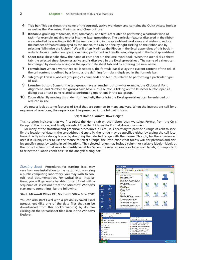
4 Title bar: This bar shows the name of the currently active workbook and contains the Quick Access Toolbaras well as the Maximize, Minimize, and Close buttons.

5 Ribbon: A grouping of toolbars, tabs, commands, and features related to performing a particular kind oftask—for example, making entries into the Excel spreadsheet. The particular features displayed in the ribbonare controlled by selecting a Tab. If the user is working in the spreadsheet workspace and wishes to reducethe number of features displayed by the ribbon, this can be done by right-clicking on the ribbon and byselecting “Minimize the Ribbon.” We will often Minimize the Ribbon in the Excel appendices of this book inorder to focus attention on operations being performed and results being displayed in the Excel spreadsheet.

6 Sheet tabs: These tabs show the name of each sheet in the Excel workbook. When the user clicks a sheettab, the selected sheet becomes active and is displayed in the Excel spreadsheet. The name of a sheet canbe changed by double-clicking on the appropriate sheet tab and by entering the new name.

7 Formula bar: When a worksheet cell is selected, the formula bar displays the current content of the cell. Ifthe cell content is defined by a formula, the defining formula is displayed in the formula bar.

8 Tab group: This is a labeled grouping of commands and features related to performing a particular type of task.

9 Launcher button: Some of the tab groups have a launcher button—for example, the Clipboard, Font,Alignment, and Number tab groups each have such a button. Clicking on the launcher button opens adialog box or task pane related to performing operations in the tab group.

10 Zoom slider: By moving this slider right and left, the cells in the Excel spreadsheet can be enlarged orreduced in size.

We now a look at some features of Excel that are common to many analyses. When the instructions call for asequence of selections, the sequence will be presented in the following form:

Select Home : Format : Row Height

This notation indicates that we first select the Home tab on the ribbon, then we select Format from the CellsGroup on the ribbon, and finally we select Row Height from the Format drop-down menu.

For many of the statistical and graphical procedures in Excel, it is necessary to provide a range of cells to spec-ify the location of data in the spreadsheet. Generally, the range may be specified either by typing the cell loca-tions directly into a dialog box or by dragging the selected range with the mouse. Though, for the experienceduser, it is usually easier to use the mouse to select a range, the instructions that follow will, for precision and clar-ity, specify ranges by typing in cell locations. The selected range may include column or variable labels—labels atthe tops of columns that serve to identify variables. When the selected range includes such labels, it is importantto select the “Labels check box” in the analysis dialog box.

Starting Excel Procedures for starting Excel mayvary from one installation to the next. If you are usinga public computing laboratory, you may wish to con-sult local documentation. For typical Excel installa-tions, you will generally be able to start Excel with asequence of selections from the Microsoft Windowsstart menu something like the following:

Start : Microsoft Office XP : Microsoft Office Excel 2007

You can also start Excel with a previously saved Excelspreadsheet (like one of the data files that can bedownloaded from this book’s website) by double-clicking on the spreadsheet file’s icon in the WindowsExplorer.

bow02371_app1.1.qxd 3/2/11 3:30 PM Page 2

1st Pass

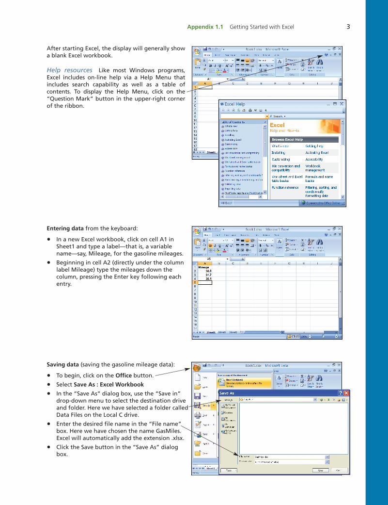
Saving data (saving the gasoline mileage data):

• To begin, click on the Office button.

• Select Save As : Excel Workbook

• In the “Save As” dialog box, use the “Save in” drop-down menu to select the destination driveand folder. Here we have selected a folder calledData Files on the Local C drive.

• Enter the desired file name in the “File name” box. Here we have chosen the name GasMiles. Excel will automatically add the extension .xlsx.

• Click the Save button in the “Save As” dialogbox.

Appendix 1.1 Getting Started with Excel 3

After starting Excel, the display will generally showa blank Excel workbook.

Help resources Like most Windows programs, Excel includes on-line help via a Help Menu that includes search capability as well as a table ofcontents. To display the Help Menu, click on the“Question Mark” button in the upper-right cornerof the ribbon.

Entering data from the keyboard:

• In a new Excel workbook, click on cell A1 inSheet1 and type a label—that is, a variablename—say, Mileage, for the gasoline mileages.

• Beginning in cell A2 (directly under the columnlabel Mileage) type the mileages down thecolumn, pressing the Enter key following eachentry.

bow02371_app1.1.qxd 3/22/11 3:13 PM Page 3

4 Chapter 1 An Introduction to Business Statistics

Retrieving an Excel spreadsheet containing thegasoline mileages:

• Select Office : OpenThat is, click on the Office button and then select Open.

• In the Open dialog box, use the “Look in”drop-down menu to select the source drive andfolder. Here we have selected a folder calledData Files on the Local C drive.

• Enter the desired file name in the “File name”box. Here we have chosen the Excel spread-sheet GasMiles.xlsx.

• Click the Open button in the Open dialog box.

Creating a runs (time series) plot:

• Enter the gasoline mileage data into column A ofthe worksheet with label Mileage in cell A1.

• Click on any cell in the column of mileages, or select the range of the data to be charted bydragging with the mouse. Selecting the range ofthe data is good practice because—if this is notdone—Excel will sometimes try to construct achart using all of the data in your worksheet. Theresult of such a chart is often nonsensical. Here,of course, we only have one column of data—sothere would be no problem. But, in general, it isa good idea to select the data before construct-ing a graph.

• Select Insert : Line : 2-D Line : Line with MarkersHere select the Insert tab and then select Linefrom the Charts group. When Line is selected, agallery of line charts will be displayed. From thegallery, select the desired chart—in this case a 2-D Line chart with markers. The proper chart canbe selected by looking at the sample pictures. Asan alternative, if the cursor is held over a picture,a descriptive “tool tip” of the chart type will bedisplayed. In this case, the “Line with Markers”tool tip was obtained by holding the cursor overthe highlighted picture.

• When you click on the “2-D Line with Markers”icon, the chart will appear in a graphics windowand the Chart Tools ribbon will be displayed.

• To prepare the chart for editing, it is best tomove the chart to a new worksheet called a“chart sheet”. To do this, click on the Design taband select Move Chart.

• In the Move Chart dialog box, select the “Newsheet” option, enter a name for the new sheet—here, “Runs Plot”—into the “New sheet” window,and click OK.

bow02371_app1.1.qxd 3/2/11 3:30 PM Page 4

1st Pass

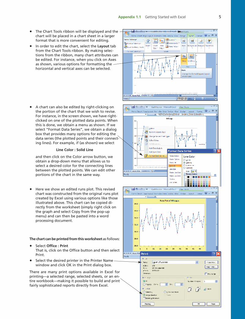
• Here we show an edited runs plot. This revisedchart was constructed from the original runs plotcreated by Excel using various options like those illustrated above. This chart can be copied di-rectly from the worksheet (simply right click onthe graph and select Copy from the pop-upmenu) and can then be pasted into a wordprocessing document.

The chart can be printed from this worksheet as follows:

• Select Office : PrintThat is, click on the Office button and then selectPrint.

• Select the desired printer in the Printer Name window and click OK in the Print dialog box.

There are many print options available in Excel forprinting—a selected range, selected sheets, or an en-tire workbook—making it possible to build and printfairly sophisticated reports directly from Excel.

Appendix 1.1 Getting Started with Excel 5

• The Chart Tools ribbon will be displayed and thechart will be placed in a chart sheet in a larger format that is more convenient for editing.

• In order to edit the chart, select the Layout tabfrom the Chart Tools ribbon. By making selec-tions from the ribbon, many chart attributes canbe edited. For instance, when you click on Axesas shown, various options for formatting the horizontal and vertical axes can be selected.

• A chart can also be edited by right-clicking onthe portion of the chart that we wish to revise.For instance, in the screen shown, we have right-clicked on one of the plotted data points. Whenthis is done, we obtain a menu as shown. If weselect “Format Data Series”, we obtain a dialogbox that provides many options for editing thedata series (the plotted points and their connect-ing lines). For example, if (as shown) we select

Line Color : Solid Line

and then click on the Color arrow button, we obtain a drop-down menu that allows us to select a desired color for the connecting lines between the plotted points. We can edit other portions of the chart in the same way.

bow02371_app1.1.qxd 3/2/11 3:30 PM Page 5

1st Pass

6 Chapter 1 An Introduction to Business Statistics

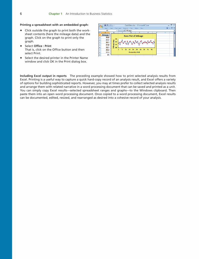
Printing a spreadsheet with an embedded graph:

• Click outside the graph to print both the work-sheet contents (here the mileage data) and thegraph. Click on the graph to print only thegraph.

• Select Office : Print That is, click on the Office button and then select Print.

• Select the desired printer in the Printer Namewindow and click OK in the Print dialog box.

Including Excel output in reports The preceding example showed how to print selected analysis results fromExcel. Printing is a useful way to capture a quick hard-copy record of an analysis result, and Excel offers a varietyof options for building sophisticated reports. However, you may at times prefer to collect selected analysis resultsand arrange them with related narrative in a word processing document that can be saved and printed as a unit.You can simply copy Excel results—selected spreadsheet ranges and graphs—to the Windows clipboard. Thenpaste them into an open word processing document. Once copied to a word processing document, Excel resultscan be documented, edited, resized, and rearranged as desired into a cohesive record of your analysis.

bow02371_app1.1.qxd 3/2/11 3:30 PM Page 6

1st Pass