Clim. Past, 13, 959–975, 2017https://doi.org/10.5194/cp-13-959-2017© Author(s) 2017. This work is distributed underthe Creative Commons Attribution 3.0 License.

Antarctic climate and ice-sheet configuration during the earlyPliocene interglacial at 4.23 MaNicholas R. Golledge1,2, Zoë A. Thomas3, Richard H. Levy2, Edward G. W. Gasson4, Timothy R. Naish1,Robert M. McKay1, Douglas E. Kowalewski5, and Christopher J. Fogwill31Antarctic Research Centre, Victoria University of Wellington, Wellington 6140, New Zealand2GNS Science, Avalon, Lower Hutt 5011, New Zealand3Climate Change Research Centre and PANGEA Research Centre, University of New South Wales,Sydney, NSW 2052, Australia4Department of Geography, The University of Sheffield, Sheffield, S10 2TN, UK5Department of Earth, Environment, and Physics, Worcester State University, Worcester, MA 01602, USA

Correspondence to: Nicholas R. Golledge (nicholas.golledge@vuw.ac.nz)

Received: 22 November 2016 – Discussion started: 5 December 2016Revised: 11 April 2017 – Accepted: 6 June 2017 – Published: 27 July 2017

Abstract. The geometry of Antarctic ice sheets during warmperiods of the geological past is difficult to determine fromgeological evidence, but is important to know because suchreconstructions enable a more complete understanding ofhow the ice-sheet system responds to changes in climate.Here we investigate how Antarctica evolved under orbitaland greenhouse gas conditions representative of an inter-glacial in the early Pliocene at 4.23 Ma, when SouthernHemisphere insolation reached a maximum. Using offline-coupled climate and ice-sheet models, together with a newsynthesis of high-latitude palaeoenvironmental proxy data todefine a likely climate envelope, we simulate a range of ice-sheet geometries and calculate their likely contribution tosea level. In addition, we use these simulations to investi-gate the processes by which the West and East Antarctic icesheets respond to environmental forcings and the timescalesover which these behaviours manifest. We conclude that theAntarctic ice sheet contributed 8.6± 2.8 m to global sea levelat this time, under an atmospheric CO2 concentration iden-tical to present (400 ppm). Warmer-than-present ocean tem-peratures led to the collapse of West Antarctica over cen-turies, whereas higher air temperatures initiated surface melt-ing in parts of East Antarctica that over one to two millennialed to lowering of the ice-sheet surface, flotation of groundedmargins in some areas, and retreat of the ice sheet into theWilkes Subglacial Basin. The results show that regional vari-ations in climate, ice-sheet geometry, and topography pro-

duce long-term sea-level contributions that are non-linearwith respect to the applied forcings, and which under cer-tain conditions exhibit threshold behaviour associated withbehavioural tipping points.

1 Introduction

The response of the Antarctic ice sheets (AIS) to predictedfuture oceanic and atmospheric warming will dictate themagnitude of global sea level changes for millennia, yet thesensitivity of the AIS system is unclear, leading to a widerange of sea-level predictions for coming centuries (Ritzet al., 2015; Golledge et al., 2015; DeConto and Pollard,2016). Simulations of future scenarios such as these are mostcredible when constrained by observations of past changes.Here we simulate the AIS during a warmer period of thegeological past for which geological and paleoenvironmen-tal data exist (Cook et al., 2013; Miller et al., 2012; McKayet al., 2012) with which to verify simulations. Warm periodsof the Pliocene (2.58–5.33 Ma) are considered some of themost appropriate analogues for future environmental condi-tions (Haywood et al., 2016), especially the early to mid-Pliocene (4–5 Ma), when atmospheric CO2 concentrationswere in the range 365–415 ppm (Pagani et al., 2010), sim-ilar to present day. Globally averaged surface temperaturesduring Pliocene interglacials were 2 to > 3 ◦C warmer than

Published by Copernicus Publications on behalf of the European Geosciences Union.

960 N. R. Golledge et al.: Early Pliocene Antarctic ice sheet

present (Haywood et al., 2013), comparable to warmings an-ticipated by 2100 under mid-range emissions scenarios of theIntergovernmental Panel on Climate Change Fifth Assess-ment Report (Collins et al., 2013). Far-field sea-level recordsimply a collapse of the West Antarctic Ice Sheet (WAIS) to-gether with partial loss of marine-based ice from the EastAntarctic Ice Sheet (EAIS) at this time (Miller et al., 2012;Rovere et al., 2014). Geological records from close to theEast Antarctic coast suggest that a portion of this sea-levelcontribution may have originated from the Wilkes SubglacialBasin (WSB), when the ice sheet margin is thought to havemigrated hundreds of kilometres inland (Cook et al., 2013;Patterson et al., 2014).

Given the large scale of these inferred ice-sheet recon-figurations during warm periods of the Pliocene, it may beinferred that Antarctica’s marine-based ice sheets may bevulnerable to thresholds beyond which an abrupt change instate occurs (see Levy et al., 2016; Aitken et al., 2016).If such thresholds exist, and were crossed during Plioceneglacial–interglacial transitions, simulations of ice-sheet evo-lution during this period may be able to provide insights intoprocesses that could be relevant under future warmer cli-mate scenarios. To investigate the sensitivity of Antarctica toclimate–ice-sheet thresholds under warmer climates, we firstrun global and regional climate models to simulate changesin Antarctic oceanic and atmospheric temperatures under anorbital configuration representative of an interglacial in theearly Pliocene at 4.23 Ma, when austral insolation reached amaximum, and atmospheric CO2 concentration was around400 ppm (Figs. 1 and 2). We focus on this period, rather thanthe commonly investigated “PRISM” interval of the mid-Pliocene (Haywood et al., 2013), as the higher insolationand atmospheric CO2 concentration at this earlier time mayhave resulted in a warmer climate and a smaller ice sheetthan the later period, which may help reconcile far-field sea-level records for the period. Outputs from these climate sim-ulations are then used as inputs to ice-sheet model experi-ments that use the Parallel Ice Sheet Model, a fully coupledice-sheet–ice-shelf model (Bueler and Brown, 2009; Winkel-mann et al., 2011). These simulations allow us to quantifythe continental-scale changes that take place under the pre-scribed climatology, and the consequent contribution to sealevel from the AIS. Although the peak climatic conditions wesimulate with the regional-scale climate model (RCM) mostlikely only persisted for 1–2 kyr, we run our simulations for10 kyr in order to quantify how the perturbed ice sheet mightevolve if such warm conditions were maintained. Althoughthis does not realistically reflect climatic forcings associatedwith orbital cyclicities, and implies that our sea-level esti-mates may be upper bounds for the prescribed climates, itis nonetheless a useful approach for the study of “unforced”ice-sheet oscillations, or “tipping points” (Thomas, 2016). Inthe final part of our study, therefore, we use our long-termice-sheet simulations to investigate whether evidence for tip-

450

500

550

600

Inso

latio

n (

W m

−2)

450

500

550

600

Inso

latio

n (

W m

−2)

450

500

550

600

Inso

latio

n (

W m

−2)

−4250 −4245 −4240 −4235 −4230 −4225 −4220

Time (Kyr BP)

450

500

550

600

Inso

latio

n (

W m

−2)

−4250 −4245 −4240 −4235 −4230 −4225 −4220

Time (Kyr BP)

−0.05

0.00

0.05

Pre

ce

ssio

n

−0.05

0.00

0.05

Pre

ce

ssio

n

0.38

0.40

0.42

Ob

liqu

ity

0.38

0.40

0.42

Ob

liqu

ity

0.00

0.02

0.04

0.06

Ecce

ntr

icity

−5000 −4750 −4500 −4250 −4000 −3750 −3500

Time (Kyr BP)

0.00

0.02

0.04

0.06

Ecce

ntr

icity

−5000 −4750 −4500 −4250 −4000 −3750 −3500

Time (Kyr BP)

Figure 1. Orbital components and net January insolation at 80◦ Sfor the period 3.5–5 Ma. Top panel shows insolation for the inter-glacial in which peak Pliocene values occur (grey shading). Theinsolation peak occurs at 4.23 Ma. Data from Laskar et al. (2004).

ping points can be seen, and if so, the mechanisms that giverise to them.

2 Methods

2.1 Climate and ocean inputs

We use spatially distributed air temperature, precipitation,and sea-surface temperatures from an established RCM cou-pled with the GENESIS version 3.0 global climate model(GCM) (Thompson and Pollard, 1997; Pal et al., 2007). TheGCM parameterizes fluxes between the land surface bound-ary and the free atmosphere and includes detailed repre-sentations of snow and land ice. Outputs from the GENE-SIS model have been validated against observed polar cli-mates and ice-sheet mass balance (Thompson and Pollard,1997), and are therefore considered reliable for studies suchas ours. Our RCM is RegCM3, which takes time-dependentlateral boundary conditions from the GCM. It simulates at-mospheric dynamics, radiative transfer, and precipitation,and includes a representation of the open ocean (Pal et al.,2007). RCM simulations at 40 km resolution are initializedfrom coarser-resolution (T31) GCM outputs. We simulatethe climate during a peak-insolation interglacial at 4.23 Mabased on an orbital configuration representative of that pe-

Clim. Past, 13, 959–975, 2017 www.clim-past.net/13/959/2017/

N. R. Golledge et al.: Early Pliocene Antarctic ice sheet 961

210 220 230 240 250 260 270 280

Air temperature (K)

0.0 0.2 0.4 0.6 0.8 1.0

Precipitation (ma−1)

271.0 271.5 272.0 272.5 273.0

Sea surface temperature (K)

PD−CTRL PD−CTRL PD−CTRL

PD−RCM PD−RCM PD−RCM

PLIO−RCM PLIO−RCM PLIO−RCM

Figure 2. Air temperature, precipitation, and sea surface temperature used for our simulations. Top row: the “control” (CTRL) scenario,employing gridded data from observations and modelling of present-day conditions (Comiso, 2000; Lenaerts et al., 2012; Thompson andPollard, 1997; Pal et al., 2007). Middle row: present-day conditions as simulated by the RCM. Bottom row: Pliocene conditions at 4.23 Maas simulated by the RCM.

riod (Fig. 1), together with a greenhouse gas concentration of400 ppm. Although previous work has suggested that the rel-ative role of insolation and CO2 in driving warmer climatesvaries through time, and that high insolation in one hemi-sphere may not necessarily lead to elevated temperatures atthe same latitudes (Yin and Berger, 2012), palaeoenviron-mental proxies for this period are consistent with this beingan interval of peak warmth (see “Palaeoenvironmental prox-ies” below) and fundamentally the ice-sheet responds only tothe integrated warming anomaly, not insolation or radiativeforcing in isolation.

Temperature and precipitation fields from the PlioceneRCM simulation are used as inputs to the ice-sheet modelby calculating the anomalies from a present-day RCM sim-ulation and then adding these to the present-day tempera-ture and precipitation fields used in model initialization andspinup (Figs. 2–4). This approach is preferable to one thatuses the RCM fields directly, since the RCM does not sim-

ulate the present-day state precisely, when compared to ob-servational data (Fig. 2). Since the climate model also usesan ice-sheet topography in which WAIS is already removed,we use a standard lapse rate of 8 K km−1 to adjust the simu-lated temperatures based on the elevation difference from ourpresent-day ice geometry. Despite this adjustment, however,it is possible that the air temperatures in these areas may beanomalously warm as a result of ocean–atmosphere heat ex-change that would not occur if the removed ice were presentin the RCM simulation. This may have an influence of theretreat rate of West Antarctica in our simulations, but sinceour focus lies mainly on the behaviour of the East Antarcticice sheet we do not expect this issue to affect our findings.We do not apply any lapse rate adjustment to precipitationvalues on the basis that precipitation rates are likely to becontrolled largely by synoptic patterns (which are capturedby the RCM) rather than by a simple elevation-dependentcooling of the near-surface atmosphere. Since the RCM uses

www.clim-past.net/13/959/2017/ Clim. Past, 13, 959–975, 2017

962 N. R. Golledge et al.: Early Pliocene Antarctic ice sheet

an ice-sheet geometry in which WAIS is absent it gives us asea-surface temperature field for areas of our domain wheregrounded ice currently persists. However, these ocean tem-peratures are only used to calculate basal melt beneath iceshelves, not at the bed of grounded ice, and so do not affectthe ice sheet unless the modelled grounding line retreats. Forareas of grounded ice where we do not have RCM-derivedocean temperatures we prescribe a uniform value of 271.2 K,essentially the sea-water freezing point. This avoids potentialerrors that could be introduced by interpolating ocean fieldslandward, but we recognize that using a single, low, valuerather than an interpolation may lead to underestimated basalmelt in subglacial basins during ice-sheet retreat. Our offline,one-way climate–ice-sheet model coupling is less satisfac-tory than a two-way coupling, but is computationally easierand allows first-order ice-sheet responses to climate pertur-bations to be investigated. However, we acknowledge that afully coupled setup might give more accurate ice-sheet andclimate simulations.

2.2 Palaeoenvironmental proxies

Local records of palaeo-temperature around the Antarcticcontinent are relatively sparse, yet those that exist, and canbe chronologically constrained with some certainty, offer ameans by which climate model simulations can be evaluated.We compiled marine paleoenvironmental data from severalcircum-Antarctic locations that include drill cores from thewestern Ross Sea (CIROS-2, DVDP-10, AND-2A), PrydzBay (ODP 1165), Kerguelen Plateau (ODP 751A), WilkesLand (IODP U1361), and northwestern Antarctic Peninsula(ODP 1096) and geological outcrop at the Prydz Bay coast(Fig. 3). Data were obtained from stratigraphic intervals thatspan 4.5 to 4.0 Ma (C3n.1r to lowermost C2Ar) which ischaracterized by relatively depleted values (< 3.2 ‰) in thebenthic δ18O stack (Lisiecki and Raymo, 2005) (i.e. rela-tively warm glacials and interglacials; MIS CN1 and CN5 aretwo of the warmest interglacials in the early Pliocene). Seawater temperature estimates through this interval are basedon a range of proxies including biological analogues and geo-chemical data that are described in detail below and whichare summarized in Table 1.

Surface water temperatures from biological proxies are de-rived from diatom, silicoflagellate, and calcareous nannofos-sil data. Diatom assemblages within the target “warm” inter-val at all of the drill sites contain, and are often dominatedby, open ocean species Thalassionema nitzschioides and Sh-ionodiscus tetraoestrupii (Whitehead and Bohaty, 2003a;Winter et al., 2010). Modern descendants of T. nitzschiodesand S. tetraoestrupii are restricted to areas north of the PolarFront where surface water temperatures are greater than 3.5and 5.5 ◦C respectively (Winter et al., 2010; Crosta et al.,2005). Numbers of Azpeitia spp. also increase within theearly Pliocene section at IODP Site U1361 (Cook et al.,2013) and reach a maximum abundance of 13 %. Today

Azpeitia tabularis is considered cold-tolerant in SouthernOcean waters but species abundance increases as water tem-peratures increase and generally exceeds 10 % near the mod-ern subtropical front (Romero et al., 2005), which suggeststhat early Pliocene summer sea surface temperatures at SiteU1361 were as high as 10 ◦C. Importantly, sea-ice-associateddiatom taxa are either rare to absent at most of the drill sites(Winter et al., 2010) or indicate much reduced sea ice cov-erage (Whitehead et al., 2005). Overall, the diatom assem-blages indicate that surface water temperatures at locationssouth of 60◦ in the early Pliocene were similar to those inmodern sub-Antarctic regions and that the circum-Antarcticocean was sea-ice-free throughout most or all of the annualcycle.

Relatively warm early Pliocene surface water tempera-tures implied by the diatom assemblages are supported bysilicoflagellate data. In the modern marine environment thesilicoflagellate genus Distephanus is dominant south of theAntarctic polar front and the genus Dictyocha is rare or ab-sent. The ratio of these genera in ancient sediment samplescan be used to infer past ocean temperature. Dictyocha abun-dance at Ocean Drilling Program Site 1165 increases be-tween 4.3 and 4.4 Ma, which suggests that mean annual SSTincreased to approximately 4 ◦C during this interval (White-head and Bohaty, 2003b). A correlative interval in ODP Sites748 and 751 contains a similar warming signal (Bohaty andHarwood, 1998).

Although temperature reconstructions based on geochem-ical proxies are rare, TEXL86-derived SST estimates of5± 4 ◦C were obtained from diatomite that was depositedbetween 4.5 and 4.2 Ma at the AND-1B drill site (McKayet al., 2012). These data support the temperature reconstruc-tions based on biological proxies and indicate that summersurface water temperatures in the western Ross Sea were 5to 6 ◦C warmer than today. Furthermore, sedimentary faciesindicate increased sediment input during interglacials (Motif2b of McKay et al., 2009; Naish et al., 2009). This is inter-preted as representing a warmer glacial regime (compared tothe late Pliocene) with more sediment-laden meltwater ema-nating from the margins of the EAIS and discharging into theRoss Sea.

Other evidence for warmth in the early Pliocene comesfrom fossil invertebrates and a unique assemblage of verte-brates preserved in the Sørsdal Formation, which crops outat Marine Plain in the Vestfold Hills (Fig. 3). The formationcomprises up to 7.2 m of friable diatomaceous siltstone andsandstone with dark limestone lenses (Quilty et al., 2000).The age of the deposit is not well constrained, but diatomdata suggest it was deposited between 4.4 and 2.74 Ma, andmost likely at the earlier end of this range, possible 4.2 to4.1 Ma (Clark et al., 2013). Cetacean fossils include a speciesof dolphin, a beaked whale, and baleen whale (Quilty et al.,2000; Fordyce et al., 2002). These noncryophilic speciesindicate that waters were ice-free during summer (Fordyceet al., 2002). The Sørsdal Formation also contains the scal-

Clim. Past, 13, 959–975, 2017 www.clim-past.net/13/959/2017/

N. R. Golledge et al.: Early Pliocene Antarctic ice sheet 963

Table 1. Inferred high southern latitude winter, summer, and mean annual sea-surface temperatures from a range of proxy techniquescompared to model predictions. Winter temperatures assume sea ice close to the coast but not in open water. Summer temperatures (and thusTmean also) are minima, and could be higher. Absolute sea-surface temperature predictions from the RCM shown for each site in italics.Although the considerable uncertainties associated with temperature inferences from palaeoecological proxies make precise comparisonsimpossible, the data generally indicate an underestimate of mean annual sea-surface temperatures in the RCM that averages approximately1 ◦C.

Site Long Lat Winter Summer Tmean Reference(likely) (min.) (min.)

AND-1B 167.083333 −77.888889 −1.8 5 1.6 Winter et al. (2010), McKay et al. (2012)–2.22 3.03 –0.22

CIROS-2 163.533333 −77.683333 −1.8 5 1.6 Winter (1995), Levy et al. (2012)–1.96 3.29 0.07

DVDP-10 163.511667 −77.578612 −1.8 5 1.6 Winter (1995), Levy et al. (2012)–1.96 3.29 0.08

ODP-1165 67.218733 −64.379583 3 5 4 Whitehead and Bohaty (2003b), Cook et al. (2014)–0.02 7.19 3.54

IODP-U1361 143.886653 −64.409547 3 5 4 Cook et al. (2013)–0.43 6.24 2.87

ODP-1096 −76.96376 −67.56681 −1.8 5 1.6 Winter and Iwai (2002)–1.87 4.80 1.26

Vestfold Hills 78.132 −68.631111 −1.8 5 1.6 Whitehead et al. (2001)–0.99 6.00 2.37

0

5

5

5

55

10

10 10

Wilkes

0 5 10 15 20 25

Plio dT (K)

0.5

0.5

1

1

1

1

1

1

1

1.5

1.5

1.5

1.5

1.5

1.5

1.5

2

2

2

2

2

2

2

2

2

2

2.5

2.5

2.5

2.5

2.5

2.5

2.5

2.5

2.5

2.5

3

3

3

3

3

3

3

3

3

3

3

3

3.5

3.5

3.5

3.5

3.5

3.5

3.5

3.5

3.5

3.53.5

3.5

3.5

4

4

4 4

4

4 4

4

4

4

4

4.5

4.5

4.5

AND−1B

CIROS−2

DVDP−10

ODP−1165

IODP−U1361

ODP−1096 Vestfold Hills

0 1 2 3 4 5

Plio dSST (K)

( a) ( b)

Figure 3. (a) Air temperature anomaly for 4.23 Ma from regional climate modelling, adjusted for surface elevation differences betweenthe RCM input orography and the present-day elevations used to initialize the ice-sheet model. Contours show 2.5 ◦C increments. Biasesused in certain simulations are additional to the warming values shown here. (b) As (a) but showing sea-surface temperature anomaly.Contours show 0.25 ◦C increments. Locations of profile shown in Fig. 7 also shown (red line), as well as the locations (red squares) of thepalaeo-environmental proxy data in Table 1.

lop Austrochlamys anderssoni. This and similar species ofthick-shelled costate scallop thrived in Antarctic waters dur-ing interglacial episodes throughout the Neogene but disap-peared during the late Pliocene (Jonkers, 1998). Modern de-scendants of these thick-walled species do not live furthersouth than sub-Antarctic regions where surface water tem-

peratures are warmer than 5.5 ◦C. Diatoms in the formationalso indicate an annual range in SST from −1.8 to 5.0 ◦C(Whitehead et al., 2001) and the absence of coccoliths in-dicates that summer SSTs were likely no higher than 5 ◦C(Whitehead et al., 2001).

www.clim-past.net/13/959/2017/ Clim. Past, 13, 959–975, 2017

964 N. R. Golledge et al.: Early Pliocene Antarctic ice sheet

In summary, the evidence listed above indicates that sum-mertime surface water temperatures in the early Pliocenewere at least as high as 4–5 ◦C during the warmest inter-glacial periods, and were likely warmer at 64◦ S (IODP siteU1361). Evidence for minimal sea ice suggests that whilewinter water temperatures may have approached −1.8 ◦C,summers were sea-ice-free. Based on these data we infer thatearly Pliocene surface water temperatures in the oceans ad-jacent to Antarctica’s continental ice sheets must have beenhigher than −1.8 ◦C in the winter and at least 5 ◦C in thesummer – a mean annual temperature that was approximately3 ◦C warmer than today. Table 1 compares these proxy-basedinterpretations with values simulated by our climate modelexperiments.

2.3 The ice-sheet model

Our ice-sheet simulations use the Parallel Ice Sheet Model(PISM) version 0.6.3, an open-source, three-dimensional,thermodynamic, coupled ice-sheet–ice-shelf model. Both themodel and our implementation of it are described in detailelsewhere (Bueler and Brown, 2009; Golledge et al., 2015;Aitken et al., 2016), so only a summary is given here. Inbrief, the model combines equations of the shallow-ice andshallow-shelf approximations (SIA and SSA respectively)for grounded ice, and uses the SSA for floating ice (Buelerand Brown, 2009). Superposing the SIA and SSA velocitysolutions allows basal sliding to be simulated according tothe “dragging shelf” approach (Bueler and Brown, 2009),and enables a consistent treatment of stress regime across thegrounded to floating ice transition (Winkelmann et al., 2011).Ice streams develop naturally as a consequence of plastic fail-ure of saturated basal till (Schoof, 2006), depending on thethermal regime and volume of water at the ice-sheet bed. Be-cause we employ a large number of simulations in our study,we adopt a relatively coarse model grid of 20 km. Mesh de-pendence of results can be an important issue under certaincircumstances (Martin et al., 2015), but in previous workwe have shown that this is not the case in our simulations(Golledge et al., 2015). Furthermore, the principal aim ofour experiments is to identify differences between scenarios,rather than to define absolute ice geometries, and for this pur-pose we believe our approach is both suitable and robust.

Grounding-line migration is a key component of Antarc-tic ice-sheet simulations, and is a much-debated modellingchallenge. By default we adopt here a novel grounding-line scheme that uses a sub-grid interpolation method tomore accurately track migrations (Feldmann et al., 2014).In this scheme we allow the sub-grid interpolation of driv-ing stress at the bed, and the calculation of one-sided deriva-tives to better characterize the ice-sheet–shelf junction. Werun duplicate experiments both with and without an addi-tional interpolation scheme that allows basal melt rates tobe smoothly propagated across the grounding line from thefirst floating cell upglacier to the last grounded cell (Feld-

Table 2. Mass loss in sea-level equivalent metres from the simu-lated Pliocene Antarctic ice sheet after 10 kyr, using environmentalconditions from the regional climate model and augmented with arange of air and ocean temperature bias corrections. Numbers inparentheses represent duplicate experiments in which a more ag-gressive grounding-line scheme is employed (see “Methods”).

Sea-surface temperature bias

0 1 2

Air 0 4 (4.6) 6 (8.7) 7.9 (12.2)temp. 1 5.6 (6.2) 7.7 (9.4) 8.8 (13)bias 2 7.7 (8.4) 9.1 (10.9) 10.3 (14.1)

mann et al., 2014; Feldmann and Levermann, 2015). Thismechanism tends to accelerate grounding-line retreat, lead-ing to rapid mass loss in the initial centuries of the exper-iments, and greater long-term (near-equilibrium) sea-level-equivalent mass loss from the simulated ice sheets (Ta-ble 2). It is conceptually supported by geophysical studiesof modern-day grounding lines that infer an “estuarine”-typeenvironment at ice-stream grounding zones (Horgan et al.,2013), and although less catastrophic than the cliff-collapsemechanism used in other models (Pollard et al., 2015; De-Conto and Pollard, 2016) the approach is consistent withrecent grounding-line process analyses (Gladstone et al.,2016). Basal melt beneath ice shelves (and at the ground-ing line) is calculated from a three-equation model that usestemperature, salinity, and pressure to determine the freezingpoint in the boundary layer (Hellmer et al., 1998; Hollandand Jenkins, 1999). Depending on whether there is melt,freeze-on, or neither, a different approximation of the tem-perature at the ice-shelf base is used. Outputs from RegCM3do not include subsurface ocean temperatures, and further-more, PISM is currently set up to read in just a single oceantemperature field. Consequently we are not able to investi-gate how vertical differences in ocean warming may impactthe ice sheet. Our model does, however, allow the pressureeffects of deeper bathymetry to be accounted for, giving riseto enhanced basal melt near grounding lines and less meltin central and outer sectors of the shelf (see Golledge et al.,2017, Fig. S5).

Surface mass balance depends on monthly climatologi-cal data and a positive degree-day model that tracks snowthickness and allows for melting of snow and ice at 3 and8 mm ◦C−1 day−1 respectively. We incorporate a white noisesignal (normally distributed, mean zero random temperatureincrement) into the calculation of daily temperature varia-tions. The standard deviation of daily temperature variabil-ity is set at 2 ◦C, somewhat lower than the commonly em-ployed value of 5 ◦C, on the basis that the latter has a ten-dency to overestimate melt (Seguinot, 2013; Rogozhina andRau, 2014). Surface temperatures are adjusted for elevationaccording to an altitudinal lapse rate of−8 K km−1, and a re-

Clim. Past, 13, 959–975, 2017 www.clim-past.net/13/959/2017/

N. R. Golledge et al.: Early Pliocene Antarctic ice sheet 965

freezing coefficient of 0.6 is used to mimic meltwater capturewithin the snowpack.

2.4 Experimental methods

There are two approaches to dealing with ice model parame-ter uncertainty in the kind of study we present here. One ap-proach undertakes thousands of low-resolution experiments(a large ensemble) with incremental changes in each of sev-eral key parameters, such as flow enhancement factors. Theresults are then subsequently analysed with respect to ob-servational constraints to establish which ensemble membersare consistent with the data. We do not adopt this kind ofapproach. Instead we follow a more targeted methodologyin which model parameter choice is incrementally refinedthrough an iterative procedure in which we constrain ourmodel to fit the present-day ice-sheet geometry and surfacevelocity field. To achieve a good fit we adjust ice flow param-eters based on expert judgement, not in an unguided manneras is done with ensemble approaches. We start with an ini-tial 20-year smoothing run that uses only the shallow-ice ap-proximation to derive velocities. This removes spurious sur-face irregularities. Secondly, we implement a 150 000-yearrun in which the ice-sheet geometry is held fixed but whereinternal thermal fields are allowed to evolve. The third phaseuses a 25 000-year simulation in which full model physicsare employed and the ice sheet is allowed to evolve on allboundaries – that is, it is entirely unconstrained. Throughcarefully guided parameter iteration our procedure results ina spun-up, thermally and dynamically equilibrated ice-sheetsimulation that is the best fit to observational constraints thatis possible by tuning available model parameters (Golledgeet al., 2015; Aitken et al., 2016). Thus although parameteruncertainty can be a large source of error under certain cir-cumstances (see Yan et al., 2016), we argue that our approachsignificantly reduces this uncertainty prior to our undertakingthe prognostic experimentation. All experiments start fromthe same spun-up present-day ice-sheet simulation.

We make an assumption regarding the state of the AISprior to the interglacial at 4.23 Ma based on geological ev-idence that indicates ice extent greater than present duringearly Pliocene glacial episodes (Naish et al., 2009), imply-ing that the AIS retreated through a present-day configura-tion during interglacial transitions. However, since the ini-tial condition of the ice sheet is not known, our assumptionof a present-day configuration may be erroneous. However,differences in initial geometry would most likely affect therate at which new equilibria to the imposed climatologiesoccurred, rather than the geometries of those steady states.Consequently we consider our equilibrium simulations tobe representative of the likely long-term Antarctic responseto the prescribed orbital and greenhouse gas configuration.We use outputs from the RCM (described above) to defineanomalies to our present-day climate grids (Comiso, 2000;Lenaerts et al., 2012). Simulations are run for 10 kyr, which

is long enough for most simulations to approach a steadystate (see “Results” below). We first model ice-sheet evolu-tion using climate fields simulated by the RCM, using bothimplementations of the sub-grid grounding-line scheme de-scribed above. Then we explore the threshold response of theEAIS by running additional experiments with uniform incre-ments of 1 and 2 ◦C added to the air and sea-surface tem-perature fields, which address both a known cold bias in theRCM as well as mismatches between RCM and proxy-basedtemperature reconstructions. By bracketing a range of tem-peratures we are also able to investigate more easily the exis-tence and sensitivity of the AIS to climate–ice-sheet thresh-olds. To isolate the effects of the imposed climatic pertur-bations most clearly we keep sea level at its modern level,rather than the +10 to +30 m thought likely for the Pliocene(Miller et al., 2012; Rovere et al., 2014; Winnick and Caves,2015). We note, however, that in separate experiments notshown here the response of the ice sheet appears to be un-affected by sea level changes of these magnitudes. We runduplicates of all experiments using the two variants of thesub-grid grounding-line scheme described above.

2.5 Tipping point analysis

The aim of this technique is to analyse time series data (inour case ice mass evolution) to find early warning signs ofimpending tipping points. Such events are characterized bya non-linear response to an underlying forcing, based on thephenomenon of “critical slowing down”, and relies on thegradual shallowing and widening of the state-space of thesystem (also known as the “basin of attraction”) (Schefferet al., 2009, 2012). This “slowing down” can be mathemati-cally detected by looking at the pattern of fluctuations in theshort-term trends of the data before the threshold is passed(Dakos et al., 2008). This change in shape of the state-spaceallows the system to travel further from its point of equilib-rium (van Nes and Scheffer, 2007), whereupon the systemtakes increasingly longer to recover from small perturbations(Dakos et al., 2012), which can be detected as an increasein the lag-1 autocorrelation and variance of the time series(Ives, 1995). A change in skewness may also be interpretedas a precursor to tipping (Guttal and Jayaprakash, 2008).

This tipping point analysis technique has been applied toa range of climate and palaeoclimate data using both natu-ral archives and model outputs (Dakos et al., 2008; Lentonet al., 2012; Thomas et al., 2015; Thomas, 2016; Turneyet al., 2015). Importantly, the early warning signs, or precur-sors, are only expected in the presence of two or more quasi-stationary states, separated by an unstable equilibrium, andare not expected in the case of tipping induced by stochasticfluctuations only, so their identification tends to imply a realthreshold change. The method (Dakos et al., 2008; Guttal andJayaprakash, 2008; Dakos et al., 2012) only analyses datapreceding the tipping point. These data are detrended using aGaussian kernel smoothing filter over a suitable bandwidth,

www.clim-past.net/13/959/2017/ Clim. Past, 13, 959–975, 2017

966 N. R. Golledge et al.: Early Pliocene Antarctic ice sheet

so that long-term trends are removed without overfitting thedata. The resulting residuals are then measured for autocor-relation at lag-1 and variance over sliding windows of twodifferent sizes. The Kendall tau rank correlation coefficient(Kendall, 1948) is used to provide a quantitative measureof the trend; this metric varies between +1 and −1, wherehigher values indicate a greater concordance of pairs and astronger increasing trend. Importantly, it is the presence of aparallel increasing trend in both autocorrelation and variance,rather than the absolute values of the indicators, that indicatescritical slowing down (Ditlevsen and Johnsen, 2010).

For the purposes of this study we make an important dis-tinction between a tipping point and a threshold, which aresometimes used synonymously. We define a tipping point asa transient feature, whereas a threshold is non-temporal. Dur-ing the evolution of an ice sheet under a constant forcing itmay be that a point is reached in which the trajectory of evo-lution changes, i.e. the system “tips” into a new state of be-haviour. By analysing the time series data from a constantforcing experiment, tipping point analysis is able to not onlyshow where genuine system instabilities occur, but also toprovide information on the timescale over which this insta-bility evolves. This is what the final part of our study investi-gates. However, this point of change, under a steady forcing,is not the same as the identification of a single temperature atwhich the ice sheet may be stable or unstable in a given areaand over a discrete period of time. Consequently it is not pos-sible from our tipping point analysis to provide informationon a threshold, as the two phenomena are simply differententities. A detailed explanation of tipping points in Earth sys-tems can be found in Thomas (2016), whereas threshold tem-peratures for individual Antarctic ice-sheet catchments havebeen quantified in Golledge et al. (2017).

3 Results

For the first of our experiments, we run our RCM to sim-ulate the early Pliocene climate at 4.23 Ma. The modelyields spatially variable annual air and sea-surface temper-ature changes whose means are approximately 5 and 2 ◦Cabove present respectively, for presently ice-covered areas ofAntarctica (Figs. 3 and 4). The advantage of using a knownperiod of the past such as this, rather than a forward pro-jection, is that we can use empirical data to evaluate ourmodelled climate fields and to constrain our ice-sheet sim-ulations. Proxy data suggest that our simulated climate maybe 1–2 ◦C cooler than actually occurred (Table 1); thus, werun duplicate simulations allowing for additional warmingof 1 and 2 ◦C in both the atmosphere and ocean. The sea-level equivalent ice volume loss from Antarctica in thesesimulations ranges from 4 to 14 m (Table 2; Fig. 5). As-suming a 5 to 7 m contribution from the Greenland ice sheet(Koenig et al., 2015) and 0.5 to 1 m from thermal expansionof the oceans (assuming 1 to 3 ◦C ocean warming) (Rugen-

0

1

2

3

4

5

6

Fre

quency (

%)

−2 0 2 4 6 8 10 12 14 16 18 20 22 24

RCM p liocene warming (K)

S ea surface mean = 3 ± 1.1 K (mode = 3.6 K)

S ub−shelf mean = 1.9 ± 0.94 K (mode = 2 K)

L and surface mean = 7.2 ± 4.9 K (mode = 4.9 K)

Figure 4. Histogram representation on the anomaly data shown inFig. 3. Biases used in certain simulations are additional to the warm-ing values shown here. Note the very long tail that skews the meanvalue of modelled land surface warming, indicating that the modalvalue might be most representative of the continent as a whole. Sea-surface temperature anomalies are also higher in the open oceanthan those of a subset representing ocean areas where present-dayice shelves exist.

stein et al., 2016), all of our simulations are consistent witha Pliocene sea level highstand range of approximately 10 to> 20 m reconstructed from proxy records (Miller et al., 2012;Rovere et al., 2014; Winnick and Caves, 2015). However, byconsidering likely air–ocean temperature relationships (Ru-genstein et al., 2016), as well as empirical records of an ab-sent WAIS and a retreated EAIS at this time (Naish et al.,2009; Cook et al., 2013), we are able to identify two sce-narios as most plausible. Figure 6a and b illustrate the mod-elled Antarctic ice-sheet geometry that arises under constantforcing with the Pliocene climate, modified to incorporate a+2 ◦C air temperature bias and a 0 or 1 ◦C bias in the ocean(see “Methods”). In both cases we reproduce the smaller-than-present ice geometry, as well as the pattern of basal icevelocities that would have controlled bedrock erosion andsediment transport, that are necessary to be consistent withgeological interpretations (Naish et al., 2009; Cook et al.,2013).

In both of the scenarios shown in Fig. 6, substantialgrounding-line retreat is evident in the WSB, but the Auroraand Recovery basins are less affected. To better understandthe timescales and rates involved in retreat in the WSB, wetake timeslice ice and bed geometries along the WSB flow-line from the two simulations considered representative ofPliocene conditions at 4.23 Ma (Fig. 6a, b). In both scenar-ios, we find that margin retreat under constant climate forc-ing is punctuated by periods of stability. Figure 7a illustratesa gradual surface lowering at the margin of the ice sheet thatcontinues for 2000 years before flotation and grounding-lineretreat ensue. At this point, rapid retreat takes place across

Clim. Past, 13, 959–975, 2017 www.clim-past.net/13/959/2017/

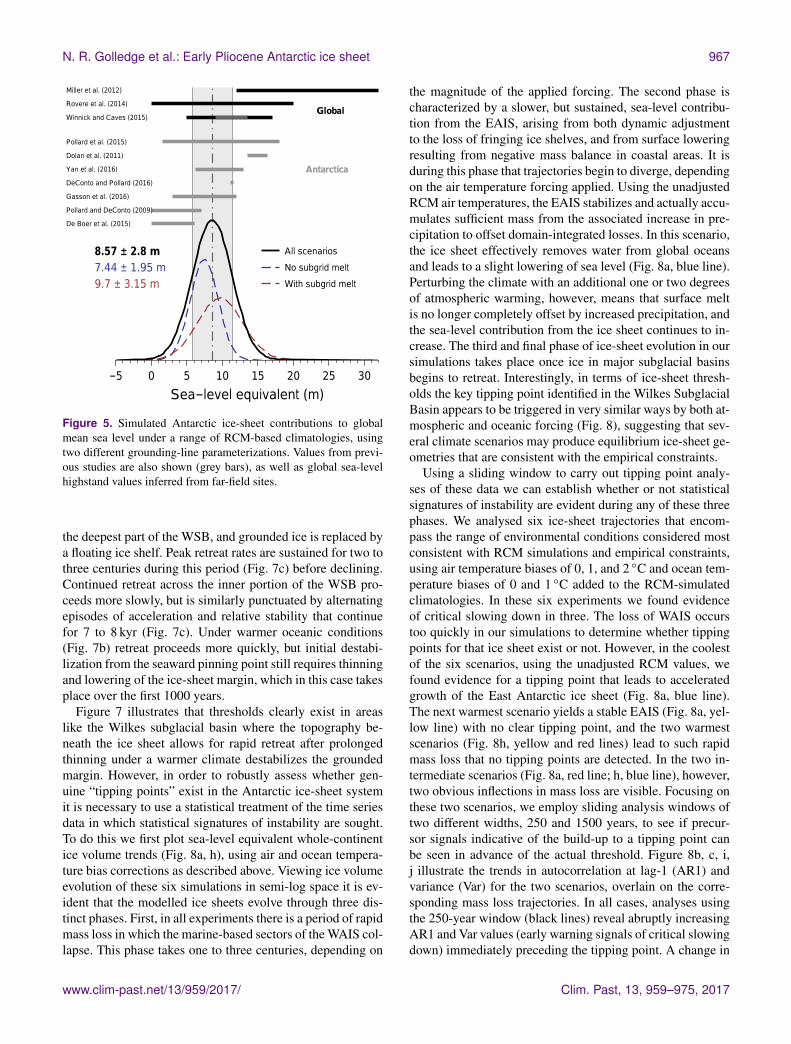
N. R. Golledge et al.: Early Pliocene Antarctic ice sheet 967

−5 0 5 10 15 20 25 30

Sea−level equivalent (m)

8.57 ± 2.8 m

7.44 ± 1.95 m

9.7 ± 3.15 m

A ll scenarios

N o subgrid melt

With subgrid melt

Miller et al. (2012)

Rovere et al. (2014)

Winnick and Caves (2015)

Pollard et al. (2015)

Dolan et al. (2011)

Yan et al. (2016)

DeConto and Pollard (2016)

Gasson et al. (2016)

Pollard and DeConto (2009)

De Boer et al. (2015)

Gl o b a l

An t a r c t i c a

Figure 5. Simulated Antarctic ice-sheet contributions to globalmean sea level under a range of RCM-based climatologies, usingtwo different grounding-line parameterizations. Values from previ-ous studies are also shown (grey bars), as well as global sea-levelhighstand values inferred from far-field sites.

the deepest part of the WSB, and grounded ice is replaced bya floating ice shelf. Peak retreat rates are sustained for two tothree centuries during this period (Fig. 7c) before declining.Continued retreat across the inner portion of the WSB pro-ceeds more slowly, but is similarly punctuated by alternatingepisodes of acceleration and relative stability that continuefor 7 to 8 kyr (Fig. 7c). Under warmer oceanic conditions(Fig. 7b) retreat proceeds more quickly, but initial destabi-lization from the seaward pinning point still requires thinningand lowering of the ice-sheet margin, which in this case takesplace over the first 1000 years.

Figure 7 illustrates that thresholds clearly exist in areaslike the Wilkes subglacial basin where the topography be-neath the ice sheet allows for rapid retreat after prolongedthinning under a warmer climate destabilizes the groundedmargin. However, in order to robustly assess whether gen-uine “tipping points” exist in the Antarctic ice-sheet systemit is necessary to use a statistical treatment of the time seriesdata in which statistical signatures of instability are sought.To do this we first plot sea-level equivalent whole-continentice volume trends (Fig. 8a, h), using air and ocean tempera-ture bias corrections as described above. Viewing ice volumeevolution of these six simulations in semi-log space it is ev-ident that the modelled ice sheets evolve through three dis-tinct phases. First, in all experiments there is a period of rapidmass loss in which the marine-based sectors of the WAIS col-lapse. This phase takes one to three centuries, depending on

the magnitude of the applied forcing. The second phase ischaracterized by a slower, but sustained, sea-level contribu-tion from the EAIS, arising from both dynamic adjustmentto the loss of fringing ice shelves, and from surface loweringresulting from negative mass balance in coastal areas. It isduring this phase that trajectories begin to diverge, dependingon the air temperature forcing applied. Using the unadjustedRCM air temperatures, the EAIS stabilizes and actually accu-mulates sufficient mass from the associated increase in pre-cipitation to offset domain-integrated losses. In this scenario,the ice sheet effectively removes water from global oceansand leads to a slight lowering of sea level (Fig. 8a, blue line).Perturbing the climate with an additional one or two degreesof atmospheric warming, however, means that surface meltis no longer completely offset by increased precipitation, andthe sea-level contribution from the ice sheet continues to in-crease. The third and final phase of ice-sheet evolution in oursimulations takes place once ice in major subglacial basinsbegins to retreat. Interestingly, in terms of ice-sheet thresh-olds the key tipping point identified in the Wilkes SubglacialBasin appears to be triggered in very similar ways by both at-mospheric and oceanic forcing (Fig. 8), suggesting that sev-eral climate scenarios may produce equilibrium ice-sheet ge-ometries that are consistent with the empirical constraints.

Using a sliding window to carry out tipping point analy-ses of these data we can establish whether or not statisticalsignatures of instability are evident during any of these threephases. We analysed six ice-sheet trajectories that encom-pass the range of environmental conditions considered mostconsistent with RCM simulations and empirical constraints,using air temperature biases of 0, 1, and 2 ◦C and ocean tem-perature biases of 0 and 1 ◦C added to the RCM-simulatedclimatologies. In these six experiments we found evidenceof critical slowing down in three. The loss of WAIS occurstoo quickly in our simulations to determine whether tippingpoints for that ice sheet exist or not. However, in the coolestof the six scenarios, using the unadjusted RCM values, wefound evidence for a tipping point that leads to acceleratedgrowth of the East Antarctic ice sheet (Fig. 8a, blue line).The next warmest scenario yields a stable EAIS (Fig. 8a, yel-low line) with no clear tipping point, and the two warmestscenarios (Fig. 8h, yellow and red lines) lead to such rapidmass loss that no tipping points are detected. In the two in-termediate scenarios (Fig. 8a, red line; h, blue line), however,two obvious inflections in mass loss are visible. Focusing onthese two scenarios, we employ sliding analysis windows oftwo different widths, 250 and 1500 years, to see if precur-sor signals indicative of the build-up to a tipping point canbe seen in advance of the actual threshold. Figure 8b, c, i,j illustrate the trends in autocorrelation at lag-1 (AR1) andvariance (Var) for the two scenarios, overlain on the corre-sponding mass loss trajectories. In all cases, analyses usingthe 250-year window (black lines) reveal abruptly increasingAR1 and Var values (early warning signals of critical slowingdown) immediately preceding the tipping point. A change in

www.clim-past.net/13/959/2017/ Clim. Past, 13, 959–975, 2017

968 N. R. Golledge et al.: Early Pliocene Antarctic ice sheet

Wilkes

100

101

102

103

Velocity (ma−1)

T_bias=2, SST_bias=0 T_bias=2, SST_bias=1

(a) (b)

Figure 6. Basal ice velocities for the simulated early Pliocene ice sheet under environmental conditions from regional climate model sim-ulations using two different bias adjustments. Fastest-flowing outlets occur in the subglacial basins and troughs of East Antarctica. Thesezones correspond to inferred areas of subglacial erosion during past warm climates (Cook et al., 2013; Aitken et al., 2016). Red line identifiescatchment transect shown in Fig. 7.

−1000

−500

0

500

1000

1500

2000

2500

3000

Ele

va

tio

n (

m)

T_bias=2, SST_bias=0

(a)

(b)

0

1000

2000

3000

4000

5000

Time (yr)

−0.5

−0.4

−0.3

−0.2

−0.1

0.0

Ra

te o

f tr

an

se

ct

vo

lum

e c

ha

ng

e (

km

2 a

−1)

0 2 4 6 8 10

Time (Kyr)

−1000

−500

0

500

1000

1500

2000

2500

3000

Ele

va

tio

n (

m)

0 200 400 600 800 1000 1200

Distance (km)

T_bias=2, SST_bias=1

(c)

SST_bias=0

SST_bias=1

Figure 7. Mechanism and timescale of ice-sheet retreat across Wilkes Subglacial Basin. (a) Ice-sheet margin initially occupies stable locationpinned on bedrock high, unaffected by marine influence. Gradual surface lowering from rising air temperatures promotes thinning, flotation,and subsequent rapid inland retreat of margin. (b) Identical simulation to (a) but employing a warmer ocean. Coloured lines denote icegeometries at 200-year intervals. Note also the associated bedrock uplift following ice retreat. (c) Rate of retreat across the WSB is non-uniform, despite time-invariant forcings, and is governed primarily by the location of bedrock pinning points.

skewness is also observed (Fig. 9), which suggests that thesystem may have reached a region of asymmetry in its basinof attraction. What is surprising, however, is that even theanalyses using the 1500-year sliding window (Fig. 8b, c, i, j,grey lines) show evidence of increasing trends (Kendall tauvalues shown in Fig. 9), suggesting that the system may beshowing signs of instability far in advance of the observedtipping point, and on a timeframe comparable to the grad-ual thinning observed in the Wilkes subglacial basin analysisdescribed above (Fig. 7).

To determine whether the results are sensitive to param-eter choices such as the length of the smoothing bandwidthor sliding window size, we ran repeats of the analysis with arange of 25 smoothing bandwidths (ranging from 5 to 15 %of the time-series length) and 25 sliding window sizes (rang-ing from 25 to 50 % of the time-series length). The results

are visualized using contour plots of the Kendall tau valuesof these repeats; a more homogeneous colour indicates in-creased robustness (Fig. 9). In order to test the significance ofthese results we created a surrogate dataset by randomizingthe original data over 5000 permutations based on the nullhypothesis that the data are generated by a stationary Gaus-sian linear stochastic process. This method guarantees thesame amplitude distribution as the original time series, butremoves any ordered structure or linear correlation (Theileret al., 1992) and makes no assumption about the statisticaldistribution of the data. The Kendall tau values for autocor-relation at lag-1 and variance were computed for each of thesurrogate time series, and the probability of making a type Istatistical error (false positive) for the original data was com-puted by comparing to the probability distribution of the sur-rogate data (Table 3 and Fig. 10).

Clim. Past, 13, 959–975, 2017 www.clim-past.net/13/959/2017/

N. R. Golledge et al.: Early Pliocene Antarctic ice sheet 969

SST+0

SST+1

T+2T+1T+0

T+2T+1T+0

WAIS

collapse

EAIS growth

EAIS margin

thinning

Recovery, Lambert

and Wilkes basins

thin / retreat

Wilkes Basin

thins / retreats

WAIS

collapse

EAIS stable

EAIS thinning

and retreat

Wilkes Basin

retreat

Recovery, f oundation,

Lambert and Wilkes basins

thin / retreat

0

2

4

6

8

10

Ma

ss lo

ss (

m s

.l.e

.)

0.1 1 10

Time (Kyr)

0

2

4

6

8

10

Ma

ss lo

ss (

m s

.l.e

.)

0.1 1 10

Time (Kyr)

(a) (b)

(c)

(d)

(e)

(f)

(g)

(h) (i)

(j)

(k)

(l)

(m)

(n)

AR1

Precursor tippingpoint

response

Var

6.5

7.0

m s

.l.e

6.5

7.0

m s

.l.e

5000 6000 7000

Time (yr)

AR1

Precursor tippingpoint

response

Var

5.5

6.0

m s

.l.e

5.5

6.0m

s.l.e

7000 8000 9000 10 000

Time (yr)

Recovery

Wilkes

P recursor

Response

0.02

0.05

0.1

0.2

0.5

Th

inn

ing

ra

te (

ma

−1)

P recursor

Response

0.02

0.05

0.1

0.2

0.5

Th

inn

ing

ra

te (

ma

−1)

−2.0

−1.5

−1.0

−0.5

0.0

dH

dt

(ma

−1)

500

1000

Ve

l. (

ma

−1) Recovery

dHdt

Vel.

−1.0

−0.5

0.0

dH

dt

(ma

−1)

500

1000

Ve

l. (

ma

−1)

5000 6000 7000

Time (yr)

Wilkes

−2.0

−1.5

−1.0

−0.5

0.0

dH

dt

(ma

−1)

0

500

1000

Ve

l. (

ma

−1) Recovery

−1.5

−1.0

−0.5

0.0

dH

dt

(ma

−1)

0

500

Ve

l. (

ma

−1)

7000 8000 9000 10 000

Time (yr)

Wilkes

Figure 8. (a) Sea-level equivalent ice mass loss for ice-sheet simulations forced by regional climate model outputs allowing for 0–2 ◦C airtemperature bias. Inset box identifies region shown in (b, c). Precursor signatures of tipping points: (b) increasing autocorrelation (AR1), and(c) increasing variance (Var). Grey lines show precursors over 1500-year sliding window, black lines show precursors during the 250-yearsliding window immediately preceding the tipping point. Additional detail shown in Fig. 9. Mean annual thinning rate over precursor (d) andresponse (e) periods. (f, g) Thinning rate (dHdt) and surface velocity (Vel.) at locations in the Recovery and Wilkes subglacial basins (whiteboxes in d, e). Note the lagged response of peak ice velocity compared to thinning maxima. Panels (h–n) as (a–g) but for scenarios with 1 ◦Csea-surface temperature bias.

Table 3. Calculated significance statistics for two precursor metricsof tipping points. Kendall tau and p values are shown for autocor-relation (“AR1”) and variance (“Var”) trends over 250 (“short”) and1500 (“long”) sliding windows, for two scenarios in which distinctinflections occur in their mass loss time series. See Fig. 10 for moreinformation.

Kendall tau p value

Scenario 3 short AR1 0.805 < 0.05Var 0.626 < 0.12

Scenario 3 long AR1 0.588 < 0.15Var 0.584 < 0.15

Scenario 4 short AR1 0.771 < 0.05Var 0.911 < 0.01

Scenario 4 long AR1 0.656 < 0.1Var 0.721 < 0.06

To understand the glaciological changes taking place asthese thresholds are crossed, we divided the analysis timeperiods into “precursor” and “response” episodes, and calcu-lated mean thinning rates across the ice sheet (Fig. 8d, e, k,

l). There are clear indicators of ice-sheet thinning in the ma-jor subglacial basins of East Antarctica, but when velocityand thinning rate data are extracted from two of the most dy-namic areas there appears to be no clear distinction betweenthe two episodes – in one scenario thinning and accelerationseem to occur during both the precursor and the responsephases, whereas in the other scenario dynamic thinning takesplace only during the response phase (Fig. 8f, g, m, n). Whatis clear, however, is that wherever ice-sheet thinning is ob-served, it is associated with an acceleration of ice flow at thesame location. In our examples the lag between peak thinningrates and maximum velocities ranges from 200 to 1200 years.

4 Discussion

Far-field records of Pliocene sea-level changes are sparse,and their interpretation is complicated by glacio-isostatic ef-fects and dynamic topography (Raymo et al., 2011; Rovereet al., 2014). Various techniques used to define an enve-lope of the likely Pliocene sea-level highstand (Miller et al.,2012; Rovere et al., 2014; Winnick and Caves, 2015) im-

www.clim-past.net/13/959/2017/ Clim. Past, 13, 959–975, 2017

970 N. R. Golledge et al.: Early Pliocene Antarctic ice sheet

Figure 9. Tipping point analyses for two scenarios. Upper row shows results of analyses of dT +2 ◦C, dSST +0 ◦C, lower row shows dT+0 ◦C, dSST +1 ◦C. In each panel, top row shows modelled mass loss curve with inset identifying period used in the tipping point analysis.The four lower rows each show one key indicator metric (residuals, autocorrelation, variance, skewness) as described in “Methods”. Leftand right columns show results based on 1500-year (from the solid line; dashed line shows analysis prior to this window) and 250-yearsliding windows respectively. Note the steeper trends and higher tau values in the shorter analyses, indicative of a stronger signal over theshorter timeframe. Inset contour plots display the range of Kendall tau values for different sliding window lengths (25–50 %) and smoothingbandwidths (5–15 %).

ply a GMSL contribution from the EAIS, but the uncertain-ties involved are sufficiently great that the sea-level contri-bution from East Antarctica remains hard to quantify, eventhough some loss from this ice sheet seems likely (Haywoodet al., 2016). Novel isotope-enabled climate and ice-sheetmodelling has allowed the likely GMSL contribution fromAntarctica to be constrained to 3–12 m during the warmest

parts of the mid-Pliocene, with an absolute maximum of 13 m(Gasson et al., 2016), which requires at least some loss of icefrom East Antarctica. The 4.23 Ma interglacial in our studywas likely warmer than mid-Pliocene interglacials, however,suggesting mid-Pliocene sea-level estimates (Winnick andCaves, 2015; Gasson et al., 2016) should be treated as min-ima in our comparison. Warmer air temperatures during all

Clim. Past, 13, 959–975, 2017 www.clim-past.net/13/959/2017/

N. R. Golledge et al.: Early Pliocene Antarctic ice sheet 971

-1.0 -0.5 0.0 0.5 1.0

010

020

030

040

050

060

070

0 90 % 95 %

Kendall tau

Freq

uenc

yScenario 3 long - autocorrelation

-1.0 -0.5 0.0 0.5 1.0

010

020

030

040

050

060

070

0 90 % 95 %

Kendall tau

Freq

uenc

y

Scenario 3 long - v ariance

-1.0 -0.5 0.0 0.5 1.0

010

020

030

040

050

060

0

95 %90 %

Kendall tau

Freq

uenc

y

Scenario 3 short - autocorrelation

-1.0 -0.5 0.0 0.5 1.0

010

020

030

040

050

060

0

95 %90 %

Kendall tau

Freq

uenc

y

Scenario 3 short - v ariance

-1.0 -0.5 0.0 0.5 1.0

010

020

030

040

050

060

070

0 95 %90 %

Kendall tau

Freq

uenc

y

Scenario 4 long - autocorrelation

-1.0 -0.5 0.0 0.5 1.0

010

020

030

040

050

060

070

095 %90 %

Kendall tau

Freq

uenc

yScenario 4 long - v ariance

-1.0 -0.5 0.0 0.5 1.0

010

020

030

040

050

060

070

0

95 %90 %

Kendall tau

Freq

uenc

y

Scenario 4 short - autocorrelation

-1.0 -0.5 0.0 0.5 1.0

010

020

030

040

050

060

0

95 %90 %

Kendall tau

Freq

uenc

y

Scenario 4 short - v ariance

Figure 10. Histograms showing Kendall tau correlation coefficients for surrogate time series, generated from the two scenarios for whichthe existence of tipping points was investigated. Values relate to autocorrelation (blue lines) and variance (red lines) scores shown in Table 3.Dashed lines mark 90 and 95 % confidence intervals.

Pliocene interglacials most likely led to increased precipita-tion in East Antarctica, thickening the ice-sheet interior (Ya-mane et al., 2015). Consequently, any sea-level-equivalentmass loss from the EAIS must have been over and abovethese mass gains, perhaps supporting geologically based in-ferences of large-scale ice-sheet margin retreat in areas suchas the Wilkes Subglacial Basin (Cook et al., 2013).

Our study set out to shed further light on this period ofuncertainty by investigating the sensitivity of the Antarcticice sheet to climate-related thresholds, with a particular fo-cus on a peak-warmth interglacial of the early Pliocene pe-riod at 4.23 Ma. To establish the likely climatic conditionsof this time we use global and regional climate models, butlean heavily on empirical biogeochemical proxy data to val-idate these simulations. Because there are considerable un-certainties in both the modelled and proxy-inferred temper-atures, we defined an envelope of air and ocean tempera-tures and ran a small ensemble of ice-sheet simulations tocapture the range of possible responses. We find that, underthe applied climate conditions, the Antarctic ice sheet con-tributed 8.6± 2.8 m to global mean sea level in the earlyPliocene, consistent with some recent studies of the mid-Pliocene (Gasson et al., 2016; Yan et al., 2016) but higherthan Pollard and DeConto (2009), de Boer et al. (2015) andlower than Dolan et al. (2011), DeConto and Pollard (2016).

The reduction in AIS volume that we simulate arose froma loss of marine-based portions of WAIS, and an inland mi-gration of the EAIS grounding line into the Wilkes subglacialbasin. Lesser retreat occurred in the eastern Weddell Sea, inthe Amery Basin, and at the margins of the Aurora subglacialbasin. In our simulations it appears that the significant retreat

in the WSB arises as a consequence of prolonged surfacelowering due to atmospheric warming and increasing surfacemelt, which after 1000 to 2000 years allows flotation of thepresent-day ice margin and retreat from the primary pinningpoint that currently maintains stability of this sector. An in-crease in surface melting at this time is consistent with faciesof this age in the Ross Sea that record increased depositionof terrigenous sediment (Naish et al., 2009). Subsequent re-treat proceeds rapidly into the inland-deepening basin, but ispunctuated by periods of slower retreat where bedrock highsallow temporary stabilization of the ice margin.

The delayed atmospheric warming control on ice-sheet be-haviour that occurs in the WSB is also mirrored at the con-tinental scale. Our whole-continent ice volume trajectoriesshow that, over multi-millennial timescales, the magnitudeof atmospheric warming is critical in determining whether ornot ice-sheet mass loss exhibits tipping points (i.e. non-linearbehaviour). We find the clearest evidence of tipping underclimate scenarios that are moderate, rather than extreme. Thisis because of the sensitive interplay between the climate forc-ing that drives retreat and the topographic restraint affordedby pinning points that aid stability. This balance is over-whelmed under extremely warm climates and ice-sheet re-treat proceeds rapidly and linearly.

5 Conclusions

Recent studies have alluded to the idea that the Antarctic icesheets may be susceptible to “tipping points” in their stabilitythat could give rise to non-linear behaviour and rapid contri-butions to sea level (Lenton, 2011; Mengel and Levermann,

www.clim-past.net/13/959/2017/ Clim. Past, 13, 959–975, 2017

972 N. R. Golledge et al.: Early Pliocene Antarctic ice sheet

2014). We have critically examined this by simulating theAntarctic climate and ice-sheet system under warmer-than-present conditions of a period of the past when geological ev-idence indicates a much reduced ice sheet, despite CO2 levelssimilar to present. Our results indicate an Antarctic contribu-tion to global sea level of approximately 8.5 m during the4.23 Ma early Pliocene interglacial, sourced primarily fromWest Antarctica and the WSB of East Antarctica. These find-ings are consistent with modern studies that implicate oceanthermal forcing as the dominant driver of marine-based ice-sheet retreat in West Antarctica (Joughin et al., 2010; Liuet al., 2015; Wouters et al., 2015), but we find in addition thatover centennial to millennial timescales, atmospheric warm-ing plays a key role in destabilizing sectors of East Antarctica(Golledge et al., 2015; DeConto and Pollard, 2016). Whereasthe rate of ice-sheet retreat within EAIS subglacial basins iscontrolled by the interplay between ocean temperature, localbedrock elevation, and ice thickness, initial destabilizationappears to be governed by the prolonged and gradual sur-face lowering in response to warmer-than-present air temper-atures. Under certain circumstances this long period of top-down melting constitutes the “precursor” to the eventual tip-ping point, beyond which ice loss accelerates and producesa non-linear contribution to sea level. Whether such “earlywarning” signals could be identified in the short time seriesof satellite-era records of the modern ice sheet remains anresearch area yet to be explored.

Code availability. The Parallel Ice Sheet Model is freelyavailable as open-source code from the PISM github repository(git://github.com/pism/pism.git). RegCM3 is available fromhttps://users.ictp.it/~regcm/model.html. Bedrock topographyand ice thickness data are from the BEDMAP2 compilation,available at http://www.antarctica.ac.uk//bas_research/our_research/az/bedmap2/. Information on surface mass balancedata is available at http://www.projects.science.uu.nl/iceclimate/models/antarctica.php#racmo21. Air temperature and geothermalheat flux inputs were taken from the ALBMAP v1 compi-lation (Le Brocq et al., 2010) and can be downloaded fromhttps://doi.org/10.1594/PANGAEA.734145.

Data availability. The datasets generated and/or analysed duringthe current study are available from the corresponding author onreasonable request.

Author contributions. NRG devised and carried out the ice-sheetmodelling experiments and led the research. ZAT undertook thetipping point analysis. RHL, TRN, and RMM compiled and inter-preted paleoenvironmental proxy data. EGWG and DEK undertookclimate modelling experiments. All authors contributed to the de-velopment of ideas and writing of the paper.

Competing interests. The authors declare that they have no con-flict of interest.

Acknowledgements. We are grateful to the two anonymousreviewers for their comments on a previous version of thismanuscript. This work was funded by contract VUW1203 of theRoyal Society of New Zealand’s Marsden Fund, with support fromthe Antarctic Research Centre, Victoria University of Wellington,ANDRILL, GNS Science, NSF Polar Programs grants ANT-1043712 and PLR-1245899, and the Australian Research Council(ARC) including a Laureate Fellowship (FL100100195) supportingZoë A. Thomas. We are very grateful to PISM developers fortheir continued support. PISM is supported by NASA grantsNNX13AM16G and NNX13AK27G.

Edited by: Zhengtang GuoReviewed by: two anonymous referees

References

Aitken, A., Roberts, J., van Ommen, T., Young, D., Golledge, N.,Greenbaum, J., Blankenship, D., and Siegert, M.: Repeated large-scale retreat and advance of Totten Glacier indicated by inlandbed erosion, Nature, 533, 385–389, 2016.

Bohaty, S. and Harwood, D.: Southern Ocean Pliocene paleotem-perature variation from high-resolution silicoflagellate biostratig-raphy, Mar. Micropaleontol., 33, 241–272, 1998.

Bueler, E. and Brown, J.: Shallow shelf approximation as a “slidinglaw” in a thermomechanically coupled ice sheet model, J. Geo-phys. Res., 114, F03008, https://doi.org/10.1029/2008JF001179,2009.

Clark, N., Williams, M., Hill, D., Quilty, P., Smellie, J., Zalasiewicz,J., Leng, M., and Ellis, M.: Fossil proxies of near-shore sea sur-face temperatures and seasonality from the late Neogene Antarc-tic shelf, Naturwissenschaften, 101, 699–722, 2013.

Collins, M., Knutti, R., Arblaster, J., Dufresne, J. L., Fichefet, T.,Friedlingstein, P., Gao, X., Gutowski, W. J., Johns, T., Krinner,G., Shongwe, M., Tebaldi, C., Weaver, A. J., and Wehner, M.:Long-term Climate Change: Projections, Commitments and Irre-versibility, in: Climate Change 2013: The Physical Science Ba-sis. Contribution of Working Group I to the Fifth Assessment Re-port of the Intergovernmental Panel on Climate Change, editedby: Stocker, T., Qin, D., Plattner, G.-K., Tignor, M., Allen, S.,Boschung, J., Nauels, A., Xia, Y., Bex, V., and Midgley, P. M.,Cambridge University Press, 1029–1136, 2013.

Comiso, J.: Variability and trends in Antarctic surface temperaturesfrom in situ and satellite infrared measurements, J. Climate, 13,1674–1696, 2000.

Cook, C. P., van de Flierdt, T., Williams, T., Hemming, S. R., Iwai,M., Kobayashi, M., Jimenez-Espejo, F. J., Escutia, C., González,J. J., Khim, B.-K., and McKay, R. M.: Dynamic behaviour of theEast Antarctic ice sheet during Pliocene warmth, Nat. Geosci., 6,765–769, 2013.

Cook, C. P., Hill, D. J., van de Flierdt, T., Williams, T., Hemming,S. R., Dolan, A. M., Pierce, E. L., Escutia, C., Harwood, D.,Cortese, G., and Gonzales, J. J.: Sea surface temperature control

Clim. Past, 13, 959–975, 2017 www.clim-past.net/13/959/2017/

N. R. Golledge et al.: Early Pliocene Antarctic ice sheet 973

on the distribution of far-travelled Southern Ocean ice-rafted de-tritus during the Pliocene, Paleoceanography, 29, 533–548, 2014.

Crosta, X., Romero, O., Armand, L., and Pichon, J.: The biogeogra-phy of major diatom taxa in Southern Ocean sediments: 2. Openocean related species, Palaeogeogr. Palaeocl., 223, 66–92, 2005.

Dakos, V., Scheffer, M., van Nes, E., Brovkin, V., Petoukhov, V., andHeld, H.: Slowing down as an early warning signal for abrupt cli-mate change, P. Natl. Acad. Sci. USA, 105, 14308–14312, 2008.

Dakos, V., Carpenter, S., Brock, W., Ellison, A., Guttal, V., Ives,A., Kéfi, S., Livina, V., Seekell, D., van Nes, E., and Scheffer,M.: Methods for detecting early warnings of critical transitionsin time series illustrated using simulated ecological data, PLoSOne, 7, e41010, https://doi.org/10.1371/journal.pone.0041010,2012.

de Boer, B., Dolan, A. M., Bernales, J., Gasson, E., Goelzer, H.,Golledge, N. R., Sutter, J., Huybrechts, P., Lohmann, G., Ro-gozhina, I., Abe-Ouchi, A., Saito, F., and van de Wal, R. S.W.: Simulating the Antarctic ice sheet in the late-Pliocene warmperiod: PLISMIP-ANT, an ice-sheet model intercomparisonproject, The Cryosphere, 9, 881–903, https://doi.org/10.5194/tc-9-881-2015, 2015.

DeConto, R. and Pollard, D.: Contribution of Antarctica to past andfuture sea-level rise, Nature, 531, 591–597, 2016.

Ditlevsen, P. D. and Johnsen, S. J.: Tipping points: early warn-ing and wishful thinking, Geophys. Res. Lett., 37, L19703,https://doi.org/10.1029/2010GL044486, 2010.

Dolan, A. M., Haywood, A. M., Hill, D. J., Dowsett, H. J., Hunter,S. J., Lunt, D. J., and Pickering, S. J.: Sensitivity of Pliocene icesheets to orbital forcing, Palaeogeogr. Palaeocl., 309, 98–110,2011.

Feldmann, J. and Levermann, A.: Interaction of marine ice-sheet instabilities in two drainage basins: simple scaling ofgeometry and transition time, The Cryosphere, 9, 631–645,https://doi.org/10.5194/tc-9-631-2015, 2015.

Feldmann, J., Albrecht, T., Khroulev, C., Pattyn, F., and Levermann,A.: Resolution-dependent performance of grounding line motionin a shallow model compared to a full-Stokes model according tothe MISMIP3d intercomparison, J. Glaciol., 60, 353–360, 2014.

Fordyce, R., Quilty, P., and Daniels, J.: Australodelphis mirus, abizarre new toothless ziphiid-like fossil dolphin (Cetacea: Del-phinidae) from the Pliocene of Vestfold Hills, East Antarctica,Antarct. Sci., 14, 37–54, 2002.

Gasson, E., DeConto, R., and Pollard, D.: Modeling the oxy-gen isotope composition of the Antarctic ice sheet and itssignificance to Pliocene sea level, Geology, 44, 827–830,https://doi.org/10.1130/G38104.1, 2016.

Gladstone, R. M., Warner, R. C., Galton-Fenzi, B. K., Gagliardini,O., Zwinger, T., and Greve, R.: Marine ice sheet model per-formance depends on basal sliding physics and sub-shelf melt-ing, The Cryosphere, 11, 319–329, https://doi.org/10.5194/tc-11-319-2017, 2017.

Golledge, N., Kowalewski, D., Naish, T., Levy, R., Fogwill, C., andGasson, E.: The multi-millennial Antarctic commitment to futuresea-level rise, Nature, 526, 421–425, 2015.

Golledge, N. R., Levy, R. H., McKay, R. M., and Naish, T. R.: EastAntarctic ice sheet most vulnerable to Weddell Sea warming,Geophys. Res. Lett., 44, 2343–2351, 2017.

Guttal, V. and Jayaprakash, C.: Changing skewness: an early warn-ing signal of regime shifts in ecosystems, Ecol. Lett., 11, 450–460, 2008.

Haywood, A. M., Hill, D. J., Dolan, A. M., Otto-Bliesner, B. L.,Bragg, F., Chan, W.-L., Chandler, M. A., Contoux, C., Dowsett,H. J., Jost, A., Kamae, Y., Lohmann, G., Lunt, D. J., Abe-Ouchi,A., Pickering, S. J., Ramstein, G., Rosenbloom, N. A., Salz-mann, U., Sohl, L., Stepanek, C., Ueda, H., Yan, Q., and Zhang,Z.: Large-scale features of Pliocene climate: results from thePliocene Model Intercomparison Project, Clim. Past, 9, 191–209,https://doi.org/10.5194/cp-9-191-2013, 2013.

Haywood, A. M., Dowsett, H. J., and Dolan, A. M.: Inte-grating geological archives and climate models for themid-Pliocene warm period, Nature Communications, 7,https://doi.org/10.1038/ncomms10646, 2016.

Hellmer, H., Jacobs, S., and Jenkins, A.: Oceanic erosion of a float-ing Antarctic glacier in the Amundsen Sea, Ocean, Ice, andAtmosphere: Interactions at the Antarctic continental margin,edited by: Jacobs, S. and Weiss, R., Antarctic Research Series,AGU, Washington DC, USA, 75–319, 1998.

Holland, D. M. and Jenkins, A.: Modeling thermodynamic ice-ocean interactions at the base of an ice shelf, J. Phys. Oceanogr.,29, 1787–1800, 1999.

Horgan, H. J., Alley, R. B., Christianson, K., Jacobel, R. W., Anan-dakrishnan, S., Muto, A., Beem, L. H., and Siegfried, M. R.: Es-tuaries beneath ice sheets, Geology, 41, 1159–1162, 2013.

Ives, A.: Measuring Resilience in Stochastic Systems, Ecol.Monogr., 65, 217–233, 1995.

Jonkers, H.: Stratigraphy of Antarctic Late Cenozoic pectinid-bearing deposits, Antarct. Sci., 10, 161–170, 1998.

Joughin, I., Smith, B. E., and Holland, D. M.: Sensitivity of21st century sea level to ocean induced thinning of Pine Is-land Glacier, Antarctica, Geophys. Res. Lett., 37, L20502,https://doi.org/10.1029/2010GL044819, 2010.

Kendall, M.: Rank correlation methods, Griffen, Oxford, 1948.Koenig, S. J., Dolan, A. M., de Boer, B., Stone, E. J., Hill, D. J., De-

Conto, R. M., Abe-Ouchi, A., Lunt, D. J., Pollard, D., Quiquet,A., Saito, F., Savage, J., and van de Wal, R.: Ice sheet modeldependency of the simulated Greenland Ice Sheet in the mid-Pliocene, Clim. Past, 11, 369–381, https://doi.org/10.5194/cp-11-369-2015, 2015.

Laskar, J., Robutel, P., Joutel, F., Gastineau, M., Correia, A., andLevrard, B.: A long-term numerical solution for the insola-tion quantities of the Earth, Astron. Astrophys., 428, 261–285,https://doi.org/10.1051/0004-6361:20041335, 2004.

Le Brocq, A. M., Payne, A. J., and Vieli, A.: An improvedAntarctic dataset for high resolution numerical ice sheetmodels (ALBMAP v1), Earth Syst. Sci. Data, 2, 247–260,https://doi.org/10.5194/essd-2-247-2010, 2010.

Lenaerts, J., van den Broeke, M., van de Berg, W., van Meij-gaard, E., and Munneke, P.: A new, high-resolution surface massbalance map of Antarctica (1979–2010) based on regional at-mospheric climate modeling, Geophys. Res. Lett., 39, L04501,https://doi.org/10.1029/2011GL050713, 2012.

Lenton, T. M.: Early warning of climate tipping points, Nature Cli-mate Change, 1, 201–209, 2011.

Lenton, T. M., Livina, V. N., Dakos, V., and Scheffer, M.: Climatebifurcation during the last deglaciation?, Clim. Past, 8, 1127–1139, https://doi.org/10.5194/cp-8-1127-2012, 2012.

www.clim-past.net/13/959/2017/ Clim. Past, 13, 959–975, 2017

974 N. R. Golledge et al.: Early Pliocene Antarctic ice sheet

Levy, R., Cody, R., Crampton, J., Fielding, C., Golledge, N., Har-wood, D., Henrys, S., McKay, R., Naish, T., Ohneiser, C., Wil-son, G., Wilson, T., and Winter, D.: Late Neogene climate andglacial history of the Southern Victoria Land coast from in-tegrated drill core, seismic and outcrop data, Global Planet.Change, 80–81, 61–84, 2012.

Levy, R., Harwood, D., Florindo, F., Sangiorgi, F., Tripati, R.,von Eynatten, H., Gasson, E., Kuhn, G., Tripati, A., De-Conto, R., Fielding, C., Field, B., Golledge, N., McKay,R., Naish, T., Olney, M., Pollard, D., Schouten, S., Ta-larico, F., Warny, S., Willmott, V., Acton, G., Panter, K.,Paulsen, T., Taviani, M., and SMS Science Team: Antarcticice sheet sensitivity to atmospheric CO2 variations in the earlyto mid-Miocene, P. Natl. Acad. Sci. USA, 113 3453–3458,https://doi.org/10.1073/pnas.1516030113, 2016.

Lisiecki, L. E. and Raymo, M. E.: A Pliocene-Pleistocene stack of57 globally distributed benthic δ18O records, Paleoceanography,20, PA1003, https://doi.org/10.1029/2004PA001071, 2005.

Liu, Y., Moore, J. C., Cheng, X., Gladstone, R. M., Bassis, J. N.,Liu, H., Wen, J., and Hui, F.: Ocean-driven thinning enhancesiceberg calving and retreat of Antarctic ice shelves, P. Natl. Acad.Sci. USA, 112, 3263–3268, 2015.

Martin, M. A., Levermann, A., and Winkelmann, R.: Comparingice discharge through West Antarctic Gateways: Weddell vs.Amundsen Sea warming, The Cryosphere Discuss., 9, 1705–1733, https://doi.org/10.5194/tcd-9-1705-2015, 2015.

McKay, R., Browne, G., Carter, L., Cowan, E., Dunbar, G., Krissek,L., Naish, T., Powell, R., Reed, J., Talarico, F., and Wilch, T.: Thestratigraphic signature of the late Cenozoic Antarctic Ice Sheetsin the Ross Embayment, Geol. Soc. Am. Bull., 121, 1537–1561,2009.

McKay, R., Naish, T., Carter, L., Riesselman, C., Dunbar, R., Sjun-neskog, C., Winter, D., Sangiorgi, F., Warren, C., Pagani, M.,Schouten, S., Willmott, V., Levy, R., DeConto, R., and Pow-ell, R. D.: Antarctic and Southern Ocean influences on LatePliocene global cooling, P. Natl. Acad. Sci. USA, 109, 6423–6428, https://doi.org/10.1073/pnas.1112248109, 2012.

Mengel, M. and Levermann, A.: Ice plug prevents irreversible dis-charge from East Antarctica, Nature Climate Change, 4, 451–455, 2014.

Miller, K. G., Wright, J. D., Browning, J. V., Kulpecz, A., Kominz,M., Naish, T. R., Cramer, B. S., Rosenthal, Y., Peltier, W. R.,and Sosdian, S.: High tide of the warm Pliocene: Implicationsof global sea level for Antarctic deglaciation, Geology, 40, 407–410, 2012.

Naish, T., Powell, R., Levy, R., Wilson, G., Scherer, R., Talarico,F., Krissek, L., Niessen, F., Pompilio, M., Wilson, T., Carter, L.,DeConto, R., Huybers, P., McKay, R., Pollard, D., Ross, J., Win-ter, D., Barrett, P., Browne, G., Cody, R., Cowan, E., Crampton,J., Dunbar, G., Dunbar, N., Florindo, F., Gebhardt, C., Graham,I., Hannah, M., Hansaraj, D., Harwood, D., Helling, D., Henrys,S., Hinnov, L., Kuhn, G., Kyle, P., Laufer, A., Maffioli, P., Ma-gens, D., Mandernack, K., McIntosh, W., Millan, C., Morin, R.,Ohneiser, C., Paulsen, T., Persico, D., Raine, I., Reed, J., Riessel-man, C., Sagnotti, L., Schmitt, D., Sjunneskog, C., Strong, P., Ta-viani, M., Vogel, S., Wilch, T., and Williams, T.: Obliquity-pacedPliocene West Antarctic ice sheet oscillations, Nature, 458, 322–328, 2009.

Pagani, M., Liu, Z., Lariviere, J., and Ravelo, A. C.: High Earth-system climate sensitivity determined from Pliocene carbondioxide concentrations, Nat. Geosci., 3, 27–30, 2010.

Pal, J. S., Giorgi, F., Bi, X., Elguindi, N., Solmon, F., Rauscher,S. A., Gao, X., Francisco, R., Zakey, A., Winter, J., et al.: Re-gional climate modeling for the developing world: the ICTPRegCM3 and RegCNET, B. Am. Meteorol. Soc., 88, 1395–1409,2007.

Patterson, M., McKay, R., Naish, T., Escutia, C., Jimenez-Espejo,F., Raymo, M., Meyers, S., Tauxe, L., Brinkhuis, H., and IODPExpedition 318 scientists: Orbital forcing of the East Antarcticice sheet during the Pliocene and Early Pleistocene, Nat. Geosci.,7, 841–847, 2014.

Pollard, D. and DeConto, R. M.: Modelling West Antarctic ice sheetgrowth and collapse through the past five million years, Nature,458, 329–332, 2009.

Pollard, D., DeConto, R. M., and Alley, R. B.: Potential AntarcticIce Sheet retreat driven by hydrofracturing and ice cliff failure,Earth Planet. Sc. Lett., 412, 112–121, 2015.

Quilty, P., Lirio, J., and Jillett, D.: Stratigraphy of the PlioceneSørsdal Formation, Marine Plain, Vestfold Hills, East Antarctica,Antarctic Science, 12, 205–216, 2000.

Raymo, M. E., Mitrovica, J. X., O’Leary, M. J., DeConto, R. M.,and Hearty, P. J.: Departures from eustasy in Pliocene sea-levelrecords, Nat. Geosci., 4, 328–332, 2011.

Ritz, C., Edwards, T. L., Durand, G., Payne, A. J., Peyaud, V., andHindmarsh, R. C.: Potential sea-level rise from Antarctic ice-sheet instability constrained by observations, Nature, 528, 115–118, 2015.

Rogozhina, I. and Rau, D.: Vital role of daily temperature variabilityin surface mass balance parameterizations of the Greenland IceSheet, The Cryosphere, 8, 575–585, https://doi.org/10.5194/tc-8-575-2014, 2014.

Romero, O., Armand, L., Crosta, X., and Pichon, J.: The biogeogra-phy of major diatom taxa in Southern Ocean surface sediments:3. Tropical/Subtropical species, Palaeogeogr. Palaeocl., 223, 49–65, 2005.

Rovere, A., Raymo, M. E., Mitrovica, J. X., Hearty, P. J., O’Leary,M. J., and Inglis, J. D.: The Mid-Pliocene sea-level conundrum:Glacial isostasy, eustasy and dynamic topography, Earth Planet.Sc. Lett., 387, 27–33, 2014.

Rugenstein, M. A. A., Sedlácek, J., and Knutti, R.: Nonlinearitiesin patterns of long-term ocean warming, Geophys. Res. Lett., 43,3380–3388, 2016.

Scheffer, M., Bascompte, J., Brock, W. A., Brovkin, V., Carpenter,S. R., Dakos, V., Held, H., Van Nes, E. H., Rietkerk, M., andSugihara, G.: Early-warning signals for critical transitions, Na-ture, 461, 53–59, 2009.

Scheffer, M., Carpenter, S. R., Lenton, T. M., Bascompte, J., Brock,W., Dakos, V., Van De Koppel, J., Van De Leemput, I. A., Levin,S. A., Van Nes, E. H., Pascual, M., and Vandermeer, J.: Antici-pating critical transitions, Science, 338, 344–348, 2012.

Schoof, C.: A Variational Approach to IceStream Flow, J. Fluid Mech., 556, 227–251,https://doi.org/10.1017/S0022112006009591, 2006.

Seguinot, J.: Spatial and seasonal effects of temperature variabilityin a positive degree-day glacier surface mass-balance model, J.Glaciol., 59, 1202–1204, 2013.

Clim. Past, 13, 959–975, 2017 www.clim-past.net/13/959/2017/

N. R. Golledge et al.: Early Pliocene Antarctic ice sheet 975

Theiler, J., Eubank, S., Longtin, A., Galdrikian, B., andDoyne Farmer, J.: Testing for nonlinearity in time series: themethod of surrogate data, Phys. D, 58, 77–94, 1992.

Thomas, Z. A.: Using natural archives to detect climate and envi-ronmental tipping points in the Earth System, Quaternary Sci.Rev., 152, 60–71, 2016.

Thomas, Z. A., Kwasniok, F., Boulton, C. A., Cox, P. M., Jones,R. T., Lenton, T. M., and Turney, C. S. M.: Early warnings andmissed alarms for abrupt monsoon transitions, Clim. Past, 11,1621–1633, https://doi.org/10.5194/cp-11-1621-2015, 2015.

Thompson, S. L. and Pollard, D.: Greenland and Antarctic mass bal-ances for present and doubled atmospheric CO2 from the GEN-ESIS version-2 global climate model, J. Climate, 10, 871–900,1997.

Turney, C., Thomas, Z., Hutchinson, D., Bradshaw, C., Brook, B.,England, M., Fogwill, C., Jones, R., Palmer, J., Hughen, K., andCooper, A.: Obliquity-driven expansion of North Atlantic sea iceduring the last glacial, Geophys. Res. Lett., 42, 382–390, 2015.

van Nes, E. and Scheffer, M.: Slow recovery from perturbations asa generic indicator of a nearby catastrophic shift, Am. Nat., 169,738–47, 2007.

Whitehead, J. and Bohaty, S.: Data report: Quaternary-Pliocenediatom biostratigraphy of ODP Sites 1165 and 1166, Co-operation Sea and Prydz Bay, Proceedings of the OceanDrilling Program Scientific Results, 188, 1–25, available at:http://www-odp.tamu.edu/publications/188_SR/VOLUME/CHAPTERS/008.PDF, 2003a.

Whitehead, J. and Bohaty, S.: Pliocene summer sea surfacetemperature reconstruction using silicoflagellates from South-ern Ocean ODP Site 1165, Paleoceanography, 18, 1075,https://doi.org/10.1029/2002PA000829, 2003b.

Whitehead, J., Quilty, P., Harwood, D., and McMinn, A.: EarlyPliocene paleoenvironment of the Sørsdal Formation, VestfoldHills, based on diatom data, Mar. Micropaleontol., 41, 125–152,2001.

Whitehead, J., Wotherspoon, S., and Bohaty, S.: Minimal Antarcticsea ice during the Pliocene, Geology, 33, 137–140, 2005.

Winkelmann, R., Martin, M. A., Haseloff, M., Albrecht, T., Bueler,E., Khroulev, C., and Levermann, A.: The Potsdam ParallelIce Sheet Model (PISM-PIK) – Part 1: Model description, TheCryosphere, 5, 715–726, https://doi.org/10.5194/tc-5-715-2011,2011.

Winnick, M. J. and Caves, J. K.: Oxygen isotope mass-balance con-straints on Pliocene sea level and East Antarctic Ice Sheet stabil-ity, Geology, 43, 879–882, 2015.

Winter, D.: Upper Neogene diatom biostratigraphy from coastaldrillcores in Southern Victoria Land, Antarctica, University ofNebraska-Lincoln, Lincoln, 1995.

Winter, D. and Iwai, M.: Data report: Neogene diatom biostratigra-phy, Antarctic Peninsula Pacific margin, ODP Leg 178 rise sites,in: Proc. ODP, Sci. Results, edited by: Barker, P., Camerlenghi,A., Acton, G., and Ramsay, A., 178, 1–25, 2002.

Winter, D., Sjunesskog, C., and Harwood, D.: Early to mid-Plioceneenvironmentally constrained diatom assemblages from the AND-1B drillcore, McMurdo Sound, Antarctica, Stratigraphy, 7, 207–227, 2010.

Wouters, B., Martin-Español, A., Helm, V., Flament, T., vanWessem, J., Ligtenberg, S., van den Broeke, M., and Bamber, J.:Dynamic thinning of glaciers on the Southern Antarctic Penin-sula, Science, 348, 899–903, 2015.

Yamane, M., Yokoyama, Y., Abe-Ouchi, A., Obrochta, S.,Saito, F., Moriwaki, K., and Matsuzaki, H.: Exposure ageand ice-sheet model constraints on Pliocene East Antarc-tic ice sheet dynamics, Nature Communications, 6, 7016,https://doi.org/10.1038/ncomms8016, 2015.

Yan, Q., Zhang, Z., and Wang, H.: Investigating uncertainty in thesimulation of the Antarctic ice sheet during the mid-Piacenzian,J. Geophys. Res., 121, 1559–1574, 2016.

Yin, Q. Z. and Berger, A.: Individual contribution of insolation andCO2 to the interglacial climates of the past 800,000 years, Clim.Dynam., 38, 709–724, 2012.

www.clim-past.net/13/959/2017/ Clim. Past, 13, 959–975, 2017