Antarctic Sea Ice Extent Variability and Its Global ...

15 MAY 2000 1697Y U A N A N D M A R T I N S O N

q 2000 American Meteorological Society

Antarctic Sea Ice Extent Variability and Its Global Connectivity*

XIAOJUN YUAN AND DOUGLAS G. MARTINSON

Lamont-Doherty Earth Observatory and Department of Earth and Environmental Sciences, Columbia University,Palisades, New York

(Manuscript received 18 July 1997, in final form 29 July 1999)

ABSTRACT

This study statistically evaluates the relationship between Antarctic sea ice extent and global climate variability.Temporal cross correlations between detrended Antarctic sea ice edge (SIE) anomaly and various climate indicesare calculated. For the sea surface temperature (SST) in the eastern equatorial Pacific and tropical Indian Ocean,as well as the tropical Pacific precipitation, a coherent propagating pattern is clearly evident in all correlationswith the spatially averaged (over 128 longitude) detrended SIE anomalies (^SIE*&). Correlations with ENSOindices imply that up to 34% of the variance in ^SIE*& is linearly related to ENSO. The ^SIE*& has even highercorrelations with the tropical Pacific precipitation and SST in the tropical Indian Ocean. In addition, correlationof ^SIE*& with global surface temperature produces four characteristic correlation patterns: 1) an ENSO-likepattern in the Tropics with strong correlations in the Indian Ocean and North America (r . 0.6); 2) a telecon-nection pattern between the eastern Pacific region of the Antarctic and western–central tropical Pacific; 3) anAntarctic dipole across the Drake Passage; and 4) meridional banding structures in the central Pacific and Atlanticexpending from polar regions to the Tropics, even to the Northern Hemisphere.

The SIE anomalies in the Amundsen Sea, Bellingshausen Sea, and Weddell Gyre of the Antarctic polar oceansectors show the strongest polar links to extrapolar climate. Linear correlations between ^SIE*& in those regionsand global climate parameters pass a local significance test at the 95% confidence level. The field significance,designed to account for spatial coherence in the surface temperature, is evaluated using quasiperiodic colorednoise that is more appropriate than white noise. The fraction of the globe displaying locally significant correlations(at the 95% confidence level) between ^SIE*& and global temperature is significantly larger, at the 99.5%confidence level, than the fraction expected given quasiperiodic colored noise in place of the ^SIE*&. Based onEOF analysis and multiplicity theory, the four teleconnection patterns the authors found are the ones reflectingcorrelations most likely to be physically meaningful.

1. Introduction

The polar regions, through their sea ice cover, icesheets, and deep-water formation–ventilation sites, havethe potential to influence global climate over a broadrange of timescales (e.g., Fletcher 1969; Walsh 1983).In fact, numerous modeling studies suggest such an in-fluence through the sea ice fields alone. On short time-scales, for example, Grumbine (1994) has shown thatlocal winds influence lead area and albedo, whose ef-fects are telecommunicated within a few days to mid-latitudes. On longer timescales, Meehl and Washington(1990) obtained a warmer global mean climate and in-creased global-averaged sensitivity to doubled atmo-spheric CO2 in an atmospheric general circulation model

* Lamont-Doherty Earth Observatory Contribution Number 5973.

Corresponding author address: Dr. Xiaojun Yuan, Lamont-Do-herty Earth Observatory, Columbia University, 61 RT 9W, Palisades,NY 10964-8000.E-mail: [email protected]

(GCM) when using an improved snow–ice albedoscheme. More recently, global climate simulations usingthe Goddard Institute for Space Studies (GISS) GCM(Hansen et al. 1983), under conditions of doubled at-mospheric CO2, showed that 37% of the annual averageglobal warming in that model is attributed to the non-linear feedbacks driven by changes in sea ice above andbeyond the linear ice-albedo feedback (Rind et al. 1995).Other examples of the sea ice influences are given inthe review of Meehl (1984) and, for example, in Meehl(1988, 1990) and Bromwich et al. (1998).

In addition to modeling studies, satellite observations,since the early 1970s, have provided an opportunity tostudy interannual variabilities of sea ice (e.g., Zwallyet al. 1983; Gloersen et al. 1992; Parkinson 1992, 1994;Gloersen 1995; Stammerjohn and Smith 1996) and itscovariation with global climate. A number of such stud-ies have suggested that the Antarctic sea ice fields lin-early covary with the tropical Pacific El Nino–SouthernOscillation (ENSO) phenomenon (e.g., Chiu 1983;Carleton 1989; Simmonds and Jacka 1995; Yuan et al.1996; Ledley and Huang 1997). Gloersen (1995), usingmultiple-window harmonic analysis, found that sea ice

1698 VOLUME 13J O U R N A L O F C L I M A T E

in both the Arctic and Antarctic contains quasi-biennialand quasi-quadrennial periodicities that are associatedwith ENSO variation. More recently, White and Peter-son (1996) reported that anomalies in the Antarctic seaice extent, as well as anomalies in sea surface temper-ature, pressure, and wind fields, over ENSO timescales,propagate eastward in a wave train. They named thispropagating phenomenon the ‘‘Antarctic circumpolarwave’’ (ACW). Peterson and White (1998) suggest thatthe ENSO signal at Tropics is transferred into the sub-tropical South Pacific through vertical convection andan overturning cell in the troposphere, and the signalpropagates in the ocean over multiple years, to the highlatitudes where it becomes a source of the ACW.

Despite these numerous and disparate studies sug-gesting a link between the polar sea ice fields and globalclimate (regardless of the linkage mechanisms), the spe-cific nature and significance of how variations in thesea ice fields covary with global or extrapolar climateis still remarkably ill defined. The purpose of this paperis to improve our documentation of such linkages andevaluate their significance, focusing initially on the Ant-arctic sea ice fields full annual cycle in this study. Spe-cifically, we 1) quantify the variability documentedwithin the Antarctic sea ice fields and isolate primarymodes of such variability; 2) identify linear relationshipsbetween the sea ice variability and fundamental extra-polar climate modes as well as regional climate else-where on the globe; 3) assess the significance of theserelationships accounting for space–time autocorrela-tions; and 4) identify the geographic regions, both with-in the Antarctic polar region and external to it, thatdisplay the strongest links. The identification of global–polar linkages is the first step in determining the mech-anisms responsible for such links (the overarching mo-tivation for such studies as this); here we focus on thisfirst step.

2. Data

a. Sea ice data

Satellite measurements of polar sea ice over the last20 yr have provided typical spatial resolution of 25 kmand near daily temporal resolution. These enable us tostudy variabilities in the sea ice fields from synoptic tointerannual timescales. In this study, we use approxi-mately 18 yr (219 months) of sea ice concentration dataderived from brightness temperatures measured by theNimbus-7 Scanning Multichannel Microwave Radiom-eter (SMMR; Gloersen et al. 1992) and the Spatial Sen-sor Microwave/Imagers (SSM/Is). SMMR data coverthe period of October 1978–August 1987 with approx-imately 2-day time resolution, while SSM/I data fromthree spacecraft (F8, F11, and F13) cover August 1987–December 1996 at daily resolution. We take advantageof newly recalculated and combined sea ice concentra-tion fields from SMMR and SSM/I sensors (SMMR–

SSM/I dataset, hereafter) in which shifts between thedifferent sensors have been minimized, providing a sin-gle consistent space–time series (Cavalieri et al. 1997;National Snow and Ice Data Center 1997). This newcombined dataset for SMMR–SSM/I data covers Oc-tober 1978–December 1996.

These data are provided as monthly ice concentrationdata in 25 km 3 25 km grids that we digitize onto a0.258 lat 3 18 long polar grid. We then define the month-ly mean sea ice edge (SIE) as the equatormost positionof the 30% isopleth of ice concentration in each degreeof longitude. The SIE is not overly sensitive to the actualisopleth chosen to define it, since the sea ice concen-tration increases rapidly near ice edge during most ofice-covered season. In austral summer, when 80% of theAntarctic sea ice fields have melted, the ice edge is givenas the coastline latitude if no ice is present. Finally, SIEmonthly anomalies, SIE9, are generated by subtractingthe monthly climatology defined at each degree of lon-gitude (based on the data from 1979 to 1996) from theSIE monthly means. Note that in working with anomalyfields, we are effectively removing the seasonal cycle,as well as any direct signature of stationary standingwaves that may be present in the Antarctic circumpolarbelt (van Loon and Jenne 1972; van Loon et al. 1973).The use of ice extent information only in the analysisalso makes this study basically insensitive to ice con-centration values which are known be algorithm de-pendent (Comiso et al. 1997).

b. Climate data

To investigate teleconnections between Antarctic seaice and global climate, we use the National Centers forEnvironmental Prediction (NCEP)–National Center forAtmospheric Research (NCAR) reanalysis surface airtemperature at the 1000-Mb pressure level (Kalnay etal. 1996). This variable is in class A of the reanalysisoutput, which indicates that the variable is most stronglyinfluenced by observed data with minimal model influ-ence. We digitized the NCEP–NCAR monthly mean airtemperature (SAT) at 2.58 3 2.58 grid into a 58 3 58global grid from January 1975 through December 1998.Detrended SAT monthly anomaly fields (SAT*) are gen-erated by removing the monthly climatology of SAT ateach grid location and then eliminating any trend presentin the anomaly at each grid location.

To test the sensitivity of our results to the interpo-lation or other manipulations unique to the NCEP–NCAR SAT* fields, we repeat a large fraction of ouranalyses using the Jones’s monthly global near-surfacetemperature anomaly data (Jones 1994; Parker et al.1994; Parker et al. 1995) and the National Aeronauticsand Space Administration GISS global surface air tem-perature anomaly data (Hansen and Lebedeff 1987;Reynolds and Smith 1994). These latter databases con-tain large data voids throughout much of the SouthernOcean, whereas the NCEP–NCAR fields provide full


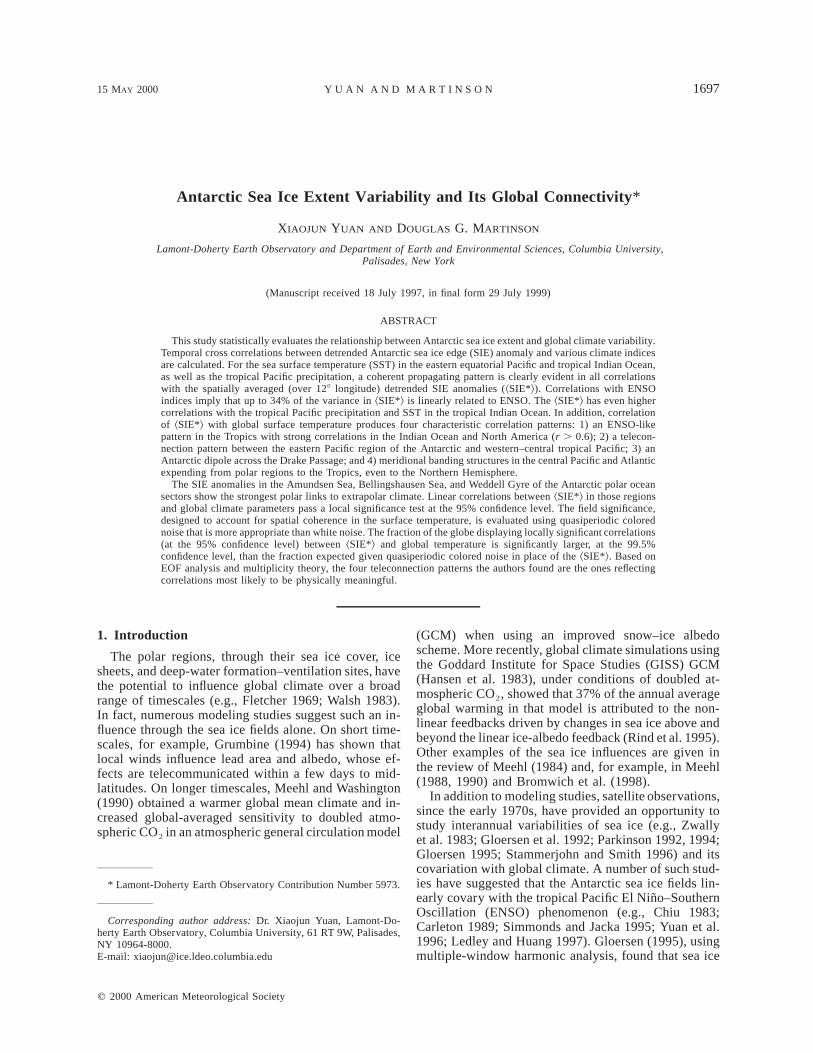
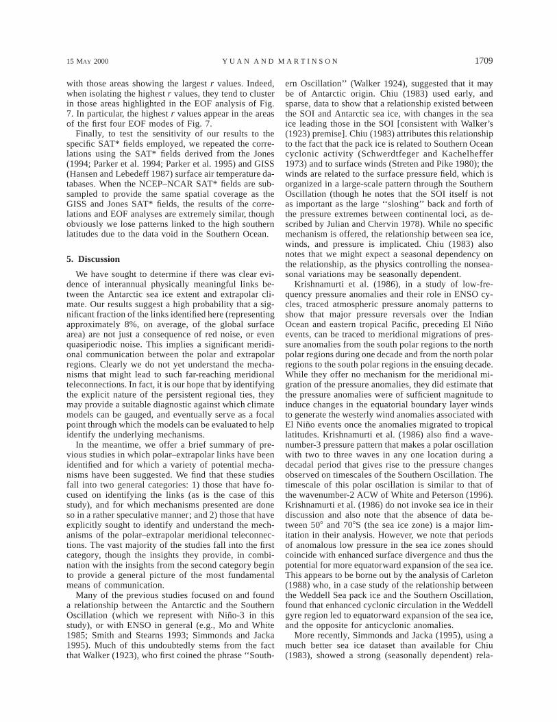
FIG. 1. The linear temporal trend in the SIE9 as a function of longitude (heavy solid line). Dashed lines mark 95% confidence intervalsof the trend. The ice edge shows retreat in the shaded areas and expansion in the open areas. Geographic locations are marked. The easternPacific region mainly includes the Amundsen Sea and Bellingshausen Sea (A and B).

global coverage. When the NCEP–NCAR SAT* field issubsampled to mimic the spatial coverage of the Jones’sand GISS data fields, the principal modes of an empiricalorthogonal function (EOF) analysis (presented below)look similar. More importantly, results of repeating themain correlation analysis of section 4 with the differentSAT* fields are extremely similar.

Other climate parameters used in the study includean ENSO-related index given by Nino-3 (an easternequatorial Pacific sea surface temperature averaged in58N–58S, 1508–908W and robust index for ENSO var-iability; Cane et al. 1986), a Pacific–North American(PNA) teleconnection index, a North Atlantic oscillation(NAO) index, and a Southern Oscillation index (SOI).These climate indices are provided by the NCEP Cli-mate Prediction Center. In addition, we use a tropicalPacific precipitation index based on station data in thearea of 6.258N–6.258S, 163.758E–86.258W and a trop-ical non-Pacific precipitation index based on station datain the area of 208N–208S, 78.758W–163.758E. Both pre-cipitation indices are based on the GISS surface ob-served land precipitation dataset (Dai et al. 1997) andare generated at the University of Washington’s JointInstitute for the Study of the Atmosphere and theOceans. They are available online (http://tao.atmos.washington.edu/datapsets/). Finally, we gen-erate a tropical Indian Ocean sea surface temperature

(SST) index based on Jones’s surface temperature anom-alies in the area of 2.58N–12.58S, 62.58–82.58E. TheIndian Ocean SST has been suggested to be related tomonsoonal intensity (Charles et al. 1997; Kumar 1997).

To focus on interannual (and longer) variability, alltime series were temporally smoothed by a Gaussianfilter with the filter width of 13 months, to remove var-iabilities with periods less than a year.

3. Sea ice edge characteristics

The SIE monthly anomaly series (SIE9), that is, afterremoving the seasonal cycle, contain interannual andlonger variability as well as linear trends. A linear re-gression is applied to the SIE9 as a function of longitudeto capture the trends, which are shown in Fig. 1. Av-eraged around the entire Antarctic continent, the SIE9displays a net increasing trend of 0.011 6 0.0438 yr21,but with a considerable rms noise level of 0.788. Theresult is consistent with the most recent analyses of iceextent trends (Gloersen and Campbell 1991; Weatherlyet al. 1991; Johannessen et al. 1995; Cavalieri et al.1997), though the various studies differ in their assess-ment of the statistical significance (likely a consequenceof the large rms noise which imparts sensitivity to thelength of the record being evaluated).

The spatial heterogeneity apparent in Fig. 1 shows


the average trend to be the net consequence of signif-icant spatial variability. Specifically, the most significantice edge retreat occurs in the Bellingshausen andAmundsen Seas of the eastern Pacific, in agreement withJacobs and Comiso (1997) and Stammerjohn and Smith(1997; which also contains an excellent review of othersea ice trend analyses and possible mechanisms). Con-versely, the ice edge shows equatorward expansion inthe Ross and Weddell Seas, which also agrees withStammerjohn and Smith (1997). For the present study,the trends are removed from the Antarctic SIE9 at eachdegree of latitude, producing a detrended anomaly SIEseries, SIE*.

The spatial decorrelation length of the SIE* field isestimated by calculating the spatial autocorrelation forthe spatial series for each month. The mean decorre-lation length appears as a function of season with amaximum of 178 longitude in February and a minimumof 58 long in August. The former is clearly dominatedby the consistency of the summer SIE. Averaged over12 months, this yields a decorrelation length of 128 lon-gitude. We therefore choose to average the SIE* into128 longitude bands to generate 30 quasi–spatially in-dependent time series, ^SIE*&.

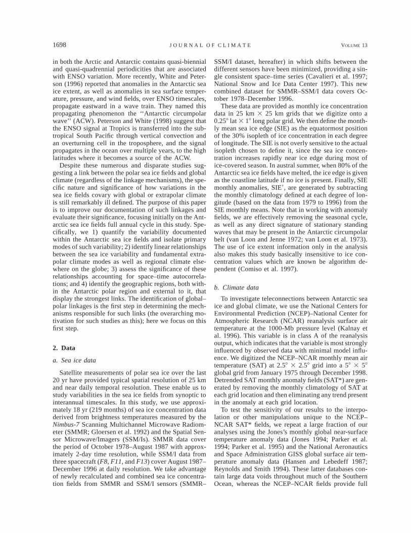
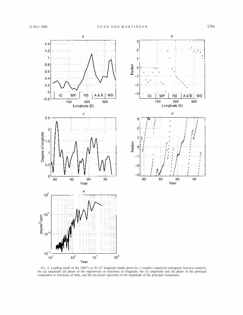
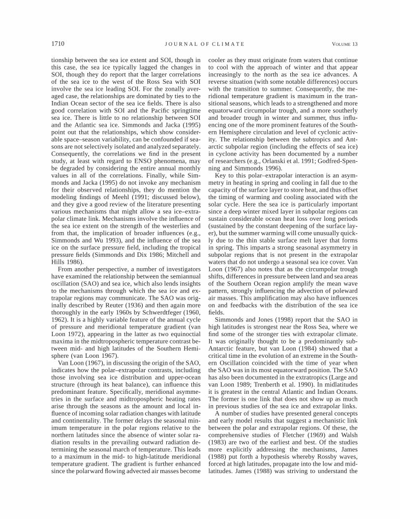
In an attempt to identify coherent spatial–temporalsubstructure in the SIE*, a complex EOF (CEOF) anal-ysis was applied to identify traveling and standingwaves (Wallace and Dickinson 1972; Horel 1984) withinthe SIE* field. The SIE* time series were filtered by aButterworth low-pass filter to eliminate noise with pe-riods less than 1 yr prior to the CEOF analysis. Theleading mode’s spatial pattern (Fig. 2a,b), described byits eigenvector and containing 46% of the total variance,is dominated by two high-variance maxima (of oppositephase): one in the eastern Ross Sea and the other in theWeddell gyre region. The leading mode’s temporal var-iability, as described by its principal component (Fig.2c,d), has a spectrum similar to that of a pure red noisespectrum generated from integrated white noise (Fig.2e). However, the mode does display significant spectralpeaks (95% confidence relative to 100 realizations ofred noise spectra) at frequencies of approximately 1.5–2yr and just over 5-yr periods. Since the gain functionfor the Butterworth filter has a smooth transitional band(Roberts and Roberts 1978), the peak with the 1.5-yrperiod should not be an artifact of the filtering process.

The phase of the first mode eigenvector linearly de-creases eastward (except in the Indian Ocean), and thephase of the principle component linearly increases withtime, which indicates an eastward-propagating signal.This propagating signal is strongest in the region fromthe Ross Sea to the Weddell Sea. The principle com-ponent reveals a dominate variation with a period ofapproximately 5 yr. Analysis of the 5-yr component(Fig. 3) shows that it displays an eastward propagationcomparable to that of the primary mode. This is con-sistent with the general filtered characteristics of theACW (White and Peterson 1996). However, lack of con-

sistent decreasing phase of the eigenvector and rela-tively lower eigenvector magnitude in the Indian Oceansuggest that no clear propagating signal exists there. Thepropagating signal either is limited in the Weddell gyreinstead of continuously propagating into the IndianOcean or becomes too weak to detect east of the Weddellgyre. The analysis cannot differentiate between thesetwo possibilities.

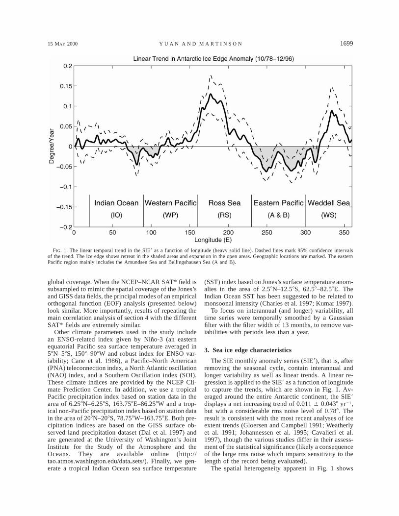
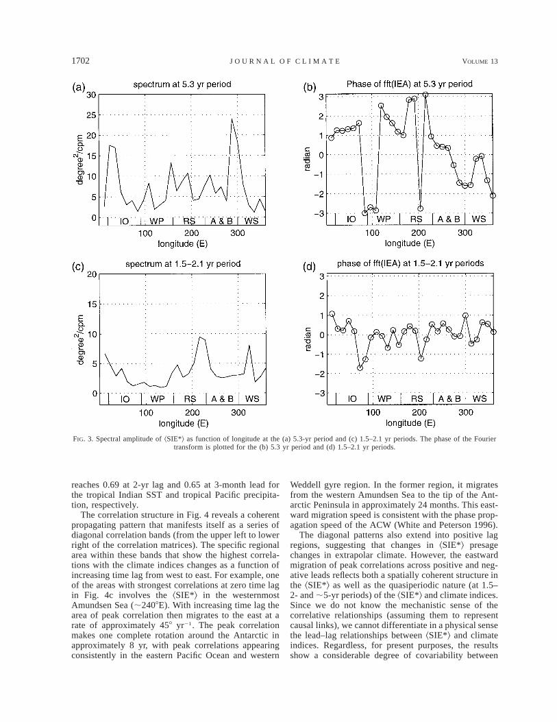
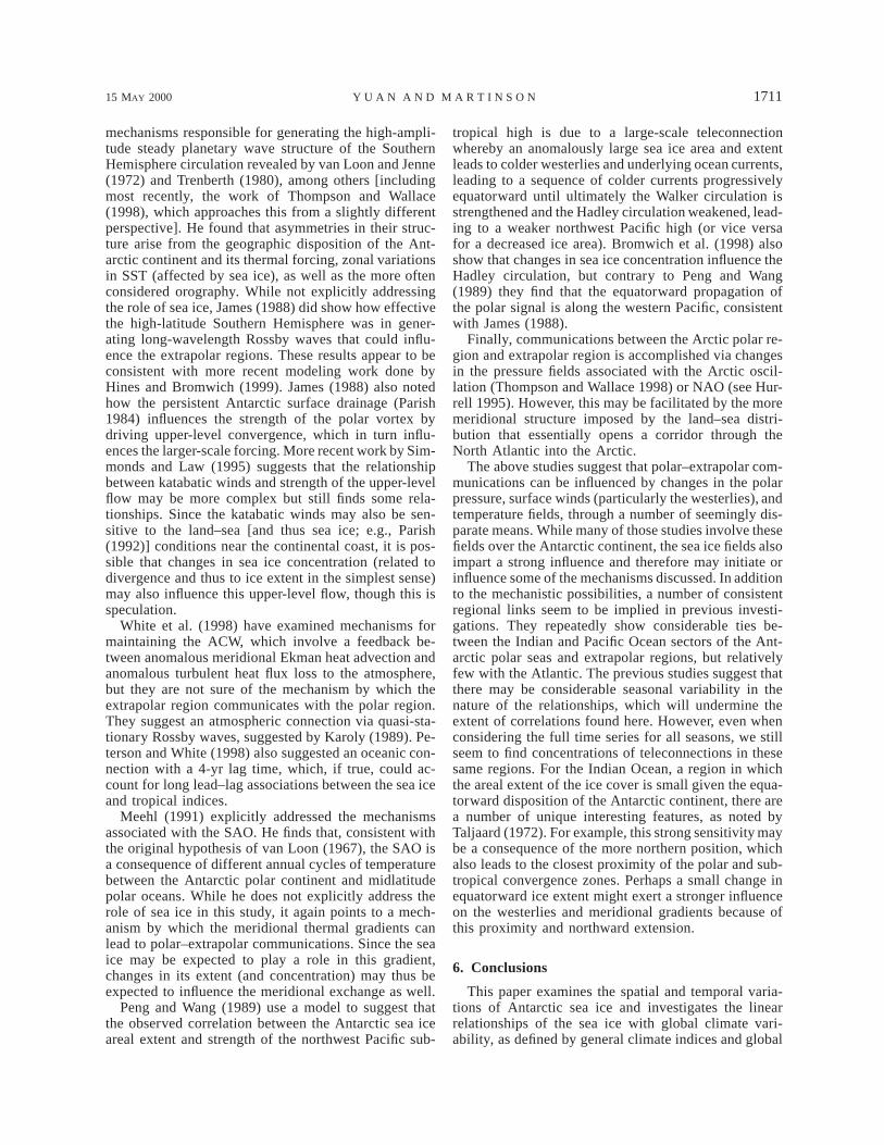
Spectral analysis was also applied to the individualSIE* time series at each 128 longitude band. Peaks withperiods near 1.5–2 and ;5 yr appear in many longitudebands (Fig. 3). The power within the 5-yr period bandis strongest in the western Indian Ocean and central andeastern Pacific. The phase for this band (Fig. 3b) in-dicates an eastward propagation in the Pacific, thoughits flat nature in the western Indian Ocean and westernAmundsen Sea region suggest that the propagation maybe either discontinuous or at different rates in thoseregions. The power for the higher-frequency band (1.5–2.1 yr) is concentrated in the Weddell Sea and east ofthe Ross Sea, although this variability does not appearto propagate spatially. This high-frequency interannualvariability is consistent with the quasi-biennial oscil-lation in the Antarctic ice extent suggested by Gloersen(1995).

The spatial pattern of the second mode (not shown),which contains 16% of the total variance, captures thenonconcentric asymmetry of the Antarctic sea ice fields.That is, the ice shows enhanced variability in the regionsmost equatorward in the central Pacific and westernIndian Ocean. This pattern is particularly strong duringthe period 1987–1989.

4. Global connectivity

a. Tropical climate links

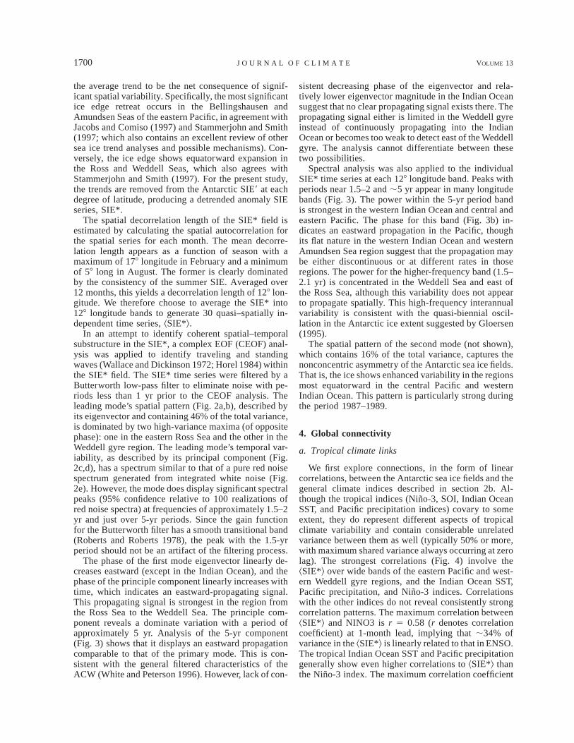
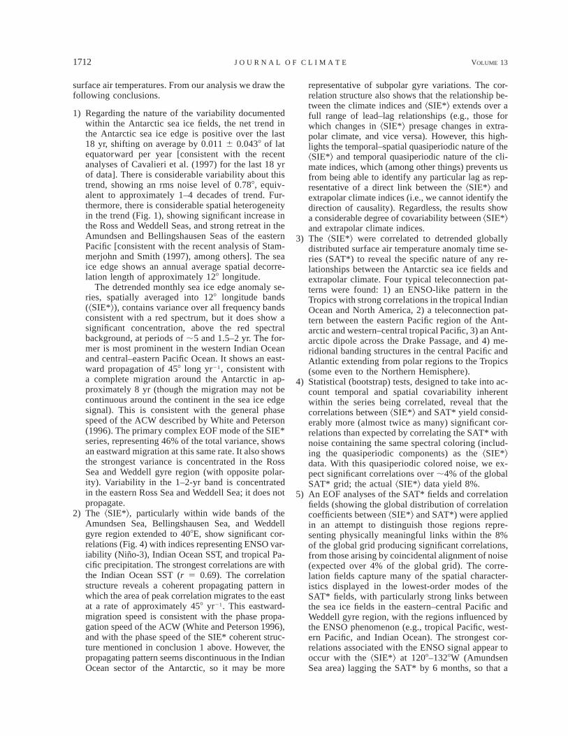
We first explore connections, in the form of linearcorrelations, between the Antarctic sea ice fields and thegeneral climate indices described in section 2b. Al-though the tropical indices (Nino-3, SOI, Indian OceanSST, and Pacific precipitation indices) covary to someextent, they do represent different aspects of tropicalclimate variability and contain considerable unrelatedvariance between them as well (typically 50% or more,with maximum shared variance always occurring at zerolag). The strongest correlations (Fig. 4) involve the^SIE*& over wide bands of the eastern Pacific and west-ern Weddell gyre regions, and the Indian Ocean SST,Pacific precipitation, and Nino-3 indices. Correlationswith the other indices do not reveal consistently strongcorrelation patterns. The maximum correlation between^SIE*& and NINO3 is r 5 0.58 (r denotes correlationcoefficient) at 1-month lead, implying that ;34% ofvariance in the ^SIE*& is linearly related to that in ENSO.The tropical Indian Ocean SST and Pacific precipitationgenerally show even higher correlations to ^SIE*& thanthe Nino-3 index. The maximum correlation coefficient


FIG. 2. Leading mode of the ^SIE*& at 30 128 longitude bands given by a complex empirical orthogonal function analysis:the (a) amplitude (b) phase of the eigenvector as functions of longitude, the (c) amplitude and (d) phase of the principalcomponent as functions of time, and the (e) power spectrum of the amplitude of the principal component.


FIG. 3. Spectral amplitude of ^SIE*& as function of longitude at the (a) 5.3-yr period and (c) 1.5–2.1 yr periods. The phase of the Fouriertransform is plotted for the (b) 5.3 yr period and (d) 1.5–2.1 yr periods.

reaches 0.69 at 2-yr lag and 0.65 at 3-month lead forthe tropical Indian SST and tropical Pacific precipita-tion, respectively.

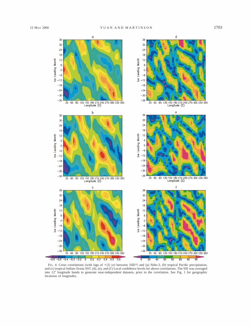
The correlation structure in Fig. 4 reveals a coherentpropagating pattern that manifests itself as a series ofdiagonal correlation bands (from the upper left to lowerright of the correlation matrices). The specific regionalarea within these bands that show the highest correla-tions with the climate indices changes as a function ofincreasing time lag from west to east. For example, oneof the areas with strongest correlations at zero time lagin Fig. 4c involves the ^SIE*& in the westernmostAmundsen Sea (;2408E). With increasing time lag thearea of peak correlation then migrates to the east at arate of approximately 458 yr21. The peak correlationmakes one complete rotation around the Antarctic inapproximately 8 yr, with peak correlations appearingconsistently in the eastern Pacific Ocean and western

Weddell gyre region. In the former region, it migratesfrom the western Amundsen Sea to the tip of the Ant-arctic Peninsula in approximately 24 months. This east-ward migration speed is consistent with the phase prop-agation speed of the ACW (White and Peterson 1996).

The diagonal patterns also extend into positive lagregions, suggesting that changes in ^SIE*& presagechanges in extrapolar climate. However, the eastwardmigration of peak correlations across positive and neg-ative leads reflects both a spatially coherent structure inthe ^SIE*& as well as the quasiperiodic nature (at 1.5–2- and ;5-yr periods) of the ^SIE*& and climate indices.Since we do not know the mechanistic sense of thecorrelative relationships (assuming them to representcausal links), we cannot differentiate in a physical sensethe lead–lag relationships between ^SIE*& and climateindices. Regardless, for present purposes, the resultsshow a considerable degree of covariability between


FIG. 4. Cross correlations (with lags of #|3| yr) between ^SIE*& and (a) Nino-3, (b) tropical Pacific precipitation,and (c) tropical Indian Ocean SST. (d), (e), and (f ) Local confidence levels for above correlations. The SIE was averagedinto 128 longitude bands to generate near-independent datasets, prior to the correlation. See Fig. 1 for geographiclocations of longitudes.


^SIE*& and extrapolar climate indices, and strong spatialcoherency of the relationships with an eastward prop-agation consistent with the phase speed of the ACW.

For the time series used in this analysis, a cross cor-relation of |r| . 0.2 would be significant at 95% con-fidence level if all of the data points in the time serieswere independent. However, the monthly values are notindependent, and their degree of autocorrelation dictatesthat, for most cases, a correlation of |r| . 0.5 is sig-nificant at the 95% confidence level. There are a fewtime series where correlations at the 0.5 level are sig-nificant at just under 95% confidence, and others wherethey are better than 95%, but these are subtle differencesaffecting a minority of series. Also, correlations in-volving the tropical Indian Ocean SST and Pacific pre-cipitation yield slightly higher confidence levels for thesame r value as those involving Nino-3 since the latterhas a higher degree of autocorrelation. All of these fac-tors are taken into account in the confidence levels ofFig. 4. More detailed discussion on the significance testsof these linear correlations is given in the appendix.

b. Links with global surface temperature

While the above correlations suggest that a consid-erable fraction of the variance of the ^SIE*& appears tobe linked to tropical climate variability, as measured bythe climate indices, here we investigate the spatial–tem-poral distribution of polar–global climate links. Initiallythis is done by computing linear correlations betweenthe ^SIE*& and global SAT anomaly series (SAT*) de-scribed in section 2. Since the mean temporal decor-relation length of the ^SIE*& series is about 6 months,the correlations are computed at half-year lag intervalsup to 62 yr, generating a total of 270 global correlationmaps. The confidence level at which the correlation inevery grid cell is significant is calculated using an ef-fective degrees of freedom, as described in the appendix.Since this confidence level only takes into account thetemporal autocorrelation within the ^SIE*& and SAT*series and does not consider spatial coherence withinthe SAT* field, we consider it the ‘‘local’’ confidencelevel. The spatial coherence is tested separately via useof statistical field tests described in the appendix. It isalso considered through EOF analyses later in this sec-tion.

Before attempting to distill physically meaningful re-sults or regional links from the numerous correlations,we first performed a number of tests to assess theirstatistical significance. The tests were designed to de-termine if the results yield more statistically significant(at the 95% confidence level) correlations around theglobe than expected by simply correlating the globalSAT* series to noise displaying the same general spec-tral coloring as the ^SIE*& series. We do this by con-ducting 1) local significance tests that take into accountthe effect of temporal autocorrelations present in thedatasets being correlated, and 2) field significance tests

that take into account the spatial coherence (spanningall scales) inherent in the SAT* data. The details of thesetests and their results are described in the appendix; theyare summarized here for convenience. Finally, we applythe concepts of multiplicity to determine which of thosecorrelations exceeding that expected from simple cor-relations to noise are most likely to represent the phys-ically meaningful ones.

Briefly, the statistical tests show that correlations of^SIE*& with global SAT* reveal considerably more (al-most twice as many) significant correlations than ex-pected by correlating the SAT* with noise containingthe same spectral coloring as the ^SIE*& data. Specifi-cally, on average approximately 4% (mode value) of theglobal grid will yield correlations significant at, orabove, the 95% confidence level if we correlate colorednoise to the SAT*. Instead, using the ^SIE*& data, morethan 8% of the global grid, or twice as much, yieldssignificant correlations on average (i.e., for any partic-ular lag or ^SIE*& series). When comparing means, theresult is more than 9 standard deviations beyond themean expected for the quasiperiodic colored noise. Fur-thermore, there is a large band over which the data showconsiderably more significant correlations than the noiseshows. That is, for significant correlations coveringmore than 6% of the global grid, we find considerablymore (nearly twice as many) results in this band thanwould be expected from correlations with quasiperiodiccolored noise.

Of the correlation fields, 65% of the results yieldinghigher number of significant correlations than expected(at the 95% confidence level) occur for cases in which^SIE*& leads (from 6 to 24 months) changes in SAT*.An additional 13% occurs for zero-lag cases. However,these results are fairly sensitive to subtle changes in thetime series being correlated (e.g., removal of a year ofdata from the ^SIE*& time series changes this result sig-nificantly). These results are also biased somewhat,though not completely, by high southern latitude rela-tionships reflecting a regional influence of ^SIE*& onSAT*; if the SAT* fields south of 508S are removedfrom the correlations, the correlations are more evenlydistributed between positive and negative lags. Conse-quently, we cannot claim any physical significance (atleast outside the Southern Ocean region) to these per-centages at present, and as with the climate indices, thephysical implications of lead–lag relationships in cor-relations are meaningless without a clear understandingof the mechanisms responsible for the links.

Likewise, while the considerable degree of significantcorrelations is a highly robust finding, we cannot dis-tinguish which regions yielding significant correlationsrepresent likely physical links from those that can beexpected to arise from correlations with noise. However,here we can perform additional analyses in an attemptto identify spatial correlation patterns that are consistentwith spatial distributions of known climate phenomena,and therefore likely links to those phenomena. We es-


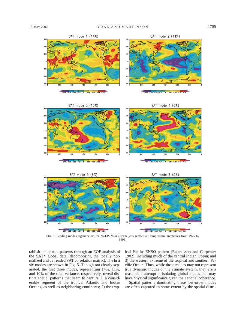
FIG. 5. Leading modes eigenvectors for NCEP–NCAR reanalysis surface air temperature anomalies from 1975 to1998.

tablish the spatial patterns through an EOF analysis ofthe SAT* global data (decomposing the locally nor-malized and detrended SAT correlation matrix). The firstsix modes are shown in Fig. 5. Though not clearly sep-arated, the first three modes, representing 14%, 11%,and 10% of the total variance, respectively, reveal dis-tinct spatial patterns that seem to capture 1) a consid-erable segment of the tropical Atlantic and IndianOceans, as well as neighboring continents; 2) the trop-

ical Pacific ENSO pattern (Rasmusson and Carpenter1982), including much of the central Indian Ocean; and3) the western extreme of the tropical and southern Pa-cific Ocean. Thus, while these modes may not representtrue dynamic modes of the climate system, they are areasonable attempt at isolating global modes that mayhave physical significance given their spatial coherence.

Spatial patterns dominating these low-order modesare often captured to some extent by the spatial distri-


bution of significant correlations, as seen in the corre-lation maps. For example, four correlation maps, pre-sented with their local significance (see appendix forstatistical assessments), are presented in Fig. 6. Thesehighlight the principal patterns that recur throughout thecorrelations, and which are often present to some degreein the modes.

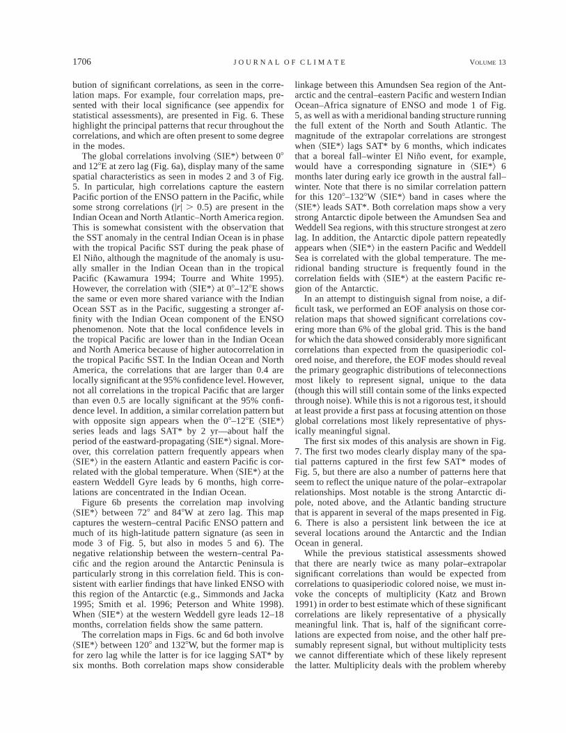
The global correlations involving ^SIE*& between 08and 128E at zero lag (Fig. 6a), display many of the samespatial characteristics as seen in modes 2 and 3 of Fig.5. In particular, high correlations capture the easternPacific portion of the ENSO pattern in the Pacific, whilesome strong correlations (|r| . 0.5) are present in theIndian Ocean and North Atlantic–North America region.This is somewhat consistent with the observation thatthe SST anomaly in the central Indian Ocean is in phasewith the tropical Pacific SST during the peak phase ofEl Nino, although the magnitude of the anomaly is usu-ally smaller in the Indian Ocean than in the tropicalPacific (Kawamura 1994; Tourre and White 1995).However, the correlation with ^SIE*& at 08–128E showsthe same or even more shared variance with the IndianOcean SST as in the Pacific, suggesting a stronger af-finity with the Indian Ocean component of the ENSOphenomenon. Note that the local confidence levels inthe tropical Pacific are lower than in the Indian Oceanand North America because of higher autocorrelation inthe tropical Pacific SST. In the Indian Ocean and NorthAmerica, the correlations that are larger than 0.4 arelocally significant at the 95% confidence level. However,not all correlations in the tropical Pacific that are largerthan even 0.5 are locally significant at the 95% confi-dence level. In addition, a similar correlation pattern butwith opposite sign appears when the 08–128E ^SIE*&series leads and lags SAT* by 2 yr—about half theperiod of the eastward-propagating ^SIE*& signal. More-over, this correlation pattern frequently appears when^SIE*& in the eastern Atlantic and eastern Pacific is cor-related with the global temperature. When ^SIE*& at theeastern Weddell Gyre leads by 6 months, high corre-lations are concentrated in the Indian Ocean.

Figure 6b presents the correlation map involving^SIE*& between 728 and 848W at zero lag. This mapcaptures the western–central Pacific ENSO pattern andmuch of its high-latitude pattern signature (as seen inmode 3 of Fig. 5, but also in modes 5 and 6). Thenegative relationship between the western–central Pa-cific and the region around the Antarctic Peninsula isparticularly strong in this correlation field. This is con-sistent with earlier findings that have linked ENSO withthis region of the Antarctic (e.g., Simmonds and Jacka1995; Smith et al. 1996; Peterson and White 1998).When ^SIE*& at the western Weddell gyre leads 12–18months, correlation fields show the same pattern.

The correlation maps in Figs. 6c and 6d both involve^SIE*& between 1208 and 1328W, but the former map isfor zero lag while the latter is for ice lagging SAT* bysix months. Both correlation maps show considerable

linkage between this Amundsen Sea region of the Ant-arctic and the central–eastern Pacific and western IndianOcean–Africa signature of ENSO and mode 1 of Fig.5, as well as with a meridional banding structure runningthe full extent of the North and South Atlantic. Themagnitude of the extrapolar correlations are strongestwhen ^SIE*& lags SAT* by 6 months, which indicatesthat a boreal fall–winter El Nino event, for example,would have a corresponding signature in ^SIE*& 6months later during early ice growth in the austral fall–winter. Note that there is no similar correlation patternfor this 1208–1328W ^SIE*& band in cases where the^SIE*& leads SAT*. Both correlation maps show a verystrong Antarctic dipole between the Amundsen Sea andWeddell Sea regions, with this structure strongest at zerolag. In addition, the Antarctic dipole pattern repeatedlyappears when ^SIE*& in the eastern Pacific and WeddellSea is correlated with the global temperature. The me-ridional banding structure is frequently found in thecorrelation fields with ^SIE*& at the eastern Pacific re-gion of the Antarctic.

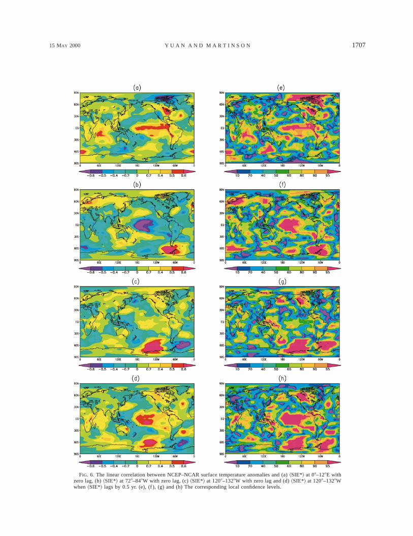
In an attempt to distinguish signal from noise, a dif-ficult task, we performed an EOF analysis on those cor-relation maps that showed significant correlations cov-ering more than 6% of the global grid. This is the bandfor which the data showed considerably more significantcorrelations than expected from the quasiperiodic col-ored noise, and therefore, the EOF modes should revealthe primary geographic distributions of teleconnectionsmost likely to represent signal, unique to the data(though this will still contain some of the links expectedthrough noise). While this is not a rigorous test, it shouldat least provide a first pass at focusing attention on thoseglobal correlations most likely representative of phys-ically meaningful signal.

The first six modes of this analysis are shown in Fig.7. The first two modes clearly display many of the spa-tial patterns captured in the first few SAT* modes ofFig. 5, but there are also a number of patterns here thatseem to reflect the unique nature of the polar–extrapolarrelationships. Most notable is the strong Antarctic di-pole, noted above, and the Atlantic banding structurethat is apparent in several of the maps presented in Fig.6. There is also a persistent link between the ice atseveral locations around the Antarctic and the IndianOcean in general.

While the previous statistical assessments showedthat there are nearly twice as many polar–extrapolarsignificant correlations than would be expected fromcorrelations to quasiperiodic colored noise, we must in-voke the concepts of multiplicity (Katz and Brown1991) in order to best estimate which of these significantcorrelations are likely representative of a physicallymeaningful link. That is, half of the significant corre-lations are expected from noise, and the other half pre-sumably represent signal, but without multiplicity testswe cannot differentiate which of these likely representthe latter. Multiplicity deals with the problem whereby


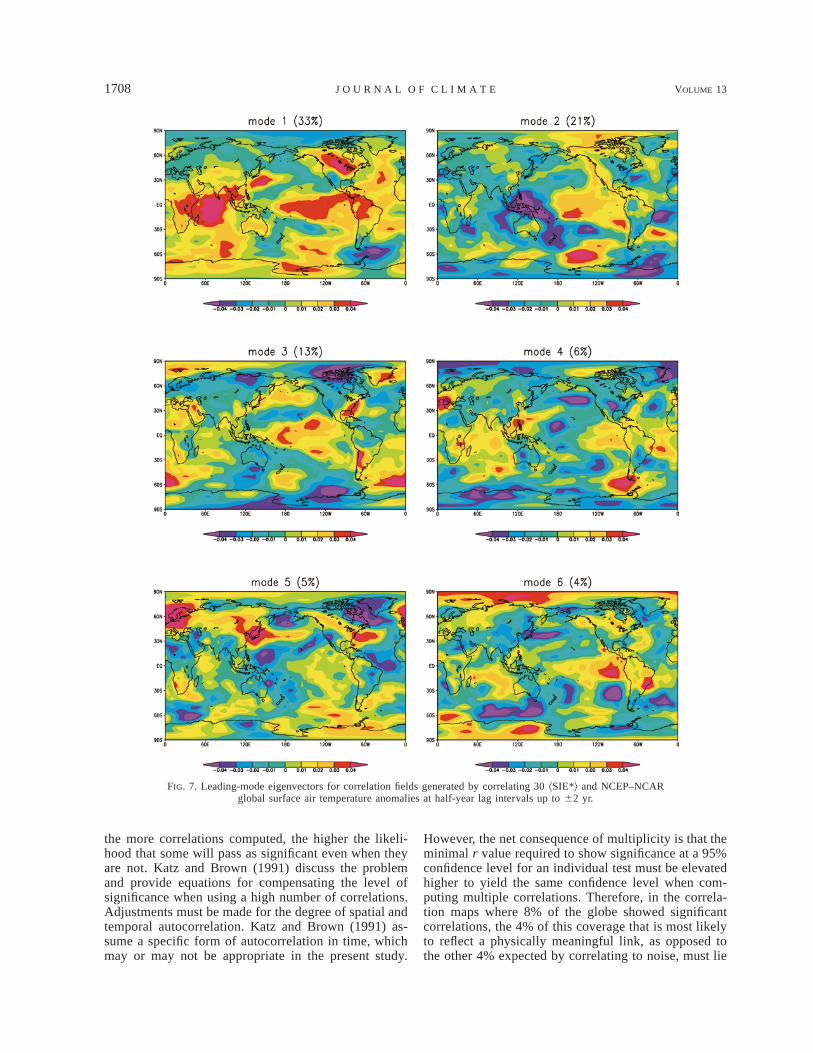
FIG. 6. The linear correlation between NCEP–NCAR surface temperature anomalies and (a) ^SIE*& at 08–128E withzero lag, (b) ^SIE*& at 728–848W with zero lag, (c) ^SIE*& at 1208–1328W with zero lag and (d) ^SIE*& at 1208–1328Wwhen ^SIE*& lags by 0.5 yr. (e), (f ), (g) and (h) The corresponding local confidence levels.


FIG. 7. Leading-mode eigenvectors for correlation fields generated by correlating 30 ^SIE*& and NCEP–NCARglobal surface air temperature anomalies at half-year lag intervals up to 62 yr.

the more correlations computed, the higher the likeli-hood that some will pass as significant even when theyare not. Katz and Brown (1991) discuss the problemand provide equations for compensating the level ofsignificance when using a high number of correlations.Adjustments must be made for the degree of spatial andtemporal autocorrelation. Katz and Brown (1991) as-sume a specific form of autocorrelation in time, whichmay or may not be appropriate in the present study.

However, the net consequence of multiplicity is that theminimal r value required to show significance at a 95%confidence level for an individual test must be elevatedhigher to yield the same confidence level when com-puting multiple correlations. Therefore, in the correla-tion maps where 8% of the globe showed significantcorrelations, the 4% of this coverage that is most likelyto reflect a physically meaningful link, as opposed tothe other 4% expected by correlating to noise, must lie


with those areas showing the largest r values. Indeed,when isolating the highest r values, they tend to clusterin those areas highlighted in the EOF analysis of Fig.7. In particular, the highest r values appear in the areasof the first four EOF modes of Fig. 7.

Finally, to test the sensitivity of our results to thespecific SAT* fields employed, we repeated the corre-lations using the SAT* fields derived from the Jones(1994; Parker et al. 1994; Parker et al. 1995) and GISS(Hansen and Lebedeff 1987) surface air temperature da-tabases. When the NCEP–NCAR SAT* fields are sub-sampled to provide the same spatial coverage as theGISS and Jones SAT* fields, the results of the corre-lations and EOF analyses are extremely similar, thoughobviously we lose patterns linked to the high southernlatitudes due to the data void in the Southern Ocean.

5. Discussion

We have sought to determine if there was clear evi-dence of interannual physically meaningful links be-tween the Antarctic sea ice extent and extrapolar cli-mate. Our results suggest a high probability that a sig-nificant fraction of the links identified here (representingapproximately 8%, on average, of the global surfacearea) are not just a consequence of red noise, or evenquasiperiodic noise. This implies a significant meridi-onal communication between the polar and extrapolarregions. Clearly we do not yet understand the mecha-nisms that might lead to such far-reaching meridionalteleconnections. In fact, it is our hope that by identifyingthe explicit nature of the persistent regional ties, theymay provide a suitable diagnostic against which climatemodels can be gauged, and eventually serve as a focalpoint through which the models can be evaluated to helpidentify the underlying mechanisms.

In the meantime, we offer a brief summary of pre-vious studies in which polar–extrapolar links have beenidentified and for which a variety of potential mecha-nisms have been suggested. We find that these studiesfall into two general categories: 1) those that have fo-cused on identifying the links (as is the case of thisstudy), and for which mechanisms presented are doneso in a rather speculative manner; and 2) those that haveexplicitly sought to identify and understand the mech-anisms of the polar–extrapolar meridional teleconnec-tions. The vast majority of the studies fall into the firstcategory, though the insights they provide, in combi-nation with the insights from the second category beginto provide a general picture of the most fundamentalmeans of communication.

Many of the previous studies focused on and founda relationship between the Antarctic and the SouthernOscillation (which we represent with Nino-3 in thisstudy), or with ENSO in general (e.g., Mo and White1985; Smith and Stearns 1993; Simmonds and Jacka1995). Much of this undoubtedly stems from the factthat Walker (1923), who first coined the phrase ‘‘South-

ern Oscillation’’ (Walker 1924), suggested that it maybe of Antarctic origin. Chiu (1983) used early, andsparse, data to show that a relationship existed betweenthe SOI and Antarctic sea ice, with changes in the seaice leading those in the SOI [consistent with Walker’s(1923) premise]. Chiu (1983) attributes this relationshipto the fact that the pack ice is related to Southern Oceancyclonic activity (Schwerdtfeger and Kachelheffer1973) and to surface winds (Streten and Pike 1980); thewinds are related to the surface pressure field, which isorganized in a large-scale pattern through the SouthernOscillation (though he notes that the SOI itself is notas important as the large ‘‘sloshing’’ back and forth ofthe pressure extremes between continental loci, as de-scribed by Julian and Chervin 1978). While no specificmechanism is offered, the relationship between sea ice,winds, and pressure is implicated. Chiu (1983) alsonotes that we might expect a seasonal dependency onthe relationship, as the physics controlling the nonsea-sonal variations may be seasonally dependent.

Krishnamurti et al. (1986), in a study of low-fre-quency pressure anomalies and their role in ENSO cy-cles, traced atmospheric pressure anomaly patterns toshow that major pressure reversals over the IndianOcean and eastern tropical Pacific, preceding El Ninoevents, can be traced to meridional migrations of pres-sure anomalies from the south polar regions to the northpolar regions during one decade and from the north polarregions to the south polar regions in the ensuing decade.While they offer no mechanism for the meridional mi-gration of the pressure anomalies, they did estimate thatthe pressure anomalies were of sufficient magnitude toinduce changes in the equatorial boundary layer windsto generate the westerly wind anomalies associated withEl Nino events once the anomalies migrated to tropicallatitudes. Krishnamurti et al. (1986) also find a wave-number-3 pressure pattern that makes a polar oscillationwith two to three waves in any one location during adecadal period that gives rise to the pressure changesobserved on timescales of the Southern Oscillation. Thetimescale of this polar oscillation is similar to that ofthe wavenumber-2 ACW of White and Peterson (1996).Krishnamurti et al. (1986) do not invoke sea ice in theirdiscussion and also note that the absence of data be-tween 508 and 708S (the sea ice zone) is a major lim-itation in their analysis. However, we note that periodsof anomalous low pressure in the sea ice zones shouldcoincide with enhanced surface divergence and thus thepotential for more equatorward expansion of the sea ice.This appears to be borne out by the analysis of Carleton(1988) who, in a case study of the relationship betweenthe Weddell Sea pack ice and the Southern Oscillation,found that enhanced cyclonic circulation in the Weddellgyre region led to equatorward expansion of the sea ice,and the opposite for anticyclonic anomalies.

More recently, Simmonds and Jacka (1995), using amuch better sea ice dataset than available for Chiu(1983), showed a strong (seasonally dependent) rela-


tionship between the sea ice extent and SOI, though inthis case, the sea ice typically lagged the changes inSOI, though they do report that the larger correlationsof the sea ice to the west of the Ross Sea with SOIinvolve the sea ice leading SOI. For the zonally aver-aged case, the relationships are dominated by ties to theIndian Ocean sector of the sea ice fields. There is alsogood correlation with SOI and the Pacific springtimesea ice. There is little to no relationship between SOIand the Atlantic sea ice. Simmonds and Jacka (1995)point out that the relationships, which show consider-able space–season variability, can be confounded if sea-sons are not selectively isolated and analyzed separately.Consequently, the correlations we find in the presentstudy, at least with regard to ENSO phenomena, maybe degraded by considering the entire annual monthlyvalues in all of the correlations. Finally, while Sim-monds and Jacka (1995) do not invoke any mechanismfor their observed relationships, they do mention themodeling findings of Meehl (1991; discussed below),and they give a good review of the literature presentingvarious mechanisms that might allow a sea ice–extra-polar climate link. Mechanisms involve the influence ofthe sea ice extent on the strength of the westerlies andfrom that, the implication of broader influences (e.g.,Simmonds and Wu 1993), and the influence of the seaice on the surface pressure field, including the tropicalpressure fields (Simmonds and Dix 1986; Mitchell andHills 1986).

From another perspective, a number of investigatorshave examined the relationship between the semiannualoscillation (SAO) and sea ice, which also lends insightsto the mechanisms through which the sea ice and ex-trapolar regions may communicate. The SAO was orig-inally described by Reuter (1936) and then again morethoroughly in the early 1960s by Schwerdtfeger (1960,1962). It is a highly variable feature of the annual cycleof pressure and meridional temperature gradient (vanLoon 1972), appearing in the latter as two equinoctialmaxima in the midtropospheric temperature contrast be-tween mid- and high latitudes of the Southern Hemi-sphere (van Loon 1967).

Van Loon (1967), in discussing the origin of the SAO,indicates how the polar–extrapolar contrasts, includingthose involving sea ice distribution and upper-oceanstructure (through its heat balance), can influence thispredominant feature. Specifically, meridional asymme-tries in the surface and midtropospheric heating ratesarise through the seasons as the amount and local in-fluence of incoming solar radiation changes with latitudeand continentality. The former delays the seasonal min-imum temperature in the polar regions relative to thenorthern latitudes since the absence of winter solar ra-diation results in the prevailing outward radiation de-termining the seasonal march of temperature. This leadsto a maximum in the mid- to high-latitude meridionaltemperature gradient. The gradient is further enhancedsince the polarward flowing advected air masses become

cooler as they must originate from waters that continueto cool with the approach of winter and that appearincreasingly to the north as the sea ice advances. Areverse situation (with some notable differences) occurswith the transition to summer. Consequently, the me-ridional temperature gradient is maximum in the tran-sitional seasons, which leads to a strengthened and moreequatorward circumpolar trough, and a more southerlyand broader trough in winter and summer, thus influ-encing one of the more prominent features of the South-ern Hemisphere circulation and level of cyclonic activ-ity. The relationship between the subtropics and Ant-arctic subpolar region (including the effects of sea ice)in cyclone activity has been documented by a numberof researchers (e.g., Orlanski et al. 1991; Godfred-Spen-ning and Simmonds 1996).

Key to this polar–extrapolar interaction is an asym-metry in heating in spring and cooling in fall due to thecapacity of the surface layer to store heat, and thus offsetthe timing of warming and cooling associated with thesolar cycle. Here the sea ice is particularly importantsince a deep winter mixed layer in subpolar regions cansustain considerable ocean heat loss over long periods(sustained by the constant deepening of the surface lay-er), but the summer warming will come unusually quick-ly due to the thin stable surface melt layer that formsin spring. This imparts a strong seasonal asymmetry insubpolar regions that is not present in the extrapolarwaters that do not undergo a seasonal sea ice cover. VanLoon (1967) also notes that as the circumpolar troughshifts, differences in pressure between land and sea areasof the Southern Ocean region amplify the mean wavepattern, strongly influencing the advection of polewardair masses. This amplification may also have influenceson and feedbacks with the distribution of the sea icefields.

Simmonds and Jones (1998) report that the SAO inhigh latitudes is strongest near the Ross Sea, where wefind some of the stronger ties with extrapolar climate.It was originally thought to be a predominantly sub-Antarctic feature, but van Loon (1984) showed that acritical time in the evolution of an extreme in the South-ern Oscillation coincided with the time of year whenthe SAO was in its most equatorward position. The SAOhas also been documented in the extratropics (Large andvan Loon 1989; Trenberth et al. 1990). In midlatitudesit is greatest in the central Atlantic and Indian Oceans.The former is one link that does not show up as muchin previous studies of the sea ice and extrapolar links.

A number of studies have presented general conceptsand early model results that suggest a mechanistic linkbetween the polar and extrapolar regions. Of these, thecomprehensive studies of Fletcher (1969) and Walsh(1983) are two of the earliest and best. Of the studiesmore explicitly addressing the mechanisms, James(1988) put forth a hypothesis whereby Rossby waves,forced at high latitudes, propagate into the low and mid-latitudes. James (1988) was striving to understand the


mechanisms responsible for generating the high-ampli-tude steady planetary wave structure of the SouthernHemisphere circulation revealed by van Loon and Jenne(1972) and Trenberth (1980), among others [includingmost recently, the work of Thompson and Wallace(1998), which approaches this from a slightly differentperspective]. He found that asymmetries in their struc-ture arise from the geographic disposition of the Ant-arctic continent and its thermal forcing, zonal variationsin SST (affected by sea ice), as well as the more oftenconsidered orography. While not explicitly addressingthe role of sea ice, James (1988) did show how effectivethe high-latitude Southern Hemisphere was in gener-ating long-wavelength Rossby waves that could influ-ence the extrapolar regions. These results appear to beconsistent with more recent modeling work done byHines and Bromwich (1999). James (1988) also notedhow the persistent Antarctic surface drainage (Parish1984) influences the strength of the polar vortex bydriving upper-level convergence, which in turn influ-ences the larger-scale forcing. More recent work by Sim-monds and Law (1995) suggests that the relationshipbetween katabatic winds and strength of the upper-levelflow may be more complex but still finds some rela-tionships. Since the katabatic winds may also be sen-sitive to the land–sea [and thus sea ice; e.g., Parish(1992)] conditions near the continental coast, it is pos-sible that changes in sea ice concentration (related todivergence and thus to ice extent in the simplest sense)may also influence this upper-level flow, though this isspeculation.

White et al. (1998) have examined mechanisms formaintaining the ACW, which involve a feedback be-tween anomalous meridional Ekman heat advection andanomalous turbulent heat flux loss to the atmosphere,but they are not sure of the mechanism by which theextrapolar region communicates with the polar region.They suggest an atmospheric connection via quasi-sta-tionary Rossby waves, suggested by Karoly (1989). Pe-terson and White (1998) also suggested an oceanic con-nection with a 4-yr lag time, which, if true, could ac-count for long lead–lag associations between the sea iceand tropical indices.

Meehl (1991) explicitly addressed the mechanismsassociated with the SAO. He finds that, consistent withthe original hypothesis of van Loon (1967), the SAO isa consequence of different annual cycles of temperaturebetween the Antarctic polar continent and midlatitudepolar oceans. While he does not explicitly address therole of sea ice in this study, it again points to a mech-anism by which the meridional thermal gradients canlead to polar–extrapolar communications. Since the seaice may be expected to play a role in this gradient,changes in its extent (and concentration) may thus beexpected to influence the meridional exchange as well.

Peng and Wang (1989) use a model to suggest thatthe observed correlation between the Antarctic sea iceareal extent and strength of the northwest Pacific sub-

tropical high is due to a large-scale teleconnectionwhereby an anomalously large sea ice area and extentleads to colder westerlies and underlying ocean currents,leading to a sequence of colder currents progressivelyequatorward until ultimately the Walker circulation isstrengthened and the Hadley circulation weakened, lead-ing to a weaker northwest Pacific high (or vice versafor a decreased ice area). Bromwich et al. (1998) alsoshow that changes in sea ice concentration influence theHadley circulation, but contrary to Peng and Wang(1989) they find that the equatorward propagation ofthe polar signal is along the western Pacific, consistentwith James (1988).

Finally, communications between the Arctic polar re-gion and extrapolar region is accomplished via changesin the pressure fields associated with the Arctic oscil-lation (Thompson and Wallace 1998) or NAO (see Hur-rell 1995). However, this may be facilitated by the moremeridional structure imposed by the land–sea distri-bution that essentially opens a corridor through theNorth Atlantic into the Arctic.

The above studies suggest that polar–extrapolar com-munications can be influenced by changes in the polarpressure, surface winds (particularly the westerlies), andtemperature fields, through a number of seemingly dis-parate means. While many of those studies involve thesefields over the Antarctic continent, the sea ice fields alsoimpart a strong influence and therefore may initiate orinfluence some of the mechanisms discussed. In additionto the mechanistic possibilities, a number of consistentregional links seem to be implied in previous investi-gations. They repeatedly show considerable ties be-tween the Indian and Pacific Ocean sectors of the Ant-arctic polar seas and extrapolar regions, but relativelyfew with the Atlantic. The previous studies suggest thatthere may be considerable seasonal variability in thenature of the relationships, which will undermine theextent of correlations found here. However, even whenconsidering the full time series for all seasons, we stillseem to find concentrations of teleconnections in thesesame regions. For the Indian Ocean, a region in whichthe areal extent of the ice cover is small given the equa-torward disposition of the Antarctic continent, there area number of unique interesting features, as noted byTaljaard (1972). For example, this strong sensitivity maybe a consequence of the more northern position, whichalso leads to the closest proximity of the polar and sub-tropical convergence zones. Perhaps a small change inequatorward ice extent might exert a stronger influenceon the westerlies and meridional gradients because ofthis proximity and northward extension.

6. Conclusions

This paper examines the spatial and temporal varia-tions of Antarctic sea ice and investigates the linearrelationships of the sea ice with global climate vari-ability, as defined by general climate indices and global


surface air temperatures. From our analysis we draw thefollowing conclusions.

1) Regarding the nature of the variability documentedwithin the Antarctic sea ice fields, the net trend inthe Antarctic sea ice edge is positive over the last18 yr, shifting on average by 0.011 6 0.0438 of latequatorward per year [consistent with the recentanalyses of Cavalieri et al. (1997) for the last 18 yrof data]. There is considerable variability about thistrend, showing an rms noise level of 0.788, equiv-alent to approximately 1–4 decades of trend. Fur-thermore, there is considerable spatial heterogeneityin the trend (Fig. 1), showing significant increase inthe Ross and Weddell Seas, and strong retreat in theAmundsen and Bellingshausen Seas of the easternPacific [consistent with the recent analysis of Stam-merjohn and Smith (1997), among others]. The seaice edge shows an annual average spatial decorre-lation length of approximately 128 longitude.

The detrended monthly sea ice edge anomaly se-ries, spatially averaged into 128 longitude bands(^SIE*&), contains variance over all frequency bandsconsistent with a red spectrum, but it does show asignificant concentration, above the red spectralbackground, at periods of ;5 and 1.5–2 yr. The for-mer is most prominent in the western Indian Oceanand central–eastern Pacific Ocean. It shows an east-ward propagation of 458 long yr21, consistent witha complete migration around the Antarctic in ap-proximately 8 yr (though the migration may not becontinuous around the continent in the sea ice edgesignal). This is consistent with the general phasespeed of the ACW described by White and Peterson(1996). The primary complex EOF mode of the SIE*series, representing 46% of the total variance, showsan eastward migration at this same rate. It also showsthe strongest variance is concentrated in the RossSea and Weddell gyre region (with opposite polar-ity). Variability in the 1–2-yr band is concentratedin the eastern Ross Sea and Weddell Sea; it does notpropagate.

2) The ^SIE*&, particularly within wide bands of theAmundsen Sea, Bellingshausen Sea, and Weddellgyre region extended to 408E, show significant cor-relations (Fig. 4) with indices representing ENSO var-iability (Nino-3), Indian Ocean SST, and tropical Pa-cific precipitation. The strongest correlations are withthe Indian Ocean SST (r 5 0.69). The correlationstructure reveals a coherent propagating pattern inwhich the area of peak correlation migrates to the eastat a rate of approximately 458 yr21. This eastward-migration speed is consistent with the phase propa-gation speed of the ACW (White and Peterson 1996),and with the phase speed of the SIE* coherent struc-ture mentioned in conclusion 1 above. However, thepropagating pattern seems discontinuous in the IndianOcean sector of the Antarctic, so it may be more

representative of subpolar gyre variations. The cor-relation structure also shows that the relationship be-tween the climate indices and ^SIE*& extends over afull range of lead–lag relationships (e.g., those forwhich changes in ^SIE*& presage changes in extra-polar climate, and vice versa). However, this high-lights the temporal–spatial quasiperiodic nature of the^SIE*& and temporal quasiperiodic nature of the cli-mate indices, which (among other things) prevents usfrom being able to identify any particular lag as rep-resentative of a direct link between the ^SIE*& andextrapolar climate indices (i.e., we cannot identify thedirection of causality). Regardless, the results showa considerable degree of covariability between ^SIE*&and extrapolar climate indices.

3) The ^SIE*& were correlated to detrended globallydistributed surface air temperature anomaly time se-ries (SAT*) to reveal the specific nature of any re-lationships between the Antarctic sea ice fields andextrapolar climate. Four typical teleconnection pat-terns were found: 1) an ENSO-like pattern in theTropics with strong correlations in the tropical IndianOcean and North America, 2) a teleconnection pat-tern between the eastern Pacific region of the Ant-arctic and western–central tropical Pacific, 3) an Ant-arctic dipole across the Drake Passage, and 4) me-ridional banding structures in the central Pacific andAtlantic extending from polar regions to the Tropics(some even to the Northern Hemisphere).

4) Statistical (bootstrap) tests, designed to take into ac-count temporal and spatial covariability inherentwithin the series being correlated, reveal that thecorrelations between ^SIE*& and SAT* yield consid-erably more (almost twice as many) significant cor-relations than expected by correlating the SAT* withnoise containing the same spectral coloring (includ-ing the quasiperiodic components) as the ^SIE*&data. With this quasiperiodic colored noise, we ex-pect significant correlations over ;4% of the globalSAT* grid; the actual ^SIE*& data yield 8%.

5) An EOF analyses of the SAT* fields and correlationfields (showing the global distribution of correlationcoefficients between ^SIE*& and SAT*) were appliedin an attempt to distinguish those regions repre-senting physically meaningful links within the 8%of the global grid producing significant correlations,from those arising by coincidental alignment of noise(expected over 4% of the global grid). The corre-lation fields capture many of the spatial character-istics displayed in the lowest-order modes of theSAT* fields, with particularly strong links betweenthe sea ice fields in the eastern–central Pacific andWeddell gyre region, with the regions influenced bythe ENSO phenomenon (e.g., tropical Pacific, west-ern Pacific, and Indian Ocean). The strongest cor-relations associated with the ENSO signal appear tooccur with the ^SIE*& at 1208–1328W (AmundsenSea area) lagging the SAT* by 6 months, so that a


boreal fall–winter El Nino event, for example, wouldhave a corresponding signature in ^SIE*& 6 monthslater during early ice growth in the austral fall–win-ter. This region of the Antarctic also links with ameridional banding structure running the full extentof the North and South Atlantic.

In addition, the EOF decomposition of the cor-relation fields, concentrating on those maps forwhich the spatial area of significant correlations (atthe 95% confidence level) exceeds that expected inthe quasiperiodic colored noise, displays many ofthe spatial patterns captured in the first few SAT*modes (e.g., ENSO), as well as a number of patternsthat seem to reflect the unique nature of the polar–extrapolar relationships. Most notable is a strongAntarctic dipole, between the eastern Pacific andwestern Weddell, and the Atlantic banding structurementioned above. There is also a persistent link be-tween the ice at several locations around the Ant-arctic and the Indian Ocean.

We compare the spatial distribution of significantcorrelations to the patterns dominating the SAT*EOF modes to see what fraction of significant cor-relations coincides with these regions. For the casesexamined (those of Fig. 6), 50%–70% of the sig-nificant area overlaps with the highest-amplitudeportions of the modes. This is consistent with aninterpretation that significant correlations within re-gions representing the principal climate patterns, orsome fraction of them, are likely to be physicallymeaningful, while the fraction of significant corre-lations lying outside of these regions arises fromcoincidental alignment of noise. This interpretationshould eventually be tested against models that havea demonstrated ability for simulating observed glob-al climate teleconnections.

Acknowledgments. The authors thank Drs. Y. Kushnir,D. J. Cavalieri, and S. Jacobs for their helpful discussionsand comments. We are especially grateful to Dr. D. J.Cavalieri for providing additional sea ice data. BothSMMR–SSM/I and SSM/I F13 sea ice concentration datawere provided by National Snow and Ice Data Center(NSIDC). Digital data are available from NSIDC distrib-uted Active Archive Center ([email protected]),University of Colorado at Boulder, Boulder, Colorado.This research was supported in part by Lamont-DohertyEarth Observatory seed money and in part by an envi-ronmental research gift from the Ford Motor Company.

APPENDIX

Significance Test for Linear Correlations

a. Local (temporal) significance test

The temporal autocorrelation, or serial correlation,that must be accounted for in the local test (for the

correlations in both sections 4a and 4b) implies that thedata points within the time series being correlated arenot independent. We must thus apply a technique toestimate the number of independent samples in eachtime series, or the effective degrees of freedom (EDOF).We employ a technique modified from Davis (1976) andused in many subsequent climate studies (Chen 1982;Livezey and Chen 1983; Zhao and Khalil 1993). Anestimation of the effective time between independentsamples is calculated from the autoregressive propertiesof both time series being correlated:

M,N

t 5 1 1 2 C C Dt, (A1)O SS II[ ]i51

where Dt is the sampling interval, N is the sample length,M is the number of lags used in estimating t, and theC’s are the autocorrelations at lags Dt for the Antarctic^SIE*& (S) and climate series (I). We use the biased formof the autocorrelation function for C’s to reduce sam-pling errors at large lags and choose M 5 60 months.In other words, we account for the effect of autocor-relation over 5-yr windows, which is adequate for thisstudy since we are predominantly focusing on the in-terannual variabilities with periods of ;5 yr or less (thetime series are too short to meaningfully evaluate thesignificance of longer-period variance).

Based on t , the number of independent samples, orEDOF, is given as

NDtEDOF 5 . (A2)

t

Once the EDOF is determined, local significance lev-els are determined in the standard way using EDOF asthe number of independent samples in the correlations.These local confidence levels of the various correlations,at each grid point, are presented in each of the corre-lation maps, Figs. 4 and 6.

b. Field (spatial) significance test

A similar, though more difficult, problem involvesthe spatial autocorrelation of the global surface air tem-perature anomaly (SAT*) data that must be accountedfor with the field significance test. As previously stated,the spatial decorrelation length of ^SIE*& is about 128long. When the SIE* are averaged into 128 long bands,we produce averaged ^SIE*& that are approximately in-dependent in space. Therefore, the local significance testis adequate for the results of Fig. 4, and a field test isnot necessary. However, large-scale coherent patterns,such as that associated with ENSO, the PNA pattern,etc., exist in the global SAT* data. Therefore, correla-tions involving the SAT* fields demand that a field sig-nificant test must be considered to evaluate the contri-bution of the inherent spatial autocorrelation. In orderto properly account for the natural spectral coloring of


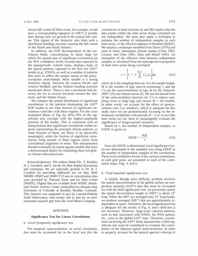
FIG. A1. Distributions of correlations between the global temper-ature anomalies and the ^SIE*& in three climate-sensitive areas withleads 6 months to lags 2 yr (solid line), 1000 white noise series (dot-dashed line), 1000 randomly shuffled ^SIE*& series (dashed line), and1000 colored noise series (dotted line). Note that the white noisedistribution overlaps with the shuffled series distribution.

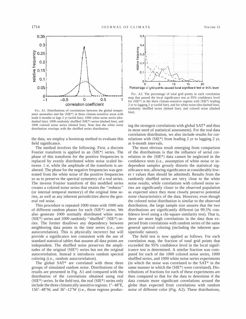
FIG. A2. The percentage of total grid points in each correlationmap that passed the local significance test at 95% confidence levelfor ^SIE*& in the three climate-sensitive regions with ^SIE*& leading2 yr to lagging 2 yr (solid line), and for white noise (dot-dashed line),randomly shuffled series (dotted line), and colored noise (dashedline).

the data, we employ a bootstrap method to evaluate thisfield significance.

The method involves the following. First, a discreteFourier transform is applied to an ^SIE*& series. Thephase of this transform for the positive frequencies isreplaced by evenly distributed white noise scaled be-tween 6p, while the amplitude of the transform is un-altered. The phase for the negative frequencies was gen-erated from the white noise of the positive frequenciesso as to preserve the spectral symmetry of a real series.The inverse Fourier transform of this modified seriescreates a colored noise series that retains the ‘‘redness’’(or internal temporal memory) of the original time se-ries, as well as any inherent periodicities above the gen-eral red noise.

This procedure is repeated 1000 times with 1000 setsof different random phases for each ^SIE*& series. Wealso generate 1000 normally distributed white noise^SIE*& series and 1000 randomly ‘‘shuffled’’ ^SIE*& se-ries. The former disallows any dependency betweenneighboring data points in the time series (i.e., zeroautocorrelation). This is physically incorrect but willprovide a significance test consistent with the use ofstandard statistical tables that assume all data points areindependent. The shuffled noise preserves the ampli-tudes of the original ^SIE*& series but not the originalautocorrelation. Instead it introduces random spectralcoloring (i.e., random autocorrelation).

The global SAT* are correlated with these threegroups of simulated random noise. Distributions of theresults are presented in Fig. A1 and compared with thedistribution of the correlations obtained using real^SIE*& series. In the field test, the real ^SIE*& series onlyinclude the three climatically sensitive regions: 18–488E,1568–488W, and 368–128W (i.e., those regions produc-

ing the strongest correlations with global SAT* and thusin most need of statistical assessment). For the real datacorrelation distribution, we also include results for cor-relations with ^SIE*& from leading 2 yr to lagging 2 yr,at 6-month intervals.

The most obvious result emerging from comparisonof the distributions is that the influence of serial cor-relation in the ^SIE*& data cannot be neglected in theconfidence tests (i.e., assumption of white noise or in-dependent samples grossly distorts the statistical sig-nificance test, allowing significance at considerably low-er r values than should be admitted). Results from therandomly shuffled series are very close to the whitenoise results, while correlations with colored noise se-ries are significantly closer to the observed populationas expected since they most closely preserve potentialnoise characteristics of the data. However, even thoughthe colored noise distribution is similar to the observeddistribution, the large sample size assures that the twodistributions are significantly different (at 99.5% con-fidence level using a chi-square similarity test). That is,there are more high correlations in the data than ex-pected from correlations with random series of the samegeneral spectral coloring (including the inherent qua-siperiodic nature).

The field test is now applied as follows. For eachcorrelation map, the fraction of total grid points thatexceeded the 95% confidence level in the local signif-icance test is determined. A similar fraction was com-puted for each of the 1000 colored noise series, 1000shuffled series, and 1000 white noise series experiments(in which the noise was correlated to the SAT* in thesame manner in which the ^SIE*& were correlated). Dis-tributions of fractions for each of these experiments arethen compared to that for the data to determine if thedata contain more significant correlations around theglobe than expected from correlations with randomnoise of different color (Fig. A2). These distributions,


TABLE A1. Field confidence levels of the four correlation maps inFig. 6 using the colored noise distribution. The results are even moresignificant for those less realistic noise distributions (white and shuf-fled noise).

SIE Ice lagField confidence

level

08–128E728–848W

1208–1328W1208–1328W

0006 months

92%89%78%98%

including those with noise, reflect the influence of thespatial coherence existing in the surface temperaturefield.

As seen in Fig. A2, the distribution of significantcorrelations from the real ^SIE*& series, relative to thatfor the various noise series, is shifted to higher per-centages, reflecting a higher fraction of significant cor-relations. The mode of significant correlations (i.e., thecenter of the primary mode of the distributions in Fig.A2) is 8% for the data and 4% from the colored noiseseries. The means are 8.4% and 5.8%, for the data andcolored noise, respectively. To evaluate the significanceof this difference in mean values, we randomly selected126 numbers (the sample size of the data) from 1000colored noise results used to generate the colored noisedistribution, and then calculated the mean of these 126numbers. This process was repeated 10 000 times. The10 000 means have a Gaussian distribution centered at5.8% with a standard deviation of 0.26% (precisely thevalue predicted by the central limit theorem). The datamean lies over 9 standard deviations from the mean ofthe colored noise. Therefore, the data show significantlymore correlations than expected from correlating to ran-dom noise.

Furthermore, the shift in distributions between thereal and colored noise distributions indicates that thereare more significant correlations in the data than in thecolored noise series in the fraction range more than 6%(i.e., there are more significant correlations coveringmore than 6% of the global grid than expected by ran-dom chance, even accounting for the spectral coloringof the data). A chi-square test of similarity suggests thatthe distributions for the data and colored noise (thatdistribution most representative of the data) are differentat the 99.5% confidence level.

The distribution of the noise can now be used toevaluate the significance of the individual correlationmaps presented in Fig. 6 (the previous test result wasfor the collective total of all maps). The field confidencelevels of the four correlation maps presented in Fig. 6are given in Table A1. For those bands in which thesignificance is lower than 95%, the implication is thatthe spatial correlation pattern is dominated by spatiallycoherent patterns in the SAT* so that geographicallyindependent significant correlations are sparse in thosemaps. Clearly, the different field confidence levels in

these four maps imply that the ^SIE*& at different re-gions respond to different characteristics of the globalsignal.

REFERENCES

Bromwich, D. H., B. Chen, and K. M. Hines, 1998: Global atmo-spheric impacts induced by year-around open water adjacent toAntarctica. J. Geophys. Res., 103 (D10), 11 173–11 189.

Cane, M. A., S. E. Zebiak, and S. C. Dolan, 1986: Experimentalforecasts of El Nino. Nature, 322, 827–832.

Carleton, A. M, 1988: Sea ice–atmosphere signal of the SouthernOscillation in the Weddell Sea, Antarctica. J. Climate, 1, 379–388., 1989: Antarctic sea-ice relationships with indices of the at-mospheric circulation of the Southern Hemisphere. ClimateDyn., 3, 207–220.

Cavalieri, D. J., P. Gloersen, C. L. Parkinson, J. C. Comiso, and H.J. Zwally, 1997: Observed hemispheric asymmetry in global seaice changes. Science, 278, 1104–1106.

Charles, C. D., D. E. Hunter, and R. G. Fairbanks, 1997: Modulatinginfluence of the monsoon and the Southern Oscillation in a 150year long coral record of tropical Indian Ocean surface temper-ature. Science, 277, 925–928.

Chen, W. Y., 1982: Fluctuations in Northern Hemisphere 700-mbheight field associated with the Southern Oscillation. Mon. Wea.Rev., 110, 808–823.

Chiu, L. S., 1983: Antarctic sea ice variations 1973–1980. Variationsin the Global Water Budget, A. Street-Perrott, M. Beran, and R.Ratcliffe, Eds., Reidel, 301–311.

Comiso, J. C., D. J. Cavalieri, C. L. Parkinson, and P. Gloersen, 1997:Passive microwave algorithms for sea ice concentration: A com-parison of two techniques. Remote Sens. Environ., 60 (3), 357–384.

Dai, A., I. Y. Fung, and A. D. Del Genio, 1997: Surface observedglobal land precipitation variations during 1900–1988. J. Cli-mate, 10, 2943–2962.

Davis, R. E., 1976: Predictability of sea surface temperature and sealevel pressure anomalies over the North Pacific Ocean. J. Phys.Oceanog., 6, 249–266.

Fletcher, J. O., 1969: Ice extent in the southern oceans and its relationto world climate. J. Glaciol., 15, 417–427.

Gloersen, P., 1995: Modulation of hemispheric sea-ice cover by ENSOevents. Nature, 373, 503–506., and W. J. Campbell, 1991: Recent variations in Arctic andAntarctic sea-ice covers. Nature, 352, 33–36., , D. J. Cavalieri, J. C. Comiso, C. L. Parkinson, and H.J. Zwally, 1992: Arctic and Antarctic sea ice, 1978–1987: Sat-ellite passive microwave observations and analysis. NASA SP-511, 290 pp.

Godfred-Spenning, C. R., and I. Simmonds, 1996: An analysis ofAntarctic sea ice and extratropical cyclone associations. Int. J.Climatol., 16, 1315–1332.

Grumbine, R. W., 1994: A sea-ice albedo experiment with the NMCMedium Range Forecast model. Wea. Forecasting, 9, 453–456.

Hansen, J. E., and S. Lebedeff, 1987: Global trends of measuredsurface air temperature. J. Geophys. Res., 92, 13 345–13 372., G. Russell, D. Rind, P. Stone, A. Lacis, S. Lebedeff, R. Rudey,and L. Travis, 1983: Efficient three-dimensional global modelsfor climate studies: Models I and II. Mon. Wea. Rev., 111, 609–662.

Hines, K. M., and D. H. Bromwich, 1999: The roles of Arctic andAntarctic sea ice in forcing global climate. Preprints, Fifth Conf.on Polar Meteorology and Oceanography, Dallas, TX, Amer.Meteor. Soc., 39–43.

Horel, J. D., 1984: Complex principal component analysis: Theoryand examples. J. Climate Appl. Meteor., 23, 1660–1673.

Hurrell, J. W., 1995: Decadal trends in the North Atlantic Oscillation:Regional temperature and precipitation. Science, 269, 677–679.


Jacobs, S. S., and J. C. Comiso, 1997: Climate variability in theAmundsen and Bellingshausen Seas. J. Climate, 10, 697–709.

James, I. N., 1988: On the forcing of planetary-scale Rossby wavesby Antarctica. Quart. J. Roy. Meteor. Soc., 114, 619–637.

Johannessen, O. M., M. Miles, and E. Bjorgo, 1995: The Arctic’sshrinking sea ice. Nature, 376, 126–127.

Jones, P. D., 1994: Hemispheric surface air temperature variations:A reanalysis and an update to 1993. J. Climate, 7, 1794–1802.

Julian, P. R., and R. M. Chervin, 1978: A study of the SouthernOscillation and Walker circulation phenomenon. Mon. Wea.Rev., 106, 1433–1451.

Kalnay, E., and Coauthors, 1996: The NCEP/NCAR 40-Year Re-analysis Project. Bull. Amer. Meteor. Soc., 77, 437–471.

Karoly, D. J, 1989: Southern Hemisphere circulation features asso-ciated with El Nino–Southern Oscillation events. J. Climate, 2,1239–1252.

Katz, R. W., and B. G. Brown, 1991: The problem of multiplicity inresearch on teleconnections. Int. J. Climatol., 11, 505–513.

Kawamura, R., 1994: A rotated EOF analysis of global sea surfacetemperature variability with interannual and interdecadal scales.J. Phys. Oceanogr., 24, 707–715.

Krishnamurti, T. N., S.-H. Chu, and W. Iglesias, 1986: On the sealevel pressure of the Southern Oscillation. Arch. Meteor., Geo-phys. Bioklimatol., 34A, 385–425.

Kumar, K. K., 1997: Seasonal forecasting of Indian summer monsoonrainfall: Diagnostics and synthesis of regional and global signals.Ph.D. thesis, Indian Institute of Tropical Meteorology, 301 pp.[Available from Indian Institute of Tropical Meteorology, PashanRd., Pune 411 008, India.]

Large, W. G., and H. van Loon, 1989: Large-scale, low-frequencyvariability of the 1979 FGGE surface buoy drifts and winds overthe Southern Hemisphere. J. Phys. Oceanogr., 19, 216–232.

Ledley, T. S., and Z. Huang, 1997: A possible ENSO signal in theRoss Sea. Geophys. Res. Lett., 24, 3253–3256.

Livezey, R. E., and W. Y. Chen, 1983: Statistical field significanceand its determination by Monte Carlo techniques. Mon. Wea.Rev., 111, 46–59.

Meehl, G. A., 1984: Modeling the earth’s climate. Climatic Change,6, 259–286., 1988: Tropical–midlatitude interactions in the Indian and Pa-cific sectors of the Southern Hemisphere. Mon. Wea. Rev., 116,472–484., 1990: Seasonal cycle forcing of El Nino–Southern Oscillationin a global, coupled ocean–atmosphere GCM. J. Climate, 3, 72–98., 1991: A reexamination of the mechanism of the semiannualoscillation in the Southern Hemisphere. J. Climate, 4, 911–926., and W. M. Washington, 1990: CO2 climate sensitivity andsnow–sea-ice albedo parameterization in an atmospheric GCMcoupled to a mixed layer ocean model. Climatic Change, 16,283–306.

Mitchell, J. F. B., and T. S. Hills, 1986: Sea-ice and the Antarcticwinter circulation: A numerical experiment. Quart. J. Roy. Me-teor. Soc., 112, 953–969.

Mo, K. C., and G. H. White, 1985: Teleconnections in the SouthernHemisphere. Mon. Wea. Rev., 113, 22–37.

National Snow and Ice Data Center, 1997: Passive microwave deriveddaily polar sea ice concentration time series. Digital data. [Avail-able from NSIDC Distributed Active Archive Center, Universityof Colorado at Boulder, Boulder, CO 80309; also available [email protected].]

Orlanski, I., J. Katzfey, C. Menendez, and M. Marino, 1991: Sim-ulation of an extratropical cyclone in the Southern Hemisphere:Model sensitivity. J. Atmos. Sci., 48, 2293–2311.

Parish, T. R., 1984: A numerical study of strong katabatic winds overAntarctica. Mon. Wea. Rev., 112, 545–554., 1992: On the role of Antarctic katabatic winds in forcing large-scale tropospheric motions. J. Atmos. Sci., 49, 1374–1385.

Parker, D. E., P. D. Jones, A. Bevan, and C. K. Folland, 1994: In-

terdecadal changes of surface temperature since the late 19thcentury. J. Geophys. Res., 99, 14 373–14 399., C. K. Folland, and M. Jackson, 1995: Marine surface temper-ature: Observed variations and data requirements. ClimaticChange, 31, 559–600.

Parkinson, C. L., 1992: Interannual variability of monthly southernocean sea ice distributions. J. Geophys. Res, 97, 5349–5363., 1994: Spatial patterns in the length of the sea ice season in theSouthern Ocean, 1979–1986. J. Geophys. Res., 99, 16 327–16 339.

Peng, G. B., and P. K. Wang, 1989: Influence of the Antarctic sea-ice on the Northwest Pacific sub-tropical high and its backgroundof ocean–atmospheric circulation. Chin. Sci. Bull., 34, 1463–1465.

Peterson, R. G., and W. B. White, 1998: Slow teleconnections linkingthe Antarctic Circumpolar Wave with the tropical El Nino–Southern Oscillation. J. Geophys. Res., 103 (C11), 24 573–24 583.

Rasmusson, E. M., and T. H. Carpenter, 1982: Variations in tropicalsea surface temperature and wind fields associated with theSouthern Oscillation/El Nino. Mon. Wea. Rev., 110, 354–384.

Reuter, E., 1936: Die synoptische Darstellung der 1/2 jahrigen Druck-welle. Veroff. Geophys. Inst. Univ. Leipzig, 7, 257–295.

Reynolds, R. W., and T. M. Smith, 1994: Global sea surface tem-perature analysis. J. Climate, 7, 929–948.

Rind, D., R. Healy, C. Parkinson, and D. Martinson, 1995: The roleof sea ice in 2XCO2 climate model sensitivity. Part I: The totalinfluence of sea ice thickness and extent. J. Climate, 8, 449–463.

Roberts, J., and T. D. Roberts, 1978: Use of the Butterworth low-pass filter for oceanographic data. J. Geophys. Res., 83, 5510–5514.

Schwerdtfeger, W., 1960: The seasonal variation of the strength ofthe southern circumpolar vortex. Mon. Wea. Rev., 88, 203–208., 1962: The southern circumpolar vortex and the spring warmingof the polar stratosphere. Meteor. Abh., 36, 207–224., and St. J. Kachelhoffer, 1973: The frequency of cyclone vorticesover the southern ocean in relation to the extension of the packice belt. Antarct. J., 8, 234.

Simmonds, I., and M. Dix, 1986: The circulation changes inducedby the removal of Antarctic sea ice in a July general circulationmodel. Extended Abstracts, Second Int. Conf. on Southern Hemi-sphere Meteorology, Wellington, New Zealand, Amer. Meteor.Soc., 107–110., and X. Wu, 1993: Cyclone behaviour response to changes inwinter Southern Hemisphere sea-ice concentration. Quart. J.Roy. Meteor. Soc., 119, 1121–1148., and T. H. Jacka, 1995: Relationships between the interannualvariability of Antarctic sea ice and the Southern Oscillation. J.Climate, 8, 637–647., and R. Law, 1995: Associations between antarctic katabaticflow and the upper level winter vortex. Int. J. Climatol., 15, 403–421., and D. A. Jones, 1998: The mean structure and temporal var-iability of the semiannual oscillation in the southern extratropics.Int. J. Climatol., 18, 473–504.

Smith, R. C., S. E. Stammerjohn, and K. S. Baker, 1996: Surface airtemperature variations in the western Antarctic Peninsula region.Foundations for Ecological Research West of the Arctic Pen-insula, R. M. Ross, E. E. Hofmann, and L. B. Quetin, Eds.,Antarctic Research Series, Vol. 70, Amer. Geophys. Union, 105–121.

Smith, S. R., and C. R. Stearns, 1993: Antarctic pressure and tem-perature anomalies surrounding the minimum in the SouthernOscillation index. J. Geophys. Res., 98 13 071–13 083.

Stammerjohn, S. E., and R. C. Smith, 1996: Spatial and temporalvariability of the western Antarctic Peninsula sea ice coverage.Foundations for Ecological Research West of the Antarctic Pen-insula, R. M. Ross, E. E. Hofmann, and L. B. Quetin, Eds.,


Antarctic Research Series, Vol. 70, Amer. Geophys. Union, 81–104., and , 1997: Opposing Southern Ocean climate patterns asrevealed by trends in regional sea ice coverage. Climatic Change,37, 617–639.

Streten, N. A., and D. J. Pike, 1980: Characteristics of the broadscaleAntarctic sea ice extent and the associated atmospheric circu-lation 1972–1977. Arch. Meteor., Geophys. Bioklimatol., 29A,279–299.

Taljaard, J. J., 1972: Physical features of the Southern Hemisphere.Meteorology of the Southern Hemisphere, Meteor. Monogr., No.35, Amer. Meteor. Soc., 1–8.

Thompson, D. W. J., and J. M. Wallace, 1998: The Arctic Oscillationsignature in the wintertime geopotential height and temperaturefields. Geophys. Res. Lett., 25, 1297–1300.

Tourre, M. Y., and W. B. White, 1995: ENSO signals in global upper-ocean temperature. J. Phys. Oceanogr., 25, 1317–1332.

Trenberth, K. E., 1980: Planetary waves at 500 mb in the SouthernHemisphere. Mon. Wea. Rev., 108, 1378–1389., W. G. Large, and J. G. Olson, 1990: The mean annual cyclein global ocean wind stress. J. Phys. Oceanogr., 20, 1742–1760.

van Loon, H., 1967: The half-yearly oscillations in middle and highsouthern latitudes and the coreless winter. J. Atmos. Sci., 24,472–486., 1972: Wind in the Southern Hemisphere. Meteorology of theSouthern Hemisphere, Meteor. Monogr., No. 35, Amer. Meteor.Soc., 87–100., 1984: The Southern Oscillation. Part III: Associations with thetrades and with the trough in the westerlies of the South PacificOcean. Mon. Wea. Rev., 112, 947–954.

, and R. L. Jenne, 1972: The zonal harmonic standing waves inthe Southern Hemisphere. J. Geophys. Res., 77, 992–1003., , and K. Labitzke, 1973: Zonal harmonic standing waves.J. Geophys. Res., 78, 4463–4471.

Walker, G. T., 1923: Correlation in seasonal variations of weather,VIII. Mem. Indian Meteor. Dept., 24, 75–131., 1924: Correlation in seasonal variations of weather, IX. Mem.Indian Meteor. Dept., 24, 275–322.

Wallace, J. M., and R. E. Dickinson, 1972: Empirical orthogonalrepresentation of time series in the frequency domain. Part I:Theoretical considerations. J. Appl. Meteor., 11, 887–900.

Walsh, J. E., 1983: The role of sea ice in climatic variability: Theoriesand evidence. Atmos.–Ocean, 21 (3), 229–242.

Weatherly, J. W., J. E. Walsh, and H. J. Zwally, 1991: Antarctic seaice variations and seasonal air temperature relationships. J. Geo-phys. Res., 96, 15 119–15 130.

White, W. B., and R. G. Peterson, 1996: An Antarctic circumpolarwave in surface pressure, wind, temperature and sea ice extent.Nature, 380, 699–702., S.-C. Chen, and R. G. Peterson, 1998: The Antarctic circum-polar wave: A beta effect in ocean–atmosphere coupling overthe Southern Ocean. J. Phys. Oceanogr., 28, 2345–2361.

Yuan, X., M. A. Cane, and D. G. Martinson, 1996: Climate varia-tion—Cycling around the South Pole. Nature, 380, 673–674.

Zhao, W., and M. A. K. Khalil, 1993: The relationship between pre-cipitation and temperature over the contiguous United States. J.Climate, 6, 1232–1236.

Zwally, H. J., J. C. Comiso, C. L. Parkinson, W. J. Campbell, F. D.Carsey, and P. Gloerson, 1983: Antarctic sea ice, 1973–1976:Satellite passive-microwave observations. NASA SP-459, 200pp.

Antarctic Sea Ice Extent Variability and Its Global ...

Documents

Transcript of Antarctic Sea Ice Extent Variability and Its Global ...