A n t C o l o n i e s f o r t h e

Q u a d r a t i c A s s i g n m e n t P r o b l e m

L. M. GAMBARDELLA, É. D. TAILLARDIDSIA, Corso Elvezia 36, CH-6900 Lugano, Switzerland

luca@idsia.ch, eric@idsia.ch, http://www.idsia.chtel: +41-91-9119838, fax: +41-91-9119839

M. DORIGOIRIDIA - CP 194/6, Université Libre de Bruxelles

Avenue Franklin Roosevelt 50, 1050 Bruxelles, Belgiummdorigo@ulb.ac.be, http://iridia.ulb.ac.be/dorigo/dorigo.html

tel: +32-2-6503169, fax: +32-2-6502715

This paper presents HAS-QAP, a hybrid ant colony system coupled with a local search, applied to thequadratic assignment problem. HAS-QAP uses pheromone trail information to perform modifications onQAP solutions, unlike more traditional ant systems that use pheromone trail information to constructcomplete solutions. HAS-QAP is analysed and compared with some of the best heuristics available for theQAP: two versions of tabu search, namely, robust and reactive tabu search, hybrid genetic algorithm, and asimulated annealing method. Experimental results show that HAS-QAP and the hybrid genetic algorithmperform best on real world, irregular and structured problems due to their ability to find the structure of goodsolutions, while HAS-QAP performance is less competitive on random, regular and unstructured problems.

Key words: Quadratic assignment problem, ant colony optimisation, ant systems, meta-heuristics.

INTRODUCTION

The quadratic assignment problem

The QAP is a combinatorial optimisation problem stated for the first time by Koopmans andBeckman1 in 1957. It can be described as follows: Given two n × n matrices A=(aij) and B=(bij),

find a permutation π * minimising

∑∑= =

Π∈⋅=

n

i

n

jijn ji

baf1 1

)()(min πππ

π

where Π(n) is the set of permutations of n elements. Shani and Gonzalez2 have shown that theproblem is NP-hard and that there is no ε-approximation algorithm for the QAP unless P = NP.While some NP-hard combinatorial optimisation problems can be solved exactly for relatively largeinstances, as exemplified by the travelling salesman problem (TSP), QAP instances of size largerthan 20 are considered intractable. In practice, a large number of real world problems lead to QAPinstances of considerable size that cannot be solved exactly. For example, an application in imageprocessing requires solving more than 100 problems of size n = 256 (Taillard3). The use of heuristicmethods for solving large QAP instances is currently the only practicable solution.

Heuristic methods for the QAPA large number of heuristic methods have been developed for solving the QAP, using various

techniques. Very briefly, the most notable methods are the following: the simulated annealing ofConnolly4, the tabu searches of Taillard5, Battiti and Tecchiolli6 and Sondergeld and Voß7, and thehybrid genetic-tabu search of Fleurent and Ferland8. More recently, another promising method hasbeen developed based on scatter search by Cung, Mautor, Michelon and Tavares9. This newmethod embeds a tabu search.

This paper presents a hybrid ant-local search system for the QAP that often works better thanthe above mentioned heuristics on structured problems. The paper is organised as follows: In thenext section ant systems in general are described. Our hybrid ant-local search system is presented inthe following section. Then, the performance of our algorithm is analysed by comparing it to the bestexisting methods, and in the last section some conclusions are drawn.

ANT SYSTEMThe idea of imitating the behaviour of ants for finding good solutions to combinatorial optimisation

problems was initiated by Dorigo, Maniezzo and Colorni10,11, and Dorigo12. The principle of thesemethods is based on the way ants search for food and find their way back to the nest13. Initially, antsexplore the area surrounding their nest in a random manner. As soon as an ant finds a source of food

it evaluates quantity and quality of the food and carries some of this food to the nest. During thereturn trip, the ant leaves a chemical pheromone trail on the ground. The role of this pheromone trailis to guide other ants toward the source of food, and the quantity of pheromone left by an antdepends on the amount of food found. After a while, the path to the food source will be indicated bya strong pheromone trail and the more the ants which reach the source of food, the stronger thepheromone trail left.

Since sources that are close to the nest are visited more frequently than those that are far away,pheromone trails leading to the nearest sources grow more rapidly. These pheromone trails areexploited by ants as a means to find their way from nest to food source and back.The transposition of real ants food searching behaviour into an algorithmic framework for solvingcombinatorial optimisation problems is done by making an analogy between 1) the real ants’ searcharea and the set of feasible solutions to the combinatorial problem, 2) the amount of food in a sourceand the objective function, and 3) the pheromone trail and an adaptive memory. A detaileddescription of how these analogies can be put to work in the TSP case can be found in Dorigo,Maniezzo and Colorni10,11. An up-to-date list of papers and applications of ant colony optimisationalgorithms is maintained on the WWW at the address: http://iridia.ulb.ac.be/dorigo/ACO/ACO.html.

The present paper shows how these analogies can be put to work in the case of the quadraticassignment problem (QAP). The resulting method, Hybrid Ant System for the QAP, HAS-QAP forshort, is shown to be efficient for solving structured QAP’s.

HYBRID ANT SYSTEM FOR THE QAPThis section presents the HAS-QAP algorithm and compares and analyses its main components

in relation to previous ant inspired systems. Very shortly, Hybrid Ant System for the QAP is basedon the schematic algorithm of Figure 1.

Pheromone trailThe most important component of an ant system is the management of pheromone trails. In a

standard ant system, pheromone trails are used in conjunction with the objective function forconstructing a new solution. Informally, pheromone levels give a measure of how desirable it is toinsert a given element into a solution. For example, in Dorigo and Gambardella’s14 TSP application,links get a higher amount of pheromone if they are used by ants which make shorter tours.Pheromone trails in this case are maintained in a pheromone matrix T = (τij) where τij measures how

desirable the edge between cities i and j is. For the QAP, the set of the pheromone trails ismaintained in a matrix T = (τij) of size n × n, where the entry τij measures the desirability of settingπ i = j in a solution.

There are two different uses of pheromone: exploration and exploitation. Exploration is astochastic process in which the choice of the component used to construct a solution to the problemis made in a probabilistic way. Exploitation chooses the component that maximises a blend ofpheromone trail values and partial objective function evaluations.

After having built a new solution, a standard ant system updates the pheromone trails as follows:first, all the pheromone trails are decreased to simulate the evaporation of pheromone. Then, thepheromone trails corresponding to components that were chosen for constructing the solution arereinforced, taking into consideration the quality of the solution.

Since the first implementation of an ant system (Dorigo, Maniezzo and Colorni10), it has beenchanged in many ways to improve its efficiency. In the best ant system to date (Dorigo andGambardella14) update of pheromone trails is very loosely coupled with what happens with real ants.Indeed, pheromone trails are not only modified directly and locally by the artificial agents during orjust after the construction of a new solution, but also globally, considering the best solutiongenerated by all the agents at a given iteration or even the best solution ever constructed. In HAS-QAP, local updates of the pheromone trails are not performed, but only a global update. This makesthe search more aggressive and requires less time to reach good solutions. Moreover, this has beenstrengthened by an intensification mechanism. An inconvenience of such a process is the risk of anearly convergence of the algorithm. Therefore, a diversification mechanism that periodically erasesall the pheromone trails has been added.

Solutions manipulationAnother peculiarity of HAS-QAP is the use of the pheromone trails in a non-standard way: in

preceding applications of ant systems (Dorigo, Maniezzo and Colorni10,11, Dorigo andGambardella14), pheromone trails were exploited to build a completely new solution. Here,pheromone trails are used to modify an existing solution, in the spirit of a neighbourhood search.After an artificial agent has modified a solution, taking into account only the information contained inthe pheromone trail matrix, an improvement phase that consists in performing a fast local search thattakes into consideration only the objective function is applied.

Adding local search to ant systems has also been identified as very promising by otherresearchers: for the TSP, Dorigo and Gambardella14 succeeded in designing an ant system almost asefficient as the best implementations of the Lin and Kernighan heuristic by adding a simple 3-optphase after the construction phase; for the sequential ordering problem (SOP) Gambardella andDorigo15 alternate an ant system with a local search specifically designed for the SOP, obtaining verygood results and new upper bounds for a large set of test problems.

In fact, many of the most efficient heuristic methods for combinatorial optimisation problems arebased on a neighbourhood search, either a greedy local search or a more elaborate meta-heuristiclike tabu search (e.g., see Battiti and Tecchiolli6, Cung et al.9, Fleurent and Ferland8, Taillard5,Sondergeld and Voß7 for applications to the QAP) or simulated annealing (see e. g. Burkard andRendl16, and Connolly4).

Intensification and diversificationAs said, in HAS-QAP each ant is associated with a problem solution that is first modified using

pheromone trail and later is improved using a local search mechanism. This approach is completely

different from that of previous ant systems where solutions were not explicitly associated with antsbut were created in each iteration using a constructive mechanism.

Therefore, in HAS-QAP, there is the problem of choosing, during each iteration, the startingsolution associated to each ant. To solve this problem two mechanisms, called intensification anddiversification, have been defined. Intensification is used to explore the neighbourhood of goodsolutions more completely. When intensification is active, the ant comes back to the solution it had atthe beginning of the iteration if this solution was better than the solution it had at the end of theiteration; in all other cases, the ant simply continues working on its current solution. Diversificationimplements a partial restart of the algorithm when the solutions seem not to be improving any more.It consists in a re-initialisation of both the pheromone trail matrix and the solutions associated to theants.

HAS-QAP DESCRIPTIONThis section discusses the most salient aspects of HAS-QAP algorithm, which is presented into

details in Figure 2.

Initialisation of solutionsInitially, each ant is given a randomly chosen permutation. These permutations are initially

optimised using the same local search procedure that will be described later.

Pheromone trail initialisationInitially no information is contained in the pheromone trail matrix: all pheromone trails τij are set to

the same value τ0. Since pheromone trails are updated by taking into account the absolute value ofthe solution obtained, τ0 must take a value that depends on the value of the solutions that will bevisited. Therefore, we have chosen to set τ0 = 1/(Q·f(π *)), where π * is the best solution found so

far and Q a parameter. The re-initialisations of the pheromone trails are done in the same way, butπ * might have changed.

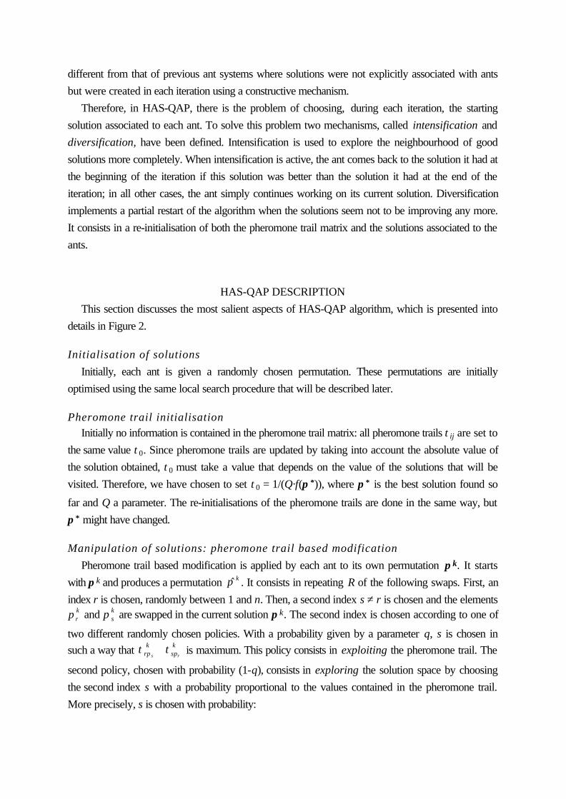
Manipulation of solutions: pheromone trail based modificationPheromone trail based modification is applied by each ant to its own permutation π k. It starts

with π k and produces a permutation $π k . It consists in repeating R of the following swaps. First, anindex r is chosen, randomly between 1 and n. Then, a second index s ≠ r is chosen and the elementsπ r

k and π sk are swapped in the current solution π k. The second index is chosen according to one of

two different randomly chosen policies. With a probability given by a parameter q, s is chosen insuch a way that τ τπ πr

ksk

s r+ is maximum. This policy consists in exploiting the pheromone trail. The

second policy, chosen with probability (1-q), consists in exploring the solution space by choosingthe second index s with a probability proportional to the values contained in the pheromone trail.More precisely, s is chosen with probability:

τ τ

τ τπ π

π π

rk

sk

rk

jk

j r

s r

j r

+

+≠∑ ( )

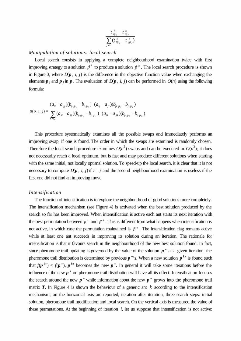
Manipulation of solutions: local searchLocal search consists in applying a complete neighbourhood examination twice with first

improving strategy to a solution $π k to produce a solution ~π k . The local search procedure is shownin Figure 3, where ∆(π , i, j) is the difference in the objective function value when exchanging theelements π i and π j in π . The evaluation of ∆(π , i, j) can be performed in O(n) using the following

formula:

∆( , , )π i j = ∑≠

−−+−−

+−−+−−

jikjkikkjki

jiijjjii

kikjikjk

jiijiijj

bbaabbaa

bbaabbaa

,

))(())((

))(())((

ππππππππ

ππππππππ

This procedure systematically examines all the possible swaps and immediately performs animproving swap, if one is found. The order in which the swaps are examined is randomly chosen.Therefore the local search procedure examines O(n2) swaps and can be executed in O(n3); it doesnot necessarily reach a local optimum, but is fast and may produce different solutions when startingwith the same initial, not locally optimal solution. To speed-up the local search, it is clear that it is notnecessary to compute ∆(π , i, j) if i = j and the second neighbourhood examination is useless if thefirst one did not find an improving move.

IntensificationThe function of intensification is to explore the neighbourhood of good solutions more completely.

The intensification mechanism (see Figure 4) is activated when the best solution produced by thesearch so far has been improved. When intensification is active each ant starts its next iteration withthe best permutation between kπ and ~π k . This is different from what happens when intensification isnot active, in which case the permutation maintained is ~π k . The intensification flag remains activewhile at least one ant succeeds in improving its solution during an iteration. The rationale forintensification is that it favours search in the neighbourhood of the new best solution found. In fact,since pheromone trail updating is governed by the value of the solution π * at a given iteration, thepheromone trail distribution is determined by previous π *’s. When a new solution π k* is found suchthat f(π k*) < f(π *), π k* becomes the new π *. In general it will take some iterations before theinfluence of the new π * on pheromone trail distribution will have all its effect. Intensification focusesthe search around the new π * while information about the new π * grows into the pheromone trailmatrix T. In Figure 4 is shown the behaviour of a generic ant k according to the intensificationmechanism; on the horizontal axis are reported, iteration after iteration, three search steps: initialsolution, pheromone trail modification and local search. On the vertical axis is measured the value ofthese permutations. At the beginning of iteration i, let us suppose that intensification is not active:

therefore, kπ (i + 1) ← ( )~π k i . At the end of iteration i + 1, kπ (i + 2) is set again to ( )1~ +ikπ and

intensification is activated because the best known solution has improved. At the end of iterationi + 2, kπ (i + 3) is set to kπ (i + 2) because intensification is active and kπ (i + 2) is a better solutionthan ( )~π k i + 2 .

Pheromone trail updateThe update of the pheromone trails is done differently from the standard ant system where all the

ants update the pheromone trails with the result of their computations. Indeed, this manner ofupdating the pheromone trails determines a very slow convergence of the algorithm (Dorigo andGambardella14). To speed-up the convergence, the pheromone trails are updated by taking intoaccount only the best solution produced by the search to date. First, all the pheromone trails areweakened by setting τij = (1 – α 1)·τij, (1 ≤ i, j ≤ n) where 0 < α 1< 1 is a parameter that controls

the evaporation of the pheromone trail: a value of α 1 close to 0 implies that the pheromone trailsremain active a long time, while a value close to 1 implies a high degree of evaporation and a shortermemory of the system. Then, the pheromone trails are reinforced by considering only π *, that is, thebest solution generated by the system so far and setting τiπi* = τiπi* + α 2/f(π *) for all i.

DiversificationThe aim of diversification is to constrain the algorithm to work on solutions with different

structure. The diversification mechanism is activated if during the last S iterations no improvement tothe best generated solution is detected. Diversification consists in erasing all the informationcontained in the pheromone trails by a re-initialisation of the pheromone trail matrix and in generatingrandomly a new current solution for all the ants but for one ant that preserves the best solutionproduced by the search so far.

Complexity and memory requirementThe complexity of the HAS-QAP algorithm can be evaluated as follows: the most time

consuming part of the algorithm is the local search procedure. The complexity of this step is O(n3)and it is repeated Imaxm times. Therefore the total complexity of HAS-QAP is O(Imaxmn3). Thememory size required by the algorithm is O(n2 + nm) since the data matrices have to be stored aswell as m permutations.

NUMERICAL RESULTSHAS-QAP is compared with a number of the best heuristic methods available for the QAP such

as the genetic hybrid method of Fleurent and Ferland8 (GH), the reactive tabu search of Battiti andTecchiolli6 (RTS), the tabu search of Taillard5 (TT) and a simulated annealing due to Connolly4

(SA). For the comparison, a large subset of well known problem instances is considered, with sizesbetween n = 19 and n = 90, and contained in the QAPLIB compiled by Burkard, Karisch andRendl

17.

As shown by Taillard3, the quality of solutions produced by heuristic methods strongly depends

on the problem type, that is, on the structure of the data matrices A and B. Generally, instances ofproblems taken from the real world present at least one matrix with very variable entries, forexample with a majority of zeros. For such problems, many heuristic methods perform rather poorly,being unable to find solutions below 10% of the best solutions known, even if an excessivecomputing time is allowed. Moreover, this occurs also for problems of small size. Conversely, thesame methods may perform very well on randomly generated problems with matrices that haveuniformly distributed entries. For such problems, almost all heuristic methods are able to find highquality solutions (i.e., solutions approximately one per cent worse than the best solution known).

For real world problems, Taillard3 found that GH was one of the best performing, in particular interms of the quality of the solutions obtained. For problems with matrices that have uniformlydistributed entries RTS and TT perform best. Therefore the performance of HAS-QAP has beenanalysed by splitting the problem instances into two categories: (i) real world, irregular andstructured problems, and (ii) randomly generated, regular and unstructured problems. The problemshave been classified using a simple statistic known as "flow-dominance"18,19. Let µA (respectively µB)be the average value of the off-diagonal elements of matrix A (respectively B), and σA (respectivelyσB) the corresponding standard deviation. A problem is put in category (i) if max(σA /µA, σB /µB) >1.2 and in category (ii) otherwise. In tables 1 and 3 is reported the flow dominance value for thetested problems.

All the algorithms used for comparisons were run with the parameter settings proposed by theirauthors, except for GH, where a population of min(100, 2n) solutions was used instead of 100solutions in order to improve the method (see also Taillard3). It is important to note that RTS is amethod with self-adapting parameters (i.e., the only parameter set by the user is the number ofiterations) and the SA cooling scheme is also self-adapted, with the total number of iterations set bythe user.

The complexity of one iteration for each algorithm considered varies: SA has the lowercomplexity with O(n) per iteration. TT and RTS have a complexity of O(n2) per iteration while GHand HAS have a complexity of O(n3).

The time needed to execute one HAS-QAP iteration on a size n problem was experimentally setto a value that corresponds, using the software implementations tested, to approximately the timeneeded to perform 10n iterations of RTS and TT, 125n2 iterations of SA and 2.5 iterations of GH.

In order to make fair comparisons between these algorithms, the same computational time wasgiven to each test problem trial by performing a number of iterations equal to Imax for HAS-QAP, to10nImax for RTS and TT, 125n2Imax for SA and 2.5Imax for GH.

In addition, results for two values of Imaxare provided: short runs with Imax=10 and long runs withImax=100. The reason to compare algorithms on short and on long runs is to evaluate their ability inproducing relatively good solutions under strong time constraints versus producing very goodsolutions where more computational resources are available. In addition, short runs are interesting

when these methods are used to produce starting solutions for different algorithms or to deal withproblems of large size.

HAS-QAP parameters settingFor HAS-QAP the following parameter settings were used: R = n/3, α 1 = α 2= 0.1, Q = 100,

S = n/2, q = 0.9 and m = 10. These parameters were experimentally found to be good and robustfor the problems tested.

For parameter R, the number of swaps executed using pheromone trail information, R = n/3 hasbeen shown experimentally to be more efficient than n/2 and n/6. Starting from π k a newpermutation $π k is generated by performing R pheromone trail driven exchanges, then $π k isoptimised to produce permutation ~π k using the local search procedure. In case of R ≥ n/2 theresulting permutation $π k tends to be too close to the solution π * used to perform global pheromonetrail updating, which makes it more difficult to generate new improving solutions. On the contrary,R ≤ n/6 did not allow the system to escape from local minima because, after the local search,~π k was in most cases the same as the starting permutation π k.

Same type of experiments and considerations have been made to define other parameters, likeα 1=α 2 and Q=100. In addition, the importance of diversification (parameter S) and exploration(parameter q) was tested by running different experiments in which the parameters S and q were setto S = ∞ (no diversification) and/or q = 1 (no exploration). In all these cases, the algorithmperformance was worse in comparison with the performance obtained using the proposed values(S = n/2 and q = 0.9). For S close to n and S ≤ n/6 phenomena of stagnation and insufficientintensification have been observed. The choice of setting the number of ants to m=10 is discussed inthe following sections.

In general, experiments have shown that the proposed parameter setting is very robust to smallmodifications.

Real world, irregular and structured problemsFrom the QAPLIB, 20 problems were selected which have values of the flow-dominance

statistic larger than 1.2. Most of these problems come from practical applications or have beenrandomly generated with non uniform laws, imitating the distributions observed on real worldproblems. As mentioned above, comparisons were run with the tabu searches of Battiti andTecchiolli6 (RTS) and Taillard5 (TT), and the genetic-hybrid method of Fleurent and Ferland8 (GH).A simulated annealing due to Connolly4 (SA) that is cited as a good implementation by Burkard andÇela20 was also considered. GH, TT and SA methods have been re-programmed, while the originalcode has been used for RTS. Unfortunately, this code only considers symmetric problems.Therefore, problems with an asymmetric matrix have not been solved with RTS.

Table 1 compares all these methods on short executions: Imax = 10 for HAS-QAP. In particular,the average quality of the solutions produced by these methods is shown, measured in per centabove the best solution value known; the last column of this table reports the computing time(seconds on a Sun Sparc 5) used for each test problem trial. All the methods were run 10 times. The

best results are in italic boldface. To assess the statistical significance of the differences among meansthe Mann-Whitney U-test (Siegel and Castellan21) has been run (this is the non-parametriccounterpart of the t-test for independent samples; the t-test cannot be used here because of thelimited dimensions of the samples and for the nature of data). For each problem, that is for each rowof the table, the Mann-Whitney U-test was run between the best result (italic boldface) and each ofthe results obtained with the other meta-heuristics. Whenever the two results are not significantlydifferent at the 0.1 level, this is indicated in the table by boldface characters (e.g., in Table 1 forproblem bur26b, GH resulted to be the best meta-heuristic; SA and HAS-QAP were found to benot statistically different at the 0.1 level; it can therefore be said that for this problem SA, GH, andHAS-QAP were the best meta-heuristics). The same procedure was applied in the following tables.

From Table 1, it is clear that methods like TT or SA are not well adapted for irregular problems.Sometimes, they produce solutions more than 10% worse than the best solutions known while otherheuristic methods are able to exhibit solutions at less than 1% with the same computing effort. Forthe problem types bur... and tai..b, HAS-QAP seems to be the best method overall. The only realcompetitor of HAS-QAP for irregular problems is GH. (Or, more precisely, the repetition of 25independent tabu searches with 4n iterations: Indeed, the genetic algorithm of Fleurent and Ferland8

is hybridised with TT; each solution produced by this method is improved with 4n iterations of TTbefore being eventually inserted in the population. After 25 iterations, the GH algorithm is still in theinitialisation phase that consists in building initial solutions issued from min(100, 2n) repetitions of TTstarting with random initial solutions), while SA is never really competitive.

In Table 2 are shown results obtained with HAS-QAP on longer runs, setting Imax = 100. Whenall the 10 runs of HAS-QAP succeeded in finding the best solution known, it is added in parenthesesthe average computing time (seconds) for reaching the best solution known; the time for completing100 iterations is roughly 10 times that for 10 iterations. From this table, the same conclusions as forshorter runs can be drawn. As above, Mann-Whitney U-tests was run and found that for allinstances but two HAS-QAP was one of the best methods.

Randomly generated, regular and unstructured problemsFor unstructured problems, the solutions produced by HAS-QAP are not as good as for

structured problems. This can be explained by the fact that relatively good solutions of theseproblems are spread in the whole feasible solution set (see the entropy measure of local optimareported in Taillard3).

The main strength of HAS-QAP, as well as of the GH algorithm, is its ability in finding thestructure of good solutions. If all the good solutions are concentrated in a close subset of the feasiblesolutions, GH and HAS-QAP work well. On the contrary, these algorithms are not performing wellwhen a large number of relatively good solutions are spread all over the solutions space. Tables 3and 4, provide the same results as those of tables 1 and 2, but for unstructured problems.

These tables show that TT, GH and SA perform best for sko.. problems and RTS performs bestfor tai..a problems, while HAS-QAP is not so good and even the worst method for tai..aproblems.

Number of AntsThe application of the ant colony approach to a combinatorial problem like the QAP makes

sense only if it gives some performance advantage. It is interesting therefore to experimentallyevaluate the performance gain obtained, given a same amount of computation time, by using agrowing number of ants. To this purpose, for each of the four experimental situations studied (shortand long runs, structured and unstructured problems), the average performance of HAS-SOP wasanalysed, when varying the number of ants. The average performance of HAS-SOP was defined asthe average over the problems reported in each of the tables 1 to 4. To limit the computation timerequired to evaluate these averages, experiments were run only on problems with n<60. The numberof ants was set to m = {1, 5, 10, 20}. The results, reported in Table 5, show that the choice m=10is always optimal but for the case of short runs and unstructured problems.

CONCLUSIONSRecent results in the application of heuristic methods to the solution of difficult combinatorial

problems seem to indicate that combining local optimisation with good heuristic ways of generatingstarting solutions for the local searches can give rise to powerful, although approximate, optimisationalgorithms. Ant colony optimisation is a recent heuristic loosely based on the observation of someaspects of ant colonies behaviour (Dorigo, Maniezzo and Colorni10,11, Dorigo12). In this paperresults on the quadratic assignment problem obtained by HAS-QAP, an algorithm which interleavesan ant colony algorithm with a simple local search have been presented. Comparisons with some ofthe best heuristics for the QAP have shown that our approach is among the best as far as real world,irregular, and structured problems are concerned. The only competitor was shown to be Fleurentand Ferland’s8 genetic-hybrid algorithm. On the other hand, on random, regular, and unstructuredproblems the performance of HAS-QAP was less competitive and tabu searches are still the bestmethods. So far, the most interesting applications of ant colony optimisation were limited tosymmetric, asymmetric and constrained travelling salesman problems (Dorigo and Gambardella14,Gambardella and Dorigo15). With this paper the spectrum of successful applications of ant colonyalgorithms has been widened to include structured quadratic assignment problems.

Acknowledgements — Marco Dorigo is a Research Associate with the Belgian FNRS. This research has been funded by theSwiss National Science Foundation contract 21–45653.95 titled “Co-operation and learning for combinatorial optimisation.”

REFERENCES1 Koopmans T C and Beckmann M J (1957). Assignment problems and the location of economics activities.

Econometrica 25: 53–76.

2 Shani S and Gonzalez T (1976). P-complete approximation problems. Journal of the ACM 23: 555–565.

3 Taillard É D (1995). Comparison of iterative searches for the quadratic assignment problem. Location Science 3: 87–105.

4 Connolly D T (1990). An improved annealing scheme for the QAP. Eur J Op Res 46: 93–100.

5 Taillard É D (1991). Robust taboo search for the quadratic assignment problem. Parallel Computing 17: 443–455.

6 Battiti R and Tecchiolli G (1994). The reactive tabu search. ORSA J on Computing 6: 126-140.

7 Sondergeld L and Voß S (1996). A star-shaped diversification approach in tabu search. In: Osman I H and KellyJ P (eds). Meta-Heuristics: Theory and Applications. Kluwer Academic Publishers: Boston/London/Dordnecht, pp 489–502.

8 Fleurent C and Ferland J (1994). Genetic hybrids for the quadratic assignment problem. DIMACS Series in Mathematicsand Theoretical Computer Science 16: 190–206.

9 Cung V-D, Mautor T, Michelon P and Tavares A (1997). A scatter search based approach for the quadratic assignmentproblem. Proceedings of the IEEE International Conference on Evolutionary Computation and EvolutionaryProgramming. (ICEC’ 97), Indianapolis, USA, pp 165-170.

10 Dorigo M, Maniezzo V and Colorni A (1991). Positive feedback as a search strategy. Technical Report 91-016,Dipartimento di Elettronica e Informazione, Politecnico di Milano, Italy.

11 Dorigo M, Maniezzo V and Colorni A (1996). The ant system: Optimization by a colony of cooperating agents. IEEETransactions on Systems, Man, and Cybernetics–Part B 26: 29–41.

12 Dorigo M (1991). Ottimizzazione, apprendimento automatico, ed algoritmi basati su metafora naturale (Optimisation,learning and natural algorithms). Doctoral dissertation, Dipartimento di Elettronica e Informazione, Politecnico diMilano, Italy.

13 Goss S, Aron, Deneubourg JL and Pasteels J M (1989). Self-organized shortcuts in the Argentine ant.Naturwissenschaften 76: 579-581.

14 Dorigo M and Gambardella L M (1997). Ant colony system: A cooperative learning approach to the traveling salesmanproblem. IEEE Transactions on Evolutionary Computation 1: 53–66.

15 Gambardella L M and Dorigo M (1997). HAS-SOP: Ant colony optimization for sequential ordering problems. Tech.Rep. IDSIA–11–97, IDSIA, Lugano, Switzerland.

16 Burkard R E and Rendl F (1983). A thermodynamically motivated simulation procedure for combinatorial optimizationproblems. Eur J Op Res 17: 169–174.

17 Burkard R E, Karisch S and Rendl F (1991). QAPLIB — A quadratic assignment problem library. Eur J Op Res 55:115–119.Electronic update: http://www.diku.dk/~karisch/qaplib/ (29.1.1997).

18 Liggett R S (1981). The quadratic assignment problem: An experimental evaluation of solution strategies. Mgmt Sci 27:442–458.

19 Scriabin M and Vergin R C (1975). Comparison of computer algorithms and visual based methods for plant layout.Mgmt Sci 22: 172–181.

20 Burkard R E and Çela E (1996). Quadratic and three-dimensional assignments: An annotated bibliography. Technicalreport 63, Discrete Optimisation Group, Technische Universität Graz, Austria.

21 S. Siegel and N.J. Castellan, Nonparametric Statistics for the Behavioral Sciences, McGraw-Hill, 1956.

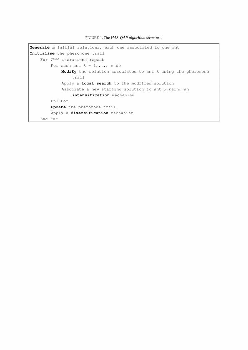
FIGURE 1. The HAS-QAP algorithm structure.

Generate m initial solutions, each one associated to one antInitialise the pheromone trail

For Imax iterations repeatFor each ant k = 1,..., m do

Modify the solution associated to ant k using the pheromonetrail

Apply a local search to the modified solutionAssociate a new starting solution to ant k using an

intensification mechanismEnd ForUpdate the pheromone trailApply a diversification mechanism

End For

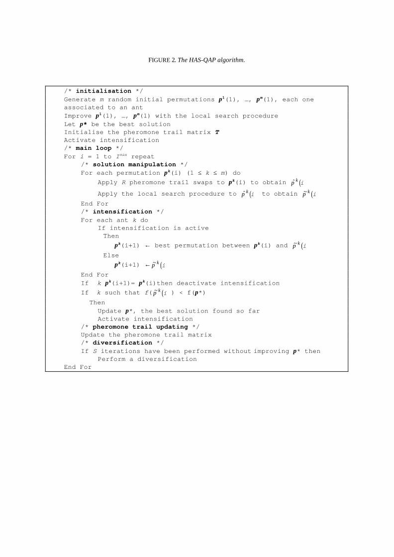
FIGURE 2. The HAS-QAP algorithm.

/* initialisation */Generate m random initial permutations π1(1), …, πm(1), each oneassociated to an antImprove π1(1), …, πm(1) with the local search procedureLet π* be the best solutionInitialise the pheromone trail matrix TActivate intensification/* main loop */For i = 1 to Imax repeat

/* solution manipulation */For each permutation πk(i) (1 ≤ k ≤ m) do Apply R pheromone trail swaps to πk(i) to obtain ( )$π k i

Apply the local search procedure to ( )$π k i to obtain ( )~π k iEnd For/* intensification */For each ant k do

If intensification is activeThen

πk(i+1) ← best permutation between πk(i) and ( )~π k iElse

πk(i+1) ← ( )~π k iEnd ForIf ∀k πk(i+1)= πk(i)then deactivate intensificationIf ∃k such that f( ( )~π k i ) < f(π*)

ThenUpdate π*, the best solution found so farActivate intensification

/* pheromone trail updating */Update the pheromone trail matrix/* diversification */If S iterations have been performed without improving π* then

Perform a diversificationEnd For

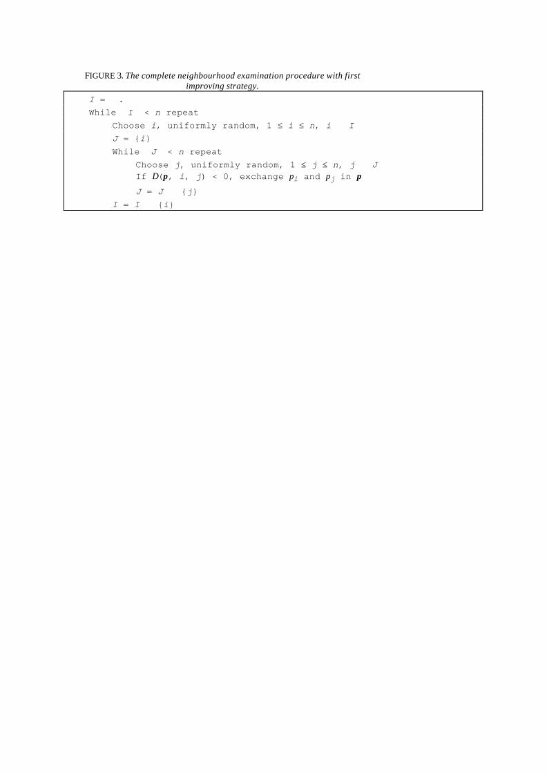
FIGURE 3. The complete neighbourhood examination procedure with firstimproving strategy.

I = ∅.While I < n repeat

Choose i, uniformly random, 1 ≤ i ≤ n, i ∉ IJ = {i}While J < n repeat

Choose j, uniformly random, 1 ≤ j ≤ n, j ∉ JIf ∆(π, i, j) < 0, exchange πi and πj in π

J = J ∪ {j}I = I ∪ {i}

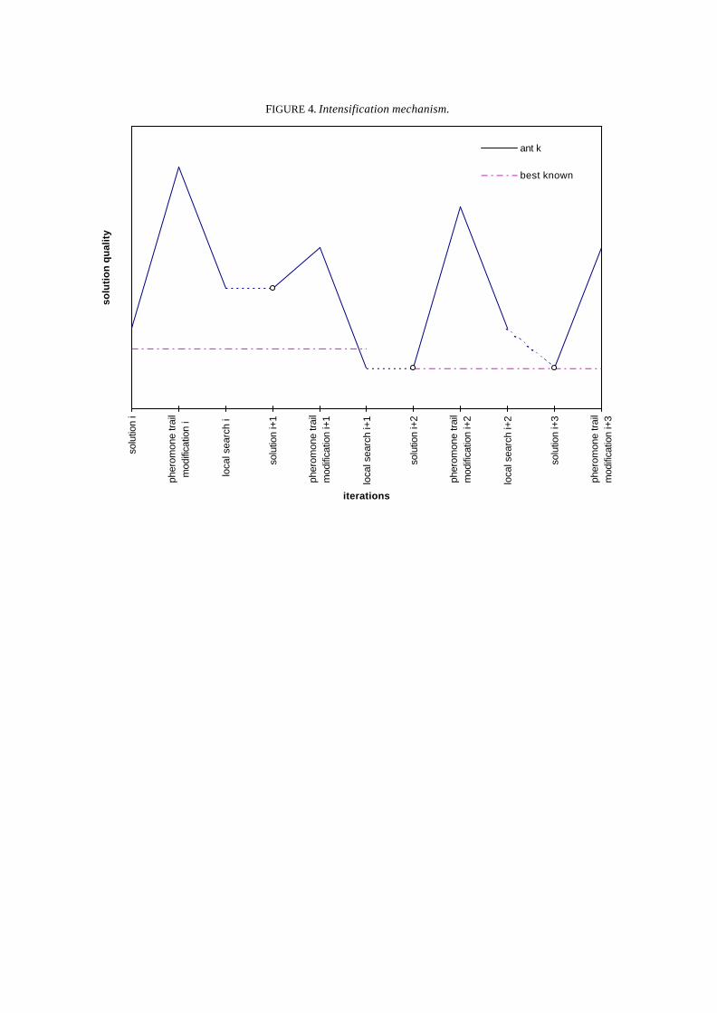
FIGURE 4. Intensification mechanism.

solu

tion

i

pher

omon

e tra

ilm

odifi

catio

n i

loca

l sea

rch

i

solu

tion

i+1

pher

omon

e tra

ilm

odifi

catio

n i+

1

loca

l sea

rch

i+1

solu

tion

i+2

pher

omon

e tra

ilm

odifi

catio

n i+

2

loca

l sea

rch

i+2

solu

tion

i+3

pher

omon

e tra

ilm

odifi

catio

n i+

3

iterations

solu

tio

n q

ual

ity

ant k

best known

TABLE 1. Quality of various heuristic methods for irregular problems and short runs measured in per centabove the best solution value known. Best results are in boldface. Last column reports the computing timegiven to each method that corresponds to the time needed to perform 10 HAS-QAP iterations. All the resultsare averaged over 10 runs.

Problemname

flowdom.

n Best knownvalue

TT RTS SA GH HAS-QAP Seconds

bur26a 2.75 26 5426670 0.208 — 0.185 0.060 0.027 5bur26b 2.75 26 3817852 0.441 — 0.191 0.090 0.106 5bur26c 2.29 26 5426795 0.170 — 0.137 0.004 0.009 5bur26d 2.29 26 3821225 0.249 — 0.379 0.003 0.002 5bur26e 2.55 26 5386879 0.076 — 0.228 0.003 0.004 5bur26f 2.55 26 3782044 0.369 — 0.224 0.006 0.000 5bur26g 2.84 26 10117172 0.078 — 0.139 0.006 0.000 5bur26h 2.84 26 7098658 0.349 — 0.368 0.003 0.001 5chr25a 4.15 25 3796 15.969 16.844 27.139 15.158 15.690 4els19 5.16 19 17212548 21.261 6.714 16.028 0.515 0.923 2kra30a 1.46 30 88900 2.666 2.155 1.813 1.576 1.664 8kra30b 1.46 30 91420 0.478 1.061 1.065 0.451 0.504 9tai20b 3.24 20 122455319 6.700 — 14.392 0.150 0.243 3tai25b 3.03 25 344355646 11.486 — 8.831 0.874 0.133 5tai30b 3.18 30 637117113 13.284 — 13.515 0.952 0.260 9tai35b 3.05 35 283315445 10.165 — 6.935 1.084 0.343 15tai40b 3.13 40 637250948 9.612 — 5.430 1.621 0.280 24tai50b 3.10 50 458821517 7.602 — 4.351 1.397 0.291 50tai60b 3.15 60 608215054 8.692 — 3.678 2.005 0.313 90tai80b 3.21 80 818415043 6.008 — 2.793 2.643 1.108 225

TABLE 2. Quality of various heuristic methods for irregular problems and long runs measured in per centabove the best solution value known. Best results are in boldface. Last column reports the computing timegiven to each method that corresponds to the time needed to perform 100 HAS-QAP iterations (in parenthesisthe average time needed to HAS-QAP to find the best known solution). All the results are averaged over 10runs.

Problemname

n Best known value TT RTS SA GH HAS-QAP Seconds

bur26a 26 5426670 0.0004 — 0.1411 0.0120 0 50 (10)bur26b 26 3817852 0.0032 — 0.1828 0.0219 0 50 (17)bur26c 26 5426795 0.0004 — 0.0742 0 0 50 (3.7)bur26d 26 3821225 0.0015 — 0.0056 0.0002 0 50 (7.9)bur26e 26 5386879 0 — 0.1238 0 0 50 (9.1)bur26f 26 3782044 0.0007 — 0.1579 0 0 50 (3.4)bur26g 26 10117172 0.0003 — 0.1688 0 0 50 (7.7)bur26h 26 7098658 0.0027 — 0.1268 0.0003 0 50 (4.1)chr25a 25 3796 6.9652 9.8894 12.4973 2.6923 3.0822 40els19 19 17212548 0 0.0899 18.5385 0 0 20 (1.6)kra30a 30 88900 0.4702 2.0079 1.4657 0.1338 0.6299 76kra30b 30 91420 0.0591 0.7121 0.1947 0.0536 0.0711 86tai20b 20 122455319 0 — 6.7298 0 0.0905 27tai25b 25 344355646 0.0072 — 1.1215 0 0 50 (12)tai30b 30 637117113 0.0547 — 4.4075 0.0003 0 90 (25)tai35b 35 283315445 0.1777 — 3.1746 0.1067 0.0256 147tai40b 40 637250948 0.2082 — 4.5646 0.2109 0 240 (51)tai50b 50 458821517 0.2943 — 0.8107 0.2142 0.1916 480tai60b 60 608215054 0.3904 — 2.1373 0.2905 0.0483 855tai80b 80 818415043 1.4354 — 1.4386 0.8286 0.6670 2073

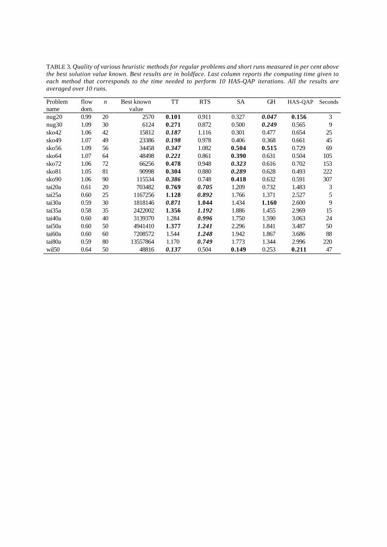
TABLE 3. Quality of various heuristic methods for regular problems and short runs measured in per cent abovethe best solution value known. Best results are in boldface. Last column reports the computing time given toeach method that corresponds to the time needed to perform 10 HAS-QAP iterations. All the results areaveraged over 10 runs.

Problemname

flowdom.

n Best knownvalue

TT RTS SA GH HAS-QAP Seconds

nug20 0.99 20 2570 0.101 0.911 0.327 0.047 0.156 3nug30 1.09 30 6124 0.271 0.872 0.500 0.249 0.565 9sko42 1.06 42 15812 0.187 1.116 0.301 0.477 0.654 25sko49 1.07 49 23386 0.198 0.978 0.406 0.368 0.661 45sko56 1.09 56 34458 0.347 1.082 0.504 0.515 0.729 69sko64 1.07 64 48498 0.221 0.861 0.390 0.631 0.504 105sko72 1.06 72 66256 0.478 0.948 0.323 0.616 0.702 153sko81 1.05 81 90998 0.304 0.880 0.289 0.628 0.493 222sko90 1.06 90 115534 0.386 0.748 0.418 0.632 0.591 307tai20a 0.61 20 703482 0.769 0.705 1.209 0.732 1.483 3tai25a 0.60 25 1167256 1.128 0.892 1.766 1.371 2.527 5tai30a 0.59 30 1818146 0.871 1.044 1.434 1.160 2.600 9tai35a 0.58 35 2422002 1.356 1.192 1.886 1.455 2.969 15tai40a 0.60 40 3139370 1.284 0.996 1.750 1.590 3.063 24tai50a 0.60 50 4941410 1.377 1.241 2.296 1.841 3.487 50tai60a 0.60 60 7208572 1.544 1.248 1.942 1.867 3.686 88tai80a 0.59 80 13557864 1.170 0.749 1.773 1.344 2.996 220wil50 0.64 50 48816 0.137 0.504 0.149 0.253 0.211 47

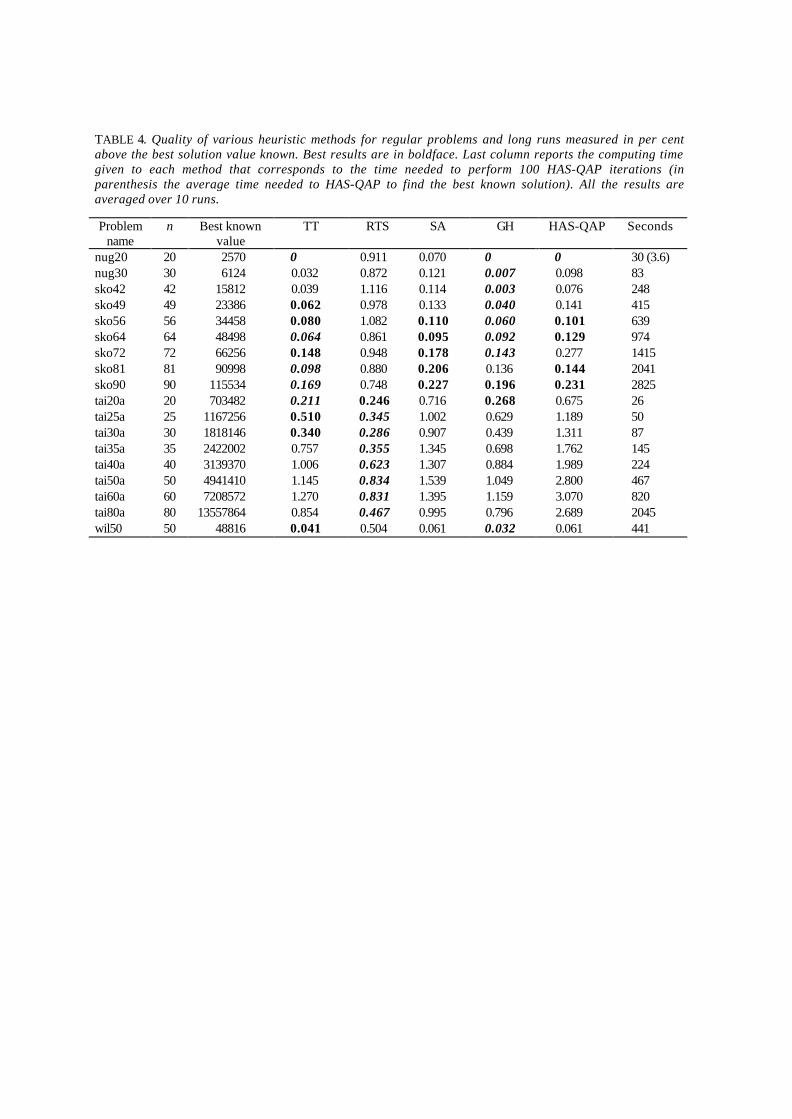
TABLE 4. Quality of various heuristic methods for regular problems and long runs measured in per centabove the best solution value known. Best results are in boldface. Last column reports the computing timegiven to each method that corresponds to the time needed to perform 100 HAS-QAP iterations (inparenthesis the average time needed to HAS-QAP to find the best known solution). All the results areaveraged over 10 runs.

Problemname

n Best knownvalue

TT RTS SA GH HAS-QAP Seconds

nug20 20 2570 0 0.911 0.070 0 0 30 (3.6)nug30 30 6124 0.032 0.872 0.121 0.007 0.098 83sko42 42 15812 0.039 1.116 0.114 0.003 0.076 248sko49 49 23386 0.062 0.978 0.133 0.040 0.141 415sko56 56 34458 0.080 1.082 0.110 0.060 0.101 639sko64 64 48498 0.064 0.861 0.095 0.092 0.129 974sko72 72 66256 0.148 0.948 0.178 0.143 0.277 1415sko81 81 90998 0.098 0.880 0.206 0.136 0.144 2041sko90 90 115534 0.169 0.748 0.227 0.196 0.231 2825tai20a 20 703482 0.211 0.246 0.716 0.268 0.675 26tai25a 25 1167256 0.510 0.345 1.002 0.629 1.189 50tai30a 30 1818146 0.340 0.286 0.907 0.439 1.311 87tai35a 35 2422002 0.757 0.355 1.345 0.698 1.762 145tai40a 40 3139370 1.006 0.623 1.307 0.884 1.989 224tai50a 50 4941410 1.145 0.834 1.539 1.049 2.800 467tai60a 60 7208572 1.270 0.831 1.395 1.159 3.070 820tai80a 80 13557864 0.854 0.467 0.995 0.796 2.689 2045wil50 50 48816 0.041 0.504 0.061 0.032 0.061 441

TABLE 5. Performance of HAS-QAP as a function of thenumber m of ants. Performance is measured as the average ofthe quality values reported in table 1 to 4 for the problemswith n<60. Best results are in boldface.

Number of ants

1 5 10 20Irregular problems

short run 1.99 1.51 1.14 1.30long run 0.63 0.33 0.23 0.34

Regular problems

short run 1.51 1.54 1.59 1.69long run 0.89 0.91 0.85 0.88