Submitted to Operations Researchmanuscript OPRE-2011-06-292

Three ideas for theQuadratic Assignment Problem

Matteo Fischetti, Michele Monaci, Domenico SalvagninDepartment of Information Engineering, University of Padova, Via Gradenigo 6/B, 35121 Padova, Italy,

matteo.fischetti@unipd.it michele.monaci@unipd.it domenico.salvagnin@unipd.it

We address the exact solution of the famous esc instances of the quadratic assignment problem. These areextremely hard instances that remained unsolved—even allowing for a tremendous computing power—byusing all previous techniques from the literature. During this challenging task we found that three ideas wereparticularly useful, and qualified as a breakthrough for our approach. The present paper is about describingthese ideas and their impact in solving esc instances. Our method was able to solve, in a matter of secondsor minutes on a single PC, all easy cases (all esc16* plus esc32e and esc32g). The three previously-unsolvedesc32c, esc32d and esc64a were solved in less than half an hour, in total, on a single PC. We also reportthe solution in about 5 hours of the previously-unsolved tai64c. By using a facility-flow splitting procedure,we were finally able to solve to proven optimality, for the first time, both esc32h (in about 2 hours) as wellas “the big fish” esc128 (to our great surprise, the solution of the latter required just a few seconds on asingle PC).

Key words : integer programming, quadratic assignment problemHistory : Submitted: 11 June 2011

In memory of Jens Clausen

1. Introduction

The NP-hard (and notoriously very difficult in practice) Quadratic Assignment Problem (QAP), inits Koopmans and Beckmann form [Koopmans and Beckmann(1957)], can be sketched as follows;see, e.g., [Cela(1998), Burkard et al.(2009)Burkard, Dell’Amico, and Martello] for details.

We are given a complete directed graph G= (V,A) with n nodes n2 arcs along with a set of nfacilities to be assigned to its nodes. In what follows, indices i, j ∈ V always correspond to nodes,indices f, g ∈N := {1, · · · , n} to facilities, bij ≥ 0 is a given (directed) distance from node i to nodej, afg ≥ 0 is a given required flow from facility f to facility g, and cif is a given fixed cost forassigning facility f to node i. By using binary variables yif = 1 iff facility f is assigned to node i,QAP can be stated as the following quadratic 0-1 problem:

min∑

i∈V∑

f∈N∑

j∈V∑

g∈N afg bij yif yjg +∑

i∈V∑

f∈N cifyif (1)∑i∈V yif = 1 ∀f ∈N (2)∑f∈N yif = 1 ∀i∈ V (3)

yif ∈ {0,1} ∀i∈ V, f ∈N (4)

Notice that the quadratic part of the objective function may hide some linear terms in the prod-ucts affbiiyifyif (as y2if = yif ). Therefore in the following we will always assume, without loss ofgenerality, aff = 0 and bii = 0 for all pairs (i, f), after the update cif := cif + affbii.

It is well known that constraint matrix (2)-(3) is totally unimodular, so optimiz-ing any linear objective function over QAP feasible set is just an easy LP problemsolvable in O(n3) in the worst case, known as the Linear Assignment Problem (LAP)[Burkard et al.(2009)Burkard, Dell’Amico, and Martello].

1

Author: Three ideas for QAP2 Article submitted to Operations Research; manuscript no. OPRE-2011-06-292

In spite of its simple definition, QAP is among the most difficult optimization prob-lems arising in practice, and its study attracted a large amount of research. A QAP fea-ture that challenged us is that a collection of (apparently very small) test-cases is avail-able in the QAPLIB [Burkard et al.(1991)Burkard, Karisch, and Rendl], that cannot be solvedby the current state of the art even by allowing for tremendous computing power. E.g.,an instance with just n = 30 such as tho30 was solved only recently on a distributed grid[Anstreicher et al.(2002)Anstreicher, Brixius, Goux, and Linderoth] and required the equivalent of8,997 days of computation—while many similar instances are still unsolved nowadays.

Among the difficult cases, we concentrated on the so-called esc instances introduced in[Eschermann and Wunderlich(1990)]. As reported in QAPLIB, instances esc32a, esc32b, esc32c,esc32d, esc32h, esc64a, and esc128 are still unsolved by using any published method[Clausen and Perregaard(1997)]. It is fair however to mention that the “What’s new” section ofthe QAPLIB webpage http://www.seas.upenn.edu/qaplib/ states that in January 2011 AxelNyberg and Tapio Westerlund at Abo Akademi University in Finland announced the solution ofesc32a, esc32c, esc32d, esc64a, and tai64c. Instance esc32c took 9 hours on a single PC usingthe commercial solver Gurobi 3.0 (default settings), whereas esc32d took about 35 hours. As faras we know, however, no paper describing this method is available nor circulated in any way, so nocomparison with our own approach can be made.

During our research we tested a number of ideas, and found that three of them were particularlyuseful, and qualified as a breakthrough for our approach. This paper is about describing these ideasand their effect in solving hard esc instances.

Our method was able to solve, in a matter of seconds or minutes on a single PC, all the easycases (all esc16* plus esc32e and esc32g). The three previously-unsolved esc32c, esc32d andesc64a were solved in less than half an hour, in total, on a single quad-core PC. We also reportthe solution of the previously-unsolved tai64c in about 5 hours, on the same PC.

By using a facility-flow splitting procedure, we also succeeded in solving esc128 to provenoptimality—to our great surprise, this task took just a few seconds on our quad-core PC. Accordingto QAPLIB, esc128 is the largest QAP instance ever solved by an exact method. Instance esc32h

was solved as well, and took about 2 hours on the same hardware, whereas for esc32a a very tightlower bound of 128 (out of 130) was proved in a matter of few minutes—the previous best-knownbound was 103.

The paper is organized as follows. We describe the three main steps that proved to be crucialfor the success for our approach, namely: exploiting symmetries (Section 2), designing and solvinga suitable Mixed-Integer Linear Programming (MILP) formulation (Section 3), and exploiting afacility-flow splitting scheme to solve the hardest cases (Section 4). Some conclusions are finallydrawn in Section 5.

An early version of the present paper has been presented at the CPAIOR’11 meeting held inBerlin, May 2011 [Fischetti et al.(2011)Fischetti, Monaci, and Salvagnin].

2. Step One: Exploiting symmetry

In his survey [Anstreicher(2003)], Anstreicher observed that “a careful consideration of the struc-ture present in the larger esc instances is likely to be important in attempts to solve these problemsto optimality”. Indeed, esc instances are known to be highly symmetrical, and important attemptsto deal with this property have been made in the literature, including those in [Kaibel(1998)] and[de Klerk and Sotirov(2010)].

Our approach was to study the symmetry of the QAP instance at hand—rather than that of itsformulation–by addressing the symmetry groups induced by the flow and distance matrices a andb separately.

Author: Three ideas for QAPArticle submitted to Operations Research; manuscript no. OPRE-2011-06-292 3

2.1. Symmetry in the flow matrix

A main source of symmetry for esc instances comes from the presence of what we call clonefacilities—borrowing a concept introduced in [Balas and Fischetti(1993)] for the traveling salesmanproblem.

Definition 1 Assume w.l.o.g. aff = bii = 0 for all i, f . We say that two distinct facilities f and gare clones (w.r.t. matrices a and c) if• afg = agf .• afh = agh and ahf = ahg for all h∈N \ {f, g};• cif = cig for all i∈ V .

Figure 1 Graphical illustration of the first two clone conditions.

Figure 1 gives an illustration of the first two conditions.It is self evident that the presence of clone facilities induces a symmetry in the problem, in

the sense that, for a given clone pair (f, g) and for each i ∈ V , the two variables xif and xig canbe swapped without changing solution cost or feasibility. Of course, one could cope with clonesymmetry by using a modified branching strategy such as isomorphism pruning [Margot(2002)] ororbital branching [Ostrowski et al.(2011)Ostrowski, Linderoth, Rossi, and Smriglio], but can oneactually take advantage of symmetry?

To answer the question above, we observe that the clone property is an equivalence relation thatpartitions the facility set N into m (say) equivalence classes C1, · · · ,Cm that we call clone clusters,each of which plays the role of a different facility type. In what follows, we will always use indexesu, v ∈M := {1, · · · ,m} to denote facility types, and notation θ(f) to identify the type of facilityf ∈N , i.e., f ∈Cθ(f). We also define a shrunken m×m flow matrix a whose entries auv define theflow to be sent from facility type u to facility type v, auu being the (typically nonzero) requiredflow between any two distinct clones in Cu. Analogously, we define a shrunken n×m cost matrixc whose entries ciu give the cost of assigning node i to facility type u. By definition,

aθ(f),θ(g) = afg ∀f, g ∈N, f 6= g (5)

ci,θ(f) = ci,f ∀i∈ V, f ∈N (6)

The above definitions lead themselves to the following rectangular (shrunken) QAP version wheren nodes are to be assigned to m≤ n facility types, the u-th of which needs to allocate µu := |Cu|identical facility copies to different nodes:

min∑

i∈V∑

u∈M∑

j∈V∑

v∈M auv bij xiu xjv +∑

i∈V∑

u∈M ciuxiu (7)

Author: Three ideas for QAP4 Article submitted to Operations Research; manuscript no. OPRE-2011-06-292∑

i∈V xiu = µu ∀u∈M (8)∑u∈M xiu = 1 ∀i∈ V (9)

xiu ∈ {0,1} ∀i∈ V, u∈M. (10)

Note that variables xiu are binary as we cannot assign more than one facility type to each node.

Theorem 1 Model (7)-(10) is a valid reformulation of (1)-(4).

Proof Our order of business is to prove that, for any feasible solution y of (1)-(4), one can definea feasible solution x of (7)-(10) of the same cost, and vice versa.

Because of constraints (3) and (9), the two solutions y and x will be described by specifying, foreach i∈ V , the assigned facility f(i) in y and the facility type u(i) in x.

Given y, solution x is obtained in a straightforward way by defining u(i) := θ(f(i)) for all i.Similarly, given x we define y by choosing f(i) inside Cu(i) so as to never assign a same facilityto two different nodes. This can be easily done, e.g., by initially marking as unused all facilities,and then scanning the nodes i∈ V in an arbitrary order. For each i, choose any unmarked facilityg ∈Cu(i), mark it, and set f(i) := g. Because of (8), this procedure will always produce a feasiblesolution y for (1)-(4).

Note that while the solution x associated to y is unique, there are∏u∈M µu! different solutions

y that can be associated with a given x. In any case, by construction, we have θ(f(i)) = u(i) forall i∈ V .

Let z(y) and z(x) denote the cost of y and x in their respective models. As we are assumingbii = 0 for all i, and because of (5)-(6), we have

z(y) =∑i∈V

∑j∈V \{i}

af(i),f(j) bij +∑i∈V

ci,f(i) = (11)∑i∈V

∑j∈V \{i}

aθ(f(i)),θ(f(j)) bij +∑i∈V

ci,θ(f(i)) = (12)∑i∈V

∑j∈V \{i}

au(i),u(j) bij +∑i∈V

ci,u(i) = z(x) (13)

which concludes the proof. �Clone shrinking can be viewed a generalization of a method proposed in [Kaibel(1998)] for dealing

with the case where k ≤ n facilities have to be assigned to n nodes—as it happens, in particular,in the esc instances. In this case, the QAP instance contains n − k zero (or dummy) facilitiesu such that auv = avu = 0 for all v. Kaibel’s setting can therefore be viewed as a particular caseof our framework arising when shrinking only the cluster induced by the zero facilities. Thoughbeneficial, this latter operation is however not sufficient to remove the symmetry induced by otherclone clusters (if any). For example, instance tai64c has 64 facilities that can be clustered in justtwo classes C1 and C2 with |C1|= 13 and |C2|= 51, and Kaibel’s approach would shrink C2 leavingthe remaining 13 clones untouched.

It is worth observing that one could apply a similar reasoning to matrix b instead of a (as amatter of fact, this is equivalent to just apply a completely-general preprocessing step that swaps aand b while transposing c, an operation that leaves the optimization problem unchanged). However,we have verified that almost no clone exists with respect to the b matrices of the QAPLIB instances.

2.2. Symmetry in the distance matrix

Clones of course do not capture all possible sources of symmetry of a QAP instance, in particularbecause their definition disregards the distance matrix b completely. As a matter of fact, it is wellknown that the symmetry group of b for many QAP instances can lead to very wide orbits.

Author: Three ideas for QAPArticle submitted to Operations Research; manuscript no. OPRE-2011-06-292 5

An extreme case arises when a single orbit of size n exists, meaning that one can alwaysrename the nodes so as to map any node i to any other node j through a node permutationthat leaves b unchanged. This “single b-orbit” property can easily be checked through standardsoftware based e.g., on nauty [McKay(2010)], and we verified it holds true for all esc instances.An important implication is that one can always assume xifix,ufix = 1 for any arbitrary but fixedpair (ifix,ufix) ∈ V ×M . According to our computational experience, imposing such a fixing ina random way is likely to have a negligible impact in the computational effort to optimality, butchoosing the pair in a careful way can be highly beneficial. In our study, we found that choosingxifix,ufix as the one with the larger expected impact for branching (according to the criterion tobe described in the next section) does in fact consistently lead to improved performance.

In any case, fixing a single variable xifix,ufix at the root node does not remove all the symmetriesarising from matrix b, so it is crucial to be able to detect and exploit the residual symmetries.As discussed in the next section, this can be done either by using a sound general-purpose solverthat infers the symmetries from the input model, or by designing an ad-hoc solution method thatderives the symmetries directly from the input data (in particular, from the distance matrix b).

3. Step Two: Mixed-integer linear models and algorithms

Clone shrinking is likely to be beneficial for any QAP solution method applied to instances involvingclone facilities. Our approach was to generate and solve a suitable MILP model, by using both anoff-the-shelf (black-box) MILP solver and an ad-hoc Branch&Cut scheme.

3.1. Choosing a suitable MILP formulation

Most MILP models for QAP work with additional 0-1 variables χiujv = yiuyjv that are used tolinearize the quadratic objective function—the Adams-Johnson model [Adams and Johnson(1994)]being perhaps the best-known such formulation. These kinds of models require Θ(n4) variables andΘ(n3) constraints, so they become huge even for medium-size instances.

As our ultimate goal was to solve esc128, we decided to address more scalable models that do notbecome hopeless for large instances. In particular, we looked for MILP models requiring just O(n2)variables and constraints, and adapted them for our rectangular QAP version. An obvious candidatewas the MILP model credited to Kaufman and Broeckx (KB) [Kaufman and Broeckx(1978)] thatrequires the introduction of just n ·m additional (continuous) variables

wiu = (∑j∈V

∑v∈M

auvbijxjv) xiu (14)

that allow one to formulate the rectangular QAP as the nonlinear problem:

min∑

i∈V∑

u∈M wiu +∑

i∈V∑

u∈M ciuxiu (15)

wiu ≥ (∑

j∈V∑

v∈M auvbijxjv)xiu ∀i∈ V, u∈M (16)

wiu ≥ 0 ∀i∈ V, u∈M (17)

x∈X (18)

where

X := {x : (8)− (10) hold } (19)

denotes the set of feasible solutions. Note that optimizing any linear function over X is just arectangular LAP solvable in O(n3) time.

Author: Three ideas for QAP6 Article submitted to Operations Research; manuscript no. OPRE-2011-06-292

Nonlinear constraints (16) can be linearized as follows. For any given pair (i, u) ∈ V ×M , ourorder of business is to impose the disjunctive condition:

(xiu = 1 and wiu ≥∑j∈V

∑v∈M

auvbijxjv) ∨ (xiu = 0 and wiu ≥ 0) (20)

through linear inequalities that are valid for

Piu := conv(P 0iu ∪P 1

iu)

where

P 1iu := {(x,wiu) : x∈X, xiu = 1, wiu ≥

∑j∈V

∑v∈M

auvbijxjv}

and

P 0iu := {(x,wiu) : x∈X, xiu = 0, wiu ≥ 0}.

Note that, while one can easily optimize any linear function over Piu, the polyhedral structureof Piu is far from trivial and depends on the numerical entries of matrices a and b. E.g., evenfor a toy case with n = m = 5 and auvbij ∈ {0, · · · ,7}, we could verify through software PORTA[Christof(2009)] that Piu has 1693 facets whose definition involves nasty coefficients (up to 84, inabsolute value).

To get a compact formulation, in the basic linearized model one typically looks for a singleconstraint for each pair (i, u), that has the form

wiu ≥ β0 +∑j∈V

∑v∈M

βjvxjv (21)

and capable of imposing (20) whenever x∈X. In the KB model, this is achieved by just replacingthe nonlinear constraints (16) by

wiu ≥∑j∈V

∑v∈M

auvbijxjv −SUMiu(1−xiu) ∀i∈ V, u∈M (22)

where SUMiu :=∑

j∈V∑

v∈M auvbij. This model is however known to be of little use in practicebecause it is heavily based on the big-M constraints (22). As a result, w and x variables have almostno link when x is allowed to be fractional, as it happens in the LP relaxation solved at each nodeof an enumerative solution method. As a matter of fact, it can be proved [Xia and Yuan(2006)]that the root-node bound is always zero with this model when c= 0 (as it happens in most cases).

A first improvement of the KP model has been recently proposed in [Xia and Yuan(2006)]. Forthe sake of completeness, we next rephrase the resulting model for our rectangular QAP version.

For a given pair (i, u)∈ V ×M , let

INC(i, u) :=

{{(j, v) : j = i ∨ v= u} \ {(i, u)} if µu = 1

{(j, v) : j = i} \ {(i, u)} otherwise(23)

be the index set of those variables that are “incompatible” with xiu, i.e., such that, for any x∈X,setting xiu = 1 implies xjv = 0 for all (j, v)∈ INC(i, u). It is immediate to see that xiu = 0 impliesxjv = 1 for at least one (j, v)∈ INC(i, u).

Author: Three ideas for QAPArticle submitted to Operations Research; manuscript no. OPRE-2011-06-292 7

Theorem 2 ([Xia and Yuan(2006)]) The following inequality

wiu ≥∑j∈V

∑v∈M

βjvxjv −MAX(β)(1−xiu)

is valid for Piu, where for all (j, v)∈ V ×M

βjv :=

{0 if (j, v)∈ INC(i, u)

auvbij otherwise(24)

and MAX(β) is the maximum (rectangular) LAP value over β.

Proof The inequality would be obviously valid for P 1iu without zeroing out coefficients βjv for

(j, v) ∈ INC(i, u), that are however immaterial for validity with respect to P 1iu because of the

definition of INC(i, u). Because of the correcting term −MAX(β)(1− xiu), the inequality is alsovalid for P 0

iu, hence the claim. �Note that Xia and Yuan compute MAX(β) without imposing condition xiu = 0, although this

would be mathematically correct and would lead to a possibly improved coefficient.The Xia-Yuan model inherits from the KB one the “big-M trick” of imposing validity for P 0

iu

by using a sufficiently large (in absolute value) negative coefficient for term (1− xiu). However,equations (9) imply that this term is in fact equal to

∑v 6=u xiv, hence one can compute the coefficient

of each xiv (v 6= u) in an independent way, thus obtaining a possibly improved inequality. Moregenerally, for every (i, u) one can easily improve any given valid inequality of the form (21) bylifting, in any given sequence, the coefficients βjv for (j, v) ∈ INC(i, u). For all such (j, v), settingxjv = 1 implies xiu = 0, hence one needs to address validity w.r.t. P 0

iu only, and the lifting coefficientcan easily be computed as

βjv := βjv − (β0 + max{βx : x∈X,xjv = 1}) (25)

Indeed, the value of βjv is immaterial for all x ∈X with xjv = 0. When xjv = 1, instead, validityw.r.t. P 0

iu requires 0≥ β0 + max{βx : x ∈X,xjv = 1}, hence βjv needs to be updated as in (25) soas to guarantee 0 = β0 + max{βx : x∈X,xjv = 1}.

After a number of preliminary (sometimes quite disappointing) tests with different forms of (22),we arrived to the following conclusions:• For each given pair (i, u), a single constraint of the form (22) remains quite weak no matter the

way its coefficients are lifted—its intrinsic big-M nature forces this constraint to become relevantonly when variable xiu is forced to attain a value very close to 1 (e.g., because of branching),whereas any value not very close to 1 deactivates the constraint completely.• The LP relaxation value at the root node is not a discriminating factor (all forms producing

essentially the same LP bound), hence one should prefer a form that best fits the MILP solver,e.g., a sparse form with small coefficients.• For highly-symmetric instances as the esc ones, it is extremely important to choose a for-

mulation that does not hide the instance symmetry. In particular, over-sophisticated formulations(possibly involving clever classes of additional cuts) are perhaps better from a polyhedral point ofview, but are prone to negative side effects such as destroying symmetry—thus making it impos-sible for a general-purpose MILP solver to recognize it and fully exploit it. The lesson learned isthat, in some cases, the simpler the formulation, the more likely it will not introduce nasty sideeffects.

Author: Three ideas for QAP8 Article submitted to Operations Research; manuscript no. OPRE-2011-06-292

We therefore elaborated the Xia-Yuan model with the aim of producing a simple alternative withimproved characteristics—in particular, coefficient sparsity. For each given (i, u), we start with thefollowing reduced-cost version of (21)

wiu ≥MXiu xiu +∑j∈V

∑v∈M

βiu

jvxjv (26)

where MXiu is the value of the maximum LAP with xiu = 1 computed over costs auvbij, and βiu

jv

are the corresponding nonpositive LP reduced costs. To increase sparsity, we reset βiu

jv = 0 forall (j, v) ∈ INC(i, u), an operation that does not affect validity w.r.t. P 1

iu. We then consider all(j, v)∈ INC(i, u), in an arbitrary but fixed sequence, and make the inequality also valid for P 0

iu by

recomputing βiu

jv through lifting.The above considerations are summarized in the following

Theorem 3 For all (i, u)∈ V ×M , inequality (26) is valid for Piu, where MXiu is the maximum

LAP value over costs auvbij when imposing xiu = 1, and βiu

is defined by first taking the (non-

positive) reduced costs associated with MXiu, then resetting βiu

jv = 0 for all (j, v) ∈ INC(i, u), and

finally recomputing βiu

jv for all (j, v) ∈ INC(i, u), in any arbitrary but fixed sequence, by using thelifting formula

βiu

jv :=−max{βiux : x∈X,xjv = 1} ≥ 0. (27)

Proof The inequality is trivially valid for P 1iu as the right-hand side values of (26) and (22)

coincide for all x ∈X with xiu = 1 because of the basic property of LP reduced costs for equally-constrained LPs. As to validity w.r.t. P 0

iu, take any solution x∈X with xiu = 0. As already observed,xiu = 0 implies xjv = 1 for at least one pair (j, v)∈ INC(i, u), so take the last such pair encounteredin the lifting sequence. Because of (27), the right-hand side of (26) becomes nonpositive after lifting,i.e., the inequality is dominated by wiu ≥ 0 and then vanishes, as required. �

A main reason for the use of reduced βjv’s instead of the original βjv’s is that they typicallylead to sparser constraints with smaller coefficient values—both properties being beneficial for thesolution of the model through a MILP solver.

A substantial improvement of the basic KB form, still due to Xia and Yuan [Xia and Yuan(2006)],is the introduction of the additional valid cuts

wiu ≥MNiu xiu, ∀i∈ V, u∈M (28)

where MNiu denotes the minimum rectangular LAP value over costs auvbij when fixing xiu = 1.Note that these cuts do not suffer from the big-M drawback—a small nonzero fractional value forxiu is not able to completely deactivate them. Indeed, the LP relaxation of the model involvingthese cuts gives, at least, the so-called Gilmore-Lawler [Gilmore(1962), Lawler(1963)] bound forQAP—while the original KB model fails to give such bound by a large amount.

A last improvement is proposed in [Zhang et al.(2010)Zhang, Beltran-Royo, and Ma], where theXia-Yuan model is refined to deal implicitly with cuts (28) by working with the shifted variables

σiu :=wiu−MNiu xiu ≥ 0. (29)

After a number of tests, we found that the following new MILP formulation gives the best perfor-mance in our setting.

Author: Three ideas for QAPArticle submitted to Operations Research; manuscript no. OPRE-2011-06-292 9

min∑

i∈V∑

u∈M σiu +∑

i∈V∑

u∈M(ciu +MNiu)xiu (30)

σiu ≥ (MXiu−MNiu)xiu +∑

j∈V∑

v∈M βiu

jvxjv ∀i∈ V, u∈M (31)

σiu ≥ 0, ∀i∈ V, u∈M (32)

x∈X (33)

where, for every (i, u), coefficients MXiu’s and βiu

jv’s are defined as in Theorem 3.As to the variable xifix,ufix possibly fixed to one because of symmetry (see Section 2.2), if any,

we include this fixing in the definition of X so as to tighten the coefficients of all constraints (31).Finally, it is easy to verify that the optimal QAP solution value must be an even integer in case

matrices a, b, c are integer, a and b are symmetric, and c itself is even. In this case, one can slightlyimprove formulation (30)-(33) by rewriting the objective function as just 2z and require

2z =∑i∈V

∑u∈M

σiu +∑i∈V

∑u∈M

(ciu +MNiu)xiu, z integer.

3.2. Use of a general-purpose MILP solver as a black box

Our first quick shot was to write our MILP model (30)-(33) in a file for each esc instance, andto solve it through a black-box commercial MILP solver—IBM ILOG Cplex 12.2 in our case. Wealso included the previously-unsolved instance tai64c in our test-bed because this instance isparticularly suited for our clone-shrinking approach—the number of its facilities being reducedfrom n= 64 to just m= 2.

We provided the black-box solver with a branching-priority input file where the branching pri-ority of variable xiu is a measure of the impact of xiu into our model—and specifically on con-straints (31). This is very much in the spirit of the recent work by Chinneck and co-authors[Patel and Chinneck(2007), Pryor and Chinneck(2011)]. As each constraint (31) has a dominatingcoefficient MXiu−MNiu whose absolute value is typically (integer and) much larger than that ofall other coefficients, we used the score

106(MXiu−MNiu) + 103u+ i

as our branching priority for xiu. Note that variables xiu with MXiu −MNiu = 0, if any, receivethe lowest score, which is very reasonable in that constraint (31) becomes redundant as it requiresσiu ≥ 0 even for xiu = 1, hence σiu = 0 in any optimal solution. This is true, in particular, when uis a zero facility, i.e., auv = avu = 0 for all v.

According to our computational experience, the use of the above priorities has a strong impacton the MILP solver performance, allowing for the solution of instances that are out of reach forthe default—even strong—branching strategies. We are confident that this new branching criterionwill prove quite useful within other solution approaches as well.

Table 1 reports results obtained by using IBM ILOG Cplex 12.2 for solving some easy and hardesc instances (plus tai64c) to proven optimality. These experiments were performed on a quad-core Intel Xeon CPU running at 3.2 GHz under Mac OS 10.6 and equipped with 16GB of RAM.According to our preliminary tests, Cplex typically finds the optimal solutions within negligiblecomputing time for these instances, whereas cuts seem to be counterproductive. Therefore in ourruns Cplex’s cuts and heuristics were disabled, and no upper cutoff was specified on input (weactually used a cutoff of 108 just to help preprocessing to cleanup our model). Instead, the use ofthe most aggressive setting for symmetric reductions (level 5) proved to be highly beneficial.

For all cases, the optimal solution turned out to be of the same value as the best-known onesreported in QAPLIB. All the input (.lp and .ord) files as well as the log’s of these runs are available,on request, from the authors.

Author: Three ideas for QAP10 Article submitted to Operations Research; manuscript no. OPRE-2011-06-292

Table 1 Optimal solutions found by IBM ILOG Cplex 12.2 in interactive mode (8 threads on a quad-core IntelXeon CPU@3.2GHz with 16GB RAM running under MacOS 10.6). Instances marked by ∗ are reported as unsolved

in QAPLIB.

Instance n m OPT time (s) #nodes

esc16a 16 9 68 0.35 4,133esc16b 16 7 292 3.07 71,075esc16c 16 12 160 130.98 2,652,014esc16d 16 12 16 0.51 10,796esc16e 16 8 28 0.05 421esc16f 16 1 0 0.00 0esc16g 16 9 26 0.04 450esc16h 16 5 996 0.23 4,967esc16i 16 10 14 0.18 3,216esc16j 16 7 8 0.03 114esc32c∗ 32 10 642 9,643.82 81,650,962esc32d∗ 32 13 200 2,973.26 12,757,770esc32e 32 6 2 0.04 70esc32g 32 7 6 0.06 597esc64a∗ 64 15 116 509.87 1,206,370tai64c∗ 64 2 1,855,928 18,250.40 1,216,074,081

3.3. Designing an ad-hoc Branch&Cut algorithm

Our next step was the design of an ad-hoc Branch&Cut code, aimed at achieving a better controlon additional cuts, branching strategy, and symmetry breaking.

Local cuts

As far as cuts are concerned, at some branching nodes we generated additional local cuts of theform

σiu ≥ (MN+iu−MNiu)xiu

where MN+iu is defined as MNiu, but takes the current variable fixings into account. In our imple-

mentation, only variables fixed to 1 were considered, hence a very fast O(n) algorithm usingpre-sorted arrays was used to compute MN+

iu—very much in the spirit of the classical Gilmore-Lawler bound computation [Burkard et al.(2009)Burkard, Dell’Amico, and Martello]. As the over-head introduced by the addition of new cuts to the LP (rather than the separation time itself) isquite substantial, we only performed cut generation at the nodes where the number of variablesfixed to 1 was even and in the range [2..16], and we added them to the node relaxation only if thenumber of violated cuts found was not smaller than 5.

Branching strategy

As to branching, we used a standard 2-way branching scheme on a fractional variable xib,ub (say)selected as follows. The input priority file described the previous section was used to select facilityub. As to the choice of ib, we selected the fractional variable that minimizes the quantity∑

(j,v)∈F

aub,vbij

Author: Three ideas for QAPArticle submitted to Operations Research; manuscript no. OPRE-2011-06-292 11

where F is the set of pairs (j, v) for which xjv is fixed to 1 at the current branching node. The

rationale behind this choice is that such a variable gives the smallest contribution to the overall

cost with respect to the fixed variables, and as such it is likely to take value 1 on any “good”

solution in the current subtree. For this reason, fixing it to zero is likely to increase the bound

significantly, thus strengthening the weak zero-branch.

Dealing with residual symmetries

Given the choice of the branching variable, we implemented a specialized orbital branching

and fixing scheme [Ostrowski et al.(2011)Ostrowski, Linderoth, Rossi, and Smriglio], computing

the symmetry groups and orbits associated with the distance matrix b. To ensure correctness of

the resulting code, all Cplex’s symmetry features and dual reductions were deactivated by setting

CPX PARAM SYMMETRY to 0 and CPX PARAM REDUCE to CPX PREREDUCE PRIMALONLY.

The basic idea of our specialized orbital branching implementation is as follows. Given a node

γ of the enumeration tree, let F1(γ)⊂ V be the set of nodes that are fixed to some facility (e.g.,

because of branching). We compute the pointwise-stabilizer stab(F1(γ)) as the subgroup of the

symmetry group of b that keeps each element in F1(γ) fixed. Given a branching variable xiu, we

then compute the orbit Oi with respect to stab(F1(γ)), i.e., the set of nodes that are equivalent to

i according to stab(F1(γ)). Finally, we enforce the branching dichotomy:

(xiu = 1) ∨ (xju = 0 ∀j ∈Oi)

Stabilizers stab(F1(γ)) and orbits Oi could be computed by general purpose tools such as nauty

[McKay(2010)] or saucy [Darga et al.(2008)Darga, Katebi, Liffiton, Markov, and Sakallah]. How-

ever, as long as esc instances are addressed, one can exploit the very special structure of matrix b.

Indeed, bij is defined as the Hamming distance ∆(i, j) between the binary representations of the

two k-bit numbers i− 1 and j − 1, minus 1. As such, any bijective function φ from the set K of

k-bit numbers to itself (a permutation) that preserves the Hamming distance, i.e., such that

∆(φ(i), φ(j)) = ∆(i, j) ∀i, j ∈K,

can be applied to the rows and columns of b, leaving matrix b unchanged. As a matter of fact, it

is known [Anstreicher(2003)] that the following basic operations (and their compositions) preserve

the Hamming distance ∆. Given a k-bit string dk−1 · · ·d1d0:• (flip) flip a given subset T of its bits; e.g., given the 4-bit string d3d2d1d0 = 1001 and the subset

T = {0,2} we obtain d3d2d1d0 = 1100;

• (permute) apply a given bit permutation π; e.g., given the 4-bit string d3d2d1d0 and the bit

permutation (in cycle notation) π= (0,1,2)(3), we obtain d3d1d0d2.

Because of the above symmetries, when selecting the variable xifix,ufix to be fixed to 1, one

can always assume ifix= n, whose associated bit-string is 11 · · ·1. This particular choice removes

all bit flips from the set of feasible operations for computing the stabilizers, so we are left with

permutations only. Note that we are considering permutations of very short bit strings, and the

number of bit permutations is quite small—for our largest instance, esc128, n = 128 requires 7

bits, so there are just 7! = 5,040 possible permutations. We can therefore afford to explicitly pre-

compute and store all possible permutations to be used, at a later time, to compute stabilizers

and orbits at each branching node. To be more specific, at each branching node we start with the

pre-computed list of permutations and filter those that keep each node of F1(γ) fixed. We then

Author: Three ideas for QAP12 Article submitted to Operations Research; manuscript no. OPRE-2011-06-292

compute the orbit Oi of a given node i by just applying the filtered permutations to the binaryrepresentation of i.

Results

Table 2 reports results when using our B&C code on the hardest esc instances of Table 1, on thesame hardware. As expected, our Branch&Cut code outperforms the black-box IBM ILOG Cplex

12.2 solver by a large amount, and it is able to solve esc32c, esc32d and esc64a in less thanhalf an hour in total, on a single quad-core PC. On these instances, the speedup in running timeis about 8×, while the reduction in the number of nodes is approximately 24×.

Table 2 Optimal solutions found by our specialized Branch&Cut code built on top of IBM ILOG Cplex 12.2 (8threads on a quad-core Intel Xeon CPU@3.2GHz with 16GB RAM running under MacOS 10.6). All these instances

are reported as unsolved in QAPLIB.

Instance n OPT time (s) #nodes

esc32c 32 642 1156.00 3,102,322esc32d 32 200 472.68 685,159esc64a 64 116 83.52 143,124

4. Step Three: Exploiting a facility-flow splitting scheme

During our various attempts to solve esc128 we observed the following apparently strange behavior.The best-known upper bound for esc128 is 64, while the Gilmore-Lawler bound is just 2. The

root-node bound for our MILP model is 2 or 4, depending on the choice of the variable that cansafely be fixed to 1 because of symmetry. Depending on the branching order, our enumerativemethod was able to improve this bound quite quickly, reaching lower bound values of about 40after a few minutes of computation if a sound branching order was chosen.1

However, if we deliberately set to zero some nonzero entries of the flow matrix a (chosen in aproper way), a bound of 48 could be proved in about 2 seconds, after having enumerated just2,000 nodes. In other words, we had the evidence that reducing the costs can in fact improve thebound obtained after a fixed amount of enumeration. This is counterintuitive, in that for any givenbranching node the lower bound computed w.r.t. the reduced flow matrix cannot be better thanthat computed w.r.t. the original one, and we do not expect that having a worse bound can helpenumeration.

The explanation is that the modified matrix a induced symmetries that were not present in theoriginal model, hence a large number of nodes could implicitly be pruned because of symmetry(as opposed to bound) considerations. This is particularly true after the application of our clone-shrinking mechanism: two “almost indistinguishable” facilities that could not be shrunk in theoriginal problem, became clones in the reduced one and hence could be collapsed—thus saving ahuge amount of enumeration.

The above considerations prompted us to analyze a facility-flow splitting scheme that is basedon the following theorem. To ease notation, assume c= 0. We denote by QAP(α) the QAP instance(before clone shrinking) defined by flow matrix α, and by opt(α) its optimal solution value.

1 As an exercise, we tried 200 random perturbation of our branching priority order: the bound available after 50,000enumeration nodes using IBM ILOG Cplex 12.2 in interactive mode ranged from just 4 to 46.

Author: Three ideas for QAPArticle submitted to Operations Research; manuscript no. OPRE-2011-06-292 13

Theorem 4 Let a1 and a2 be nonnegative matrices such that a= a1 +a2. Then opt(a1)+opt(a2)≤opt(a).

Proof Let y any feasible solution to model (1)-(4). Then∑i∈V

∑u∈M

∑j∈V

∑v∈M

auv bij yiu yjv =

∑i∈V

∑u∈M

∑j∈V

∑v∈M

a1uv bij yiu yjv +∑i∈V

∑u∈M

∑j∈V

∑v∈M

a2uv bij yiu yjv

i.e., the cost of y in QAP(a) is equal to the cost of y in QAP(a1) plus its cost in QAP(a2). Theinequality sign in opt(a1)+opt(a2)≤ opt(a) comes from the fact that we do not impose the optimalsolution of QAP(a) to be coincident with the optimal solutions of QAP(a1) and QAP(a2)—imposingthis condition would lead to an exact variable-splitting reformulation. �

Theorem 4 remains obviously valid for nonnegative flow matrices a1 and a2 such that a≥ a1 +a2.In addition, the decomposition scheme can be iterated any number of times.

At first glance, computing a lower bound on the optimal QAP value by solving two QAP instancesof the same size does not seem a clever idea. However, as already observed, for an effective solutionof a MILP instance through an enumerative method, the structure of the instance matters evenmore than its size, so the real question is: Can we find a clever way to define two nonnegative flowmatrices a1 and a2 := a−a1 so as to obtain a structure that simplifies the exact solution process ofboth QAP(a1) and QAP(a2)? We tested two possible answers to the above question, both aimedat increasing the number of clones in both a1 and a2 (we assume a integer, as it is the case for allQAPLIB instances):

(i) define a1 as the support of a, i.e., a1fg := min{afg,1}(ii) select a facility subset S ⊂N and define a1fg := 0 if f ∈ S or g ∈ S, a1fg := afg otherwise.The rationale of criterion (i) is clear: if we only distinguish between zero and nonzero entries in

a1 we increase the occurrence of clones, whereas a2 becomes sparser than a and hence is likely tocontain more clones.

Analogously, by using criterion (ii) all the facilities in S become zero-facilities w.r.t. a1 andhence will be shrunk, whereas a2 will be significantly sparser than a (and thus likely to containmore clones). In order to have a tight bound, a clever choice is to select S as a facility subset thatcontains no zero-facilities w.r.t. a, and such that the total flow passing through the cut (S,N \S)is as close to zero as possible.

By applying splitting criterion (i) to instance esc32h we were able to solve both QAP(a1)and QAP(a2) quite efficiently (on our PC, the B&C code took 4 and 7,795 seconds for the enu-meration of 39,183 and 37,114,507 nodes, respectively), obtaining a lower bound of opt(a1) +opt(a2) = 340 + 98 = 438 that is equal to the value of the best-know feasible solution reported in[Burkard et al.(1991)Burkard, Karisch, and Rendl], thus proving its optimality.

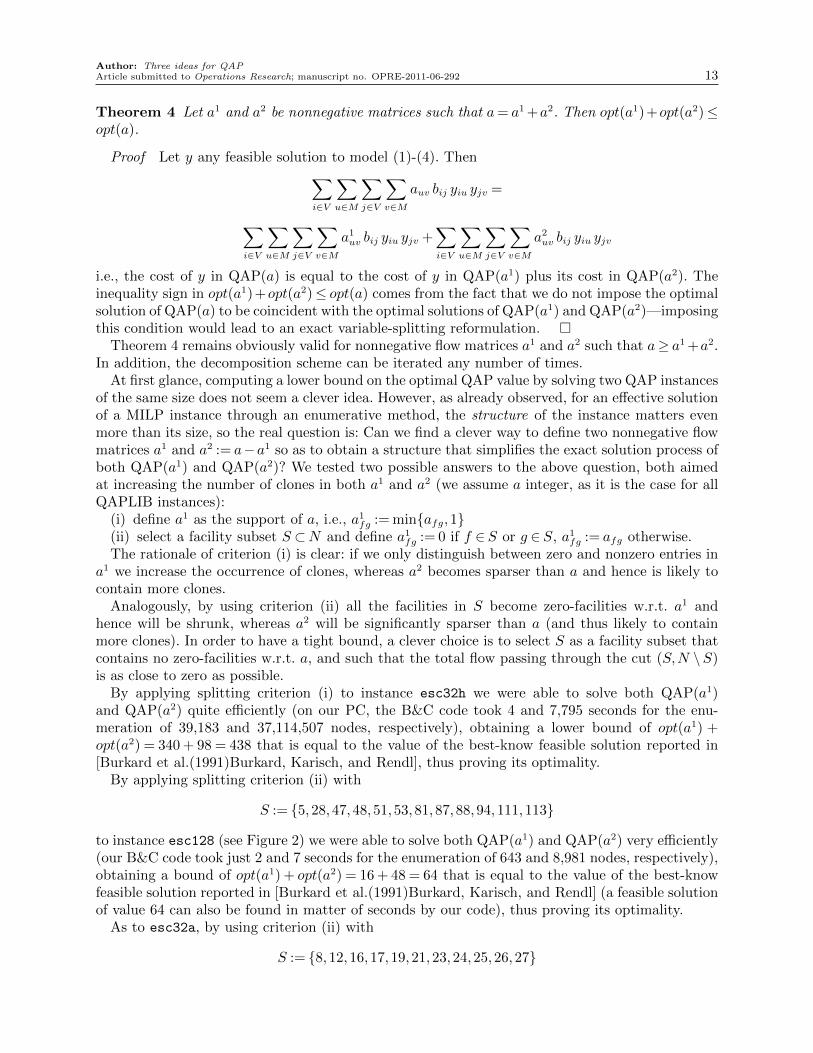
By applying splitting criterion (ii) with

S := {5,28,47,48,51,53,81,87,88,94,111,113}

to instance esc128 (see Figure 2) we were able to solve both QAP(a1) and QAP(a2) very efficiently(our B&C code took just 2 and 7 seconds for the enumeration of 643 and 8,981 nodes, respectively),obtaining a bound of opt(a1) + opt(a2) = 16 + 48 = 64 that is equal to the value of the best-knowfeasible solution reported in [Burkard et al.(1991)Burkard, Karisch, and Rendl] (a feasible solutionof value 64 can also be found in matter of seconds by our code), thus proving its optimality.

As to esc32a, by using criterion (ii) with

S := {8,12,16,17,19,21,23,24,25,26,27}

Author: Three ideas for QAP14 Article submitted to Operations Research; manuscript no. OPRE-2011-06-292

5

1416

28

31

33

35

36

40

42

43

47

48

5153

6264

66

69

71

73

75

77

79

80

81

87

88

94

111

113

Figure 2 Support of the flow matrix a for instance esc128 (zero facilities not shown).

(see Figure 3) we could again solve both QAP(a1) and QAP(a2) very efficiently (6 and 45seconds for the enumeration of 19,247 and 201,178 nodes, respectively), obtaining a verytight bound of opt(a1) + opt(a2) = 68 + 60 = 128. As the best-known solution reported in[Burkard et al.(1991)Burkard, Karisch, and Rendl] has a value of 130, the (even) optimal solutionvalue must be equal to either 128 or 130.

Table 3 summarizes the results obtained through our facility-flow splitting scheme. Computingtimes (in seconds) and numbers of nodes give the sum over the two runs of our Branch&Cut codeto solve QAP(a1) and QAP(a2). Computing times do not include the time needed to generate andwrite the input MILP model files—this task required negligible time for esc32*, and about oneminute for esc128.

5. Conclusions and future work

Three ideas toward the solution of hard QAP instances have been presented and evaluated exper-imentally on hard cases. To our pleasant surprise, at least for esc instances these ideas producedvery good computational results even when embedded in a very basic solution scheme using off-the-shelf MILP technology.

Author: Three ideas for QAPArticle submitted to Operations Research; manuscript no. OPRE-2011-06-292 15

1

2

3

4

5

6

8

9

10

11

12

13

14

15

16

17

18

19

21

22

23

24

25

26

27

Figure 3 Support of the flow matrix a for instance esc32a (zero facilities not shown).

Table 3 Results obtained by our specialized Branch&Cut code through facility-flow splitting (8 threads on aquad-core Intel Xeon CPU@3.2GHz with 16GB RAM running under MacOS 10.6). All these instances are reported

as unsolved in QAPLIB.

Instance n UB LB time (s) #nodes

esc32a 32 130 60+68=128 51.16 220,425esc32h 32 438 340+96=438 7,799.90 37,153,690esc128 128 64 48+16= 64 9.63 9,624

We were able to solve to proven optimality all esc instances, with the only exception of esc32a(for which we proved a bound of 128 out of 130) and esc32b. In particular we solved, for the firsttime and in a matter of seconds, the “big fish” esc128—this is the largest QAPLIB instance eversolved to proven optimality [Burkard et al.(1991)Burkard, Karisch, and Rendl].

Future work should address the solution of the still-unsolved esc instances, and also the appli-cability of our ideas to other classes of still-unsolved QAP instances.

AcknowledgmentsResearch supported by the Progetto di Ateneo on “Computational Integer Programming” of the University

of Padova. We thank Gianfranco Bilardi and Enoch Peserico for the use of the computers of the Center ofExcellence “Scientific and Engineering Applications of Advanced Computing Paradigms”.

References[Adams and Johnson(1994)] Adams, W.P., T.A. Johnson. 1994. Improved linear programming-based lower bounds for

the quadratic assignment problem. Proceedings of the DIMACS Workshop on Quadratic Assignment Problems,DIMACS Series in Discrete Mathematics and Theoretical Computer Science, vol. 16. American MathematicalSociety, 43–75.

[Anstreicher(2003)] Anstreicher, K. M. 2003. Recent advances in the solution of quadratic assignment problems.Mathematical Programming 97 27–42.

Author: Three ideas for QAP16 Article submitted to Operations Research; manuscript no. OPRE-2011-06-292

[Anstreicher et al.(2002)Anstreicher, Brixius, Goux, and Linderoth] Anstreicher, K.M., N.W. Brixius, J.-P. Goux,J. Linderoth. 2002. Solving large quadratic assignment problems on computational grids. Mathematical Program-ming 91 563–588.

[Balas and Fischetti(1993)] Balas, E., M. Fischetti. 1993. A lifting procedure for the asymmetric traveling salesmanpolytope and a large new class of facets. Mathematical Programming 58 325–352.

[Burkard et al.(2009)Burkard, Dell’Amico, and Martello] Burkard, R.E., M. Dell’Amico, S. Martello. 2009. Assign-ment Problems. SIAM. URL http://www.ec-securehost.com/SIAM/OT106.html.

[Burkard et al.(1991)Burkard, Karisch, and Rendl] Burkard, R.E., S. Karisch, F. Rendl. 1991. QAPLIB – A quadraticassignment problem library. European Journal of Operational Research 55 115–119. URL http://www.seas.upenn.edu/qaplib/.

[Cela(1998)] Cela, E. 1998. The quadratic assignment problem: Theory and algorithms. Kluwer Academic Publishers,Dordrecht, The Netherlands. URL http://www.ams.org/mathscinet-getitem?mr=99a%3a90001.

[Christof(2009)] Christof, T. 2009. Porta. URL http://typo.zib.de/opt-long_projects/Software/Porta/.

[Clausen and Perregaard(1997)] Clausen, J., M. Perregaard. 1997. Solving large quadratic assignment problems inparallel. Computational Optimization and Applications 8 111–127.

[Darga et al.(2008)Darga, Katebi, Liffiton, Markov, and Sakallah] Darga, P. T., H. Katebi, M. Liffiton, I. Markov,K. Sakallah. 2008. Saucy. URL http://vlsicad.eecs.umich.edu/BK/SAUCY/.

[de Klerk and Sotirov(2010)] de Klerk, E., R. Sotirov. 2010. Exploiting group symmetry in semidefinite programmingrelaxations of the quadratic assignment problem. Mathematical Programming 122 225–246.

[Eschermann and Wunderlich(1990)] Eschermann, B., H. J. Wunderlich. 1990. Optimized synthesis of self-testablefinite state machines. 20th International Symposium on Fault-Tolerant Computing (FFTCS 20). 390–397.

[Fischetti et al.(2011)Fischetti, Monaci, and Salvagnin] Fischetti, M., M. Monaci, D. Salvagnin. 2011. Three ideasfor the quadratic assignment problem. CPAIOR 2011, Late Breaking Abstracts. ZIB report 11-20, 9–13. URLhttp://cpaior2011.zib.de/downloads/CPAIOR2011_abstracts.pdf.

[Gilmore(1962)] Gilmore, P.C. 1962. Optimal and suboptimal algorithms for the quadratic assignment problem. SIAMJournal on Applied Mathematics 14 305–313.

[Kaibel(1998)] Kaibel, V. 1998. Polyhedral combinatorics of quadratic assignment problems with less objects thanlocations. R. Bixby, E. Boyd, R. Rıos-Mercado, eds., Integer Programming and Combinatorial Optimization,Lecture Notes in Computer Science, vol. 1412. Springer Berlin / Heidelberg, 409–422.

[Kaufman and Broeckx(1978)] Kaufman, L., F. Broeckx. 1978. An algorithm for the quadratic assignment problemusing Benders’ decomposition. European Journal of Operational Research 2 204–211.

[Koopmans and Beckmann(1957)] Koopmans, T.C., M.J. Beckmann. 1957. Assignment problems and the location ofeconomic activities. Econometrica 25 53–76.

[Lawler(1963)] Lawler, E.L. 1963. The quadratic assignment problem. Management Science 9 586–599.

[Margot(2002)] Margot, F. 2002. Pruning by isomorphism in branch-and-cut. Mathematical Programming 94 71–90.

[McKay(2010)] McKay, B.D. 2010. Nauty users guide (version 2.4). Technical report, Dept. Comp. Sci., AustralianNational University.

[Ostrowski et al.(2011)Ostrowski, Linderoth, Rossi, and Smriglio] Ostrowski, J., J. Linderoth, F. Rossi, S. Smriglio.2011. Orbital branching. Mathematical Programming 126 147–178.

[Patel and Chinneck(2007)] Patel, J., J.W. Chinneck. 2007. Active-constraint variable ordering for faster feasibilityof mixed integer linear programs. Mathematical Programming 3 445–474.

[Pryor and Chinneck(2011)] Pryor, J., J.W. Chinneck. 2011. Faster integer-feasibility in mixed-integer linear pro-grams by branching to force change. Computers & OR 38 1143–1152.

[Xia and Yuan(2006)] Xia, Y., Y.X. Yuan. 2006. A new linearization method for quadratic assignment problem.Optimization Methods and Software 21 803–816.

[Zhang et al.(2010)Zhang, Beltran-Royo, and Ma] Zhang, H., C. Beltran-Royo, L. Ma. 2010. Solving the quadraticassignment problem by means of general purpose mixed integer linear programming. URL http://www.optimization-online.org/DB_HTML/2010/05/2622.html.