· Anders Vretblad Department of Mathematics Uppsala University Box 480 SE-751 06 Uppsala Sweden...
282
Transcript of · Anders Vretblad Department of Mathematics Uppsala University Box 480 SE-751 06 Uppsala Sweden...


Graduate Texts in Mathematics 223Editorial Board
S. Axler F.W. Gehring K.A. Ribet

This page intentionally left blank

Anders Vretblad
Fourier Analysis andIts Applications

Anders VretbladDepartment of MathematicsUppsala UniversityBox 480SE-751 06 [email protected]
Editorial Board:S. Axler F.W. Gehring K.A. RibetMathematics Department Mathematics Department Mathematics DepartmentSan Francisco State East Hall University of California,
University University of Michigan BerkeleySan Francisco, CA 94132 Ann Arbor, MI 48109 Berkeley, CA 94720-3840USA USA [email protected] [email protected] [email protected]
Mathematics Subject Classification (2000): 42-01
Library of Congress Cataloging-in-Publication DataVretblad, Anders.
Fourier analysis and its applications / Anders Vretblad.p. cm.
Includes bibliographical references and index.ISBN 0-387-00836-5 (hc. : alk. paper)1. Fourier analysis. I. Title.
QA403.5. V74 2003515′2433—dc21 2003044941
ISBN 0-387-00836-5 Printed on acid-free paper.
2003 Springer-Verlag New York, Inc.All rights reserved. This work may not be translated or copied in whole or in part without thewritten permission of the publisher (Springer-Verlag New York, Inc., 175 Fifth Avenue, New York,NY 10010, USA), except for brief excerpts in connection with reviews or scholarly analysis. Usein connection with any form of information storage and retrieval, electronic adaptation, computersoftware, or by similar or dissimilar methodology now known or hereafter developed is forbidden.The use in this publication of trade names, trademarks, service marks, and similar terms, even ifthey are not identified as such, is not to be taken as an expression of opinion as to whether or notthey are subject to proprietary rights.
Printed in the United States of America.
9 8 7 6 5 4 3 2 1 SPIN 10920442
www.springer-ny.com
Springer-Verlag New York Berlin HeidelbergA member of BertelsmannSpringer Science+Business Media GmbH

To
Yngve Domar,
my teacher, mentor, and friend

This page intentionally left blank

Preface
The classical theory of Fourier series and integrals, as well as Laplace trans-forms, is of great importance for physical and technical applications, andits mathematical beauty makes it an interesting study for pure mathemati-cians as well. I have taught courses on these subjects for decades to civilengineering students, and also mathematics majors, and the present volumecan be regarded as my collected experiences from this work.
There is, of course, an unsurpassable book on Fourier analysis, the trea-tise by Katznelson from 1970. That book is, however, aimed at mathemat-ically very mature students and can hardly be used in engineering courses.On the other end of the scale, there are a number of more-or-less cookbook-styled books, where the emphasis is almost entirely on applications. I havefelt the need for an alternative in between these extremes: a text for theambitious and interested student, who on the other hand does not aspire tobecome an expert in the field. There do exist a few texts that fulfill theserequirements (see the literature list at the end of the book), but they donot include all the topics I like to cover in my courses, such as Laplacetransforms and the simplest facts about distributions.
The reader is assumed to have studied real calculus and linear algebraand to be familiar with complex numbers and uniform convergence. Onthe other hand, we do not require the Lebesgue integral. Of course, thissomewhat restricts the scope of some of the results proved in the text, butthe reader who does master Lebesgue integrals can probably extrapolatethe theorems. Our ambition has been to prove as much as possible withinthese restrictions.
viii
Some knowledge of the simplest distributions, such as point masses anddipoles, is essential for applications. I have chosen to approach this mat-ter in two separate ways: first, in an intuitive way that may be sufficientfor engineering students, in star-marked sections of Chapter 2 and sub-sequent chapters; secondly, in a more strict way, in Chapter 8, where atleast the fundaments are given in a mathematically correct way. Only theone-dimensional case is treated. This is not intended to be more than themerest introduction, to whet the reader’s appetite.
Acknowledgements. In my work I have, of course, been inspired by exist-ing literature. In particular, I want to mention a book by Arne Broman,Introduction to Partial Differential Equations... (Addison–Wesley, 1970), acompendium by Jan Petersson of the Chalmers Institute of Technology inGothenburg, and also a compendium from the Royal Institute of Technol-ogy in Stockholm, by Jockum Aniansson, Michael Benedicks, and KarimDaho. I am grateful to my colleagues and friends in Uppsala. First of allProfessor Yngve Domar, who has been my teacher and mentor, and whointroduced me to the field. The book is dedicated to him. I am also partic-ularly indebted to Gunnar Berg, Christer O. Kiselman, Anders Kallstrom,Lars-Ake Lindahl, and Lennart Salling. Bengt Carlsson has helped withideas for the applications to control theory. The problems have been workedand re-worked by Jonas Bjermo and Daniel Domert. If any incorrect an-swers still remain, the blame is mine.
Finally, special thanks go to three former students at Uppsala University,Mikael Nilsson, Matthias Palmer, and Magnus Sandberg. They used anearly version of the text and presented me with very constructive criticism.This actually prompted me to pursue my work on the text, and to translateit into English.
Uppsala, Sweden Anders VretbladJanuary 2003
Contents
Preface vii
1 Introduction 11.1 The classical partial differential equations . . . . . . . . . . 11.2 Well-posed problems . . . . . . . . . . . . . . . . . . . . . . 31.3 The one-dimensional wave equation . . . . . . . . . . . . . . 51.4 Fourier’s method . . . . . . . . . . . . . . . . . . . . . . . . 9
2 Preparations 152.1 Complex exponentials . . . . . . . . . . . . . . . . . . . . . 152.2 Complex-valued functions of a real variable . . . . . . . . . 172.3 Cesaro summation of series . . . . . . . . . . . . . . . . . . 202.4 Positive summation kernels . . . . . . . . . . . . . . . . . . 222.5 The Riemann–Lebesgue lemma . . . . . . . . . . . . . . . . 252.6 *Some simple distributions . . . . . . . . . . . . . . . . . . 272.7 *Computing with δ . . . . . . . . . . . . . . . . . . . . . . . 32
3 Laplace and Z transforms 393.1 The Laplace transform . . . . . . . . . . . . . . . . . . . . . 393.2 Operations . . . . . . . . . . . . . . . . . . . . . . . . . . . 423.3 Applications to differential equations . . . . . . . . . . . . . 473.4 Convolution . . . . . . . . . . . . . . . . . . . . . . . . . . . 533.5 *Laplace transforms of distributions . . . . . . . . . . . . . 573.6 The Z transform . . . . . . . . . . . . . . . . . . . . . . . . 60

x Contents
3.7 Applications in control theory . . . . . . . . . . . . . . . . . 67Summary of Chapter 3 . . . . . . . . . . . . . . . . . . . . . . . . 70
4 Fourier series 734.1 Definitions . . . . . . . . . . . . . . . . . . . . . . . . . . . . 734.2 Dirichlet’s and Fejer’s kernels; uniqueness . . . . . . . . . . 804.3 Differentiable functions . . . . . . . . . . . . . . . . . . . . . 844.4 Pointwise convergence . . . . . . . . . . . . . . . . . . . . . 864.5 Formulae for other periods . . . . . . . . . . . . . . . . . . . 904.6 Some worked examples . . . . . . . . . . . . . . . . . . . . . 914.7 The Gibbs phenomenon . . . . . . . . . . . . . . . . . . . . 934.8 *Fourier series for distributions . . . . . . . . . . . . . . . . 96Summary of Chapter 4 . . . . . . . . . . . . . . . . . . . . . . . . 100
5 L2 Theory 1055.1 Linear spaces over the complex numbers . . . . . . . . . . . 1055.2 Orthogonal projections . . . . . . . . . . . . . . . . . . . . . 1105.3 Some examples . . . . . . . . . . . . . . . . . . . . . . . . . 1145.4 The Fourier system is complete . . . . . . . . . . . . . . . . 1195.5 Legendre polynomials . . . . . . . . . . . . . . . . . . . . . 1235.6 Other classical orthogonal polynomials . . . . . . . . . . . . 127Summary of Chapter 5 . . . . . . . . . . . . . . . . . . . . . . . . 130
6 Separation of variables 1376.1 The solution of Fourier’s problem . . . . . . . . . . . . . . . 1376.2 Variations on Fourier’s theme . . . . . . . . . . . . . . . . . 1396.3 The Dirichlet problem in the unit disk . . . . . . . . . . . . 1486.4 Sturm–Liouville problems . . . . . . . . . . . . . . . . . . . 1536.5 Some singular Sturm–Liouville problems . . . . . . . . . . . 159Summary of Chapter 6 . . . . . . . . . . . . . . . . . . . . . . . . 160
7 Fourier transforms 1657.1 Introduction . . . . . . . . . . . . . . . . . . . . . . . . . . . 1657.2 Definition of the Fourier transform . . . . . . . . . . . . . . 1667.3 Properties . . . . . . . . . . . . . . . . . . . . . . . . . . . . 1687.4 The inversion theorem . . . . . . . . . . . . . . . . . . . . . 1717.5 The convolution theorem . . . . . . . . . . . . . . . . . . . . 1767.6 Plancherel’s formula . . . . . . . . . . . . . . . . . . . . . . 1807.7 Application 1 . . . . . . . . . . . . . . . . . . . . . . . . . . 1827.8 Application 2 . . . . . . . . . . . . . . . . . . . . . . . . . . 1857.9 Application 3: The sampling theorem . . . . . . . . . . . . . 1877.10 *Connection with the Laplace transform . . . . . . . . . . . 1887.11 *Distributions and Fourier transforms . . . . . . . . . . . . 190Summary of Chapter 7 . . . . . . . . . . . . . . . . . . . . . . . . 192

Contents xi
8 Distributions 1978.1 History . . . . . . . . . . . . . . . . . . . . . . . . . . . . . 1978.2 Fuzzy points – test functions . . . . . . . . . . . . . . . . . 2008.3 Distributions . . . . . . . . . . . . . . . . . . . . . . . . . . 2038.4 Properties . . . . . . . . . . . . . . . . . . . . . . . . . . . . 2068.5 Fourier transformation . . . . . . . . . . . . . . . . . . . . . 2138.6 Convolution . . . . . . . . . . . . . . . . . . . . . . . . . . . 2188.7 Periodic distributions and Fourier series . . . . . . . . . . . 2208.8 Fundamental solutions . . . . . . . . . . . . . . . . . . . . . 2218.9 Back to the starting point . . . . . . . . . . . . . . . . . . . 223Summary of Chapter 8 . . . . . . . . . . . . . . . . . . . . . . . . 224
9 Multi-dimensional Fourier analysis 2279.1 Rearranging series . . . . . . . . . . . . . . . . . . . . . . . 2279.2 Double series . . . . . . . . . . . . . . . . . . . . . . . . . . 2309.3 Multi-dimensional Fourier series . . . . . . . . . . . . . . . . 2339.4 Multi-dimensional Fourier transforms . . . . . . . . . . . . . 236
Appendices
A The ubiquitous convolution 239
B The discrete Fourier transform 243
C Formulae 247C.1 Laplace transforms . . . . . . . . . . . . . . . . . . . . . . . 247C.2 Z transforms . . . . . . . . . . . . . . . . . . . . . . . . . . 250C.3 Fourier series . . . . . . . . . . . . . . . . . . . . . . . . . . 251C.4 Fourier transforms . . . . . . . . . . . . . . . . . . . . . . . 252C.5 Orthogonal polynomials . . . . . . . . . . . . . . . . . . . . 254
D Answers to selected exercises 257
E Literature 265
Index 267

This page intentionally left blank

1Introduction
1.1 The classical partial differential equations
In this introductory chapter, we give a brief survey of three main types ofpartial differential equations that occur in classical physics. We begin byestablishing some convenient notation.
Let Ω be a domain (an open and connected set) in three-dimensionalspace R3, and let T be an open interval on the time axis. By Ck(Ω), resp.Ck(Ω × T ), we mean the set of all real-valued functions u(x, y, z), resp.u(x, y, z, t), with all their partial derivatives of order up to and includingk defined and continuous in the respective regions. It is often practical tocollect the three spatial coordinates (x, y, z) in a vector x and describe thefunctions as u(x), resp. u(x, t). By ∆ we mean the Laplace operator
∆ = ∇2 :=∂2
∂x2 +∂2
∂y2 +∂2
∂z2 .
Partial derivatives will mostly be indicated by subscripts, e.g.,
ut =∂u
∂t, uyx =
∂2u
∂x∂y.
The first equation to be considered is called the heat equation or thediffusion equation:
∆u =1a2
∂u
∂t, (x, t) ∈ Ω × T.

2 1. Introduction
As the name indicates, this equation describes conduction of heat in ahomogeneous medium. The temperature at the point x at time t is givenby u(x, t), and a is a constant that depends on the conducting propertiesof the medium. The equation can also be used to describe various processesof diffusion, e.g., the diffusion of a dissolved substance in the solvent liquid,neutrons in a nuclear reactor, Brownian motion, etc.
The equation represents a category of second-order partial differentialequations that is traditionally categorized as parabolic. Characteristically,these equations describe non-reversible processes, and their solutions arehighly regular functions (of class C∞).
In this book, we shall solve some special problems for the heat equa-tion. We shall be dealing with situations where the spatial variable can beregarded as one-dimensional: heat conduction in a homogeneous rod, com-pletely isolated from the exterior (except possibly at the ends of the rod).In this case, the equation reduces to
uxx =1a2 ut .
The wave equation has the form
∆u =1c2∂2u
∂t2, (x, t) ∈ Ω × T.
where c is a constant. This equation describes vibrations in a homogeneousmedium. The value u(x, t) is interpreted as the deviation at time t fromthe position at rest of the point with rest position given by x.
The equation is a case of hyperbolic equations. Equations of this categorytypically describe reversible processes (the past can be deduced from thepresent and future by “reversion of time”). Sometimes it is even suitableto allow solutions for which the partial derivatives involved in the equationdo not exist in the usual sense. (Think of shock waves such as the sonicbangs that occur when an aeroplane goes supersonic.) We shall be studyingthe one-dimensional wave equation later on in the book. This case can, forinstance, describe the motion of a vibrating string.
Finally we consider an equation that does not involve time. It is calledthe Laplace equation and it looks simply like this:
∆u = 0.
It occurs in a number of physical situations: as a special case of the heatequation, when one considers a stationary situation, a steady state, thatdoes not depend on time (so that ut = 0); as an equation satisfied by thepotential of a conservative force; and as an object of considerable purelymathematical interest. Together with the closely related Poisson equa-tion, ∆u(x) = F (x), where F is a known function, it is typical of equations

1.2 Well-posed problems 3
classified as elliptic. The solutions of the Laplace equation are very regularfunctions: not only do they have derivatives of all orders, there are even cer-tain possibilities to reconstruct the whole function from its local behaviournear a single point. (If the reader is familiar with analytic functions, thisshould come as no news in the two-dimensional case: then the solutionsare harmonic functions that can be interpreted (locally) as real parts ofanalytic functions.)
The names elliptic, parabolic, and hyperbolic are due to superficial sim-ilarities in the appearance of the differential equations and the equationsof conics in the plane. The precise definitions of the different types are asfollows: The unknown function is u = u(x) = u(x1, x2, . . . , xm). The equa-tions considered are linear; i.e., they can be written as a sum of terms equalto a known function (which can be identically zero), where each term inthe sum consists of a coefficient (constant or variable) times some deriva-tive of u, or u itself. The derivatives are of degree at most 2. By changingvariables (possibly locally around each point in the domain), one can thenwrite the equation so that no mixed derivatives occur (this is analogous tothe diagonalization of quadratic forms). It then reduces to the form
a1u11 + a2u22 + · · · + amumm + terms containing uj and u = f(x),
where uj = ∂u/∂xj etc. If all the aj have the same sign, the equation iselliptic; if at least one of them is zero, the equation is parabolic; and ifthere exist aj ’s of opposite signs, it is hyperbolic.
An equation can belong to different categories in different parts of thedomain, as, for example, the Tricomi equation uxx + xuyy = 0 (whereu = u(x, y)), which is elliptic in the right-hand half-plane and hyperbolicin the left-hand half-plane. Another example occurs in the study of theso-called velocity potential u(x, y) for planar laminary fluid flow. Consider,for instance, an aeroplane wing in a streaming medium. In the case of idealflow one has ∆u = 0. Otherwise, when there is friction (air resistance), theequation looks something like (1−M2)uxx+uyy = 0, withM = v/v0, wherev is the speed of the flowing medium and v0 is the velocity of sound in themedium. This equation is elliptic, with nice solutions, as long as v < v0,while it is hyperbolic if v > v0 and then has solutions that represent shockwaves (sonic bangs). Something quite complicated happens when the speedof sound is surpassed.
1.2 Well-posed problems
A problem for a differential equation consists of the equation together withsome further conditions such as initial or boundary conditions of some form.In order that a problem be “nice” to handle it is often desirable that it havecertain properties:

4 1. Introduction
1. There exists a solution to the problem.
2. There exists only one solution (i.e., the solution is uniquely deter-mined).
3. The solution is stable, i.e., small changes in the given data give riseto small changes in the appearance of the solution.
A problem having these properties (the third condition must be madeprecise in some way or other) is traditionally said to be well posed. It is,however, far from true that all physically relevant problems are well posed.The third condition, in particular, has caught the attention of mathemati-cians in recent years, since it has become apparent that it is often veryhard to satisfy it. The study of these matters is part of what is popularlylabeled chaos research.
To satisfy the reader’s curiosity, we shall give some examples to illuminatethe concept of well-posedness.
Example 1.1. It can be shown that for suitably chosen functions f ∈ C∞,the equation ux + uy + (x + 2iy)ut = f has no solution u = u(x, y, t) atall (in the class of complex-valued functions) (Hans Lewy, 1957). Thus, inthis case, condition 1 fails. Example 1.2. A natural problem for the heat equation (in one spatialdimension) is this one:
uxx(x, t) = ut(x, t), x > 0, t > 0; u(x, 0) = 0, x > 0; u(0, t) = 0, t > 0.
This is a mathematical model for the temperature in a semi-infinite rod,represented by the positive x-axis, in the situation when at time 0 the rodis at temperature 0, and the end point x = 0 is kept at temperature 0 thewhole time t > 0. The obvious and intuitive solution is, of course, that therod will remain at temperature 0, i.e., u(x, t) = 0 for all x > 0, t > 0. Butthe mathematical problem has additional solutions: let
u(x, t) =x
t3/2 e−x2/(4t) , x > 0, t > 0.
It is a simple exercise in partial differentiation to show that this functionsatisfies the heat equation; it is obvious that u(0, t) = 0, and it is aneasy exercise in limits to check that lim
t0u(x, t) = 0. The function must be
considered a solution of the problem, as the formulation stands. Thus, theproblem fails to have property 2.
The disturbing solution has a rather peculiar feature: it could be said torepresent a certain (finite) amount of heat, located at the end point of therod at time 0. The value of u(
√2t, t) is
√(2/e)/t, which tends to +∞ as
t 0. One way of excluding it as a solution is adding some condition tothe formulation of the problem; as an example it is actually sufficient to

1.3 The one-dimensional wave equation 5
demand that a solution must be bounded. (We do not prove here that thisdoes solve the dilemma.) Example 1.3. A simple example of instability is exhibited by an ordinarydifferential equation such as y′′(t) + y(t) = f(t) with initial conditionsy(0) = 1, y′(0) = 0. If, for example, we take f(t) = 1, the solution is y(t) =1. If we introduce a small perturbation in the right-hand member by takingf(t) = 1 + ε cos t, where ε = 0, the solution is given by y(t) = 1 + 1
2 εt sin t.As time goes by, this expression will oscillate with increasing amplitudeand “explode”. The phenomenon is called resonance.
1.3 The one-dimensional wave equation
We shall attempt to find all solutions of class C2 of the one-dimensionalwave equation
c2 uxx = utt.
Initially, we consider solutions defined in the open half-plane t > 0.Introduce new coordinates (ξ, η), defined by
ξ = x− ct, η = x+ ct.
It is an easy exercise in applying the chain rule to show that
uxx =∂2u
∂x2 =∂2u
∂ξ2+ 2
∂2u
∂ξ ∂η+∂2u
∂η2
utt =∂2u
∂t2= c2
(∂2u
∂ξ2− 2
∂2u
∂ξ ∂η+∂2u
∂η2
).
Inserting these expressions in the equation and simplifying we obtain
c2 · 4∂2u
∂ξ ∂η= 0 ⇐⇒ ∂
∂ξ
(∂u
∂η
)= 0.
Now we can integrate step by step. First we see that ∂u/∂η must be afunction of only η, say, ∂u/∂η = h(η). If ψ is an antiderivative of h, anotherintegration yields u = ϕ(ξ) + ψ(η), where ϕ is a new arbitrary function.Returning to the original variables (x, t), we have found that
u(x, t) = ϕ(x− ct) + ψ(x+ ct). (1.1)
In this expression, ϕ and ψ are more-or-less arbitrary functions of onevariable. If the solution u really is supposed to be of class C2, we mustdemand that ϕ and ψ have continuous second derivatives.
It is illuminating to take a closer look at the significance of the two termsin the solution. First, assume that ψ(s) = 0 for all s, so that u(x, t) =

6 1. Introduction
t=0
t=1
x
t
u
u(x,0)
u(x,1)
c
FIGURE 1.1.
D
x
t
x − ct =const.
FIGURE 1.2.
ϕ(x − ct). For t = 0, the graph of the function x → u(x, 0) looks just likethe graph of ϕ itself. At a later moment, the graph of x → u(x, t) willhave the same shape as that of ϕ, but it is pushed ct units of length to theright. Thus, the term ϕ(x− ct) represents a wave moving to the right alongthe x-axis with constant speed equal to c. See Figure 1.1! In an analogousmanner, the term ψ(x + ct) describes a wave moving to the left with thesame speed. The general solution of the one-dimensional wave equationthus consists of a superposition of two waves, moving along the x-axis inopposite directions.
The lines x± ct = constant, passing through the half-plane t > 0, consti-tute a net of level curves for the two terms in the solution. These lines arecalled the characteristic curves or simply characteristics of the equation.If, instead of the half-plane, we study solutions in some other region D, thederivation of the general solution works in the same way as above, as longas the characteristics run unbroken through D. In a region such as thatshown in Figure 1.2, the function ϕ need not take on the same value on thetwo indicated sections that do lie on the same line but are not connectedinside D. In such a case, the general solution must be described in a morecomplicated way. But if the region is convex, the formula (1.1) gives thegeneral solution.

1.3 The one-dimensional wave equation 7
Remark. In a way, the general behavior of the solution is similar also in higherspatial dimensions. For example, the two-dimensional wave equation
∂2u
∂x2 +∂2u
∂y2 =1c2
∂2u
∂t2
has solutions that represent wave-shapes passing the plane in all directions, andthe general solution can be seen as a sort of superposition of such solutions. Buthere the directions are infinite in number, and there are both planar and circularwave-fronts to consider. The superposition cannot be realized as a sum — onehas to use integrals. It is, however, usually of little interest to exhibit the generalsolution of the equation. It is much more valuable to be able to pick out someparticular solution that is of importance for a concrete situation.
Let us now solve a natural initial value problem for the wave equationin one spatial dimension. Let f(x) and g(x) be given functions on R. Wewant to find all functions u(x, t) that satisfy
(P)c2 uxx = utt , −∞ < x < ∞, t > 0;u(x, 0) = f(x), ut(x, 0) = g(x), −∞ < x < ∞.
(The initial conditions assert that we know the shape of the solution att = 0, and also its rate of change at the same time.) By our previouscalculations, we know that the solution must have the form (1.1), and soour task is to determine the functions ϕ and ψ so that
f(x) = u(x, 0) = ϕ(x)+ψ(x), g(x) = ut(x, 0) = −c ϕ′(x)+c ψ′(x). (1.2)
An antiderivative of g is given byG(x) =∫ x
0 g(y) dy, and the second formulacan then be integrated to
−ϕ(x) + ψ(x) =1cG(x) +K,
where K is the integration constant. Combining this with the first formulaof (1.2), we can solve for ϕ and ψ:
ϕ(x) =12
(f(x) − 1
cG(x) −K
), ψ(x) =
12
(f(x) +
1cG(x) +K
).
Substitution now gives
u(x, t) = ϕ(x− ct) + ψ(x+ ct)
=12
(f(x− ct) − 1
cG(x− ct) −K + f(x+ ct) +
1cG(x+ ct) +K
)=f(x− ct) + f(x+ ct)
2+G(x+ ct) −G(x− ct)
2c
=f(x− ct) + f(x+ ct)
2+
12c
x+ct∫x−ct
g(y) dy. (1.3)

8 1. Introduction
xx0
(x0,t0)
x − ct = const. x + ct = const.
x0−ct0 x0+ct0
FIGURE 1.3.
The final result is called d’Alembert’s formula. It is something as rareas an explicit (and unique) solution of a problem for a partial differentialequation.
Remark. If we want to compute the value of the solution u(x, t) at a particularpoint (x0, t0), d’Alembert’s formula tells us that it is sufficient to know the initialvalues on the interval [x0 − ct0, x0 + ct0]: this is again a manifestation of the factthat the “waves” propagate with speed c. Conversely, the initial values taken on[x0 − ct0, x0 + ct0] are sufficient to determine the solution in the isosceles trianglewith base equal to this interval and having its other sides along characteristics.See Figure 1.3.
In a similar way one can solve suitably formulated problems in otherregions. We give an example for a semi-infinite spatial interval.
Example 1.4. Find all solutions u(x, t) of uxx = utt for x > 0, t > 0, thatsatisfy u(x, 0) = 2x and ut(x, 0) = 1 for x > 0 and, in addition, u(0, t) = 2tfor t > 0.
Solution. Since the first quadrant of the xt-plane is convex, all solutions ofthe equation must have the appearance
u(x, t) = ϕ(x− t) + ψ(x+ t), x > 0, t > 0.
Our task is to determine what the functions ϕ and ψ look like. We needinformation about ψ(s) when s is a positive number, and we must find outwhat ϕ(s) is for all real s.
If t = 0 we get 2x = u(x, 0) = ϕ(x) + ψ(x) and 1 = ut(x, 0) = −ϕ′(x) +ψ′(x); and for x = 0 we must have 2t = ϕ(−t)+ψ(t). To liberate ourselvesfrom the magic of letters, we neutralize the name of the variable and callit s. The three conditions then look like this, collected together:
2s= ϕ(s) + ψ(s)1 = −ϕ′(s) + ψ′(s)
2s= ϕ(−s) + ψ(s)s > 0.

1.4 Fourier’s method 9
The second condition can be integrated to −ϕ(s) + ψ(s) = s + C, andcombining this with the first condition we get
ϕ(s) = 12 s− 1
2 C, ψ(s) = 32 s+ 1
2 C for s > 0.
The third condition then yields ϕ(−s) = 2s − ψ(s) = 12 s − 1
2 C, s > 0,where we switch the sign of s to get
ϕ(s) = − 12 s− 1
2 C for s < 0.
Now we put the solution together:
u(x, t) = ϕ(x− t) + ψ(x+ t) =
12 (x− t) + 3
2 (x+ t) = 2x+ t, x > t > 0,12 (t− x) + 3
2 (x+ t) = x+ 2t, 0 < x < t.
Evidently, there is just one solution of the given problem.A closer look shows that this function is continuous along the line x = t,
but it is in fact not differentiable there. It represents an “angular” wave.It seems a trifle fastidious to reject it as a solution of the wave equation,just because it is not of class C2. One way to solve this conflict is furnishedby the theory of distributions, which generalizes the notion of functions insuch a way that even “angular” functions are assigned a sort of derivative.
Exercise
1.1 Find the solution of the problem (P), when f(x) = e−x2, g(x) =
11 + x2 .
1.4 Fourier’s method
We shall give a sketch of an idea that was tried by Jean-Baptiste Joseph
Fourier in his famous treatise of 1822, Theorie analytique de la chaleur.It constitutes an attempt at solving a problem for the one-dimensionalheat equation. If the physical units for heat conductivity, etc., are suitablychosen, this equation can be written as
uxx = ut ,
where u = u(x, t) is the temperature at the point x on a thin rod at timet. We assume the rod to be isolated from its surroundings, so that noexchange of heat takes place, except possibly at the ends of the rod. Letus now assume the length of the rod to be π, so that it can be identifiedwith the interval [0, π] of the x-axis. In the situation considered by Fourier,both ends of the rod are kept at temperature 0 from the moment whent = 0, and the temperature of the rod at the initial moment is assumed to

10 1. Introduction
be equal to a known function f(x). It is then physically reasonable that weshould be able to find the temperature u(x, t) at any point x and at anytime t > 0. The problem can be summarized thus:
(E) uxx = ut, 0 < x < π, t > 0;(B) u(0, t) = u(π, t) = 0, t > 0;(I) u(x, 0) = f(x), 0 < x < π.
(1.4)
The letters on the left stand for equation, boundary conditions, and ini-tial condition, respectively. The conditions (E) and (B) share a specificproperty: if they are satisfied by two functions u and v, then all linearcombinations αu+ βv of them also satisfy the same conditions. This prop-erty is traditionally expressed by saying that the conditions (E) and (B)are homogeneous. Fourier’s idea was to try to find solutions to the partialproblem consisting of just these conditions, disregarding (I) for a while.
It is evident that the function u(x, t) = 0 for all (x, t) is a solution ofthe homogeneous conditions. It is regarded as a trivial and uninterestingsolution. Let us instead look for solutions that are not identically zero.Fourier chose, possibly for no other reason than the fact that it turned outto be fruitful, to look for solutions having the particular form u(x, t) =X(x)T (t), where the functions X(x) and T (t) depend each on just one ofthe variables.
Substituting this expression for u into the equation (E), we get
X ′′(x)T (t) = X(x)T ′(t), 0 < x < π, t > 0.
If we divide this by the product X(x)T (t) (consciously ignoring the riskthat the denominator might be zero somewhere), we get
X ′′(x)X(x)
=T ′(t)T (t)
, 0 < x < π, t > 0. (1.5)
This equality has a peculiar property. If we change the value of the variablet, this does not affect the left-hand member, which implies that the right-hand member must also be unchanged. But this member is a function ofonly t; it must then be constant. Similarly, if x is changed, this does notaffect the right-hand member and thus not the left-hand member, either.Indeed, we get that both sides of the equality are constant for all the valuesof x and t that are being considered. This constant value we denote (bytradition) by −λ. This means that we can split the formula (1.5) into twoformulae, each being an ordinary differential equation:
X ′′(x) + λX(x) = 0, 0 < x < π; T ′(t) + λT (t) = 0, t > 0.
One usually says that one has separated the variables, and the whole methodis also called the method of separation of variables.

1.4 Fourier’s method 11
We shall also include the boundary condition (B). Inserting the expres-sion u(x, t) = X(x)T (t), we get
X(0)T (t) = X(π)T (t) = 0, t > 0.
Now if, for example, X(0) = 0, this would force us to have T (t) = 0 fort > 0, which would give us the trivial solution u(x, t) ≡ 0. If we want tofind interesting solutions we must thus demand that X(0) = 0; for the samereason we must have X(π) = 0. This gives rise to the following boundaryvalue problem for X:
X ′′(x) + λX(x) = 0, 0 < x < π; X(0) = X(π) = 0. (1.6)
In order to find nontrivial solutions of this, we consider the different possiblecases, depending on the value of λ.λ < 0: Then we can write λ = −α2, where we can just as well assume
that α > 0. The general solution of the differential equation is then X(x) =Aeαx +Be−αx. The boundary conditions become
0 = X(0) = A+B,
0 = X(π) = Aeαπ +Be−απ.
This can be seen as a homogeneous linear system of equations with A andB as unknowns and determinant e−απ − eαπ = −2 sinhαπ = 0. It has thusa unique solution A = B = 0, but this leads to an uninteresting functionX.λ = 0: In this case the differential equation reduces to X ′′(x) = 0 with
solutions X(x) = Ax + B, and the boundary conditions imply, as in theprevious case, that A = B = 0, and we find no interesting solution.λ > 0: Now let λ = ω2, where we can assume that ω > 0. The general
solution is given by X(x) = A cosωx + B sinωx. The first boundary con-dition gives 0 = X(0) = A, which leaves us with X(x) = B sinωx. Thesecond boundary condition then gives
0 = X(π) = B sinωπ. (1.7)
If here B = 0, we are yet again left with an uninteresting solution. But,happily, (1.7) can hold without B having to be zero. Instead, we can arrangeit so that ω is chosen such that sinωπ = 0, and this happens precisely if ωis an integer. Since we assumed that ω > 0 this means that ω is one of thenumbers 1, 2, 3, . . ..
Thus we have found that the problem (1.6) has a nontrivial solutionexactly if λ has the form λ = n2, where n is a positive integer, and thenthe solution is of the form X(x) = Xn(x) = Bn sinnx, where Bn is aconstant.
For these values of λ, let us also solve the problem T ′(t) + λT (t) = 0 orT ′(t) = −n2T (t), which has the general solution T (t) = Tn(t) = Cne
−n2t.

12 1. Introduction
If we let BnCn = bn, we have thus arrived at the following result: Thehomogeneous problem (E)+(B) has the solutions
u(x, t) = un(x, t) = bn e−n2t sinnx, n = 1, 2, 3, . . . .
Because of the homogeneity, all sums of such expressions are also solutionsof the same problem. Thus, the homogeneous sub-problem of the originalproblem (1.4) certainly has the solutions
u(x, t) =N∑
n=1
bn e−n2t sinnx, (1.8)
where N is any positive integer and the bn are arbitrary real numbers. Thegreat question now is the following: among all these functions, can we findone that satisfies the non-homogeneous condition (I): u(x, 0) = f(x) = aknown function?
Substitution in (1.8) gives the relation
f(x) = u(x, 0) =N∑
n=1
bn sinnx, 0 < x < π. (1.9)
If the function f happens to be a linear combination of sine functions ofthis kind, we can consider the problem as solved. Otherwise, it is rathernatural to pose a couple of questions:
1. Can we permit the sum in (1.8) to consist of an infinity of terms?
2. Is it possible to approximate a (more or less) arbitrary function fusing sums like the one in (1.9)?
The first of these questions can be given a partial answer using the theoryof uniform convergence. The second question will be answered (in a ratherpositive way) later on in this book. We shall return to our heat conductionproblem in Chapter 6.
Exercise1.2 Find a solution of the problem treated in the text if the initial condition
(I) is u(x, 0) = sin 2x+ 2 sin 5x.
Historical notes
The partial differential equations mentioned in this section evolved during theeighteenth century for the description of various physical phenomena. The La-place operator occurs, as its name indicates, in the works of Pierre Simon de
Laplace, French astronomer and mathematician (1749–1827). In the theory of
Historical notes 13
analytic functions, however, it had surely been known to Euler before it wasgiven its name.
The wave equation was established in the middle of the eighteenth centuryand studied by several famous mathematicans, such as J. L. R. d’Alembert
(1717–83), Leonhard Euler (1707–83) and Daniel Bernoulli (1700–82).The heat equation came into focus at the beginning of the following century.
The most important name in its early history is Joseph Fourier (1768–1830).Much of the contents of this book has its origins in the treatise Theorie analytiquede la chaleur. We shall return to Fourier in the historical notes to Chapter 4.

This page intentionally left blank
2Preparations
2.1 Complex exponentials
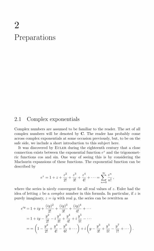
Complex numbers are assumed to be familiar to the reader. The set of allcomplex numbers will be denoted by C. The reader has probably comeacross complex exponentials at some occasion previously, but, to be on thesafe side, we include a short introduction to this subject here.
It was discovered by Euler during the eighteenth century that a closeconnection exists between the exponential function ez and the trigonomet-ric functions cos and sin. One way of seeing this is by considering theMaclaurin expansions of these functions. The exponential function can bedescribed by
ez = 1 + z +z2
2!+z3
3!+z4
4!+ · · · =
∞∑n=0
zn
n!,
where the series is nicely convergent for all real values of z. Euler had theidea of letting z be a complex number in this formula. In particular, if z ispurely imaginary, z = iy with real y, the series can be rewritten as
eiy = 1 + iy +(iy)2
2!+
(iy)3
3!+
(iy)4
4!+ · · ·
= 1 + iy − y2
2!− i
y3
3!+y4
4!+ i
y5
5!− · · ·
= =(
1 − y2
2!+y4
4!− y6
6!+ · · ·
)+ i
(y − y3
3!+y5
5!− y7
7!+ · · ·
).

16 2. Preparations
In the brackets we recognize the well-known expansions of cos and sin:
cos y = 1 − y2
2!+y4
4!− y6
6!+ · · · ,
sin y = y − y3
3!+y5
5!− y7
7!+ · · · .
Accordingly, we defineeiy = cos y + i sin y. (2.1)
This is one of the so-called Eulerian formulae. The somewhat adventurousmotivation through our manipulation of a series can be completely justified,which is best done in the context of complex analysis. For this book we shallbe satisfied that the formula is true and can be used.
What is more, one can define exponentials with general complex argu-ments:
ex+iy = exeiy = ex(cos y + i sin y) if x and y are real.
The function thus obtained obeys most of the well-known rules for the realexponential function. Notably, we have these rules:
ezew = ez+w,1ez
= e−z,ez
ew= ez−w.
It is also true that ez = 0 for all z, but it need no longer be true thatez > 0.
Example 2.1. eiπ = cosπ + i sinπ = −1 + i · 0 = −1. Also, eniπ = (−1)n
if n is an integer (positive, negative, or zero). Furthermore, eiπ/2 = i isnot even real. Indeed, the range of the function ez for z ∈ C contains allcomplex numbers except 0. Example 2.2. The modulus of a complex number z = x + iy is definedas |z| =
√zz =
√x2 + y2. As a consequence,
|ez| = |ex+iy| = |ex · eiy| = ex| cos y + i sin y| = ex
√cos2 y + sin2 y = ex.
In particular, if z = iy is a purely imaginary number, then |ez| = |eiy| = 1.
Example 2.3. Let us start from the formula eixeiy = ei(x+y) and rewriteboth sides of this, using (2.1). On the one hand we have
eixeiy = (cosx+ i sinx)(cos y + i sin y)= cosx cos y − sinx sin y + i(cosx sin y + sinx cos y),
and on the other hand,
ei(x+y) = cos(x+ y) + i sin(x+ y).

2.2 Complex-valued functions of a real variable 17
If we identify the real and imaginary parts of the trigonometric expressions,we see that
cos(x+ y) = cosx cos y − sinx sin y, sin(x+ y) = cosx sin y + sinx cos y.
Thus the addition theorems for cos and sin are contained in a well-knownexponential law!
By changing the sign of y in (2.1) and then manipulating the formulaeobtained, we find the following set of equations:
eiy = cos y + i sin y
e−iy = cos y − i sin y
cos y =eiy + e−iy
2
sin y =eiy − e−iy
2i
These are the “complete” set of Euler’s formulae. They show how one canpass back and forth between trigonometric expressions and exponentials.
Particularly in Chapters 4 and 7, but also in other chapters, we shalluse the exponential expressions quite a lot. For this reason, the readershould become adept at using them by doing the exercises at the end ofthis section. If these things are quite new, the reader is also advised to findmore exercises in textbooks where complex numbers are treated.
Exercises2.1 Compute the numbers eiπ/2, e−iπ/4, e5πi/6, eln 2−iπ/6.
2.2 Prove that the function f(z) = ez has period 2πi, i.e., that f(z+2πi) = f(z)for all z.
2.3 Find a formula for cos 3t, expressed in cos t, by manipulating the identitye3it =
(eit)3
.
2.4 Prove the formula sin3 t = 34 sin t− 1
4 sin 3t.
2.5 Show that if |ez| = 1, then z is purely imaginary.
2.6 Prove the de Moivre formula:
(cos t+ i sin t)n = cosnt+ i sinnt, n integer.
2.2 Complex-valued functions of a real variable
In order to perform calculus on complex-valued functions, we should definelimits of such objects. As long as the domain of definition lies on the realaxis, this is quite simple and straightforward. One can use similar formu-lations as in the all-real case, but now modulus signs stand for moduli ofcomplex numbers. For example: if we state that
limt→∞ f(t) = A,

18 2. Preparations
then we are asserting the following: for every positive number ε, there existsa number R such that as soon as t > R we are assured that |f(t) −A| < ε.
If we split f(t) into real and imaginary parts,
f(t) = u(t) + iv(t), u(t) and v(t) real,
the following inequalities hold:
|u(t)| ≤ |f(t)|, |v(t)| ≤ |f(t)|; |f(t)| ≤ |u(t)| + |v(t)|. (2.2)
This should make it rather clear that convergence in a complex-valuedsetting is equivalent to the simultaneous convergence of real and imaginaryparts. Indeed, if the latter are both small, then the complex expressionis small; and if the complex expression is small, then both its real andimaginary parts must be small. In practice this means that passing toa limit can be done in the real and imaginary parts, which reduces thecomplex-valued situation to the real-valued case.
Thus, if we want to define the derivative of a complex-valued functionf(t) = u(t) + iv(t), we can go about it in two ways. Either we define
f ′(t) = limh→0
f(t+ h) − f(t)h
,
which stands for an ε-δ notion involving complex numbers, or we can justsay that
f ′(t) = u′(t) + iv′(t). (2.3)
These definitions are indeed equivalent. The derivative of a complex-valuedfunction of a real variable t exists if and only if the real and imaginary partsof f both have derivatives, and in this case we also have the formula (2.3).The following example shows the most frequent case of this, at least in thisbook.
Example 2.4. If f(t) = ect with a complex coefficient c = α+ iβ, we canfind the derivative, according to (2.3), like this:
f ′(t) =d
dt
(eαt(cosβt+ i sinβt)
)=
d
dt
(eαt cosβt
)+ i
d
dt
(eαt sinβt
)= αeαt cosβt− eαtβ sinβt+ i
(αeαt sinβt+ eαtβ cosβt
)= eαt(α+ iβ)(cosβt+ i sinβt) = cect.
Similarly, integration can be defined by splitting into real and imaginary
parts. If I is an interval, bounded or unbounded,∫I
f(t) dt =∫
I
(u(t) + iv(t)) dt =∫
I
u(t) dt+ i
∫I
v(t) dt.
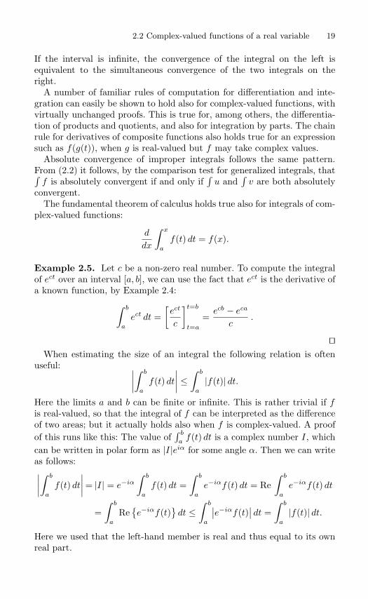
2.2 Complex-valued functions of a real variable 19
If the interval is infinite, the convergence of the integral on the left isequivalent to the simultaneous convergence of the two integrals on theright.
A number of familiar rules of computation for differentiation and inte-gration can easily be shown to hold also for complex-valued functions, withvirtually unchanged proofs. This is true for, among others, the differentia-tion of products and quotients, and also for integration by parts. The chainrule for derivatives of composite functions also holds true for an expressionsuch as f(g(t)), when g is real-valued but f may take complex values.
Absolute convergence of improper integrals follows the same pattern.From (2.2) it follows, by the comparison test for generalized integrals, that∫f is absolutely convergent if and only if
∫u and
∫v are both absolutely
convergent.The fundamental theorem of calculus holds true also for integrals of com-
plex-valued functions:
d
dx
∫ x
a
f(t) dt = f(x).
Example 2.5. Let c be a non-zero real number. To compute the integralof ect over an interval [a, b], we can use the fact that ect is the derivative ofa known function, by Example 2.4:∫ b
a
ect dt =[ect
c
]t=b
t=a
=ecb − eca
c.
When estimating the size of an integral the following relation is often
useful: ∣∣∣∣∫ b
a
f(t) dt∣∣∣∣ ≤
∫ b
a
|f(t)| dt.
Here the limits a and b can be finite or infinite. This is rather trivial if fis real-valued, so that the integral of f can be interpreted as the differenceof two areas; but it actually holds also when f is complex-valued. A proofof this runs like this: The value of
∫ b
af(t) dt is a complex number I, which
can be written in polar form as |I|eiα for some angle α. Then we can writeas follows:∣∣∣∣∫ b
a
f(t) dt∣∣∣∣= |I| = e−iα
∫ b
a
f(t) dt =∫ b
a
e−iαf(t) dt = Re∫ b
a
e−iαf(t) dt
=∫ b
a
Ree−iαf(t)
dt ≤
∫ b
a
∣∣e−iαf(t)∣∣ dt =
∫ b
a
|f(t)| dt.
Here we used that the left-hand member is real and thus equal to its ownreal part.
20 2. Preparations
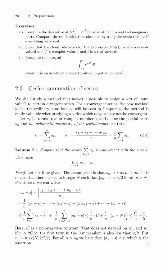
Exercises2.7 Compute the derivative of f(t) = eit2 by separating into real and imaginary
parts. Compare the result with that obtained by using the chain rule, as ifeverything were real.
2.8 Show that the chain rule holds for the expression f(g(t)), where g is real-valued and f is complex-valued, and t is a real variable.
2.9 Compute the integral ∫ π
−π
eint dt,
where n is an arbitrary integer (positive, negative, or zero).
2.3 Cesaro summation of series
We shall study a method that makes it possible to assign a sort of “sumvalue” to certain divergent series. For a convergent series, the new methodyields the ordinary sum; but, as will be seen in Chapter 4, the method isreally valuable when studying a series which may or may not be convergent.
Let ak be terms (real or complex numbers), and define the partial sumssn and the arithmetic means σn of the partial sums like this:
sn =n∑
k=1
ak, σn =s1 + s2 + · · · + sn
n=
1n
n∑k=1
sk. (2.4)
Lemma 2.1 Suppose that the series∞∑
k=1ak is convergent with the sum s.
Then alsolim
n→∞σn = s.
Proof. Let ε > 0 be given. The assumption is that sn → s as n → ∞. Thismeans that there exists an integer N such that |sn −s| < ε/2 for all n > N .For these n we can write
|σn − s| =∣∣∣∣s1 + s2 + · · · + sn − ns
n
∣∣∣∣=
1n
∣∣(s1 − s) + · · · + (sN − s) + (sN+1 − s) + · · · + (sn − s)∣∣
≤ 1n
N∑k=1
|sk − s| +1n
n∑k=N+1
|sk − s| ≤ 1n
· C +1n
· (n−N)ε
2≤ C
n+ε
2.
Here, C is a non-negative constant (that does not depend on n), and so,if n > 2C/ε, the first term in the last member is also less than ε/2. Putn0 = max(N, 2C/ε). For all n > n0 we have then |σn − s| < ε, which is theassertion.

2.3 Cesaro summation of series 21
Definition 2.1 Let sn and σn be defined as in (2.4). We say that theseries
∑∞k=1 ak is summable according to Cesaro or Cesaro summable
or summable (C, 1) to the value, or “sum”, s, if limn→∞σn = s.
We write ∞∑k=1
ak = s (C, 1).
The lemma above states that if a series is convergent in the usual sense,then it is also summable (C, 1), and the Cesaro sum coincides with theordinary sum.
Example 2.6. Let ak = (−1)k−1, k = 1, 2, 3, . . ., which means that wehave the series 1 − 1 + 1 − 1 + 1 − 1 + · · ·. Then sn = 0 if n is even andsn = 1 if n is odd. The means σn are
σn =12
if n is even, σn =12 (n+ 1)
n=n+ 12n
if n is odd.
Thus we have σn → 12 as n → ∞. This divergent series is indeed summable
(C, 1) with sum 12 .
The reason for the notation (C, 1) is that it is possible to iterate theprocess. If the σn do not converge, we can form the means τn = (σ1 + · · ·+σn)/n. If the τn converge to a number s one says that the original series is(C, 2)-summable to s, and so on.
These methods can be efficient if the terms in the series have differentsigns or are complex numbers. A positive divergent series cannot be summedto anything but +∞, no matter how many means you try.
Exercises
2.10 Study the series 1 + 0 − 1 + 1 + 0 − 1 + 1 + 0 − · · ·, i.e., the series∑∞
k=1 ak,where a3k+1 = 1, a3k+2 = 0 and a3k+3 = −1. Compute the Cesaro meansσn and show that the series has the Cesaro sum 2
3 .
2.11 The results of Example 2.6 and the previous exercise can be generalized asfollows. Assume that the sequence of partial sums sn is periodic, i.e., thatthere is a positive integer p such that sn+p = sn for all n. Then the seriesis summable (C, 1) to the sum σ = (s1 + s2 + · · · + sp)/p. Prove this!
2.12 Show that if∑
ak has a finite (C, 1) value, then
limn→∞
sn
n= 0.
What can be said about limk→∞
ak/k ?
2.13 Prove that if ak ≥ 0 and∑
ak is (C, 1)-summable, then the series is con-vergent in the usual sense. (Assume the contrary – what does that entailfor a positive series?)

22 2. Preparations
2.14 Show that the series∑∞
k=1(−1)k k is not summable (C, 1). Also show thatit is summable (C, 2). Show that the (C, 2) sum is equal to − 1
4 .
2.15 Show that, if x = n · 2π (n ∈ Z),
12 +
∞∑k=1
cos kx = 0 (C, 1).
2.16 Prove that∞∑
n=0
zn =1
1 − z(C, 1) for |z| ≤ 1, z = 1.
2.4 Positive summation kernels
In this section we prove a theorem that is useful in many situations forrecovering the values of a function from various kinds of transforms. Themain idea is summarized in the following formulation.
Theorem 2.1 Let I = (−a, a) be an interval (finite or infinite). Supposethat Kn∞
n=1 is a sequence of real-valued, Riemann-integrable functionsdefined on I, with the following properties:
(1) Kn(s) ≥ 0.
(2)∫ a
−a
Kn(s) ds = 1.
(3) If δ > 0, then limn→∞
∫δ<|s|<a
Kn(s) ds = 0.
If f : I → C is integrable and bounded on I and continuous for s = 0, wethen have
limn→∞
∫ a
−a
Kn(s) f(s) ds = f(0).
Proof. Let ε be a positive number. Since f is continous at the origin thereexists a number δ > 0 such that
|s| ≤ δ ⇒ |f(s) − f(0)| < ε.
Furthermore, f is bounded on I, i.e., there exists a number M such that|f(s)| ≤ M for all s. Because of the property 2 we have
∆ :=∫ a
−a
Kn(s) f(s) ds− f(0) =∫ a
−a
Kn(s) f(s) ds− f(0)∫ a
−a
Kn(s) ds
=∫ a
−a
Kn(s)(f(s) − f(0)
)ds.
2.4 Positive summation kernels 23
We want to prove that ∆ → 0 as n → ∞. Let us estimate the absolutevalue of ∆, assuming that |s| ≤ δ:
|∆| =∣∣∣∣∣∣
a∫−a
Kn(s)(f(s) − f(0)
)ds
∣∣∣∣∣∣ ≤a∫
−a
Kn(s) |f(s) − f(0)| ds
=
δ∫−δ
Kn(s) |f(s) − f(0)| ds+∫
δ<|s|<a
Kn(s) |f(s) − f(0)| ds
≤ ε
δ∫−δ
Kn(s) ds+∫
δ<|s|<a
Kn(s) 2M ds ≤ ε+ 2M∫
δ<|s|<a
Kn(s) ds.
The last integral tends to zero, by the assumptions, and so the second termof the last member is also less than ε if n is large enough. This means thatfor large n we have |∆| < 2ε, which proves the theorem.
A sequence Kn∞n=1 having the properties 1–3 is called a positive sum-
mation kernel. We illustrate with a few simple examples.
Example 2.7. Define Kn : R → R by
Kn(s) =n, |s| < 1/(2n),0, |s| > 1/(2n)
(see Figure 2.1a). It is obvious that the conditions 1–3 are fullfilled. Seealso Exercise 2.17. Example 2.8. Let ϕ(s) = e−s2/2/
√2π, the density function of the normal
probability distribution (Figure 2.1b). Define Kn(s) = nϕ(ns). Then Knis a positive summation kernel on R (check it!). Example 2.9. The preceding example can be generalized in the followingway: Let ψ : R → R be some function satisfying ψ(s) ≥ 0 and
∫R ψ(s) ds =
1. Putting Kn(s) = nψ(ns), we have a positive summation kernel. The examples should help the reader to understand what is going on: a
positive summation kernel creates a weighted mean value of the function f ,with the weight being successively concentrated towards the point s = 0.If f is continuous at that point, the limit will yield precisely the value of fat s = 0.
A corollary of Theorem 2.1 is the following, where we move the concen-tration of mass to some other point than the origin:
Corollary 2.1 If Kn∞n=1 is a positive summation kernel on the interval
I, s0 is an interior point of I, and f is continuous at s = s0, then
limn→∞
∫I
Kn(s) f(s0 − s) ds = f(s0).

24 2. Preparations
12n− 1
2n
n
s
(a)
sK1
K3
(b)
FIGURE 2.1.
The proof is left as an exercise (do the change of variable s0 − s = u).
Remark. The choice of the interval I is often rather unimportant. It is also easyto see that the condition 2 can be weakened, e.g., it suffices that the integrals ofKn over the interval tend to 1 as n → ∞. In consequence, kernels on all of R canalso be used on any subinterval R having the origin in its interior.
Remark. The reader who is familiar with the notion of uniform continuity , canappreciate a sharper formulation of the corollary: if f is continuous on a compactinterval K, the functions
Fn(t) =∫
I
Kn(s)f(t− s) ds
will converge to f(t) uniformly on K. The proof is practically unchanged, withthe only addition that the number δ occuring in the proof of Theorem 2.1 can bechosen so that it can be used simultaneously for all values of t that are involved.
Exercises2.17 Prove directly, without using the theorem, that if Kn is as in Example 2.7
and f is continuous at the origin, then limn→∞
∫RKn(s)f(s) ds = f(0).
2.18 Prove that the “roof functions” gn, defined by gn(t) = n − n2t for 0 ≤t ≤ 1/n, gn(t) = 0 for t > 1/n and gn(−t) = gn(t), make up a positivesummation kernel. Draw pictures!
2.19 (a) Show that Kn(t) = 12ne
−n|t| describes a positive summation kernel.(b) Suppose that f is bounded and piecewise continuous on R, andlimt0
f(t) = 1, limt0
f(t) = 3. Show that
limn→∞
n
2
∫R
e−n|t| f(t) dt = 2.

2.5 The Riemann–Lebesgue lemma 25
2.20 Show that if f is bounded on R and has a derivative f ′ that is also boundedon R and continuous at the origin, then
limn→∞
n3
√2π
∫R
s e−n2s2/2 f(s) ds = f ′(0).
2.21 Let ϕ be defined by ϕ(x) = 1516 (x2 −1)2 for |x| < 1 and ϕ(x) = 0 otherwise.
Let f be a function with a continuous derivative. Find the limit
limn→∞
∫ 1
−1
n2ϕ′(nx) f(x) dx.
2.5 The Riemann–Lebesgue lemma
The following theorem plays a central role in Fourier Analysis. It takesits name from the fact that it holds even for functions that are integrableaccording to the definition of Lebesgue. We prove it for functions that areabsolutely integrable in the Riemann sense. First, let us very briefly recallwhat this means.
A bounded function f on a finite interval [a, b] is integrable if it can beapproximated by Riemann sums from above and below in such a way thatthe difference of the integrals of these sums can be made as small as wewish. This definition is then extended to unbounded functions and infiniteintervals by taking limits; these cases are often called improper integrals. IfI is any interval and f is a function on I such that the (possibly improper)integral ∫
I
|f(u)| du
has a finite value, then f is said to be absolutely integrable on I.
Theorem 2.2 (Riemann–Lebesgue lemma) Let f be absolutely inte-grable in the Riemann sense on a finite or infinite interval I. Then
limλ→∞
∫I
f(u) sinλu du = 0.
Proof. We do it in four steps. First, assume that the interval is compact,I = [a, b], and that f is constant and equal to 1 on the entire interval. Then∫ b
a
f(u) sinλu du =∫ b
a
sinλu du =[−cosλu
λ
]u=b
u=a
=1λ
(cosλa− cosλb),
which gives ∣∣∣∣∣∫ b
a
f(u) sinλu du
∣∣∣∣∣ ≤ 2λ
−→ 0 as λ → ∞.
26 2. Preparations
The assertion is thus true for this f .Now assume that f is piecewise constant, which means that I (still as-
sumed to be compact) is subdivided into a finite number of subintervalsIk = (ak−1, ak), k = 1, 2, . . . , N (a0 = a, aN = b), and that f(u) has acertain constant value ck for u ∈ Ik. This means that we can write
f(u) =N∑
k=1
ck gk(u),
where gk(u) = 1 on Ik and gk(u) = 0 outside of Ik. We get
∫ b
a
f(u) sinλu du =N∑
k=1
∫ b
a
ck gk(u) sinλu du =N∑
k=1
ck
∫ ak
ak−1
sinλu du.
This is a sum of finitely many terms, and by the preceding case each ofthese terms tends to zero as λ → ∞. Thus the assertion is true also for thisf .
Let now f be an arbitrary function that is Riemann integrable on I =[a, b]. Let ε be an arbitrary positive number. By the definition of the Rie-mann integral, there exists a piecewise constant function g such that∫ b
a
|f(u) − g(u)| du < ε
2.
(Let g be a function whose integral is a Riemann sum of f .) Then,∣∣∣∣∣∫ b
a
f(u) sinλu du
∣∣∣∣∣=∣∣∣∣∣∫ b
a
(f(u) − g(u)) sinλu du+∫ b
a
g(u) sinλu du
∣∣∣∣∣≤∫ b
a
|f(u) − g(u)|| sinλu| du+
∣∣∣∣∣∫ b
a
g(u) sinλu du
∣∣∣∣∣≤∫ b
a
|f(u) − g(u)| du+
∣∣∣∣∣∫ b
a
g(u) sinλu du
∣∣∣∣∣ .The last integral tends to zero as λ → ∞, by the preceding case. Thus thereis a value λ0 such that this integral is less that ε/2 for all λ > λ0. For theseλ, the left-hand member is thus less than ε, which proves the assertion.
Finally, we no longer require that I is compact. Let ε > 0 be prescribed.Since f is absolutely integrable, there is a compact subinterval J ⊂ I suchthat
∫I\J
|f(u)| du < ε. We can write∣∣∣∣∫I
f(u) sinλu du∣∣∣∣ ≤
∣∣∣∣∫J
f(u) sinλu du∣∣∣∣+ ∫
I\J
|f(u)| du,

2.6 *Some simple distributions 27
where the first term tends to zero by the preceding case, and thus it is lessthan ε if λ is large enough; the second term is always less than ε. Thiscompletes the proof.
The intuitive content of the theorem is not hard to understand: For largevalues of |λ|, the integrated function f(u) sinλu is an amplitude-modulatedsine function with a high frequency; its mean value over a fixed intervalshould reasonably approach zero as the frequency increases. Of course,the factor sinλu in the integral can be replaced by cosλu or the complexfunction eiλu, with the same result. And, of course, we can just as well letλ tend to −∞.
2.6 *Some simple distributions
In this section, we introduce, in an informal way, a sort of generalization ofthe notion of a function. (A more coherent and systematic way of definingthese objects is given in Chapter 8.) As a motivation for this generalization,we begin with a few “examples.”
Example 2.10. In Sec. 1.3 (on the wave equation) we saw difficulties in theusual requirement that solutions of a differential equation of order n shallactually have (maybe even continuous) derivatives of order n. Quite naturalsolutions are disqualified for reasons that seem more of a “bureaucratic”nature than physically motivated. This indicates that it would be a goodthing to widen the notion of differentiability in one way or another.
Example 2.11. Ever since the days of Newton, physicists have beendealing with situations where some physical entity assumes a very largemagnitude during a very short period of time; often this is idealized sothat the value is infinite at one point in time. A simple example is an elas-tic collision of two bodies, where the forces are thought of as infinite atthe moment of impact. Nevertheless, a finite and well-defined amount ofimpulse is transferred in the collision. How is this to be treated mathemat-ically?
Example 2.12. A situation that is mathematically analogous to theprevious one is found in the theory of electricity. An electron is considered(at least in classical quantum theory) to be a point charge. This means thatthere is a certain finite amount of electric charge localized at one point inspace. The charge density is infinite at this point, but the charge itself hasan exact, finite value. What mathematical object describes this?
Example 2.13. In Sec. 2.4 we studied positive summation kernels. Theseconsisted of sequences of nonnegative functions with integral equal to 1,that concentrate toward a fixed point as a parameter, say, N , tends to

28 2. Preparations
infinity, for example. Can we invent a mathematical object that can beinterpreted as the limit of such a sequence?
The problems in Examples 2.11 and 2.12 above have been addressed bymany physicists ever since the later years of the nineteenth century byusing the following trick. Let us assume that the independent variable is t.Introduce a “function” δ(t) with the following properties:
(1) δ(t) ≥ 0 for − ∞ < t < ∞,
(2) δ(t) = 0 for t = 0,
(3)∫ ∞
−∞δ(t) dt = 1.
Regrettably, there is no ordinary real-(or complex)-valued function thatsatisfies these conditions. Condition 2 irrevocably implies that the integralin condition 3 must be zero. Nevertheless, using formal calculations involv-ing the “function” δ, it was possible to arrive at results that were bothphysically meaningful and “correct.” A name that is commonly associatedwith this is P. Dirac, but he was not the only person (nor even the firstone) to reason in this way. He has, however, given his name to the objectδ: it is often called the Dirac delta function (or the Dirac measure, or theDirac distribution).
One way of making legitimate the formal δ calculus is to follow an ideathat is indicated in Example 2.13. If δ occurs in a formula, it is at firstreplaced by a positive summation kernel KN ; upon this we then do ourcalculations, and finally we pass to the limit. In a certain sense (which willbe made precise in Chapter 8), it is true that δ = lim
N→∞KN .
In this section, and in certain star-marked sections in the following chap-ters, we shall accept the delta function and some of its relatives in an intu-itive way. Thus, δ(t) stands for an object that acts on a continuous functionϕ according to the formula∫
δ(t)ϕ(t) dt = ϕ(0),
where the integral is taken over some interval that contains the origin inits interior. We also introduce the translates δa, which can be describedby either δa(t) = δ(t − a) or
∫δa(t)ϕ(t) dt = ϕ(a). It is essential that the
point a, where the “pulse” appears, is located in the interior of the intervalof integration. If the point coincides with an endpoint of the interval, theintegral is not considered to be well-defined.
Example 2.14. The Laplace transform of a function f is defined to beanother function f , given by
f(s) =∫ ∞
0f(t)e−st dt

2.6 *Some simple distributions 29
for all s such that the integral is convergent (see Chapter 3). The Laplacetransform of δ cannot be defined in this way. We can, however, modify thedefinition so as to include the origin. It is indeed customary to write
f(s) =∫ ∞
0−f(t)e−st dt = lim
k0
∫ ∞
k
f(t)e−st dt.
With this definition one finds that δ(s) = 1 for all s. Similarly, δa(s) = e−as,if a > 0.
The Heaviside function, or unit step function, H is defined by
H(t) =
0 for t < 0,1 for t > 0.
The value of H(0) is mostly left undefined, because it is normally of noimportance. The Heaviside function is useful in many contexts. One ofthese is when we are dealing with functions that are given by differentformulae in different intervals.
If a < b, the expression H(t−a)−H(t−b) is equal to 1 for a < t < b andequal to 0 outside the interval [a, b]. It might be called a “window” thatlights up the interval (a, b) (we do not in these situations care much aboutwhether an interval is open or closed). For unbounded intervals we can alsofind “windows”: the function H(t − a) lights up the interval (a,∞), andthe expression 1 −H(t− b) the interval (−∞, b).
Example 2.15. Consider the function f : R → R that is given by
f(t) =
1 − t2 for t < −2,t+ 2 for − 2 < t < 1,1 − t for t > 1.
This can now be compressed into one formula:
f(t)= (1 − t2)(1 −H(t+ 2)) + (t+ 2)(H(t+ 2)−H(t− 1)) + (1 − t)H(t− 1)= (1 − t2) + (−1 + t2 + t+ 2)H(t+ 2) + (−t− 2 + 1 − t)H(t− 1)= 1 − t2 + (t2 + t+ 1)H(t+ 2) − (2t+ 1)H(t− 1).
Heaviside’s function is connected with the δ function via the formula
H(t) =∫ t
−∞δ(u) du.
A very bold differentiation of this formula would give the result
H ′(t) = δ(t). (2.5)

30 2. Preparations
Since H is constant on the intervals ]−∞, 0[ and ]0,∞[, and δ(t) is consid-ered to be zero on these intervals, the formula (2.5) is reasonable for t = 0.What is new is that the “derivative” of the jump discontinuity of H shouldbe considered to be the “pulse” of δ. In fact, this assertion can be given acompletely coherent background; this will be done in Chapter 8.
If ϕ is a function in the class C1, i.e., it has a continuous derivative, andif in addition ϕ is zero outside some finite interval, the following calculationis clear:∫ ∞
−∞ϕ′(t)H(t) dt =
∫ ∞
0ϕ′(t) dt =
[ϕ(t)
]∞t=0 = 0 − ϕ(0) = −ϕ(0).
The same result can also be obtained by the following formal integrationby parts: ∫ ∞
−∞ϕ′(t)H(t) dt=
[ϕ(t)H(t)
]∞
−∞−∫ ∞
−∞ϕ(t)H ′(t) dt
= (0 − 0) −∫ ∞
−∞ϕ(t)δ(t) dt = −ϕ(0).
This is characteristic of the way in which these generalized functions can betreated: if they occur in an integral together with an “ordinary” functionof sufficient regularity, this integral can be treated formally, and the resultswill be true facts.
One can go further and introduce derivatives of the δ functions. Whatwould be, for example, the first derivative of δ = δ0 ? One way of finding outis by operating formally as in the preceding situation. Let ϕ be a functionin C1, and let it be understood that all integrals are taken over an intervalthat contains 0 in its interior. Since δ(t) = 0 if t = 0, it is reasonable thatalso δ′(t) = 0 for t = 0. Integration by parts gives∫ b
a
δ′(t)ϕ(t) dt =[δ(t)ϕ(t)
]b
a
−∫ b
a
δ(t)ϕ′(t) dt = (0 − 0) − ϕ′(0) = −ϕ′(0).
If δ itself serves to pick out the value of a function at the origin, thederivative of δ can thus be used to find the value at the same place ofthe derivative of a function.
Another way of seeing δ′ is to consider δ to be the limit of a differentiablepositive summation kernel, and taking the derivative of the kernel. Anexample is actually given in Exercise 2.20. As in Example 2.8 on page 23,we study the summation kernel
Kn(t) =n√2π
e−n2t2/2,
(which consists in rescaling the normal probability density function). Thederivatives are
Kn′(t) = − n3t√
2πe−n2t2/2.

2.6 *Some simple distributions 31
t
K1
K2
FIGURE 2.2.
t
q
−q
1/q
FIGURE 2.3.
These are illustrated in Figure 2.2. The fact that they approach −δ′(t) isproved by integration by parts (which is what Exercise 2.20 is all about).
In the theory of electricity, there occurs a phenomenon known as anelectric dipole. This consists of two equal but opposite charges ±q at asmall distance from each other (see Figure 2.3). If the distance is madesmaller and charges increase in proportion to the inverse of the distance,the “limit object” is an idealized dipole. A mathematical model of thisobject consists of δ′, just as a a point charge can be represented by δ.
Higher derivatives of δ can also be defined. Using integration by partsone finds that the nth derivative δ(n) should act according to the formula∫
δ(n)(t)ϕ(t) dt = (−1)n ϕ(n)(0),
provided the function ϕ has an nth derivative that is continuous at theorigin.

32 2. Preparations
Exercises2.22 Compute the following integrals (taken over the entire real axis if nothing
else is indicated):(a)
∫(t2 + 3t)(δ(t) − δ(t+ 2)) dt (b)
∫∞0e−stδ′(t− 1) dt
(c)∫e2tδ′(t) dt (d)
∫∞0− δ
(n)(t) e−st dt
2.23 What should be meant by δ(2t), expressed using δ(t) ? Investigate this bymanipulating
∫ϕ(t)δ(2t) dt in a suitable way. Generalize to δ(at), a = 0.
(The cases a > 0 and a < 0 should be considered separately.)
2.24 Rewrite, using Heaviside windows, the expressions f1(t) = t|t+ 1|, f2(t) =e−|t|, f3(t) = sgn t = t/|t| (t = 0), f4(t) = A if t < a, = B if t > a.
2.7 *Computing with δ
We shall now show how one can solve certain problems involving the δdistribution and its derivatives.
The ordinary rules for computing with derivatives will still hold true.(We cannot really prove this at the present stage.) For example, the rulefor differentiating a product is valid: (fg)′ = f ′g + fg′.
Example 2.16. If χ is a function that is continuous at a, what should bemeant by the product χ(t)δa(t) ? Since δa(t) is “zero” except for at t = a, itcan be expected that the values of χ(t) for t = a should not really matter.And we can write as follows:∫ (
χ(t)δa(t))ϕ(t) dt =
∫δa(t)
(χ(t)ϕ(t)
)dt = χ(a)ϕ(a).
There is no way to distinguish χ(t)δa(t) from χ(a)δa(t). Thus we have asimplification rule: the product of a delta and a continuous function is equalto a scalar multiple of the delta, with coefficient equal to the value of thefunction at the point where the pulse sits:
χ(t)δa(t) = χ(a)δa(t). (2.6)
If we encounter derivatives of δ, the matter is more complicated. Whathappens is this: start from (2.6) and differentiate:
χ′(t)δa(t) + χ(t)δ′a(t) = χ(a)δ′
a(t).
In the first term we can replace χ′(t) by χ′(a) and then move this term tothe other side. We get
χ(t)δ′a(t) = χ(a)δ′
a(t) − χ′(a)δa(t).
(On second thought, it should not be surprising that the product of afunction and a δ′ somehow takes into account the value of the derivativeof the function as well.)

2.7 *Computing with δ 33
What happens when the second derivative is multiplied by a function isleft to the reader to find out (in Exercise 2.25). Example 2.17. Find the first two derivatives of f(t) = |t|.Solution. Rewrite the function without modulus signs, using Heaviside win-dows:
f(t) = |t| = −t(1 −H(t)) + tH(t) = 2tH(t) − t.
Differentiation then gives
f ′(t) = 2H(t) + 2tδ(t) − 1 = 2H(t) − 1.
In the last step we used the formula (2.6). In plain language, the derivativeof |t| is plus one for positive t and minus one for negative t, just as weknow from elementary calculus; at the origin, the value of the derivative isundecided. We proceed to the second derivative:
f ′′(t) = 2δ(t) − 0 = 2δ(t).
This formula reflects the fact that f ′ has derivative zero everywhere outsidethe origin; whereas at the origin, the delta term indicates that f ′ has apositive jump of two units. This is characteristic of the derivative of afunction with jumps. Example 2.18. Another example of the same type, though more compli-cated. The function f(x) = |x2 − 1| can be rewritten as
f(x) = (x2 − 1)H(x− 1) + (1 − x2)(H(x+ 1) −H(x− 1))+(x2 − 1)(1 −H(x+ 1))
= (x2 − 1)(2H(x− 1) − 2H(x+ 1) + 1
).
This formula can be differentiated, using the rule for differentiating a prod-uct:
f ′(x) = 2x(2H(x− 1) − 2H(x+ 1) + 1
)+ (x2 − 1)
(2δ(x− 1) − 2δ(x+ 1)
)= 2x
(2H(x− 1) − 2H(x+ 1) + 1
).
In the last step, we used (2.6). One more differentiation gives
f ′′(x) = 2(2H(x− 1) − 2H(x+ 1) + 1
)+ 2x
(2δ(x− 1) − 2δ(x+ 1)
)= 2
(2H(x− 1) − 2H(x+ 1) + 1
)+ 4δ(x− 1) + 4δ(x+ 1).
The first term contains the classical second derivative of |x2 − 1|, whichexists for x = ±1; the two δ terms demonstrate that f ′ has upward jumpsof size 4 for x = ±1. The reader should draw pictures of f , f ′, and f ′′.
In the two last examples, the first derivative at the “corners” of f isconsidered to be undecided. The classical point of view is to say that f does

34 2. Preparations
not have a derivative at such a point; when working with distributions, thederivative is thought of as more of a global notion, that always exists, butmay lack a precise value at certain points.
Example 2.19. Solve the differential equation y′ +2y = δ(t− 1) for t > 0with the initial value y(0) = 1.
Solution. The method of integrating factor can be used. An integratingfactor is e2t:
e2ty′ + 2e2ty = e2tδ(t− 1) ⇐⇒ d
dt
(e2t y
)= e2δ(t− 1).
In rewriting the right-hand side we used (2.6). Now we can integrate:
e2t y = e2H(t− 1) + C,
where C is a constant. To satisfy the initial condition, we must take C = 1.Thus the solution is
y = e2−2tH(t− 1) + e−2t, t > 0.
(The reader is recommended to check the solution by differentiation andsubstitution into the original equation.) Example 2.20. Find all solutions of the differential equation y′′ +4y = δ.
Solution. The classical method for this sort of problem amounts to firstfinding the general solution of the corresponding homogeneous equation,which is yH = C1 cos 2t + C2 sin 2t, where C1 and C2 are arbitrary con-stants. Then we should find some particular solution of the inhomogeneousequation. What kind of expression yP could possibly, after differentiationand substitution into the left-hand side of the equation, yield the resultδ? Apparently, something drastic happens at t = 0. Since δ(t) = 0 fort < 0, the equation can be said to be homogeneous during this periodof time. Let us then guess that there is a particular solution of the formyP (t) = u(t)H(t), where u(t) is to be determined. Differentiation gives
y′P (t) = u′(t)H(t) + u(t)H ′(t) = u′(t)H(t) + u(0)δ(t),y′′
P (t) = u′′(t)H(t)+u′(t)H ′(t)+u(0)δ′(t)= u′′(t)H(t)+u′(0)δ(t)+u(0)δ′(t).
Substitution into the equation gives(u′′(t)H(t) + u′(0)δ(t) + u(0)δ′(t)
)+ 4u(t)H(t) = δ(t)
or (u′′(t) + 4u(t)
)H(t) + u′(0)δ(t) + u(0)δ′(t) = δ(t).

2.7 *Computing with δ 35
The function u should be chosen so that u′′ + 4u = 0, u′(0) = 1 andu(0) = 0. This means that u(t) = a cos 2t+b sin 2t, where 0 = u(0) = a and1 = u′(0) = 2b. Thus, u = 1
2 sin 2t, and yP = 12 sin 2tH(t). The solutions of
the problem are thus
y = C1 cos 2t+ (C2 + 12H(t)) sin 2t.
Again, the reader is recommended to check the solution. Example 2.21. In Sec. 1.3, on the wave equation, the final example turnedout to have a solution that was not really a differentiable function. Nowwe can put this right, by allowing the generalized derivatives introduced inthis section. The solution involved the function ϕ, defined by
ϕ(s) = 12 s− 1
2 C for s > 0, ϕ(s) = − 12 s− 1
2 C for s < 0.
We can rewrite this definition, using Heaviside windows:
ϕ(s) = (− 12 s− 1
2 C)(1 −H(s)) + ( 12 s− 1
2 C)H(s) = − 12 s− 1
2 C + sH(s).
The two first derivatives are
ϕ′(s) = − 12 +H(s) + sδ(s) = − 1
2 +H(s), ϕ′′(s) = δ(s).
The complete solution of the problem in Sec. 1.3 can be written
u(x, t) = ϕ(x− t) + ψ(x+ t) = ϕ(x− t) + 32 (x+ t) + 1
2 C.
Differentiating, and trusting that the chain rule holds as usual (which itdoes, as will be proved in Chapter 8), we find
ux = ϕ′(x− t) + 32 = 1 +H(x− t), uxx = δ(x− t)
andut = −ϕ′(x− t) + 3
2 = 2 −H(x− t), utt = δ(x− t).
Thus, uxx = utt as distributions, and u can be considered as a worthysolution of the wave equation.
Exercises2.25 Find a simpler expression for χ(t)δ′′
a (t), where χ is a C2 function.
2.26 Determine the derivatives of order ≤ 2 of the functions f(t) = e−|t|, g(t) =|t|e−|t| and h(t) = | sin t |. Draw pictures!
2.27 Let f : R → R be given by f(x) = 1 − x2 if −1 < x < 1 and f(x) = 0otherwise. Find f ′′, and then simplify the expression (x2 − 1)f ′′(x) as faras possible.
2.28 Find the derivatives f ′ and f ′′, if f(t) = |t3 − t|. Sketch the graphs of f ,f ′ of f ′′ in separate pictures.

36 2. Preparations
2.29 Find the general solution of the differential equationdy
dt+ 2ty = δ(t− a).
2.30 Solve the problems (a) y′′−y = tH(t+1), (b) y′′+3y′+2y = tH(t)+δ′(t).2.31 Find y = y(x) that satisfies (1 + x2)y′ − 2xy = δ(x− 1) and y(0) = 1.2.32 Establish the following formula for an antiderivative (F being an antideriva-
tive of f): ∫f(t)H(t− a) dt = (F (t) − F (a))H(t− a) + C.
2.33 Find a function y = y(x) such that y′ + 2xy = 2xH(x) − δ(x − 1) andy(2) = 1. (Hint: the result of the preceding exercise may be useful.)
Historical notes
Complex numbers began to pop up as early as the Renaissance era, when scholarssuch as Cardano began solving equations of third and fourth degrees. But notuntil Leonhard Euler (1707–83) did they begin to be accepted as just as naturalas the real numbers. The study of complex-valued functions was intensified in thenineteenth century; some famous names are Augustin Cauchy (1789–1857),Bernhard Riemann (1826–66), and Karl Weierstrass (1815–97).
The idea of “summing” certain divergent series was made precise by math-ematicians such as the young Norwegian Niels Henrik Abel (1802–29) andCarl Friedrich Gauss (1777–1855). The method presented in Sec. 2.3 is dueto the Italian mathematician Ernesto Cesaro (1859–1906), but the GermanOtto Holder (1859–1937) had the same idea at about the same time.
Riemann is the originator of an integral definition which is even today in uni-versal use for elementary education. His definition has certain disadvantages, thatwere remedied by Henri Lebesgue (1875–1941) in his 1900 thesis. The Lebesgueintegral is, however, even after one century considered to be too complicated tobe included in elementary courses.
The theory of distributions is chronicled after Chapter 8.
Problems for Chapter 2
2.34 Show that the function f(z) = e4z has period πi/2.2.35 Let f be a continuous function on R. Assume that we know that it has
period 2π and that it satisfies the equation
f(t) = 12
(f(t− 1
2π)
+ f(t+ 1
2π))
for all t ∈ R.
Show that f in fact has a period shorter than 2π, and determine this period.2.36 Let ϕ be a C1 function such that ϕ and ϕ′ are bounded on the real axis.
Compute the limit
limn→∞
2n3
π
∫ ∞
−∞
x
(1 + n2x2)2ϕ(x) dx.

Problems for Chapter 2 37
2.37 Let F (x) = (1 − x2)(H(x + 1) − H(x − 1)). Let g be continuous on theinterval [−1, 1]. Find the limit
limn→∞
34
∫ 1
−1
nF (nx) g(x) dx.
2.38 Find the derivatives of order ≤ 4 of f(t) = t2H(t).
2.39 Find y(x) that solves the differential equation y′ +x2 + 1x
y = δ(x−2) and
satisfies y(1) = 1.
2.40 Let f : R → R be described by f(x) = (x2 − 1)2(H(x + 1) − H(x − 1)).Show that f belongs to the class C1 but not to C2. Also compute its thirdderivative.

This page intentionally left blank
3Laplace and Z transforms
3.1 The Laplace transform
Let f be a function defined on the interval R+ = [0,∞[. Alternatively, wecan think of f(t) as being defined for all real t, but satisfying f(t) = 0 forall t < 0. This can be expressed by writing
f(t) = f(t)H(t),
where H is the Heaviside function. Now let s be a real (or complex, if youlike) number. If the integral
f(s) =∫ ∞
0f(t) e−st dt (3.1)
exists (with a finite value), we say that it is the Laplace transform of f ,evaluated at the point s. We shall write, interchangeably, f(s) or L[f ](s).In applications, one also often uses the notation F (s) (capital letter for thetransform of the corresponding lower-case letter).
Example 3.1. Let f(t) = eat, t ≥ 0. Then,∫ ∞
0f(t) e−st dt =
∫ ∞
0eat−st dt =
[e(a−s)t
a− s
]∞
t=0=
1s− a
,
provided that a− s < 0 so that the evaluation at infinity yields zero. Thuswe have f(s) = 1/(s− a) for s > a, or
L[eat](s) =1
s− a, s > a.
40 3. Laplace and Z transforms
In particular, if a = 0, we have the Laplace transform of the constantfunction 1: it is equal to 1/s for s > 0. Example 3.2. Let f(t) = t, t > 0. Then, integrating by parts, we get
f(s) =∫ ∞
0t e−st dt =
[t · e
−st
−s]∞
t=0+
1s
∫ ∞
01 · e−st dt
= 0 +1sL[1](s) =
1s2.
This works for s > 0. It may happen that the Laplace transform does not exist for any real
value of s. Examples of this are given by f(t) = 1/t, f(t) = et2 .A profound understanding of the workings of the Laplace transform re-
quires considering it to be a so-called analytic function of a complex vari-able, but in most of this book we shall assume that the variable s is real. Weshall, however, permit the function f to take complex values: it is practicalto be allowed to work with functions such as f(t) = eiαt.
Furthermore, we shall assume that the integral (3.1) is not merely conver-gent, but that it actually converges absolutely. This enables us to estimateintegrals, using the inequality | ∫ f | ≤ ∫ |f |.Example 3.3. Let f(t) = eibt. Then we can imitate Example 3.1 aboveand write ∫ ∞
0f(t) e−st dt=
∫ ∞
0e(ib−s)t dt =
[e(ib−s)t
ib− s
]∞
t=0
=1
ib− s
[e−st(cos bt+ i sin bt)
]∞t=0.
For s > 0 the substitution as t → ∞ will tend to zero, because the factore−st tends to zero and the rest of the expression is bounded. The result isthus that L[eibt](s) = 1/(s − ib), which means that the formula that weproved in Example 3.1 holds true also when a is purely imaginary. It isleft to the reader to check that the same formula holds if a is an arbitrarycomplex number and s > Re a.
It would be convenient to have some simple set of conditions on a functionf that ensure that the Laplace transform is absolutely convergent for somevalue of s. Such a set of conditions is given in the following definition.
Definition 3.1 Let k be a positive number. Assume that f has the follow-ing properties:(i) f is continuous on [0,∞[ except possibly for a finite number of jump
discontinuities in every finite subinterval;(ii) there is a positive number M such that |f(t)| ≤ Mekt for all t ≥ 0.Then we say that f belongs to the class Ek. If f ∈ Ek for some value of k,we say that f ∈ E.

3.1 The Laplace transform 41
Using set notation we can say that E =⋃k>0
Ek. Condition (ii) means that
f grows at most exponentially; this word lies behind the use of the letterE. If f ∈ Ek for one value of k, then also f ∈ Ek for all larger k.
Theorem 3.1 If f ∈ Ek, then f(s) exists for all s > k.
Proof. We begin by observing that condition (i) for the class Ek impliesthat the integral ∫ T
0f(t) e−st dt
exists finitely for all s and all T > 0. Now assume s > k. Thus there existsa number M and a number t0 so that f(t)e−kt ≤ M for t > t0. Then wecan estimate as follows:∫ T
t0
|f(t)| e−st dt=∫ T
t0
|f(t)| e−kt e−(s−k)t dt ≤∫ T
t0
Me−(s−k)t dt
≤M
∫ ∞
t0
e−(s−k)t dt ≤ M
∫ ∞
0e−(s−k)t dt =
M
s− k< ∞.
This means that the generalized integral over [t0,∞[ converges absolutely,and then this is equally true for the integral over [0,∞[.
The result of the theorem can be “bootstrapped” in the following way.If σ0 = infk : f ∈ Ek, then the Laplace transform exists for all s > σ0.Indeed, let k = (s + σ0)/2, so that σ0 < k < s; then f ∈ Ek (why?), andthe theorem can be applied. The number σ0 is a reasonably exact measureof the rate of growth of the function f . In what follows we shall sometimesuse the notation σ0 or σ0(f) for this measure.
As a consequence of the theorem we now know that a large set of commonfunctions do have Laplace transforms. Among them are, e.g., polynomials,trigonometric functions such as sin and cos and ordinary exponential func-tions; also sums and products of such functions. If you have studied simpledifferential equations you may recall that these functions are precisely thepossible solutions of homogeneous linear differential equations with con-stant coefficients, such as, for example,
y(v) + 4y(iv) − 8y′′′ + 15y′′ − 24y′ = 0.
We shall soon see that Laplace transforms give us a new technique for solv-ing these equations. We shall also be able to solve more general problems,like integral equations of this kind:∫ t
0f(t− x) f(x) dx+ 3
∫ t
0f(x) dx+ 2t = 0, t > 0. (3.2)
Another consequence of the theorem is worth emphasizing: if a Laplacetransform exists for one value of s, then it is also defined for all larger

42 3. Laplace and Z transforms
values of s. If we are dealing with several different transforms having variousdomains, we can always be sure that they are all defined at least in onecommon semi-infinite interval. It is customary to be rather sloppy aboutspecifying the domains of definition for Laplace transforms: we make a tacitagreement that s is large enough so that all transforms occuring in a givensituation are defined.
Exercises3.1 Let f(t) = et2 , g(t) = e−t2 . Show that f /∈ E, whereas g ∈ Ek for all k.3.2 Compute the Laplace transform of f(t) = eat, where a = α + iβ is a
complex constant.3.3 Let f(t) = sin t for 0 ≤ t ≤ π, f(t) = 0 otherwise. Find f(s).
3.2 Operations
The Laplace transformation obeys some simple rules of computation andalso some less simple rules. The simplest ones are collected in the follow-ing table. Everywhere we assume that s takes sufficiently large values, asdiscussed at the end of the preceding section.
1. L[αf + βg](s) = αf(s) + βg(s), if α and β are constants.
2. L[eatf(t)](s) = f(s− a), if a is a constant (damping rule).
3. If we define f(t) = 0 for t < 0 and if a > 0, then
L[f(t− a)](s) = e−asf(s) (delaying rule).
4. L[f(at)](s) =1af(s/a), if a > 0.
The proofs of these rules are easy. As an example we give the computa-tions that yield rules 3 and 4:
L[f(t− a)](s) =∫ ∞
0f(t− a) e−st dt
u= t− adu= dt
t = 0 ⇔ u = −a
=∫ ∞
−a
f(u) e−s(u+a) du = e−as
∫ ∞
−a
f(u) e−su du
= e−as
∫ ∞
0f(u) e−su du = e−asf(s);
L[f(at)](s) =∫ ∞
0f(at) e−st dt
u= atdu= a dt
=∫ ∞
0f(u) e−s·u/a du
a
=1a
∫ ∞
0f(u) exp
(− s
a· u)du =
1af
(s
a
).

3.2 Operations 43
Example 3.4. Using rule 1 and the result of Example 3.3 in the precedingsection, we can find the Laplace transforms of cos and sin:
L[cos bt](s) = 12L[eibt + e−ibt](s) = 1
2
(1
s− ib+
1s+ ib
)=
s
s2 + b2,
L[sin bt](s) =12i
L[eibt − e−ibt](s) =12i
(1
s− ib− 1s+ ib
)=
b
s2 + b2.
Example 3.5. Applying rule 2 to the result of Example 3.4 we get
L[eat cos bt](s) =s− a
(s− a)2 + b2, L[eat sin bt](s) =
b
(s− a)2 + b2.
A couple of deeper rules are given in the following theorems.
Theorem 3.2 If f ∈ Ek0 , then (t → tf(t)) ∈ Ek1 for k1 > k0 and
L[tf(t)](s) = − d
dsf(s).
Proof. We shall use a theorem on differentiation of integrals. In order to keepit lucid, we assume that f is continuous on the whole of R+; otherwise wewould have to split into integrals over subintervals where f is continuous,and this introduces certain purely technical complications. Since f ∈ Ek0 ,we know that |f(t)| ≤ Mek0t for some number M and all sufficiently larget, say t > t1. Let δ > 0. Then there is a t2 such that |t| < eδt for t > t2. Ift > t0 = max(t1, t2) we have
|tf(t)| ≤ eδt ·Mek0t = Me(k0+δ)t = Mek1t,
which means that tf(t) belongs to Ek1 and has a Laplace transform.If we differentiate the formula f(s) =
∫∞0 f(t) e−st dt formally with re-
spect to s, we get(f)′(s) =
∫∞0 (−t)f(t) e−st dt. According to the theorem
concerning differentiation of integrals, this maneuver is permitted if we canfind a “dominating” function g (that may depend on t but not on s) suchthat the integrand in the differentiated formula can be estimated by g forall t ≥ 0 and all values of s that we consider, and which is such that
∫∞0 g
is convergent. Let a be a number greater than the constant k1 and putg(t) = |tf(t) e−at|. For all s ≥ a we have then |(−t) f(t) e−st| ≤ g(t), and∫ ∞
0g(t) dt=
∫ ∞
0|tf(t)|e−at dt ≤ M
∫ ∞
0ek1t · e−at dt
=M
∫ ∞
0e−(a−k1)t dt =
M
a− k1< ∞.
44 3. Laplace and Z transforms
This shows that the conditions for differentiating formally are fulfilled, andthe theorem is proved. Example 3.6. We know that L[1](s) = 1/s for s > 0. Then we can saythat
L[t](s) = L[t · 1](s) = − d
ds
1s
= −(
− 1s2
)=
1s2, s > 0.
Repeating this argument (do it!) we find that
L[tn](s) =n!sn+1 , s > 0.
Example 3.7. Also, rule 2 allows us to conclude that
L[tn eat](s) =n!
(s− a)n+1 , s > 0.
A sort of reverse of Theorem 3.2 is the following. The notation f(0+)
stands for the right-hand limit limt→0+
f(t) = limt0
f(t).
Theorem 3.3 Assume that f ∈ E is continuous on R+. Also assume thatthe derivative f ′(t) exists for all t ≥ 0 (with f ′(0) interpreted as the right-hand derivative) and that f ′ ∈ E. Then
L[f ′](s) = s f(s) − f(0+).
Proof. Suppose that f ∈ Ek0 and f ′ ∈ Ek1 , and take s to be larger thanboth k0 and k1. Let T be a positive number. Integration by parts gives∫ T
0f ′(t) e−st dt = f(T ) e−sT − f(0+) e0 + s
∫ T
0f(t) e−st dt.
When T → ∞, the first term in the right-hand member tends to zero, andthe result is the desired formula.
Theorem 3.3 will be used for solving differential equations.
The following theorem states a few additional properties of the Laplacetransform.
Theorem 3.4 (a) If f ∈ E, then
lims→∞ f(s) = 0. (3.3)
(b) The initial value rule: If f(0+) exists, then
lims→∞ sf(s) = f(0+). (3.4)

3.2 Operations 45
(c) The final value rule: If f(t) has a limit as t → +∞, then
lims0+
sf(s) = f(+∞) = limt→∞ f(t). (3.5)
In applications, the rule (3.5) is useful for deciding the ultimate or“steady-state” behavior of a function or a signal.Proof. (a) Let ε > 0 be given and choose δ > 0 so small that∫ δ
0|f(t)| dt < ε.
Let k > 0 be such that f ∈ Ek and let s0 > k. Then for s > s0 we get
|f(s)| ≤∫ δ
0|f(t)| e−st dt+
∫ ∞
δ
|f(t)| e−st dt
≤∫ δ
0|f(t)| dt+
∫ ∞
δ
|f(t)| e−s0te−(s−s0)t dt
≤ ε+ e−(s−s0)δ∫ ∞
δ
|f(t)|e−s0t dt ≤ ε+ Ce−(s−s0)δ = ε+ Ceδs0 · e−δs.
The last term tends to zero as s → ∞ and thus it is less than ε if s is largeenough. This proves that |f(s)| < 2ε for all sufficiently large s, and since εcan be arbitrarily small, we have proved (3.3).
(b) The idea of proof is similar to the preceding. ε > 0 is arbitrary, butnow we choose δ > 0 so small that |f(t) − f(0+)| < ε for 0 < t < δ. Withs0 as above we get, for s > s0,
sf(s)
= s
∫ δ
0(f(t) − f(0+)) e−st dt+ sf(0+)
∫ δ
0e−st dt+ s
∫ ∞
δ
f(t) e−st dt.
The modulus of the first term is
≤ sε
∫ δ
0e−st dt ≤ sε
∫ ∞
0e−st dt = sε · 1
s= ε, if s > 0.
The second term can be computed:
= sf(0+)1 − e−sδ
s= f(0+)(1 − e−sδ) → f(0+) as s → ∞.
Finally, the modulus of the third term can be estimated:
≤ s
∫ ∞
δ
|f(t)|e−s0te−(s−s0)t dt ≤ se−sδ · es0δ
∫ ∞
δ
|f(t)| e−s0t dt = Cse−δs,
which tends to zero as s → ∞. Just as in the proof of (3.3) we can drawthe conclusion (3.4).

46 3. Laplace and Z transforms
(c) This proof also runs along similar paths. We begin by writing
sf(s) = s
∫ T
0f(t) e−st dt+ s
∫ ∞
T
(f(t) − f(∞))e−st dt+ f(∞)e−sT .
Choose T so large that |f(t) − f(∞)| < ε for t ≥ T . The modulus of the
first term can be estimated by s∫ T
0 |f | → 0 as s → 0+, and the modulusof the second one is
≤ s
∫ ∞
T
ε · e−st dt = ε e−sT ≤ ε.
The proof is finished in an analogous way to the others. We round off this section by a generalization of the rule for Laplace
transformation of a power t (cf. Example 3.6). To this end we need a gener-alization of factorials to non-integers. This is provided by Euler’s Gammafunction, whis is defined by
Γ(x) =∫ ∞
0ux−1e−u du, x > 0.
It is easy to see that this integral converges for positive x. It is also easyto see that Γ(1) = 1. Integrating by parts we find
Γ(x+ 1) =∫ ∞
0uxe−u du =
[−uxe−u
]∞
0+ x
∫ ∞
0ux−1e−u du = xΓ(x).
From this we deduce that Γ(2) = 1 · Γ(1) = 1, Γ(3) = 2, and, by induction,Γ(n + 1) = n! for integral n. Thus, this function can be viewed as aninterpolation of the factorial.
Now we let f(t) = ta, where a > −1. It is then clear that f has a Laplacetransform, and we find, for s > 0,
f(s) =∫ ∞
0tae−st dt
st = udt = du/s
=∫ ∞
0
(us
)ae−u du
s
=1
sa+1
∫ ∞
0uae−u du =
Γ(a+ 1)sa+1 .
If a is an integer, this reduces to the formula of Example 3.6.
Exercises3.4 Find the Laplace transforms of (a) 2t2 − e−t
(b) (t2 + 1)2 (c) (sin t− cos t)2 (d) cosh2 4t (e) e2t sin 3t (f) t3 sin 3t.
3.5 Compute the Laplace transform of f(t) =
1/ε for 0 < t < ε,
0 otherwise.
3.6 Find the transform of f(t) =
(t− 1)2 for t > 1,0 otherwise.

3.3 Applications to differential equations 47
3.7 Solve the same problem for f(t) =∫ t
0
1 − e−u
udu.
3.8 Compute∫ ∞
0
t e−3t sin t dt. (Hint: f(3) !)
3.9 Find the Laplace transform of f , if we define f(t) = t sin t for 0 ≤ t ≤ π,f(t) = 0 otherwise. (Hint: use the result of Exercise 3.3, p. 42.)
3.10 Find the Laplace transform of the function f defined by
f(t) = na for n− 1 ≤ x < n, n = 1, 2, 3, . . . .
3.11 Compute L[te−t sin t](s).
3.12 Explain why the functions2
s2 + 1cannot be the Laplace transform of any
f ∈ E.
3.13 Show that if f is periodic with period a, then
f(s) =1
1 − e−as
∫ a
0
f(t) e−st dt.
(Hint:∫∞0
=∑∞
0
∫ a(k+1)
ak. Let u = t− ak, use the formula for the sum of
a geometric series.)
3.14 Find the Laplace transform of the function with period 1 that is describedby f(t) = t for 0 < t < 1.
3.15 Verify the final value rule (3.5) for f(s) = 1/(s(s+ 1)) by comparing f(t)and lim
s→0+sf(s).
3.16 Prove that Γ(
12
)=
√π. What are the values of Γ
(32
)and Γ
(52
)?
3.3 Applications to differential equations
Example 3.8. Let us try to solve the initial value problem
y′′ − 4y′ + 3y = t, t > 0; y(0) = 3, y′(0) = 2. (3.6)
We assume that y = y(t) is a solution such that y, as well as y′ and y′′, hasa Laplace transform. By Theorem 3.3 we have then
L[y′](s) = sy − y(0) = sy − 3,L[y′′](s) = sL[y′](s) − y′(0) = s(sy − 3) − 2 = s2y − 3s− 2.
Due to linearity, we can transform the left-hand side of the equation to get
(s2y − 3s− 2) − 4(sy − 3) + 3y = (s2 − 4s+ 3)y − 3s+ 10,

48 3. Laplace and Z transforms
and this must be equal to the transform of the right-hand side, which is1/s2. The result is an algebraic equation, which we can solve for y:
(s2 −4s+3)y−3s+10 =1s2
⇐⇒ y =3s3 − 10s2 + 1s2(s2 − 4s+ 3)
=3s3 − 10s2 + 1s2(s− 1)(s− 3)
.
The last expression can be expanded into partial fractions. Assume that
3s3 − 10s2 + 1s2(s− 1)(s− 3)
=A
s2+B
s+
C
s− 1+
D
s− 3.
Multiplying by the common denominator and identifying coefficients wefind that A = 1
3 , B = 49 , C = 3, and D = − 4
9 . Thus we have
y = 13 · 1
s2+ 4
9 · 1s
+ 3 · 1s− 1
− 49 · 1
s− 3.
It so happens that there exists a function with precisely this Laplace trans-form, namely, the function
z = 13 t+ 4
9 + 3et − 49e
3t.
Could it be the case that y = z ? One way of finding this out is by differ-entiating and investigating if indeed z does satisfy the equation and initialconditions. And it does (check for yourself)! By the general theory of dif-ferential equations, the problem (3.6) has a unique solution, and it followsthat z must be the solution we are looking for.
The example demonstrates a very useful method for treating linear in-titial value problems. There is one difficulty that is revealed at the end ofthe example: could it be possible that two different functions might havethe same Laplace transform? This question is answered by the followingtheorem.
Theorem 3.5 (Uniqueness for Laplace transforms) If f and g bothbelong to E, and f(s) = g(s) for all (sufficiently) large values of s, thenf(t) = g(t) for all values of t where f and g are continuous.
We omit the proof of this at this point. It is given in Sec. 7.10. In thatsection we also prove a formula for the reconstruction of f(t) when f(s)is known — a so-called inversion formula for the Laplace transform. Thepresent theorem, however, gives us the possibility to invert Laplace trans-forms by recognizing functions, just as we did in the example.
This requires that we have access to a table of Laplace transforms ofsuch functions that can be expected to occur. Such a table is found at theend of the book (p. 247 ff), and similar tables are included in all decenthandbooks on the subject. Several of the entries in such tables have alreadybeen proved in the examples of this chapter; others can be done as exercisesby the interested student.
3.3 Applications to differential equations 49
We point out that the uniqueness result as such does not rule out thepossibility that a differential equation (or other problem) may have solu-tions that have no Laplace transforms, e.g., solutions that grow faster thanexponentially. To preclude such solutions one must look into the theoryof differential equations. For linear equations there is a result on uniquesolutions for initial value problems, which may serve the purpose. If thecoefficients are constants and the equation is homogeneous, one actuallyknows that all solutions have at most exponential growth.
The Laplace transform method is ideally adapted to solving initial valueproblems. Strictly speaking, the method takes into consideration only whatgoes on for t ≥ 0. Very often, however, the expressions obtained for thesolutions are also valid for t < 0.
We include some examples on using a table of Laplace transforms in afew more complicated situations. The technique may remind the reader ofthe integration of rational functions.
Example 3.9. Find f(t), when f(s) =2s+ 3
s2 + 4s+ 13.
Solution. Complete the square in the denominator: s2+4s+13 = (s+2)2+9.Then split the numerator to enable us to recognize transforms of cosinesand sines:
2s+ 3s2 + 4s+ 13
=2(s+ 2) − 1(s+ 2)2 + 32 = 2 · s+ 2
(s+ 2)2 + 32 − 13 · 3
(s+ 2)2 + 32 ,
and now we can see that this is the transform of f(t) = 2e−2t cos 3t −13e
−2t sin 3t.
Example 3.10. Find g(t), if g(s) =2s
(s2 + 1)2.
Solution. We recognize the transform as a derivative:
g(s) = − d
ds
1s2 + 1
.
By Theorem 3.2 and the known transform of the sine we get g(t) = t sin t.
Example 3.11. Solve the initial value problem
y′′ + 4y′ + 13y = 13, y(0) = y′(0) = 0.
Solution. Transformation gives
(s2 + 4s+ 13)y =13s
⇐⇒ y =13
s((s+ 2)2 + 9
) .
50 3. Laplace and Z transforms
Expand into partial fractions:
y =1s
− s+ 4(s+ 2)2 + 9
=1s
− s+ 2(s+ 2)2 + 9
− 23 · 3
(s+ 2)2 + 9.
The solution is found to be
y(t) =(1 − e−2t(cos 3t+ 2
3 sin 3t))H(t).
(Here we have multiplied the result by a Heaviside factor, to indicate thatwe are considering the solution only for t ≥ 0. This factor is often omitted.Whether or not it should be there is often a matter of dispute among usersof the transform.)
We can also treat systems of differential equations.
Example 3.12. Solve the initial value problemx′ = x+ 3y,y′ = 3x+ y;
x(0) = 5, y(0) = 1.
Solution. Laplace transformation givessx− 5 = x+ 3ysy − 1 = 3x+ y
⇐⇒
(1 − s)x+ 3y = −53x+ (1 − s)y = −1
We can, for example, solve the second equation for x = 13 (s− 1)y − 1
3 andsubstitute this into the first, whereupon simplification yields (s2−2s−8)y =s+ 14 and
y =s+ 14
(s− 4)(s+ 2)=
3s− 4
− 2s+ 2
.
We see that y = 3e4t − 2e−2t, and then we deduce, in one way or another,that x = 3e4t +2e−2t. (Think of at least three different ways of performingthis last step!)
Finally, we demonstrate how even a partial differential equation can betreated by Laplace transforms. The trick is to transform with respect to oneof the independent variables and let the others stand. Using this techniqueoften involves taking rather bold chances in the hope that rules of compu-tation be valid. One way of regarding this is to view it precisely as takingchances – if we arrive at a tentative solution, it can always be checked bysubstitution in the original problem.
Example 3.13. Find a solution of the problem
∂2u
∂x2 =∂u
∂t, 0 < x < 1, t > 0;
u(0, t) = 1, u(1, t) = 1, t > 0;u(x, 0) = 1 + sinπx, 0 < x < 1.
3.3 Applications to differential equations 51
Solution. We introduce the Laplace transform U(x, s) of u(x, t), i.e.,
U(x, s) = L[t → u(x, t)](s) =∫ ∞
0u(x, t) e−st dt.
Here, x is thought of as a constant. Then we change our attitude andassume that this integral can be differentiated with respect to x, indeedtwice, so that
∂2U
∂x2 =∂2
∂x2
∫ ∞
0u(x, t) e−st dt =
∫ ∞
0
∂2
∂x2u(x, t) e−st dt.
The differential equation is then transformed into
∂2U
∂x2 = sU − (1 + sinπx), 0 < x < 1,
and the boundary conditions into
U(0, s) =1s, U(1, s) =
1s.
Now we switch attitudes again: think of s as a constant and solve theboundary value problem. Just to feel comfortable we could write the equa-tion as
U ′′ − sU = −1 − sinπx. (3.7)
The homogeneous equation has a characteristic equation r2 − s = 0 andits solution is UH = Aex
√s + Be−x
√s. (Here, the “constants” A and B
are in general functions of s.) A particular solution to the inhomogeneousequation could have the form UP = a + b sinπx + c cosπx, and insertionand identification gives a = 1/s, b = 1/(s + π2), c = 0. Thus the generalsolution of (3.7) is
U(x, s) = A(s)ex√
s +B(s)e−x√
s +1s
+sinπxs+ π2 .
The boundary conditions force us to take A(s) = B(s) = 0, so we are left
with U(x, s) =1s
+sinπxs+ π2 . Now we again consider x as a constant and
recognize that U is the Laplace transform of u(x, t) = 1 + e−π2t sinπx.The fact that this function really does solve the original problem must bechecked directly (since we have made an assumption on differentiability ofan integral, which might have been too bold). Remark. This problem can also be attacked by other methods developed in laterparts of the book (Chapter 6).

52 3. Laplace and Z transforms
Exercises
3.17 Invert the following Laplace transforms: (a)1
s(s+ 1)(b)
3(s− 1)2
(c)1
s(s+ 2)2(d)
5s2(s− 5)2
(e)1
(s− a)(s− b)(f)
1s2 + 4s+ 29
.
3.18 Use partial fractions to find f when f(s) is given by(a) s−2(s+ 1)−1, (b) b2s−1(s2 + b2)−1, (c) s(s− 3)−5,(d) (s2 + 2)s−1(s+ 1)−1(s+ 2)−1.
3.19 Invert the following Laplace transforms: (a)1 + e−s
s(b)
e−s
(s− 1)(s− 2)
(c) lns+ 3s+ 2
(d) lns2 + 1s(s+ 3)
(e)s+ 1s4/3 (f)
√s− 1s
.
3.20 Solve the initial value problem y′′ + y = 2et, t > 0, y(0) = y′(0) = 2.
3.21 Solve the initial value problem
y′′(t) − 2y′(t) + y(t) = t et sin t,y(0) = 0, y′(0) = 0.
3.22 Solve
y(3)(t) − y′′(t) + 4y′(t) − 4y(t) = −3et + 4e2t,
y(0) = 0, y′(0) = 5, y′′(0) = 3.
3.23 Solve the system
x′(t) + y′(t) = t,
x′′(t) − y(t) = e−t,
x(0) = 3, x′(0) = −2, y(0) = 0.
3.24 Solve the system
x′(t) − y′(t) − 2x(t) + 2y(t) = sin t,x′′(t) + 2y′(t) + x(t) = 0,x(0) = x′(0) = y(0) = 0.
3.25 Solve the problem
y′′(t) − 3y′(t) + 2y(t) =
1, t > 20, t < 2
; y(0) = 1, y′(0) = 0.
3.26 Solve the systemdy
dt= 2z − 2y + e−t
dz
dt= y − 3z
t > 0; y(0) = 1, z(0) = 2.
3.27 Solve the differential equation
2y(iv) + y′′′ − y′′ − y′ − y = t+ 2, t > 0,
with initial conditions y(0) = y′(0) = 0, y′′(0) = y′′′(0) = 1.
3.28 Solve the differential equation
y′′ + 3y′ + 2y = e−t sin t, t > 0; y(0) = 1, y′(0) = −3.
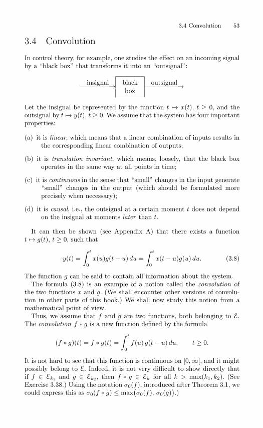
3.4 Convolution 53
3.4 Convolution
In control theory, for example, one studies the effect on an incoming signalby a “black box” that transforms it into an “outsignal”:
insignal black outsignal→ →box
Let the insignal be represented by the function t → x(t), t ≥ 0, and theoutsignal by t → y(t), t ≥ 0. We assume that the system has four importantproperties:
(a) it is linear, which means that a linear combination of inputs results inthe corresponding linear combination of outputs;
(b) it is translation invariant, which means, loosely, that the black boxoperates in the same way at all points in time;
(c) it is continuous in the sense that “small” changes in the input generate“small” changes in the output (which should be formulated moreprecisely when necessary);
(d) it is causal, i.e., the outsignal at a certain moment t does not dependon the insignal at moments later than t.
It can then be shown (see Appendix A) that there exists a functiont → g(t), t ≥ 0, such that
y(t) =∫ t
0x(u)g(t− u) du =
∫ t
0x(t− u)g(u) du. (3.8)
The function g can be said to contain all information about the system.The formula (3.8) is an example of a notion called the convolution of
the two functions x and g. (We shall encounter other versions of convolu-tion in other parts of this book.) We shall now study this notion from amathematical point of view.
Thus, we assume that f and g are two functions, both belonging to E.The convolution f ∗ g is a new function defined by the formula
(f ∗ g)(t) = f ∗ g(t) =∫ t
0f(u) g(t− u) du, t ≥ 0.
It is not hard to see that this function is continuous on [0,∞[, and it mightpossibly belong to E. Indeed, it is not very difficult to show directly thatif f ∈ Ek1 and g ∈ Ek2 , then f ∗ g ∈ Ek for all k > max(k1, k2). (SeeExercise 3.38.) Using the notation σ0(f), introduced after Theorem 3.1, wecould express this as σ0(f ∗ g) ≤ max
(σ0(f), σ0(g)
).)

54 3. Laplace and Z transforms
Convolution can be regarded as an operation for functions, a sort of“multiplication.” For this operation a few simple rules hold; the reader isinvited to check them out:
f ∗ g = g ∗ f (commutative law)f ∗ (g ∗ h) = (f ∗ g) ∗ h (associative law)f ∗ (g + h) = f ∗ g + f ∗ h (distributive law)
Example 3.14. Let f(t) = et, g(t) = e−2t. Then
f ∗ g(t) =∫ t
0eu e−2(t−u) du =
∫ t
0eu−2t+2u du = e−2t
∫ t
0e3u du
= e−2t[ 13 e
3u]u=t
u=0 = 13e
−2t(e3t − 1
)=et − e−2t
3.
Example 3.15. If g(t) = 1, then f ∗g(t) =
∫ t
0 f(u) du. Thus, “integration”can be considered to be convolution with the function 1.
When dealing with convolutions, the Laplace transform is useful becauseof the following theorem.
Theorem 3.6 The Laplace transform of a convolution is the product ofthe Laplace transforms of the two convolution factors:
L[f ∗ g](s) = f(s) g(s).
Proof. Let s be so large that both f(s) and g(s) exist. We have agreedin section 3.1 that this means that the corresponding integrals convergeabsolutely. Now consider the improper double integral∫∫
Q
|f(u)g(v)|e−s(u+v) du dv,
where Q is the first quadrant in the uv plane. The integrated function beingpositive, the integral can be calculated just as we choose. For example, wecan write∫∫
Q
|f(u)g(v)|e−s(u+v) du dv =∫ ∞
0du
∫ ∞
0|f(u)||g(v)|e−sue−sv dv
=∫ ∞
0|f(u)|e−su du
∫ ∞
0|g(v)|e−sv dv.
The two one-dimensional integrals here are assumed to be convergent,which means that the double integral also converges. But this in turn meansthat the improper double integral without modulus signs,
Φ(s) =∫∫
Q
f(u)g(v)e−s(u+v) du dv

3.4 Convolution 55
is absolutely convergent. It can then also be computed in any manner, andwe do it in two ways. One way is imitating the previous calculation:
Φ(s) =∫ ∞
0du
∫ ∞
0f(u)g(v)e−sue−sv dv
=∫ ∞
0f(u)e−su du
∫ ∞
0g(v)e−sv dv = f(s) g(s).
Another way is integrating on triangles DT : u ≥ 0, v ≥ 0, u+ v ≤ T . But∫ T
0f ∗ g(t)e−st dt =
∫ T
0
(∫ t
0f(u)g(t− u) du
)e−su dt
=∫ T
0dt
∫ t
0f(u)e−su g(t− u)e−s(t−u) du
=∫ T
0f(u)e−su du
∫ T
u
g(t− u)e−s(t−u) dt =t− u = vdt = dv
=∫ T
0f(u)e−su du
∫ T−u
0g(v)e−sv dv
=∫∫DT
f(u)g(v)e−sue−sv du dv → Φ(s)
as T → ∞. This proves the formula in the theorem. Example 3.16. As an illustration of the theorem we can take the situationin Example 3.14. There we have
f(s) =1
s− 1, g(s) =
1s+ 2
,
f(s)g(s) =1
(s− 1)(s+ 2)=
13
s− 1−
13
s+ 2= L[f ∗ g](s).
Example 3.17. Find a function f that satisfies the integral equation
f(t) = 1 +∫ ∞
0f(t− u) sinu du, t ≥ 0.
Solution. Suppose that f ∈ E. Then we can transform the equation to get
f(s) =1s
+ f(s) · 1s2 + 1
,
from which we solve
f(s) =s2 + 1s2
· 1s
=s2 + 1s3
=1s
+1s3,

56 3. Laplace and Z transforms
and we see that f(t) = 1 + 12 t
2 ought to be a solution. Indeed it is, be-cause this function belongs to E, and then our successive steps make up asequence of equivalent statements. (It is also possible to check the solutionby substitution in the given integral equation. This should be done, if timepermits.)
Exercises
3.29 Calculate directly the convolution of eat and ebt (consider separately thecases a = b and a = b). Check the result by taking Laplace transforms.
3.30 Use the convolution formula to determine f if f(s) is given by(a) s−1(s+ 1)−1, (b) s−1(s2 + a2)−1.
3.31 Find a function with the Laplace transforms2
(s2 + 1)2.
3.32 Find a function f such that∫ x
0
e−y cos y f(x− y) dy = x2 e−x, x ≥ 0.
3.33 Find a solution of the integral equation∫ t
0
(t− u)2f(u) du = t3, t ≥ 0.
3.34 Find two solutions of the integral equation (3.2) on page 41.
3.35 Find a function y(t) that satisfies y(0) = 0 and
2∫ t
0
(t− u)2 y(u) du+ y′(t) = (t− 1)2 for t > 0.
3.36 Find a function f(t) for t ≥ 0, that satisfies
f(0) = 1, f ′(t) + 3f(t) +∫ t
0
f(u)eu−t du =
0, 0 ≤ t < 2,1, t > 2
.
3.37 Find a solution f of the integral-differential equation
5e−t
∫ t
0
ey cos 2(t− y) f(y) dy = f ′(t) + f(t) − e−t, f(0) = 0.
3.38 Prove the following result: if f ∈ Ek1 and g ∈ Ek2 , then f ∗ g ∈ Ek for allk > maxk1, k2.

3.5 *Laplace transforms of distributions 57
3.5 *Laplace transforms of distributions
Laplace transforms can be used in the study of physical phenomena thattake place in a time interval that starts at a certain moment, at which theclock is set to t = 0. It is possible to allow the functions to include instan-taneous pulses and even more far-reaching generalizations of the classicalnotion of a function – i.e., to allow so-called distributions into the game.When we do so, it will normally be a good thing to allow such things tohappen also at the very moment t = 0, so we modify slightly the definitionof the Laplace transform into the following formula:
f(s) =∫ ∞
0−f(t)e−st dt = lim
ε0
∫ ∞
−ε
f(t)e−st dt.
If f is an ordinary function, the modified definition agrees with the formerone. But if f is a distribution, something new may occur.
As an example, let δa(t) be the Dirac pulse at the point a, where a ≥ 0.Then
δa(s) =∫ ∞
0−δa(t)e−st dt = e−as.
In particular, if a = 0, we get δ(s) = 1. We see that the rule that a Laplacetransform must tend to zero as s → ∞ no longer need hold for transformsof distributions.
The formula for the transform of a derivative must also be slightly mod-ified. Indeed, integration by parts gives
f ′(s) =∫ ∞
0−f ′(t)e−st dt =
[f(t)e−st
]∞
0−+s
∫ ∞
0−f(t)e−st dt = sf(s)−f(0−),
where f(0−) is the left-hand limit of f(t) at 0. This may cause some confu-sion when dealing with functions that are considered to be zero for negativet but nonzero for positive t. In this case it may now happen that f ′ includesa multiple of δ, which explains the different appearance of the formula. Inthis situation, it is preferable to be very explicit in supplying the factorH(t) in the description of functions.
Example 3.18. Solve the initial value problem
y′′ + 4y′ + 13y = δ′(t), y(0−) = y′(0−) = 0.
Solution. Transformation gives
(s2+4s+13)y = s ⇐⇒ y =s
(s+ 2)2 + 9=
s+ 2(s+ 2)2 + 9
− 23· 3(s+ 2)2 + 9
.

58 3. Laplace and Z transforms
The solution is found to be
y(t) = e−2t(cos 3t− 23 sin 3t)H(t).
We check it by differentiating:
y′(t) = e−2t(−2 cos 3t+ 43 sin 3t− 3 sin 3t− 2 cos 3t)H(t) + δ(t)
= e−2t(−4 cos 3t− 53 sin 3t)H(t) + δ(t),
y′′(t) = e−2t(8 cos 3t+ 103 sin 3t+ 12 sin 3t− 5 cos 3t)H(t) − 4δ(t) + δ′(t)
= e−2t(3 cos 3t+ 463 sin 3t)H(t) − 4δ(t) + δ′(t).
Substituting this into the left-hand member of the equation, one sees thatit indeed solves the problem. Example 3.19. Find the general solution of the differential equationy′′ + 3y′ + 2y = δ.
Solution. It should be wellknown that the solution can be written as thesum of the general solution yH of the corresponding homogeneous equationy′′ +3y′ +2y = 0, and one particular solution yP of the given equation. Weeasily find yH = C1e
−t +C2e−2t, and proceed to look for yP . In doing this
we assume that yP (0−) = y′P (0−) = 0, which gives the simplest Laplace
transforms. Indeed, y′P = syP and y′′
P = s2yP , so that
s2yP + 3syP + 2yP = 1 ⇐⇒ yP =1
(s+ 1)(s+ 2)=
1s+ 1
− 1s+ 2
.
Thus it turns out that
yP =(e−t − e−2t
)H(t).
This means that the solution of the given problem is
y =C1e−t + C2e
−2t +(e−t − e−2t
)H(t)
= (C1+H(t))e−t + (C2−H(t))e−2t
=C1e
−t + C2e−2t, t < 0,
(C1 + 1)e−t + (C2 − 1)e−2t, t > 0.
We can see that in each of the intervals t < 0 and t > 0 these expressionsare solutions of the homogeneous equation, which is in accordance withthe fact that δ = 0 in the intervals. What happens at t = 0 is that theconstants change value in such a way that the first derivative has a jumpdiscontinuity and the second derivative contains a δ pulse (draw pictures!).
The particular solution yP found in the preceding problem is called a
fundamental solution of the equation. Let us now denote it by E; thus,
E(t) =(e−t − e−2t
)H(t).
3.5 *Laplace transforms of distributions 59
It is useful in the following situation. Let f be any function, continuous fort ≥ 0. We want to find a solution of the problem y′′ + 3y′ + 2y = f . If weassume y(0−) = y′(0−) = 0, we get
y =f(s)
s2 + 3s+ 2= f(s) · 1
s2 + 3s+ 2= f(s)E(s).
This means that y can be found as the convolution of f and E:
y(t) = f ∗ E(t) =∫ t
0f(t− u)
(e−u − e−2u
)du.
The fundamental solution thus provides a means for finding a particularsolution for any inhomogeneuous equation with the given left-hand side.
This idea can be applied to any linear differential equation with constantcoefficients. The left-hand member of such an equation can be written inthe form P (D)y, where D is the differentiation operator and P (·) is apolynomial. For example, if P (r) = r2 + 3r + 2, then
P (D)y = (D2 + 3D + 2)y = y′′ + 3y′ + 2y.
The fundamental solution E is, in the general case, the function such that
E(s) =1
P (s), E(t) = 0 for t < 0.
Exercises
3.39 Find a solution of the differential equation y′′′ +3y′′ +3y′ +y = H(t−1)+δ(t− 2), that satisfies y(0) = y′(0) = y′′(0) = 0.
3.40 Solve the differential equation y′′ +4y′ +5y = δ(t), y(t) = 0 for t < 0. Thendeduce a formula for a particular solution of the equation y′′ + 4y′ + 5y =f(t), where f is any continuous function such that f(t) = 0 for t < 0.
3.41 Find fundamental solutions for the following equations: (a) y′′ + 4y = δ,(b) y′′ + 4y′ + 8y = δ, (c) y′′′ + 3y′′ + 3y′ + y = δ.
3.42 Find a function y such that y(t) = 0 for t ≤ 0 and
y′(t) + 3y(t) + 2∫ t
0
y(u) du = 2(H(t− 1) −H(t− 2)
)for t > 0.
3.43 Find a function f(t) such that f(t) = 0 for t < 0 and
e−t
∫ t+
0−f(p) ep dp− f(t) + f ′(t) = δ(t) − t e−t H(t), −∞ < t < ∞.

60 3. Laplace and Z transforms
3.6 The Z transform
In this section we sketch the theory of a discrete analogue of the Laplacetransform. We have so far been considering functions t → f(t), where t is areal variable (mostly thought of as representing time). Now, we shall thinkof t as a variable that only assumes the values 0, 1, 2, . . . , i.e., non-negativeinteger values. In applications, this is sometimes more realistic than con-sidering a continuous variable; it corresponds to taking measurements atequidistant points in time.
A function of an integer variable is mostly written as a sequence of num-bers. This will be the way we do it, at least at the beginning of the section.
Let an∞n=0 be a sequence of numbers. We form the infinite series
A(z) =∞∑
n=0
an
zn=
∞∑n=0
anz−n .
If the series is convergent for some z, then it converges absolutely outside ofsome circle in the complex plane. More precisely, the domain of convergenceis a set of the type |z| > σ, where 0 ≤ σ ≤ ∞. (It may also happen thatthe series converges at certain points on the circle |z| = σ, but this israrely of any importance.) Power series of this kind, that may encompassboth positive and negative powers of z, are called Laurent series. (Aparticular case is Taylor series that do not contain any negative powers of z;in the present situation we are considering a reversed case, with no positivepowers.) A necessary and sufficient condition for the series to converge atall is that there exist constants M and R such that |an| ≤ MRn for alln. This condition is analogous to the condition of exponential growth forfunctions to have a Laplace transform.
The function A(z) is called the Z transform of the sequence an∞n=0.
It can be employed to solve certain problems concerning sequences, in amanner that is largely analogous to the way that Laplace transforms canbe used for solving problems for ordinary functions. Important applicationsoccur in the theory of electronics, systems engineering, and automatic con-trol.
When working with the Z transformation, one should be familiar withthe geometric series. Recall that this is the series
∞∑n=0
wn,
where w is a real or complex number. It is convergent precisely if |w| < 1,and its sum is then 1/(1−w). This fact is used “in both directions,” as thefollowing example shows.

3.6 The Z transform 61
Example 3.20. If an = 1 for all n ≥ 0, the Z transform is
∞∑n=0
1zn
=∞∑
n=0
(1z
)n=
1
1 − 1z
=z
z − 1,
which is convergent for all z such that |z| > 1. On the other hand, if λ is anonzero complex number, we can rewrite the function B(z) = z/(z − λ) inthis way:
B(z) =z
z − λ=
1
1 − λ
z
=∞∑
n=0
(λz
)n=
∞∑n=0
λn
zn, |z| > |λ|,
which shows that B(z) is the transform of the sequence bn = λn (n ≥ 0).(Here we actually use the fact that Laurent expansions are unique, whichimplies that two different sequences cannot have the same transform.)
We next present a simple, but typical, problem where the transform canbe used.
Example 3.21. If we know that a0 = 1, a1 = 2 and
an+2 = 3an+1 − 2an , n = 0, 1, 2, . . . , (3.9)
find a formula for an.An equation of the type (3.9) is often called a difference equation. In many
respects, it is analogous to a differential equation: if differential equationsare used for the description of processes taking place in “continuous time,”difference equations can do the corresponding thing in “discrete time.”
To solve the problem in Example 3.21, we multiply the formula (3.9) byz−n and add up for n = 0, 1, 2, . . .:
∞∑n=0
an+2z−n = 3
∞∑n=0
an+1z−n − 2
∞∑n=0
anz−n. (3.10)
Now we introduce the Z transform of the sequence an∞n=0:
A(z) =∞∑
n=0
anz−n = 1 +
2z
+a2
z2 +a3
z3 + · · · . (3.11)
We notice that, firstly,
∞∑n=0
an+1z−n =
∞∑k=1
akz−(k−1) = z
( ∞∑k=1
akz−k
)= z
( ∞∑n=0
anz−n − a0
)= z(A(z) − 1),
and, secondly,
62 3. Laplace and Z transforms
∞∑n=0
an+2z−n =
∞∑k=2
akz−(k−2) = z2
( ∞∑k=2
akz−k
)
= z2
( ∞∑n=0
anz−n − a0 − a1
z
)= z2
(A(z) − 1 − 2
z
).
Thus, the equation (3.10) can be written as
z2(A(z) − 1 − 2
z
)= 3z(A(z) − 1) − 2A(z),
from which A(z) can be solved. After simplification we have
A(z) =z
z − 2.
We saw in the preceding example that this is the Z transform of the se-quence
an = 2n, n = 0, 1, 2, . . . .
We can check the result by returning to the statement of the problem:a0 = 1 and a1 = 2 are all right; and if an = 2n and an+1 = 2n+1, then
3an+1 − 2an = 3 · 2n+1 − 2 · 2n = 3 · 2n+1 − 2n+1 = 2 · 2n+1 = 2n+2,
which is also right. In the example, it is obvious from the beginning that the solution is
unique. If a0 and a1 are given, the formula (3.9) produces the subsequentvalues of the an in an unequivocal way. In general, problems about numbersequences are often uniquely determined in the same manner. However,just as for the Laplace transform, the Z transform cannot be expected togive solutions if these are very fast-growing sequences.
We take a closer look at the correspondence between sequences an∞n=0
and their Z transforms A(z). In order to have an efficient notation we writea = an∞
n=0 and A = Z[a]. Thus, Z denotes a mapping from (a subset of)the set of number sequences to the set of Laurent series convergent outsideof some circle.
Example 3.22. We have already seen that if a = λn∞0 , then
Z[a](z) =∞∑
n=0
λnz−n =z
z − λ, |z| > |λ|.
Example 3.23. If a = 1/n!∞0 , then Z[a](z) =
∞∑n=0
z−n
n!= e1/z, |z| > 0.

3.6 The Z transform 63
Example 3.24. The sequence a = n!∞0 has no Z transform, because
the series∞∑
n=0
n! z−n diverges for all z.
As stated at the beginning of this section, a sufficient (and actually nec-essary) condition for A(z) to exist is that the numbers an grow at mostexponentially: |an| ≤ MRn for some numbers M and R. It is easy tosee that this condition implies the convergence of the series for all z with|z| > R.
Some computational rules for the transformation Z have been collected inthe following theorem. In the interest of brevity we introduce some notationfor operations on number sequences (which can be viewed as functions N →C). If we let a = an∞
n=0 and b = bn∞n=0, we write a+ b = an + bn∞
n=0;and if furthermore λ is a complex number, we put λa = λan∞
n=0. We alsoagree to write
A = Z[a], B = Z[b].
The “radius of convergence” of the Z transform of a is denoted by σa:this means that the series is convergent for |z| > σa (and divergent for|z| < σa).
Theorem 3.7 (i) The transformation Z is linear, i.e.,
Z[λa](z) = λZ[a](z), |z| > σa,
Z[a+ b](z) = Z[a](z) + Z[b](z), |z| > max(σa, σb).
(ii) If λ is a complex number and bn = λnan, n = 0, 1, 2, . . ., then
B(z) = A(z/λ), |z| > λσa.
(iii) If k is a fixed integer > 0 and bn = an+k, n = 0, 1, 2, . . ., then
B(z) = zk
(A(z) − a0 − a1
z− · · · − ak−1
zk−1
)= zkA(z) − a0z
k − a1zk−1 − · · · − ak−1z, |z| > σa.
(iv) Conversely, if k is a positive integer and bn = an−k for n ≥ k andbn = 0 for n < k, then B(z) = z−kA(z).
(v) If bn = nan, n = 0, 1, 2, . . ., then
B(z) = −z A′(z), |z| > σa.
Proof. The assertions follow rather immediately from the definitions. Wesaw a couple of cases of (iii) in Example 3.21 above. We content ourselvesby sketching the proofs of (ii) and (v). For (ii) we find
B(z) =∞∑
n=0
bnz−n =
∞∑n=0
λnanz−n =
∞∑n=0
an
(z
λ
)−n
= A(z/λ).

64 3. Laplace and Z transforms
And as for (v), the right-hand side is
−z· ddz
∞∑n=0
anz−n = −z
∞∑n=0
(−n)anz−n−1 =
∞∑n=0
nanz−n = left-hand side.
Example 3.25. Example 3.23 and rule (ii) give us the transform of thesequence λn/n!∞
0 , viz.,
Λ(z) = e1/(z/λ) = eλ/z.
When solving problems concerning the Z transform, you should have a
table at hand, containing rules of computation as well as actual transforms.Such a table is included at the end of this book (p. 250).
Example 3.26. Find a formula for the so-called Fibonacci numbers,which are defined by f0 = f1 = 1, fn+2 = fn+1 + fn for n ≥ 0.
Solution. Let F = Z[f ]. If we Z-transform the recursion formula, using (iii)from the theorem, we get
z2F (z) − z2 − z = (zF (z) − z) + F (z),
whence (z2 − z − 1)F (z) = z2 and
F (z) =z2
z2 − z − 1= z · z
z2 − z − 1.
In order to recover fn, a good idea would be to expand into partial fractions,in the hope that simple expressions could be looked up in the table onpage 250. A closer look at this table reveals, however, that it would be agood thing to have a z in the numerator of the partial fractions, insteadof just a constant. Thus, here we have peeled off a factor z from F (z) andproceed to expand the remaining expression:
F (z)z
=z
z2 − z − 1=
A
z − α+
B
z − β,
where
α =1 +
√5
2, β =
1 − √5
2, A =
√5 + 12√
5, B =
√5 − 12√
5.
This gives
F (z) =Az
z − α+
Bz
z − β
3.6 The Z transform 65
and from the table we conclude that
fn = Aαn +Bβn =√
5 + 12√
5
(1 +
√5
2
)n
+√
5 − 12√
5
(1 − √
52
)n
.
This can be rewritten as
fn =1√5
[(1 +
√5
2
)n+1
−(
1 − √5
2
)n+1], n = 0, 1, 2, . . . .
(In spite of all the appearances of√
5 in the expression, it is an integer forall n ≥ 0.)
As you can see in this example, the method of expanding rational func-tions into partial fractions can be useful in dealing with Z transforms,provided one starts out by securing an extra factor z to be reintroduced inthe numerators after the expansion.
If a and b are two number sequences, we can form a third sequence, c,called the convolution of a and b, by writing
cn =n∑
k=0
an−kbk =n∑
k=0
akbn−k, n = 0, 1, 2, . . . .
One writes c = a ∗ b, and we also permit ourselves to write things likecn = (a ∗ b)n. We determine the Z transform C = Z[c]:
C(z) =∞∑
n=0
n∑k=0
an−kbk z−n =
∞∑k=0
∞∑n=k
an−kbk z−n
=∞∑
k=0
∞∑n=k
an−kz−(n−k) bkz
−k =∞∑
k=0
bkz−k
∞∑n=k
an−kz−(n−k)
=∞∑
k=0
bkz−k
∞∑m=0
amz−m = A(z)B(z).
The manipulations of the double series are permitted for |z| > max(σa, σb),because in that region everything converges absolutely.
This notion of convolution appears in, e.g., control theory, if a system isconsidered in discrete time (see Appendix A).
Example 3.27. Find x(t), t = 0, 1, 2, . . ., from the equation
t∑k=0
3−k x(t− k) = 2−t, t = 0, 1, 2, . . . .

66 3. Laplace and Z transforms
Solution. The left-hand side is the convolution of x and the function t →(1/3)t, so that taking Z transforms of both members gives
z
z − 13
·X(z) =z
z − 12
.
(We have used the result of Example 3.22.) We get
z) =z − 1
3
z − 12
=z
z − 12
− 13 · 1
z − 12
,
and, using Example 3.22 and rule (iv) of Theorem 3.7, we see that
x(t) =
1 for t = 0,( 1
2
)t − 13 · ( 1
2
)t−1 for t ≥ 1.
The final expression can be rewritten as
x(t) =( 1
2 − 13
) · ( 12
)t−1 = 16 · 21−t = 1
3 · 2−t, t ≥ 1.
In a final example, we indicate a way of viewing the Z transform as
a particular case of the Laplace transform. Here we use translates of theDirac delta “function,” as in Sec. 3.5.
Example 3.28. Let an∞n=0 be a sequence having a Z transform A(z),
and define a function f by
f(t) =∞∑
n=0
anδn(t) =∞∑
n=0
anδ(t− n).
The convergence of this series is no problem, because for any particular tat most one of the terms is different from zero. Its Laplace transform mustbe
f(s) =∞∑
n=0
∫ ∞
0−e−stanδ(t− n) dt =
∞∑n=0
ane−ns =
∞∑n=0
an
(es)−n = A(es).
Thus, via a change of variable z = es, the two transforms are more or lessthe same thing.
Exercises3.44 Determine the Z transforms of the following sequences an∞
n=0 :
(a) an =12n
(b) an = n · 3n (c) an = n2 · 2n
(d) an =
(n
p
)=n(n− 1) · · · (n− p+ 1)
p!for n ≥ p, = 0 for 0 ≤ n ≤ p (p
is a fixed integer).

3.7 Applications in control theory 67
3.45 Determine the sequence a = an∞n=0, if its Z transform is (a) A(z) =
z
3z − 2, (b) A(z) =
1z
.
3.46 Determine the numbers an and bn, n = 0, 1, 2, . . ., if a0 = 0, b0 = 1 andan+1 + bn = −2n,an + bn+1 = 1,
n = 0, 1, 2, . . . .
3.47 Find the numbers an and bn, n = 0, 1, 2, . . ., if a0 = 0, b0 = 1 andan+1 + bn = 2,an − bn+1 = 0,
n = 0, 1, 2, . . . .
3.48 Find an, n = 0, 1, 2, . . ., such that a0 = a1 = 0 and an+2 − 3an+1 + 2an =1 − 2n for n = 0, 1, 2, . . ..
3.49 Find an, n = 0, 1, 2, . . ., if a0 = a1 = 0 and
an+2 + 2an+1 + an = (−1)nn, n = 0, 1, 2, . . . .
3.50 Find an, n = 0, 1, 2, . . ., if a0 = 1, a1 = 3 and an+2 + an = 2n + 4 whenn ≥ 0.
3.51 Determine the numbers y(t) for t = 0, 1, 2, . . . , so that
t∑k=0
(t− k) 3t−k y(k) =
0, t = 0,1, t = 1, 2, 3, . . . .
3.52 Find an for n ≥ 0, if a0 = 0 andn∑
k=0
kan−k − an+1 = 2n for n ≥ 0.
3.53 Determine x(n) for n = 0, 1, 2, . . ., so that
x(n) + 2n∑
k=0
(n− k)x(k) = 2n, n = 0, 1, 2, . . . .
3.7 Applications in control theory
We return to the “black box” of Sec. 3.4 (p. 53). Such a box can often bedescribed by a differential equation of the type P (D)y(t) = x(t), where x isthe input and y the output. If x(t) is taken to be a unit pulse, x(t) = δ(t),the solution y(t) with y(t) = 0 for t < 0 is called the pulse response, orimpulse response, of the black box. The pulse response is the same thing asthe fundamental solution. In the general case, Laplace transformation willgive P (s)y(s) = 1 and thus y(s) = 1/P (s). The function
G(s) =1
P (s)

68 3. Laplace and Z transforms
is called the transfer function of the box. When solving the general problem
P (D)y(t) = x(t), y(t) = 0 for t < 0,
Laplace transformation will now result in
P (s)y(s) = x(s)
ory(s) = G(s)x(s).
This formula is actually the Laplace transform of the convolution formula(3.8) of page 53. It provides a quick way of finding the outsignal y toany insignal x. The function g in the convolution is actually the impulseresponse.
In control theory, great importance is attached to the notion of stability.A black box is stable, if its impulse response is transient, i.e., g(t) tendsto zero as time goes by. This means that disturbances in the input willaffect the output only for a short time and will not accumulate. If P (s) isa polynomial, the impulse response will be transient if and only if all itszeroes have negative real parts.
Example 3.29. The polynomial P1(s) = s2 + 2s + 2 has zeroes s =−1±i. Both have real part −1, so that the device described by the equationy′′+2y′+2y = x(t) is stable. In contrast, the polynomial P2(s) = s2+2s−1has zeroes s = −1 ± √
2. One of these is positive, which implies that thecorresponding black box is unstable. Finally, the polynomial P3(s) = s2 +1has zeroes s = ±i. These have real part zero; the impulse reponse is g(t) =sin t, which is not transient. The situation is considered as unstable. (It isunstable also inasmuch as a small disturbance of the coefficients of P3(s)can cause the zeroes to move into the right half-plane, which gives rise toexponentially growing solutions.)
So far, we have assumed that the black box is described in continuoustime. In the real world, it is often more realistic to assume that time isdiscrete, i.e., that input and output are sampled at equidistant points intime. For simplicity, we assume that the sampling is done at t = 0, 1, 2, . . .,and that the input signal x(t) and the output y(t) are both zero for t < 0.Then, of course, the Z transform is the adequate tool.
A black box is often described by a difference equation of the type
y(t+k)+ak−1y(t+k−1)+· · ·+a2y(t+2)+a1y(t+1)+a0y(t) = x(t), t ∈ Z.(3.12)
We introduce the characteristic polynomial
P (z) = zk + ak−1zk−1 + · · · + a2z
2 + a1z + a0.
We assumed that x(t) and y(t) were both zero for negative t. Puttingt = −k in (3.12), we find that
y(0) = x(−k) − ak−1y(−1) − · · · − a1y(−k + 1) − a0y(−k),
3.7 Applications in control theory 69
which implies that also y(0) = 0. Consequently, putting t = −k + 1, alsoy(1) = 0, and so on. Not until we have an x(t) that is different fromzero do we find a y(t + k) different from zero. Thus we have initial valuesy(0) = · · · = y(k − 1) = 0. By the rules for the Z transform, we can theneasily transform the equation (3.12). With obvious notation we get
P (z)Y (z) = X(z).
Thus,
Y (z) =X(z)P (z)
= G(z)X(z),
where G(z) = 1/P (z) is the transfer function. Just as in the previoussituation, it is also the impulse response, because it is the output resultingfrom inputting the signal
δ(t) = 1 for t = 0, δ(t) = 0 otherwise.
The stability of equation (3.12) hinges on the localization of the zeroesof the polynomial P (z). As can be seen from a table of Z transforms, azero a of P (z) implies that the solution contains terms involving at. Thuswe have stability precisely if all the zeroes of P (z) are in the interior of theunit disc |z| < 1.
Example 3.30. The difference equation y(t+2)+ 12y(t+1)+ 1
4y(t) = x(t)has P (z) = z2+ 1
2z+14 with zeroes z = − 1
4 ±√
34 i. These satisfy |z| = 1
2 < 1,so that the equation is stable. The equation
y(t+ 3) + 2y(t+ 2) − y(t+ 1) + 2y(t) = x(t)
is unstable. This can be seen from the constant term (= 2) of the char-acteristic polynomial; as is well known, this term is (plus or minus) theproduct of the zeroes, which implies that these cannot all be of modulusless than one.
More sophisticated methods for localizing the zeroes of polynomials canbe found in the literature on complex analysis and in books dealing withthese applications.
Exercises
3.54 Investigate the stability of the following equations:(a) y′′+2y′+3y = x(t), (b) y′′′+3y′′+3y′+y = x(t), (c) y′′+4y = x(t).
3.55 Are these difference equations stable or unstable?(a) 2y(t+ 2) − 2y(t+ 1) + y(t) = x(t),(b) y(t+ 2) − y(t+ 1) + y(t) = x(t),(c) 2y(t+ 3) − y(t+ 2) + 3y(t+ 1) + 3y(t) = x(t).
70 3. Laplace and Z transforms
Summary of Chapter 3
To provide an overview of the results of this chapter, we collect the main defini-tions and theorems here. The precise details of the conditions for the validity ofthe results are sometimes indicated rather sketchily. Thus, this summary shouldserve as a memory refresher. Details should be looked up in the core of the text.Facts that rather belong in a table of transforms, such as rules of computation,are not included here, but can be found at the end of the book (p. 247 ff).
DefinitionIf f(t) is defined for t ∈ R and f(t) = 0 for t < 0, its Laplace transform isdefined by
f(s) =∫ ∞
0f(t)e−st dt,
provided the integral is abolutely convergent for some value of s.
TheoremFor f to exist it is sufficient that f grows at most exponentially, i.e., that|f(t)| ≤ Mekt for some constants M and k.
TheoremIf f(s) = g(s) for all (sufficiently large) s, then f(t) = g(t) for all t whereboth f and g are continuous.
TheoremIf we define the convolution h = f ∗ g by
h(t) = f ∗ g(t) =∫ t
0f(t− u)g(u) du =
∫ t
0f(u)g(t− u) du,
then its Laplace transform is h = f g.
DefinitionIf an∞
n=0 is a sequence of numbers, its zeta transform is defined by
A(z) =∞∑
n=0
anz−n,
provided the series is convergent for some value of z. This holds if |an| ≤MRn for some constants M and R.
Historical notes
The Laplace transform is, not surprisingly, found in the works of Pierre Simonde Laplace, notably his Theorie analytique des probabilites of 1812. In this book,he made free use of Laplace transforms and also generating functions (which arerelated to the Z transform) in a way that baffled his contemporaries. During the

Problems for Chapter 3 71
nineteenth century, the technique was developed further, and also influenced bysimilar ideas such as the “operational calculus” of Oliver Heaviside (Britishphysicist and applied mathematician, 1850–1925). With the development of mod-ern technology in computing and control theory, the importance of these methodshas grown enormously.
Problems for Chapter 3
3.56 Solve the system y′ − 2z = (1 − t)e−t, z′ + 2y = 2te−t, t > 0, with initialconditions y(0) = 0, z(0) = 1.
3.57 Solve the problem y′′ + 2y′ + 2y = 5et, t > 0; y(0) = 1, y′(0) = 0.
3.58 Solve the problem y′′′ + y′′ + y′ − 3y = 1, t > 0, when y(0) = y′(0) = 0,y′′(0) = 1.
3.59 Solve the problem y′′ + 4y = f(t), t > 0; y(0) = 0, y′(0) = 1, where
f(t) =
(t− 1)2, t ≥ 10, 0 < t < 1.
3.60 Find y = y(t) for t > 0 that solves y′′−4y′+5y = ϕ(t), y(0) = 2, y′(0) = 0,where ϕ(t) = 0 for t < 2, ϕ(t) = 5 for t > 2.
3.61 Find f(t) for t ≥ 0, such that f(0) = 1 and
8∫ t
0
f(t− u) e−u du+ f ′(t) − 3f(t) + 2e−t = 0, t > 0.
3.62 Let f be the function described by
f(t) = 0, t ≤ 0; f(t) = t, 0 < t ≤ 1; f(t) = 1, t > 1.
Solve the differential equation y′′(t)+y(t) = f(t) with initial values y(0) =0, y′(0) = 1.
3.63 Solve y′′′ + y′ = t− 1, y(0) = 2, y′(0) = y′′(0) = 0.
3.64 Solve y′′′ + 3y′′ + 3y′ + y = t+ 3, t > 0; y(0) = 0, y′(0) = 1, y′′(0) = 2.
3.65 Solve the initial value problemz′′ − y′ = e−t,
y′′ + y′ + z′ + z = 0,t > 0;
y(0) = 0, y′(0) = 1;z(0) = 0, z′(0) = −1.
3.66 Find f such that f(0) = 1 and
2e−t
∫ t
0
(t− u) eu f(u) du+ f ′(t) + 2t2e−t = 0.
3.67 Solve the problemy′′(t) + 2z′(t) − y(t) = 4et,
z′′(t) − 2y′(t) − z(t) = 0,t > 0;
y(0) = 0, y′(0) = 2,z(0) = z′(0) = 0.

72 3. Laplace and Z transforms
3.68 Solve y′′′ + y′′ + y′ + y = 4e−t, t > 0; y(0) = 0, y′(0) = 3, y′′(0) = −6.
3.69 Find f that solves∫ t
0
f(u)(t− u) sin(t− u) du− 2f ′(t) = 12e−t, t > 0; f(0) = 6.
3.70 Solve y′′′ + 3y′′ + y′ − 5y = 0, t > 0; y(0) = 1, y′(0) = −2, y′′(0) = 3.
3.71 Solve y′′′(t) + y′′(t) + 4y′(t) + 4y(t) = 8t + 4, t > 0, with initial valuesy(0) = −1, y′(0) = 4, y′′(0) = 0.
3.72 Solve y′′′ + y′′ + y′ + y = 2e−t, t > 0; y(0) = 0, y′(0) = 2, y′′(0) = −2.
3.73 Find a solution y = y(t) for t > 0 to the initial value problem y′′ + 2ty′ −4y = 1, y(0) = y′(0) = 0.
3.74 Find a solution of the partial differential equation utt +2ut +xux +u = xtfor x > 0, t > 0, such that u(x, 0) = ut(x, 0) = 0 for x > 0 and u(0, t) = 0for t > 0.
3.75 Use Laplace transformation to find a solution of
y′′(t) − ty′(t) + y(t) = 5, t > 0; y(0) = 5, y′(0) = 3.
3.76 Find f such that f(t) = 0 for t < 0 and
5e−t
∫ t
0
ey cos 2(t− y) f(y) dy = f ′(t) + f(t) − e−t, t > 0.
3.77 Solve the integral equation y(t) +∫ t
0(t− u) y(u) du = 3 sin 2t.
3.78 Solve the difference equation an+2 − 2an+1 +an = bn for n ≥ 0 with initialvalues a0 = a1 = 0 and right-hand member (a) bn = 1, (b) bn = en,(c) b0 = 1, bn = 0 for n > 0.

4Fourier series
4.1 Definitions
We are going to solve, as far as we can, the approximation problem thatwas presented in Sec. 1.4. The strategy will perhaps appear somewhatsurprising: starting from a function f , we shall define a certain series, andin due time we shall find that the function can be recovered from this seriesin various ways.
All functions that we consider will have period 2π. The whole theorycould just as well be carried through for functions having some other period.This is equivalent to the standard case that we treat, via a simple lineartransformation of the independent variable. The formulae that hold in thegeneral case are collected in Sec. 4.5.
A function defined on R with period 2π can alternatively be thought ofas defined on the unit circle T, the variable being the polar coordinate.We shall frequently take this point of view. For example, the integral of fover an interval of one period can be written
∫T f(t) dt. When we want to
compute this integral, we can choose any convenient period interval for theactual calculations:
∫T
=∫ π
−π
=∫ 2π
0=∫ a+2π
a
, a ∈ R.
(If T is viewed as a circle, the integral∫T f(t) dt is not to be considered as a
line integral of the sort used to calculate amounts of work in mechanics, or

74 4. Fourier series
that appears in complex analysis. Instead, it is a line integral with respectto arc length.)
One must be careful when working on T and speaking of notions such ascontinuity. The statement that f ∈ C(T) must mean that f is continuous atall points of the circle. If we switch to viewing f as a 2π-periodic function,this function must also be continuous. The formula f(t) = t for −π < t < π,for instance, defines a function that cannot be made continuous on T: atthe point on T that corresponds to t = ±π, the limits of f(t) from differentdirections are different.
Similar care must be taken when speaking of functions belonging toCk(T), i.e., having continuous derivatives of orders up to and includingk. As an example, the definition g(t) = t2, |t| ≤ π, describes a functionthat is in C(T), but not in C1(T). The first derivative does not exist att = ±π. This can be seen graphically by drawing the periodic continuation,which has corners at these points (sketch a picture!).
Let us now do a preparatory maneuver. Suppose that a function f is thesum of a series
f(t) =∞∑
n=−∞cn e
int =∑n∈Z
cn eint. (4.1)
We assume that the coefficients cn are complex numbers such that∑n∈Z
|cn| < ∞.
By the Weierstrass M -test, the series actually converges absolutely anduniformly, since |eint| is always equal to 1. Each term of the series is con-tinuous and has period 2π, and the sum function f inherits both theseproperties.
Now let m be any integer (positive, negative, or zero), and multiply theseries by e−imt. It will still converge uniformly, and it can be integratedterm by term over a period, such as the interval (−π, π):
π∫−π
f(t) e−imt dt =
π∫−π
∑n∈Z
cn ei(n−m)t dt =
∑n∈Z
cn
∫ π
−π
ei(n−m)t dt.
But it is readily seen that∫ π
−π
eikt dt =
2π, k = 0,0, k = 0.
It follows that all the terms in the sum vanish, except the one where n−m =0, which is the same thing as n = m, and the result is that∫ π
−π
f(t) e−imt dt = 2πcm.
4.1 Definitions 75
Thus, for an absolutely convergent series of the form (4.1), the coefficientscan be computed from the sum function using this formula. This fact canbe taken as a motivation for the following definition.
Definition 4.1 Let f be a function with period 2π that is absolutely Rie-mann-integrable over a period. Define the numbers cn, n ∈ Z, by
cn =12π
∫Tf(t) e−int dt =
12π
∫ π
−π
f(t) e−int dt.
These numbers are called the Fourier coefficients of f , and the Fourierseries of f is the series ∑
n∈Z
cn eint.
Notice that the definition does not state anything about the convergenceof the series, even less what its sum might be if it happens to converge. Itis the main task of this chapter to investigate these questions.
When dealing simultaneously with several functions and their Fouriercoefficients it is convenient to indicate to what function the coefficients be-long by writing things like cn(f). Another commonly used way of denotingthe Fourier coefficients of f is f(n).
When we want to state, as a formula, that f has a certain Fourier series,we write
f(t) ∼∑n∈Z
cn eint.
This means nothing more or less than the fact that the numbers cn arecomputable from f using certain integrals.
There are a number of alternative ways of writing the terms in a Fourierseries. For instance, when dealing with real-valued functions, the complex-valued functions eint are often felt to be rather “unnatural.” One can thenwrite eint = cosnt + i sinnt and reshape the two terms corresponding to±n like this:
cneint + c−ne
−int = cn(cosnt+ i sinnt) + c−n(cosnt− i sinnt)= (cn + c−n) cosnt+ i(cn − c−n) sinnt = an cosnt+ bn sinnt,
n = 1, 2, . . . .
In the special case n = 0 we have only one term, c0. This gives a series ofthe form
c0 +∞∑
n=1
(an cosnt+ bn sinnt).
The coefficients in this series are given by new integral formulae:
an = cn + c−n =12π
∫Tf(t)e−int dt+
12π
∫Tf(t)eint dt

76 4. Fourier series
=1π
∫Tf(t) 1
2 (eint + e−int) dt =1π
∫Tf(t) cosnt dt, n = 1, 2, 3, . . . ,
and similarly one shows that
bn =1π
∫Tf(t) sinnt dt, n = 1, 2, 3, . . . .
If we extend the validity of the formula for an to n = 0, we find thata0 = 2c0. For this reason the Fourier series is commonly written
f(t) ∼ 12a0 +
∞∑n=1
(an cosnt+ bn sinnt). (4.2)
This is sometimes called the “real” or trigonometric version of the Fourierseries for f . It should be stressed that this is nothing but a different wayof writing the series — it is really the same series as in the definition.
The terms in the series (4.2) can be interpreted as vibrations of differ-ent frequencies. The constant term 1
2 a0 is a “DC component,” the terma1 cos t + b1 sin t has period 2π, the term with n = 2 has half the periodlength, for n = 3 the period is one-third of 2π, etc. These terms can bewritten in yet another way, that emphasizes this physical interpretation.The reader should be familiar with the fact that the sum of a cosine anda sine with the same period can always be rewritten as a single cosine (orsine) function with a phase angle:
a cosnt+ b sinnt=√a2 + b2
(a√
a2 + b2cosnt+
b√a2 + b2
sinnt)
=√a2 + b2(cosα cosnt+ sinα sinnt) =
√a2 + b2 cos(nt− α),
where the phase angle α is a number such that cosα = a/√a2 + b2, sinα =
b/√a2 + b2. This means that (4.2) can be written in the form
∞∑n=0
An cos(nt− αn). (4.3)
This is sometimes called the physical version of the Fourier series. In thisformula one can immediately see the amplitude An of each partial fre-quency. In this text, however, we shall not work with this form of theseries, since it is slightly unwieldy from a mathematical point of view.
When asked to compute the Fourier series of a specific function, it isnormally up to the reader to choose what version to work with. This isillustrated by the following examples.
Example 4.1. Define f by saying that f(t) = et for −π < t < π andf(t + 2π) = f(t) for all t. (This leaves f(t) undefined for t = (2n + 1)π,

4.1 Definitions 77
π−π
10
t
FIGURE 4.1.
but this does not matter. The value of a function at one point or anotherdoes not affect the values of its Fourier coefficients!) We get a function withperiod 2π (see Figure 4.1). Its Fourier coefficients are
cn =12π
∫ π
−π
et e−int dt =12π
∫ π
−π
e(1−in)t dt =12π
[e(1−in)t
1 − in
]π
t=−π
=eπ−inπ − e−π+inπ
2π(1 − in)=
(−1)n(eπ − e−π)2π(1 − in)
=(−1)n sinhππ(1 − in)
.
Here we used the fact that e±inπ = (−1)n. Now we can write
f(t) ∼ 1π
∑n∈Z
(−1)n sinhπ1 − in
eint =sinhππ
∑n∈Z
(−1)n
1 − ineint.
We remind the reader of a couple of notions of symmetry that turn out
to be useful in connection with Fourier series. A function f defined on Ris said to be even, if f(−t) = f(t) for all t ∈ R. A function f is odd,if f(−t) = −f(t). (The terms should bring to mind the special functionf(t) = tn, which is even if n is an even integer, odd if n is an odd integer.)An odd function f on a symmetric interval (−a, a) has the property thatthe integral over (−a, a) is equal to zero. This has useful consequencesfor the so-called real Fourier coefficients an and bn. If f is even and hasperiod 2π, the sine coefficients bn will be zero, and furthermore the cosinecoefficients will be given by the formula
f even ⇒ an =2π
∫ π
0f(t) cosnt dt.
In an analogous way, an odd function has all cosine coefficients equal tozero, and its sine coefficients are given by
f odd ⇒ bn =2π
∫ π
0f(t) sinnt dt.

78 4. Fourier series
t
FIGURE 4.2.
When computing the Fourier series for an even or odd function these factsare often useful.
Example 4.2. Let f be an odd function with period 2π, that satisfiesf(t) = (π − t)/2 for 0 < t < π. Find its Fourier series! (See Figure 4.2.)
Solution. Notice that the description as given actually determines the func-tion completely (except for its value at one point in each period, which doesnot matter). Because the function is odd we have an = 0 and
bn =2π
∫ π
0
π − t
2sinnt dt
=1π
[(π − t)
− cosntn
]π
t=0+
1nπ
∫ π
0(−1) cosnt dt
=1n
− 1n2π
[sinnt
]π
t=0=
1n.
Thus,
f(t) ∼∞∑
n=1
sinntn
.
Example 4.3. Let f(t) = t2 for |t| ≤ π and define f outside of thisinterval by proclaiming it to have period 2π (draw a picture!). Find theFourier series of this function.
Solution. Now the function is even, and so bn = 0 and
an =2π
∫ π
0t2 cosnt dt
n = 0↓=
2π
[t2
sinntn
]π
0− 2nπ
∫ π
02t sinnt dt
=− 4nπ
[t− cosnt
n
]π
0− 4n2π
∫ π
01 · cosnt dt =
4π cosnπn2π
− 0 =4(−1)n
n2 .
For n = 0 we must do a separate calculation:
a0 =2π
∫ π
0t2 dt =
2π
· π3
3=
2π2
3.

4.1 Definitions 79
Collecting the results we get
f(t) ∼ π2
3+ 4
∞∑n=1
(−1)n
n2 cosnt.
The series obtained in Example 4.3 is clearly convergent; indeed it even
converges uniformly, by Weierstrass. At this stage we cannot tell what itssum is. The goal of the next few sections is to investigate this. For themoment, we can notice two facts about Fourier coefficients:
Lemma 4.1 Suppose that f is as in the definition of Fourier series. Then
1. The sequence of Fourier coefficients is bounded; more precisely,
|cn| ≤ 12π
∫T
|f(t)| dt for all n.
2. The Fourier coefficients tend to zero as |n| → ∞.
Proof. For the cn we have
|cn| =12π
∣∣∣∣∫Tf(t) e−int dt
∣∣∣∣ ≤ 12π
∫T
|f(t)||e−int| dt =12π
∫T
|f(t)| dt = M,
where M is a fixed number that does not depend on n. (In just the sameway one can estimate an and bn.) The second assertion of the lemma is justa case of Riemann–Lebesgue’s lemma.
The constant term in a Fourier series is of particular interest:
c0 =a0
2=
12π
∫ π
−π
f(t) dt.
This can be interpreted as the mean value of the function f over one period(or over T). This can often be useful in problem-solving. It is also intuitivelyreasonable in that all the other terms of the series have mean value 0 overany period (think of the graph of, say, sinnt).
Exercises
4.1 Prove the formulae cn = 12 (an − ibn) and c−n = 1
2 (an + ibn) for n ≥ 0(where b0 = 0).
4.2 Assume that f and g are odd functions and h is even. Find out which ofthe following functions are odd or even: f + g, fg, fh, f2, f + h.
4.3 Show that an arbitrary function f on a symmetric interval (−a, a) can bedecomposed as fE + fO, where fE is even and fO is odd. Also show thatthis decomposition is unique. Hint: put fE(t) = (f(t) + f(−t))/2.

80 4. Fourier series
4.4 Determine the Fourier series of the 2π-periodic function described by f(t) =t+ 1 for |t| < π.
4.5 Prove the following relations for a (continuous) function f and its “com-plex” Fourier coefficients cn:(a) If f is even, then cn = c−n for all n.(b) If f is odd, then cn = −c−n for all n.(c) If f is real-valued, then cn = c−n for all n (where denotes complexconjugation).
4.6 Find the Fourier series (in the “real” version) of the functions (a) f(t) =cos 2t, (b) g(t) = cos2 t, (c) h(t) = sin3 t. Sens moral?
4.7 Let f have the Fourier coefficients cn. Prove the following rules forFourier coefficients (F.c.’s):(a) Let a ∈ Z. Then the function t → eiatf(t) has F.c.’s cn−a.(b) Let b ∈ R. Then the function t → f(t− b) has F.c.’s e−inbcn.
4.8 Find the Fourier series of h(t) = e3itf(t − 4), when f has period 2π andsatisfies f(t) = 1 for |t| < 2, f(t) = 0 for 2 < |t| < π.
4.9 Compute the Fourier series of f , where f(t) = e−|t|, |t| < π, f(t + 2π) =f(t), t ∈ R.
4.10 Let f and g be defined on T with Fourier coefficients cn(f) resp. cn(g).Define the function h by
h(t) =12π
∫T
f(t− u) g(u) du.
Show that h is welldefined on T (i.e., h has also period 2π), and prove thatcn(h) = cn(f) cn(g). (The function h is called the convolution of f and g.)
4.2 Dirichlet’s and Fejer’s kernels; uniqueness
It is a regrettable fact that a Fourier series need not be convergent. Forexample, it is possible to construct a continuous function such that itsFourier series diverges at a specified point (see, for example, the book byThomas Korner mentioned in the bibliography). We shall see, in duetime, that if we impose somewhat harder requirements on the function,such as differentiability, the results are more positive.
It is, however, true that the Fourier series of a continuous function isCesaro summable to the values of the function, and this is the main resultof this section.
We start by establishing a closed formula for the partial sums of a Fourierseries. To this end we shall use the following formula:
Lemma 4.2
DN (u) :=1π
(12 +
N∑n=1
cosnu)
=12π
N∑n=−N
einu =sin(N + 1
2 )u2π sin 1
2u.

4.2 Dirichlet’s and Fejer’s kernels; uniqueness 81
Proof. The equality of the two sums follows easily from Euler’s formulae.Let us then start from the “complex” version of the sum and compute itas a finite geometric sum:
2πDN (u) =N∑
n=−N
einu = e−iNu2N∑n=0
einu = e−iNu · 1 − ei(2N+1)u
1 − eiu
= e−iNu · ei(N+ 1
2 )u(e−i(N+ 1
2 )u − ei(N+ 12 )u
)eiu/2
(e−iu/2 − eiu/2
)=e−iNu+i(N+ 1
2 )u
eiu/2 · −2i sin(N + 12 )u
−2i sin 12 u
=sin(N + 1
2 )usin 1
2u.
The function DN is called the Dirichlet kernel. Its graph is shown in
Figure 4.3 on page 87.When discussing the convergence of Fourier series, the natural partial
sums are those containing all frequencies up to a certain value. Thus wedefine the partial sum sN (t) to be
sN (t) := 12 a0 +
N∑n=1
(an cosnt+ bn sinnt) =N∑
n=−N
cneint.
Using the Dirichlet kernel we can obtain an integral formula for this sum,assuming the cn to be the Fourier coefficients of a function f :
sN (t) =N∑
n=−N
cneint =
N∑n=−N
12π
∫ π
−π
f(u) e−inu du · eint
=1π
∫ π
−π
f(u) · 12
N∑n=−N
ein(t−u) du =∫ π
−π
f(u)DN (t− u) du
=12π
∫ π
−π
f(t− u)sin(N + 1
2 )usin 1
2udu.
In the last step we change the variable (t − u is replaced by u) and makeuse of the periodicity of the integrand. We shall presently take another stepand form the arithmetic means of the N + 1 first partial sums. To achievethis we need a formula for the mean of the corresponding Dirichlet kernels:
Lemma 4.3
FN (u) :=1
N + 1
N∑n=0
Dn(u) =1
2π(N + 1)
(sin 1
2 (N + 1)usin 1
2u
)2.

82 4. Fourier series
The proof can be done in a way similar to Lemma 4.2 (or in some otherway). It is left as an exercise. The function FN (t) is called the Fejer kernel.
Now we can form the mean of the partial sums:
σN (t) =s0(t) + s1(t) + · · · + sN (t)
N + 1=
1N + 1
N∑n=0
∫ π
−π
f(t− u)Dn(u) du
=∫ π
−π
f(t− u) · 1N + 1
N∑n=0
Dn(u) du =∫ π
−π
f(t− u)FN (u) du.
Lemma 4.4 The Fejer kernel FN (u) has the following properties:
1. FN is an even function, and FN (u) ≥ 0.
2.∫ π
−πFN (u) du = 1.
3. If δ > 0, then limN→∞∫ π
δFN (u) du = 0.
Proof. Property 1 is obvious. Number 2 follows from∫ π
−π
Dn(u) du =1π
∫ π
−π
( 12 +cosu+· · ·+cosnu
)du = 1, n = 0, 1, 2, . . . , N,
and the fact that FN is the mean of these Dirichlet kernels. Finally, property3 can be proved thus:
0 ≤∫ π
δ
FN (u) du =1
2π(N + 1)
∫ π
δ
sin2 12 (N + 1)usin2 1
2udu
≤ 12π(N + 1)
∫ π
δ
1sin2 1
2δdu =
12π(N + 1)
π − δ
sin2 12δ
=Cδ
N + 1→ 0
as N → ∞. The lemma implies that FN∞
N=1 is a positive summation kernel suchas the ones studied in Sec. 2.4. Applying Corollary 2.1 we then have theresult on Cesaro sums of Fourier series.
Theorem 4.1 (Fejer’s theorem) If f is piecewise continuous on T andcontinuous at the point t, then lim
N→∞σN (t) = f(t).
Remark. Using the remark following Corollary 2.1, we can sharpen the result ofthe theorem a bit. If f is continuous in an interval I0 =]a0, b0[, and I = [a, b] isa compact subinterval of I0, then σN (t) will converge to f(t) uniformly on I.
If a series is convergent in the traditional sense, then its sum coincideswith the Cesaro limit. This means that if a continuous function happens tohave a Fourier series, which is seen to be convergent, in one way or another,then it actually converges to the function it comes from. In particular wehave the following theorem.

4.2 Dirichlet’s and Fejer’s kernels; uniqueness 83
Theorem 4.2 If f is continuous on T and its Fourier coefficients cn aresuch that
∑ |cn| is convergent, then the Fourier series is convergent withsum f(t) for all t ∈ T, and the convergence is even uniform on T.
The uniform convergence follows using the Weierstrass M -test just as atthe beginning of this chapter.
This result can be applied to Example 4.3 of the previous section, wherewe computed the Fourier series of f(t) = t2 (|t| ≤ π). Applying the usualcomparison test, the series obtained is easily seen to be convergent, andnow we know that its sum is also equal to f(t). We now have this formula:
t2 =π2
3+ 4
∞∑n=1
(−1)n
n2 cosnt, −π ≤ t ≤ π. (4.4)
(Why does this formula hold even for t = ±π ?) In particular, we can amuseourselves by inserting various values of t just to see what we get. For t = 0the result is
0 =π2
3+ 4
∞∑n=1
(−1)n
n2 .
From this we can conclude that∞∑
n=1
(−1)n
n2 = −π2
12.
If t = π is substituted into (4.4), we have
π2 =π2
3+ 4
∞∑n=1
(−1)n
n2 (−1)n =π2
3+ 4
∞∑n=1
1n2 ,
which enables us to state that∞∑
n=1
1n2 =
π2
6.
Thus, Fourier series provide a means of computing the sums of numeri-cal series. Regrettably, it can hardly be called a “method”: if one faces amore-or-less randomly chosen series, there is no general method to find afunction whose Fourier expansion will help us to sum it. As an illustrationwe mention that it is rather easy to find nice expressions for the values of
ζ(s) =∞∑
n=1
1ns
for s = 2, 4, 6, . . ., but no one has so far found such an expression for, say,ζ(3).
The following uniqueness result is also a consequence of Theorem 4.2.

84 4. Fourier series
Theorem 4.3 Suppose that f is piecewise continuous and that all its Fou-rier coefficients are 0. Then f(t) = 0 at all points where f is continuous.
In fact, all the partial sums are zero and the series is trivially convergent,and by Theorem 4.2 it must then converge to the function from which it isformed.
Corollary 4.1 If two continuous functions f and g have the same Fouriercoefficients, then f = g.
Proof. Apply Theorem 4.3 to the function h = f − g.
Exercises
4.11 Prove the formula for the Fejer kernel (i.e., Lemma 4.3).
4.12 Study the function f(t) = t4 − 2π2t2, |t| < π, and compute the value ofζ(4).
4.13 Determine the Fourier series of f(t) = |cos t|. Prove that the series con-verges uniformly to f and find the value of
s =∞∑
n=1
(−1)n
4n2 − 1.
4.14 Prove converse statements to the assertions in Exercise 4.5; i.e., show thatif f is continuous (say), we can say that(a) if cn = c−n for all n, then f is even;(b) If cn = −c−n for all n, then f is odd;(c) If cn = c−n for all n, then f is real-valued.
4.3 Differentiable functions
Suppose that f ∈ C1(T), which means that both f and its derivative f ′
are continuous on T. We compute the Fourier coefficients of the derivative:
cn(f ′) =12π
π∫−π
f ′(t) e−int dt =12π
[f(t) e−int
]π−π
− 12π
π∫−π
f(t)(−in)e−int dt
=12π
(f(π)(−1)n − f(−π)(−1)n
)+ in cn(f) = in cn(f).
(The fact that f is continuous on T implies that f(−π) = f(π).) This meansthat if f has the Fourier series
∑cn e
int, then f ′ has the series∑in cn e
int.This indeed means that the Fourier series can be differentiated termwise(even if we have no information at all concerning the convergence of eitherof the two series).
4.3 Differentiable functions 85
If f ∈ C2(T), the argument can be repeated, and we find that the Fourierseries of the second derivative is
∑(−n2)cn eint. Since the Fourier coeffi-
cients of f ′′ are bounded, by Lemma 4.1, we conclude that | − n2cn| ≤ Mfor some constant M , which implies that |cn| ≤ M/n2 for n = 0. But thenwe can use Theorem 4.2 to conclude that the Fourier series of f convergesto f(t) for all t. Here we have a first, simple, sufficient condition on thefunction f itself that ensures a nice behavior of its Fourier series.
In the next section, we shall see that C2 can be improved to C1 andindeed even less demanding conditions.
By iteration of the argument above, the following general result follows.
Theorem 4.4 If f ∈ Ck(T), then |cn| ≤ M/|n|k for some constant M .
The smoother the function, the smaller the Fourier coefficients: a functionwith high differentiability contains small high-frequency components.
The assertion of the theorem is really rather weak. Indeed, one can saymore, which is exemplified in Exercises 4.15 and 4.17.
The situation concerning integration of Fourier series is extremely favor-able. It turns out that termwise integration is always possible, both whentalking about antiderivatives and integrals over an interval. There is onecomplication: if the constant term in the series is not zero, the formallyintegrated series is no longer a Fourier series. However, we postpone thetreatment of these matters until later on, when it will be easier to carrythrough. (Sec. 5.4, Theorem 5.9 on p. 122.)
The fact that termwise differentiation is possible can be used when look-ing for periodic solutions of differential equations and similar problems. Wegive an example of this.
Example 4.4. Find a solution y(t) with period 2π of the differential-difference equation y′(t) + 2y(t− π) = sin t, −∞ < t < ∞.
Solution. Assume the solution to be the sum of a “complex” Fourier series(a “real” series could also be used):
y(t) =∑n∈Z
cn eint.
If we differentiate termwise and substitute into the given equation, we get
y′(t)+2y(t−π) =∑
incn eint+2
∑cn e
int−inπ =∑
(in+2(−1)n)cn eint.
(4.5)This should be equal to sin t = (eit − e−it)/(2i) = 1
2 i e−it − 1
2 i eit. The
equality must imply that the coefficients in the last series of (4.5) are zeroesfor all n = ±1, and furthermore
(i− 2)c1 = − i
2, (−i− 2)c−1 =
i
2.

86 4. Fourier series
From this we solve c1 = 110 (2i− 1), c−1 = 1
10 (−2i− 1) (and cn = 0 for allother n), which gives
y(t) = c1 eit + c−1 e
−it = − 110 (eit + e−it) + 2
10 i(eit − e−it)
= − 15 cos t+ 1
5 i · 2i sin t = 15 (− cos t− 2 sin t).
Check the solution by substituting into the original equation!
Exercises4.15 Prove the following improvement on Theorem 4.4: If f ∈ Ck(T), then
limn→±∞
nkcn = 0.
4.16 Find the values of the constant a for which the problem y′′(t) + ay(t) =y(t+π), t ∈ R, has a solution with period 2π which is not identically zero.Also, determine all such solutions.
4.17 Try to prove the following partial improvements on Theorem 4.4:(a) If f ′ is continuous and differentiable on T except possibly for a finitenumber of jump discontinuities, then |cn| ≤ M/|n| for some constant M .(b) If f is continuous on T and has a second derivative everywhere exceptpossibly for a finite number of points, where there are “corners” (i.e., theleft-hand and right-hand first derivatives exist but are different from eachother), then |cn| ≤ M/n2 for some constant M .
4.4 Pointwise convergence
Time is now ripe for the formulation and proof of our most general theoremon the pointwise convergence of Fourier series. We have already mentionedthat continuity of the function involved is not sufficient. Now let us assumethat f is defined on T and continuous except possibly for a finite number offinite jumps. This means that f is permitted to be discontinuous at a finitenumber of points in each period, but at these points we assume that boththe one-sided limits exist and are finite. For convenience, we introduce thisnotation for these limits:
f(t0−) = limtt0
f(t), f(t0+) = limtt0
f(t).
In addition, we assume that the “generalized left-hand derivative” f ′L(t0)
exists:
f ′L(t0) = lim
h0
f(t0 + h) − f(t0−)h
= limu0
f(t0 − u) − f(t0−)−u .
If f happens to be continuous at t0, this coincides with the usual left-handderivative; if f has a discontinuity at t0, we take care to use the left-handlimit instead of just writing f(t0).

4.4 Pointwise convergence 87
−π π t
21/(2π)
FIGURE 4.3. The graph of D10
Symmetrically, we shall also assume that the “generalized right-handderivative” exists:
f ′R(t0) = lim
h0+
f(t0 + h) − f(t0+)h
.
Intuitively, the existence of these generalized derivatives amounts to thefact that at a jump discontinuity, the graphs of the two parts of the functionon either side of the jump have each an end-point tangent direction.
In Sec. 4.2 we proved the following formula for the partial sums of theFourier series of f :
sN (t) =12π
∫ π
−π
f(t− u)sin(N + 1
2 )usin 1
2udu. (4.6)
What complicates matters is that the Dirichlet kernel occurring in theintegral is not a positive summation kernel. On the contrary, it takes a lotof negative values, which causes a proof along the lines of Theorem 2.1 tofail completely (see Figure 4.3).
We shall make use of the following formula:
1π
∫ π
0
sin(N + 12 )u
sin 12u
du = 1. (4.7)
This follows directly from the fact that the integrated function is 2πDN (u)= 1+2
∑N1 cosnu, where all the cosine terms have integral zero over [0, π].
We split the integral (4.6) in two parts, each covering half of the intervalof integration, and begin by taking care of the right-hand half:
88 4. Fourier series
Lemma 4.5
limN→∞
1π
∫ π
0f(t0 − u)
sin(N + 12 )u
sin 12u
du = f(t0−).
Proof. Rewrite the difference between the integral on the left and the num-ber on the right, using (4.7):
1π
∫ π
0f(t0 − u)
sin(N + 12 )u
sin 12u
du− f(t0−)
=1π
∫ π
0(f(t0 − u) − f(t0−))
sin(N + 12 )u
sin 12u
du
=1π
∫ π
0
f(t0 − u) − f(t0−)−u · −u
sin 12u
· sin(N + 12 )u du.
The last integrand consists of three factors: The first one is continuous(except for jumps), and it has a finite limit as u → 0+, namely, f ′
L(t0).The second factor is continuous and bounded. The product of the twofirst factors is thus a function g(u) which is clearly Riemann-integrable onthe interval [0, π]. By the Riemann–Lebesgue lemma we can then concludethat the whole integral tends to zero as N goes to infinity, which provesthe lemma.
In just the same way one can prove that if f has a generalized right-handderivative at t0, then
limN→∞
1π
∫ 0
−π
f(t0 − u)sin(N + 1
2 )usin 1
2udu = f(t0+).
Taking the arithmetic mean of the two formulae, we have proved the con-vergence theorem:
Theorem 4.5 Suppose that f has period 2π, and suppose that t0 is a pointwhere f has one-sided limiting values and (generalized) one-sided deriva-tives. Then the Fourier series of f converges for t = t0 to the mean value12 (f(t0+) + f(t0−)). In particular, if f is continuous at t0, the sum of theseries equals f(t0).
We emphasize that if f is continuous at t0, the sum of the series is simplyf(t0). At a point where the function has a jump discontinuity, the sum isinstead the mean value of the right-hand and left-hand limits.
It is important to realize that the convergence of a Fourier series ata particular point is really dependent only on the local behavior of thefunction in the neighborhood of that point. This is sometimes called theRiemann localization principle.

4.4 Pointwise convergence 89
Example 4.5. Let us return to Example 4.2 on page 78. Now we finallyknow that the series
∞∑n=1
sinntn
is indeed convergent for all t. If, for example, t = π/2, we have sinnt equalto zero for all even values of n, while sin(2k + 1)t = (−1)k. Since f iscontinuous and has a derivative at t = π/2, and f(π/2) = π/4, we obtain
π
4=
∞∑k=0
(−1)k
2k + 1= 1 − 1
3 + 15 − 1
7 + · · · .
(In theory, this formula could be used to compute numerical approximationsto π, but the series converges so extremely slowly that it is of no practicaluse whatever.)
The most comprehensive theorem concerning pointwise convergence ofFourier series of continuous functions was proved in 1966 by Lennart Car-
leson. In order to formulate it we first introduce the notion of a zero set:a set E ⊂ T is called a zero set if, for every ε > 0, it is possible to constructa sequence of intervals ωn∞
n=1 on the circle, that together cover the setE and whose total length is less that ε.
Theorem 4.6 (Carleson’s theorem) If f is continuous on T, then itsFourier series converges at all points of T except possibly for a zero set.
In fact, it is not even necessary that f be continuous; it is sufficientthat f ∈ L2(T), which will be explained in Chapter 5. The proof is verycomplicated.
Carleson’s theorem is “best possible” in the following sense:
Theorem 4.7 (Kahane and Katznelson) If E is a zero set on T, thenthere exists a continuous function such that its Fourier series diverges pre-cisely for all t ∈ E.
Exercises
4.18 Define f by letting f(t) = t sin t for |t| < π and f(t + 2π) = f(t) for all t.Determine the Fourier series of f and investigate for which values of t itconverges to f(t).
4.19 If f(t) = (t+ 1) cos t for −π < t < π, what is the sum of the Fourier seriesof f for t = 3π? (Note that you do not have to compute the series itself!)
4.20 The function f has period 2π and satisfies
f(t) =
t+ π, −π < t < 0,0, 0 ≤ t ≤ π.

90 4. Fourier series
(a) Find the Fourier series of f and sketch the sum of the series on theinterval [−3π, 3π].
(b) Sum the series∞∑
n=1
1(2n− 1)2
.
4.21 Let f(x) be defined for −π < x < π by f(x) = cos 32x and for other values
of x by f(x) = f(x+ 2π). Determine the Fourier series of f . For all real x,investigate whether the series is convergent. Find its sum for x = n · π/2,n = 1, 2, 3.
4.22 Let α be a complex number but not an integer. Determine the Fourierseries of cosαt (|t| ≤ π). Use the result to prove the formula
π cotπz = limN→∞
N∑n=−N
1z − n
(z /∈ Z)
(“expansion into partial fractions of the cotangent”).
4.5 Formulae for other periods
Here we have collected the formulae for Fourier series of functions with aperiod different from 2π. It is convenient to have a notation for the half-period, so we assume that the period is 2P , where P > 0:
f(t+ 2P ) = f(t) for all t ∈ R.
Put Ω = π/P . The number Ω could be called the fundamental angularfrequency . A linear change of variable in the usual formulae results in thefollowing set of formulae:
f(t) ∼∑n∈Z
cn einΩt , where cn =
12P
∫ P
−P
f(t) e−inΩt dt,
and, alternatively,
f(t) ∼ 12 a0+
∞∑n=1
(an cosnΩt+bn sinnΩt), wherean
bn=
1P
P∫−P
f(t)cossin nΩt dt.
In all cases, the intervals of integration can be changed from (−P, P ) toan arbitrary interval of length 2P . If f is even or odd, we have the specialcases
f even ⇒ bn = 0, an =2P
∫ P
0f(t) cosnΩt dt,
f odd ⇒ an = 0, bn =2P
∫ P
0f(t) sinnΩt dt.

4.6 Some worked examples 91
All results concerning summability, convergence, differentiability, etc.,that we have proved in the preceding sections, will of course hold equallywell for any period length.
Exercises
4.23 (a) Determine the Fourier series for the even function f with period 2 thatsatisfies f(t) = t for 0 < t < 1.(b) Determine the Fourier series for the odd function f with period 2 thatsatisfies f(t) = t for 0 < t < 1.(c) Compare the convergence properties of the series obtained in (a) and(b). Illuminate by drawing pictures!
4.24 Find, in the guise of a “complex” Fourier series, a periodic solution with acontinuous first derivative on R of the differential equation y′′ +y′ +y = g,where g has period 4π and g(t) = 1 for |t| < π, g(t) = 0 for π < |t| < 2π.
4.25 Determine a solution with period 2 of the differential-difference equationy′(t) + y(t− 1) = cos2 πt.
4.26 Compute the Fourier series of the odd function f with period 2 that satifiesf(x) = x− x2 for 0 < x < 1. Use the result to find the sum of the series
∞∑n=0
(−1)n
(2n+ 1)3.
4.6 Some worked examples
In this section we give a few more examples of the computational work thatmay occur in calculating the Fourier coefficients of a function.
Example 4.6. Take f(t) = t cos 2t for −π < t < π, and assume f to haveperiod 2π. First of all, we try to see if f is even or odd — indeed, it is odd.This means that it should be a good idea to compute the Fourier seriesin the “real” version; because all an will be zero, and bn is given by thehalf-range integral
bn =2π
∫ π
0t cos 2t sinnt dt.
The computation is now greatly simplified by using the product formula
sinx cos y = 12
(sin(x+ y) + sin(x− y)
).
Integrating by parts, we get
bn =1π
∫t(sin(n+ 2)t+ sin(n− 2)t
)dt (n = 2)
=1π
[t(−cos(n+ 2)t
n+ 2− cos(n− 2)t
n− 2
)]π
0

92 4. Fourier series
+1π
∫ π
0
(cos(n+ 2)tn+ 2
+cos(n− 2)tn− 2
)dt
= − 1π
· π(cos(n+ 2)π
n+ 2+
cos(n− 2)πn− 2
)+ 0 = −
( (−1)n
n+ 2+
(−1)n
n− 2
)= −2n(−1)n
n2 − 4.
This computation fails for n = 2. For this n we get instead
b2 =1π
∫ π
0t(sin 4t+ 0) dt =
1π
[t− cos 4t
4
]+
14π
∫ π
0cos 4t dt
= − 14 + 0 = − 1
4 .
Noting that b1 = − 23 , we can conveniently describe the Fourier series as
f(t) ∼ − 23 sin t− 1
4 sin 2t− 2∞∑
n=3
n(−1)n
n2 − 4sinnt.
Example 4.7. Find the Fourier series of the odd function of period 2 thatis described by f(t) = t(1− t) for 0 ≤ t ≤ 1. Using the result, find the valueof the sum
s1 =∞∑
k=0
(−1)k
(2k + 1)3.
Solution. Since the function is odd, we compute a sine series. The coeffi-cients are
bn = 2∫ 1
0t(1 − t) sinnπt dt = (integrations by parts) =
4(1 − (−1)n)n3π3 ,
which is zero for all even values of n. Writing n = 2k + 1 when n is odd,we get the series
f(t) ∼ 8π3
∞∑k=0
sin(2k + 1)πt(2k + 1)3
.
A sketch of the function shows that f is everywhere continuous and has bothright- and left-hand derivatives everywhere, which permits us to replacethe sign ∼ by =. In particular we note that if t = 1
2 , then sin(2k + 1)πt =sin(k + 1
2 )π = (−1)k, so that
14 = f( 1
2 ) =8π3 · s1 ⇒ s1 =
π3
32.

4.7 The Gibbs phenomenon 93
−π πt
FIGURE 4.4.
Exercises4.27 Find the Fourier series of f with period 1, when f(x) = x for 1 < x < 2.
Indicate the sum of the series for x = 0 and x = 12 . Explain your answer!
4.28 Develop into Fourier series the function f given by
f(x) = sinx
2, −π < x ≤ π; f(x+ 2π) = f(x), x ∈ R.
4.29 Compute the Fourier series of period 2π for the function f(x) = (|x|−π)2,|x| ≤ π, and use it to find the sums
∞∑n=1
(−1)n−1
n2 and∞∑
n=1
1n2 .
4.7 The Gibbs phenomenon
Let f be a function that satisfies the conditions for pointwise convergenceof the Fourier series (Theorem 4.5) and that has a jump discontinuity at acertain point t0. If we draw a graph of a partial sum of the series, we discovera peculiar behavior: When t approaches t0, for example, from the left, thegraph of sn(t) somehow grows restless; you might say that it prepares totake off for the jump; and when the jump is accomplished, it overshootsthe mark somewhat and then calms down again. Figure 4.4 shows a typicalcase.
This sort of behavior had already been observed during the nineteenthcentury by experimental physicists, and it was then believed to be due toimperfection in the measuring apparatuses. The fact that this is not so, butthat we are dealing with an actual mathematical phenomenon, was provedby J. W. Gibbs, after whom the behavior has also been named.
The behavior is fundamentally due to the fact that the Dirichlet kernelDn(t) is restless near t = 0. We are going to analyze the matter in detailin one special case and then, using a simple maneuver, show that the samesort of thing occurs in the general case.

94 4. Fourier series
tπ
FIGURE 4.5.
Let f(t) be a so-called square-wave function with period 2π, describedby f(t) = 1 for 0 < t < π, f(t) = −1 for −π < t < 0 (see Figure 4.5). Sincef is odd, it has a sine series, with coefficients
bn =2π
∫ π
0sinnt dt =
2π
[−cosnt
n
]π
0=
2nπ
(1 − (−1)n),
which is zero if n is even. Thus,
f(t) ∼ 4π
∞∑k=0
sin(2k + 1)t2k + 1
=4π
(sin t+
sin 3t3
+sin 5t
5+ · · ·
). (4.8)
Because of symmetry we can restrict our study to the interval (0, π/2). Fora while we dump the factor 4/π and consider the partial sums of the seriesin the brackets:
Sn(t) = sin t+ 13 sin 3t+ 1
5 sin 5t+ · · · +1
2n+ 1sin(2n+ 1)t.
By differentiation we find
S′n(t) = cos t+ cos 3t+ · · · + cos(2n+ 1)t = 1
2
n∑k=0
(ei(2k+1)t + e−i(2k+1)t)
= 12e
−i(2n+1)t2n+1∑k=0
ei2kt = 12e
−i(2n+1)t 1 − ei2(2n+2)t
1 − ei2t=
sin 2(n+ 1)t2 sin t
(compare the method that we used to sum Dn(t)). The last formula doesnot hold for t = 0, but it does hold in the half-open interval 0 < t ≤ π/2.The derivative has zeroes in this interval; they are easily found to be where2(n+1)t = kπ or t = τk = (kπ)/((2(n+1)), k = 1, 2, . . . , n. Considering thesign of the derivative between the zeroes one realizes that these points arealternatingly maxima and minima of Sn. More precisely, since Sn(0) = 0,integration gives
Sn(t) =∫ t
0
sin 2(n+ 1)u2 sinu
du,
where the numerator of the integrand oscillates in a smooth fashion betweenthe successive τk, while the denominator increases throughout the interval.

4.7 The Gibbs phenomenon 95
π2(n+1)
0
S′n(t)
0
Sn(t)
π2(n+1)
FIGURE 4.6.
This means that the first maximum value, for t = τ1, is also the largest,and the oscillations in Sn then quiet down as t increases (see Figure 4.6).
It follows that the maximal value of Sn(t) on ]0, π/2] is given by
An = Sn(τ1) = Sn
(π
2(n+ 1)
)=
n∑k=0
12k + 1
sin(2k + 1)π2(n+ 1)
.
We can interpret the last sum as a Riemann sum for a certain integral: Lettk = kπ/(n+1) and ξk = 1
2 (tk+tk+1). Then the points 0 = t0, t1, . . . , tn+1 =π describe a subdivision of the interval (0, π), the point ξk lies in the subin-terval (xk, xk+1) and, in addition, ξk = (2k + 1)π/(2(n + 1)). Thus wehave
An = 12
n∑k=0
sin ξkξk
∆xk → 12
∫ π
0
sinxx
dx as n → ∞.
A more detailed scrutiny of the limit process would show that the numbersAn decrease toward the limit.
Now we reintroduce the factor 4/π. We have then established that thepartial sums of the Fourier series (4.8) have maximum values that tend tothe limit
2π
∫ π
0
sin tt
dt ≈ 1.1789797,
and the maximal value of Sn(t) is taken at t = π/(2(n+ 1)). On the right-hand side of the maximum, the partial sums oscillate around the value 1with a decreasing amplitude, up to the point t = π/2. Because of symmetry,the behavior to the left will be analogous. What we want to stress is thefact that the maximal oscillation does not tend to zero when more termsof the series are added; on the contrary, it stabilizes toward a value thatis approximately 9 percent of the total size of the jump. The point wherethe maximum oscillation takes place moves indefinitely closer to the pointof the jump. It is even possible to prove that the Fourier series is actuallyuniformly convergent to 1 on intervals of the form [a, π − a], where a > 0.
Now let g be any function with a jump discontinuity at t0 with the sizeof the jump equal to δ = g(t0+) − g(t0−), and assume that g satisfies the
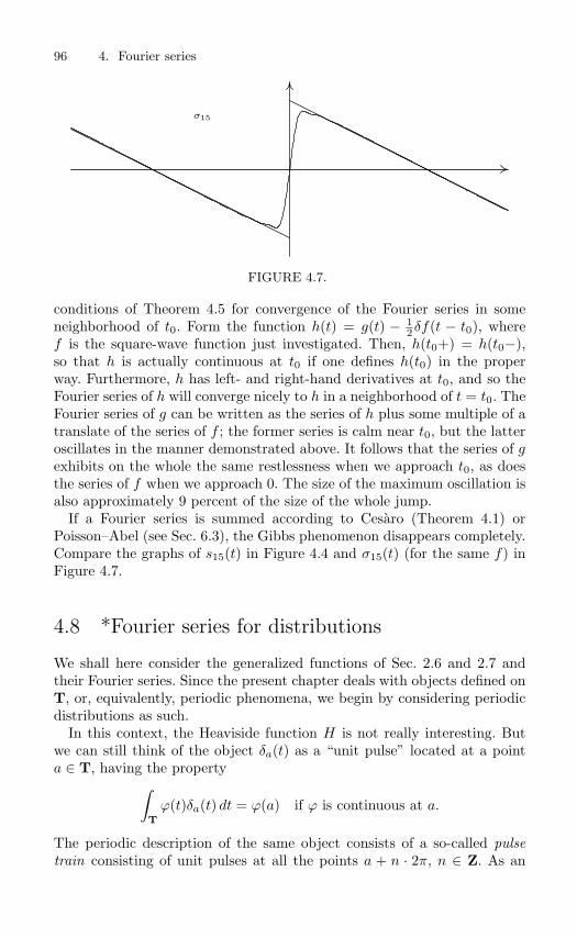
96 4. Fourier series
σ15
FIGURE 4.7.
conditions of Theorem 4.5 for convergence of the Fourier series in someneighborhood of t0. Form the function h(t) = g(t) − 1
2δf(t − t0), wheref is the square-wave function just investigated. Then, h(t0+) = h(t0−),so that h is actually continuous at t0 if one defines h(t0) in the properway. Furthermore, h has left- and right-hand derivatives at t0, and so theFourier series of h will converge nicely to h in a neighborhood of t = t0. TheFourier series of g can be written as the series of h plus some multiple of atranslate of the series of f ; the former series is calm near t0, but the latteroscillates in the manner demonstrated above. It follows that the series of gexhibits on the whole the same restlessness when we approach t0, as doesthe series of f when we approach 0. The size of the maximum oscillation isalso approximately 9 percent of the size of the whole jump.
If a Fourier series is summed according to Cesaro (Theorem 4.1) orPoisson–Abel (see Sec. 6.3), the Gibbs phenomenon disappears completely.Compare the graphs of s15(t) in Figure 4.4 and σ15(t) (for the same f) inFigure 4.7.
4.8 *Fourier series for distributions
We shall here consider the generalized functions of Sec. 2.6 and 2.7 andtheir Fourier series. Since the present chapter deals with objects defined onT, or, equivalently, periodic phenomena, we begin by considering periodicdistributions as such.
In this context, the Heaviside function H is not really interesting. Butwe can still think of the object δa(t) as a “unit pulse” located at a pointa ∈ T, having the property∫
Tϕ(t)δa(t) dt = ϕ(a) if ϕ is continuous at a.
The periodic description of the same object consists of a so-called pulsetrain consisting of unit pulses at all the points a + n · 2π, n ∈ Z. As an

4.8 *Fourier series for distributions 97
object defined on R, this pulse train could be described by
∞∑n=−∞
δa+2πn(t) =∞∑
n=−∞δ(t− a− 2πn).
The convergence of this series is uncontroversial, because at any individualpoint t at most one of the terms is different from zero.
The derivatives of δa can be described using integration by parts, just asin Sec. 2.6, but now the integrals are taken over T (i.e., over one period).Because everything is periodic, the contributions at the ends of the intervalwill cancel:∫
Tϕ(t)δ′
a(t) dt =[ϕ(t)δa(t)
]b+2π
b
−∫Tϕ′(t)δa(t) dt = −ϕ′(a).
What would be the Fourier series of these distributions? Let us firstconsider δa. The natural approach is to define Fourier coefficients by theformula
cn =12π
∫Tδa(t)e−int dt =
12π
· e−ina.
The series then looks like this:
δa(t) ∼ 12π
∑n∈Z
e−ina · eint.
In particular, when a = 0, the Fourier coefficients are all equal to 1/(2π),and the series is
δ(t) ∼ 12π
∑n∈Z
eint.
By pairing terms with the same values of |n|, we can formally rewrite thisas
δ(t) ∼ 12π
+1π
∞∑n=1
cosnt.
Compare the Dirichlet kernel! We might say that δ is the limit of DN asN → ∞.
These series cannot be convergent in the usual sense, since their terms donot tend to zero. But for certain values of t they can be summed accordingto Cesaro. Indeed, we can use the result of Exercise 2.16 on page 22. Theseries for 2πδa can be written (with z = ei(t−a))
∑n∈Z
ein(t−a) =∞∑
n=0
(ei(t−a)
)n
+−1∑
n=−∞
(ei(t−a)
)n
=∞∑
n=0
zn +∞∑
n=1
(e−i(t−a)
)n
=∞∑
n=0
zn + z
∞∑n=0
zn

98 4. Fourier series
According to Exercise 2.16, both the series in the last expression can besummed (C, 1) if |z| = 1 but z = 1, which is the case if t = a, and theresult will be
11 − z
+z
1 − z=
1 − z + z(1 − z)|1 − z|2 =
1 − zz
|1 − z|2 =1 − |z|2|1 − z|2 = 0.
If t = a, all the terms are ones, and the series diverges to infinity.Thus the series behaves in a way that is most satisfactory, as it enhances
our intuitive image of what δa looks like.Next we find the Fourier series of δ′
a. The coefficients are
cn =12π
∫ π
−π
δ′a(t)e−int dt = − 1
2π· d
dte−int
∣∣∣∣t=a
= − 12π
(−ine−int)∣∣t=a
=in
2πe−ina.
We recognize that the rule in Sec. 4.3 for the Fourier coefficients of a deriva-tive holds true. The summation of the series
δ′a(t) =
i
2π
∑n∈Z
ne−ianeint =i
2π
∑n∈Z
nein(t−a)
is tougher than that of δa itself, because the terms now have moduli thateven tend to infinity as |n| → ∞. It can be shown, however, that for t = athe series is summable (C, 2) to 0.
We give a couple of examples to illustrate the use of these series.
Example 4.8. Consider the function of Example 4.2 on page 78. ItsFourier series can be written
f(t) ∼∞∑
n=1
sinntn
=∑n =0
12in
eint.
(Notice that the last version is correct — the minus sign in the Eulerformula for sin is incorporated in the sign of the n in the coefficient.)
The derivative of f consists of an “ordinary” term − 12 , which takes care
of the slope between the jumps, and a pulse train that on T is identifiedwith π · δ(t). This would mean that the Fourier series of the derivative isgiven by
f ′(t) = − 12 + πδ(t) ∼ − 1
2 + π · 12π
∑n∈Z
eint
= − 12 + 1
2
∑n∈Z
eint = 12
∞∑n=1
(eint + e−int) =∞∑
n=1
cosnt.
Notice that this is precisely what a formal differentiation of the originalseries would yield.

4.8 *Fourier series for distributions 99
Example 4.9. Find a 2π-periodic solution of the differential equationy′ + y = 1 + δ(t) (−π < t < π).
Solution. We try a solution of the form y =∑cne
int. Differentiating thisand expanding the right-hand member in Fourier series, we get∑
n∈Z
incneint +
∑n∈Z
cneint = 1 +
∑n∈Z
12π
eint,
or
c0 +∑n =0
(in+ 1)cn eint =(
1 +12π
)+∑n =0
12π
eint.
Identification of coefficients yields c0 = 1 + 1/(2π) and, for n = 0, cn =1/(2π(1 + in)). A solution should thus be given by
y(t) ∼(
1 +12π
)+
12π
∑n =0
eint
1 + in.
By a stroke of luck, it happens that this series has been almost encounteredbefore in the text: in Example 4.1 on page 76 f. we found that
f(u) ∼ sinhππ
(1 +
∑n =0
(−1)n
1 − ineinu
),
where f(u) = eu for −π < u < π and f has period 2π. From this we canfind that ∑
n =0
(−1)n
1 − ineinu =
π
sinhπf(u) − 1.
On the other hand, the series on the left of this equation can be rewritten,using (−1)n = einπ and letting t = π − u:
∑n =0
(−1)n
1 − ineinu =
∑n =0
(−1)n
1 + ine−inu =
∑n =0
ein(π−u)
1 + in=∑n =0
eint
1 + in.
This means that our solution can be expressed in the following way:
y(t) ∼(
1+12π
)+
12π
(π
sinhπf(u)−1
)= 1+
12 sinhπ
f(u) = 1+f(π − t)2 sinhπ
.
In particular,
y(t) = 1 +eπ−t
2 sinhπ= 1 +
eπ
2 sinhπe−t, 0 < t < 2π,
since this condition on t is equivalent to −π < π − t < π. At the pointst = n · 2π, y(t) has an upward jump of size 1 (check this!).

100 4. Fourier series
Let us check the solution by substitution into the equation. Differenti-ating, we find that y′(t) contains the pulse δ(t) at the origin, and betweenjumps one has y′(t) = −(y(t) − 1). This proves that we have indeed founda solution.
Exercises
4.30 Let f be the even function with period 2π that satisfies f(t) = π − t for0 ≤ t ≤ π. Determine f ′ and f ′′, and use the result to find the Fourierseries of f .
4.31 Let f have period 2π and satisfy
f(t) =
et, |t| < π/2,
0, π/2 < |t| < π.
Compute f ′ − f , and then determine the Fourier series of f .
Summary of Chapter 4
DefinitionIf f is a sufficiently nice function defined on T, we define its Fourier coef-ficients by
cn =12π
∫Tf(t)e−int dt or
an
bn=
1π
∫Tf(t)
cossinnt dt.
The Fourier series of f is the series
∑n∈Z
cneint, resp. 1
2a0 +∞∑
n=1
(an cosnt+ bn sinnt).
If f has a period other than 2π, the formulae have to be adjusted accord-ingly. If f is even or odd, the formulae for an and bn can be simplified.TheoremIf two continuous functions f and g have the same Fourier coefficients, thenf = g.
TheoremIf f is piecewise continuous on T and continuous at the point t, then, forthis value of t, its Fourier series is summable (C, 1) to the value f(t).
TheoremIf f is continuous on T and its Fourier coefficients satisfy
∑ |cn| < ∞, thenits Fourier series converges absolutely and uniformly to f(t) on all of T.

Historical notes 101
TheoremIf f is differentiable on T, then the Fourier series of the derivative f ′ canbe found by termvise differentiation.
TheoremIf f ∈ Ck(T), then its Fourier coefficients satisfy |cn| ≤ M/|n|k.
TheoremIf f is continuous except for jump discontinuities, and if it has (generalized)one-sided derivatives at a point t, then its Fourier series for this value of tconverges with the sum 1
2 (f(t+) + f(t−)).Formulae for Fourier series are found on page 251.
Historical notes
Joseph Fourier was not the first person to consider trigonometric series ofthe kind that came to bear his name. Around 1750, both Daniel Bernoulli andLeonhard Euler were busy investigating these series, but the standard of rigor inmathematics then was not sufficient for a real understanding of them. Part of theproblem was the fact that the notion of a function had not been made precise,and different people had different opinions on this matter. For example, a graphpieced together as in Figure 4.2 on page 78 was not considered to represent onefunction but several. It was not until the times of Bernhard Riemann and Karl
Weierstrass that something similar to the modern concept of a function wasborn. In 1822, when Fourier’s great treatise appeared, it was generally regarded asabsurd that a series with terms that were smooth and nice trigonometric functionsshould be able to represent functions that were not everywhere differentiable, oreven worse—discontinuous!
The convergence theorem (Theorem 4.5) as stated in the text is a weakerversion of a result by the German mathematician J. Peter Lejeune-Dirichlet
(1805–59). At the age of 19, the Hungarian Lipot Fejer (1880–1959) had thebright idea of applying Cesaro summation to Fourier series.
In the twentieth century the really hard questions concerning the convergenceof Fourier series were finally resolved, when Lennart Carleson (1928–) provedhis famous Theorem 4.6. The author of this book, then a graduate student,attended the series of seminars in the fall of 1965 when Carleson step by stepconquered the obstacles in his way. The final proof consists of 23 packed pages inone of the world’s most famous mathematical journals, the Acta Mathematica.
Problems for Chapter 4
4.32 Determine the Fourier series of the following functions. Also state what isthe sum of the series for all t.(a) f(t) = 2 + 7 cos 3t− 4 sin 2t, −π < t < π.(b) f(t) = |sin t|, −π < t < π.

102 4. Fourier series
(c) f(t) = (π − t)(π + t), −π < t < π.(d) f(t) = e|t|, −π < t < π.
4.33 Find the cosine series of f(t) = sin t, 0 < t < π.4.34 Find the sine series of f(t) = cos t, 0 < t < π. Use this series to show that
π√
216
=1
22 − 1− 3
62 − 1+
5102 − 1
− 7142 − 1
+ · · · .
4.35 Let f be the 2π-periodic continuation of the function H(t− a) −H(t− b),where −π < a < b < π. Find the Fourier series of f . For what values of tdoes it converge? Indicate its sum for for all such t ∈ [−π, π].
4.36 Let f be given by f(x) = −1 for −1 < x < 0, f(x) = x for 0 ≤ x ≤ 1 andf(x + 2) = f(x) for all x. Compute the Fourier series of f . State the sumof this series for x = 10, x = 10.5, and x = 11.
4.37 Develop f(t) = t(t − 1), 0 < t < 1, period 1, in a Fourier series. Quotesome criterion that implies that the series converges to f(t) for all valuesof t.
4.38 The function f is defined by f(t) = t2 for 0 ≤ t ≤ 1, f(t) = 0 for 1 < t < 2and by the statement that it has period 2.(a) Develop f in a Fourier series with period 2 and indicate the sum of theseries in the interval [0, 5].
(b) Compute the value of the sum s =∞∑
n=1
(−1)n
n2 .
4.39 Suppose that f is integrable, has period T , and Fourier series
f(t) ∼∞∑
n=−∞cn e
2πint/T .
Determine the Fourier series of the so-called autocorrelation function r off , which is defined by
r(t) =1T
∫ T
0
f(t+ u) f(u) du.
4.40 An application to sound waves: Suppose the variation in pressure, p, thatcauses a sound has period 1
262 s (seconds), and satisfies
p(t) = 1, 0 < t < 11048 ,
p(t) = 78 ,
1524 < t < 3
1048 ,
p(t) = − 78 ,
11048 < t < 1
524 ,
p(t) = −1, 31048 < t < 1
262 .
What frequencies can be heard in this sound? Which is the dominant fre-quency?
4.41 Compute the Fourier series of f , given by
f(x) =∣∣∣sin x2 ∣∣∣ , −π < x ≤ π; f(x+ 2π) = f(x), x ∈ R.
Then find the values of the sums
s1 =∞∑
n=1
14n2 − 1
and s2 =∞∑
n=1
(−1)n
4n2 − 1.

Problems for Chapter 4 103
4.42 Let f be an even function of period 2π described by f(x) = cos 2x for0 ≤ x ≤ 1
2π and f(x) = −1 for 12π < x ≤ π. Find its Fourier series and
compute the value of the sum
s =∞∑
k=1
(−1)k
(2k + 1)(2k − 1)(2k + 3).
4.43 Find all solutions y(t) with period 2π of the differential-difference equation
y′(t) + y(t− 12π) − y(t− π) = cos t, −∞ < t < ∞.
4.44 Let f be an even function with period 4 such that f(x) = 1−x for 0 ≤ x ≤ 1and f(x) = 0 for 1 < x ≤ 2. Find its Fourier series and compute
s =∞∑
k=0
1(2k + 1)2
.
4.45 Let α be a real number but not an integer. Define f(x) by putting f(x) =eiαx for −π < x < π and f(x+ 2π) = f(x). By studying its Fourier series,prove the following formulae:
π
sinπα=
1α
+∞∑
n=1
2(−1)nα
α2 − n2 .
(π
sinπα
)2
=∞∑
n=−∞
1(α− n)2
.
4.46 Compute the Fourier series of the 2π-periodic function f given by f(x) =x3 − π2x for −π < x < π. Find the sum
s =∞∑
n=1
(−1)n+1
(2n− 1)3.
4.47 Let f be a 2π-periodic function with (“complex”) Fourier coefficients cn
(n ∈ Z). Assume that for an integer k > 0 it holds that∑n∈Z
|n|k |cn| < ∞.
Prove that f is of class Ck, i.e., that the kth derivative of f is continuous.
4.48 Find the Fourier series of f with period 2 which is given for |x| < 1 byf(x) = 2x2 − x4. The result can be used to find the value of the sum
ζ(4) =∞∑
n=1
1n4 .

This page intentionally left blank

5L2 Theory
5.1 Linear spaces over the complex numbers
We assume that the reader is familiar with vector spaces, where the scalarsare real numbers. It is also possible, and indeed very fruitful, to allow scalarsto be complex numbers. Thus, we consider now a set V , whose elements canbe added to each other, and also can be multiplied by complex numbers,to produce new elements in V ; and these operations are to obey the samerules of calculation as in ordinary real vector spaces. Simple examples ofsuch complex vector spaces are given by Cn, which consists of n-tuplesz = (z1, z2, . . . , zn) of complex numbers. Another example is the set of allcomplex-valued functions f defined on an interval [a, b].
It turns out that elementary complex linear algebra can be developed inalmost exact parallel to its real counterpart. Linear dependence, subspaces,and dimension can be defined word for word in the same way, with the un-derstanding that all scalars occurring in the process are complex numbers.This gives a new significance to the notion of dimension. For example, Cis a one-dimensional complex vector space. It could also be considered asa real vector space, but then the dimension is 2. In the same manner, Cn
has complex dimension n but real dimension 2n.When we reach the notions of scalar product and distance, we must,
however, modify the details. The old formula for the (standard) scalarproduct of two vectors z and w in n-space has the form 〈z,w〉 = z1w1 +z2w2 + · · · + znwn. This cannot be allowed to hold any more, because itdoes not work in a reasonable way.
106 5. L2 Theory
Example 5.1. Consider the vector z = (1, i) ∈ C 2. With the usualformula for the scalar product we would get |z|2 = 1 · 1 + i · i = 1 − 1 = 0.The length of the vector would be 0, which is no good. Still more strangewould be the case for the vector w = (1, 2i), which would not even havereal length.
By considering the one-dimensional space C, we can get an idea for amore suitable definition. The vector, or number, z = x+iy is normally iden-tified with the vector (x, y) in R2. The length of this vector is the number|z| =
√x2 + y2 =
√zz. If the scalar product of two complex numbers z
and w is defined to be 〈z, w〉 = zw, we get the formula |z|2 = 〈z, z〉. Thismeans that we have to modify a few rules for the scalar product, but thatprice is well worth paying. Just to indicate that the rules of computationare no longer exactly the same, we choose to use the name inner productinstead of scalar product.
Definition 5.1 Let V be a complex vector space. An inner product on Vis a complex-valued function 〈u, v〉 of u and v ∈ V having the followingproperties:
(1) 〈u, v〉 = 〈v, u〉 (Hermitian symmetry)(2) 〈αu+ βv,w〉 = α〈u,w〉 + β〈v, w〉 (Linearity in the first argument)(3) 〈u, u〉 ≥ 0(4) 〈u, u〉 = 0 ⇒ u = 0
(Positive-definiteness)
Combining rules 1 and 2 we find the rule
(5) 〈u, αv + βw〉 = α〈u, v〉 + β〈u,w〉.
Example 5.2. In Cn, we can define an inner product (using naturalnotation) by the formula
〈z,w〉 = z1w1 + z2w2 + · · · + znwn.
Example 5.3. Let C(a, b) be the set of continuous, complex-valued func-tions defined on the compact interval [a, b], and put
〈f, g〉 =∫ b
a
f(x) g(x) dx.
The fact that this is an inner product is almost trivial, except possiblyfor condition 4. That implication follows from the fact that if a continu-ous function is non-negative on an interval and its integral is 0, then thefunction must indeed be identically 0 (see textbooks on calculus).

5.1 Linear spaces over the complex numbers 107
Example 5.4. More generally, let w be a fixed continuous function on[a, b] such that w(x) > 0, and put
〈f, g〉 =∫ b
a
f(x) g(x)w(x) dx.
A complex vector space with a chosen inner product is called an inner
product space. Because of rules 3 and 4 it is natural to define a measure ofthe size of a vector in such a space, corresponding to the length in the realcase. One prefers to use the word norm instead of length and write
the norm of u = ‖u‖ =√
〈u, u〉.
In the case described in Example 5.3 we thus have
‖f‖2 =∫ b
a
|f(x)|2 dx.
The following inequalities are wellknown in the real case, and they holdjust as well in the new setting:
Theorem 5.1
|〈u, v〉| ≤ ‖u‖ ‖v‖ (Cauchy–Schwarz inequality)‖u+ v‖ ≤ ‖u‖ + ‖v‖ (Triangle inequality)
Proof. (a) If u = 0, then both members are 0 and the statement is true.Thus, let us assume that u = 0. Put α = −〈v, u〉/〈u, u〉. Then,
0 ≤ ‖αu+ v‖2 = 〈αu+ v, αu+ v〉 = αα〈u, u〉 + α〈u, v〉 + α〈v, u〉 + 〈v, v〉=
〈v, u〉 · 〈u, v〉〈u, u〉2 〈u, u〉 − 〈v, u〉
〈u, u〉 〈u, v〉 − 〈u, v〉〈u, u〉 〈v, u〉 + 〈v, v〉
= −|〈u, v〉|2〈u, u〉 + 〈v, v〉.
Rearranging this we arrive at the Cauchy–Schwarz inequality.(b) The triangle inequality is proved using Cauchy–Schwarz:
‖u+ v‖2 = 〈u+ v, u+ v〉 = ‖u‖2 + 〈u, v〉 + 〈v, u〉 + ‖v‖2
= ‖u‖2 + 2 Re 〈u, v〉 + ‖v‖2 ≤ ‖u‖2 + 2|〈u, v〉| + ‖v‖2
≤ ‖u‖2 + 2‖u‖ ‖v‖ + ‖v‖2 =(‖u‖ + ‖v‖)2.
Since both ‖u + v‖ and ‖u‖ + ‖v‖ are non-negative numbers, the triangleinequality follows.

108 5. L2 Theory
Two vectors u and v are called orthogonal with respect to the choseninner product, if 〈u, v〉 = 0. A vector u is normed if ‖u‖ = 1; and anorthonormal , or simply ON, set of vectors consists of normed and pairwiseorthogonal vectors.
Example 5.5. C(T) consists of the continuous complex-valued functionson the unit circle T, and let the inner product be defined by
〈f, g〉 =12π
∫Tf(x) g(x) dx.
Let ϕk(x) = eikx, k ∈ Z. Then we have
〈ϕm, ϕn〉 =12π
∫Teimx e−inx dx =
12π
∫ π
−π
ei(m−n)x dx =
0, m = n1, m = n
The sequence ϕk∞k=−∞ is thus an orthonormal set in C(T).
Just as in the case of real spaces one can show that a set of non-zero,pairwise orthogonal vectors is linearly independent. In a space with finite(complex) dimension N , an orthonormal set can thus contain at most Nvectors. On the other hand, there always exists such a set. Starting froman arbitrary basis in the space, one can use the Gram–Schmidt process toconstruct an ON basis, working precisely as in the real case.
Example 5.6. As a reminder of the Gram–Schmidt process, we construct anorthonormal basis in the space of polynomials of degree at most 2, with the innerproduct
〈f, g〉 =∫ 1
0
f(x)g(x)(1 + x) dx.
The “raw material” consists of the vectors u0, u1, u2 defined by
u0(x) = 1, u1(x) = x, u2(x) = x2.
As a tentative first vector in the new basis we choose v0 = u0, which is to beadjusted to have unit norm. Since
‖v0‖2 = 〈v0, v0〉 =∫ 1
0
1 · 1 · (1 + x) dx = 32 ,
the normed vector is described by
ϕ0(x) =v0(x)‖v0‖ =
√23 .
Next we adjust u1 so that it is orthogonal to ϕ0. This is done by subtracting acertain multiple of ϕ0 according to the following recipe:
v1 = u1 − 〈u1, ϕ0〉ϕ0.
The inner product is
〈u1, ϕ0〉 =∫ 1
0
x ·√
23 (1 + x) dx = 5
6
√23 .
5.1 Linear spaces over the complex numbers 109
Thus,
v1(x) = x− 56
√23 ·√
23 = x− 5
9 .
The squared norm of v1 is
‖v1‖2 = 〈v1, v1〉 =∫ 1
0
(x− 5
9
)2(x+ 1) dx = 13
108 .
Thus the second normed basis vector is
ϕ1(x) =x− 5
9√13108
= 6√
313
(x− 5
9 ).
The third vector is obtained by the following steps:
v2 = u2 − 〈u2, ϕ0〉ϕ0 − 〈u2, ϕ1〉ϕ1, 〈u2, ϕ0〉 = 736
√6, 〈u2, ϕ1〉 = 34
585
√39,
v2 = x2 − 6865 x+ 5
26 , 〈v2, v2〉 = 212600 ,
ϕ2 = 1021
√546
(x2 − 68
65 x+ 526
).
It is obvious that the computations quickly grow very involved, not least be-cause the norms turn out to be rather hideous numbers. Mostly, therefore, one issatisfied with just orthogonal sets, instead of orthonormal sets.
There is also the following theorem, which should be proved by thereader:
Theorem 5.2 If ϕ1, ϕ2, . . . , ϕN is an ON basis in an N -dimensional inner
product space V , then every u ∈ V can be written as u =N∑
j=1〈u, ϕj〉ϕj, and
furthermore one has
‖u‖2 =N∑
j=1
|〈u, ϕj〉|2 (theorem of Pythagoras).
For the inner product of two vectors one also has the following formula:
〈u, v〉 =N∑
j=1
〈u, ϕj〉〈v, ϕj〉.
Exercises5.1 Let u = (1 − 2i, 3, 2 + i) and v = (i, 1 − 3i, 0) be vectors in C 3. Compute
‖u‖, ‖v‖, and 〈u,v〉.5.2 Let C(−1, 1) be as in Example 5.3 above, and let f and g ∈ C(−1, 1) be
described by f(x) = x+ 2, g(x) = ix+ x2. Compute 〈f, g〉.5.3 Are the functions 1, x, x2, . . . , xn, sinx, cosx, ex linearly independent,
considered as vectors in C(0, 1) ? (n is some positive integer.)

110 5. L2 Theory
5.4 Apply the Gram–Schmidt orthogonalization procedure to construct an or-thogonal basis in the subspace of C(0, 1) spanned by the polynomials 1, xand x2.
5.5 Orthogonalize the following sets of vectors:(a) the vectors (1, 2, 3), (3, 1, 4) and (2, 1, 1) in C 3;(b) the functions 1, x, x2 i C(−1, 1);(c) the functions e−x, xe−x, x2e−x in C(0,∞).
5.6 Prove the following formula for the inner product:
4〈u, v〉 = ‖u+ v‖2 + i‖u+ iv‖2 − ‖u− v‖2 − i‖u− iv‖2.
5.2 Orthogonal projections
The reader should recall the following fact from real linear algebra: LetϕkN
k=1 be an orthonormal set in the space V , and let u be an arbitraryvector in V . The orthogonal projection of u on to the subspace of V spannedby ϕkN
k=1 is the vector
PN (u) = 〈u, ϕ1〉ϕ1 + 〈u, ϕ2〉ϕ2 + · · · + 〈u, ϕN 〉ϕN =N∑
k=1
〈u, ϕk〉ϕk.
This definition works just as well in the complex case, and the projectionthus defined has also the least-squares property described in the followingtheorem.
Theorem 5.3 (Least squares approximation) Let ϕkNk=1 be an or-
thonormal set in an inner product space V and let u be a vector in V .Among all the linear combinations Φ =
∑Nk=1 γkϕk, the one that minimizes
the value of ‖u−Φ‖ is the one with the coefficients γk equal to 〈u, ϕk〉, i.e.,Φ = PN (u).
Proof. For brevity, we write 〈u, ϕk〉 = ck. We get
‖u− Φ‖2 = 〈u− Φ, u− Φ〉 =
⟨u−
N∑k=1
γkϕk, u−N∑
k=1
γkϕk
⟩
= 〈u, u〉 −⟨u,
N∑k=1
γkϕk
⟩−⟨
N∑k=1
γkϕk, u
⟩+
⟨N∑
k=1
γkϕk,
N∑k=1
γkϕk
⟩
= 〈u, u〉 −N∑
k=1
γk〈u, ϕk〉 −N∑
k=1
γk〈ϕk, u〉 +N∑
k=1
N∑j=1
γkγj〈ϕk, ϕj〉
= 〈u, u〉 −N∑
k=1
(γkck + γkck) +N∑
k=1
γkγk

5.2 Orthogonal projections 111
= ‖u‖2 +N∑
k=1
(γkγk − γkck − γkck + ckck) −N∑
k=1
|ck|2
= ‖u‖2 +N∑
k=1
|γk − ck|2 −N∑
k=1
|ck|2.
In the last expression, we note that u is given in the formulation of thetheorem; also, since the ϕk are given, the ck = 〈u, ϕk〉 are given. But wehave the γk at our disposal, to minimize the value of the expression. Inorder to make it as small as possible, we choose the numbers γk to be equalto ck, which proves the assertion.
A couple of consequences of the proof are worth emphasizing. When avector u is approximated by the orthogonal projection PN (u), then the“error” u − PN (u) is called the residual. An important fact is that theresidual is orthogonal to the projection. As for the “size” of the residual,we have the identity (“Pythagoras’ theorem”)
‖u− PN (u)‖2 = ‖u‖2 − ‖PN (u)‖2.
If this is written out in full, it becomes
∥∥∥u−N∑
k=1
〈u, ϕk〉ϕk
∥∥∥2= ‖u‖2 −
N∑k=1
|〈u, ϕk〉|2. (5.1)
Since the left-hand member of these equations is non-negative, we also have
‖PN (u)‖2 ≤ ‖u‖2, or ‖PN (u)‖ ≤ ‖u‖,
or, indeed,N∑
k=1
|〈u, ϕk〉|2 ≤ ‖u‖2.
If the ON set contains infinitely many vectors, we can let N → ∞ and getwhat is known as the Bessel inequality:
∞∑k=1
|〈u, ϕk〉|2 ≤ ‖u‖2.
Let us now concentrate on the case when the space V has infinite dimen-sion. A system ϕj∞
j=1 in V is said to be complete in V if, for every u ∈ V
and every ε > 0, there exists a linear combination∑N
j=1 ajϕj such that∥∥∥∥∥∥u−N∑
j=1
ajϕj
∥∥∥∥∥∥ < ε.

112 5. L2 Theory
This means that every u in V can be approximated arbitrarily closely, in thesense of the norm, by linear combinations of the elements in the set ϕj.The theorem above shows that the best approximation must be given bythe “infinite projection”
∑∞j=1〈u, ϕj〉ϕj of u. A condition that is equivalent
to completeness is given by the following theorem:
Theorem 5.4 The ON system ϕj∞j=1 is complete in V if and only if for
every u ∈ V it holds that
‖u‖2 =∞∑
j=1
|〈u, ϕj〉|2
(the Parseval formula or the completeness relation).
The proof follows from (5.1).As a corollary we also have the following:
Theorem 5.5 (Expansion theorem) If the ON system ϕj∞j=1 is com-
plete in V , then every u ∈ V can be written as u =∑∞
j=1〈u, ϕj〉ϕj, where
the series converges in the sense of the norm (i.e.,∥∥∥u−∑N
j=1〈u, ϕj〉ϕj
∥∥∥ →0 as N → ∞).
Furthermore, one has the following theorem, which generalizes the usualformula (in finite dimension) for computing the inner product in an ONbasis:
Theorem 5.6 If the ON system ϕj∞j=1 is complete in V , then
〈u, v〉 =∞∑
j=1
〈u, ϕj〉〈v, ϕj〉
for all u, v ∈ V .
Proof. Let Pn(u) be the projection of u on to the subspace spanned by then first ϕ’s:
Pn(u) =n∑
j=1
〈u, ϕj〉ϕj .
By Theorem 5.2 we have
〈Pn(u), Pn(v)〉 =n∑
j=1
〈u, ϕj〉〈v, ϕj〉.
Using the triangle and Cauchy–Schwarz inequalities, we get
|〈u, v〉 − 〈Pn(u), Pn(v)〉|

5.2 Orthogonal projections 113
= |〈u, v〉 − 〈u, Pn(v)〉 + 〈u, Pn(v)〉 − 〈Pn(u), Pn(v)〉|≤ |〈u, v − Pn(v)〉| + |〈u− Pn(u), Pn(v)〉|≤ ‖u‖ ‖v − Pn(v)‖ + ‖u− Pn(u)‖ ‖Pn(v)‖≤ ‖u‖ ‖v − Pn(v)‖ + ‖u− Pn(u)‖ ‖v‖.
In the last part we also used Bessel’s inequality. Now we know, because ofcompleteness, that ‖v − Pn(v)‖ → 0 as n → ∞, and similarly for u, whichimplies that the final member of the estimate tends to zero. Then also thefirst member must tend to zero, and so
〈u, v〉 = limn→∞〈Pn(u), Pn(v)〉 =
∞∑j=1
〈u, ϕj〉〈v, ϕj〉,
and the proof is complete. Remark. Using an estimate of the same kind as in the proof, one can see that〈u, v〉 is a continuous function of u and v in the sense that if un → u and vn → v(in the sense of the norm), then 〈un, vn〉 → 〈u, v〉.
In the interest of simplicity, we have throughout this section been workingwith orthonormal systems. In practice one is often satisfied with usingorthogonal systems, since the normalizing factors can be quite unwieldynumbers. In such a case, our formulae have to be somewhat modified.
The projection of u on to an orthogonal set of vectors ϕjNj=1 is given
by
PN (u) =N∑
j=1
〈u, ϕj〉〈ϕj , ϕj〉 ϕj =
N∑j=1
〈u, ϕj〉‖ϕj‖2 ϕj .
The other formulae must be adjusted in the same vein: every ϕj that occurshas to be divided by its norm, and this holds whether ϕj is “free” or is partof an inner product. For example, the Parseval formula takes the form
‖u‖2 =∞∑
j=1
|〈u, ϕj〉|2‖ϕj‖2 ,
and the formula for inner products is
〈u, v〉 =∞∑
j=1
〈u, ϕj〉〈v, ϕj〉‖ϕj‖2 .
Exercises5.7 Determine the polynomial p of degree at most 1 that minimizes∫ 2
0|ex −p(x)|2 dx. (Hint: first find an orthogonal basis for a suitably chosen
space of polynomials of degree ≤ 1.)
114 5. L2 Theory
5.8 Determine the constants a and b in order to minimize the integral∫ 1
−1|ax+ bx2 − sinπx|2 dx.
5.9 Find the polynomial p(x) of degree at most 2 that minimizes the integral∫ π/2
−π/2
| sinx− p(x)|2 cosx dx.
5.3 Some examples
We have already seen the finite-dimensional inner-product spaces Cn. Ageneralization of these spaces can be constructed in the following manner.Let M be an arbitrary set (with finitely or infinitely many elements). Letl2(M) be the set of all functions a : M → C such that∑
x∈M
|a(x)|2 < ∞. (5.2)
The fact that this defines a linear space can be proved in the following way.Because of the inequality
|pq| ≤ 12 (|p|2 + |q|2), (5.3)
that holds for all complex numbers p and q, the following estimate is true:
|λa+ µb|2 = (λa+ µb)(λa+ µb) = |λ|2|a|2 + |µ|2|b|2 + 2Re λµab≤ |λ|2|a|2 + |µ|2|b|2 + 2|λa||µb| ≤ 2
(|λ|2|a|2 + |µ|2|b|2).Using this, and the comparison test for positive series, one finds that if∑ |a(x)|2 and
∑ |b(x)|2 are both convergent, then∑ |λa(x) + µb(x)|2 is
also convergent. This means that linear combinations of elements in l2(M)also belong to l2(M). Using (5.3) we also see that if both a and b aremembers of l2(M), then the series∑
x∈M
a(x) b(x)
will converge absolutely. This expression can be taken as the definition ofan inner product 〈a, b〉. The square of the norm of a is then given by theleft member of (5.2).
If, as an example, we choose M = N = 0, 1, 2, . . ., we can write an
instead of a(n) and get the inner product∑∞
n=0 an bn. This certainly lookslike a natural generalization of Cn.
When we gave examples of inner products in function spaces in Sec. 5.1,we assumed, for convenience, that all the functions were continuous. It is,however, often desirable to be able to work with more general functions.

5.3 Some examples 115
One such class is the class of Riemann-integrable functions, which consistsof functions that can be approximated in a certain way by so-called stepfunctions; the class includes, for example, functions with a finite number ofjumps. In order to get a really efficient theory, one should actually go stillfurther and allow measurable functions in the sense of Lebesgue. However,this is a rather complicated step, and in this text we shall confine ourselvesto more “ordinary” functions. At one point (p. 121), we shall, however,mention how the Lebesgue functions obtrude upon us.
In what follows, it will often be of no interest whether an interval containsits endpoints or not. For simplicity, we shall write (a, b), which can beinterpreted at will to mean either [a, b] or [a, b[, etc.
Let I be an interval, bounded or unbounded, and let w : I → ]0,∞[ be apositive, continuous, real-valued function on I. Let finally p be a number≥ 1. The set Lp(I, w) is defined to consist of all (Lebesgue-measurable)functions f such that ∫
I
|f(x)|p w(x) dx < ∞.
(The integral may be improper in one way or another, without this beingindicated when we write it.) It can be proved that this defines a linearspace: if f and g belong to it, then the same goes for all linear combinationsαf + βg. The proof is very simple in the case p = 1:∫
I
|αf + βg|w dx ≤ |α|∫
I
|f |w dx+ |β|∫
I
|g|w dx.
For p = 2, it can be done in a way that is analogous to what was donefor l2(M) above (integrals replacing sums). For other values of p it is moredifficult, and we skip it here.
The space Lp(I, w) is called the Lebesgue space with weight function wand exponent p. If the weight is identically 1 on all of I, one simply writesLp(I). For f ∈ Lp(I, w) one can define a norm
‖f‖p,w =(∫
I
|f(x)|p w(x) dx)1/p
,
that can be used to introduce a notion of distance ‖f − g‖p,w between twofunctions f and g. This, in turn, gives rise to a notion of convergence: we saythat a sequence of functions fn converges to g in Lp(I, w) if ‖fn−g‖p,w → 0as n → ∞.
In order for this to make sense, it is necessary to modify slightly what ismeant by equality between functions. Two functions f and g are consideredto be equal if their mutual distance is zero; explicitly this means that∫
I
|f(x) − g(x)|p w(x) dx = 0.

116 5. L2 Theory
This does not necessarily imply that f(x) = g(x) for all x, it means onlythat they are equal “almost everywhere”: the set where they differ is aso-called zero set (see the text preceding Theorem 4.6 on page 89). Whenworking with “nice” functions, which are continuous except for a finitenumber of jumps, this means that the function values are actually equalexcept possibly for at a finite number of points.
We shall almost exclusively consider the case p = 2. It can be provedthat only in this case can there exist an inner product 〈f, g〉 in Lp(I, w)such that the norm is recovered through the formula ‖f‖2 = 〈f, f〉. Thisinner product must be defined by
〈f, g〉 =∫
I
f(x) g(x)w(x) dx.
Let us now look at a few important cases.
Example 5.7. Let I = (−π, π) or, equivalently, interpret I as the unitcircle T, and take w(x) = 1. The inner product here is almost the same as inExample 5.5, page 108. There we showed that the functions ϕn(x) = einx
are orthogonal in C(T), and this holds equally well in L2(T). Becausethe factor 1/(2π) is now missing in the inner product, they are no longernormed, however, but the norm of each ϕn is now
√2π.
The formula for projections on to an orthogonal set of vectors has theform
PN (f) =N∑
n=1
〈f, ϕn〉〈ϕn, ϕn〉 ϕn =
N∑n=1
〈f, ϕn〉‖ϕn‖2 ϕn =
N∑n=1
cnϕn,
where
cn =〈f, ϕn〉‖ϕn‖2 =
12π
∫Tf(x) einx dx =
12π
∫Tf(x) e−inx dx.
We recognize our good old Fourier coefficients. Example 5.8. In the same space as in the preceding example we study thesystem consisting of firstly all the functions ϕn(x) = cosnx, n = 0, 1, 2, . . .,secondly all the functions ψn(x) = sinnx, n = 1, 2, 3, . . .. Using some suit-able trigonometric formula (or Euler’s formulae), it is easily proved that allthese functions are mutually orthogonal, and furthermore 〈ϕ0, ϕ0〉 = 2π,while all the other members of the system have the square of the normequal to π. Here, too, the coefficients in the orthogonal projections turnout to be the well-known classical Fourier coefficients. Example 5.9. In the space L2(0, π), the functions ϕn(x) = cosnx,n = 0, 1, 2, . . . form an orthogonal set, and ψn(x) = sinnx, n = 1, 2, 3, . . .another orthogonal set (check it!). However, as a rule, a ϕm is not orthog-onal to a ψn.

5.3 Some examples 117
Examples 5.7 and 5.8 provide a new viewpoint for considering Fourierseries. Such series can be regarded as representations with respect to anorthogonal system. The general results in Sections 5.1–2 concerning suchrepresentations are thus valid for our Fourier expansions. As an example,we formulate what Theorem 5.3 purports in the case of “real” Fourier series.
Theorem 5.7 Let f ∈ L2(T) and let N be a fixed non-negative integer.Among all trigonometric polynomials of the form
PN (x) = 12α0 +
N∑n=1
(αn cosnx+ βn sinnx),
the polynomial that minimizes the value of the integral∫T
|f(x) − PN (x)|2 dx
is the one where the coefficients are the usual Fourier coefficients of f , viz.,(using the ordinary notation) where αn = an and βn = bn.
We have also, for example, Bessel’s inequality, which can be written, incomplex and real guise, respectively, as
∑n∈Z
|cn|2 ≤ 12π
∫T
|f(x)|2 dx, 12 |a0|2+
∞∑n=1
(|an|2+|bn|2) ≤ 1π
∫T
|f(x)|2 dx.
The question of completeness will be addressed in the next section.
Remark. At this point, the reader will have been confronted by a number ofdifferent notions of convergence for sequences of functions. There is pointwiseconvergence and uniform convergence, and now we have also various versions ofLp convergence. It is natural to ask whether there are any sensible connectionsbetween all these notions.
It is trivial that uniform convergence implies pointwise convergence. If oneworks on a finite interval (a, b) with weight 1, it is also easy to see that uni-form convergence implies convergence in Lp(a, b). Indeed, suppose that fn → funiformly on (a, b). Then (p ≥ 1)
‖fn − f‖p =
(∫ b
a
|fn(t) − f(t)|p dt)1/p
≤(∫ b
a
sup(a,b)
|fn(t) − f(t)|p dt)1/p
= sup(a,b)
|fn(t) − f(t)|(∫ b
a
dt
)1/p
= C sup(a,b)
|fn(t) − f(t)| → 0
as n → ∞.In the converse direction, Lp convergence does not even imply pointwise con-
vergence. This is shown by the following example; for simplicity it is formulatedin L1(0, 1), but the same functions can be used to prove the same thing in allLp(0, 1), and they are easily rescaled to suit other intervals.
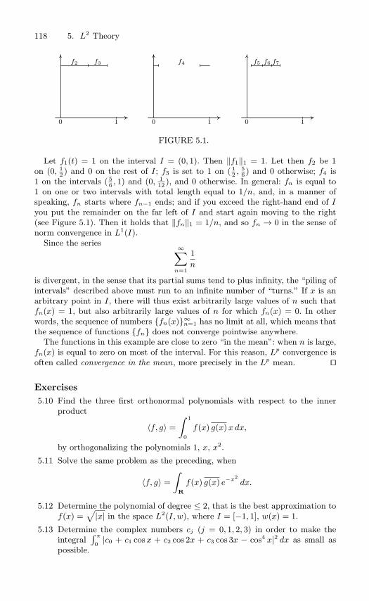
118 5. L2 Theory
0 1
f2 f3
0 1
f4
0 1
f5 f6 f7
FIGURE 5.1.
Let f1(t) = 1 on the interval I = (0, 1). Then ‖f1‖1 = 1. Let then f2 be 1on (0, 1
2 ) and 0 on the rest of I; f3 is set to 1 on ( 12 ,
56 ) and 0 otherwise; f4 is
1 on the intervals ( 56 , 1) and (0, 1
12 ), and 0 otherwise. In general: fn is equal to1 on one or two intervals with total length equal to 1/n, and, in a manner ofspeaking, fn starts where fn−1 ends; and if you exceed the right-hand end of Iyou put the remainder on the far left of I and start again moving to the right(see Figure 5.1). Then it holds that ‖fn‖1 = 1/n, and so fn → 0 in the sense ofnorm convergence in L1(I).
Since the series ∞∑n=1
1n
is divergent, in the sense that its partial sums tend to plus infinity, the “piling ofintervals” described above must run to an infinite number of “turns.” If x is anarbitrary point in I, there will thus exist arbitrarily large values of n such thatfn(x) = 1, but also arbitrarily large values of n for which fn(x) = 0. In otherwords, the sequence of numbers fn(x)∞
n=1 has no limit at all, which means thatthe sequence of functions fn does not converge pointwise anywhere.
The functions in this example are close to zero “in the mean”: when n is large,fn(x) is equal to zero on most of the interval. For this reason, Lp convergence isoften called convergence in the mean, more precisely in the Lp mean.
Exercises5.10 Find the three first orthonormal polynomials with respect to the inner
product
〈f, g〉 =∫ 1
0
f(x) g(x)x dx,
by orthogonalizing the polynomials 1, x, x2.
5.11 Solve the same problem as the preceding, when
〈f, g〉 =∫R
f(x) g(x) e−x2dx.
5.12 Determine the polynomial of degree ≤ 2, that is the best approximation tof(x) =
√|x| in the space L2(I, w), where I = [−1, 1], w(x) = 1.
5.13 Determine the complex numbers cj (j = 0, 1, 2, 3) in order to make theintegral
∫ π
0|c0 + c1 cosx + c2 cos 2x + c3 cos 3x − cos4 x|2 dx as small as
possible.
5.4 The Fourier system is complete 119
h
g
g
FIGURE 5.2.
5.4 The Fourier system is complete
We are now prepared to prove the following result, which, in a way, crownsthe classical Fourier theory.
Theorem 5.8 The two orthogonal systems eintn∈Z and cosnt, n ≥0; sinnt, n ≥ 1 are each complete in L2(T).
Proof. We want to prove that if f ∈ L2(T), then f can be approximatedarbitrarily well by linear combinations of elements from one of the systems.Since the elements of one system are simple linear combinations of elementsfrom the other system, it does not matter which of the systems we consider.Our proof will be incomplete in one way: we only show that functions fthat happen to be piecewise continuous can be approximated; but this isreally just due to the fact that we have not said anything about what amore general f might look like.
Thus we assume that f is piecewise continuous. It is then bounded on T,so that |f(t)| ≤ M for some constant M and all t. Now let ε > 0 be given.By the definition of the Riemann integral, there exists a step function (i.e.,a piecewise constant function) g such that∫
T|f(t) − g(t)| dt < ε2
2M.
Clearly we can choose g in such a way that |g(t)| ≤ M , and then it followsthat
‖f − g‖2 =∫T
|f(t) − g(t)|2 dt ≤∫T
2M |f(t) − g(t)| dt ≤ 2M · ε2
2M= ε2,
and so ‖f − g‖ < ε.In the next step of the proof we round off the corners of the step function
g to obtain a C2 function h such that ‖g − h‖ < ε. At this point, the
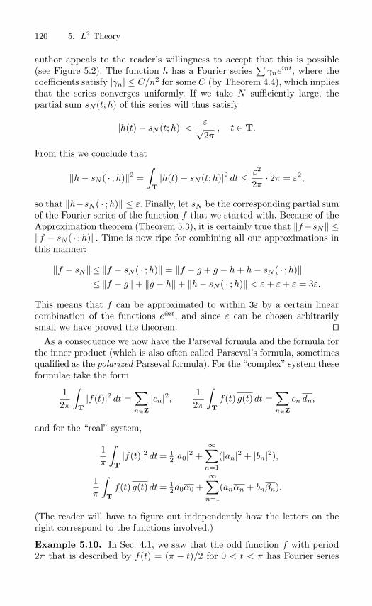
120 5. L2 Theory
author appeals to the reader’s willingness to accept that this is possible(see Figure 5.2). The function h has a Fourier series
∑γne
int, where thecoefficients satisfy |γn| ≤ C/n2 for some C (by Theorem 4.4), which impliesthat the series converges uniformly. If we take N sufficiently large, thepartial sum sN (t;h) of this series will thus satisfy
|h(t) − sN (t;h)| < ε√2π
, t ∈ T.
From this we conclude that
‖h− sN ( · ;h)‖2 =∫T
|h(t) − sN (t;h)|2 dt ≤ ε2
2π· 2π = ε2,
so that ‖h−sN ( · ;h)‖ ≤ ε. Finally, let sN be the corresponding partial sumof the Fourier series of the function f that we started with. Because of theApproximation theorem (Theorem 5.3), it is certainly true that ‖f−sN‖ ≤‖f − sN ( · ;h)‖. Time is now ripe for combining all our approximations inthis manner:
‖f − sN‖ ≤ ‖f − sN ( · ;h)‖ = ‖f − g + g − h+ h− sN ( · ;h)‖≤ ‖f − g‖ + ‖g − h‖ + ‖h− sN ( · ;h)‖ < ε+ ε+ ε = 3ε.
This means that f can be approximated to within 3ε by a certain linearcombination of the functions eint, and since ε can be chosen arbitrarilysmall we have proved the theorem.
As a consequence we now have the Parseval formula and the formula forthe inner product (which is also often called Parseval’s formula, sometimesqualified as the polarized Parseval formula). For the “complex” system theseformulae take the form
12π
∫T
|f(t)|2 dt =∑n∈Z
|cn|2, 12π
∫Tf(t) g(t) dt =
∑n∈Z
cn dn,
and for the “real” system,
1π
∫T
|f(t)|2 dt= 12 |a0|2 +
∞∑n=1
(|an|2 + |bn|2),
1π
∫Tf(t) g(t) dt= 1
2a0α0 +∞∑
n=1
(anαn + bnβn).
(The reader will have to figure out independently how the letters on theright correspond to the functions involved.)
Example 5.10. In Sec. 4.1, we saw that the odd function f with period2π that is described by f(t) = (π − t)/2 for 0 < t < π has Fourier series

5.4 The Fourier system is complete 121∑∞1 (sinnt)/n. Parseval’s formula looks like this
∞∑n=1
1n2 =
∞∑n=1
b2n =1π
∫T
(f(t))2 dt =2π
∫ π
0
(π − t)2
4dt =
12π
[(π − t)3
−3
]π
0
=1
−6π(0 − π3) =
π2
6.
This provides yet another way of finding the value of ζ(2). Example 5.11. For f(t) = t2 on |t| ≤ π we had a0 = 2π2/3, an =4(−1)n/n2 for n ≥ 1 and all bn = 0. Parseval’s formula becomes
1π
∫ π
−π
t4 dt = 12
(2π2
3
)2+ 16
∞∑n=1
1n4 ,
which can be solved for ζ(4) = π4/90. Suppose that f is defined only on the interval (0, π). Then f can be
extended to an odd function on (−π, π) by defining f(t) = −f(−t) for−π < t < 0 (if f(0) happens to be defined already, this value may haveto be changed to 0, but changing the value of a function at one point doesnot matter when dealing with Fourier series). The extended function canbe expanded in a series containing only sine terms. Since ordinary Fourierseries present a complete system in L2(−π, π), f can be approximated asclosely as we want in this space by partial sums of this series. But then fis also approximated in L2(0, π) by the same partial sums (for the squareof the norm in this space is exactly one half of the norm in L2(−π, π) forodd functions, and, for that matter, even functions). We interpret this tosay that the system ψn(t) = sinnt, n ≥ 1, is a complete orthogonal systemon the interval (0, π) (the orthogonality was pointed out in Example 5.9).
In an analogous way, a function on (0, π) can be extended to an evenfunction and be approximated by the partial sums of a cosine series. Thisshows that the orthogonal system ϕn(t) = cosnt, n ≥ 0, is also completeon (0, π).
We see that a function on (0, π) can be represented by either a sine seriesor a cosine series, whichever is suitable, and both these series convergeto the function in the norm of L2(0, π). This turns out to be useful inapplications to problems for differential equations.
Remark. The reader may now be asking the following question: suppose thatcnn∈Z is a sequence of numbers such that
∑ |cn|2 converges. Does there thenexist some f ∈ L2(T) having these numbers as its Fourier coefficients? Theanswer is yes — provided we admit functions that are Lebesgue-measurable butnot necessarily Riemann-integrable. If we do this, we actually have a bijectivemapping between L2(T) and the space l2(Z), so that f ∈ L2(T) corresponds tothe sequence of its Fourier coefficients, considered as an element of l2(Z).
As an application of Parseval we can prove the following nice theorem.

122 5. L2 Theory
Theorem 5.9 Let f ∈ L2(T). If the Fourier series of f is integrated termby term over a finite interval (a, b), the series obtained is convergent withthe sum
∫ b
af(t) dt.
Note that we do not assume that the Fourier series of f is convergent initself!Proof. Let us first assume that the interval (a, b) is contained within aperiod, for instance, −π ≤ a < b ≤ π. We define a function g on T byletting g(t) = 1 for a < t < b and 0 otherwise. We compute the Fouriercoefficients of g:
g(n) =12π
∫ b
a
e−int dt =[e−int
−2πin
]b
a
=i
2πn(e−inb − e−ina
), n = 0;
g(0) =12π
∫ b
a
1 dt =b− a
2π.
If now f ∼ ∑cn e
int, the polarized Parseval relation takes the form
12π
∫Tf(t) g(t) dt=
∑n =0
cni
2πn(e−inb − e−ina
)+ c0
b− a
2π
=12π
∑n =0
cneinb − eina
in+ c0(b− a)
.
But the integral on the left is nothing but∫ b
af(t) dt divided by 2π, and the
terms in the sum on the right are just what you get if you integrate cn eint
from a to b. After multiplication by 2π we have the assertion for this case.If the interval (a, b) is longer than 2π, it can be subdivided into pieces,
each of them shorter than 2π, and then we can use the case just provedon each piece. When the results are added, the contributions from thesubdivision points will cancel (convergent series can be added termwise!),and the result follows also in the general case.
If we choose a = 0 and let the upper limit of integration be variableand equal to t, the theorem gives a formula for the primitive functions(antiderivatives) of f :
F (t) =∫ t
0f(u) du+K =
∑n =0
cneint − 1in
+ c0t+K,
where K is some constant. We shall rewrite this constant; first notice that,by the Cauchy–Schwarz inequality for sums,
∑n =0
|cn||n| ≤
(∑n =0
|cn|2)1/2(∑
n =0
1n2
)1/2
≤(‖f‖
2π
)1/2(π2
3
)1/2
< ∞,
5.5 Legendre polynomials 123
which means that the series∑
n =0 cn/(in) converges absolutely with sumequal to some number K1. Write C = K − K1 and use the fact thatconvergent series can be added term by term, and we find that
F (t) =∑n =0
cnineint + c0t+ C.
This is the simplest form of the “formally” integrated Fourier series off , and we have thus shown that this integration is permitted and indeedresults in a series convergent for all t.
In general, the integrated series is no longer a Fourier series; this happensonly if c0 = 0, i.e., if f has mean value 0.
Exercises
5.14 Using the result of Exercise 4.13 on page 84, find the value of the sum
∞∑n=1
1(4n2 − 1)2
.
5.15 We reconnect to Exercise 4.22 on page 90. By studying the series estab-lished there on the interval (0, π/2), prove the formula
∞∑k=0
(−1)k
(2k + 1)((2k + 1)2 − α2)=
π
4α2
(1
cos 12απ
− 1
), α /∈ Z.
5.16 Let f be a continuous real-valued function on 0 < x < π such that f(0) =f(π) = 0 and f ′ ∈ L2(0, π).(a) Prove that
∫ π
0(f(x))2 dx ≤ ∫ π
0(f ′(x))2 dx.
(b) For what functions does equality hold?(Hint: extend f to an odd function on (−π, π).)
5.5 Legendre polynomials
A number of “classical” ON systems in various L2 spaces consist of poly-nomials. Polynomials are very practical functions because their values al-ways can be computed exactly using elementary operations (addition andmultiplication), which makes them immediately accessible to computers.If you want a value of a function such as ex or cosx, the effective calcu-lation always has to be performed using some sort of approximation, andthis approximation often consists of some polynomial (or a combination ofpolynomials).
The success of such approximations depends fundamentally on the va-lidity of the following theorem.

124 5. L2 Theory
Theorem 5.10 (The Weierstrass approximation theorem) An arbi-trary continuous function f on a compact interval K can be approximateduniformly arbitrarily well by polynomials.
In greater detail, the assertion is the following: If K is compact, f :K → C is continuous and ε is any positive number, then there exists apolynomial P (x) such that |f(x) − P (x)| < ε for all x ∈ K.
A proof can be conducted along the following lines (which are best un-derstood by a reader who is familiar with slightly more than the barestelements about power series expansions of analytic functions): By a linearchange of variable, the interval can be assumed to be, say, K = [0, π]. Onthis interval, f can be represented by a cosine series (which involves, if youlike, considering f to be extended to an even function). The Fejer sums σn
of this series converge uniformly to f , according to the remark followingTheorem 4.1. We can then choose n to make supK |f(x) − σn(x)| < ε/2.The function σn is a finite linear combination of functions of the formcos kx. These can be developed in Maclaurin series, each converging toits cosine function uniformly on every compact set, in particular on K.Take partial sums of these series and construct a polynomial P , such thatsupK |σn(x) − P (x)| < ε/2. Using the triangle inequality one sees that Pis a polynomial with the required property.
Now we make things concrete. Let the interval be K = [−1, 1], so thatwe live in the space L2(−1, 1), where the inner product is given by
〈f, g〉 =∫ 1
−1f(x) g(x) dx.
If we orthogonalize the polynomials 1, x, x2, . . . , according to the Gram–Schmidt procedure with respect to this inner product, the result is a se-quence Pn of polynomials of degree 0, 1, 2, . . .. They are traditionallyscaled by the condition Pn(1) = 1. The polynomials obtained are calledLegendre polynomials. The first few Legendre polynomials are
P0(x) = 1, P1(x) = x, P2(x) = 12 (3x2 − 1), P3(x) = 1
2 (5x3 − 3x).
We notice a few simple facts that are easily seen to be universally valid.The polynomial Pn has degree exactly n; for odd n it contains only oddpowers of x and for even n only even powers of x. An arbitrary polynomialp(x) of degree n can, in a unique way, be written as a linear combinationof P0, . . . , Pn, with the coefficient in front of Pn different from zero. Weillustrate this with the example p(x) = x2 + 3x:
x2 + 3x = 23 (P2(x) + 1
2 ) + 3P1(x) = 23P2(x) + 3P1(x) + 1
3P0(x).
We saw in Sec. 5.3 that uniform convergence implies L2-convergence onbounded intervals. By Theorem 5.10, continuous functions can be uniformly

5.5 Legendre polynomials 125
approximated by polynomials; these can be rewritten as linear combina-tions of Legendre polynomials, and thus a continuous function on [−1, 1]can be approximated arbitrarily well by such expressions in the sense ofL2. Just as in the proof of Theorem 5.8 it follows that the Legendre poly-nomials make up a complete orthogonal system in L2(−1, 1). For historicalreasons, they are not normed; instead one has ‖Pn‖2 = 2/(2n + 1) (seeExercise 5.17).
The following so-called Rodrigues formula holds for the Legendre poly-nomials:
Pn(x) =1
2nn!Dn
((x2 − 1)n
). (5.4)
Example 5.12. Find the polynomial p(x) of degree at most 4 that mini-mizes the value of ∫ 1
−1| sinπx− p(x)|2 dx.
Solution. By the general theory, the required polynomial can be obtainedas the orthogonal projection of f(x) = sinπx onto the first five Legendrepolynomials:
p(x) =4∑
k=0
〈f, Pk〉〈Pk, Pk〉 Pk(x).
Since f is an odd function, its inner products with even functions are zero.Thus the sum reduces to just two terms:
p(x) =〈f, P1〉〈P1, P1〉 P1(x) +
〈f, P3〉〈P3, P3〉 P3(x).
The denominators are taken from a table, 〈Pk, Pk〉 = 2/(2k + 1), and thenumerators are computed (taking advantage of symmetries):
〈f, P1〉 =∫ 1
−1(sinπx) · x dx = 2
∫ 1
0x sinπx dx =
2π,
〈f, P3〉 = 2∫ 1
0
12 (5x3 − 3x) sinπx dx =
2π2 − 30π3 .
Putting everything together, we arrive at
p(x) =315 − 15π2
2π3 x− 525 − 35π2
2π3 x3 ≈ 2.6923x− 2.8956x3.
In Figure 5.3 we can see the graphs of f and p. For comparison, we havealso included the Taylor polynomial T (x) of degree 3, that approximatesf(x) near x = 0. It is clear that T and p serve quite different purposes: Tis a very good approximation when we are close to the origin, but quite

126 5. L2 Theory
FIGURE 5.3. Solid line: f , dashed: p, dotted: T
worthless away from that point, whereas p is a reasonable approximationover the whole interval.
We have standardized the situation in this section by choosing the inter-val to be (−1, 1). By a simple linear change of variable everything can betransferred to an arbitrary finite interval (a, b). Here, the polynomials Qn
make up a complete orthogonal system, if we let
Qn(x) = Pn
(2x− (a+ b)
b− a
),
and the norm is given by
‖Qn‖2 =∫ b
a
|Qn(x)|2 dx =b− a
2n+ 1.
When solving problems, use the formula collection in Appendix C, page254.
Exercises5.17 Show that the polynomials defined by (5.4) are orthogonal and that ‖Pn‖2
=2
2n+ 1. (Hint: write down 〈Pm, Pn〉, where m ≤ n, and, integrating by
parts, move differentiations from Pn to Pm. It is also possible to keep trackof the leading coefficients.)

5.6 Other classical orthogonal polynomials 127
5.18 Find the best approximations with polynomials of degree at most 3, in thesense of L2(−1, 1), to the functions (a) H(x) (the Heaviside function),(b) 1/(1 + x2). Draw pictures!
5.19 Compare the result of Exercise 5.4, page 110, with what is said in the textabout Legendre polynomials on an interval (a, b).
5.20 Let p0(x) = 1, p1(x) = x, and define pn for n ≥ 2 by the recursion formula(n+ 1)pn+1(x) = (2n+ 1)x pn(x) − n pn−1(x) for n = 1, 2, . . .. Prove thatpn is the same as Pn.
5.21 *Prove that u(x) = Pn(x), as defined by Rodrigues’ formula, satisfies thedifferential equation
(1 − x2)u′′(x) − 2xu′(x) + n(n+ 1)u(x) = 0.
5.6 Other classical orthogonal polynomials
In this section we collect data concerning some orthogonal systems thathave been studied ever since the nineteenth century, because they occur,for instance, in the study of problems for differential equations. Proofsmay sometimes be supplied by an interested reader; see the exercises atthe end of the section. When solving problems in the field, a handbookcontaining the formulae should of course be consulted. A small collectionof such formulae is found on page 254 f.
First we consider the L2 space on the semi-infinite interval (0,∞) withthe weight function w(x) = e−x, which means that the inner product isgiven by
〈f, g〉 =∫ ∞
0f(x) g(x) e−x dx.
The Laguerre polynomials Ln(x) can be defined by a so-called Rodriguesformula (where D denotes differentiation with respect to x):
Ln(x) =ex
n!Dn
(xn e−x
). (5.5)
It is not hard to see that Ln is actually a polynomial of degree n; it issomewhat more laborious to check that 〈Lm, Ln〉 = δmn; indeed these poly-nomials are not only orthogonal but even normed. See Exercises 5.22–23.
Next we take the interval to be the whole axis R and the weight to bew(x) = e−x2
. Thus the inner product is
〈f, g〉 =∫Rf(x) g(x) e−x2
dx.
The Hermite polynomials Hn(x) can be defined by
Hn(x) = (−1)n ex2Dn
(e−x2)
. (5.6)

128 5. L2 Theory
The facts that these functions are actually polynomials of degree equal tothe index n and that they are orthogonal with respect to the consideredinner product are left to the reader in Exercises 5.24–25. The polynomialsare not normed; instead one has ‖Hn‖2 = n! 2n
√π.
Finally, we return to a finite interval, taken to be (−1, 1), and let theweight function be 1/
√1 − x2:
〈f, g〉 =∫ 1
−1f(x) g(x)
dx√1 − x2
.
Orthogonal polynomials are defined by the formula Tn(x) = cos(n arccosx).They are called Chebyshev polynomials (which can be spelled in variousways: Cebysev, Chebyshev, Tschebyschew, Tchebycheff, and Qebyxev area few variants seen in the literature, the last one being (more or less)the original). That the formula actually defines polynomials is most easilyrecognized after the change of variable x = cos θ, 0 ≤ θ ≤ π, which givesthe formula Tn(cos θ) = cosnθ, and it is well known that cosnθ can beexpressed as a polynomial in cos θ. In the case n = 2, for example, one hascos 2θ = 2 cos2 θ− 1, which means that T2(x) = 2x2 − 1. The orthogonalityis proved by making the same change of variable in the integral 〈Tm, Tn〉.One also finds that ‖T0‖2 = π and ‖Tn‖2 = π/2 for n > 0.
It can be proved that the polynomials named after Laguerre, Hermite,and Chebyshev actually constitute complete orthogonal systems in theirrespective spaces.
We round off with a couple of examples.
Example 5.13. Find the polynomial p(x) of degree at most 2, that min-imizes the value of the integral∫ ∞
0|x3 − p(x)|2 e−x dx.
Solution. The norm occurring in the problem belongs together with theLaguerre polynomials. These even happen to be orthonormal (not merelyorthogonal), which means that the wanted polynomial must be
p(x) = 〈f, L0〉L0(x) + 〈f, L1〉L1(x) + 〈f, L2〉L2(x),
where f(x) = x3. From a handbook we fetch L0(x) = 1, L1(x) = 1 − x,L2(x) = 1−2x+ 1
2 x2. When computing the inner products it is convenient
to notice that∫∞0 xn e−x dx = n!. We get
〈f, L0〉 =∫ ∞
0x3 e−x dx = 3! = 6,

5.6 Other classical orthogonal polynomials 129
〈f, L1〉 =∫ ∞
0x3(1 − x) e−x dx = 3! − 4! = 6 − 24 = −18,
〈f, L2〉 =∫ ∞
0x3(1 − 2x+ 1
2 x2) e−x dx = 3! − 2 · 4! + 1
2 · 5! = 18.
Thus, p(x) = 6L0(x)−18L1(x)+18L2(x) = 6−18(1−x)+18(1−2x+ 12 x
2) =6 − 18x+ 9x2. Example 5.14. Let f(x) =
√1 − x2 for |x| ≤ 1. Find the polynomial
p(x), of degree at most 3, that minimizes the value of the integral∫ 1
−1|f(x) − p(x)|2 dx√
1 − x2.
Solution. This inner product belongs with the Chebyshev polynomials. Be-cause of “odd-even” symmetry, these have the property that a polynomialof even index contains only terms of even degree, and similarly for oddindices. Since f is an even function and the inner product itself has “even”symmetry, the wanted polynomial will only contain terms of even degree:
p(x) =〈f, T0〉〈T0, T0〉 T0(x) +
〈f, T2〉〈T2, T2〉 T2(x).
The data required are taken from a handbook: T0(x) = 1, T2(x) = 2x2 − 1,and the denominators are found above (and in the handbook), so all thatremains to be computed are the numerators:
〈f, T0〉 = 2∫ 1
0
√1 − x2 · 1 · dx√
1 − x2= 2,
〈f, T2〉 = 2∫ 1
0
√1 − x2 · (2x2 − 1) · dx√
1 − x2= 2
∫ 1
0(2x2 − 1) dx = − 2
3 .
Substituting we get
p(x) =2π
· 1 − 2/3π/2
(2x2 − 1) =13π
(6 − 8x2 + 4) =23π
(5 − 4x2).
Exercises5.22 Show that the formula (5.5) defines a polynomial of degree n.
5.23 Show that the Laguerre polynomials are orthonormal. (Hint: the same asfor Exercise 5.17.)
5.24 Show that the formula (5.6) gives a polynomial of degree n.
5.25 Show that the Hermite polynomials are orthogonal and ‖Hn‖2 = n! 2n √π.

130 5. L2 Theory
5.26 Expand ex/3 in a Laguerre series; i.e., determine the coefficients cn in theformula
ex/3 ∼∞∑
n=0
cnLn(x), x ≥ 0.
(The formula∫∞0e−at tn dt = n!/an+1 may come in handy.)
5.27 Let f(x) = ex2(H(x + 1) − H(x − 1)) Approximate f with a polynomial
p(x) of degree at most 3 so as to minimize the expression∫ ∞
−∞|f(x) − p(x)|2e−x2
dx.
5.28 Let f(t) =√
1 − t2 for |t| ≤ 1. Find a polynomial p(t) of degree at most 3that minimizes ∫ 1
−1
|f(t) − p(t)|2 dt√1 − t2
.
5.29 Approximate f(x) = |x| on the interval (−1, 1) with a polynomial of degree≤ 3, first with the weight function 1 and secondly with weight 1/
√1 − x2.
Thirdly, do the same with weight function (1−x2) (but here you’ll have toconstruct your own orthogonal polynomials). Compare the approximatingpolynomials obtained in the three cases. Draw pictures! Comment!
Summary of Chapter 5
In this chapter we studied vector spaces where the scalars are the complexnumbers. Practically all results from real linear algebra remain valid in thiscase. The only important exception to this is the appearance of the innerproduct.
A typical example of an inner product space is given by the set L2(I, w),where I is an interval on the real axis and w is a weight function, i.e., afunction such that w(x) > 0 on I; the inner product in L2(I, w) is definedby
〈f, g〉 =∫
I
f(x)g(x)w(x) dx.
With the norm defined by ‖u‖ =√〈u, u〉, a notion of distance is given by
‖u− v‖.TheoremIn an inner product space the inequalities
|〈u, v〉| ≤ ‖u‖‖v‖, ‖u+ v‖ ≤ ‖u‖ + ‖v‖are valid.With respect to an inner product, one defines orthogonality and orthonor-mal sets (or ON sets), as in the real case. Gram–Schmidt’s method can beused to construct such sets.

Summary 131
If ϕkNk=1 is an ON set, the orthogonal projection of a u ∈ V on to the
subspace spanned by this set is the vector
P (u) =N∑
k=1
〈u, ϕk〉ϕk.
TheoremIf ϕ1, ϕ2, . . . , ϕN is an ON basis in an N -dimensional inner product space
V , then every u ∈ V can be written as u =N∑
j=1〈u, ϕj〉ϕj , and furthermore
one has
‖u‖2 =N∑
j=1
|〈u, ϕj〉|2 (theorem of Pythagoras).
For the inner product of two vectors one also has the following formula:
〈u, v〉 =N∑
j=1
〈u, ϕj〉〈v, ϕj〉.TheoremLet ϕkN
k=1 be an orthonormal set in an inner product space V and let ube a vector in V . Among all the linear combinations Φ =
∑Nk=1 γkϕk, the
one that minimizes the value of ‖u − Φ‖ is the orthogonal projection of uon to the subspace spanned by the ON set, i.e., Φ = P (u). Also, it holdsthat ∥∥∥∥∥u−
N∑k=1
〈u, ϕk〉ϕk
∥∥∥∥∥2
= ‖u‖2 −N∑
k=1
|〈u, ϕk〉|2.
TheoremIf ϕk∞
k=1 is an ON set in V and u ∈ V , then
∞∑k=1
|〈u, ϕk〉|2 ≤ ‖u‖2 (Bessel’s inequality).
If every element in V can be approximated arbitrarily closely by linearcombinations of the elements of ϕk, then this set is said to be completein V .TheoremThe system ϕk∞
k=1 is complete in V if and only if for every u ∈ V it holdsthat
‖u‖2 =∞∑
k=1
|〈u, ϕk〉|2
(the Parseval formula or the completeness relation).

132 5. L2 Theory
TheoremIf the system ϕk∞
k=1 is complete in V , then every u ∈ V can be writtenas u =
∑∞k=1〈u, ϕk〉ϕk where the series converges in the sense of the norm,
i.e.,∥∥∥u−∑N
k=1〈u, ϕk〉ϕk
∥∥∥ → 0 as N → ∞).
TheoremIf the system ϕk∞
k=1 is complete in V , then
〈u, v〉 =∞∑
k=1
〈u, ϕk〉〈v, ϕk〉
for all u, v ∈ V .If the set ϕk is not ON but merely orthogonal, all these formulae mustbe adjusted by dividing each occurrence of a ϕk by its norm.TheoremThe two orthogonal systems eintn∈Z and cosnt, n ≥ 0; sinnt, n ≥ 1are each complete in L2(T).As a consequence of this, Parseval’s identities hold for ordinary Fourierseries (with conventional notation):
12π
∫T
|f(t)|2 dt =∑n∈Z
|cn|2, 12π
∫Tf(t) g(t) dt =
∑n∈Z
cn dn;
1π
∫T
|f(t)|2 dt= 12 |a0|2 +
∞∑n=1
(|an|2 + |bn|2),
1π
∫Tf(t) g(t) dt= 1
2a0α0 +∞∑
n=1
(anαn + bnβn).
TheoremThe Fourier series of a function f ∈ L2(T) can always be integrated term byterm over any bounded interval (a, b). The series obtained by this operationis always convergent, regardless of the convergence of the original Fourierseries.
Theorem(The Weierstrass approximation theorem) An arbitrary continuous func-tion f on a compact interval K can be approximated uniformly arbitrarilywell using polynomials.
Historical notes
The insight that certain notions of geometry, such as orthogonality and projec-tions, can be fruitfully applied to sets of functions dawned upon mathematicians

Problems for Chapter 5 133
in various situations during the nineteenth century. Round the turn of the cen-tury, the Swedish mathematician Ivar Fredholm (1866–1927) treated certainproblems for linear integral equations in a way that made obvious analogies withproblems for systems of linear equations. Building on these ideas, the GermanDavid Hilbert (1862–1943) and the Pole Stefan Banach (1892–1945) intro-duced notions such as Hilbert and Banach spaces. The Lp spaces mentioned inthe present text are all Banach spaces (if one uses the Lebesgue integral in thedefinitions); and in particular L2 spaces are Hilbert spaces. The latter spaces areinfinite-dimensional, complex-scalar counterparts of ordinary Euclidean spaces,with a concept of distance that is coupled to an inner product.
Parseval’s formula, which can be seen as a counterpart of the theorem ofPythagoras, is named after an obscure French amateur mathematician, Marc-
Antoine Parseval des Chenes (1755–1836).Adrien-Marie Legendre (1752–1833) was an influential French mathemati-
cian who worked in many areas. Edmond Laguerre (1834-86) and Charles
Hermite (1822–1901) were also French. Hermite is most famous for his proofthat the number π is transcendental. Pafnuty Lvovich Chebyshev (1821–94)founded the great Russian mathematical tradition that lives on to this day.
Problems for Chapter 5
5.30 Determine the Fourier series of the function
f(x) =
cosx, 0 < x < π,
− cosx, −π < x < 0.
Also compute the sum S =∞∑
n=1
n2
(4n2 − 1)2.
5.31 Let f be the even function with period 2π described by f(x) = sin 32 x for
0 < x < π. Using the Fourier series of f , find the values of the sums
s1 =∞∑
n=1
14n2 − 9
, s2 =∞∑
n=1
(−1)n
4n2 − 9, s3 =
∞∑n=1
1(4n2 − 9)2
.
5.32 Use the result of Problem 4.46 on page 103 to compute the value of
∞∑n=1
1(2n− 1)6
.
5.33 Use the result of Problem 4.48 on page 103 to compute the value of ζ(8).
5.34 Find a polynomial p(x) of degree at most 1 that minimizes the integral∫ 1
0
(p(x) − x2)2(1 + x) dx.
134 5. L2 Theory
5.35 Let Q be the square (x, y) : |x| ≤ π, |y| ≤ π, and let L2(Q) denote theset of functions f : Q → C that satisfy
∫∫Q
|f(x, y)|2 dx dy < ∞. In thisspace we define an inner product by the formula
〈f, g〉 =∫∫
Q
f(x, y) g(x, y) dx dy.
Define the functions ϕmn ∈ L2(Q) by ϕmn(x, y) = ei(mx+ny), m,n ∈ Z.Show that these functions are orthogonal with respect to 〈·, ·〉, and deter-mine their norms in L2(Q).
5.36 Expand the function f(x) = e−ax in a Fourier–Hermite series:
f(x) ∼∞∑
n=0
cnHn(x).
5.37 Expand f(x) = x3, x ≥ 0, in a Fourier–Laguerre series:
f(x) ∼∞∑
n=0
cnLn(x).
5.38 Prove this formula for Legendre polynomials:
(2n+ 1)Pn(x) = P ′n+1(x) − P ′
n−1(x), n ≥ 1.
5.39 A function f(x), defined on (−1, 1), can be expanded in a Fourier–Legendreseries:
f(x) ∼∞∑
n=0
cnPn(x).
What does the Parseval formula look like for this expansion?
5.40 Determine the distance in L2(−1, 1) from sinπx to the subspace spannedby 1, x, x2. (The distance is the norm of the residual.)
5.41 The functions 1 and√
3 (2x − 1) constitute an orthogonal system in thespace L2(0, 1). Find the linear combination of these that is the best ap-proximation of cosx in L2(0, 1).
5.42 f is continuous on the interval [0, 1]. Moreover,∫ 1
0
f(x)xn dx = 0, n = 0, 1, 2, . . . , .
Prove that f(x) = 0 for all x in [0, 1].
5.43 Determine the coefficients ak, k = 0, 1, 2, 3, so that the integral∫ 1
−1
|a0 + a1x+ a2x2 + a3x
3 − x4|2 dx
is made as small as possible.
Problems for Chapter 5 135
5.44 Let f(x) = cosπx. Let V be the space of continuous functions on theinterval [−1, 1] with the inner product
〈u, v〉 =∫ 1
−1
u(x) v(x) dx.
M is the subspace in V consisting of polynomials of degree at most 3. Findthe orthogonal projection of f onto M .
5.45 Determine the numbers a, b och c so as to make the expression∫ 1
−1
∣∣∣∣cosπx
2− (a+ bx+ cx2)
∣∣∣∣2 dxas small as possible.
5.46 Let f(x) = sgnx = 2H(x)−1 for x ∈ R. Approximate f with a third-degreepolynomial in the sense of Hermite.
5.47 Let f(x) = (1 − x2)3/2. Find a polynomial P (x) of degree at most 3 thatminimizes ∫ 1
−1
|f(x) − P (x)|√1 − x2
dx.

This page intentionally left blank

6Separation of variables
6.1 The solution of Fourier’s problem
We now return, at last, to the problem stated in Sec. 1.4: heat conductionin a rod of finite length, with its end points kept at temperature 0. Themathematical formulation of the problem was this:
(E) uxx = ut, 0 < x < π, t > 0;(B) u(0, t) = u(π, t) = 0, t > 0; (6.1)(I) u(x, 0) = f(x), 0 < x < π.
We had found the following solutions of the homogeneous sub-problemconsisting of the conditions (E) and (B):
u(x, t) =N∑
n=1
bn e−n2t sinnx. (6.2)
Then we asked two questions: can we allow N → ∞ in this sum? And canthe coefficients be chosen so that (I) is also satisfied? Now we can answerthese questions.
Let f(x) be the initial values for 0 < x < π. By defining f(x) = −f(−x)for −π < x < 0 we get an odd function. It can be expanded in a Fourierseries, which is a sine series with coefficients
bn =2π
∫ π
0f(x) sinnx dx.

138 6. Separation of variables
The coefficients are bounded, |bn| ≤ M , they even tend to zero as n → ∞.This implies that the series
u(x, t) =∞∑
n=1
bn e−n2t sinnx (6.3)
converges very nicely as soon as t > 0. If a > 0, we can estimate the termslike this for t ≥ a :
|bn e−n2t sinnx| ≤ M e−n2a ≤ M e−na = Mn,
and∑Mn is a convergent geometric series. The considered series then
converges uniformly in the region t ≥ a. If it is differentiated termwisewith respect to t once, or with respect to x twice, the new series are alsouniformly convergent in the same region (check this!). According to thetheorem on differentiation of series, the function u, defined by (6.3), isdifferentiable to the extent needed, and since all the partial sums satisfy(E)+(B), so will the sum.
To check that the initial values are right is somewhat more tricky. If fhappens to be so nice that
∑ |bn| < ∞, then we are home; for in this casethe series will actually converge uniformly in the closed set 0 ≤ x ≤ π,t ≥ 0, and so the sum is continuous in this set, making
limt0
u(x, t) = u(x, 0) =∞∑
n=1
bn sinnx = f(x)
(cf. Theorem 4.2, page 83). This holds, say, if the odd, 2π-periodic extensionof f belongs to C2; it even holds under weaker assumptions, but this isharder to prove.
If f ∈ L2(0, π), we can alternatively study convergence in the L2 sense.Let vt be the restriction of u to time t, i.e., vt(x) = u(x, t), 0 < x < π(here the subscript t does not stand for a derivative). The function vt hasFourier coefficients bn e−n2t, and by Parseval we have
‖vt‖2 =∫ π
0|vt(x)|2 dx =
π
2
∞∑n=1
|bn|2 e−2n2t ≤ π
2
∞∑n=1
|bn|2 = ‖f‖2 < ∞.
Thus, vt also belongs to L2(0, π) for each t > 0. Now we investigate whathappens if t 0:
‖f − vt‖2 =π
2
∞∑n=1
|bn|2(1 − e−n2t)2 = Φ(t).
The series defining Φ(t) converges uniformly on t ≥ 0 and its terms arecontinuous functions of t. Thus Φ(t) is continuous on the right for t = 0,and
limt0
Φ(t) = Φ(0) = 0,

6.2 Variations on Fourier’s theme 139
which means that ‖f − vt‖ → 0 as t decreases to 0. The solution u thushas the L2-limit f , which is our way of saying that
limt0
∫ π
0|u(x, t) − f(x)|2 dx = 0.
The terms of the series representing the solution consist of sine functions,multiplied by exponentially decreasing factors. The higher the frequency ofthe sine factor, the faster does the term containing it tend to zero – smallfluctuations in the temperature along the rod are faster to even out thanfluctuations of longer period. As time goes by, the temperature of the entirerod will approach zero – which should be expected, considering the physicalexperiment that we have attempted to describe with our model.
Remark. For t > 0, the series in (6.3) can actually be differentiated an in-definite number of times with respect to both variables. What happens to theterm bne
−n2t sinnx when it is differentiated is that one or more factors n comeout, that sin and cos may interchange and also the sign may change. But, fort ≥ a > 0, the resulting term can always be estimated by an expression of theform M nP e−n2t ≤ M nP e−na = Qn, and it is easy to see that
∑Qn < ∞
(apply the ratio test). We conclude that all functions such as (6.3) are indeed ofclass C∞; they are “infinitely smooth.”
Exercises
6.1 Find the solution of Fourier’s problem when (a) f(x) = sin3 x for 0 < x < π;(b) f(x) = cos 3x for 0 < x < π.
6.2 Find a solution to the following modified Fourier problem (heat conductionin a rod of length 1; a is a positive constant):
ut =1a2 uxx, 0 < x < 1, t > 0;
u(0, t) = u(1, t) = 0, t > 0; u(x, 0) = f(x), 0 < x < 1.
6.2 Variations on Fourier’s theme
In this section we perform some slight variations on the theme that has justbeen concluded. Later on in the chapter we shall indicate the possibility ofmore far-reaching variations.
Example 6.1. Let us study the problem of heat conduction in a completelyisolated rod, where there is no exchange of heat with the surroundings, noteven at the end points. As before, the rod is represented by the interval[0, π], and the temperature at the point x at time t is denoted by u(x, t).Within the mathematical model that gives rise to the heat equation, theflow of heat is assumed to run from warmer to colder areas in such a way

140 6. Separation of variables
that the velocity of the flow is proportional to the gradient of the temper-ature (and having the opposite direction). The mathematical formulationof the condition that no heat shall flow past the end points is then that thegradient of the temperature be zero at these points; in the one-dimensionalcase this condition is simply ux(0, t) = ux(π, t) = 0. If the temperature ofthe rod at time 0 is called f(x), we have the following problem:
(E) uxx = ut, 0 < x < π, t > 0;(B) ux(0, t) = ux(π, t) = 0, t > 0; (6.4)(I) u(x, 0) = f(x), 0 < x < π.
This problem is largely similar to the previous one, and we attack itby the same means (cf. Sec. 1.4). Thus we start by looking for nontrivialsolutions of the homogeneous sub-problem (E)+(B), and we try to findsolutions having the form u(x, t) = X(x)T (t). Substituting into (E) leads,just as before, to the separated conditions
X ′′(x) + λX(x) = 0, T ′(t) + λT (t) = 0.
To satisfy (B) without having u identically zero we must also have X ′(0) =X ′(π) = 0. This leaves us with the following boundary value problem forX:
X ′′(x) + λX(x) = 0, 0 < x < π; X ′(0) = X ′(π) = 0. (6.5)
Just as in Sec. 1.4, we look through the different cases according to thevalue of λ. It will be sufficient for us to give account of “basis vectors,” sowe omit scalar factors that can always be adjoined.
For all λ < 0 one finds that the only possible solution is X(x) ≡ 0(the reader should check this). If λ = 0, the equation is X ′′(x) = 0 withsolutions X(x) = A+Bx. The boundary conditions are satisfied if B = 0.This means that we have the solutions X(x) = X0(x) = A = constant. Forthe same value of λ, the T -equation also has the solutions T = constants;as a “basis vector” we can choose
u0(x, t) = X0(x)T0(t) = 12 . (6.6)
When λ > 0 we can put λ = ω2 with ω > 0. Thus we have X ′′ + ω2X = 0with solutions X(x) = A cosωx + B sinωx and X ′(x) = −ωA sinωx +ωB cosωx. The conditionX ′(0) = 0 directly gives B = 0, and thenX ′(π) =0 means that 0 = −ωA sinωπ. This can be satisfied with A = 0 preciselyif ω is a (positive) integer. Thus, for λ = n2 we have the solution X(x) =Xn(x) = cosnx and multiples of this function. The corresponding equationfor T is solved by Tn(t) = e−n2t. In addition to (6.6), the problem (E)+(B)thus has the solutions
un(x, t) = Xn(x)Tn(t) = e−n2t cosnx, n = 1, 2, 3, . . . .

6.2 Variations on Fourier’s theme 141
By homogeneity, series of the form
u(x, t) = 12 a0 +
∞∑n=1
an e−n2t cosnx (6.7)
are solutions of (E)+(B), provided they converge nicely enough. It remainsto be seen if it is possible to choose the constants an so that (I) can besatisfied. Direct substitution of t = 0 in the solution would give
f(x) = u(x, 0) = 12 a0 +
∞∑n=1
an cosnx, 0 < x < π.
We can see that if f is extended to an even function on the interval (−π, π)and we let the an be the Fourier coefficients of this function, then we oughtto have a solution to the whole problem.
And, just as in the preceding section, everything works excellently if weknow, for example, that
∑ |an| < ∞.It can be noted that the solution (6.7) has the property that all terms
except for the first one tend rapidly to zero when t tends to infinity. Oneis left with the term 1
2 a0. As we have seen, this is equal to the mean valueof f , and this is in accordance with the intuitive feeling for what ought tohappen in the physical situation: a completely isolated rod will eventuallyassume a constant temperature, which is precisely the mean of the initialtemperature distribution. Example 6.2. Let us now modify the original problem in a few differentways. We let the rod be the interval (0, 2), and the end points are kepteach at a constant temperature, but these are different at the two ends.To be specific, say that u(0, t) = 2 and u(2, t) = 5. Let us take the initialtemperature to be given by f(x) = 1 − x2. The whole problem is
(E) uxx = ut, 0 < x < 2, t > 0;(B) u(0, t) = 2, u(2, t) = 5, t > 0; (6.8)(I) u(x, 0) = 1 − x2, 0 < x < 2.
Here, separation of variables cannot be applied directly; an importantfeature of that method is making use of the homogeneity of the conditions,enabling us to add solutions to each other to obtain other solutions. For thisreason, we now start by homogenizing the problem in the following way.Since the boundary values are constants, independent of time, it should bepossible to write u(x, t) = v(x, t) + ϕ(x), where ϕ(x) should be chosen tomake v the solution of a modified problem with homogeneous boundaryconditions. Substitution into (E) gives
vxx(x, t) + ϕ′′(x) = vt(x, t),

142 6. Separation of variables
so it is desirable to have ϕ′′(x) = 0. If we can also achieve ϕ(0) = 2 andϕ(2) = 5, we would get v(0, t) = v(2, t) = 0.
Thus we are faced with this simple problem for an ordinary differentialequation:
ϕ′′(x) = 0; ϕ(0) = 2, ϕ(2) = 5.
The unique solution is easily found to be ϕ(x) = 32 x+ 2. Substituting this
into the initial condition of the original problem, we have
1 − x2 = u(x, 0) = v(x, 0) + ϕ(x) = v(x, 0) + 32 x+ 2.
We collect all the conditions to be satisfied by v:
(E′) vxx = vt, 0 < x < 2, t > 0;(B′) v(0, t) = 0, v(2, t) = 0, t > 0; (6.9)(I′) v(x, 0) = −x2 − 3
2 x− 1, 0 < x < 2.
This problem is essentially of the sort considered and solved in Sec. 1.4 and6.1. A slight difference is the fact that the length of the rod is 2 instead of π,but the only consequence of this is that the sine functions in the solution willbe adapted to this interval (as in Sec. 4.5). The reader is urged to performall the steps that lead to the following formula for “general” solutions of(E′)+(B′):
v(x, t) =∞∑
n=1
an exp(
−n2π2
4t
)sin
nπ
2x.
Next, the coefficients are adapted to (I′):
an =22
∫ 2
0
(−x2 − 32 x− 1) sin
nπ
2x dx =
16(−1)n − 2nπ
+16(1 − (−1)n)
n3π3 .
Finally, we put together the answer to the original problem:
u(x, t) = 32 x+2+
∞∑n=1
(16(−1)n − 2
nπ+
16(1 − (−1)n)n3π3
)e−n2π2t/4 sin
nπ
2x.
As time goes by, the temperature along the rod will stabilize at the distri-bution given by the function ϕ(x). This is called the stationary distributionof the problem. Example 6.3. In our next variation we consider a rod with a built-insource of heat. The length of the rod is again π, and we assume that at thepoint with coordinate x there is generated an amount of heat per unit oftime and unit of length along the rod, described by the function sin(x/2).It can be shown that this leads to the following modification of the heatequation:
(E) ut = uxx + sinx
2, 0 < x < π, t > 0.
6.2 Variations on Fourier’s theme 143
We also assume that both ends are kept at temperature 0 for t > 0 andthat the initial temperature along the rod is 1:
(B) u(0, t) = u(π, t) = 0, t > 0; (I) u(x, 0) = 1, 0 < x < π.
Here there is an inhomogeneity in the equation itself. We try to amend thisby using the same trick as in Example 2: put u(x, t) = v(x, t) + ϕ(x) andsubstitute into (E) and (B). (Do it!) We conclude that it would be verynice to have
ϕ′′(x) = − sinx
2, ϕ(0) = ϕ(π) = 0.
The first condition implies that ϕ must be of the form ϕ(x) = 4 sin(x/2) +Ax+B, and the boundary conditions force us to take B = 0 and A = −4/π.As a consequence, v shall be a solution of the problem
(E′) vxx = vt, 0 < x < π, t > 0;(B′) v(0, t) = 0, v(π, t) = 0, t > 0; (6.10)(I′) v(x, 0) = 1 − 4 sin(x/2) + (4x)/π, 0 < x < π.
The reader is asked to complete the calculations; the answer is
u(x, t) = 4 sinx
2− 4πx+
2π
∞∑n=1
1 − (−1)n(4n2 − 5)n(4n2 − 1)
e−n2t sinnx.
Example 6.4. We leave the heat equation and turn to the wave equation.We shall solve the problem of the vibrating string.
Imagine a string (a violin string or guitar string), stretched between thepoints 0 and π of an x-axis. The point with coordinate x at time t hasa position deviating from the equilibrium by the amount u(x, t). If thestring is homogeneous, its vibrations are small and considered to be atright angles to the x-axis, gravitation can be disregarded; and the units ofmass, length, and time are suitably chosen, then the function u will satisfythe wave equation in the simple form uxx = utt. The fact that the stringis anchored at its ends means that u(0, t) = u(π, t) = 0. At time t = 0,every point of the string is located at a certain position and has a certainspeed of movement. We want to find u(x, t) for t > 0 and all the interestingvalues of x. This is collected into a problem of the following appearance:
(E) uxx = utt, 0 < x < π, t > 0;(B) u(0, t) = u(π, t) = 0, t > 0;(I1) u(x, 0) = f(x), 0 < x < π,(I2) ut(x, 0) = g(x), 0 < x < π;
(6.11)
Again, (E) and (B) are homogeneous conditions. The usual attempt u(x, t)= X(x)T (t) this time leads up to this set of coupled problems:
X ′′(x) + λX(x) = 0,X(0) = X(π) = 0; T ′′(t) + λT (t) = 0.

144 6. Separation of variables
The X problem is familiar by now: it has nontrivial solutions exactly forλ = n2 (n = 1, 2, 3, . . .), viz., multiples of Xn(x) = sinnx. For these valuesof λ, the T problem is solved by Tn(t) = an cosnt + bn sinnt. Because ofhomogeneity we obtain the following solutions of the sub-problem (E)+(B):
u(x, t) =∞∑
n=1
Xn(x)Tn(t) =∞∑
n=1
(an cosnt+ bn sinnt) sinnx. (6.12)
Letting t = 0 in order to investigate (I1), we get
f(x) = u(x, 0) =∞∑
n=1
an sinnx.
Termwise differentiation with respect to t and then substitution of t = 0gives for the second initial condition (I2) that
g(x) = ut(x, 0) =∞∑
n=1
nbn sinnx.
Thus, if we choose an to be the sine coefficients of (the odd extension of)f , and choose bn so that nbn are the corresponding coefficients of g, thenthe series (6.12) ought to represent the wanted solution.
As we saw already in Sec. 1.3, the wave equation may have rather irreg-ular, non-smooth solutions. This is reflected by the fact that the series in(6.12) can converge quite “badly.” See, for example, the solution of Exer-cise 6.7, which is, after all, an attempt at a quite natural situation. If weallow distributions as derivatives, as indicated in Sec. 2.6–7, the mathemat-ical troubles go away. It should also be borne in mind that the conditionsof Exercise 6.7 are not physically realistic: a string does not really havethickness 0 and cannot really take on the shape of an angle. Remark. The typical term in the sum (6.12) can be rewritten in the formAn sin(nt + αn) sinnx. Its musical significance is the nth partial tone in thesound emitted by the string. (The first partial is often called the fundamen-tal.) Figure 6.1 illustrates in principle the shapes of the string that correspond todifferent values of n. These are also called the modes of vibrations of the string.
Remark. Of considerable musical importance is the fact that the nth partialalso vibrates in time with a frequency that is the nth multiple of the fundamental.This is what was noted already by Pythagoras: if the length of the string ishalved (making it vibrate in the same manner as the whole string would vibratein the second mode), one hears a note sounding one octave higher. The successivepartials are illustrated in Figure 6.2. The accidental ↓ stands for lowering the pitch
by slightly more than a (tempered) semi-tone, while ↓ and ↑ indicate raising the
pitch by slightly less or respectively more, than a semi-tone. Partial number 7 is
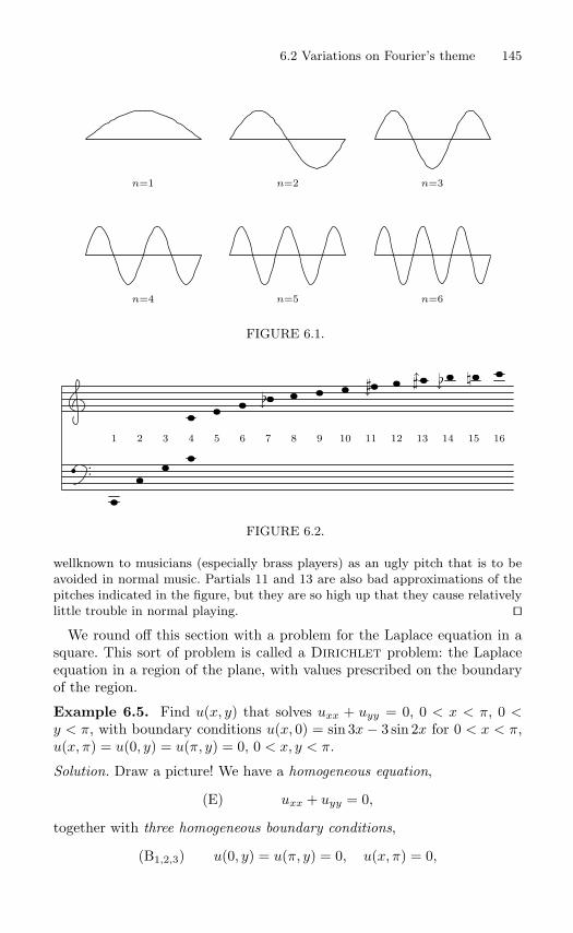
6.2 Variations on Fourier’s theme 145
n=1 n=2 n=3
n=4 n=5 n=6
FIGURE 6.1.
• ..
•••• •• ••
•• •• •• •• •• •• •• •• •• •• •• •• ••↓
↓ ↑↓
1 2 3 4 5 6 7 8 9 10 11 12 13 14 15 16
FIGURE 6.2.
wellknown to musicians (especially brass players) as an ugly pitch that is to beavoided in normal music. Partials 11 and 13 are also bad approximations of thepitches indicated in the figure, but they are so high up that they cause relativelylittle trouble in normal playing.
We round off this section with a problem for the Laplace equation in asquare. This sort of problem is called a Dirichlet problem: the Laplaceequation in a region of the plane, with values prescribed on the boundaryof the region.
Example 6.5. Find u(x, y) that solves uxx + uyy = 0, 0 < x < π, 0 <y < π, with boundary conditions u(x, 0) = sin 3x− 3 sin 2x for 0 < x < π,u(x, π) = u(0, y) = u(π, y) = 0, 0 < x, y < π.
Solution. Draw a picture! We have a homogeneous equation,
(E) uxx + uyy = 0,
together with three homogeneous boundary conditions,
(B1,2,3) u(0, y) = u(π, y) = 0, u(x, π) = 0,
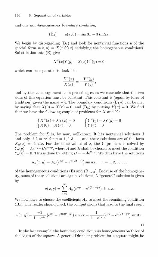
146 6. Separation of variables
and one non-homogeneous boundary condition,
(B4) u(x, 0) = sin 3x− 3 sin 2x.
We begin by disregarding (B4) and look for nontrivial functions u of thespecial form u(x, y) = X(x)Y (y) satisfying the homogeneous conditions.Substitution into (E) gives
X ′′(x)Y (y) +X(x)Y ′′(y) = 0,
which can be separated to look like
X ′′(x)X(x)
= −Y ′′(y)Y (y)
,
and by the same argument as in preceding cases we conclude that the twosides of this equation must be constant. This constant is (again by force oftradition) given the name −λ. The boundary conditions (B1,2) can be metby saying that X(0) = X(π) = 0, and (B3) by putting Y (π) = 0. We findthat we have the following couple of problems for X and Y :
X ′′(x) + λX(x) = 0X(0) = X(π) = 0
Y ′′(y) − λY (y) = 0Y (π) = 0
The problem for X is, by now, wellknown. It has nontrivial solutions ifand only if λ = n2 for n = 1, 2, 3, . . ., and these solutions are of the formXn(x) = sinnx. For the same values of λ, the Y problem is solved byYn(y) = Aeny+Be−ny, whereA andB shall be chosen to meet the conditionYn(π) = 0. This is done by letting B = −Ae2nπ. We thus have the solutions
un(x, y) = An
(eny − en(2π−y)) sinnx, n = 1, 2, 3, . . . ,
of the homogeneous conditions (E) and (B1,2,3). Because of the homogene-ity, sums of these solutions are again solutions. A “general” solution is givenby
u(x, y) =∞∑
n=1
An
(eny − en(2π−y)) sinnx.
We now have to choose the coefficients An to meet the remaining condition(B4). The reader should check the computations that lead to the final result
u(x, y) =−3
1 − e4π
(e2y − e2(2π−y)) sin 2x+
11 − e6π
(e3y − e3(2π−y)) sin 3x.
In the last example, the boundary condition was homogeneous on three of
the edges of the square. A general Dirichlet problem for a square might be

6.2 Variations on Fourier’s theme 147
taken care of by solving four problems of this kind, with non-homogeneousboundary values on one edge at a time, and adding the solutions.
In the exercises the reader will have the opportunity to apply the basicideas of the method of separation of variables to a variety of problems. Inall cases, the success of the method is coupled to the fact that one reachesa problem for an ordinary differential equation together with boundaryconditions. This problem turns out to have nontrivial solutions only forcertain values of the “separation constant,” and these solutions are a sort ofbuilding blocks out of which the solutions are constructed. This sort of ODEproblem is called a Sturm–Liouville problem and will be considered inSec. 6.4 for its own sake.
It is even possible to treat partial differential equations with more thantwo independent variables in much the same way.
Exercises6.3 Find a solution of the heat problem ut = uxx for 0 < x < π, t > 0, such
that ux(0, t) = ux(π, t) = 0 for t > 0 and u(x, 0) = 12 (1 + cos 3x) for
0 < x < π.
6.4 Determine a solution of the problemuxx = t ut, 0 < x < π, t > 1;u(0, t) = u(π, t) = 0, t > 1,u(x, 1) = sinx+ 2 sin 3x, 0 < x < π.
6.5 Find a solution of the non-homogeneous heat conduction problemuxx = ut + sinx, 0 < x < π, t > 0;u(0, t) = u(π, t) = 0, t > 0;u(x, 0) = sinx+ sin 2x, 0 < x < π.
6.6 Solve the following problem for the vibrating string:uxx = utt, 0 < x < π, t > 0;u(x, 0) = 3 sin 2x, ut(x, 0) = 5 sin 3x, 0 < x < π;u(0, t) = u(π, t) = 0, t > 0.
6.7 The plucked string: a point on the string is pulled from its resting positionand then released with no initial speed. If the string is plucked at its middlepoint, what tones are heard? In a mathematical formulation: Solve theproblem (6.11), when f is given by
f(x) = ax, 0 ≤ x ≤ 12 π, f(x) = a(π − x), 1
2 π ≤ x ≤ π,
and g(x) = 0.
6.8 Find u(x, t) ifuxx(x, t) = utt(x, t), 0 < x < 1, t > 0;u(0, t) = u(1, t) = 0, t > 0;u(x, 0) = sin 3πx, ut(x, 0) = sinπx cos2 πx, 0 < x < 1.

148 6. Separation of variables
6.9 Find a solution of the following problem (one-dimensional heat conductionwith loss of heat to the surrounding medium) for h > 0 constant: ut =uxx − hu, 0 < x < π, t > 0, together with u(0, t) = 0, u(π, t) = 1 for t > 0and u(x, 0) = 0 for 0 < x < π.
6.10 A Dirichlet problem: uxx + uyy = 0 for 0 < x, y < 1, u(x, 0) = u(x, 1) = 0,u(0, y) = 0 and u(1, y) = sin3 πy.
6.11 Find a solution u = u(x, t) of this problem:uxx + 1
4 u = ut, 0 < x < π, t > 0;u(0, t) = 0, u(π, t) = 1, t > 0;u(x, 0) = 0, 0 < x < π.
6.3 The Dirichlet problem in the unit disk
We shall study a problem for the Laplace equation in two dimensions. Letu = u(x, y) be a function defined in an open, connected set Ω in R2. TheLaplace equation in Ω is
∆u :=∂2u
∂x2 +∂2u
∂y2 = 0, (x, y) ∈ Ω.
The solutions of this equation are called harmonic functions in Ω. TheDirichlet problem is the task of finding all such functions with prescribedvalues on the boundary ∂Ω. We shall study this problem in the case whenΩ is the unit disk D : x2 + y2 < 1, so that the boundary ∂Ω is the unitcircle T : x2 + y2 = 1. Concisely, the problem is
∆u(x, y) = 0, (x, y) ∈ D; u(x, y) = g(x, y) = known function, (x, y) ∈ T.(6.13)
We shall describe two lines of attack: first a method that requires know-ledge of the elementary theory of analytic (or holomorphic) functions, thena different approach involving separation of variables.
Method 1. Interpret (x, y) as a complex number z = reiθ. The boundaryfunction g can then conveniently be considered as a function of the polarcoordinate θ, so that we are looking for harmonic functions u = u(z) =u(reiθ) for r < 1 with boundary values
u(eiθ) = limr1
u(reiθ) = g(θ), −π < θ ≤ π.
The unit disk D is simply connected. By the theory of analytic functions,every harmonic function u in D has a conjugate-harmonic partner v suchthat the expression f(z) = u(z) + iv(z) is analytic in D. An analytic func-tion in the unit disk is the sum of a power series:
u(z) + iv(z) = f(z) =∞∑
n=0
Anzn =
∞∑n=0
Anrn einθ
6.3 The Dirichlet problem in the unit disk 149
=∞∑
n=0
(Bn + iCn) rn (cosnθ + i sinnθ)
=∞∑
n=0
rn((Bn cosnθ − Cn sinnθ) + i(Cn cosnθ +Bn sinnθ)
),
where the An are Taylor coefficients with real parts Bn and imaginary partsCn. Taking the real part of the whole equation one sees that u(z) must berepresentable by a series of the form
u(z) = u(reiθ) =∞∑
n=0
rn(Bn cosnθ − Cn sinnθ
),
and, conversely, one realizes (by reading the equation backward) that allsuch series represent harmonic functions (provided the corresponding series∑Anz
n converges in D).In order to make the formula neater, we switch letters: put an = Bn and
bn = −Cn for n ≥ 1, a0 = 2B0, and note that the value of C0 is immaterial(since sin 0θ = 0 for all θ), and we get
u(reiθ) = 12 a0 +
∞∑n=1
rn(an cosnθ + bn sinnθ
).
Method 2. We want to find solutions of the Laplace equation in the regiondescribed in polar coordinates by r < 1, −π ≤ θ ≤ π. First we transformthe equation into polar coordinates. Using the chain rule one finds that∆u = 0 (for r > 0) is equivalent to
r∂
∂r
(r∂u
∂r
)+∂2u
∂θ2= 0
(the computations required are usually carried through in calculus text-books as examples of the chain rule). We then proceed to find nontrivialsolutions of the special form u(r, θ) = R(r) Θ(θ), i.e., solutions that areproducts of one function of r and one function of θ. Substitution into theequation results in
r∂
∂r
(rdR
drΘ(θ)
)+R(r)
d2Θdθ2
= 0 ⇐⇒ r(rR′)′Θ = −RΘ′′.
We divide by RΘ and get
1Rr(rR′)′ = −Θ′′
Θ.
The left-hand member in this equation is independent of θ and the right-hand member is independent of r. Just as in Sec. 1.4 we can conclude that

150 6. Separation of variables
both members must then be constant, and this constant value is called λ.The situation splits into the two ordinary differential equations
Θ′′ + λΘ = 0, r(rR′)′ − λR = 0.
In addition, there are a couple of “boundary conditions”: in order that thefunction u = RΘ be uniquely determined in D, the function Θ(θ) musthave period 2π. Furthermore, since u shall have a finite value at the origin,we demand that R(r) have a finite limit R(0+) as r 0 .
We begin with the problem for Θ:Θ′′(θ) + λΘ(θ) = 0,Θ(θ + 2π) = Θ(θ) for all θ.
As in Sec. 1.4, we work through the cases λ < 0, λ = 0 and λ > 0. Inthe first case there are no periodic solutions (except for Θ(θ) ≡ 0). Inthe case λ = 0, all constant functions will do: Θ0(θ) = A0. When λ > 0,let λ = ω2 with ω > 0, and we find the solutions Θω(θ) = Aω cosωθ +Bω sinωθ. These have period 2π precisely if ω is a positive integer: ω = n,n = 1, 2, 3, . . .. Summarizing, we have found interesting solutions of the Θproblem precisely when λ = n2, n = 0, 1, 2, . . ..
For these λ we solve the R-problem. When λ = 0, the equation becomes
r(rR′)′ = 0 ⇐⇒ rR′ = C ⇐⇒ R′ =
C
r⇐⇒ R = C ln r +D.
The value R(0+) exists only if C = 0. In this case we thus have a solutionu = u0 = Θ0(θ)R0(r) = A0 ·D = constant. For reasons that will presentlybecome evident we denote this constant by 1
2a0.When λ = n2 with n > 0 we have a so-called Euler equation:
r(rR′)′ = n2R ⇐⇒ r2R′′ + rR′ − n2R = 0.
To solve it, we change the independent variable by putting r = es, whichresults in
d2R
ds2− n2R = 0,
which has the solutions R = Cens +De−ns = Crn +Dr−n. We must takeD = 0 to ascertain that R(0+) exists. Piecing together with Θ we arriveat the solution
u(reiθ) = un(reiθ) = Θn(θ)Rn(r) =Cn rn (An cosnθ +Bn sinnθ)
= rn (an cosnθ + bn sinnθ).
The Laplace equation is homogeneous. Assuming convergence for theseries, the solutions of ∆u = 0 in the unit disk should be representable byseries of the form
u(reiθ) = 12 a0 +
∞∑n=1
rn(an cosnθ + bn sinnθ
).

6.3 The Dirichlet problem in the unit disk 151
This is the same form for harmonic functions in D as obtained by “Method1” above.
The formal solutions that we have obtained can, of course, also be writtenin “complex” form. Via Euler’s formulae we find
u(r, θ) = u(reiθ) =∑n∈Z
cnr|n|einθ. (6.14)
Notice that the exponents on r have a modulus sign.Now we turn to the boundary condition. As r 1, we wish that the
values of the solution approach a prescribed function g(θ). For simplicity, weassume that g is continuous. Let the numbers cn be the Fourier coefficientsof g:
cn =12π
∫Tg(θ) e−inθ dθ,
and, using these coefficients, form the function u(r, θ) as in (6.14). ByLemma 4.1, there exists a number M such that |cn| ≤ M . Using the Weier-strass M -test we can easily conclude that the series defining u convergesabsolutely and uniformly in every inner closed circular disk r ≤ r0, wherer0 < 1, and this still holds after differentiations with respect to r as well asθ. According to the theorem on differentiation of series, termwise differenti-ation is thus possible, and since each term of the series satisfies the Laplaceequation and this equation is homogeneous, the sum function u will alsosatisfy the same equation. Now we turn to the boundary condition. Theuniform convergence in r ≤ r0 allows us to interchange the order of sumand integral in the following formula:
u(r, θ) =∑n∈Z
cn r|n| einθ =
∑n∈Z
r|n| einθ 12π
∫Tg(t) e−int dt
=∫T
(12π
∑n∈Z
r|n| ein(θ−t)
)g(t) dt.
The sum in brackets can be computed explicitly – it is made up of twogeometric series:
∑n∈Z
r|n| eins =−1∑
n=−∞r−n eins +
∞∑n=0
rn eins
=∞∑
n=1
rn e−ins +∞∑
n=0
rn eins =r e−is
1 − r e−is+
11 − r eis
=(1 − reis)re−is + 1 − re−is
|1 − r eis|2 =1 − r2
1 + r2 − 2r cos s.

152 6. Separation of variables
We define the Poisson kernel to be the function
Pr(s) = P (s, r) =12π
∑n∈Z
r|n| eins =12π
· 1 − r2
1 + r2 − 2r cos s.
This gives the following formula for u:
u(r, θ) =∫TPr(θ − t) g(t) dt =
∫TPr(t) g(θ − t) dt.
The Poisson kernel has some interesting properties:
1. Pr(s) = Pr(−s) ≥ 0 for r < 1, s ∈ T.
2.∫T Pr(s) ds = 1 for r < 1.
3. If δ > 0, then
limr1
∫ π
δ
Pr(s) ds = 0.
The proofs of 1 and 2 are simple (2 follows by integrating the series termby term, which is legitimate). The property 3 can be shown thus: sincePr(s) is decreasing as s goes from 0 to π, we have Pr(s) ≤ Pr(δ) on theinterval, and∫ π
δ
Pr(s) ds ≤ Pr(δ)∫ π
δ
ds = (π − δ)Pr(δ) → 0 as r 1.
This sort of properties of a collection of functions should be familiar to thereader. They actually amount to the fact that Pr is a positive summationkernel of the kind studied in Sec. 2.4. The only difference is the fact thatthe present kernel is “numbered” by a variable r that tends to 1, insteadof using an integer N tending to infinity. Theorem 2.1 can be used, and weget the result that we have constructed a solution of the Dirichlet problemwith boundary values g(θ) in the sense that
limr1
u(r, θ) = g(θ)
at all points θ where g is continuous.In addition, the solution is actually unique. This can be proved using
a technique similar to that employed at the end of Sec. 4.2. First oneproves that the problem with boundary values identically zero has only thesolution identically zero, and then this is applied to the difference of twosolutions corresponding to the same boundary values.
Remark. We have here touched upon another method of summing series thatmay not be convergent. It is called Poisson or Abel summation. For a numericalseries
∑∞n=0 an it consists in forming the function
f(r) =∞∑
n=0
anrn, 0 < r < 1.

6.4 Sturm–Liouville problems 153
If this function exists in the interval indicated, and if it has a limit as r 1, thenthis limit is called the Poisson or Abel sum of the series. It can be proved that thismethod sums a convergent series to its ordinary sum. It is also a quite powerfulmethod: it is stronger than Cesaro summation in the sense that every Cesarosummable series is also Abel summable; and there exist series summable by Abelthat are not summable by Cesaro, not even after any number of iterations.
Example 6.6. Find a solution of the Dirichlet problem in the disk havingboundary values u(1, θ) = cos 4θ − 1. Express the solution in rectangularcoordinates!
Solution. It is immediately seen that in polar coordinates the solution mustbe
u(r, θ) = −1 + r4 cos 4θ.
We rewrite the cosine to introduce cos and sin of the single value θ:
u= −1 + r4(cos2 2θ − sin2 2θ)= −1 + r4((cos2 θ − sin2 θ)2 − (2 sin θ cos θ)2)= −1 + r4(cos4 θ − 2 cos2 θ sin2 θ + sin4 θ − 4 sin2 θ cos2 θ)= −1 + x4 − 6x2y2 + y4.
Exercises
6.12 Find a solution of the Dirichlet problem in the unit disk such that u(eiθ) =2 + cos 3θ + sin 4θ.
6.13 Find a solution of the same problem such that u(x, y) = x4 + y4 forx2 + y2 = 1.
6.14 Solve the Dirichlet problem with boundary values u(1, θ) = sin3 θ.
6.15 Perform the details of the proof of the uniqueness of the solution of Dirich-let’s problem.
6.4 Sturm–Liouville problems
In our solutions of the problems in the preceding sections, a central role wasplayed by a boundary value problem for an ordinary differential equationcontaining a parameter λ. This problem proved to have nontrivial solu-tions for certain values of λ, but these values had the character of being“exceptional”. The situation seems loosely similar to a kind of problem thatthe reader should have been faced with in a seemingly completely differentcontext, namely linear algebra: eigenvalue problems for an operator or amatrix. We shall see that this similarity is really not loose at all!

154 6. Separation of variables
We start with a few definitions. Let V be a space with an inner product〈·, ·〉. A linear mapping A, defined in some subspace DA of V and having itsvalues in V , is called an operator on V . Notice that this definition is slightlydifferent from the one that is common in the case of finite-dimensionalspaces: we do not demand that the domain of definition of the operator bethe entire space V . We write V ⊇ DA
A−→ V or A : DA → V . The imageof a vector u ∈ DA is written A(u) or, mostly, simply Au.
Definition 6.1 An operator A : DA → V is said to be symmetric, if
〈Au, v〉 = 〈u,Av〉 for all u, v ∈ DA.
Example 6.7. Let V = L2(T), DA = V ∩C2(T) and let A be the operator−D2, so that Au = −u′′. Since u ∈ C2(T), the image Au is a continuousfunction and thus belongs to V . We have
〈Au, v〉 = −∫Tu′′(x) v(x) dx = −[u′(x) v(x)
]π−π
+∫Tu′(x) v′(x) dx
=[u(x) v′(x)
]π−π
−∫Tu(x) v′′(x) dx = 〈u,Av〉.
The integrated parts are zero, because all the functions are periodic andthus have the same values at −π and π. Definition 6.2 An operator A : DA → V is said to have an eigenvalue λ,if there exists a vector u ∈ DA such that u = 0 and Au = λu. Such a vectoru is called an eigenvector, more precisely, an eigenvector belonging to theeigenvalue λ. The set of eigenvectors belonging to a particular eigenvalueλ (together with the zero vector) make up the eigenspace belonging to λ.
Example 6.8. We return to the situation in Example 6.7. If u(x) =a cosnx+b sinnx, where a and b are arbitrary constants and n is an integer≥ 0, then clearly Au = n2u. In this situation we have thus the eigenvaluesλ = 0, 1, 4, 9, . . .. For λ = 0, the eigenspace has dimension 1 (it consists ofthe constant functions), for the other eigenvalues the dimension is 2. (Thefact that this is the complete story of the eigenvalues of this operator wasshown in Sec. 6.3, “Method 2.”)
For symmetric operators on a finite-dimensional space there is a spectraltheorem, which is a simple adjustment to the case of complex scalars of thetheorem from real linear algebra: If A is a symmetric operator defined on allof Cn (for example), then there is an orthogonal basis for Cn, consistingof eigenvectors for A. The proof of this can be performed as a replica ofthe corresponding proof for the real case (if anything, the complex case israther easier to do than a purely “real” proof). In infinite dimensions thingsare more complicated, but in many cases similar results do hold there aswell.
First we give a couple of simple results that do not depend on dimension.
6.4 Sturm–Liouville problems 155
Lemma 6.1 A symmetric operator has only real eigenvalues, and eigen-vectors corresponding to different eigenvalues are orthogonal.
Proof. Suppose that Au = λu and Av = µv, where u = 0 and v = 0. Thenwe can write
λ〈u, v〉 = 〈λu, v〉 = 〈Au, v〉 = 〈u,Av〉 = 〈u, µv〉 = µ〈u, v〉. (6.15)
First, choose v = u, so that also µ = λ, and we have that λ‖u‖2 = λ‖u‖2.Because of u = 0 we conclude that λ = λ, and thus λ is real. It followsthat all eigenvalues must be real. But then we can return to (6.15) with theinformation that µ is also real, and thus (λ−µ)〈u, v〉 = 0. If now λ−µ = 0,then we must have that 〈u, v〉 = 0, which proves the second assertion.
Regrettably, it is not easy to prove in general that there are “sufficientlymany” eigenvectors (to make it possible to construct a “basis,” as in finitedimensions). We shall here mention something about one situation wherethis does hold, the study of which was initiated by Sturm and Liouville
during the nineteenth century. As special cases of this situation we shallrecognize some of the boundary value problems studied in this text, startingin Sec. 1.4.
We settle on a compact interval I = [a, b]. Let p ∈ C1(I) be a real-valuedfunction such that p(a) = 0 = p(b); let q ∈ C(I) be another real-valuedfunction; and let w ∈ C(I) be a positive function on the same interval(i.e., w(x) > 0 for x ∈ I). We are going to study the ordinary differentialequation
(E) (pu′)′ + qu+ λwu = 0 ⇐⇒d
dx
(p(x)
du
dx
)+ q(x)u(x) + λw(x)u(x) = 0, x ∈ I.
Here, λ is a parameter and u the “unknown” function. Furthermore, weshall consider boundary conditions, initially of the form
(B) A0u(a) +A1u′(a) = 0, B0u(b) +B1u
′(b) = 0.
Here, Aj and Bj are real constants such that (A0, A1) = (0, 0) = (B0, B1).
Remark. If we take p(x) = w(x) = 1, q(x) = 0, A0 = B0 = 1 and A1 = B1 = 0,we recover the problem studied in Sec. 1.4.
The problem (E)+(B) is called a regular Sturm–Liouville problem. Weintroduce the space L2(I, w), where w is the function occurring in (E). Thismeans that we have an inner product
〈u, v〉 =∫
I
u(x) v(x)w(x) dx.
In particular, all functions u ∈ C(I) will belong to L2(I, w), since theinterval is compact.

156 6. Separation of variables
We define an operator A by the formula
Au = − 1w
((pu′)′ + qu
),
DA = u ∈ C2(I) : Au ∈ L2(I, w) and u satisfies (B).Then, (E) can be written simply as Au = λu. The problem of finding non-trivial solutions of the problem (E)+(B) has been rephrased as the problemof finding eigenvectors of the operator A. (The fact that DA is a linear spaceis a consequence of the homogeneity of the boundary conditions.)
The symmetry of A can be shown as a slightly more complicated parallelof Example 6.7 above. On the one hand,
〈Au, v〉 = −b∫
a
1w
((pu′)′ + qu
)v w dx = −
b∫a
((pu′)′ + qu)v dx
= −b∫
a
(pu′)′v dx−b∫
a
q u v dx = −[p u′ v]ba
+
b∫a
(p u′v′ − q u v) dx.
On the other hand (using the fact that p, q and w are real-valued),
〈u,Av〉 =
b∫a
u ·(
− 1w
)((pv′)′ + qv
)w dx = −
b∫a
u(p v′)′ dx−b∫
a
u q v dx
= −[u p v′]ba
+
b∫a
(u′ p v′ − u q v) dx.
We see that
〈Au, v〉 − 〈u,Av〉 =[puv′ − pu′v
]ba
=
[p(x)
∣∣∣∣∣u(x) u′(x)
v(x) v′(x)
∣∣∣∣∣]x=b
x=a
.
But the determinant in this expression, for x = a, must be zero: indeed, weassume that both u and v satisfy the boundary condition (B) at a, whichmeans that
A0u(a) +A1u′(a) = 0,
A0v(a) +A1v′(a) = 0.
This can be considered to be a homogeneous linear system of equationswith (the real numbers) A0 and A1 as unknowns, and it has a nontrivialsolution (since we assume that (A0, A1) = (0, 0)). Thus the determinant iszero. In the same way it follows that the determinant is zero at x = b. Weconclude then that
〈Au, v〉 = 〈u,Av〉,

6.4 Sturm–Liouville problems 157
so that A is symmetric.In this case, the symmetry is achieved by the fact that a certain substi-
tution of values results in zero at each end of the interval. Clearly, this isnot necessary. An operator can be symmetric for other reasons, too. Weshall not delve deeper into this in this text, but refer the reader to textson ordinary differential equations.
For the case we have sketched above, the following result holds.
Theorem 6.1 (Sturm–Liouville’s theorem) The operator A, belong-ing to the problem (E)+(B), has infinitely many eigenvalues, which canbe arranged in an increasing sequence:
λ1 < λ2 < λ3 < · · · , where λn → ∞ as n → ∞.
The eigenspace of each eigenvalue has dimension 1, and if ϕn is an eigen-vector corresponding to λn, then ϕn∞
n=1 is a complete orthogonal systemin L2(I, w).
This can be rewritten to refer directly to the differential equation prob-lem:
Theorem 6.2 The problem (E)+(B) has solutions for an infinite num-ber of values of the parameter λ, which can be arranged in an increasingsequence:
λ1 < λ2 < λ3 < · · · , where λn → ∞ as n → ∞.
For each of these values of λ, the solutions make up a one-dimensionalspace, and if ϕn is a non-zero solution corresponding to λn, the set ϕn∞
n=1is a complete orthogonal system in L2(I, w).
Proofs can be found in texts on ordinary differential equations.It is of considerable interest that one gets a complete orthogonal system.
We already know this to be true in a couple of special cases. First we havethe problem
u′′(x) + λu(x) = 0, 0 < x < π; u(0) = u(π) = 0, (6.16)
that we first met already in Sec. 1.4; here the eigenfunctions are ϕn(x) =sinnx, and according to Sec. 5.4 these are complete in L2(0, π) (with weightfunction 1). Secondly, we have seen this problem, treated in Example 6.1of Sec. 6.2:
u′′(x) + λu(x) = 0, 0 < x < π; u′(0) = u′(π) = 0. (6.17)
There we found the eigenfunctions ϕ0(x) = 12 and ϕn(x) = cosnx, and we
have seen that they are also complete in L2(0, π).

158 6. Separation of variables
In the exercises, the reader is invited to investigate a few more problemsthat fall within the conditions of Theorem 6.2.
If the assumptions are changed, the results may deviate from those ofTheorem 6.2. We have already seen this in Examples 6.7 and 6.8 of thepresent section. There, we studied the operator −D2 on T, which corre-sponds to the problem
u′′(x) + λu(x) = 0, −π ≤ x ≤ π; u(−π) = u(π), u′(−π) = u′(π).
The boundary conditions are of a different character from (B): they meanthat u and u′ have periodic extensions with period 2π (so that they cantruly be considered to be functions on the unit circle T). They are alsocommonly called periodic boundary conditions. (In contrast, the conditionsconsidered in (B) are said to be separated: the values at a and b have noconnection with each other.) In this case the eigenspaces (except for one)have dimension 2. If we choose orthogonal bases in each of the eigenspacesand pool all these together, the result is again a complete system in therelevant space, which is L2(T).
Yet another few examples are given in the next section. In one of thesecases it happens that the function p goes to zero at the ends of the compactinterval; in others the interval is no longer compact. It can be finite, butopen, and one or more of the functions p, q, and w may have singularities atthe ends; the interval may also be a half-axis or even the entire real line. Allthese situations give rise to what are known as singular Sturm–Liouvilleproblems, and they sometimes occur when treating classical situations forpartial differential equations.
Exercises
6.16 Determine a complete orthogonal system in L2(0, π) consisting of solutionsof the problem
u′′(x) + λu(x) = 0, 0 < x < π; u(0) = u′(π) = 0.
6.17 The same problem, but with boundary conditions
u(0) = u(π) + u′(π) = 0.
6.18 Show that the problem
d
dx
(√1 − x2 du
dx
)+
λ√1 − x2
u(x) = 0, −1 < x < 1
has the eigenvalues λ = n2 (n = 0, 1, 2, . . .) and eigenfunctions Tn(x) =cos(n arccosx) for λ = n2. (You are not expected to prove that these areall the eigenvalues and eigenfunctions of the problem.)
6.5 Some singular Sturm–Liouville problems 159
6.5 Some singular Sturm–Liouville problems
Some celebrated problems in classical physics lead up to problems for or-dinary differential equations that are similar to the problems consideredin the preceding section. We review some of these problems here, partlybecause of their historical interest, but also because they have solutionsthat are polynomials that we met in Sec. 5.5–6.
The Legendre polynomials are solutions of the following singular Sturm–Liouville problem. Let I = [−1, 1] and study the problem
d
dx
((1 − x2)u′(x)
)+ λu(x) = 0, −1 < x < 1,
with no boundary conditions at all (except that u(x) should be definedin the closed interval). Here we can identify p(x) = 1 − x2, q(x) = 0 andw(x) = 1. Since p(x) = 0 at both ends of the interval, the correspondingoperator A will be symmetric if one takes DA = u ∈ C2(I) : Au ∈ L2(I)(the reader should check this, which is not difficult). It can be proved thatthis problem has eigenvalues λ = n(n + 1), n = 0, 1, 2, . . ., and that theeigenfunctions are actually (multiples of) the Legendre polynomials.
Remark. The origin of this problem is the three-dimensional Laplace equationin spherical coordinates (r, θ, φ), defined implicitly by
x = r sinφ cos θy = r sinφ sin θz = r cosφ
r ≥ 0,0 ≤ φ ≤ π,
−π < θ ≤ π.
In these coordinates, the equation takes the form
∆u ≡ ∂2u
∂r2+
2r
∂u
∂r+
1r2
∂2u
∂φ2 +cotφr2
∂u
∂φ+
1r2 sin2 φ
∂2u
∂θ2= 0.
This can also be written as
r(ru)
rr+
1sinφ
(sinφ uφ
)φ
+1
sin2 φuθθ = 0. (6.18)
A function f(x, y, z) is said to be homogeneous of degree n, if f(tx, ty, tz) =tnf(x, y, z) for t > 0. This means that f is completely determined by its valueson, say, the unit sphere, so that it can be written f(x, y, z) = rng(φ, θ) for acertain function g. We now look for solutions un of (6.18) that are homogeneousof degree n; these solutions are called spherical harmonics. Write
un(x, y, z) = rnSn(φ, θ),
where Sn is called a spherical surface harmonic. Substitution into (6.18) andsubsequent division by rn gives
(n+ 1)nSn +1
sinφ∂
∂φ
(sinφ
∂Sn
∂φ
)+
1sin2 φ
∂2Sn
∂θ2= 0.

160 6. Separation of variables
Now we specialize once more and restrict ourselves to solutions Sn that are in-dependent of θ; denote them by Zn(φ). The equation reduces to
(n+ 1)nZn +1
sinφd
dφ
(sinφ
dZn
dφ
)= 0. (6.19)
Finally, we put x = cosφ and Pn(x) = Zn(φ). The reader is asked (in Exer-cise 6.19) to check that the equation ends up as
(1 − x2)P ′′(x) − 2xP ′(x) + n(n+ 1)Pn(x) = 0. (6.20)
This is the Legendre equation. The Laguerre polynomials are solutions of the following singular Sturm–
Liouville problem. Take I = [0,∞[, p(x) = x e−x, q(x) = 0 and w(x) = e−x.The differential equation is
d
dx
(x e−x u′(x)
)+ λ e−x u(x) = 0 ⇐⇒
xu′′(x) + (1 − x)u′(x) + λu(x) = 0, x ≥ 0,
and the “boundary conditions” are that u(0) shall exist (of course) andthat u(x)/xm shall tend to 0 as x → ∞ for some number m. (The lattercondition can be phrased thus: u(x) is majorized by some power of x, asx → ∞, or u(x) “increases at most like a polynomial”.) The eigenvalues ofthis problem are λ = n = 0, 1, 2, . . ., and the Laguerre polynomials Ln areeigenfunctions.
The Hermite polynomials come from the following singular Sturm–Liou-ville problem. On I = R one studies the equation
d
dx
(e−x2
u′(x))
+ λ e−x2u(x) = 0
with the “boundary condition” that the solutions are to satisfy u(x)/xm →0 as |x| → ∞ for some m > 0. Eigenvalues are the numbers λ = 2n,n = 0, 1, 2, . . . and the Hermite polynomials Hn are eigenfunctions.
Exercise
6.19 Check that the change of variable x = cosφ does transform the equation(6.19) into (6.20).
Summary of Chapter 6
The Method of Separation of VariablesGiven a linear partial differential equation of order 2, with independent vari-ables (x, y) and unknown function u(x, y), together with boundary and/orinitial conditions—

Historical notes 161
1. If necessary (and possible), homogenize the equation and as many aspossible of the other conditions.
2. Look for solutions of the homogeneous sub-problem having the par-ticular form u(x, y) = X(x)Y (y). This normally leads to a Sturm–Liouville problem, and the result should be a sequence of solutionsun = un(x, y) = Xn(x)Yn(y), n = 1, 2, 3, . . ..
3. The homogeneous problem has the “general” solution u =∑cnun,
where the cn are constants.
4. Adapt the constants cn to make the solutions satisfy also the non-homogeneous conditions.
5. If you began by homogenizing the problem, don’t forget to re-adaptthe solution to suit the original problem.
DefinitionAssume p, q real, w > 0 on an interval I = [a, b]. Then the following is aregular Sturm–Liouville problem on I:
(pu′)′ + qu+ λwu = 0A0u(a) +A1u
′(a) = 0, B0u(b) +B1u′(b) = 0
With the Sturm–Liouville problem we associate the operator A, defined forfunctions u that satisfy the boundary conditions by the formula
Au = − 1w
((pu′)′ + qu
).
Theorem(The Sturm–Liouville theorem) The operator A, belonging to the Sturm–Liouville problem, has infinitely many eigenvalues, which can be arrangedin an increasing sequence:
λ1 < λ2 < λ3 < · · · , where λn → ∞ as n → ∞.
The eigenspace of each eigenvalue has dimension 1, and if ϕn is an eigen-vector corresponding to λn, then ϕn∞
n=1 is a complete orthogonal systemin L2(I, w).
Formulae for orthogonal polynomials are found on page 254 f.
Historical notes
Jacques Charles Francois Sturm (1803–55) and Joseph Liouville (1809–82) both worked in Paris. Sturm was chiefly concerned with differential equations;Liouville also did remarkable work in the field of analytic functions and the theoryof numbers.

162 6. Separation of variables
Problems for Chapter 6
6.20 Using separation of variables, solve the problem ut = uxx, 0 < x < 1, t > 0;u(0, t) = 1, u(1, t) = 3, u(x, 0) = 2x+ 1 − sin 2πx.
6.21 Find a solution of the problem
uxx = utt + 2ut, 0 < x < π, t > 0;
u(0, t) = u(π, t) = 0, t > 0;
u(x, 0) = 0, ut(x, 0) = sin3 x, 0 < x < π.
6.22 Find a solution of the differential equation uxx = ut + u, 0 < x < π, t > 0,that satisfies the boundary conditions u(0, t) = u(π, t) = 0, t > 0, andu(x, 0) = x(π − x), 0 < x < π.
6.23 Find a function u(x, t) such thatut = 4uxx, 0 < x < 4, t > 0;
u(0, t) = 10, u(4, t) = 50, t > 0;
u(x, 0) = 30, 0 < x < 4.
6.24 Find a solution of the following problem:uxx = utt, 0 < x < π, t > 0;
u(0, t) = u(π, t) = 0, t > 0;
u(x, 0) = x(π − x), 0 < x < π;
ut(x, 0) = sin 2x, 0 < x < π.
6.25 Determine a solution of the boundary value problemuxx + uyy = x, 0 < x < 1, 0 < y < 1;
u(x, 0) = u(x, 1) = 0, 0 < x < 1;
u(0, y) = u(1, y) = 0, 0 < y < 1.
6.26 Find a solution in the form of a series to the Dirichlet problemuxx + uyy = 0, x2 + y2 < 1;
u(x, y) = |x|, x2 + y2 = 1.
6.27 Solve the following problem for the two-dimensional Laplace equationuxx + uyy = 0, 0 < x < π, 0 < y < π;
ux(0, y) = ux(π, y) = 0, 0 < y < π;
u(x, 0) = sin2 x, u(x, π) = 0, 0 < x < π.
6.28 Find a function u(x, t) such that
ut = uxx + cosx, 0 < x < π, t > 0;
ux(0, t) = ux(π, t) = 0, t > 0; u(x, 0) = cos2 x+ 2 cos4 x, 0 < x < π.

Problems for Chapter 6 163
6.29 Solve the following problem for a modified wave equation:
uxx = utt + 2ut, 0 < x < π, t > 0;
u(0, t) = u(π, t) = 0, t > 0,
u(x, 0) = sinx+ sin 3x, ut(x, 0) = 0, 0 < x < π.
6.30 Find u = u(x, t) that satisfies the equation uxx = ut + tu, 0 < x < π,t > 0, with boundary conditions u(0, t) = u(π, t) = 0 for t > 0 and initialcondition u(x, 0) = sin 2x, 0 < x < π.
6.31 Find a bounded solution of the problem for a vibrating beam:utt + uxxxx = 0, 0 < x < π, t > 0;
u(0, t) = u(π, t) = uxx(0, t) = uxx(π, t) = 0, t > 0;
u(x, 0) = x(π − x), ut(x, 0) = 0, 0 < x < π.
6.32 A (very much) simplified model of a nuclear reactor is given by the problemut = Auxx +Bu, 0 < x < l, t > 0;
u(0, t) = u(l, t) = 0, t > 0.
Here, u is the concentration of neutrons, while A and B are positive con-stants. The term Auxx describes the scattering of neutrons by diffusion,and the term Bu the creation of neutrons through fission. Prove that thereis a critical value L of the length l such that if l > L, then there existunbounded solutions; whereas if l < L, then all solutions are bounded.
6.33 In order to get good tone quality from a piano, it is desirable to havevibrations rich in overtones. An exception is the seventh partial, whichresults in musical dissonance, and should thus be kept low. Under certainidealizations the vibrations of a piano string are described by
utt = uxx, 0 < x < π, t > 0;
u(0, t) = u(π, t) = 0, t > 0;
u(x, 0) = 0, ut(x, 0) =
1/h, for a < x < a+ h,
0 otherwise.
Here a describes the point of impact of the hammer; and h, the width ofthe hammer, is a small number.(a) In the form of a series, compute the limit of u(x, t) as h 0.(b) Where should the point a be located so as to eliminate the seventhpartial tone? There are a number of possible answers. Which would youchoose? Explain why!

This page intentionally left blank

7Fourier transforms
7.1 Introduction
Suppose that f is piecewise continuous on [−P, P ] (and periodic with period2P ). For the “complex” Fourier series of f we have
f(t) ∼∞∑
n=−∞cn exp
(in
π
Pt), (7.1)
wherecn =
12P
∫ P
−P
f(t) exp(−in π
Pt)dt. (7.2)
One might say that f is represented by a (formal) sum of oscillations withfrequencies nπ/P and complex amplitudes cn.
Now imagine that P → ∞, and we want to find a corresponding represen-tation of functions defined on the whole real axis (without being periodic).We define, provisionally,
f(P, ω) =∫ P
−P
f(t) e−iωt dt, ω ∈ R, (7.3)
so that cn =1
2Pf(P, nπ/P ). The formula (7.1) is translated into
f(t) ∼ 12P
∞∑n=−∞
f(P, ωn) eiωnt =12π
∞∑n=−∞
f(P, ωn) eiωnt · πP, ωn =
nπ
P.
(7.4)

166 7. Fourier transforms
Because of ∆ωn = ωn+1 − ωn =π
P, this last sum looks rather like a
Riemann sum. Now we let P → ∞ in (7.3) and define
f(ω) = limP→∞
f(P, ω) =∫ ∞
−∞f(t) e−iωt dt, ω ∈ R (7.5)
(at this point we disregard all details concerning convergence). If (7.4) hadcontained f(ωn) instead of f(P, ωn), the limiting process P → ∞ wouldhave resulted in
f(t) ∼ 12π
∫ ∞
−∞f(ω) eiωt dω. (7.6)
The formula couple (7.5) + (7.6) actually will prove to be the desired coun-terpart of Fourier series for functions defined on all of R. Our strategy willbe the following. Placing suitable conditions on f , we let (7.5) define anew function f , called the Fourier transform of f . We then investigate theproperties of f and show that the formula (7.6) with a suitable interpreta-tion (and under certain additional conditions on f) constitutes a means ofrecovering f from f .
Loosely speaking this means that while a function defined on a finiteinterval (such as (−P, P )) can be constructed as a sum of harmonic os-cillations with discrete frequencies ωn = nπ/P : n ∈ Z, a function onthe infinite interval ] − ∞,∞[ demands a continuous frequency spectrumω : ω ∈ R, and the sum is replaced by an integral.
7.2 Definition of the Fourier transform
Assume that f is a function on R, such that the (improper) integral∫ ∞
−∞|f(t)| dt =
∫R
|f(t)| dt (7.7)
is convergent; using the notation introduced in Chapter 5, this is the sameas saying that f ∈ L1(R). In practice we shall only encounter functionsthat are piecewise continuous, i.e., they are continuous apart from possiblya finite number of finite jumps in every finite sub-interval of R. For suchan f , the following integral converges absolutely, and for every real ω itsvalue is some complex number:
f(ω) =∫Rf(t)e−iωt dt. (7.8)
Definition 7.1 The function f , defined by (7.8), is called the Fouriertransform or Fourier integral of f .

7.2 Definition of the Fourier transform 167
Common notations, besides f , are F [f ] and F (“capital letter = thetransform of lower-case letter”). In this connection, it is useful to work ontwo distinct real axes: one where f is defined, and the variable is calledsuch things as t, x, y; and one where the transforms live and the variable isω, ξ, λ, etc. We denote the former axis by R and the latter by R.
Example 7.1. If f(t) = e−|t|, t ∈ R, then f ∈ L1(R), and
f(ω) =∫Re−|t|e−iωt dt =
∫ ∞
0e−(1+iω)t dt+
∫ 0
−∞e(1−iω)t dt
=1
1 + iω+
11 − iω
=2
1 + ω2 ,
which can be summarized in the formula
F [e−|t|](ω) =2
1 + ω2 .
Example 7.2. Let f(t) = 1 for |t| < 1, = 0 for |t| > 1 (i.e., f(t) =H(t+1)−H(t−1), where H is the Heaviside function as in Sec. 2.6). Thenclearly f ∈ L1(R), and
f(ω) =∫ 1
−1e−iωt dt =
[e−iωt
−iω]1
−1=
2ω
· eiω − e−iω
2i=
2 sinωω
, ω = 0.
For ω = 0 one has e−iωt = 1, so that f(0) = 2 = limω→0
f(ω). The fact noticed at the end of the last example is not accidental. It is a
case of (b) in the following theorem.
Theorem 7.1 If f ∈ L1(R), the following holds for the Fourier transformf :
(a) f is bounded; more precisely, |f(ω)| ≤∫R
|f(t)| dt.(b) f is continuous on R.(c) lim
ω→±∞ f(ω) = 0.
Proof. (a) follows immediately from the estimate∣∣∫
Iϕ(t) dt
∣∣ ≤ ∫I|ϕ(t)| dt,
which holds for any interval I and any Riemann-integrable function ϕ (evenif it is complex-valued).
(b) is more complicated, and we leave the proof as an exercise (see Ex-ercise 7.3).
(c) is a case of the Riemann–Lebesgue Lemma (Theorem 2.2, page 25).
When dealing with Fourier series on the interval (−π, π), we have madeuse of special formulae in the case when the functions happen to be even or
168 7. Fourier transforms
odd. Something similar can be done for Fourier transforms. For example,if f is even, so that f(−t) = f(t), we have
f(ω) =12π
∫ π
−π
f(t)(cosωt− i sinωt) dt = 2∫ ∞
0f(t) cosωt dt, (7.9)
from which is seen that f is real if f is real, and that f is even (becausecos(−ωt) = cosωt). Similarly, for an odd function g, g(−t) = −g(t), itholds that
g(ω) = −2i∫ ∞
0g(t) sinωt dt; (7.10)
if g is real, then g is purely imaginary, and furthermore g is odd.Integrals such as those in (7.9) and (7.10) are sometimes called cosine
and sine transforms.
Exercises7.1 Compute the Fourier transforms of the following functions, if they exist:
(a) f(t) = t if |t| < 1, = 0 otherwise.(b) f(t) = 1 − |t| if |t| < 1, = 0 otherwise.(c) f(t) = sin t.(d) f(t) = 1/(t− i).(e) f(t) = (sin t)(H(t+ π) −H(t− π)) (H is the Heaviside function).(f) f(t) = (cosπt)
(H(t+ 1
2 ) −H(t− 12 )).
7.2 Find the Fourier transforms of f(t) = e−tH(t) and g(t) = et(1 −H(t)).
7.3 A proof of the assertion (b) in Theorem 7.1 can be accomplished along thefollowing lines:(i) Prove that |f(ω + h) − f(ω)| ≤ 2
∫R
|f(t)|∣∣sin( 1
2ht)∣∣ dt.
(ii) Approximate f by a function g which is zero outside some boundedinterval, as in the last step of the proof of Theorem 2.2, and use that| sin t | ≤ |t|. The proof even gives the result that f is uniformly continuouson R.
7.3 Properties
In this section we mention some properties of Fourier transforms that areuseful when applying them to, say, differential equations.
Theorem 7.2 The mapping F : f → f is a linear map from the spaceL1(R) to the space C0(R) of those continuous functions defined on R thattend to 0 at ±∞.
Proof. The fact that f ∈ C0(R) is the content of (b) and (c) in Theorem 7.1.The linearity of F means just that
F [f + g] = F [f ] + F [g], F [λf ] = λF [f ]
7.3 Properties 169
when f, g ∈ L1(R) and λ is a scalar (i.e., a complex number). This is animmediate consequence of the definition.
Theorem 7.3 Suppose that f ∈ L1(R) and let a be a real number. Thenthe translated function fa(t) = f(t−a) and the function eiatf(t) also belongto L1(R), and
fa(ω) = F [f(t− a)](ω) = e−iaω f(ω), (7.11)
F [eiatf(t)](ω) = f(ω − a). (7.12)
Proof. For the first formula, start with fa(ω) =∫R f(t − a) e−iωt dt. The
change of variable t−a = y gives the result. The proof of the second formulais maybe even simpler.
These results are often called the delay rule and the damping rule forFourier transforms. Notice the pleasant mathematical symmetry of the for-mulae. A similar symmetry holds for the next set of formulae.
Theorem 7.4 Suppose that f is differentiable and that both f and f ′ be-long to L1(R). Then
(Df)(ω) = f ′ (ω) = F [f ′](ω) = iωf(ω). (7.13)
If both f(t) and tf(t) belong to L1(R), then f is differentiable, and
F [tf(t)](ω) = if ′(ω) = iDf(ω). (7.14)
The proof of (7.13) relies, in principle, on integration by parts:
f ′(ω) =∫ ∞
−∞f ′(t)e−iωt dt =
[f(t)e−iωt
]∞−∞ −
∫ ∞
−∞f(t)(−iω)e−iωt dt,
and one has to prove that the integrated part is zero. We omit the details,which are somewhat technical; even though f ∈ L1(R), it does not neces-sarily have to tend to zero in a simple way as the variable tends to ±∞.The second formula can be proved using some theorem on differentiationunder the integral sign. Indeed, if this operation is permissible, we will have
iDf(ω) = id
dω
(∫Rf(t)e−iωt dt
)= i
∫R
∂
∂ω
(f(t)e−iωt
)dt
= i
∫Rf(t)(−it)e−iωt dt =
∫Rtf(t)e−iωt dt.
We shall immediately use Theorem 7.4 to find the Fourier transform ofthe function f(t) = e−t2/2.
Differentiating, we get f ′(t) = −te−t2/2, and we see that
f ′(t) + tf(t) = 0.

170 7. Fourier transforms
It is easy to see that the assumptions for Theorem 7.4, both formulae, arefulfilled. Transformation gives iωf(ω) + if ′(ω) = 0 or, after division by i,
f ′(ω) + ωf(ω) = 0.
Thus, f satisfies the same differential equation as f . The general solution ofthis equation is easily determined, for instance, using an integrating factor:y′ + ty = 0 gives y = Ce−t2/2, C = y(0). Thus, f(ω) = Ce−ω2/2, where
C = f(0) =∫Rf(t)e−i0t dt =
∫Re−t2/2 dt =
√2π.
Summarizing, we have found that
F[e− 1
2 t2](ω) =
√2π e− 1
2 ω2.
Theorem 7.4 implies that Fourier transformation converts differentiationinto an algebraic operation. This hints at the possibility of using Fouriertransformation for solving differential equations, in a way that is analogousto the use of the Laplace transform. The usefulness of this idea is, how-ever (at our present standpoint), somewhat limited, because the Fourierintegral has problems with its own convergence. For example, the commonhomogeneous ordinary linear differential equations with constant coeffi-cients cannot be treated at all: all solutions of this sort of equation consistof linear combinations and products of functions of the types cos at, sin at,ebt, and polynomials in the variable t. The only function of these types thatbelongs to L1(R) is the function that is identically zero.
There are, however, categories of problems that can be treated. Later inthis chapter, we shall attack some problems for the heat equation and theLaplace equation with Fourier transforms. Also, the introduction of distri-butions has widened the range of functions that have Fourier transforms.We shall have a glimpse of this in Sec. 7.11, and a fuller treatment is foundin Chapter 8.
Exercises
7.4 Assume that a is a real number = 0 and that f ∈ L1(R). Let g(t) = f(at).Express g in terms of f .
7.5 Find the Fourier transform of (a) f(t) = e−|t| cos t, (b) g(t) = e−|t| sin t.
7.6 If f is defined as in Exercise 7.1 (b), page 168, then f ′(t) = 0 for |t| > 1,f ′(t) = 1 for −1 < t < 0, f ′(t) = −1 for 0 < t < 1. Compute F [f ′] in twoways, on the one hand using Theorem 7.4 and on the other hand by directcomputation.Remark. The fact that f ′(t) fails to exist at some points evidently doesnot destroy the validity of (7.13). But f must be continuous.

7.4 The inversion theorem 171
7.7 Find f(ω) if f(t) = (a) t e−t2/2, (b) e−(t2+2t).Hint for (b): complete the square, combine formula (7.11), the example fol-lowing Theorem 7.4 and Exercise 7.4. Another way of solving the problemis indicated in the remark below.
7.8 Suppose that f(t) has Fourier transform f(ω) = e−ω4. Determine the trans-
forms of f(2t), f(2t+ 1), f(2t+ 1) eit.
7.9 Does there exist an f ∈ L1(R) such that f(ω) = 1 − cosω ?
7.10 Suppose that f has the Fourier transform f . Find the transforms off(t) cos at and f(t) cos2 at (a real = 0).
Remark on Exercise 7.7: Problems such as 7.7 (b) and 7.8 can also be solved bywriting out the Fourier integral, then rewriting it and changing variables so as toreshape the integral into a recognizable transform. For example,
F[e−(t2+2t)](ω) =
∫R
e−(t2+2t+1)+1 e−iωt dt = e
∫R
e−(t+1)2 e−iωt dtt+ 1 = y/
√2,
t =y√2
− 1
dt = dy/√
2
=e√2
∫R
e−y2/2 e−iω(y/√
2−1) dy
=e1+iω
√2
∫R
e−y2/2 e−iyω/√
2 dy.
The last integral is the Fourier transform of e−t2/2, computed at the point ω/√
2,
which means√
2π exp
(− 1
2
(ω√2
)2)=
√2π e−ω2/4. The answer to the problem is
thus
F[e−(t2+2t)](ω) =
e1+iω
√2
·√
2π e−ω2/4 =√π e1+iω− 1
4 ω2.
7.4 The inversion theorem
We now formulate the result that constitutes our promised precise versionof the formula (7.6) on page 166.
Theorem 7.5 (Inversion theorem) Suppose that f ∈ L1(R), that f iscontinuous except for a finite number of finite jumps in any finite interval,and that f(t) = 1
2 (f(t+) + f(t−)) for all t. Then
f(t0) = limA→∞
12π
∫ A
−A
f(ω) eiωt0 dω (7.15)
for every t0 where f has (generalized) left and right derivatives. In partic-ular, if f is piecewise smooth (i.e., continuous and with a piecewise contin-uous derivative), then the formula holds for all t0 ∈ R.

172 7. Fourier transforms
The result, and also the proof, is very similar to the convergence theoremfor Fourier series. Just as for these series, the convergence properties dependessentially on the local behavior of f(t) for t near t0. To accomplish theproof we need an auxiliary lemma.
Lemma 7.1 ∫ ∞
0
sinAuu
du =π
2for A > 0.
It is easy to check, by the change of variable Au = t, that the integral isindependent of A (if A > 0), so one can just as well assume that A = 1. Theintegral is not absolutely convergent, and
∫∞0 in this case stands for the
limit of∫X
0 as X → ∞. There is no quite simple way to compute it. Onemethod is using the calculus of residues, and textbooks on complex analysisusually contain precisely this integral as an example of that technique.
Another attempt could build on the idea that 1/u =∫∞0 e−ux dx, which
might be substituted into the integral:∫ ∞
0
sinuu
du=∫ ∞
0
∫ ∞
0e−ux sinu dx du =
∫ ∞
0
(∫ ∞
0e−ux sinu du
)dx
=∫ ∞
0
dx
1 + x2 =π
2.
There is, however, a difficulty here: the double integral is not absolutelyconvergent (the integrand is too large when x is close to 0), which makesit hard to justify the change of order of integration. However, we will notdelve deeper into this problem.
Proof of Theorem 7.5. Put
s(t0, A) =12π
∫ A
−A
f(ω) eit0ω dω
and rewrite this expression by inserting the definition of f(ω):
s(t0, A) =12π
∫ A
−A
(∫ ∞
−∞f(t) e−iωt dt
)eiωt0 dω
=12π
∫ ∞
−∞
∫ A
−A
f(t) eiω(t0−t) dω dt =12π
∫ ∞
−∞f(t)
[eiω(t0−t)
i(t0 − t)
]ω=A
ω=−A
dt
=1π
∫ ∞
−∞f(t)
sinA(t0 − t)t0 − t
dt =1π
∫ ∞
−∞f(t0 − u)
sinAuu
du.
Switching the order of integration is permitted, because the improper dou-ble integral is absolutely convergent over the strip (t, ω) ∈ R× [−A,A], and

7.4 The inversion theorem 173
in the last step we have put t0−t = u. We are now in a situation very muchthe same as in the proof of the convergence of Fourier series; but there is acomplication inasmuch as the interval of integration is unbounded. Usingthe lemma we can write2π
∫ ∞
0f(t0−u) sinAu
udu−f(t0−) =
2π
∫ ∞
0
(f(t0−u)−f(t0−)
) sinAuu
du.
(7.16)Now let ε > 0 be given. Since we have assumed that f ∈ L1(R), thereexists a number X such that
2π
∫ ∞
X
|f(t0 − u)| du < ε.
Changing the variable, we find that∫ ∞
X
sinAuu
du =∫ ∞
AX
sin tt
dt → 0 as A → ∞. (7.17)
The last integral in (7.16) can be split into three terms:
2π
∫ X
0
f(t0 − u) − f(t0−)u
· sinAudu+2π
∫ ∞
X
f(t0 − u)sinAuu
du
− 2πf(t0−)
∫ ∞
X
sinAuu
du = I1 + I2 − I3.
The term I3 tends to zero as A → ∞ because of (7.17). The term I2 canbe estimated:
|I2| =∣∣∣∣ 2π
∫ ∞
X
f(t0 − u)sinAuu
du
∣∣∣∣ ≤ 2π
∫ ∞
X
|f(t0 − u)| du ≤ ε.
In the term I1 we have the function u → g(u) = (f(t0 − u) − f(t0))/(−u).This is continuous except for jumps in the interval (0, X), and it has thefinite limit g(0+) = f ′
L(t0) as u 0; this means that g is bounded and thusintegrable on the interval. By the Riemann–Lebesgue lemma, we concludethat I1 → 0 as A → ∞. All this together gives, since ε can be taken assmall as we wish,
2π
∫ ∞
0f(t0 − u)
sinAuu
du → f(t0−) as A → ∞.
A parallel argument implies that the corresponding integral over (−∞, 0)tends to f(t0+). Taking the mean value of these two results, we have com-pleted the proof of the theorem. Remark. If
∫R
|f(ω)| dω is convergent, i.e., f ∈ L1(R), then (7.15) can be writtenas the absolutely convergent integral
f(t0) =12π
∫ ∞
−∞f(ω) eiωt0 dω,

174 7. Fourier transforms
but in general one has to make do with the symmetric limit in (7.15).
Example 7.3. For f(t) = e−|t| we have f(ω) =2
1 + ω2 . Since f is piece-
wise smooth it follows that
e−|t| =1π
limA→∞
∫ A
−A
eiωt
1 + ω2 dω.
In this case f happens to be absolutely integrable, and we can write simply
e−|t| =1π
∫ ∞
−∞
eiωt
1 + ω2 dω.
We can switch letters in this formula — t and ω are exchanged for each other— and then we also change the sign of ω, and we get (after multiplicationby π) the formula
π e−|ω| =∫R
e−iωt
1 + t2dt.
In this way we have found the Fourier transform of 1/(1 + t2), which israther difficult to reach by other methods:
F[
11 + t2
](ω) = π e−|ω|.
Example 7.4. For the function f in Example 7.2 (page 167) we have
f(ω) =2 sinωω
. In this case, the inversion integral is not absolutely conver-gent. The theorem here says that
limA→∞
1π
∫ A
−A
sinωω
eiωt dω =
1 as |t| < 1,12 as t = ±1,0 as |t| > 1.
Example 7.5. When using a table of Fourier transforms (such as on page252 f. of this book), one can make use of the evident symmetry propertiesof the transform itself and the inversion formula in order to transformfunctions that are found “on the wrong side of the table.” We have actuallyseen an instance of this idea in Example 7.3 above. As a further example,suppose that a table contains an item like this:
f(t) f(ω)
te−|t| −4iω(1 + ω2)2

7.4 The inversion theorem 175
From this one can find the transform of the function
g(t) =−4it
(1 + t2)2
by performing two steps:
1. Switch sides in the table, switching variables at the same time:
−4it(1 + t2)2
ωe−|ω|
2. Multiply the right-hand side by 2π and change the sign of the variablethere:
−4it(1 + t2)2
− 2πωe−|−ω|
This is now a true entry in the table. It may be an aesthetic gain to divideit by −4i to get
t
(1 + t2)2− 1
2 iπωe−|ω|
Example 7.6. When working with even or odd functions, the Fouriertransform can be rewritten as a so-called cosine or sine integral, respectively(see p. 168). In these cases, the inversion formula can also be rewritten soas to contain a cosine or a sine, instead of a complex exponential. Indeed,if g is even, one gets the following couple of formulae:
g(ω) = 2∫ ∞
0g(t) cosωt dt, g(t) =
1π
∫ ∞
0g(ω) cos tω dω,
and if h is odd, it looks like this:
h(ω) = −2i∫ ∞
0h(t) sinωt dt, h(t) =
i
π
∫ ∞
0h(ω) sin tω dω.
(The reader should check this.) In applied literature, one often meets these“cosine” and “sine” transforms with slightly modified definitions.
Remark. In the literature one can find many variations of the definition of theFourier transform. We have chosen the conventions illustrated by the formulacouple
f(ω) =∫ ∞
−∞f(t)e−iωt dt, f(t) ∼ 1
2π
∫ ∞
−∞f(ω)eiωt dω.

176 7. Fourier transforms
Other common conventions are described by
f(ω) =12π
∫ ∞
−∞f(t)e−iωt dt, f(t) ∼
∫ ∞
−∞f(ω)eiωt dω,
f(ω) =1√2π
∫ ∞
−∞f(t)e−iωt dt, f(t) ∼ 1√
2π
∫ ∞
−∞f(ω)eiωt dω,
f(ω) =∫ ∞
−∞f(t)e−2πiωt dt, f(t) ∼
∫ ∞
−∞f(ω)e2πitω dω.
It also happens that the minus sign in the exponent is moved from one integralto the other. As soon as Fourier transformation is encountered in real life, onemust check what definition is actually being used. This is true also for tables andhandbooks.
Exercises7.11 Find the Fourier transforms of the following functions:
(a)1
t2 + 2t+ 2, (b)
1t2 + 6t+ 13
, (c)t
(1 + t2)2.
7.12 Find the Fourier transform of1 − cos t
t2.
7.13 Find a function f(x), defined for x > 0, such that∫ ∞
0
f(y) cosxy dy =1
1 + x2 .
(Hint: extend f to an even function and take a look at Example 7.3.)
7.14 Assume that f is differentiable and has the Fourier transform
f(ω) =1 + iω
1 + ω6 .
Compute f ′(0). (Note that you do not have to find a formula for f(t).)
7.15 Suppose that f ∈ L1(R) and that f has a finite number of zeroes. Provethat there cannot exist a function g ∈ L1(R) and a number a such thatg(t+ a) − g(t) = f(t) for −∞ < t < ∞.
7.16 A consequence of Theorem 7.5 is that if f(ω) = 0 for all ω, then it musthold that f(t) = 0 for all t where f is continuous. Using this, formulateand prove a uniqueness theorem for Fourier transforms.
7.5 The convolution theorem
Let f and g be two functions belonging to L1(R). The convolution f ∗ g ofthem is now defined to be the function defined on R by the formula
(f ∗ g)(t) = f ∗ g(t) =∫Rf(t− y) g(y) dy =
∫Rf(y) g(t− y) dy.

7.5 The convolution theorem 177
It can be proved, using deeper insights in the theory of integration, thatthis integral is actually convergent and that the new function also belongsto L1(R). We content ourselves here with accepting these facts as true.The act of forming f ∗ g is also phrased as convolving f and g.
Theorem 7.6 (Convolution theorem)
F [f ∗ g] = F [f ] F [g].
Formally, the proof runs like this:
F [f ∗ g](ω) =∫Re−iωt
(∫Rf(t− y) g(y) dy
)dt
=∫∫R2
e−iω(t−y+y) f(t− y) g(y) dt dy
=∫Re−iωy g(y) dy
∫Re−iω(t−y) f(t− y) dt
=∫Re−iωy g(y) dy
∫Re−iωt f(t) dt = g(ω) f(ω).
The legitimacy of changing the order of integration is taken for granted.
Example 7.7. What function f has the Fourier transform
f(ω) =1
(1 + ω2)2?
Solution. We start from the formula
g(ω) =2
1 + ω2 if g(t) = e−|t|.
By the convolution theorem we get
F [g ∗ g](ω) =(g(ω)
)2 =4
(1 + ω2)2= 4f(ω).
Clearly, f = 14 (g ∗ g), and we thus have to convolve g with itself. For t > 0
we get
4f(t) = g ∗ g(t) =∫ ∞
−∞e−|t−y| e−|y| dy =
∫ 0
−∞+∫ t
0+∫ ∞
t
=∫ 0
−∞e−(t−y) ey dy +
∫ t
0e−(t−y) e−y dy +
∫ ∞
t
et−y e−y dy
= e−t
∫ 0
−∞e2y dy + e−t
∫ t
0dt+ et
∫ ∞
t
e−2y dy = (1 + t) e−t.

178 7. Fourier transforms
(Check the computations for yourself!) Since f is an even function, f isalso even, and so we must have
f(t) = 14 (1 + |t|) e−|t|.
Example 7.8. If f(t) = 1/(1 + t2), find f ∗ f .
Solution. Put g = f ∗ f . Computing the convolution directly is toilsome.Instead, we make use of Theorem 7.6. Let us start from the fact thatf(ω) = π e−|ω| (Example 7.3, p. 174), which means that∫
R
e−iωt
1 + t2dt = π e−|ω|. (7.18)
Theorem 7.6 gives g(ω) =(f(ω)
)2 = π2e−|2ω|. In (7.18) we now exchangeω for 2ω, multiply by π and make the change of variable 2t = y:
g(ω) = π2 e−2|ω| =∫R
πe−it·2ω
1 + t2dt =
∫R
πe−iyω
1 +(y
2
)2 dy2 =∫R
2πe−iωt
4 + t2dt.
We find that g(t) =2π
4 + t2. Thus, we have proved the formula∫ ∞
−∞
dy
(1 + y2)(1 + (t− y)2)=
2π4 + t2
, t ∈ R.
Just as in Example 7.7, convolution can be employed to find inverse
Fourier transforms. Other applications occur in the solution of certain par-tial differential equations, whose solutions are given in the form of convo-lution integrals; and convolutions occur frequently in probability theory.
Example 7.9. Prove the formula∫ 1
−1
sin(t− y)t− y
dy =∫ 1
−1
sin yy
eiyt dy, t ∈ R. (7.19)
Solution. Let f(t) = H(t + 1) − H(t − 1), and g(t) = (sin t)/t. From thetable of Fourier transforms we recognize that f(ω) = g(ω)/π, and by theinversion formula we have g(ω) = 1
2f(ω). The right-hand member of (7.19)can be written like this:∫ 1
−1
sin yy
eiyt dy =∫Rf(y)g(y)eiyt dy
=∫R
2g(ω) · πf(ω) eiωt dω = 2π∫Rg(ω) f(ω) eiωt dω.

7.5 The convolution theorem 179
The last formula consists of the inversion formula for the function whoseFourier transform is 2πf g, and this function must be the convolution of fand g. But that convolution is just the left-hand member of (7.19).
Example 7.10. Because of the formal symmetry between the Fouriertransformation and the inversion formula, one can expect that there existsa formula involvning the convolution of transforms. Indeed, if f and g aresufficiently nice, to ensure that the necessary integrals converge, it is truethat the Fourier transform of the product fg is the convolution of thetransforms (modified by a factor of 1/(2π)):
fg(ω) =12π
∫Rf(ω − α) g(α) dα =
12π
f ∗ g(ω).
Exercises
7.17 Let fa be defined for a positive number a as the function
fa(t) =1π
a
a2 + t2, t ∈ R.
Compute the convolution fa1∗fa2 . Generalize to more than two convolutionfactors.
7.18 Find a solution of the integral equation∫ ∞
−∞f(t− y) e−|y| dy = 4
3 e−|t| − 2
3 e−2|t|.
7.19 Determine some f such that∫ ∞
−∞f(t− y) e−y2/2 dy = e−t2/4.
7.20 Find a function f such that∫ 1
−1f(t− y) dy = e−|t−1| − e−|t+1|, t ∈ R.
7.21 Compute the integral∫ ∞
−∞
sin[5(t− u)] sin(6u)u(t− u)
du, t ∈ R.
7.22 Let f ∈ L1(R) be such that f ′ is continuous and f ′ ∈ L1(R). Find afunction g ∈ L1(R) such that
g(t) =∫ t
−∞eu−t g(u) du+ f ′(t), t ∈ R.

180 7. Fourier transforms
7.6 Plancherel’s formula
We shall now indicate an intuitive deduction of a formula that correspondsto the Parseval formula for Fourier series. If these series are written in the“complex” version, we have
∞∑n=−∞
|cn|2 =12π
∫ π
−π
|f(t)|2 dt, where cn =12π
∫ π
−π
f(t) e−int dt.
A simple change of variables yields the corresponding formula on the in-terval (−P, P ): put
cn =1
2P
∫ P
−P
f(t) e−inπt/P dt,
and we will have ∞∑n=−∞
|cn|2 =1
2P
∫ P
−P
|f(t)|2 dt. (7.20)
Just as on page 165 we introduce the “truncated” Fourier transform
f(P, ω) =∫ P
−P
f(t) e−iωt dt,
so that cn =1
2Pf(P, nπ/P ), and (7.20) takes the form
14P 2
∞∑n=−∞
∣∣∣f(P, nπP
)∣∣∣2 =1
2P
∫ P
−P
|f(t)|2 dt
or ∫ P
−P
|f(t)|2 dt =12π
∞∑n=−∞
∣∣∣f(P, nπP
)∣∣∣2 · πP.
In the same way as on page 165 we can consider the right-hand member tobe almost a Riemann sum, and if we let P → ∞ we ought to obtain∫ ∞
−∞|f(t)|2 dt =
12π
∫ ∞
−∞|f(ω)|2 dω. (7.21)
In fact, this formula is actually true as soon as one knows that one ofthe integrals is convergent — if so, the other one will automatically con-verge as well. A correct and consistent theory of these matters cannot beachieved without having access to the integration theory of Lebesgue. Theformula (7.21) is known as the Plancherel formula (also sometimes asthe Parseval formula).

7.6 Plancherel’s formula 181
Example 7.11. The Plancherel formula enables us to compute certainintegrals. If f(t) = 1 for |t| < 1 and = 0 otherwise, then (see Example 7.2
p. 167) f(ω) =2 sinωω
. Plancherel now gives∫ 1
−11 dt =
12π
∫ ∞
−∞
4 sin2 ω
ω2 dω,
or, after rewriting, ∫ ∞
−∞
sin2 t
t2dt = π.
This integral is not very easy to compute using other methods. Just as in Chapter 5, we can denote by L2(R) the set of functions f
defined on R such that the integral∫
R|f(t)|2 dt is convergent. If f and g
are both in L2(R), it can be seen (just as in Sec. 5.3) that we can definean inner product by the integral
〈f, g〉 =∫Rf(x) g(x) dx.
Introducing the L2 norm in the usual way, ‖f‖ =√〈f, f〉, Plancherel’s
formula can be written in the compact form
‖f‖2 =12π
‖f‖2.
There are a number of variants of the Plancherel formula. One is relatedto the formula for inner products in an ON basis and looks like this:∫ ∞
−∞f(t) g(t) dt =
12π
∫ ∞
−∞f(ω) g(ω) dω.
This can be obtained from the ordinary Plancherel formula using the iden-tity
〈f, g〉 = 14
(‖f + g‖2 + i‖f + ig‖2 − ‖f − g‖2 − i‖f − ig‖2),which is easily proved (it is Exercise 5.6 on page 110).
The following formula is another variation. Let f ∈ L1(R) and g ∈L1(R). (Thus, g is defined on the “wrong” real line.) Then it holds that∫ ∞
−∞f(t) g(t) dt =
∫ ∞
−∞f(ω) g(ω) dω. (7.22)
This is easily proved by considering the double integral∫∫R×R
f(t) g(ω) e−itω dt dω,
182 7. Fourier transforms
and computing this in two different ways. The computation is completelylegitimate, because the double integral is easily seen to be absolutely con-vergent. The resulting formula (7.22) plays a central role in Chapter 8.
Example 7.12. As an application of the last formula, we give a new proofof the formula∫ 1
−1
sin(t− y)t− y
dy =∫ 1
−1
sin yy
eiyt dy, t ∈ R. (7.23)
(see Example 7.9 above). Let f(y) = H(y + 1) − H(y − 1) and g(ω) =eitωf(ω). Then
f(ω) =2 sinωω
and g(y) =2 sin(y − t)
y − t=
2 sin(t− y)t− y
.
The identity∫fg =
∫fg then gives the formula (after some preening).
Exercises7.23 Compute the integral ∫ ∞
−∞
t2
(1 + t2)2dt
by studying the odd function f defined by f(t) = e−t for t > 0.
7.24 Using the results of Exercise 7.5, compute the integrals∫ ∞
0
t2
(t4 + 4)2dt and
∫ ∞
0
(t2 + 2)2
(t4 + 4)2dt.
7.7 Application 1
We consider the following problem for the heat equation:
(E) uxx = ut, t > 0, x ∈ R,(I) u(x, 0) = f(x), x ∈ R.
The solution u(x, t) represents the temperature at the point x of an infiniterod, isolated from its surroundings, if the temperature at time t = 0 is givenby the function f(x).
Initially, we adopt the extra assumptions that f ∈ L1(R) and that forevery fixed t > 0 the function x → u(x, t) also belongs to L1(R). Then theFourier transforms
f(ω) =∫Rf(x) e−iωx dx,
U(ω, t) = Fx[u(x, t)](ω) =∫Ru(x, t) e−iωx dx

7.7 Application 1 183
exist for all t ≥ 0. (The subscript x on F signifies that the transform istaken with respect to the variable x.) We also assume that we can treatthe differentiations in a formal manner, by which we mean for one thingthat the rule (7.13) of Theorem 7.4 can be used twice, for another that
Fx[ut] = Fx
[∂u
∂t
]=
∂
∂tFx[u] =
∂U
∂t.
In this case, (E) and (I) are transformed into
(E) −ω2U =∂U
∂t, t > 0, ω ∈ R,
(I) U(ω, 0) = f(ω) ω ∈ R.
(E) can be solved like a common ordinary differential equation (think for amoment of ω as a constant): we get U = C exp(−ω2t), where the constantof integration C need not be the same for different values of ω. Indeed,adapting to the initial condition (I) we find that we should have C = f(ω),so that
U(ω, t) = f(ω) e−ω2t.
For recovering u(x, t) we notice that U is a product of two Fourier trans-forms. By performing a suitable change of variables in the formula
F [exp(− 12x
2)](ω) =√
2π exp(− 12ω
2)
we can find that
Fx
[1√4πt
exp(
−x2
4t
)](ω) = e−ω2t.
Let E(x, t) be the expression that is being transformed here. Then we have
U(ω, t) = Fx[E(x, t)](ω) · F [f ](ω).
By the convolution theorem,
u(x, t) = E(x, t) ∗ f(x) =1√4πt
∫ ∞
−∞e−y2/(4t) f(x− y) dy, t > 0.
This integral formula has been deduced by formal calculations with Fouriertransforms, but in its final appearance it does not contain any such trans-forms. In fact, it works in far more general situations than those indicatedby our assumptions. Indeed, it is sufficient to assume that f is a continuousand bounded function on R. Then the integral in the formula exists for allx ∈ R and t > 0 (show it!) and satisfies the equation uxx = ut, and in ad-dition it holds that lim
t0u(x, t) = f(x). The last assertion follows from the

184 7. Fourier transforms
fact that E(x, t) is a positive summation kernel in the variable x, indexedby the variable t tending to 0 from above.
The solution obtained also has a nice statistical interpretation. It is theconvolution of the initial values by the density function of a normal prob-ability distribution with expected value zero and a variance growing withtime. Loosely speaking, this can be said to mean that the temperature is“smeared out” in a very regular way along the axis.
Remark. As an example of this, let the initial temperature be given by u(x, 0) =1 for |x| < 1 and 0 otherwise. The solution will be
u(x, t) =1√4πt
∫ 1
−1
exp(−(x− y)2/(4t)) dy =1√4πt
∫ x+1
x−1
e−y2/(4t) dy.
It is easy to see that the value of this integral is positive for all (x, t) with t > 0.This is really a cause of concern: it means that points at arbitrary distance faraway on the rod will, immediately after the initial moment, be aware of the factthat the temperature near the origin was positive when t was 0. The informationfrom the vicinity of the origin thus travels with infinite speed along the rod, whichis in conflict with the wellknown statement from the theory of relativity: nothingcan travel faster than light!
This indicates that the mathematical model that gives rise to the heat equa-tion must be physically incorrect. What is wrong? Well, for one thing, in thismodel, matter is considered to be a perfectly homogeneous medium, which is amacroscopic approximation that does not hold at all on a small scale: in reality,matter is something discrete, consisting of atoms and subatomic particles. Yetanother thing is that in the model heat itself is considered to be a homogeneous,flowing substance: in reality, heat is a macroscopic “summary” of the movementsof all the particles of matter.
Yet another example of the strange behaviour of the heat equation is the fol-lowing, taken from Thomas Korner’s book Fourier Analysis. Define a functionh by letting
h(t) = exp
(− 1
2t2
), t > 0; h(t) = 0, t ≤ 0.
This function belongs to C∞(R), which is not very hard to prove. If we go onto define g(t) = h(t − 1)h(2 − t), then g is a C∞-function which is positive for1 < t < 2 and zero elsewhere. Finally let
u(x, t) =∞∑
m=0
g(m)(t)(2m)!
x2m.
Now we have a function u : R2 → R with the following properties:
(a) ut(x, t) = uxx(x, t) for all (x, t) ∈ R2,(b) u(x, t) = 0 for all t /∈ [1, 2], x ∈ R,(c) u(x, t) > 0 for all t ∈]1, 2[, x ∈ R.
The proof of these assertions can be found in Korner’s book, Sec. 67.

7.8 Application 2 185
Thus, here we have an infinite rod, which has at time 0 the temperature 0everywhere. This state of affairs remains until time reaches 1: then suddenly thewhole rod acquires positive temperature, which rises and then again falls back tozero at time 2. Korner calls this “the great blast of heat from infinity.”
We see again (cf. page 4) that the “natural” initial value problem for the heatequation behaves very badly as concerns uniqueness: indeed there are heaps ofsolutions. I cannot abstain from quoting Korner’s rounding-off comment on thisexample:
To the applied mathematician . . . [this example] is simply an embar-rassment reminding her of the defects of a model which allows anunbounded speed of propagation. To the numerical analyst it is justa mild warning that the heat equation may present problems whichthe wave equation does not. But the pure mathematician looks atit with the same simple pleasure with which a child looks at a rosewhich has just been produced from the mouth of a respectable uncleby a passing magician.
Exercises
7.25 Show that the function E(x, t) =1√4πt
exp
(−x2
4t
)is a solution of the
heat equation in the region t > 0. What are the initial values as t 0 ?7.26 For an infinite rod the units of length x and time t are chosen so that the
heat equation takes the form uxx = ut. The temperature at time t = 0 isgiven by the function e−x2
+e−x2/2. Determine the function that describesthe temperature at every moment t > 0.
7.27 A semi-infinite rod, materialized as the interval [0,∞[, has at time t = 0the temperature ex2
for 0 < x < 1, 0 for x > 1. When t > 0, the end point(i.e., the point x = 0) is kept at a constant temperature of 0. Determinethe temperature for every x at time t = 1
4 .Hint: define boundary values f(x) for x < 0 by f(x) = −f(−x), to make fan odd function. Then solve the problem as if the rod were doubly infinite.Show that this actually gives a solution with the correct boundary valuesfor x > 0.
7.28 Find, in the form of an integral, a solution u of uxx = ut for t > 0, suchthat u(x, 0) = 1 if |x| < 1, = 0 if |x| > 1.
7.8 Application 2
We shall treat the following problem for the Laplace differential equation:uxx + uyy = 0, x ∈ R, y > 0,u(x, 0) = f(x), x ∈ R,
u bounded for y > 0.
186 7. Fourier transforms
Under the additional assumption that, for every fixed y, the function x →u(x, y) is of class L1(R), we can Fourier transform the problem with respectto x. Let U(ω, y) denote this Fourier transform:
U(ω, y) = Fx[u(x, y)](ω) =∫Ru(x, y) e−iωx dx.
Let us also assume that differentiation with respect to y commutes withFourier transformation:
Fx[uyy] =∂2
∂y2 Fx[u].
Then the Laplace equation is transformed into
−ω2 U(ω, y) +∂2
∂y2 U(ω, y) = 0.
Now we temporarily regard ω as a constant and solve this differential equa-tion with the independent variable y. The general solution is
U(ω, y) = A(ω)e−yω +B(ω)eyω.
For U to be bounded for y > 0 one must have A(ω) = 0 for ω < 0 andB(ω) = 0 for ω > 0, which means that we can write U(ω, y) = C(ω)e−y|ω|,where C(ω) = A(ω) + B(ω). For y = 0 we get U(ω, 0) = f(ω) = C(ω),which implies that
U(ω, y) = f(ω) e−y|ω|. (7.24)
By inversion of this Fourier transform one can obtain the desired functionu. Using the convolution theorem, we can also establish a solution formulain the form of an integral. Since
e−y|ω| is the Fourier transform ofy
π
1y2 + x2 = Py(x),
it holds that
u(x, y) = (Py ∗ f)(x) =y
π
∫ ∞
−∞
f(t)(x− t)2 + y2 dt. (7.25)
This formula is commonly called the Poisson integral formula for the half-plane y > 0. Indeed, this formula holds under more general conditionsthan our derivation demands (for instance, it is sufficient to assume thatf is continuous and bounded.) The boundary values are right, because thefunctions Py constitute a positive summation kernel, as y 0.
In practice, it may sometimes be easier to invert the Fourier transform(7.24), in other cases it is better to use the integral formula (7.25).
Exercise7.29 In the unbounded plane sheet (x, y) : y ≥ 0 there is a stationary and
bounded temperature distribution u. It is known that u(x, 0) = 1/(x2 +1).Determine u(x, y) for all y > 0.

7.9 Application 3: The sampling theorem 187
7.9 Application 3: The sampling theorem
Here we give an important theorem with applications in the technology ofsound recording. Let c be a positive number. Assuming that a signal f(t)is built up using angular frequencies ω satisfying |ω| ≤ c, it is possible toreconstruct the entire signal by sampling it at discrete time intervals atdistance π/c. More precisely, we shall prove the following
Theorem 7.7 (Shannon’s sampling theorem) Suppose that f is con-tinuous on R, that f ∈ L1(R) and that f(ω) = 0 for |ω| > c. Then
f(t) =∑n∈Z
f(nπc
) sin(ct− nπ)ct− nπ
,
where the sum is uniformly convergent on R.
Proof. By the Fourier inversion formula, we have
f(t) =12π
∫ c
−c
f(ω) eitω dω. (7.26)
We shall rewrite this integral. We introduce a function g as follows:
g(ω) =c
πf(ω), |ω| < c.
This can be considered as a restriction to the interval (−c, c) of a 2c-periodicfunction with Fourier series
g(ω) ∼∑n∈Z
cn(g)ei(nπ/c)ω,
where
cn(g) =12c
∫ c
−c
g(ω) e−i(nπ/c)ω dω =12π
∫ c
−c
f(ω) e−i(nπ/c)ω dω = f(−nπ
c
).
We also consider the function h given by
h(ω) = e−itω, |ω| < c.
In the same way as for g, we have
h(ω) ∼∑n∈Z
cn(h)ei(nπ/c)ω,
with
cn(h) =12c
∫ c
−c
e−itω e−i(nπ/c)ω dω =12c
[e−itω−i(nπ/c)ω
−it− inπ
c
]ω=c
ω=−c
=sin(ct+ πn)ct+ πn
.

188 7. Fourier transforms
We now go back to (7.26) and rewrite it, using the polarized Parsevalformula for functions with period 2c:
f(t) =12c
∫ c
−c
c
πf(ω) e−iωt dω =
12c
∫ c
−c
g(ω)h(ω) dω
=∑n∈Z
cn(g)cn(h) =∑n∈Z
f(−nπ
c
) sin(ct+ πn)ct+ πn
=∑n∈Z
f(nπc
) sin(ct− πn)ct− πn
.
The convergence of the series is clear, since both g and h are L2 functions.Indeed, the convergence of symmetric partial sums sN =
∑N−N is uniform in
t, because estimates of the remainder are uniform. The theorem is proved.
Remark. The theorem explains why CD recordings and DAT tapes are possible.The human ear cannot hear sounds with a frequency above, say, 20 kHz. Thesound signal can thus be considered to have its frequency spectrum totally withinthis range. If it is sampled at sufficiently small intervals, and if the sampling isprecise enough, it is then possible to recover the sound from the digitalized samplerecord. Ordinary CD recorders use a sampling frequency of 44.1 kHz.
7.10 *Connection with the Laplace transform
In this section we return to the Laplace transform. We also assume thatthe reader has some knowledge of complex analysis, in particular the the-ory of residues. We shall demonstrate how the Laplace transform can beconsidered as a special case of the Fourier transform.
Assume that f(t) is defined and piecewise continuous for t ∈ R andthat f(t) = 0 for t < 0. Also suppose that there exist constants t0, M ,and k so that |f(t)| ≤ Mekt for all t > t0: we say that f grows (at most)exponentially. Let s = σ + iω be a complex variable, where σ and ω arereal. The Laplace transform of f is defined as the function
f(s) =∫ ∞
0f(t)e−st dt =
∫ ∞
−∞f(t)e−σt e−iωt dt. (7.27)
The integral converges absolutely as soon as σ > k, where k is the numberintroduced just above. The integral then defines a function f , which isanalytic at least in the half-plane σ > k. This can be seen by noting thatthe functions
Fn(s) =∫ n
0f(t) e−st dt
are analytic and that Fn → f uniformly in every interior half-plane σ ≥ σ0,where σ0 > k. The details are omitted here.

7.10 *Connection with the Laplace transform 189
What is now of interest is the fact that the formula (7.27) shows that theLaplace transform of f can be seen as the Fourier transform of the functionf(t)e−σt. If we assume that f is such that the Fourier inversion formulacan be applied, we can then write
f(t)e−σt =12π
limA→∞
∫ A
−A
f(σ + iω) eitω dω.
If this equality is multiplied by eσt and we reintroduce σ + iω = s, we get
f(t) =1
2πilim
A→∞
∫ σ+iA
σ−iA
f(s)ets ds, (7.28)
where the notation i dω = ds serves to indicate that the integral is a contourintegral in the complex plane. The contour is a vertical line in the half-planeσ > k.
Since we have assumed that f(t) = 0 for t < 0, the integral in (7.28)will always be zero for negative values of t. For t positive, it can sometimesbe calculated using residues and a half-circular contour to the left of thevertical line. We demonstrate this by an example.
Example 7.13. Find the function whose Laplace transform is f(s) =1/(s2 + 1).
Solution. We want to compute
12πi
limA→∞
∫ σ+iA
σ−iA
ets
s2 + 1ds.
The integrand has simple poles at s = ±i and is analytic in the rest of thes-plane. We can choose σ = 1, say, and make a closed contour by adjoiningCA, the left-hand half of the circle |s−1| = A. Taking account of the factor1/(2πi) in the formula, the integral over the closed contour is the sum ofthe residues:
Ress=i
ets
s2 + 1= lim
s→i
ets
s+ i=eit
2i, Res
s=−i
ets
s2 + 1= lim
s→−i
ets
s− i=e−it
−2i,
∑Res =
eit − e−it
2i= sin t.
The integral along the circular arc can be estimated, using the fact that|s| = |s− 1 + 1| ≥ |s− 1| − 1 = A− 1 and σ = Re s ≤ 1:∣∣∣∣ 1
2πi
∫CA
est
s2 + 1ds
∣∣∣∣≤ 12π
∫CA
eσt
|s|2 − 1|ds| ≤ et
2π
∫CA
|ds|(A− 1)2 − 1
=et
2π· Aπ
(A− 1)2 − 1→ 0 as A → ∞.

190 7. Fourier transforms
The conclusion is that the desired limit, which is f(t) for t > 0, is sin t.
Exercises7.30 Check that the integral in Example 7.13 is zero for t < 0. What is its value
for t = 0 ?
7.31 Find the inverse Laplace transform of s/(s2 + 1) by the method of Exam-ple 7.13. What is the value of the integral for t = 0 ?
7.32 Example 7.13 can be generalized thus: Suppose that f(s) is analytic in theentire s-plane except for a finite number of isolated singularities, that f isanalytic in Re s > k, and that there is an estimate of the form |f(s)| ≤M/|s|α for |s| ≥ R, where α > 0. Then, for t > 0, f(t) = the sum of all theresidues for the function etsf(s). Prove this (or “check” it)!
7.11 *Distributions and Fourier transforms
We shall now see what happens if we try to obtain Fourier transforms ofsimple distributions such as those considered in Sec. 2.6–7. At this point,we treat only expressions such as δ(n)
a (t). The more revolutionary aspectsof the theory are postponed to Chapter 8.
It is rather obvious what the indicated transforms should be. We recallthat δ(n)
a (t) was defined so as to have the following effect on a sufficientlysmooth function ϕ: ∫
δ(n)a (t)ϕ(t) dt = (−1)n ϕ(n)(a).
In particular, if we take ϕ(t) = e−iωt, we should have
δ(n)a (ω) =
∫δ(n)a (t)e−iωt dt = (−1)n(−iω)ne−iωa = (iω)ne−iaω.
As a special case, we have that δ(ω) = 1 for all ω. A physical interpretationof this is that the δ “function” is composed out of all frequencies withequal amplitudes (or, rather, equal amplitude density). This kind of signalis sometimes given the name “white noise.” If the situation is interpretedliterally, it means that δ has infinite energy, and thus it cannot be realizedin physical reality. However, it can be treated as a formalism that turnsout to be useful.
The convolution of δ and a (smooth) function ϕ should reasonably worklike this:
δ ∗ ϕ(t) =∫Rδ(t− u)ϕ(u) du = ϕ(t).
Thus, δ acts as an algebraic identity with respect to the convolution op-eration. Let us also accept that the convolution operation is commutativeand associative, even when one of the objects involved is a δ.
7.11 *Distributions and Fourier transforms 191
If the functions involved are sufficiently nice, a convolution can be dif-ferentiated past the integral sign. The result is the simple formula
(f ∗ g)′ = f ′ ∗ g = f ∗ g′.
The applications in Sec. 7.7–8 can then be attacked along the followinglines. Let us first study the heat equation, and assume that the initial valuesare δ:
uxx = ut, x ∈ R, t > 0; u(x, 0) = δ(x), x ∈ R.
Fourier transformation gives, just as in Sec. 7.7,
−ω2U =dU
dt, ω ∈ R, t > 0; U(ω, 0) = 1, ω ∈ R.
Solving this differential equation we get
U(ω, t) = e−ω2t,
and inverting this Fourier transform gives
u(x, t) = E(x, t) =1√4πt
exp(
−x2
4t
).
Now assume that f is some (continuous) function, not necessarily in L1(R),and consider the general initial value problem:
uxx = ut, x ∈ R, t > 0; u(x, 0) = f(x), x ∈ R.
If we put u = E ∗ f , we will now have a solution of this problem. Indeed,since E satisfies the heat equation, it is clear that
uxx−ut =∂2
∂x2 E∗f− ∂
∂tE∗f = Exx∗f−Et∗f = (Exx−Et)∗f = 0∗f = 0.
And since E → δ as t 0, it should also follow that the boundary valuesare right:
u(x, t) = E(x, t) ∗xf(x) → δ ∗ f(x) = f(x).
We also give an example where we use Fourier transformation to solvean ordinary differential equation.
Example 7.14. Find a solution of the equation y′′(t) − y(t) = δ(t).
Solution. Fourier transformation, and using the rule for the transform of aderivative, gives
(iω)2y(ω) − y(ω) = 1.
If we solve for y, we find y(ω) = −1/(1 +ω2), which is a well-known trans-form: apparently y(t) = − 1
2 e−|t|. And, indeed, if we look at this function,
192 7. Fourier transforms
we see that y′′(t) = y(t) for all t = 0; and at t = 0, the first derivative hasan upward jump of one unit, which confirms that we have found a solution.
The reader should recognize this type of equation. Its homogeneous coun-terpart has the solutions yH = Aet + Be−t, and thus the given equationhas the general solution y = − 1
2 e−|t| + yH . We seem to have lost all these
solutions except for one. This depends on the fact that all the others ac-tually cannot be Fourier transformed at all, not even as distributions. Butas a means of finding a particular solution, the method obviously works inthis case. Exercise7.33 Find a solution of the equation y′′(t) + 3y′(t) + 2y(t) = δ(t).
Summary of Chapter 7
DefinitionIf f ∈ L1(R), the Fourier transform of f is the function F [f ] = f given by
f(ω) =∫Rf(t)e−iωt dt, ω ∈ R.
TheoremIf f ∈ L1(R), then f is a continuous function on R that tends to 0 as|ω| → ∞.
Theorem(Inversion theorem) Suppose that f ∈ L1(R), that f is continuous exceptfor a finite number of finite jumps in any finite interval, and that f(t) =12 (f(t+) + f(t−)) for all t. Then
f(t0) = limA→∞
12π
∫ A
−A
f(ω) eiωt0 dω
for every t0 where f has (generalized) left and right derivatives. In partic-ular, if f is piecewise smooth (i.e., continuous and with a piecewise contin-uous derivative), then the formula holds for all t0 ∈ R.
A collection of formulae for the Fourier transform begins on page 252.
Historical notes
The Fourier transform, or Fourier integral, first appears in the works of Fourier
himself. Its development has run parallel to that of Fourier series ever since.Recent developments in signal processing have triggered the result known as thesampling theorem, which is attributed to Claude Shannon (1916–2001). He wasthe founder of information theory.

Problems for Chapter 7 193
Problems for Chapter 7
7.34 Compute the Fourier transform of f , defined by
f(x) =
2 − |x|, |x| < 2,0, |x| > 2.
Use the result to compute∫ ∞
−∞
( sin tt
)4dt.
7.35 The function f is continuous on R, and both f and f ′ belong to L1(R).Compute the Fourier transform of f , if 2f(x)−f(x+1)+f ′(x) = exp(−|x|),x ∈ R.
7.36 Find the Fourier transform of1
x2 + 4x+ 13.
7.37 Find the Fourier transforms of (a)1
1 + 9x2 , (b)eix
1 + 9x2 , (c)sinx
1 + 9x2 .
7.38 Find the Fourier transform of f(x) =x
(1 + x2)2.
7.39 A function f is defined by f(x) = 2x if |x| < 1, f(x) = 0 otherwise.(a) Compute the Fourier transform f of f .(b) For all x ∈ R, determine lim
a→∞
∫ a
−af(t) eitx dt.
(c) Compute∫ ∞
−∞
( sin tt2
− cos tt
)2dt.
7.40 Let fN (t) = πN2 for 0 < t < 1/N , f(t) = 0 for t > 1/N , and define fN (t)for t < 0 through the condition that fN be an odd function. Compute theFourier transform of fN , and then find lim
N→∞fN (ω).
7.41 Find the Fourier transform of f , when f(t) = sin t for |t| < π, = 0 for|t| ≥ π, and use the result to compute∫ ∞
−∞
sin2 πt
(t2 − 1)2dt.
7.42 Show that∫ ∞
−∞
( sinxx
)2dx = π by transforming the function
f(x) =
1, |x| ≤ 1,0, |x| > 1
and using the Plancherel formula.
7.43 Let f(t) = 1 − t2 for |t| < 1, = 0 otherwise. Find f and use the result tofind the values of the integrals∫ ∞
−∞
sin t− t cos tt3
dt and∫ ∞
−∞
(sin t− t cos t)2
t6dt.
7.44 Compute the integral
F (ω) =∫ ∞
−∞
sinαα(1 + (ω − α)2)
dα, −∞ < ω < ∞.

194 7. Fourier transforms
7.45 Solve the integral equation∫ ∞
−∞
f(y)(x− y)2 + 1
dy =a
a2 + x2 , x ∈ R
using Fourier transforms. Conditions on a?
7.46 (a) Let f(x) = e−|x|. Find f ∗ f(x) =∫ ∞
−∞f(y) f(x− y) dy.
(b) Using Fourier transforms, solve the differential equation
y′′(x) − y(x) = e−|x| x ∈ R.
7.47 Let the signal f(t) = A1 cos(ω1t+θ1)+A2 cos(ω2t+θ2) be given. Compute
rxx(t) = limT→∞
1T
∫ T/2
−T/2
f(u) f(t+ u) du
(the auto-correlation function, ACF). Try to find the frequency spectrumPxx(ω) of rxx (this is called the energy spectrum of f ; the connection be-tween Pxx and rxx is called the Wiener–Khinchin relations). To determinePxx correctly, you should know something about distributions (e.g., theDirac measure δ).
7.48 Suppose that a certain linear system transforms an incoming signal f intoan outgoing signal y that is a solution of
y′′(t) + ay′(t) + by(t) = f(t),
where a and b are constants. Show that if the roots of the characteristicequation r2 + ar+ b = 0 both have their real parts < 0, then the system iscausal; i.e., the value y(t) at any time t depends only on the values of f(u)for u ≤ t.
7.49 Find all functions f ∈ L1(R) that satisfy the integral equation∫ ∞
−∞f(t− y) e−|y| dy = e−t2/2, t ∈ R.
7.50 Find the Fourier transform of the function f(x) = x e−|x|.
7.51 Determine the Fourier transform of
f(x) =
e−x, x > 0,−ex, x < 0,
and then compute the integral∫ ∞
−∞
x2
(1 + x2)2dx.
7.52 Find a solution of the integral equation∫ ∞
−∞f(x− y) e−|y| dy = (1 + |x|) e−|x|.

Problems for Chapter 7 195
7.53 Find a solution of the integral equation
f(x) = e−|x| + 12 e
x
∫ ∞
x
e−yf(y) dy, −∞ < x < ∞.
7.54 Using Fourier transformation, find a solution of the integral equation
e−x2=∫ ∞
−∞e−4(x−y)2 f(y) dy.
7.55 Compute∫ ∞
−∞
sin tt
· eitx
1 + t2dt for −1 < x < 1. Be careful about the details!

This page intentionally left blank

8Distributions
8.1 History
In star-marked sections in the previous chapters we have sketched how it ispossible to extend the notion of function to include things such as “instan-taneous pulses” and similar phenomena. The present chapter will presenta more coherent introduction to these distributions. The presentation isbiased in the way that it centers on the kind of distribution theory thatappears to be natural in connection with Fourier theory, and it is not veryfar-reaching. A complete study of the theory of distributions is beyond theintended scope of this book.
The reader should be able to study this chapter without having read thestarred sections in the former chapters. This means that there is a certainduplication of examples, etc. This applies in particular to this introductorysection, where a number of the following examples are repetitions of thingsthat are also found in Sec. 2.6.
We are going to indicate a number of more-or-less puzzling difficulties thathad vexed mathematicians for a long time. Various ways of going aroundthe problems were suggested, until at last time was ripe, in the 1930s and1940s, for the modern theory that we shall touch upon in this chapter.
Example 8.1. Already in Sec. 1.3 (on the wave equation) we saw difficul-ties in the usual demand that solutions of a differential equation of order nshall actually have (maybe even continuous) derivatives of order n. Quitenatural solutions, such as those of Exercise 6.7, get disqualified for reasonsthat seem more of a “bureaucratic” than physical nature. This indicates
198 8. Distributions
that it would be a good thing to widen the notion of differentiability in oneway or another. Example 8.2. Ever since the days of Newton, physicists have beendealing with situations where some physical entity assumes a very largemagnitude during a very short period of time; often this is idealized sothat the value is infinite at one point in time. A simple example is an elas-tic collision of two bodies, where the forces are thought of as infinite atthe moment of impact. Nevertheless, a finite and well-defined amount ofimpulse is transferred in the collision. How is this to be treated mathemat-ically? Example 8.3. A situation that is mathematically analogous to the pre-vious one is found in the theory of electricity. An electron is considered (atleast in classical quantum theory) to be a point charge. This means thatthere is a certain finite amount of electric charge localized at one point inspace. The charge density is infinite at this point, but the charge itself hasan exact, finite value. What mathematical object describes this? Example 8.4. In Sec. 2.4 we studied positive summation kernels. Theseconsist of sequences of non-negative functions with integral equal to 1, thatconcentrate toward a fixed point, as a parameter tends to infinity. Can weinvent a mathematical object that can be interpreted as the limit of sucha sequence? Example 8.5. There is also a sort of inverted problem, compared with theones in Examples 8.2–3 above. Suppose that we want to measure a physicalquantity f(t), that depends on time t. Is it really possible to determinef(t) at a particular point in time? Every measurement takes some timeto perform. A speedometer, for example, must be constructed so that itdeals with time intervals of positive length, and the value indicated by itis necessarily some kind of mean value of the speed attained during thelatest period of time. Heisenberg’s undecidedness principle actually tellsus that certain types of measurement cannot be exact at all ; the best wecan hope for is to get some mean value. Example 8.6. In Sec. 7.7 and 7.8 we solved a couple of problems for partialdifferential equations using Fourier transformation. In order to be able touse this method we had to impose rather restrictive conditions on thesolutions — they had to be integrable in a certain way, and differentiabilitypast an integral sign had to be explicitly assumed. But in both of thesecases, the result of the calculations was a formula that was actually validin far more general situations than those demanded by the method. Is theresomething going on behind the stage, that we could drag out in clear viewand enable us to do our Fourier transformations without hesitations andbad conscience?

8.1 History 199
The problems in Examples 8.2 and 8.3 above have been treated by manyphysicists ever since the later years of the nineteenth century by using thefollowing trick. Let us assume that the independent variable is t. Introducea “function” δ(t) with the following properties:
(1) δ(t) ≥ 0 for − ∞ < t < ∞,
(2) δ(t) = 0 for t = 0,
(3)∫ ∞
−∞δ(t) dt = 1.
Regrettably, there is no ordinary real-(or complex)-valued function thatsatisfies these conditions. Condition 2 irrevocably implies that the inte-gral in condition 3 must be zero. Nevertheless, using formal calculationsinvolving the object δ, it was possible to arrive at results that were bothphysically meaningful and “correct.” A name that is commonly associatedwith this is P. Dirac, but he was not the only person (nor even the firstone) to reason in this way. He has, however, given his name to the objectδ: it is often called the Dirac delta function (or the Dirac measure, or theDirac distribution).
One way of making legitimate the formal δ calculus is to follow the ideathat is hinted at in Example 8.4. If δ occurs in a formula, it is replaced by apositive summation kernel KN ; upon this one then does one’s calculations,and finally one passes to the limit. In a certain sense (which will be madeprecise at the end of Sec. 8.4), it is true that δ = lim
N→∞KN .
The problems presented by Example 8.5 can be tackled in a very uncon-ventional way. We simply give up the requirement (or aspiration) that the“function” f actually does possess any values f(t) at all at precise points t.Instead, it is thought to have values at “fuzzy points”; i.e., it is possible toaccount for (weighted) means of f over intervals of positive length, thesemeans being real or complex numbers.
Our strategy now is the following. First we make precise what we mean bya fuzzy point (in Sec. 8.2). Then, in Sec. 8.3, we define our generalization ofthe notion of a function, which will be called a distribution. After that, webuild the machinery that will lead to the solution of the dilemmas presentedas Examples 8.1–6 (including numbers 1 and 6, which have not been moreclosely examined in the present discussion).
The whole exposition is very sketchy. For a more complete theory we referto more penetrating literature, such as the monumental standard work byLars Hormander, The Analysis of Linear Partial Differential Operators,Volume 1.
200 8. Distributions
8.2 Fuzzy points – test functions
Here we introduce so-called test functions, which shall serve, among otherthings, as the “fuzzy points” mentioned at the end of last section. We doit in one dimension, but the whole theory is easily redone in an arbitraryfinite dimension.
Thus, we consider a real x-axis denoted by R, as usual. A test functionis an infinitely differentiable complex-valued function, ϕ : R → C, ϕ ∈C∞(R). In these connections one normally uses a more concise notationfor the last-mentioned set: we write E = C∞(R).
We shall define two important subsets of E. First we define the supportof a function ϕ:
support of ϕ = suppϕ = x ∈ R : ϕ(x) = 0.Thus, a point x belongs to suppϕ if every neighborhood of x containspoints where ϕ(x) = 0; the fact that x is not in the support of ϕ meansthat ϕ(y) = 0 for all y in some neighbourhood of x. The support is alwaysa closed set.
Example 8.7. If ϕ(x) = 1 − x2 for |x| < 1 and ϕ(x) = 0 for |x| ≥ 1, thensuppϕ = [−1, 1]. Example 8.8. If ϕ is defined by ϕ(x) = sinx for |x| < π and 0 elsewhere,then suppϕ = [−π, π]. Although ϕ(0) = 0, the point x = 0 belongs to thesupport, because every neighborhood of this point contains points whereϕ(x) = 0.
Saying that suppϕ is compact means that ϕ(x) = 0 outside of somecompact interval. The set of test functions on R with compact support isdenoted by D. The fact that such functions exist may not appear obviousto some readers, but indeed there are a wealth of them. If the reader is notprepared to accept this fact, some examples are constructed at the end ofthis section.
We shall also introduce a class of test functions situated between D andE, which is the most important class in our exposition of the theory.
Definition 8.1 We say that a function ϕ belongs to the Schwartz class S
if ϕ has derivatives of all orders and these satisfy inequalities of the form
(1 + |x|)n|ϕ(k)(x)| ≤ Cn,k, x ∈ R,
where Cn,k are constants, for all integers n and k that are ≥ 0.
The import of the definition is that ϕ and all its derivatives tend to zero asx → ±∞ faster than the inverted value of every polynomial. In particular,D ⊂ S, but, in addition to this, S contains the function ϕ(x) = e−x2
(and lots of others). The class S is named after Laurent Schwartz, whofounded the theory of distributions in the 1940s.

8.2 Fuzzy points – test functions 201
In connection with S, there is sometimes reason to talk about moderatelyincreasing or tempered functions. These are functions χ that increase atmost as fast as some polynomial, i.e., there are constants C andm such that|χ(x)| ≤ C(1 + |x|)m for all x. If χ belongs to E, if χ and all its derivativesare tempered, and if ϕ ∈ S, then the product χϕ will also belong to S.Such a function χ is called a multiplicator (more precisely, a multiplicatoron the space S). The set of these multiplicators has no generally acceptednotation, but we shall occasionally use the letter M for it.
The sets D, S and E are vector spaces of infinite dimension. We wantto be able to speak about convergence of sequences of elements in thesespaces. In Chapter 5 we saw examples of how convergence could be definedby referring to various norms. The kind of convergence that we want nowis more complicated to describe. Since our interest will be centered on thespace S, we content ourselves with defining convergence in this space.
Definition 8.2 A sequence ϕj∞j=1 ⊂ S is said to converge in S to a
function ψ ∈ S, if for all integers n ≥ 0 and k ≥ 0 it holds that
limj→∞
maxx∈R
(1 + |x|)n|ϕ(k)j (x) − ψ(k)(x)| = 0.
Thus, the functions ϕj and all their derivatives are to converge toward ψand the respective derivatives of ψ in such a manner that the convergence isuniform even after multiplication by arbitrary polynomials in the variablex. This is quite a restrictive notion of convergence, but it turns out to be“correct” for our future needs. We write
ϕjS−→ ψ as j → ∞.
Remark. The spaces E, S, and D contain many more functions than those thatjustify the name “fuzzy points.” It is, however, desirable to be able to workwith linear spaces of test functions: and if such a space contains “fuzzy points”around all points x of the real axis, it will automatically contain a great numberof functions that are not particularly “localized” (since a linear space is closedunder addition and multiplication by scalars). For this reason, it is just as wellto define test functions in the more generous way that we have done.
The fact that there actually exist test functions with compact support maynot be obvious to everybody. We shall give a few examples to show that this isactually the case. First we prove a lemma (which is often taken for granted bystudents without really thinking).
Lemma 8.1 Suppose that f is continuous in [a, b] and differentiable in ]a, b[,and suppose that the derivative f ′(x) has a limit A, as x a. Then f has aright-hand derivative for x = a, and this derivative has the value A.
Proof. The mean-value theorem of Lagrange can be used on the subinterval [a, a+h], where h > 0:
f(a+ h) − f(a) = f ′(ξ) · h ⇐⇒ f(a+ h) − f(a)h
= f ′(ξ),

202 8. Distributions
y=ϕ(x)
FIGURE 8.1.
where a < ξ < a+h. If we let h 0, the right-hand member of the last equationtends to A, by the assumption; thus, the left-hand member also has the limit A,and the limit of the left-hand member is, by definition, the right-hand derivativeof f at a.
Example 8.9. First define a function ϕ by putting
ϕ(x) =
0, x ≤ 0;
e−1/x, x > 0.
The substitution 1/x = t and letting t → +∞, corresponding to x 0, showsthat ϕ is continuous also at x = 0. For x > 0, a few differentiations give
ϕ′(x) = e−1/x · 1x2 , ϕ
′′(x) = e−1/x
(1x4 − 2
x3
), ϕ′′′(x) = e−1/x
(1x6 − 6
x5 +6x4
).
From this, one should realize that all the derivatives will have the form e−1/x
multiplied by a polynomial in the variable 1/x. The limit as x 0 will in allcases be 0. According to the lemma, ϕ has then right-hand derivatives of allorders equal to 0 at the origin. The left-hand derivatives are also 0, trivially.This means that ϕ is indefinitely differentiable everywhere and its support is theinterval [0,∞[. See Figure 8.1 ! Now define ψ(x) = ϕ(x)ϕ(1 − x). This is a C∞
function with support [0, 1]. For the ψ of the example we thus have ψ ∈ D. Other elements of D can be
constructed by translations, dilatations, multiplication by arbitrary functions inE, addition, etc. In fact, D is quite a rich space.
The function ψ, after division by the number B =∫ 1
0ψ(x) dx, can be inter-
preted as a “fuzzy point,” localized around x = 12 . If we translate the localization
to the origin by forming ω(x) = ψ(x − 12 )/B and then re-scale according to the
model nω(nx), we do indeed obtain a positive summation kernel as in Sec. 2.4,which becomes less and less fuzzy as n increases.
Example 8.10. With ψ and B as before, let
Ψ(x) =1B
∫ x
−∞ψ(y) dy.
This gives a function in E, having the value 0 for x ≤ 0 and 1 for x ≥ 1. Thenput Ω(x) = Ψ(x) − Ψ(x − 1). Then Ω ∈ D, with support [0, 2]. Furthermore, Ω
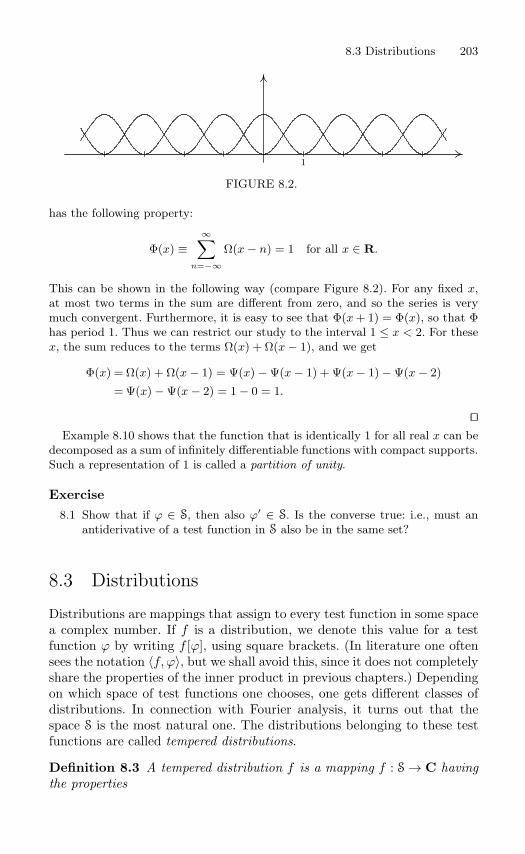
8.3 Distributions 203
1
FIGURE 8.2.
has the following property:
Φ(x) ≡∞∑
n=−∞Ω(x− n) = 1 for all x ∈ R.
This can be shown in the following way (compare Figure 8.2). For any fixed x,at most two terms in the sum are different from zero, and so the series is verymuch convergent. Furthermore, it is easy to see that Φ(x+ 1) = Φ(x), so that Φhas period 1. Thus we can restrict our study to the interval 1 ≤ x < 2. For thesex, the sum reduces to the terms Ω(x) + Ω(x− 1), and we get
Φ(x) = Ω(x) + Ω(x− 1) = Ψ(x) − Ψ(x− 1) + Ψ(x− 1) − Ψ(x− 2)
= Ψ(x) − Ψ(x− 2) = 1 − 0 = 1.
Example 8.10 shows that the function that is identically 1 for all real x can be
decomposed as a sum of infinitely differentiable functions with compact supports.Such a representation of 1 is called a partition of unity.
Exercise
8.1 Show that if ϕ ∈ S, then also ϕ′ ∈ S. Is the converse true: i.e., must anantiderivative of a test function in S also be in the same set?
8.3 Distributions
Distributions are mappings that assign to every test function in some spacea complex number. If f is a distribution, we denote this value for a testfunction ϕ by writing f [ϕ], using square brackets. (In literature one oftensees the notation 〈f, ϕ〉, but we shall avoid this, since it does not completelyshare the properties of the inner product in previous chapters.) Dependingon which space of test functions one chooses, one gets different classes ofdistributions. In connection with Fourier analysis, it turns out that thespace S is the most natural one. The distributions belonging to these testfunctions are called tempered distributions.
Definition 8.3 A tempered distribution f is a mapping f : S → C havingthe properties

204 8. Distributions
(1) linearity: f [c1ϕ1 + c2ϕ2] = c1f [ϕ1] + c2f [ϕ2] for all ϕk ∈ S and scalarsck;
(2) continuity: if ϕjS−→ ψ as j → ∞, then also lim
j→∞f [ϕj ] = f [ψ].
The set of all tempered distributions is denoted S′.
We give some examples.
Example 8.11. Let f be a continuous function on R such that there areconstants M and m such that |f(x)| ≤ M(1 + |x|)m for all x. Then we candefine a tempered distribution Tf by letting
Tf [ϕ] =∫Rf(x)ϕ(x) dx.
It is clear that Tf is a linear mapping; the fact that it is continuous followsfrom the fact that convergence in S implies uniform convergence even aftermultiplication by expressions such as (1 + |x|)m+2:
|Tf [ϕj ] − Tf [ψ]| =∣∣∣∣∫
Rf(x)(ϕj(x) − ψ(x)) dx
∣∣∣∣≤∫RM(1 + |x|)m|ϕj(x) − ψ(x)| dx
=∫RM(1 + |x|)m+2|ϕj(x) − ψ(x)| · dx
(1 + |x|)2
≤M maxx∈R
(1 + |x|)m+2|ϕj(x) − ψ(x)| ·
∫R
dx
(1 + |x|)2 → 0
as j → ∞. It is customary to identify the distribution Tf with the functionf and write f [ϕ] instead of Tf [ϕ]. In this way, every continuous, moderatelyincreasing function can be considered to be a distribution, and it is in thisway that distributions can be seen as generalizations of ordinary functions.
It is not necessary that the f in Example 8.11 be continuous. It is suffi-
cient that it is locally integrable, i.e., that∫ b
a|f(x)| dx exists and is finite for
all compact intervals [a, b]; on the other hand, it cannot be allowed to growtoo fast as |x| → ∞. An important distribution of this type is exhibited inthe next example:
Example 8.12. Let H be the Heaviside function, defined by
H(x) = 0 if x < 0, H(x) = 1 if x > 0.
(The value ofH(0) is immaterial.) This defines a distribution by the formula
H[ϕ] =∫RH(x)ϕ(x) dx =
∫ ∞
0ϕ(x) dx.

8.3 Distributions 205
Example 8.13. Define δ ∈ S′ by δ[ϕ] = ϕ(0). (The reader is asked tocheck linearity and continuity.) This distribution is called the Dirac distri-bution (Dirac function, Dirac measure), and this is the object announcedin Examples 8.2 and 8.3.
If f is an arbitrary distribution, as a rule there exists no “value at thepoint x” to be denoted by f(x). In spite of this, one often writes the effectof f on a test function ϕ as an integral:
f [ϕ] =∫Rf(x)ϕ(x) dx.
This is indeed a very symbolic notation, but, nevertheless, it turns outto be quite useful. The whole theory develops in such a way that thosesuggestions that are invoked by the integral symbolism will be “correct.”As an example, one writes
ϕ(0) = δ[ϕ] =∫Rδ(x)ϕ(x) dx.
If we symbolically translate the δ function and write δ(x−a), the ordinaryrules for changing variables yield∫
Rδ(x− a)ϕ(x) dx =
∫Rδ(y)ϕ(y + a) dy =
[ϕ(y + a)
]y=0 = ϕ(a).
One often writes δa(x) = δ(x − a), so that δa is the distribution given byδa[ϕ] = ϕ(a).
We include another few very mixed examples.
Example 8.14. The mapping f that is defined by
f [ϕ] = 3ϕ(2) − 4ϕ′(2) + 7ϕ(8)(π) +∫ 3
2ϕ′′(x) cos 7x dx
is a tempered distribution. Example 8.15. The function 1/x cannot play the role of f in Exam-ple 8.11, since the integral will be divergent at the origin, However, we candefine f [ϕ] using a symmetric limit:
f [ϕ] = limε0
∫|x|>ε
ϕ(x)x
dx = limε0
(∫ −ε
−∞+∫ ∞
ε
)ϕ(x)x
dx
= limε0
∫ ∞
ε
ϕ(x) − ϕ(−x)x
dx.
The integral converges because the integrand in the last version has a finitelimit as x 0, namely, 2ϕ′(0). It is not difficult to prove that the formula

206 8. Distributions
actually defines a tempered distribution. This distribution is commonlycalled P.V.1/x, where P.V. stands for principal value, which means thesymmetric limit in the formula.
Example 8.16. If f(x) = ex2, then f does not describe a tempered dis-
tribution according to Example 8.11. Indeed, if we choose the test functionϕ(x) = e−x2
, which clearly belongs to S, the integral will diverge. Thefunction f increases too fast.
Remark. If, instead of S, one starts with the test function sets D or E (with suit-able definitions of convergence, which are omitted here), one obtains other classesof distributions. Starting from D, consisting of test functions with compact sup-port, one gets the class D′ of, simply, distributions. These comprise the tempereddistributions as a subset, but also lots of others. For example, the function f inExample 8.16 defines such a general distribution.
If one starts with E — i.e., all C∞ functions are included among the testfunctions — one gets a more restricted set E′, consisting of all distributions withcompact support, which is defined in the next section.
Exercises
8.2 Show that f(x) = ln |x| defines a distribution according to Example 8.11.(What has to be proved is essentially that f is locally integrable.)
8.3 Which of the following formulae define elements of S′?
(a) f [ϕ] =∫R
(2x2 + 3)ϕ′′(x) dx, (b) f [ϕ] =∫R
exϕ(x) dx,
(c) f [ϕ] = (ϕ(0))2.
8.4 Properties
We are going to introduce some fundamental notions describing variousproperties of tempered distributions. (In the interest of brevity, we shallmostly omit the word “tempered.”)
Two distributions f and g are equal (or globally equal), if f [ϕ] = g[ϕ]for all ϕ ∈ S.
For f, g ∈ S′, the sum f + g is defined by (f + g)[ϕ] = f [ϕ] + g[ϕ] for allϕ ∈ S. If c is a scalar (a complex number), then cf is the distribution thatis described by (cf)[ϕ] = c · f [ϕ]. With these operations, S′ itself becomesa linear space.
A distribution f is zero on an open interval I =]a, b[, if f [ϕ] = 0 for allϕ ∈ S that have suppϕ ⊂ I. Two distributions f and g are equal on anopen interval I if f − g is zero on I. For example, δ = 0 on the interval]0,∞[.

8.4 Properties 207
If f and g are ordinary functions, equality on I means that f(x) = g(x)for all x ∈ I except possibly for a set of measure zero (a zero set, cf. page89). Just as in Chapter 5, we consider such functions to be equivalent (or,loosely speaking, to be the same).
The support supp f of a distribution f should be the smallest closed setwhere, loosely speaking, it really does matter what values are taken by thetest functions; more precisely, a point x does not belong to the support ifthere is a neighborhood (an open interval) around x where f is zero. Thesupport is always a closed set.
Example 8.17. For a distribution that is a continuous function, f [ϕ] =∫R fϕ dx, the support of f as a distribution coincides with the support off as a function. If f is discontinuous, the expression “f is zero” in thedefinition above should be changed to “f is zero except possibly for a setof measure zero”. Example 8.18. With the notation of Sec. 8.3, suppH = [0,∞[, supp δ =0, supp δa = a. The support of the distribution in Example 8.14 is theset [2, 3] ∪ π.
If χ is a multiplicator function and f ∈ S′, we can define the productχf ∈ S′ by putting (χf)[ϕ] = f [χϕ] for all ϕ ∈ S. (Check that this isreasonable if f is an ordinary function, and that χf actually turns out tobe a tempered distribution!)
Example 8.19. What is the product χδ ? According to the definition wehave
(χδ)[ϕ] = δ[χϕ] = χ(0)ϕ(0) = χ(0) · δ[ϕ].
This result is often written in the form
χ(x)δ(x) = χ(0)δ(x).
In the same way one sees that in general
χ(x)δ(x− a) = χ(a)δ(x− a). (8.1)
Example 8.20. Let f be P.V.1/x, and χ(x) = x. What is χf ? Indeed,
χf [ϕ] = f [χϕ] = limε0
∫|x|>ε
x · ϕ(x)x
dx = limε0
∫|x|>ε
ϕ(x) dx
=∫ ∞
−∞ϕ(x) dx =
∫R
1 · ϕ(x) dx.
We see that χf can be identified with the function which is identically 1,which we write simply as x · P.V.1/x = 1.

208 8. Distributions
Now, at last, we arrive at the promised generalization of the notion of aderivative. The starting point is the formula for integration by parts:∫ b
a
f ′(x)ϕ(x) dx = f(b)ϕ(b) − f(a)ϕ(a) −∫ b
a
f(x)ϕ′(x) dx.
If f is a moderately increasing function of class C1, and ϕ ∈ S, we can leta → −∞ and b → ∞. The contributions at a and b will both tend to zero,and we are left with∫
Rf ′(x)ϕ(x) dx = −
∫Rf(x)ϕ′(x) dx.
This inspires the following definition:
Definition 8.4 If f ∈ S′, a new tempered distribution f ′ is defined by
f ′[ϕ] = −f [ϕ′] for all ϕ ∈ S.
We call f ′ the derivative of f .
It is not hard to check that actually f ′ ∈ S′; here we profit from therigorous conditions that we have placed upon our test functions! Let usinvestigate some common cases. If f ∈ C1(R), the new derivative will coin-cide with the old one. But now, functions that did not have a derivative inthe traditional sense will find themselves to have one, this being a distribu-tion rather than an ordinary function. Also, the definition of the derivativecan be iterated any number of times, and we find that all f ∈ S′ suddenlyare endowed with derivatives of all orders!
Example 8.21. Find the derivative of the Heaviside function H ! Bydefinition, it should emerge from the following calculation:
H ′[ϕ] = −H[ϕ′] = −∫ ∞
0ϕ′(x) dx = −[ϕ(x)
]∞x=0 = −(0 − ϕ(0))
= ϕ(0) = δ[ϕ].
We see that H ′ = δ, the derivative of the Heaviside function is the Dirac“function.” The latter is commonly illustrated graphically by a “spike” (seeFigure 8.3). In general, it can be seen that the derivative of a jump of sizec at a point x = a is given by cδa (or cδ(x− a) ).
Example 8.22. Find the derivatives of δ:
δ′[ϕ] = −δ[ϕ′] = −ϕ′(0), δ′′[ϕ] = −δ′[ϕ′] = δ[ϕ′′] = ϕ′′(0).
In general, δ(n)[ϕ] = (−1)n ϕ(n)(0).

8.4 Properties 209
2δ−2
δ
− 32δ3
0 1x
FIGURE 8.3.
Example 8.23. What is the derivative of χf , where χ belongs to M andf ∈ S′ ? On the one hand,
(χf)′[ϕ] = −(χf)[ϕ′] = −f [χϕ′],
and on the other,
(χ′f + χf ′)[ϕ] = (χ′f)[ϕ] + (χf ′)[ϕ] = f [χ′ϕ] + f ′[χϕ]= f [χ′ϕ] − f [(χϕ)′] = f [χ′ϕ] − f [χ′ϕ+ χϕ′] = −f [χϕ′].
(Give some thought to what motivates each individual equality sign in thesecalculations!) One can see that the distributions (χf)′ and χ′f + χf ′ havethe same effect on arbitrary test functions; thus we have proved the rule
(χf)′ = χ′f + χf ′ if χ is moderately increasing and f ∈ S′.
In calculations involving functions that are defined by different formulae
in different intervals, it is practical to make use of translated Heavisidefunctions. If a < b, the expression H(t − a) − H(t − b) is equal to 1 fora < t < b and equal to 0 outside the interval [a, b]. It might be called a“window” that lights up the interval (a, b) (we do not in these situationscare much about whether an interval is open or closed). For unboundedintervals we can also find “windows”: the function H(t − a) lights up theinterval (a,∞), and the expression 1 −H(t− b) the interval (−∞, b).
Example 8.24. Consider the function f : R → R that is given by
f(t) =
1 − t2 for t < −2,t+ 2 for − 2 < t < 1,1 − t for t > 1.
210 8. Distributions
This can now be compressed into one formula:
f(t) = (1 − t2)(1 −H(t+ 2)) + (t+ 2)(H(t+ 2) −H(t− 1))+(1 − t)H(t− 1)
= (1 − t2) + (−1 + t2 + t+ 2)H(t+ 2) + (−t− 2 + 1 − t)H(t− 1)= 1 − t2 + (t2 + t+ 1)H(t+ 2) − (2t+ 1)H(t− 1).
Example 8.25. The function f(x) = |x2 − 1| can be rewritten as
f(x) = (x2 − 1)H(x− 1) + (1 − x2)(H(x+ 1) −H(x− 1))+(x2 − 1)(1 −H(x+ 1))
= (x2 − 1)(2H(x− 1) − 2H(x+ 1) + 1
).
This formula can be differentiated, using the rule for differentiating a prod-uct:
f ′(x) = 2x(2H(x− 1) − 2H(x+ 1) + 1
)+ (x2 − 1)
(2δ(x− 1) − 2δ(x+ 1)
)= 2x
(2H(x− 1) − 2H(x+ 1) + 1
).
In the last step, we used the formula (8.1). One more differentiation gives
f ′′(x) = 2(2H(x− 1) − 2H(x+ 1) + 1
)+ 2x
(2δ(x− 1) − 2δ(x+ 1)
)= 2
(2H(x− 1) − 2H(x+ 1) + 1
)+ 4δ(x− 1) + 4δ(x+ 1).
The first term contains the classical second derivative of |x2 − 1|, whichexists for x = ±1; the two δ terms demonstrate that f ′ has upward jumpsof size 4 for x = ±1. See Figure 8.4.
Example 8.26. Let a > 0 and b be real constants. If f ∈ S′, define g byg(x) = f(ax+ b). This means that (using symbolic integrals)
g[ϕ] =∫f(ax+b)ϕ(x) dx =
∫f(y)ϕ
(y − b
a
)dy
a=∫f(x)ϕ
(x− b
a
)dx
a,
(8.2)i.e.,
g[ϕ] =1af
[x → ϕ
(x− b
a
)].
What connection holds between the derivatives of f and g ? By the defini-tion of g′ we should have
g′[ϕ] = −g[ϕ′] = −∫f(ax+ b)ϕ′(x) dx.

8.4 Properties 211
1
1
f
1
2
f ′
1
2
f ′′
FIGURE 8.4.
What is the effect of the distribution h that is symbolically written h(x) =af ′(ax+ b) ? Well, using the same change of variable as in (8.2) we get
h[ϕ] = a
∫f ′(ax+ b)ϕ(x) dx = a
∫f ′(x)ϕ
(x− b
a
)dx
a
=∫f ′(x)ϕ
(x− b
a
)dx,
and the definition of f ′ then yields
h[ϕ] = −∫f(x)
d
dxϕ
(x− b
a
)dx = −1
a
∫f(x)ϕ′
(x− b
a
)dx,
which, after a change of variable, proves to be − ∫f(ax + b)ϕ′(x) dx. If
a < 0, the computations are analogous (there will occur a couple of minussigns that cancel in the end). We have then proved that the formula g′(x) =af ′(ax + b) holds even for distributions. (In fact, the chain rule will holdalso for more general changes of variable than these, but we will not delvedeeper into this. Too “general” changes of variable may lead us out of thespaces S and S′ where we have chosen to stay in this exposition.)
Using the new notion of derivative, we have now a solution of the oldtrouble with the wave equation, c2uxx = utt. If we let f and g be twofunctions on R and form
u(x, t) = f(x− ct) + g(x+ ct),
we can take derivatives of f and g in the distribution sense. Using the chainrule as in Example 8.26 it is seen immediately that u satisfies the equation.
In what follows we shall need the following result.

212 8. Distributions
Theorem 8.1 If f ∈ S′, then f ′ = 0 if and only if f is a constant function.
To prove the theorem we need a lemma.
Lemma 8.2 A test function ϕ ∈ S is the derivative of another function inS if and only if
∫R ϕ(x) dx = 0.
Clearly, if ϕ = Φ′, then∫ϕ = Φ(∞) − Φ(−∞) = 0, so the hard part
is to prove the converse statement. If∫ϕ = 0, we can define a primitive
function Φ by
Φ(x) =∫ x
−∞ϕ(y) dy = −
∫ ∞
x
ϕ(y) dy.
Obviously, Φ is infinitely differentiable, for Φ(k) = ϕ(k−1), and estimates ofthese derivatives are no problem. What remains is to show that the functionitself tends to zero quickly enough. However, if n is an integer, we do knowthat |ϕ(y)| ≤ C/(1 + |y|)n+2 for some C, and for x ≥ 0 we then have
(1 + |x|)n|Φ(x)| ≤ (1 + |x|)n
∫ ∞
x
C dy
(1 + |y|)n+2
≤ (1 + |x|)n
(1 + |x|)n
∫ ∞
x
C dy
(1 + |y|)2 ≤ C1.
For x < 0, we can do the analogous thing to the other one of the integralsthat define Φ. This shows that Φ ∈ S′, and the lemma is proved.
Proof of Theorem 8.1. Saying that f is the constant c means that f isidentified with the differentiable function f(x) = c; in this case, the newderivative coincides with the traditional one, so that f ′ = 0. The converseis harder. Assume that f ′ = 0. Then
f [ϕ′] = −f ′[ϕ] = 0 for all ϕ ∈ S. (8.3)
However, we must know what f ′ does to an arbitrary test function. Let ψ0be a fixed test function such that
∫ψ0(x) dx = 1. For an arbitrary ϕ ∈ S,
put A =∫ϕ(x) dx. Then ϕ − Aψ0 is a test function with integral 0, and
by the lemma it is the derivative of some function belonging to S. Putc = f [ψ0]. Using (8.3) we find that
0 = f [ϕ−Aψ0] = f [ϕ] −Af [ψ0] = f [ϕ] −∫ϕ(x) dx · f [ψ0]
= f [ϕ] − c
∫ϕ(x) dx,
and it follows that f [ϕ] =∫cϕ(x) dx, which means that f can be identified
with the constant c. Let fj ∈ S′ for j = 1, 2, 3, . . .. Suppose that g ∈ S′ has the property
that limj→∞ fj [ϕ] = g[ϕ] for all ϕ ∈ S. Then we say that the sequence

8.5 Fourier transformation 213
fj converges in S′ to g, which we write as fj → g or, when precision is
needed, fjS′
−→ g. This sort of convergence is clearly simple and natural. Animmediate consequence is that every positive summation kernel (Sec. 2.4)converges to the Dirac distribution.
Remark. A curious reader is probably missing one operation among the defi-nitions that we have made: multiplication. It turns out, however, that it is notpossible to define the product of two distributions in general. It is possible tomultiply certain couples, but other products cannot be given a meaningful inter-pretation. In this text we have treated a simple case: the product of a so-calledmultiplicator function and a distribution. This case will be sufficient for ourpresent needs.
Exercises8.4 Show that x2δ′′′ = 6δ′.
8.5 Prove the following formula: χ(x)δ′(x−a) = χ(a)δ′(x−a)−χ′(a)δ(x−a).
8.6 Find the third derivative of |x3 − x2 − x+ 1|.8.7 Show that the distributional derivative of ln |x| is P.V.(1/x).
8.8 Show that the derivative of f = P.V.(1/x) is described by the formula
f ′[ϕ] = − limε0
∫|x|≥ε
ϕ(x) − ϕ(0)x2 dx.
8.9 Consider Exercise 2.20, page 25. Interpret this exercise as a result in distri-bution theory. Sketch the graph of the “kernel” occurring in the problem.
8.5 Fourier transformation
If ϕ ∈ S, it is certainly true that ϕ ∈ L1(R), and in addition ϕ(k) ∈L1(R) for all k ≥ 1. This means that ϕ and all its derivatives have Fouriertransforms:
ϕ(k)(ω) =∫Rϕ(k)(x) e−iωx dx.
Integrating by parts and using the fact that ϕ(m)(x) decreases rapidly asx → ±∞, one can see that
ϕ(k)(ω) = (−1)k
∫Rϕ(x)Dk
x
(e−iωx
)dx = (iω)k ϕ(ω).
Since the transform of ϕ(k) is bounded (Theorem 7.1), it follows that|ω|k|ϕ(ω)| ≤ Ck, i.e., ϕ decreases at least as fast as 1/|ω|k at infinity;and this is true for all k ≥ 0. Furthermore, we can form the derivative ofϕ:
dn
dωnϕ(ω) =
∫Rϕ(x) (−ix)n e−iωx dx,

214 8. Distributions
where differentiation under the integral sign is allowed because the resultingintegral converges uniformly (again we use that ϕ(x) is small when |x| islarge). Thus, ϕ ∈ C∞. But on the last integral we can again apply thesame procedure as above to see that the derivatives also decrease rapidlyas ω → ±∞. Collecting our results, we have proved part of the followingtheorem.
Theorem 8.2 The Fourier transformation F is a continuous bijection ofthe space S onto itself.
In plain words: if ϕ ∈ S on the x-axis, then F(ϕ) = ϕ ∈ S on the ω-axis,and every function ψ(ω) belonging to S is the Fourier transform of somefunction ϕ ∈ S. The latter statement follows from the fact that if ψ(ω)belongs to S, then one can form the inverse Fourier transform ϕ of ψ:
ϕ(x) =12π
∫Rψ(ω) eixω dω. (8.4)
Just as in the argument before the theorem, one sees that ϕ will be amember of S on the x-axis and that the Fourier inversion formula givesthat ϕ = ψ.
The fact that the Fourier transformation is a continuous mapping fromS to S means that if ϕj
S−→ ψ, then also ϕjS−→ ψ. We omit the details of
the proof of this fact; essentially it hinges on the fact that the expressions
maxω∈R
(1 + |ω|)n|ϕj(k)(ω) − ψ(k)(ω)|
can be estimated by the corresponding expressions for (1+|x|)k|ϕ(n)j −ψ(n)|.
(Roughly speaking, differentiation on one side corresponds to multiplicationby the variable on the other side.)
Again we stress that if ϕ ∈ S, then the Fourier inversion formula (8.4)will always hold. There are no convergence problems for the integral, sinceϕ(ω) tends rapidly to zero at both infinities. The definition of S is tailoredso that the Fourier transformation shall have all these nice properties.
Now we want to define the Fourier transform of a distribution. As apreparation, we do a “classical” calculation. Assume that f(x) and g(ω)are functions belonging to L1, each on its own axis:
‖f‖1 =∫R
|f(x)| dx < ∞, ‖g‖1 =∫R
|g(ω)| dω < ∞.
The Fourier transforms f and g both exist:
f(ω) =∫Rf(x) e−iωx dx, g(x) =
∫Rg(ω) e−ixω dω,
and they satisfy the inequalities |f(ω)| ≤ ‖f‖1 and |g(x)| ≤ ‖g‖1. Thefunction f(x) g(ω) e−ixω will then be absolutely integrable over the plane
8.5 Fourier transformation 215
R × R, and the integral can be computed by iteration in two ways. Thisgives the identity∫∫
R×R
f(x) g(ω) e−ixω dx dω =∫Rf(x) g(x) dx =
∫Rf(ω) g(ω) dω.
The equality of the two last members is our inspiration. It is, for example,true if g = ϕ ∈ S and f is any L1 function. We extend its domain of validityin the following definition.
Definition 8.5 The Fourier transform of f ∈ S′ is the distribution f thatis defined by the formula
f [ϕ] = f [ϕ] for all ϕ ∈ S.
Just as in Chapter 7, we shall also write f = F(f) (but now we useordinary brackets instead of square ones, in order to avoid confusing itwith the notation f [ϕ]).
Remark. The equality∫fg =
∫fg is sometimes considered to be a variant of
the polarized version of the Plancherel formula. We proceed to check that f is actually a tempered distribution. It is clear
that it is linear:
f [c1ϕ1 + c2ϕ2] = f[(c1ϕ1 + c2ϕ2)∧] = f [c1ϕ1 + c2ϕ2]
= c1f [ϕ1] + c2[ϕ2] = c1f [ϕ1] + c2f [ϕ2].
The continuity is a simple consequence of the continuity of the Fouriertransformation on S: if ϕj
S−→ ψ, then
f [ϕj ] = f [ϕj ] → f [ψ] = f [ψ],
which tells us precisely that f is continuous, and thus a distribution.Let us compute the Fourier transforms of some distributions. We start
with a few examples that are ordinary functions, but do not belong toL1(R).
Example 8.27. Let f(x) = 1 for all x. What is the Fourier transform f ?We should have
f [ϕ] = f [ϕ] =∫Rf(x) ϕ(x) dx =
∫Rϕ(x) dx
= 2π · 12π
∫Rϕ(x) ei0x dx = 2πϕ(0) = 2πδ[ϕ].
It follows that f = 2π δ, or f(ω) = 2π δ(ω) if we want to stress the name ofthe independent variable. (Notice that the test functions and their trans-forms have reversed independent variables in this connection!)

216 8. Distributions
Example 8.28. Take f(x) = xn (n integer ≥ 0). This function defines atempered distribution, and its transform satisfies
f [ϕ] = f [ϕ] =∫Rxn ϕ(x) dx.
By the ordinary rules for Fourier transforms we have that (ix)n ϕ(x) is thetransform of the function ϕ(n), which means that xn ϕ(x) is the transformof (−i)n ϕ(n). The inversion formula then gives that f [ϕ] = 2π(−i)nϕ(n)(0).In the preceding section we saw that the nth derivative of δ is describedby δ(n)[ϕ] = (−1)nϕ(n)(0). Thus we must have f = 2πinδ(n).
Before giving further examples we present a list of rules of computation,which on the face look quite familiar, but now are in need of new proofs. Tosimplify the formulation, we introduce two new notations. First, if f ∈ S′,then f is what could be symbolically written as f(−x); more precisely,we define f [ϕ] =
∫f(x)ϕ(−x) dx. We say that f is even if f = f , odd if
f = −f .Secondly, if a ∈ R and ϕ ∈ S, we define the translated function ϕa by
ϕa(x) = ϕ(x − a). For f ∈ S′ the translated distribution fa is f(x − a),which means fa[ϕ] =
∫f(x)ϕ(x + a) dx = f [ϕ−a]. (This notation is a
generalization of the notation δa to arbitary distributions.)
Theorem 8.3 If f, g ∈ S′, then
(a) f is even/odd ⇐⇒ f is even/odd.
(b) f=2πf .
(c) fa = e−iaω f .
(d) F(eiaxf) =(f)a.
(e) f ′ = iωf .
(f) xf = i(f)′.
Proving these formulae are excellent exercises in the definitions of thenotions involved. As examples, we perform the proofs of rules (d) and (e):
(d): The effect of the left-hand member on a test function ϕ is rewritten:
F(eiaxf)[ϕ] = (eiaxf)[ϕ] = f [eiaxϕ] = f [F(ϕ−a)] = f [ϕ−a] = (f)a[ϕ].
Each equality sign corresponds to a definition or a theorem: the first oneis the definition of the Fourier transform; the second one is the definitionof the product of a function and a distribution; the third one is a rulefor “classical” Fourier transforms; the fourth is again the definition of theFourier transform; and the last one is the definition of the translate of adistribution.

8.5 Fourier transformation 217
(e) is proved similarly; the reader is asked to identify the reason for eachequality sign in the following formula:
f ′[ϕ] = f ′[ϕ] = −f [(ϕ)′] = −f [F(−iωϕ)] = f [F(iωϕ)] = f [iωϕ]
= (iωf)[ϕ].
We proceed to give more examples of transforms of distributions.
Example 8.29. Transform f = P.V.1/x (Example 8.15, page 205): wehave seen that xf = 1. Transformation gives iDf = 2πδ = 2πH ′, whichcan be rewritten as iD(f + 2πiH) = 0. By Theorem 8.1 it follows thatf+2πiH = c = constant, whence f = c−2πiH. To determine the constantwe notice that f is odd, and thus f must also be odd. This gives c = πiand f = πi(1 − 2H).
If we introduce the function sgnx = x/|x| (the sign of x), we can writethe result as f = −πi sgnx. Example 8.30. H = the Heaviside function. In Example 8.29 we saw that
F(P.V.1x
)(ω) = πi(1 − 2H(ω)).
Since both sides are odd distributions, rule (b) gives
πiF(1 − 2H)(ω) = 2π(
P.V.1ω
)∨= −2πP.V.
1ω.
On the other hand, F(1 − 2H) = 1 − 2H = 2πδ − 2H. From this we cansolve
H = πδ(ω) − iP.V.1ω.
As a finale to this section we prove the following result.
Theorem 8.4 If f ∈ S′, then xf(x) is the zero distribution if and only iff = Aδ for some constant A.
Proof. Transformation of the equation xf(x) = 0 gives if ′ = 0, and byTheorem 8.1 this means that f = C, where C is a constant. Transformback again: since 1 = 2πδ, we find that f must be a constant times δ, andthe proof is complete.
By translation of the situation in the theorem, it is seen that the followingalso holds: if f ∈ S′ and (x− a)f(x) = 0, then f = Aδa for some constantA. This can be further generalized. If χ is a multiplicator function that hasa simple zero at the point x = a, and χf = 0, then f = Aδa. The proof is
218 8. Distributions
built on writing χ(x) = (x−a)ψ(x), where ψ(a) = 0, and then the previousresult is applied to the distribution ψf .
A different kind of generalization of Theorem 8.4 is given in Exercise 8.14.
Exercises
8.10 Determine the Fourier transform of f(x) = e−xH(x). What is the transformof 1/(1 + ix) ? Of x/(1 − ix) ?
8.11 Let f1 = P.V.1/x. Define recursively fn for n = 2, 3, . . . by fn+1 = −f ′n/n.
Prove that xnfn = 1 for n = 1, 2, 3, . . ..
8.12 Find the Fourier transform of x3/(1 + x2) .
8.13 Find a tempered distribution f that solves the integral equation∫ ∞
0
e−uf(t− u) du = H(t), −∞ < t < ∞, t = 0.
Check your result by substituting into the equation.
8.14 Suppose that f ∈ S′ is such that xnf = 0 for an integer n. Prove that f isa linear combination of δ(k), k = 0, 1, . . . , n− 1.
8.15 Let f be a function of moderate growth on R such that
f(x) =12
∫ 1
−1
f(x− t) dt for all x ∈ R.
(That is, f(x) is always equal to its mean value over the interval of length2 with x in its middle.) Prove that f must be a polynomial of degree atmost 1. (Hint: take Fourier transforms and use the result of the precedingexercise.)
8.6 Convolution
Two test functions in S can always be convolved according to the recipe inSec. 7.5, because the defining integral
f ∗ g(x) =∫Rf(x− y)g(y) dy =
∫Rf(y)g(x− y) dy
converges very nicely. But the operation of convolution can be extended tomore general situations. If one of the functions is continuous and bounded,and the other one belongs to L1(R), it works nicely, too. Now we shall takeone of them to be a distribution and the other one a test function: thus letf ∈ S′ and ϕ ∈ S. By the convolution of f and ϕ we mean the function f ∗ϕgiven by f ∗ ϕ(x) = f [ϕx] = fy[ϕ(x − y)], where the subscript y indicatesthat the distribution acts with respect to the variable y. With a symbolicintegral: f ∗ ϕ(x) =
∫f(y)ϕ(x− y) dy.
8.6 Convolution 219
The convolution is thus an ordinary function of the variable x. One canalso prove that it is infinitely differentiable. This follows from the fact thatfor each fixed x, the sequence of functions ψh, defined by
y → ψh(y) =ϕ(x+ h− y) − ϕ(x− y)
h,
will converge in the sense of S, as h → 0 (with the function y → ϕ′(x− y)as the limit). (The verification of this statement is somewhat complicated;it involves the notion of uniform continuity.) This implies that
f ∗ ϕ(x+ h) − f ∗ ϕ(x)h
=fy[ϕ(x+ h− y)] − fy[ϕ(x− y)]
h= f [ψh]
→ fy[ϕ′(x− y)] = f ∗ ϕ′(x).
The reasoning can be iterated, and one finds that f ∗ ϕ has derivatives ofall orders, that also satisfy
Dn(f ∗ ϕ) = f ∗ ϕ(n).
What is the result of Fourier transforming a convolution of this type?The reader should be prepared for the answer. A proof of this runs alongthese lines: let ψ be an arbitrary test function:
ϕ ∗ f [ψ] = ϕ ∗ f [ψ] =∫ϕ ∗ f(x) ψ(x) dx =
∫∫ϕ(x− y) f(y) ψ(x) dx dy,
ϕ f [ψ] = f [ϕ ψ] = f [ϕψ] = f
[12π
ϕ ∗ ψ]
= f [ϕ ∗ ψ]
= fx[∫ ϕ(y − x)ψ(y) dy] =∫∫
f(x)ϕ(y − x) ψ(y) dx dy.
Since ϕ ∗ f and ϕf have the same effect on any test function, they arethe same distribution. (The proof may seem defective inasmuch as certainintegrals are “symbolic”, but this can be justified.)
The definition of convolution can be extended further by going a round-about way via the Fourier transform and the formula f ∗ g = F−1(f g), butfor this we refer to deeper texts.
The Dirac distribution δ has a special relation to the convolution oper-ation. As soon as the convolution is defined, one has δ ∗ f = f . Indeed, iff is continuous, we have
δ ∗ f(x) =∫δ(y)f(x− y) dy = [f(x− y)]y=0 = f(x).
Algebraically, this means that δ is a unit element for the operation ∗.
Exercises8.16 Compute the convolution δ(n) ∗ f , where f is a function belonging to E.8.17 Prove that f ∗ ϕ[ψ] = f [ϕ ∗ ψ], whenever f ∈ S and ϕ,ψ ∈ S′. (This could
be taken as an alternative definition of f ∗ ϕ.)

220 8. Distributions
−4π −2π 0 2π 4πx
FIGURE 8.5.
8.7 Periodic distributions and Fourier series
The intention of this section is to give just a hint about how distributiontheory actually can be used to unify the classical notions of Fourier seriesand Fourier transforms to make them special cases of one notion.
A tempered distribution f is said to be periodic with period 2P , if f [ϕ] =f [ϕ2P ] for all ϕ ∈ S or, symbolically,
∫f(x)ϕ(x) dx =
∫f(x)ϕ(x− 2P ) dx
for all ϕ ∈ S.
Example 8.31. A simple example of a distribution with period 2π is theso-called pulse train (see Figure 8.5):
X =∑n∈Z
δ2πn or X(x) =∑n∈Z
δ(x− n · 2π).
That this is actually a tempered distribution hinges essentially on the factthat the sum
X[ϕ] =∑n∈Z
ϕ(x+ n · 2π)
is convergent, which follows from the estimate |ϕ(x+n ·2π)| ≤ M/(1+n2),which is true for all ϕ ∈ S (with wide margins).
Let us investigate what the Fourier transform of a periodic distribution fshould look like. For simplicity, we assume that the period is 2π, so that wehave f2π = f . Direct transformation gives, using rule (c) in Theorem 8.3,
f = e−2πiω f ⇐⇒ (1 − e−2πiω)f = 0.
Evidently, for all ω such that e−2πiω = 1, f must be zero; this holds for allω = integer. At integer points ω = n, the factor 1 − e−2πiω has a simplezero, i.e., it behaves essentially like a nonzero constant times the factor(ω−n). Using Theorem 8.4 (in a “local” version) we see that f has a pointmass at ω = n, i.e., a multiple of δn. Thus we can write
f =∑n∈Z
γnδn or f(ω) =∑n∈Z
γnδ(ω − n)
for certain constants γn.

8.8 Fundamental solutions 221
In order to identify the coefficients γn, we consider the particular casewhen f is a “nice” 2π-periodic function. Then f has a nicely convergentordinary Fourier series, so that we can write
f(x) =∑n∈Z
cneinx, cn =
12π
∫ π
−π
f(x) e−inx dx.
If it is permissible to form the Fourier transform term by term, we coulduse the fact that the transform of eiαx is 2πδα, and we would get
f(ω) =∑n∈Z
cn · 2πδ(ω − n).
Thus it seems that the coefficients of the pulse train that makes up f arenothing but the classical Fourier coefficients of f (multiplied by the factor2π).
Formally, the inversion formula for the periodic distribution f would looklike this:
f(x) ∼ 12π
∫Rf(ω)eixω dω =
12π
∫R
∑n∈Z
cn · 2πδ(ω − n) eixω dω
=∑n∈Z
cnδn[eixω] =∑n∈Z
cneinx,
i.e., the inversion formula is the ordinary Fourier series.All these calculations can in fact be justified, and this is done in more
complete texts. It turns out that an arbitrary 2π-periodic distribution fhas a Fourier series/transform of the form
∑cne
inx and 2π∑cnδn, re-
spectively, where the coefficients satisfy an equality of the form |cn| ≤M(1 + |n|)k for some constants M and k; and, conversely, a pulse trainwith such coefficients is the Fourier transform of some periodic distribu-tion.
Exercise8.18 Find the Fourier transform of the pulse train X in Example 8.31.
8.8 Fundamental solutions
Let P (r) be a polynomial in the variable r, with constant coefficients. P (r)is the characteristic polynomial of the differential operator P (D), whichcan operate on functions or distributions:
P (r) = anrn + an−1r
n−1 + · · · + a1r + a0,
P (D) = anDn + an−1D
n−1 + · · · + a1D + a0,
P (D)y = any(n) + an−1y
(n−1) + · · · + a1y′ + a0y.
222 8. Distributions
For example, P (D) can be considered as a linear mapping S′ → S′.If P (D) operates on a convolution f ∗ ϕ, where, say, f ∈ S′ and ϕ ∈ S,
then the linearity and the rule for differentiation of a convolution implythat the result can be written
P (D)(f ∗ ϕ) = (P (D)f) ∗ ϕ = f ∗ (P (D)ϕ).
Now suppose that E ∈ S′ is a distribution such that P (D)E = δ, and letf be an arbitrary continuous function. Then we have
P (D)(E ∗ f) = (P (D)E) ∗ f = δ ∗ f = f.
Thus, if we have found such an E, we have a recipe for finding a particu-lar solution of the differential equation P (D)y = f , where the right-handmember f is an arbitrary (continuous) function. One says that E is a fun-damental solution of the operator P (D).
Example 8.32. Let a > 0. Let us find a fundamental solution of thefamiliar operator P (D) = D2 + a2, i.e., we want to find a distribution Esuch that E′′ + a2E = δ. Fourier transformation gives
(iω)2E + a2E = δ = 1,
and at least one solution of this ought to be found by solving for E likethis:
E =1
−ω2 + a2 =12a
(1
ω + a− 1ω − a
)=
i
4a
(2
i(ω + a)− 2i(ω − a)
).
(The two fractions in the last expression are interpreted as P.V.’s, as inExample 8.15.). We recognize that the Fourier transform of sgn t is 2/(iω),which gives
y(t) =i
4a(e−iatsgn t− eiatsgn t
)=
12a
sgn t sin at =12a
sin at · (2H(t) − 1).
Just to be safe, we check by differentiating:
y′(t) =12a
(a cos at(2H(t) − 1) + sin at · 2δ(t)) = 12 (cos at(2H(t) − 1)),
y′′(t) = 12 (−a sin at(2H(t) − 1) + cos at · 2δ(t))
= −a
2sin at · (2H(t) − 1) + δ(t) = −a2y(t) + δ(t).
Exercise8.19 Find fundamental solutions of the operators (a) P (D) = D−a, (b) P (D) =
D2 + 3D + 2, (c) P (D) = D2 + 2D + 1, (d) P (D) = D2 + 2D + 2.
8.9 Back to the starting point 223
8.9 Back to the starting point
We round off the chapter by looking back at the first section, 8.1, wherewe presented a number of “problems.” Most of these have now found somesort of solution.
Problem 8.1 was settled in Example 8.26: even an angular wave-shapehas derivatives in the distributional sense, and these derivatives satisfy thewave equation.
Problems 8.2–4 dealt with point charges of different kinds; the solution,as we have seen throughout the chapter, is to make the δ notion legitimateby viewing it as a distribution.
Problem 8.5 may be said to have been solved by the very idea of consid-ering distributions as linear functionals on a space of test functions.
There remains Problem 8.6. Let us first take the heat problem with theunknown function u = u(x, t):
uxx = ut, x ∈ R, t > 0; u(x, 0) = f(x), x ∈ R.
We can now let f be a tempered distribution on R. Assume that for everyfixed t, the thing that is symbolically denoted by x → u(x, t) is a tempereddistribution, and also assume that one can reverse the order of differen-tiation with respect to t and Fourier transformation with respect to x. Ifthe Fourier transform of u with respect to x is denoted by U(ω, t), as inSec. 7.7, we get the same transformed problem as we got there:
−ω2U =∂U
∂t, t > 0; U(ω, 0) = f .
This differential equation can be solved just as before, and we get U(ω, t) =e−ω2t · f , where the right-hand member is now a product of a test functionand a tempered distribution. Transforming back again we get u(x, t) =E(x, t) ∗ f , which is a convolution of a test function and a tempered dis-tribution, as in Sec. 8.6. An interesting fact is now that such a convolutionis actually an ordinary function, and furthermore this function has deriva-tives of all orders that actually satisfy the heat equation. The initial valuesare the distribution f in the sense that
u( · , t) S′−→ f as t 0.
The Dirichlet problem in the half-plane, which was considered in Sec. 7.8,can be treated in a similar way. A minor complication is the fact that thePoisson kernel
Py(x) =y
π
1y2 + x2
is not a test function, but the definition of convolution in Sec. 8.6 can beextended to encompass this case as well.
224 8. Distributions
Summary of Chapter 8
DefinitionWe say that a function ϕ belongs to the Schwartz class S if ϕ has derivativesof all orders and these satisfy inequalities of the form
(1 + |x|)n|ϕ(k)(x)| ≤ Cn,k, x ∈ R,
where Cn,k are constants for all integers n and k that are ≥ 0.
DefinitionA sequence ϕj∞
j=1 ⊂ S is said to converge in S to a function ψ ∈ S if forall integers n ≥ 0 and k ≥ 0 it holds that
limj→∞
maxx∈R
(1 + |x|)n|ϕ(k)j (x) − ψ(k)(x)| = 0.
DefinitionA tempered distribution f is a mapping f : S → C having the properties
(1) linearity: f [c1ϕ1 + c2ϕ2] = c1f [ϕ1] + c2f [ϕ2] for all ϕk ∈ S and scalarsck;
(2) continuity: if ϕjS−→ ψ as j → ∞, then also lim
j→∞f [ϕj ] = f [ψ].
The set of all tempered distributions is denoted by S′.Intuitively, a distribution on R is a sort of generalized function; it need
not have ordinary function values, but somehow it lives on the axis, andits “global” behavior is a sort of sum of its “local behavior”. For example,the Dirac distribution δ is zero everywhere except at the origin, where it isin a certain sense infinitely large.DefinitionIf f ∈ S′, a new tempered distribution f ′ is defined by
f ′[ϕ] = −f [ϕ′] for all ϕ ∈ S.
We call f ′ the derivative of f .
TheoremIf f ∈ S′, then f ′ = 0 if and only if f is a constant function.
TheoremThe Fourier transformation F is a continuous bijection of the space S ontoitself.

Historical notes 225
DefinitionThe Fourier transform of f ∈ S′ is the distribution f that is defined by theformula
f [ϕ] = f [ϕ] for all ϕ ∈ S.
If f ∈ S′, then f is what could be symbolically written as f(−x); moreprecisely, f [ϕ] =
∫f(x)ϕ(−x) dx. We say that f is even if f = f , odd if
f = −f .If a ∈ R and ϕ ∈ S, we define the translated function ϕa by ϕa(x) =
ϕ(x−a). For f ∈ S′ the translated distribution fa is f(x−a), which meansfa[ϕ] =
∫f(x)ϕ(x+ a) dx = f [ϕ−a].
TheoremIf f, g ∈ S′, then
(a) f is even/odd ⇐⇒ f is even/odd.
(b) f = 2πf .
(c) fa = e−iaω f .
(d) F(eiaxf) =(f)a.
(e) f ′ = iωf .
(f) xf = i(f)′.
Historical notes
The notion of a point mass was imagined already by Isaac Newton (1642–1727)in his description of the laws of gravity. Many physicists and applied mathe-maticians, such as Oliver Heaviside, in the nineteenth century, used this andanalogous concepts, with a varying sense of bad conscience, because they had nostringent mathematical formulation. Paul Dirac (1902–84), who won the No-bel Prize in Physics in 1933, discussed the problem closely and his name wasassociated to the object δ.
A mathematically acceptable definition of distributions was given around themiddle of the twentieth century by Laurent Schwarz (1915–2002). Simulta-neously, a number of Russian mathematicians developed a similar theory in aquite different way. They talked about generalized functions, defined as limits ofsequences of ordinary functions in a certain manner. It was soon discovered thatthe two definitions in fact give rise to equivalent notions.
The definitions are easily extended to several dimensions, so that one talksabout distributions on Rn. These objects have an enormous importance in thestudy of partial differential equations. There are also other sorts of generalizationsto even more general objects, such as hyperfunctions. Research in the field isintensive today.

226 8. Distributions
Problems for Chapter 8
If the star-marked sections in Chapters 2–7 have not been studied previously,the exercises there could now be looked up and solved. Here are another fewproblems.
8.20 Which of the following functions belong to S or/and M: e−x2, e−|x|5 ,
sin(x2), xn (n integer), 1/(1 + x2).
8.21 Decide which of these functions can be considered as distributions: e2x,e−2x, e2xH(x), e−2xH(x), esin x, (x2 − 1)3.
8.22 Find the first and second derivatives (in the sense of distributions) of(a) xH(x), (b) |x|, (c) |x2 − x|.
8.23 Simplify f(x) = ψ(x)δ′′(x− a), where ψ ∈ M.
8.24 Compute f ′′, where f(x) = | sinx|. Draw pictures of f , f ′, and f ′′.
8.25 An electric charge q at a point a on the x-axis can be represented byq δ(x − a). Suppose that we have one charge n at the point 1/n and anopposite charge −n at the point −1/n. The “limit” of this system, asn → ∞, is called an electric dipole. Describe this limit as a distribution!
8.26 Find all tempered distributions f satisfying the differential equationf ′(x) + 2xf(x) = δ(x− 2).
8.27 Determine the Fourier transforms of (a) sin ax, (b) cos bx,(c) xnH(x) (n = 0, 1, 2, . . .), (d) δ(x− a) + δ(x+ a), (e) xδ′(x).
8.28 Let a > 0. Find the Fourier transforms of e−axH(x) and eax(1−H(x)) andfinally of 1/(x+ bi), where b is a real number.
8.29 Find a solution in the form of a tempered distribution of the problemy′′ + a2y = δ. Then show how this distribution can be used to construct asolution of the equation y′′ + a2y = f , where f is an “arbitrary” function(i.e., a function belonging to some suitable class).

9Multi-dimensional Fourier analysis
In this chapter we give a sketch of what Fourier series and integrals look likein the multivariable case. There are almost no proofs. Sections 9.1–2 tackle theproblem of summing a series when the terms have no natural sequential order,which happens as soon as they are numbered in some other way than by indexsequences such as 1, 2, 3, . . . and similar sequences. In the next few sections weindicate what the Fourier analysis looks like. The intention behind these sectionsis to provide a sort of moral support for a student who comes across, say, in hisphysics studies, such things as Fourier transforms taken over all of 3-space – herea real mathematician is saying that these things do exist and can be used!
We have not included anything about distributions. This would have gone farbeyond the intended scope of this book. But the interested reader should knowthat distributions in Rn are an extremely useful tool, and the theory of theseobjects is both beautiful and exciting. Those who are interested should go on tosome of the books mentioned in the bibliography.
9.1 Rearranging series
In this section we presuppose that the reader is acquainted with the ele-ments of the theory of numerical series. By this we mean notions such asconvergence, absolute convergence, and comparison tests.
As is well known, if we want to compute the sum of finitely many terms,the order in which the terms are taken does not matter:
1 + 2 + 3 + 4 + 5 = 4 + 1 + 5 + 3 + 2.
228 9. Multi-dimensional Fourier analysis
This need not be the case when there are infinitely many terms, i.e., whenthe sum is a series.
Example 9.1. The series
∞∑k=1
(−1)k+1
k= 1 − 1
2 + 13 − 1
4 + 15 − 1
6 + · · ·
is convergent according to the so-called Leibniz test and has a certain sums > 1
2 (it can actually be shown that s = ln 2). If we rearrange the terms sothat each positive term is followed by two negative terms, so that we tryto sum
1 − 12 − 1
4 + 13 − 1
6 − 18 + 1
5 − 110 − 1
12 + 17 − 1
14 − 116 + · · · ,
it is rather easy to show that the partial sums now tend to s/2 = s. The reason things can be as bad as in the example is the following: If we
add those terms of the original series that are positive, which means thatwe write
1 + 13 + 1
5 + 17 + · · · + 1
2k−1 + · · · ,we get a divergent series; in like manner the negative terms also make upa divergent series:
− 12 − 1
4 − 16 − 1
8 − · · · − 12k − · · · .
This means that the sum of the original series is really an expression ofthe type “∞ − ∞”: there is an infinity of “positive mass” and an infinityof “negative mass.” Actually, it is not very difficult to describe a processthat can assign any given number as the sum of such a series, by taking theterms in a suitable order. It can also be made to diverge in various differentways. Se Exercise 9.1 below.
A convergent series∑∞
k=1 ak of this type, i.e., such that∑∞
k=1 |ak| isdivergent (= +∞, as it is often written), is said to be conditionally conver-gent. The alternative is an absolutely convergent series. For such a series thetroubles indicated above cannot happen. We are going to prove a theoremabout this. First we want to give a proper definition of a rearrangement ofa series. Let Z+ be the positive integers: Z+ = 1, 2, 3, . . ..
Definition 9.1 Let ϕ : Z+ → Z+ be a bijection, i.e., a one-to-one map-ping of the positive integers onto themselves. Then we say that the series∞∑
k=1
aϕ(k) is a rearrangement of the series∞∑
k=1
ak.
Theorem 9.1 An absolutely convergent series remains absolutely conver-gent and its sum does not change as a result of any rearrangement of itsterms.
9.1 Rearranging series 229
Proof. Put s =∑∞
k=1 ak. Let ϕ be a rearrangement bijection and puttn =
∑nk=1 aϕ(k). The starting point is that
∑ak is absolutely convergent,
i.e., that∞∑
k=1
|ak| = σ < +∞.
Let M(n) = max1≤k≤n ϕ(k). Then certainly
n∑k=1
|aϕ(k)| ≤M(n)∑j=1
|aj | ≤ σ < +∞,
and since σ does not depend on n it follows that the rearranged series isalso absolutely convergent. Now let ε > 0 be an arbitrary positive number.Then there exists an N0 = N0(ε) such that
∑∞j=N0+1 |aj | < ε. If m is large
enough, the numbers ϕ(1), ϕ(2), ϕ(3), . . . , ϕ(m) will surely include all thenumbers 1, 2, 3, . . . , N0 (and probably a lot of other numbers). Then we canestimate: for all sufficiently large values of m it holds that
|tm − s| =∣∣∣∣ m∑k=1
aϕ(k) −∞∑
j=1
ak
∣∣∣∣ =∣∣∣∣ ∑somej>N0
aj
∣∣∣∣ ≤∑somej>N0
|aj | ≤∞∑
j=N0+1
|aj | < ε,
which means that tm → s as m → ∞, and this is what we wanted to prove.
In certain situations it is natural to consider series with terms indexed byall integers: we have seen Fourier series in Chapter 4, and in complex anal-ysis one considers Laurent series. Such a series
∑k∈Z ak is (classically) con-
sidered as convergent if the two “halves”∑∞
k=0 ak and∑∞
k=1 a−k are bothseparately convergent. As we have seen in Chapter 4, there are also otherways to define the convergence of such a series. In the case of Fourier seriesit turns out to be natural to study the symmetric partial sums
∑nk=−n ak.
The example∞∑
k=−∞k
shows that these may well converge, although the series is divergent in theclassical sense.
Exercise9.1 (a) Describe (in principle) how to rearrange a conditionally convergent
series (for example the one in the introductory example above) to make itconverge to the sum 4.(b) Describe how to rearrange the same series so that it diverges to −∞.(c) The series can also be rearranged so that its partial sums make up asequence that is dense in the interval [−13, 2003]. How?(d) The partial sums can be dense on the whole real axis. How?
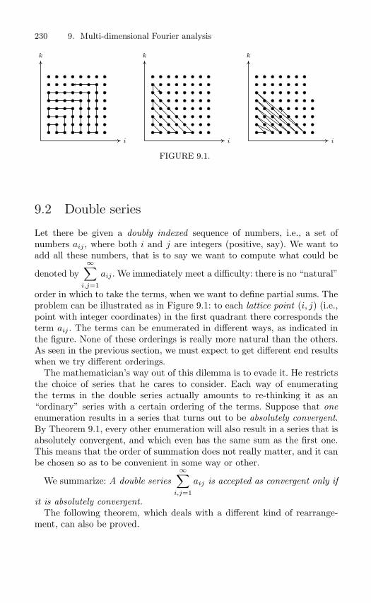
230 9. Multi-dimensional Fourier analysis
i
k
i
k
i
k
FIGURE 9.1.
9.2 Double series
Let there be given a doubly indexed sequence of numbers, i.e., a set ofnumbers aij , where both i and j are integers (positive, say). We want toadd all these numbers, that is to say we want to compute what could be
denoted by∞∑
i,j=1
aij . We immediately meet a difficulty: there is no “natural”
order in which to take the terms, when we want to define partial sums. Theproblem can be illustrated as in Figure 9.1: to each lattice point (i, j) (i.e.,point with integer coordinates) in the first quadrant there corresponds theterm aij . The terms can be enumerated in different ways, as indicated inthe figure. None of these orderings is really more natural than the others.As seen in the previous section, we must expect to get different end resultswhen we try different orderings.
The mathematician’s way out of this dilemma is to evade it. He restrictsthe choice of series that he cares to consider. Each way of enumeratingthe terms in the double series actually amounts to re-thinking it as an“ordinary” series with a certain ordering of the terms. Suppose that oneenumeration results in a series that turns out to be absolutely convergent.By Theorem 9.1, every other enumeration will also result in a series that isabsolutely convergent, and which even has the same sum as the first one.This means that the order of summation does not really matter, and it canbe chosen so as to be convenient in some way or other.
We summarize: A double series∞∑
i,j=1
aij is accepted as convergent only if
it is absolutely convergent.The following theorem, which deals with a different kind of rearrange-
ment, can also be proved.

9.2 Double series 231
Theorem 9.2 Suppose that the double series∞∑
i,j=1
aij is (absolutely) con-
vergent with sum s. Put
Vi =∞∑
j=1
aij , Hj =∞∑
i=1
aij .
Then also
s =∞∑
i=1
Vi =∞∑
j=1
Hj , (9.1)
where all the occurring series are also absolutely convergent.
In plain words, the formula (9.1) says that the series can be summed“first vertically and then horizontally,” or the other way round; (9.1) canbe written as
∞∑i,j=1
aij =∞∑
i=1
( ∞∑j=1
aij
)=
∞∑j=1
( ∞∑i=1
aij
).
We omit the proof.An important case of double series occurs when two simple series are
multiplied.
Theorem 9.3 Suppose that s =∞∑
i=1
ai and t =∞∑
j=1
bj are absolutely con-
vergent series. Then the double series∞∑
i,j=1
aibj is also absolutely convergent
and has the sum s · t.Again, we omit the proof and round off with a few examples.
Example 9.2. It is well known that1
1 − x=
∞∑k=0
xk, where the series is
absolutely convergent for |x| < 1. Then, by Theorem 9.3, we also have
1(1 − x)2
=1
1 − x· 11 − x
=∞∑
j=0
xj∞∑
k=0
xk =∞∑
j,k=0
xj+k.
We choose to sum this series “diagonally” (draw a picture!): j + k = n,n = 0, 1, 2, . . ., and for fixed n we let j run from 0 to n:
1(1 − x)2
=∞∑
n=0
( ∑j+k=n
xj+k
)=
∞∑n=0
( n∑j=0
xn
)=
∞∑n=0
xn
( n∑j=0
1)
=∞∑
n=0
(n+ 1)xn (= 1 + 2x+ 3x2 + 4x3 + · · ·),

232 9. Multi-dimensional Fourier analysis
which must be absolutely convergent for |x| < 1. (The doubtful reader cancheck this by, say, the ratio test.)
Compare the calculations in the example and the ordinary maneuverswhen switching the order of integration in a double integral!
Example 9.3. Convolutions have been encountered a few times in dif-ferent situations earlier in the book. (A unified discussion of this notion isfound in Appendix A.) Here we take a look at the case of convolutions ofsequences. If a = ai∞
i=−∞ and b = bi∞i=−∞ are two sequences of num-
bers, a third sequence c = ci∞i=−∞, the convolution of a and b, is formed
by the prescription
ci =∞∑
j=−∞ai−jbj =
∑j∈Z
ai−jbj , all i ∈ Z,
provided the series is convergent. If, say, a and b are absolutely summable,which means that the series
∑∞−∞ |ai| = s and
∑∞−∞ |bi| = t are convergent,
this is true, as is seen by the following computations:
∑i∈Z
|ci| =∑i∈Z
∣∣∣∣∑j∈Z
ai−jbj
∣∣∣∣ ≤∑
i
∑j
|ai−jbj | =∑
j
|bj |∑
i
|ai−j |
=∑
j
|bj | · s = t · s < +∞.
Not only does the convolution c exist, it is actually absolutely summable,too! One writes c = a ∗ b.
In what follows, we shall even encounter series where the terms are num-bered by indices of dimension greater than 2. For these series, the sameresults apply as in the case we have considered: by “convergence” one mustmean absolute convergence, or else some particular order of summationmust be explicitly indicated.
Exercises
9.2 For a > 0, compute the value of the sum∞∑
k=1
∞∑j=1
2−(ak+j).
9.3 Compute∞∑
k,n=2
k−n.
9.4 Suppose that f(x) ∼ ∑ane
inx and g(x) ∼ ∑bne
inx, where the Fourierseries are assumed to be absolutely convergent (i.e.,
∑ |an| < ∞ and∑ |bn| < ∞). Find the Fourier coefficients of h = fg.

9.3 Multi-dimensional Fourier series 233
9.3 Multi-dimensional Fourier series
We shall indicate how to treat Fourier series in several variables. Practicalcomputation with such series in concrete cases easily leads to volumes ofcomputation that are hardly manageable by hand. Thus, there is no reasonto try to acquire much skill at such computations; but it is of great interestfor applications that these series exist.
We shall study functions defined on Td, where d is a positive integer.Td is the Cartesian product of d copies of the circle T and is called thed-dimensional torus. A typical element of Td is thus a d-tuple
x = (x1, x2, . . . , xd),
where xk ∈ T for k = 1, 2, . . . , d. Thus, a function f : Td → C is a rulethat to each x ∈ Td assigns a complex number f(x) = f(x1, x2, . . . , xd).
An alternative description is to consider functions f : Rd → C that are2π-periodic in each argument, i.e.,
f(x1 + 2πn1, x2 + 2πn2, . . . , xd + 2πnd) = f(x1, x2, . . . , xd)
for all xk ∈ R and all integers nk, k = 1, 2, . . . , d.Integration over Td should be interpreted and described in the following
way:∫Td
f(x) dx =∫T
∫T
· · ·∫Tf(x1, x2, . . . , xn) dx1 dx2 · · · dxd
=∫ a1+2π
a1
∫ a2+2π
a2
· · ·∫ ad+2π
ad
f(x1, x2, . . . , xn) dx1 dx2 · · · dxd,
where the numbers a1, a2, . . . , ad can be chosen at will (because of the peri-odicity). The space Lp(Td) consists of all (Lebesgue measurable) functionssuch that
‖f‖pLp(Td) :=
∫Td
|f(x)|p dx < ∞.
Most important are, as earlier in the book, the cases p = 1, when thefunctions are also called absolutely integrable, and p = 2. In the lattercase, there is also an inner product
〈f, g〉 =∫Td
f(x) g(x) dx.
Functions that agree except for a zero set are identified, just as before; whatis meant by a zero set is, however, someting new. A zero set is somethingwith the d-dimensional volume measure equal to zero. Thus, in T2 a part

234 9. Multi-dimensional Fourier analysis
of a straight line is a zero set, in T3 a part of a plane (or some other smoothsurface) is a zero set.
We shall work with d-tuples of integers, which we write as
n = (n1, n2, . . . , nd).
These are the elements of the set Zd. For x ∈ Td and n ∈ Zd we form the“scalar product”
n · x = n1x1 + n2x2 + · · ·ndxd =d∑
k=1
nkxk.
For this product, a few natural rules hold. Some of these are the following,which the reader may want to prove (if it seems necessary):
(m + n) · x = m · x + n · x, n · (x + y) = n · x + n · y.
We shall also need the functions ϕn, defined by
ϕn(x) = ein·x = exp(i(n1x1 + n2x2 + · · ·ndxd)).
They have a nice property in the space L2(Td):
〈ϕm, ϕn〉 =∫Td
eim·x ein·x dx =∫Td
ei(m−n)·x dx
=∫Td
ei(m1−n1)x1 ei(m2−n2)x2 · · · ei(md−nd)xd dx1 dx2 · · · dxd
=d∏
k=1
∫Tei(mk−nk)xk dxk = 0 as soon as mk = nk for some k.
It follows that ϕm is orthogonal to ϕn as soon as the d-tuple m is differentfrom the d-tuple n. But if m = n, each of the integrals in the last productwill be equal to 2π, so that
‖ϕn‖2 = 〈ϕn, ϕn〉 = (2π)d.
For a function f ∈ L2(Td), we can define the Fourier coefficients
cn = f(n) =1
(2π)d
∫Td
f(x) e−in·x dx
=1
(2π)d
∫· · ·∫
Tp
f(x1, x2, . . . , xd) e−i(n1x1+n2x2+···+ndxd) dx1 dx2 · · · dxd.

9.3 Multi-dimensional Fourier series 235
The formal Fourier series can be written
f(x) ∼∑n∈Zd
cn ein·x
=∞∑
n1=−∞
∞∑n2=−∞
· · ·∞∑
nd=−∞f(n1, n2, . . . , nd)ei(n1x1+n2x2+···+ndxd).
Because of Bessel’s inequality, it will converge in the sense of L2. Indeed,it can be proved that the system ϕnn∈Zd is complete in L2(Td).
The Fourier coefficients can also be defined if we only assume thatf ∈ L1(Td), and we could try to imitate the theory of Chapter 4. Conver-gence theorems are, however, considerably more complicated to formulateand prove. For most practical purposes it is sufficient to know that theFourier series “represents” the function, without actually knowing whetherit converges pointwise in some sense or other.
Remark. A sufficient condition for pointwise convergence in the case d = 2 is thatf ∈ C1(T2) and that in addition the mixed second derivative fxy is continuouson T2. Conditions of this type can, in principle, be established for any value ofd. Higher dimension requires, in general, higher regularity of the function.
When the dimension is low, say, 2, it can be practical to write such thingsas (x, y) and (m,n) instead of (x1, x2) and (n1, n2). We shall do so in thefollowing example.
Example 9.4. Let f be defined by f(x, y) = xy for |x| < π, |y| < π. Wecompute its Fourier coefficients cmn. We shall need the value of the integral
αk :=∫ π
−π
t e−ikt dt =[te−ikt
−ik]π
−π
− 1−ik
∫ π
−π
e−ikt dt
= 2πi(−1)k
kfor k ∈ Z \ 0, α0 = 0.
We get
cmn =1
4π2
∫ π
−π
∫ π
−π
xy e−i(mx+ny) dx dy
=1
4π2
∫ π
−π
x e−imx dx
∫ π
−π
y e−iny dy
=αmαn
4π2 = − (−1)m
m
(−1)n
n=
(−1)m+n+1
mnif mn = 0,
cmn = 0 if mn = 0.
The series can be written
f(x, y) ∼∑
m,n∈Zmn=0
(−1)m+n+1
mnei(mx+ny) .

236 9. Multi-dimensional Fourier analysis
Example 9.5. Of course, other periods than 2π can be treated, and theperiods need not be the same in different directions. Define f by f(x, y) =xy − x2 for −1 < x < 1 and 0 < y < 2π, and assume the period to be 2 inthe x variable and 2π in the y variable. The Fourier coefficients are givenby the formula
cmn =1
2 · 2π
∫ 1
−1dx
∫ 2π
0(xy − x2) e−i(mπx+ny) dy.
(Effective computation of these coefficients is rather messy, because thereoccur a number of cases such as for one or the other of m and n being zero,etc.)
It is also possible to study Fourier series for periodic distributions on Rd,but we leave this out.
9.4 Multi-dimensional Fourier transforms
The theory of Fourier transforms is extended to Rd in a way that is com-pletely analogous to our treatment of Fourier series in the last section.Notation: elements of Rd are x = (x1, x2, . . . , xd), and elements of whatis often called the dual space Rd are written as ω = (ω1, ω2, . . . , ωd). Wedefine a “scalar product”
ω · x = ω1x1 + ω2x2 + · · · + ωdxd.
The fact that f : Rd → C belongs to the class L1(Rd) means that (f isLegesgue measurable and) the integral
‖f‖1 :=∫Rd
|f(x)| dx =∫
· · ·∫
Rd
|f(x1, x2, . . . , xd)| dx1 dx2 · · · dxd
is convergent. Then for all ω ∈ Rd, the integral
f(ω) =∫Rd
f(x) e−iω·x dx,
exists, and the function f : Rd → C is called the Fourier transform off . Under suitable conditions, one can recover f , in principle, through theformula
f(x) =1
(2π)d
∫Rd
f(ω) eix·ω dω.
Sufficient conditions for this to hold pointwise are, for example, that f ∈L1(Rd) or that f is sufficiently regular (has continuous derivatives of suffi-ciently high order, and this order depends on the dimension d). But also in

9.4 Multi-dimensional Fourier transforms 237
other cases, the Fourier transform can be said to “represent” the functionin some sense, and it can be used in various kinds of calculations. The L2
theory indicated in Section 7.6 (including Plancherel’s theorem) can alsobe generalized to higher dimensions.
Example 9.6. An important application of the transform is found inthe theory of probability, where the multi-dimensional normal distributionis used. In dimension d, a normalized version of this is described by thedensity function
f(x) =1
(2π)d/2 exp(− 12 (x2
1 + x22 + · · · + x2
d)) =1
(2π)d/2 exp(− 12 |x|2).
It holds that ‖f‖1 = 1, and it is easy to compute the Fourier transform orcharacteristic function
f(ω) =1
(2π)d/2
∫Rd
e−|x|2/2 e−iω·x dx =d∏
k=1
1(2π)1/2
∫Re−x2
k/2 e−iωkxk dxk
=d∏
k=1
e−ω2k/2 = exp(− 1
2 |ω|2).
Here we have made use of our knowledge of the ordinary one-dimensionaltransform of the function e−x2/2.

This page intentionally left blank

Appendix AThe ubiquitous convolution
The operation known as convolution appears, in a variety of versions,throughout the theory. We shall here indicate what also makes this op-eration so important in applications.
In a purely mathematical setting, we find that convolutions of numbersequences occur when we multiply polynomials and related objects such aspower series. Given two polynomials
P (x) = a0 + a1x+ a2x+ · · · + amxm, Q(x) = b0 + b1 + b2x
2 + · · · + bnxn,
we multiply these term by term to get a polynomial
PQ(x) = c0 + c1x+ c2x2 + · · · + cm+nx
m+n.
It is easily seen that its coefficients are given by
c0 = a0b0, c1 = a0b1 + a1b0, c2 = a0b2 + a1b1 + a2b0,
and, in general
ck = a0bk + a1bk−1 + a2bk−2 + · · · + akb0 =∑
i+j=k
ajbj .
This formula exhibits the characteristic property of a convolution: two“numbered objects” are combined so that the sums of indices is constant,to form a new “numbered object”. If the objects are “numbered” using acontinuous variable, we have to deal with integrals instead of sums.
Now we turn to applications. We study a “black box,” i.e., a device thatconverts an insignal f(t) into an outsignal g(t). We shall assume that thedevice satisfies a few reasonable conditions, namely, the following:

240 Appendix A. The ubiquitous convolution
(a) It is invariant under translation of time, which means that if we feed ita translated input f(t− a), then the output is similarly translated tohave the shape of g(t− a). In plain words, this condition amounts tosaying that the device operates in the same way whatever the clocksays.
(b) It is linear, which means that if we input a linear combination suchas αf1(t) + βf2(t), the output looks like αg1(t) + βg2(t) (with thenatural interpretation of letters). This is a reasonable assumption formany (but certainly not all) black boxes.
(c) It is continuous in some way (which we shall not specify explicitly here),so that “small” alterations of the input generate “small” changes inthe output.
(d) It is causal, which means that the output at any point t0 in time cannotbe influenced by the values taken by f(t) for t < t0.
In the first case to consider, we assume that we sample both input andoutput at discrete points in time. This means that the input can be rep-resented by a sequence f = ft∞
t=−∞, and the output is another sequenceg = gt∞
t=−∞. For a start, we assume that the input is 0 for all t < 0. Theconditions (d) and (b) then force the output to have the same property. Itwill be practical to denote these sequences as f = (f0, f1, f2, . . .).
Let δ be the input sequence (1, 0, 0, 0, . . .), and suppose that it resultsin the output a := (a0, a1, a2, . . .) (the impulse response). By causalityand translation invariance, it is then clear that the postponed input δn =(0, . . . , 0, 1, 0, 0, . . .) yields the output an = (0, . . . , 0, a0, a1, a2, . . .). By lin-earity, then, the input
f = (f0, f1, . . . , fn, 0, 0, . . .) =n∑
k=0
fkδk
must produce the output
n∑k=0
fkak
=(f0a0, f0a1 + f1a0, f0a2 + f1a1 + f2a0, . . . ,
∑nj=0 fjan−j , 0, 0, . . .
).
Finally, by continuity, we find that an arbitrary input f = (f0, f1, f2, . . .)must produce an output g = (g0, g1, g2, . . .), where
gn = f0an + f1an−1 + f2an−2 + · · · + fna0, n = 0, 1, 2, . . . .
We call g the convolution of f and a, and we write g = f ∗ a.Now we remove the condition that everything starts at time 0. We return
to the notation f = ft = ft∞t=−∞. We we assume that an input f may

Appendix A. The ubiquitous convolution 241
start at any time t = −T , where T may also be positive. The invarianceof the black box under translation of time indicates what must happennow. Let f and g be the translated sequences defined by ft = ft−T andgt = gt−T for t ≥ 0. By property (a) we must have g = f ∗ a, where a isthe sequence a above, extended by zeroes for negative indices. This meansthat gt =
∑tk=0 akft−k for all t ≥ 0. We rewrite this with t replaced by
t+ T and get
gt = gt+T =t+T∑k=0
akft+T−k =t+T∑k=0
akft−k, t ≥ −T.
If we let ft = 0 for all t < −T , we can write this as
gt =∞∑
k=0
akft−k =t∑
k=−∞at−kft.
This formula defines the convolution of two sequences a and f , where nowall the ft may be different from zero — we can treat the case, theoreticallypossible, of an “input” that has no beginning.
It is also possible to consider the same sort of notion where the otherconvolution factor a also has “no beginning.” This leads us to the formulafor the convolution of two doubly infinite sequences a = at∞
−∞ and f =ft∞
−∞:
(f ∗ a)t =∞∑
k=−∞akft−k =
∞∑k=−∞
fkat−k. (A.1)
This case may not be physically interesting for the description of (causal)black boxes and the like, but it is interesting as a mathematical construc-tion.
We now turn our interest to functions defined on a continuous t-axis. Theanalysis above, that depends on simple notions of linear algebra, cannot beimitated directly. Also, we do not attempt a completely stringent treatment,but content ourselves by a more intuitive approach.
Let f(t) be the input and g(t) the output, as before, and introduce a“black box function” ϕ(t) that describes the device. In fact, let ϕ(t) bethe impulse response, i.e., it descibes the output resulting from inputting aDirac pulse δ(t) at t = 0. By causality and linearity, ϕ(t) = 0 for t < 0. Forany number u, by translation invariance, the input δ(t− u) must result inthe output ϕ(t− u). Now consider an arbitrary input f(t). The propertiesof δ imply that
f(t) =∫ ∞
−∞f(u)δ(t− u) du. (A.2)
Linearity and continuity now imply that the output due to f should be
g(t) = f ∗ ϕ(t) =∫ ∞
−∞f(u)ϕ(t− u) du. (A.3)

242 Appendix A. The ubiquitous convolution
(This conclusion could be supported in the following way: the integralin (A.2) might be approximated by “Riemann sums”
∑f(uk)δ(t − uk),
and linearity tells us that the response to this is the corresponding sum∑f(uk)ϕ(t − uk), which is an approximation to (A.3). This is, however,
not logically rigorous, because a Riemann sum involving δ is really rathernonsensical.)
In the considerations leading up to (A.3) we assumed that ϕ(t) = 0 fort < 0, which means that the interval of integration is actually ] − ∞, t[.If, in addition, the input does not start before t = 0, the integral is to betaken over just [0, t], and we recognize the variant of the convolution thatappears in connection with the Laplace transform.
Just as in the discussion of sequences, these restrictions on f and ϕ canbe totally removed for more general applications.

Appendix BThe discrete Fourier transform
This appendix is an introduction to a discrete (i.e., “non-continuous”) coun-terpart of Fourier series. If you like, you can view it as an approximationto ordinary Fourier series, but it has considerable interest on its own. Inapplications during the last half-century, it has acquired great importancefor treating numerical data. One then uses a further development of theelementary ideas that are presented here, called the fast Fourier transform(FFT).
For convenience, we study the interval (0, 2π). In this interval we singleout the points xk = k · 2π/N , k = 0, 1, . . . , N − 1, which make up a setG = GN :
G = GN = xk : k = 0, 1, 2, . . . , N − 1 =
2πkN
: k = 0, 1, 2, . . . , N − 1.
Consider the set lN = l2(GN ) of functions f : GN → C (cf. Sec. 5.3). Foreach k, f(xk) is thus a complex number. The set lN is a complex vectorspace. It is easy to construct a natural basis in this space: let en be thefunction on GN defined by en(xk) = 1 for k = n, = 0 for k = n; then it iseasily seen that enN−1
n=0 makes up a linearly independent set, and for eachf ∈ lN it holds that f =
∑N−1k=0 f(xk)ek, which means that en spans the
space lN . Thus, the dimension of the complex vector space is N .In lN we define (just as in Sec. 5.3) an inner product by putting
〈f, g〉 =N−1∑k=0
f(xk) g(xk) .
244 Appendix B. The discrete Fourier transform
The basis en is orthonormal with respect to this inner product. We nowproceed to construct another basis, which will prove to be orthogonal. Beginby letting ω = ωN = exp(2πi/N) (ω is a so-called primitive Nth rootof unity). Then define a function ϕn by putting ϕn(x) = einx, or, moreprecisely,
ϕn(xk) = exp(in · k
N· 2π
)= ωnk.
Notice that this definition implies that ϕn(xk) = ω−nk.
Theorem B.1 ϕnN−1n=0 is an orthogonal basis in lN , and ‖ϕn‖2 = N .
Proof. The number of vectors is right, so all that remains is to show thatthey are orthogonal. Let 0 ≤ m,n ≤ N − 1, and form
〈ϕm, ϕn〉 =N−1∑k=0
ωmkω−nk =N−1∑k=0
ω(m−n)k.
If m = n, all the terms in the sum are equal to 1, which gives 〈ϕn, ϕn〉 = N .If m = n, we have a finite geometric sum with the ratio ωm−n = 1. (Since0 ≤ m,n ≤ N − 1, it must hold that −N +1 ≤ m−n ≤ N − 1, and in thatcase ωm−n = 1 is possible only if m− n = 0.) The formula for a geometricsum then gives
〈ϕm, ϕn〉 =1 − ω(m−n)N
1 − ωm−n.
But ω(m−n)N = exp(
2πiN
· (m−n)N)
= e2πi(m−n) = 1, which implies that
〈ϕm, ϕn〉 = 0, and the theorem is proved. Since we have an orthogonal basis, we can represent an arbitrary f ∈ lN
as f =∑cnϕn, where the coefficients are given by
cn =〈f, ϕn〉〈ϕn, ϕn〉 =
1N
〈f, ϕn〉.
It is also common to write cn = f(n), which results in the formula
f(n) =1N
〈f, ϕn〉 =1N
N−1∑k=0
f(xk)ω−kn =1N
N−1∑k=0
f(xk)e−i2πkn/N .
With these Fourier coefficients we have thus
f =N−1∑n=0
f(n)ϕn,

Appendix B. The discrete Fourier transform 245
or, written out in full,
f(xk) =N−1∑n=0
f(n)ϕn(xk) =N−1∑n=0
f(n)ωnk =N−1∑n=0
f(n)ei2πkn/N
=N−1∑n=0
f(n)einxk .
Compare the “complex” form of an ordinary Fourier series. (We could for-mulate a “real” counterpart of this, too, but the formulae for that con-struction are messier.)
The theorem of Pythagoras or the Parseval formula for the system ϕnlooks like ‖f‖2 =
∑N−1n=0 |f(n)|2‖ϕn‖2, or
1N
N−1∑k=0
|f(xk)|2 =N−1∑n=0
|f(n)|2.
In practical use, the computation of f(n) can be speeded up by the useof an idea by Cooley and Tukey (1965) (the fast Fourier transform). Theidea is that the right-hand member in the formula
f(n) =1N
N−1∑k=0
f(xk)ω−nk =1N
N−1∑k=0
f(xk)(ω−n
)k
can be seen as a polynomial in the variable ω−n, which is swiftly computedusing the method of Horner; this reduces the number of operations con-siderably. Further rationalizations are possible, using factorization of thenumber N . More about this can be found in books on numerical analysis.

This page intentionally left blank
Appendix CFormulae
C.1 Laplace transforms
Take care to use the correct definition when dealing with distributions(cf. Sec 3.5, p. 57).
f(t) f(s) = F (s) = L[f ](s)
General rules
L01. f(t)∫ ∞
0e−st f(t) dt
L02. αf(t) + βg(t) αF (s) + βG(s)
L03. tnf(t) (−1)n F (n)(s)
L04. e−at f(t), a constant F (s+ a)
L05. f(t− a)H(t− a), a > 0 e−as F (s)
L06. f(at), a > 01aF( sa
)L07. f ′(t) sF (s) − f(0)
L08. f (n)(t) snF (s) − sn−1f(0)
−sn−2f ′(0) − · · · − f (n−1)(0)
L09.∫ t
0f(u) du
F (s)s
L10. f ∗ g(t) =∫ t
0f(u)g(t− u) du F (s)G(s)

248 Appendix C. Formulae
Laplace transforms of particular functions
L11. δ(t) 1
L12. δ(n)(t) sn
L13. H(t)1s
L14. tn, n = 0, 1, 2, . . .n!sn+1
L15. e−at 1s+ a
L16. ta ect, a > −1, c ∈ CΓ(a+ 1)
(s− c)a+1
L17. cos bts
s2 + b2
L18. sin btb
s2 + b2
L19. t sin bt2bs
(s2 + b2)2
L20. t cos bts2 − b2
(s2 + b2)2
L21.1
2b3(sin bt− bt cos bt)
1(s2 + b2)2
L22. δ(t− a), a ≥ 0 e−as
L23.sin tt
arctan1s
L24.a√4πt3
e−a2/(4t) , a > 0 e−a√
s
L25. ln(t) =et/n
n!dn
dtn(tne−t
) (s− 1
2
)n(s+ 1
2
)n+1
L26. ln t − ln s+ γ
s, γ = 0.5772156 . . .
L27. Γ′(t) − ln tln ss
L28.ebt − eat
t, a, b ∈ R ln
∣∣∣∣s− a
s− b
∣∣∣∣L29. Erf (
√t) =
2√π
∫ √t
0e−u2
du1
s√s+ 1
L30. Ei (t) =∫ ∞
t
e−u
udu
ln(s+ 1)s

C.1 Laplace transforms 249
L31. Si (t) =∫ ∞
t
sinuu
duarctan s
s
L32. Ci (t) =∫ ∞
t
cosuu
duln(s2 + 1)
2s
L33. J0(t) (Bessel function)1√
s2 + 1
L34. J0(2√t) e−1/s
s
Γ(x) =∫ ∞
0tx−1e−t dt, x > 0. Γ(x+ 1) = xΓ(x).
Γ(n+ 1) = n! for n = 0, 1, 2, . . .. Γ( 1
2
)=
√π.
γ = Euler’s constant = limn→∞
(n∑
k=1
1k
− lnn
)≈ 0.5772156.

250 Appendix C. Formulae
C.2 Z transforms
A(z) = Z[a](z) =∞∑
n=0
anz−n, |z| > σ = σa.
Inversion: an =1
2πi
∫|z|=r
A(z)zn−1 dz, n ∈ N, r > σa.
an A(z)
General rules
Z1. λan + µbn λA(z) + µB(z)
Z2. λnan A(z/λ)
Z3. (k ≥ 0) : an+k zk
(A(z) − a(0) − a(1)
z− · · · − a(k − 1)
zk−1
)Z4. nan −zA′(z)
Z5. (a ∗ b)n =n∑
k=0
akbn−k A(z)B(z)
Particular sequences
Z6. 1z
z − 1Z7. n
z
(z − 1)2
Z8. n2 z2 + z
(z − 1)3
Z9. λn z
z − λ
Z10. nλn λz
(z − λ)2
Z11. (n+ 1)λn z2
(z − λ)2
Z12.(n+m
m
)λn zm+1
(z − λ)m+1
Z13.(n
m
)λn λmz
(z − λ)m+1
Z14. cosαnz2 − z cosα
z2 − 2z cosα+ 1Z15. sinαn
z sinαz2 − 2z cosα+ 1
Z16.λn
n!eλ/z

C.3 Fourier series 251
C.3 Fourier series
f(x) ∼∞∑
−∞cne
inx ∼ a0
2+
∞∑n=1
(an cosnx+ bn sinnx)
where cn =12π
∫ π
−π
f(x) e−inx dx resp.
an = 1
π
∫ π
−πf(x) cosnx dx
bn = 1π
∫ π
−πf(x) sinnx dx
.
cn = 1
2 (an − ibn), n ≥ 0c−n = 1
2 (an + ibn), n ≥ 0
an = cn + c−n, n ≥ 0bn = i(cn − c−n), n ≥ 1
f even =⇒ bn = 0 and an =2π
∫ π
0f(x) cosnx dx.
f odd =⇒ an = 0 and bn =2π
∫ π
0f(x) sinnx dx.
Parseval:
12π
∫ π
−π
|f(x)|2 dx=∞∑
n=−∞|cn|2
1π
∫ π
−π
|f(x)|2 dx=|a0|2
2+
∞∑n=1
(|an|2 + |bn|2)
Polarized Parseval:
12π
∫ π
−π
f(x) g(x) dx=∞∑
n=−∞cn γn
1π
∫ π
−π
f(x) g(x) dx=a0 α0
2+
∞∑n=1
(an αn + bn βn
)If f has period 2P , then (PΩ = π)
f(x) ∼∞∑
−∞cn e
inΩx ∼ a0
2+
∞∑n=1
(an cosnΩx+ bn sinnΩx
),
12P
∫ a+2P
a
|f(x)|2 dx =∞∑
−∞|cn|2,
1P
∫ a+2P
a
|f(x)|2 dx =|a0|2
2+
∞∑n=1
(|an|2 + |bn|2),cn =
12P
∫ a+2P
a
f(x)e−inΩx dx,an
bn=
1P
∫ a+2P
a
f(x)cossinnΩx dx.

252 Appendix C. Formulae
C.4 Fourier transforms
General rules
f(t) f(ω)
F01. f(t)∫ ∞
−∞f(t) e−iωt dt
F02.12π
∫ ∞
−∞f(ω) eiωt dω f(ω)
F03. f even ⇐⇒ f even, f odd ⇐⇒ f odd
F04. Linearity αf(t) + βg(t) αf(ω) + βg(ω)
F05. Scaling f(at) (a = 0)1|a| f
(ωa
)F06. f(−t) f(−ω)
F07. f(t) f(−ω)
F08. Time translation f(t− T ) e−iTω f(ω)
F09. Frequencytranslation eiΩt f(t) f(ω − Ω)
F10. Symmetry g(t) 2πg(−ω)
F11. Time derivativedn
dtnf(t) (iω)n f(ω)
F12. Frequencyderivative (−it)n f(t)
dn
dωnf(ω)
F13. Time convolution∫ ∞
−∞f(t− u) g(u) du f(ω) g(ω)
F14. Frequencyconvolution f(t) g(t)
12π
∫ ∞
−∞f(ω − α) g(α) dα
Plancherel’s formulae:∫ ∞
−∞f(t) g(t) dt =
12π
∫ ∞
−∞f(ω) g(ω) dω,
∫ ∞
−∞|f(t)|2 dt =
12π
∫ ∞
−∞|f(ω)|2 dω.

C.4 Fourier transforms 253
Fourier transforms of particular functions
f(t) f(ω)
F15. δ(t) 1
F16. δ(n)(t) (iω)n
F17. f(t) = 1 for |t| < 1, = 0 otherwise2 sinωω
F18. f(t) = 1 − |t| for |t| < 1, = 0 otherwise(
2 sin 12ω
ω
)2F19. e−tH(t)
11 + iω
F20. et(1 −H(t))1
1 − iω
F21. e−|t| 21 + ω2
F22. e−|t| sgn t−2iω1 + ω2
F23. sgn t2iω
F24. H(t)1iω
+ πδ(ω)
F25. 1 2πδ(ω)
F26.sinΩtπt
H(ω + Ω) −H(ω − Ω)
F27.1√2π
e−t2/2 e−ω2/2
F28.1√4πA
e−t2/(4A) (A > 0) e−Aω2

254 Appendix C. Formulae
C.5 Orthogonal polynomials
L2w(a, b): 〈f, g〉 =
∫ b
af(t) g(t)w(t) dt, ‖f‖ =
√〈f, f〉 .
δkn = 1 if k = n, δkn = 1 if k = n (“Kronecker delta”).
Legendre polynomials Pn(x): (a, b) = (−1, 1), w(t) ≡ 1.
P1. Pn(t) =1
2nn!Dn
((t2 − 1)n
).
P2. P0(t) = 1, P1(t) = t, P2(t) = 12 (3t2 − 1), P3(t) = 1
2 (5t3 − 3t).
P3. (1 − 2tz + z2)−1/2 =∞∑
n=0
Pn(t) zn (|z| < 1, |t| ≤ 1).
P4. (n+ 1)Pn+1(t) = (2n+ 1)t Pn(t) − nPn−1(t).
P5.∫ 1
−1Pn(t)Pk(t) dt =
22n+ 1
δnk.
P6. (1 − t2)P ′′n (t) − 2t P ′
n(t) + n(n+ 1)Pn(t) = 0.
Laguerre polynomials Ln(t): (a, b) = (0,∞), w(t) = e−t.
L1. Ln(t) =et
n!Dn
(tne−t
).
L2. L0(t) = 1, L1(t) = 1 − t, L2(t) = 1 − 2t+ 12 t
2.
L3.1
1 − zexp
( −tz1 − z
)=
∞∑n=0
Ln(t) zn (|z| < 1).
L4. (n+ 1)Ln+1(t) = (2n+ 1 − t)Ln(t) − nLn−1(t).
L5.∫ ∞
0Lk(t)Ln(t) e−t dt = δkn .
L6. tL′′n(t) + (1 − t)L′
n(t) + nLn(t) = 0.
Hermite polynomials Hn(t): (a, b) = (−∞,∞), w(t) = e−t2 .
H1. Hn(t) = (−1)n et2 Dn(e−t2
).
H2. H0(t) = 1, H1(t) = 2t, H2(t) = 4t2 − 2, H3(t) = 8t3 − 12t.
H3. e2tz−z2=
∞∑n=0
Hn(t)zn
n!.
H4. Hn+1(t) = 2tHn(t) − 2nHn−1(t).
H5.∫ ∞
−∞Hk(t)Hn(t) e−t2 dt = n! 2n
√π δkn .
H6. H ′′n(t) − 2tH ′
n(t) + 2nHn(t) = 0.

C.5 Orthogonal polynomials 255
Chebyshev polynomials Tn(t): (a, b) = (−1, 1), w(t) = 1/√
1 − t2.
T1. Tn(t) = cos(n arccos t), Tn(cos θ) = cosnθ, 0 ≤ θ ≤ π.
T2. T0(t) = 1, T1(t) = t, T2(t) = 2t2 − 1, T3(t) = 4t3 − 3t.
T3. Tn(t) = 2tTn−1(t) − Tn−2(t).
T4.∫ 1
−1Tk(t)Tn(t)
dt√1 − t2
= 12πδkn if k > 0 or n > 0;
= π if k = n = 0.
T5. (1 − t2)T ′′n (t) − tT ′
n(t) + n2Tn(t) = 0.

This page intentionally left blank

Appendix DAnswers to selected exercises
Chapter 1
1.1. u(x, t) = 12 (e−(x−ct)2 + e−(x+ct)2) +
12c
(arctan(x+ ct) − arctan(x− ct)).
Chapter 2
2.1. i, (1 − i)/√
2, (−√3 + i)/2,
√3 − i.
2.3. cos 3t = 4 cos3 t− 3 cos t.
2.12. lim ak/k = 0.
2.23. δ(2t) = 12δ(t); δ(at) =
1|a| δ(t).
2.25. χ(t)δ′′a (t) = χ(a)δ′′
a (t) − 2χ′(a)δ′a(t) + χ′′(a)δa(t).
2.27. f ′′(x) = −2H(x+ 1) + 2H(x− 1) + 2δ(x+ 1) + 2δ(x− 1);
(x2 − 1)f ′′(x) = 2f(x).
2.29. y = ea2−t2H(t− a) + Ce−t2 , where C is an arbitrary constant.
2.31. y = 14 (1 + x2)H(x− 1) + 1 + x2.
2.33. y = (1 − e−x2)H(x) − e1−x2
H(x− 1) + (1 + e)e−x2.
2.36. ϕ′(0).
2.38. f ′(t) = 2tH(t), f ′′(t) = 2H(t), f ′′′(t) = 2δ(t), f (4)(t) = 2δ′(t).

258 Appendix D. Answers to selected exercises
2.40. f ′′′(x) = 24x(H(x+ 1) −H(x− 1) + 8(δ(x+ 1) − δ(x− 1)).
Chapter 3
3.3. f(s) = (1 + e−πs)/(s2 + 1).
3.4. (a)4s3
− 12 + 1
(b)s4 + 4s2 + 24
s5. (c)
1s
− 2s2 + 4
.
3.6. f(s) =2e−s
s3.
3.7. f(s) =1s
ln∣∣∣s+ 1
s
∣∣∣.3.9. f(s) =
πe−πs
s2 + 1+
2s(e−πs + 1)(s2 + 1)2
.
3.11.2(s+ 1)
((s+ 1)2 + 1)2.
3.14.1 − (1 + s)e−s
s2(1 − e−s).
3.17. (a) 1 − e−t. (b) 3tet. c) 14
(1 − (2t+ 1)e−2t
).
3.18. (a) e−t − 1 + t. (b) 1 − cos bt.
3.19. (a) f(t) = 1 +H(t− 1). (b) f(t) = (e2(t−1) − et−1)H(t− 1).
(c)e−2t − e−3t
t.
3.21. y = et(2 − 2 cos t− t sin t).
3.23. x = 2 + 12 (t2 + e−t + cos t− 3 sin t), y = 1
2 (2 − e−t − cos t+ 3 sin t).
3.25. y(t) = 2et − e2t + 12 (1 − e2(t−2) − 2et−2)H(t− 2).
3.27. y = et − t− 1.
3.29.1
a− b(eat − ebt) if a = b; teat if a = b.
3.31. 12 (t cos t+ sin t).
3.33. f(t) = 3.
3.35. y(t) = e−t sin t.
3.37. f(t) = 52 (1 − e−2t) − 4te−t.
3.39. y =(1 − 1
2 (t2 + 1)e1−t)H(t− 1) + 1
2 (t− 2)2e2−tH(t− 2).
3.41. (a) E(t) = 12 sin 2tH(t). (b) E(t) = 1
2e−2t sin 2tH(t).
(c) E(t) = 12 t
2e−tH(t).
3.43. f(t) = (2 − e−t)H(t).
3.44. (a)2z
2z − 1. (b)
3z(z − 3)2
. (c)2z2 + 4z(z − 2)3
. (d)z
(z − 1)p+1 .
3.45. (a) an = 13
(23
)n. (b) a1 = 1, an = 0 for all n = 1.
3.47. an = 1 − cosnπ
2, bn = 1 − sin
nπ
2.

Appendix D. Answers to selected exercises 259
3.49. an = (−1)n(
n3
)= 1
6 (−1)n(n3 − 3n2 + 2n).
3.51. y(0) = 13 , y(1) = − 5
3 , y(n) = 43 for all n ≥ 2.
3.53. x(n) = 15 · 2n + 4
5 cosnπ
2− 2
5 sinnπ
2.
3.55. (a) is stable, (b) and (c) are unstable.
3.57. y = et − e−t sin t.
3.59. y = 12 sin 2t+
(14 (t− 1)2 − 1
8 + 18 cos 2(t− 1)
)H(t− 1).
3.61. f(t) = et cos 2t, t > 0.
3.63. y(t) = 12 t
2 − t+ 1 + cos t+ sin t.
3.65. y(t) = sin t, z(t) = e−t − cos t.
3.67. y(t) = 2(t+ 1) sin t, z = 2et − 2(t+ 1) cos t.
3.69. f(t) = 3t− 3 + 8e−t + cos(t√
2)
− 1√2
sin(t√
2).
3.71. y(t) = 2t− 1 + sin 2t.
3.73. y(t) = 12 t
2.
3.75. y(t) = 3t+ 5.
3.77. y(t) = 4 sin 2t− 2 sin t.
Chapter 4
4.4. f(t) ∼ 1 + 2∞∑
n=1
(−1)n+1
nsinnt.
4.6. (a) f(t) ∼ cos 2t. (b) g(t) ∼ 12 + 1
2 cos 2t. (c) h(t) ∼ 34 sin t− 1
4 sin 3t.Sens moral: If a function consists entirely of terms that can be termsin a Fourier series, then the function is its own Fourier series.
4.9. f(t) ∼ 1 − e−π
π+
2π
∞∑n=1
1 − (−1)ne−π
1 + n2 cosnt.
4.12. f(t) ∼ − 715 π
4 − 48∞∑
n=1
(−1)n
n4 cosnt; ζ(4) =π4
90.
4.16. If a has the form n2 + (−1)n for some integer n = 0, then the problemhas the solutions y(t) = Aeint + Be−int, where A and B are arbitraryconstants (the solutions can also be written in “real” form as y(t) =C1 cosnt+C2 sinnt). If a = 1 there are the solutions y(t) = constant. Forother values of a there are no nontrivial solutions.
4.18. f(t) ∼ 1 − 12 cos t+ 2
∞∑n=2
(−1)n+1
n2 − 1cosnt. Converges to f(t) for all t.
(Sketch the graph of f !)
4.20. (a) f(t) ∼ π
4+
2π
∞∑n=1
cos(2n− 1)t(2n− 1)2
−∞∑
n=1
sinntn
; (b) 18 π
2.

260 Appendix D. Answers to selected exercises
4.22. cosαt ∼ sinαπαπ
− 2α sinαππ
∞∑n=1
(−1)n
n2 − α2 cosnt. The series converges
for all t to the periodic continuation of cosαt. Substitute t = π, divide bysinαπ, and stir around; and the formula for the cotangent will materialize.
4.24. y(t) = 12 +
1π
∑n∈Z\0
sin 12nπ
n(1 − 1
4n2 + 1
2 in) eint/2.
4.26. f(x) ∼ 8π3
∞∑k=0
sin(2k + 1)πx(2k + 1)3
; the particular sum isπ3
32.
4.28. f(t) ∼ − 8π
∞∑n=1
n(−1)n
4n2 − 1sinnt.
4.30. f(t) ∼ π
2+
2π
∑n odd
eint
n2 .
4.32. (a) f(t) ∼ 42 − 4 sin 2t+ 7 cos 3t.
(b) f(t) ∼ 2π
− 4π
∞∑n=1
cos 2nt4n2 − 1
.
4.33. The same as 4.32 (b) (draw pictures, as always!).
4.35. f(t) ∼ b− a
2π+
12πi
∑n∈Z\0
e−ina − e−inb
neint . It is convergent for all t.
The sum is s(t) = 1 for a < t < b, s(t) = 12 for t = a ∨ t = b, s(t) = 0 for
all other t ∈ [−π, π].
4.37. f(t) ∼ − 16 +
1π2
∞∑n=1
cos 2πntn2 .
4.39. r(t) ∼∑n∈Z
|cn|2e2πint/T .
4.41. f(x) ∼ 2π
− 4π
∞∑n=1
cosnx4n2 − 1
; s1 = 12 , s2 = 1
2 − 14 π.
4.43. y(t) = c0 + cos t, where c0 is any constant.
4.45. f(x) ∼ 1π
∑n∈Z
(−1)n sinαπα− n
einx.
4.48. f(x) ∼ 715 +
48π4
∞∑n=1
(−1)n
n4 cosnπx ; ζ(4) =π4
90.
Chapter 5
5.1. ‖u‖ =√
19, ‖v‖ =√
11, 〈u,v〉 = 1 + 8i.
5.3. Yes.
5.5. (a) (1, 2, 3), (5,−4, 1), (1, 1,−1). (b) 1, x, x2 − 13 .
Appendix D. Answers to selected exercises 261
5.7. p(x) = 3x+ 12 (e2 − 7).
5.9. p(x) =π
2π2 − 16x.
5.11. π−1/4, π−1/4√2 · x, π−1/4√2(x2 − 12 ).
5.13. c0 = 38 , c2 = 1
2 , c1 = c3 = 0.
5.18. (a) p(x) = 12 + 45
32 x− 3532 x
3. (b) p(x) = 154 (3 − π)x2 + 3
4 (2π − 5).
5.27. p(x) =1
3√π
(7 − 2x2).
5.29. First 316 + 15
16x2; second
23π
(1 + 4x2); third 532 + 35
32x2.
5.31. s1 = 118 , s2 = (2 + 3π)/36, s3 = 1
144 π2 − 1
162 .
5.33. ζ(8) = 19,450π
8.
5.35. ‖ϕmn‖ = 2π.
5.37. f(x) ∼ 6L0(x) − 18L1(x) + 18L2(x) − 6L3(x).
5.39.∫ 1
−1
|f(x)|2 dx =∞∑
n=0
(n+ 12 )|cn|2.
5.41. The coefficients are sin 1 resp. (2 cos 1 + sin 1 − 2)√
3.
5.43. a0 = − 335 , a2 = 6
7 , a1 = a3 = 0.
5.45. a =3(20 − π2)
π3 , b = 0, c =15(π2 − 12)
π3 .
5.47. P (x) =4
15π(11 − 12x2).
Chapter 6
6.1. (a) u(x, t) = 34e
−t sinx− 14e
−9t sin 3x.
(b) u(x, t) =8π
∞∑k=1
k
4k2 − 9e−4k2t sin 2kx.
6.3. u(x, t) = 12 (1 + e−9t cos 3x).
6.5. u(x, t) = (2e−t − 1) sinx+ e−4t sin 2x.
6.7. The solution is u(x, t) =4aπ
∞∑k=0
(−1)k
(2k + 1)2cos(2k + 1)t sin(2k + 1)x.
Only partials with odd numbers are heard, which is natural because theeven partials have vibration nodes at the middle point of the string.
6.9. u(x, t) =2π
N−1∑k=0
n(−1)n
n2 + he−(n2+h)t sinnx+
sinhx√h
sinhπ√h
.
6.11. u(x, t) = sinx
2+
2π
∞∑n=1
(−1)nn
n2 − 14
e(14 −n2)t sinnx.
6.13. u(x, y) = 34 + 1
4 (x4 − 6x2y2 + y4).
6.14. u(r, θ) = 34 r sin θ − 1
4 r3 sin 3θ.

262 Appendix D. Answers to selected exercises
6.17. ϕn(x) = sinωnx, where ωn are the positive solutions of the equationtan(ωπ) = −ω, n = 1, 2, 3, . . .. Draw a picture: it holds thatn− 1
2 < ωn < n.
6.21. u(x, t) = 34 e
−t t sinx− 18√
2e−t sin
(t√
8)sin 3x.
6.23. u(x, t) = 10(x+ 1) +40π
∞∑n=1
1ne−n2π2t sin
nπx
2.
6.25. u(x, y) =2π3
∞∑n=1
(−1)n+1
n3(enπ + 1)
(enπy + enπ−nπy
)sinnπx+ 1
6
(x3 − x
).
6.27. u(x, y) =π − y
2π+e2y − e4π−2y
2(e4π − 1)cos 2x.
6.29. u(x, t) = e−t((1 + t) sinx+ (cos t
√8 + 1√
8sin t
√8) sin 3x
).
6.31. u(x, t) =8π
∞∑k=1
cos(2k − 1)2t sin(2k − 1)x(2k − 1)3
.
6.33. (a) u(x, t) =2π
∞∑n=1
sinnan
sinnt sinnx.
(b) a should satisfy sin 7a = 0, i.e., a =kπ
7for some k = 1, 2, . . . , 6.
For practical reasons one prefers k = 1 or 6 for a grand piano.(For an upright piano some other value may be more practical.)
Chapter 7
7.1. (a) f(ω) = 2iω cosω − sinω
ω2 , ω = 0; f(0) = 0.
(b) f(ω) = 2(1 − cosω)/(ω2) = 4 sin2(ω/2)/(ω2), ω = 0; f(0) = 1.
(c) and (d) f /∈ L1(R), and f does not exist.
7.5. (a) f(ω) = 2(2 + ω2)/(ω4 + 4), (b) g(ω) = −4iω/(ω4 + 4).
7.7. (a) −i√2π ω exp(− 1
2ω2). (b) See the remark following the exercises.
7.9. No (because 1 − cosω does not tend to 0 as ω → ∞).
7.11. (a) πeiω−|ω|, (b) 12π e
3iω−2|ω|, (c) − 12 πiωe
−|ω|.
7.13. f(x) = e−x for x > 0.
7.17. fa1 ∗ fa2 = fa1+a2 . In general,n∗
k=1fak = fΣn
k=1ak.
7.19. f(t) =1√π
exp(− 1
2 t2).
7.21.π sin 5t
tfor t = 0, 5π for t = 0.
7.23. The value of the integral is 12π.
7.25. Boundary values are 0 for all x = 0, ∞ for x = 0 (if one approachesthe boundary at right angles).

Appendix D. Answers to selected exercises 263
7.26. u(x, t) =1√
1 + 4texp
(− x2
1 + 4t
)+
1√1 + 2t
exp
(− x2
2 + 4t
).
7.29. u(x, y) =y + 1
x2 + (y + 1)2, y ≥ 0.
7.31. cos t; if t = 0, the integral is 12 .
7.33. The solution that is attainable by Fourier transformation isy(t) = (e−t − e−2t)H(t).
7.35. f(ω) =2
(1 + ω2)(2 − eiω + iω).
7.37. (a) 13 πe
−|ω|/3. (b) 13 πe
−|ω−1|/3. (c)π
6i
(e−|ω−1|/3 − e−|ω+1|/3
).
7.39. (a) f(ω) = 4i · ω cosω − sinωω2 ; (c)
π
3.
7.41. f(ω) =2 sinπωi(1 − ω2)
. The integral isπ2
2.
7.43. f(ω) = 4sinω − ω cosω
ω3 . The integrals are π/2 resp. 215π.
7.45. f(x) =12π
2(a− 1)(a− 1)2 + x2 , a > 1.
7.47. rxx = 12 A
21 cosω1t+ 1
2 A22 cosω2t.
pxx(ω)↑
14 A
22
14 A
22
14 A
21
14 A
21
−ω2 −ω1 ω1 ω2→ ω
7.49.(1 − 1
2 x2)e−x2/2.
7.51. f(ω) = −2iω/(1 + ω2), integral = 12 π .
7.53. f(x) = 43 e
−xH(x) + 43e
x/2(1 −H(x)).
7.55. π
(1 − 1
ecoshx
), |x| < 1.
Chapter 8
8.1. An antiderivative of ϕ ∈ S belongs to S only if∫ϕ(x) dx = 0.
8.3. (a) Yes. (b) No (ex grows to fast as x → +∞). (c) No (not linear).
8.6. f ′′′(x) = 12H(x+ 1) − 6 − 16δ(x+ 1) + 8δ′(x+ 1).
8.10. 1/(1 + iω), 2πeω(1 −H(ω)) resp. 2πi(δ(ω) − e−ωH(ω)).
8.13. f(t) = δ(t) +H(t).

264 Appendix D. Answers to selected exercises
8.18.∑
n∈Zδ(ω − n).
8.19. (a) E(t) = eat(H(t) − 1) if a > 0, E(t) = 12 sgn t if a = 0,
E(t) = eatH(t) if a < 0. (b) E(t) = (e−t − e−2t)H(t).
8.20. e−x2belongs to S (and thus also to M); e−|x|5 has a discontinuous
fifth derivative and belongs to none of the classes; all the othersbelong to M but not to S.
8.21. Not e±2x and e2xH(x), but all the others.
8.23. ψ(x)δ′′(x− a) = ψ′′(a)δ(x− a) − 2ψ′(a)δ′(x− a) + ψ(a)δ′′(x− a).
8.24. f ′′(x) = −| sinx| + 2∑
n∈Z δ(x− nπ).
8.25. nδ(x− 1/n) − nδ(x+ 1/n) → −2δ′(x) as n → ∞.
8.27. (a) iπ(δ(ω + a) − δ(ω − a)). (b) π(δ(ω − b) + δ(ω + b)).
(c) in(πδ(n)(ω) − i(−1)nn!
ωn+1
). (d) 2 cos aω. (e) −1.
Chapter 9
9.1. Let the positive terms be a1 ≥ a2 ≥ ax ≥ · · · → 0 and the negative terms beb1 ≤ b2 ≤ b3 ≤ · · · → 0. Then
∑an = +∞ and
∑bn = −∞. We can agree that
we always take terms from the positive bunch in order of decreasing magnitude,and negative terms in order of increasing magnitude. Then we can obtain thevarious behaviours in the following ways:(a) Take positive terms until their sum exceeds 4. Then take negative terms untilthe sum becomes less than 4. Then switch to positive terms again, etc. Sincethe terms tend to 0, the sequence of partial sums will oscillate around 4 withdiminishing amplitudes and their limit will be 4.(b) Take negative terms until we get a sum less than −1. Then take one positiveterm. Then negative terms until we pass −2; one positive term; negative termspast −3; etc.(c) Take negative terms until we pass −13; then positive terms until we exceed2003; negative terms again until we pass −13; and carry on like this till the cowscome home.(d) Take positive terms until the sum exceeds 1; then negative terms until wecome below −2; then positive terms to pass 3; negative to pass −4; etc.
9.3. 1.

Appendix ELiterature
This list does not attempt to be complete in any way whatsoever. Firstwe mention a few books that cover approximately the same topics as thepresent volume, and on a similar level.
R. V. Churchill & J. W: Brown, Fourier Series and Boundary ValueProblems. McGraw–Hill, New York, 1978.
J. Ray Hanna & John H. Rowland, Fourier Series, Transforms, andBoundary Value Problems. Wiley, New York, 1990.
P. L. Walker, The Theory of Fourier Series and Integrals. Wiley, Chich-ester, 1986.
The following books are on a more advanced mathematical level.
Thomas W. Korner, Fourier Analysis. Cambridge University Press; firstpaperback edition, 1989.
Thomas W. Korner, Exercises for Fourier Analysis. Cambridge Univer-sity Press, 1993.
These books are excellent reading for the student who wants to go deeperinto classical Fourier analysis and its applications. The applications treatedcover a wide range: they include matters such as Monte Carlo methods,Brownian motion, linear oscillators, code theory, and the question of theage of the earth. The style is engaging, and the mathematics is 100 percentstringent.

266 Appendix E. Literature
Yitzhak Katznelson, An Introduction to Harmonic Analysis. Wiley,New York, 1968.This work goes into generalizations of Fourier analysis that have not beenmentioned at all in the present text. It presupposes knowledge of Banachspaces and other parts of functional analysis.
Lars Hormander, The Analysis of Linear Partial Differential Operators,I–IV. Springer-Verlag, Berlin–Heidelberg, 1983–85.This monumental work is the standard source for distribution theory. It isnot an easy read, but it is famous for its depth, breadth, and elegance.
Finally, for the really curiuos student, we mention a couple of researchpapers referred to in this text.
Lennart Carleson, On convergence and growth of partial sums ofFourier series. Acta Mathematica 116 (1966), 135–157.
Hans Lewy, An example of a smooth linear partial differential equationwithout solution. Annals of Mathematics (2) 66 (1957), 91–107.

Index
Abel summation, 152almost everywhere, 116amplitude, 76angular frequency, 90autocorrelation function, 102, 194
Bessel inequality, 111, 117black box, 53, 67, 239boundary condition, 10boundary values, 10, 137
Carleson’s theorem, 89CD recordning, 188Cesaro summation, 20, 82, 96,
97chain rule, 211characteristic curve, 6Chebyshev polynomials, 128compact support, 200completeness, 111, 119complex exponential, 15complex vector space, 105continuity on T, 74convergence
of distributions, 213
of test functions, 201pointwise, 86, 87, 117uniform, 12, 24, 83, 117various notions, 117
convolution, 53, 65, 80, 176, 218,232, 239
d’Alembert formula, 8delta “function”, 28, 57, 96, 199,
205derivative of distribution, 208difference equation, 61diffusion equation, 1dipole, 31, 226Dirac “function”, 28, 57, 96,
199, 205Dirichlet
kernel, 81, 87, 93problem, 145, 148
distance 115distribution, 27, 57, 96, 190, 203domain, 1double series, 230
eigenvalue, 154
268 Index
eigenvector, 154electric dipole, 31, 226elliptic equation, 3equality
of distributions, 206of functions, 115
Euler’s formulae, 16, 17even function, 77expansion theorem, 112
Fejer
kernel, 81theorem, 82
FFT, 243Fibonacci numbers, 64Fourier
coefficients, 75, 116series, 75, 220
multi-dimensional, 233transform, 165
discrete, 243fast, 243inversion, 171of distributions, 213multi-dimensional, 236
fundamental solution, 58, 221fundamental tone, 144fuzzy point, 199, 200
generalized derivative, 86Gibbs phenomenon, 93
heat equation, 1, 9, 137, 139, 182,223
Heaviside
function, 29, 204window, 29, 209
Heisenberg principle, 198Hermite polynomials, 127, 160homogeneous condition, 10hyperbolic equation, 2
impulse response, 67, 69, 240initial values, 7, 10inner product, 106
Kahane and Katznelson, 89
Laguerre polynomials, 127, 160Laplace
equation, 2, 145, 159, 185,223
operator, 1transform, 28, 39, 188
inversion, 189uniqueness, 48
Laurent series, 60least squares approximation, 110Lebesgue spaces, 115Legendre polynomials, 124, 159
mean value, 79moderately increasing function,
201modes of vibration, 144multiplicator, 201
norm, 107, 115
odd function, 77ON set, 108operator, 154orthogonal, 108
projection, 110orthonormal set 108
parabolic equation, 2Parseval formula, 112, 113, 120partial tone, 144partition of unity, 203phase angle, 76Plancherel formula, 180point charge, 27, 198pointwise convergence, 86, 87,
117Poisson
equation, 2kernel, 152summation, 152
principal value, 206projection, 110pulse response, 67, 69, 240

Index 269
pulse train, 96, 220P.V., 206
residual, 111resonance, 5Riemann–Lebesgue lemma, 25Rodrigues formula, 125, 127roof function, 24
sampling theorem, 187separation of variables, 10, 137series
double, 230Fourier, 75, 220Laurent, 60rearrangement of, 227summability of, 21
Shannon’s sampling theorem,187
spherical harmonics, 159stability
of differential equation, 4of black box, 68, 69
Sturm–Liouville
operator, 156problem, 155
singular, 158theorem 157
summability of series, 21summation kernel, 22support, 200, 207symmetric operator, 154
tempereddistribution, 203function, 201
test function, 200transfer function, 68, 69Tricomi equation, 3
uniform continuity, 24, 168uniform convergence, 12, 24, 83,
117uniqueness, 4, 48, 84, 176unit step function, 29
vector space, 105vibrating string, 143vibration, modes of, 144
wave equation, 2, 5, 143, 211Weierstrass approximation
theorem, 124weight function, 115well-posed problem, 3
zero set, 89, 116, 207, 233Z transform, 60