Analytic Spherical Harmonic Coefficients for Polygonal Area Lights

JINGWEN WANG, University of California, San DiegoRAVI RAMAMOORTHI, University of California, San Diego

Spherical Harmonic (SH) lighting is widely used for real-time rendering

within Precomputed Radiance Transfer (PRT) systems. SH coefficients are

precomputed and stored at object vertices, and combined interactively with

SH lighting coefficients to enable effects like soft shadows, interreflections,

and glossy reflection. However, the most common PRT techniques assume

distant, low-frequency environment lighting, for which SH lighting coef-

ficients can easily be computed once per frame. There is currently limited

support for near-field illumination and area lights, since it is non-trivial to

compute the SH coefficients for an area light, and the incident lighting (SH

coefficients) varies over the object geometry. We present an efficient closed-

form solution for projection of uniform polygonal area lights to spherical

harmonic coefficients of arbitrary order, enabling easy adoption of accurate

area lighting in PRT systems, with no modifications required to the core

PRT framework. Our method only requires computing zonal harmonic (ZH)

coefficients, for which we introduce a novel recurrence relation. In practice,

ZH coefficients are built up iteratively, with computation linear in the de-

sired SH order. General SH coefficients can then be obtained by the recently

developed sparse zonal harmonic rotation method.

CCS Concepts: • Computing Methodologies → Computer Graphics;Rendering;

Additional Key Words and Phrases: PRT, spherical harmonics, area lighting

ACM Reference Format:Jingwen Wang and Ravi Ramamoorthi. 2018. Analytic Spherical Harmonic

Coefficients for Polygonal Area Lights. ACM Trans. Graph. 37, 4, Article 54(August 2018), 11 pages. https://doi.org/10.1145/3197517.3201291

1 INTRODUCTIONSpherical Harmonic (SH) lighting is a popular method in inter-

active rendering, within Precomputed Radiance Transfer (PRT)

systems [Sloan et al. 2002]. While strictly accurate only for low-

frequency lighting, the method enables realistic visual effects like

soft shadows and glossy reflections at real-time frame rates with

dynamic lighting. PRT has been the subject of a substantial body

of work (see survey [Ramamoorthi 2009]), and is widely used in

real-time applications like video games.1In recent years, SH lighting

and PRT have also become mainstays of offline rendering, and have

been widely used in movie production [Pantaleoni et al. 2010].

1PRT was at one time part of the DirectX API; modern games use a variety of real-time

techniques, including SH irradiance, volumetric transport, and variants of PRT.

Authors’ addresses: Jingwen Wang, University of California, San Diego, jiw524@eng.

ucsd.edu; Ravi Ramamoorthi, University of California, San Diego, ravir@cs.ucsd.edu.

Permission to make digital or hard copies of all or part of this work for personal or

classroom use is granted without fee provided that copies are not made or distributed

for profit or commercial advantage and that copies bear this notice and the full citation

on the first page. Copyrights for components of this work owned by others than the

author(s) must be honored. Abstracting with credit is permitted. To copy otherwise, or

republish, to post on servers or to redistribute to lists, requires prior specific permission

and/or a fee. Request permissions from permissions@acm.org.

© 2018 Copyright held by the owner/author(s). Publication rights licensed to the Asso-

ciation for Computing Machinery.

0730-0301/2018/8-ART54 $15.00

https://doi.org/10.1145/3197517.3201291

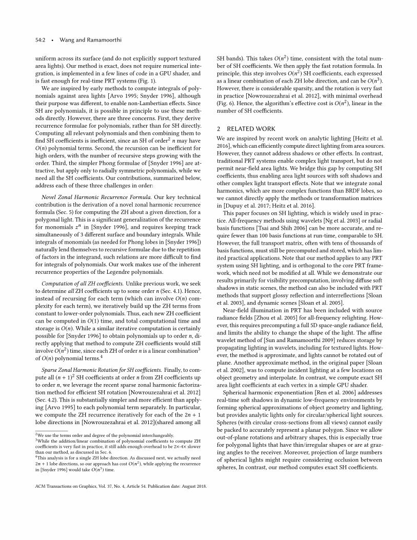
Fig. 1. Images rendered in a PRT system with multiple polygonal arealights, with analytic SH lighting coefficients computed in real-time with ourmethod. This scene contains 388K triangles and is rendered at 28.4 framesper second on an NVIDIA GeForce GTX 1080 Ti GPU.

The core PRT framework precomputes a transfer function for

each vertex on object geometry, taking into account visibility and

BRDF effects. This transfer function is then converted (projected)

into spherical harmonics and stored on the object, possibly with

compression [Sloan et al. 2003]. For soft shadows on a Lambertian

surface, this would simply be an SH representation of the visibility

in each direction. At run-time, these SH coefficients are combined

with the lighting (a simple dot product of SH coefficients of lighting

and transfer for visibility). In this paper, we do not modify the pre-

computation or core PRT framework at all, but address computation

of the SH lighting coefficients. Most PRT methods assume distant,

low-frequency environment map lighting. In this case, the incident

lighting is the same everywhere in the scene, and SH lighting co-

efficients can easily be computed once per frame using standard

numerical integration, and re-used for each vertex on the object.

On the other hand, there is currently limited support for near-field

illumination from area light sources. Indeed, near-field effects imply

that the angular distribution of incident radiance is now different at

each vertex (location in space), and numerical integration to com-

pute SH lighting coefficients separately for each vertex or pixel is

too expensive. In this paper, we address this challenge by develop-

ing an efficient closed-form computation for spherical harmonic

coefficients of general orders, for an arbitrary polygonal area light.

As in most previous work, we assume the light source emission is

ACM Transactions on Graphics, Vol. 37, No. 4, Article 54. Publication date: August 2018.

54:2 • Wang and Ramamoorthi

uniform across its surface (and do not explicitly support textured

area lights). Our method is exact, does not require numerical inte-

gration, is implemented in a few lines of code in a GPU shader, and

is fast enough for real-time PRT systems (Fig. 1).

We are inspired by early methods to compute integrals of poly-

nomials against area lights [Arvo 1995; Snyder 1996], although

their purpose was different, to enable non-Lambertian effects. Since

SH are polynomials, it is possible in principle to use these meth-

ods directly. However, there are three concerns. First, they derive

recurrence formulae for polynomials, rather than for SH directly.

Computing all relevant polynomials and then combining them to

find SH coefficients is inefficient, since an SH of order2 n may have

O(n) polynomial terms. Second, the recursion can be inefficient for

high orders, with the number of recursive steps growing with the

order. Third, the simpler Phong formulae of [Snyder 1996] are at-

tractive, but apply only to radially symmetric polynomials, while we

need all the SH coefficients. Our contributions, summarized below,

address each of these three challenges in order:

Novel Zonal Harmonic Recurrence Formula. Our key technical

contribution is the derivation of a novel zonal harmonic recurrence

formula (Sec. 5) for computing the ZH about a given direction, for a

polygonal light. This is a significant generalization of the recurrence

for monomials zn in [Snyder 1996], and requires keeping track

simultaneously of 3 different surface and boundary integrals. While

integrals of monomials (as needed for Phong lobes in [Snyder 1996])

naturally lend themselves to recursive formulae due to the repetition

of factors in the integrand, such relations are more difficult to find

for integrals of polynomials. Our work makes use of the inherent

recurrence properties of the Legendre polynomials.

Computation of all ZH coefficients. Unlike previous work, we seekto determine all ZH coefficients up to some order n (Sec. 4.1). Hence,

instead of recursing for each term (which can involve O(n) com-

plexity for each term), we iteratively build up the ZH terms from

constant to lower-order polynomials. Thus, each new ZH coefficient

can be computed in O(1) time, and total computational time and

storage is O(n). While a similar iterative computation is certainly

possible for [Snyder 1996] to obtain polynomials up to order n, di-rectly applying that method to compute ZH coefficients would still

involveO(n2) time, since each ZH of ordern is a linear combination3

of O(n) polynomial terms.4

Sparse Zonal Harmonic Rotation for SH coefficients. Finally, to com-

pute all (n + 1)2 SH coefficients at order n from ZH coefficients up

to order n, we leverage the recent sparse zonal harmonic factoriza-

tion method for efficient SH rotation [Nowrouzezahrai et al. 2012]

(Sec. 4.2). This is substantially simpler and more efficient than apply-

ing [Arvo 1995] to each polynomial term separately. In particular,

we compute the ZH recurrence iteratively for each of the 2n + 1

lobe directions in [Nowrouzezahrai et al. 2012](shared among all

2We use the terms order and degree of the polynomial interchangeably.

3While the addition/linear combination of polynomial coefficients to compute ZH

coefficients is very fast in practice, it still adds enough overhead to be 2×-4× slower

than our method, as discussed in Sec. 6.

4This analysis is for a single ZH lobe direction. As discussed next, we actually need

2n + 1 lobe directions, so our approach has cost O (n2), while applying the recurrence

in [Snyder 1996] would take O (n3) time.

SH bands). This takes O(n2) time, consistent with the total num-

ber of SH coefficients. We then apply the fast rotation formula. In

principle, this step involves O(n2) SH coefficients, each expressed

as a linear combination of each ZH lobe direction, and can beO(n3).However, there is considerable sparsity, and the rotation is very fast

in practice [Nowrouzezahrai et al. 2012], with minimal overhead

(Fig. 6). Hence, the algorithm’s effective cost is O(n2), linear in the

number of SH coefficients.

2 RELATED WORKWe are inspired by recent work on analytic lighting [Heitz et al.

2016], which can efficiently compute direct lighting from area sources.

However, they cannot address shadows or other effects. In contrast,

traditional PRT systems enable complex light transport, but do not

permit near-field area lights. We bridge this gap by computing SH

coefficients, thus enabling area light sources with soft shadows and

other complex light transport effects. Note that we integrate zonal

harmonics, which are more complex functions than BRDF lobes, so

we cannot directly apply the methods or transformation matrices

in [Dupuy et al. 2017; Heitz et al. 2016].

This paper focuses on SH lighting, which is widely used in prac-

tice. All-frequency methods using wavelets [Ng et al. 2003] or radial

basis functions [Tsai and Shih 2006] can be more accurate, and re-

quire fewer than 100 basis functions at run-time, comparable to SH.

However, the full transport matrix, often with tens of thousands of

basis functions, must still be precomputed and stored, which has lim-

ited practical applications. Note that our method applies to any PRT

system using SH lighting, and is orthogonal to the core PRT frame-

work, which need not be modified at all. While we demonstrate our

results primarily for visibility precomputation, involving diffuse soft

shadows in static scenes, the method can also be included with PRT

methods that support glossy reflection and interreflections [Sloan

et al. 2003], and dynamic scenes [Sloan et al. 2005].

Near-field illumination in PRT has been included with source

radiance fields [Zhou et al. 2005] for all-frequency relighting. How-

ever, this requires precomputing a full 5D space-angle radiance field,

and limits the ability to change the shape of the light. The affine

wavelet method of [Sun and Ramamoorthi 2009] reduces storage by

propagating lighting in wavelets, including for textured lights. How-

ever, the method is approximate, and lights cannot be rotated out of

plane. Another approximate method, in the original paper [Sloan

et al. 2002], was to compute incident lighting at a few locations on

object geometry and interpolate. In contrast, we compute exact SH

area light coefficients at each vertex in a simple GPU shader.

Spherical harmonic exponentiation [Ren et al. 2006] addresses

real-time soft shadows in dynamic low-frequency environments by

forming spherical approximations of object geometry and lighting,

but provides analytic lights only for circular/spherical light sources.

Spheres (with circular cross-sections from all views) cannot easily

be packed to accurately represent a planar polygon. Since we allow

out-of-plane rotations and arbitrary shapes, this is especially true

for polygonal lights that have thin/irregular shapes or are at graz-

ing angles to the receiver. Moreover, projection of large numbers

of spherical lights might require considering occlusion between

spheres, In contrast, our method computes exact SH coefficients.

ACM Transactions on Graphics, Vol. 37, No. 4, Article 54. Publication date: August 2018.

Analytic Spherical Harmonic Coefficients for Polygonal Area Lights • 54:3

Table 1. Table of notation for key symbols.

Ylm The SH basis function of degree l , indexmLlm The SH coefficient for the polygonal light

Pl Legendre polynomial of degree lQ The polygonal light (projected to unit sphere)

ωe Projection of vertex e onto unit sphere

γe Angle between polygonal vertices e and e + 1ω Central axis of zonal harmonic lobe

αml,d Weight of d-th ZH lobe used to reconstruct YlmSl The surface integral of the l-th Legendre polynomial∫

Q Pl (ω ·ωi )dωi

Bl,e The edge integral

∫ γe0

Pl (ze )dγ

Cl,e The intermediate edge integral

∫ γe0

zePl (ze )dγ

Dl,e The intermediate edge integral

∫ γe0

P ′l (ze )dγ

As noted earlier, we build on [Arvo 1995; Snyder 1996]. Like them,

we assume uniform polygonal planar area lights.We do not explicitly

handle texture, but in some cases, can do so by breaking the light

into smaller polygons, each of which has a uniform color (Fig. 10).

In future, it may be possible to leverage [Chen and Arvo 2001] for

linearly-varying luminaires and angularly-varying lighting.

Finally, the concurrent work of [Belcour et al. 2018] computes

a single integral of a particular SH expansion against a polygon.

We differ conceptually in simultaneously computing integrals of all

SH coefficients, enabling PRT with any SH expansion. In practice,

the methods are quite similar, and [Belcour et al. 2018] also uses a

zonal harmonic decomposition and combines closed-formmonomial

integrals [Arvo 1995; Snyder 1996]. We differ in deriving a novel

zonal harmonic recurrence, rather than combining monomials, and

we demonstrate real-time performance. Although our paper focuses

on PRT, the various other applications mentioned by [Belcour et al.

2018] apply to our method as well, such as basis function projection,

hierarchical sample warping, and use in offline rendering.

3 BACKGROUNDIn this section, we introduce some relevant background. We first

introduce the basic reflection and PRT equations for direct lighting,

focusing on Lambertian surfaces with soft shadowing for simplic-

ity (more complex light transport can also be included, since our

method is orthogonal to the core PRT framework). We then briefly

introduce the spherical harmonics and integration against an area

light, ending with some key SH and Legendre polynomial formulas.

Table 1 summarizes notation for key symbols used in the paper.

3.1 Precomputed Radiance TransferThe reflection equation for direct lighting can be written,

Lr (x ,ωr ) =

∫ΩLi (x ,ωi )V (x ,ωi )ρ(ωi ,ωr ,n)max(ωi · n, 0)dωi ,

(1)

where x is the spatial coordinate of the current vertex or pixel,

(ωi ,ωr ) are the global incoming and outgoing directions, and n is

the surface normal. Lr is the reflected radiance or image intensity,

whileLi is the incident radiance.5V is the visibility and ρ is the BRDF(which includes the normal as an argument, since it is expressed in

terms of incoming and outgoing directions in global coordinates).

For simplicity of notation, we combine the visibility and BRDF

terms into a transport function T (x ,ωi ), which is precomputed for

each spatial location x and incident angleωi . We have dropped the

dependence onωr for simplicity, but that can also be expressed in

spherical harmonics [Sloan et al. 2002], and glossy reflections are

demonstrated in Fig. 10. We may now write,

Lr (x) =

∫ΩLi (x ,ωi )T (x ,ωi )dωi . (2)

To proceed further, we project the lighting and transport func-

tion into spherical harmonics Ylm (ωi ) with l ≥ 0 the order, and

−l ≤ m ≤ l . We will discuss the spherical harmonic basis function

forms [MacRobert 1948] briefly at the end of this section. We use

spherical harmonics up to degree n with (n + 1)2 terms; we demon-

strate results for fairly high order spherical harmonics with n = 8 or

n = 14, and our results are general for even higher orders if needed,

Li (x ,ωi ) =

n∑l=0

l∑m=−l

Llm (x)Ylm (ωi )

T (x ,ωi ) =

n∑l=0

l∑m=−l

Tlm (x)Ylm (ωi ). (3)

Given these coefficients, by orthonormality of the basis functions,

Lr (x) =n∑l=0

l∑m=−l

Llm (x)Tlm (x) = L(x) ·T (x), (4)

where L andT are vector representations of Llm and Tlm , and the

integral can be reduced to a simple dot product.

3.2 Area Light IntegrationNote that Tlm is precomputed, based on numerical integration in

the standard way for PRT methods. The major contribution of thispaper is to derive a closed form formula for Llm from polygonal arealights. In particular, we seek a solution to

Llm =

∫Qx

Ylm (ωi )dωi , (5)

where the integral is over the projection of the polygon Q onto the

unit sphere. Note that we work with the real (not complex) spherical

harmonics. In addition, we have dropped the spatial coordinate xin Llm , since it is easy to translate the polygon so x is at the origin;

we denote this using Qx , but will drop the subscript in Sec. 4, to

simplify notation.

We will first seek to determine the zonal harmonic coefficients

(m = 0) corresponding to a particular central directionω,

Ll (ω) =

∫Qx

Yl0(ω ·ωi )dωi . (6)

5We use superscripts for Lr and Li to avoid confusion with subscripts such as Llmfor spherical harmonic coefficients.

ACM Transactions on Graphics, Vol. 37, No. 4, Article 54. Publication date: August 2018.

54:4 • Wang and Ramamoorthi

3.3 Spherical Harmonic FormulasFinally, we briefly discuss the mathematical forms we use for the

spherical harmonics and zonal harmonics in this paper, along with

relevant identities. Consider the geographic angular parameteri-

zation of the sphere (θ ,ϕ) with Cartesian components, (x ,y, z) =(sinθ cosϕ, sinθ sinϕ, cosθ ). The real spherical harmonics are,

Ylm (θ ,ϕ) =

√(2l + 1)

4π

(l− |m |)!

(l+ |m |)!P|m |

l (cosθ ) f (|m |ϕ) , (7)

where P lm are the associated Legendre polynomials and the trigono-

metric function f (|m |ϕ) is set to 1whenm = 0, given by

√2 cos(mϕ)

whenm > 0 and

√2 sin(|m |ϕ) whenm < 0. In particular, the zonal

harmonics (ZH) form = 0 are given by,

Yl0(cosθ ) =

√2l + 1

4πPl (cosθ ), (8)

where we parameterize by cosθ = z, and Pl (z) are simply the Le-

gendre polynomials of degree l . For example P0(z) = 1, P1(z) = zand P2(z) =

1

2(3z2 −1). Note that the ZH are radially symmetric and

independent of ϕ, depending only on z in a Cartesian coordinate

system. To consider ZH lobes (as a function of incident direction

ωi = (θ ,ϕ)) about an arbitrary axisω, we can simply use a dot prod-

uct with that axis, defining the ZH as Yl0(ω ·ωi ) as in equation 6.

A key result relating SH and ZH enables sparse ZH factorization

of SH, and allows for fast rotation of ZH into SH. [Nowrouzezahrai

et al. 2012] show6that for anym and any order l (for consistency

with equation 6 we useωi = (θ ,ϕ)),

Ylm (ωi ) =∑d

αml,dYl0(ωl,d ·ωi ). (9)

That is, an SH of degree l can always be written as a sum of rotated

ZH basis functions. While d can in principle range from −l to +l ,involving 2l + 1 lobes, the actual number of lobes needed is usually

much smaller. Moreover, the same lobes are used across a band l ,and in fact one can optimize to share directionsωl,d across bands.

As such, there are only 2n + 1 unique lobe directions ω across all

bands, and the weights αl,d are very sparse. [Nowrouzezahrai et al.

2012] have already precomputed the lobe directions and weights.

Finally, we will make use of some well-known relations for Le-

gendre polynomials in the subsequent derivations in Sec. 5 (below,

P ′l (z) stands for the derivativeddz Pl (z)),

z2 − 1

lP ′l (z) = zPl (z) − Pl−1(z) (10)

lPl (z) = (2l − 1)zPl−1(z) − (l − 1)Pl−2(z) (11)

(2l + 1)Pl (z) = P ′l+1(z) − P ′l−1(z) (12)

4 ALGORITHMIn this section, we introduce our algorithm for computing the ana-

lytic SH coefficients for a polygonal area light source, i.e., determin-

ing Llm in equation 5. The key technical contribution is the novel

zonal harmonic recurrence, which is derived later in Sec. 5. While

the mathematics and derivation is somewhat involved, the actual

implementation is simple, as discussed at the end of Sec. 4.1 and

6Versions of equation 9 appear earlier in other fields, going back at least to [Stern 1965].

(a)

(b)

(d)

(c)

Fig. 2. Illustration of the integrals we keep track of (surface, boundary). In(a), we show the projection of the polygon to the unit sphere with supportQ . In (b) we show the corresponding surface integral Sl , while (c) showsthe boundary integral Bl . Note that Bl can be broken into edges or arcsBl,e as shown in (d) using a very simple parameterization. We also keeptrack of intermediate boundary integral Dl,e , and compute Cl,e on the fly.

shown in the pseudocode in Algorithm 1. In practice, the algorithm

is implemented in a simple GPU vertex shader, and the source code

is publicly available at http://viscomp.ucsd.edu/projects/ash.

4.1 Iterative Computation of Zonal Harmonic CoefficientsWe first develop an iterative algorithm to compute the zonal har-

monics coefficients, Ll (equation 6). Doing so requires iteratively

updating the surface integral, as well as two boundary integrals (a

third boundary integral is computed on the fly). Figure 2 shows the

quantities we keep track of. We start by defining the integrals we

need and relevant notation and quantities, then discuss the base

cases, and finally state the recurrence relation. Then, we summarize

the iterative algorithm with reference to the pseudocode in Alg. 1.

Surface and Boundary Integrals. We assume the polygon has been

translated by −x , so the spatial location of the vertex is at the origin,

as shown in Fig. 2(a), and omit explicit dependence on x in what

follows. We are now primarily interested in the surface integral

(Fig. 2(b)),

Sl =

∫QPl (ω ·ωi )dωi Ll =

√2l + 1

4πSl . (13)

Sl simply integrates the projection of the area light on the unit

sphere against Legendre polynomials Pl of the dot productω ·ωi .

We can multiply in the (precomputed) normalization constant at

the end to compute final ZH coefficient Ll . Note that Sl is computed

separately for each lobe direction ωl,d (there may be 2n + 1 suchdirections). For simplicity of notation, we just useω, as in equation 6,

and omit the explicit dependence of Sl onω.

ACM Transactions on Graphics, Vol. 37, No. 4, Article 54. Publication date: August 2018.

Analytic Spherical Harmonic Coefficients for Polygonal Area Lights • 54:5

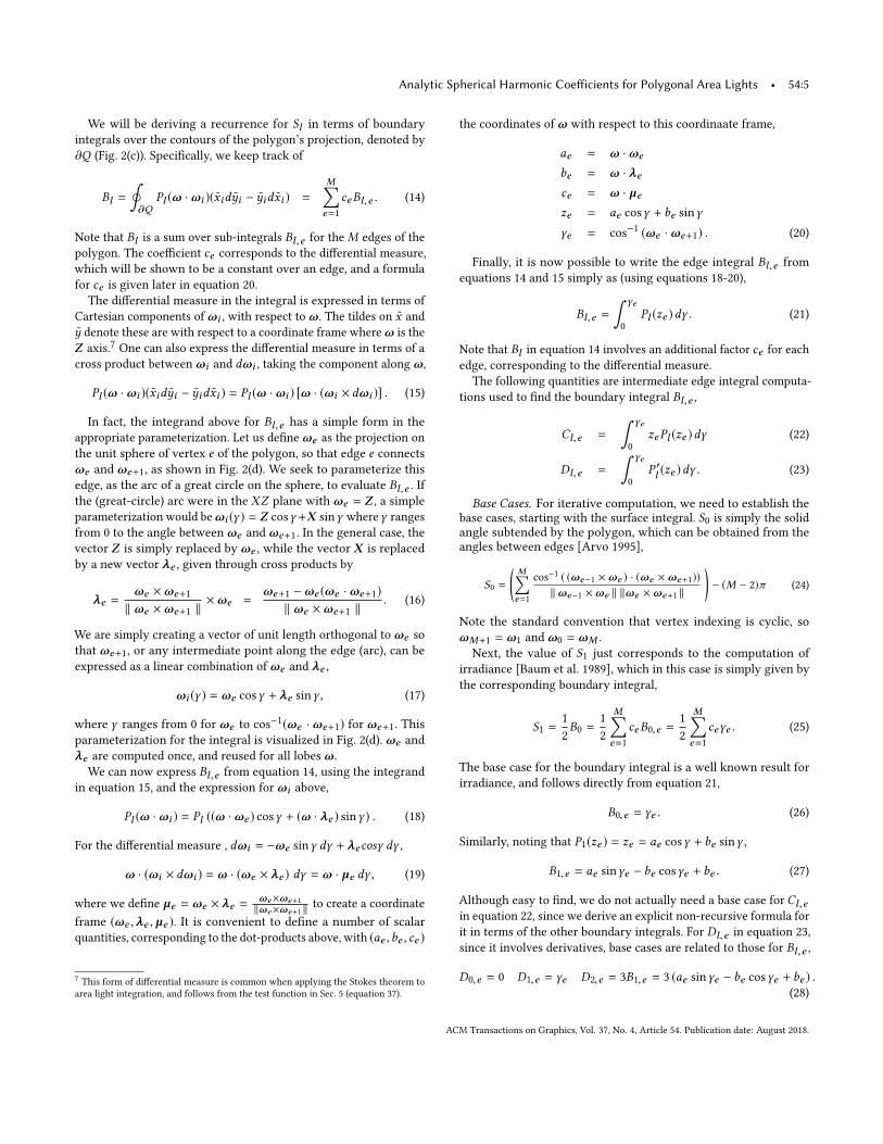
We will be deriving a recurrence for Sl in terms of boundary

integrals over the contours of the polygon’s projection, denoted by

∂Q (Fig. 2(c)). Specifically, we keep track of

Bl =

∮∂Q

Pl (ω ·ωi )(xidyi − yidxi ) =M∑e=1

ceBl,e . (14)

Note that Bl is a sum over sub-integrals Bl,e for theM edges of the

polygon. The coefficient ce corresponds to the differential measure,

which will be shown to be a constant over an edge, and a formula

for ce is given later in equation 20.

The differential measure in the integral is expressed in terms of

Cartesian components ofωi , with respect toω. The tildes on x and

y denote these are with respect to a coordinate frame whereω is the

Z axis.7One can also express the differential measure in terms of a

cross product betweenωi and dωi , taking the component alongω,

Pl (ω ·ωi )(xidyi − yidxi ) = Pl (ω ·ωi ) [ω · (ωi × dωi )] . (15)

In fact, the integrand above for Bl,e has a simple form in the

appropriate parameterization. Let us defineωe as the projection on

the unit sphere of vertex e of the polygon, so that edge e connectsωe and ωe+1, as shown in Fig. 2(d). We seek to parameterize this

edge, as the arc of a great circle on the sphere, to evaluate Bl,e . Ifthe (great-circle) arc were in the XZ plane with ωe = Z , a simple

parameterization would beωi (γ ) = Z cosγ +X sinγ whereγ ranges

from 0 to the angle betweenωe andωe+1. In the general case, the

vector Z is simply replaced by ωe , while the vector X is replaced

by a new vector λe , given through cross products by

λe =ωe ×ωe+1

∥ ωe ×ωe+1 ∥×ωe =

ωe+1 −ωe (ωe ·ωe+1)

∥ ωe ×ωe+1 ∥. (16)

We are simply creating a vector of unit length orthogonal to ωe so

that ωe+1, or any intermediate point along the edge (arc), can be

expressed as a linear combination ofωe and λe ,

ωi (γ ) = ωe cosγ + λe sinγ , (17)

where γ ranges from 0 for ωe to cos−1(ωe · ωe+1) for ωe+1. This

parameterization for the integral is visualized in Fig. 2(d).ωe and

λe are computed once, and reused for all lobesω.

We can now express Bl,e from equation 14, using the integrand

in equation 15, and the expression forωi above,

Pl (ω ·ωi ) = Pl ((ω ·ωe ) cosγ + (ω · λe ) sinγ ) . (18)

For the differential measure , dωi = −ωe sinγ dγ + λecosγ dγ ,

ω · (ωi × dωi ) = ω · (ωe × λe ) dγ = ω · µe dγ , (19)

where we define µe = ωe × λe =ωe×ωe+1∥ωe×ωe+1 ∥

to create a coordinate

frame (ωe ,λe , µe ). It is convenient to define a number of scalar

quantities, corresponding to the dot-products above, with (ae ,be , ce )

7This form of differential measure is common when applying the Stokes theorem to

area light integration, and follows from the test function in Sec. 5 (equation 37).

the coordinates ofω with respect to this coordinaate frame,

ae = ω ·ωe

be = ω · λe

ce = ω · µe

ze = ae cosγ + be sinγ

γe = cos−1 (ωe ·ωe+1) . (20)

Finally, it is now possible to write the edge integral Bl,e from

equations 14 and 15 simply as (using equations 18-20),

Bl,e =

∫ γe

0

Pl (ze )dγ . (21)

Note that Bl in equation 14 involves an additional factor ce for each

edge, corresponding to the differential measure.

The following quantities are intermediate edge integral computa-

tions used to find the boundary integral Bl,e ,

Cl,e =

∫ γe

0

zePl (ze )dγ (22)

Dl,e =

∫ γe

0

P ′l (ze )dγ . (23)

Base Cases. For iterative computation, we need to establish the

base cases, starting with the surface integral. S0 is simply the solid

angle subtended by the polygon, which can be obtained from the

angles between edges [Arvo 1995],

S0 =

(M∑e=1

cos−1 ( (ωe−1 ×ωe ) · (ωe ×ωe+1))

∥ωe−1 ×ωe ∥ ∥ωe ×ωe+1 ∥

)− (M − 2)π (24)

Note the standard convention that vertex indexing is cyclic, so

ωM+1 = ω1 andω0 = ωM .

Next, the value of S1 just corresponds to the computation of

irradiance [Baum et al. 1989], which in this case is simply given by

the corresponding boundary integral,

S1 =1

2

B0 =1

2

M∑e=1

ceB0,e =1

2

M∑e=1

ceγe . (25)

The base case for the boundary integral is a well known result for

irradiance, and follows directly from equation 21,

B0,e = γe . (26)

Similarly, noting that P1(ze ) = ze = ae cosγ + be sinγ ,

B1,e = ae sinγe − be cosγe + be . (27)

Although easy to find, we do not actually need a base case for Cl,ein equation 22, since we derive an explicit non-recursive formula for

it in terms of the other boundary integrals. For Dl,e in equation 23,

since it involves derivatives, base cases are related to those for Bl,e ,

D0,e = 0 D1,e = γe D2,e = 3B1,e = 3 (ae sinγe − be cosγe + be ) .(28)

ACM Transactions on Graphics, Vol. 37, No. 4, Article 54. Publication date: August 2018.

54:6 • Wang and Ramamoorthi

Recurrence Relation. In Sec. 5, we derive the recurrence relations

for surface and boundary integrals. Combined with the base cases

above, these enable us to start with S0, S1, B0,B1 and D0,D1,D2,

iterating to build up higher values of Sl and Bl until we reach Sn .Specifically, we derive that

Sl =2l − 1

l(l + 1)Bl−1 +

(l − 2)(l − 1)

l(l + 1)Sl−2. (29)

This is a direct O(1) iterative expression for Sl assuming Bl−1 andSl−2 have already been computed. However, to compute Sl+1, wewill also need an iterative formula for the boundary integral, Bl ,which is derived for each edge as,

Bl,e =2l − 1

lCl−1,e −

l − 1

lBl−2,e . (30)

An explicit formula for the boundary integral Cl−1,e is derived in

the appendix,

Cl−1,e =1

l((ae sinγe − be cosγe ) Pl−1(ae cosγe + be sinγe )

+bePl−1(ae ) + (a2

e + b2

e − 1)Dl−1,e + (l − 1)Bl−2,e )(31)

Finally, there is a simple recurrence for D,

Dl,e = (2l − 1)Bl−1,e + Dl−2,e . (32)

After we compute the base cases, we iterate 2 ≤ l ≤ n, storingthe values of Sl for increasing orders, while also updating Bl andDl per the recurrence formulas above. Note that each iteration

for increasing l is constant time, and the whole time and storage

complexity is O(n). Further note that Cl−1,e is computed explicitly

on the fly and does not require storage. Moreover, we do not need to

store all values of the boundary integrals B and D. Indeed, we needonly keep the three intermediate values of Dl−2,e ,Dl−1,e ,Dl,e , and

can discard older values, with a similar strategy employed for B.

Iterative Computation. The pseudocode in Algorithm 1 details

the iterative computation, given spatial location x and a polygon

with verticesve ofM sides. The lobe weights αml,d for ZH rotation,

along with lobe directions ωl,d are also inputs. We compute SH

coefficients up to order n.First (Line 2), we translate the polygon vertices by −x and project

onto the unit sphere, obtaining the verticesωe on the sphere. The

quantities λe , µe = ωe × λe and γe are also pre-calculated at this

stage for each edge (Lines 3-7). Finally, the solid angle of the polygon

S0 is computed (Line 8). We now enter the iterative computation,

which is repeated for each lobe directionω (Line 9). We calculate

ae , be and ce as per equation 20 (Line 12), and the base cases for

B0,e ,B1,e (Lines 14-15) and D1,e ,D2,e (Line 16). For the base case

S1, we must sum over all edges (Lines 10,13).

Then, we iterate 2 ≤ l ≤ n (Line 18), and update the boundary

integrals for each edge (Lines 20-25). Specifically we computeCl−1,e(Line 21), and apply the recurrence formulae for Bl,e (Line 22) and

Dl,e (Line 24). The boundary integral Bl is updated by summing

over edge integrals Bl,e (Lines 19, 23). For clarity, we do not include

a number of practical storage optimizations. Only a single variable

C needs to be used for Cl−1,e since it is computed explicitly. As

discussed earlier, we only need to maintain the three most recent

values forB andD. Finally, we update the surface integral Sl (Line 26)

Algorithm 1 Pseudocode of algorithm for SH coefficients.

1: function ComputeCoefficients(x ,v[], M, n, α[],ω[])

2: forall e:ve = ve − x ;ωe =ve∥ve ∥

▷ Project to Sphere

3: for e = 1 toM do ▷ Pre-Calculate per edge

4: λe =ωe×ωe+1∥ωe×ωe+1 ∥

×ωe ▷ Eq. 16

5: µe = ωe × λe ▷ Frame (ωe ,λe , µe )6: γe = cos

−1 (ωe ·ωe+1) ▷ Angle of edge e Eq. 207: end for8: S0 = SolidAngle(ωe [],M) ▷ Eq. 24

9: for allω inω[] do ▷ Up to 2n+1 for all bands

10: S1 = 0 ▷ Initialize S111: for e = 1 toM do ▷ Base Cases

12: ae = ω ·ωe ; be = ω · λe ; ce = ω · µe ▷ Eq. 20

13: S1 = S1 +1

2ceγe ▷ Eq. 25

14: B0,e = γe ▷ Eq. 26

15: B1,e = ae sinγe − be cosγe + be . ▷ Eq. 27

16: D0,e = 0;D1,e = γe ; D2,e = 3B1,e ▷ Eq. 28

17: end for18: for l = 2 to n do ▷ Each degree 2 ≤ l ≤ n19: Bl = 0 ▷ Initialize Bl20: for e = 1 toM do ▷ Edge Integrals

21: Cl−1,e =C(l ,ae ,be ,Bl−2,e ,Dl−1,e ) ▷ Eq. 31

22: Bl,e =2l−1l Cl−1,e − (l − 1)Bl−2,e ▷ Eq. 30

23: Bl = Bl + ceBl,e ▷ Eq. 14

24: Dl,e = (2l − 1)Bl−1,e + Dl−2,e ▷ Eq. 32

25: end for26: Sl =

2l−1l (l+1)Bl−1 +

(l−2)(l−1)l (l+1) Sl−2 ▷ Eq. 29

27: Ll (ω) =

√2l+14π Sl ▷ Eq. 13

28: end for29: end for30: for each SH basis function (l ,m) do ▷ ZH rotation

31: Llm = 0 ▷ Initialize Llm32: for each d ∈ d(l) do ▷ Sparse set of lobesωl,d33: Llm = Llm + α

ml,dLl (ωl,d ) ▷ Eq. 33

34: end for35: end for36: end function

and include the normalization factor to compute the zonal harmonic

coefficients Ll (ω) for each lobe (Line 27).

The last stage is to use the sparse zonal harmonic rotation formula

to get all spherical harmonic coefficients Llm from ZH coefficients

Ll (ω), as discussed in Sec. 4.2 (Lines 30-35).

Discussion. We briefly compare our recurrence with that derived

in [Snyder 1996] for Phong lighting. Ours is a recurrence directly onLegendre polynomials rather than monomials in [Snyder 1996]. Thus,

we directly have the ZH coefficients. In contrast, if we had used

the monomial recurrence from [Snyder 1996], we would have had

to separately compute and sum O(n) monomial integrals for each

ZH coefficient for each lobe, with a total complexity O(n3). Indeed,our direct Legendre polynomial recurrence is the key contribution

of the paper. Note that the derivation and recursive formula is

more complicated since we are dealing with polynomial rather than

ACM Transactions on Graphics, Vol. 37, No. 4, Article 54. Publication date: August 2018.

Analytic Spherical Harmonic Coefficients for Polygonal Area Lights • 54:7

* *

* 1 * 2

+

+

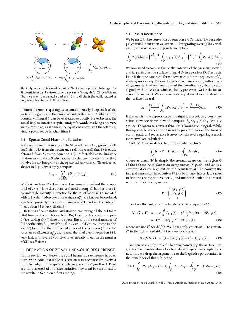
Fig. 3. Sparse zonal harmonic rotation. The SH and equivalently integral forSH coefficients can be viewed as a sparse sum of integrals for ZH coefficients.Thus, we may sum a small number of ZH coefficients (here, illustrated asonly two lobes) for each SH coefficient.

monomial terms, requiring us to simultaneously keep track of the

surface integral S and the boundary integrals B and D, while a thirdboundary integral C can be evaluated explicitly. Nevertheless, the

actual implementation is quite straightforward, involving only very

simple formulae, as shown in the equations above, and the relatively

simple pseudocode in Algorithm 1.

4.2 Sparse Zonal Harmonic RotationWe now proceed to compute all the SH coefficients Llm given the ZH

coefficients Ll from the recurrence relation (recall that Ll is easilyobtained from Sl using equation 13). In fact, the same linearity

relation in equation 9 also applies to the coefficients, since they

involve linear integrals of the spherical harmonics. Therefore, as

shown in Fig. 3, we simply compute,

Llm =∑

d ∈d (l )

αml,dLl(ωl,d

). (33)

While d can take 2l + 1 values in the general case (and there are a

total of 2n + 1 lobe directionsω shared among all bands), there is

considerable sparsity in practice for the set of lobes d(l) associatedwith SH order l . Moreover, the weights αml,d are known beforehand,

as a basic property of spherical harmonics. Therefore, the rotation

in equation 33 is very efficient.

In terms of computation and storage, computing all the ZH takes

O(n) time, and is run for each of O(n) lobe directionsω to compute

Ll (ω), taking O(n2) time and space, linear in the total number of

SH coefficients Llm , which is also O(n2). (Of course, there is alsoa O(M) factor for the number of edges of the polygon.) Since the

rotation coefficients αml,d are sparse, the final step in equation 33 is

very fast, with overall complexity essentially linear in the number

of SH coefficients.

5 DERIVATION OF ZONAL HARMONIC RECURRENCEIn this section, we derive the zonal harmonic recurrence in equa-

tions 29-32. Note that while this section is mathematically involved,

the actual algorithm is quite simple, as shown in Algorithm 1. Read-

ers more interested in implementation may want to skip ahead to

the results in Sec. 6 on a first reading.

5.1 Main RecurrenceWe begin with the derivation of equation 29. Consider the Legendre

polynomial identity in equation 11. Integrating over Q (i.e., with

each term now as an integrand), we obtain∫QPl (z)dωi =

(2l − 1

l

∫QzPl−1(z)dωi

)−

(l − 1

l

∫QPl−2(z)dωi

).

(34)

We now need to convert this to the notation of the previous section,

and in particular the surface integral Sl in equation 13. The main

issue is that the canonical form above uses z for the argument of Pl ,while Sl usesω ·ωi . For our derivation, we can assume, without loss

of generality, that we have rotated the coordinate system so ω is

aligned with the Z axis, while explicitly preservingω for the actual

algorithm in Sec. 4. We can now view equation 34 as a relation for

the surface integral,

Sl =

(2l − 1

l

∫QzPl−1(z)dωi

)−

(l − 1)

lSl−2. (35)

It is clear that the expression on the right is a previously-computed

value. Now we show how to compute

∫Q zPl−1(z)dωi . We use

Stokes’ Theorem to convert this into a boundary integral. While

this approach has been used in many previous works, the form of

our integrals and recurrence is more complicated, requiring a much

more involved calculation.

Stokes’ theorem states that for a suitable vector V ,∫QN · (∇ ×V )dωi =

∮∂Q

V · dr , (36)

where as usual, N is simply the normal at ωi on the region Qof the sphere, with Cartesian components (x ,y, z)t , and dr is a

differential curve segment on the boundary ∂Q . To convert the

integral expression in equation 35 to a boundary integral, we need

to find the appropriate vector V , and further calculations are still

required. Specifically, we use

V =©­«−yPl−1(z)xPl−1(z)

0

ª®¬ (37)

We take the curl, as in the left-hand side of equation 36,

N · (∇ ×V ) = −x2d

dzPl−1(z) − y2

d

dzPl−1(z) + 2zPl−1(z)

= (z2 − 1)P ′l−1(z) + 2zPl−1(z), (38)

where we use P ′ for dP/dz. We now apply equation 10 to rewrite

P ′ in the right-hand side of the above expression,

N · (∇ ×V ) = (l + 1)zPl−1(z) − (l − 1)Pl−2(z). (39)

We can now apply Stokes’ Theorem, converting the surface inte-

gral for the quantity above to a boundary integral. For simplicity of

notation, we drop the argument z to the Legendre polynomials in

the remainder of this subsection,

(l + 1)

∫QzPl−1dωi − (l − 1)

∫Q

Pl−2dωi =

∮∂Q

Pl−1(xdy − ydx).

(40)

ACM Transactions on Graphics, Vol. 37, No. 4, Article 54. Publication date: August 2018.

54:8 • Wang and Ramamoorthi

We can now to evaluate the surface integral

∫Q zPl−1dωi in equa-

tion 35. Including the normalization2l−1l in equation 35 and re-

arranging terms in equation 40,

2l − 1

l

∫QzPl−1dωi = (41)

2l − 1

l(l + 1)

∮∂Q

Pl−1(xdy − ydx) +(2l − 1)(l − 1)

l(l + 1)

∫QPl−2dωi .

Substituting this result back into equation 35 gives

Sl =2l − 1

l(l + 1)Bl−1 +

(2l − 1)(l − 1)

l(l + 1)Sl−2 −

(l − 1)

lSl−2

Sl =2l − 1

l(l + 1)Bl−1 +

(l − 2)(l − 1)

l(l + 1)Sl−2, (42)

which is exactly the main recurrence in equation 29.

5.2 Boundary IntegralsNow we derive a recurrence for the boundary integral Bl , whichis simply a sum of edge integrals Bl,e , as in equation 21. We are

interested in Bl,e =∫ γe0

Pl (ze )dγ , where as usual we have that

ze = ae cosγ + be sinγ . We first rewrite Bl,e using equation 11,∫ γe

0

Pl (ze )dγ =21 − 1

l

∫ γe

0

zePl−1(ze )dγ −l − 1

l

∫ γe

0

Pl−2(ze )dγ .

(43)

The integrals correspond respectively to Bl,e on the left-hand side,

and Cl−1,e and Bl−2,e on the right-hand side. Considering the nor-

malization factors, this is exactly the recurrence relation for Bl,e in

equation 30. It is clear that the second term on the right has been

previously computed. The first term on the right corresponds to

Cl−1,e =∫zePl−1(ze )dγ . In the appendix, we derive an explicit

formula for Cl,e , using integration by parts, deriving equation 31.

Finally, to compute Dl,e , we can use equation 12, which we

rewrite as (2l − 1)Pl−1(z) = P ′l (z) − P ′l−2(z). Considering the corre-sponding integrals and rearranging,∫ γe

0

P ′l (ze )dγ = (2l−1)

∫ γe

0

Pl−1(ze )dγ+

∫ γe

0

P ′l−2(ze )dγ . (44)

This can be written as Dl,e = (2l − 1)Bl−1,e + Dl−2,e , which gives

the recurrence in equation 32.

6 IMPLEMENTATION AND RESULTSThe algorithm is implemented in a simple GPU vertex shader, which

computes SH coefficients separately at each vertex, following the

pseudocode in Algorithm 1. We store pre-tabulated values of Le-

gendre polynomials in 1D textures, which are interpolated in hard-

ware and fetched within the shader program. This effectively allows

the Legendre polynomial evaluations in equation 31 to be evaluated

in constant time. Once the SH lighting coefficients are computed,

they can directly be used in the PRT system. Moreover, the SH light-

ing coefficients can also be added to those from an environment

map or from other lights to render images with multiple area light

sources and environment lighting (Figs. 1,9).

Analysis of Accuracy. The spherical harmonic formula in Sec. 4 is

exact. To verify the correctness of the formula and its derivation, we

compare with numerical integration with 146k samples per vertex

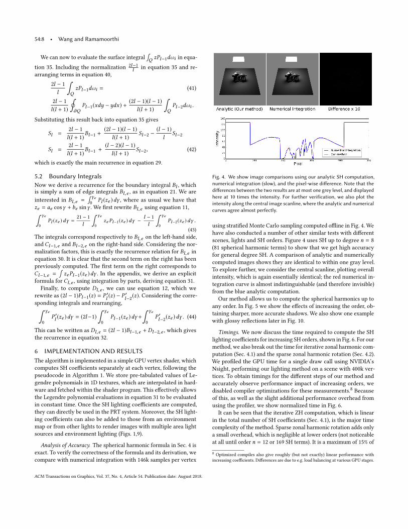
Fig. 4. We show image comparisons using our analytic SH computation,numerical integration (slow), and the pixel-wise difference. Note that thedifferences between the two results are at most one grey level, and displayedhere at 10 times the intensity. For further verification, we also plot theintensity along the central image scanline, where the analytic and numericalcurves agree almost perfectly.

using stratified Monte Carlo sampling computed offline in Fig. 4. We

have also conducted a number of other similar tests with different

scenes, lights and SH orders. Figure 4 uses SH up to degree n = 8

(81 spherical harmonic terms) to show that we get high accuracy

for general degree SH. A comparison of analytic and numerically

computed images shows they are identical to within one gray level.

To explore further, we consider the central scanline, plotting overall

intensity, which is again essentially identical; the red numerical in-

tegration curve is almost indistinguishable (and therefore invisible)

from the blue analytic computation.

Our method allows us to compute the spherical harmonics up to

any order. In Fig. 5 we show the effects of increasing the order, ob-

taining sharper, more accurate shadows. We also show one example

with glossy reflections later in Fig. 10.

Timings. We now discuss the time required to compute the SH

lighting coefficients for increasing SH orders, shown in Fig. 6. For our

method, we also break out the time for iterative zonal harmonic com-

putation (Sec. 4.1) and the sparse zonal harmonic rotation (Sec. 4.2).

We profiled the GPU time for a single draw call using NVIDIA’s

Nsight, performing our lighting method on a scene with 400k ver-

tices. To obtain timings for the different steps of our method and

accurately observe performance impact of increasing orders, we

disabled compiler optimizations for these measurements.8Because

of this, as well as the slight additional performance overhead from

using the profiler, we show normalized time in Fig. 6.

It can be seen that the iterative ZH computation, which is linear

in the total number of SH coefficients (Sec. 4.1), is the major time

complexity of the method. Sparse zonal harmonic rotation adds only

a small overhead, which is negligible at lower orders (not noticeable

at all until order n = 12 or 169 SH terms). It is a maximum of 15% of

8Optimized compiles also give roughly (but not exactly) linear performance with

increasing coefficients. Differences are due to e.g. load balancing at various GPU stages.

ACM Transactions on Graphics, Vol. 37, No. 4, Article 54. Publication date: August 2018.

Analytic Spherical Harmonic Coefficients for Polygonal Area Lights • 54:9

Fig. 5. Area lighting with SH orders 2, 4, 6, and 8. Note increasing accuracyin terms of sharpness of shadows with higher orders.

Fig. 6. Plot of timings for increasing numbers of spherical harmonic coef-ficients. Note that the rotation step is negligible at lower orders, and theoverall method is therefore linear in the number of SH coefficients.

total runtime at order n = 14 (225 SH terms). Thus, in practice, the

time complexity of our method is O(n2) or linear in the number of

SH coefficients, as desired. Finally, Fig. 7 plots normalized runtime

vs. the number of light polygon edges M . As expected the time

complexity is linear in the number of edges (or vertices) of the

polygonal area light.

We now discuss actual wall-clock running times, using anNVIDIA

GeForce GTX 1080 Ti GPU, with compiler optimizations enabled.

For the plant scene in Fig. 5 with 163K triangles and one rectangular

area light, at SH order n = 8, our method runs at 350 frames per

second. We also compared with using the monomial recurrence

in [Snyder 1996] (the direct computation per [Arvo 1995] would be

even slower). To do so, we used our iterative method to compute

the monomials instead of the ZH, followed by combining them to

compute the ZH coefficients, and then using our sparse SH rotation.

Fig. 7. Plot of timings for increasing the number of edges (vertices) in thepolygonal area light, showing the method behaves linearly.

Table 2. Running time for our method in frames per second. We also includea comparison to using the monomial recurrence in [Snyder 1996].

Scene Tris. Lights Speed (Us) Monomial

Plant (Fig. 5) 163k 1 350.0 fps 91.0 fps

Buddha (Fig. 1) 388k 3 28.4 fps 8.2 fps

Dragon (Fig. 9) 1M 1 38.5 fps 15.3 fps

Face (Fig. 8) 98k 1 384.6 fps 150.0 fps

Note that this is not the method of [Snyder 1996], since we only use

their recurrence, and only one part differs from ours (computation

of monomials rather than directly using the ZH recurrence). That

method ran about 4× slower, at 91fps because of the time complexity

in linearly combining monomials to obtain ZH. While the compiler

can optimize the required additions to make them very fast, the extra

O(n) complexity for linear combinations of monomials still adds

significant overhead. Table 2 shows additional runtime comparisons

on a variety of scenes. The complexity depends on polygon count

and the number of lights, achieving 300+fps for models of about

100K triangles and one light (Figs. 5, 8), and still being real-time at

28-39fps for the 1M polygon dragon scene in Fig. 9 as well as the

388K polygon Buddha scene in Fig. 1 with three polygonal lights.

In all cases, our algorithm is 2×–4× faster than using the monomial

recurrence of [Snyder 1996].

Applications. A number of applications and extensions enabled

by our approach can be seen in the accompanying video and are

briefly described here. Our method supports general polygonal area

lights, and enables editing of the light source, rotations, or transla-

tions as shown in Fig. 8. (The scene can also be rotated/translated,

corresponding to an inverse transformation of the lights). Moreover,

multiple area lights can be combined, simply by adding their SH

coefficients (Fig. 1). The time complexity for SH lighting calcula-

tion will grow linearly with the number of lights, but the cost of

lighting-visibility computation in the PRT framework is not affected,

since it need only be done once at the end. We can also include en-

vironment maps (Fig. 9), with their SH coefficients computed in the

conventional way by numerical integration once per frame, and

then simply added to the analytic area light SH coefficients.

ACM Transactions on Graphics, Vol. 37, No. 4, Article 54. Publication date: August 2018.

54:10 • Wang and Ramamoorthi

Fig. 8. Our method supports translation, in/out of plane rotations, andediting of the shape of the light source. Insets show area light positions. Inthis example, we show SH order n = 8.

Finally, while we do not support textured lights (since the deriva-

tion and formulae assume constant emission over the polygon), we

can in some cases break the area light into smaller polygons, each

with a different color. Since we only use low-order spherical har-

monics, detailed textures are not needed. An example is shown in

Fig. 10. This result also uses a glossy ground reflector and Buddha,

leading to appearance that switches from reddish to bluish, in ac-

cordance with the light texture, from one end of the ground plane

to the other. Similarly, the Buddha has bluish as well as yellow-

ish highlights (combining red and green parts of the light). Glossy

reflection is computed using spherical harmonic triple products

(Clebsch-Gordan coefficients) to multiply the precomputed visibility

and area lighting computed with our method at each vertex, before

convolving with a Phong BRDF [Sloan et al. 2002].

7 CONCLUSIONS AND FUTURE WORKSpherical Harmonic lighting is a popular technique today for real-

time applications based on the precomputed radiance transfermethod.

We enable the use of near-field polygonal area lights, almost as eas-

ily as distant environment map lighting, by deriving analytic results

for integrating spherical harmonics against planar polygons. The

key technical contribution is a novel recurrence directly for zonal

harmonic coefficients, which enables all coefficients up to a given

degree to be computed iteratively in linear time, followed by fast

spherical harmonic rotation. The algorithm is implemented in a

simple GPU shader for area lighting within any spherical harmonic

lightingmethod. In the future, wewould like to generalize the results

to non-uniform or directional emission.

So far, we have not exploited the smoothness of area lighting.

This can be done in at least two ways. First, the SH coefficients are

Fig. 9. Our method can support traditional relighting with environmentmaps in addition to area lights. Both the area light and environment can berotated/changed interactively at real-time framerates.

Fig. 10. More complex light sources with different patterns and colors can bebroken into constituent polygons and used within our system. This examplealso shows glossy reflections.

smooth spatially. One could compute the SH projections at a much

lower-frequency coarse mesh (or even a sparse volume grid for the

whole scene) and interpolate, while still representing visibility and

performing PRT at vertices of the dense mesh. Moreover, at each

vertex, the integral to compute SH coefficients from the area light

is smooth, usually without the discontinuities typically present in

graphics integrals. As such, an optimized sampling-based numerical

integration or quadrature scheme may have low error, while being

competitive in speed with our exact analytic approach.

ACM Transactions on Graphics, Vol. 37, No. 4, Article 54. Publication date: August 2018.

Analytic Spherical Harmonic Coefficients for Polygonal Area Lights • 54:11

In summary, we have shown that analytic lighting approaches

can be combined with methods for complex light transport such

as soft shadows, enabling wider availability of near-field effects in

future real-time rendering applications.

ACKNOWLEDGMENTSWe thank the reviewers for many helpful suggestions, James Ha for

discussion regarding the recurrence and Weilun Sun for implemen-

tation suggestions. The Happy Buddha and Dragon models are from

the Stanford 3D Scanning Repository. The plant model was provided

by Xfrog through TurboSquid. This work was supported in part by

NSF grant IIS-1451830, Samsung, the Ronald L. Graham endowed

Chair, and the UC San Diego Center for Visual Computing.

REFERENCESJ Arvo. 1995. Applications of irradiance tensors to the simulation of non-Lambertian

phenomena. In SIGGRAPH 95. 335–342.D. Baum, H. Rushmeier, and J. Winget. 1989. Improving Radiosity Solutions through

the use of analytically determined form-factors. In SIGGRAPH 89. 325–334.L. Belcour, G. Xie, C. Hery, M. Meyer, W. Jarosz, and D. Nowrouzezahrai. 2018. Inte-

grating Clipped Spherical Harmonics Expansions. ACM Transactions on Graphics37, 2 (2018), 19:1–19:12.

M Chen and J Arvo. 2001. Simulating Non-Lambertian Phenomena Involving Linearly-

Varying Luminaires. In Eurographics Workshop on Rendering. 25–38.J. Dupuy, E. Heitz, and L. Belcour. 2017. A Spherical Cap Preserving Parameterization

for Spherical Distributions. ACM Transactions on Graphics (Proc. SIGGRAPH 17) 36,4 (2017), 139:1–139:12.

E. Heitz, J. Dupuy, S. Hill, and D. Neubelt. 2016. Real-Time Polygonal-Light Shading

with Linearly Transformed Cosines. ACM Transactions on Graphics (Proc. SIGGRAPH16) 35, 4 (2016), 41:1–41:8.

T MacRobert. 1948. Spherical harmonics: an elementary treatise on harmonic functionswith applications. Dover Publications.

R Ng, R Ramamoorthi, and P Hanrahan. 2003. All-Frequency Shadows using Non-Linear

Wavelet Lighting Approximation. ACM Transactions on Graphics (Proc. SIGGRAPH03) 22, 3 (2003), 376–381.

D. Nowrouzezahrai, P. Simari, and E. Fiume. 2012. Sparse zonal harmonic factorization

for efficient SH rotation. ACM Transactions on Graphics 31, 3 (2012), 23:1–23:9.J Pantaleoni, L Fascione, M Hill, and T Aila. 2010. PantaRay: fast ray-traced occlusion

caching of massive scenes. ACM Transactions on Graphics (Proc. SIGGRAPH 10) 29,4 (2010).

R Ramamoorthi. 2009. Precomputation-Based Rendering. Foundations and Trends inComputer Graphics and Vision 3, 4 (2009), 281–369.

Z Ren, R Wang, J Snyder, K Zhou, X Liu, B Sun, P Sloan, H Bao, Q Peng, and B

Guo. 2006. Real-time Soft Shadows in Dynamic Scenes using Spherical Harmonic

Exponentiation. ACM Transactions on Graphics (Proc. SIGGRAPH 06) 25, 3 (2006),977–986.

P Sloan, J Hall, J Hart, and J Snyder. 2003. Clustered Principal Components for Precom-

puted Radiance Transfer. ACM Transactions on Graphics (Proc. SIGGRAPH 03) 22, 3(2003), 382–391.

P Sloan, J Kautz, and J Snyder. 2002. Precomputed Radiance Transfer for Real-Time

Rendering in Dynamic, Low-Frequency Lighting Environments. ACM Transactionson Graphics (Proc. SIGGRAPH 02) 21, 3 (2002), 527–536.

P Sloan, B Luna, and J Snyder. 2005. Local, deformable precomputed radiance transfer.

ACM Transactions on Graphics (Proc. SIGGRAPH 05) 24, 3 (2005), 1216–1224.J. Snyder. 1996. Area Light Sources for Real-Time Graphics. Technical Report MSR-TR-

96-11. Microsoft Research.

D. Stern. 1965. Classification of Magnetic Shells. Journal of Geophysics Research 70, 15

(1965), 3629–3634.

B Sun and R Ramamoorthi. 2009. Affine double and triple product wavelet integrals for

rendering. ACM Transaction on Graphics 28, 2 (2009).Y Tsai and Z Shih. 2006. All-Frequency Precomputed Radiance Transfer using Spherical

Radial Basis Functions and Clustered Tensor Approximation. ACM Transactions onGraphics (Proc. SIGGRAPH 06) 25, 3 (2006), 967–976.

K Zhou, Y Hu, S Lin, B Guo, and H Shum. 2005. Precomputed shadow fields for dynamic

scenes. ACM Transactions on Graphics (Proc. SIGGRAPH 05) 24, 3 (2005), 1196–1201.

A APPENDIX: BOUNDARY INTEGRAL CIn this appendix, we derive the formula for Cl,e . For simplicity of notation,

we drop the subscript and index e for the edge, and omit the limits of the

integral from 0 to γe in most places. We start with the formula for Cl,e in

equation 22, and integrate by parts,∫zPl (z)dγ =

(Pl (z)

∫zdγ

)γe0

−

∫ (∫zdγ

)dγ P ′

l (z)dzdγ

= (a sinγ − b cosγ )Pl (z) |γe0+

∫(−a sinγ + b cosγ )2P ′

l (z)dγ . (45)

In the last line, we use z = a cosγ + b sinγ , making it easy to find

∫z dγ

and dz/dγ . It is now convenient to writeCl,e = C1

l,e +C2

l,e . The first term

above is simple to evaluate directly, leaving us with

C1

l,e = (ae sinγe − be cosγe ) Pl (ae cosγe + be sinγe ) + bePl (ae ). (46)

The second term C2

l,e is found by integrating by parts again,∫(−a sinγ + b cosγ )2P ′

l (z)dγ =((−a sinγ + b cosγ )2

∫P ′l (z)dγ

)γe0

−

∫ (∫P ′l (z)dγ

)(−2(b cosγ − a sinγ )) (a cosγ + b sinγ )dγ

=

((−a sinγ + b cosγ )2

∫P ′l (z)dγ

)γe0

−

∫ (∫P ′l (z)dγ

)(−2zdz) . (47)

We now perform another integration by parts for the second term,((−a sinγ + b cosγ )2

∫P ′l (z)dγ +

(∫P ′l (z)dγ

)z2

)γe0

−

∫z2P ′

l (z)dγ

=

( ((−a sinγ + b cosγ )2 + z2

) (∫P ′l (z)dγ

))γe0

−

∫z2P ′

l (z)dγ

= (a2 + b2)

(∫P ′l (z)dγ

)−

∫z2P ′

l (z)dγ . (48)

Note that we substitute for z = a cosγ + b sinγ to obtain the last line. In

the process, we also removed the evaluation from 0 to γe , since a2 + b2 is aconstant.

We now use the identity in equation 10, rearranging to obtain z2P ′l (z) =

l (zPl (z) − Pl−1(z)) + P ′l (z). Substituting inside the second integral, the

above expression becomes,

(a2 + b2)

(∫P ′l (z)dγ

)−

(l∫

zP l (z)dγ)

+

(l∫

Pl−1(z)dγ)−

(∫P ′l (z)dγ

)(49)

= (a2 + b2 − 1)

(∫P ′l (z)dγ

)−

(l∫

zP l (z)dγ)+

(l∫

Pl−1(z)dγ).

Plugging back into equation 45 gives us

(l + 1)∫

zPl (z)dγ = (a sinγ − b cosγ )Pl (z) |γe0+

(a2 + b2 − 1)

(∫P ′l (z)dγ

)+

(l∫

Pl−1(z)dγ)

(50)

We are now ready to obtain a formula for Cl,e , which corresponds to the

integral on the left-hand side. The right-hand side integrals are simply Dl,eand Bl−1,e , while equation 46 can be used for the evaluation at 0 and γe .Putting this together, and re-introducing the index and subscript e for the

edge,

(l + 1)Cl,e = (ae sinγe − be cosγe )Pl (ae cosγe + be sinγe ) + bePl (ae )

+ (a2e + b2

e − 1)Dl,e + lBl−1,e . (51)

If we now consider the corresponding formula for Cl−1,e , we obtain,lCl−1,e = (ae sinγe − be cosγe )Pl−1(ae cosγe + be sinγe ) + bePl−1(ae )

+ (a2e + b2

e − 1)Dl−1,e + (l − 1)Bl−2,e . (52)

Upon dividing through by l , we obtain equation 31.

ACM Transactions on Graphics, Vol. 37, No. 4, Article 54. Publication date: August 2018.