Analysis of NAM Forecast Wind Shear for Dissipation of

Mesoscale Convective Systems

MATTHEW P. HOFFMAN

Meteorology Program, Iowa State University, Ames,

IA

Mentor: David Flory

Department of Geological and Atmospheric Sciences

Iowa State University, Ames, IA

ABSTRACT

Forecasting the dissipation of mesoscale convective systems (MCS)

continues to be a difficult weather phenomenon to forecast. Analysis of

observed MCSs has found that deep layer shear significantly drops

before dissipation. In this study, MCSs were collected from the months

of May through August for the years of 2007 through 2009 in the

Midwest. The 40 km WRF-NMM was used to verify the existence of

each observed MCS based on three hour precipitation. Mean wind

shear was calculated for low level, mid-layer, and deep layer shear for

various stages of the MCS lifetime. The resulting data was analyzed for

a significant drop in the average wind shear within the nine hours

preceding dissipation, and statistical analysis was used to determine if

the drop off in mean wind shear was significant. Results show that the

drop off in mean wind shear in a deep layer is in fact present in the

model along with a drop off in wind shear in the low level layer, but the

drop off is greater in magnitude for mean deep layer wind shear.

1. Introduction

The mesoscale convective system

(MCS) continues to be a complex weather

phenomenon to forecast. MCSs can bring with

them heavy rains and severe weather such as

high winds, hail, and tornadoes. There has been

a large amount of research done on MCS

structure (Rotunno et al. 1988, Weisman and

Rotunno 1988) to analysis of observed data like

soundings, profiler data, and also numerical

model output to understand more about the

lifecycle of an MCS and its interaction with its

environment (Congilio et al. 2007, Cohen et al.

2007, Congilio et al. 2006, and Gale et al.

2002).

Before the lifecycle of an MCS could be

determined, an MCS had to be characterized.

Cohen et al. (2007), Congilio et al. (2006), and

Congilio et al. (2007) looked for systems that

were 100 km in length, lasted for at least five

hours, and had nearly a continuous quasi-linear

or bowed leading edge of at least 35 dBZ

reflectivity. By utilizing observed MCSs, Cohen

et al. (2007) and Congilio et al. (2007) defined

an MCS lifecycle in three distinct groupings.

“Initiation” was defined as the existence of the

initial cells prior to the development of an MCS.

The “Mature” stage occurred when the MCS

had strengthening or quasi-steady high

reflectivity of 50 dBZ or higher within a

continuous line of greater than 35 dBZ

reflectivity. “Dissipation” was characterized by

significantly weakening or shrinking areas of

high reflectivity or loss of system organization

and associated areas of high reflectivity without

any re-intensification. Gale et al. (2002) went a

step further to define “dissipation” of an MCS to

be when all convective or heavy stratiform

echoes of greater than 35 dBZ were gone

leaving only areas of stratiform precipitation

with echoes of at most 35 dBZ.

Congilio et al. (2007) also looked at

proximity soundings for hundreds of events and

found that for forecasting MCSs, forecasters

would need to utilize the integration of the

parameters from soundings over a large depth of

the convective layer. They concluded the mean

vertical wind shear over a deep layer, such as 0-

10 km is a better discriminator between a

“mature” and “dissipating” MCS rather than

lower level shear. The statistical differences

were very large and have been confirmed by

Cohen et al. (2007) and their research.

Cohen et al. (2007) observed that 0-10km

shear takes into account both low level and

upper level shear and is a better judge of MCS

intensity than either low level or upper level

shear by themselves. Cohen et al. (2007) also

found that by looking at 0-10 km shear they

could find the best environment for the MCS to

produce severe winds.

While these studies looked at observed

MCSs, this study’s objective is to analyze how

significant mean layer wind shear is through a

low, middle, and deep layer from WRF-NMM

(NAM) output based on observed MCS events.

In this paper, I hypothesize that the North

American Mesoscale model (NAM) will fail to

significantly predict MCS dissipation based on

the observed reduction of mean deep layer wind

shear or show a drop off in wind shear as the

MCS gets closer to dissipation.

2. Data and Method

Observed MCSs that had either spent the

majority of their lifetime or initiated in the

Midwest were collected using the radar

composites provided by the UCAR (University

Corporation for Atmospheric Research) Image

Archive.

The most recent version of the NAM, the 40

km WRF-NMM, which became operational on

June 22, 2006, was utilized for this project.

MCSs were collected from the months of May

to August for the years of 2007, 2008, and 2009.

MCSs were defined by the following

requirements derived from previous work by

Gale et al. (2002), Cohen et al. (2007), and

Congilio et al. (2007): 1) Continuous line at

least 100 km in length, 2) Lifetime of at least

five hours, and 3) Leading edge of the

continuous, quasi-linear line having reflectivity

values of greater than 35 dBZ. Once an MCS

was identified, the time, in Zulu time, and the

general location were collected for five different

stages of the MCS lifetime. “Initiation” was

defined by when the initial convection first

appeared that would eventually result in creating

an MCS. “MCS” stage was defined by the

criteria shown above. The MCS was considered

“Mature” when the MCS became most

organized and had embedded reflectivity values

within the leading edge of 50 dBZ or greater.

The next stage was the end of the “Mature”

stage, which occurred when the MCS lost

reflectivity values of 50dBZ or greater within

the leading edge of the MCS. Finally, the

“Dissipation” stage occurred when all

convective and/or heavy stratiform precipitation

of reflectivity that was greater than 35 dBZ was

no longer present, and when, at most, all that

remained was a disorganized area of light,

stratiform precipitation of reflectivity values

that were 35 dBZ or less.

Over the span of those twelve months where

data was collected, 129 MCSs were found. The

next step was to verify that the model was

seeing the MCS based on three hour

precipitation data. Model data was retrieved

from Iowa State University’s “mtarchive” data

server. The 12Z run of the 40 km WRF-NMM

model from the day prior to the initiation of the

observed MCSs were analyzed, and an MCS

was either accepted or rejected based on the

following criteria: 1) MCS initiated within six

hours of the observed MCS, 2) MCS’s initiation

occurred approximately in the same vicinity of

the observed MCS locale, 3) MCS was at least

100 km in length, and 4) Leading edge had

precipitation rates of at least four inches over

three hours.

Wind shear data was recorded for six

different stages of the model MCS lifetime.

Those stages were “Initiation” or when the first

precipitation formed, “Mature” when the MCS

had precipitation rates of at least four inches

over three hours, “9 Hours” before dissipation,

“6 Hours” before dissipation, “3 Hours” before

dissipation, and “Dissipation,” which occurred

when precipitation rates were less than four

inches over three hours.

Of the 129 observed MCSs, 56 MCSs were

verified by the 40 km WRF-NMM. The values

of mean wind shear in knots, hour in the model

run, and time of day, in Zulu time, were

recorded for the three levels in the atmosphere.

Pressure levels where substituted for heights in

determining the three layers. Low level shear

was defined by the wind shear between 1000mb

and 850mb. Mid-layer shear was the wind shear

between 1000 mb and 500 mb, and deep layer

shear was the wind shear between 1000mb and

300mb. For each stage in the lifetime of the

MCS, the average wind shear was calculated for

each of the levels at approximately 100 km in

front of the leading edge of the model MCS,

which encompassed the length of the model

MCS. The direction in which average wind

shear was taken was determined by the direction

out in front of the model MCS propagation.

MCSs were then divided into categories

based on the time of day that they initiated

either 0-6Z or 15-21Z. The 12Z run of the

WRF-NMM from the day before the observed

MCS initiated was taken for all cases. In order

to compare multiple runs of the WRF-NMM,

MCSs that initiated the earliest between 15-21Z

the day before were identified and wind shear

data was collected by the 12Z model run for the

day of initiation of the observed MCS.

3. Statistical Analysis

Data analysis for this study was divided into

three parts. The first part was analyzing the low

level, mid-layer and deep layer mean wind shear

for all 56 MCS events. The second part was

dividing those 56 MCS events into MCSs that

initiated “early” between 15-21Z or initiated

“late” between 0-6Z. There were 31 “late”

cases and 25 “early” cases. Finally, all of the

“early” cases were used in analyzing the wind

shear data based on both the 12Z model run the

day of initiation and then the 12Z model run the

day before initiation. For all three of these parts

the analysis was essentially the same. The wind

shear data for the low level, mid-layer and deep

layer shear were turned into box plots in an

effort to view a significant drop in wind shear

qualitatively (Fig. 1-9). In order to view what

combination of time periods and shear layers

had a statistical drop in mean wind shear and

what was the magnitude of that drop, a paired t-

test was performed via

𝑃𝑎𝑖𝑟𝑒𝑑 𝑇 − 𝑡𝑒𝑠𝑡 𝑡 = 𝑑𝑑−𝑥

𝜎

𝑛

which was the mean of the wind shear

difference over the quantity of the standard

deviation of the wind shear differences over the

square root of the number of cases. In order to

get the mean wind shear difference, the wind

shear difference had to be found for each case

𝑑𝑑−𝑥 = 𝑊𝑑 − 𝑊𝑥

by subtracting each mean wind shear value at

dissipation (subscript d in Eq. 2) from the three,

six, or nine hour (subscript x in Eq. 2) wind

shear value and the mean was found. The test

resulted in a p-value and a mean difference of

wind shear for each combination of layers and

times (Appendix A). A smaller p-value meant

that it was more likely that there was a drop or

difference in mean wind shear between two time

periods, specifically dissipation minus either the

nine, six, or three hour time period. When a p-

value was deemed to be of a higher significance,

the comparison of the mean differences could be

examined to detail the magnitude of the drop off

or difference in shear between dissipation and

one of the three time periods. A color coded

chart showing the significance of the p-value is

available in Table A1.

(1)

(2)

4. Results

a. Analysis of All Cases

i) Low Level Wind Shear

Based on all 56 cases collected, the mean

low level wind shear does show a drop off at all

three time periods leading up to dissipation (Fig.

1). P-values for all three differences are

considered highly significant meaning a drop off

can be concluded (Table A2). This also can be

seen by the mean difference being less than zero

for each time difference. The difference

decreased as it got closer to dissipation with p-

values slightly increasing (Table A2). The box

plots of mean low level wind shear show a

decrease from nine hours before dissipation to

dissipation itself (Fig. 1). Based on the IQR

(Inter-quartile Range)

of each box, the drop off appears to be most

pronounced going from the nine hour to six hour

period before dissipation as seen in Fig. 1, and

that corresponds to the largest difference

occurring between the D-9 and D-6 mean wind

shear differences (Table A2). D-9, D-6, and D-3

are referring to the time frames of dissipation

minus 9 hours, 6 hours, and 3 hours before

dissipation, respectively, and are used to get the

mean wind shear difference and p-values from

the paired t-test (Appendix A).

In this study, the low level wind shear

showed at least a modest drop off, especially

based on the highly significant p-values and

mean differences of wind shear.

ii) Mid-Layer Wind Shear

Mid-layer wind shear showed larger p-

values for all times compared to low level and

deep layer wind shear (Table A2). The D-9 p-

value was considered non-significant and the

mean difference was very small being less than

negative one (Table A2). Starting at D-6, p-

values did drop leading them to be considered in

the significant category with the mean

difference of wind shear getting marginally

larger at D-6 and then falling back again at D-3

(Table A 2). The mid-layer box plot shows (Fig.

2) much more of a steady state of the IQRs with

a slight decrease after six hours before

dissipation. Based on this evidence, the mid-

layer wind shear does not appear to exhibit a

mean wind shear drop off before dissipation.

iii) Deep Layer Wind Shear

The p-values are highly significant with a

mean difference much larger than either low

level or mid-layer wind shear (Table A2). An

interesting side note, which occurs sporadically

throughout the data, can be seen by the values

between D-9 to D-6 (Table A2). As opposed to

D-9, the mean difference at D-6 is smaller, yet

the p-value for D-6 is a bit smaller. This

suggests that among the different cases there is

Figure 1. Mean low level wind shear (850mb-

1000mb) at each stage of the MCS lifetime for all 56

MCS cases. Figure 2. Mean mid-layer wind shear (500mb-

1000mb) at each stage of the MCS lifetime for all 56

MCS cases.

less of a standard deviation at the D-6 time

period and the wind shear data points have less

of a spread. This is evident in the deep layer box

plot when comparing the nine hours IQR to the

smaller six hours IQR (Fig. 3).

The D-3 p-value is marginally significant

with a much smaller mean difference to be

noted. The largest drop off of wind shear

occurred between six hours to three hours

before dissipation (Table A2). This can also be

seen based on the box plots and their change in

IQR (Fig. 3). Based on the larger mean

differences and the greater drop off it does

appear that the deep layer does, in fact, not only

show a drop off in mean wind shear but is easier

to distinguish when compared to low level or

mid layer shear. This agrees with Congilio et al.

(2007) that stated deep layer wind shear is a

better discriminator between “mature” and

“dissipated” MCSs.

b. Initiation Difference Cases Based on Time of

Day

MCSs were divided based on whether they

initiated early between 12Z to15Z in the model

run or late in the model run between 0 to 6Z.

For low level wind shear, the early initiation

times favored a greater potential of drop offs in

wind shear and also with a greater magnitude of

a drop off. The p-value is smallest and highly

significant for the early initiation D-9 time

period (Table A3). D-9 also has the largest mean

difference in wind shear of any time period of

both early and late initiation cases (Table A3,

A4). Something to note in considering the low

level wind shear was the change in the p-values

for the D-3 time period going from early to late

initiation (Table A3, A4). For the early initiation

cases, the p-value is marginally significant with

a very minimal mean difference, so both the

likelihood and magnitude of a drop off is

minimal (Table A3). However, when looking at

the D-3 time period for late initiation cases, the

p-value is highly significant with a larger drop

(Table A4). When comparing the change of

mean wind shear differences between the three

time periods before dissipation, the drop off in

wind shear seems quite gradual. Examining the

box plot (Fig. 4b) for late initiation cases, there

is a definite drop off between the three hour and

dissipation time periods based on the drop of

their IQRs. D-3 is also where we see a highly

significant p-value (Table A4).

Figure 3. Mean deep layer wind shear (300mb-

1000mb) at each stage of the MCS lifetime for all 56

MCS cases.

b)

a)

Figure 4. Mean low level wind shear for MCS cases

where initiation occurred between a) 15-21Z

“Early” and b) 0-6Z “Late.”

Mid-layer wind shear did perform somewhat

better for late initiation cases. The p-values went

from non-significant to marginally significant

for the late cases (Table A3, A4) with an

increase of the mean difference as well.

However, based on these higher p-values, mid-

layer wind shear really cannot be attributed to

distinguishing greater drop offs in wind shear

between early and late initiation. By examining

the box plots for mid-layer shear, there is no

clear drops offs of the IQRs leading up to

dissipation (Fig. 5).

Deep layer wind shear proved to be the best

layer for observing a drop off in wind shear

especially for the D-9 and D-6 time periods for

both early and late cases (Table A3). P-values

are highly significant for both early and late

initiation cases during D-9 and D-6 (Table A3,

A4). However, the early initiation p-values are

smaller and have larger mean differences

implying that the early initiation MCSs show

greater drop offs in mean wind shear leading up

to dissipation (Table A3). The box plots show a

very nice downward trend and drop of IQRs for

early initiation cases in comparison to late

initiation cases where there is a drop off before

three hours, but then there is an increase of the

IQRs going from three hours to dissipation (Fig.

6). Interestingly, for both early and late

initiating cases we see the indications of the

mean wind shear showing less of a spread

between D-9 and D-6 (Table A3, A4). No other

layer consistently showed this in the data that

was collected.

Based on the analysis of data between early

and late initiation cases there seems to be a

a)

b)

Figure 5. Mean mid-layer wind shear for MCS

cases where initiation occurred between a) 15-21Z

“Early” and b) 0-6Z “Late.”

a)

b)

Figure 6. Mean deep layer wind shear for MCS

cases where initiation occurred between a) 15-21Z

“Early” and b) 0-6Z “Late.”

clearer and more significant drop off in mean

wind shear for early initiating MCSs within the

model, especially in the deep layer.

c. Model Run Differences of MCS Cases

From all 25 early initiation cases, meaning

initiation times between 12-15Z in the model

run, wind shear data was collected and

compared from the 12Z model run the day

before initiation to the 12Z model run the day of

initiation.

The low level wind shear had non-

significant p-values for all three time periods for

the day before initiation (Table A5). The mean

differences were higher for the day of initiation

time periods and both the D-9 and D-6 time

periods had highly significant p-values (Table

A6). The box plots as well show that low level

wind shear had a greater drop off in wind shear

for the model run the day of initiation (Fig. 7).

The mid-layer mean wind shear showed

more of a drop off leading up to dissipation

based on the day of initiation model run. P-

values went from non-significant for the day

before to non-significant for D-9, marginally

significant for D-6, and significant for D-3

(Table A5, A6). The lowest mean difference of

wind shear was for the D-9 time period with a

max difference at D-6 and with D-3 being

slightly lower despite a lower p-value (Table

A6). Once again there was less spread of the

wind shear due to the decrease in the standard

deviation, which can be seen in the box plots

(Fig. 8). Based on a comparison of the box

plots, a more visible drop off can be seen in the

day of initiation model run plot (Fig. 8b).

a)

b)

b)

Figure 7. Mean low level wind shear for the early

MCS cases from either the a) 12Z model run of the

day before initiation or b) 12Z model run of the day

of initiation.

a)

b)

Figure 8. Mean mid-layer wind shear for the early

MCS cases from either the a) 12Z model run of the

day before initiation or b) 12Z model run of the day

of initiation.

The deep layer wind shear between the day

before and day of initiation model runs both

have highly significant p-values for the D-9 and

D-6 times with both D-3 values being non-

significant (Table A5, A6). The mean difference

is highest for the day before initiation model run

at D-9 and D-6 (Table A5). However, for D-9,

the p-value actually decreases from the day

before to the day of model run indicating there

is less of a spread at nine hours on the day of

initiation model run (Table A5, A6). For D-6,

the mean difference decreases from the day

before to the day of model run while its p-value

increases somewhat showing a decrease in the

drop off (Table A5, A6). Examining the box

plots, both have a decent looking drop off in

wind shear leading up to dissipation (Fig. 9).

There is also shrinking of the IQR and range of

the nine hour time period from the day before to

the day of model run associated with that

decrease in the p-value (Fig. 9).

Overall, the model run from the day of initiation

of the observed MCSs appears to show the

better drop off in mean wind shear as a whole

based on a decrease in p-values and increase in

the mean differences. The only outlier in this

judgment is the D-9 and D-6 deep layer mean

wind shear. However, both show significant

mean differences in wind shear and highly

significant p-values.

5. Conclusions

Based on the data and results of this study,

the 40 km WRF-NMM does show a statistically

significant drop in the layer mean wind shear

based on the reduction of deep layer wind shear

in agreement with observed MCSs.

The MCS cases were analyzed by looking at

all the cases, initiation differences based on time

of day, and then differences based on different

model runs. Deep layer wind shear was shown

to have the most highly significant p-values for

all three and the largest mean differences of

mean wind shear than the other two layers.

The mid-layer showed the least amount of

statistically significant decreases in mean layer

wind shear leading up to dissipation.

Low level mean wind shear did do

surprisingly well in showing a drop off of wind

shear, especially when examining all the cases.

Many times throughout the study the low level

mean wind shear had smaller p-values than deep

layer shear. This meant that low level mean

wind shear was more likely to have a drop off of

wind shear for that time. Despite its lower p-

values at times than the deep layer wind shear p-

values, the mean differences for low level wind

shear were never greater than deep layer wind

shear, which means the magnitude of the

decrease was smaller. This is further reasoning

to why deep layer shear seems to be the better in

observing a drop off of wind shear ahead of

dissipation.

Overall, the early initiating MCSs show

more drop offs of wind shear with greater

magnitudes than do late initiating MCSs.

The model run the day of initiation tended to

show more drop offs with mixed results as far as

the magnitude of those drop offs. Each time

besides the D-9 and D-6 time periods, p-values

a)

Figure 9. Mean deep layer wind shear for the early

MCS cases from either the a) 12Z model run of the

day before initiation or b) 12Z model run of the day

of initiation.

b)

were non-significant for the day before model

run. Meanwhile for the day of model run, low

level wind shear did much better at showing

highly significant p-values and larger mean

wind shear difference values. However, deep

layer wind shear was highly significant for both

model runs and greater mean differences were

found for the day before model run. Also,

although the mean difference went down for the

D-9 time period, the p-value went down as well,

which was a result of a lowering of the standard

deviation and less spread in the wind shear

values.

Based on all the data, the most significant

drop offs of wind shear are occurring before

three hours before dissipation. The D-3 had the

worst p-values consistently with the smallest

mean differences of wind shear as well. Also,

when calculating the difference of each of the

time periods of mean differences of wind shear,

it appears that in general the largest drop off of

wind shear occurs more often between six hours

and three hours before dissipation.

Based on these results, the hypothesis that

the 40 km WRF-NMM would not show a drop

off in deep layer wind shear as the MCS nears

dissipation has been proven false. The model

did show a clear drop off in the mean wind

shear, especially, in a deep layer of the

atmosphere.

Further research would include examining

and comparing this methodology to other

models such as a higher resolution NAM and

the GFS model. Also, further statistical analysis

could be done to further pinpoint the time frame

leading up to dissipation where we see the

greatest drop off in wind shear and possibly a

more specific magnitude of the wind shear drop

off. Throughout this study, a shrinking of the

wind shear’s standard deviation and spread was

observed. It would be interesting to see what

kind of relationship can be derived from that.

6. Acknowledgements

I would like to thank Dave Flory for his

mentorship and guidance on this project. I

would also like to thank Dr. William Gallus for

his guidance and Jon Hobbs, Adam Deppe, and

Sho Kawazoe for their help with statistical

analysis.

REFERENCES

Cohen, A. E., M. C. Coniglio, S. F. Corfidi, and

S. J. Corfidi, 2007: Discrimination of

mesoscale convective system

environments using sounding

observations. Wea, Forecasting, 22,

1045-1062.

Coniglio, M. C., H. E. Brooks, S. J. Weiss, and

S. F. Corfidi, 2007: Forecasting the

maintenance of quasi-linear mesoscale

convective systems. Wea, Forecasting,

22, 556-570.

Gale, J. J., W. A. Gallus Jr., and K. A. Jungbluth,

2002: Toward improved prediction of

mesoscale convective system

dissipation.Wea. Forecasting, 17, 856–

872.

Conglio, M. C., H. Bardon, K. Virts, and S. J.

Weiss, 2006b: Forecasting the

maintenance of mesoscale convective

systems. Preprints, 23d Conf. on Severe

Local Storms, St. Louis, MO, Amer.

Meteor. Soc., CD-ROM, P2.3.

Weisman, M. L., J. B. Klemp, R. Rotunno,

1988: Structure and Evolution of

Numerically Simulated Squall Lines. J.

Atmos. Sci., 45, 1990-2013.

Rotunno, R., J. B. Klemp, M. L. Weisman,

1988: A Theory for Strong, Long-Lived

Squall Lines. J. Atmos. Sci., 45, 463-

485.

7. Appendix A

Table A1. The table to the left gives a color

code and ranges for the different statistical

significance categories for the p-values. The smaller

the p-value the more likely there is a drop off in the

mean wind shear and the difference is not zero.

Table A2. The above table shows the mean difference of wind shear between dissipation and three time periods before

dissipation, as well as, a p-value for each of the three shear layers for all the MCS cases. P-value significance is color coded

(See Table A1).

Table A3. The above table shows the mean difference of wind shear between dissipation and three time periods before

dissipation, as well as, a p-value for each of the three shear layers for all the early initiation (15-21Z) MCS cases. P-value

significance is color coded (See Table A1).

Table A4. The above table shows the mean difference of wind shear between dissipation and three time periods before

dissipation, as well as, a p-value for each of the three shear layers for all the late initiation (0-6Z) MCS cases. P-value

significance is color coded (See Table A1).

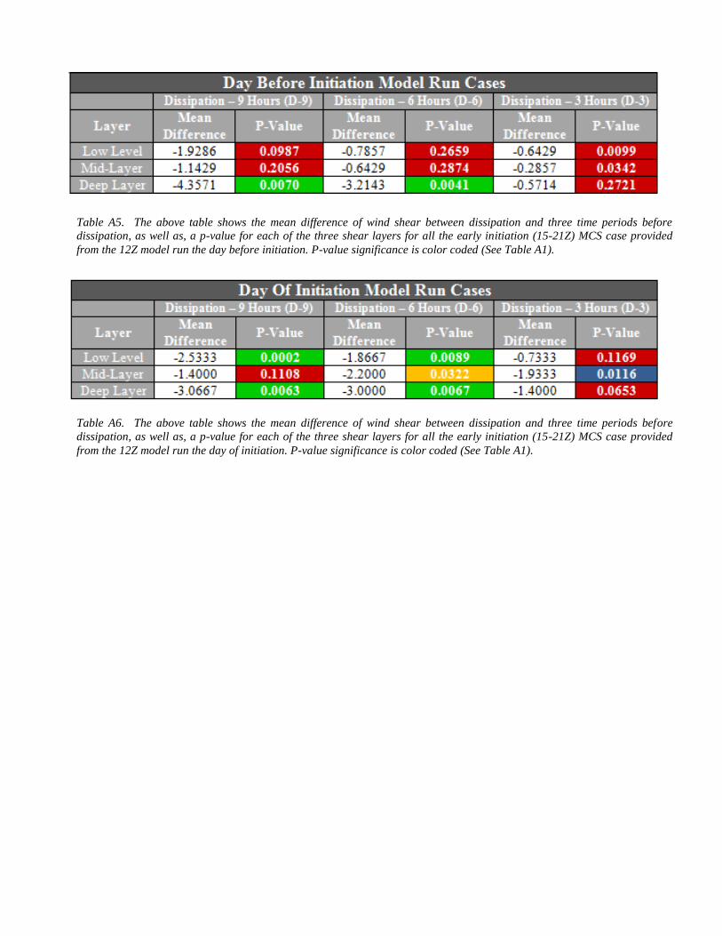
Table A5. The above table shows the mean difference of wind shear between dissipation and three time periods before

dissipation, as well as, a p-value for each of the three shear layers for all the early initiation (15-21Z) MCS case provided

from the 12Z model run the day before initiation. P-value significance is color coded (See Table A1).

Table A6. The above table shows the mean difference of wind shear between dissipation and three time periods before

dissipation, as well as, a p-value for each of the three shear layers for all the early initiation (15-21Z) MCS case provided

from the 12Z model run the day of initiation. P-value significance is color coded (See Table A1).