NASA Contractor Report 2938

Acoustic Analysis

Emission of Fiber

Spectral Composi

Failure Mechanisms

Dennis M. Egan and James H. Williams, Jr.

CONTRACT NSG-3064 JANUARY 1978

https://ntrs.nasa.gov/search.jsp?R=19780007238 2018-06-11T06:57:46+00:00Z

NASA Contractor Report 2938

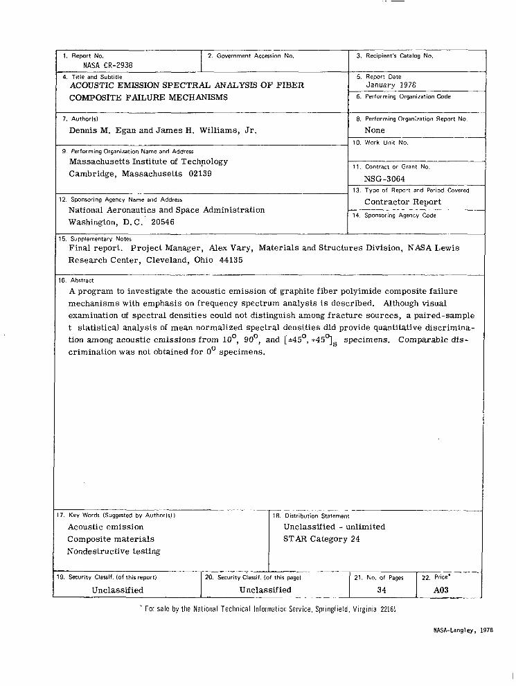
Acoustic Emission Spectral Analysis of Fiber Composite Failure Mechanisms

Dennis M. Egan and James H. Williams, Jr.

Massachusetts Institute of Technology Cambridge, Massachusetts

Prepared for Lewis Research Center under Contract NSG-3064

National Aeronautics and Space Administration

Scientific and Technical Information Office

1978

INTRODUCTION

One of the major goals of researchers in acoustic emission (AE)

is to be able to characterize AE sources and material failure mechanisms.

AE signal characteristics such as energy, event and oscillation counts,

rise and decay times, amplitude distribution, and spectral frequency

distribution may be related to the strain waves which are generated by

the source. Spectral frequency analysis is among the more promising

techniques for assisting the characterization of AE sources.

Graphite fiber polymeric composites comprise a group of modern

materials which combine high specific strength and stiffness to an extent

unattainable in most conventional metals. The primary AE source

mechanisms during composite deformation are (1) fracture of fiber,

(2) fracture of matrix, (3 ) fiber-matrix debonding, ( 4 ) relaxation of

fibers if they fracture, and (5) fiber pull-out against friction during

composite rupture. Because some of these failure modes may be structurally

more important than others and because graphite fiber polymeric composites

often fail in a brittle manner, a knowledge of the source mechanism is

more than academic.

The work reported here is a limited part of an overall program to

study the AE characteristics of graphite fiber polymeric composites. The

purpose of this paper is to illustrate the use of a particular statistical

analysis procedure which may be useful in establishing quantitative AE

spectral analysis measures which can distinguish specimens exhibiting

1

different predominant failure mechanism, and thus distinguish the

different source mechanisms.

2

ACOUSTIC . ~~ ~~ ~ -~ EMISSION SPECTRAL ANALYSIS OF FIBER COMPOSITES

Review o f L i t e r a t u r e - An ex tens ive review and summary o f t h e l i t e r a t u r e r e l a t i n g t o

t h e AE moni tor ing of f iber composi te materials a n d s t r u c t u r e s were con-

ducted by Williams [l]. For t he pu rposes o f t h i s pape r , t he p rev ious

work on AE s p e c t r a l a n a l y s i s o f f i b e r c o m p o s i t e s w i l l be b r ie f ly rev iewed.

In observing the acoust ic emission f rom graphi te epoxy specimens,

Mehan and Mul l in [2 ] s t a t ed t ha t acous t i c even t s occu r red i n t he f r equency

range below 20 H z , a n d t h a t e a c h f a i l u r e mechanism had a d i f f e r e n t

charac te r i s t ic s igna ture . Speake and Cur t i s [ 3 ] repor ted a wide spectrum

of 30-130 kHz w i t h several in t e rmed ia t e d i sc re t e f r equenc ie s fo r no tched

g r a p h i t e r e i n f o r c e d p l a s t i c s a n d a spectrum of O(dc)-70 kHz w i t h i n t e r -

med ia t e d i sc re t e f r equenc ie s fo r wa i s t ed spec imens o f t he same material.

They observed that higher frequency components became more apparent as

specimen rupture w a s approached but that no apparent change in the dominant

f requencies occur red . When these g raphi te composi tes were subjec ted

t o t o r s i o n , s p e c i m e n s w i t h t y p e I f ibers p roduced a broad spectrum

up t o 500 kHz and those with type I1 f ibers p roduced f requencies up t o

1 MHz. I n t h e t y p e I f iber composi tes , the dominant f requencies were i n

t h e 0-100 kHz range a t t w i s t angles less than 90" a n d s h i f t e d t o t h e 100-

325 kHz r a n g e f o r t w i s t a n g l e s g r e a t e r t h a n 90". It w a s sugges t ed t ha t

t h e s h i f t i n f r e q u e n c y w a s d u e t o either a change in t he p redominan t

f a i l u r e mechanisms o r changes i n t h e specimen resonance due t o t h e l a r g e

3

deformations.

Fiber fracture was reported by Mullin and Mehan [4] to have

dominant frequencies at 0.6 and 3.2 kHz for high fiber volume fraction

glass epoxy composites; whereas, Speake and Curtis [3] found the tensile

failure of glass rovings to produce a broad-band spectrum between 0-125

H z plus discrete frequencies at 185 and 225 kHz. Takehana and Kimpara [5]

gave a spectrum of 300 Hz-20 kHz with a dip near 2 kHz for polyester

reinforced with several types of glass rovings. During the pressurization

phase of burst-tests of glass filament wound Polaris chambers,

Green et al. [6,71 obtained a spectrum between 2 and 26 kHz.

Mehan and Mullin [2,4] further showed that different AE signatures

were produced for fiber fracture, matrix fracture and debonding in boron

epoxy composites and that all were in the range from 0.5-16 kHz. Low

fiber volume fraction composites had discrete frequencies in the 0.6-6 kHz

range with dominant frequencies at 1, 2 . 2 and 3 kHz, whereas high fiber

volume fraction composites produced a dominant frequency of 4.7 kHz.

Pipes et al. [8] reported that the spectral content of the AE

from boron aluminum composites that deformed primarily by transverse

tension was unaffected by using two different transducers with a 0.1-0.3

MHz filter and a 0.1 MHz-Hp filter, respectively. On the other hand,

specimens that deformed with large inplane shear produced quite different

spectra for the same transducer-filter substitution. We interpret these

results to suggest that the AE due to transverse tension contained fre-

quencies which were primarily in the 0.1-0.3 MHz bandwidth whereas those

due to inplane shear contained significant frequencies beyond 0.3 MHz.

4

. Reporting . -. " . . . and Statistical Analysis

As observed in [l], the AE results contained in the AE spectral

analysis literature are largely qualitative even though quantitative

measures are often presented. This is primarily due to two reasons:

(1) The reporting of the AE research is often not

sufficiently complete to allow quantitative com-

parisons of data from different sources; and

(2) Few generally accepted data analysis and inter-

pretation techniques exist within the AE community.

The requirements suggested by the first of these reasons can be met by

the adherence to an AE checklist as recommended by Williams [l]. In

regards to the second reason, it should be noted that even within a

single specimen, an incremental change in stress may result in a number

of AE events, some of which may initiate from different sources. Thus,

it is extremely unlikely that any direct comparison between a single AE

event and another AE event will enable source or mechanism discrimination.

Therefore, if groups of AE events are treated as random data and are

statistically analyzed, it may be possible to identify group characteristics

which enable source or mechanism discrimination. We believe that such an

approach has not been used for AE spectral analysis of composites and it

is the results of such an effort that we report in this paper.

5

EXPERIMENTAL EQUIPMENT, SPECIMENS AND ~ ~ PROCEDURES " .

Equipment

An FC-500 (Acoustic Emission Technology, Inc.) wide-band trans-

ducer was used. The vendor calibration of the transducer displayed a

nearly flat response over the frequencies 1 2 5 kHz to 2 MHz. The trans-

ducer's sensitivity over this range was approximately-85 dB(re l V / v Bar).

The transducer was held on the specimen with two rubber bands at a con-

tact force of about 15N, and generally coupled with AET-SC6 viscous resin,

The transducer's output was preamplified by6GdB and bandpass filtered

between 125 kHz and 2 MHz. The filter had a 24 dB/octave roll-off on

each side of the passband. A signal processor (AET Model 201) provided

an additional 4 0 dB amplification, and contained the voltage threshold

setting which was generally maintained at 0.7V. Amplified AE signals

were recorded on a video tape recorder (AET-modified Sony AV-3650) which

exhibited a flat reproduction response between 100 kHz and 2 MHz. A

spectral analyzer (Hewlett Packard Model 8557 A) was used to monitor the

system's background noise during testing and to perform the AE spectral

analysis. Data were recorded on an X-YY recorder (Hewlett Packard Model

7046 A). An Instron Universal Testing Machine (89 ,000 N rating) was used

to tensile load the specimens at a displacement rate which was generally

2.15 x 10-4m/sec.

6

Specimens

The study of failure mechanisms can be facilitated by the choice

of specimens in which one or two such mechanisms predominate. Four types

of uniaxial tensile specimens were selected: O o , loo and 90" unidirec-

tional (as measured relative to the tensile loading axis), and [+45", -

- +45OIs. The specimens were cut from laminates of AS-1 graphite fibers

(Hercules) in a PR-288 polyimide resin (3M Co.). The fiber volume fraction

was 0 .52 .

Spectral Analysis Procedures

AE generated just prior to each specimen's rupture were spectrally

analyzed in an attempt to identify any characteristic spectral signatures.

The taped records of each AE event were replayed on the video recorder

as a periodic gated signal. The resulting signal was input into the

spectral analyzer which was operated between 125 kHz and 1 MHz (swept at

20 kHz/sec), with a maximum resolution of 10 kHz. (No discernable data

were observed above 1 MHz.)

It is important to note that each recorded AE event was actually

superposed onto some level of background noise. Thus, we were motivated

to attempt to separate the spectrum of the AE event from the spectrum of

the background noise upon which the AE event spectrum was superposed.

Assuming that an AE event and the background noise were independent

random variables with no correlation, the "separation" of the AE event's

spectrum from the system background noise spectrum was accomplished as

suggested by Newland [ 9 ] . First, a sample of system background noise was

7

obta ined . This no ise sample was t a k e n j u s t p r i o r t o t h e AE e v e n t t o b e

analyzed and i t w a s t aken fo r an equa l t i m e d u r a t i o n as the ga t ed AE

event . The mean s q u a r e s p e c t r a l d e n s i t y of the system background noise

w a s genera ted , main ta in ing a l l t h e c o n t r o l s e t t i n g s t h e same as those

u s e d f o r p r o c e s s i n g t h e AE event p lus i ts accompanying superposed noise.

The mean squa re spec t r a l dens i ty o f t he AE event was then ob ta ined by

substract ing the system background noise spectrum from the spectrum of

t h e AE event plus superposed noise .

Extens ive de ta i l s o f the equipment , spec imens and test procedures

are given by Egan [ l o ] .

8

RESULTS

Fracture and Typical AE Results

Both fracture characterizations and a number of typical AE measures

were obtained. These included analyses of scanning electron microscopy

of the fracture surfaces, failure modes (Table 11, and ultimate loads

(Table 2). Also, the time-domain character of the AE, AE oscillation

and RMS counts, AE pressure excitation of the transducer, and AE shake-

down (the quasi-irreversibility of AE until the previous maximum historical

load has been exceeded) were investigated and are reported in detail by

Egan [lo].

Spectral Analysis

The normalized spectral energy distribution for each of approxi-

mately 300 AE events were computed and plotted. A s indicated earlier,

these AE events occurred within about 90% of the ultimate load. The

spectra were normalized by dividing the area under each 10 kHz increment

of the AE spectral energy density curve by the total area under the curve

within the bandwidth 125 kHz - 1 MHz. Thus, the units on the ordinate

were dimensionless. Each of these AE event normalized spectra has been \

plotted by Egan [lo].

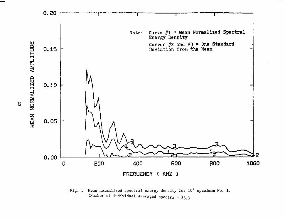
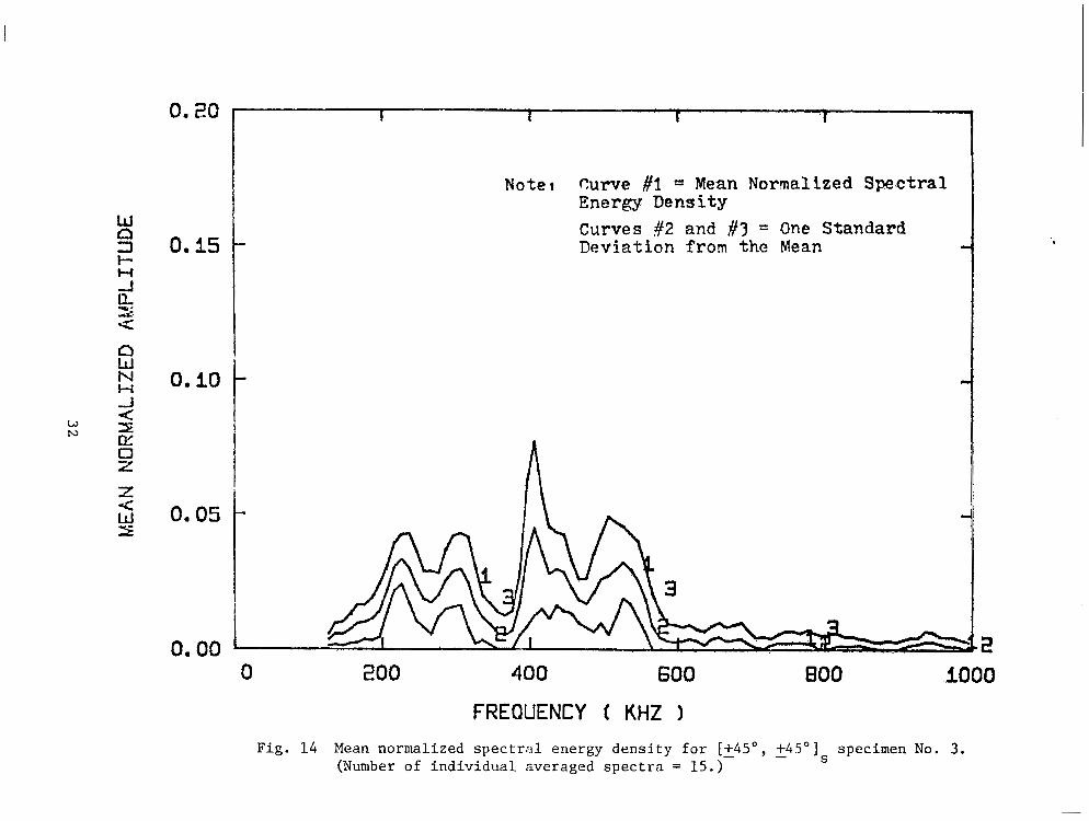
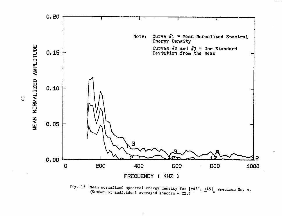
The mean normalized spectral energy distribution for each specimen

was derived as the average of its individual AE event normalized spectral

densities. These are given in Figs. 1 through 15 where the number of

9

averaged individual spectra which were used for each specimen is given

also. The mean normalized spectral energy distribution is labeled ill

and curves 112 and i13 are one standard diviation from the mean. (Note

that negative values were potted as zero for curve #2.)

10

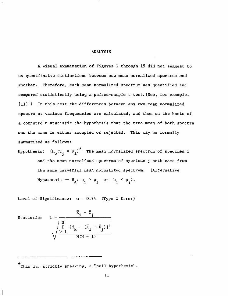
ANALYSIS

A visual examination of Figures 1 through 15 did not suggest to

us quantitative distinctions between one mean normalized spectrum and

another. Therefore, each mean normalized spectrum was quantified and

compared statistically using a paired-sample t test. (See, for example,

[ll].) In this test the differences between any two mean normalized

spectra at various frequencies are calculated, and then on the basis of

a computed t statistic the hypothesis that the true mean of both spectra

was the same is either accepted or rejected. This may be formally

summarized as follows:

Hypothesis: (Ho:w. = pi) The mean normalized spectrum of specimen i *

J and the mean normalized spectrum of specimen j both came from

the same universal mean normalized spectrum. (Alternative

Hypothesis - HA. * Pi ' wj or Pi < wj).

Level of Significance: a = 0.74 (Type I Error)

- xi - iTj Statistic: t =

* This is, strictly speaking, a "null hypothesis".

11

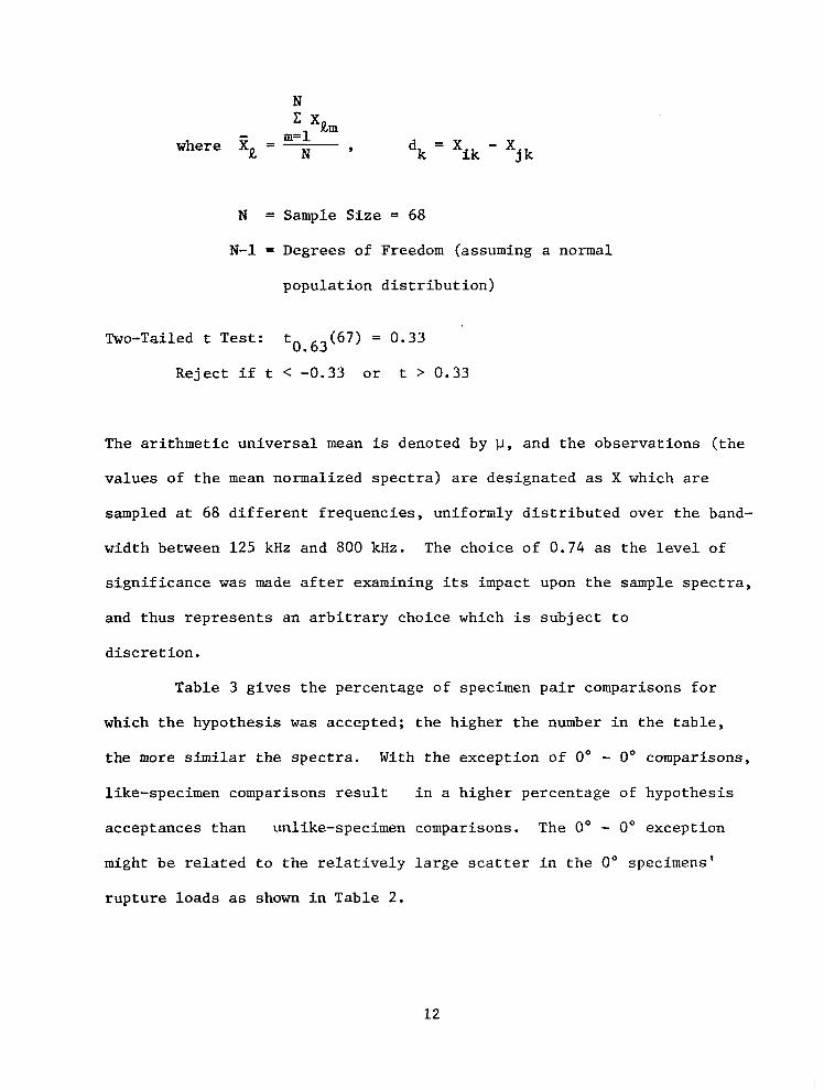
N Xam - m = l where Xa - - N y dk - - Xik - Xj

N = Sample Size = 68

N-1 = Degrees of Freedom (assuming a normal

population distribution)

Two-Tailed t Test: t ( 6 7 ) = 0 . 3 3 0 . 6 3

Reject if t < -0 .33 or t > 0 . 3 3

The arithmetic universal mean is denoted by p, and the observations (the

values of the mean normalized spectra) are designated as X which are

sampled at 68 different frequencies, uniformly distributed over the band-

width between 125 kHz and 800 kHz. The choice of 0.74 as the level of

significance was made after examining its impact upon the sample spectra,

and thus represents an arbitrary choice which is subject to

discretion.

Table 3 gives the percentage of specimen pair comparisons for

which the hypothesis was accepted; the higher the number in the table,

the more similar the spectra. With the exception of 0" - 0" comparisons,

like-specimen comparisons result in a higher percentage of hypothesis

acceptances than unlike-specimen comparisons. The 0" - 0" exception

might be related to the relatively large scatter in the 0" specimens'

rupture loads as shown i n Table 2.

12

CONCLUSIONS AND RECOMMENDATIONS

A program t o i n v e s t i g a t e t h e a c o u s t i c e m i s s i o n o f g r a p h i t e f i b e r

po ly imide composi te fa i lure mechanisms has been conducted. Although a

number of AE measures has been inves t iga ted , AE spec t r a l ene rgy ana lys i s

has been s tudied extensively with an emphasis on the. s ta t i s t ica l d i s -

t i n c t i o n of AE which were genera ted by d i f fe ren t types of composites and

t h u s d i f f e r e n t t y p e s o f f r a c t u r e mechanisms.

Because of the high improbabi l i ty that d i rect comparison of

i nd iv idua l AE e v e n t s c a n r e s u l t i n q u a n t i t a t i v e s o u r c e d i s c r i m i n a t i o n

measures , ind iv idua l AE e v e n t s p e c t r a l d e n s i t i e s were combined t o d e r i v e

mean normalized spectral densi t ies for each specimen. Furthermore, v isual

inspection of even the specimen mean normalized spectral d e n s i t i e s

sugges ts l i t t l e r e g a r d i n g q u a n t i t a t i v e d i s t i n c t i o n s . A paired-sample

t s t a t i s t i c a l c o m p a r i s o n of mean normal ized spec t ra l energy d i s t r ibu t ions

appea r s t o p rov ide quan t i t a t ives d i sc r imina t ion be tween t he AE from l o " , goo and [ + 4 5 O , - +45"Is specimens. For the l imited experimental data

obtained, the paired-sample t tes t could no t ach ieve e i ther conc lus ive

d i s t i n c t i o n o r u n i q u e r e c o g n i t i o n of t h e AE from 0" specimens.

Because of the encouraging results which have been presented, w e

recommend t h a t more s t a t i s t i c a l c h a r a c t e r i z a t i o n s of AE spec t r a be per -

formed. This would include the analysis of more AE e v e n t s t o o b t a i n b e t t e r

estimates o f t he mean normalized spectra , and the use of other types of

s ta t is t ical comparative tests. Also, the composi te dispers ion and

13

attentuation characteristics should be studied in order to develop a

better understanding of the propagation effects on the spectra and ampli-

tudes of AE signals.

14

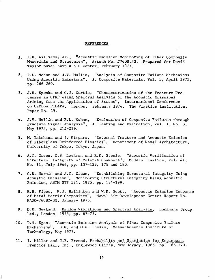
REFERENCES

1. J.H. Williams, Jr., "Acoustic Emission Monitoring of Fiber Composite Materials and Structures" , Artech No. 57600.33. Prepared f o r David Taylor Naval Ship R & D Center, February 1977.

2. R.L. Mehan and J.V. Mullin, "Analysis of Composite F a i l u r e Mechanisms Using Acoustic Emissionsll, J. Composite Materials, Vol. 5, Apri l 1971, pp. 266-269.

3. J . H . Speake and G . J . Cur t i s , "Charac t e r i za t ion of the F rac tu re P ro - cesses i n CFRP us ing Spec t ra l Analys is o f the Acous t ic Emiss ions Ar is ing f rom the Appl ica t ion of S t ress" , In te rna t iona l Conference on Carbon F i b e r s , London, February 1974. The P l a s t i c s I n s t i t u t i o n , Paper No. 29.

4. J.V. Mullin and R.L. Mehan, "Evaluation of Composite Failures through Frac ture S igna l Analys is" , J. Test ing and Evaluat ion, Vol . 1, No. 3, May 1973, pp. 215-219.

5. M. Takehana and I. Kimpara, " In te rna l Frac ture and Acous t ic Emiss ion of Fiberglass Reinforced Plastics' ' , Department of Naval Architecture, Universi ty of Tokyo, Tokyo, Japan.

6. A.T. Green, C.S. Lockman and R.K. Steele, l rAcous t i c Ver i f i ca t ion of S t r u c t u r a l I n t e g r i t y o f P o l a r i s Chambers'', Modern P l a s t i c s , Vol. 41 , No. 11, Ju ly 1964 , pp. 137-139, 178 and 180.

7. C.R. Morais and A.T. Green , "Es tab l i sh ing S t ruc tura l In tegr i ty Us ing Acoust ic Emission", Monitor ing Structural Integri ty Using Acoust ic Emission, ASTM STP 571, 1975, pp. 184-199.

8. R.B. P ipes , N.J. B a l l i n t y n and W.R. Scott , "Acoustic Emission Response of Metal Matrix Composites", Naval A i r Development Center Report No. NADC-76082-30, January 1976.

9. D.E. Newland, Random Vib ra t ions and Spec t r a l Ana lys i s , Longmans Group, Ltd. , London, 1975, pp. 67-73.

10. D.M. Egan, "Acoustic Emission Analysis of Fiber Composi te Fai lure Mechanisms", S.M. and O.E. Thes i s , Massachuse t t s In s t i t u t e o f Technology , May 19 7 7.

11. I. Miller and J . E . F reund , P robab i l i t y and S t a t i s t i c s fo r Eng inee r s , P r e n t i c e Hall, Inc . , Englewood C l i f f s , New Jersey, 1965. pp. 165-170.

15

Table 1

Fracture Modes of Graphite Fiber Polyimide

Composite Specimens

Specimen Type Fracture Mode

Fiber fracture, fiber-matrix debonding with fiber pullout,

tensile fracture of matrix.

Intralaminar shear fracture of matrix.

rl (d C d c, 0 al d k a d G P

0 shear fracture of matrix, and

loo

O0 I goo Tensile fracture of matrix.

[+45" - y + 4 5 O 3 Shear and tensile intralaminar fracture of matrix followed by delamination and fiber fracture.

b

16

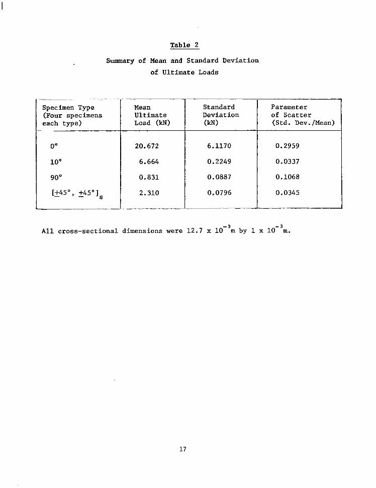
Table 2

Summary of Mean and Standard Deviation

of Ultimate Loads

-. ~~ ~~ -~

Specimen Type (Four specimens each type)

O0

loo

90"

[+45", 245' 1 -

Mean Ultimate Load (kN)

20.672

6.664

0.831

2.310

Standard Deviation

6.1170

0.2249

0.0887

0.0796

Parameter of Scatter (Std. Dev./Mean)

0.2959

0.0337

0.1068

0.0345

A l l cross-sectional dimensions were 12.7 x 10-3m by 1 x 10-3m.

17

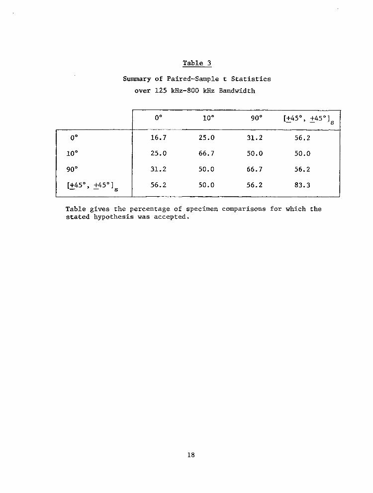
Table 3

Summary of Paired-Sample t S t a t i s t i c s

over 125 kHz-800 lcHz Bandwidth

0"

10"

90"

[+45", - +45OIs

O0 10" 90" [+45", - 245" I s

16.7

25.0

31.2

56.2

25.0

66.7

50.0

50.0

~

31.2

50.0

66.7

56.2

50.0

56.2

56.2 83.3

18

1

I I

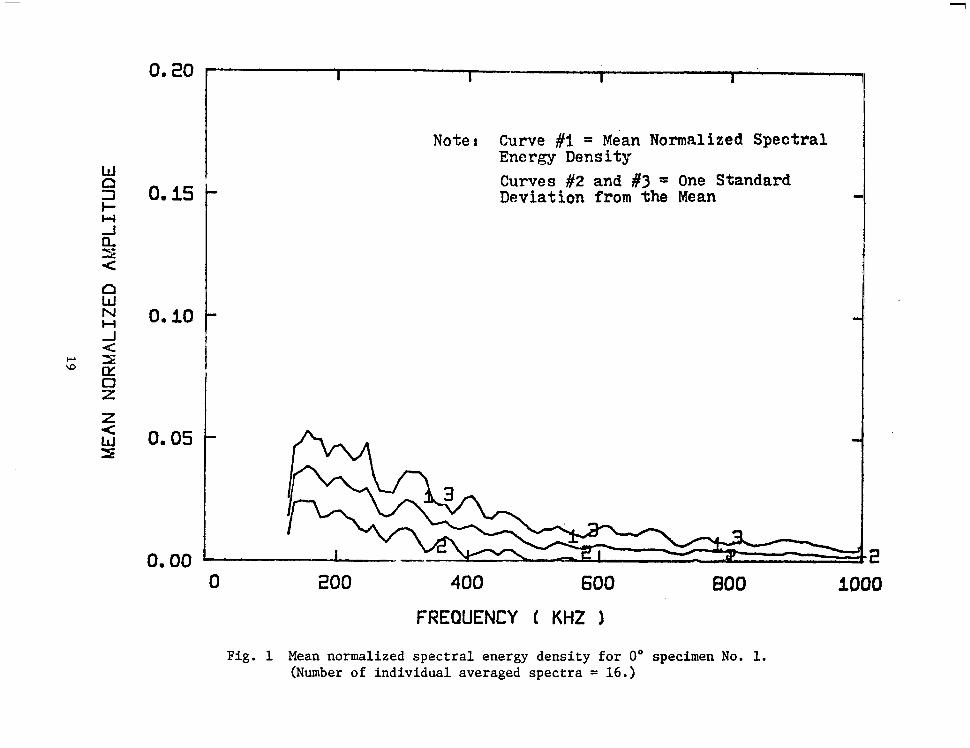
Note: Curve #l = Mean Normalized Spectral Energy Density

0. is

0.10 I o m 05

Curves #2 and #3 = One Standard Deviation from the Mean

om00 0 200 400 600

FREOUENCY ( KHZ 1

BOO 1000

Fig. 1 Mean normalized spectral energy density for 0" specimen No. 1. (Number of individual averaged spectra = 16.)

0.20 I I c 1

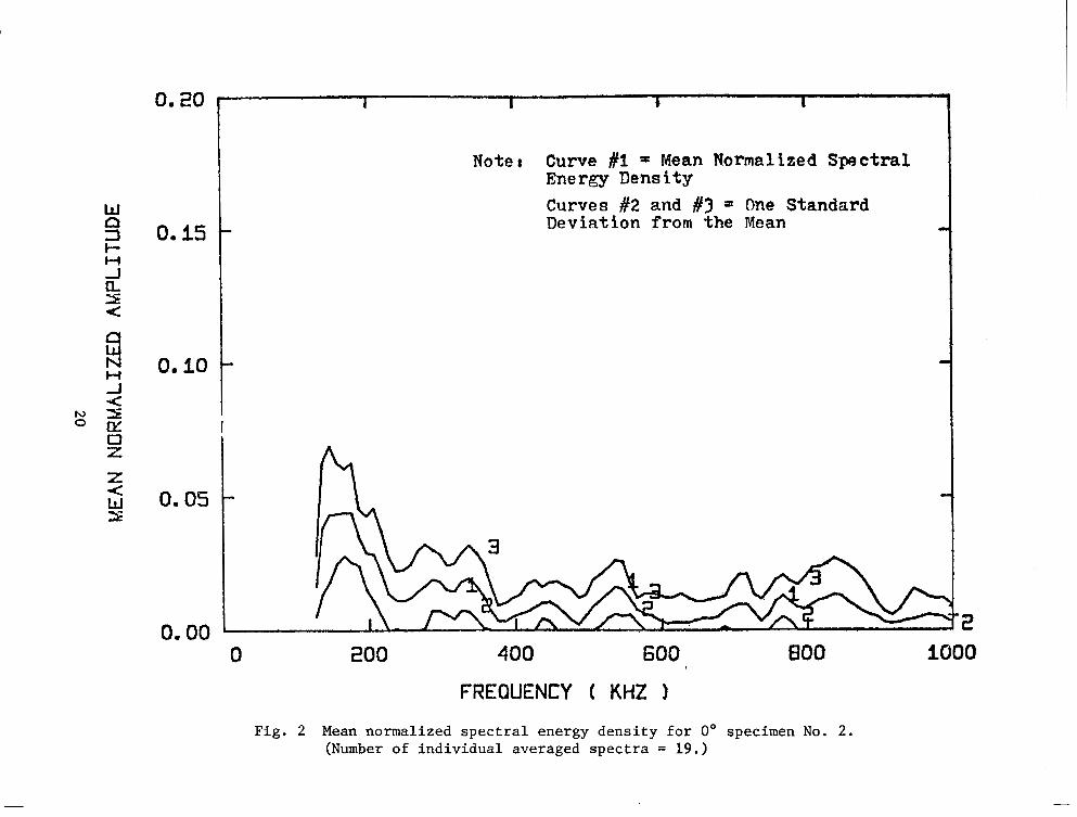
Note: Curve #l = Mean Normalized Spectral Energy Density Curves #2 and #3 = One Standard Deviation from the Mean

0.05

0.00 2 0 200 400 600 800 1000

FREQUENCY ( KHZ 1

Fig. 2 Mean normalized spectral energy density for 0' specimen No. 2. (Number of individual averaged spectra = 19.)

0.20

0.15

0.10

0.05

0.00

I I I I

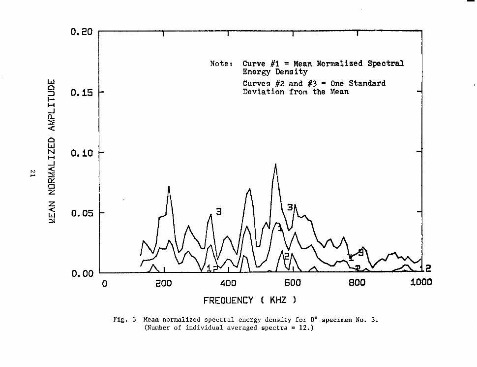
Note; Curve #t = Mean .Normalized Spectral Energy Density Curves #2 and #3 = One Standard Deviation from the Mean

.2 0 200 400 600 BOO

FREQUENCY ( KHZ 1

Fig. 3 Mean normalized spectral energy density for 0' specimen No. 3. (Number of individual averaged spectra = 12.)

0.20 ' I I I I

0.10 -

0.05 -

i

Note: Curve #l = Mean Yormalized Spectral Energy Density Curves #2 and #3 = One Standard Deviation from the Mean

I\\ n3

0.00 1 0 200 400 600 eo0 io00

FREQUENCY ( KHZ 1

Fig. 4 Mean normal ized spec t ra l energy dens i ty for 0" specimen No. 4 . (Number of ind iv idua l averaged spec t ra = 2 3 . )

Om 20

0.15

0.10

O m 05

O m 00

.

I

Note I Curve #I = Mean Normalized Spectral Energy Density Curves #2 and #3 = One Standard Deviation from the Mean

-2 0 200 400 600 BOO 1000

FREQUENCY t KHZ 1

0.20

0. is

0.10

0. os

0.00

Note: Curve #1 = Mean Normalized Spectral Energy Density Curves #2 and #3 = One Standard Deviation froln the Mean -

0 200 400 600 800 1000

FREQUENCY ( KHZ 1

Fig. 6 Mean normalized spectral energy densi ty f o r 10' specimen No. 2. (Number of ind iv idua l averaged spec t ra = 20.)

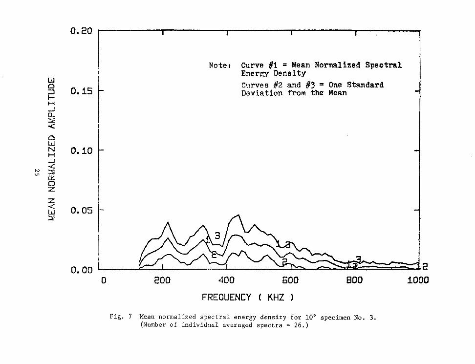
0.20 * I I 1 I

Note: Curve #l = Mean Normalized Spectral I I Energy Density

0.15

0.10

0.05

0.00

Curves #2 and #3 = One Standard Deviation from the Mean

I

4 2 0 200 400 600 800 io00

FREQUENCY ( KHZ I

F ig . 7 Mean n o r m a l i z e d s p e c t r a l e n e r g y d e n s i t y f o r 10' specimen No. 3. (Number of i n d i v i d a a l a v e r a g e d s p e c t r a = 2 6 . )

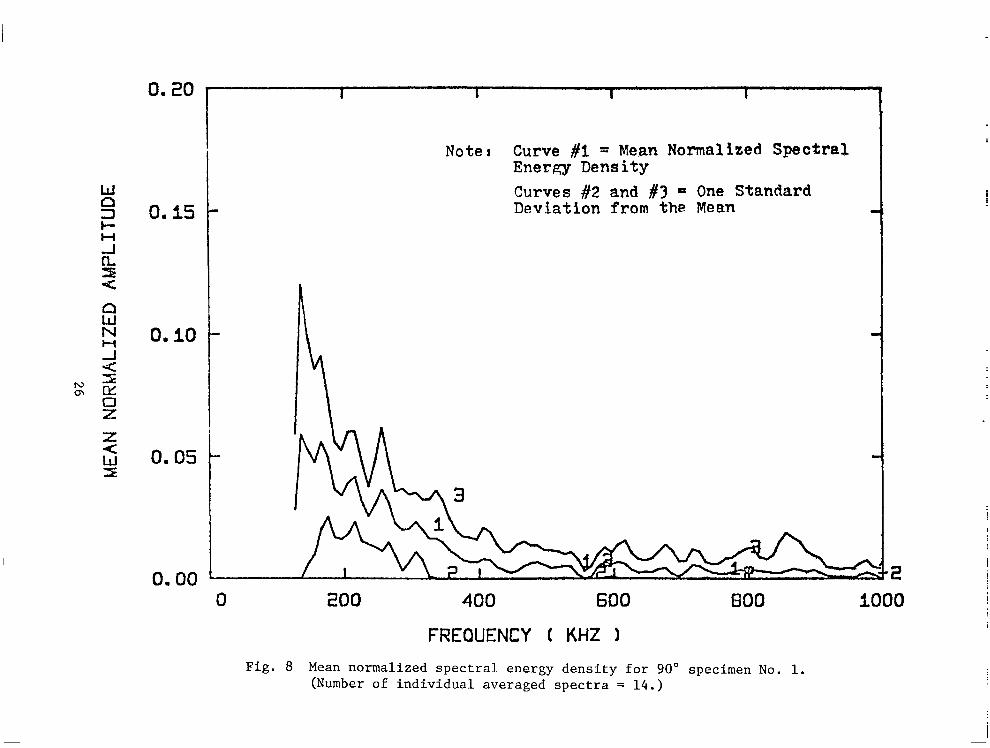
0. 20 I I I I

Note t Curve #i = Mean Normalized Spectral Energy Density Curves #2 and #3 = One Standard Deviation from the Mean

0.00 1 -2 0 200 400 6130 BOO 1000

FREQUENCY KHZ 1 Fig. 8 Mean n o r m a l i z e d s p e c t r a l e n e r g y d e n s i t y f o r 90" specimen No. 1.

(Number of i n d i v i d u a l a v e r a g e d s p e c t r a = 1 4 . )

i

W a J I- H

Om20 1 I I t 1

Om 15

O m 10

0.00

Noter Curve #l = Mean Normalized Spectral Energy Density Curves #2 and #J = One Standard Deviation from the Mean

'2 0 200 400 600 000 1000

FREQUENCY ( KHZ 1

Fig. 9 Mean normalized spectral energy density f o r 90" specimen No. 2. (Number of individual averaged spectra = 10.)

0.20 I I i I

I

0.15 1 0.10 i 0. os

0.. 00

Note; Curve #I = Mean Normalized Spectral Energy Density Curves #2 and #3 = One Standard Deviation from the Mean -

.

-2 0 200 400 600 EO0 io00

FREQUENCY ( KHZ 1 Fig. 10 Mean normalized spectral energy densi ty for 90" specimen No. 3.

(Number of ind iv idua l averaged spec t ra = 1 4 . )

0.20

0.15

0.10

0. os

0.00

I

Note: Curve #I = Mean Noma1 Szed Spec tr&l Energy Density Curves #2 and #2 = One Standard !leviation from the Mean I

0 200 400 600 800

FREOUENCY ( KHZ I

F ig . 11 Mean norma l i zed spec t r a l ene rgy dens i ty f o r 90" specimen No. 4 . (Number of i n d i v i d u a l averaged spectra = 29.)

Om 20

Om 15

0.10

0.05

0.00

Note I Curve #l = Mean Normalized Spectral Energy Density Curves #2 and #3 = One Standard Deviation from the Mean

f

I

I I 02

0 200 400 600 800 io00

FREQUENCY ( KHZ 1 Fig . 1 2 Mean normalj.zed spectraL energy density f o r [ + 4 5 " , + 4 5 " ] specimen No. 1 .

(Number of ind iv idua l averaged spec t ra = 19.)- - s

om 20

0.15

om 10

0.05

0.00

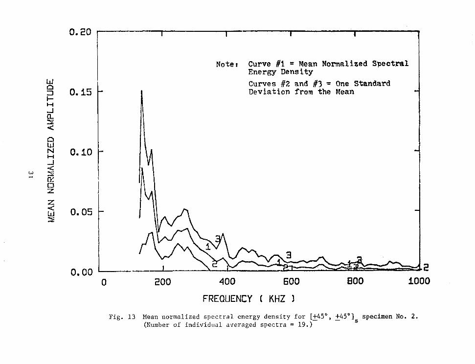
Note: Curve #l = Mean Normalized Spectral Energy Density Curves #2 and #3 = One Standard Deviation from the Mean

.2 0 200 400 600 800 io00

FREQUENCY I KHZ 1

P i g . 13 Mean normalized spectral. energy density f o r [+45", +45O] specimen No. 2. (Number of individual averaged spectra = 19.)-

- S

0.20

0.15

0. io

0.05

0. 00

- ~~~ ~

I - T r ' I

Notes Curve #l = Mean Normalized Spectral Energy Density Curves #2 and #3 = One Standard Deviation f r o n the Mean

0 200 400 600 800 1000

FREQUENCY KHZ 1 Fig. 14 Mean normalized spectral energy density f o r [ +45 ' , 2 4 5 O I s specimen No. 3.

(Number of individual averaged spectra = 15.)-

0.20

O m 15

0.10

Om 05

0.00

I I I . . I . -

Note t

- Curve #I = Mean Normalized Spe.ctra1 Energy Density Curves #2 and #3 = One Standard Deviation from the Mean I

. 0 200 400 600 ' 800

FREQUENCY ( KHZ 1

Fig . 15 Mean normalized spectral energy density for [+45", +45] specimen No. 4. - (Number of individual averaged spectra = 22.)- s

I

1. Report No. 3. Recipient's Catalog No. 2. Government Accession No.

NASA CR-2938 ~-

4. Title and Subtitle ACOUSTIC EMISSION SPECTRAL ANALYSIS OF FIBER COMPOSITE FAILURE MECHANISMS 6. Performing Organization Code

5. Report Date January 1978

7. Author(s)

Dennis M. Egan and James H. Williams, Jr. 8. Performing Organization Report No. I None

10. Work Unit No. 9. Performing Organization Name and Address

Massachusetts Institute of Technology Cambridge, Massachusetts 02139 NSG-3064

1 13. Type of Report and Period Covered

12. Sponsoring Agency Name and Address

National Aeronautics and Space Administration Washington, D. C. 20546

I Contractor Report 14. Sponsoring Agency Code

I 15. Supplementary Notes

Final report. Project Manager, Alex Vary, Materials and Structures Division, NASA Lewis Research Center, Cleveland, Ohio 44135

~~

16. Abstract

A program to investigate the acoustic emission of graphite fiber polyimide composite failure mechanisms with emphasis on frequency spectrum analysis is described. Although visual examination of spectral densities could not distinguish among fracture sources, a paired-sample t statistical analysis of mean normalized spectral densities did provide quantitative discrimina- tion among acoustic emissions from loo, 90°, and [*45', *454, specimens. Comparable dis- crimination was not obtained for 0' specimens.

7. Key Words (Suggested by Author(s) 1 ~___- _ ~ _ . . " L 18. Distribution Statement

Acoustic emission Unclassified - unlimited Composite materials STAR Category 24 Nondestructive testing

~~ - "" 9. Security Classif. (of this report) 20. Security hassif. (of this page)

__ I 21. NO.;; Pages 1 22. 1;: - -. " ". Unclassified Unclassified

~. "" - .~

' For sale by the National Technical Information Service, Springfield, Virginia 22161

NASA-Langl ey , 1978