2012

Analysis of energy saving potentials

in energy generation:

Final results

Report EUR 25409 EN

European Commission

Joint Research Centre

Institute for Energy and Transport

Contact information

Joris Morbee

Address: Joint Research Centre, Institute for Energy and Transport, P.O. Box #2, 1755 ZG Petten, The Netherlands

E-mail: joris.morbee@ec.europa.eu

Tel.: +31 224 56 5442

http://iet.jrc.ec.europa.eu/

http://www.jrc.ec.europa.eu/

This publication is a Reference Report by the Joint Research Centre of the European Commission.

Legal Notice

Neither the European Commission nor any person acting on behalf of the Commission

is responsible for the use which might be made of this publication.

Europe Direct is a service to help you find answers to your questions about the European Union

Freephone number (*): 00 800 6 7 8 9 10 11

(*) Certain mobile telephone operators do not allow access to 00 800 numbers or these calls may be billed.

A great deal of additional information on the European Union is available on the Internet.

It can be accessed through the Europa server http://europa.eu/.

JRC72929

EUR 25409 EN

ISBN 978-92-79-25611-0 (pdf)

ISBN 978-92-79-25612-7 (print)

ISSN 1831-9424 (online)

ISSN 1018-5593 (print)

doi:10.2790/58574

Luxembourg: Publications Office of the European Union, 2012

© European Union, 2012

Reproduction is authorised provided the source is acknowledged.

Printed in the Netherlands

Analysis of energy saving potentials in energy generation:

Final results

TABLE OF CONTENTS

1. Introduction ..............................................................................................................4

2. Methodology and assumptions ..................................................................................4

2.1. Power plant fleet baseline .........................................................................................4

2.2. BAT efficiencies.......................................................................................................4

2.3. Vintage efficiencies ..................................................................................................5

2.4. System efficiency......................................................................................................6

2.5. Load factors ..............................................................................................................7

2.6. Lifetime ....................................................................................................................7

2.7. CO2 emissions...........................................................................................................7

3. Scenarios ..................................................................................................................8

3.1. Scenario 1: Baseline..................................................................................................8

3.2. Scenario 2: Overnight replacement............................................................................8

3.3. Scenario 3: Gradual replacement...............................................................................8

3.4. Scenario 4: PRIMES Reference scenario...................................................................8

3.5. Scenario 4: PRIMES Efficiency scenario ..................................................................9

4. Results ......................................................................................................................9

4.1. Capacity and electricity production ...........................................................................9

4.2. Primary energy savings ...........................................................................................10

4.3. Efficiency ...............................................................................................................13

4.4. CO2 emissions.........................................................................................................14

5. Conclusions ............................................................................................................15

1. INTRODUCTION

Technical developments continue to increase the energy efficiency of power generation

technology, which offers potential primary energy savings. This document provides an estimate

of the primary energy savings that can be achieved by applying best available technologies

(“BAT”) in the power generation sector.

2. METHODOLOGY AND ASSUMPTIONS

2.1. Power plant fleet baseline

For this analysis, the baseline of the current EU-27 power plant fleet has been taken from the

Platt’s PowerVision database1, which contains details such as age and fuel, of every

individual power plant in Europe. The database is current as of the 3rd

quarter of 2010. Table

1 provides an overview of the EU-27 capacity by fuel. For the purpose of this analysis, the

focus is on technologies fuelled by natural gas, hard coal, heavy oil and soft coal / lignite.

These technologies represent 54.6% of all generation capacity in the EU-27. The other large

categories of power plants are nuclear, hydro and wind, but these are not relevant for our

analysis of primary energy savings.

Table 1: Distribution of operating power generation capacity by primary fuel in EU-27. Source: Platt’s

Powervision (Q3 2010).

Primary fuel* Share in

power

generation

capacity

Natural gas 22.0%

Nuclear 16.7%

Hard coal 15.3%

Hydro 15.1%

Heavy oil 9.0%

Soft coal / lignite 8.3%

Wind 8.1%

Other thermal 5.1%

Other 0.4%

Total within scope 54.6%

* Capacity within the scope of the analysis is shown in bold.

In this document, natural gas will be referred to as “Gas”, heavy oil will be referred to as

“Oil”, and hard coal and soft coal / lignite will be lumped together under the term “Coal”.

2.2. BAT efficiencies

The efficiency of the best available technology (“BAT”) for each of the fuels is taken from the

JRC’s Technology Map 20092. The reference efficiencies for Coal and Gas are shown in the

following table.

1 Platts, 2011. PowerVision database, version 2010 Q3. Platts (The McGraw-Hill Companies), New York. 2 European Commission, 2009. 2009 Technology Map of the European Strategic Energy Technology Plan (SET-

Plan). JRC Scientific and Technical Reports. EUR 24117 EN.

Table 2: Reference efficiencies of the BAT power plant per fuel, for 2007 and 2030. Source: Technology

Map 2009.

Fuel BAT Efficiency 2007 Efficiency 2030

Coal Puliverised Coal

Combustion (PCC)

47% 54%

Gas Combined Cycle Gas

Turbine (CCGT)

58% 65%

Estimation of the BAT efficiency for Oil is based on separate assumptions, as will be

explained below.

2.3. Vintage efficiencies

Efficiencies of individual existing power plants are different from the BAT efficiency. Actual

efficiency values of individual power plants are generally confidential. However, a realistic

estimate can be made, based on the year in which the power plant was built, i.e. the “vintage”.

Older power plants typically have lower efficiency. This is evident when looking at the

efficiency of the entire European electricity system per fuel, as shown in the following figure.

The efficiencies in the figure have been calculated using Eurostat data on gross electricity

production and primary energy input per fuel.

Figure 1: EU-27 electricity system efficiencies per fuel 1990-2008. Source: Eurostat.

27.5%

30.0%

32.5%

35.0%

37.5%

40.0%

42.5%

45.0%

47.5%

1990 1995 2000 2005

GAS

GAS 1998-

OIL

COAL

Linear (GAS 1998-)

Linear (OIL)

Linear (COAL)

For Coal and Oil, the efficiency has been steadily increasing throughout the entire period. For

Gas, the efficiency has first increased more rapidly – related to the widespread deployment of

CCGT, followed by an increase at the same pace as Coal and Oil as of 1998. The figure also

contains the linear least-squares best-fit lines for the efficiencies of Coal (1990-2008), Oil

(1990-2008) and Gas (1998-2008). It is very remarkable that the lines are nearly perfectly

parallel, corresponding to an annual increase in efficiency of 0.30 percentage points.

The efficiencies in Figure 1 are system efficiencies, i.e. they refer to the entire electricity

system at a given point in time. This is different from the vintage efficiency, which refers to

the best available technology at the given point in time. However, due to the very consistent

trend of increasing efficiency in the figure, it is reasonable to assume that vintage efficiencies

follow the same trend. This means that a power plant built 10 years ago would have an

efficiency that is 10x0.30%=3.0% lower than a power plant built today. Applying this rule to

the BAT efficiencies listed in Table 2 makes it possible to construct a full time series of

vintage efficiencies of Coal and Gas, both for the past and for the future. Note also that the

increase in efficiency between 2007 and 2030 as projected in Table 2 is fully consistent with

an annual increase of 0.30 percentage points, which further supports our assumption. In order

to account for the significantly lower efficiencies of Gas before 1998, we assume that Gas

vintage efficiencies of plants built before 1998 are an additional 8% lower than what they

would be if only the annual trend of 0.30% is applied.

The ratio between BAT efficiency in 2007 (from Table 2) and system efficiency in 2007

(from Figure 1, corrected for stochastic fluctuations) is 1.3 both for Coal and for Gas. It is

therefore reasonable to assume that the same holds for Oil, which allows for the completion of

the time series of vintage efficiencies. The full time series 1960-2030 are shown in the

following figure.

Figure 2: Assumed vintage efficiencies for power plants built from 1960 to 2030, for different fuels.

0%

10%

20%

30%

40%

50%

60%

70%

1960 1970 1980 1990 2000 2010 2020 2030

Gas

Oil

Coal

The Eurostat data on which Figure 1 is based, is only for electricity, not for heat. Due to data

availability issues it is difficult to make a reliable comparable graph for combined generation

of heat and power (CHP). Therefore, in this analysis, CHP is not considered separately.

Rather, the primary energy savings resulting from the deployment of best available

technologies in electricity-only generation are computed, and then extrapolated to the entire

electricity system, including CHP. Since the penetration of CHP is relatively limited, as

shown in the Progress Report (deliverable 1.2 in the context of this Administrative

Arrangement), this does not significantly affect the results.

2.4. System efficiency

The assumed vintage efficiencies from Figure 2 are applied to all current power plants

depending on their age. The resulting system efficiency of the total fleet of coal-fired power

plants in 2010 would be 37.5%, which is identical to what would be obtained if the Coal

efficiencies in Figure 1 are extrapolated to 2010. For Oil and Gas however, there are

differences between the actual system efficiency (as seen in Figure 1) and the system

efficiency obtained when applying the vintage efficiencies of Figure 2 to the current fleet.

There could be several reasons for this. Most notably, Gas and Oil plants are often operated

only during peak-load, which leads to significant ramp-up and ramp-down time, as a result of

which the power plant is only operating at maximum efficiency during part of the time. To

account for this, a downward correction of 3 and 7 percentage points efficiency is applied to

Oil and Gas, plants respectively, when they are integrated in the system.

2.5. Load factors

Primary energy savings depend not only on the efficiency of the various power plants in the

fleet, but also on the load factors of the plants. Using Eurostat data on electricity production

and the power plant capacity data from PowerVision, the following average load factors are

obtained:

Table 3: Average load factors of power plants in EU-27 by fuel. Source: Platt’s Powervision (Q3 2010),

Eurostat.

Fuel Load factor %

Coal 66

Gas 67

Oil 16

In this document it is assumed that the same load factors hold in the future.

2.6. Lifetime

The potential total primary energy savings that can be achieved through the replacement of

older inefficient power plants with BAT power plants, depend on the timing of the

replacement. In one of the scenarios analysed in the next section, it is assumed that power

plants are replaced when the end of their projected lifetime is reached. The 2009 Technology

Map mentions a technical lifetime of 25 and 40 years for Gas and Coal, respectively.

Experience shows that the lifetime of power plants is often extended in practice at a cost far

below the investment cost of a new power plant. This is further supported by the fact that the

European electricity system contains many operating Gas and Coal power plants of more than

25 and 40 years old, respectively. In this analysis, it is assumed that the lifetime of power

plants, after their initial technical lifetime, is extended by 10 years. Lifetime of Oil plants is

assumed to be the same as Coal plants. The assumed lifetimes are summarised in the

following table.

Table 4: Assumed lifetimes of power plants by fuel.

Fuel Lifetime

Years

Coal 50

Gas 35

Oil 50

2.7. CO2 emissions

Specific CO2 emissions per fuel are taken from the 2006 IPCC Guidelines for National

Greenhouse Gas Inventories3:

3 IPCC, 2006. 2006 IPCC Guidelines for National Greenhouse Gas Inventories. Volume Energy, Chapter 2:

Stationary Combustion.

Table 5: CO2 emissions per fuel.

Fuel CO2 emissions from

combustion t / TJ

Coal* 98.3

Gas 56.1

Oil 74.1

* The value for anthracite is used.

3. SCENARIOS

Four scenarios are studied in the remainder of this document.

3.1. Scenario 1: Baseline

The Baseline scenario assumes that the current power plant fleet is maintained in its current

condition until 2030. This is obviously not a realistic scenario, since power plants are ageing

and many power plants will need to be replaced in the next 20 years. The scenario therefore

serves only as a theoretical baseline against which the other scenarios can be compared.

3.2. Scenario 2: Overnight replacement

This scenario assumes that the 2010 power plant fleet is replaced overnight with the best

available technologies in 2010. Coal capacity is replaced with BAT Coal capacity, Gas

capacity with BAT Gas capacity, and Oil capacity with BAT Oil capacity. Again, this is

obviously not a realistic scenario, but it provides a benchmark for the primary energy savings

that can be achieved.

3.3. Scenario 3: Gradual replacement

In this scenario, capacity is gradually replaced as and when its lifetime, according to Table 4,

is reached. As in Scenario 2 – “Overnight replacement” – capacity is replaced on a like-for-

like basis, i.e. Coal capacity is replaced by Coal capacity and so on. The efficiency of the new

plant depends on the vintage efficiency applicable to the year in which the replacement is

carried out. The vintage efficiencies are taken from Figure 2. Consequently, power plants that

are replaced later in time, will be replaced by more efficient power plants than power plants

that are replaced earlier in time.

3.4. Scenario 4: PRIMES Reference scenario

This scenario is taken from the EU Energy Trends to 2030 – Update 20094. In a model such

as PRIMES, the replacement of power plants is determined from a broader economic

perspective, rather than the heuristic rules of the previous scenarios. Power plants are replaced

when it is optimal for the power plant owners to do so, subject to emissions reductions and

other constraints. The fuel of the new power plant is not necessarily the same as the old one,

4 Capros P, Mantzos L, Tasios N, De Vita A, Kouvaritakis N, 2010. EU energy trends to 2030 - Update 2009.

Publications Office of the European Union, Luxembourg.

and the total capacity of fossil-fuel power plants may increase or decrease. For example, a

large increase in renewables (e.g. solar, wind) may lead to lower thermal capacity. Hence,

even without efficiency improvements, there would be some primary energy savings. Care

must therefore be taken when comparing the PRIMES results with the other scenarios.

3.5. Scenario 4: PRIMES Efficiency scenario

This scenario is taken from simulations performed for DG ENER by the PRIMES team. The

same comments apply as for the PRIMES Reference scenario

4. RESULTS

4.1. Capacity and electricity production

By construction, the total power generation capacity in Coal, Gas and Oil is constant over

time in scenarios 1 (“Baseline”), 2 (“Overnight”) and 3 (“Gradual”). The total capacity is 364

GW, of which 156 GW Coal, 132 GW Gas, and 76 GW Oil. Since load factors are assumed

constant, power generation is also constant, at 1781 TWh per year, i.e. a total of 35611 TWh

over the entire period 2011-2030.

By contrast, as mentioned before, power generation capacity and load factors, and hence

electricity production, are not constant over time in scenarios 4 and 5 (“PRIMES Ref” and

“PRIMES Eff”, respectively). The following two figures compare the constant electricity

production mix of scenarios 1/2/3 with the mix projected by the two PRIMES scenarios,

respectively. In the PRIMES Reference scenario, electricity generation from fossil fuels

exhibits a declining trend, decreasing at 0.4% per year on average. The decline is most

pronounced for Oil, which declines at 3.0% per year on average. In this PRIMES Reference

scenario, the share of fossil fuels in power generation declines from 53% in 2010 to 40% in

2030. The decline in fossil-fuel power generation in PRIMES needs to be taken into account

when comparing with the results of scenarios 1/2/3 in the next section.

Figure 3: Electricity generation from Coal, Gas and Oil in 2010-2030 for the 3 non-PRIMES scenarios, as

compared with the PRIMES Reference scenario [TWh / y].

104 74 70 48 47 40

775 766 749723 758 724

901 911 911845

878858

1781 1751 1730

16161683

1622

Scenarios

1/2/3

2010-2030

PRIMES

2010

PRIMES

2015

PRIMES

2020

PRIMES

2025

PRIMES

2030

Total

Coal

Gas

Oil

In the PRIMES Efficiency scenario, electricity generation from fossil fuels exhibits a

increasing trend up to 2020 and a declining trend afterwards. On balance there is an average

decline of 0.1% per year. The decline is most pronounced for Oil, which declines at 1.6% per

year on average. There is actually an increase in power generation from coal. Overall, the

share of fossil fuels in power generation declines from 52% in 2010 to 41% in 2030.Again,

the decline in fossil-fuel power generation in PRIMES needs to be taken into account when

comparing with the results of scenarios 1/2/3 in the next section.

Figure 4: Electricity generation from Coal, Gas and Oil in 2010-2030 for the 3 non-PRIMES scenarios, as

compared with the PRIMES Efficiency scenario [TWh / y].

104 72 74 70 61 52

775734 762 826 823

726

901911

923914 901

921

17811717

17601809 1784

1700

Scenarios

1/2/3

2010-2030

PRIMES

2010

PRIMES

2015

PRIMES

2020

PRIMES

2025

PRIMES

2030

Total

Coal

Gas

Oil

The next table compares electricity generation from fossil fuels in the two PRIMES scenarios

to the value in 2010, expressed in percentage decline.

Table 6: Reduction of electricity generation in 2015-2030 in the two PRIMES scenarios, compared to 2010

[Percent]

Scenario 2015 2020 2025 2030

PRIMES Reference -1.2% -7.7% -3.9% -7.4%

PRIMES Efficiency 2.5% 5.4% 3.9% -1.0%

4.2. Primary energy savings

The following figure shows the evolution of primary energy consumption by Coal, Gas and

Oil power plants in each of the five scenarios. For the Baseline scenario, this value remains

constant by construction. For the Overnight scenario, the consumption shows a sharp drop

initially, due to the sudden introduction of more efficient power plants, after which it remains

constant. The Gradual scenario exhibits a gradual decline, which in 2014 goes below the

Overnight scenario, because the Gradual scenario replaces power plants later, when more

efficient technologies are available. The PRIMES Reference scenario starts from a slightly

higher point (due to differences in calibration parameters) but has overall the same downward

trend as the Gradual scenario. The PRIMES Efficiency scenario has a flat profile up to 2020

(presumable because fuel savings take place outside the power generation sector due to

energy efficiency measures), after which it follows the same downward trend as the Gradual

scenario.

Figure 5: Primary energy consumption of Coal, Gas and Oil in each of the 5 scenarios [Mtoe / y].

250

300

350

400

2010 2015 2020 2025 2030

Scenario 1 - Baseline

Scenario 2 - Overnight

Scenario 3 - Gradual

Scenario 4 - PRIMES

ReferenceScenario 5 - PRIMES

Efficiency

The following table provides an overview of the primary energy savings, defined as the

difference between the actual primary energy consumption of each scenario, and the primary

energy consumption that would have occurred if the initial 2010 value had been maintained

throughout the period. It is interesting to observe that the Gradual scenario has the largest

savings when considering the difference in annual savings between 2010 and 2030, while the

Overnight scenario has the largest total savings over the period. Although the Gradual

scenario implements more efficient technologies, the Overnight scenario has higher savings

because it starts implementation earlier. The savings of the two PRIMES scenarios consist of

two components. The first component represents the savings obtained from deploying more

efficient fossil fuel technologies. This number corresponds to the savings obtained in

scenarios 1-3. The second component – marked with * - represents the additional savings

obtained in the PRIMES scenarios due to the reduction of electricity generation from fossil

fuels in these scenario (i.e. the shift away from fossil fuels), as described in the previous

section. For the PRIMES Reference scenario, the total savings are slightly below the Gradual

scenario, which could already be observed visually in Figure 5. However, only half of this is

due to the deployment of more efficient technologies, the other half being due to the reduction

in electricity generation from fossil fuels. For the PRIMES Efficiency scenario, the annual

savings in 2030 are much lower. Although the savings stemming from efficiency gains are

higher than in the PRIMES Reference scenario (34 versus 28 Mtoe/y), the total savings are

lower due to a lower reduction of electricity generation from fossil fuels. In fact, , the second

component is negative when considering the total over the entire period 2011-2030, because

in the PRIMES Efficiency scenario there is initially an increase in electricity generation from

fossil fuels.

Table 7: Primary energy savings of the 5 scenarios.

Scenario Difference in annual

primary energy

consumption 2010-2030

Total primary energy

savings over the period

2011-2030

Mtoe / y % of 2010

consumption

Mtoe

1 – Baseline 0 0% 0

2 – Overnight 51 14% 1024

3 – Gradual 63 18% 756

4 – PRIMES Reference 28+28*=56 7%+7%*=15% 338+308*=646

5 – PRIMES Efficiency 34+4*=38 9%+1%*=10% 377–210*=167

* Savings marked with * are obtained through reduction of electricity generation from fossil

fuel capacity, rather than through shifting towards more efficient technologies

As mentioned before, the results of the Gradual scenario are obtained by considering the age

and vintage efficiency of every individual power plant in the EU-27, and replacing each

power plant with the BAT as and when its lifetime expires. The results can therefore easily be

broken down to Member State level, as shown in the following table. In absolute terms, the

largest primary energy savings potential is in those Member States with large Coal fleets,

most notably the United Kingdom, Germany and Poland. The annual primary energy savings

potential in relative terms – shown as a percentage in the table – is largest in Latvia, Estonia

and Slovenia. Note again that this analysis is based on the simplifying assumptions described

in Section 2, and that further detailed investigation would be required to confirm the potential,

hence the information provided here should be treated with care.

Table 3: Primary energy savings in Scenario 3 (Gradual), broken down to Member State level.

Member State Difference in annual primary

energy consumption 2010-2030

Total primary energy

savings over the period

2011-2030

Mtoe / y % of 2010

consumption

Mtoe

Austria 0.7 19% 13

Belgium 1.4 20% 17

Bulgaria 1.3 18% 10

Cyprus 0.0 5% 0

Czech Republic 2.9 26% 35

Denmark 0.5 26% 5

Estonia 0.1 30% 1

Finland 0.8 19% 6

France 4.2 20% 55

Germany 7.9 21% 98

Greece 1.0 11% 9

Hungary 1.4 27% 27

Ireland 0.5 9% 6

Italy 6.0 11% 79

Latvia 0.1 31% 3

Lithuania 0.2 28% 3

Luxembourg 0.0 1% 0

Malta 0.0 6% 0

Netherlands 3.4 21% 57

Poland 7.1 20% 76

Portugal 0.1 3% 1

Romania 2.1 22% 18

Slovakia 0.6 27% 10

Slovenia 0.4 30% 4

Spain 3.8 9% 42

Sweden 0.3 19% 3

United Kingdom 16.2 20% 178

Total 63.0 18% 756

4.3. Efficiency

As pointed out above, comparisons of primary energy savings between PRIMES and the other

three scenarios are biased because electricity production is not the same. In the previous

sections, this was addressed by breaking down the primary energy savings from PRIMES into

two components. Another way to study this issue is in Figure 6, where total system

efficiencies (all fuels combined) are shown, i.e. the ratio between electricity produced and

primary energy consumed. The efficiency in the PRIMES scenarios increases a bit less rapidly

than in the Gradual scenario, which is consistent with the previous section, in which it was

shown that the PRIMES scenarios have less savings from efficiency gains. This may be due to

lower assumed BAT efficiency improvements over time, slower replacement rates of power

plants, or other differences in power plant fleet modelling calibration parameters. The

efficiency gains in the two scenarios are very similar to each other. The fact that the PRIMES

Efficiency scenario shows higher absolute savings from efficiency gains (i.e. the first

component in Table 7) compared to the PRIMES Reference scenario, is therefore almost

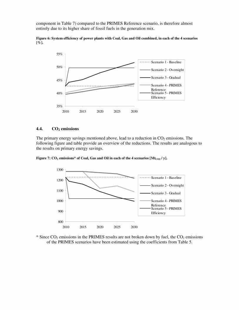
entirely due to its higher share of fossil fuels in the generation mix.

Figure 6: System efficiency of power plants with Coal, Gas and Oil combined, in each of the 4 scenarios

[%].

35%

40%

45%

50%

55%

2010 2015 2020 2025 2030

Scenario 1 - Baseline

Scenario 2 - Overnight

Scenario 3 - Gradual

Scenario 4 - PRIMES

ReferenceScenario 5 - PRIMES

Efficiency

4.4. CO2 emissions

The primary energy savings mentioned above, lead to a reduction in CO2 emissions. The

following figure and table provide an overview of the reductions. The results are analogous to

the results on primary energy savings.

Figure 7: CO2 emissions* of Coal, Gas and Oil in each of the 4 scenarios [MtCO2 / y].

800

900

1000

1100

1200

1300

2010 2015 2020 2025 2030

Scenario 1 - Baseline

Scenario 2 - Overnight

Scenario 3 - Gradual

Scenario 4 - PRIMES

ReferenceScenario 5 - PRIMES

Efficiency

* Since CO2 emissions in the PRIMES results are not broken down by fuel, the CO2 emissions

of the PRIMES scenarios have been estimated using the coefficients from Table 5.

Table 8: CO2 emissions reductions of the 4 scenarios.

Scenario Difference in annual CO2

emissions 2010-2030

Total CO2 emissions

reduction over the period

2011-2030

MtCO2 / y % of 2010

emissions

MtCO2

1 – Baseline 0 0% 0

2 – Overnight 203 17% 4069

3 – Gradual 230 19% 2704

4 – PRIMES Reference 196 15% 2225

5 – PRIMES Efficiency 66 5% 321

5. CONCLUSIONS

The introduction of best available technologies in the current fleet of fossil-fuel power

generation could generate primary energy savings of 14-18% by 2030, compared to primary

energy consumption in 2010.

A gradual replacement of power plants at the end of their lifetime, by the best available

technology could lead to around 750 Mtoe of total primary energy savings over the period

2011-2030. Total CO2 emissions over the period would be reduced by 2.7 Gt. The largest

potential is in Member States with large coal-fired power plant fleets.

These potentials are slightly higher than the PRIMES Reference scenario. In addition, around

half of the potential in the PRIMES Reference scenario is due to a shift away from fossil

fuels, rather than efficiency improvements. The potential is also much higher than the

PRIMES Efficiency scenario. In the latter scenario, the shift away from fossil fuels is much

less pronounced than in the PRIMES Reference scenario.

The results are strongly dependent on the assumptions made, hence care should be taken when

interpreting them.

European Commission

EUR 25409 EN --- Joint Research Centre --- Institute for Energy and Transport

Title: Analysis of energy saving potentials in energy generation: Final results

Author: Morbee, Joris

Luxembourg: Publications Office of the European Union

2012 --- 16 pp. --- 21.0 x 29.7 cm

EUR --- Scientific and Technical Research series --- ISSN 1831-9424 (online), ISSN 1018-5593 (print)

ISBN 978-92-79-25611-0 (pdf)

ISBN 978-92-79-25612-7 (print)

doi:10.2790/58574

Abstract

The introduction of best available technologies in the current fleet of fossil-fuel power generation could generate primary

energy savings of 14-18% by 2030, compared to primary energy consumption in 2010.

A gradual replacement of power plants at the end of their lifetime, by the best available technology could lead to around 750

Mtoe of total primary energy savings over the period 2011-2030. Total CO2 emissions over the period would be reduced by 2.7

Gt. The largest potential is in Member States with large coal-fired power plant fleets.

These potentials are slightly higher than the PRIMES Reference scenario. In addition, around half of the potential in the PRIMES

Reference scenario is due to a shift away from fossil fuels, rather than efficiency improvements. The potential is also much

higher than the PRIMES Efficiency scenario. In the latter scenario, the shift away from fossil fuels is much less pronounced than

in the PRIMES Reference scenario.

The results are strongly dependent on the assumptions made, hence care should be taken when interpreting them.

z

As the Commission’s in-house science service, the Joint Research Centre’s mission is to provide EU

policies with independent, evidence-based scientific and technical support throughout the whole policy

cycle.

Working in close cooperation with policy Directorates-General, the JRC addresses key societal

challenges while stimulating innovation through developing new standards, methods and tools, and

sharing and transferring its know-how to the Member States and international community.

Key policy areas include: environment and climate change; energy and transport; agriculture and food

security; health and consumer protection; information society and digital agenda; safety and security

including nuclear; all supported through a cross-cutting and multi-disciplinary approach.

LB-N

A-2

5409-E

N-N