PNNL-22877

Prepared for the U.S. Department of Energy under Contract DE-AC05-76RL01830

Analysis of Benefits of an Energy Imbalance Market in the NWPP NA Samaan R Schellberg D Warady S Williams R Bayless S Conger R Brush T Gossa M Symonds K Harris J Newkirk C Kalich TB Nguyen M Rarity P Williams P Damiano C Jin S Wallace M Landauer C Macarthur D Wu J Austin H Owen T Martin R Diao R Noteboom W Morter J Hoerner YV Makarov T Van Blaricom K Haraguchi S Knudsen L Kannberg K McRunnel J Portouw A Johnson T Guo J Apperson K Downey R Link S Dennison-Leonard M Empey S Sorey D Holcomb M Goodenough P Etingov October 2013

PNNL-22877

Analysis of Benefits of an Energy Imbalance Market in the NWPP NA Samaan (PNNL) PM R Schellberg (IPC) D Warady (SMUD) S Williams (BPA) R Bayless (NTTG) TL S Conger (BPA) R Brush (NWE) T Gossa (PGE) M Symonds (BPA) TL K Harris (CG) J Newkirk (PSE) C Kalich (AVA) TB Nguyen (PNNL) M Rarity (PSE) P Williams (BPA) P Damiano (CG) C Jin (PNNL) S Wallace (NTTG) M Landauer (CG) C Macarthur (DGT) D Wu (PNNL) J Austin (PAC) H Owen (CHPD) T Martin (TPWR) R Diao (PNNL) R Noteboom (GCPD) W Morter (SCL) J Hoerner (PSE) YV Makarov (PNNL) T Van Blaricom (SMUD) K Haraguchi (BPA) S Knudsen (BPA) L Kannberg (PNNL) K McRunnel (GCPD) J Portouw (PAC) A Johnson (BPA) T Guo (Energy Exemplar) J Apperson (PAC) K Downey (PAC) R Link (PAC) S Dennison-Leonard (NWPP) M Empey (UAMPS) S Sorey (SMUD) D Holcomb (SMUD) M Goodenough (Powerex) P Etingov (PNNL) October 2013 Prepared for the Northwest Power Pool under Contract DE-AC05-76RL01830 Pacific Northwest National Laboratory Richland, Washington 99352

Executive Summary

The Northwest Power Pool (NWPP) Market Assessment Committee (MC) Initiative, which was officially launched on March 19, 2012, set out to explore a range of alternatives that could help the Balancing Authorities and scheduling utilities in the NWPP area address growing operational and commercial challenges affecting the regional power system.

The MC formed an Analytical Team with technical representatives from each of the member Balancing Areas in the NWPP and with staff of Pacific Northwest National Laboratory (PNNL). This Analytical Team was instructed to conduct extensive studies of intra-hour operation of the NWPP system in the year 2020 and of the NWPP region with 14,671 MW of wind penetration. The effort utilized a sub-hourly production cost model (the PLEXOS® computer model) that inputs data from the Western Electricity Coordinating Council (WECC)-wide Production Cost Model (PCM) to evaluate potential production cost savings.

The Analytical Team was given two general options to evaluate. These are the following:

• Energy Imbalance Market (EIM): establishment of an automated, organized NWPP area market for economically supplying energy imbalance within the hour.

• Enhanced Market-Operational Tools (EMT) that might augment or replace an EIM.

The Analytical built on the WECC-wide PCM data from prior work done in the WECC and carried forward the evolution of the original WECC Transmission Expansion Planning Policy Committee (TEPPC) 2020 PC0 data base. A large number of modifications and improvements were made to this case and the data were subjected to extensive review by the team members to improve the model representation of the Northwest (NW). MC meetings that were open to the public were held for interested parties to review and provide input to the study.

Results for the test, base, and sensitivity case studies performed by the MC Initiative Analytical Team indicate that there are a wide range of benefits that could be obtained from the operation of an EIM in the NWPP depending on what assumptions are made. The instructions from the MC were to determine a “minimum high confidence” range of potential benefits. The results for the Base Case indicate that the EIM benefits ranged from approximately $40 million to $70 million in annual savings from the operation of an EIM in the NWPP footprint.

A number of additional relevant sensitivity cases were performed, including low and high water conditions, low and high natural gas prices, and various flexible reserve requirements, resource operations, and amounts of resource capability held back during the preschedule period. Along with the results for the Base Case, the results for these studies yielded EIM benefits that clustered within the range of $70 million to $80 million dollars per year with potential benefits ranging from approximately $125 million to as little as $17 million per year.

Because the design and operation of an EIM could enable participating Balancing Authorities (BAs) to collectively lower the quantity of resources they must carry to meet within-hour balancing needs, a sensitivity case was also performed to analyze the impact that such reductions might have on the benefits from an EIM. The results for this sensitivity case indicate that such reductions could increase the benefits

iii

from the operation of an EIM in the NWPP into the range of approximately $130 million to $160 million per year. Also, a sensitivity case for a WECC-wide EIM was performed with the results indicating that the potential benefits to the NWPP could increase into the range of $197 million to $233 million per year.

While there may be potential reliability benefits from the coordinated dispatch process underlying the operation of an EIM, reliability benefits from an EIM were out of the scope of this study. The EIM benefit analyses that were performed by the Analytical Team are provided in this report. A separate MC working group developed the costs associated with implementing an EIM. These cost estimates will be combined with the benefit results of this study and reported in the MC Final Report.

Modeling Approach:

The approach taken by the Analytical Team to model potential benefits of an EIM focused on quantifying the relative differences between the production costs expected under two different BA operating regimes. These are the following:

a. “Business-as-usual” (BAU) conditions: sub-hourly operations without an energy imbalance market. In this operating regime, a BA dispatches its own resources to meet its own loads and imbalances while holding schedules with other BAs constant over the operating hour.

b. With an energy imbalance market. Assumed BA members in the NWPP EIM operate as a combined virtual Balancing Area to meet the intra-hour imbalances.

For almost all model runs, the Analytical Team designed the BAU and EIM scenarios such that they would be identical in the day-ahead trading, unit-commitment, and scheduling process, as well as through the completion of the same-day hourly scheduling. The divergence in the two cases was in the treatment of intra-hour dispatch.

Under the BAU scenarios, each BA was required to hold the interchange schedules that reflected final day-ahead and hourly scheduling outcomes. Management of intra-hour variability and uncertainty (forecasting errors) associated with load, wind and solar was the responsibility of each individual BA.

In the EIM scenarios, the BAs were allowed to share their collective intra-hour dispatch capabilities without being constrained by their interchange schedules (which were relaxed in the EIM scenarios). These capabilities were only limited by the real-time physical capability of the transmission system and the available generating units that were dispatched according to economic merit.

In order to help mitigate differences and debates caused by differing efficiency assumptions of pre-scheduled trading and contracts, interchange schedules held between Balancing Authorities over the intra-hour real-time period were modeled using the following approach:

1. Known contracts and joint ownership of generating plants were represented.

2. Generating resources in WECC were optimized in the day-ahead unit commitment and hour-ahead scheduling periods with the only obligation for each BA being to carry specified amounts of contingency and balancing reserves. This is equivalent to making the assumption of perfectly effective trading and contracting with perfect information.

These interchange schedules between BAs were held constant during the real-time hourly period in the BAU scenario but were relaxed between NWPP BAs in the EIM scenario. Reserve requirements for

iv

each BA were held constant in both cases, except in one EIM sensitivity case where balancing reserves were calculated for the NWPP footprint. Thus, the approach used in this study purposefully yielded minimum EIM benefits that one can be highly confident the actual EIM benefits will exceed while accounting for the diversity and economic optimization benefits of combining the resource stacks of the BAs. Marginal production costs were used to represent the bidding behavior of the generation bids into the EIM.

In addition, the PCM algorithm assumed that every generator available during a given real-time period would offer into the EIM its entire dispatchable range at its incremental or decremental costs of operation, even though there is no requirement that they do so in actual operations. This assumption is especially relevant for hydroelectric and wind generation, which were assigned incremental costs of zero. Accordingly, the modeling results reflect an essentially “perfect” real-time market with only physical transmission constraints and the machine capability of generators limiting the degree to which online resources could be economically redispatched.

It should be noted that while this assumption may result in somewhat optimistic estimates of the EIM benefits, the assumption of perfect scheduling during the pre-scheduling period results in a more pessimistic estimate of the EIM benefits. Any inefficiency of trading and contracting that occurs in actual operations because of time constraints, unavailability of information, etc. under the BAU scenario will be removed in an EIM, resulting in higher EIM benefits.

One of the more challenging tasks in the process was representing the complex monthly, weekly, hourly and intra-hour “budgeting” process for flexible hydroelectric facilities. This involves considering not just the immediate market value of the generation and the unit capabilities, but also how operational and economic decisions made in one time frame might affect operational capabilities and economic conditions in future time frames while adhering to the required water budget and wind conditions. Modeling limitations in PLEXOS sometimes required the use of phantom “excess hydro1” to solve troublesome 10 minute time segments within the operating hour. This occurred when a time segment was short of resources even though the time segments surrounding the troublesome segment had committed thermal energy available, which operators in actual operations would adjust the amounts of hydro and thermal generation dispatched between the time segments to cover such shortages. To more accurately compare the production costs of the cases in this event, the Analytical Team developed an approach external to PLEXOS that values this additional excess hydro generation at the cost of available thermal generation in the surrounding 10 minute segments. This excess hydro generation was valued at two different price levels to provide a range of values for comparative purposes.

For each sensitivity case, two different price levels for the excess hydro generation in both the EIM and BAU scenarios were valued at $42.00 per MWh and $57.50 per MWh. The one exception is that the values for excess hydro generation were adjusted in the high and low natural gas price cases to track the implied heat rates derived from the calculated level of production from gas-fired generation units and the assumed natural gas prices per MMBtu at Henry Hub located near Earth, Louisiana.

1 The phase “excess hydro generation” is shorthand reference alluding to difficulty, within the production cost modeling process, of accurately reflecting how operators of hydroelectric projects must often “budget” production capability across multiple time periods to manage myriad constraints, including available water, effects on downstream operations, and legal obligations to fulfill objectives other than power production (such as flood control and mitigation of environmental impacts).

v

Despite these challenges, the expert economic dispatch analysts who participated in the Analytical Team expressed a reasonable level of confidence in the results while acknowledging the complexities of the modeling process.

Overview of Benefit Range and Sensitivities:

Table ES-1 presents in summary form the characteristics of the Base Case and the key sensitivity cases modeled in PLEXOS. Table ES-2 reports the range of calculated NWPP EIM benefits.

The results in Table ES-2 can be viewed differently depending on the perspective of an individual regarding, among other things, the following:

• Different weights are given to the uncertainty associated with what is necessarily an assumption-driven modeling process,

• Different strategies and positions are taken by entities within the overall NWPP footprint,

• Different levels of urgency exist to find near-term and long-term solutions for the issues described in the problem statement, and

• Different views about how the basic logic for optimizing a thermally based system—often described as a “heat-rate swap”—may actually play out in a market footprint where often some hydro production might displace other hydro production, which is more difficult to capture in a model that assigns zero cost to all hydro production.

vi

Table ES-1. Characteristics of the Base Case and the Key Sensitivity Cases Modeled in PLEXOS

Case Descriptions

Base “Core” Case

Base Case (Minimum Achievable Benefits)

• 95% Confidence Interval (CI) used to calculate balancing reserve (load-following and regulation) requirements for each BA

• Held reserves constant between the EIM and BAU scenarios • Footprint: NWPP EIM • Annual average nominal natural gas price of $5.62 per MMBtu at Henry

Hub in 2020 • 2006 hydro energy used to represent average water (2003 for CA).

Flexible Reserves Requirement

Increased Flex Reserve (99.5% CI) Case

• Increased the CI used to calculate balancing reserve requirements to 99.5% for each BA.

• Held reserves constant between the EIM and BAU scenarios.

Reduced EIM Flex Reserve Case

• Reduced the flex reserve obligation in the EIM scenario (about 40% load-following reduction in comparison with the BAU scenario for the Base Case). Load-following reserves were calculated based on the NWPP EIM footprint being a single entity.

• Day-ahead and hour-ahead commitments and dispatch for the EIM scenario were based on the reduced flex reserve requirements.

Inefficiencies 3% Held-back Case • Reduced by 3% the available hydro energy from flexible hydro plants and the maximum available capacities for thermal plants in the day-ahead and hour-ahead periods, causing more units to be committed.

6% Held-back Case • Reduced by 6% the available hydro energy from flexible hydro plants and the maximum available capacities for thermal plants in the day-ahead and hour-ahead periods, causing more units to be committed.

Footprints WECC-Wide EIM Case

• Changed the EIM footprint to WECC-wide, otherwise the same as the Base Case.

NWPP EIM w/o PAC Case

• Changed the NWPP EIM footprint to exclude PAC, otherwise the same as the Base Case.

Natural Gas Prices

High Gas Price Case • Increased the annual average nominal natural gas price to $8.40 per MMBtu at Henry Hub in 2020.

Low Gas Price Case • Decreased the annual average nominal natural gas price to $3.80 per MMBtu at Henry Hub in 2020.

Hydro Alternatives

High Water Case • Substituted the 2006 hydro energy in the Base Case with 2011 hydro energy to represent high water conditions throughout the WECC.

Low Water Case • Substituted the 2006 hydro energy in the Base Case with 2001 hydro energy to represent low water conditions throughout the WECC.

Hydro Modeling Improvement Case

• Optimized the real-time dispatch in 12-hour increments to better represent the information that hydro schedulers have when making decisions.

• Individual hydro plant units were aggregated into fewer units. • Hydro energy constraints were enforced weekly rather than monthly.

vii

Table ES-2. Range of Calculated NWPP EIM Benefits in 2020 ($million)

Case Description

Valuation of Excess Hydro Generation

Equivalent $42.00 per MWh

Equivalent $57.50 per MWh

Base Base Case (Minimum Achievable Benefits)

$41.2 $70.7

Flexible Reserves Requirement

Increased flex reserve (99.5% CI) case $51.3 $78.0

Reduced EIM Flex Reserve Case $130.6 $158.2

Inefficiencies 3% Holdback Case $71.2 $90.3

6% Holdback Case $113.7 $124.9

Footprints NWPP Savings in WECC-Wide Case (Indicative Only)

$197.0 $233.0

NWPP EIM w/o PAC Case $37.4 $63.2

Natural Gas Prices High Gas Price Case1 $79.4 $122.7

Low Gas Price Case2 $16.7 $34.8

Hydro Alternatives

High Water Case $60.1 $84.9

Low Water Case $17.1 $49.5

Hydro Improvement Case $71.6 $82.2

Parsing the Energy Imbalance Market Benefits from PLEXOS

As requested by the MC Participants, the Analytical Team explored potential approaches for estimating how the EIM benefits calculated by PLEXOS might be allocated (or “parsed”) among the BAs participating in the MC Initiative. Due to limitations in the capabilities of the PCM to accurately compute Locational Imbalance Prices (LIPs) for many periods when there was an overabundance of hydro and wind generation having zero marginal cost, parsing based on the nodal prices estimated by the model was not feasible.

The relative amounts of transactions between the BAs were determined to be representative of the NWPP EIM benefits, as well as the overall reduction in the societal production costs. The Analytical Team ultimately elected to use a methodology that assumed that intra-hour transactions between the BAs

1 Excess hydro energy being valued at higher electricity prices of $62.78/MWh and $85.94/MWh (rather than $42.00/MWh and $57.50/MWh

2 The excess hydro energy being valued at lower electricity prices of $28.40/MWh and $34.80/MWh (rather than $42.00/MWh and $57.50/MWh

viii

in the NWPP EIM would occur only because both parties financially benefit. Therefore, the parsing results should reflect all BAs receiving a share of the societal benefits.

The parsing methodology measured the volume of intra-hour transactions between the BAs in the NWPP EIM and then assumed that the total annual benefits calculated by the PCM would flow to each of the BAs in proportion to their respective shares of the overall transaction volume.

This was the most workable approach the Analytical Team was able to identify, but it yields results that are not necessarily representative of the actual benefits any particular market participant or BA would experience. Actual benefits could be affected by many factors that this methodology could not capture, such as overall market share, market position, shifts in the market, conditions that influence operations and/or performance in competitive markets, congestion, and treatment of transmission usage for energy imbalance transactions.

Moreover, although the parsing process allocated a portion of the gross benefits to each of the BAs in the NWPP EIM, it does not necessarily follow that the calculated benefits would flow to either the operator of that BA or to the load-serving entities within that BA. The parsing results simply reflect the estimated transaction volumes into and out of particular BAs, but they provide no information about which parties within the BA are actually transacting, what they might do with any savings, or the additional earnings they gain through participation in the EIM.

Table ES-3 reports the parsing results for the Base Case with the excess hydro generation being valued at $42.00/MWh.

Table ES-3. Parsed Societal Benefits for the Base Case by BA Participating in the NWPP EIM

Balancing Authority Transaction Volume

Percentage Share of Savings in

k$ AVA 4.77% $1,963 BCTC 17.59% $7,239 BPA 25.77% $10,605 IPC 5.225% $2,148

Mid C 3.385% $1,391 NWMT 3.64% $1,498

PAC 9.85% $4,053 PGN 5.11% $2,103 PSE 5.03% $2,070 SCL 6.90% $2,839

BANC 9.25% $3,807 TIDC 1.84% $757 TPWR 1.33% $547

WAUW 0.32% $132 NWPP 100% $41,152

ix

Acknowledgments

The Pacific Northwest National Laboratory project team and Northwest Power Pool MC EIM/EMT Working Groups would like to express their appreciation to the following people and organizations for their support of this project, their contributions advancing the state of the art of intra-hour analysis and modeling, and for providing the contract support, IT, room and travel scheduling, and all the other tasks necessary for the study to succeed.

NWPP Analytical Team Tasks Leadership Rich Bayless (NTTG) Mark Symonds (BPA) Kevin Harris (CG) Ron Schellberg (IPC) Steven Wallace (NTTG) Jamie Austin (PAC) Debra Warady (SMUD) Sid Conger (BPA) Stan Williams (BPA) Teyent Gossa (PGE) Joshua Newkirk (PSE) Matt Rarity (PSE) Marv Landauer (CG) Pacific Northwest National Laboratory (PNNL) Landis Kannberg Dale King Carl Imhoff Mark Morgan Steve Shankle Rolando Lara Sue Arey Maura Zimmerschied Megan Peters Lorena Ruiz Katie Dickenson Northwest Power and Conservation Council Ben Kujala Bonneville Power Administration (BPA) Rachel Dibble Aimee Higby Columbia Grid Patrick Damiano Katy Roberts

xi

Energy Exemplar Tao Guo Guangjuan Liu David Llewellyn Shami Davis

Northwest Power Pool (NWPP) Sarah Dennison Leonard Jerry Rust

Northern Tier Transmission Group (NTTG) Sharon Helms Western Electricity Coordinating Council Michelle Mizumori Matt Hunsaker Western Governors Association and PUC EIM Jason Marks Travis Kavulla Doug Larson National Renewable Energy Laboratory (NREL) Michael Milligan Kara Clark U.S. Department of Energy (DOE) Charlton Clark Gil Bindewald Larry Mansueti Kevin Lynn

xii

Acronyms and Abbreviations

ACE Area Control Error AECO Alberta Energy Company AESO Alberta Electric System Operator AGC automatic generation control APS Arizona Public Service AVA Avista Corporation BA Balancing Authority BAA Balancing Authority area BANC Balancing Authority of Northern California BAU Business as Usual BCHA British Columbia Hydro and Power Authority BCTC British Columbia Hydro and Power Authority BEPC Basin Electric Power Cooperative BPA Bonneville Power Administration CAISO California Independent System Operator CC combined cycle CCGT combined-cycle gas turbine CI confidence interval CL confidence level COI California-Oregon Intertie CT combustion turbine DA day-ahead DOPD Public Utility District No. 1 of Douglas County, WA EIM energy imbalance market GCPD Public Utility District of Grant County, WA GT gas turbine HA hour-ahead HTC hydrothermal coordination IPC Idaho Power Company IRP Integrated Resource Plan LADWP Los Angeles Department of Water and Power LIP Locational Imbalance Price MC Market Assessment Committee NREL National Renewable Energy Laboratory NW Northwest NWMT NorthWestern Energy

xiii

NWPP Northwest Power Pool OTC Operating Transfer Capability PAC PacifiCorp PCM Production Cost Model PG&E Pacific Gas & Electric PGN Portland General Electric PNNL Pacific Northwest National Laboratory PSC Public Service Company of Colorado PSE Puget Sound Energy PUC Public Utility Commission PUD Public Utility District RPS Renewable Portfolio Standard RT real time SCE Southern California Edison SCL Seattle City Light ST short term TEPPC Transmission Expansion Planning Policy Committee TIDC Turlock Irrigation District TPWR Tacoma Power UC/ED unit commitment/economic dispatch USE unserved energy VGS Variable Generation Subcommittee WAPA Western Area Power Administration WAUW Western Area Power Administration - Upper Great Plains West Region WECC Western Electricity Coordinating Council

xiv

Contents

Executive Summary .......................................................................................................................... iii Acknowledgments .............................................................................................................................. xi Acronyms and Abbreviations ......................................................................................................... xiii 1.0 Introduction ............................................................................................................................. 1.1

1.1 Overview of NWPP MC Activities ................................................................................. 1.1 1.2 Areas of Concern with Prior Studies ............................................................................... 1.2 1.3 Chronology of NWPP MC Cases Performed .................................................................. 1.4

1.3.1 Test Case .............................................................................................................. 1.4 1.3.2 Base Case Development ....................................................................................... 1.4 1.3.3 Sensitivity Cases .................................................................................................. 1.5

1.4 Study Scope of Work ...................................................................................................... 1.5 1.5 Report Structure .............................................................................................................. 1.6

2.0 Base Case Development .......................................................................................................... 2.1 2.1 BA Structure in the Model .............................................................................................. 2.1

2.1.1 Use of Actual WECC BA Structure ..................................................................... 2.1 2.1.2 Modeling of the BANC BA ................................................................................. 2.3 2.1.3 Mid-C BA ............................................................................................................. 2.4

2.2 Load, Wind and Solar Data ............................................................................................. 2.4 2.2.1 Load Data ............................................................................................................. 2.4 2.2.2 Wind and Solar Data ............................................................................................ 2.7 2.2.3 Changes in Wind Energy Allocation for NWPP BAs .......................................... 2.9

2.3 Changes in Thermal Units Data .................................................................................... 2.10 2.3.1 Retirements and Addition of New Units ............................................................ 2.11 2.3.2 Splitting of CC Units .......................................................................................... 2.11 2.3.3 Startup and Variable O&M Costs ...................................................................... 2.12 2.3.4 Ramp Rates Assumptions ................................................................................... 2.12 2.3.5 Must-Run Units in the Model ............................................................................. 2.13 2.3.6 Natural Gas Price Forecast ................................................................................. 2.13

2.4 Hydropower Plant Modeling ......................................................................................... 2.23 2.4.1 Hydropower Plant Modeling in PLEXOS .......................................................... 2.23 2.4.2 Changes in Hydro Generation Plant Modeling .................................................. 2.27 2.4.3 Hydro Plant Ramp Rates Corrections ................................................................ 2.29 2.4.4 Modeling of MidC Hydro Units ......................................................................... 2.29 2.4.5 Development of High and Low Hydro Scenarios .............................................. 2.31

xv

2.5 Network Topology Changes .......................................................................................... 2.31 2.5.1 Bus/BA Ownership ............................................................................................ 2.31 2.5.2 Modeling Out-of-Area Supply ........................................................................... 2.31 2.5.3 Transmission Topology, Constraints, Flowgates and Nomograms .................... 2.33

2.6 Hurdle Rates Assumptions ............................................................................................ 2.34 2.6.1 Hurdle Rates between Regional Markets ........................................................... 2.34 2.6.2 Hurdle Rate within the NWPP ........................................................................... 2.35

2.7 Reserves Modeling ........................................................................................................ 2.37 2.7.1 Contingency Reserves ........................................................................................ 2.38 2.7.2 Balancing Reserves ............................................................................................ 2.38

3.0 Simulation Approach ............................................................................................................... 3.1 3.1 Rules of Production Cost Modeling ................................................................................ 3.1 3.2 Overview of PLEXOS ..................................................................................................... 3.1

3.2.1 PLEXOS Mid-Term (MT) Simulation and Short-Term (ST) Simulation ............ 3.2 3.2.2 PLEXOS SCUC/ED Algorithm ........................................................................... 3.3 3.2.3 PLEXOS 3-Stage Sequential DA-HA-RT Simulations ....................................... 3.4 3.2.4 Soft Constraint Violation Penalties in the Model ................................................. 3.8

3.3 Description of Base Case and Sensitivity Cases ............................................................. 3.8 3.4 Benefits of an EIM Relative to the Efficiency of the BAU ........................................... 3.10 3.5 Methodologies for Parsing the EIM Benefits for Individual BAs in the NWPP ........... 3.11

3.5.1 Using Locational Imbalance Prices (LIPs) to Track Costs and Benefits ........... 3.11 3.5.2 Using Generation Cost Changes vs. Zonal Exchange Changes in Each

10-Minute Period ................................................................................................ 3.12 3.5.3 Alternative Parsing Methods .............................................................................. 3.13 3.5.4 Sub-Zone Parsing ............................................................................................... 3.14

3.6 Modeling Changes Matrix Compared to Previous Studies ........................................... 3.14 3.7 Improvements Made to Prior Base Case ....................................................................... 3.15

3.7.1 Flexible Reserves Derivation and Modeling Approach ..................................... 3.16 3.7.2 Full Energy Market Versus EIM benefits .......................................................... 3.16 3.7.3 Business as Usual (BAU) Representation .......................................................... 3.16 3.7.4 Hydro Modeling ................................................................................................. 3.17

4.0 Simulation Results Analysis ................................................................................................... 4-1 4.1 Comparison of Base Case HA Simulation Results vs. Historical Generation Mix of

Selected NWPP BAs ...................................................................................................... 4-1 4.1.1 BANC Comparison ............................................................................................. 4-1 4.1.2 PacifiCorp Comparison ....................................................................................... 4-8 4.1.3 Portland General Electric Comparison .............................................................. 4-15 4.1.4 Bonneville Power Administration Comparison................................................. 4-21

4.2 Production Cost Results Summary ............................................................................... 4-24

xvi

4.2.1 Base Case (Case 1.86A) .................................................................................... 4-25 4.2.2 Increased Flexible Reserve Case (Case 1.86B) ................................................. 4-31 4.2.3 3% Held-back Case (Case 1.86C) ..................................................................... 4-36 4.2.4 WECC-Wide EIM (Case 1.86D) ....................................................................... 4-41 4.2.5 High Gas Price Case (Case 1.86E) .................................................................... 4-46 4.2.6 Low Gas Price Case (Case 1.86F) ..................................................................... 4-51 4.2.7 Reduced NWPP EIM Flexible Reserve Case (Case 1.86G) .............................. 4-56 4.2.8 NWPP EIM w/o PAC Case (Case 1.86H) ......................................................... 4-62 4.2.9 6% Held-back Case (Case 1.86I) ...................................................................... 4-67 4.2.10 Low Water Case (Case 1.86J) ........................................................................... 4-72 4.2.11 High Water Case (Case 1.86K) ......................................................................... 4-77 4.2.12 Hydro Modeling Improvement Case (Case 1.94).............................................. 4-82

4.3 NWPP EIM Benefits Range Summary ........................................................................ 4-87 4.4 Impact of Natural Gas Prices ....................................................................................... 4-89 4.5 Impact of Low and High Hydro Conditions ................................................................. 4-89 4.6 Impact of Different Footprints ..................................................................................... 4-90 4.7 Impact of Reduction in Flexible Reserve Requirements .............................................. 4-91 4.8 Impact of Holding Back More Resources in the DA-HA Periods ............................... 4-91 4.9 NWPP EIM Benefits Parsing Results .......................................................................... 4-92

4.9.1 Transaction-Based Parsing Results with PAC in the NWPP EIM .................... 4-93 4.9.2 Transaction-Based Parsing Results without PAC in the NWPP EIM ............... 4-94

4.10 Transmission Congestion Analysis ............................................................................... 4.95 4.10.1 Path Utilization Analysis Approach ................................................................... 4.96 4.10.2 Base Case (Case 1.86A) Transmission Loading ................................................ 4.97 4.10.3 Reduced EIM Flex Reserve Case (Case 1.86G) Transmission Loading ............ 4.98 4.10.4 Hydro Modeling Improvement Case (Case 1.94) Transmission Loading .......... 4.99

4.11 Comparison of Thermal Unit Capacities Committed during the HA Period in the NWPP .......................................................................................................................... 4.100

4.12 Comparison of Generation Mix in the BAU and EIM Scenarios for Selected Cases . 4.100 5.0 Study Results, Conclusions, and Limitations .......................................................................... 5.1

5.1 Study Results ................................................................................................................... 5.1 5.2 Limitations of Production Cost Modeling ....................................................................... 5.3 5.3 Suggested Improvements for Additional Analyses ......................................................... 5.4

6.0 References ............................................................................................................................... 6.1 Wind Crosswalk Data ................................................................................................. A.1 Appendix A PNNL Flex Reserve Calculation Approach ................................................................ B.1 Appendix B Allocation of MidC Hydro Plants to Balancing Areas ............................................... C.1 Appendix C Remote Units Providing only Contingency Reserve .................................................. D.1 Appendix D Flows at Selected WECC Paths and BA-to-BA Flowgates ........................................ E.1 Appendix E

xvii

Reserve Shift Analysis: Impact of Half-Hour Wind Scheduling on Load-Following Appendix FRequirements ..............................................................................................................F.1

xviii

Figures

Figure 1.1. Recent WECC Balancing Authorities Coordination Studies ......................................... 1.4 Figure 2.1. Current Balancing Authorities in WECC. .................................................................... 2.2 Figure 2.2. TEPPC Topology Diagram for 2020 PC0 Base Case ................................................... 2.3 Figure 2.3. Actual Load, Hourly Average and Interpolated Load for 2009 .................................... 2.5 Figure 2.4. Error between Interpolated Load Curve and Actual Load Curve (normalized by peak

load) ......................................................................................................................................... 2.5 Figure 2.5. Imposing the Load Variance in 2009 to the Interpolated Load in 2020 ....................... 2.6 Figure 2.6. Generated Load Data for 2020 ..................................................................................... 2.6 Figure 2.7. Peak Load of Different Balancing Authorities in WECC TEPPC 2020 PC0 Case ...... 2.7 Figure 2.8. Installed Wind Capacities in 2020 for WECC BAs ...................................................... 2.8 Figure 2.9. Installed Solar Capacities in 2020 for WECC BAs ...................................................... 2.8 Figure 2.10. Monthly 2020 Natural Gas Trading Hub Prices (Nominal$/MMBtu) ..................... 2.16 Figure 2.11. System Hourly Load Profile ..................................................................................... 2.24 Figure 2.12. Hydro Dispatch from MT Optimization ................................................................... 2.24 Figure 2.13. Hydro Re-optimized in ST Optimization ................................................................. 2.25 Figure 2.14. Hydro Energy-Raise (Spin-Up) Reserve Re-optimized in ST Optimization ............ 2.25 Figure 2.15. Hydro Generation Profile from MT Optimization .................................................... 2.26 Figure 2.16. Hydro Generation Profile from MT optimization is used in the ST Optimization ... 2.26 Figure 2.17. Hydro Energy-Raise (Spin-Up) Reserve Re-optimized in ST Optimization ............ 2.27 Figure 2.18. Regional Markets Structure for Hurdle Rates .......................................................... 2.34 Figure 2.19. NWPP BA Structure for Hurdle Rates ..................................................................... 2.35 Figure 2.20. PSE 95% CI of Flex Reserves, Actual Requirements and Swinging-Door Simulated

Requirements ......................................................................................................................... 2.41 Figure 3.1. PLEXOS Mid-term and Short-term Scheduling Modules ............................................ 3.2 Figure 3.2. PLEXOS Security-Constrained Unit Commitment and Economic Dispatch Algorithm3.4 Figure 3.3. Three-Stage DA-HA-RT Sequential Simulation Approach ......................................... 3.5 Figure 3.4. Evaluation of NWPP EIM Benefits .............................................................................. 3.7 Figure 3.5. Calculations of the Changes in Dispatch Costs Versus Changes in Zonal Exchanges

for One Quarter ...................................................................................................................... 3.12 Figure 3.6. The Average Prices Received by a Seller on a Typical Day in January ..................... 3.13 Figure 4.1. BANC Actual Generation & Load Compared to Forecast (Base Case HA Simulation

Results) ................................................................................................................................... 4-2 Figure 4.2. BANC Capacity Balance on the Peak Hour of Each Month for the Base Case HA

Simulation ............................................................................................................................... 4-3 Figure 4.3. BANC Energy Balance by Month for the Base Case HA Simulation ......................... 4-3 Figure 4.4. BANC Energy by Fuel Type for the Base Case HA Simulation ................................. 4-4 Figure 4.5. Historical Central Valley Project Generation* vs. Base Case HA Simulation ............ 4-5

xix

Figure 4.6. Historical SMUD Upper American River Project Generation vs. Base Case HA Simulation ............................................................................................................................... 4-6

Figure 4.7. Historical SMUD Natural Gas-Fired Generation vs. Base Case HA Simulation ........ 4-7 Figure 4.8. PacifiCorp Loads and Resources, Actuals vs. Modeled .............................................. 4-8 Figure 4.9. PacifiCorp Capacity Balance on Peak Day for the Base Case HA Simulation ........... 4-9 Figure 4.10. PacifiCorp Energy Balance by Month for the Base Case HA Simulation ............... 4-10 Figure 4.11. Base Case HA Energy Mix for PAC BA vs. 2013 PAC IRP Energy Mix for Year

2020 ...................................................................................................................................... 4-11 Figure 4.12. PacifiCorp Actual vs. Base Case HA for Dispatched Coal ..................................... 4-13 Figure 4.13. PacifiCorp Actual vs. Base Case HA for Dispatched Gas ....................................... 4-14 Figure 4.14. PacifiCorp Actual vs. Base Case HA for Hydro ...................................................... 4-15 Figure 4.15. Portland General Electric Loads and Resources, Actuals vs. Modeled ................... 4-16 Figure 4.16. Portland General Electric Capacity Balance on Peak Day in the Base Case HA

Simulation ............................................................................................................................. 4-17 Figure 4.17. Portland General Electric Energy Balance by Month for the Base Case HA

Simulation ............................................................................................................................. 4-18 Figure 4.18. Portland General Electric Actual vs. Base Case HA for Dispatched Coal .............. 4-19 Figure 4.19. Portland General Electric Actual vs. Base Case HA for Dispatched Gas ............... 4-20 Figure 4.20. Portland General Electric Actual vs. Base Case HA for Hydro .............................. 4-20 Figure 4.21. BPA Loads and Resources, Actuals vs. Modeled .................................................... 4-21 Figure 4.22. BPA Capacity Balance on Peak Day for the Base Case HA Simulation ................. 4-22 Figure 4.23. BPA BA Energy Balance by Month for the Base Case HA Simulation .................. 4-23 Figure 4.24. Historical BPA Control Area Resources Mix vs. Base Case HA Simulation ......... 4-24 Figure 4.25. Average Capacity Reductions in Load Following Up and Down Requirements for

Case 1.86G ............................................................................................................................ 4-56 Figure 4.26. NWPP EIM Benefits Continuum ............................................................................. 4-88 Figure 4.27. Congestion Metric Definitions ................................................................................. 4.96 Figure 4.28. Most Heavily Used Transmission Paths in the Base Case at U75, Year 2020 ......... 4.97 Figure 4.29. Most Heavily Used Transmission Paths in Case 1.86G at U75, Year 2020 ............. 4.98 Figure 4.30. Most Heavily Used Transmission Paths in Case 1.94 at U75, Year 2020 ................ 4.99

xx

Tables

Table 2-1. Thirty-Two Balancing Authorities in WECC ................................................................ 2.7 Table 2-2. Comparison of NWPP BAs Installed Wind Capacity in Different Studies ................. 2.10 Table 2-3. Installation Capacity of Different Generation Categories for TEPPC 2020 PC0 Case2.10 Table 2-4. Assumed Ramp Rates for Gas Units ........................................................................... 2.13 Table 2-5. Classification of Generic Turbine to Ramp Rate Type................................................ 2.13 Table 2-6 Nominal 2020$ Natural Gas Price Forecast and Natural Gas Trading Hub Basis Price

Differentials ($/MMBtu) ........................................................................................................ 2.14 Table 2-7. Nominal 2020$ Natural Gas Price Forecast by Natural Gas Trading Hub ($/MMBtu)2.15 Table 2-8. Source Gas Hub, Transport Charges, and Final Exit/Scheduling Fees for Each Load

Area ........................................................................................................................................ 2.17 Table 2-9. Gas-Fired Plant Exceptions List .................................................................................. 2.18 Table 2-10. Nominal 2020$ Natural Gas Burner Tip Prices by Location ($/MMBtu) ................. 2.19 Table 2-11. High Nominal 2020$ Natural Gas Burner Tip Prices by Location ($/MMBtu) ........ 2.21 Table 2-12. Low Nominal 2020$ Natural Gas Burner Tip Prices by Location ($/MMBtu) ......... 2.22 Table 2-13 FY 2001-2009 Average MW Weighted Availability by Month for Selected Hydro

Plants in BPA ......................................................................................................................... 2.28 Table 2-14. Remotely Owned Generation Units in the Model ..................................................... 2.32 Table 2-15. Hurdle Rates Imposed on BA-to-BA Energy Transfers on DA, HA and BAU

Simulations ............................................................................................................................ 2.36 Table 2-16. Hour-Ahead Load Forecast Error Metrics ................................................................. 2.40 Table 2-17. Summary of Balancing Reserves Assumptions ......................................................... 2.41 Table 3-1. Penalty Price Input Used in the Model .......................................................................... 3.8 Table 3-2. Definition of Sensitivity Cases ...................................................................................... 3.9 Table 3-3. Study Improvements in Comparison with Prior Studies ............................................. 3.14 Table 4-1. Comparison Between the Resource Capacity Mix for PacifiCorp in the Base Case and

its 2013 IRP for Year 2020. .................................................................................................. 4-12 Table 4-2. Summary of Generation Cost and Savings for the NWPP and WECC in Case 1.86A4-27 Table 4-3. Hydro Generation and Energy Constraint Violations in Case 1.86A ......................... 4-28 Table 4-4. WECC Dump and Unserved Energy, Reserve Shortfall and Exchange Violations in

Case 1.86A ............................................................................................................................ 4-29 Table 4-5 Generation, Demand, and Average Production Cost for the NWPP and WECC, and the

NWPP Net Interchange in Case 1.86A ................................................................................. 4-30 Table 4-6. Summary of Generation Cost and Savings for the NWPP and WECC in Case 1.86B4-32 Table 4-7. Hydro Generation and Energy Constraint Violations in Case 1.86B ......................... 4-33 Table 4-8. WECC Dump and Unserved Energy, Reserve Shortfall and Exchange Violations in

Case 1.86B ............................................................................................................................ 4-34

xxi

Table 4-9 Generation, Demand, and Average Production Cost for NWPP and WECC, and NWPP Net Interchange in Case 1.86B ............................................................................................. 4-35

Table 4-10. Summary of Generation Cost and Savings for the NWPP and WECC in Case 1.86C4-37 Table 4-11. Hydro Generation and Energy Constraints Violation in Case 1.86C ....................... 4-38 Table 4-12. WECC Dump and Unserved Energy, Reserve Shortfall and Exchange Violations in

Case 1.86C ............................................................................................................................ 4-39 Table 4-13 Generation, Demand, and Average Production Cost for NWPP and WECC, and

NWPP Net Interchange in Case 1.86C ................................................................................. 4-40 Table 4-14. Summary of Generation Cost and Savings for the NWPP and WECC in Case 1.86D4-42 Table 4-15. Hydro Generation and Energy Constraints Violation in Case 1.86D ....................... 4-43 Table 4-16. WECC Dump and Unserved Energy, Reserve Shortfall and Exchange Violations in

Case 1.86D ............................................................................................................................ 4-44 Table 4-17. Generation, Demand, and Average Production Cost for NWPP and WECC, and

NWPP Net Interchange in Case 1.86D ................................................................................. 4-45 Table 4-18. Summary of Generation Cost and Savings for the NWPP and WECC in Case 1.86E4-47 Table 4-19. Hydro Generation and Energy Constraints Violation in Case 1.86E ....................... 4-48 Table 4-20. WECC Dump and Unserved Energy, Reserve Shortfall and Exchange Violations in

Case 1.86E ............................................................................................................................ 4-49 Table 4-21. Generation, Demand, and Average Production Cost for NWPP and WECC, and

NWPP Net Interchange in Case 1.86E ................................................................................. 4-50 Table 4-22. Summary of Generation Cost and Savings for the NWPP and WECC in Case 1.86F4-52 Table 4-23. Hydro Generation and Energy Constraints Violation in Case 1.86F ........................ 4-53 Table 4-24. WECC Dump and Unserved Energy, Reserve Shortfall and Exchange Violations in

Case 1.86F ............................................................................................................................ 4-54 Table 4-25. Generation, Demand, and Average Production Cost for NWPP and WECC, and

NWPP Net Interchange in Case 1.86F .................................................................................. 4-55 Table 4-26. Summary of Generation Cost and Savings for the NWPP and WECC in Case 1.86G4-58 Table 4-27. Hydro Generation and Energy Constraints Violation in Case 1.86G ....................... 4-59 Table 4-28. WECC Dump and Unserved Energy, Reserve Shortfall and Exchange Violations in

Case 1.86G ............................................................................................................................ 4-60 Table 4-29. WECC Generation, Demand, and Average Production Cost for NWPP and WECC,

and NWPP Net Interchange in Case 1.86G .......................................................................... 4-61 Table 4-30. Summary of Generation Cost and Savings for the NWPP and WECC in Case 1.86H4-63 Table 4-31. Hydro Generation and Energy Constraints Violation in Case 1.86H ....................... 4-64 Table 4-32. WECC Dump and Unserved Energy, Reserve Shortfall and Exchange Violations in

Case 1.86H ............................................................................................................................ 4-65 Table 4-33. Generation, Demand, and Average Production Cost for NWPP and WECC, and

NWPP Net Interchange in Case 1.86H ................................................................................. 4-66 Table 4-34. Summary of Generation Cost and Savings for the NWPP and WECC in Case 1.86I4-68 Table 4-35. Hydro Generation and Energy Constraints Violation in Case 1.86I ......................... 4-69 Table 4-36. WECC Dump and Unserved Energy, Reserve Shortfall and Exchange Violations in

Case 1.86I ............................................................................................................................. 4-70

xxii

Table 4-37. Generation, Demand, and Average Production Cost for NWPP and WECC, and NWPP Net Interchange in Case 1.86I ................................................................................... 4-71

Table 4-38. Summary of Generation Cost and Savings for the NWPP and WECC in Case 1.86J4-73 Table 4-39. Hydro Generation and Energy Constraints Violation in Case 1.86J ........................ 4-74 Table 4-40. WECC Dump and Unserved Energy, Reserve Shortfall and Exchange Violations in

Case 1.86J ............................................................................................................................. 4-75 Table 4-41. Generation, Demand, and Average Production Cost for NWPP and WECC, and

NWPP Net Interchange in Case 1.86J .................................................................................. 4-76 Table 4-42. Summary of Generation Cost and Savings for the NWPP and WECC in Case 1.86K4-78 Table 4-43. Hydro Generation and Energy Constraints Violation in Case 1.86K ....................... 4-79 Table 4-44. WECC Dump and Unserved Energy, Reserve Shortfall and Exchange Violations in

Case 1.86K ............................................................................................................................ 4-80 Table 4-45. Generation, Demand, and Average Production Cost for NWPP and WECC, and

NWPP Net Interchange in Case 1.86K ................................................................................. 4-81 Table 4-46. Summary of Generation Cost and Savings for the NWPP and WECC in Case 1.94 4-83 Table 4-47. Hydro Generation and Energy Constraints Violation in Case 1.94 .......................... 4-84 Table 4-48. Dump and Unserved Energy, Reserve Shortfall and Exchange Violations in Case

1.94 ....................................................................................................................................... 4-85 Table 4-49. Generation, Demand, and Average Production Cost for NWPP and WECC, and

NWPP Net Interchange in Case 1.94 .................................................................................... 4-86 Table 4-50. Range of Calculated NWPP EIM Benefits in 2020 ($million) .................................. 4-87 Table 4-51. NWPP EIM Benefits Range as Percentage of Total NWPP Productions Cost ......... 4-88 Table 4-52. Comparison of NWPP EIM Benefits for the Low and High Natural Gas Price Cases

vs. the Base Case .................................................................................................................. 4-89 Table 4-53. Comparison of NWPP EIM Benefits for the Low and High Hydro Cases vs. Base

Case ....................................................................................................................................... 4-90 Table 4-54. Comparison of NWPP EIM Benefits with different EIM footprints vs. the Base Case4-90 Table 4-55. Comparison of NWPP EIM Benefits with Different Flexible Reserve Requirements

vs. the Base Case .................................................................................................................. 4-91 Table 4-56. Comparison of NWPP EIM Benefits with Different Percentages of Holding Back

Resources in the DA-HA Periods vs. the Base Case ............................................................ 4-92 Table 4-57. Parsed Societal Benefits for the Base Case by BAs Participating in the NWPP EIM4-92 Table 4-58. Percentages of Energy Imbalance Transaction Volumes by Primary Driver for Each

BA in the NWPP EIM for the Base Case ............................................................................. 4-93 Table 4-59. Average Percentage of Annual Energy Imbalance Transaction Volumes for Each BA

in the NWPP EIM ................................................................................................................. 4-94 Table 4-60. Average Percentage of Annual Energy Imbalance Transaction Volumes for Each BA

in the NWPP EIM for the NWPP EIM without PAC Case (Case 1.86H) ............................ 4-94 Table 4-61. Maximum Transmission Flows on Selected BA-to-BA Flowgates for the Base Case4.95 Table 4-62. NWPP BAU and EIM Generation Mix Comparisons for Selected Cases (GWh) .. 4.102

xxiii

1.0 Introduction

1.1 Overview of NWPP MC Activities

Electric power systems throughout the Northwest Power Pool (NWPP) area are experiencing dramatic increases in the amount of renewable generation being added to their systems. Because the Northwest systems are predominantly hydro-based systems, which can be energy limited, capacity constrained or both, it has become increasingly difficult to balance the increasing variability on the systems that results from the limited dispatchability of high wind generation penetration.

The lack of energy to balance wind (mostly on a daily and day-to-day basis) is one part of the problem; especially under poor hydro conditions. However, the substantial increase in the need for available flexible capacity being placed on hydro-based systems that have their ramping capability limited by non-power constraints is another part of the problem; especially during the hour and intra hour time frames–which is the main focus of the energy imbalance market (EIM).

Northwest Balancing Area operators have found that they need additional tools to manage intra-hour ramps and the increasing demand for balancing capacity associated with the variable energy resources now on their systems and the expected additions in the future.

The NWPP Market Assessment and Coordination Committee (MC) Initiative began in March 2012 and was established to analyze this issue and identify better tools to

• systematically share load and resource diversity across Northwest (NW) systems

• better manage and use increasingly constrained transmission systems

• contain the costs and compliance risks associated with operating Balancing Authorities (BAs).

In the process, the MC sought to address cost causation and cost allocation as proposed alternatives were developed, leverage existing tools and platforms as feasible, and preserve the value of the existing NWPP Contingency Reserve Sharing Program and other regional cooperative efforts.

The mission of the MC Initiative was to develop a decision-quality assessment of options to address the challenges identified, to additionally identify ways to improve the efficiency and reliability of regional power system operations, and then make recommendations to the member participants for moving forward.

A committee structure was established with two Working Groups (WGs) and one Analytical Team under the MC:

• Enhanced Market and Operational Tools (EMT) Working Group

• Energy Imbalance Market (EIM) Working Group

• Analytical Team

1.1

The Working Groups identified two options to evaluate. They are the following:

• Energy Imbalance Market (EIM): establishment of an automated, organized NWPP area market for supplying economical imbalance energy within the hour.

• Enhanced Market-Operational Tools (EMT) which might augment or replace an EIM or organized market. These could include systems like those proposed by the Joint Initiatives and other balancing initiatives and would include new enhanced methods to facilitate bilateral markets, automation, technological improvements, or enhanced reserve pooling [1].

Each option was examined by the Working Groups. Alternatives were developed to a high-level functional design by the EIM and EMT Working Groups for their respective options, and potential implementation/operating costs quantified. The Analytical Team performed benefit analyses for the EIM option and reviewed several EMT options.

Each approach was compared with the alternative of Business as Usual (BAU) (how things are done now) and also compared with the other approaches. A benefit/cost evaluation was performed for each option. In addition to the overall benefits to the NWPP (societal benefits), the benefits and costs of the two options were also estimated for each of the participating BAs.

The Analytical Team comprised technical representatives from each of the participating members and representatives from Pacific Northwest National Laboratory (PNNL) who were retained to assist and facilitate the analysis. The specific mission assigned to the Analytical Team by the MC was the following:

• Determine potential NWPP societal and individual BA benefits for the following:

– a real-time (RT) Energy Imbalance Market (EIM)

– and/or alternative Emerging Market Tools and methods (EMT).

• Compare the results of these options to results based on operations under the bilateral market structure and RT operating mode that exist today (BAU).

• Compare BAU and EIM on a future system with expected additional variable resources, loads, and other planned system changes. The WECC Transmission Expansion Planning Policy Committee (TEPPC) 2020 PC0 case [2] was used in this study.

• Determine a minimal, conservatively achievable amount of benefits.

• Employ an understandable model that incorporates a better representation of the NWPP (fix issues with prior studies.)

Implementation costs were developed through a parallel process at the Working Group level. This report focuses on the analyses and results for the EIM scenarios performed by the Analytical Team.

1.2 Areas of Concern with Prior Studies

The intent of the MC Initiative was to focus on Northwest (NW) issues and systems. EIMs now exist in several regions of the country, but the MC sought an analysis specific to NW attributes and concerns. The Working Groups and Analytical Team began with a review of existing EIMs and prior analyses of

1.2

benefits. The California Independent System Operator (CAISO) and Alberta Electric System Operator (AESO) are both organized markets that include centralized unit commitment processes as well as real-time EIMs.

The MC Initiative was focused on analyzing the benefits directly attributable to the emerging market tools and a security constrained economic dispatch (SCED), more commonly referred to as an EIM, and not on analyzing the benefits of either a centralized unit commitment process that could supplant the existing unit commitment process or full consolidation of the activities of the BAs as some of the previous studies mentioned below had contemplated.

Several EIM-related benefit studies have been done for the Western system over the past several years. These include

• WECC/Energy and Environmental Economics (E3) EIM (Hourly, WECC wide) [1]

• Columbia Grid BPA EIM (Hourly, NWPP)

• Public Utility Commission EIM (PLEXOS, WECC-wide) [6]

• WECC Variable Generation Subcommittee (VGS) Full BA Consolidation and Reserve Sharing (WECC-wide) [4]

• WECC/VGS benefits of intra-hour scheduling [5]

These studies have been performed by E3, the National Renewable Energy Laboratory (NREL), PNNL, Energy Exemplar, and WECC staff, and with participation from various Western Interconnection entities. The studies ranged from hourly production cost model studies to intra-hour simulations and have looked at various methods for BA cooperation and markets including an EIM.

Results from these studies have shown dramatic differences in the levels of benefits predicted for an EIM. This led the MC to want NW-specific and more detailed analysis. It appeared the large benefits shown in prior EIM studies mostly centered on the savings from reduced reserve requirements for the system with an EIM compared to BAU. The NWPP desired an analysis of EIM and EMT approaches that potentially better fit the NWPP area—its constrained hydro system and wind penetration levels.

Several of the prior studies used traditional hourly production cost simulation models to quantify operational savings over a test year. These were limited by their inability to capture operational changes within the hour given the increased intra-hour variability with existing and planned levels of variable generation. Others used new techniques and the intra-hour features of the PLEXOS model to work around these limitations; however, their results were impacted by required simplifying assumptions and approximations.

Following review of the prior studies, the NWPP MC Working Groups found four areas of concern with prior studies performed for WECC and the PUC EIM on which the MC wished to focus in new analyses:

1. Flexible reserves derivation and modeling approach

a. Were wind forecast benefits inappropriately assigned to EIM benefits?

1.3

2. Full energy market versus EIM benefits

a. What was actually modeled in prior studies?

b. What are the benefits of an EIM only?

3. BAU representation

a. Were existing efficiencies from contracts, trading and exchanges considered in the comparisons to an EIM?

4. Hydro modeling

a. Need to incorporate specific and better representation of NW hydro operations.

The MC decided to build on the work from the prior studies and improve the modeling of the NW in these four areas. PNNL provided the latest PCM models they had improved and advanced in the WECC VGS studies [4]-[5], and the PLEXOS program was chosen to be the model platform. PNNL and Energy Exemplar personnel were employed to assist. Extensive review and scrubbing of NW PCM data was completed by the Analytical Team. Changes to the model were made to improve these four areas, as will be discussed in Sections 2 and 3 of this report. Figure 1.1 shows how the model used in this study relates to the models used in other recent WECC BAs coordination studies.

Figure 1.1. Recent WECC Balancing Authorities Coordination Studies

1.3 Chronology of NWPP MC Cases Performed

1.3.1 Test Case

A test case was performed to quickly gain experience with the PLEXOS model and test how to model preschedule efficiencies; it was performed on the latest case used in the WECC VGS studies.

1.3.2 Base Case Development

A number of test cases, each with improvements, were performed which ultimately led to the creation of the Base Case, which is named Case 1.86a. These intermediate step cases involved the following:

1.4

Modify data to reflect more realistic set of assumptions for the future.

• Determine the preschedule period schedules that best represent contracts, trades, and exchanges.

• Make changes to address the four problem areas with prior studies.

• Determine the amounts of balancing reserves to carry into the day-ahead, hour-ahead and RT periods for both the BAU and EIM runs.

1.3.3 Sensitivity Cases

A number of sensitivity studies were performed to test the robustness of the results to major assumption changes. Also several cases were done to evaluate the benefits of EMT options. The EIM sensitivity cases included different reserve levels, a WECC-wide EIM footprint, high and low natural gas prices, wet and dry water conditions, NWPP EIM without PacifiCorp, and different operating methods used for hydro in the operating hour.

1.4 Study Scope of Work

The purpose of the project is to provide a realistic basis for comparison of the proposed EIM and current operations, and other prospective approaches, as they might be implemented in the NWPP footprint. This project is to support the activities of the NWPP Members’ Market Assessment and Coordination Initiative (the “MC Initiative”). The effort has proceeded according to the following distinct steps:

• Develop a production cost model that encompasses the fundamental simulation tool, databases, and assumptions needed to model a realistic representation of the NWPP system and its current operational practices (Base Case).

• Implement a version of the Base Case having an EIM consistent with that proposed by the MC Initiative (“Base Case with EIM”).

• Analyze simulation results of the different sensitivity cases to assess the impact of an EIM relative to BA operations as anticipated to be in effect in 2020 (based on current operational practices) in the absence of an EIM.

• Distribute the data and models for the Base Case and Base Case with EIM for use by participants in the MC Initiative (“MC Participants”) for additional simulation of alternatives of interest.

The MC Participant organizations are the following:

1. Avista Corporation

2. Balancing Authority of Northern California

3. Bonneville Power Administration

4. British Columbia Hydro and Power Authority

5. Eugene Water & Electric Board

1.5

6. Iberdrola Renewables, LLC

7. Idaho Power Company

8. NaturEner Wind Holding, LLC

9. NorthWestern Energy

10. PacifiCorp

11. Portland General Electric Company

12. Puget Sound Energy

13. Public Utility District No. 1 of Chelan County, Washington

14. Public Utility District No. 1 of Clark County, Washington

15. Public Utility District No. 1 of Cowlitz County, Washington

16. Public Utility District No. 1 of Douglas County, Washington

17. Public Utility District No. 2 of Grant County, Washington

18. Public Utility District No. 1 of Snohomish County, Washington

19. Seattle City Light

20. Tacoma Power

21. Turlock Irrigation District

22. Western Area Power Administration, Upper Great Plains

1.5 Report Structure

The first section of this report provides an overview of the study. The second section covers the different assumptions and details of the modeling approach used in the study. The third section describes the technical approach used in the study. The fourth section provides detailed analyses of the results from the study. The fifth section contains a summary of the outcomes of the study and suggests improvements for future studies. The sixth section includes a list of references. Finally, several appendices containing more detailed information about the data used in the NWPP EIM analysis are located at the end of the report with one of these appendices (Appendix F) containing an approach for determining the impact that half-hour wind scheduling has on load-following requirements.

1.6

2.0 Base Case Development

This section covers the data used in the model and changes that have been made to the TEPPC 2020 case.

2.1 BA Structure in the Model

The study used values from the TEPPC 2020 PC0 case [2] to develop the Base Case in PLEXOS. The WECC-wide nodal model in the PROMOD software package, as provided by TEPPC, was used to convert the data used by the PLEXOS model. The model is based on the WECC 2020 HS1A power flow base case. Although the underlying assumption of the Analytical Team was that the TEPPC values will be used, several changes (including the BA structure) were made when developing the Base Case in PLEXOS.

2.1.1 Use of Actual WECC BA Structure

WECC currently consists of 38 BAs with six of these being generation-only BAs. The 38 BAs are shown in Figure 2.1. The model used for the TEPPC case has 39 load areas and 32 BAs. Each BA has its own single load profile with the following exceptions:

• CAISO is divided into four load areas (Pacific Gas and Electric Company [PG&E] Valley, PG&E Bay, Southern California Edison [SCE] and San Diego Gas and Electric [SDGE]),

• Idaho Power Company (IPC) is divided into three load areas (Treasure Valley, Magic Valley and Far East), and

• PacifiCorp East (PACE) is divided into three load areas (PACE ID, PACE WY, and PACE UT).

In the model for the TEPPC case, the BAs in WECC are grouped into 7 sub-regions. The six generation-only BAs are not modeled, but instead their generation resources are modeled as belonging to other BAs. In this study, PLEXOS was modified from the TEPPC case so that the 32 BAs that are not generation-only BAs were reduced to 28 BAs by combining the following:

• Nevada Power Company (NEVP) and Sierra Pacific Power Company (SPPC) to form a consolidated NV Energy BA,

• Public Utility District No. 1 of Chelan County, WA (CHPD), Public Utility District No. 1 of Douglas County, WA (DOPD), and Public Utility District of Grant County, WA (GCPD) to form a MidC BA.

• PACE and PACW to form a consolidated PacifiCorp (PAC) BA

Although several BAs are combined to make a larger BA, PLEXOS still used the original 39 load profiles for the unit commitment and dispatch of resources.

2.1

Figure 2.1. Current Balancing Authorities in WECC.1

1 Source: http://www.wecc.biz/library/WECC%20Documents/Publications/WECC_BA_Map.pdf

2.2

Figure 2.2. TEPPC Topology Diagram for 2020 PC0 Base Case

2.1.2 Modeling of the BANC BA

The Sacramento Municipal Utility District (SMUD), Modesto Irrigation District (MID), Roseville Electric, and Redding Electric Utility have formed the Balancing Authority of Northern California (BANC), a Joint Power Authority (JPA) that gives utility ownership to each of the entities. In the past, SMUD served as a Balancing Authority, integrating resource plans ahead of time and maintaining load and resource balance for all four utilities.

A significant amount of effort was spent to correctly model the newly formed Balancing Authority in PLEXOS. The revisions made are the following:

a. The City of Roseville substations (11 buses) and supply were moved into BANC from the PG&E Valley BA.

b. The City of Redding substations (57 buses) and supply were moved into BANC from the PG&E Valley BA

c. Interface ownership was cleaned up to avoid the pancaking of hurdle rates for energy flowing from the BPA to the BANC and from the CAISO to the BANC.

d. Moved the third AC intertie line, Captain Jack-Olinda 500 kV line (COTP), in WECC Path 66 (COI) to account for the entitlement of transmission that BANC has from the Pacific Northwest. This line serves as the interface between the Bonneville Power Administration (BPA) BA and BANC.

2.3

2.1.3 Mid-C BA

CHPD, DOPD, and GCPD are individual BAs located close together in the Northwest region that only have hydro resources to serve their load. For the purposes of this study, they are combined to form a Mid-C BA. The decision to combine these BAs was a manifestation of both the physical hydrological characteristics of their resources (i.e., run of river) and the 1997 Agreement for the Hourly Coordination of Projects on the Mid-Columbia River [13], commonly referred to as the Hourly Coordination Agreement, for which “Central1” is the control center for the total system of projects that provides instructions to the entities that are intended to optimize the amount of energy from the available water. This results in a more coordinated dispatch.

2.2 Load, Wind and Solar Data

This section discusses the methods and assumptions chosen for generating the necessary load, wind, and solar data used for the analyses in this study.

2.2.1 Load Data

Since no load data with 1-minute resolution are provided for the study year 2020, these data need to be generated based on selecting reasonable assumptions. The available load data for the study were the following:

1. hourly loads for the year 2020 for the 39 load areas from the TEPPC 2020 PC0 case.

2. actual minute-by-minute load data for the year 2009 for the 32 BAs that are not generation-only BAs.

With this information, the approach used was to impose the minute-to-minute variability of the 2009 load data on to the 2020 hourly load data. The procedures applied to generate the required 1-minute load data for the study year 2020 are the following [4]:

1. Compute a time series of hourly average load data for all 32 BAs in 2009, Load_1h_avg_2009, with 1-minute resolution.

2. Apply the nonlinear interpolation method in MATLAB® to Load_1h_avg_2009 and obtain a new interpolated load series, Load_2009_interpolated, shown in Figure 2.3.

3. Calculate the error between Load_actual_2009 and Load_2009_interpolated, indicating the differences between the actual load and the interpolated load, shown in Figure 2.4.

4. Normalize the error based on the peak load in 2009 for each BA individually and scale the error by multiplying the peak load in 2020, to obtain Error_2020_load. The error for the day 2/29/2020 is taken directly from the error data on the previous day, 2/28/2020.

5. Take the provided hourly load data in 2020 and interpolate the 1-hour resolution data to obtain interpolated load data, Load_2020_interpolated, with 1-minute resolution.

6. Apply the Error_2020_load to Load_2020_interpolated and obtain the desired load curves in 2020, with 1-minute resolution, shown in Figure 2.5.

1 Central means the control center for the total system of Projects which at the time of execution of this Agreement is at Grant facilities in Ephrata, Washington.

2.4

This procedure was applied to each of the 32 BAs, which generated the 1-minute load curves for the entire year 2020 shown in Figure 2.6. It should be noted that for the BAs having more than one load profile, the same minute-to-minute variability were applied to all load profiles since the 2009 data were available only at the BA level. The peak load in each BA is plotted in Figure 2.7. The names of the BAs corresponding to the BA numbers in the different figures are reported in Table 2-1

Figure 2.3. Actual Load, Hourly Average and Interpolated Load for 2009

Figure 2.4. Error between Interpolated Load Curve and Actual Load Curve (normalized by peak load)

2.5

Figure 2.5. Imposing the Load Variance in 2009 to the Interpolated Load in 2020

Figure 2.6. Generated Load Data for 2020

Error

Time in Minutes

2.6

Figure 2.7. Peak Load of Different Balancing Authorities in WECC TEPPC 2020 PC0 Case

Table 2-1. Thirty-Two Balancing Authorities in WECC

No. BA

Name No. BA

Name No. BA

Name No. BA

Name 1 'AESO' 9 'DOPD' 17 'PACE' 25 'SPPC' 2 'APS' 10 'EPEC' 18 'PACW' 26 'SRP' 3 'AVA' 11 'GCPD' 19 'PGN' 27 'TEP' 4 'BCTC' 12 'IID' 20 'PNM' 28 'TID' 5 'BPA' 13 'IPCO' 21 'PSCO' 29 'TPWR' 6 'CFE' 14 'LDWP' 22 'PSE' 30 'WACM' 7 'CHPD' 15 'NEVP' 23 'SCL' 31 'WALC' 8 'CAISO' 16 'NWMT' 24 'BANC' 32 'WAUM'

2.2.2 Wind and Solar Data

The wind and solar data for 2020 were collected from the 15.5% renewables case (calculated as a percentage of WECC demand) defined by TEPPC [7]. Time series data for wind and solar production were generated based on 2006 weather models. The TEPPC 2020 PC0 case assumes that all Renewable Portfolio Standards (RPSs) in 2020 are met with the level of the RPSs in 2020 being derived based on assuming a linear progression for those RPSs that have target dates later than 2020. Using this approach yielded a WECC-wide (including BAs in Mexico and Canada) RPS of approximately a 15.5% renewables penetration. This 15.5% renewables penetration level was met by wind (8%), solar (3%), geothermal (2.4%), biomass (1.3%) and small hydro (0.77%).

2.7

The installed wind capacity for each BA in the original TEPPC PC0 case is shown in Figure 2.8. The installed solar capacity for each BA, which includes both Photovoltaic (PV) and Concentrated Solar Power (CSP) facilities (with 6-hours storage), is shown in Figure 2.9.

Figure 2.8. Installed Wind Capacities in 2020 for WECC BAs

Figure 2.9. Installed Solar Capacities in 2020 for WECC BAs

The wind generation data are based on western wind data sets that were developed by 3Tier [9] and used by NREL. These wind data have a 10-minute resolution; 3Tier, Inc., provided a methodology for deriving 1-minute interpolations.

2.8

Day-ahead forecasts for hourly wind generation are also available from the same data sets. The hour-ahead forecasts for wind generation are based on a T-31 minute persistence model.

PNNL used and improved upon the wind generation data by disaggregating the wind profiles at the bus level. With this refined data, PNNL was able to generate day-ahead and hour-ahead forecasts for wind at the bus level and more realistically simulate the diversity of wind generation.

The solar generation data were obtained from NREL. These data are based on hourly, satellite-derived data from the State University of New York–Clean Power Research and a statistical model that synthesized the subhourly variations [10]. Power production data were developed for multiple solar technologies, including 50-MW fixed photovoltaics, 50-MW one-axis tracking photovoltaics, and 100-MW concentrating solar power plants with assumed 6-hour thermal energy storage. These data were developed for 1,488 grid locations that correspond to the Western Renewable Energy Zones.

Day-ahead and hour-ahead forecasts for solar generation were developed by PNNL using a methodology that quantifies forecast-error based on a Clearness Index [4], [11] . A simplified definition of a Clearness Index at any time T in a day is the ratio between actual solar energy production at time T divided by the maximum possible solar energy production at time T in the same day.

Wind and solar generation are treated as fixed schedule generation in PLEXOS and their curtailment is not allowed.

2.2.3 Changes in Wind Energy Allocation for NWPP BAs

The wind that was modeled in each BA in the starting data set (TEPPC 2020 PC0 case) was corrected with input from the participants in two steps. First, the existing amount of renewables in each BA was corrected for substation location and electrical size. Second, supplemental wind was added and allocated to each BA to meet Renewable Portfolio Standard (RPS) requirements that are expected during the 10-year horizon at the proper substation and expected size. Table 2-2 reports the final installed wind capacities that were modeled for the NWPP EIM study and how they compare with numbers that were used in other studies.

Within the NWPP, there are no wind power plants in BANC, SCL, TPWR, MidC and WAUM. Accordingly none were modeled for these BAs. Wind power plants owned by Glacier Wind are located in its own BA in Montana, separate from the Northwestern Montana (NWMT) BA. The TEPPC data had 40 MW of wind capacity modeled for the NWMT BA at bus number 62071 (Gt Falls). This amount was increased to 250 MW to more accurately reflect the existing Glacier Wind resources.

The detailed changes that were made in this study to the wind power plants data for each BA by substation (bus) are reported in Appendix A.

2.9

Table 2-2. Comparison of NWPP BAs Installed Wind Capacity in Different Studies

NWPP BA NREL PUC EIM case (MW)

TEPPC 2020 PC0 (MW)

NWPP EIM case (MW)

AVA 323

246

105

BCTC 0

1,105

1,381 BPA 6,693

6,694

7,089

IPC 330

334

800 NWMT 833

842

478

PAC 2,603

2,855

3,613 PGN 805

1,214

870

PSE 1,067

153

545

TOTAL 12,654 13,443 14,881

2.3 Changes in Thermal Units Data

Installed generation capacities in the WECC are organized into 16 categories, which include traditional and renewable generation. Table 2-3 contains a summary of these for the TEPPC 2020 PC0 case.

Table 2-3. Installation Capacity of Different Generation Categories for TEPPC 2020 PC0 Case

Category Installed Capacity (MW) Biomass RPS 2,444 CC 59,024 Coal 38,300 Combustion Turbine (CT) 26,516 DR 7,450 Geothermal 5,126 Hydro 69,358 Internal Combustion (IC) 770 Negative Bus Load 528 Nuclear 9,681 Other Steam 564 Pumped Storage 3,787 Pumping Load 2,514 Solar 14,888 Steam 6,376 Wind 35,949 Grand Total 283,276

2.10

The following sections provide detailed explanations of the changes that were made to the thermal units in the TEPPC 2020 PC0 case.

2.3.1 Retirements and Addition of New Units

The list of retirements for existing units was adjusted to reflect the best available data as of December 1st, 2012. The changes made are the following:

1. List of retirements from the TEPPC 2022 case

a. Replaced the Boardman coal-fired plant in PGN with a G-Frame combined cycle (CC) plant.

b. Replaced the Reid Gardner 1–3 coal-fired units in NVE with 3 LMS100 gas turbines (GT).

c. Public Service Company of Colorado (PSC) units:

○ Retired the Arapahoe 3 and 4, Cameo 1 and 2, Cherokee 1–4 and Valmont coal-fired units.

○ Added a 2 × 1 CC and 4 LMS100 GT.

2. Retired the Corette coal-fired plant in NWMT.

3. Retired unit 1 of the Centralia coal-fired plant in BPA.

4. Four Corners coal-fired plant in APS:

a. Retired Units 1–3.

b. Arizona Public Service (APS) purchased SCE share of units 4 and 5.

c. SCE replaced the capacity with a 416 MW CC.

5. All non-nuclear California Once-Through Cooling (OTC) units were retired prior to 2020 in the TEPPC 2020 PC0 case. In this study, we returned to service the units with retirement dates later than 2020 and retired the WECC generic replacements for these OTC units in California.

6. Changed Marsh Landing from running 8 × E-Frame gas turbines to 4 × F-Frame gas turbines.

7. Adjusted the LMS100 GT ratings provided by the California Independent System Operator (ISO) from 100 MW to 93 MW along the California coast and 92 MW inland.

2.3.2 Splitting of CC Units

In the TEPPC PC0 case, the combined-cycle gas turbine (CCGT) units at a given power plant were lumped together and modeled as one whole plant, rather than as independent units. This means a typical F-Frame CCGT with a 2 × 1or 3 × 1 configuration (# of GTs × # of steam turbines) is modeled as one unit with several segments of heat rate. This results in units with a typical rating of 530 or 795 MW. With the high minimum rating of 55% of the maximum rating, this created large inflexible units.

The main cost of committing a CC unit is the startup cost of each turbine. To increase operational flexibility, all F-Frame CCs were split into an equivalent number of 1 × 1 CCs based on the number of turbines. This is in line with the actual commitment and dispatch of units seen in the market. This change resulted in splitting 62 CC plants into 127 1 × 1 units.

2.11

2.3.3 Startup and Variable O&M Costs

The original startup cost of F-Frame CC by turbine varied from $5,000–$22,000, with an average of $15,000 per turbine. We observed low utilization of CC plants in the output of PLEXOS. To standardize startup cost, we assumed a generic variable operations and maintenance (O&M) contract for an F-Frame CC that has startup costs of $15,000 per turbine with a free start every 36 hours of operation. Assuming 16 hours of operation per day, with a free start every 36 hours, yields 36/16 = 2.25 starts in 36 hours. Taking into account the free start every 36 hours produces (2.25 − 1)/2.25 = 55.56% of $15,000 or a maximum startup cost of $8,333 per turbine.

Translating the generic F-Frame startup cost into other types of turbines yields the following:

• E-Frame unit: assume the startup cost is 75% of an F-Frame, or $6,250 per turbine start

• G-Frame unit: assume the startup cost is 115% of an F-Frame, or $9,583 per turbine start

• H-Frame unit: assume the startup cost is 130% of an F-Frame, or $10,5833 per turbine start

• Older gas turbine (GT): assume the startup cost is $5/MW

• Aero derivative units do not have a startup cost but do incur a startup fuel cost. It is assumed the startup fuel cost is equal to 10 minutes of operation at a heat rate (HR) of 10 MMBtu/MWh, or $9.17/MW. For example, a 45 MW LM6000 has a startup fuel cost of $412.

2.3.4 Ramp Rates Assumptions

In an hourly production cost model, hourly ramp rates are typically not a constraint on the system. When modeling a 10-minute market they do become a constraint by limiting a unit’s ability to respond to change in net load or contribute to reserves.

When reviewing the original ramp rates for this analysis, some issues were found. Most of the ramp rates were set to the maximum rating divided by 60 minutes (MW/min). For example, a 90 MW quick start unit would have a 1.5 MW/minute ramp rate. Its ability to respond to a quick start (10 minutes) results in a dispatch of only 15 MW. By definition a quick start unit is capable of producing 100% output in 10 minutes.

Generic ramp rates were created to overcome this deficiency as follows:

• ST1-NG:2 Ramp Rate: With a minimum of 7 MW/min and a maximum of 11 MW/min, and values in between being equal to 6.43 + 0.00571 × Max Rating

• ST-Coal: Ramp Rate: With a minimum of 5 MW/min and a maximum of 9 MW/min, and values in between being equal to 4.43 + 0.00571 × Max Rating

• Ramping characteristics of other units are listed in Table 2-4 and Table 2-5.

1 ST = Steam 2 NG = natural gas

2.12

Table 2-4. Assumed Ramp Rates for Gas Units Ramp Rate Types Ramp Rate

MW/Min Full Ramp

(Min) GT (Frame-F) 12 GT (Quick Start) 15 CCGT 15 IC 5

Table 2-5. Classification of Generic Turbine to Ramp Rate Type Turbine Type Ramp Rate Type CG GT (Frame-F) LM GT (Quick Start) Frame-E GT (Quick Start) Frame-F GT (Frame-F) Older GT GT (Quick Start)

2.3.5 Must-Run Units in the Model

The following changes were made for must-run units in the model.

First, based on the operating experience of Avista, the Potlatch biomass plant is a base load plant and its output is flat at around 50–60 MW to meet internal needs. So Potlatch 3 was retired and Potlatch 4 was changed to be a must-run unit with 55 MW minimum and maximum capacities without any Equivalent Forced Outage Rate.

Second, while all the nuclear units are must-run units in the original TEPPC 2020 PC0 model, the input data included maintenance schedules. The maintenance schedule of the Columbia Generation Station nuclear power plant in the BPA BA was removed and the plant was dispatched at its maximum capacity of 1160 MW all the time. The other nuclear units in the model have around a 1 month maintenance schedule for refueling except for the Diablo Canyon Unit 2, which has no scheduled maintenance. The San Onofre nuclear power plant, which SCE decided to shutdown in 2013, was also classified as a must- run plant in the model except for when maintenance was scheduled.

Finally, three new must-run CT units were added at Mill Creek 230 kV for NWMT; the maximum and minimum ratings for every unit are 50 MW and 27.5 MW respectively. The average heat rate for these units is 10.2 MMBtu/MWh.

2.3.6 Natural Gas Price Forecast

The natural gas price forecast for the NWPP EIM analysis is composed of two primary components: natural gas prices at various trading hubs and the costs to move the gas from the hubs to the burner tip. The natural gas price forecast used for the NWPP EIM analysis was developed by forecasting nominal 2020$ monthly natural gas prices at Henry Hub, Louisiana and nominal 2020$ monthly price bases differentials at various Western U.S. and Canada gas trading hubs. The price basis differentials were added to the Henry Hub prices to derive natural gas prices for the various gas trading hubs. Subsequently, natural gas prices at these hubs and transportation costs were assigned to various areas in WECC so that burner tip prices could be calculated.

2.13

2.3.6.1 Forecast of Natural Gas Trading Hub Prices

The natural gas price forecast used was an existing one developed by BPA in February 2012 to analyze the merits of signing a long-term contract with one of its Direct Service Industries Customers (Alcoa). BPA’s gas analysts make their gas price forecasts in nominal dollars, which are informed by reviewing proprietary consultant price forecasts (which are made in nominal dollars). This approach differs from the approach used by some entities that start with a price forecast made in real dollars and apply annual price escalators through time to derive future nominal prices.

BPA’s forecasting approach was adopted by the NWPP technical analysis team because, unlike studies that rely on values derived from historical data, it is forward looking and conducive to reflecting the major impacts that relatively recent and foreseen ongoing change in supply, demand, and infrastructure might have on the level of natural gas prices, gas price basis differentials between the various hubs, and the monthly gas price differentials at a given hub. Such major recent and ongoing changes are largely due to substantial exploitation of large shale deposits [natural gas deposits and associated gas from oil and Natural Gas Liquids (NGL) production] at diverse locations and major natural gas pipeline (i.e., Ruby) and storage expansions that are largely not reflected in historical data.

The monthly Henry Hub natural gas prices and monthly trading hub price differentials used in the NWPP EIM analyses are reported in Table 2-6. The average annual nominal natural gas price forecasted at Henry Hub for 2020 was $5.62/MMBtu. The forecast of monthly natural gas prices in 2020 by trading hub are reported in Table 2-7 and plotted in Figure 2.10

Table 2-6 Nominal 2020$ Natural Gas Price Forecast and Natural Gas Trading Hub Basis Price Differentials ($/MMBtu)

Date Henry AECO Kingsgate Malin Opal PG&E Citygate Ehrenberg Topock

San Juan Stanfield Sumas

Jan-20 $5.72 -$0.68 -$0.59 -$0.28 -$0.49 $0.00 -$0.04 -$0.04 -$0.28 -$0.30 -$0.32

Feb-20 $5.65 -$0.67 -$0.61 -$0.29 -$0.49 $0.00 -$0.04 -$0.04 -$0.28 -$0.31 -$0.34

Mar-20 $5.46 -$0.62 -$0.60 -$0.37 -$0.48 -$0.01 -$0.10 -$0.10 -$0.32 -$0.36 -$0.33

Apr-20 $5.46 -$0.73 -$0.63 -$0.36 -$0.63 $0.00 -$0.06 -$0.06 -$0.32 -$0.38 -$0.39

May-20 $5.51 -$0.75 -$0.67 -$0.41 -$0.67 $0.00 -$0.09 -$0.09 -$0.38 -$0.44 -$0.42

Jun-20 $5.56 -$0.77 -$0.71 -$0.44 -$0.70 $0.00 -$0.10 -$0.10 -$0.40 -$0.47 -$0.44

Jul-20 $5.60 -$0.85 -$0.74 -$0.44 -$0.80 $0.02 -$0.05 -$0.05 -$0.41 -$0.49 -$0.48

Aug-20 $5.62 -$0.86 -$0.74 -$0.43 -$0.81 $0.02 -$0.03 -$0.03 -$0.40 -$0.47 -$0.48

Sep-20 $5.56 -$0.74 -$0.62 -$0.33 -$0.64 $0.00 -$0.04 -$0.04 -$0.30 -$0.37 -$0.39

Oct-20 $5.61 -$0.74 -$0.62 -$0.32 -$0.59 -$0.01 -$0.04 -$0.04 -$0.27 -$0.36 -$0.37

Nov-20 $5.71 -$0.61 -$0.48 -$0.27 -$0.48 $0.02 -$0.05 -$0.05 -$0.23 -$0.29 -$0.26

Dec-20 $5.93 -$0.68 -$0.58 -$0.29 -$0.50 -$0.01 -$0.04 -$0.04 -$0.24 -$0.30 -$0.28

Avg $5.62 -$0.72 -$0.63 -$0.35 -$0.61 $0.00 -$0.06 -$0.06 -$0.32 -$0.38 -$0.38

Comments: Used the same basis prices for the two Southern CA Border (SoCalB) prices (Ehrenberg, Topock) Used San Juan prices as a proxy for Permian prices

2.14

Table 2-7. Nominal 2020$ Natural Gas Price Forecast by Natural Gas Trading Hub ($/MMBtu)

Date Henry AECO Kingsgate Malin Opal PG&E Citygate Ehrenberg Topock

San Juan Stanfield Sumas

Jan-20 $5.72 $5.04 $5.13 $5.44 $5.23 $5.72 $5.68 $5.68 $5.44 $5.41 $5.39

Feb-20 $5.65 $4.97 $5.03 $5.36 $5.16 $5.65 $5.61 $5.61 $5.37 $5.33 $5.30

Mar-20 $5.46 $4.84 $4.86 $5.09 $4.98 $5.44 $5.36 $5.36 $5.14 $5.10 $5.13

Apr-20 $5.46 $4.73 $4.83 $5.10 $4.83 $5.47 $5.40 $5.40 $5.14 $5.08 $5.08

May-20 $5.51 $4.76 $4.84 $5.10 $4.84 $5.51 $5.42 $5.42 $5.13 $5.07 $5.09

Jun-20 $5.56 $4.79 $4.85 $5.12 $4.86 $5.56 $5.46 $5.46 $5.16 $5.09 $5.12

Jul-20 $5.60 $4.75 $4.86 $5.16 $4.80 $5.61 $5.55 $5.55 $5.19 $5.10 $5.12

Aug-20 $5.62 $4.76 $4.88 $5.19 $4.81 $5.64 $5.59 $5.59 $5.22 $5.15 $5.14

Sep-20 $5.56 $4.82 $4.94 $5.23 $4.92 $5.56 $5.52 $5.52 $5.26 $5.19 $5.16

Oct-20 $5.61 $4.87 $4.99 $5.28 $5.02 $5.60 $5.57 $5.57 $5.34 $5.25 $5.23

Nov-20 $5.71 $5.10 $5.23 $5.44 $5.23 $5.73 $5.66 $5.66 $5.48 $5.42 $5.45

Dec-20 $5.93 $5.25 $5.35 $5.64 $5.43 $5.93 $5.89 $5.89 $5.69 $5.63 $5.65 Avg $5.62 $4.89 $4.98 $5.26 $5.01 $5.62 $5.56 $5.56 $5.30 $5.24 $5.24

Comments: Used the same basis prices for the two Southern CA Border (SoCalB) prices (Ehrenberg, Topock) Used San Juan prices as a proxy for Permian prices

Some additional monthly natural gas prices were derived from the information reported in Table 2-7. SoCal Citygate prices were derived from the Southern California Border (SoCalB) hub (Ehrenberg and Topock) prices by adding a transportation fee of $0.11042/MMBtu that was assumed to be charged on 75% of the gas volume and adjusting for a shrinkage factor of 0.00379. Also, some of the available hub natural gas prices (i.e., AECO and Kingsgate, Opal and Stanfield, Opal and SoCalB) were averaged for certain areas of WECC where no trading hub prices are reported and readily available forecasted San Juan prices were used in lieu of Permian prices, which weren’t readily available and have historically been similar to San Juan prices.

2.15

Figure 2.10. Monthly 2020 Natural Gas Trading Hub Prices (Nominal$/MMBtu)

2.3.6.2 Forecast of Burner Tip Prices

Burner tip prices are composed of the hub natural gas price, local transportation charges, scheduling and exit fees, and taxes. A list of the natural gas hub source/sources, local transportation charges, exit and scheduling fees, and taxes used to compute burner tip prices for each WECC Load Area are reported in Table 2-8.

Some of the gas-fired resources located in these load areas purchase gas from different gas hubs than those generally assigned to a given load area. A list of these resources is provided in Table 2-9. The nominal 2020$ natural gas burner tip prices ($/MMBtu) by location are reported in Table 2-10.

2.16

Table 2-8. Source Gas Hub, Transport Charges, and Final Exit/Scheduling Fees for Each Load Area

Area Load Area Gas Hub

Transport Charges

Fees ($/MMBtu)

Final Exit/Scheduling Fees And Taxes Exit Fees

($/MMBtu) Scheduling Fees

($/MMBtu) Taxes

Canada AESO AECO & Kingsgate (50/50) 0.15 0.05 0.05 0%

Canada BCTC Sumas 0.10 0.05 0.05 0%

NW AVA Kingsgate 0.10 0.05 0.05 0%

NW BPA Stanfield 0.00 0.05 0.05 0%

NW CHPD Stanfield 0.00 0.05 0.05 0%

NW DOPD Stanfield 0.00 0.05 0.05 0%

NW GCPD Stanfield 0.00 0.05 0.05 0%

NW TPWR Sumas 0.10 0.05 0.05 0%

NW SCL Sumas 0.10 0.05 0.05 0%

NW PSE Sumas 0.10 0.05 0.05 0%

NW PGN Sumas 0.10 0.05 0.05 0%

NW FAR EAST Opal & Stanfield (50/50) 0.00 0.05 0.05 0%

NW MAGIC VLY Opal & Stanfield (50/50) 0.00 0.05 0.05 0%

NW TREAS VLY Opal & Stanfield (50/50) 0.00 0.05 0.05 0%

NW PACE_ID Opal & Stanfield (50/50) 0.00 0.05 0.05 0%

NW PACE_UT Opal & SoCalB (50/50) 0.20 0.05 0.05 0%

NW PACE_WY Opal & Stanfield (50/50) 0.00 0.05 0.05 0%

NW PACW Malin 0.00 0.05 0.05 0%

NW SPP Malin 0.45 0.05 0.05 0%

NW NWMT Opal 0.45 0.05 0.05 0%

NW WAUW Opal 0.45 0.05 0.05 0%

CA LDWP SoCal Citygate 0.24 0.05 0.05 0%

CA SMUD PG&E Citygate 0.34 0.05 0.05 0%

CA TIDC PG&E Citygate 0.34 0.05 0.05 0%

CAISO PG&E_BAY PG&E Citygate 0.34 0.05 0.05 0%

CAISO PG&E_VLY PG&E Citygate 0.34 0.05 0.05 0%

CAISO SCE SoCal Citygate 0.22 0.05 0.05 0%

CAISO SDGE SoCal Citygate 0.22 0.05 0.05 0%

MEX CFE SoCal Citygate 0.22 0.05 0.05 0%

RM PSC San Juan 0.20 0.05 0.05 0%

RM WACM San Juan 0.20 0.05 0.05 0%

SW APS SoCal Border 0.00 0.05 0.05 0%

SW EPE San Juan 0.10 0.05 0.05 0%

SW IID SoCal Border 0.00 0.05 0.05 0%

SW NEVP SoCal Border 0.00 0.05 0.05 0%

SW PNM San Juan 0.10 0.05 0.05 0%

SW SRP SoCal Border 0.00 0.05 0.05 0%

SW TEP SoCal Border 0.00 0.05 0.05 0%

SW WALC SoCal Border 0.00 0.05 0.05 0%

2.17

Table 2-9. Gas-Fired Plant Exceptions List

Plant Name Gas Hub Transport Charges Final Exit/Scheduling Fees And Taxes

Fees ($/MMBtu) Exit Fees ($/MMBtu)

Scheduling Fees

($/MMBtu) Taxes

PNW Plants

Hermstn1B Stanfield $ - $ 0.05 $ 0.05 0%

Hermstn2B Stanfield $ - $ 0.05 $ 0.05 0%

HermstST1 Stanfield $ - $ 0.05 $ 0.05 0%

CytSpgsA Stanfield $ - $ 0.05 $ 0.05 0%

CytSpgsST2 Stanfield $ - $ 0.05 $ 0.05 0% RvrRdCC1 Sumas $ 0.10 $ 0.05 $ 0.05 0%

California Plants

Blythe1 SoCal Border $ - $ 0.05 $ 0.05 0%

Griffith3 SoCal Border $ - $ 0.05 $ 0.05 0%

SouthPnt1 SoCal Border $ - $ 0.05 $ 0.05 0%

Coolwtr1 SoCal Border $ - $ 0.05 $ 0.05 0%

Coolwtr2 SoCal Border $ - $ 0.05 $ 0.05 0%

CoolwtrS3 SoCal Border $ - $ 0.05 $ 0.05 0%

CoolwtrS4 SoCal Border $ - $ 0.05 $ 0.05 0%

Arizona Merchant Plants

HarquaST1 SoCal Border $ - $ 0.05 $ 0.05 7.30%

HarquaST2 SoCal Border $ - $ 0.05 $ 0.05 7.30%

HarquaST3 SoCal Border $ - $ 0.05 $ 0.05 7.30%

ArlngtnST1 SoCal Border $ - $ 0.05 $ 0.05 7.30%

MesquitST1 SoCal Border $ - $ 0.05 $ 0.05 7.30%

MesquitST2 SoCal Border $ - $ 0.05 $ 0.05 7.30%

GilaRvrST1 SoCal Border $ - $ 0.05 $ 0.05 7.30%

GilaRvrST2 SoCal Border $ - $ 0.05 $ 0.05 7.30%

GilaRvrST3 SoCal Border $ - $ 0.05 $ 0.05 7.30%

GilaRvrST4 SoCal Border $ - $ 0.05 $ 0.05 7.30%

2.18

Table 2-10. Nominal 2020$ Natural Gas Burner Tip Prices by Location ($/MMBtu)

Date BC AESO West

Cascades Stanfield AVA IPC PACE PACW SPP NWMT/ WAUM

PSC & WACM in CO

WACM WY

Jan-20 $5.59 $5.33 $5.64 $5.51 $5.33 $5.42 $5.76 $5.54 $5.99 $5.78 $5.74 $5.64 Feb-20 $5.50 $5.26 $5.55 $5.43 $5.24 $5.35 $5.68 $5.46 $5.91 $5.71 $5.67 $5.57 Mar-20 $5.33 $5.10 $5.38 $5.20 $5.06 $5.14 $5.47 $5.19 $5.64 $5.53 $5.44 $5.34 Apr-20 $5.28 $5.03 $5.33 $5.18 $5.03 $5.06 $5.42 $5.20 $5.65 $5.38 $5.44 $5.34 May-20 $5.29 $5.05 $5.34 $5.17 $5.04 $5.06 $5.43 $5.20 $5.65 $5.39 $5.43 $5.33 Jun-20 $5.32 $5.07 $5.37 $5.19 $5.05 $5.07 $5.46 $5.22 $5.67 $5.41 $5.46 $5.36 Jul-20 $5.32 $5.06 $5.37 $5.20 $5.06 $5.05 $5.47 $5.26 $5.71 $5.35 $5.49 $5.39 Aug-20 $5.34 $5.07 $5.39 $5.25 $5.08 $5.08 $5.50 $5.29 $5.74 $5.36 $5.52 $5.42 Sep-20 $5.36 $5.13 $5.41 $5.29 $5.14 $5.15 $5.52 $5.33 $5.78 $5.47 $5.56 $5.46 Oct-20 $5.43 $5.18 $5.48 $5.35 $5.19 $5.23 $5.59 $5.39 $5.84 $5.57 $5.64 $5.54 Nov-20 $5.65 $5.42 $5.70 $5.53 $5.43 $5.43 $5.74 $5.54 $5.99 $5.78 $5.78 $5.68 Dec-20 $5.85 $5.55 $5.90 $5.73 $5.55 $5.63 $5.96 $5.74 $6.19 $5.98 $5.99 $5.89

Avg $5.44 $5.19 $5.49 $5.34 $5.18 $5.22 $5.58 $5.36 $5.81 $5.56 $5.60 $5.50

Date PNM/EPE AZ AZ Merchant NEVP SoCalB SCE SDGE LADWP PG&E Jan-20 $5.64 $5.78 $6.20 $5.78 $5.78 $6.11 $6.11 $6.12 $6.16 Feb-20 $5.57 $5.71 $6.12 $5.71 $5.71 $6.03 $6.03 $6.05 $6.09 Mar-20 $5.34 $5.46 $5.86 $5.46 $5.46 $5.78 $5.78 $5.80 $5.88 Apr-20 $5.34 $5.50 $5.91 $5.50 $5.50 $5.83 $5.83 $5.84 $5.90 May-20 $5.33 $5.52 $5.92 $5.52 $5.52 $5.84 $5.84 $5.86 $5.95 Jun-20 $5.36 $5.56 $5.96 $5.56 $5.56 $5.88 $5.88 $5.90 $6.00 Jul-20 $5.39 $5.65 $6.06 $5.65 $5.65 $5.97 $5.97 $5.99 $6.05 Aug-20 $5.42 $5.69 $6.10 $5.69 $5.69 $6.01 $6.01 $6.03 $6.08 Sep-20 $5.46 $5.62 $6.03 $5.62 $5.62 $5.95 $5.95 $5.96 $5.99 Oct-20 $5.54 $5.67 $6.08 $5.67 $5.67 $5.99 $5.99 $6.01 $6.04 Nov-20 $5.68 $5.76 $6.18 $5.76 $5.76 $6.08 $6.08 $6.10 $6.17 Dec-20 $5.89 $5.99 $6.43 $5.99 $5.99 $6.31 $6.31 $6.33 $6.36

Avg $5.50 $5.66 $6.07 $5.66 $5.66 $5.98 $5.98 $6.00 $6.05

2.

2.3.6.3 Development of High and Low Natural Gas Trading Hub Price Cases

High and low natural gas price cases were developed to evaluate the impact that natural gas prices might have on EIM benefits. These prices were developed from a probability distribution of simulated annual average nominal 2020$ Henry Hub natural gas prices that was done in February 2012 while analyzing the merits of signing a long-term contract with Alcoa. Natural gas prices at the 20th percentile and 80th percentile of the probability distribution were considered to be reasonable approximations of how low and high the general level of natural gas prices might be by 2020. The selection criterion focused on what the general level of natural gas price might be as opposed to what the natural gas price risk might be in a given year (2020). The low annual average Henry Hub natural gas price selected is $3.80/MMBtu and the high annual average Henry Hub natural gas price selected is $8.40/MMBtu.

High and low burner tip prices were developed using the same methodology and values provided in previous sections except that the levels of the Henry Hub prices were modified. This was done by raising and lowering the overall level of the annual average Henry Hub prices while keeping the proportional level of the monthly prices relative to the annual average price constant through the use of monthly shaping factors. No other changes were made to data, since the purpose of these analyses was to isolate only the impacts that the level of the natural gas prices might have on EIM benefits. The high and low nominal 2020$ natural gas burner tip prices ($/MMBtu) by location are reported in Table 2-11 and Table 2-12.

2.20

Table 2-11. High Nominal 2020$ Natural Gas Burner Tip Prices by Location ($/MMBtu)

Date BC AESO West

Cascades Stanfield AVA IPC PACE PACW SPP NWMT/ WAUM WACM WY

Jan-20 $8.43 $8.17 $8.48 $8.35 $8.16 $8.26 $8.59 $8.37 $8.82 $8.62 $8.47

Feb-20 $8.30 $8.06 $8.35 $8.24 $8.04 $8.15 $8.48 $8.26 $8.71 $8.51 $8.37

Mar-20 $8.04 $7.81 $8.09 $7.90 $7.77 $7.84 $8.18 $7.90 $8.35 $8.24 $8.04

Apr-20 $7.99 $7.74 $8.04 $7.89 $7.74 $7.77 $8.13 $7.91 $8.36 $8.09 $8.05

May-20 $8.03 $7.78 $8.08 $7.91 $7.77 $7.79 $8.16 $7.93 $8.38 $8.12 $8.07

Jun-20 $8.08 $7.83 $8.13 $7.95 $7.81 $7.83 $8.22 $7.98 $8.43 $8.17 $8.12

Jul-20 $8.10 $7.83 $8.15 $7.98 $7.84 $7.83 $8.25 $8.04 $8.49 $8.12 $8.17

Aug-20 $8.13 $7.86 $8.18 $8.04 $7.87 $7.87 $8.29 $8.08 $8.53 $8.15 $8.21

Sep-20 $8.12 $7.88 $8.17 $8.04 $7.89 $7.91 $8.28 $8.09 $8.54 $8.22 $8.21

Oct-20 $8.21 $7.96 $8.26 $8.13 $7.97 $8.01 $8.37 $8.16 $8.61 $8.35 $8.32

Nov-20 $8.48 $8.25 $8.53 $8.36 $8.27 $8.26 $8.57 $8.37 $8.82 $8.61 $8.51

Dec-20 $8.79 $8.49 $8.84 $8.68 $8.49 $8.58 $8.90 $8.69 $9.14 $8.93 $8.83

Avg. $8.22 $7.97 $8.27 $8.12 $7.97 $8.01 $8.37 $8.15 $8.60 $8.34 $8.28

Date PSC &

WACM in CO PNM/EPE AZ AZ

Merchant NEVP SoCalB SCE SDGE LADWP PG&E

Jan-20 $8.57 $8.47 $8.62 $9.25 $8.62 $8.62 $8.95 $8.95 $8.97 $8.99

Feb-20 $8.47 $8.37 $8.51 $9.13 $8.51 $8.51 $8.84 $8.84 $8.86 $8.89

Mar-20 $8.14 $8.04 $8.17 $8.76 $8.17 $8.17 $8.50 $8.50 $8.52 $8.59

Apr-20 $8.15 $8.05 $8.21 $8.81 $8.21 $8.21 $8.55 $8.55 $8.56 $8.61

May-20 $8.17 $8.07 $8.25 $8.85 $8.25 $8.25 $8.59 $8.59 $8.60 $8.68

Jun-20 $8.22 $8.12 $8.32 $8.92 $8.32 $8.32 $8.65 $8.65 $8.67 $8.75

Jul-20 $8.27 $8.17 $8.42 $9.04 $8.42 $8.42 $8.76 $8.76 $8.77 $8.82

Aug-20 $8.31 $8.21 $8.47 $9.09 $8.47 $8.47 $8.81 $8.81 $8.83 $8.86

Sep-20 $8.31 $8.21 $8.38 $8.99 $8.38 $8.38 $8.71 $8.71 $8.73 $8.75

Oct-20 $8.42 $8.32 $8.45 $9.07 $8.45 $8.45 $8.78 $8.78 $8.80 $8.82

Nov-20 $8.61 $8.51 $8.59 $9.21 $8.59 $8.59 $8.92 $8.92 $8.94 $9.00

Dec-20 $8.93 $8.83 $8.93 $9.58 $8.93 $8.93 $9.27 $9.27 $9.29 $9.30

Avg. $8.38 $8.28 $8.44 $9.06 $8.44 $8.44 $8.78 $8.78 $8.79 $8.84

2.

Table 2-12. Low Nominal 2020$ Natural Gas Burner Tip Prices by Location ($/MMBtu)

Date BC AESO West

Cascades Stanfield AVA IPC PACE PACW SPP NWMT/ WAUM

WACM WY

Jan-20 $3.75 $3.49 $3.80 $3.67 $3.48 $3.57 $3.91 $3.69 $4.14 $3.93 $3.79

Feb-20 $3.68 $3.43 $3.73 $3.61 $3.41 $3.52 $3.86 $3.63 $4.08 $3.88 $3.74

Mar-20 $3.57 $3.34 $3.62 $3.43 $3.29 $3.37 $3.70 $3.43 $3.88 $3.76 $3.57

Apr-20 $3.51 $3.27 $3.56 $3.42 $3.27 $3.29 $3.65 $3.43 $3.88 $3.61 $3.58

May-20 $3.51 $3.27 $3.56 $3.39 $3.26 $3.27 $3.65 $3.42 $3.87 $3.61 $3.55

Jun-20 $3.52 $3.28 $3.57 $3.39 $3.26 $3.28 $3.66 $3.42 $3.87 $3.61 $3.56

Jul-20 $3.51 $3.25 $3.56 $3.39 $3.25 $3.24 $3.66 $3.45 $3.90 $3.54 $3.58

Aug-20 $3.52 $3.26 $3.57 $3.43 $3.27 $3.27 $3.68 $3.47 $3.92 $3.55 $3.60

Sep-20 $3.57 $3.33 $3.62 $3.49 $3.34 $3.36 $3.72 $3.53 $3.98 $3.67 $3.66

Oct-20 $3.62 $3.37 $3.67 $3.54 $3.38 $3.42 $3.78 $3.57 $4.02 $3.75 $3.73

Nov-20 $3.80 $3.57 $3.85 $3.68 $3.59 $3.58 $3.90 $3.69 $4.14 $3.93 $3.83

Dec-20 $3.93 $3.63 $3.98 $3.82 $3.63 $3.72 $4.04 $3.83 $4.28 $4.07 $3.97

Avg. $3.62 $3.37 $3.67 $3.52 $3.37 $3.41 $3.77 $3.55 $4.00 $3.74 $3.68

Date PSC &

WACM in CO PNM/EPE AZ AZ

Merchant NEVP SoCalB SCE SDGE LADWP PG&E

Jan-20 $3.89 $3.79 $3.93 $4.22 $3.93 $3.93 $4.25 $4.25 $4.27 $4.31

Feb-20 $3.84 $3.74 $3.88 $4.17 $3.88 $3.88 $4.20 $4.20 $4.22 $4.26

Mar-20 $3.67 $3.57 $3.69 $3.96 $3.69 $3.69 $4.01 $4.01 $4.03 $4.11

Apr-20 $3.68 $3.58 $3.74 $4.01 $3.74 $3.74 $4.05 $4.05 $4.07 $4.13

May-20 $3.65 $3.55 $3.74 $4.01 $3.74 $3.74 $4.05 $4.05 $4.07 $4.16

Jun-20 $3.66 $3.56 $3.76 $4.03 $3.76 $3.76 $4.08 $4.08 $4.09 $4.20

Jul-20 $3.68 $3.58 $3.84 $4.12 $3.84 $3.84 $4.15 $4.15 $4.17 $4.24

Aug-20 $3.70 $3.60 $3.87 $4.15 $3.87 $3.87 $4.19 $4.19 $4.21 $4.26

Sep-20 $3.76 $3.66 $3.82 $4.10 $3.82 $3.82 $4.14 $4.14 $4.16 $4.19

Oct-20 $3.83 $3.73 $3.86 $4.14 $3.86 $3.86 $4.18 $4.18 $4.19 $4.22

Nov-20 $3.93 $3.83 $3.91 $4.20 $3.91 $3.91 $4.23 $4.23 $4.25 $4.32

Dec-20 $4.07 $3.97 $4.07 $4.37 $4.07 $4.07 $4.39 $4.39 $4.41 $4.44

Avg. $3.78 $3.68 $3.84 $4.12 $3.84 $3.84 $4.16 $4.16 $4.18 $4.24

2.

2.4 Hydropower Plant Modeling

2.4.1 Hydropower Plant Modeling in PLEXOS

There are two different models for hydro units in PLEXOS, and each model represents the main objective of the hydropower plant operation. These models are as follows:

• Fixed Schedule: the user inputs the hourly schedules for the hydro generators in PLEXOS.

• Hydrothermal coordination (HTC): HTC dispatches hydropower plants responsive to the marginal cost of thermal generation. Hydro generators are modeled with monthly energy limits and maximum and minimum capacity.

The mid-term (MT) scheduling module in PLEXOS minimizes the system cost at the multiple-hour interval in a monthly optimization window. The cost minimization of the monthly MT optimization honors the monthly hydro energy limits. The solution of the monthly MT optimization includes the decomposed monthly hydro energy limits into the short-term (ST) optimization windows (for the detailed descriptions of MT optimization and ST-optimization, please see Section 3.2 Overview of PLEXOS). There are two methods available for applying the decomposed hydro energy limits in the ST optimization. These are the following:

• Treat the decomposed hydro energy limits as hard constraints. The unused hydro energy can be banked into the future.

• Treat the decomposed hydro energy limits as soft constraints: the shadow price from the MT optimization is used to price the constrained object. For example, the monthly hydro energy is decomposed into days, and the shadow price from the MT optimization will be used to price the hydro generator dispatch cost in the ST optimization. This approach allows banking to and borrowing from the future.

The following four diagrams (Figure 2.11 through Figure 2.14) illustrate how the MT optimization decomposes the monthly hydro energy into the ST optimizations.

2.23

Figure 2.11. System Hourly Load Profile

Figure 2.12. Hydro Dispatch from MT Optimization

2.24

Figure 2.13. Hydro Re-optimized in ST Optimization

Figure 2.14. Hydro Energy-Raise (Spin-Up) Reserve Re-optimized in ST Optimization

To mimic the HTC logic in other computer software, a special option is adopted to use the hydro generation profiles produced from the MT optimization in the ST optimization. In this special option, the MT optimization provides the hydro generation profiles for the ST optimization. The ST optimization allows hydro generation to deviate from the generation profiles from the MT optimization.

The following diagrams (Figure 2.15 through Figure 2.17) illustrate how the hydro generation profiles from the MT optimization are used in the ST optimization.

2.25

Figure 2.15. Hydro Generation Profile from MT Optimization

Figure 2.16. Hydro Generation Profile from MT optimization is used in the ST Optimization

2.26

Figure 2.17. Hydro Energy-Raise (Spin-Up) Reserve Re-optimized in ST Optimization

Comparing the hydro generation profiles in Figure 2.16 and Figure 2.17, one can notice that the hydro generation profile from the MT optimization in Figure 2.16 is honored in the ST optimization with slight revisions in Figure 2.17.

Comparing the hydro re-optimization in the ST optimization in Figure 2.14 and the hydro generation profiles from the ST optimization usages in Figure 2.17, one can notice in Figure 2.14 that the hydro re-optimization produces hydro generation profiles that are more impacted by economics. In the hydro re-optimization, perfect foresight is assumed. In the case of the ST optimization honoring the hydro generation profiles from the MT optimization, the hydro generation is less optimal and yields results that are closer to the HTC logic used in other computer software.

In this study, the approach that the hydro generation profiles from the MT optimization usages are honored in the ST optimization is adopted with the exception of case 1.94, where a forward-looking, 12-hour optimization window was applied in the ST. Also in the ST optimization, the decomposed hydro energy limits from the MT optimization are modeled as soft constraints that can be violated at penalty prices included in the objective function.

2.4.2 Changes in Hydro Generation Plant Modeling

2.4.2.1 Revising Models for Selected Hydro Plants in the NWPP

For the purposes of this study, the Analytical Team implemented modeling improvements for selected hydro generation plants in the Northwest hydro system. These improvements were both a reflection of the modeling capabilities present in the PLEXOS model (see prior section), as well as physical characteristics of the Northwest projects. They include the following:

1. Better specification of hydro generation between fixed shape and HTC units. These are the only two approaches available for modeling hydro generation in PLEXOS. Balancing the contributions

2.27

between fixed shape and HTC hydro generation can better match observed hydro operations. (see Section 2.4.2.2)

2. Reduced reserve commitment. PLEXOS has the capability to reflect reserves available to be committed in terms of either the lesser of the available capacity not being used for energy production or as a percentage of the specified maximum capacity. For BPA, a percentage of the specified maximum capacity better approximates the physical limit the Federal Columbia River Power System is capable of providing for reserves. (see Section 2.4.2.3)

3. Reduced hydro project capacities consistent with O&M and head obligations. For the HTC projects modeled in PLEXOS, it is important to characterize the monthly HTC profiles in great detail, including monthly energy limits, and maximum and minimum power ratings of the hydro generation plants. Physically, O&M tends to consume 10–20% of the maximum generation capability of a project. As a result, Grand Coulee (GCL), Chief Joseph (CHJ), John Day (JDA), and The Dalles (TDA) each had their maximum capacity reduced by approximately 10–20% compared to what previously had been in PLEXOS. Also, GCL had its capacity reduced to ~4,000 MW in Spring due to the head loss associated with its storage reservoir being evacuated.

Table 2-13 FY 2001-2009 Average MW Weighted Availability by Month for Selected Hydro Plants in BPA

2.4.2.2 Converting Load-Following Hydro Units in TEPPC to Fixed-Shape Hydro Units

In the original TEPPC case, three types of hydro generation were modeled: HTC, load following, and fixed shape. Because only two of these types of hydro generation are available in PLEXOS (HTC and fixed shape), most of the hydro plants that have load-following capabilities in the original TEPPC case were converted to fixed shape generation in this study. The hourly generation profiles for those units were obtained from the simulation output produced by PROMOD for the original TEPPC PC0 case. The maximum capacities of some units were also modified based on comments received from members of the NWPP.

2.28

2.4.2.3 Converting Some Fixed-Shape Hydro Units into HTC Units

To facilitate the use of fixed-shape hydro generation units to respond to imbalance needs in an EIM, some of the fixed-shape hydro generation units in the original TEPPC PC0 case were converted to HTC units. This was done in BAs where most of the hydro capacity was previously modeled as either fixed shape or load following (which were converted to fixed shape for the purposes of this study) and/or hydro capacity is a high share of the local supply within the BA and there is a need for flexible hydro units to meet balancing reserve requirements.

To model as HTC units, the hourly one-year fixed shape generation was converted to monthly energy limits, and minimum and maximum power ratings. The monthly HTC profiles were reviewed by the owning BA entities and adjustments were made as needed.

2.4.2.4 Limiting Reserve Provision of Selected Hydro Plants

In response to some prior studies, the Analytical Team identified a need to limit the unused hydroelectric generation available for reserve requirements on hydro plants modeled as HTC. In this study, balancing reserve commitment only comes from HTC plants and not from those that have fixed shape generation. Left unaddressed, unlimited reserve commitment from hydro resources tends to reduce unit commitment from other resource types that would otherwise be committed in earlier phases of the modeling process that are intended to emulate day-ahead and hour-ahead commitment. This is particularly true in circumstances in which the unit commitment phase of the modeling process is not the same for both the BAU and EIM scenarios, as it is in the MC Initiative. For some BAs in the Northwest, this unlimited reserve commitment from hydro resources is standard operating procedure with their hydro resource(s) being physically and hydraulically capable of deploying maximum generation on any dispatch interval. For other BAs, physical limitations, hydraulic constraints or both present a limit on the capability of that entity to provide reserves. The BAs in the NWPP each specified a percentage of the maximum generation to be used in PLEXOS. For BPA, this limit was modeled as 12% of maximum generation, or approximately 1,600 MW.

2.4.3 Hydro Plant Ramp Rates Corrections

In the TEPPC 2020 PC0 case no ramp rates were available for some of the hydro units in the WECC and the ramp rates of the Federal Columbia River Power System (FCRPS) hydro units were not correct. Accordingly, ramp rates for several hydro units were updated with actual values obtained from BAs in the NWPP. Specifically, they are the following: Chief Joseph, Grand Coulee, The Dalles, John Day, Little Goose, and Lower Monumental. Also, the ramp rates for Hoover were updated based on publically available information.

2.4.4 Modeling of MidC Hydro Units

For this study the modeling of Mid-Columbia hydro-electric projects were limited to the non-federal projects, namely Wanapum and Priest Rapids, owned by Grant Public Utility District (PUD); Rocky Reach and Rock Island, owned by Chelan PUD; and Wells, owned by Douglas PUD.

2.29

For much of the year these projects are energy constrained projects. That is, there is not enough water in the river to operate at full capacity all hours of the day. The projects also have limited reservoir storage. The storage is generally sufficient to shift generation from one period of the day to another but restricts the ability to shape generation from one day to the next. In addition, Wanapum, Rock Island and Rocky Reach are subject to energy transfers designed to mitigate the effects of reservoir encroachment on the upstream projects.

The projects are also subject to a number of non-generation constraints. The most influential of these are the total dissolved gas limits which constrain the amount of spill and the Vernita Bar fish spawning requirements that impose flow constraints.

Each of the projects has contractual arrangements with remote BAs for a share of the energy and capacity of the project. The remote BAs request their share of the project output using a dynamic generation request signal. The request is limited to the contractual share of the capacity (both maximum and minimum) and energy (inflow and storage).

The generation of the non-federal projects is coordinated through the Mid-Columbia Hourly Coordination Agreement is such that it appears to operate much like a dynamically scheduled jointly owned unit to the BAs. The generation is pooled and allocated back to the BAs on a 4-second interval based on the individual generation request signals. Grant PUD serves as the operator for Mid-Columbia Hourly Coordination.

2.4.4.1 Project Data

The Analytical Team wanted to improve on previous efforts to model the Mid-Columbia generation. Previous efforts appeared to have overestimated the ability of these projects to respond to economic dispatch in an EIM. The Analytical Team asked the project owners (Douglas, Chelan and Grant PUDs) to provide realistic project capacity, actual project generation for 2006, and the contractual share of the projects for each BA.

Chelan and Grant PUDs provided data for Rocky Reach, Rock Island, Wanapum and Priest Rapids. To supply realistic capacity numbers, Chelan and Grant considered the following:

• reservoir elevation during operations

• unit outages for maintenance

• effects of encroachment energy transfers.

For the Wells project, capacity numbers were derived from operating data.

2.4.4.2 Allocation to HTC and Fixed Shape

The Analytical Team worked with Chelan and Grant PUDs to determine a reasonable amount of capacity available for EIM dispatch during the hour. The use of capacity is limited by the amount of energy inherent in the river flow, by the reservoir storage and by the non-power constraints. In general, Wanapum, Rocky Reach and Wells are the least constrained projects and Rock Island and Priest Rapids are more constrained. The Rock Island reservoir is significantly smaller than those of the other projects. The Priest Rapids discharge is constrained by the Vernita Bar fish spawning flow requirements.

2.30

Based on the input from Chelan and Grant, the Analytical Team assigned a portion of each project to HTC and the remainder to fixed shape. HTC and fixed shape were the two options available in PLEXOS to simulate the operation of the hydro projects. Capacity that is assigned to HTC is available for dispatch in an EIM. By assigning only a portion of the projects to HTC, the Analytical Team forced PLEXOS to limit the dispatch of the Mid-Columbia units to a range that approximated the actual constraints of the system. For more detailed information regarding the modeling of the MidC hydro plants, refer to Appendix C.

2.4.5 Development of High and Low Hydro Scenarios

The Low Hydro energy case (Case 1.86J) was developed based on information from the Base Case (1.86A). Monthly scaling factors for a dry water year were developed by scaling modeled hydro generation to the 2001 monthly generation. Monthly scaling factors were calculated for each WECC Sub-Region: NWPP, California, Southwest and Rocky Mountain.

The High Hydro energy case (Case 1.86K) was developed based on information from the Base Case (1.86A). Monthly scaling factors for a wet water year were developed by scaling modeled hydro generation to the 2011 monthly generation. Monthly scaling factors were calculated for each WECC Sub-Region: NWPP, California, Southwest and Rocky Mountain.

In both these cases, historic data for the BCTC were not available. In general, hydro scaling factors for the BCTC fall between the scaling factors for the NWPP and normal (scalar of 1.00). These Canadian scaling factors reduced the scaling factors for the NWPP by 50%.

2.5 Network Topology Changes

2.5.1 Bus/BA Ownership

Bus/BA ownership is critical in this study because it will significantly affect the exchanges between different BAs and flows on WECC transmission paths. Therefore, the Analytical Team started with the Bus/BA ownership designations contained in PLEXOS, which were based on data in the TEPPC 2020 case, to identify the incorrect ownership designations that needed to be changed. The ownership designations of more than 200 buses were corrected in the model.

Based on the corrected bus ownerships, the Analytical Team identified the transmission elements of the “81” BA-to-BA flowgates in which hurdle rates could be applied. PLEXOS calculated the net exchange for each BA by summing the flows from the BA buses to the buses owned by other BAs while taking into consideration the direction of the flows.

2.5.2 Modeling Out-of-Area Supply

Two modeling techniques were used to allow BAs to receive credit for remote generation. These are the following:

2.31

2.5.2.1 Remote Units that can Provide Energy and Reserves

In PLEXOS, a generator must be connected to a BA to receive credit for the generation and available spinning reserve capability of a unit. The connecting buses for all single owner units were changed from the BA in which they are located to the BA of their owners. This technique allows remote generation to respond to changes in the controlling BA. Thus, when exchanges are locked in the BAU run, remote generation can still respond to changes in the real time load. This yields outcomes such that any change in remote generation exports corresponds to an equal change in imports to the BA of its owners; yielding zero change to net exchange. Table 2-14 contains a list of such remote units in the model.

Table 2-14. Remotely Owned Generation Units in the Model

Unit Name Connecting Bus # Bus Name New BA Area

MintFrm_CC1 47675 MntFrm G PSE GEPST1 47687 GEC G1 PSE ChhlsGn3 47590 Cheh S1 PACW Lancaster CC_1 47568 Lancas S AVA HermstST1 47641 HPP S1 PACW Hermstn1B 45454 Herm 1G PACW Hermstn2B 45456 Herm 2G PACW KlmthCgn 45448 KFallCT1 BPA KlamGT1 47660 Klam Add BPA KlamGT2 47660 Klam Add BPA Springerville 4 16519 Spr Gen4 SRP Cholla4 14903 Cholla4 PACE MRCHN23C 18621 Mrchnt1 CAISO Blythe1 19322 BlyEng1 CAISO Griffith3 19311 Griffth1 NEVP ArlngtnST1 15147 ARL-ST1 APS Mirant3 18441 Mirant1 CAISO Valmy1 64131 Valmy G1 IPC JmBrdgr1 60086 Bridger1 IPC JmBrdgr2 60087 Bridger1 PACW JmBrdgr3 60088 Bridger1 PACW JmBrdgr4 60089 Bridger1 PACW

The limitation of this modeling approach is that in reality single units within a power plant are not assigned to individual BAs since for jointly owned power plants each BA can dispatch the plant output up to its maximum share. Consequently, the plant operator dispatches different units in the plant to economically meet dispatch requirements of different BAs.

2.32

2.5.2.2 Remote Units Providing Contingency Reserve Only

In PLEXOS, users can select generation units that are available to provide different types of reserve to each BA. Accordingly, a generation unit can be easily modeled to provide reserve to a BA that is different from the one where the energy is injected. In addition, different types of reserves provided by one generation unit can also be modeled separately. It is not necessary for a generation unit to provide different types of reserves to the same BA. Moreover, for each generation unit, one can also specify a percentage of its available reserves for each BA.

For example, the Colstrip coal plant, which is one of the larger remote generators for several BAs in the NW, can provide spinning contingency reserve for different BAs (AVA, NWMT, PSE, PGN and PAC) based on their percent ownership even though the plant ownership in the model is assigned only to NWMT. The list of remote units that are dispatched by a single BA but can provide contingency reserve to other BAs is given in Appendix D.

2.5.3 Transmission Topology, Constraints, Flowgates and Nomograms

All of the transmission path ratings, both for WECC and other internal paths, were reviewed to make sure that all the important paths were included and that each had the proper rating, and each included all the component lines that make up the paths by 2020. The starting point for the path ratings was the list of paths used in the original TEPPC PC0 case. Changes made to the paths and ratings used in that case are the following:

Canada: • The Alberta to British Columbia path rating was reduced to reflect a more reasonable typical rating.

• The Northwest to British Columbia path was corrected to reflect the recent upgrade of the south-to-north direction to 3000 MW.

Northwest: • The Pacific DC Intertie (PDCI) line rating was increased to 3220 MW to reflect the upgrade project.

• The nomograms for California-Oregon Intertie (COI)/North of John Day, PDCI/North of John Day and COI/Hemingway-Summer Lake were corrected to reflect the recent upgrades of the COI path.

• The West of Cascades North and South paths and ratings were corrected. The Cascades Crossing project (assuming a double circuit line) was added but given a separate rating from the West of Cascades South Path.

• The West of McNary and West of Slatt paths were modified to include the addition of the new McNary-John Day line.

• The South of Allston path was modified to reflect the I-5 Corridor project.

• The ratings of the West of Hatwai, North of Hanford and West of John Day paths were corrected.

2.33

Northeast and Basin • The Borah West and Bridger West paths were corrected to include the Gateway West project.

• The Aeolus South and Aeolus West paths were added with the Gateway West project.

• The Idaho to Northwest path was corrected to include the Hemingway-Boardman project along with the rating increase.

• The ratings of the new Montana-Alberta Intertie Line project path were corrected.

• The Path C, Idaho to Montana, TOT3 and TOT4B path ratings were corrected.

• The Midpoint West cutplane and Interstate WY-UT cutplane were added.

California and Desert Southwest • To properly model the BANC BA, the COI was split into two separate paths with the COI connected

to CAISO and the COTP connected to BANC (ratings were split pro rata).

• The Palo Verde East, Southern California import nomogram, SDGE import nomogram, NV Energy Southern Cutplane, Perkins-Mead-Marketplace, and Interstate AZ-CA paths were corrected.

2.6 Hurdle Rates Assumptions

The objective of imposing hurdle rates is to limit exchange between areas based on the economic hurdle needed to compete in a neighboring market. Two levels of hurdle rates were applied in this analysis: those between regional markets and those within the NWPP.

2.6.1 Hurdle Rates between Regional Markets

The hurdle rates between regional markets are used as an economic hurdle to participation in a neighboring market. The modeled regional markets are NWPP, Alberta, CAISO, Los Angeles Department of Water and Power (LADWP), Southwest, Rocky Mountain and Comisión Federal de Electricidad, México (CFE). The default hurdle rate is $6/MWh while the hurdle rate to exit CAISO is $10/MWh. Internal hurdle rates are only considered within the NWPP. Figure 2.18 shows the modeled regions.

Figure 2.18. Regional Markets Structure for Hurdle Rates

2.34

2.6.2 Hurdle Rate within the NWPP

When considering applying a hurdle rate within the NWPP, there are several issues to overcome. For instance, BAs acquire firm transmission to liquid hubs to make transactions, remote generation must have a firm path to the controlling BA, and hurdle rates must be applied between BAs to impose a minimum threshold for surplus power sales to neighboring BAs. Taking these factors into account, the default hurdle rate within the NWPP was set to $2.5/MWh, with the following exceptions:

• BPA and MidC are considered the Hubs within the Northwest. No hurdle rate is applied when power leaves BPA or MidC.

• BAs in Washington and Oregon have the rights to most of the Colstrip plant output. These BAs utilize the majority of the power transfer capability on Path 8 (transmission out of NWMT). To account for this export from NWMT, no hurdle rate is applied from NWMT to BPA or AVA.

• PacifiCorp East and West are modeled as a control area. Transmission rights cannot be split; therefore no hurdle rate is applied between PACE to IPC to PACW.

The arrows in Figure 2.19 indicate the application of an internal hurdle rate in the NWPP.

A summary of the hurdle rates imposed on the 81 BA-to-BA flowgates is given in Table 2-15. These hurdle rates are applied in the DA, HA and BAU simulations. On the EIM simulations, the hurdle rate between NWPP BAs is set to zero.

Figure 2.19. NWPP BA Structure for Hurdle Rates

2.35

Table 2-15. Hurdle Rates Imposed on BA-to-BA Energy Transfers on DA, HA and BAU Simulations

Used Hurdle Rates $/MWh

From-To To-From

1 AESO_BCTC 6 6 2 AESO_NWMT 6 6 3 APS_CAISO 6 10 4 APS_IID 0 0 5 APS_LDWP 6 6 6 APS_PNM 0 0 7 APS_WALC 0 0 8 AVA_BPA 2.5 0 9 AVA_IPC 2.5 2.5 10 AVA_NWMT 2.5 0 11 BPA_BCTC 0 2.5 12 BPA_CAISO 6 10 13 BPA_CHPD 0 0 14 BPA_DOPD 0 0 15 BPA-GCPD 0 0 16 BPA_LDWP 6 6 17 BPA_NWMT 0 0 18 BPA_PACW 0 0 19 BPA_PGN 0 2.5 20 BPA_PSE 0 2.5 21 BPA_SPP 6 6 22 BPA_TPWR 0 2.5 23 CAISO_CFE 10 6 24 CAISO_LDWP 10 6 25 CAISO_SPP 10 6 26 CAISO_TIDC 10 6 27 CHPD_AVA 0 2.5 28 DOPD_CHPD 0 0 29 DOPD_GCPD 0 0 30 EPE_TEP 0 0 31 GCPD_AVA 0 2.5 32 GCPD_PACW 0 2.5 33 IID_CAISO 6 10 34 IPC_BPA 0 0 35 IPC_PACE 0 0 36 IPC_PACW 0 0 37 IPC_PGN 2.5 2.5 38 IPC_SCL 0 0 39 IPC_SPP 6 6 40 LDWP_PACE 6 6 41 LDWP_SPP 6 6 42 NEVP_CAISO 6 10 43 NEVP_LDWP 6 6 44 PACE_APS 6 6 45 PACE_NEVP 6 6 46 PACE_NWMT 2.5 2.5

2.36

Table 2.15. (Contd)

Used Hurdle Rates $/MWh

From-To To-From

47 PACE_SPP 6 6 48 PACE_WALC 6 6 49 PACW_AVA 2.5 2.5 50 PACW_CAISO 6 10 51 PACW_PGN 2.5 2.5 52 PNM_EPE 0 0 53 PNM_TEP 0 0 54 PNM_WALC 0 0 55 PSC_PNM 6 6 56 PSC_WACM 0 0 57 PSE_CHPD 2.5 0 58 PSE_GCPD 2.5 0 59 PSE_TPWR 2.5 2.5 60 SCL_BPA 2.5 0 61 SCL_PSE 2.5 2.5 62 BANC_BPA 6 2.5 63 BANC_CAISO 6 10 64 BANC_TIDC 0 0 65 SPP_NEVP 0 0 66 SRP_APS 0 0 67 SRP_CAISO 6 10 68 SRP_TEP 0 0 69 TEP_APS 0 0 70 WACM_PACE 6 6 71 WACM_PNM 6 6 72 WACM_WALC 6 6 73 WACM_WAUW 6 6 74 WALC_CAISO 6 10 75 WALC_IID 0 0 76 WALC_LDWP 6 6 77 WALC_NEVP 0 0 78 WALC_PSC 6 6 79 WALC_SRP 0 0 80 WALC_TEP 0 0 81 WAUW_NWMT 2.5 2.5

2.7 Reserves Modeling

Operating reserves are divided into contingency and balancing reserves. The contingency reserves are divided into spinning and non-spinning reserves. The balancing reserves are divided into load-following and regulation reserves. In this study each BA is required to provide the different types of reserves through its own generation units.

2.37

2.7.1 Contingency Reserves

The contingency spinning reserve requirement for each BA is assumed to be 3% of the BA hourly average load in the DA and HA simulation or the 10-minute average load in the BAU and EIM simulations. In addition, an equivalent amount of non-spinning reserve is required. It was assumed that all hydro units and fast starting thermal units can provide non-spinning contingency reserves.

2.7.2 Balancing Reserves

2.7.2.1 Regulating Reserves

Regulating reserves are balancing reserves utilized on a continuous basis to balance short-term, moment-to-moment fluctuations in load and resource generation. As this type of reserves must be constantly ready to respond to system balancing needs, regulating reserves must be met with spinning capacity. Regulating reserves are further restricted to resources that meet specific control or ramp rate requirements, such as automatic generation control (AGC), as identified by participants.

Approach Used in this Study

The flex reserve sub-team considered the merits of maintaining the regulating reserves methodology utilized by WECC and PUC in their EIM studies, which was modeled as one percent of load. Given the availability of BA intra-hour load and wind data, the team decided that the PNNL-proposed algorithm [12] would provide a more accurate representation of regulating reserves requirements for each BA rather than one based on hourly load values.

The PNNL regulating reserves algorithm calculates regulating values by subtracting the 10-minute average load from the 1-minute average load, and the 10-minute average wind generation from the 1-minute average wind generation. Using a year’s worth of load and wind data resulted in 525,600 minute-level regulating reserves values, which were then sorted to create a regulating-reserves distribution for each month and operating hour. The regulating reserves requirement for each month and hour were set by calculating a 95% confidence interval (CI) for each distribution, where the values corresponding to the 2.5% and 97.5% percentiles provide the decremental regulating capacity (to balance decreases in load or increases in generation) and incremental regulating capacity (to balance increases in load or decreases in generation), respectively. Thus, procuring regulating reserve capacity equivalent to the values at those CI percentiles—based on actual load, wind and solar data— would be sufficient to balance 95% of the minute-level deviations from the 10-minute average in the operating hour.

2.7.2.2 Load-Following (Flex) Reserves

Beyond the 10-minute time frame, additional balancing reserves are necessary to manage longer-term changes in load and wind, and compensate for forecast errors, over the course of the operating hour. These reserves are commonly termed “load following” reserves, and in this study the term “flex” reserves is used.

Previous EIM modeling efforts (e.g., WECC and PUC) assumed that the quantity of flex reserves should be less in the EIM scenario than in the BAU scenario. This is due to the diversity benefit that is

2.38

expected when renewable resource and load scheduling errors are netted over a broader footprint. However, participants in the present study expect that each BA will be required to have sufficient capacity to manage their own energy imbalances in both the BAU and EIM scenarios. While it is widely understood that an organized market capable of netting scheduling errors and generation imbalance will reduce the capacity needed to provide imbalance energy, under an EIM each BA will still be responsible for their own Area Control Error (ACE) and other reliability metrics, necessitating that each BA commits sufficient balancing capacity for their own needs, identical to the BAU scenario. With that as a foundational assumption, the EIM is envisioned to provide a means to optimize the dispatch of flex reserves over the larger NWPP footprint.

Approach Used in this Study

The primary drivers of flex reserves are the uncertainties in load and wind forecasts and the resulting forecast errors balanced in RT. To derive flex reserve requirements, simulated hourly load and wind forecast errors were generated for each BA. These errors were then sorted by the operating hour (to account for temporal changes in the need for flex reserves) and the 95% CI of hourly errors sets the flex reserve requirement. Larger or smaller CIs can be determined based on the risk preferences of BA operators. All study cases rely on a 95% CI for flex reserves, with the exception of Case 1.86B which sets a larger flex reserves target at a 99.5% CI.

Two methodologies are used in this study to simulate the load and wind forecast errors. The forecast error for wind is based on 30-minute persistence forecasts, in which the wind generation observed at 30 minutes prior to the next hour is set as the schedule for the subsequent hour. The load forecast error methodology, called the “Swinging Door Algorithm,” uses a statistical distribution to simulate load errors. This error is assumed to follow the shape of a truncated normal distribution (TND), which is characterized by a mean, a standard deviation and an autocorrelation coefficient. The mean and standard deviation are calculated as a percentage of the peak load and determine the shape of the TND.

The methodology utilizes the autocorrelation to reflect the relationship of a forecast error at time t with that of the forecast error at time t − 1. Typically, if there is a large forecast error at time t, it is likely, especially for load, and to a lesser degree for wind, that there will be a similar error in both direction and magnitude at time t − 1. The autocorrelation coefficient is calculated from actual time series data of load errors from NWPP participants.

These three statistical values (standard deviation, mean and autocorrelation) enable the simulation of load forecast errors that are used in both the DA and HA load forecasts. BPA, PGN, and PSE provided these three statistical values for HA load forecast error, which are summarized in Table 2-16.

As shown in Table 2-16, in this study the Swinging Door Algorithm utilized a standard deviation of 0.48% of peak load, a mean error of 0% of peak load and an autocorrelation coefficient of 0.355 for generating HA load forecast errors. The recommended values for the mean and standard deviation are averages of BPA and PSE values while the autocorrelation is the average of BPA, PSE, and PGN values. These load forecast error statistical values were used to derive the HA load forecast error and consequently the load HA forecast values.

2.39

Table 2-16. Hour-Ahead Load Forecast Error Metrics

Entity Mean/Peak Standard Deviation/Peak Autocorrelation BPA 0.0% 0.54% 0.232

PGN 1.1% 0.95% 0.522 PSE 0.0% 0.41% 0.310 Algorithm Inputs 0.0% 0.48% 0.355

Another important input to this methodology is the CI to assume for the flex reserve calculations. PSE uses 95% to compute their balancing requirements while BPA uses 99.5%. Subject matter experts at BPA assessed the impacts of using each of the CIs and concluded that the 95% CI generally worked well, although it is expected at this lower CI there will be insufficient reserves for some significant wind ramps. The PNNL algorithm allows for the possibility of using BA-specific CIs but thorough data on this appeared to be difficult to obtain. Therefore, the selection of the CI for the Base Case became a tradeoff between those used by PSE and BPA.

The PNNL methodology applied this CI by including 95% of the 31, 30 or 29 days of each month in the year 2020 for each hour of the day. This yielded 24 up and down flex capacity reserve obligations per month, one calculated for each hour of the day. In contrast, BPA included 99.5% of all 8760 hours in the assumed year to calculate one flat flex reserve obligation that was applied to all hours.

From the perspective of calculating a conservative societal benefit, both the 95% CI and the shaped hourly flex reserve obligation represent reasonable assumptions for the Base Case in this study. Since BPA holds reserves at a flat shape and higher CI (99.5%), the study using a lower reserve quantity and an hourly reserve shape would produce results that show less benefit than if modeled with a higher CI and flat reserve. A sensitivity case (1.86B) was run at the 99.5% CI to reflect the base balancing reserve service provided by BPA.

2.7.2.3 Benchmarking with PSE Data

To benchmark the PNNL flex reserve methodology, actual calculated balancing reserve values provided by PSE were compared to the modeled reserve requirements. Figure 2.20 shows the results of this test at a 95% CI using actual PSE wind and load data for a year. The hourly flex reserve quantities derived from a forecast error algorithm developed by PNNL match values calculated by PSE and PNNL based on the actual load forecast error supplied by PSE and a 30-minute persistence forecast for wind resources of PSE.

The test results reported in Figure 2.20 indicate that the PNNL flex reserve algorithm is a reasonable methodology for computing flex reserves for the NWPP EIM study. Accordingly, it was used with the assumptions that have been discussed in this section. These assumptions are summarized in Table 2-17.

2.40

Figure 2.20. PSE 95% CI of Flex Reserves, Actual Requirements and Swinging-Door Simulated

Requirements

Table 2-17. Summary of Balancing Reserves Assumptions

Flex Reserve Input Study Assumption Wind HA forecast error basis t − 31 persistence Load HA forecast error: Standard deviation 0.48% of peak load Mean 0% of peak load Autocorrelation 0.355 Confidence interval 95% Flex reserve shape Per hour of day per month

Hour of the Day

Load

Fol

low

ing

Cap

acity

Req

uire

men

ts in

MW

2.41

3.0 Simulation Approach

3.1 Rules of Production Cost Modeling

Production cost simulation is widely used in short- and long-term planning in the power industry. The following rules are applicable to commercially available production-cost software packages:

1. Production cost models assume a single-owner dispatch, i.e., it optimizes the entire modeled footprint

2. The assumptions in rule number 1 cannot be changed.

3. However, layers of constraints can be incorporated that help mimic the behavior seen in the market. The problem is in determining what set of constraints mimic historic behavior. The following constraints can be applied when modeling:

a. Topology: Divide the modeled footprint into geographic areas based on load and/or transmission constraints within the system.

b. Reserves: Apply reserve requirements to individual areas, and/or aggregated areas, pools and regions. This sets a minimum level of commitment to meet reserve requirements.

c. Local generation requirements: Used to force minimum local generation requirements for unit commitment and dispatch.

d. Hurdle rates: Used to impede economic commitment and dispatch between areas.

e. Minimum up or down times: Used to model physical limitations of different types of power plants that impact commitment decisions.

f. Startup costs: Impacts unit commitment and de-commitment decisions.

g. Bidding: Used to change the placement of resources within a local and regional supply stack.

3.2 Overview of PLEXOS

PLEXOS® for Power Systems is a proven power market simulation software package that uses cutting-edge mathematical programming and stochastic optimization techniques combined with the latest user-interface and data handling approaches to provide the most comprehensive, easy-to-use and robust analytical framework for power market modeling and simulation.

PLEXOS capabilities include energy-AS-DC-OPF co-optimization with the optimization interval ranging from multiple-hours to one-minute.

To enforce the medium- and long-term constraints, such as monthly hydro energy, yearly emission limits, etc., PLEXOS uses both a MT-optimization and ST-optimization approach. The MT optimization minimizes the system cost in an optimization window covering the longest constraint periods to decompose the medium- and long-term constraints into the ST optimization windows. The ST optimization will minimize the system cost in a shorter window honoring the decomposed medium- and long-term constraints. The following subsection describes the MT and ST optimization.

3.1

3.2.1 PLEXOS Mid-Term (MT) Simulation and Short-Term (ST) Simulation

PLEXOS includes the following three integrated algorithms:

• Long-term security assessment

– The long-term security assessment algorithm schedules maintenance outages by examining either daily or weekly capacity reserve margins. Based on the user-defined maintenance rates and average times needed to make repairs, maintenance events are scheduled in a manner that levels the daily or weekly capacity reserve margin. Also, the random forced outage events are produced based on the user-defined, forced outage rates and average times needed to make repairs.

• Mid-term simulation

– The mid-term schedule algorithm decomposes medium-term fuel, emission, and energy constraints into the short-term optimization windows for the short-term simulation.

• Short-term simulation

– The short-term schedule algorithm performs chronological unit commitment and economic dispatch of resources.

Figure 3.1. PLEXOS Mid-term and Short-term Scheduling Modules

The MT and ST scheduling modules minimize system costs while honoring a group of constraints that include the following:

a. system energy balance constraints;

b. ancillary service requirement constraints;

3.2

c. generator generation and ancillary services (AS) provision constraints;

d. resource constraints such as fuel, energy, emission, etc. limits;

e. generator chronological constraints;

f. transmission binding constraints;

g. user-defined constraints;

h. other constraints.

Though the optimization formulations are the same, the differences between the MT optimization and ST optimization are the following:

1. The time interval in the ST optimization can range from multiple hours to one minute. The intervals in the MT optimization are multiple intervals in the ST optimization with the interval in the MT optimization being referred to as the “time bucket.” For example, if the interval in the ST optimization is 10 minutes, the intervals (or time buckets) in the MT optimization could be a single 10-minute period up to multiple 10-minute periods.

2. Since the time buckets in the MT optimization are multiple intervals in the ST optimization, the MT-optimization window can be long enough to cover the longest constraint period. For example, the ST-optimization window can range from a fraction of an hour to one week. In contrast, the MT-optimization window can range from a week to a year to cover weekly, monthly or yearly constraints.

3. Depending on how the MT-optimization window is sliced into time buckets, the time intervals in the time buckets can be consecutive or independent. In the former case, the chronological constraints are enforced in the MT optimization between time buckets. In the latter case, the chronological constraints are ignored in the MT optimization.

In this study, when decomposing the monthly hydro energy into the ST-optimization window, the time buckets in the MT optimization are independent and the MT optimization window is monthly.

3.2.2 PLEXOS SCUC/ED Algorithm

The security constrained unit commitment (SCUC) algorithm in PLEXOS consists of two major logics: Unit Commitment using Mixed Integer Programming and Network Applications. The SCUC/Economic Dispatch (ED) simulation algorithm is depicted in Figure 3.2.

3.3

Figure 3.2. PLEXOS Security-Constrained Unit Commitment and Economic Dispatch Algorithm

The unit commitment and economic dispatch (UC/ED) logic performs the energy-AS co-optimization using mixed integer programming that enforces all resource and operation constraints. The UC/ED logic commits and dispatches resources to balance the system energy demand while meeting the system reserve requirements.

The resource schedules from the UC/ED are passed to the network applications logic. The network applications logic solves the DC optimal power flow (OPF) in a manner that enforces the power flow limits and nomograms. The network applications logic also performs the contingency analysis, if the contingencies are defined. If there are any transmission limit violations, these transmission limits are passed to the UC/ED logic for the rerun of UC/ED. The iterations continue until all transmission limit violations are resolved. Thus, the co-optimization solution of energy-AS-DC-OPF is reached.

The same algorithm used in PLEXOS for the SCUC/ED is used by many ISO market scheduling software packages (some ISO market scheduling software packages may use AC-OPF in the network applications logic).

3.2.3 PLEXOS 3-Stage Sequential DA-HA-RT Simulations

In this study, the system operation is treated in PLEXOS in a three-stage sequential manner: day ahead (DA)-hour ahead (HA)-RT, as shown in Figure 3.3. The DA simulation mimics the DA unit commitment in the real world; the HA simulation mimics the intra-day unit commitment in real time; the RT simulation mimics the sub-hourly economic dispatch in the real world. The detailed assumptions of the three-stage simulations are described in the following three subsections.

3.4

Figure 3.3. Three-Stage DA-HA-RT Sequential Simulation Approach

3.2.3.1 Day-Ahead Commitment

With day-ahead forecasts for load, wind, and solar as inputs, PLEXOS runs the unit commitment at the BA level according to generation constraints (minimum up time, minimum down time, ramp rate, maximum and maximum capacity, etc.) The main components of this stage are the following:

• Day-ahead forecasted load/wind/solar generation time series data are used;

• The SCUC/ED optimization window is 24 hours with hourly intervals;

• The contingency, flexibility up/down, and regulation up/down reserves constraints are met.

3.5

3.2.3.2 Hour-ahead Dispatch with Limited Commitment

Using refined hour-ahead load, wind, and solar forecasts, PLEXOS runs the hour-ahead dispatch at the BA level. At this stage, only fast-starting units can be committed. Final interchange schedules between BAs are calculated according to results from the dispatch. The main components of this stage are the following:

• The hour-ahead forecasted load/wind/solar generation time series data are used;

• The SCUC/ED optimization window is one hour plus five-hour look-ahead with hourly intervals;

• The unit commitment patterns from the DA simulation are frozen for generators with minimum up/down times greater than five hours;

• The contingency, flexibility up/down, and regulation up/down reserves constraints are met.

3.2.3.3 Real-time Dispatch

With real-time (10-minute interval) load, wind, and solar data provided and unit commitment fixed from the hour ahead dispatch, PLEXOS runs the final dispatch, taking into account all specified constraints (minimum up and down time, maximum up and down time, minimum and maximum capacity, ramp rate, reserve requirement, fuel cost, etc.).

To model the Control Performance Standard 2 (CPS2) reliability requirement at the BA level in the BAU scenario, the BA interchange schedules from the hour-ahead dispatch are locked down such that the deviations are within the L10 band at each hour (+L10 and –L10 at each hour) to form the exchange up and down limit schedule. The value of L10 was assumed to be 10 MW for all BAs to limit economical transactions in this band as it is mainly a reliability criterion.

In the EIM scenario, the exchanges between the BAs within the EIM were free to be rescheduled at 10-minute intervals (within the L10 band), and the BA exchanges outside of the EIM were still locked down with the deviations being within the assumed 10 MW L10 band.

The main components of the 10-minute simulation are the following:

• The actual 10-minute load/wind/solar generation time series data are used;

• The SCED optimization window is 10 minutes plus five sequential 10-minute increment periods;

• The unit commitment patterns from the HA simulation are frozen for all units including peaking units;

• The contingency and regulation up/down reserves constraints are modeled in a similar manner to what was used for the DA and HA periods. However, the up/down flexible reserves constraints are no longer included in the RT period as the flex reserves are deployed during the RT period. The implication is that the capacity held in the HA simulation for the flexibility reserves is deployed to cover the load and renewable generation variability and uncertainty at the 10-minute interval.

In all three stages, the transmission network was modeled at the nodal level. The optimization calculations were done on a WECC-wide basis at the BA level.

3.6

In order to quantify the benefit of an EIM relative to current operations, two scenarios were developed that differed during the RT period. These are the BAU scenario and the EIM scenario.

3.2.3.4 NWPP BAU Modeling

In the BAU scenario, each BA is required to meet its own reserve requirements. Power transfers between the BAs are subject to hurdle rates imposed on the transmission paths as specified in this study.

3.2.3.5 NWPP EIM Modeling

In this scenario, the BAs specified as being members of the NWPP EIM were grouped into a single large BA before the final dispatch of resources. The BAs that were grouped to form the NWPP EIM footprint are AVA, BCTC, BPA, IPC, MidC, NWMT, PAC, PGN, PSE, SCL, BANC, TIDC, TPWR, and WAUW. In this scenario, hurdle rates were not applied to power transferred between the BAs that are members of the NWPP EIM. However, power transfers between the NWPP EIM and other BAs and between BAs outside of the NWPP EIM were subjected to hurdle rates imposed on the transmission paths between them. In addition, the net exchanges between NWPP EIM and other BAs and between BAs outside of the NWPP EIM were locked down to HA values. The production cost benefit from an EIM is the cost difference between the BAU scenario and the EIM scenario as illustrated in Figure 3.4.

Figure 3.4. Evaluation of NWPP EIM Benefits

3.7

3.2.4 Soft Constraint Violation Penalties in the Model

During the UC/ED process, many constraints are implemented in the model and enforced during the simulation process. By default, these constraints are “hard” constraints. Such constraints make it harder, and sometimes impossible, for a model to obtain a feasible solution. To reduce this computational burden, PLEXOS provides a means to allow certain constraints to be violated but with a penalty added to the objective function. The relative quantity of each violation type can be controlled by introducing different penalty price levels. If the optimization algorithm can not find an optimal solution without violating any of the soft constraints, it will then try to find a solution that minimizes the penalty costs associated violating the soft constraints.

In this study, the penalty prices for limit violations of various variables are reported in Table 3-1. The relative ranking of three of the violation types—hydro plant maximum energy, BA net exchange, and WECC-wide unserved energy—is especially worth noting. When the system had to violate some constraints to balance supply and demand, it was decided that the system would first violate hydro plant maximum energy, then WECC-wide unserved energy, and finally BA net exchange. This is reflected in the relative level of the penalty prices of 1e5, 1e7, and 1e10 $/MWh for the three violation types mentioned above, respectively.

Table 3-1. Penalty Price Input Used in the Model

Penalty Type Penalty Price Unit Max Ramp Up Penalty 450 $/MW Max Ramp Down Penalty 450 $/MW Hydro Max Energy Penalty 100,000 $/MWh Fixed Pump Load Penalty 100,000,000 $/MWh Dump Energy −1000 $/MWh Line Limit Penalty 2000/6000 $/MWh Phase Shifter Penalty 50/100/200/300/1000 $/degree Interface Limit Penalty 6,000 $/MWh Storage Target Constraint Penalty 1,000,000 $/MWh Nomograms Constraint Penalty 6,000 $/MWh BA Net Exchange Penalty 10,000,000,000 $/MWh Reserve Limit Constraint Penalty 1,000 $/MWh Unserved Energy 10,000,000 $/MWh Reserve Shortage 250 $/MWh

3.3 Description of Base Case and Sensitivity Cases

The Base Case, named 1.86A, was formed by implementing in PLEXOS the various changes discussed in the previous sections and setting the flex reserves target at a 95% CI. The sensitivity cases are variations from the Base Case and are defined in Table 3-2 Simulation results for the Base Case and all the sensitivity cases are discussed in Section 4.2.

3.8

Table 3-2. Definition of Sensitivity Cases Case no. Case name Case description 1 1.86A

(Base Case) • 95% Confidence Interval (CI) used to calculate balancing reserve (load

following and regulation) requirements for each BA • Held reserves constant between the EIM and BAU scenarios • Footprint: NWPP EIM • Annual average nominal natural gas price of $5.62 per MMBtu at Henry Hub

in 2020 • 2006 hydro energy used to represent average water (2003 for CA)

2 1.86B (Increased Flex Reserve

Case)

• Same as 1.86A but with a 99.5% CI for flex reserves in the BAU and EIM scenarios

3 1.86C (3% Held-back Case)

• Same as 1.86A but with 3% of the available hydro energy from flexible hydro plants and 3% of the maximum available thermal capacity held back in the DA and HA periods.

• There is no hydro energy or thermal capacity held back in the real-time dispatch in the BAU and EIM scenarios

4 1.86D (WECC-Wide EIM

Case)

• Same as 1.86A but with a WECC-wide EIM (only one large region that covers all BAs in the WECC for the EIM scenario)

• The BAU scenario is the same as the BAU scenario for 1.86A 5 1.86E

(High Natural Gas Price Case)

• Same as 1.86A but with a high natural gas price assumption in the BAU and EIM scenarios as discussed in Section 2.3.5

6 1.86F (Low Natural Gas Price

Case)

• Same as 1.86A but with a low natural gas price assumption in the BAU and EIM scenarios as discussed in Section 2.3.6

7 1.86G (Reduced EIM Flex

Reserve Case)

• Same as 1.86A but with reduced load-following reserves within the NWPP footprint for the EIM scenario.

• The BAU scenarios is the same as the BAU scenarios for 1.86A 8 1.86H

(NWPP EIM w/o PAC Case)

• Same as 1.86A but with PAC not included in the NWPP for the BAU and EIM scenario.

9 1.86I (6% Held-back Case)

• Same as 1.86A but with 6% of the available hydro energy from flexible hydro plants and 6% of the maximum available thermal capacity held back in the DA and HA periods.

• There is no hydro energy or thermal capacity held back in the real-time dispatch in the BAU and EIM scenarios.

10 1.86J (Low Water Case)

• Same as 1.86A but with low hydro generation in the PNW (dry year 2001) in the BAU and EIM scenarios as discussed in Section 2.4.6

11 1.86K (High Water Case)

• Same as 1.86A but with high hydro generation in the PNW (wet year 2011) in the BAU and EIM scenarios as discussed in Section 2.4.6

12 1.94 (Hydro Modeling

Improvement Case)

• Same as 1.86A but with improved modeling of hydro generation scheduling in the BAU and EIM scenarios.

• Optimized the real-time dispatch in 12-hour increments to better represent the information that hydro scheduler have when making decisions.

• Individual hydro plant units were aggregated into fewer units. • Hydro energy constraints were enforced weekly rather than monthly.

3.9

3.4 Benefits of an EIM Relative to the Efficiency of the BAU

In the course of developing the study methodology, the NWPP MC made the following comment on the Western PUC EIM study:

“When the automated energy market results of the EIM case are compared to the Business as Usual (BAU) without consideration for the present efficiencies and enhancements, ascribing the entire difference to the EIM could skew results. Even without an automated centralized market, it is expected that BAU efficiencies will continue to increase, rather than diminish, in the future.”1

Given the direction from the NWPP MC executives to identify a minimal, conservatively achievable range of annual benefits ascribable to an EIM, the methodology employed in this study was to model a highly efficient bilateral market in the BAU scenario. This task was accomplished by optimizing the dispatch of resources throughout the WECC during the day-ahead and hour-ahead periods in PLEXOS. This highly efficient dispatch of resources lowered the production costs in the BAU scenario, which impacted the magnitude of the benefits ascribed to an EIM because the benefits of an EIM were derived by subtracting the production costs of the EIM scenario from the production costs of the BAU scenario. Therefore, all other things being equal, a lower production cost for the BAU scenario reduced the difference in production costs between the BAU scenario and the EIM scenario.

Utilities in the Pacific Northwest have undertaken multiple efforts over time to increase the efficiency of the dispatch of resources within the region. For example, numerous BAs receive energy each hour from outside their Balancing Authority Area (BAA) by way of ownership rights to efficient generating resources such as the Mid-Columbia hydroelectric projects built by Chelan, Douglas and Grant Public Utility Districts, the Columbia Generating Station nuclear plant and several coal-fired plants located east of the Cascade Mountains.. Accordingly, the energy produced from these types of projects were appropriately modeled to reflect their value in the BAU scenario, rather than ascribing the benefits that have been gained from these long-standing regional efforts to an EIM that has not been developed.

Both the efficient dispatch resulting from the WECC-wide optimization of resources, as well as the numerous bilateral arrangements, were reflected in the BAU and EIM scenarios by locking the interchange schedules that result from the day-ahead and hour-ahead time steps in PLEXOS. In the BAU scenario, each BA was responsible for dealing with the variability of its loads and generation from variable energy resources with its own resources for the one-hour scheduling interval. In the EIM scenario, the BAs in the NWPP EIM optimized their dispatch of resources for each 5-minute interval inside the one-hour scheduling interval. This approach was a key factor in the derivation of a minimal, conservatively achievable annual range of benefits ascribable to an EIM.

1 Letter to Mr. Jason Marks, Chair, Western PUC EIM Task Force, August 31, 2012, page 3.

3.10

3.5 Methodologies for Parsing the EIM Benefits for Individual BAs in the NWPP

3.5.1 Using Locational Imbalance Prices (LIPs) to Track Costs and Benefits

At the outset of this investigation, the parties envisioned using results directly from the production cost model to parse the benefits from an EIM on a zonal basis. By comparing the results between the BAU and EIM scenarios, any change in the dispatch in the EIM scenario would be the result of a more efficient dispatch.

BAU Cost = RT BAU Gen Cost – HA Sales – RT ACE Sales EIM Cost = RT EIM Gen Cost – HA Sales – RT EIM Sales EIM Benefit = BAU Cost – EIM Cost

= (RT BAU Gen Cost – RT ACE Sales) – (RT EIM Gen Cost – RT EIM Sales)

With the DA/HA exchanges fixed and the same in the two cases, HA Sales falls out of the benefit calculation. The Gen Cost component is a direct output from PLEXOS. The RT ACE Sales and RT EIM Sales components are calculated by (actual RT exchange minus the HA schedules) times the zonal generation LIPs for that zone. For this parsing algorithm to work correctly, the LIPs must appropriately reflect the value of the energy being sold.

Review of the results, however, indicated that for several reasons, the LIPs produced by PLEXOS caused the zonal parsing of benefits by this method to be unusable. The results from PLEXOS produced LIPs that resulted in the benefits for many zones turning negative, which should not occur in this type of system optimization. The LIPs were heavily influenced by zero cost generation (hydro, wind and solar). Also, excess hydro energy was injected into the solution at no cost.

While zero cost generation is appropriate for system-wide benefit calculations, valuations of hydro generation at prices near the thermal replacement cost would allow this parsing method to produce more rational results. In actual operation, the valuations of hydro generation would reflect the future value of the generation relative to the current time periods. When future market prices are expected to be lower than current prices, hydro operators are more likely to increase the current generation by releasing more water from storage and reducing the generation in the future. Conversely, when future market prices are expected to be higher than current prices, hydro operators are more likely to decrease the current generation by releasing less water from storage and increasing the generation in the future. Accordingly, valuations of hydro generation in real-time bidding will be similar to the marginal cost of the thermal resource on the margin.

Without appropriate valuations of hydro generation, tracking transactional beneficiaries with the current tools (all production cost models), is very difficult. The closest the NWPP study got in this effort was in Case 1.94, where the hydro was dispatched in 12-hour slices that were fixed in real time. This produced results in which the LIPs became more stable; however, excess hydro energy and other free resources were still prevalent.

Another issue surfaced when using the LIPs from PLEXOS. The prices for the selling zones were substantially lower than for the buying zones. The study did not reconcile how to adjust the parsing method for these differences. In normal bilateral transactions, the prices are specified in the terms of the

3.11

contracts. The parsing method described above yielded two sets of prices. In theory there should only be a price spread if there was congestion. However, the output results also had other factors leaking into the LIPs that made dealing with these spreads necessary, if the LIPs could be fashioned.

3.5.2 Using Generation Cost Changes vs. Zonal Exchange Changes in Each 10-Minute Period

Once it was apparent that using the LIPs from PLEXOS would not produce satisfactory parsing results, several other pricing methods were investigated. One approach was to calculate settlement values that “split the savings” between the buying zones and the selling zones. This method had the advantage that the net sum of the transactions in the EIM balanced close to zero. This method also had issues with there being many periods where the seller price exceeds the buyer price because of the free energy problem.

When tracking zonal benefits, the crux of the problem is which generators are responding to the varying loads and renewable generation. For example, when the marginal units are inside a zone, the costs for the zone vary without a change in the zonal exchange. This creates what appear to be irrational dispatches when evaluating benefits at the zonal boundary. When the marginal units are outside the zone, the dispatches may appear more rational. However, the zonal dispatch costs and amounts of zonal exchanges for a 10-minute dispatch will still be heavily influenced by variability within the zone. For a typical zone where the zone has large concentrations of hydro and wind energy, calculations of the changes in dispatch costs versus changes in zonal exchanges had the appearance shown in Figure 3.5 for one quarter.

Figure 3.5. Calculations of the Changes in Dispatch Costs Versus Changes in Zonal Exchanges for One

Quarter

Another issue with period-to-period calculations involves the free energy issue. Due to free energy, the zonal prices are below thermal dispatch costs for many periods. For example, Figure 3.6 is a plot of the average prices received by a seller on a typical day in January. These prices are well below the lowest typical marginal prices paid for coal-fired generation of $20/MWh.

$(8,000.00)

$(6,000.00)

$(4,000.00)

$(2,000.00)

$-

$2,000.00

$4,000.00

$6,000.00

$8,000.00

-6000 -4000 -2000 0 2000 4000 6000

BPA

3.12

Figure 3.6. The Average Prices Received by a Seller on a Typical Day in January

3.5.3 Alternative Parsing Methods

Once it was determined that the methods described above were not going to produce satisfactory parsing methods in the allotted time available, other alternatives were considered. These are the following:

1. Parsing based on the amount of MWh used to serve load (Load Ratio)

– Absolute amount of MWh served—does not reflect use of an EIM

– Most load served via pre-real-time transactions

2. Parsing based on MWh of Gen produced

– Absolute amount of MWh produced – similar to load metric, again does not reflect use of an EIM

3. Parsing based on Gen Cost

– Zones without thermal costs would not receive an allocation

4. Parsing based on MWh Load + Gen (Average of MWh Load and MWh Gen above)

– Does not reflect use of an EIM

5. Parsing based on Annual Energy Surpluses/Deficits (MWh Gen − MWh Load)

– Does not reflect use of an EIM

6. Parsing based on 10-minute transaction volume

– Allocations stable across many scenarios

– Assumes that benefits flow to those transacting in an EIM; otherwise, transactions would not occur. Reflects actual use of an EIM.

– EIM volume is related to load and wind variations and the marginal units responding to the variations

$-

$10.00

$20.00

$30.00

$40.00

$50.00

$60.00

1 4 7 10 13 16 19 22 25 28 31 34 37 40 43 46 49 52 55 58 61 64 67 70 73 76 79 82 85 88 91 94 97 100

103

106

109

112

115

118

121

124

127

130

133

136

139

142

$/M

WH

10 Min Period

Typical January DayAverage NWPP Sellers Marginal Cost

3.13

– Transaction-based pricing which uses the relative amounts of transactions between the NWPP BAs as representative of both the EIM benefits and the overall reduction in the societal production costs. This approach assumes that the intra-hour transactions between the BAs in the NWPP EIM would occur only because both parties financially benefit. Therefore, the parsing results should reflect all the BAs receiving a share of the societal benefits.

The Analytical Team ultimately elected to use the last alternative as the best alternative for parsing.

3.5.4 Sub-Zone Parsing

Sub-zone parsing was not performed as it was beyond the scope of this study. However, when considering sub-zone parsing, several questions/issues arise. For instance, when a zone includes multiple parties, how does the parsing work? In a few instances, some zones contain more than a single transmission service provider. In these instances, another layer of parsing may need to take place. For a few zones, additional transaction parsing was performed to get an inkling of which of the potential sub-zone parties were contributing to the overall zonal transaction volume. Even in this effort, the sums of the intra-zonal transactions exceeded the totals of the zonal transactions due to netting of transactions within the zone.

3.6 Modeling Changes Matrix Compared to Previous Studies

The matrix reported in Table 3-3 summarizes the significant study improvements made by the Analytical Team compared to the revisions made in prior studies to the 2020 TEPPC PC0 case, which all prior studies were based on. A discussion of the specific changes made in each category can be found in Section 2. They are also described further in Section 3.7.

Table 3-3. Study Improvements in Comparison with Prior Studies

Assumption WECC E3 PUC EIM VGS NWPP Remote Generation Limited Limited Limited Modeled in proper BA Hurdle Rates High High Low, miduium

and high Only for transmission pancakes

Hydro Reserves Improvements No No No Yes Natural Gas Prices Average Average High Average, low and high Greenhouse Gas Tax No No No No Coal Plant Retirements No No No Yes Seams Treatment Yes Issue No Yes Include CAISO & AESO Yes Issue Yes Yes

Transmission Hurdle Rates Hurdles L Hurdles L Hurdles G Transmission rates Losses Yes Yes Yes Yes Contingency Reserves Held Yes Yes Yes Yes Interchange Schedule Method No No Yes Yes Topology (Number of BAs) 24 24 34 28 Flexible Reserves NREL NREL PNNL PNNL/NWPP Practice

3.14

3.7 Improvements Made to Prior Base Case

As stated in the Section 1, several EIM and intra-hour type studies have been performed for the Western system over the past several years. These include the following:

• WECC E3 EIM (Hourly, WECC wide) [3]

• CG BPA EIM (Hourly, NWPP)

• PUC EIM (PLEXOS, WECC wide) [6]

• VGS Full BA Consolidation (WECC wide) [4]

• WECC/VGS version PUC EIM and 10-min scheduling [5]

• E3 analysis for PAC-CAISO EIM benefits [8]

These studies have been performed by E3, NREL, PNNL, WECC staff, and with participation from various Western Interconnection participants. These studies ranged from hourly production cost model studies to intra-hour simulations and have looked at various methods for improving balancing area cooperation and developing additional markets, including an EIM. The specific studies were usually looking at varying aspects, issues and designs, and therefore cannot necessarily be compared on an equivalent basis. As such, results from these studies have shown dramatic differences in the levels of benefits that might be indicated for an EIM.

The data inputs to the model used by the NWPP EIM study began as a product of these previous studies and then included modifications to the system to more completely represent the NWPP operations and improve the topology representation. Extensive data “scrubbing” was performed by the NWPP Analytical Team on the NWPP system with each of the MC analysis team members reviewing their respective areas.

Several of the prior studies used traditional hourly production cost simulation models to quantify operational savings over a test year. These were limited in their ability to capture specific operational changes within the hour that the NWPP EIM initiative was targeted to identify; especially, given the increased intra-hour variability with existing and planned levels of variable generation in the PNW. Several of the previous studies also required the use of simplifying assumptions and approximations for logistical and run time reasons.

The MC decided to build on the excellent work from these prior studies and improve the models for the Northwest. PNNL provided the latest PCMs, which they had improved and advanced, and PLEXOS was chosen to be the model platform. PNNL and Energy Exemplar personnel were employed to assist in the study. The original base case for all of the listed previous studies was the TEPPC 2020 PC0 case.

Extensive review and scrubbing of NW PCM data were completed by the Analytical Team. The changes made in PLEXOS are described in this section as well as in the previous sections.

3.15

3.7.1 Flexible Reserves Derivation and Modeling Approach a. The reserves calculation methodology was based on calculations performed via traditional reserve

methods used by the NW BAs.

b. The reserves were held constant in the Base Case and most of the sensitivity cases (except in case 1.86G). The resource sufficiency obligation was not reduced (except in the sensitivity case, 1.86G). This was done to quantify the direct benefits of an EIM from the diversity in energy imbalances and the economic dispatch of a combined resource stack within the EIM footprint.

c. The reserves were calculated by the PNNL Flex Reserve algorithm for all the BAs. Results from this model are consistent with results from the approaches used by BPA (PGST and TOT – power generation and transmission groups, respectively) and PSE.

3.7.2 Full Energy Market Versus EIM benefits a. The Analytical Team chose to implement an Interchange Scheduling Methodology (ISM) in

PLEXOS that forced the unit commitments and interchange schedules of the individual BAs. This approach was considered superior to using artificially high hurdle rates in the BAU scenario that prevent efficient HA exchange schedules between WECC BAs. The interchange schedules between the BAs during the HA period were derived by the security constrained optimization of the combined WECC-wide generation stack and subsequently frozen in the real-time simulations. The known contractual obligations were accounted for in this process.

b. The members of the NWPP EIM were limited to covering energy imbalances during the real time period with redispatched generation that is more efficient than the generation associated with the HA scheduled interchanges. These results were computed and compared to the results from the BAU scenarios, where each BA had to meet its own imbalance energy with its own generation. The prescheduled bilateral transactions were designed to be efficient so that the EIM benefits reflected only the diversity of energy imbalances and heat rate swaps from higher to lower cost generation during the real time period. The EIM benefits did not get credited with cleaning up inefficient preschedule trading, which in reality would be the case to some extent. The goal was to determine a minimum achievable amount of EIM benefits.

3.7.3 Business as Usual (BAU) Representation a. Improvements were made to the TEPPC 2020 PCM Hourly Case to allow for sub-hourly

modeling effects.

b. One-minute load and resource data were used.

c. Operating characteristics (ramp rates, etc.) were added to better model real-time operations.

d. Existing dynamic transfers and exchanges, which allow individual BAs to operate more like virtual single BAs, were added by either combining the BAs (where the dynamic schedules were significant) or by dividing generation and assigning it to the relevant BAs.

e. Remotely owned generation, when known, was moved electrically and operated in the BA of the owner.

f. When known, information regarding unit ownership, gas prices and locations, improved heat rates, and firm contracts was included. Accordingly, the information used for modeling the power plants in the NWPP was more thorough and had greater granularity than prior studies.

g. The representation of generators included the separation of simple-cycle and combined-cycle gas fired units at power plants, more accurate location and assignment of the generation to the BA of

3.16

the owner (which can be a utility within the BA), and separating lumped generation when appropriate.

h. Topology updates were made to reflect the latest transmission information in the NWPP for existing and transmission that is under construction. Corrections were made to locate transmission terminations into the correct BA such that net interchange values could be correctly calculated.

3.7.4 Hydro Modeling a. A better representation of intra-hour hydro operations in the NW was developed. Despite these

improvements, PLEXOS has limitations in its capability to represent actual operator interventions and actions taken for intra-hour hydro operations when energy is constrained. The Analytical Team developed several solutions to mitigate these issues.

b. Project limits on hydro unit capability were reduced to address reserve obligations and to reflect capability reductions due to outages, maintenance, and head loss.

Specific details of these changes to the Base Case are discussed in Section 2.4

3.17

4.0 Simulation Results Analysis

4.1 Comparison of Base Case HA Simulation Results vs. Historical Generation Mix of Selected NWPP BAs

The purpose of this section is to compare the HA simulation results of the Base Case (1.86A) with historical data of selected NWPP BAs.

4.1.1 BANC Comparison

The Balancing Authority of Northern California (BANC) performs balancing services for its load-serving entity members: Sacramento Municipal Utility District (SMUD), Modesto Irrigation District, City of Roseville and City of Redding. In addition, the Western Area Power Administration (WAPA) is a sub-control area within BANC. With its load-serving entity members and WAPA, BANC’s footprint includes about 4,500 MW of generation capacity, and BANC serves a peak load of about 5,200 MW.

The hour-ahead simulation for the Base Case is the foundation upon which the energy imbalance market analysis is built. Consequently, these hour-ahead values were reviewed for their reasonableness and a summary of this analysis for BANC is provided in this section. This review revealed that the Base Case represents actual generation and loads of BANC sufficiently well.

Figure 4.1 shows a comparison between actual generation and load of BANC. Generation for the 2006 through 2012 period ranged from 11,600 to 15,100 GWh, and the generation forecast of 12,400 GWh for year 2020 falls within this historical range. In addition, loads ranged from 17,100 to 18,000 GWh during the past seven years, and the Base Case assumes an annual growth rate of about 3%, resulting in a load of 23,000 GWh for year 2020.

4-1

Figure 4.1. BANC Actual Generation & Load Compared to Forecast (Base Case HA Simulation Results)

Figure 4.1 shows that the actual annual generation of BANC varies widely; this is due to the prevalence of hydroelectric power plants. Figure 4.2 shows a capacity breakdown for the peak hour of each month, and hydroelectric capacity accounts for more than 50% of total generation capacity in all months. (Refer to dark and light blue bars for total hydroelectric capacity.)

With a load that is typically higher than supply, BANC is usually a net importer of energy. Figure 4.3 shows monthly energy demand and supply. Energy demand growth, about 5,000 GWh, is largely met with imports.

01,0002,0003,0004,0005,0006,0007,0008,0009,000

10,00011,00012,00013,00014,00015,00016,00017,00018,00019,00020,00021,00022,00023,00024,000

2006 2007 2008 2009 2010 2011 2012

GW

h

Actual Generation Actual Load Generation Forecast Load Forecast

4-2

Figure 4.2. BANC Capacity Balance on the Peak Hour of Each Month for the Base Case HA Simulation

Figure 4.3. BANC Energy Balance by Month for the Base Case HA Simulation

(3,160) (3,030) (2,940) (3,170) (4,360) (5,100) (5,720) (5,510) (4,950)

(3,600) (2,990) (3,280)

- - - - - - - - - - - - 1,340 1,440 1,210 990 1,550 1,640 1,690 1,540 1,435 1,345 875 1,470 635 635 635 555

645 635 630 630 555 630 550

630 640 465 750

465 755 735 800 770 755 655

190 740

455 395 1,075

1,325 1,925

2,105 2,180 1,845 895

1,345 330

(6,000) (5,000) (4,000) (3,000) (2,000) (1,000)

- 1,000 2,000 3,000 4,000 5,000 6,000

Jan Feb Mar Apr May Jun Jul Aug Sep Oct Nov Dec Dem

and

in M

W

S

uppl

y in

MW

Peak Load Forecast (5,720 MW) Net Exports (0 MW)

Hydro-USBR (1,690 MW) Hydro-SMUD (645 MW)

Natural Gas Fired-SMUD (800 MW) Natural Gas Fired-Other (305 MW)

Other Net Imports (2,180 MW)

(1,850) (1,600) (1,700) (1,650) (1,850) (2,100) (2,450) (2,350)

(2,000) (1,800) (1,700) (1,900)

- - - - - - - -

900 700 800 700 450 800 1,050 1,050 950 900 1,100 1,000

950 900 900 950 1,400

1,300 1,400 1,300

1,050 900 600 900

(2,500)

(2,000)

(1,500)

(1,000)

(500)

-

500

1,000

1,500

2,000

2,500

Jan Feb Mar Apr May Jun Jul Aug Sep Oct Nov DecEne

rgy

Dem

and

(GW

h)

Ene

rgy

Supp

ly in

GW

h

Hour Ahead Load Forecast (23,000 GWh) Exports (8 GWh)

Imports (10,000 GWh) Generation (13,000 GWh)

4-3

An analysis of generation by fuel type shows that hydroelectric generation meets a significant part, 55%, of the energy demand. (Refer to Figure 4.4.) In the Base Case, median hydrologic conditions were assumed. This chart also reveals that 95% of the generation of BANC is supplied from hydroelectric and gas-fired generation produced by the U.S. Bureau of Reclamation (USBR) and SMUD.

Since hydroelectric and gas-fired generation produced by the USBR and SMUD account for most of the generation of BANC, comparisons between the forecasts (Base Case HA simulation results) and actual data were performed. The results of these comparisons are illustrated in Figure 4.5, Figure 4.6, and Figure 4.7. These comparisons reveal that the annual forecasts for generation are similar to the historical data, being about 3% higher for the hydroelectric plants and 7% lower for the natural gas-fired plants. They also reveal that the monthly historical values vary significantly; however, the historical patterns from month to month are similar for actual and forecast generation.

Figure 4.4. BANC Energy by Fuel Type for the Base Case HA Simulation

Hydro (SMUD) 15%

Hydro (USBR) 40%

Natural Gas-Fired (SMUD) 40%

2% 1% Natural Gas-Fired MID

Natural Gas-FiredRedding

4-4

Figure 4.5. Historical Central Valley Project Generation* vs. Base Case HA Simulation

-

100,000

200,000

300,000

400,000

500,000

600,000

700,000

800,000

900,000

Jan Feb Mar Apr May Jun Jul Aug Sep Oct Nov Dec

Mon

thly

Gen

erat

ion

(MW

h)

Core Case Forecast (5,000 GWh) 2000 (5,500 GWh)2001 (4,000 GWh) 2002 (4,200 GWh)2003 (5,300 GWh) 2004 (4,900 GWh)2005 (4,400 GWh) 2006 (7,100 GWh)2007 (4,100 GWh) 2008 (3,500 GWh)

*Folsom, Carr, Keswick, Lewiston, New Melones, Shasta, Spring

2000-2008 Average = 4,800 GWh

4-5

Figure 4.6. Historical SMUD Upper American River Project Generation vs. Base Case HA Simulation

-

50,000

100,000

150,000

200,000

250,000

300,000

350,000

400,000

450,000

Jan Feb Mar Apr May Jun Jul Aug Sep Oct Nov Dec

Mon

thly

Gen

erat

ion

(MW

h)

Core Case Forecast (1,900 GWh) 2005 (2,200 GWh)2006 (2,800 GWh) 2007 (1,100 GWh)2008 (900 GWh) 2009 (1,400 GWh)2010 (1,900 GWh) 2011 (2,800 GWh)

2005-2012 Average = 1,900 GWh

4-6

Figure 4.7. Historical SMUD Natural Gas-Fired Generation vs. Base Case HA Simulation

-

100,000

200,000

300,000

400,000

500,000

600,000

700,000

Jan Feb Mar Apr May Jun Jul Aug Sep Oct Nov Dec

Mon

thly

Gen

erat

ion

(MW

h)

Core Case Forecast (5,100 GWh) 2006 (5,000 GWh)2007 (6,200 GWh) 2008 (6,200 GWh)2009 (5,400 GWh) 2010 (5,700 GWh)2011 (5,000 GWh) 2012 (5,500 GWh)

2005-2012 Average = 5,500 GWh

4-7

4.1.2 PacifiCorp Comparison

PacifiCorp (PAC) has two balancing areas spanning six states in the Western Interconnection. These BAs are the following: 1) PacifiCorp West (PACW) in Oregon, Washington and Northern California and 2) PacifiCorp East (PACE) in Wyoming, Utah and SE Idaho.

The hour-ahead simulation for the Base Case is the foundation upon which the energy imbalance market analysis is built. Consequently, these hour-ahead values were reviewed for their reasonableness and a summary of this analysis for PAC is provided in this section. This review revealed that the loads and resources in the Base Case for PAC during year 2020 are comparable to the average annual actual loads and resources for years 2006 through 2012, as reported in its FERC “Form 1” filings.

Figure 4.8 shows a comparison between actual generation and load of PAC. Generation from 2006 through 2012 ranged from 53,666 to 59,875 GWh, and loads for the same period ranged from 56,500 to 59,400 GWh, whereas the Base Case forecast for generation is 57,210 GWh and for loads is 58,242 GWh for year 2020.

Figure 4.8. PacifiCorp Loads and Resources, Actuals vs. Modeled

2006 2007 2008 2009 2010 2011 2012 2020Actual Generation 53,666,531 58,187,807 59,875,728 58,404,963 57,639,191 55,432,981 57,269,056Actual Load 56,500,000 58,400,000 59,400,000 57,400,000 57,700,000 58,900,000 59,400,0002020 EIM Generation 57,210,8942020 EIM Load 58,242,857

50,000,000

51,000,000

52,000,000

53,000,000

54,000,000

55,000,000

56,000,000

57,000,000

58,000,000

59,000,000

60,000,000

61,000,000

MW

h

4-8

Figure 4.9 below shows the capacity balance of PacifiCorp on a peak day. This figure indicates that PAC is practically balanced, based on looking at the capacity balance results for the peak hour of each month from the hour-ahead simulation run for the Base Case.

Figure 4.9. PacifiCorp Capacity Balance on Peak Day for the Base Case HA Simulation

(11,460) (10,720) (9,870) (9,650) (11,000) (13,040) (13,470) (13,450) (12,130) (9,630) (11,230) (11,710)

(11,190) (10,830) (10,820) (9,035) (8,760) (8,785) (9,105) (9,820) (11,200)

(10,845) (10,380) (10,920)

8,590 8,455 8,230 7,815 8,080 8,570 8,035 8,420 8,085 7,735 8,685 8,455

13,320 13,240 13,170 12,540 13,100 15,290 16,010 14,640 15,390 14,550 14,630 15,510

(740)

145 710 1,670 1,420 2,035 1,470

(210)

145 1,810 1,705 1,335

(30,000)

(20,000)

(10,000)

-

10,000

20,000

30,000

Jan Feb Mar Apr May Jun Jul Aug Sep Oct Nov Dec

(MW

)

Peak Load Forecast (9,630 MW) Net Exports (8,760 MW) Net Imports (8,685 MW)

Generation (16,000 MW) Other (2,000 MW)

4-9

The annual energy supply of PAC is greater than its annual energy demand (86,120 GWh and 76,840 GWh, respectively); however, the monthly energy values shown in Figure 4.10 may not balance since the monthly energy supply and demand values include imports and exports that were simulated during the hour-ahead simulation run for the Base Case.

Figure 4.10. PacifiCorp Energy Balance by Month for the Base Case HA Simulation

(6,750) (6,190) (6,150) (5,810) (6,010) (6,400) (7,290) (7,170) (6,210) (5,950) (6,080) (6,830)

(6,385) (5,545) (5,455)

(4,625) (5,040) (4,665) (4,900) (5,405)

(5,425) (5,740) (5,585) (5,800)

5,135 4,690 4,470 4,550 4,890 4,670 4,480 4,440 4,220 4,385 4,605 4,770

8,000 7,050 7,130 5,890 6,160 6,400 7,710 8,130 7,420 7,310 7,060 7,860

- - -

- - - - -

- - - -

(15,000)

(10,000)

(5,000)

-

5,000

10,000

15,000

Jan Feb Mar Apr May Jun Jul Aug Sep Oct Nov Dec

GW

h

Load Forecast (76,840 GWh) Net Exports (64,570 GWh) Net Imports (55,305 GWh)

Generation (86,000 GWh) Other (0 GWh)(86,120 GWh)

4-10

PAC either owns or holds rights to resources that cover its expected system peak capacity of 11,005 MW for year 2020, as forecasted in the 2013 PAC Integrated Resource Plan (IRP). Figure 4.11 shows a comparison between the HA energy mix for the PAC BA in the Base Case and in the 2013 PAC IRP for Year 2020. This information was used to validate the assumptions used in the Base Case regarding the capacity resource mix of PAC.

Figure 4.11. Base Case HA Energy Mix for PAC BA vs. 2013 PAC IRP Energy Mix for Year 2020

The amounts of thermal plant capacity reported for PAC in Table 4-1 for the Base Case and the PAC IRP do not constitute an apples-to-apples comparison. All resources within the PAC BA are allocated to PAC in PLEXOS, whereas, the PAC IRP just reports the resources of PAC; hence, it is not completely accurate to compare the two. Major discrepancies appear when comparing the total capacities for the coal-fired and natural gas-fired resources. Although the totals for the natural gas-fired resources may appear within close proximity, this is due in part to major differences in the data that contribute toward offsetting the differences between these two sets of data, including the following:

In the 2013 IRP Capacity Mix:

• PAC retires the Carbon 1 & 2 coal-fired units, 172 MW, in 2014

• PAC repowers the Naughton 3 coal-fired unit, 330 MW, with a natural gas-fired unit in 2015

In the Base Case:

• PAC was not allocated its shares in the following coal-fired units:

o Colstrip 3 & 4 – 148 MW,

o Craig – 168 MW and

o Hayden 1 & 2 – 78 MW

• The PAC BA was allocated the generation resources of the Deseret Power Electric Cooperative, Utah Associated Municipal Power Systems (UAMPS), the Utah Precious Metals Association

4-11

(UPMA) and other IPP resources that are physically located within the PACW and PACE BAs but are not owned by PacifiCorp.

PAC owns 1,145 MW of hydroelectric generation capacity and purchases the output from another 136 MW of hydroelectric resources owned by others. Only 853.43 MW of this hydro capacity is considered dependable capacity primarily due to hydro restrictions associated with non-power operational limitations that impact water levels, such as licensing requirements for fish, aquatic habitat and flood control.

PAC owns or purchases under contract 2,186 MW of wind resources. Wind resources plus other RPS resources (geothermal, solar etc.,) comprise the total aggregate MW of RPS resources reported in Error! Not a valid bookmark self-reference..

Table 4-1. Comparison Between the Resource Capacity Mix for PacifiCorp in the Base Case and its 2013 IRP for Year 2020.

Since PAC owns 90% of the resources in its BA, it was deemed valid to compare the total megawatt hours dispatched for PAC between the Base Case and the 2013 PAC IRP. Recognizing the fundamental differences in the comparison, results shown in Figure 4.11 support the validity of the resource assumptions used for PacifiCorp in the NWPP EIM analysis.

Since coal, natural gas, and hydro account for most of the PacifiCorp resources, comparisons were made between the modeled and actual resources. The results of these comparisons are plotted in Figure 4.12, Figure 4.13, and Figure 4.14, respectively. These comparisons reveal that the annual average generation results from PLEXOS are generally 30% greater than the actual amounts of generation for coal and hydro and 20% lower for natural gas. Secondly, when comparing the monthly modeled and actual profiles, the amounts of generation for coal and hydro compared reasonably well but natural gas did not.

NWPP – EIM scenario 1.86 A (Base Case) – PacifiCorp Capacity Mix (MW)

PacifiCorp 2013 IRP Capacity Mix (MW)

Natural Gas-Fired 3,330.90 20% Natural Gas-Fired 3,305.68 25%

Coal 7,246.50 43% Coal 5,649.91 42%

Hydro 1,541.00 9% Hydro 853.43 6%

DSM 853.00 5% DSM 699.00 5%

RPS 3,740.00 22% RPS 2,300.00 17%

Purchases 311.90 2%

Front Office Transaction 200.00 2%

Total 16,711 100% Total 13,320 100%

4-12

Figure 4.12. PacifiCorp Actual vs. Base Case HA for Dispatched Coal

-

100,000

200,000

300,000

400,000

500,000

600,000

700,000

800,000

900,000

Jan Feb Mar Apr May Jun Jul Aug Sep Oct Nov Dec

Mon

thly

Gen

erat

ion

(MW

h)

Core Case Forecast 2008 2009 2010 2011 2012

Average Annual Coal: Actual = 43,300 GWh Modeled = 60,800 GWh

4-13

Figure 4.13. PacifiCorp Actual vs. Base Case HA for Dispatched Gas

-

200,000

400,000

600,000

800,000

1,000,000

1,200,000

1,400,000

1,600,000

1,800,000

Jan Feb Mar Apr May Jun Jul Aug Sep Oct Nov Dec

Mon

thly

Gen

erat

ion

(MW

h)

Core Case Forecast 2008 2009 2010 2011 2012

Average Annual Natural Gas: Actual = 7,800 GWh Modeled = 6,500 GWh

4-14

Figure 4.14. PacifiCorp Actual vs. Base Case HA for Hydro

4.1.3 Portland General Electric Comparison

PGE serves load in 52 Oregon cities. Its current power supply portfolio is a diverse mix of generating resources that includes hydropower, coal and natural gas combustion, and wind resources.

The hour-ahead simulation for the Base Case is the foundation upon which the NWPP EIM analysis is built. Consequently, these hour-ahead values were reviewed for their reasonableness and a summary of this analysis for PGE is provided in this section. This review revealed that the loads and resources for PGE during year 2020 in the Base Case are comparable with the average annual actual values from its most recent four-year loads and resources, as reported in its FERC “Form 1” filings (years 2009 through 2012).

-

100,000

200,000

300,000

400,000

500,000

600,000

700,000

Jan Feb Mar Apr May Jun Jul Aug Sep Oct Nov Dec Total

Mon

thly

Gen

erat

ion

(MW

h)

Core Case Forecast 2008 2009 2010 2011 2012

Average Annual Hydro: Actual = 4,000 GWh Modeled = 5,500 GWh

4-15

Figure 4.15 shows a comparison between the actual generation and load of PGE. Generation from 2009 through 2012 ranged from 13,661 to 10,096 GWh, and loads for the same period ranged from 18,463 to 19,030 GWh, whereas the forecast in the Base Case for generation is 11,976 GWh and for loads is 23,566 GWh for year 2020.

Figure 4.15. Portland General Electric Loads and Resources, Actuals vs. Modeled

2009 2010 2011 2012 2020Actual Generation 13,661,671 15,094,183 9,052,835 10,096,298Actual Load 18,463,557 18,866,660 19,423,144 19,030,1682020 EIM Generation 11,976,2472020 EIM Load 23,566,960

0

5,000,000

10,000,000

15,000,000

20,000,000

25,000,000

MW

h

4-16

Figure 4.16 below shows the capacity balance of PGE on a peak day. This figure indicates that PGE is balanced, based on looking at the capacity breakdown in the Base Case for the peak hour of each month.

Figure 4.16. Portland General Electric Capacity Balance on Peak Day in the Base Case HA Simulation

(4,279) (3,932) (3,489) (3,392) (3,285) (3,508) (3,845) (3,938) (3,369) (3,335) (3,693) (4,149)

(3,023) (3,061) (2,780) (2,779) (2,939)

(3,315) (3,064) (2,924) (2,713) (2,513)

(2,931) (3,219)

4,807 5,196 4,385 3,803 3,747 4,256 4,739 4,381 4,179 3,694 4,107

4,968

2,109 1,295 1,212

1,407 2,242 1,758 2,170

1,657 1,637 1,384

2,169 1,884

(10,000)

(8,000)

(6,000)

(4,000)

(2,000)

-

2,000

4,000

6,000

8,000

Jan Feb Mar Apr May Jun Jul Aug Sep Oct Nov Dec

(MW

)

Peak Load Forecast (4,279 MW) Net Exports (2,513 MW) Net Imports (5,196 MW)

Generation (2,000 MW) Generation (2,000 MW)

4-17

The annual energy supply of PGE is less than its annual energy demand (12,000 GWh and 23,560 GWh, respectively), however, the monthly energy values shown in Figure 4.17 may not balance since the monthly energy supply and demand values include imports and exports that were simulated during the hour-ahead simulation run for the Base Case.

Figure 4.17. Portland General Electric Energy Balance by Month for the Base Case HA Simulation

(2,240) (1,990) (1,970) (1,850) (1,830) (1,820) (1,980) (1,990) (1,810) (1,870) (1,950) (2,260)

(2,475) (2,325) (2,310) (2,290) (2,350) (2,480) (2,405) (2,300)

(2,065) (2,095) (2,065) (2,420)

1,555 1,285 1,370 1,355 1,440 1,500 1,405 1,325 1,235 1,190 1,405 1,415

1,320 960 1,030 910 920 840 980 1,010 980 960

1,290 1,260

(6,000)

(5,000)

(4,000)

(3,000)

(2,000)

(1,000)

-

1,000

2,000

3,000

4,000

Jan Feb Mar Apr May Jun Jul Aug Sep Oct Nov Dec

GW

h

Load Forecast (23,560 GWh) Net Exports (27,580 GWh) Net Imports (16,480 GWh) Generation (12,000 GWh)

4-18

Since coal, natural gas, and hydro account for most of the PGE resources, comparisons were made between the modeled and actual resources. The results of these comparisons are plotted in Figure 4.18, Figure 4.19, and Figure 4.20, respectively.

Figure 4.18 does not show any coal-fired generation for PGE for the Base Case in Year 2020. The reasons for this are the following: 1) In the Base Case, the output of Colstrip 1 through 4 was not assigned to the BA of the plant share owners due to modeling limitation. All of the output from these resources was designated to Northwestern Energy; 2) The Boardman plant is planned to be retired by 2020. For the purpose of this study, the Boardman plant is replaced with a combined cycle natural gas-fired plant, which is included in the Base Case for Year 2020 and reflected in Figure 4.19. Figure 4.20 shows the hydro generation of PGE from contracted resources such as the Mid-Columbia projects as well as plants owned by PGE.

The monthly comparisons in Figure 4.18 indicate that, in general, the natural gas-fired generation values for the Base Case closely approximate actual generation during July through December, understate the actual generation in January through March, and overstate the actual generation in April through June. The monthly comparisons in Figure 4.19 indicate that, in general, the hydro generation values for the Base Case closely approximate actual generation on an annual and month-by-month basis.

Figure 4.18. Portland General Electric Actual vs. Base Case HA for Dispatched Coal

-

100

200

300

400

500

600

Jan Feb Mar Apr May Jun Jul Aug Sep Oct Nov Dec

Mon

thly

Gen

erat

ion

(GW

h)

Core Case Forecast 2020 2009 2010 2011 2012

4-19

Figure 4.19. Portland General Electric Actual vs. Base Case HA for Dispatched Gas

Figure 4.20. Portland General Electric Actual vs. Base Case HA for Hydro

(100)

-

100

200

300

400

500

600

700

Jan Feb Mar Apr May Jun Jul Aug Sep Oct Nov DecMon

thly

Gen

erat

ion

(GW

h)

EIM Core Case 1.86A vs. PGN Actuals GAS

Core Case Forecast 2009 2010 2011 2012

-

100

200

300

400

500

600

Jan Feb Mar Apr May Jun Jul Aug Sep Oct Nov Dec

Mon

thly

Gen

erat

ion

(GW

h)

Core Case Forecast 2009 2010 2011 2012

4-20

4.1.4 Bonneville Power Administration Comparison

The BPA Control Area consists of areas in Washington, Oregon and Idaho. The Base Case, hour-ahead simulation is the foundation upon which the NWPP EIM analysis is built. Consequently, these hour-ahead values have been reviewed for their reasonableness and a summary of this analysis for BPA is provided in this section. The loads and resources for the BPA compare well with historical trends from 2006-2012. Notable is the difference in expected wind generation during the period of analysis. Loads, thermal generation and hydroelectric generation are within the bounds of historical observations.

Figure 4.21 compares historical generation and load with the load resource balance in the Base Case for the BPA. The generation of the BPA has tended to vary between 12,000 and 14,000 aMW with the increase in the net supply position between the EIM Base Case and the historical observations being largely a result of the increase in wind generation in the BPA control area. The historical loads of the BPA have been roughly 6,000 aMW, with some evident trends reflective of the economic downturn in 2008 and a gradual recovery through 2012.

Figure 4.21. BPA Loads and Resources, Actuals vs. Modeled

4-21

Figure 4.22 shows the resource mix and net capacity position for the BPA during the peak load hour for each month of the EIM analysis. The net capacity position is largely a result of the assumed hydroelectric generation. Under typical hydro conditions, BPA generates surplus energy during all peak load hours.

Figure 4.22. BPA Capacity Balance on Peak Day for the Base Case HA Simulation

4-22

The monthly energy balances shown in Figure 4.23 indicate that BPA has a substantial amount of surplus energy during all months. The relative magnitude of the exports and imports is consistent with the observation that generation is forecast to be well above load in the BPA control area.

Figure 4.23. BPA BA Energy Balance by Month for the Base Case HA Simulation

Figure 4.24 shows the aggregate fuel mix in the BPA control area for the EIM Base Case and actual data for the last 7 years. This figure indicates that the amount of hydroelectric generation varies substantially from year to year. However, it also indicates that the level of hydro generation for the EIM Base Case in 2020 is consistent with the actual hydro generation in 2006, which is the year chosen to represent hydro generation for the Base Case. Additionally, an evident trend in the control area is the continued increase in expected generation from wind. The forecast wind generation during the EIM period is roughly 50% higher than what was observed in 2012. Overall, a comparison of these data indicates that the results for the EIM Base Case are consistent with the historical data.

4-23

Figure 4.24. Historical BPA Control Area Resources Mix vs. Base Case HA Simulation

4.2 Production Cost Results Summary

The Analytical Team spent several months developing the Base Case. Several test cases were developed with the simulation results of each case being examined for further model improvements. Ultimately, these intermediate step test cases led to the development of the Base Case, Case 1.86A. Additionally, several sensitivity cases, which are cases 1.86B to 1.86K and 1.94 (described in Table 3-2), were developed to evaluate the impact that changes in certain key factors might have on the level and variability of the benefits from an EIM.

One of the more challenging tasks in the process was representing the complex “budgeting” process for flexible hydroelectric facilities. This involves considering not just the immediate market value of the generation and the unit capabilities, but also how the operational and economic decisions made in one time frame might affect operational capabilities and economic conditions in future time frames while adhering to the required water budget and balancing the output from non-dispatchable resources. Modeling limitations in PLEXOS sometimes required the use of phantom “excess hydro1” to solve troublesome 10 minute time segments within the operating hour. This occurred when a time segment was short of resources even though the time segments surrounding the troublesome segment had committed thermal energy available, which operators in actual operations would adjust the amounts of hydro and

1 The phase “excess hydro generation” is shorthand reference alluding to difficulty, within the production cost modeling process, of accurately reflecting how operators of hydroelectric projects must often “budget” production capability across multiple time periods to manage myriad constraints, including available water, effects on downstream operations, and legal obligations to fulfill objectives other than power production (such as flood control and mitigation of environmental impacts).

BPA Resources Mix

4-24

thermal generation dispatched between the time segments to cover the shortage. To more accurately compare the production costs of the cases when this occurred, the Analytical Team developed an approach external to PLEXOS that values this additional excess hydro generation at the cost of available thermal generation in the surrounding 10 minute segments. This excess hydro generation was valued at two different price levels to provide a range of values for comparative purposes.

For the Base Case and each sensitivity case, the amounts of excess hydro generation in both the EIM and BAU scenarios were each valued at two different price levels, which are $42.00 per MWh and $57.50 per MWh. These values were derived based on the natural gas prices used for the Base Case (the average annual price at Henry Hub is $5.62/MMBtu) and assumed implied heat rates for gas-fired resources of 7.5 MMBtu/MWh and 10.2 MMBtu/MWh, respectively. The one exception is that the prices used to value the excess hydro generation were adjusted in the high and low natural gas price cases to account for the assumed higher and lower natural gas prices per MMBtu at Henry Hub located near Erath, Louisiana.

The following sections give a brief summary of the simulation results of each case.

4.2.1 Base Case (Case 1.86A)

A high level summary of the total cost savings for Case 1.86A is reported in Table 4-2, with more detailed information being provided in Tables 4-3, 4-4, and 4-5. The generation costs for the NWPP EIM footprint and for WECC for the BAU and EIM scenarios are reported in Table 4-2 by month for the year 2020.1 The differences in the total generation costs between the EIM and BAU scenarios are mainly concentrated in the NWPP EIM footprint, as reported in Column 7 of Table 4-2. This is due to high penalty prices being applied by PLEXOS to the net exchange constraint violations during the HA period that result from the BAs outside the NWPP being unable to deliver energy that is scheduled.2 The savings in generation costs for the NWPP EIM footprint are negative (which are negative EIM benefits) for all months except the months in the second quarter. The savings in generation costs are positive in the second quarter because the use of excess hydro generation in the BAU scenario, relative to the EIM scenario, is less in this quarter than the other three quarters.

The savings in annual total generation costs reported near the bottom of Table 4-2 are negative. However, an additional computation needs to be performed external to PLEXOS to make the cost saving values comparable since the amount of hydro energy associated with the hydro energy constraint violations is higher in the BAU scenario than in the EIM scenario (see Column 4 of Table 4-3).

Hydro energy constraint violations in the PLEXOS model represents the release of free hydro energy in excess of the amount input into PLEXOS. While not a capability that exists in the current version of PLEXOS, in actual operations the thermal resources in PLEXOS would be redispatched in a manner that would allow the amount of this free hydro energy to be replenished back to its original prescribed balance. The value of this redispatched energy would be based on the prices resulting from the thermal resources on the margin. In this study, this redispatched energy is valued by pricing the excess hydro eng

1 The EIM is modeled in the NWPP footprint, which for the purposes of EIM modeling only excludes AESO (Alberta Electric System Operator) and Sierra Pacific. AESO and Sierra Pacific are both members of the NWPP reserve sharing group. 2 Section 3.2.3.3 describes the exchange constraints utilized in this case and provides a description of the exchange constraint methodology.

4-25

generation in a range represented by $42.00/MWh and $57.50/MWh.1 Once the differences in the values of the excess hydro generation between the BAU scenario and the EIM scenario are added to the negative savings in generation costs, the total savings from implementing an EIM became positive. Table 4-4 reports total dump and unserved energy, reserve shortfall and exchange violations by month for all the BAs in the WECC. All these violations are very small compared to the total load served and stable over both the BAU and EIM scenarios, which make the simulation results reliable and the cases comparable.

Table 4-5 reports the generation, demand, and average production costs for the NWPP and WECC, and the NWPP net interchange. These data indicate that the NWPP EIM footprint exports energy to the rest of the WECC. This is because the day-ahead and hour-ahead periods were optimized WECC-wide before the implementation of the EIM, which allows the low cost generation in the hydro-dominated, NWPP EIM footprint to find a market in the rest of the WECC.2

As reported at the bottom of Table 4-2, the annual total savings between the BAU scenario and the EIM scenario within the NWPP footprint are $41.2 million and $70.7 million, which correspond to the prices for excess hydro generation being $42.00/MWh and $57.50/MWh, respectively.

1 Section 4.2 introduction describes the excess hydro pricing utilized in this case and provides a description of the excess hydro pricing methodology. 2 Sections 3.2 describes the optimization process utilized in the modeling and Section 2.4 describes the hydro methodologies employed, including a description of the production cost modeling practice to price hydro, wind and solar energy at $0 per MWh.

4-26

Table 4-2. Summary of Generation Cost and Savings for the NWPP and WECC in Case 1.86A

Scenario Total Generation Cost (k$) Gen. Cost Difference (k$)

NWPP Rest of WECC

WECC Total NWPP Rest of

WECC WECC Total

Q1

January BAU 236,659 997,816 1,234,475 EIM 240,552 998,673 1,239,225 -3,893 -857 -4,750

February BAU 216,611 835,177 1,051,788 EIM 225,498 835,974 1,061,472 -8,887 -796 -9,684

March BAU 231,661 925,424 1,157,085 EIM 242,465 927,319 1,169,784 -10,804 -1,895 -12,699

Q2

April BAU 183,577 805,657 989,234 EIM 181,143 806,796 987,938 2,435 -1,139 1,296

May BAU 208,264 936,743 1,145,007 EIM 197,317 937,806 1,135,124 10,947 -1,064 9,883

June BAU 213,918 1,188,986 1,402,904 EIM 210,010 1,190,203 1,400,213 3,908 -1,218 2,691

Q3

July BAU 364,500 1,690,337 2,054,837 EIM 366,196 1,690,756 2,056,952 -1,696 -419 -2,115

August BAU 389,433 1,676,625 2,066,059 EIM 397,275 1,676,933 2,074,208 -7,842 -308 -8,149

September BAU 337,135 1,419,539 1,756,674 EIM 344,467 1,419,811 1,764,278 -7,332 -272 -7,604

Q4

October BAU 300,981 1,274,063 1,575,044 EIM 308,593 1,274,394 1,582,987 -7,612 -331 -7,943

November BAU 266,057 1,070,130 1,336,187 EIM 270,989 1,070,607 1,341,595 -4,932 -477 -5,409

December BAU 324,402 1,241,846 1,566,248 EIM 327,629 1,242,416 1,570,045 -3,227 -570 -3,797

Total BAU 3,273,199 14,062,343 17,335,542

EIM 3,312,134 14,071,688 17,383,822

NWPP

Rest of WECC

WECC Total

Generation Cost Savings

-38,935 -9,345 -48,280

Min Excess Hydro savings (@$42.00/MWh) 80,087 12.35 80,099

Max Excess Hydro savings (@$57.50/MWh) 109,642 16.90 109,659

Min Total Savings (k$)

41,152 -9,333 31,819

Max Total Savings (k$)

70,707 -9,329 61,379

4-27

Table 4-3. Hydro Generation and Energy Constraint Violations in Case 1.86A

Scenario Hydro Violation (GWh) Total HTC Hydro (GWh)

NWPP Rest of WECC

WECC Total NWPP WECC Total

Q1

January BAU 178 16 194 12,275 13,590 EIM 19 16 35 12144 13459

February BAU 227 15 243 10,573 11,970 EIM 39 16 54 10,394 11,792

March BAU 270 24 294 9,710 11,073 EIM 50 24 74 9,494 10,857

Q2

April BAU 109 13 122 10,689 12,269 EIM 29 13 42 10,768 12,349

May BAU 92 11 102 9,866 12,036 EIM 7 10 18 10,178 12,347

June BAU 117 19 136 10,800 12,829 EIM 16 18 33 10,830 12,858

Q3

July BAU 159 16 175 8,629 10,565 EIM 7 16 23 8,485 10,421

August BAU 213 10 223 8,402 10,025 EIM 38 10 48 8,231 9,853

September BAU 209 13 222 7,435 8,801 EIM 46 13 59 7,274 8,640

Q4

October BAU 256 11 267 7,907 9,055 EIM 61 12 73 7,719 8,868

November BAU 235 8 243 8,828 9,924 EIM 45 8 53 8,651 9,747

December BAU 213 7 219 10,911 12,222 EIM 13 7 19 10,741 12,052

Total BAU 2,276 164 2,440 116,024 134,357

EIM 370 162 532 114,909 133,241

4-28

Table 4-4. WECC Dump and Unserved Energy, Reserve Shortfall and Exchange Violations in Case 1.86A

Scenario Dump GWh

USE (unserved GWh)

Total BAs Reserve Shortfall (GWh) Total BAs Exchange Violation (GWh)

Spin Reg. up

Reg. down

Non spin Total Up1 Dn2

Q1

January BAU 0.3 6.7 13.3 3.7 0.2 4.0 21 0.4 0.0

EIM 0.0 6.7 16.8 4.3 0.1 3.5 25 0.4 0.0

February BAU 0.6 8.4 17.4 4.3 0.4 6.3 28 0.4 0.0

EIM 0.2 8.3 22.2 6.2 0.3 6.1 35 0.3 0.0

March BAU 0.4 7.3 15.2 3.5 0.2 4.6 23 0.6 0.0

EIM 1.2 7.3 24.2 6.2 0.4 8.0 39 0.5 0.0

Q2

April BAU 0.4 8.3 12.5 3.6 0.4 3.4 20 0.8 0.0

EIM 0.2 8.3 10.5 2.2 0.4 2.8 16 0.7 0.0

May BAU 0.5 9.5 11.8 2.7 0.3 2.0 17 1.0 0.0

EIM 0.2 9.4 9.8 1.2 0.2 1.4 13 0.8 0.0

June BAU 0.2 5.2 17.7 3.8 0.1 4.7 26 1.0 0.0

EIM 0.0 5.1 15.8 1.9 0.1 2.5 20 0.8 0.1

Q3

July BAU 0.2 3.2 23.4 3.9 0.1 4.7 32 1.6 0.0

EIM 0.0 3.2 17.7 1.7 0.4 1.8 21 1.1 0.2

August BAU 1.2 6.8 18.1 4.0 0.6 6.4 29 1.1 0.1

EIM 0.0 6.8 16.5 3.4 0.4 4.9 25 0.5 0.2

September BAU 2.0 7.1 12.2 2.2 0.7 3.9 19 0.8 0.0

EIM 0.0 7.1 14.3 3.2 0.6 3.3 21 0.6 0.1

Q4

October BAU 3.6 4.2 15.0 3.0 1.0 6.6 26 1.3 0.0

EIM 0.0 4.2 15.0 3.0 0.4 6.3 25 0.6 0.0

November BAU 1.8 5.7 16.5 4.5 0.6 7.6 29 1.0 0.0

EIM 0.0 5.6 15.4 3.7 0.2 5.5 25 0.6 0.1

December BAU 0.5 4.7 19.7 4.7 0.3 7.5 32 0.8 0.0

EIM 0.0 4.7 15.9 2.7 0.2 4.2 23 0.5 0.0

Total BAU 12 77 193 44 5 62 303 10.7 0.1

EIM 2 77 194 40 4 50 288 7.5 0.9

1 Up refers to the energy amount violating the constraint: (BA RT net exchange < BA HA net exchange + 10 MW) 2 Dn refers to the energy amount violating the constraint: (BA RT net exchange > BA HA net exchange - 10 MW)

4-29

Table 4-5 Generation, Demand, and Average Production Cost for the NWPP and WECC, and the NWPP Net Interchange in Case 1.86A

Scenario NWPP

Generation (GWh)

NWPP Demand (GWh)

NWPP Average

Production Cost

($/MWh)

WECC Generation

(GWh)

WECC Demand (GWh)

WECC Average

Production Cost

($/MWh)

NWPP Net

Exchange (GWh)1

Q1

January BAU 38,449 32,368 6.16 86,695 86,702 14.24 -6,081

EIM 38429 32368 6.26 86,695 86,702 14.29 -6,062

February BAU 33,219 28,897 6.52 76,997 77,005 13.66 -4,323

EIM 33,201 28,897 6.79 76,997 77,005 13.78 -4,304

March BAU 32,846 28,739 7.05 80,481 80,488 14.38 -4,106

EIM 32,825 28,739 7.39 80,482 80,488 14.53 -4,086

Q2

April BAU 32,199 26,702 5.70 77,358 77,366 12.79 -5,497

EIM 32,175 26,702 5.63 77,358 77,366 12.77 -5,473

May BAU 33,963 27,162 6.13 83,346 83,355 13.74 -6,802

EIM 33,942 27,162 5.81 83,346 83,355 13.62 -6,780

June BAU 34,096 27,701 6.27 87,456 87,461 16.04 -6,395

EIM 34,071 27,701 6.16 87,456 87,461 16.01 -6,370

Q3

July BAU 34,101 30,588 10.69 97,736 97,739 21.02 -3,513

EIM 34,093 30,588 10.74 97,736 97,739 21.05 -3,505

August BAU 32,699 29,972 11.91 96,098 96,104 21.50 -2,727

EIM 32,693 29,972 12.15 96,097 96,104 21.58 -2,720

September BAU 29,776 27,067 11.32 85,666 85,671 20.50 -2,709

EIM 29,770 27,067 11.57 85,664 85,671 20.59 -2,703

Q4

October BAU 30,549 27,528 9.85 82,611 82,611 19.07 -3,021

EIM 30,542 27,528 10.10 82,607 82,611 19.16 -3,013

November BAU 32,940 29,190 8.08 81,490 81,494 16.40 -3,750

EIM 32,930 29,190 8.23 81,488 81,494 16.46 -3,740

December BAU 36,162 32,780 8.97 88,548 88,552 17.69 -3,382

EIM 36,153 32,780 9.06 88,548 88,552 17.73 -3,373

Total BAU 401,000 348,694 9.39 1,024,483 1,024,548 16.92 -52,306

EIM 400,823 348,694 9.50 1,024,473 1,024,548 16.97 -52,129

1 The negative value indicates that net exchange is energy export.

4-30

4.2.2 Increased Flexible Reserve Case (Case 1.86B)

In this sensitivity case, the CI for the balancing reserves is changed from the 95% used in the Base Case (Case 1.86A) to 99.5%, resulting in an increased balancing reserve requirement for each BA. To meet the increased reserve requirement, some generation is shifted to more expensive units, which increases the generation costs for the NWPP in both the BAU and the EIM scenarios compared with the Base Case. This can be observed by comparing the generation costs reported in Table 4-6 with the comparable values for the Base Case reported in Table 4-2. The savings in the generation costs between the BAU scenario and the EIM scenario are more than in the Base Case, which indicates that the benefits from an EIM increase as the reserve requirement increases as a result of having more generating units that are online and available to deal with the energy imbalances.

Also due to this increased balancing reserve requirement, more thermal units are committed during the real-time 10-minute dispatches, whose generation capacity and ramping capability are used to meet BA exchange constraints, which reduce the burden on hydro units. This in turn reduces the amount of hydro energy associated with the hydro energy constraint violations in both the BAU and EIM scenarios compared with the Base Case, as can be observed by comparing the results reported in Table 4-7 with the results for the Base Case reported in Table 4-3. Despite the reductions, the hydro violations continued to occur mainly within the NWPP footprint as in the Base Case. Overall, the increased reserve requirement reduced the amount of dump and unserved energy, reserve shortfalls, and exchange violations for all the BAs in the WECC in both the BAU and EIM scenarios compared with the Base Case, as can be observed by comparing the results reported in Table 4-8 with the results for the Base Case reported in Table 4-4.

Compared to the Base Case, annual total savings in the NWPP increased due to the reduction in the negative differences in generation costs between the BAU and EIM scenarios being greater than the reduction in the excess hydro savings. This can be observed by comparing the results in the generation cost summary tables between this sensitivity case and the Base Case (Table 4-6 and Table 4-2, respectively). Additionally, it can be observed that the generation costs for the BAU and EIM scenarios for the non-NWPP BAs are slightly reduced due to roughly a 3% increase in imports from the NWPP compared with the Base Case. Also, the amounts of generation, the average production costs ($/MWh), and the amounts of net exchange energy in both the BAU and EIM scenarios increase compared with the Base Case, as can be observed by comparing the results reported in Table 4-9 with the results for the Base Case reported in Table 4-5.

As reported in Table 4-6, the annual total savings between the BAU scenario and the EIM scenario within the NWPP footprint are $51.3 million and $78.0 million, which correspond to the prices for excess hydro generation being $42.00/MWh and $57.50/MWh, respectively. These annual total savings are greater than the annual total savings received under the Base Case, which are $41.2 million and $70.7 million, respectively.

4-31

Table 4-6. Summary of Generation Cost and Savings for the NWPP and WECC in Case 1.86B

Scenario

Total Generation Cost (k$) Gen. Cost Difference (k$)

NWPP Rest of WECC WECC Total NWPP Rest of

WECC WECC Total

Q1

January BAU 245,916 998,369 1,244,285 EIM 247,274 999,237 1,246,512 -1,359 -868 -2,227

February BAU 229,979 831,549 1,061,528 EIM 235,536 832,373 1,067,909 -5,557 -824 -6,381

March BAU 247,446 919,740 1,167,186 EIM 254,957 920,951 1,175,908 -7,512 -1,211 -8,723

Q2

April BAU 190,070 812,961 1,003,031 EIM 187,418 814,000 1,001,418 2,652 -1,039 1,613

May BAU 221,486 936,848 1,158,334 EIM 208,766 938,439 1,147,205 12,720 -1,591 11,129

June BAU 220,881 1,187,515 1,408,396 EIM 215,752 1,188,692 1,404,445 5,128 -1,177 3,951

Q3

July BAU 374,214 1,684,204 2,058,418 EIM 374,856 1,684,566 2,059,422 -642 -362 -1,004

August BAU 395,074 1,671,934 2,067,009 EIM 402,176 1,672,236 2,074,411 -7,101 -302 -7,403

September BAU 345,443 1,415,048 1,760,491 EIM 351,811 1,415,240 1,767,051 -6,368 -192 -6,560

Q4

October BAU 313,132 1,268,008 1,581,140 EIM 319,991 1,268,382 1,588,372 -6,859 -374 -7,232

November BAU 274,432 1,065,723 1,340,155 EIM 279,059 1,066,515 1,345,573 -4,627 -792 -5,419

December BAU 335,462 1,238,354 1,573,816 EIM 337,256 1,239,048 1,576,304 -1,793 -694 -2,488

Total BAU 3,393,535 14,030,253 17,423,788

EIM 3,414,852 14,039,680 17,454,532

NWPP

Rest of WECC

WECC Total

Generation Cost Savings -21,316 -9,427 -30,744

Min Excess Hydro Savings (@$42.00/MWh) 72,566 54 72,620

Max Excess Hydro Savings (@$57.50/MWh) 99,347 74 99,421

Min Total Savings (k$) 51,250 -9,373 41,877

Max Total Savings (k$) 78,030 -9,353 68,677

4-32

Table 4-7. Hydro Generation and Energy Constraint Violations in Case 1.86B

Scenario

Hydro Violation (GWh) Total HTC Hydro (GWh)

NWPP Rest of WECC

WECC Total NWPP WECC

Total

Q1

January BAU 145 17 162 12,234 13,548 EIM 15 16 31 12140 13,454

February BAU 197 13 210 10,542 11,937 EIM 15 13 28 10,371 11,766

March BAU 223 26 250 9,663 11,028 EIM 21 26 47 9,465 10,829

Q2

April BAU 93 13 106 10,663 12,244 EIM 23 13 36 10,762 12,343

May BAU 60 7 67 9,806 11,972 EIM 2 7 9 10,172 12,337

June BAU 93 21 114 10,761 12,792 EIM 5 19 24 10,818 12,847

Q3

July BAU 144 15 159 8,615 10,550 EIM 3 15 18 8,481 10,416

August BAU 192 14 206 8,381 10,007 EIM 21 14 35 8,214 9,840

September BAU 198 15 213 7,424 8,792 EIM 38 15 53 7,266 8,634

Q4

October BAU 227 11 238 7,879 9,028 EIM 38 12 49 7,695 8,844

November BAU 209 7 216 8,805 9,899 EIM 25 7 32 8,631 9,726

December BAU 159 4 163 10,861 12,170 EIM 8 4 12 10,738 12,046

Total BAU 1,941 163 2,104 115,635 133,968

EIM 213 163 375 103,401 133,083

4-33

Table 4-8. WECC Dump and Unserved Energy, Reserve Shortfall and Exchange Violations in Case 1.86B

Scenario Dump

GWh

USE (Unserved

GWh)

Total BAs Reserve Shortfall (GWh)

Total BAs Exchange Violations

(GWh)

Spin Reg. up

Reg. down

Non spin Total Up Dn

Q1

January BAU 0 4 8.9 5.6 0.3 3.2 18 0.3 0.0 EIM 0 4 9.6 5.2 0.2 2.3 17 0.2 0.0

February BAU 0 3 14.5 6.2 0.4 5.4 27 0.3 0.0 EIM 0 3 12.8 5.7 0.5 2.7 22 0.3 0.0

March BAU 0 3 11.3 4.0 0.3 2.9 18 0.4 0.0 EIM 0 3 16.8 6.6 0.6 4.0 28 0.3 0.0

Q2

April BAU 1 4 8.9 4.3 0.8 2.1 16 0.4 0.0 EIM 0 4 7.7 2.4 0.6 2.1 13 0.5 0.0

May BAU 0 5 8.7 3.6 0.4 1.6 14 0.5 0.0 EIM 1 5 6.5 1.0 0.5 0.3 8 0.6 0.0

June BAU 0 2 15.1 5.0 0.1 3.0 23 0.9 0.2 EIM 0 2 11.2 1.2 0.2 0.8 13 1.0 0.0

Q3

July BAU 0 1 19.5 5.1 0.2 3.3 28 1.2 0.0 EIM 0 1 14.0 1.2 0.4 1.0 17 0.9 0.2

August BAU 1 1 15.5 5.8 1.2 4.6 27 0.8 0.0 EIM 0 1 13.7 4.3 1.2 3.7 23 0.5 0.1

September BAU 1 2 12.4 4.0 1.0 3.3 21 0.7 0.0 EIM 0 2 13.3 4.2 0.8 3.0 21 0.6 0.1

Q4

October BAU 3 1 12.5 4.3 1.4 5.2 23 1.3 0.0 EIM 0 1 12.3 3.6 0.5 4.1 20 0.8 0.1

November BAU 1 2 11.7 5.6 0.5 4.4 22 0.7 0.0 EIM 0 2 10.6 3.8 0.2 3.0 18 0.4 0.0

December BAU 0 2 16.0 6.3 0.3 4.3 27 0.5 0.0 EIM 0 2 13.4 3.3 0.6 3.0 20 0.4 0.0

Total BAU 8 32 155 60 7 43 265 8.0 0.3

EIM 1 32 142 43 6 30 221 6 1

4-34

Table 4-9 Generation, Demand, and Average Production Cost for NWPP and WECC, and NWPP Net Interchange in Case 1.86B

Scenario NWPP

Generation (GWh)

NWPP Demand (GWh)

NWPP Average

Production Cost

($/MWh)

WECC Generation

(GWh)

WECC Demand (GWh)

WECC Average

Production Cost

($/MWh)

NWPP Net

Exchange (GWh)

Q1

January BAU 38,564 32,368 7.60 86,776 86,779 14.34 -6,196

EIM 38,544 32,368 7.64 86,775 86,779 14.36 -6,176

February BAU 33,442 28,897 7.96 77,040 77,043 13.78 -4,545

EIM 33,422 28,897 8.15 77,040 77,043 13.86 -4,525

March BAU 33,090 28,739 8.61 80,586 80,589 14.48 -4,350

EIM 33,069 28,739 8.87 80,586 80,589 14.59 -4,329

Q2

April BAU 32,203 26,702 7.12 77,467 77,470 12.95 -5,501

EIM 32,176 26,702 7.02 77,466 77,470 12.93 -5,474

May BAU 34,006 27,162 8.15 83,445 83,449 13.88 -6,844

EIM 33,983 27,162 7.69 83,445 83,449 13.75 -6,821

June BAU 34,190 27,701 7.97 87,477 87,479 16.10 -6,489

EIM 34,166 27,701 7.79 87,477 87,479 16.05 -6,465

Q3

July BAU 34,271 30,588 12.23 97,765 97,766 21.05 -3,682

EIM 34,264 30,588 12.25 97,765 97,766 21.06 -3,676

August BAU 32,787 29,972 13.18 96,113 96,113 21.51 -2,815

EIM 32,782 29,972 13.42 96,112 96,113 21.58 -2,810

September BAU 29,919 27,067 12.76 85,685 85,686 20.55 -2,852

EIM 29,915 27,067 13.00 85,683 85,686 20.62 -2,848

Q4

October BAU 30,748 27,528 11.38 82,625 82,625 19.14 -3,220

EIM 30,740 27,528 11.62 82,625 82,623 19.07 -3,212

November BAU 33,103 29,190 9.40 82,625 81,553 16.43 -3,913

EIM 33,095 29,190 9.56 82,625 81,552 19.32 -3,904

December BAU 36,305 32,780 10.23 88,576 88,576 17.77 -3,525

EIM 36,296 32,780 10.29 88,576 88,576 17.79 -3,516

Total BAU 402,628 348,694 9.73 1,026,179 1,025,130 17.00 -53,934

EIM 402,452 348,694 9.79 1,026,177 1,025,127 17.03 -53,758

4-35

4.2.3 3% Held-back Case (Case 1.86C)

This sensitivity case is another variation of the Base Case (Case 1.86A), where 3% of the available hydro energy from flexible hydro plants (modeled as HTC hydro plants) and 3% of the maximum available capacities from thermal plants are held back in the DA and HA dispatch. Because the available hydro energy and thermal capacity are reduced in the DA and HA periods relative to the Base Case, less energy is scheduled for export from the NWPP to other BAs in the WECC and more energy and capacity are available in the NWPP for energy imbalance purposes. This can be observed by comparing the net exchange values for the NWPP reported in Table 4-13 with the comparable values for the Base Case reported in Table 4-5; which indicate that the amount of energy exported from the NWPP is reduced by about 4.4% in comparison with the Base Case. Consequently, generation costs for the NWPP in both the BAU and EIM scenarios are reduced while the generation costs for the WECC are increased because the relatively inexpensive energy exported from the NWPP is replaced with relatively more expensive energy in the BAs outside the NWPP. This can be observed by comparing the generation costs reported in Table 4-10 with the comparable values for the Base Case reported in Table 4-2.

Also, the reduced hydro energy and thermal capacity in the DA and HA periods significantly reduced the amount of hydro energy associated with the hydro energy constraint violations in both the BAU and EIM scenarios compared with the Base Case because the energy and capacity that are held back are released during the real-time, 10-minute dispatches. This can be observed by comparing the hydro energy violations reported in Table 4-11 with the comparable values for the Base Case reported in Table 4-3. Overall, the reduced hydro energy and thermal capacity in the DA and HA periods reduced the amount of dump and unserved energy, reserve shortfalls, and exchange violations for all the BAs in the WECC in both the BAU and EIM scenarios compared with the Base Case, as can be observed by comparing the results reported in Table 4-12 with the comparable values for the Base Case reported in Table 4-4.

Also, the amounts of generation, the average production costs ($/MWh), and the amounts of net exchange energy in both the BAU and EIM scenarios decreased compared with the Base Case, as can be observed by comparing the results reported in Table 4-13 with the comparable values for the Base Case reported in Table 4-5.

Compared to the Base Case, the annual total savings in the NWPP increased. This outcome is due to the increase in the differences in generation costs between the BAU and EIM scenarios, which are positive for this sensitivity case and negative in the Base Case, being greater than the reduction in the excess hydro savings. This can be observed by comparing the results in the generation cost summary tables between this sensitivity case and the Base Case (Table 4-10 and Table 4-2, respectively).

As reported in Table 4-10, the annual total savings between the BAU scenario and the EIM scenario within the NWPP footprint are $71.2 million and $90.3 million, which correspond to the prices for excess hydro generation being $42.00/MWh and $57.50/MWh, respectively. These annual total savings are greater than the annual total savings received under the Base Case, which are $41.2 million and $70.7 million, respectively.

4-36

Table 4-10. Summary of Generation Cost and Savings for the NWPP and WECC in Case 1.86C

Scenario Total Generation Cost (k$) Gen. Cost Difference (k$)

NWPP Rest of WECC WECC Total NWPP Rest of

WECC WECC Total

Q1

January BAU 233,546 1,015,993 1,249,539 EIM 231,590 1,016,888 1,248,478 1,956 -896 1,061

February BAU 214,381 849,291 1,063,673 EIM 216,008 850,182 1,066,190 -1,627 -890 -2,517

March BAU 228,156 941,154 1,169,310 EIM 231,231 942,208 1,173,439 -3,075 -1,054 -4,129

Q2

April BAU 181,290 816,123 997,413 EIM 177,924 817,102 995,026 3,366 -979 2,387

May BAU 203,780 945,774 1,149,554 EIM 193,670 946,897 1,140,567 10,111 -1,123 8,988

June BAU 208,052 1,201,080 1,409,132 EIM 201,477 1,202,219 1,403,696 6,575 -1,139 5,437

Q3

July BAU 358,194 1,699,879 2,058,073 EIM 356,269 1,700,435 2,056,704 1,926 -557 1,369

August BAU 386,083 1,684,890 2,070,974 EIM 386,858 1,685,362 2,072,220 -775 -471 -1,246

September BAU 332,787 1,429,620 1,762,407 EIM 335,137 1,430,017 1,765,154 -2,349 -398 -2,747

Q4

October BAU 295,997 1,288,516 1,584,513 EIM 297,573 1,288,833 1,586,406 -1,576 -317 -1,893

November BAU 258,957 1,087,413 1,346,370 EIM 258,591 1,088,003 1,346,594 366 -591 -224

December BAU 317,924 1,260,855 1,578,779 EIM 313,342 1,261,349 1,574,691 4,582 -494 4,088

Total BAU 3,219,149 14,220,588 17,439,737

EIM 3,199,668 14,229,496 17,429,164

NWPP

Rest of WECC

WECC Total

Generation Cost Savings 19,481 -8,908 10,573

Min Excess Hydro Savings (@$42.00/MWh) $51,760 90 $51,850

Max Excess Hydro Savings (@$57.50/MWh) $70,862 123 $70,986

Min Total Savings (k$) $71,241 -8,818 $62,424

Max Total Savings (k$) $90,343 -8,784 $81,550

4-37

Table 4-11. Hydro Generation and Energy Constraints Violation in Case 1.86C

Scenario Hydro Violation (GWh) Total HTC Hydro (GWh)

NWPP Rest of WECC WECC NWPP WECC Total

Q1

January BAU 102 12 113 12,091 13,397 EIM 12 12 24 12,137 13,447

February BAU 120 13 133 10,411 11,803 EIM 10 13 23 10,365 11,760

March BAU 145 18 163 9,536 10,888 EIM 15 18 33 9,458 10,815

Q2

April BAU 58 16 74 10,612 12,195 EIM 16 16 31 10,755 12,338

May BAU 44 9 53 9,794 11,962 EIM 2 9 11 10,172 12,339

June BAU 53 16 69 10,675 12,701 EIM 6 16 22 10,820 12,846

Q3

July BAU 99 11 110 8,556 10,487 EIM 1 9 10 8,479 10,408

August BAU 138 12 150 8,319 9,944 EIM 10 11 21 8,203 9,827

September BAU 159 10 169 7,382 8,745 EIM 17 9 26 7,245 8,607

Q4

October BAU 164 10 174 7,809 8,956 EIM 25 10 35 7,683 8,830

November BAU 161 7 168 8,740 9,835 EIM 13 7 20 8,619 9,713

December BAU 121 5 125 10,773 12,082 EIM 4 5 8 10,732 12,042

Total BAU 1,363 136 1,499 114,700 132,994

EIM 131 134 265 114,667 132,971

4-38

Table 4-12. WECC Dump and Unserved Energy, Reserve Shortfall and Exchange Violations in Case 1.86C

Scenario Dump GWh

USE (Unserved

GWh)

Total BAs Reserve Shortfall (GWh) Total BAs Exchange

Violation (GWh)

Spin Reg. up

Reg. down

Non spin Total Up Dn

Q1

January BAU 0.3 1.5 7.3 2.1 0.3 2.1 11.7 0.3 0.0

EIM 0.0 1.5 7.5 2.0 0.2 1.3 10.9 0.2 0.0

February BAU 0.3 1.9 8.1 2.1 0.5 2.4 13.2 0.2 0.0

EIM 0.2 1.9 9.2 2.4 0.5 2.1 14.0 0.2 0.0

March BAU 0.5 1.4 10.0 2.1 0.3 3.4 15.8 0.3 0.0

EIM 0.1 1.4 10.5 2.2 0.4 2.8 15.9 0.3 0.0

Q2

April BAU 0.4 1.9 6.0 1.2 0.6 1.5 9.3 0.4 0.0

EIM 0.1 1.9 6.3 1.2 0.4 1.7 9.5 0.4 0.0

May BAU 0.6 2.3 5.6 1.1 0.4 1.0 8.1 0.4 0.0

EIM 0.1 2.3 4.8 0.6 0.3 0.3 6.0 0.3 0.0

June BAU 0.2 1.4 9.3 1.6 0.1 2.2 13.2 0.9 0.2

EIM 0.0 1.4 7.8 0.6 0.1 0.5 9.0 0.9 0.3

Q3

July BAU 0.2 0.9 13.0 1.8 0.1 3.2 18.2 1.1 0.0

EIM 0.0 0.9 9.2 0.5 0.4 0.5 10.6 0.8 0.2

August BAU 1.5 1.0 11.4 2.2 0.7 4.1 18.4 0.8 0.0

EIM 0.0 1.0 6.6 0.8 0.4 1.2 9.0 0.4 0.1

September

BAU 2.1 1.3 8.6 1.9 0.7 3.5 14.7 0.6 0.0

EIM 0.0 1.3 7.6 1.2 0.7 1.5 10.9 0.5 0.1

Q4

October BAU 3.8 0.5 7.5 1.6 1.1 3.6 13.8 0.9 0.0

EIM 0.0 0.5 7.5 1.4 0.4 2.8 12.2 0.5 0.0

November BAU 1.9 0.9 8.2 2.0 0.6 4.3 15.1 0.7 0.0

EIM 0.1 0.9 6.3 1.3 0.2 2.3 10.1 0.5 0.1

December BAU 0.5 1.0 10.5 1.9 0.3 3.7 16.4 0.5 0.0

EIM 0.0 1.0 8.2 1.0 0.3 1.7 11.2 0.4 0.0

Total BAU 12 16 106 22 6 35 168 7.1 0.2

EIM 0 16 91 15 4 19 129 5.4 0.8

4-39

Table 4-13 Generation, Demand, and Average Production Cost for NWPP and WECC, and NWPP Net Interchange in Case 1.86C

Scenario NWPP

Generation (GWh)

NWPP Demand (GWh)

NWPP Average Produc-tion Cost ($/MWh)

WECC Genera-

tion (GWh)

WECC Demand (GWh)

WECC Average Product-ion Cost

($/MWh)

NWPP Net

Exchange (GWh)

Q1

January BAU 38,145 32,368 7.22 86,649 86,651 14.42 -5,777

EIM 38,116 32,368 7.15 86,649 86,651 14.41 -5,748

February BAU 32,980 28,897 7.42 76,974 76,975 13.82 -4,083

EIM 32,952 28,897 7.48 76,973 76,975 13.85 -3,813

March BAU 32,552 28,739 7.94 80,438 80,439 14.54 --3,787

EIM 32,526 28,739 8.05 80,438 80,439 14.59 -3,787

Q2

April BAU 32,059 26,702 6.79 77,326 77,328 12.90 -5,357

EIM 32,027 26,702 6.66 77,326 77,328 12.87 -5,325

May BAU 33,779 27,162 7.50 83,296 83,298 13.80 -6,618

EIM 33,750 27,162 7.13 83,295 83,298 13.69 -6,588

June BAU 33,851 27,701 7.51 87,417 87,418 16.12 -6,150

EIM 33,822 27,701 7.27 87,417 87,418 16.06 -6,121

Q3

July BAU 33,919 30,588 11.71 97,738 97,739 21.06 -3,331

EIM 33,909 30,588 11.65 97,738 97,739 21.04 -3,321

August BAU 32,553 29,972 12.88 96,117 96,116 21.55 -2,581

EIM 32,544 29,972 12.91 96,115 96,116 21.56 -2,572

September BAU 29,609 27,067 12.29 85,665 85,664 20.57 -2,542

EIM 29,600 27,067 12.38 85,663 85,664 20.61 -2,533

Q4

October BAU 30,300 27,528 10.75 82,598 82,594 19.18 -2,772

EIM 30,290 27,528 10.81 82,594 82,594 19.21 -2,762

November BAU 32,672 29,190 8.87 81,468 81,467 16.53 -3,482

EIM 32,654 29,190 8.86 81,466 81,467 16.53 -3,464

December BAU 35,852 32,780 9.70 88,520 88,521 17.84 -3,072

EIM 35,841 32,780 9.56 88,520 88,521 17.79 -3,061

Total BAU 398,271 348,694 9.23 1,024,207 1,024,211 17.03 -49,577

EIM 398,032 348,694 9.18 1,024,195 1,024,211 17.02 -49,338

4-40

4.2.4 WECC-Wide EIM (Case 1.86D)

This sensitivity case represents a WECC-wide EIM where net exchanges between all the BAs within the WECC are allowed to deviate from the HA net exchange schedules during the real-time, 10-minute periods, rather than just the BAs within the NWPP EIM. The BAU scenario is the same as the BAU scenario for the Base Case in which real-time exchanges among all the BAs within the WECC are frozen to match the HA net exchange schedules. The WECC-wide EIM takes advantage of WECC-wide resources to meet WECC-wide energy imbalances. Since the resources in the NWPP usually have lower production costs than resources in other BAs within the WECC, export energy from the NWPP increased by 8.9% in comparison with the BAU scenario, which in turn increases the production costs per MWh in the NWPP. This can be observed by comparing the values for the net exchanges and production costs per MWh for the NWPP reported in Table 4-17 with the comparable values for the Base Case reported in Table 4-5. For these reasons, total generation costs between the BAU scenario and the EIM scenario increased significantly. This can be observed by comparing the generation costs reported in Table 4-14 with the comparable values for the Base Case reported in Table 4-2.

Also, it can observed in Table 4-15 and Table 4-16 that without exchange constraints in the EIM scenario, there are no hydro violations anywhere within the WECC and the amounts of energy associated with dump and unserved energy, and reserve shortfalls for all the BAs in the WECC are dramatically reduced from the BAU scenario.

Compared to the Base Case, annual total savings in the NWPP decreased due to the increases in the negative differences in generation costs between the BAU and EIM scenarios being greater than the increase in the excess hydro savings. This outcome can be observed by comparing the generation cost summary tables between this sensitivity case and the Base Case (Table 4-14 and Table 4-2, respectively).

As reported in Table 4-14, the annual total savings between the BAU scenario and the EIM scenario within the NWPP footprint are -$58.2 million and -$22.9 million, which correspond to the prices for excess hydro generation being $42.00/MWh and $57.50/MWh, respectively. These results indicate that even after valuing the excess hydro generation, the EIM benefits are negative for the NWPP. These annual total savings are substantially below the annual total savings received under the Base Case, which are $41.2 million and $70.7 million, respectively. In contrast, the total WECC-wide generation costs are substantially reduced since the lower cost energy from the NWPP displaces higher cost energy outside of the NWPP. The WECC-wide, total annual savings are $307.0 million and $344.8 million, when excess hydro generation is valued at $42.00/MWh and $57.50/MWh, respectively. These savings are substantially higher than the WECC-wide total annual savings reported in Table 4-2 for the Base Case, which are $31.8 million and $61.4 million, respectively.

However, if one were to value the increased NWPP export sales of 4,646 GWh (compared to the BAU scenario) under the WECC-wide EIM at $45/MWh, sales revenues would be increased by $209.1 million. Adding this number to the total annual savings of -$58.2 million and -$22.9 million, which correspond to the prices for excess hydro generation being $42.00/MWh and $57.50/MWh, respectively, total annual saving for the NWPP would range from $150.9 million to $ 186.2 million. Compared to the results for the Base Case and the other sensitivity cases, these results indicate that the NWPP benefits received under the WECC-wide EIM exceed the NWPP benefits received from the cases having similar assumptions for an EIM that is limited to the NWPP. However, the results for this sensitivity case are

4-41

considered INDICATIVE ONLY since the data and model inputs for entities located outside the NWPP EIM footprint could not be rigorously vetted by the NWPP MC participants.

Table 4-14. Summary of Generation Cost and Savings for the NWPP and WECC in Case 1.86D

Total Generation Cost (k$) Gen. Cost Difference (k$) Scenario NWPP Rest of

WECC Total NWPP Rest of WECC

WECC Total

Q1

January BAU 236,659 997,816 1,234,475 EIM 248,127 968,089 1,216,216 -11,468 29,727 18,259

February BAU 216,611 835,177 1,051,788 EIM 227,094 810,443 1,037,537 -10,483 24,735 14,252

March BAU 231,661 925,424 1,157,085 EIM 245,760 901,719 1,147,479 -14,099 23,705 9,606

Q2

April BAU 183,577 805,657 989,234 EIM 190,789 768,353 959,141 -7,211 37,304 30,093

May BAU 208,264 936,743 1,145,007 EIM 216,910 891,947 1,108,857 -8,645 44,795 36,150

June BAU 213,918 1,188,986 1,402,904 EIM 225,047 1,150,870 1,375,916 -11,129 38,116 26,987

Q3

July BAU 364,500 1,690,337 2,054,837 EIM 381,486 1,657,960 2,039,446 -16,986 32,376 15,390

August BAU 389,433 1,676,625 2,066,059 EIM 400,730 1,654,995 2,055,724 -11,296 21,631 10,334

September BAU 337,135 1,419,539 1,756,674 EIM 350,721 1,398,013 1,748,733 -13,585 21,526 7,941

Q4

October BAU 300,981 1,274,063 1,575,044 EIM 323,980 1,244,539 1,568,520 -22,999 29,524 6,525

November BAU 266,057 1,070,130 1,336,187 EIM 277,762 1,045,588 1,323,350 -11,705 24,542 12,837

December BAU 324,402 1,241,846 1,566,248 EIM 338,582 1,211,486 1,550,069 -14,180 30,360 16,180

Total BAU 3,273,199 14,062,343 17,335,542

EIM 3,426,987 13,704,001 17,130,988

NWPP Rest of

WECC WECC Total

Generation Cost Savings -153,788 358,342 204,554

Min Excess Hydro Savings (@$42.00/MWh) 95,598 6,856 102,453

Max Excess Hydro Savings (@$57.50/MWh) 130,878 9,386 140,264

Min Total Savings (k$) -58,190 365,198 307,008

Max Total Savings (k$) -22,910 367,728 344,818

4-42

Table 4-15. Hydro Generation and Energy Constraints Violation in Case 1.86D

Scenario

Hydro Violation (GWh) Total HTC Hydro (GWh)

NWPP Rest of WECC

WECC Total NWPP WECC Total

Q1

January BAU 178 16 194 12,275 13,590 EIM 0 0 0 12,125 13,423

February BAU 227 15 243 10,573 11,970 EIM 0 0 0 10,356 11,738

March BAU 270 24 294 9,710 11,073 EIM 0 0 0 9,445 10,783

Q2

April BAU 109 13 122 10,689 12,269 EIM 0 0 0 10,739 12,307

May BAU 92 11 102 9,866 12,036 EIM 0 0 0 10,171 12,330

June BAU 117 19 136 10,800 12,829 EIM 0 0 0 10,811 12,821

Q3

July BAU 159 16 175 8,629 10,565 EIM 0 0 0 8,478 10,398

August BAU 213 10 223 8,402 10,025 EIM 0 0 0 8,193 9,805

September BAU 209 13 222 7,435 8,801 EIM 0 0 0 7,228 8,581

Q4

October BAU 256 11 267 7,907 9,055 EIM 0 0 0 7,658 8,795

November BAU 235 8 243 8,828 9,924 EIM 0 0 0 8,607 9,695

December BAU 213 7 219 10,911 12,222 EIM 0 0 0 10,730 12,035

Total BAU 2,276 163 2,440 116,024 134,357

EIM 0 0 0 114,543 132,713

4-43

Table 4-16. WECC Dump and Unserved Energy, Reserve Shortfall and Exchange Violations in Case 1.86D

Scenario Dump GWh

USE (Unserved GWh)

Total BAs Reserve Shortfall (GWh) Total BAs Exchange Violation (GWh)

Spin Reg. up

Reg. down

Non spin Total Up Dn

Q1

January BAU 0.3 6.7 13.3 3.7 0.2 4.0 21 0.4 0.0

EIM 0.0 0.0 0.0 1.2 0.2 0.0 1 N/A N/A

February BAU 0.6 8.4 17.4 4.3 0.4 6.3 28 0.4 0.0

EIM 0.0 0.0 0.1 0.6 0.3 0.0 1 N/A N/A

March BAU 0.4 7.3 15.2 3.5 0.2 4.6 23 0.6 0.0

EIM 0.0 0.0 0.0 0.0 0.7 0.0 1 N/A N/A

Q2

April BAU 0.4 8.3 12.5 3.6 0.4 3.4 20 0.8 0.0

EIM 0.0 0.0 0.0 0.0 0.4 0.0 0 N/A N/A

May BAU 0.5 9.5 11.8 2.7 0.3 2.0 17 1.0 0.0

EIM 0.0 0.0 0.0 0.0 0.7 0.0 1 N/A N/A

June BAU 0.2 5.2 17.7 3.8 0.1 4.7 26 1.0 0.0

EIM 0.0 0.0 0.0 0.0 0.3 0.0 0 N/A N/A

Q3

July BAU 0.2 3.2 23.4 3.9 0.1 4.7 32 1.6 0.0

EIM 0.0 0.0 0.0 0.0 0.5 0.0 0 N/A N/A

August BAU 1.2 6.8 18.1 4.0 0.6 6.4 29 1.1 0.1

EIM 0.0 0.0 0.0 0.0 0.5 0.0 0 N/A N/A

September BAU 2.0 7.1 12.2 2.2 0.7 3.9 19 0.8 0.0

EIM 0.0 0.0 0.1 0.0 0.8 0.0 1 N/A N/A

Q4

October BAU 3.6 4.2 15.0 3.0 1.0 6.6 26 1.3 0.0

EIM 0.0 0.0 0.2 0.0 1.0 0.0 1 N/A N/A

November BAU 1.8 5.7 16.5 4.5 0.6 7.6 29 1.0 0.0

EIM 0.0 0.0 0.0 0.0 0.4 0.0 0 N/A N/A

December BAU 0.5 4.7 19.7 4.7 0.3 7.5 32 0.8 0.0

EIM 0.0 0.0 0.0 0.4 1.0 0.0 1 N/A N/A

Total BAU 12 77 193 44 5 62 303 10.7 0.1

EIM 0 0 0 2 7 0 10 N/A N/A

4-44

Table 4-17. Generation, Demand, and Average Production Cost for NWPP and WECC, and NWPP Net Interchange in Case 1.86D

Scenario NWPP

Generation (GWh)

NWPP Demand (GWh)

NWPP Average

Production Cost

($/MWh)

WECC Generation

(GWh)

WECC Demand (GWh)

WECC Average

Production Cost

($/MWh)

NWPP Net

Exchange (GWh)

Q1

January BAU 38,449 32,368 7.31 86,695 86,702 14.24 -6,081

EIM 38,820 32,368 7.67 86,702 86,702 14.03 -6,453

February BAU 33,219 28,897 7.50 76,997 77,005 13.66 -4,323

EIM 33,454 28,897 7.86 77,005 77,005 13.47 -4,557

March BAU 32,846 28,739 8.06 80,481 80,488 14.38 -4,106

EIM 33,120 28,739 8.55 80,488 80,488 14.26 -4,380

Q2

April BAU 32,199 26,702 6.88 77,358 77,366 12.79 -5,497

EIM 32,724 26,702 7.15 77,366 77,366 12.40 -6,022

May BAU 33,963 27,162 7.67 83,346 83,355 13.74 -6,802

EIM 34,724 27,162 7.99 83,355 83,355 13.30 -7,563

June BAU 34,096 27,701 7.72 87,456 87,461 16.04 -6,395

EIM 34,649 27,701 8.12 87,461 87,461 15.73 -6,948

Q3

July BAU 34,101 30,588 7.58 97,736 97,739 21.02 -3,513

EIM 34,501 30,588 12.47 97,739 97,739 20.87 -3,913

August BAU 32,699 29,972 7.58 96,098 96,104 21.50 -2,727

EIM 32,928 29,972 13.37 96,104 96,104 21.39 -2,956

September BAU 29,776 27,067 7.58 85,666 85,671 20.50 -2,709

EIM 30,028 27,067 12.96 85,671 85,671 20.41 -2,961

Q4

October BAU 30,549 27,528 7.58 82,611 82,611 19.07 -3,021

EIM 30,987 27,528 11.77 82,611 82,611 18.99 -3,458

November BAU 32,940 29,190 7.58 81,490 81,494 16.40 -3,750

EIM 33,199 29,190 9.52 81,494 81,494 16.24 -4,009

December BAU 36,162 32,780 7.58 88,548 88,552 17.69 -3,382

EIM 36,511 32,780 10.33 88,552 88,552 17.50 -3,731

Total BAU 401,000 348,694 9.39 1,024,483 1,024,548 16.92 -52,306

EIM 405,646 348,694 9.83 1,024,548 1,024,548 16.72 -56,952

4-45

4.2.5 High Gas Price Case (Case 1.86E)

This sensitivity case represents a situation in which there are high natural gas prices (the average annual price at Henry Hub is $8.40/MMBtu) in comparison with the natural gas prices used for the Base Case (the average annual price at Henry Hub is $5.62/MMBtu). The generation costs, value of excess hydro generation, and total savings are reported in Table 4-18. These results indicate that generation costs rose substantially for the NWPP and WECC in the BAU and EIM scenarios compared to the results from the BAU and EIM scenarios for the Base Case. This can be observed by comparing the values reported in Table 4-18 with the comparable values for the Base Case reported in Table 4-2.

However, relative to the results for the Base Case, the changes in generation cost savings between the BAU and EIM scenarios for the NWPP and WECC were only $1.1 million and $2.5 million, respectively. The reason for this outcome is that most of the low cost resources in the NWPP were already committed during the day-ahead and hour-ahead periods, resulting in there being few lower cost resources available for use in the EIM. Nonetheless, annual total savings for the NWPP largely increased due to the excess hydro generation being valued at higher electricity prices of $62.78/MWh and $85.94/MWh (rather than $42.00/MWh and $57.50/MWh in the Base Case) resulting from higher fuel costs for natural gas-fired resources. Like in the Base Case, the valuation of excess hydro generation in this sensitivity case was based on assumed implied heat rates for gas-fired resources of 7.5 MMBtu/MWh and 10.2 MMBtu/MWh, respectively.

The amounts of energy associated with hydro violations that occurred inside and outside the NWPP in both the BAU and EIM scenarios did not change much from the results for the Base Case. This outcome can be observed by comparing the results reported in Table 4-19 with the comparable values for the Base Case reported in Table 4-3. Similarly, the amounts of total energy associated with dump and unserved energy, reserve shortfalls, and exchange violations for all the BAs in the WECC in both the BAU and EIM scenarios did not change much from the results for the Base Case. This can be observed by comparing the results reported in Table 4-20 with the comparable values for the Base Case reported in Table 4-4.

Also, because of higher natural gas prices, there are more energy exports from the NWPP to other BAs in the WECC in both the BAU and EIM scenarios compared with the Base Case, but the differences between the BAU and EIM scenarios do not change much. This can be observed by comparing the net exchange values for the NWPP reported in Table 4-21 with the comparable values for the Base Case reported in Table 4-5.

As reported in Table 4-18, the annual total savings between the BAU scenario and the EIM scenario within the NWPP footprint are $79.4 million and $122.7 million, and 10.2 MMBtu/MWh, respectively. These annual total savings are greater than the annual total savings received under the Base Case, which are $41.2 million and $70.7 million, respectively.

4-46

Table 4-18. Summary of Generation Cost and Savings for the NWPP and WECC in Case 1.86E

Scenario Total Generation Cost (k$) Gen. Cost Difference (k$)

NWPP Rest of WECC

WECC Total NWPP Rest of

WECC WECC Total

Q1

January BAU 280,959 1,245,838 1,526,797 EIM 285,360 1,247,032 1,532,392 -4,401 -1,194 -5,595

February BAU 254,910 1,026,939 1,281,849 EIM 264,575 1,028,211 1,292,786 -9,665 -1,272 -10,937

March BAU 278,882 1,146,951 1,425,833 EIM 288,950 1,148,835 1,437,785 -10,067 -1,885 -11,952

Q2

April BAU 216,026 986,281 1,202,307 EIM 213,766 987,845 1,201,611 2,260 -1,564 696

May BAU 248,637 1,156,169 1,404,806 EIM 234,879 1,157,515 1,392,394 13,758 -1,346 12,412

June BAU 258,192 1,504,414 1,762,605 EIM 253,093 1,506,106 1,759,199 5,099 -1,692 3,407

Q3

July BAU 471,940 2,201,638 2,673,578 EIM 474,834 2,202,439 2,677,273 -2,894 -801 -3,695

August BAU 516,053 2,172,597 2,688,650 EIM 523,384 2,173,047 2,696,431 -7,332 -449 -7,781

September BAU 431,880 1,830,552 2,262,432 EIM 440,386 1,830,922 2,271,308 -8,506 -370 -8,876

Q4

October BAU 379,308 1,636,689 2,015,998 EIM 385,936 1,637,267 2,023,203 -6,628 -578 -7,205

November BAU 318,548 1,348,545 1,667,093 EIM 324,242 1,349,489 1,673,730 -5,694 -944 -6,637

December BAU 402,813 1,580,827 1,983,640 EIM 406,574 1,581,679 1,988,253 -3,761 -852 -4,613

Total BAU 4,058,147 17,837,440 21,895,588

EIM 4,095,978 17,850,387 21,946,365

NWPP

Rest of WECC

WECC Total

Generation Cost Savings

-37,831 -12,947 -50,777

Min Excess Hydro Savings (@$62.78/MWh) 117,273 -34 117,239

Max Excess Hydro Savings (@$85.94/MWh) 160,364 -48 160,316

Min Total Savings (k$) 79,442 -12,981 66,461

Max Total Savings (k$) 122,533 -12,995 109,538

4-47

Table 4-19. Hydro Generation and Energy Constraints Violation in Case 1.86E

Scenario

Hydro Violation (GWh) Total HTC Hydro (GWh)

NWPP Rest of WECC WECC NWPP WECC Total

Q1

January BAU 176 14 189 12,257 13,569 EIM 21 14 35 12,147 13,458

February BAU 229 19 248 10,576 11,977 EIM 34 20 53 10,389 11,791

March BAU 233 22 256 9,674 11,035 EIM 46 22 69 9,490 10,851

Q2

April BAU 124 13 137 10,705 12,286 EIM 36 13 49 10,775 12,355

May BAU 104 12 116 9,857 12,028 EIM 7 12 19 10,177 12,348

June BAU 125 20 144 10,797 12,826 EIM 14 19 34 10,826 12,855

Q3

July BAU 151 16 167 8,621 10,557 EIM 6 16 22 8,484 10,420

August BAU 188 17 205 8,378 10,007 EIM 20 17 37 8,214 9,843

September BAU 220 14 235 7,445 8,813 EIM 39 14 53 7,266 8,634

Q4

October BAU 235 13 247 7,886 9,036 EIM 53 13 66 7,710 8,861

November BAU 223 6 229 8,817 9,911 EIM 43 7 50 8,649 9,744

December BAU 195 6 201 10,901 12,211 EIM 14 6 20 10,743 12,054

Total BAU 2,202 172 2,374 115,914 134,256

EIM 334 173 507 114,869 133,212

4-48

Table 4-20. WECC Dump and Unserved Energy, Reserve Shortfall and Exchange Violations in Case 1.86E

Scenario Dump GWh

USE (unserved GWh)

BA Reserve Shortfall (GWh)

Total BAs Exchange Violation (GWh)

Spin Reg. up

Reg. down

Non spin Total Up Dn

Q1

January BAU 0.24 6.88 14.61 4.38 0.25 5.74 24.98 0.68 0.00 EIM 0.04 6.88 16.89 5.00 0.17 3.63 25.70 0.66 0.03

February BAU 0.46 7.97 20.60 5.53 0.43 6.41 32.97 0.38 0.00 EIM 0.69 7.95 23.15 6.74 0.38 6.32 36.60 0.34 0.02

March BAU 0.23 7.09 15.06 2.99 0.19 3.94 22.19 0.60 0.00 EIM 0.63 7.07 24.41 6.13 0.35 7.32 38.22 0.54 0.02

Q2

April BAU 0.54 6.74 13.14 3.71 0.45 3.19 20.49 0.84 0.00 EIM 0.24 6.72 11.43 2.63 0.41 2.86 17.33 0.68 0.02

May BAU 0.53 8.42 12.12 2.73 0.36 2.19 17.40 0.86 0.00 EIM 0.14 8.37 9.78 1.24 0.28 1.42 12.72 0.70 0.03

June BAU 0.23 5.49 19.41 3.41 0.14 4.44 27.40 1.27 0.06 EIM 0.20 5.38 17.49 1.95 0.09 2.60 22.13 1.13 0.24

Q3

July BAU 0.25 3.62 24.16 3.49 0.15 4.24 32.04 1.54 0.02 EIM 0.00 3.57 19.26 1.76 0.39 1.81 23.21 1.02 0.15

August BAU 1.39 6.28 19.19 3.38 0.60 5.31 28.48 1.18 0.03 EIM 0.00 6.29 16.48 2.44 0.44 4.74 24.10 0.61 0.16

September BAU 2.15 6.65 15.37 2.58 0.68 4.56 23.18 0.76 0.04 EIM 0.00 6.64 17.89 3.18 0.58 6.46 28.11 0.58 0.12

Q4

October BAU 3.47 4.75 14.92 6.00 1.76 8.46 31.14 0.99 0.01 EIM 0.00 4.76 14.84 4.74 0.74 5.13 25.45 0.55 0.04

November BAU 1.71 5.06 19.29 9.38 1.10 9.12 38.89 0.82 0.00 EIM 0.32 5.04 16.48 7.08 0.36 5.26 29.18 0.52 0.09

December BAU 0.52 4.59 24.85 12.50 2.81 10.24 50.40 0.84 0.00 EIM 0.00 4.58 17.30 5.99 0.75 4.51 28.55 0.60 0.07

Total BAU 12 74 213 60 9 68 350 10.8 0.2

EIM 2 73 205 49 5 52 311 7.9 1.0

4-49

Table 4-21. Generation, Demand, and Average Production Cost for NWPP and WECC, and NWPP Net Interchange in Case 1.86E

Scenario NWPP

Generation (GWh)

NWPP Demand (GWh)

NWPP Average

Production Cost

($/MWh)

WECC Generation

(GWh)

WECC Demand (GWh

WECC Average

Production Cost

($/MWh)

NWPP Net

Exchange (GWh)

Q1

January BAU 38,486 32,368 8.68 86,727 86,720 17.61 -6,118

EIM 38,466 32,368 8.82 86,720 86,727 17.67 -6,009

February BAU 33,250 28,897 8.82 77,021 77,013 16.64 -4,354

EIM 33,231 28,897 9.16 77,014 77,021 16.78 -4,334

March BAU 32,915 28,739 9.70 80,514 80,507 17.71 -4,175

EIM 32,893 28,739 10.05 80,508 80,514 17.86 -4,154

Q2

April BAU 32,281 26,702 8.09 77,384 77,390 15.54 -5,579

EIM 32,257 26,702 8.01 77,383 77,390 15.53 -5,555

May BAU 34,075 27,162 9.15 83,365 83,372 16.85 -6,913

EIM 34,055 27,162 8.65 83,364 83,372 16.70 -6,893

June BAU 34,291 27,701 9.32 87,427 87,432 20.16 -6,590

EIM 34,267 27,701 9.14 87,427 87,432 20.12 -6,566

Q3

July BAU 34,326 30,588 15.43 97,722 97,725 27.36 -3,738

EIM 34,315 30,588 15.52 97,721 97,725 27.40 -3,727

August BAU 33,020 29,972 17.22 96,100 96,104 27.98 -3,048

EIM 33,014 29,972 17.46 96,098 96,104 28.06 -3,042

September BAU 29,942 27,067 15.96 85,651 85,655 26.41 -2,875

EIM 29,935 27,067 16.27 85,649 85,655 26.52 -2,686

Q4

October BAU 30,642 27,528 13.78 82,591 82,592 24.41 -3,114

EIM 30,633 27,528 14.02 82,587 82,592 24.50 -3,105

November BAU 32,919 29,190 10.91 81,475 81,478 20.46 -3,729

EIM 32,909 29,190 11.11 81,473 81,478 20.54 -3,719

December BAU 36,205 32,780 12.29 88,537 88,541 22.40 -3,425

EIM 36,196 32,780 12.40 88,537 88,541 22.46 -3,416

Total BAU 402,353 348,694 11.64 1,024,511 1,024,531 21.37 -53,659

EIM 402,172 348,694 11.75 1,024,481 1,024,552 21.42 -53,478

4-50

4.2.6 Low Gas Price Case (Case 1.86F)

This sensitivity case represents a situation in which there are low natural gas prices (the average annual price at Henry Hub is $3.80/ MMBtu) in comparison with the natural gas price used for the Base Case (the average annual price at Henry Hub is $5.62/MMBtu). The generation costs, value of excess hydro generation, total annual savings, and the amounts of energy associated with hydro violations are reported in Table 4-22 and Table 4-23. The amounts of energy associated with dump and unserved energy, reserve shortfalls, and exchange violations for all the BAs in the WECC are reported in Table 4-24. Generation, demand, and average production costs for the NWPP and WECC, and net interchange for the NWPP are provided in Table 4-25.

The observations regarding the differences in the results between this low natural gas price case and the Base Case are similar to those between the Base Case and the high gas price case (Case 1.86E) regarding information for the hydro, dump and unserved energy, reserve shortfalls, and exchange violations, but differ in the opposite direction with reductions in the cost, savings, generation, and NWPP net exchange results. The annual total savings for the NWPP largely decreased due to the excess hydro generation being valued at lower electricity prices of $28.40/MWh and $34.80/MWh (rather than $42.00/MWh and $57.50/MWh in the Base Case) resulting from lower fuel costs for natural gas-fired resources. Like in the Base Case and high gas price case, the valuation of excess hydro generation in this sensitivity case was based on assumed implied heat rates for gas-fired resources of 7.5 MMBtu/MWh and 10.2 MMBtu/MWh.

As reported in Table 4-22, the annual total savings between the BAU scenario and the EIM scenario within the NWPP footprint are $16.7 million and $34.8 million, which correspond to the prices for excess hydro generation being $27.40/MWh and $38.88/MWh, respectively. These annual total savings are smaller than the annual total savings received under the Base Case, which are $41.2 million and $70.7 million, respectively.

4-51

Table 4-22. Summary of Generation Cost and Savings for the NWPP and WECC in Case 1.86F

Scenario Total Generation Cost (k$) Gen. Cost Difference (k$)

NWPP Rest of WECC

WECC Total NWPP Rest of

WECC WECC Total

Q1

January BAU 207,113 837,829 1,044,942 EIM 209,977 838,424 1,048,401 -2,863 -595 -3,458

February BAU 188,344 715,476 903,820 EIM 196,731 716,155 912,885 -8,386 -679 -9,065

March BAU 200,703 786,009 986,712 EIM 209,450 786,809 996,260 -8,747 -800 -9,547

Q2

April BAU 162,479 690,561 853,040 EIM 159,655 691,284 850,939 2,824 -723 2,101

May BAU 178,471 795,324 973,795 EIM 169,193 795,994 965,187 9,278 -670 8,608

June BAU 181,252 985,105 1,166,357 EIM 177,207 985,887 1,163,094 4,045 -782 3,262

Q3

July BAU 298,123 1,351,969 1,650,092 EIM 298,499 1,352,333 1,650,833 -376 -365 -741

August BAU 315,783 1,342,522 1,658,304 EIM 323,036 1,342,810 1,665,846 -7,253 -289 -7,542

September BAU 276,268 1,149,628 1,425,895 EIM 283,493 1,149,899 1,433,392 -7,225 -272 -7,497

Q4

October BAU 252,645 1,035,675 1,288,320 EIM 258,737 1,035,961 1,294,698 -6,092 -286 -6,378

November BAU 227,195 891,277 1,118,472 EIM 230,952 891,617 1,122,569 -3,756 -340 -4,097

December BAU 272,489 1,020,149 1,292,638 EIM 276,290 1,020,626 1,296,917 -3,801 -478 -4,279

Total BAU 2,760,866 11,601,522 14,362,388

EIM 2,793,219 11,607,800 14,401,019

NWPP

Rest of WECC

WECC Total

Generation Cost Savings

-32,354 -6,278 -38,631

Min Excess Hydro Savings (@$28.40/MWh) 49,022 8.5 49,030

Max Excess Hydro Savings (@$38.88/MWh) 67,112 11.7 67,123

Min Total Savings (k$) 16,668 -6,269 10,399

Max Total Savings (k$) 34,758 -6,266 28,492

4-52

Table 4-23. Hydro Generation and Energy Constraints Violation in Case 1.86F

Scenario Hydro Violation (GWh) HTC Hydro Gen (GWh)

NWPP Rest of WECC

WECC Total NWPP WECC Total

Q1

January BAU 165 16 181 12,252 13,566 EIM 22 16 38 12,146 13,460

February BAU 235 12 247 10,576 11,970 EIM 38 13 51 10,394 11,789

March BAU 252 25 276 9,693 11,056 EIM 58 25 82 9,503 10,866

Q2

April BAU 96 16 112 10,666 12,249 EIM 26 16 42 10,766 12,348

May BAU 60 11 71 9,855 12,024 EIM 5 10 15 10,176 12,345

June BAU 88 17 105 10,759 12,786 EIM 10 17 27 10,824 12,850

Q3

July BAU 137 15 152 8,608 10,543 EIM 5 15 19 8,483 10,417

August BAU 205 15 220 8,394 10,021 EIM 30 15 46 8,224 9,851

September BAU 218 16 234 7,443 8,812 EIM 55 15 70 7,283 8,651

Q4

October BAU 240 11 252 7,893 9,042 EIM 53 11 65 7,711 8,860

November BAU 220 8 228 8,815 9,911 EIM 52 8 60 8,660 9,755

December BAU 181 6 187 10,900 12,211 EIM 17 6 23 10,747 12,058

Total BAU 2,098 166 2,264 115,854 134,190

EIM 372 166 538 114,915 133,251

4-53

Table 4-24. WECC Dump and Unserved Energy, Reserve Shortfall and Exchange Violations in Case 1.86F

Scenario Dump GWh

USE (Unserved

GWh)

Total BAs Reserve Shortfall (GWh)

Total BAs Exchange Violation

GWh)

Spin Reg. up

Reg. down

Non spin Total Up Dn

Q1

January BAU 0.35 7.60 14.83 4.38 0.24 4.30 23.75 0.66 0.00 EIM 0.01 7.58 17.06 4.88 0.15 4.09 26.18 0.62 0.01

February BAU 0.29 8.68 16.54 4.62 0.29 5.60 27.05 0.43 0.00 EIM 0.16 8.66 21.53 6.61 0.31 5.49 33.94 0.37 0.02

March BAU 0.24 6.71 14.71 3.49 0.19 4.82 23.21 0.73 0.00 EIM 0.04 6.68 17.13 4.97 0.34 5.54 27.98 0.63 0.03

Q2

April BAU 0.35 8.12 11.70 3.58 0.44 2.99 18.71 1.04 0.00 EIM 0.06 8.12 10.51 2.18 0.43 2.83 15.95 0.94 0.04

May BAU 0.51 7.93 9.54 2.04 0.38 1.70 13.66 0.97 0.00 EIM 0.16 7.90 7.65 1.04 0.26 0.82 9.77 0.77 0.03

June BAU 0.25 6.30 14.83 3.49 0.19 3.69 22.20 1.01 0.05 EIM 0.02 6.31 11.06 1.51 0.10 1.38 14.05 0.89 0.21

Q3

July BAU 0.22 3.70 20.78 3.45 0.13 4.42 28.78 1.42 0.01 EIM 0.00 3.70 15.53 1.50 0.41 1.88 19.32 0.94 0.15

August BAU 1.30 6.74 18.38 4.14 0.56 6.54 29.62 1.06 0.03 EIM 0.00 6.74 14.83 3.35 0.33 4.25 22.76 0.49 0.15

September BAU 2.09 7.21 13.49 3.06 0.70 4.92 22.18 0.79 0.00 EIM 0.00 7.24 14.66 3.20 0.58 3.75 22.19 0.55 0.07

Q4

October BAU 3.51 4.94 13.28 3.12 0.92 5.15 22.47 1.03 0.01 EIM 0.00 4.94 12.25 3.46 0.64 3.50 19.86 0.64 0.05

November BAU 2.00 7.36 16.72 4.59 0.61 9.96 31.88 0.88 0.00 EIM 0.13 7.33 11.84 5.80 0.33 3.57 21.55 0.53 0.09

December BAU 0.61 4.47 21.80 5.71 0.33 9.40 37.24 0.61 0.02

EIM 0.02 4.44 16.26 7.21 1.36 2.76 27.60 0.38 0.02

Total BAU 12 80 187 46 5 63 301 10.6 0.1

EIM 1 80 170 46 5 40 261 7.7 0.9

4-54

Table 4-25. Generation, Demand, and Average Production Cost for NWPP and WECC, and NWPP Net Interchange in Case 1.86F

Scenario NWPP

Generation (GWh)

NWPP Demand (GWh)

NWPP Average

Production Cost

($/MWh)

WECC Generation

(GWh)

WECC Demand (GWh)

WECC Average

Production Cost

($/MWh)

NWPP Net

Exchange (GWh)

Q1

January BAU 38,334 32,368 6.40 86,643 86,650 12.06 -5,966

EIM 38,315 32,368 6.49 86,642 86,650 12.10 -5,948

February BAU 33,054 28,897 6.52 76,930 76,938 11.75 -4,158

EIM 33,035 28,897 6.81 76,930 76,938 11.87 -4,139

March BAU 32,652 28,739 6.98 80,409 80,416 12.27 -3,913

EIM 32,633 28,739 7.29 80,409 80,416 12.39 -3,894

Q2

April BAU 32,067 26,702 6.08 77,266 77,274 11.04 -5,365

EIM 32,044 26,702 5.98 77,266 77,274 11.01 -5,341

May BAU 33,688 27,162 6.57 83,250 83,258 11.70 -6,526

EIM 33,668 27,162 6.23 83,250 83,258 11.59 -6,506

June BAU 33,721 27,701 6.54 87,435 87,441 13.34 -6,020

EIM 33,697 27,701 6.40 87,435 87,441 13.30 -,5996

Q3

July BAU 33,909 30,588 9.75 97,749 97,753 16.88 -3,321

EIM 33,900 30,588 9.76 97,749 97,753 16.89 -3,312

August BAU 32,530 29,972 10.54 96,120 96,125 17.25 -2,558

EIM 32,523 29,972 10.78 96,118 96,125 17.33 -2,551

September BAU 29,587 27,067 10.21 85,688 85,694 16.64 -2,520

EIM 29,580 27,067 10.47 85,686 85,694 16.73 -2,513

Q4

October BAU 30,461 27,528 9.18 82,635 82,636 15.59 -2,933

EIM 30,453 27,528 9.40 82,631 82,636 15.67 -2,925

November BAU 32,870 29,190 7.78 81,478 81,484 13.73 -3,680

EIM 32,863 29,190 7.91 81,476 81,484 13.78 -3,672

December BAU 36,098 32,780 8.31 88,556 88,560 14.60 -3,318

EIM 36,091 32,780 8.43 88,556 88,560 14.64 -3,311

Total BAU 398,972 348,694 7.92 1,024,160 1,024,228 14.02 -50,278

EIM 398,802 348,694 8.01 1,024,149 1,024,228 14.06 -50,108

4-55

4.2.7 Reduced NWPP EIM Flexible Reserve Case (Case 1.86G)

In this sensitivity case, the impact of calculating the flexible reserve requirements based on the NWPP footprint being a single entity rather than a group of individual BA footprints was analyzed. This analysis took into account the diversity in the variability and uncertainty of loads and non-dispatchable resources that exists among the 16 BAs in the NWPP footprint under the assumption that the HA forecast errors for loads have a correlation value of zero between the 16 BAs. A T-31 minute persistence model was used to produce the forecast of wind generation during the HA period for each BA. The results from this analysis are shown in Figure 4.25 where the values reported for all BAs represents the flexible reserve requirements in the Base Case and the values reported for combined BAs (CBA) represents the reduced flexible reserves requirements in this sensitivity case. These results indicate the following:

1. On an annual basis, the average hourly load following up capacity was reduced by about 700 MW (from 2000 MW to 1300 MW or a 35% reduction)

2. On an annual basis, the average hourly load following down capacity was reduced by about 800 MW (from 2000 MW to 1200 MW or a 40% reduction)

The average hourly reductions in load following requirements per month can be observed in Figure 4.25 by comparing the differences between the results for the algebraic sum of the load following capacity requirements for all of the individual BAs in the NWPP and the requirements for the combined BAs (CBA) in the NWPP.

Figure 4.25. Average Capacity Reductions in Load Following Up and Down Requirements for Case

1.86G

4-56

The BAU scenario is the same as the BAU scenario for the Base Case. For the EIM scenario, both the DA and HA simulations were repeated with each BA in the NWPP being required to carry less load following reserve capacity. Unlike in the Base Case and all the other sensitivity cases, this is the only sensitivity case were the DA and HA simulations were different in the BAU scenario than the EIM scenario.

The reduction in the reserves requirement resulted in fewer thermal units being committed in the NWPP, which slightly increased the amount of energy associated with the hydro violations in the EIM scenario compared with the EIM scenario in the Base Case. This can be observed by comparing the results reported in Table 4-3 and Table 4-27 where the amounts of energy associated with the hydro violations increased from 370 GWh in the Base Case to 493 GWh in this sensitivity case. Meanwhile, there were no significant differences in the amounts of energy associated with the dump and unserved energy, reserve shortfalls, and exchange violations for all the BAs in the WECC in comparison with the Base Case, which can be observed by comparing the results reported in Table 4-4 and Table 4-28.

The total export energy from the NWPP was reduced by 3.9% in the EIM scenario decreasing from 52,129 GWh in the Base Case to 50,079 GWh in this sensitivity case. This can be observed by comparing the results reported in Table 4-5 and Table 4-29.

The generation costs, value of excess hydro generation, and total savings are summarized in Table 4-26. These results indicate that the generation costs were significantly reduced (by $55.6 million) within the NWPP due to the reduced export energy associated with the lower load following reserve requirements. However, since the generation costs for the WECC increased by only $44.0 million this means the production costs for the BAs outside the NWPP increased by $99.6 million. This outcome can be observed by comparing the differences in the generation costs between the BAU scenario and the EIM scenario reported in Table 4-26.

As reported in Table 4-26, the total savings between the BAU scenario and the EIM scenario in the NWPP footprint are $130.6 million and $158.2 million, which correspond to the prices for excess hydro generation being $42.00/MWh and $57.50/MWh, respectively. These annual total savings are substantially higher than the annual total savings received under the Base Case, which are $41.2 million and $70.7 million, respectively.

4-57

Table 4-26. Summary of Generation Cost and Savings for the NWPP and WECC in Case 1.86G

Scenario Total Generation Cost (k$) Gen. Cost Difference (k$)

NWPP Rest of WECC

WECC Total NWPP Rest of

WECC WECC Total

Q1

January BAU 236,659 997,816 1,234,475 EIM 234,055 1,006,056 1,240,111 2,604 -8,240 -5,635

February BAU 216,611 835,177 1,051,788 EIM 217,344 846,809 1,064,154 -733 -11,632 -12,365

March BAU 231,661 925,424 1,157,085 EIM 231,698 938,774 1,170,472 -37 -13,350 -13,387

Q2

April BAU 183,577 805,657 989,234 EIM 175,515 810,524 986,039 8,062 -4,868 3,195

May BAU 208,264 936,743 1,145,007 EIM 184,817 944,968 1,129,785 23,447 -8,226 15,222

June BAU 213,918 1,188,986 1,402,904 EIM 204,510 1,195,617 1,400,127 9,408 -6,631 2,777

Q3

July BAU 364,500 1,690,337 2,054,837 EIM 358,663 1,698,432 2,057,094 5,837 -8,095 -2,258

August BAU 389,433 1,676,625 2,066,059 EIM 395,492 1,678,966 2,074,458 -6,058 -2,341 -8,399

September BAU 337,135 1,419,539 1,756,674 EIM 338,798 1,425,564 1,764,362 -1,662 -6,025 -7,687

Q4

October BAU 300,981 1,274,063 1,575,044 EIM 301,640 1,281,672 1,583,312 -659 -7,609 -8,268

November BAU 266,057 1,070,130 1,336,187 EIM 255,564 1,082,983 1,338,547 10,493 -12,853 -2,361

December BAU 324,402 1,241,846 1,566,248 EIM 319,467 1,251,639 1,571,106 4,935 -9,793 -4,858

Total BAU 3,273,199 14,062,343 17,335,542

EIM 3,217,562 14,162,005 17,379,567

NWPP Rest of

WECC WECC Total

Generation Cost Savings 55,637 -99,663 -44,025

Min Excess Hydro Savings (@$42.00/MWh) 74,918 -473 74,445

Max Excess Hydro Savings (@$57.50/MWh) 102,567 -648 101,919

Min Total Savings (k$) 130,556 -100,136 30,420

Max Total Savings (k$) 158,204 -100,311 57,894

4-58

Table 4-27. Hydro Generation and Energy Constraints Violation in Case 1.86G

Scenario Hydro Violation (GWh) Total HTC Hydro (GWh)

NWPP Rest of WECC

WECC Total NWPP WECC Total

Q1

January BAU 178 16 194 12,275 13,590 EIM 30 18 47 12154 13470

February BAU 227 15 243 10,573 11,970 EIM 57 14 71 10,413 11,809

March BAU 270 24 294 9,710 11,073 EIM 76 25 101 9,519 10,882

Q2

April BAU 109 13 122 10,689 12,269 EIM 37 12 49 10,775 12,355

May BAU 92 11 102 9,866 12,036 EIM 11 9 21 10,183 12,351

June BAU 117 19 136 10,800 12,829 EIM 21 21 42 10,832 12,863

Q3

July BAU 159 16 175 8,629 10,565 EIM 9 17 26 8,487 10,423

August BAU 213 10 223 8,402 10,025 EIM 43 17 60 8,236 9,865

September BAU 209 13 222 7,435 8,801 EIM 58 15 73 7,286 8,654

Q4

October BAU 256 11 267 7,907 9,055 EIM 67 11 78 7,725 8,873

November BAU 235 8 243 8,828 9,924 EIM 63 9 72 8,670 9,766

December BAU 213 7 219 10,911 12,222 EIM 19 8 27 10,748 12,060

Total BAU 2,276 163 2,440 116,024 134,357

EIM 493 175 667 115,028 133,372

4-59

Table 4-28. WECC Dump and Unserved Energy, Reserve Shortfall and Exchange Violations in Case 1.86G

Scenario Dump GWh

USE (Unserved

GWh)

Total BAs Reserve Shortfall (GWh)

Total BAs Exchange Violation (GWh)

Spin Reg. up

Reg. down

Non spin Total Up Dn

Q1

January BAU 0.3 6.7 13.3 3.7 0.2 4.0 21 0.4 0.0 EIM 0.1 7.0 16.4 6.0 0.2 5.2 28 0.1 0.0

February BAU 0.6 8.4 17.4 4.3 0.4 6.3 28 0.4 0.0 EIM 0.2 8.4 19.3 7.5 0.3 7.0 34 0.1 0.0

March BAU 0.4 7.3 15.2 3.5 0.2 4.6 23 0.6 0.0 EIM 0.1 7.0 21.4 7.9 0.3 10.6 40 0.2 0.0

Q2

April BAU 0.4 8.3 12.5 3.6 0.4 3.4 20 0.8 0.0 EIM 0.1 8.1 9.1 3.4 0.4 4.5 17 0.5 0.0

May BAU 0.5 9.5 11.8 2.7 0.3 2.0 17 1.0 0.0 EIM 0.1 8.8 5.8 1.8 0.2 2.0 10 0.5 0.0

June BAU 0.2 5.2 17.7 3.8 0.1 4.7 26 1.0 0.0 EIM 0.2 5.2 11.8 3.2 0.1 4.1 19 0.1 0.0

Q3

July BAU 0.2 3.2 23.4 3.9 0.1 4.7 32 1.6 0.0 EIM 0.0 3.2 7.6 1.9 0.4 2.3 12 0.2 0.0

August BAU 1.2 6.8 18.1 4.0 0.6 6.4 29 1.1 0.1 EIM 0.0 6.6 9.1 3.8 0.4 4.7 18 0.1 0.0

September BAU 2.0 7.1 12.2 2.2 0.7 3.9 19 0.8 0.0 EIM 0.0 6.7 9.0 3.7 0.5 3.8 17 0.1 0.0

Q4

October BAU 3.6 4.2 15.0 3.0 1.0 6.6 26 1.3 0.0 EIM 0.0 4.4 8.6 3.0 0.5 6.0 18 0.1 0.0

November BAU 1.8 5.7 16.5 4.5 0.6 7.6 29 1.0 0.0 EIM 0.1 5.4 11.5 4.2 0.3 5.8 22 0.3 0.1

December BAU 0.5 4.7 19.7 4.7 0.3 7.5 32 0.8 0.0 EIM 0.0 5.2 11.5 3.5 0.3 5.6 21 0.3 0.0

Total BAU 12 77 193 44 5 62 303 10.7 0.1

EIM 1 76 141 50 4 62 257 2.6 0.2

4-60

Table 4-29. WECC Generation, Demand, and Average Production Cost for NWPP and WECC, and NWPP Net Interchange in Case 1.86G

Scenario NWPP

Generation (GWh)

NWPP Demand (GWh)

NWPP Average

Production Cost

($/MWh)

WECC Generation

(GWh)

WECC Demand (GWh)

WECC Average

Production Cost

($/MWh)

NWPP Net

Exchange (GWh)

Q1

January BAU 38,449 32,368 7.31 86,695 86,702 14.24 -6,081 EIM 38,270 32,368 7.23 86,689 86,696 14.30 -5,902

February BAU 33,219 28,897 7.50 76,997 77,005 13.66 -4,323 EIM 32,989 28,897 7.52 76,982 76,990 13.82 -4,092

March BAU 32,846 28,739 8.06 80,481 80,488 14.38 -4,106 EIM 32,565 28,739 8.06 80,468 80,474 14.54 -3,825

Q2

April BAU 32,199 26,702 6.88 77,358 77,366 12.79 -5,497 EIM 32,085 26,702 6.57 77,358 77,366 12.75 -5,383

May BAU 33,963 27,162 7.67 83,346 83,355 13.74 -6,802 EIM 33,736 27,162 6.80 83,305 83,314 13.56 -6,575

June BAU 34,096 27,701 7.72 87,456 87,461 16.04 -6,395 EIM 33,938 27,701 7.38 87,443 87,448 16.01 -6,237

Q3

July BAU 34,101 30,588 11.92 97,736 97,739 21.02 -3,513 EIM 33,920 30,588 11.73 97,728 97,731 21.05 -3,331

August BAU 32,699 29,972 12.99 96,098 96,104 21.50 -2,727 EIM 32,635 29,972 13.20 96,096 96,102 21.59 -2,663

September BAU 29,776 27,067 12.46 85,666 85,671 20.50 -2,709 EIM 29,637 27,067 12.52 85,656 85,663 20.60 -2,570

Q4

October BAU 30,549 27,528 10.93 82,611 82,611 19.07 -3,021 EIM 30,385 27,528 10.96 82,603 82,608 19.17 -2,857

November BAU 32,940 29,190 9.11 81,490 81,494 16.40 -3,750 EIM 32,652 29,190 8.76 81,464 81,469 16.43 -3,462

December BAU 36,162 32,780 9.90 88,548 88,552 17.69 -3,382 EIM 35,961 32,780 9.75 88,544 88,549 17.74 -3,181

Total BAU 401,000 348,694 9.39 1,024,483 1,024,548 16.92 -52,306

EIM 398,773 348,694 9.23 1,024,334 1,024,409 16.97 -50,079

4-61

4.2.8 NWPP EIM w/o PAC Case (Case 1.86H)

In this sensitivity case, it is assumed that PAC is not a member of the NWPP EIM. The BAU scenario is the same as the BAU scenario for the Base Case except that the loads and resources of PAC are not included in the values reported for the NWPP but rather are included in the values reported for the “Rest of WECC” so that the results from the BAU scenario can be compared with the results from the EIM scenario. In the EIM scenario, PAC is required to maintain the net exchange schedules during the HA period like the other WECC BAs that are not members of the NWPP.

The flexibility within the smaller NWPP EIM is reduced relative to that used in the Base Case because of the sizeable amount of generation capacity within the PAC BA. This reduction in the amount of generation capacity increases the amount of energy associated with the hydro violations within the NWPP, which no longer includes any hydro violations within the PAC BA, by more than 60% compared with results from the Base Case, which include hydro violations within the PAC BA. Also, for the same reason but to a lesser degree, the amount of energy associated with the reserve shortfalls for all the BAs in the WECC increased relative to the Base Case. These outcomes can be observed by comparing the hydro violation values reported in Table 4-31 and the total reserve shortfall values reported in Table 4-32 with the comparable values for the Base Case reported in Table 4-3 and Table 4-4, respectively.

The generation costs for the NWPP cannot be directly compared with the generation costs for the Base Case. This is because generation costs for PAC are included in the results for the Base Case but excluded from the results for this sensitivity case. However, there was only a modest change in the total generation costs for the WECC, which can be observed by comparing the generation costs reported in Table 4-30 with the comparable values for the Base Case reported in Table 4-2. While not reported in a table, the percentages of the EIM benefit for the other BAs within the NWPP did not change much from those for the Base Case once the savings accounted for by PAC in the Base Case were considered.

As reported in Table 4-30, the annual total savings between the BAU scenario and the EIM scenario within this smaller NWPP footprint are $37.4 and $63.2 million, which correspond to the prices for excess hydro generation being $42.00/MWh and $57.50/MWh, respectively. These annual total savings are greater than the annual total savings received under the Base Case, which are $41.2 million and $70.7 million, respectively.

4-62

Table 4-30. Summary of Generation Cost and Savings for the NWPP and WECC in Case 1.86H

Scenario Total Generation Cost (k$) Gen. Cost Difference (k$)

NWPP Rest of WECC

WECC Total NWPP Rest of

WECC WECC Total

Q1

January BAU 151,845 1,082,630 1,234,475 EIM 155,585 1,083,408 1,238,993 -3,740 -778 -4,518

February BAU 137,960 913,828 1,051,788 EIM 144,385 914,536 1,058,921 -6,425 -708 -7,133

March BAU 147,509 1,009,576 1,157,085 EIM 154,660 1,010,758 1,165,418 -7,151 -1,182 -8,333

Q2

April BAU 120,394 868,840 989,234 EIM 119,024 869,932 988,956 1,370 -1,092 278

May BAU 137,380 1,007,627 1,145,007 EIM 128,811 1,008,627 1,137,438 8,569 -1,000 7,569

June BAU 129,204 1,273,700 1,402,904 EIM 127,398 1,274,896 1,402,294 1,806 -1,196 610

Q3

July BAU 228,129 1,826,708 2,054,837 EIM 231,652 1,827,132 2,058,784 -3,524 -424 -3,948

August BAU 234,943 1,831,115 2,066,059 EIM 239,936 1,831,464 2,071,400 -4,993 -349 -5,342

September BAU 215,027 1,541,647 1,756,674 EIM 220,164 1,541,921 1,762,085 -5,137 -274 -5,411

Q4

October BAU 192,998 1,382,046 1,575,044 EIM 198,385 1,382,383 1,580,768 -5,387 -337 -5,724

November BAU 181,559 1,154,627 1,336,187 EIM 186,091 1,155,326 1,341,417 -4,532 -699 -5,230

December BAU 214,983 1,351,265 1,566,248 EIM 218,289 1,352,191 1,570,480 -3,306 -925 -4,232

Total BAU 2,091,931 15,243,611 17,335,542

EIM 2,124,381 15,252,574 17,376,955

NWPP Rest of

WECC WECC Total

Generation Cost Savings -32,450 -8,963 -41,413

Min Excess Hydro Savings (@$42.00/MWh) 69,874 -5 69,870

Max Excess Hydro Savings (@$57.50/MWh) 95,661 -7 95,655

Min Total Savings (k$) 37,424 -8,968 28,456

Max Total Savings (k$) 63,211 -8,970 54,241

4-63

Table 4-31. Hydro Generation and Energy Constraints Violation in Case 1.86H

Scenarios Hydro Violation (GWh) Total HTC Hydro (GWh)

NWPP Rest of WECC

WECC Total NWPP WECC Total

Q1

January BAU 178 16 194 12,033 13,590 EIM 35 16 52 11919 13475

February BAU 227 15 243 10,368 11,970 EIM 66 16 82 10,216 11,819

March BAU 270 24 294 9,519 11,073 EIM 91 24 115 9,344 10,898

Q2

April BAU 108 14 122 10,524 12,269 EIM 33 14 48 10,603 12,349

May BAU 91 11 102 9,726 12,036 EIM 8 11 19 10,008 12,318

June BAU 117 20 136 10,695 12,829 EIM 20 18 38 10,724 12,857

Q3

July BAU 158 16 175 8,554 10,565 EIM 16 16 33 8,420 10,431

August BAU 213 11 223 8,338 10,025 EIM 72 11 83 8,202 9,888

September BAU 209 13 222 7,371 8,801 EIM 75 13 88 7,239 8,669

Q4

October BAU 255 12 267 7,832 9,055 EIM 96 13 109 7,679 8,904

November BAU 234 9 243 8,723 9,924 EIM 68 9 77 8,570 9,771

December BAU 212 7 219 10,750 12,222 EIM 27 7 34 10,597 12,068

Total BAU 2,272 168 2,440 114,433 134,357

EIM 608 168 776 113,522 133,446

4-64

Table 4-32. WECC Dump and Unserved Energy, Reserve Shortfall and Exchange Violations in Case 1.86H

Scenarios Dump GWh

USE (unserved

GWh)

Total BAs Reserve Shortfall (GWh)

Total BAs Exchange Violation (GWh)

Spin Reg. up

Reg. down

Non spin Total Up Dn

Q1

January BAU 0.3 6.7 13.3 3.7 0.2 4.0 21 0.4 0.0 EIM 0.0 6.7 20.0 5.1 0.1 7.8 33 0.4 0.0

February BAU 0.6 8.4 17.4 4.3 0.4 6.3 28 0.4 0.0 EIM 0.4 8.3 25.4 6.7 0.3 9.6 42 0.3 0.0

March BAU 0.4 7.3 15.2 3.5 0.2 4.6 23 0.6 0.0 EIM 0.5 7.3 27.5 7.3 0.4 11.5 47 0.5 0.0

Q2

April BAU 0.4 8.3 12.5 3.6 0.4 3.4 20 0.8 0.0 EIM 0.2 8.3 11.6 2.5 0.4 3.4 18 0.7 0.0

May BAU 0.5 9.5 11.8 2.7 0.3 2.0 17 1.0 0.0 EIM 0.2 9.4 10.0 1.4 0.2 1.5 13 0.8 0.0

June BAU 0.2 5.2 17.7 3.8 0.1 4.7 26 1.0 0.0 EIM 0.1 5.1 18.6 2.7 0.1 3.5 25 0.8 0.1

Q3

July BAU 0.2 3.2 23.4 3.9 0.1 4.7 32 1.6 0.0 EIM 0.0 3.2 21.0 2.6 0.3 4.0 28 1.1 0.2

August BAU 1.2 6.8 18.1 4.0 0.6 6.4 29 1.1 0.1 EIM 0.0 6.8 22.1 5.4 0.3 8.3 36 0.5 0.2

September BAU 2.0 7.1 12.2 2.2 0.7 3.9 19 0.8 0.0 EIM 0.0 7.1 17.1 4.3 0.5 5.1 27 0.6 0.1

Q4

October BAU 3.6 4.2 15.0 3.0 1.0 6.6 26 1.3 0.0 EIM 0.0 4.2 14.3 2.9 0.4 5.8 23 0.6 0.0

November BAU 1.8 5.7 16.5 4.5 0.6 7.6 29 1.0 0.0 EIM 0.5 5.7 17.2 4.7 0.2 7.1 29 0.6 0.1

December BAU 0.5 4.7 19.7 4.7 0.3 7.5 32 0.8 0.0 EIM 0.0 4.7 23.1 4.8 0.2 8.6 37 0.5 0.0

Total BAU 12 77 193 44 5 62 303 10.7 0.1

EIM 2 77 228 50 3 76 358 7.5 0.8

4-65

Table 4-33. Generation, Demand, and Average Production Cost for NWPP and WECC, and NWPP Net Interchange in Case 1.86H

Scenarios NWPP

Generation (GWh)

NWPP Demand (GWh)

NWPP Average Produc-tion Cost ($/MWh)

WECC Genera-

tion (GWh)

WECC Demand (GWh)

WECC Average Produc-tion Cost ($/MWh)

NWPP Net

Exchange (GWh)

Q1

January BAU 30,453 25,619 5.93 86,695 86,702 14.24 -4,835

EIM 30433 25619 6.07 86,695 86,702 14.29 -4,814

February BAU 26,163 22,697 6.08 76,997 77,005 13.66 -3,467

EIM 26,145 22,697 6.36 76,997 77,005 13.75 -3,448

March BAU 25,714 22,590 6.53 80,481 80,488 14.38 -3,123

EIM 25,693 22,590 6.85 80,481 80,488 14.48 -3,102

Q2

April BAU 26,312 20,888 5.76 77,358 77,366 12.79 -5,424

EIM 26,287 20,888 5.70 77,358 77,366 12.78 -5,399

May BAU 27,799 21,149 6.50 83,346 83,355 13.74 -6,650

EIM 27,779 21,149 6.09 83,346 83,355 13.65 -6,629

June BAU 27,696 21,299 6.07 87,456 87,461 16.04 -6,397

EIM 27,672 21,299 5.98 87,456 87,461 16.03 -6,373

Q3

July BAU 26,392 23,302 9.79 97,736 97,739 21.02 -3,090

EIM 26,383 23,302 9.94 97,736 97,739 21.06 -3,081

August BAU 24,565 22,800 10.30 96,098 96,104 21.50 -1,764

EIM 24,558 22,800 10.52 96,097 96,104 21.55 -1,757

September BAU 22,360 20,856 10.31 85,666 85,671 20.50 -1,504

EIM 22,354 20,856 10.56 85,664 85,671 20.57 -1,498

Q4

October BAU 23,246 21,578 8.94 82,611 82,611 19.07 -1,668

EIM 23,237 21,578 9.19 82,607 82,611 19.14 -1,659

November BAU 25,874 23,103 7.86 81,490 81,494 16.40 -2,770

EIM 25,863 23,103 8.05 81,489 81,494 16.46 -2,760

December BAU 28,301 25,951 8.28 88,548 88,552 17.69 -2,350

EIM 28,291 25,951 8.41 88,548 88,552 17.74 -2,340

Total BAU 314,875 271,833 7.70 1,024,483 1,024,548 16.92 -43,042

EIM 314,696 271,833 7.82 1,024,473 1,024,548 16.96 -42,862

4-66

4.2.9 6% Held-back Case (Case 1.86I)

This sensitivity case is similar to Case 1.86C, but the percentage of available hydro energy from flexible hydro plants (modeled as HTC hydro plants) and the maximum available capacities from thermal plants that are held back in the DA and HA dispatch is increased from 3% to 6%. Similar observations can be made from the results of this sensitivity case as those discussed for Case 1.86C, but the magnitude of the differences in the same direction are greater. These outcomes can be observed by comparing the results for this sensitivity case reported in Table 4-34 through Table 4-37 with comparable results reported in Table 4-10 through Table 4-13 and Table 4-2 through Table 4-5.

As reported in Table 4-34, the annual total savings between the BAU scenario and the EIM scenario within the NWPP footprint are $113.4 million and $124.9 million, which correspond to the prices for excess hydro generation being $42.00/MWh and $57.50/MWh, respectively. These annual total savings are greater than the annual total savings received under Case 1.86C, which are $71.2 million and $90.3 million, respectively, and the annual total savings received under the Base Case, which are $41.2 million and $70.7 million, respectively.

4-67

Table 4-34. Summary of Generation Cost and Savings for the NWPP and WECC in Case 1.86I

Scenario Total Generation Cost(k$) Gen. cost difference (k$)

NWPP Rest of WECC

WECC Total NWPP Rest of

WECC WECC Total

Q1

January BAU 232,859 1,039,383 1,272,242 EIM 226,442 1,040,320 1,266,762 6,417 -937 5,479

February BAU 211,529 873,464 1,084,993 EIM 207,794 874,315 1,082,109 3,735 -851 2,884

March BAU 224,220 962,644 1,186,863 EIM 221,819 963,588 1,185,407 2,401 -945 1,456

Q2

April BAU 181,811 830,079 1,011,890 EIM 175,185 831,075 1,006,260 6,626 -996 5,630

May BAU 203,317 960,759 1,164,077 EIM 192,807 961,852 1,154,659 10,510 -1,092 9,418

June BAU 203,869 1,219,697 1,423,566 EIM 194,422 1,221,049 1,415,471 9,446 -1,351 8,095

Q3

July BAU 353,806 1,714,508 2,068,314 EIM 346,618 1,715,150 2,061,768 7,188 -642 6,546

August BAU 382,704 1,700,127 2,082,832 EIM 376,803 1,700,611 2,077,414 5,901 -483 5,418

September BAU 329,292 1,446,237 1,775,529 EIM 325,043 1,446,703 1,771,746 4,249 -467 3,783

Q4

October BAU 294,635 1,304,555 1,599,190 EIM 289,516 1,304,973 1,594,488 5,120 -418 4,702

November BAU 259,415 1,108,159 1,367,574 EIM 252,089 1,108,823 1,360,912 7,326 -664 6,662

December BAU 317,832 1,284,564 1,602,396 EIM 304,596 1,285,045 1,589,640 13,236 -481 12,756

Total BAU 3,195,289 14,444,174 17,639,464

EIM 3,113,135 14,453,501 17,566,636

NWPP

Rest of WECC

WECC Total

Generation Cost Savings 82,155 -9,327 72,828

Min Excess Hydro Savings (@$42.0/MWh) 31,217 111 31,328

Max Excess Hydro Savings (@$57.50/MWh) 42,737 153 42,890 Min Total Savings (k$) 113,372 -9,216 104,156 Max Total Savings (k$) 124,892 -9,178 115,718

4-68

Table 4-35. Hydro Generation and Energy Constraints Violation in Case 1.86I

Hydro Violation (GWh) Total HTC Hydro (GWh)

NWPP Rest of WECC

WECC Total NWPP WECC

Total

Q1

January 47 11 58 11,950 13,259 2 11 13 12,128 13,436

February 33 9 42 10,320 11,711 2 9 11 10,357 11,749

March 81 12 93 9,490 10,840 4 12 16 9,449 10,799

Q2

April 29 15 44 10,494 12,077 3 15 17 10,741 12,323

May 18 7 25 9,712 11,878 0 7 8 10,169 12,335

June 26 14 39 10,554 12,578 2 13 15 10,814 12,837

Q3

July 68 9 77 8,506 10,435 1 7 8 8,478 10,406

August 93 8 101 8,262 9,882 2 7 8 8,195 9,813

September 109 7 116 7,321 8,681 6 7 13 7,233 8,594

Q4

October 107 7 114 7,733 8,877 9 8 16 7,666 8,811

November 94 4 98 8,596 9,687 6 4 10 8,613 9,704

December 75 3 78 10,611 11,918 1 3 4 10,730 12,038

Total 781 105 886 113,549 131,824

38 102 140 114,573 132,845

4-69

Table 4-36. WECC Dump and Unserved Energy, Reserve Shortfall and Exchange Violations in Case 1.86I

Scenario Dump GWh

USE (Unserved

GWh)

Total BAs Reserve Shortfall (GWh)

Total BAs

Exchange Violation (GWh)

Spin Reg. up

Reg. down

Non spin Total Up Dn

Q1

January BAU 0.4 0.5 3.1 0.9 1.0 0.6 5.63 0.2 0.0 EIM 0.1 0.5 3.5 1.1 0.8 0.5 5.81 0.2 0.0

February BAU 0.6 0.5 4.5 0.9 1.1 0.8 7.25 0.1 0.0 EIM 0.1 0.5 4.0 0.8 1.0 0.4 6.12 0.1 0.0

March BAU 0.5 0.3 3.7 0.5 0.4 0.7 5.24 0.2 0.0 EIM 0.0 0.3 3.8 0.6 0.4 0.7 5.44 0.2 0.0

Q2

April BAU 0.7 1.0 3.8 0.8 0.8 0.7 6.12 0.3 0.0 EIM 0.1 1.0 3.3 0.6 0.6 0.3 4.7 0.3 0.0

May BAU 0.7 1.0 3.0 0.5 0.6 0.5 4.50 0.2 0.0 EIM 0.1 1.0 2.5 0.3 0.2 0.2 3.2 0.2 0.0

June BAU 0.3 0.5 6.2 0.7 0.2 1.3 8.33 0.8 0.2 EIM 0.1 0.5 5.1 0.4 0.1 0.3 5.9 0.8 0.3

Q3

July BAU 0.3 0.4 8.2 0.9 0.2 1.9 11.20 0.7 0.0 EIM 0.0 0.4 5.9 0.2 0.4 0.2 6.68 0.5 0.1

August BAU 1.8 0.3 6.1 1.2 0.9 2.6 10.86 0.5 0.0 EIM 0.0 0.3 3.6 0.2 0.4 0.4 4.64 0.3 0.1

September BAU 2.3 0.6 4.8 0.7 0.8 1.5 7.86 0.5 0.0 EIM 0.0 0.6 4.4 0.6 0.6 1.0 6.56 0.4 0.1

Q4

October BAU 3.9 0.2 3.7 0.6 1.2 1.1 6.61 0.7 0.1 EIM 0.0 0.2 3.9 0.6 0.4 1.3 6.12 0.4 1.5

November BAU 2.0 0.2 4.1 0.9 0.8 2.1 7.97 0.5 0.3 EIM 0.1 0.2 2.9 0.5 0.3 0.7 4.39 0.4 5.5

December BAU 0.4 0.3 4.5 0.9 0.8 1.8 8.07 0.4 0.1 EIM 0.0 0.3 3.8 0.6 0.7 0.5 5.55 0.3 2.2

Total BAU 14 6 56 10 9 16 90 5.1 0.8

EIM 1 6 47 6 6 6 65 4.2 9.8

4-70

Table 4-37. Generation, Demand, and Average Production Cost for NWPP and WECC, and NWPP Net Interchange in Case 1.86I

Scenario NWPP

Generation (GWh)

NWPP Demand (GWh)

NWPP Average

Production Cost

($/MWh)

WECC Generation

(GWh)

WECC Demand (GWh)

WECC Average

Production Cost

($/MWh)

NWPP Net Exchange

(GWh)

Q1

January BAU 37,844 32,368 7.19 86,611 86,611 14.69 -5,477

EIM 37,809 32,368 7.00 86,610 86,611 14.63 -5,441

February BAU 32,639 28,897 7.32 76,946 76,946 14.10 -3,742

EIM 32,604 28,897 7.19 76,946 76,946 14.06 -3,708

March BAU 32,234 28,739 7.80 80,391 80,391 14.76 -3,494

EIM 32,201 28,739 7.72 80,391 80,391 14.75 -3,462

Q2

April BAU 31,877 26,702 6.81 77,305 77,305 13.09 -5,175

EIM 31,839 26,702 6.56 77,304 77,305 13.02 -5,137

May BAU 33,576 27,162 7.49 83,251 83,251 13.98 -6,414

EIM 33,540 27,162 7.10 83,251 83,251 13.87 -6,379

June BAU 33,557 27,701 7.36 87,386 87,387 16.29 -5,856

EIM 33,523 27,701 7.02 87,386 87,387 16.20 -5,822

Q3

July BAU 33,704 30,588 11.57 97,719 97,719 21.17 -3,116

EIM 33,692 30,588 11.33 97,719 97,719 21.10 -3,104

August BAU 32,347 29,972 12.77 96,114 96,113 21.67 -2,375

EIM 32,337 29,972 12.57 96,112 96,113 21.61 -2,365

September BAU 29,378 27,067 12.17 85,655 85,653 20.73 -2,311

EIM 29,366 27,067 12.01 85,652 85,653 20.69 -2,298

Q4

October BAU 30,092 27,528 10.70 82,591 82,587 19.36 -2,564

EIM 30,077 27,528 10.52 82,587 82,587 19.31 -2,549

November BAU 32,431 29,190 8.89 81,443 81,441 16.79 -3,241

EIM 32,404 29,190 8.64 81,441 81,441 16.71 -3,214

December BAU 35,579 32,780 9.70 88,516 88,515 18.10 -2,799

EIM 35,564 32,780 9.29 88,515 88,515 17.96 -2,784

Total BAU 395,257 348,694 9.16 1,023,928 1,023,920 17.23 -46,563

EIM 394,956 348,694 8.93 1,023,914 1,023,920 17.16 -46,262

4-71

4.2.10 Low Water Case (Case 1.86J)

This sensitivity case represents a situation in which hydro conditions throughout the WECC yield low amounts of hydro generation (dry year). This condition was reflected in PLEXOS by substituting the hydro generation that occurred during 2006 (used in the Base Case) with the hydro generation that occurred during 2001. The reduced amount of hydro generation associated with this sensitivity case resulted in the NWPP having reduced amounts of total generation and energy exports (about a 50% reduction in energy exports) with the NWPP and WECC having higher average production costs ($/MWh) compared to the Base Case. This outcome can be observed by comparing the results reported in Table 4-41 with the results reported in Table 4-5.

The amounts of energy associated with the hydro violations that occurred inside and outside the NWPP increased in both the BAU and EIM scenarios relative to the Base Case. This can be observed by comparing the results reported Table 4-39 with the results reported in Table 4-3. Meanwhile, there were only minor differences in the amounts of energy associated with the dump and unserved energy, reserve shortfalls and exchange violations for all the BAs in the WECC in comparison with the Base Case. These outcomes can be observed by comparing the results reported in Table 4-40 with the results reported in Table 4-4.

Within the NWPP, the generation cost differences between the BAU scenario and the EIM scenario became more negative indicating that the generation costs for the EIM scenario increased more than for the BAU scenario. In comparison to the Base Case, total annual savings were reduced due to the magnitude of this negative difference in generation costs exceeding the increase in excess hydro savings resulting from the amounts of energy associated with the hydro reduction violations increasing more in the BAU scenario than the EIM scenario. These outcomes can be observed by comparing the results reported in Table 4-38 with the comparable values for the Base Case reported in Table 4-2.

As reported in Table 4-38, the annual total savings between the BAU scenario and the EIM scenario within the NWPP footprint are $17.1 million and $49.5 million, which correspond to the prices for excess hydro generation being $42.00/MWh and $57.50/MWh, respectively. These annual total savings are smaller than the annual total savings received under the Base Case, which are $41.2 million and $70.7 million, respectively.

4-72

Table 4-38. Summary of Generation Cost and Savings for the NWPP and WECC in Case 1.86J

Scenarios

Total Generation Cost(k$) Gen. Cost Difference (k$)

NWPP Rest of WECC

WECC Total NWPP Rest of

WECC WECC Total

Q1

January BAU 327,653 1,164,896 1,492,549 EIM 332,176 1,165,165 1,497,340 -4,523 -268 -4,792

February BAU 316,031 1,030,446 1,346,476 EIM 325,350 1,030,798 1,356,148 -9,319 -352 -9,671

March BAU 303,628 1,052,061 1,355,689 EIM 311,142 1,052,575 1,363,718 -7,514 -514 -8,028

Q2

April BAU 332,434 1,046,753 1,379,187 EIM 338,177 1,047,101 1,385,278 -5,743 -348 -6,091

May BAU 349,190 1,189,513 1,538,703 EIM 351,051 1,189,746 1,540,796 -1,860 -233 -2,093

June BAU 364,042 1,442,049 1,806,091 EIM 369,452 1,442,489 1,811,940 -5,409 -440 -5,849

Q3

July BAU 490,843 1,911,968 2,402,811 EIM 495,852 1,912,500 2,408,352 -5,009 -532 -5,541

August BAU 442,540 1,755,584 2,198,123 EIM 449,345 1,755,992 2,205,337 -6,805 -408 -7,214

September BAU 372,663 1,476,476 1,849,139 EIM 379,588 1,476,816 1,856,403 -6,924 -340 -7,264

Q4

October BAU 333,954 1,320,846 1,654,800 EIM 341,785 1,321,143 1,662,928 -7,831 -297 -8,128

November BAU 310,310 1,133,177 1,443,486 EIM 315,389 1,133,495 1,448,884 -5,079 -318 -5,397

December BAU 378,313 1,313,772 1,692,085 EIM 383,023 1,314,342 1,697,365 -4,710 -569 -5,279

Total BAU 4,321,601 15,837,541 20,159,142

EIM 4,392,328 15,842,161 20,234,489

NWPP Rest WECC

Generation Cost Savings -70,727 -4,620 -75,347

Min Excess Hydro Savings (@$42.00/MWh) 87,835 16 87,851

Max Excess Hydro Savings (@$57.50/MWh) 120,250 22 120,272

Min Total Savings (k$) 17,107 -4,604 12,504

Max Total Savings (k$) 49,523 -4,598 44,925

4-73

Table 4-39. Hydro Generation and Energy Constraints Violation in Case 1.86J

Scenario Hydro Violation (GWh) Total HTC Hydro (GWh)

NWPP Rest of WECC

WECC Total NWPP WECC Total

Q1

January BAU 201 14 215 9,476 10,360 EIM 26 14 40 9,304 10,188

February BAU 274 16 290 7,539 8,364 EIM 87 15 102 7,354 8,179

March BAU 260 24 285 7,697 8,748 EIM 72 24 97 7,512 8,563

Q2

April BAU 248 23 272 6,195 7,495 EIM 61 23 84 6,009 7,308

May BAU 162 22 185 6,041 7,635 EIM 13 22 35 5,892 7,486

June BAU 211 22 233 6,554 8,137 EIM 27 22 49 6,372 7,956

Q3

July BAU 169 18 186 5,568 7,208 EIM 17 17 34 5,416 7,056

August BAU 176 16 192 7,192 8,638 EIM 21 16 37 7,038 8,484

September BAU 203 14 218 6,722 7,806 EIM 41 14 55 6,562 7,645

Q4

October BAU 259 13 273 7,158 8,153 EIM 72 14 85 6,974 7,969

November BAU 232 10 242 7,809 8,657 EIM 35 10 46 7,618 8,467

December BAU 187 7 194 9,783 10,773 EIM 22 7 29 9,620 10,611

Total BAU 2,585 200 2,785 87,733 101,973

EIM 494 199 693 85,672 99,911

4-74

Table 4-40. WECC Dump and Unserved Energy, Reserve Shortfall and Exchange Violations in Case 1.86J

Scenario Dump

GWh

USE (Unserved GWh)

Total BAs Reserve Shortfall (GWh)

Total BAs Exchange Violation (GWh)

Spin Reg. up

Reg. down

non spin Total Up Dn

Q1

January BAU 0.2 4.3 11.9 2.4 0.3 2.7 17 0.7 0.0 EIM 0.0 4.3 15.6 3.6 0.6 4.4 24 0.7 0.1

February BAU 0.4 4.9 9.7 1.9 0.4 1.4 13 0.3 0.0 EIM 0.1 4.9 12.9 3.7 0.8 4.8 22 0.3 0.0

March BAU 0.5 6.3 10.8 1.5 0.4 1.3 14 0.8 0.0 EIM 0.0 6.3 15.1 3.6 0.8 5.4 25 0.8 0.0

Q2

April BAU 0.4 4.1 11.3 2.2 0.4 4.1 18 0.5 0.0 EIM 0.0 4.1 17.2 3.2 0.8 6.4 28 0.5 0.0

May BAU 0.4 6.7 12.2 2.0 0.3 1.9 16 0.8 0.1 EIM 0.1 6.6 14.8 2.0 0.7 3.5 21 0.8 0.2

June BAU 0.1 5.2 17.7 2.3 0.2 3.4 24 1.4 0.2 EIM 0.0 5.2 18.9 2.3 0.6 5.1 27 1.3 0.5

Q3

July BAU 0.8 5.8 25.2 3.4 0.3 4.7 34 2.0 0.3 EIM 0.0 5.8 23.9 2.7 0.7 5.0 32 2.0 0.7

August BAU 1.3 6.9 14.2 1.5 0.5 2.3 19 1.0 0.1 EIM 0.0 6.9 17.4 2.3 0.6 4.2 25 0.9 0.3

September BAU 1.8 7.8 11.8 1.3 0.6 1.2 15 1.1 0.1 EIM 0.0 7.7 16.9 3.0 0.8 4.2 25 1.1 0.3

Q4

October BAU 3.2 4.7 10.9 2.1 0.8 4.7 19 1.3 0.0 EIM 0.0 4.7 12.2 2.4 0.7 4.0 19 1.1 0.3

November BAU 2.0 5.3 13.2 2.9 0.7 5.3 22 0.9 0.0 EIM 0.1 5.3 14.9 3.5 0.4 4.9 24 0.8 0.2

December BAU 1.4 4.2 17.0 3.0 0.7 4.3 25 0.9 0.0 EIM 0.1 4.2 22.3 4.3 0.7 6.8 34 0.9 0.1

Total BAU 12 66 166 27 6 37 235 11.6 0.7

EIM 0 66 202 37 8 59 306 11.2 2.6

4-75

Table 4-41. Generation, Demand, and Average Production Cost for NWPP and WECC, and NWPP Net Interchange in Case 1.86J

Scenarios NWPP

Generation (GWh)

NWPP Demand (GWh)

NWPP Average

Production Cost

($/MWh)

WECC Generation

(GWh

WECC Demand (GWh)

WECC Average

Production Cost

($/MWh)

NWPP Net

Exchange (GWh)

Q1

January BAU 35,854 32,368 10.12 86,579 86,583 17.24 -3,486

EIM 35850 32,368 10.26 86,579 86,583 17.29 -3,483

February BAU 30,227 28,897 10.94 76,821 76,825 17.53 -1,331

EIM 30,222 28,897 11.26 76,820 76,825 17.65 -1,325

March BAU 30,853 28,739 10.56 80,388 80,394 16.86 -2,114

EIM 30,843 28,739 10.83 80,388 80,394 16.96 -2,104

Q2

April BAU 27,513 26,702 12.45 77,097 77,101 17.89 -811

EIM 27,507 26,702 12.66 77,097 77,101 17.97 -804

May BAU 29,632 27,162 12.86 83,144 83,150 18.51 -2,471

EIM 29,628 27,162 12.92 83,143 83,150 18.53 -2,467

June BAU 29,750 27,701 13.14 87,333 87,338 20.68 -2,049

EIM 29,742 27,701 13.34 87,333 87,338 20.75 -2,041

Q3

July BAU 30,695 30,588 16.05 97,820 97,825 24.56 -107

EIM 30,686 30,588 16.21 97,819 97,825 24.62 -98

August BAU 31,642 29,972 14.76 96,128 96,134 22.87 -1,670

EIM 31,633 29,972 14.99 96,127 96,134 22.94 -1,661

September BAU 29,274 27,067 13.77 85,695 85,701 21.58 -2,207

EIM 29,266 27,067 14.02 85,693 85,701 21.66 -2,199

Q4

October BAU 29,943 27,528 12.13 82,638 82,640 20.02 -2,415

EIM 29,936 27,528 12.42 82,635 82,640 20.12 -2,408

November BAU 32,160 29,190 10.63 81,515 81,519 17.71 -2,970

EIM 32,157 29,190 10.80 81,513 81,519 17.77 -2,966

December BAU 35,444 32,780 11.54 88,546 88,549 19.11 -2,665

EIM 35,438 32,780 11.68 88,544 88,549 19.17 -2,659

Total BAU 372,988 348,694 12.39 1,023,703 1,023,757 19.69 -24,294

EIM 372,909 348,694 12.60 1,023,691 1,023,757 19.76 -24,215

4-76

4.2.11 High Water Case (Case 1.86K)

This sensitivity case represents a situation in which hydro conditions throughout the WECC yield high amounts of hydro generation (wet year). This condition was reflected in PLEXOS by substituting the hydro generation that occurred during 2006 (used in the Base Case) with the hydro generation that occurred during 2011. The increased amount of hydro generation associated with this sensitivity case resulted in the NWPP having increased amounts of total generation and energy exports (about a 23% increase in energy exports) with the NWPP and WECC having lower average production costs ($/MWh) compared to the Base Case. This outcome can be observed by comparing the results reported in Table 4-45 with the results reported in Table 4-5.

The amounts of energy associated with the hydro violations that occurred inside and outside the NWPP decreased in both the BAU and EIM scenarios relative to the Base Case. This can be observed by comparing the results reported in Table 4-43 with the results reported in Table 4-3. Meanwhile, there were only minor differences in the amounts of energy associated with the dump and unserved energy, reserve shortfalls and exchange violations for all the BAs in the WECC in comparison with the Base Case. These outcomes can be observed by comparing the results reported in Table 4-44 with the results reported in Table 4-4

Within the NWPP, the generation cost differences between the BAU scenario and the EIM scenario became less negative indicating that the generation costs for the EIM scenario decreased more than for the BAU scenario. In comparison to the Base Case, total annual savings increased due to the magnitude of this negative difference in generation costs being less than the decrease in excess hydro savings resulting from the amounts of energy associated with the hydro reduction violations decreasing more in the BAU scenario than the EIM scenario. These outcomes can be observed by comparing the results reported in Table 4.42 with the comparable values for the Base Case reported in Table 4-2.

As reported in Table 4-42, the annual total savings between the BAU scenario and the EIM scenario within the NWPP footprint are $60.1 million and $84.9 million, which correspond to the prices for excess hydro generation being $42.00/MWh and $57.50/MWh, respectively. These annual total savings are greater than the annual total savings received under the Base Case, which are $41.2 million and $70.7 million, respectively.

4-77

Table 4-42. Summary of Generation Cost and Savings for the NWPP and WECC in Case 1.86K

Scenario Total Generation Cost(k$) Gen. Cost Difference (k$)

NWPP Rest of WECC Total NWPP Rest Total

Q1

January BAU 224,659 952,463 1,177,122 EIM 226,433 953,492 1,179,925 -1,774 -1,029 -2,803

February BAU 191,031 779,087 970,118 EIM 198,328 780,274 978,601 -7,296 -1,187 -8,483

March BAU 180,851 763,675 944,525 EIM 184,113 765,562 949,675 -3,262 -1,888 -5,150

Q2

April BAU 177,500 751,379 928,880 EIM 173,681 752,351 926,032 3,819 -972 2,848

May BAU 205,700 905,532 1,111,232 EIM 194,225 906,565 1,100,790 11,475 -1,033 10,442

June BAU 205,816 1,133,102 1,338,918 EIM 199,735 1,134,386 1,334,121 6,081 -1,284 4,797

Q3

July BAU 255,755 1,489,557 1,745,312 EIM 250,355 1,490,849 1,741,204 5,400 -1,292 4,108

August BAU 286,193 1,531,739 1,817,932 EIM 289,395 1,532,480 1,821,875 -3,202 -741 -3,943

September BAU 280,006 1,324,103 1,604,109 EIM 284,894 1,324,693 1,609,587 -4,888 -590 -5,478

Q4

October BAU 265,566 1,205,270 1,470,836 EIM 271,186 1,206,047 1,477,233 -5,620 -777 -6,396

November BAU 247,244 1,038,763 1,286,007 EIM 252,640 1,039,643 1,292,283 -5,397 -879 -6,276

December BAU 326,098 1,233,090 1,559,188 EIM 328,587 1,233,703 1,562,291 -2,489 -613 -3,102

Total BAU 2,846,420 13,107,759 15,954,179

EIM 2,853,573 13,120,045 15,973,618

NWPP Rest WECC

Generation Cost Savings -7,153 -12,286 -19,439 Min Excess Hydro Savings (@$42.0/MWh) 67,209 273 67,482

Max Excess Hydro Savings (@$57.50/MWh) 92,013 374 92,387

Min Total Savings (k$) 60,057 -12,013 48,044

Max Total Savings (k$) 84,860 -11,912 72,948

4-78

Table 4-43. Hydro Generation and Energy Constraints Violation in Case 1.86K

Scenario Hydro Violation (GWh) Total HTC Hydro (GWh)

NWPP Rest of WECC

WECC Total NWPP WECC Total

Q1

January BAU 167 14 182 12,728 14,268 EIM 19 14 33 12653 14194

February BAU 170 14 184 11,679 13,104 EIM 24 14 39 11,550 12,975

March BAU 133 18 151 11,972 13,802 EIM 14 18 33 11,878 13,708

Q2

April BAU 107 18 125 10,931 12,939 EIM 32 18 50 11,047 13,055

May BAU 79 16 95 9,955 12,376 EIM 6 16 22 10,287 12,708

June BAU 95 24 119 11,154 13,487 EIM 9 24 33 11,253 13,586

Q3

July BAU 116 18 134 11,677 14,246 EIM 5 16 21 11,612 14,179

August BAU 166 16 182 10,856 12,947 EIM 13 15 27 10,721 12,810

September BAU 202 17 219 8,851 10,464 EIM 39 15 54 8,693 10,304

Q4

October BAU 203 14 217 8,955 10,159 EIM 35 12 47 8,793 9,995

November BAU 231 7 238 9,344 10,515 EIM 44 7 52 9,174 10,346

December BAU 186 7 193 10,880 12,247 EIM 14 7 21 10,742 12,110

Total BAU 1,855 184 2,038 128,982 150,555

EIM 254 177 432 128,403 149,969

4-79

Table 4-44. WECC Dump and Unserved Energy, Reserve Shortfall and Exchange Violations in Case 1.86K

Scenario Dump GWh

USE (Unserved

GWh)

Total BAs Reserve Shortfall (GWh)

Total BAs Exchange Violation (GWh)

Spin Reg. up

Reg. down

non spin Total Up Dn

Q1

January BAU 0.2 7.8 13.8 3.9 0.2 5.8 24 0.8 0.0

EIM 0.0 7.8 14.6 3.6 0.1 2.9 21 0.8 0.0

February BAU 0.5 8.4 22.9 5.7 0.4 8.4 37 0.6 0.0

EIM 0.4 8.3 24.9 7.3 0.3 6.4 39 0.6 0.1

March BAU 0.3 8.7 17.9 5.2 0.2 7.3 30 0.5 0.0

EIM 0.5 8.7 19.0 5.5 0.2 4.2 29 0.4 0.0

Q2

April BAU 0.5 8.4 10.3 3.2 0.4 3.1 17 0.9 0.0

EIM 0.1 8.4 9.5 2.2 0.4 2.7 15 0.7 0.0

May BAU 0.5 8.7 11.6 2.5 0.4 1.9 16 0.9 0.0

EIM 0.1 8.7 9.3 1.2 0.3 0.8 12 0.7 0.0

June BAU 0.2 5.5 18.4 3.7 0.1 4.0 26 1.4 0.1

EIM 0.1 5.5 15.1 1.6 0.1 1.6 18 1.3 0.3

Q3

July BAU 0.2 4.5 24.6 5.2 0.1 3.6 34 2.4 0.2

EIM 0.0 4.4 18.1 1.8 0.1 1.5 21 2.1 0.7

August BAU 0.0 6.4 15.7 3.4 0.0 3.4 22 1.1 0.1

EIM 0.0 6.4 15.5 2.7 0.2 4.6 23 1.0 0.4

September BAU 1.5 6.5 13.6 2.9 0.4 3.5 20 1.0 0.0

EIM 0.0 6.5 16.7 3.3 0.4 6.2 27 0.7 0.1

Q4

October BAU 2.3 4.0 14.1 3.4 0.6 6.6 25 1.2 0.0

EIM 0.0 4.0 12.8 2.5 0.3 4.7 20 0.7 0.1

November BAU 1.8 6.2 20.3 5.8 0.5 10.3 37 1.0 0.0

EIM 0.4 6.1 18.3 4.8 0.1 7.4 31 0.7 0.1

December BAU 0.5 4.9 20.0 4.8 0.3 7.5 33 0.7 0.0

EIM 0.0 4.8 16.4 3.2 0.3 4.8 25 0.5 0.0

Total BAU 8 80 203 50 4 65 322 12.6 0.5

EIM 2 80 190 40 3 48 281 10.2 1.8

4-80

Table 4-45. Generation, Demand, and Average Production Cost for NWPP and WECC, and NWPP Net Interchange in Case 1.86K

Scenario NWPP

Generation (GWh)

NWPP Demand (GWh)

NWPP Average

Production Cost

($/MWh)

WECC Generation

(GWh)

WECC Demand (GWh)

WECC Average

Production Cost

($/MWh)

NWPP Net

Exchange (GWh)

Q1

January BAU 38,853 32,368 6.94 86,748 86,755 13.57 -6,485

EIM 38829 32368 7.00 86,748 86,755 13.60 -6,461

February BAU 34,370 28,897 6.61 77,067 77,075 12.59 -5,474

EIM 34,346 28,897 6.86 77,067 77,075 12.70 -5,449

March BAU 35,232 28,739 6.29 80,766 80,775 11.69 -6,492

EIM 35,197 28,739 6.41 80,766 80,775 11.76 -6,458

Q2

April BAU 32,199 26,702 6.65 77,441 77,449 11.99 -5,497

EIM 32,173 26,702 6.50 77,441 77,449 11.96 -5,471

May BAU 33,973 27,162 7.57 83,386 83,394 13.33 -6,811

EIM 33,950 27,162 7.15 83,386 83,394 13.20 -6,788

June BAU 34,449 27,701 7.43 87,520 87,525 15.30 -6,748

EIM 34,422 27,701 7.21 87,520 87,525 15.24 -6,721

Q3

July BAU 36,840 30,588 8.36 97,869 97,874 17.83 -6,252

EIM 36,815 30,588 8.18 97,869 97,874 17.79 -6,227

August BAU 34,650 29,972 9.55 96,121 96,128 18.91 -4,678

EIM 34,638 29,972 9.66 96,121 96,128 18.95 -4,666

September BAU 31,049 27,067 10.34 85,669 85,673 18.72 -3,982

EIM 31,038 27,067 10.53 85,667 85,673 18.79 -3,971

Q4

October BAU 31,680 27,528 9.65 82,621 82,623 17.80 -4,152

EIM 31,669 27,528 9.85 82,619 82,623 17.88 -4,141

November BAU 33,438 29,190 8.47 81,514 81,518 15.78 -4,248

EIM 33,427 29,190 8.65 81,513 81,518 15.85 -4,237

December BAU 36,180 32,780 9.95 88,549 88,553 17.61 -3,400

EIM 36,171 32,780 10.02 88,549 88,553 17.64 -3,391

Total BAU 412,913 348,695 8.16 1,025,271 1,025,342 15.56 -64,219

EIM 412,675 348,695 8.18 1,025,266 1,025,342 15.58 -63,980

4-81

4.2.12 Hydro Modeling Improvement Case (Case 1.94)

This sensitivity case represents an attempt to more accurately reflect the forward-looking information that hydro schedulers have when making decisions. This task was accomplished in PLEXOS by optimizing the real-time dispatch in 12-hour increments rather than the 1-hour increment used in the Base Case. Also, the hydro energy constraints were implemented on a weekly basis instead of a monthly basis and the hydro units within the same plant were aggregated in order to minimize the effort required in modeling this sensitivity case in PLEXOS.

The amounts of energy associated with the hydro violations that occurred inside and outside the NWPP were reduced by about 66% in both the BAU and EIM scenarios relative to these results for the Base Case. This outcome can be observed by comparing the results reported in Table 4-47 with the results reported in Table 4-3. Also, but to a lesser degree, there are notable overall reductions in the amounts of energy associated with the reserve shortfalls and a notable increase in the exchange violations for all the BAs in the WECC compared to the results for the Base Case. This outcome can be observed by comparing the results reported in Table 4-48 with the results reported in Table 4-4.

There were only minor increases in the amounts of total generation and energy exports for the NWPP and minor reductions in the average production costs ($/MWh) for the NWPP and WECC compared to the Base Case. This outcome can be observed by comparing the results reported in Table 4-49 with the results reported in Table 4-5. Unlike in the Base Case, the differences in generation costs between the BAU scenario and the EIM scenario became positive (which is a positive EIM benefit) within the NWPP. This large favorable change in the differences in generation costs exceeded the decrease in the excess hydro savings, resulting in an increase in total savings compared to the results for the Base Case. This outcome can be observed by comparing the results reported in Table 4-46 with comparable values for the Base Case reported in Table 4-2.

As reported in Table 4-46, the annual total savings between the BAU scenario and the EIM scenario within the NWPP footprint are $71.6 million and $82.2 million, which correspond to the prices for excess hydro generation being $42.00/MWh and $57.50/MWh, respectively. These annual total savings are greater than the annual total savings received under the Base Case, which are $41.2 million and $70.7 million, respectively.

4-82

Table 4-46. Summary of Generation Cost and Savings for the NWPP and WECC in Case 1.94

Scenarios Total Generation Cost (k$) Gen. Cost Difference (k$)

NWPP Rest Total NWPP Rest Total

Q1

January BAU 234,826 993,237 1,228,063 EIM 231,369 993,749 1,225,118 3,457 -512 2,945

February BAU 215,912 830,485 1,046,397 EIM 214,598 830,948 1,045,546 1,314 -464 851

March BAU 231,553 928,031 1,159,584 EIM 231,256 928,585 1,159,841 297 -554 -257

Q2

April BAU 181,978 796,563 978,541 EIM 173,594 797,215 970,809 8,384 -652 7,732

May BAU 204,962 936,100 1,141,061 EIM 194,322 937,299 1,131,621 10,639 -1,199 9,440

June BAU 210,180 1,184,141 1,394,321 EIM 201,852 1,185,133 1,386,986 8,328 -992 7,335

Q3

July BAU 362,279 1,681,951 2,044,230 EIM 358,285 1,682,230 2,040,515 3,995 -279 3,716

August BAU 392,359 1,676,448 2,068,806 EIM 392,701 1,676,663 2,069,365 -342 -216 -558

September BAU 341,907 1,417,746 1,759,653 EIM 339,638 1,417,787 1,757,425 2,269 -40 2,228

Q4

October BAU 305,813 1,276,916 1,582,729 EIM 305,493 1,277,033 1,582,526 320 -117 203

November BAU 257,000 1,061,537 1,318,538 EIM 254,659 1,061,538 1,316,197 2,341 -1 2,341

December BAU 313,549 1,244,327 1,557,876 EIM 311,831 1,245,136 1,556,968 1,717 -809 908

Total BAU 3,252,318 14,027,482 17,279,800

EIM 3,209,598 14,033,317 17,242,916

NWPP Rest WECC

Generation Cost Savings 42,720 -5,836 36,884

Min Excess Hydro Savings (@$42.00/MWh) 28,841 57 28,898

Max Excess Hydro Savings (@$57.50/MWh) 39,485 75 39,563

Min Total Savings (k$) 71,561 -5,779 65,782

Max Total Savings (k$) 82,205 -5,758 76,447

4-83

Table 4-47. Hydro Generation and Energy Constraints Violation in Case 1.94

Scenario Hydro Violation (GWh) HTC Hydro Gen (GWh)

NWPP Rest WECC NWPP WECC

Q1

January BAU 58 7 65 12,215 13,537 EIM 2 7 9 12,173 13,495

February BAU 80 8 88 10,429 11,817 EIM 7 8 15 10,421 11,808

March BAU 95 9 105 9,485 10,814 EIM 15 9 25 9,453 10,783

Q2

April BAU 39 7 46 10,770 12,386 EIM 3 7 10 10,916 12,532

May BAU 31 7 38 9,894 11,991 EIM 0 7 7 10,198 12,294

June BAU 37 6 43 10,894 12,935 EIM 1 6 7 11,053 13,094

Q3

July BAU 52 7 59 8,766 10,701 EIM 1 7 8 8,744 10,678

August BAU 62 8 69 8,232 9,843 EIM 3 8 11 8,173 9,783

September BAU 76 6 82 7,316 8,661 EIM 7 6 14 7,344 8,689

Q4

October BAU 83 6 90 7,626 8,757 EIM 13 6 19 7,589 8,720

November BAU 67 3 70 8,964 10,053 EIM 9 3 11 8,928 10,017

December BAU 76 3 79 10,948 12,296 EIM 7 3 10 10,862 12,204

Total BAU 756 78 833 115,541 133,791

EIM 69 76 145 115,854 134,097

4-84

Table 4-48. Dump and Unserved Energy, Reserve Shortfall and Exchange Violations in Case 1.94

Scenario Dump GWh

USE (unserved

GWh)

Total BA Reserve Shortfall (GWh) Total BAs Exchange

Violation (GWh)

Spin Reg. up Reg. down

non spin Total Up Dn

Q1

January BAU 0.40 6.70 13.96 9.48 0.75 5.61 29.80 0.56 0.00

EIM 0.30 6.69 12.27 8.52 0.44 3.39 24.62 0.48 0.00

February BAU 0.43 8.24 13.00 8.15 0.92 4.21 26.28 0.42 0.00

EIM 0.60 8.23 12.83 8.74 0.76 3.23 25.57 0.33 0.01

March BAU 0.48 7.51 13.62 3.21 0.27 3.42 20.52 0.78 0.00 EIM 0.40 7.50 13.31 3.21 0.27 2.64 19.42 0.67 0.02

Q2

April BAU 0.68 7.90 8.04 2.03 0.52 1.20 11.79 0.60 0.00 EIM 0.12 7.88 7.45 1.46 0.39 0.72 10.02 0.48 0.02

May BAU 0.72 8.37 8.79 1.68 0.42 1.08 11.98 0.87 0.00 EIM 0.65 8.35 7.97 0.94 0.27 0.19 9.37 0.65 0.01

June BAU 0.46 5.33 12.10 1.85 0.17 1.32 15.43 1.47 0.19 EIM 0.31 5.30 10.59 0.98 0.08 0.23 11.87 1.39 0.35

Q3

July BAU 0.49 3.73 16.96 2.22 0.18 2.79 22.15 1.18 0.01 EIM 0.00 3.68 13.89 0.94 0.24 0.18 15.25 0.85 0.14

August BAU 1.39 6.95 11.64 1.73 0.63 2.48 16.49 0.83 0.01 EIM 0.00 6.96 9.66 0.85 0.27 0.57 11.34 0.37 0.05

September BAU 2.08 6.88 10.56 1.43 0.73 1.42 14.14 0.84 0.01 EIM 0.00 6.87 10.15 1.27 0.40 0.83 12.65 0.65 0.15

Q4

October BAU 3.82 4.41 10.53 1.49 1.11 2.38 15.50 1.76 2.05 EIM 0.00 4.40 10.22 2.45 0.54 1.56 14.77 6.28 11.47

November BAU 2.30 5.10 11.18 3.62 0.69 3.27 18.77 15.59 7.27 EIM 0.27 4.73 9.46 3.20 0.17 1.77 14.60 24.79 15.65

December BAU 0.73 4.75 15.48 4.42 0.40 5.80 26.09 2.57 16.96

EIM 0.05 4.67 14.17 3.99 0.21 3.66 22.03 4.38 23.03

Total BAU 14 76 146 41 7 35 229 27.5 26.5

EIM 3 75 132 37 4 19 192 41.3 50.9

4-85

Table 4-49. Generation, Demand, and Average Production Cost for NWPP and WECC, and NWPP Net Interchange in Case 1.94

Scenarios NWPP

Generation (GWh)

NWPP Demand (GWh)

NWPP Average

Production Cost

($/MWh)

WECC Generation

(GWh)

WECC Demand (GWh)

WECC Average

Production Cost

($/MWh)

NWPP Net

Exchange (GWh)

Q1

January BAU 38,466 32,368 7.25 86,644 86,650 14.17 -6,098

EIM 38,461 32,368 7.15 86,644 86,650 14.14 -6,093

February BAU 33,238 28,897 7.47 76,930 76,937 13.60 -4,342

EIM 33,235 28,897 7.43 76,930 76,937 13.59 -4,338

March BAU 32,752 28,739 8.06 80,403 80,410 14.42 -4,013

EIM 32,745 28,739 8.05 80,403 80,410 14.42 -4,006

Q2

April BAU 32,305 26,702 6.82 77,353 77,360 12.65 -5,603

EIM 32,292 26,702 6.50 77,352 77,360 12.55 -5,590

May BAU 33,983 27,162 7.55 83,305 83,313 13.70 -6,821

EIM 33,970 27,162 7.15 83,305 83,313 13.58 -6,808

June BAU 34,166 27,701 7.59 87,451 87,456 15.94 -6,465

EIM 34,147 27,701 7.29 87,451 87,456 15.86 -6,446

Q3

July BAU 34,257 30,588 11.84 97,728 97,731 20.92 -3,669

EIM 34,251 30,588 11.71 97,728 97,731 20.88 -3,663

August BAU 32,689 29,972 13.09 96,098 96,104 21.53 -2,717

EIM 32,683 29,972 13.10 96,097 96,104 21.53 -2,711

September BAU 29,829 27,067 12.63 85,651 85,656 20.54 -2,762

EIM 29,827 27,067 12.55 85,649 85,656 20.52 -2,760

Q4

October BAU 30,490 27,528 11.11 82,604 82,605 19.16 -2,962

EIM 30,484 27,528 11.10 82,600 82,605 19.16 -2,956

November BAU 33,070 29,190 8.80 81,458 81,461 16.19 -3,880

EIM 33,068 29,190 8.72 81,457 81,461 16.16 -3,878

December BAU 36,073 32,780 9.57 88,542 88,546 17.59 -3,293

EIM 36,060 32,780 9.51 88,542 88,546 17.58 -3,281

Total BAU 401,318 348,694 9.33 1,024,169 1,024,230 16.87 -52,624

EIM 401,225 348,694 9.20 1,024,158 1,024,230 16.83 -52,530

4-86

4.3 NWPP EIM Benefits Range Summary

Table 4-50 summarizes the total annual savings from the operation of a NWPP EIM for the Base Case and all of the sensitivity cases where the savings vary depending on the price used to value excess hydro generation. With the exception of the sensitivity cases for high and low natural gas prices, the excess hydro generation was valued at $42.00/MWh and $57.50/MWh. The excess hydro generation was valued at $62.78/MWh and $85.94/MWh in the high natural gas price case and $28.40/MWh and $38.88/MWh in the low natural gas price case.

The results reported in Table 4-50 below indicate that there are a wide range of total annual savings that could be obtained from the operation of an EIM in the NWPP depending on what assumptions are made. Depending on the price used to value excess hydro generation, the results for the Base Case indicate that the EIM benefits in the NWPP footprint ranged from approximately $40 million to $70 million in annual savings with the benefits ranging from $233 million to as little as $16.7 million for the sensitivity cases.

Table 4-50. Range of Calculated NWPP EIM Benefits in 2020 ($million)

Case Description

Valuation of Excess Hydro Generation

Equivalent $42.00 per MWh

Equivalent $57.50 per MWh

Base Base Case (Minimum Achievable Benefits)

$41.2 $70.7

Flexible Reserves Requirement

Increased flex reserve (99.5% CI) case $51.3 $78.0

Reduced EIM Flex Reserve Case $130.6 $158.2

Inefficiencies 3% Holdback Case $71.2 $90.3

6% Holdback Case $113.7 $124.9

Footprints NWPP Savings in WECC-Wide Case (Indicative Only)

$197.0 $233.0

NWPP EIM w/o PAC Case $37.4 $63.2

Natural Gas Prices High Gas Price Case1 $79.4 $122.7

Low Gas Price Case2 $16.7 $34.8

Hydro Alternatives

High Water Case $60.1 $84.9

Low Water Case $17.1 $49.5

Hydro Improvement Case $71.6 $82.2

1 Excess hydro energy being valued at higher electricity prices of $62.78/MWh and $85.94/MWh (rather than $42.00/MWh and $57.50/MWh 2 The excess hydro energy being valued at lower electricity prices of $28.40/MWh and $34.80/MWh (rather than $42.00/MWh and $57.50/MWh

4-87

Figure 4.26 is a graph of the distribution of total annual savings from the operation of a NWPP EIM for the Base Case and most of the sensitivity cases where the savings vary depending on the price used to value excess hydro generation. This graph does not include the results for the WECC-wide EIM, NWPP EIM without PacifiCorp, reduced EIM Flexible Reserves, and 6% Held Back sensitivity cases. With the exception of the sensitivity cases for high and low natural gas prices, the excess hydro generation was valued at $42.00/MWh and $57.50/MWh. The excess hydro generation was valued at $62.78/MWh and $85.94/MWh in the high natural gas price case and $28.40/MWh and $38.88/MWh in the low natural gas price case. This graph indicates the EIM benefits ranged from approximately $125 million to as little as $17 million with the benefits for several of the sensitivity cases being clustered between $70 million to $80 million per year. Table 4-51 reports the NWPP EIM benefits ranged from 1.2% to 2.7% of the total NWPP production costs if the cases with very low and very high benefits are not considered.

Figure 4.26. NWPP EIM Benefits Continuum1

Table 4-51. NWPP EIM Benefits Range as Percentage of Total NWPP Productions Cost

1 Each case is presented with a $42.00 per MWh and $57.50 per MWh (A1) value for excess hydro generation.

$51.3$0 $16.7

3% H

oldb

ack

A1

Bas

e C

ase

99.5

%

Base

Cas

e 99

.5%

A1

$78.0

$90.3$79.4

$41.2B

ase

Cas

e 95

%

Hig

h G

as

Low

Gas

$71.2$70.7

$122.7$34.8

$71.6

3% H

oldb

ack

Base

Cas

e 95

% A

1

Hyd

ro im

prov

emen

t

Low

Gas

A1

Hig

h G

as A

1

$82.2

Hydr

o Im

prov

emen

t A1

4-88

4.4 Impact of Natural Gas Prices

The impact that natural gas prices might have on the NWPP EIM benefits are reported in Table 4-52. The benefits from an EIM in the NWPP increase as the level of the natural gas prices increase. Relative to the Base Case, the benefits increased by about 100% in the high natural gas price case (1.86 E), while the benefits decreased by about 50% in the low natural gas price case (1.86F) when the excess hydro generation was valued at $42.00/MWh.

Table 4-52. Comparison of NWPP EIM Benefits for the Low and High Natural Gas Price Cases vs. the Base Case

4.5 Impact of Low and High Hydro Conditions

The impact that high “wet” and low “dry” hydro conditions might have on the NWPP EIM benefits are reported in Table 4-53. The benefits from an EIM in the NWPP increase as the amounts of hydro generation increase. Relative to the Base Case, the benefits increased by about 50% in the high water case (1.86 K) while the benefits decreased by about 50% in the low water case (1.86J) when excess hydro generation was valued at $42.00/MWh.

Case Description Valuation of Excess Hydro Generation

(Annual Savings)

Base Case 95% Confidence Level for each BA (Henry Hub $5.62/MMbtu)Implied Heat Rate (MMbtu / MWh)Valuation of Excess Hydro Generation ($ / MWh)

$41.2

7.5$42.00 / MWh

$70.7

10.2$57.50 / MWh

High Gas (Henry Hub $8.40 / MMBtu)Implied Heat Rate (MMbtu / MWh)Valuation of Excess Hydro Generation ($ / MWh)

$79.47.5

$62.78 / MWh

$122.710.2

$85.94 / MWh

Low Gas (Henry Hub $3.80 / MMBtu)Implied Heat Rate (MMbtu / MWh)Valuation of Excess Hydro Generation ($ / MWh)

$16.77.5

$28.40 / MWh

$34.810.2

$38.88 / MWh

4-89

Table 4-53. Comparison of NWPP EIM Benefits for the Low and High Hydro Cases vs. Base Case

4.6 Impact of Different Footprints

The impact that different EIM footprints might have on the NWPP EIM benefits are reported in Table 4-54. In the sensitivity case where PAC is removed from the NWPP EIM (case 1.86H), the benefits decreased by about 10% relative to the Base Case when excess hydro generation was valued at $42.00/MWh. In the sensitivity case of a WECC-wide EIM (case 1.86D), the benefits increased by about 350% relative to the Base Case) when excess hydro generation was valued at $42.00/MWh. While the NWPP share of the benefits from a WECC-wide EIM exceed the benefits received using similar assumptions for an EIM limited to the NWPP, the data and model inputs for entities outside the NWPP EIM footprint could not be rigorously vetted by the NWPP MC participants, such that the results are considered INDICATIVE ONLY.

Table 4-54. Comparison of NWPP EIM Benefits with different EIM footprints vs. the Base Case

Case Description Valuation of Excess Hydro Generation

(Annual Savings)(2020 $ millions) $42.00 per MWh $57.50 per MWh

Base Case 95% Confidence Level for each BA $41.2 $70.7

NWPP EIM w/o PAC Case $37.4 $63.2

NW Savings of Western Interconnection-wide EIM (Indicative Only)

$150.9 $186.2

Case Description Valuation of Excess Hydro Generation (Annual Savings)

4-90

4.7 Impact of Reduction in Flexible Reserve Requirements

In this sensitivity case, load following reserves for the BAs in the NWPP were reduced by 35% as a result of calculating reserve requirements based on the NWPP footprint being a single entity rather than a group of individual BA footprints. This reduction takes into account the diversity in the variability and uncertainty of loads and non-dispatchable resources that exists throughout the NWPP footprint.

Relative to the Base Case when excess hydro generation was valued at $42.00/MWh, the impacts that these reductions in load following requirements might have on NWPP EIM benefits were found to increase the EIM benefits by approximately 300%, as reported in Table 4-55.

Table 4-55. Comparison of NWPP EIM Benefits with Different Flexible Reserve Requirements vs. the Base Case

4.8 Impact of Holding Back More Resources in the DA-HA Periods

In the 3% Held Back Case (case 1.86C) and the 6% Held Back Case (case 1.86I), 3% and 6% of the available hydro energy from flexible hydro plants (modeled as HTC hydro plants) and 3% and 6% of the maximum available capacities from thermal plants are held back in the DA and HA dispatch. Because the available hydro energy and thermal capacity are reduced in the DA and HA periods relative to the Base Case, less energy is scheduled for export from the NWPP to other BAs in the WECC and more energy and capacity are available in the NWPP for energy imbalance purposes. This situation, in turn, reduces the generation costs within the NWPP and increases the generation costs in the other BAs in the WECC.

Relative to the Base Case, the NWPP EIM benefits increased by 30% to 40% in the 3% Hold Back Case (case 1.86C) and 150% to 250% in the 6% Hold Back Case (case 1.86I). These results are reported in Table 4-56.

4-91

Table 4-56. Comparison of NWPP EIM Benefits with Different Percentages of Holding Back Resources in the DA-HA Periods vs. the Base Case

4.9 NWPP EIM Benefits Parsing Results

Using the transaction-based parsing approach described in Section 3.5, the parsing results for the Base Case when the excess hydro generation is valued at $42.00/MWh are reported in Table 4-57. These results reflect how the $41.152 million dollars in NWPP EIM benefits are parsed according to BA based on transaction volume percentages.

Table 4-57. Parsed Societal Benefits for the Base Case by BAs Participating in the NWPP EIM

Balancing Authority Transaction Volume

Percentage Share of Savings in

k$ AVA 4.77% $1,963 BCTC 17.59% $7,239 BPA 25.77% $10,605 IPC 5.225% $2,148

Mid C 3.385% $1,391 NWMT 3.64% $1,498

PAC 9.85% $4,053 PGN 5.11% $2,103 PSE 5.03% $2,070 SCL 6.90% $2,839

BANC 9.25% $3,807 TIDC 1.84% $757 TPWR 1.33% $547

WAUW 0.32% $132 NWPP 100% $41,152

Case Description Valuation of Excess Hydro Generation

(Annual Savings)(2020 $ millions) $42.00 per MWh $57.50 per MWh

Base Case 95% Confidence Level for each BA $41.2 $70.7

3% Held-back Case $71.2 $90.3

6% Held-back Case $113.4 $124.9

4-92

An assessment was performed to evaluate the relative impacts that the primary drivers have on the transaction volumes seen in the simulations. The generators respond to wind and load variations within their BA and market opportunities for providing lower cost power to other BAs when they are responding to wind and load variations within their BA. Reported in Table 4-58 are the percentages of energy imbalance transaction volumes associated with each primary driver for each BA in the NWPP EIM under the Base Case.

Table 4-58. Percentages of Energy Imbalance Transaction Volumes by Primary Driver for Each BA in the NWPP EIM for the Base Case

Zone Wind Load Market AVA 4% 15% 80% BCTC 5% 15% 81% BPA 27% 10% 63% IPC 24% 18% 58%

MidC 0% 10% 90% NWMT 19% 13% 68%

PAC 32% 31% 37% PGN 26% 23% 51% PSE 21% 28% 51% SCL 0% 8% 92%

SMUD 0% 12% 88% TIDC 0% 9% 91% TPWR 0% 20% 80%

WAUW 0% 12% 88%

4.9.1 Transaction-Based Parsing Results with PAC in the NWPP EIM

Based on the energy imbalance transaction volumes, the parsing percentages for the BAs in the NWPP are given in Table 4-59. Unlike the parsing percentages reported in Table 4-57 that are based on only the results for the Base Case, these percentages are based on averaging the annual transaction volumes for the Base Case and sensitivity cases except for the exclusion of the results for the WECC-wide EIM case (1.86D) and the NWPP EIM without PAC case (1.86H). In this calculation, the total energy imbalance transaction volumes include the impact of the variances from the HA schedules for both the source and sink entities. Accordingly, the transaction volumes for both the party requesting the imbalance energy and the party supplying the imbalance energy are tracked under this approach.

4-93

Table 4-59. Average Percentage of Annual Energy Imbalance Transaction Volumes for Each BA in the NWPP EIM

Transaction AverageVolume (MWh) 26,068,700 AVA 4.7%BCTC 17.9%BPA 25.4%IPC 5.1%MidC 3.3%NWMT 3.8%PAC 10.3%PGN 5.1%PSE 5.0%SCL 6.5%BANC 9.2%TIDC 1.9%TPWR 1.4%WAUW 0.3%

4.9.2 Transaction-Based Parsing Results without PAC in the NWPP EIM

In the sensitivity case for a NWPP EIM without PAC (case 1.86H), the PacifiCorp BA was removed from the NWPP EIM footprint, resulting in both the transaction volume and NWPP EIM benefits dropping by approximately 10%. The results from this analysis are reported in Table 4-60.

Table 4-60. Average Percentage of Annual Energy Imbalance Transaction Volumes for Each BA in the NWPP EIM for the NWPP EIM without PAC Case (Case 1.86H)

Transaction Case 1.86hVolume (MWh) 23,513,955 AVA 5.05%BCTC 18.51%BPA 26.79%IPC 6.43%MidC 3.61%NWMT 5.38%PACPGN 5.90%PSE 5.58%SCL 7.58%SMUD 10.81%TIDC 2.13%TPWR 1.53%WAUW 0.34%

4-94

4.10 Transmission Congestion Analysis

Transmission paths in the WECC are defined for the Western Interconnection in a formal process that establishes the limits on the amounts of power that may flow on various segments of the transmission lines. These transmission paths and their limits are established to ensure reliable and continued operation of the grid in the face of potential line or generator outages. As such, they provide an effective medium for measuring congestion. There are 66 transmission paths in the WECC that are defined in the WECC Path Rating Catalog. In addition, there are 57 flowgates (sets of lines that are of concern) in the TEPPC PC0 case that were analyzed for congestion in the NWPP EIM study. The impacts of a NWPP EIM on the flows on the transmission lines and congestion were evaluated for each of the cases in the NWPP EIM study through a process that looks at quantitative value and risk.

In addition to analyzing the flows on the WECC and TEPPC paths, the Analytical Team analyzed the flow patterns on 81 BA-to-BA flowgates. The maximum flows for the selected BA-to-BA flowgates in the Base Case are summarized in Table 4-61. These values are raw transmission flows rather than BA-to-BA transactions since these data do not account for the power injections of the remote generation units of a BA into the buses of other BAs. For example, the flows from the BANC to the CAISO include the power produced by the Sutter Energy Power Plant which is modeled as a remote generation unit of the CAISO that is located within the BANC. The results reported in Table 4-61 indicate that in the EIM case there are very few instances within the 52,704 optimization periods (total number of 10-minutes in 2020) where transmission flow constraints were violated. However an example of one instance for when a transmission flow constraint was violated is where the maximum flow limit on the transmission line from the BCTC to the BPA is 3150 MW, but this value was violated by 1241 MW reaching to a maximum flow of 4391 MW in one of the optimization periods.

Table 4-61. Maximum Transmission Flows on Selected BA-to-BA Flowgates for the Base Case

Case 1.86A Maximum Flow (MW) From Zone To Zone BAU EIM HA BCTC AESO 1160 1373 1160 BCTC BPA 3150 4391 3150 BPA AVA 1871 1916 1919 NWMT BPA 2287 2305 2205 IPC BPA 296 284 284 PACE IPC 3651 3748 3569 IPC SPP 500 564 500 IPC PACW 1873 1873 1873 IPC PGN 1174 1257 1175 IPC BPA 296 284 284 AVA IPC 319 335 302 NWMT PACE 737 756 727 PACE SPP 175 200 200 PACE WALC 265 265 265 PACE APS 455 498 498 PACE LDWP 773 1143 749 BANC CAISO 1639 1907 1907 BPA CAISO 4700 4859 4784 PACW CAISO 37 36 28 PACW AVA 574 590 570

4.95

4.10.1 Path Utilization Analysis Approach

Given the complexity and dimensionality of transmission congestion, the Analytical Team elected to use the WECC congestion metric used by TEPPC. This metric allows comparisons between actual or simulated flows on the transmission system to measure the impact of an EIM on transmission congestion. Under this congestion metric, the statistics are defined in terms of the percentage of time over the study horizon that the loadings on the transmission paths, or utilization rates, exceed 75%, 90% or 99% of the Operating Transfer Capability (OTC) of the transmission path. This definition is illustrated on the flow duration curve shown in Figure 4.27 with the 75th, 90th, and 99th percentiles being labeled as U75, U90 and U99, respectively. Based upon the WECC Reliability Criteria, transmission paths are designed to be loaded up to their OTC level and be able to withstand various outage contingencies without violating the Reliability Criteria. Accordingly, high values for U75, U90 or U99 do not necessarily indicate a reliability problem. However, they are indicative of high flow conditions.

Figure 4.27. Congestion Metric Definitions

Experience has shown that loadings above approximately 75% of the OTC may be associated with paths considered to be heavily utilized from a marketing or commercial use standpoint. The U75, U90 and U99 metrics have not been established as industry standards, but they were chosen primarily as figures of merit for comparing path usage. As noted, transmission paths loaded to these levels are designed to meet the WECC and North American Electric Reliability Corporation Reliability Criteria.

Congestion Metric Definitions

4.96

4.10.2 Base Case (Case 1.86A) Transmission Loading

This section reports on the transmission loadings associated with the Base Case. The following is a comparison of actual flows during calendar year 2011and simulated flows for the HA, BAU scenario, and EIM scenario from the Base Case. The data for calendar year 2011 were provided for benchmarking the shapes of the path loadings but not the magnitude of the loadings, which are based on the results from PLEXOS for year 2020. Data used in this analysis from PLEXOS are the following:

• BAU 10-minute data

• EIM 10-minute data

• HA data

The results of the loadings on the transmission paths for the Base Case are shown in Figure 4.28. In this figure, it can be observed that there are two paths in the NWPP footprint, COI and West of Colstrip, where the flows exceed 75% of the path transfer operating limit more than 40% of the time during year 2020.

Figure 4.28. Most Heavily Used Transmission Paths in the Base Case at U75, Year 2020

Although the loadings may exceed 75% of the path transfer operating limits on the remaining paths, the durations of the transfers are of a lesser magnitude. In general, the operations associated with an EIM resulted in, on average, a 4% increase in loadings on the WECC paths within the NWPP footprint.

4.97

4.10.3 Reduced EIM Flex Reserve Case (Case 1.86G) Transmission Loading

This section reports on the transmission loadings associated with the reduced EIM flexible reserves case (Case 1.86G). In this case, the load-following reserves in the NWPP are reduced in the EIM scenario with the load-following reserve for the BAU scenario being the same as in the Base Case. It was expected and the results indicated that the loadings on the transmission system within the NWPP were higher in this case as load following reserves are pooled between the BAs within the NWPP EIM.

The results of the loadings on the transmission paths for Case 1.86G are shown in Figure 4.29 In these results, the West of Crossover path is added to the list of transmission paths in the WECC where the flows exceed 75% of the path transfer operating limit more than 40% of the time in year 2020. Also, the results for the EIM scenario indicate that the out-of-region exports decreased in response to the deficits created by the decreased reserves. Other observations made are the following:

1. increased transfer on West of Crossover

2. decreased transfer on COI

3. decreased flows on Idaho to Sierra

4. decreased flows on HA to Red Butte.

Figure 4.29. Most Heavily Used Transmission Paths in Case 1.86G at U75, Year 2020

4.98

4.10.4 Hydro Modeling Improvement Case (Case 1.94) Transmission Loading

This section reports on the transmission loadings associated with the hydro modeling improvement case (Case 1.94). In this case, the loadings on the transmission paths increase within the NWPP footprint by an average of 4% in the EIM scenario relative to the BAU scenario, which is the same as the BAU scenario for the Base Case. However, in this case, the transmission path from Montana to Northwest is added to the list of transmission paths in the WECC where the flows exceed 75% of the path transfer operating limit more than 40% of the time in year 2020. The results of the transmission loadings for this case are shown in Figure 4.30.

Additional analyses regarding the flows on the transmission paths in the WECC and from BA to BA in the Base Case are provided in Appendix E.

Figure 4.30. Most Heavily Used Transmission Paths in Case 1.94 at U75, Year 2020

4.99

4.11 Comparison of Thermal Unit Capacities Committed during the HA Period in the NWPP

Comparisons were made between the results of the Base Case and different sensitivity cases for the differences in the amounts of thermal capacity committed during the HA period. The amounts of thermal capacity committed were based on the total of the maximum available capacity for all of the on-line thermal units within the NWPP. The results of these comparisons are the following:

a. Relative to the Base Case, there was an increase in the load following up capacity requirement in the Increased Flexible Reserve Requirement Case (case 1.86 B) of about 600 MW while the amount of thermal capacity commitments increased by about 700 MW.

b. Relative to the Base Case, there was a decrease in the load following up capacity requirement in the Reduced Flexible Reserve Requirement Case (case 1.86G) of about 700 MW while the amount of thermal capacity commitments decreased by about 500 MW

c. In the NWPP EIM Without PAC Case (case 1.86H), the thermal capacity in the NWPP is about 10.6 GW in comparison with about 18.6 GW in the Base Case. The PAC share is about 8 GW in the Base Case.

d. Relative to the Base Case, there was almost no change in the amount of thermal capacity commitments in the 3% Hold Back Case (case 1.86C) and 6% Hold Back Case (case 1.86I).

e. Relative to the Base Case, the amount of thermal capacity commitments increased by about 100 MW in the High Natural Gas Price Case (case 1.86E) and decreased by about 50 MW in the Low Natural Gas Price Case (case 1.86F).

f. Relative to the Base Case, the amount of thermal capacity commitments increased by about 2600 MW in the Low Water Case (case 1.86J) and decreased by about 1100 MW in the High Water Case (case 1.86K).

4.12 Comparison of Generation Mix in the BAU and EIM Scenarios for Selected Cases

Comparisons of the real-time generation mix between the BAU and EIM scenarios for the Base Case and selected sensitivity cases are reported in Table 4-62. Observations made for the Base Case are the following:

a. There is about a 0.5% (1,133 GWh) decrease in hydro generation in the EIM scenario compared to in the BAU scenario due to there being higher amounts of hydro generation associated with the hydro violations in the BAU scenario.

b. There is about a 7% increase (449 GWh) in biomass generation in the EIM scenario compared to in the BAU scenario.

c. There is about a 0.5% increase (165 GWh) in CCCT generation in the EIM scenario compared to in the BAU scenario.

d. There is about a 2.6% increase (86 GWh) in geothermal generation in the EIM scenario compared to in the BAU scenario.

4.100

e. There is about a 32.7% increase (63 GWh) in demand response usage in the EIM scenario compared to in the BAU scenario.

f. There is about a 3.2% increase (52 GWh) in other steam generation in the EIM scenario compared to in the BAU scenario.

g. There is about a 3.6% increase (38 GWh) in SCCT generation in the EIM scenario compared to in the BAU scenario.

h. There is about a 60% increase (27 GWh) in internal combustion generation in the EIM scenario compared to in the BAU scenario.

i. There is about a 0.3% decrease (177 GWh) in NWPP net exports compared to in the BAU scenario.

j. There is a slight increase 0.05% (45 GWh) in the coal-fired generation in the EIM scenario compared to in the BAU scenario.

k. Nuclear generation is the same in the BAU and EIM scenarios.

l. Wind and solar generation are the same in the BAU and EIM scenarios.

In a nutshell, these results indicate that the operation of a NWPP EIM reduces the amounts of energy associated with the hydro energy violations by allowing its members greater access to the resources with its footprint. Also, the results indicate that there was almost the same amount of coal-fired generation in the BAU and EIM scenarios, which indicates that the dispatch of coal-fired units was optimal in the HA period.

4.101

Table 4-62. NWPP BAU and EIM Generation Mix Comparisons for Selected Cases (GWh) 1.86A BAU Biomass CCCT Hydro SCCT Hyd

RPS Wind Steam Coal Geother

mal Nuclear Solar Dmd

Resp Neg Bus

Ld Int

Combust CC Recent CT LM

6000 CT Small NI DR IC Inter.

DR BAU_Q1 1448 5239 55650 262 843 13886 355 23032 798 2534 8 28 400 12 0 1 0 1 7 9

BAU_Q2 1396 4158 61028 291 1055 7951 336 20225 795 2534 9 51 400 7 0 1 0 1 7 13

BAU_Q3 1700 13138 45399 253 883 6176 506 24452 847 2561 10 70 404 13 103 7 0 0 37 16

BAU_Q4 1605 9270 47448 239 655 12835 389 23320 806 2561 7 45 404 13 17 1 0 0 21 15

BAU_Annual 6149 31804 209525 1045 3436 40848 1587 91029 3246 10190 34 194 1607 45 120 11 1 3 72 53

1.86A EIM Biomass CCCT Hydro SCCT Hyd RPS

Wind Steam Coal Geothermal

Nuclear Solar Dmd Resp

Neg Bus Ld

Int Combust

CC Recent CT LM 6000

CT Small NI DR IC Interrupt DR

EIM_Q1 1625 5326 55120 285 847 13886 383 23086 830 2534 8 74 400 20 0 1 0 1 8 22

EIM_Q2 1304 4043 61442 287 1062 7951 308 19949 834 2534 9 34 400 10 0 1 0 1 7 11

EIM_Q3 1837 13270 44920 259 887 6176 539 24574 850 2561 10 87 404 20 96 7 1 0 34 25

EIM_Q4 1832 9330 46911 252 658 12835 409 23466 818 2561 7 62 404 22 16 1 0 0 19 22

EIM_Annual 6598 31969 208392 1083 3453 40848 1639 91074 3332 10190 34 257 1607 72 112 11 1 3 67 79

1.86B BAU Biomass CCCT Hydro SCCT Hyd RPS

Wind Steam Coal Geothermal

Nuclear Solar Dmd Resp

Neg Bus Ld

Int Combust

CC Recent CT LM 6000

CT Small NI DR IC Inter. DR

BAU_Q1 1417 6075 55531 287 842 13886 378 22893 800 2534 8 13 400 13 0 1 0 1 9 8

BAU_Q2 1367 4852 60904 350 1055 7951 357 19770 792 2534 9 27 400 8 0 2 0 1 7 11

BAU_Q3 1694 13550 45353 308 884 6176 518 24451 847 2561 10 57 404 14 91 7 0 0 36 16

BAU_Q4 1599 9933 47349 274 654 12835 398 23241 808 2561 7 18 404 16 28 1 0 0 18 12

BAU_Annual 6077 34410 209137 1219 3434 40848 1651 90355 3248 10190 34 115 1607 50 119 11 1 3 70 47

1.86B EIM Biomass CCCT Hydro SCCT Hyd RPS

Wind Steam Coal Geothermal

Nuclear Solar Dmd Resp

Neg Bus Ld

Int Combust

CC Recent CT LM 6000

CT Small NI DR IC Inter. DR

EIM_Q1 1584 6133 55062 296 848 13886 388 22984 830 2534 8 41 400 18 0 1 0 1 10 12

EIM_Q2 1246 4685 61418 336 1063 7951 313 19492 832 2534 9 21 400 10 0 2 0 1 6 7

EIM_Q3 1833 13701 44890 307 887 6176 535 24578 850 2561 10 66 404 19 85 7 1 0 32 19

EIM_Q4 1810 9964 46863 276 658 12835 415 23397 818 2561 7 40 404 21 28 1 0 0 15 15

EIM_Annual 6473 34483 208233 1215 3456 40848 1652 90451 3331 10190 34 168 1607 68 112 11 1 3 64 52

4.

Table 4-62 (Cont,)

1.86C BAU Biomass CCCT Hydro SCCT Hyd RPS

Wind Steam Coal Geothermal

Nuclear Solar Dmd Resp

Neg Bus Ld

Int Combust

CC Recent CT LM 6000

CT Small NI DR IC Inter. DR

BAU_Q1 1240 5484 55243 251 839 13886 306 22670 784 2534 8 7 400 12 0 1 0 1 5 6

BAU_Q2 1272 4349 60757 274 1054 7951 287 19989 779 2534 9 11 400 8 0 1 0 1 6 9

BAU_Q3 1568 13206 45193 247 881 6176 469 24311 846 2561 10 18 404 13 116 8 1 0 39 12

BAU_Q4 1416 9299 47131 232 649 12835 338 23064 801 2561 7 4 404 12 37 1 0 0 20 13

BAU_Annual 5496 32337 208323 1004 3422 40848 1400 90033 3210 10190 34 41 1607 46 153 11 1 3 70 41

1.86C EIM Biomass CCCT Hydro SCCT Hyd RPS

Wind Steam Coal Geothermal

Nuclear Solar Dmd Resp

Neg Bus Ld

Int Combust

CC Recent CT LM 6000

CT Small NI DR IC Interrupt DR

EIM_Q1 1469 5342 55048 259 847 13886 334 22580 830 2534 8 28 400 16 0 1 0 1 5 8

EIM_Q2 1171 4125 61412 273 1063 7951 273 19517 833 2534 9 16 400 9 0 1 0 1 5 5

EIM_Q3 1809 13017 44857 245 886 6176 493 24547 850 2561 10 35 404 16 101 8 1 0 29 9

EIM_Q4 1737 8934 46833 235 658 12835 374 23291 818 2561 7 24 404 16 33 1 0 0 16 9

EIM_Annual 6186 31418 208151 1012 3453 40848 1473 89934 3331 10190 34 104 1607 57 134 11 1 3 55 31

1.86E BAU Biomass CCCT Hydro SCCT Hyd RPS

Wind Steam Coal Geothermal

Nuclear Solar Dmd Resp

Neg Bus Ld

Int Combust

CC Recent CT LM 6000

CT Small NI DR IC Inter. DR

BAU_Q1 1501 5276 55597 271 844 13886 413 23067 800 2534 8 29 400 13 0 0 0 1 2 10

BAU_Q2 1471 4270 61031 300 1056 7951 369 20371 798 2534 9 53 400 9 2 1 0 1 5 16

BAU_Q3 1751 13724 45377 240 884 6176 590 24487 847 2561 10 73 404 14 108 4 0 0 20 17

BAU_Q4 1638 9281 47407 244 654 12835 441 23400 807 2561 7 43 404 15 6 1 0 0 6 16

BAU_Annual 6362 32550 209412 1053 3439 40848 1813 91325 3252 10190 34 198 1607 51 116 7 0 3 34 58

1.86E EIM Biomass CCCT Hydro SCCT Hyd RPS

Wind Steam Coal Geothermal

Nuclear Solar Dmd Resp

Neg Bus Ld

Int Combust

CC Recent CT LM 6000

CT Small NI DR IC Interrupt DR

EIM_Q1 1663 5361 55113 289 847 13886 432 23110 830 2534 8 72 400 21 0 0 0 1 2 21

EIM_Q2 1365 4135 61444 296 1062 7951 351 20127 834 2534 9 37 400 13 2 1 0 1 5 12

EIM_Q3 1923 13868 44893 245 887 6176 621 24591 850 2561 10 74 404 20 99 4 0 0 18 22

EIM_Q4 1887 9325 46902 255 658 12835 444 23520 818 2561 7 63 404 24 6 1 0 0 5 22

EIM_Annual 6838 32689 208353 1085 3453 40848 1848 91348 3331 10190 34 246 1607 78 106 7 0 3 30 77

4.

Table 4-62 (Cont.)

1.86F BAU Biomass CCCT Hydro SCCT Hyd RPS

Wind Steam Coal Geothermal

Nuclear Solar Dmd Resp

Neg Bus Ld

Int Combust

CC Recent CT LM 6000

CT Small NI DR IC Inter. DR

BAU_Q1 1401 5100 55613 256 842 13886 281 22852 790 2534 8 31 400 8 0 2 0 1 27 8

BAU_Q2 1300 4066 60955 294 1054 7951 240 19811 785 2534 9 47 400 3 0 2 1 1 18 8

BAU_Q3 1643 12679 45380 292 882 6176 473 24414 846 2561 10 65 404 10 99 11 1 0 68 13

BAU_Q4 1590 9167 47413 242 653 12835 337 23259 806 2561 7 44 404 8 37 3 1 0 50 12

BAU_Annual 5934 31011 209360 1084 3431 40848 1331 90335 3228 10190 34 187 1607 30 137 17 2 3 162 40

1.86F EIM Biomass CCCT Hydro SCCT Hyd RPS

Wind Steam Coal Geothermal

Nuclear Solar Dmd Resp

Neg Bus Ld

Int Combust

CC Recent CT LM 6000

CT Small NI DR IC Inter. DR

EIM_Q1 1576 5205 55130 276 847 13886 295 22857 830 2534 8 73 400 15 0 2 0 1 25 22

EIM_Q2 1223 3972 61433 285 1061 7951 212 19436 833 2534 9 27 400 5 0 1 0 1 14 9

EIM_Q3 1805 12771 44919 296 887 6176 483 24547 850 2561 10 88 404 16 96 11 1 0 57 25

EIM_Q4 1794 9221 46915 257 660 12835 358 23400 818 2561 7 58 404 13 36 3 1 0 45 20

EIM_Annual 6399 31170 208396 1115 3456 40848 1348 90240 3332 10190 34 247 1607 49 131 18 3 3 141 76

1.86G BAU Biomass CCCT Hydro SCCT Hyd RPS

Wind Steam Coal Geothermal

Nuclear Solar Dmd Resp

Neg Bus Ld

Int Combust

CC Recent CT LM 6000

CT Small NI DR IC Inter. DR

BAU_Q1 1448 5239 55650 262 843 13886 355 23032 798 2534 8 28 400 12 0 1 0 1 7 9

BAU_Q2 1396 4158 61028 291 1055 7951 336 20225 795 2534 9 51 400 7 0 1 0 1 7 13

BAU_Q3 1700 13138 45399 253 883 6176 506 24452 847 2561 10 70 404 13 103 7 0 0 37 16

BAU_Q4 1605 9270 47448 239 655 12835 389 23320 806 2561 7 45 404 13 17 1 0 0 21 15

BAU_Annual 6149 31804 209525 1045 3436 40848 1587 91029 3246 10190 34 194 1607 45 120 11 1 3 72 53

1.86G EIM Biomass CCCT Hydro SCCT Hyd RPS

Wind Steam Coal Geothermal

Nuclear Solar Dmd Resp

Neg Bus Ld

Int Combust

CC Recent CT LM 6000

CT Small NI DR IC Interrupt DR

EIM_Q1 1639 4676 55175 272 846 13886 371 23032 831 2534 8 99 400 16 0 2 0 1 7 29

EIM_Q2 1330 3437 61458 264 1061 7951 278 20115 834 2534 9 55 400 8 0 1 0 1 7 17

EIM_Q3 1836 12926 44938 245 887 6176 502 24566 850 2561 10 105 404 13 100 7 0 0 35 30

EIM_Q4 1823 8678 46942 237 658 12835 396 23478 818 2561 7 77 404 9 26 2 0 0 20 27

EIM_Annual 6628 29717 208514 1017 3451 40848 1547 91191 3333 10190 34 336 1607 46 126 12 1 3 68 103

4.

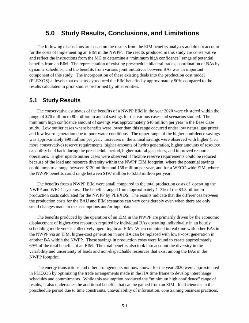
5.0 Study Results, Conclusions, and Limitations

The following discussions are based on the results from the EIM benefits analyses and do not account for the costs of implementing an EIM in the NWPP. The results produced in this study are conservative and reflect the instructions from the MC to determine a “minimum high confidence” range of potential benefits from an EIM. The representation of existing preschedule bilateral trades, coordination of BAs by dynamic schedules, and the benefits from various joint initiatives between BAs was an important component of this study. The incorporation of these existing deals into the production cost model (PLEXOS) at levels that exist today reduced the EIM benefits by approximately 50% compared to the results calculated in prior studies performed by other entities.

5.1 Study Results

The conservative estimates of the benefits of a NWPP EIM in the year 2020 were clustered within the range of $70 million to 80 million in annual savings for the various cases and scenarios studied. The minimum high confidence amount of savings was approximately $40 million per year in the Base Case study. Low outlier cases where benefits were lower than this range occurred under low natural gas prices and low hydro generation due to poor water conditions. The upper range of the higher confidence savings was approximately $90 million per year. Increases in the annual savings were observed with higher (i.e., more conservative) reserve requirements, higher amounts of hydro generation, higher amounts of resource capability held back during the preschedule period, higher natural gas prices, and improved resource operations. Higher upside outlier cases were observed if flexible reserve requirements could be reduced because of the load and resource diversity within the NWPP EIM footprint, where the potential savings could jump to a range between $130 million and 158 million per year, and for a WECC-wide EIM, where the NWPP benefits could range between $197 million to $233 million per year.

The benefits from a NWPP EIM were small compared to the total production costs of operating the NWPP and WECC systems. The benefits ranged from approximately 1–3% of the $3.3 billion in production costs calculated for the NWPP by PLEXOS. The results indicate that the differences between the production costs for the BAU and EIM scenarios can vary considerably even when there are only small changes made to the assumptions and/or input data.

The benefits produced by the operation of an EIM in the NWPP are primarily driven by the economic displacement of higher-cost resources required by individual BAs operating individually in an hourly scheduling mode versus collectively operating in an EIM. When combined in real time with other BAs in the NWPP via an EIM, higher-cost generation in one BA can be replaced with lower-cost generation in another BA within the NWPP. These savings in production costs were found to create approximately 69% of the total benefits of an EIM. The total benefits also took into account the diversity in the variability and uncertainty of loads and non-dispatchable resources that exist among the BAs in the NWPP footprint.

The energy transactions and other arrangements not now known for the year 2020 were approximated in PLEXOS by optimizing the trade arrangements made in the HA time frame to develop interchange schedules and commitments. While this assumption produced the “minimum high confidence” range of results, it also understates the additional benefits that can be gained from an EIM. Inefficiencies in the preschedule period due to time constraints, unavailability of information, constraining business practices,

5.1

and/or overly conservative margins to cover variability and load forecasting errors will be removed in an EIM. These benefits are in addition to capturing the benefits from more load and resource diversity and more efficient economic dispatch of the combination of resource stacks. Sensitivity cases were performed with energy and capacity held out of the preschedule interchanges and efficiency optimization. The results for these cases indicated significantly larger benefits for the EIM scenario than operation under the BAU scenario.

There is still substantial room for improvement in modeling hydro generation for energy constrained systems such as those in the NWPP. Excess hydro generation was used by PLEXOS when hydro generation could not be shaped properly over some periods. This excess hydro generation should have been replaced by the committed thermal generation that was available. To more accurately compare the production costs of the cases in this event, the Analytical Team developed an approach external to PLEXOS that values this additional excess hydro generation at the cost of available thermal generation in the surrounding time segments. This excess hydro generation was valued at two different price levels to provide a range of values for comparative purposes. The results from these valuations were included in the computations of total savings. A sensitivity case was also modeled using a “look ahead” technique where operators and dispatchers were assumed to have better ability to look ahead in the hour and adjust operations (as is done in real life). This approach yielded significant reductions in the amounts of excess hydro generation and significantly higher savings in production costs for the BAU scenario and EIM scenario with the total savings from an EIM increasing relative to the BAU.

Most of the cases were performed holding the same levels of capacity reserves going into the real time period in both the EIM and BAU scenarios since this was not a study of either the capacity savings which might accrue to an EIM or a resource sufficiency study. However, one such case was performed which indicated that the capacity reserve requirements could be reduced by approximately 30% with there being a substantial increase in savings for the EIM scenario compared to BAU scenario, if the BAs in the NW operated as a combined NWPP BA. The annual total savings in the range of $130 million to $160 million for this case was caused by fewer thermal units needing to be committed and, in turn, running at minimum generation levels. That also resulted in reducing NWPP EIM total annual export energy by 3.9% in comparison with the Base Case BAU scenario.

Several sensitivity cases examined the effect of increasing the amounts of capacity reserves to cover tail event variations by increasing the confidence interval for computing the amount of load following reserves. As expected, the higher amounts of capacity reserves held out to cover tail event variations in the individual BAs in the BAU scenarios caused an increase in the total savings from the operations of an EIM where the operations for the BAs are combined.

A sensitivity case was performed to determine the benefits of a WECC-wide EIM compared with a BAU scenario having WECC-wide hourly scheduling. The results for this sensitivity case indicate that under a WECC-wide EIM the NWPP would provide significant balancing and economic resource displacement benefits to California and overall WECC-wide societal benefits. The value of these benefits for the NWPP could be as high as $256 million per year.

A sensitivity case was also performed to quantify the effect of a NWPP EIM that is hypothetically without PacifiCorp being a member. The results from this case indicate that the EIM benefits to the remaining NWPP members would be reduced by approximately 10%.

5.2

Overall societal benefits for a NWPP EIM were also parsed and estimated for each of the individual BAs in the NWPP EIM footprint. Because of the large volumes of wind and hydro generation having zero marginal costs in the NWPP system, the use of locational imbalance prices was problematic and parsing was performed using the volume of transactions each BA made in the year 2020 based on the results from PLEXOS. The volumes of transactions reflected the differences in the amounts of sales or purchases each utility made in the EIM scenario compared to the BAU scenario. The parsing methodology measured the volumes of intra-hour transactions between the BAs and then assumed that the proportion of total annual savings would flow to the BAs in proportion to their respective shares of the overall transaction volume.

This parsing methodology was found to produce results that are stable and robust. The percentages of the parsed benefits for each individual BA in the NWPP EIM footprint were similar for most of the cases. It is expected that the relative differences between the cost of power purchases and revenue from surplus sales in the NWPP EIM will remain approximately the same between the BAs in the NWPP EIM footprint even if there are fluctuations in the market prices.

An analysis of the amounts of loadings on the major transmission paths (flowgates) in the WECC indicates that some flowgates become heavily loaded slightly more often in the EIM scenario than in the BAU scenario. However, there are also some flowgates which experience reductions in flows. The EIM scenarios were performed based on using a security constrained dispatch algorithm, which with a few exceptions where flow limits are violated in the simulations during the real time period, holds flowgate loadings below their system operating limits.

5.2 Limitations of Production Cost Modeling

The production cost model (PLEXOS) used by the MC Initiative Analytical Team produced results that are a rough surrogate for the results that would be obtained by modeling an EIM. PLEXOS was not designed to simulate the operation of a market, but rather the operation of a set of power system elements. Particularly challenging in the process was representing the complex monthly, weekly, hourly and intra-hour “budgeting” process for flexible hydroelectric facilities, which involves considering not just the immediate market value of the generation and unit capabilities, but also how operational and economic decisions made in one time frame might affect operational capabilities and economic conditions in future time frames.

This complexity resulted in PLEXOS not being able to accurately simulate a reasonable dispatch of significant amounts of hydroelectric resources within the NWPP for some outcomes. The Analytical Team had to develop an approach external to PLEXOS to address such outcomes. The way actual hydroelectric production decisions are made could have fairly significant effects on the modeling of hydro operations in and results from the PCM. Better modeling of the hydro generation for the energy constrained hydro systems that exist in the NW is needed.

The modeling effort used an Interchange Scheduling Method to more accurately represent the operation of individual BAs, which are responsible for balancing their own respective load and resource variability and forecast errors. Implementing this approach requires knowledge of contractual and other transactional arrangements between BAs. When these were specifically known and expected to remain in 2020, they were explicitly represented as best they could be modeled in PLEXOS. It is critical in an EIM

5.3

analysis to try and model preschedule efficiencies well. Any inefficiencies that remain in the HA periods will be removed and the benefits attributed to the EIM.

The instructions to the Analytical Team were to find the “minimum high confidence range of benefits” and also fix the four data issues discussed in Section 3.7. For these reasons, the interchange schedules between the BAs in the BAU scenarios were set based on results from the optimization of the HA period across the WECC with the exception of the known arrangements. Accordingly, the lack of information about known contracts and arrangements is a limitation of the modeling.

Despite these challenges, the expert economic dispatch analysts who participated in the Analytical Team have expressed a reasonable level of confidence in the results while acknowledging the complexities of the modeling process.

5.3 Suggested Improvements for Additional Analyses

If additional studies are required for either the NWPP MC Initiative or for other analyses relative to the work performed for the MC, there are many improvements that could be made to the information and logic of the PCM. Some of these improvements are the following:

• reviewing and scrubbing of data in the WECC-wide EIM case for other areas to the extent done by members of the NWPP for the NW area

• inputting better heat rate curves for thermal units

• better operational models of energy constrained coordinated hydro systems

• more detail on Canadian hydro and system operations

• faster and better ability to perform round trips between the power flow and voltage stability programs and the production cost model. This would allow reliability analyses to be performed.

• addition of market bidding algorithms, which could replicate voluntary bidding processes into the solution

• better understanding of the implications of 15-minute scheduling for an EIM.

Lastly, a WECC-wide home for the operational simulation data base is needed so that entities located throughout the WECC interconnection can use the data base and make improvements. This availability will allow joint studies by various entities within the WECC.

5.4

6.0 References

[1] Damiano P. 2013. The Northwest Power Pool Members’ Market Assessment and Coordination Committee (MC) Initiative – EMT WG & EIM WG Update. [Online.] Accessed August 15, 2013, at http://www.nwpp.org/documents/MC-Public/Jan.-25-Public-Meeting_NWPP-MC-EIM-EMT-Workgroup-Update.pdf.

[2] Western Electricity Coordinating Council. 2010. Assumptions Matrix for the 2020 TEPPC Dataset. [Online.] Accessed August 15, 2013, at http://www.wecc.biz/library/StudyReport/Documents/Assumptions%20Matrix%20for%20the%202020%20TEPPC%20Dataset.pdf.

[3] Orans R, A Olson and J Moore (E3: Energy and Environmental Economics). 2011. WECC EDT Phase 2 EIM Benefits Analysis & Results (October 2011 Revision). [Online.] Accessed August 15, 2013, at http://www.wecc.biz/committees/EDT/Documents/E3_EIM_Benefits_Study-Phase_2_Report_RevisedOct2011_CLEAN2[1].pdf.

[4] Samaan N, M Milligan, YV Makarov, M Hunsaker, T Nguyen, C Jin, R Diao and R Hafen. Balancing Authority Cooperation Concepts to Reduce Variable Generation Integration Costs in the Western Interconnection: Balancing Authorities Consolidation and Sharing of Balancing Reserves. Final Project Report, Pacific Northwest National Laboratory, Richland, Washington. To be published in November 2013.

[5] Hunsaker M, N Samaan, M Milligan, T Guo, G Liu and J Toolson. 2013. Balancing Authority Cooperation Concepts to Reduce Variable Generation Integration Costs in the Western Interconnection: Intra-Hour Scheduling. Final WECC Project Report. [Online.] Accessed August 15, 2013, at http://www.wecc.biz/committees/StandingCommittees/JGC/VGS/Shared%20Documents/BA%20Cooperation%20Study/Final%20Report/Balancing%20Authority%20Cooperation%20Concepts%20-%20Intra-Hour%20Scheduling.pdf.

[6] Milligan M, K Clark, J King, B Kirby, T Guo and G Liu. 2013. Examination of Potential Benefits of an Energy Imbalance Market in the Western Interconnection. NREL/TP-5500-57115. National Renewable Energy Laboratory, Golden, CO. [Online.] Accessed August 15, 2013, at http://www.nrel.gov/docs/fy13osti/57115.pdf.

[7] Nickell BM. 2008. TEPPC Renewable Energy Cases. [Online.] Accessed August 15, 2013, at http://www.wecc.biz/committees/StandingCommittees/PCC/LRS/Shared%20Documents/Wind%20Profiles/Renewable%20Energy%20Generation%20Paper.pdf.

[8] E3 – Energy and Environmental Economics. 2013. PacifiCorp-ISO Energy Imbalance Market Benefits. March 2013. [Online.] Accessed August 15, 2013, at http://www.caiso.com/Documents/PacifiCorp-ISOEnergyImbalanceMarketBenefits.pdf.

[9] 3TIER. 2010. Development of Regional Wind Resource and Wind Plant Output Datasets. NREL/SR-550-47676. Work performed by 3TIER for National Renewable Energy Laboratory,

6.1

Golden, CO. [Online.] Accessed August 15, 2013, at http://www.nrel.gov/docs/fy10osti/47676.pdf.

[10] Orwig K, M Hummon, BM Hodge and D Lew. 2011. Solar Data Inputs for Integration and Transmission Planning Studies. NREL/PO-5500-52985. National Renewable Energy Laboratory, Golden, CO.

[11] Ma J, YV Makarov, C Loutan, and Z Xie. 2011. “Impact of wind and solar generation on the California ISO’s intra-hour balancing needs.” IEEE 2011 Power and Energy Society General Meeting, pp.1-6, 24–29, July 2011. DOI: 10.1109/PES.2011.6039410.

[12] Makarov YV, C Loutan, J Ma, and P de Mello. 2009. “Operational Impacts of Wind Generation on California Power Systems.” IEEE Transactions on Power Systems 24(2):1039–1050. DOI: 10.1109/TPWRS.2009.2016364.

[13] “1997 Agreement for the hourly coordination of the projects on the Mid-Columbia river’, [Online.] Accessed August 15, 2013, at http://www.chelanpud.org/documents/MCHC_Agreement_97.pdf

6.2

Appendix A

Wind Crosswalk Data

Appendix A

Wind Crosswalk Data

Section 2.4 gave an overview of total installed capacity for each Balancing Authority (BA) in the Northwest Power Pool (NWPP). Appendix A provides more information about the wind power plants in the model in terms of the BA ownership, the bus the plant is connected to in the model, installed capacity, if they represent a wind power plant that is currently in service.

BA-Bus # Project Name Installed Capacity (MW) BA Total

AVA_wind_ 48383 Palouse Wind 105

AVA Total

105

BCTC_wind_50360

150 BCTC_wind_50364

334

BCTC_wind_50455

34 BCTC_wind_50559

504

BCTC_wind_50562

180 BCTC_wind_50653

180

BCTC Total

1381

BPA_wind_40111 BIG EDDY 313

BPA_wind_40125 Willow wind w1 72 BPA_wind_40477 LINDEN RANCH W1 231 BPA_wind_40666 RpsORwindWA1 590 BPA_wind_40671 LONGVIEW 89 BPA_wind_40686 SPRING CREEK 313 BPA_wind_40687 MALIN 332 BPA_wind_40723 RpsWAwnd3 547 BPA_wind_40913 SACAJAWEA 313 BPA_wind_41341 KLONDIKE 2 76 BPA_wind_41363 CONWIND_1 50 BPA_wind_41402 BIG HORN W2 511 BPA_wind_42063 LOWER SNAKE RVR 343 BPA_wind_47315 9CWIND 1_1 27 BPA_wind_47316 9CWIND 2_1 202 BPA_wind_47326 KLOND W1_1 25 BPA_wind_47327 HAY CANYON W1 746 BPA_wind_47452 SHEPHERDS FLAT W2 555 BPA_wind_47458 SHEPHERDS FLAT W3 290 BPA_wind_47573 STATL W1 1 90

A.1

BPA_wind_47801 HOPKR 1 300 BPA_wind_47802 HOPKR 2 157 BPA_wind_47814 PEBBLE SPRINGS W 100 BPA_wind_47827 HARVEST WIND 1 163 BPA_wind_47906 WHTCK W1 552 BPA_wind_47975 STAR POINT W1 100

BPA Total

7089 BPA Existing

4590

BPA RPS Future

2499

NWMT_wind_62036

188 NWMT_wind_62071 40 MW & 210 MW Glacier wind 250 NWMT_wind_62351

40

NWMT Total

478

PACE_ID_wind_65675

125

PACE_ID_wind_65680

164.5 PACE_UT_wind_66400

19

PACE_UT_wind_67826

86 PACE_WY_wind_65300

338

PACE_WY_wind_65420

424.5 PACE_WY_wind_65580

168.5

PACE_WY_wind_65584

52 PACE_WY_wind_65585

52

PACE_WY_wind_65778

284 PACE_WY_wind_67795

400

PACW_wind_44885 LEANING JUNIPER W1 100 PACW_wind_45233 ECHO WIND_1 64

PACW_wind_45566 COMBINE HILLS w1 41 PACW_wind_47816 LEANING JUNIPER W2 100 PACW_wind_47830 RPSCAWINDWA1 313 PAC_wind_47829 GOODNOE HILLS 94 PAC_wind_47571 STATL W2 1 210 PAC_wind_47550 VANSYCLE_1 124 PAC_wind_48221 MARENGO_2 227

PAC_wind_48451 MARENGO 227 PAC Total

3613.4

PGN_wind_47844 GOLDEN HILLS W1 106

PGN_wind_43950 RpsORwnd1 360 PGN_wind_43954 RpsCAwindOR1 404 PGN Total

870

A.2

PSE_wind_42364 WILDH 1 229 PSE_wind_42365 WILD HORSE 316 PSE Total

545

TREAS VLY_wind_60306

105 TREAS VLY_wind_60394

140

FAR EAST_wind_60062

125 MAGIC VLY_wind_60360

190

MAGIC VLY_wind_60395

140 MAGIC VLY_wind_61810

100

IPC Total

800

A.3

Appendix B

PNNL Flex Reserve Calculation Approach

Appendix B

PNNL Flex Reserve Calculation Approach

In this appendix, the methodology we developed to simulate essential balancing functions of a BA is explained. Actual scheduled net interchange, and 1-minute resolution load and wind data along with simulated real-time and hour-ahead forecast errors are used to obtain hour-ahead generation schedules, and load-following and regulation requirement curves. These curves are then analyzed for various metrics to evaluate the flex reserve requirements.

B.1 Simulation of the Hour-Ahead Schedules for Load and Wind Generation

The curves representing the hour-ahead schedules for load and wind generation are obtained from actual data as follows:

a. Use the actual 1-minute resolution “m” load data Lactual(m) (see blue curve shown in Figure B.1): Lactual(h) = 1/60 ΣLactual(m) for each hour “h” in the year (see red curve shown in Figure B.1).

b. Simulate the hour-ahead forecast error e[L(h)] for each hour in the year. The forecast error is assumed to follow the truncated normal distribution (TND) with certain specified statistical characteristics.

c. Calculate the hour-ahead load schedule Lschedule(h) by subtracting the load forecast error, calculated in Step b, from the actual hourly average calculated in Step a. Also, incorporate a 20-minute-duration ramp into the transition from one hour schedule to the next hour schedule.

Lschedule(h) = Ramp20 min {Lactual(h) − e[L(h)]} (see green curve shown below in Figure B.1).

Figure B.1. Simulation of Hour-Ahead Schedule for Load

0 2 4 6 8 10 12 14 16 18 20 22 24

5600

5800

6000

6200

6400

6600

6800

7000

7200

Time in hours

Load

(MW

)

Acutal loadhouly load averagehourly schedule

B.1

d. We proceed along the same lines as we did for load (steps a–c) to obtain an HA schedule for wind generation. Use the actual 1-minute resolution “m” wind data Wactual(m) to calculate the hourly wind average Wactual(h):

Wactual(h) = 1/60 ΣWactual(m) for each hour in the year

e. Simulate the hour-ahead forecast error e[W(h)] for each hour “h” in the year. The forecast error is assumed to follow the TND with certain specified statistical characteristics.

f. Calculate the hour-ahead wind schedule Wschedule(h) by subtracting the wind forecast error, calculated in Step e, from the actual hourly average calculated in Step d. Also, reflect a 20-minute ramp in the transition from one hour schedule to the next hour schedule:

Wschedule(h) = Ramp20 min{Wactual(h) − e[W(h)]}

B.2 Simulation of the Real-Time Schedule for Load and Wind Generation

The real-time (10-minute ahead) schedules for load and wind are obtained from actual data as follows:

a. Use the actual 1-minute resolution “m” load data Lactual(m) (see blue curve shown in Figure B.2) to calculate the 10-minute (10m) load average Lactual(10m):

Lactual(10m) = 1/10 ΣLactual(m) for each 10-minute interval in the year (see green curve shown in Figure B.2).

b. Simulate the real-time forecast error e[L(10m )] for each 10-minute interval in the year. The forecast error is assumed to follow the TND with certain specified statistical characteristics.

c. Simulate the 10-minute-ahead real-time load schedule Lschedule(10m) by subtracting the load forecast error, calculated in Step b, from the actual 10-minute average calculated in Step a. Also simulate the 10-minute transition from one 10-minute schedule to the next 10-minute schedule (i.e., by connecting midpoints of the subsequent 10-minute schedules):

Lschedule(10m) = Ramp10 min{Lactual(10mi) - e[L(10m)]} (see the magenta curve shown in Figure B.2).

B.2

Figure B.2. Simulation of the Real-Time Schedule for Load

d. The real-time schedule for wind generation is calculated in a different manner from the load schedule. The actual 1-minute resolution “m” wind data Wactual(m) is used to calculate the real-time wind schedule Wschedule(m). In the absence of real-time forecast data, a strategy that is adopted for the California Independent System Operator (CAISO) and the Bonneville Power Administration (BPA) in our previous efforts will be used. The persistence model is used to simulate real-time wind forecast. It assumes that the real-time wind forecast equals the actual wind production observed 7.5 minutes before the beginning of a dispatch interval:

Wschedule(10m) = Wactual(m − 7.5) for each minute in the year

Examples of the calculated real-time and hour-ahead schedules for load and wind are shown in Figure B.3 and Figure B.4, respectively.

0 20 40 60 80 100 1205350

5400

5450

5500

5550

5600

5650

5700

Time in minutes

Load

(MW

)

Acutal load10-min load averageReal time schedule

B.3

Figure B.3. Hour-Ahead and Real-Time Schedules for Load

Figure B.4. Hour-Ahead and Real-Time Schedules for Wind (based on BPA wind forecast statistics)

0 2 4 6 8 10 12 14 16 18 20 22 24 700

800

900

1000

1100

1200

1300

1400

Time(h)

Real time schedule Hour-ahead schedule

B.4

B.3 Simulation of the Regulation and Load-Following Curves

We treat wind as “negative load.” By doing so, we define the notion of “net load” in the ensuing analysis.

a. The minute-by-minute “Actual_net_load(m)” is calculated by subtracting the minute-by-minute actual wind generation from the minute-by-minute actual load, and by adding the net interchange:

Actual_net_load(m) = Lactual(m) – Wactual(m) + Net_interchange(m),

where Net_interchange(m) = Ramp20 min{Net_interchange(h)} for all “m” within “h.” It is assumed to be an export.

b. The net load (which is the same as hourly generation schedule), henceforth referred to as “Hour-ahead_schedule(h),” is calculated by subtracting the wind hourly schedule from the load hourly schedule and adding net interchange (see red curve shown in Figure B.5):

Hour-ahead_schedule(h) = Lschedule(h) – Wschedule(h) + Ramp20 min{Net_interchange(h)}

c. The real-time net load schedule (or real-time generation schedule or 10-minute-ahead schedule), henceforth referred to as real-time schedule, is calculated by subtracting the wind real-time schedule from the load real-time schedule and adding net interchange (see blue curve shown below in Figure B.5):

Real-time_schedule(10m)=Lschedule(10m) – Wschedule(10m) + Ramp10 min{Net_interchange(h)}

Figure B.5. Real-Time and Hour-Ahead Schedules

0 2 4 6 8 10 12 14 16 18 20 22 24 3500

4000

4500

5000

5500

6000

6500

Time(h)

Real time schedule Hour ahead schedule

Capacity (MW)

B.5

B.3.1 Generation Hour-Ahead Schedule Curve

The generation of hour-ahead schedule curve represents the total amount of generation to be scheduled to serve the net load in the next operating hour.

Generation_hour-ahead_schedule(m) = Hour_ahead_schedule(h) = Lscedule(h) – Wschedule(h) + Ramp20 min{Net_interchange(h)}

B.3.2 Load-Following Curve

The minute-to-minute load-following curve represents the load-following requirements within the hour time frame as a result of hour-ahead forecast errors and 1 hour discretization of the hour-ahead schedule. It is calculated by subtracting the hour-ahead schedule from the real-time schedule:

Load_following_curve(m) = Real-time_schedule (10m) – Hour_ahead_schedule(h) = [Lschedule(10m) – Wschedule(10m) + Ramp20 min{Net_interchange (h)}] –

[Lschedule(h) – Wschedule(h) + Ramp20 min{Net_interchange (h)}]

Or, which is the same,

Load_following_curve(m) = [Lschedule(10m) – Wschedule(10m)] – [Lschedule(h) – Wschedule(h)]

Figure B.6 and Figure B.7 show the real-time and hour-ahead schedules for load and wind. The resulting load-following curve is shown in Figure B.8. The load-following curve is independent of the net interchange.

Figure B.6. Actual Load Lactual(m) and Real-Time Load Schedule Lschedule(m)

B.6

Figure B.7. Actual Wind Wactual(m) and Real-time Wind Schedule Wschedule(m)

Figure B.8. Calculated Load-Following Requirements

0 2 4 6 8 10 12 14 16 18 20 22 24 750

800

850

900

950

1000

1050

1100

1150

1200

Time(h)

Actual wind Real time schedule for wind

B.7

B.3.3 Regulation Curve

The minute-to-minute regulation curve represents the regulation requirements within the 1- to 10-minute time frame appearing as a result of real-time forecast errors and 10-minute discretization of the real-time schedule. It is calculated by subtracting the real-time schedule from the actual net load. In mathematical terms, regulation is defined as

Regulation_curve(m) = Actual_net_load(m) – Real-time_schedule(10m) = [Lactual(m) – Wactual(m) + Ramp20 min{Net_interchange(h)}] – [Lschedule(10m) – Wschedule(10m) + Ramp20 min{Net_interchange(h)}]

or

Regulation_curve(m) = [Lactual(m) – Wactual(m)] – [Lschedule(10m) – Wschedule(10m)]

With Lactual(m) and Lschedule(10m) plotted in Figure B.6, and Wactual(m) and Wschedule(m) plotted in Figure B.7, the regulation curve would be as illustrated in Figure B.9.

It can be seen from the above equation that the regulation curve does not depend on the hourly scheduled net interchange.

Figure B.9. Calculated Regulation Requirement

B.8

B.4 Calculation of Balancing Reserve Requirments a. Each minute in the load-following, or regulation curves is characterized by capacity requirements.

b. As is the case with any methodology that is based on random number generators, in this case generation of load forecast errors, we do not rely on a single realization of a forecast error time series; rather, the previous steps are repeated 20 times (Monte Carlo simulation) with a different set of time series forecast errors for each run.

c. System operators are not required to balance against each point along the generation requirement curve. Therefore, a certain percentage of points could be left not completely balanced, say, 5% of points that can be considered as statistical outliers, i.e., those below and above certain threshold requirements are not considered for further analysis. This elimination is performed independently for each month for each BA.

d. For each hour in a day within the month, the maximum incremental and decremented capacity requirements for each of the load following and regulation curves are calculated. This is achieved by comparing all the points within the selected Convidenace Interval (CI) within this hour for certain month. A sample of results is shown in Figure B.10.

Figure B.10. Example of Load Following Capacity Requirement for 24 Operating Hours for Certain Month

B.9

Appendix C

Allocation of MidC Hydro Plants to Balancing Areas

Appendix C

Allocation of MidC Hydro Plants to Balancing Areas

The capacity of the projects was assigned to the individual balancing areas to correspond to the contractual share of the projects. This was done by adjusting the capacity of the individual units and electrically connecting one or more of the units to the balancing areas in a manner that approximated the contractual share.

C.1 Wells Jan Feb Mar April May June July Aug Sept Oct Nov Dec

Max. 850 850 850 850 850 850 850 850 850 850 850 850 Min. 100 100 100 100 100 100 100 100 100 100 100 100

Average 357 336 312 422 423 452 407 337 239 246 267 325

Share PAC 6.59% PGE 19.39% PSE 29.89%

AVA 7.84% MidC 36.29%

Type

HTC 50% Fixed 50%

C.2 Rocky Reach Jan Feb Mar April May June July Aug Sept Oct Nov Dec

Max. 1253 1035 1035 1035 1253 1253 1253 1035 1035 1035 1253 1253 Min. 100 100 100 100 100 100 100 100 100 100 100 100

Ave. 519 480 445 657 648 736 569 488 332 344 392 470 Share

PGE 3% PSE 25%

AVA 3% MidC 69%

Type

HTC 50% Fixed 50%

C.1

C.3 Rock Island Jan Feb Mar April May June July Aug Sept Oct Nov Dec

Max. 576 524 524 524 576 576 576 524 524 524 576 576 Min. 100 100 100 100 100 100 100 100 100 100 100 100

Average 227 214 199 261 266 285 217 202 144 152 179 209

Share PGE 3% PSE 25%

AVA 3% MidC 69%

Type

HTC 50% Fixed 50%

C.4 Wanapum Jan Feb Mar April May June July Aug Sept Oct Nov Dec

Max. 870 870 870 870 870 870 870 870 870 870 870 870 Min. 100 100 100 100 100 100 100 100 100 100 100 100 Average 459 426 402 508 537 489 529 438 282 294 362 417 Share

PAC 1.55 PGE 9.06 PSE 0.89

AVA 3.98 BPA 13.81 SCL 0.39

TPWR 0.4 MidC 69.92

Type

HTC 50% Fixed 50%

C.2

C.5 Priest Rapids Jan Feb Mar April May June July Aug Sept Oct Nov Dec

Max. 880 880 880 880 880 880 880 880 880 880 880 880

Min. 200 200 200 200 200 200 200 200 200 200 200 200 Average 455 408 392 415 549 519 434 387 278 285 339 412 Share

PAC 1.6% PGE 9.1% PSE 0.9%

AVA 4.0% BPA 13.8% SCL 0.4% TCL 0.4%

MidC 69.9% Type

HTC 20% Fixed 80%

C.3

Appendix D

Remote Units Providing only Contingency Reserve

Appendix D

Remote Units Providing only Contingency Reserve

Unit Capacity

(MW) Owner Located In BA Owner in BA % Share

Cap. Share (MW)

Colstrip 1,2

Colstrip 1,2 614 NWMT NWMT NWMT 50.00% 307.0 Colstrip 1,2 614 PSE NWMT PSE 50.00% 307.0 Colstrip 3,4

Colstrip 3,4 1,480 AVA NWMT AVA 15.00% 222.0 Colstrip 3,4 1,480 NWMT NWMT NWMT 30.00% 444.0 Colstrip 3,4 1,480 PAC NWMT PACW 10.00% 148.0 Colstrip 3,4 1,480 PGN NWMT PGN 20.00% 296.0 Colstrip 3,4 1,480 PSE NWMT PSE 25.00% 370.0 Intermountain 1,2

Intermountain 1,2 1,920 ANHM LDWP CAISO 13.20% 253.4 Intermountain 1,2 1,920 BURB LDWP LDWP 3.40% 65.3 Intermountain 1,2 1,920 GLEN LDWP LDWP 1.70% 32.6 Intermountain 1,2 1,920 ICPA LDWP LDWP 21.10% 405.1 Intermountain 1,2 1,920 LDWP LDWP LDWP 44.60% 856.3 Intermountain 1,2 1,920 PAC LDWP PACE 4.00% 76.8 Intermountain 1,2 1,920 PASA LDWP CAISO 4.40% 84.5 Intermountain 1,2 1,920 RVSD LDWP CAISO 7.60% 145.9

Ownership by BA: LDWP 71% 1,359.4

CAISO 25% 483.8

PACE 4% 76.8

Four Corners 4,5

Four Corners 4,5 1,480 APS APS APS 0.15 222.0 Four Corners 4,5 1,480 EPE APS EPE 0.07 103.6 Four Corners 4,5 1,480 PNM APS PNM 0.13 192.4 Four Corners 4,5 1,480 APS APS APS 0.48 710.4 Four Corners 4,5 1,480 SRP APS SRP 0.10 148.0 Four Corners 4,5 1,480 TEP APS TEP 0.07 103.6

Ownership by BA: APS 0.63 932.4

EPE 0.07 103.6

PNM 0.13 192.4

SRP 0.10 148.0

TEP 0.07 103.6

D.1

Navajo 1-3

Navajo 1-3 2,250 APS SRP APS 0.14 315.0 Navajo 1-3 2,250 LDWP SRP LDWP 0.21 477.0 Navajo 1-3 2,250 NEVP SRP NEVP 0.11 254.3 Navajo 1-3 2,250 SRP SRP SRP 0.46 1,035.0 Navajo 1-3 2,250 TEP SRP TEP 0.08 168.8 Palo Verde 1-3

Palo Verde 1-3 4,050 APS APS APS 0.29 1,178.6 Palo Verde 1-3 4,050 AZSA APS CAISO 0.00 2.4 Palo Verde 1-3 4,050 BNNG APS CAISO 0.00 2.4 Palo Verde 1-3 4,050 BURB APS LDWP 0.00 10.5 Palo Verde 1-3 4,050 CLTN APS CAISO 0.00 2.4 Palo Verde 1-3 4,050 EPE APS EPE 0.16 639.9 Palo Verde 1-3 4,050 GLEN APS LDWP 0.00 10.5 Palo Verde 1-3 4,050 IID APS IID 0.00 15.4 Palo Verde 1-3 4,050 LDWP APS LDWP 0.10 391.2 Palo Verde 1-3 4,050 PASA APS CAISO 0.00 10.5 Palo Verde 1-3 4,050 PNM APS PNM 0.10 413.1 Palo Verde 1-3 4,050 RVSD APS CAISO 0.00 13.0 Palo Verde 1-3 4,050 SCE APS CAISO 0.16 639.9 Palo Verde 1-3 4,050 SRP APS SRP 0.17 708.3 Palo Verde 1-3 4,050 VERN APS CAISO 0.00 11.7

Ownership by BA: APS 0.29 1,178.6

CAISO 0.17 682.4

EPE 0.16 639.9

IID 0.00 15.4

LDWP 0.10 412.3

PNM 0.10 413.1

SRP 0.17 708.3

San Juan 1

San Juan 1 327 PNM PNM PNM 0.5000 163.5 San Juan 1 327 TEP PNM TEP 0.5000 163.5 San Juan 2

San Juan 2 316 PNM PNM PNM 0.5000 158.0 San Juan 2 316 TEP PNM TEP 0.5000 158.0 San Juan 3

San Juan 3 498 PNM PNM PNM 0.5000 249.0 San Juan 3 498 AZSA PNM CAISO 0.0615 30.6 San Juan 3 498 BNNG PNM CAISO 0.0410 20.4 San Juan 3 498 CLTN PNM CAISO 0.0615 30.6 San Juan 3 498 TSGT PNM WACM 0.0820 40.8 San Juan 3 498 GLEN PNM LDWP 0.0410 20.4

D.2

San Juan 3 498 IID PNM IID 0.2130 106.1

Ownership by BA: PNM 0.5000 249.0

CAISO 0.1640 81.7

WACM 0.0820 40.8

LDWP 0.0410 20.4

IID 0.2130 106.1

San Juan 4

San Juan 4 507 ANHM PNM CAISO 0.1004 50.9 San Juan 4 507 FARM PNM PNM 0.0843 42.7 San Juan 4 507 LAC PNM PNM 0.0723 36.7 San Juan 4 507 MSR PNM BANC 0.2871 145.6 San Juan 4 507 PNM PNM PNM 0.3849 195.1 San Juan 4 507 UAMP PNM CAISO 0.0709 35.9

Ownership by BA: PNM 0.5415 274.5

CAISO 0.1713 86.8

BANC 0.2871 145.6

Craig 1,2

Craig 1,2 820 PAC WACM PACW 0.1900 156 Craig 1,2 820 PRPA WACM WACM 0.1800 148 Craig 1,2 820 PSC WACM PSCO 0.1000 82 Craig 1,2 820 SRP WACM SRP 0.2900 238 Craig 1,2 820 TSGT WACM WACM 0.2400 197

Ownership by BA: PSCO 0.1000 82.0

WACM 0.4200 344.4

PACW 0.1900 155.8

SRP 0.2900 237.8 Hayden 1

Hayden 1 203 PAC WACM PACW 0.2450 50 Hayden 1 203 PSC WACM PSCO 0.7550 153 Hayden 2

Hayden 2 286 PAC WACM PACW 0.1260 36 Hayden 2 286 PSC WACM PSCO 0.3740 107 Hayden 2 286 SRP WACM SRP 0.5000 143 Laramie River 2,3

Laramie River 2,3 1107 BEPC WACM WACM 0.5918 655 Laramie River 2,3 1107 LAC WACM PNM 0.0091 10 Laramie River 2,3 1107 MEAN WACM WACM 0.0164 18

D.3

Laramie River 2,3 1107 TSGT WACM WACM 0.3618 401 Laramie River 2,3 1107 WMPA WACM WACM 0.0209 23

Ownership by BA: WACM 0.9909 1,096.9

PNM 0.0091 10.1 Wyodak 1

Wyodak 1 340 BHPL PACE WACM 0.2000 68 Wyodak 1 340 PACE PACE PAC 0.8000 272 Gianelli (San Luis)

Gianelli (San Luis) 362 DWR CAISO CAISO 0.5500 199 Gianelli (San Luis) 362 WAPA CAISO BANC 0.4500 163 Luna CC

Luna CC 575 PNM PNM PNM 0.6667 383.3 Luna CC 575 TEP PNM TEC 0.3333 191.7 Springerville 3

Springerville 3 400 TSGT TEP WACM 0.7500 300.0 Springerville 3 400 SRP TEP SRP 0.2500 100.0

D.4

Appendix E

Flows at Selected WECC Paths and BA-to-BA Flowgates

Appendix E

Flows at Selected WECC Paths and BA-to-BA Flowgates

The Pacific Northwest National Laboratory (PNNL) team has developed a Microsoft® Bing® map-based tool to help in comparing transmission flows at different time frames for different simulation cases. The tool can be used for both Western Electricity Coordinating Council (WECC) path flows and Balancing Authority (BA)-to-BA flows. The tool is made available for Northwest Power Pool (NWPP) members to perform further transmission analysis as needed in the future. Snapshots of the tool are shown in Figure E.1.

Figure E.1. Snapshots of the Bing Map-Based Visualization Tool Developed by PNNL

E.1

Figure E.2 to Figure E.6 show comparisons of selected WECC path flows in hour-ahead (HA), business-as-usual (BAU) and Energy Imbalance Market (EIM) simulations for Core Case 1.86A in comparison to actual flows in 2011. Actual flows are used as a relative comparison and for building confidence in modeled results.

Figure E.2. WECC Path 3 (Northwest-Canada) Flow Comparison

E.2

Figure E.3. WECC Path 8 (Montana - Northwest) Flow Comparison

E.3

Figure E.4. WECC Path 65 (Pacific DC Intertie) Flow Comparison

E.4

Figure E.5. WECC Path 66 (COI) Flow Comparison

E.5

Figure E.6. WECC Path 76 (Alturas Project) Flow Comparison

Figure E.7 to Figure E.12 give BA-to-BA flows for selected BA-to-BA flowgates in the model. Comparisons are between HA, BAU and EIM flow patterns; there was no actual BA-to-BA flow data available to the study team.

E.6

Figure E.7. BPA to BANC Transmission Flows

BPA-BANC Power Flow

BPA-BANC Power Flow

E.7

Figure E.8. BPA to CAISO Transmission Flows

E.8

Figure E.9. PACW to CAISO Transmission Flows

E.9

Figure E.10. IPC to PACW Transmission Flows

E.10

Figure E.11. IPC to PACE Transmission Flows

E.11

Figure E.12. AVA to BPA Transmission Flows

E.12

Appendix F

Reserve Shift Analysis: Impact of Half-Hour Wind Scheduling on Load-Following Requirements

Appendix F

Reserve Shift Analysis: Impact of Half-Hour Wind Scheduling on Load-Following Requirements Background

The objective of the analysis in this section is to capture the impact of half-hour wind scheduling (applied to several specified wind farms) within BAs that normally schedule their generation on the hourly basis. While the analysis in this section is not directly related to the EIM analyses that were given in previous chapters, it highlights the benefits of a short-term alternative.

The analysis was conducted for a limited number of specified BAs that are described as source (e.g., BPA) and sink (e.g., PGN) BAs. The main idea is that if the source BA could schedule interchange for wind on a half-hourly basis, it would make the schedule follow its net load more closely. The scheduling change in the source BA is matched by adding the corresponding component to the net load in the sink BA. The load-following requirements should be calculated: (a) by the difference between the net load and modified schedule in the source BA, and (b) by the difference between modified net load and unchanged hourly schedule in the sink BA. The schedules should be ramped over 20 minutes between hours and over 10 minutes on the half-hour transitions. The analysis uses the assumptions and models developed for the ongoing study conducted by NWPP and PNNL. NWPP has provided information about the sink and source BAs, as well as wind farms participating in the half-hour scheduling process. Results are presented as hourly upward and downward load-following requirements in the source and sink BAs and compared with the results of the Core Case Reserve method, where all generators are scheduled on the hourly basis.

F.1 Objectives

In this work, PNNL team modified its original algorithms to calculate load-following requirements for selected source/sink BAs in the NWPP and run simulations based on NWPP specifications. The input data, such as load and wind generation, remain the same as the data used in the current NWPP EIM study, i.e., the 11% renewable penetration case. The changes made in load-following calculation include:

a. Modify the calculation of load-following component between source BAs and sink BAs. The source BA is defined as the one that sends wind energy from a specified wind farm to a sink BA, and the sink BA is the one that receives wind energy from a source BA.

b. Change wind forecast from hourly schedule to 30-minute schedule for a number of selected wind farms in source BAs. The rest of the wind farms in the source BA should have hourly schedules as before. No change is made to the wind and load schedules for sink BAs (hourly schedule). A persistence model is used to generate wind forecasts.

c. Adjust wind ramps within the hour: use 20-minute ramps for between-hour schedules and 10-minute ramps for within-hour schedules.

F.1

F.2 Approach

In this section, we use the sample plots obtained from BPA as an example to demonstrate the methodologies to compute load-following requirements using the modified algorithms.

For Source BAs (e.g., BPA), the scheduling procedure is shown in Figure F.1.

a. The dashed blue curve is the net load schedule using an hourly scheduling method for load and wind, the black solid curve is the actual net load, and the dashed yellow line is the modified net load schedule considering 30-minute wind schedules. Interchange schedules are not considered.

b. For selected wind farms in the source BA, a new 30-minute schedule is created. At the beginning of the hour, the T − 31 persistence model is used to generate the first 30-minute schedule; for the second 30-minute schedule, the T − x model is used, where x is flexible. In this study, we assume x = 1.

c. For the load hourly schedules, PNNL’s forecast error generator was used with the parameters set exactly as in the current NWPP EIM study.

d. For the rest of the wind farms in the source BA, only hourly schedule is considered, using the T − 31 model.

e. Ramps are created in between-hour schedules (20-minute ramp) and within-hour schedules (10-minute ramp)

f. Load following = RT schedule of net load (10-minute average of net load curve)—modified net load schedules considering 30-minute schedules of selected wind farms. That is, the difference between the average of the black solid curve and the dashed yellow curve.

Figure F.1. Scheduling Procedure for Source BAs

For Sink BAs (e.g., PGN), the computation of the load-following component is dependent upon the change calculated in the source BA. The scheduling procedure in a sink BA is shown in Figure F.2.

a. In Figure F.2, the dashed blue curve is the original hourly schedule of net load, the solid yellow curve is the actual net load based on a modified 30-minute wind schedule in the source BA, and the solid blue curve is the net load in the original case without schedule modifications.

6800.0

7000.0

7200.0

7400.0

7600.0

7800.0

8000.0

8200.0

8400.0

8600.0

8800.0

17:50

17:55

18:00

18:05

18:10

18:15

18:20

18:25

18:30

18:35

18:40

18:45

18:50

18:55

19:00

19:05

19:10

19:15

19:20

19:25

19:30

19:35

19:40

19:45

19:50

19:55

20:00

20:05

BA ActualHourly Load + Half-Hourly Persistence Interchange ScheduleHourly Load + Hourly Persistence Interchange Schedule

F.2

b. For the net-load hourly schedules, PNNL’s forecast error generator was used with the parameters set exactly as in the current NWPP EIM study.

c. Let’s define DiffsourceBA as the difference between the modified 30-minute wind schedule and the original hourly wind schedule, which is the difference between the dashed yellow curve and the dashed blue curve shown in Figure F.1. Then, the modified net load in the sink BA (the solid yellow curve in Figure F.2) is obtained by subtracting DiffsourceBA from the original net load in the sink BA (the dashed blue curve in Figure F.2).

d. The load-following component in a sink BA is calculated as the difference between the 10-minute average of modified net load (the solid yellow curve), and the original hourly schedule of net load (the dashed blue curve).

e. In some scenarios, only a specified fraction of wind generation of selected wind farms in the source BA is shifted to the sink BA. In these instances, only the corresponding fraction of DiffsourceBA is subtracted from the sink BA net load.

The rest of the analysis was exactly the same as in the methods PNNL is using for the NWPP study, including forecast error generation, result reporting method (on an hourly basis), etc. Load-following requirements in the source and sink BAs will be compared against the same quantities in the original case.

Figure F.2. Scheduling Procedure for Sink BAs

The above method also works for the wind transfers between one source BA and multiple sink BAs. The load-following requirements of sink BAs are calculated independently. For the source BA, the aggregated impact of the half-hour wind schedule can be calculated by simply summing up all the 30-minute schedules of individual wind transfers to multiple sink BAs.

20000

20500

21000

21500

22000

22500

23000

23500

24000

24500

25000

1 2 3 4 5 6 7 8 9 10 11 12 13 14 15 16 17 18 19 20 21 22 23 24 25 26 27 28

Load less Hourly Persistence Wind Schedule Net Hourly Persistence Wind LoadNet Half-Hourly Persistence Wind Load

F.3

F.3 Case Study One: Biglow Canyon Wind Transfer from BPA to PGN

F.3.1 Wind Farm Data Generation

A wind farm, Biglow Canyon, with an installed capacity of 450 MW located in BPA is used as an example to show the impact of half-hour wind schedule on the load-following requirements of both source and sink BAs. This wind transfer is currently being deployed in BPA, to transfer wind energy to PGN. To generate the wind power output of this wind farm, the NREL per-unit wind production profile at each bus is used. This wind farm is connected to three buses, 47906, 47327 and 40477, with capacities of 126 MW, 149 MW and 175 MW, respectively. The output of this wind farm (shown in Figure F.3) is the sum of the individual outputs at these three buses, which are calculated using the bus-level per-unit profile multiplied by its installed capacity.

Figure F.3. Power Output of Biglow Canyon in 2020

March June September0

50

100

150

200

250

300

350

400

450

Bigl

ow C

anyo

n W

ind

Farm

Pow

er O

utpu

t in

2020

MW

F.4

F.3.2 Example of Hourly Load Schedule

Figure F.4 shows the actual load in BPA and the generated hourly load schedule, with 20-minute ramps.

Figure F.4. Load and Hourly Load Schedule in BPA, January 2020

F.3.3 Example of 30-Minute Wind Schedule for Selected Wind Farms

Figure F.5 shows the actual wind production (blue curve), the generated hourly schedule with 20-minute ramps using the T − 31 persistence model (dashed green curve) and the generated 30-minute schedule with ramps using the modified algorithm (red curve). It clearly shows that the 30-minute wind schedule is closer to the actual wind output, compared to the hourly schedule, which provides a lower forecast error.

1.15 1.2 1.25 1.3 1.35 1.4 1.45x 104

6000

6500

7000

7500

8000

8500

9000

9500

time in minutes

Load

vs

hour

ly fo

reca

st (s

ched

ule)

, MW

actual loadhourly schedule

20-min ramps

F.5

Figure F.5. 30-Minute Wind Schedules for Biglow Canyon, January 2020

Figure F.6 shows the difference between the 30-minute wind schedule and the hourly schedule in the source BA. This time series was used to modify the net load curve in the corresponding sink BA and calculate its load-following requirements. Figure F.7 plots the difference between actual wind output and 30-minute schedule for Biglow Canyon.

Figure F.6. Difference between 30-Minute Wind Schedule of Biglow Canyon and the Hourly Schedule,

January 2020

1.9 1.95 2 2.05 2.1x 104

50

100

150

200

250

300

350

400

time in minutes

MW

Actual wind, 30-min wind schedule and hourly wind schedule

actual wind30-min schedule w/ rampshourly schedule w/ ramps

hourly forecast w/ 20min ramps

30-min forecast w/ 20min and 10min ramps

0 0.5 1 1.5 2 2.5 3 3.5 4 4.5x 104

-100

-50

0

50

100

150

time in minutes

Diff

eren

ce b

etw

een

30-m

in s

ched

ule

and

hour

ly s

ched

ule,

MW

F.6

Figure F.7. Difference between Actual Wind Output and 30-Minute Schedule, January 2020

F.3.4 Impact on BPA Load Following with 95% Confidence Level

This section shows the impact of a 30-minute wind schedule on BPA load-following requirements, calculated using a 95% CL. The study was conducted for the 12 months in the study year 2020. In this report, only the study results for three representative months are shown: January, April and August. The results for the other months are available upon request.

F.3.4.1 January 2020

Figure F.8. Impact on BPA Load Following, 95% CL, January 2020

0 0.5 1 1.5 2 2.5 3 3.5 4 4.5x 104

-250

-200

-150

-100

-50

0

50

100

150

200

Time in minutes, January 2020

Diff

eren

ce b

etw

een

actu

al w

ind

and

30-m

in s

ched

ule,

MW

1 2 3 4 5 6 7 8 9 10 11 12 13 14 15 16 17 18 19 20 21 22 23 240

500

1000

Operating Hour

Load

follo

win

g up

MW

Average change, -12.39 MW for ramping up and 10.77 MW for ramping down

hourly schedule30min schedule

1 2 3 4 5 6 7 8 9 10 11 12 13 14 15 16 17 18 19 20 21 22 23 24-1200

-1000

-800

-600

-400

-200

0

Operating Hour

Load

follo

win

g do

wn

MW

F.7

Table F.1. Difference between 30-Minute Schedule and Hourly Schedule in Figure F.8 (MW)

Operating Hour 1 2 3 4 5 6 7 8 9 1 0 1 1 12 13 1 4 1 5 16 17 18 1 9 20 2 1 2 2 2 3 2 4

Difference, up -1 1 -1 0 -1 5 -4 1 2 -1 9 -1 4 -2 7 -4 9 -8 -1 -4 0 -1 4 -6 -3 -1 2 -1 9 -1 7 -5 -2 1 -5 1 -3 -8

Difference, down 23 7 22 2 1 1 -1 13 -2 13 8 0 0 7 1 1 8 26 6 6 1 7 21 3 2 1 7 7 -5

Due to the modified 30-minute wind schedule of Biglow Canyon, the load-following requirement of BPA is decreased by 12.39 MW for ramping up (Inc) and decreased by 10.77 MW for ramping down (Dec), on average. It is important to note that a negative sign is used in this study for ramping down requirements, therefore a positive change (e.g., the second row of Table F.1) indicates a decreased amount of load-following requirement, and vice versa.

F.3.4.2 April 2020

Figure F.9. Impact on BPA Load Following, 95% CL, April 2020

Table F.2. Difference Between 30-Minute Schedule and Hourly Schedule in Figure F.9 (MW)

Operating Hour 1 2 3 4 5 6 7 8 9 1 0 11 1 2 13 1 4 15 1 6 1 7 1 8 1 9 20 2 1 22 2 3 24

Difference, up 1 -18 -30 -13 -3 -12 2 -2 -28 -3 -13 5 -16 -2 -11 -1 -4 -9 -9 -19 -1 -19 1 -11

Difference, down 12 -1 1 7 1 46 3 10 4 0 5 4 13 9 7 4 7 47 11 18 14 39 12 6

The load-following requirement is decreased by 8.96 MW for ramping up (Inc) and decreased by 11.65 MW for ramping down (Dec), on average.

1 2 3 4 5 6 7 8 9 10 11 12 13 14 15 16 17 18 19 20 21 22 23 240

200

400

600

800

1000

Operating Hour

Load

follo

win

g up

, MW

Average change, -8.96 MW for ramping up and 11.65 MW for ramping down

hourly schedule30min schedule

1 2 3 4 5 6 7 8 9 10 11 12 13 14 15 16 17 18 19 20 21 22 23 24-1500

-1000

-500

0

Operating Hour

Load

follo

win

g do

wn,

MW

F.8

F.3.4.3 August 2020

Figure F.10. Impact on BPA Load Following, 95% CL, August 2020

Table F.3. Difference between 30-Minute Schedule and Hourly Schedule in Figure F.10 (MW)

Operating Hour 1 2 3 4 5 6 7 8 9 10 11 12 13 14 15 16 17 18 19 20 21 22 23 24

Difference, up - 3 - 7 -12 -17 - 9 -16 -19 -20 - 8 -1 -7 -20 -35 -3 -2 -2 -5 -3 -3 -7 -15 0 -5 -12

Difference, down 9 0 9 7 1 5 4 0 6 10 18 3 2 -5 2 6 20 5 19 58 17 16 -8 2

The load-following requirement is decreased by 9.6 MW for ramping up (Inc) and decreased by 8.48 MW for ramping down (Dec), on average.

F.3.5 Impact on BPA Load Following with 99.5% Confidence Level

This section shows the impact of the modified wind schedule on load-following requirements of BPA with a higher CL, 99.5%.

1 2 3 4 5 6 7 8 9 10 11 12 13 14 15 16 17 18 19 20 21 22 23 240

200

400

600

800

1000

Operating Hour

Load

follo

win

g up

, MW

Average change, -9.6 MW for ramping up and 8.48 MW for ramping down

hourly schedule30min schedule

1 2 3 4 5 6 7 8 9 10 11 12 13 14 15 16 17 18 19 20 21 22 23 24-2000

-1500

-1000

-500

0

Operating Hour

Load

follo

win

g do

wn,

MW

F.9

F.3.5.1 January 2020

Figure F.11. Impact on BPA Load Following, 99.5% CL, January 2020

Table F.4. Difference between 30-Minute Schedule and Hourly Schedule in Figure F.11 (MW)

Operating Hour 1 2 3 4 5 6 7 8 9 10 11 12 13 14 15 16 17 1 8 1 9 20 2 1 2 2 23 24

Difference, up -47 2 -5 -7 -30 -30 -30 -38 -9 -18 -25 -45 -21 -17 -14 -23 -33 -4 -1 -40 -6 0 -25 -12

Difference, down 79 7 1 5 123 6 0 13 12 4 14 - 5 57 34 0 17 - 2 16 2 2 1 29 4 3 2 16 14

The load-following requirement is decreased by 19.92 MW for ramping up (Inc) and decreased by 21.55 MW for ramping down (Dec), on average.

1 2 3 4 5 6 7 8 9 10 11 12 13 14 15 16 17 18 19 20 21 22 23 240

500

1000

1500

2000

Operating Hour

Load

follo

win

g up

, MW

Average change, -19.92 MW for ramping up and 21.55 MW for ramping down

hourly schedule30min schedule

1 2 3 4 5 6 7 8 9 10 11 12 13 14 15 16 17 18 19 20 21 22 23 24-2000

-1500

-1000

-500

0

Operating Hour

Load

follo

win

g do

wn,

MW

F.10

F.3.5.2 April 2020

Figure F.12. Impact on BPA Load Following, 99.5% CL, April 2020

Table F.5. Difference between 30-Minute Schedule and Hourly Schedule in Figure F.12 (MW)

Operating Hour 1 2 3 4 5 6 7 8 9 10 11 12 13 14 15 16 17 18 19 20 21 22 23 24

Difference, up 1 -25 -49 -43 0 -28 -16 -9 -13 -27 -34 -1 -15 -6 -6 -8 -15 0 -14 -29 -4 -9 5 7

Difference, down 50 -5 2 11 9 1 3 12 10 -8 60 19 13 24 7 6 9 43 1 38 4 31 24 6

The load-following requirement is decreased by 14.06 MW for ramping up (Inc) and decreased by 15.47 MW for ramping down (Dec), on average.

1 2 3 4 5 6 7 8 9 10 11 12 13 14 15 16 17 18 19 20 21 22 23 240

500

1000

1500

Operating Hour

Load

follo

win

g up

, MW

Average change, -14.06 MW for ramping up and 15.47 for ramping down

hourly schedule30min schedule

1 2 3 4 5 6 7 8 9 10 11 12 13 14 15 16 17 18 19 20 21 22 23 24-2000

-1500

-1000

-500

0

Operating Hour

Load

follo

win

g do

wn,

MW

F.11

F.3.5.3 August 2020

Figure F.13. Impact on BPA Load Following, 99.5% CL, August 2020

Table F.6. Difference between 30-Minute Schedule and Hourly Schedule in Figure F.13 (MW)

Operating Hour 1 2 3 4 5 6 7 8 9 10 11 12 13 14 15 16 17 18 19 20 21 22 23 24

Difference, up -3 -10 -43 -23 -3 -14 -17 -18 -7 -1 -17 -42 -34 -40 -8 -3 -5 0 -4 -6 0 0 -1 -14

Difference, down 12 35 - 4 8 10 2 0 0 10 5 0 26 7 -1 1 16 39 12 64 20 74 6 -20 21

The load-following requirement is decreased by 13.11 MW for ramping up (Inc) and decreased by 14.31 MW for ramping down (Dec), on average.

F.3.6 Impact on PGN Load Following with 95% Confidence Level

This section shows the impact of the modified wind schedule on load-following requirements in PGN, with a CL of 95%.

1 2 3 4 5 6 7 8 9 10 11 12 13 14 15 16 17 18 19 20 21 22 23 240

500

1000

1500

Operating Hour

Load

follo

win

g up

, MW

Average change, -13.11 MW for ramping up and 14.31 MW for ramping down

1 2 3 4 5 6 7 8 9 10 11 12 13 14 15 16 17 18 19 20 21 22 23 24-3000

-2000

-1000

0

Operating Hour

Load

follo

win

g do

wn,

MW

hourly schedule30min schedule

F.12

F.3.6.1 January 2020

Figure F.14. Impact on PGN Load Following, 95% CL, January 2020

Table F.7. Difference between 30-Minute Schedule and Hourly Schedule in Figure F.14 (MW)

Operating Hour 1 2 3 4 5 6 7 8 9 10 11 12 13 14 15 1 6 17 1 8 19 20 21 22 2 3 24

Difference, up -11 6 -6 -4 1 5 2 10 5 21 15 6 0 3 -1 1 1 8 7 5 7 6 0 7 -3

Difference, down -25 -19 -23 -17 -1 0 0 0 -9 23 0 -4 7 -2 -8 -12 -8 -11 -8 -9 -9 -4 -15 4

The load-following requirement is increased by 4.08 MW for ramping up (Inc) and increased by 6.34 MW for ramping down (Dec), on average.

1 2 3 4 5 6 7 8 9 10 11 12 13 14 15 16 17 18 19 20 21 22 23 240

100

200

300

400

Operating Hour

Load

follo

win

g up

, MW

Average change, 4.08 MW for ramping up and -6.34 MW for ramping down

hourly schedule30min schedule

1 2 3 4 5 6 7 8 9 10 11 12 13 14 15 16 17 18 19 20 21 22 23 24-400

-300

-200

-100

0

Operating Hour

Load

follo

win

g do

wn,

MW

F.13

F.3.6.2 April 2020

Figure F.15. Impact on PGN Load Following, 95% CL, April 2020

Table F.8. Difference between 30-Minute Schedule and Hourly Schedule in Figure F.15 (MW)

Operating Hour 1 2 3 4 5 6 7 8 9 10 11 12 13 14 15 16 17 18 19 20 21 22 23 24

Difference, up -3 20 13 0 6 4 -44 -1 15 0 -17 -19 5 1 1 9 5 -19 -6 31 -13 -3 -3 10

Difference, down -1 6 1 39 1 2 0 3 5 0 -9 -5 -4 -12 -6 -2 6 -25 1 -9 6 1 -4 9

The load-following requirement is decreased by 0.38 MW for ramping up (Inc) and decreased by 0.05 MW for ramping down (Dec), on average.

1 2 3 4 5 6 7 8 9 10 11 12 13 14 15 16 17 18 19 20 21 22 23 240

100

200

300

400

Operating Hour

Load

follo

win

g up

, MW

Average change, -0.38 MW for ramping up and 0.05 MW for ramping down

1 2 3 4 5 6 7 8 9 10 11 12 13 14 15 16 17 18 19 20 21 22 23 24-400

-300

-200

-100

0

Operating Hour

Load

follo

win

g do

wn,

MW

hourly schedule30min schedule

F.14

F.3.6.3 August 2020

Figure F.16. Impact on PGN Load Following, 95% CL, August 2020

Table F.9. Difference between 30-Minute Schedule and Hourly Schedule in Figure F.16 (MW)

Operating Hour 1 2 3 4 5 6 7 8 9 1 0 1 1 1 2 1 3 1 4 1 5 1 6 17 18 19 2 0 2 1 2 2 2 3 2 4

Difference, up 8 5 2 5 8 1 1 1 2 1 4 9 2 1 7 2 1 4 2 -3 -2 3 0 1 -1 -1 -2 9 9

Difference, down -5 0 1 3 -6 -1 0 0 -2 -5 -7 0 0 0 -2 -5 -17 -12 -27 -8 1 3 6 -1

The load-following requirement is increased by 0.38 MW for ramping up (Inc) and increased by 3.39 MW for ramping down (Dec), on average.

1 2 3 4 5 6 7 8 9 10 11 12 13 14 15 16 17 18 19 20 21 22 23 240

100

200

300

400

Operating Hour

Load

follo

win

g up

, MW

Average change, 5.51 MW for ramping up and -3.39 MW for ramping down

1 2 3 4 5 6 7 8 9 10 11 12 13 14 15 16 17 18 19 20 21 22 23 24-400

-300

-200

-100

0

Operating Hour

Load

follo

win

g do

wn,

MW

hourly schedule30min schedule

F.15

F.3.7 PGN Load Following with 99.5% Confidence Level

This section shows the impact of the modified wind schedule on load-following requirements of PGN with a higher CL, 99.5%.

F.3.7.1 January 2020

Figure F.17. Impact on PGN Load Following, 99.5% CL, January 2020

Table F.10. Difference between 30-Minute Schedule and Hourly Schedule in Figure F.17 (MW)

Operating Hour 1 2 3 4 5 6 7 8 9 1 0 1 1 1 2 1 3 1 4 1 5 1 6 1 7 1 8 19 20 2 1 22 2 3 2 4

Difference, up -10 3 -17 -1 3 -10 9 2 0 8 2 5 1 0 2 1 4 - 1 1 6 - 5 1 3 5 9 0 2 8 7

Difference, down -33 -25 -45 -73 -15 -4 - 3 0 - 9 2 1 - 2 2 0 1 2 2 0 2 0 0 - 2 - 3 -14 -13 - 8 -20 0 2 1

The load-following requirement is increased by 4.56 MW for ramping up (Inc) and increased by 6.39 MW for ramping down (Dec), on average.

1 2 3 4 5 6 7 8 9 10 11 12 13 14 15 16 17 18 19 20 21 22 23 240

100

200

300

400

500

Operating Hour

Load

follo

win

g up

, MW

Average change, 4.56 MW for ramping up and -6.39 MW for ramping down

hourly schedule30min schedule

1 2 3 4 5 6 7 8 9 10 11 12 13 14 15 16 17 18 19 20 21 22 23 24-600

-400

-200

0

Operating Hour

Load

follo

win

g do

wn,

MW

F.16

F.3.7.2 April 2020

Figure F.18. Impact on PGN Load Following, 99.5% CL, April 2020

Table F.11. Difference between 30-Minute Schedule and Hourly Schedule in Figure F.18 (MW)

Operating Hour 1 2 3 4 5 6 7 8 9 10 1 1 12 13 1 4 1 5 16 17 18 1 9 2 0 21 22 23 24

Difference, up -20 87 3 -3 6 26 -6 -26 -1 0 -2 -7 6 -8 -2 4 -6 0 -12 1 1 -3 -1 -2 10

Difference, down -11 -1 18 3 8 -1 0 0 46 6 -22 -8 -1 -10 -12 4 -4 -5 0 -10 0 12 -2 5

The load-following requirement is increased by 2.41 MW for ramping up (Inc) and decreased by 0.65 MW for ramping down (Dec), on average.

1 2 3 4 5 6 7 8 9 10 11 12 13 14 15 16 17 18 19 20 21 22 23 240

100

200

300

400

500

Operating Hour

Load

follo

win

g up

, MW

Average change, 2.41 MW for ramping up and 0.65 MW for ramping down

1 2 3 4 5 6 7 8 9 10 11 12 13 14 15 16 17 18 19 20 21 22 23 24-500

-400

-300

-200

-100

0

Operating Hour

Load

follo

win

g do

wn,

MW

hourly schedule30min schedule

F.17

F.3.7.3 August 2020

Figure F.19. Impact on PGN Load Following, 99.5% CL, August 2020

Table F.12. Difference between 30-Minute Schedule and Hourly Schedule in Figure F.19 (MW)

Operating Hour 1 2 3 4 5 6 7 8 9 10 11 12 13 14 15 1 6 1 7 18 1 9 20 21 2 2 23 2 4

Difference, up 22 9 20 8 -6 41 27 6 -2 2 7 17 84 0 -4 0 0 0 2 -7 -3 -28 21 22

Difference, down 26 -27 -2 3 -3 -1 0 0 -1 -4 -5 -1 0 5 -3 -17 -29 0 -74 -2 0 -13 12 -21

The load-following requirement is increased by 9.86 MW for ramping up (Inc) and increased by 6.58 MW for ramping down (Dec), on average.

Table F.13 summarizes the impact of a half-hour wind schedule on the load-following requirements in a source BA and a sink BA. It shows that with the modified wind schedule, the load-following requirements are decreased for a source BA; however, the load-following requirements for a sink BA are increased, on average.

1 2 3 4 5 6 7 8 9 10 11 12 13 14 15 16 17 18 19 20 21 22 23 240

100

200

300

400

500

Operating Hour

Load

follo

win

g up

, MW

Average change, 9.86 MW for ramping up and -6.58 MW for ramping down

1 2 3 4 5 6 7 8 9 10 11 12 13 14 15 16 17 18 19 20 21 22 23 24

-600

-400

-200

0

Operating Hour

Load

follo

win

g do

wn,

MW

hourly schedule30min schedule

F.18

Table F.13. Summary of the Impact of 30-Minute Wind Schedule on the Load Following of BPA and PGN (MW)

Load Following

95% CL 99.5% CL January April August January April August

BPA, up -12.39 -8.96 -9.6 -19.92 -14.06 -13.11 BPA, down -10.77 -11.65 -8.48 -21.55 -15.47 -14.31 PGN, up 4.08 -0.38 5.51 4.56 2.41 9.86 PGN, down 6.34 -0.05 3.39 6.39 -0.65 6.58 (Note: a negative number indicates decrease in the load-following requirement)

F.4 Case Study Two: One Source BA and Multiple Sink BAs

In this section, the method to analyze the impact of a 30-minute schedule of selected wind farms on load-following capacity is further investigated and implemented on a list of BAs with several wind transfers. BPA is the only source BA in this study and there are five sink BAs considered, including Portland General Electric (PGN), Puget Sound Energy (PSE), British Columbia Hydro (BCHA), Turlock Irrigation District (TID) and SMUD. The list of wind transfers from the source BA to the five sink BAs with proposed wind transfers are shown in

Table F.14. The power outputs of these five wind transfers are shown in Figure F.20 through Figure F.24, using the same method discussed in Section F.3.1. The following sections show the impact of a half-hour schedule of selected wind transfers on the required load-following capacities of both source and sink BAs. Two CLs are used in this study: 95% and 99.5%. The calculated load-following capacity for different study months in the year 2020 considers several wind transfers between BPA and other sink BAs simultaneously.

Table F.14. Proposed Wind Transfer Scenarios between Source BA and Sink BAs

No. Source

BA Sink BA

Wind Capacity Wind Plants and Connected Buses

1 BPA PGN 485 Vansycle (47550), Biglow Canyon (47906, 47327 40477), PaTu Wind (41402)

2 BPA PSE 500 Hopkins Ridge (47801), Lower Snake Wind (42063)

3 BPA BCHA 220.5 Willow Creek (40125), Pebble Springs (47814), Wheatfiled (47327)

4 BPA TID 68.5 Tuolumine (47327) 5 BPA SMUD 100 Star Point (47975)

F.19

Figure F.20. Profile of the Wind Transfer between BPA and PGN, 2020

Figure F.21. Profile of the Wind Transfer between BPA and PSE, 2020

March June September0

50

100

150

200

250

300

350

400

450

500

Win

d O

utpu

t, M

W

BPA to PGN, with a capacity of 485 MW

March June September0

50

100

150

200

250

300

350

400

450

500

Win

d O

utpu

t, M

W

BPA to PSE, with a capacity of 500 MW

F.20

Figure F.22. Profile of the Wind Transfer between BPA and BCHA, 2020

Figure F.23. Profile of the Wind Transfer between BPA and TID, 2020

March June September0

50

100

150

200

250

Win

d O

utpu

t, M

W

BPA to BCHA, with a capacity of 220.5 MW

March June September0

10

20

30

40

50

60

70

Win

d O

utpu

t, M

W

BPA to TID, with a capacity of 68.5 MW

F.21

Figure F.24. Profile of the Wind Transfer between BPA and BANC, 2020

In Table F.15, the changes in load-following requirements for source and sink BAs in this study are summarized.

Table F.15. Summary of Changes in Load Following for Source and Sink BAs

95% Confidence Level 99.5% Confidence Level

January April August January April August BPA, up -31.8 -25.61 -28.31 -43.82 -43.79 -36.53 BPA, down -31.89 -35.44 -39.39 -58.19 -50.1 -40.08 PGN, up 4.17 -0.39 5.64 4.83 2.47 10.16 PGN, down 6.02 0.11 3.57 6.75 -1.21 6.86 PSE, up 1.39 3.35 4.17 3.68 11.21 7.18 PSE, down 6.32 6.99 7.94 2.66 19.34 15.33 BCHA, up 0.95 0.59 0.62 2.09 -0.18 1.36 BCHA, down 0.52 0.86 0.7 0.06 0.88 1.01 TID, up 3.37 1.56 1.27 6.87 2.48 4.39 TID, down 3.12 2.15 1.15 6.52 4.98 3.28 SMUD, up 0.75 0.64 0.55 1.18 1.27 0.73 SMUD, down 1.1 0.55 0.54 1.43 0.48 0.97

March June September0

10

20

30

40

50

60

70

80

90

100

Win

d O

utpu

t, M

W

BPA to SMUD, with a capacity of 100 MW

F.22

F.4.1 Impact on BPA Load Following with 95% Confidence Level

F.4.1.1 January 2020

Figure F.25. Impact on BPA Load Following, 95% CL, January 2020

Table F.16. Difference between 30-Minute Schedule and Hourly Schedule in Figure F.25 (MW)

Operating Hour 1 2 3 4 5 6 7 8 9 10 11 12 13 14 15 16 17 18 19 20 21 22 23 24 Difference, up -23 -26 -30 -18 15 -53 -40 -52 -111 -30 -15 -85 -42 -42 -4 -24 -11 -40 -15 -21 -17 -6 -50 -23 Difference, down 34 13 59 32 2 -1 29 28 54 22 0 0 62 23 63 57 1 7 41 60 103 53 -2 27

The load-following requirement is decreased by 31.8 MW for ramping up (Inc) and decreased by 31.89 MW for ramping down (Dec), on average.

1 2 3 4 5 6 7 8 9 10 11 12 13 14 15 16 17 18 19 20 21 22 23 240

500

1000

1500

Operating Hour

Load

follo

win

g up

, MW

Average change, -31.8 MW for ramping up and 31.89 MW for ramping down

hourly schedule30min schedule

1 2 3 4 5 6 7 8 9 10 11 12 13 14 15 16 17 18 19 20 21 22 23 24-1500

-1000

-500

0

Operating Hour

Load

follo

win

g do

wn,

MW

F.23

F.4.1.2 April 2020

Figure F.26. Impact on BPA Load Following, 95% CL, April 2020

Table F.17. Difference between 30-Minute Schedule and Hourly Schedule in Figure F.26 (MW)

Operating Hour 1 2 3 4 5 6 7 8 9 10 11 12 13 14 15 16 17 18 19 20 21 22 23 24 Difference, up -22 -75 -45 -35 -11 -27 -16 -40 -45 -11 -33 -24 -57 -6 -34 -19 2 -8 -11 -38 -3 -32 -4 -21 Difference, down 33 12 20 9 62 75 4 22 12 12 17 11 21 2 0 8 52 2 6 146 26 74 5 3 109 2 4 2

The load-following requirement is decreased by 25.61 MW for ramping up (Inc) and decreased by 35.44 MW for ramping down (Dec), on average.

1 2 3 4 5 6 7 8 9 10 11 12 13 14 15 16 17 18 19 20 21 22 23 240

200

400

600

800

1000

Operating Hour

Load

follo

win

g up

, MW

Average change, -25.61 MW for ramping up and 35.44 MW for ramping down

hourly schedule30min schedule

1 2 3 4 5 6 7 8 9 10 11 12 13 14 15 16 17 18 19 20 21 22 23 24-1500

-1000

-500

0

Operating Hour

Load

follo

win

g do

wn,

MW

F.24

F.4.1.3 August 2020

Figure F.27. Impact on BPA Load Following, 95% CL, August 2020

Table F.18. Difference between 30-Minute Schedule and Hourly Schedule in Figure F.27 (MW)

Operating Hour 1 2 3 4 5 6 7 8 9 1 0 1 1 1 2 1 3 1 4 1 5 1 6 1 7 1 8 1 9 20 2 1 2 2 2 3 2 4

Difference, up -32 -17 -27 -34 -18 -50 -53 -64 -35 -40 -28 -27 -76 - 4 - 9 3 -52 -10 - 5 -26 -17 - 3 -33 -21

Difference, down 15 21 14 20 8 11 5 1 6 21 50 14 6 2 1 5 3 5 48 1 3 9 396 56 9 2 51 18

The load-following requirement is decreased by 28.31 MW for ramping up (Inc) and decreased by 39.39 MW for ramping down (Dec), on average.

1 2 3 4 5 6 7 8 9 10 11 12 13 14 15 16 17 18 19 20 21 22 23 240

200

400

600

800

1000

Operating Hour

Load

follo

win

g up

, MW

Average change, -28.31 MW for ramping up and 39.39 MW for ramping down

hourly schedule30min schedule

1 2 3 4 5 6 7 8 9 10 11 12 13 14 15 16 17 18 19 20 21 22 23 24-2000

-1500

-1000

-500

0

Operating Hour

Load

follo

win

g do

wn,

MW

F.25

F.4.2 Impact on BPA Load Following with 99.5% Confidence Level

F.4.2.1 January 2020

Figure F.28. Impact on BPA Load Following, 99.5% CL, January 2020

Table F.19. Difference between 30-Minute Schedule and Hourly Schedule in Figure F.28 (MW)

Operating Hour 1 2 3 4 5 6 7 8 9 1 0 1 1 1 2 1 3 1 4 1 5 1 6 1 7 1 8 1 9 2 0 2 1 2 2 23 2 4

Difference, up -63 -11 -9 -14 1 2 -78 -74 -58 -16 -51 -135 -98 -68 -63 -35 - 5 -53 -31 -27 -41 -70 3 6 -62 -38

Difference, down 169 56 -1 187 2 8 -14 17 32 73 32 - 2 87 99 39 36 2 2 -30 2 66 94 94 9 2 162 58

The load-following requirement is decreased by 43.82 MW for ramping up (Inc) and decreased by 58.19 MW for ramping down (Dec), on average.

1 2 3 4 5 6 7 8 9 10 11 12 13 14 15 16 17 18 19 20 21 22 23 240

500

1000

1500

2000

Operating Hour

Load

follo

win

g up

, MW

Average change, -43.82 MW for ramping up and 58.19 MW for ramping down

1 2 3 4 5 6 7 8 9 10 11 12 13 14 15 16 17 18 19 20 21 22 23 24-2000

-1500

-1000

-500

0

Operating Hour

Load

follo

win

g do

wn,

MW

hourly schedule30min schedule

F.26

F.4.2.2 April 2020

Figure F.29. Impact on BPA Load Following, 99.5% CL, April 2020

Table F.20. Difference between 30-Minute Schedule and Hourly Schedule in Figure F.29 (MW)

Operating Hour 1 2 3 4 5 6 7 8 9 10 1 1 1 2 1 3 1 4 1 5 16 17 18 1 9 20 21 22 2 3 2 4

Difference, up 1 -80 -97 -133 -30 -52 -44 -80 -15 -62 -60 -35 -90 -57 -69 -22 16 3 -38 -49 -8 -10 -30 -11

Difference, down 82 51 30 - 8 91 16 2 45 22 55 98 25 8 47 -1 108 33 144 9 151 20 170 30 -26

The load-following requirement is decreased by 43.79 MW for ramping up (Inc) and decreased by 50.1 MW for ramping down (Dec), on average.

1 2 3 4 5 6 7 8 9 10 11 12 13 14 15 16 17 18 19 20 21 22 23 240

500

1000

1500

Operating Hour

Load

follo

win

g up

, MW

Average change, -43.79 MW for ramping up and 50.1 MW for ramping down

1 2 3 4 5 6 7 8 9 10 11 12 13 14 15 16 17 18 19 20 21 22 23 24-2000

-1500

-1000

-500

0

Operating Hour

Load

follo

win

g do

wn,

MW

hourly schedule30min schedule

F.27

F.4.2.3 August 2020

Figure F.30. Impact on BPA Load Following, 99.5% CL, August 2020

Table F.21. Difference between 30-Minute Schedule and Hourly Schedule in Figure F.30 (MW)

Operating Hour 1 2 3 4 5 6 7 8 9 1 0 1 1 1 2 1 3 1 4 1 5 1 6 17 1 8 19 2 0 21 2 2 23 2 4

Difference, up -35 -23 -82 -48 -15 -51 -84 -98 -51 -47 -78 -19 -37 -49 -15 -1 -60 -20 -8 -20 -8 0 -4 -22

Difference, down 22 61 24 14 13 12 0 3 6 4 0 73 16 7 7 80 150 48 100 29 163 33 119 -27

The load-following requirement is decreased by 36.53 MW for ramping up (Inc) and decreased by 40.08 MW for ramping down (Dec), on average.

1 2 3 4 5 6 7 8 9 10 11 12 13 14 15 16 17 18 19 20 21 22 23 240

500

1000

1500

Operating Hour

Load

follo

win

g up

, MW

Average change, -36.53 MW for ramping up and 40.08 MW for ramping down

hourly schedule30min schedule

1 2 3 4 5 6 7 8 9 10 11 12 13 14 15 16 17 18 19 20 21 22 23 24-3000

-2000

-1000

0

Operating Hour

Load

follo

win

g do

wn,

MW

F.28

F.4.3 Impact on PGN Load Following with 95% Confidence Level

F.4.3.1 January 2020

Figure F.31. Impact on PGN Load Following, 95% CL, January 2020

Table F.22. Difference between 30-Minute Schedule and Hourly Schedule in Figure F.31 (MW)

Operating Hour 1 2 3 4 5 6 7 8 9 1 0 1 1 1 2 1 3 1 4 1 5 1 6 1 7 1 8 1 9 2 0 2 1 2 2 23 2 4

Difference, up -12 6 -6 -5 3 6 3 1 0 6 2 1 1 5 7 0 3 -1 1 1 9 3 4 7 6 0 7 -3

Difference, down -24 -19 -24 -17 -1 0 0 0 -9 2 4 0 -4 7 -2 -8 -8 -7 -8 -8 -9 -8 -4 -16 3

The load-following requirement is increased by 4.17 MW for ramping up (Inc) and increased by 6.02 MW for ramping down (Dec), on average.

1 2 3 4 5 6 7 8 9 10 11 12 13 14 15 16 17 18 19 20 21 22 23 240

100

200

300

400

Operating Hour

Load

follo

win

g up

, MW

Average change, 4.17 MW for ramping up and -6.02 MW for ramping down

hourly schedule30min schedule

1 2 3 4 5 6 7 8 9 10 11 12 13 14 15 16 17 18 19 20 21 22 23 24-400

-300

-200

-100

0

Operating Hour

Load

follo

win

g do

wn,

MW

F.29

F.4.3.2 April 2020:

Figure F.32. Impact on PGN Load Following, 95% CL, April 2020

Table F.23. Difference between 30-Minute Schedule and Hourly Schedule in Figure F.32 (MW)

Operating Hour 1 2 3 4 5 6 7 8 9 10 1 1 1 2 13 1 4 15 16 17 1 8 19 2 0 2 1 22 23 24

Difference, up -2 20 14 0 5 5 -45 1 19 0 -18 -19 6 1 1 9 4 -19 -9 31 -14 -3 -3 7

Difference, down -1 7 1 36 1 0 0 2 5 3 -9 -5 -2 -12 -7 -2 5 -26 1 -10 4 1 -4 9

The load-following requirement is decreased by 0.39 MW for ramping up (Inc) and increased by 0.11 MW for ramping down (Dec), on average.

1 2 3 4 5 6 7 8 9 10 11 12 13 14 15 16 17 18 19 20 21 22 23 240

100

200

300

400

Operating Hour

Load

follo

win

g up

, MW

Average change, -0.39 MW for ramping up and -0.11 MW for ramping down

1 2 3 4 5 6 7 8 9 10 11 12 13 14 15 16 17 18 19 20 21 22 23 24-400

-300

-200

-100

0

Operating Hour

Load

follo

win

g do

wn,

MW

hourly schedule30min schedule

F.30

F.4.3.3 August 2020

Figure F.33. Impact on PGN Load Following, 95% CL, August 2020

Table F.24. Difference between 30-Minute Schedule and Hourly Schedule in Figure F.33 (MW)

Operating Hour 1 2 3 4 5 6 7 8 9 1 0 1 1 1 2 1 3 1 4 1 5 1 6 17 18 19 20 2 1 2 2 2 3 2 4

Difference, up 8 7 2 4 8 1 0 1 2 1 5 1 0 3 2 7 3 1 3 2 -3 -2 2 0 1 -1 -1 -2 8 9

Difference, down -4 0 1 3 -9 -1 0 0 -2 -5 -7 0 0 0 -2 -5 -18 -14 -28 -10 1 6 8 -1

The load-following requirement is increased by 5.64 MW for ramping up (Inc) and increased by 3.57 MW for ramping down (Dec), on average.

1 2 3 4 5 6 7 8 9 10 11 12 13 14 15 16 17 18 19 20 21 22 23 240

100

200

300

400

Operating Hour

Load

follo

win

g up

, MW

Average change, 5.64 MW for ramping up and -3.57 MW for ramping down

1 2 3 4 5 6 7 8 9 10 11 12 13 14 15 16 17 18 19 20 21 22 23 24-400

-300

-200

-100

0

Operating Hour

Load

follo

win

g do

wn,

MW

hourly schedule30min schedule

F.31

F.4.4 Impact on PGN Load Following with 99.5% Confidence Level

F.4.4.1 January 2020

Figure F.34. Impact on PGN Load Following, 99.5% CL, January 2020

Table F.25. Difference between 30-Minute Schedule and Hourly Schedule in Figure F.34 (MW)

Operating Hour 1 2 3 4 5 6 7 8 9 1 0 1 1 1 2 1 3 1 4 1 5 1 6 1 7 1 8 19 20 2 1 22 2 3 2 4

Difference, up -11 3 -17 -2 3 - 9 9 21 9 25 11 2 1 4 -1 16 -5 -1 3 6 10 0 31 7

Difference, down -34 -26 -51 -72 -15 - 4 - 3 1 - 9 20 -3 21 13 20 22 0 -2 -3 -15 -13 -7 -20 0 20

The load-following requirement is increased by 4.83 MW for ramping up (Inc) and increased by 6.75 MW for ramping down (Dec), on average.

1 2 3 4 5 6 7 8 9 10 11 12 13 14 15 16 17 18 19 20 21 22 23 240

100

200

300

400

500

Operating Hour

Load

follo

win

g up

, MW

Average change, 4.83 MW for ramping up and -6.75 MW for ramping down

hourly schedule30min schedule

1 2 3 4 5 6 7 8 9 10 11 12 13 14 15 16 17 18 19 20 21 22 23 24-600

-400

-200

0

Operating Hour

Load

follo

win

g do

wn,

MW

F.32

F.4.4.2 April 2020

Figure F.35. Impact on PGN Load Following, 99.5% CL, April 2020

Table F.26. Difference between 30-Minute Schedule and Hourly Schedule in Figure F.35 (MW)

Operating Hour 1 2 3 4 5 6 7 8 9 10 1 1 12 13 1 4 1 5 16 17 18 1 9 2 0 21 22 23 24

Difference, up -19 86 4 - 2 4 26 - 7 -23 -1 0 -2 -7 9 -7 -2 4 -5 0 -12 1 2 -3 -1 -2 6

Difference, down -12 -1 22 3 8 0 0 0 47 10 -22 -6 -1 -10 -12 5 -4 -6 1 -13 0 15 -2 5

The load-following requirement is increased by 2.47 MW for ramping up (Inc) and decreased by 1.21 MW for ramping down (Dec), on average.

1 2 3 4 5 6 7 8 9 10 11 12 13 14 15 16 17 18 19 20 21 22 23 240

100

200

300

400

500

Operating Hour

Load

follo

win

g up

, MW

Average change, 2.47 MW for ramping up and 1.21 MW for ramping down

1 2 3 4 5 6 7 8 9 10 11 12 13 14 15 16 17 18 19 20 21 22 23 24-500

-400

-300

-200

-100

0

Operating Hour

Load

follo

win

g do

wn,

MW

hourly schedule

30min schedule

F.33

F.4.4.3 August 2020

Figure F.36. Impact on PGN Load Following, 99.5% CL, August 2020

Table F.27. Difference between 30-Minute Schedule and Hourly Schedule in Figure F.36 (MW)

Operating Hour 1 2 3 4 5 6 7 8 9 10 11 12 13 14 15 1 6 1 7 18 1 9 20 21 2 2 23 2 4

Difference, up 23 8 16 6 -4 41 28 6 -1 2 7 18 84 0 -4 0 0 0 1 -7 -5 -28 28 24

Difference, down 27 -29 -2 3 -7 -2 0 0 -1 -4 -5 -1 0 5 -3 -19 -31 0 -75 -2 0 -11 16 -22

The load-following requirement is increased by 10.16 MW for ramping up (Inc) and increased by 6.86 MW for ramping down (Dec), on average.

1 2 3 4 5 6 7 8 9 10 11 12 13 14 15 16 17 18 19 20 21 22 23 240

100

200

300

400

500

Operating Hour

Load

follo

win

g up

, MW

Average change, 10.16 MW for ramping up and -6.86 MW for ramping down

1 2 3 4 5 6 7 8 9 10 11 12 13 14 15 16 17 18 19 20 21 22 23 24-800

-600

-400

-200

0

Operating Hour

Load

follo

win

g do

wn,

MW

hourly schedule30min schedule

F.34

F.4.5 Impact on PSE Load Following with 95% Confidence Level

F.4.5.1 January 2020

Figure F.37. Impact on PSE Load Following, 95% CL, January 2020

Table F.28. Difference between 30-Minute Schedule and Hourly Schedule in Figure F.37 (MW)

Operating Hour 1 2 3 4 5 6 7 8 9 1 0 1 1 1 2 13 1 4 1 5 1 6 1 7 1 8 19 20 21 2 2 23 24

Difference, up -3 6 -7 3 4 6 -2 1 1 -1 1 2 5 1 0 5 -9 -2 -1 -3 -9 -1 3 0 2 2 -5

Difference, down 1 0 -2 1 7 1 -22 -6 -12 -1 2 -4 -11 9 -8 -2 0 -2 -10 -23 -27 -2 -32 -11

The load-following requirement is increased by 1.39 MW for ramping up (Inc) and increased by 6.32 MW for ramping down (Dec), on average.

1 2 3 4 5 6 7 8 9 10 11 12 13 14 15 16 17 18 19 20 21 22 23 240

100

200

300

400

Operating Hour

Load

follo

win

g up

, MW

Average change, 1.39 MW for ramping up and -6.32 MW for ramping down

1 2 3 4 5 6 7 8 9 10 11 12 13 14 15 16 17 18 19 20 21 22 23 24-300

-200

-100

0

Operating Hour

Load

follo

win

g do

wn,

MW

hourly schedule30min schedule

F.35

F.4.5.2 April 2020

Figure F.38. Impact on PSE Load Following, 95% CL, April 2020

Table F.29. Difference between 30-Minute Schedule and Hourly Schedule in Figure F.38 (MW) Operating Hour 1 2 3 4 5 6 7 8 9 10 11 12 13 14 15 1 6 17 18 19 2 0 2 1 2 2 2 3 2 4 Difference, up 8 13 1 23 4 16 13 9 2 -6 13 1 7 4 10 8 1 -3 -5 - 8 - 4 - 2 3 -29 Difference, down -14 -10 -14 -1 0 -1 -1 4 7 2 -7 -7 3 1 -5 -50 -7 -7 3 -30 -22 -11 -12 11

The load-following requirement is increased by 3.35 MW for ramping up (Inc) and increased by 6.99 MW for ramping down (Dec), on average.

1 2 3 4 5 6 7 8 9 10 11 12 13 14 15 16 17 18 19 20 21 22 23 240

50

100

150

200

250

Operating Hour

Load

follo

win

g up

, MW

Average change, 3.35 MW for ramping up and -6.99 MW for ramping down

1 2 3 4 5 6 7 8 9 10 11 12 13 14 15 16 17 18 19 20 21 22 23 24-400

-300

-200

-100

0

Operating Hour

Load

follo

win

g do

wn,

MW

hourly schedule30min schedule

F.36

F.4.5.3 August 2020

Figure F.39. Impact on PSE Load Following, 95% CL, August 2020

Table F.30. Difference between 30-Minute Schedule and Hourly Schedule in Figure F.39 (MW)

Operating Hour 1 2 3 4 5 6 7 8 9 10 11 12 13 14 15 16 17 18 19 20 21 22 23 24

Difference, up 3 13 4 7 - 1 42 13 18 11 4 -1 0 0 -1 0 -33 10 10 3 8 7 1 1 -21

Difference, down 0 0 -16 -12 5 -1 0 0 1 0 -3 -25 -15 4 -1 -4 -4 -7 -2 -67 -8 -26 -9 -3

The load-following requirement is increased by 4.17 MW for ramping up (Inc) and increased by 7.94 MW for ramping down (Dec), on average.

1 2 3 4 5 6 7 8 9 10 11 12 13 14 15 16 17 18 19 20 21 22 23 240

50

100

150

200

250

Operating Hour

Load

follo

win

g up

, MW

Average change, 4.17 MW for ramping up and -7.94 MW for ramping down

1 2 3 4 5 6 7 8 9 10 11 12 13 14 15 16 17 18 19 20 21 22 23 24-250

-200

-150

-100

-50

0

Operating Hour

Load

follo

win

g do

wn,

MW

hourly schedule30min schedule

F.37

F.4.6 Impact on PSE Load Following with 99.5% Confidence Level

F.4.6.1 January 2020

Figure F.40. Impact on PSE Load Following, 99.5% CL, January 2020

Table F.31. Difference between 30-Minute Schedule and Hourly Schedule in Figure F.40Error! Reference source not found. (MW)

Operating Hour 1 2 3 4 5 6 7 8 9 1 0 1 1 12 1 3 14 1 5 1 6 1 7 18 1 9 20 21 2 2 23 2 4

Difference, up -5 -1 -22 5 4 5 8 2 1 1 5 2 5 3 5 2 3 -18 0 -1 -2 -11 -1 1 2 -2 1 -1

Difference, down 9 0 -6 6 9 2 -7 -3 3 0 1 3 -31 5 16 -2 -3 0 -1 -7 -20 -19 -9 -15 -4

The load-following requirement is increased by 3.68 MW for ramping up (Inc) and increased by 2.66 MW for ramping down (Dec), on average.

1 2 3 4 5 6 7 8 9 10 11 12 13 14 15 16 17 18 19 20 21 22 23 240

200

400

600

Operating Hour

Load

follo

win

g up

, MW

Average change, 3.68 MW for ramping up and -2.66 MW for ramping down

1 2 3 4 5 6 7 8 9 10 11 12 13 14 15 16 17 18 19 20 21 22 23 24-400

-300

-200

-100

0

Operating Hour

Load

follo

win

g do

wn,

MW

hourly schedule30min schedule

F.38

F.4.6.2 April 2020

Figure F.41. Impact on PSE Load Following, 99.5% CL, April 2020

Table F.32. Difference between 30-Minute Schedule and Hourly Schedule in Figure F.41 (MW)

Operating Hour 1 2 3 4 5 6 7 8 9 1 0 11 12 1 3 1 4 1 5 1 6 17 1 8 19 20 2 1 2 2 2 3 2 4

Difference, up 1 8 45 -1 6 1 3 2 2 2 6 6 1 7 - 1 31 2 7 5 1 0 1 5 -3 - 8 -14 -16 - 5 - 3 9 - 2

Difference, down 7 -32 -75 - 2 0 - 2 - 1 9 1 0 4 -17 -29 5 3 4 - 7 -148 -18 - 6 0 -59 - 9 -171 2 4 2

The load-following requirement is increased by 11.21 MW for ramping up (Inc) and increased by 19.34 MW for ramping down (Dec), on average.

1 2 3 4 5 6 7 8 9 10 11 12 13 14 15 16 17 18 19 20 21 22 23 240

100

200

300

400

Operating Hour

Load

follo

win

g up

, MW

Average change, 11.21 MW for ramping up and -19.34 MW for ramping down

1 2 3 4 5 6 7 8 9 10 11 12 13 14 15 16 17 18 19 20 21 22 23 24-800

-600

-400

-200

0

Operating Hour

Load

follo

win

g do

wn,

MW

hourly schedule30min schedule

F.39

F.4.6.3 August 2020

Figure F.42. Impact on PSE Load Following, 99.5% CL, August 2020

Table F.33. Difference between 30-Minute Schedule and Hourly Schedule in Figure F.42 (MW)

Operating Hour 1 2 3 4 5 6 7 8 9 1 0 1 1 1 2 1 3 1 4 1 5 1 6 1 7 1 8 1 9 2 0 2 1 2 2 2 3 2 4

Difference, up 23 11 7 8 0 36 6 22 26 0 -3 -1 0 -1 0 -40 35 14 6 1 4 14 2 -5 -1

Difference, down 2 6 -53 -22 5 0 0 0 0 0 1 -18 1 10 0 -6 -44 -9 5 -208 -18 -14 -2 -5

The load-following requirement is increased by 7.18 MW for ramping up (Inc) and increased by 15.33 MW for ramping down (Dec), on average.

1 2 3 4 5 6 7 8 9 10 11 12 13 14 15 16 17 18 19 20 21 22 23 240

100

200

300

400

Operating Hour

Load

follo

win

g up

, MW

Average change, 7.18 MW for ramping up and -15.33 MW for ramping down

1 2 3 4 5 6 7 8 9 10 11 12 13 14 15 16 17 18 19 20 21 22 23 24-500

-400

-300

-200

-100

0

Operating Hour

Load

follo

win

g do

wn,

MW

hourly schedule30min schedule

F.40

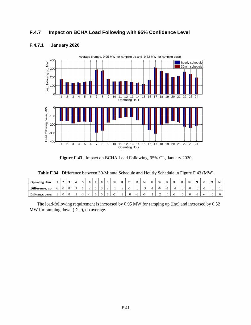
F.4.7 Impact on BCHA Load Following with 95% Confidence Level

F.4.7.1 January 2020

Figure F.43. Impact on BCHA Load Following, 95% CL, January 2020

Table F.34. Difference between 30-Minute Schedule and Hourly Schedule in Figure F.43 (MW)

Operating Hour 1 2 3 4 5 6 7 8 9 10 11 12 13 14 15 16 17 18 19 20 21 22 23 24

Difference, up 6 0 0 - 3 1 2 5 8 2 1 2 -1 0 3 -1 -6 -2 4 0 0 0 -1 0 1

Difference, down 1 0 0 - 4 - 3 - 1 0 0 0 -2 2 0 -1 -3 1 2 0 -1 0 0 -6 -4 0 6

The load-following requirement is increased by 0.95 MW for ramping up (Inc) and increased by 0.52 MW for ramping down (Dec), on average.

1 2 3 4 5 6 7 8 9 10 11 12 13 14 15 16 17 18 19 20 21 22 23 240

100

200

300

400

Operating Hour

Load

follo

win

g up

, MW

Average change, 0.95 MW for ramping up and -0.52 MW for ramping down

1 2 3 4 5 6 7 8 9 10 11 12 13 14 15 16 17 18 19 20 21 22 23 24-400

-300

-200

-100

0

Operating Hour

Load

follo

win

g do

wn,

MW

hourly schedule30min schedule

F.41

F.4.7.2 April 2020

Figure F.44. Impact on BCHA Load Following, 95% CL, April 2020

Table F.35. Difference between 30-Minute Schedule and Hourly Schedule in Figure F.44 (MW)

Operating Hour 1 2 3 4 5 6 7 8 9 10 11 12 13 14 15 16 17 18 19 20 21 22 23 24

Difference, up 1 7 2 4 -1 2 -1 4 1 2 3 -1 0 0 -1 0 -2 -2 -4 0 0 0 0 1

Difference, down 0 3 -1 1 2 0 0 -1 -1 1 2 3 3 -3 -2 -3 -1 -3 -1 -3 3 -10 -5 -3

The load-following requirement is increased by 0.59 MW for ramping up (Inc) and increased by 0.86 MW for ramping down (Dec), on average.

1 2 3 4 5 6 7 8 9 10 11 12 13 14 15 16 17 18 19 20 21 22 23 240

100

200

300

Operating Hour

Load

follo

win

g up

, MW

Average change, 0.59 MW for ramping up and -0.86 MW for ramping down

1 2 3 4 5 6 7 8 9 10 11 12 13 14 15 16 17 18 19 20 21 22 23 24-300

-200

-100

0

Operating Hour

Load

follo

win

g do

wn,

MW

hourly schedule30min schedule

F.42

F.4.7.3 August 2020

Figure F.45. Impact on BCHA Load Following, 95% CL, August 2020

Table F.36. Difference between 30-Minute Schedule and Hourly Schedule in Figure F.45 (MW)

Operating Hour 1 2 3 4 5 6 7 8 9 1 0 1 1 1 2 1 3 1 4 1 5 1 6 1 7 1 8 1 9 2 0 2 1 2 2 2 3 2 4

Difference, up 2 1 2 3 1 1 5 3 3 1 0 3 3 0 - 1 - 2 - 2 0 - 2 - 3 - 1 0 0 0

Difference, down 2 1 0 1 0 0 0 0 1 0 0 0 1 - 1 - 1 - 2 - 4 - 1 - 3 - 1 - 3 - 6 - 1 0

The load-following requirement is increased by 0.62 MW for ramping up (Inc) and increased by 0.7 MW for ramping down (Dec), on average.

1 2 3 4 5 6 7 8 9 10 11 12 13 14 15 16 17 18 19 20 21 22 23 240

100

200

300

400

Operating Hour

Load

follo

win

g up

, MW

Average change, 0.62 MW for ramping up and -0.7 MW for ramping down

1 2 3 4 5 6 7 8 9 10 11 12 13 14 15 16 17 18 19 20 21 22 23 24-300

-200

-100

0

Operating Hour

Load

follo

win

g do

wn,

MW

hourly schedule30min schedule

F.43

F.4.8 Impact on BCHA Load Following with 99.5% Confidence Level

F.4.8.1 January 2020

Figure F.46. Impact on BCHA Load Following, 99.5% CL, January 2020

Table F.37. Difference between 30-Minute Schedule and Hourly Schedule in Figure F.46 (MW)

Operating Hour 1 2 3 4 5 6 7 8 9 10 11 12 13 14 15 16 17 18 19 20 21 22 23 24

Difference, up 22 6 0 -6 6 10 2 9 9 3 0 -4 3 6 1 0 -7 -5 0 0 0 -2 -1 0

Difference, down 1 0 -3 -2 3 -2 0 -1 0 -6 1 -3 0 -11 -1 4 0 0 0 1 -5 -5 5 23

The load-following requirement is increased by 2.09 MW for ramping up (Inc) and increased by 0.06 MW for ramping down (Dec), on average.

1 2 3 4 5 6 7 8 9 10 11 12 13 14 15 16 17 18 19 20 21 22 23 240

100

200

300

400

500

Operating Hour

Load

follo

win

g up

, MW

Average change, 2.09 MW for ramping up and -0.06 MW for ramping down

1 2 3 4 5 6 7 8 9 10 11 12 13 14 15 16 17 18 19 20 21 22 23 24-400

-300

-200

-100

0

Operating Hour

Load

follo

win

g do

wn,

MW

hourly schedule30min schedule

F.44

F.4.8.2 April 2020

Figure F.47. Impact on BCHA Load Following, 99.5% CL, April 2020

Table F.38. Difference between 30-Minute Schedule and Hourly Schedule in Figure F.47 (MW)

Operating Hour 1 2 3 4 5 6 7 8 9 10 11 12 13 14 15 16 17 18 19 20 21 22 23 24

Difference, up 1 10 5 2 -25 1 -3 4 5 2 2 0 -1 0 0 4 -1 0 -7 -4 0 0 -1 0

Difference, down 1 10 -7 3 1 0 0 1 2 0 2 1 9 0 0 -1 -1 -2 0 -5 3 -37 -3 1

The load-following requirement is decreased by 0.18 MW for ramping up (Inc) and increased by 0.88 MW for ramping down (Dec), on average.

1 2 3 4 5 6 7 8 9 10 11 12 13 14 15 16 17 18 19 20 21 22 23 240

100

200

300

400

Operating Hour

Load

follo

win

g up

, MW

Average change, -0.18 MW for ramping up and -0.88 MW for ramping down

1 2 3 4 5 6 7 8 9 10 11 12 13 14 15 16 17 18 19 20 21 22 23 24-500

-400

-300

-200

-100

0

Operating Hour

Load

follo

win

g do

wn,

MW

hourly schedule30min schedule

F.45

F.4.8.3 August 2020

Figure F.48. Impact on BCHA Load Following, 99.5% CL, August 2020

Table F.39. Difference between 30-Minute Schedule and Hourly Schedule in Figure F.48 (MW)

Operating Hour 1 2 3 4 5 6 7 8 9 1 0 11 12 13 14 1 5 1 6 1 7 18 1 9 2 0 2 1 2 2 23 2 4

Difference, up 3 2 5 1 7 2 2 1 5 - 2 3 6 6 0 0 - 3 0 0 - 1 - 2 - 1 - 2 1 0

Difference, down 0 0 0 0 1 0 1 1 0 2 0 0 0 0 - 4 - 2 - 1 0 - 9 - 1 - 8 - 6 5 - 4

The load-following requirement is increased by 1.36 MW for ramping up (Inc) and increased by 1.01 MW for ramping down (Dec), on average.

1 2 3 4 5 6 7 8 9 10 11 12 13 14 15 16 17 18 19 20 21 22 23 240

100

200

300

400

500

Operating Hour

Load

follo

win

g up

, MW

Average change, 1.36 MW for ramping up and -1.01 MW for ramping down

1 2 3 4 5 6 7 8 9 10 11 12 13 14 15 16 17 18 19 20 21 22 23 24-400

-300

-200

-100

0

Operating Hour

Load

follo

win

g do

wn,

MW

hourly schedule30min schedule

F.46

F.4.9 Impact on TID Load Following with 95% Confidence Level

F.4.9.1 January 2020

Figure F.49. Impact on TID Load Following, 95% CL, January 2020

Table F.40. Difference between 30-Minute Schedule and Hourly schedule in Figure F.49 (MW)

Operating Hour 1 2 3 4 5 6 7 8 9 1 0 1 1 1 2 1 3 1 4 1 5 1 6 1 7 1 8 1 9 2 0 2 1 2 2 2 3 2 4

Difference, up 5 6 2 6 1 0 6 4 6 2 5 6 2 2 4 1 2 0 5 3 2 0 1 1 1

Difference, down -3 -2 -3 -10 - 2 0 -1 -1 -5 -3 -2 -1 -3 -7 -3 -4 -1 0 0 -3 -6 -4 -5 -5

The load-following requirement is increased by 3.37 MW for ramping up (Inc) and increased by 3.12 MW for ramping down (Dec), on average.

1 2 3 4 5 6 7 8 9 10 11 12 13 14 15 16 17 18 19 20 21 22 23 240

5

10

15

20

Operating Hour

Load

follo

win

g up

, MW

Average change, 3.37 MW for ramping up and -3.12 MW for ramping down

1 2 3 4 5 6 7 8 9 10 11 12 13 14 15 16 17 18 19 20 21 22 23 24-20

-15

-10

-5

0

Operating Hour

Load

follo

win

g do

wn,

MW

hourly schedule30min schedule

F.47

F.4.9.2 April 2020

Figure F.50. Impact on TID Load Following, 95% CL, April 2020

Table F.41. Difference between 30-Minute Schedule and Hourly Schedule in Figure F.50 (MW)

Operating Hour 1 2 3 4 5 6 7 8 9 10 11 12 13 14 15 16 17 18 19 20 21 22 23 24

Difference, up 0 1 3 6 2 4 0 3 3 1 2 1 2 0 0 0 0 1 -1 3 0 0 0 3

Difference, down -3 0 -3 0 0 -4 -1 -1 0 0 0 0 -1 -1 -4 -3 -2 -13 -1 -2 -1 -7 -3 -1

The load-following requirement is increased by 1.56 MW for ramping up (Inc) and increased by 2.15 MW for ramping down (Dec), on average.

1 2 3 4 5 6 7 8 9 10 11 12 13 14 15 16 17 18 19 20 21 22 23 240

5

10

15

20

25

Operating Hour

Load

follo

win

g up

, MW

Average change, 1.56 MW for ramping up and -2.15 MW for ramping down

1 2 3 4 5 6 7 8 9 10 11 12 13 14 15 16 17 18 19 20 21 22 23 24-25

-20

-15

-10

-5

0

Operating Hour

Load

follo

win

g do

wn,

MW

hourly schedule30min schedule

F.48

F.4.9.3 August 2020

Figure F.51. Impact on TID Load Following, 95% CL, August 2020

Table F.42. Difference between 30-Minute Schedule and Hourly Schedule in Figure F.51 (MW)

Operating Hour 1 2 3 4 5 6 7 8 9 10 11 12 13 14 15 16 17 18 19 20 21 22 23 24

Difference, up 0 0 1 3 2 2 2 3 2 1 3 1 5 1 0 0 1 0 0 0 0 0 3 1

Difference, down 0 - 1 - 1 - 1 0 0 0 0 0 0 -1 0 0 0 0 -2 -3 -2 -5 -5 -3 -2 -3 -1

The load-following requirement is increased by 1.27 MW for ramping up (Inc) and increased by 1.15 MW for ramping down (Dec), on average.

1 2 3 4 5 6 7 8 9 10 11 12 13 14 15 16 17 18 19 20 21 22 23 240

5

10

15

20

25

Operating Hour

Load

follo

win

g up

, MW

Average change, 1.27 MW for ramping up and -1.15 MW for ramping down

1 2 3 4 5 6 7 8 9 10 11 12 13 14 15 16 17 18 19 20 21 22 23 24-25

-20

-15

-10

-5

0

Operating Hour

Load

follo

win

g do

wn,

MW

hourly schedule30min schedule

F.49

F.4.10 Impact on TID Load Following with 99.5% Confidence Level

F.4.10.1 January 2020

Figure F.52. Impact on TID Load Following, 99.5% CL, January 2020

Table F.43. Difference between 30-Minute Schedule and Hourly Schedule in Figure F.52 (MW)

Operating Hour 1 2 3 4 5 6 7 8 9 10 11 12 13 1 4 15 1 6 17 18 19 20 21 22 23 24

Difference, up 7 13 6 1 7 15 14 5 12 1 9 7 3 4 7 3 1 1 1 12 11 2 1 1 2 1

Difference, down -11 -4 -5 -34 -4 0 -1 -3 -7 -4 -3 -2 -8 -12 -9 -10 -1 -1 -1 -5 -8 -5 -9 -8

The load-following requirement is increased by 6.87 MW for ramping up (Inc) and increased by 6.52 MW for ramping down (Dec), on average.

1 2 3 4 5 6 7 8 9 10 11 12 13 14 15 16 17 18 19 20 21 22 23 240

10

20

30

40

Operating Hour

Load

follo

win

g up

, MW

Average change, 6.87 MW for ramping up and -6.52 MW for ramping down

1 2 3 4 5 6 7 8 9 10 11 12 13 14 15 16 17 18 19 20 21 22 23 24-50

-40

-30

-20

-10

0

Operating Hour

Load

follo

win

g do

wn,

MW

hourly schedule30min schedule

F.50

F.4.10.2 April 2020

Figure F.53. Impact on TID Load Following, 99.5% CL, April 2020

Table F.44. Difference between 30-Minute Schedule and Hourly Schedule in Figure F.53 (MW)

Operating Hour 1 2 3 4 5 6 7 8 9 1 0 1 1 1 2 1 3 1 4 15 16 1 7 18 1 9 2 0 2 1 22 2 3 2 4

Difference, up 0 2 6 1 2 1 9 0 7 5 3 3 1 5 0 0 1 0 2 0 4 0 0 0 0

Difference, down -9 0 -8 - 1 0 -14 0 -2 0 0 0 0 - 2 - 3 -11 -10 - 3 -24 - 1 - 5 0 -19 - 6 - 2

The load-following requirement is increased by 2.48 MW for ramping up (Inc) and increased by 4.98 MW for ramping down (Dec), on average.

1 2 3 4 5 6 7 8 9 10 11 12 13 14 15 16 17 18 19 20 21 22 23 240

10

20

30

Operating Hour

Load

follo

win

g up

, MW

Average change, 2.48 MW for ramping up and -4.98 MW for ramping down

1 2 3 4 5 6 7 8 9 10 11 12 13 14 15 16 17 18 19 20 21 22 23 24-50

-40

-30

-20

-10

0

Operating Hour

Load

follo

win

g do

wn,

MW

hourly schedule30min schedule

F.51

F.4.10.3 August 2020

Figure F.54. Impact on TID Load Following, 99.5% CL, August 2020

Table F.45. Difference between 30-Minute Schedule and Hourly Schedule in Figure F.54 (MW)

Operating Hour 1 2 3 4 5 6 7 8 9 10 11 12 13 14 15 16 17 18 19 20 2 1 2 2 23 24

Difference, up 0 0 1 12 2 6 8 7 3 1 6 2 30 2 0 0 2 0 0 0 - 1 0 22 2

Difference, down -2 -1 -3 -2 0 0 0 0 0 0 0 0 0 0 0 -4 -4 -3 -6 -6 -10 -26 -8 -5

The load-following requirement is increased by 4.39 MW for ramping up (Inc) and increased by 3.28 MW for ramping down (Dec), on average.

1 2 3 4 5 6 7 8 9 10 11 12 13 14 15 16 17 18 19 20 21 22 23 240

10

20

30

40

50

Operating Hour

Load

follo

win

g up

, MW

Average change, 4.39 MW for ramping up and -3.28 MW for ramping down

1 2 3 4 5 6 7 8 9 10 11 12 13 14 15 16 17 18 19 20 21 22 23 24-60

-40

-20

0

Operating Hour

Load

follo

win

g do

wn,

MW

hourly schedule30min schedule

F.52

F.4.11 Impact on SMUD Load Following with 95% Confidence Level

F.4.11.1 January 2020

Figure F.55. Impact on SMUD Load Following, 95% CL, January 2020

Table F.46. Difference between 30-Minute Schedule and Hourly Schedule in Figure F.55 (MW)

Operating Hour 1 2 3 4 5 6 7 8 9 10 11 12 13 14 15 16 17 18 19 20 21 22 23 24

Difference, up 0 1 1 0 1 3 3 2 0 -1 2 1 1 0 0 2 -2 1 2 0 0 0 0 0

Difference, down 1 -1 -2 -4 0 0 0 0 0 -2 1 -2 -1 -1 -3 -1 0 0 -1 -1 -5 -2 2 -3

The load-following requirement is increased by 0.75 MW for ramping up (Inc) and increased by 1.1 MW for ramping down (Dec), on average.

1 2 3 4 5 6 7 8 9 10 11 12 13 14 15 16 17 18 19 20 21 22 23 240

20

40

60

80

100

Operating Hour

Load

follo

win

g up

, MW

Average change, 0.75 MW for ramping up and -1.1 MW for ramping down

hourly schedule30min schedule

1 2 3 4 5 6 7 8 9 10 11 12 13 14 15 16 17 18 19 20 21 22 23 24-100

-80

-60

-40

-20

0

Operating Hour

Load

follo

win

g do

wn,

MW

F.53

F.4.11.2 April 2020

Figure F.56. Impact on SMUD Load Following, 95% CL, April 2020

Table F.47. Difference between 30-Minute Schedule and Hourly Schedule in Figure F.56 (MW)

Operating Hour 1 2 3 4 5 6 7 8 9 1 0 1 1 1 2 13 1 4 1 5 1 6 1 7 1 8 1 9 2 0 2 1 2 2 2 3 2 4

Difference, up 0 2 0 2 0 1 4 1 3 3 1 1 1 1 -1 0 0 0 -1 0 0 -1 0 0

Difference, down -3 1 0 0 0 0 0 0 0 0 1 0 1 0 -2 -1 -2 -2 0 0 -2 -2 -2 1

The load-following requirement is increased by 0.64 MW for ramping up (Inc) and increased by 0.55 MW for ramping down (Dec), on average.

1 2 3 4 5 6 7 8 9 10 11 12 13 14 15 16 17 18 19 20 21 22 23 240

50

100

150

Operating Hour

Load

follo

win

g up

, MW

Average change, 0.64 MW for ramping up and -0.55 MW for ramping down

hourly schedule30min schedule

1 2 3 4 5 6 7 8 9 10 11 12 13 14 15 16 17 18 19 20 21 22 23 24-150

-100

-50

0

Operating Hour

Load

follo

win

g do

wn,

MW

F.54

F.4.12 August 2020

Figure F.57. Impact on SMUD Load Following, 95% CL, August 2020

Table F.48. Difference between 30-Minute Schedule and Hourly Schedule in Figure F.57 (MW)

Operating Hour 1 2 3 4 5 6 7 8 9 10 11 12 13 14 15 16 17 18 19 20 21 22 23 24

Difference, up 0 0 1 0 0 3 3 2 1 1 0 1 2 0 1 -1 0 0 0 0 0 0 0 0

Difference, down -1 1 0 0 0 0 0 0 0 0 0 0 0 0 0 0 -2 -2 -3 -1 -1 -2 -3 0

The load-following requirement is increased by 0.55 MW for ramping up (Inc) and increased by 0.54 MW for ramping down (Dec), on average.

1 2 3 4 5 6 7 8 9 10 11 12 13 14 15 16 17 18 19 20 21 22 23 240

50

100

150

Operating Hour

Load

follo

win

g up

, MW

Average change, 0.55 MW for ramping up and -0.54 MW for ramping down

1 2 3 4 5 6 7 8 9 10 11 12 13 14 15 16 17 18 19 20 21 22 23 24-150

-100

-50

0

Operating Hour

Load

follo

win

g do

wn,

MW

hourly schedule30min schedule

F.55

F.4.13 Impact on SMUD Load Following with 99.5% Confidence Level

F.4.13.1 January 2020

Figure F.58. Impact on SMUD Load Following, 99.5% CL, January 2020

Table F.49. Difference between 30-Minute Schedule and Hourly Schedule in Figure F.58 (MW)

Operating Hour 1 2 3 4 5 6 7 8 9 10 11 12 13 14 15 16 17 18 19 20 21 22 23 24

Difference, up 0 3 0 4 0 1 8 1 0 2 4 1 1 0 0 6 -1 -1 1 0 0 -2 0 2

Difference, down 0 -5 -1 -3 -1 0 0 1 -1 -2 -1 -6 0 0 -4 -2 0 -1 0 -4 -2 -5 1 0

The load-following requirement is increased by 1.18 MW for ramping up (Inc) and increased by 1.43 MW for ramping down (Dec), on average.

1 2 3 4 5 6 7 8 9 10 11 12 13 14 15 16 17 18 19 20 21 22 23 240

50

100

150

Operating Hour

Load

follo

win

g up

, MW

Average change, 1.18 MW for ramping up and -1.43 MW for ramping down

1 2 3 4 5 6 7 8 9 10 11 12 13 14 15 16 17 18 19 20 21 22 23 24-150

-100

-50

0

Operating Hour

Load

follo

win

g do

wn,

MW

hourly schedule30min schedule

F.56

F.4.13.2 April 2020

Figure F.59. Impact on SMUD Load Following, 99.5% CL, April 2020

Table F.50. Difference between 30-Minute Schedule and Hourly Schedule in Figure F.59 (MW)

Operating Hour 1 2 3 4 5 6 7 8 9 1 0 1 1 1 2 1 3 1 4 1 5 1 6 1 7 1 8 1 9 2 0 2 1 2 2 2 3 2 4

Difference, up -1 5 -1 6 1 0 9 0 4 6 1 1 1 0 0 - 1 1 2 - 4 1 0 0 0 1

Difference, down -6 2 -1 0 0 0 1 1 1 - 2 1 0 0 - 2 1 - 1 0 0 0 0 - 2 0 - 5 1

The load-following requirement is increased by 1.27 MW for ramping up (Inc) and increased by 0.48 MW for ramping down (Dec), on average.

1 2 3 4 5 6 7 8 9 10 11 12 13 14 15 16 17 18 19 20 21 22 23 240

50

100

150

Operating Hour

Load

follo

win

g up

, MW

Average change, 1.27 MW for ramping up and -0.48 MW for ramping down

1 2 3 4 5 6 7 8 9 10 11 12 13 14 15 16 17 18 19 20 21 22 23 24-150

-100

-50

0

Operating Hour

Load

follo

win

g do

wn,

MW

hourly schedule30min schedule

F.57

F.4.13.3 August 2020

Figure F.60. Impact on SMUD Load Following, 99.5% CL, August 2020

Table F.51. Difference between 30-Minute Schedule and Hourly Schedule in Figure F.60 (MW)

Operating Hour 1 2 3 4 5 6 7 8 9 1 0 1 1 1 2 1 3 1 4 1 5 1 6 1 7 1 8 1 9 2 0 2 1 2 2 23 2 4

Difference, up 0 0 1 0 0 4 2 5 2 0 - 1 0 5 0 2 0 0 0 - 1 0 - 1 0 0 0

Difference, down -1 1 0 -1 0 0 0 1 0 0 0 0 0 0 0 0 0 - 4 - 3 - 2 - 3 - 1 -9 0

The load-following requirement is increased by 0.73 MW for ramping up (Inc) and increased by 0.97 MW for ramping down (Dec), on average.

F.5 Reserve Shifting Analyses Conclusions

A modified algorithm to calculate the load-following requirements for BAs implementing half-hour wind transfer schedules is developed and tested on the NWPP system models. Five wind transfers are defined with different capacities, including BPA-PGN, BPA-PSE, BPA-BCHA, BPA-TID and BPA-SMUD. For the half-hour wind schedules, a T−31 persistence model is used to generate the first half-hour wind schedule for the next operating hour and a T−1 persistence model is used to generate the second half-hour wind schedule for the next hour. With the five wind transfers implemented simultaneously, the load-following requirements for the source BA and sink BAs are calculated and then compared with the original hourly schedule scenario. From the simulation results, it is observed that the load-following requirements are decreased for both ramping up and ramping down requirements in the source BA. The average increased magnitude ranges from 25.61 to 58.19 MW, varying in different study months and with different confidence levels. In general, the load-following requirements for the sink BAs are increased as a result of the half-hour wind schedule.

1 2 3 4 5 6 7 8 9 10 11 12 13 14 15 16 17 18 19 20 21 22 23 240

50

100

150

200

Operating Hour

Load

follo

win

g up

, MW

Average change, 0.73 MW for ramping up and -0.97 MW for ramping down

1 2 3 4 5 6 7 8 9 10 11 12 13 14 15 16 17 18 19 20 21 22 23 24-200

-150

-100

-50

0

Operating Hour

Load

follo

win

g do

wn,

MW

hourly schedule30min schedule

F.58

PNNL-22877

Distribution

No. of No. of Copies Copies

# Name Organization Address City, State and ZIP Code

# Organization Address City, State and ZIP Code Name Name Name Name Name (#)

# Name Organization Address City, State and ZIP Code

# Foreign Distribution # Name

Organization Address Address line 2 COUNTRY

# Local Distribution Pacific Northwest National Laboratory Name Mailstop Name Mailstop Name Mailstop Name Mailstop Name (PDF)

Distr.1