An Investigation of Objective and Subjective Performance Measures: New Evidence from the Education Sector∗

Brian A. Jacob Harvard University and NBER

Lars Lefgren

Brigham Young University

First Draft: January 2005

VERY PRELMINARY: COMMENTS WELCOME – PLEASE DO NOT CITE

∗ We would like to thank Joseph Price and J.D. LaRock for their excellent research assistance. We thank Doug Staiger, Chris Hansen, Frank McIntrye, and seminar participants at UC Berkeley, Northwestern, BYU, and the University of Virginia for helpful comments. All remaining errors are our own. Jacob can be contacted at: John F. Kennedy School of Government, Harvard University, 79 JFK Street, Cambridge, MA 02138; email: brian_jacob@harvard.edu. Lefgren can be contacted at: Department of Economics, Brigham Young University, 130 Faculty Office Building, Provo, UT 84602-2363; email: l-lefgren@byu.edu.

An Investigation of Objective and Subjective Performance Measures: New Evidence from the Education Sector

Abstract Subjective supervisor evaluations play a large role in promotion and retention decisions in a wide variety of occupations. In this paper, we examine the relationship between objective and subjective measures of performance in the education sector. Specifically, we ask three questions: (1) Can principals identify effective teachers defined as those who produce the largest improvement on standardized exams? (2) Do principals discriminate against teachers with certain characteristics? (3) How do principals form assessments of teachers? To answer these questions, we combine a rich set of administrative data that links student achievement scores to individual teachers with a survey of principals. We find that principals can identify the best and worst teachers in their schools fairly well, but have less ability to distinguish between teachers in the middle of the ability distribution. In all cases, however, objective value-added measures are better able to predict actual effectiveness than principal reports. We find some evidence that principals discriminate against male and untenured teachers and in favor of teachers with whom they have a closer personal relationship. Finally, we find that in forming their assessments principals focus disproportionately on the recent experience of the teacher and are imperfect Bayesians, failing to appropriately account for the noisy performance signals they receive.

1

"I shall not today attempt further to define the kinds of material I understand to be embraced . . . [b]ut I know it when I see it.”

Justice Potter Stewart (trying to define obscenity)

I. Introduction

Subjective supervisor evaluations play a large role in promotion and retention decisions

in a wide variety of occupations. In professions that involve complex jobs with multiple

outcomes that are difficult to observe, firms most often rely on subjective evaluations of

employees (Prendergast 1999). Despite their widespread use, subjective evaluations have a

number of drawbacks, including the tendency to result in very lenient ratings and to increase the

possibility of supervisor bias (Prendergast 1999). Perhaps most importantly, prior studies in

organizational management and psychology suggest that subjective ratings are only weakly

related with objective measures of job performance. Unfortunately, the majority of these studies

are based on selective samples, do not account for measurement error and focus on occupations

with relatively easy-to-measure outputs such as sales.

In this paper, we examine the relationship between objective and subjective measures of

performance in the education sector. Specifically, we ask three questions: (1) Can principals

identify effective teachers defined as those who produce the largest improvement on

standardized exams? (2) Do principals discriminate against teachers with certain characteristics?

(3) How do principals form assessments of teachers?

Education has several features that make it an excellent context in which to examine

subjective performance measures. First, standardized test scores provide a plausible and easily

available measure of objective teacher performance (along at least one dimension). Indeed, there

is a well-established literature that seeks to create measures of school and teacher performance

2

on the basis of standardized test scores. Second, a host of characteristics including experience,

educational background and demographics are available for teachers, which allow one to explore

more carefully how principals assess teachers including, for example, issues of discrimination.

A major drawback of studying subjective performance measurement within education is that in

most public schools, formal principal evaluations have no impact on teacher compensation, so

they are often not taken seriously by principals or teachers. To avoid this problem, we conducted

an independent, confidential survey of principals to elicit their true views of the teachers in their

school.

Moreover, the relationship between subjective and objective performance evaluation is

particularly important in the field of education. There is a widespread perception in education

that “good teaching” is very hard to measure. Decades of education production function research

have found little association between teacher characteristics such as certification or experience

and student outcomes (Hanushek 1986, 1997). At the same time, several studies have

documented substantial variation among teachers in their ability to raise student achievement

(Murnane 1975, Hanushek 1992, Hanushek & Rivkin, 2004, Aaronson et. al. 2004, Rockoff

2004). It thus appears that certain teachers are indeed more effective than others, but that this

ability is simply not correlated with any commonly measured indicator of teacher quality. A

common perception among educators is that high quality teaching is like obscenity – it cannot

easily be defined, but one “knows it when [one] see it.” 1 Unfortunately, there is little evidence

to confirm or disprove this view.

The ability of principals to identify effective teachers has practical implications as well.

While it is difficult for public school principals to hire or fire tenured teachers, it is much easier

1 In 1964, Justice Potter Stewart tried to explain "hard-core" pornography, or what is obscene, by saying, "I shall not today attempt further to define the kinds of material I understand to be embraced . . . [b]ut I know it when I see it.” Jacobellis v. Ohio, 378 U.S. 184, 197 (1964).

3

to release new teachers deemed ineffective. Additionally, they have a large number of informal

levers to reward or sanction teachers. For example, they can express their dissatisfaction with a

teacher’s performance and engage in repeated observation of that teacher—a process which most

instructors find highly stressful. They can also encourage incompetent teachers to transfer to a

different school. Conversely, principals can reward their best teachers by assigning to them

leadership roles with a school (e.g. reading specialist). If principals can identify effective

teachers, then one may feel more comfortable allowing principal evaluations to play a greater

role in determining pay and promotion.

In this paper, we analyze objective and subjective performance evaluations for over 200

elementary school teachers. With the assistance of a public school district in the western United

States, we were able to link achievement data for students from 1997-2003 with detailed

administrative data on their teachers, including age, experience, educational background, license

and certification information. We administered confidential surveys to principals in 13

elementary schools asking them to not only rate each teacher in their school on a variety of

different dimensions, but also judge the confidence of their assessments and describe the various

ways in which they monitored teachers.

To preview our results, we find that principals can identify the best and worst teachers in

their schools fairly well, but have less ability to distinguish between teachers in the middle of the

ability distribution. In all cases, however, objective value-added measures are better able to

predict actual effectiveness than principal reports. We find some evidence that principals

discriminate against male and untenured teachers and in favor of teachers with whom they have a

closer personal relationship. Finally, we find that in forming their assessments principals focus

4

disproportionately on the recent experience of the teacher and are imperfect Bayesians, failing to

appropriately account for the noisy performance signals they receive.

The remainder of the paper proceeds as follows. In Section II, we review the literature on

objective and subjective performance evaluation. In Section III, we describe our data and in

Section IV outline how we construct the different measures of teacher effectiveness. The main

results together with the empirical methodology are presented in Section V and VI. We conclude

in Section VII.

II. Prior Literature

There is a long history of studies in organizational management, psychology and

personnel economics that seek to determine the extent to which subjective supervisor ratings

match objective measures of employee performance.2 Overall, this research suggests that there

is a relatively weak relationship between subjective ratings and objective performance and that

supervisor ratings are influenced by a number of demographic and interpersonal factors. In a

meta-analysis of 23 studies of workers in a variety of jobs, Heneman (1986) found that

supervisor ratings and objective performance were correlated 0.27 after correcting for sampling

error and attenuation bias. A subsequent meta-analysis by Bommer et al. (1995) that included a

larger percentage of sales jobs found a corrected mean correlation of 0.39.

The other main finding from this literature is that supervisor evaluations are often

influenced by a number of non-performance factors such as the age and gender of the supervisor 2 Studies about subjective ratings and objective performance have examined a number of different occupations, including vocational rehabilitation counselors (Alexander & Wilkins, 1988); field employees at a telephone company (Bishop, 1974); administrative and investigative personnel in a law enforcement agency (Bolino & Turnley, 2003); operators, technicians, and dispatch clerks at a telephone company (Duarte, Goodson & Klich, 1993); internal auditors (Fogarty & Kalbers, 1993); mechanical, maintenance, and field service worker at a gas company (Hoffman, Nathan, & Holden, 1991); registered nurses (Judge & Ferris, 1993); sales employees at a data processing company (Kingstrom & Mainstone, 1985); accountants (Ross & Ferris, 1981); and communications workers (Varma & Stroh, 2001).

5

and subordinate and the likeability of the subordinate influence subjective performance

evaluation. For example, many studies document that that supervisors rate employees that they

like more highly than others, conditional on objective performance measures (Alexander &

Wilkins, 1982; Bolino & Turnley, 2003; Heneman, Greenberger & Anonyuo, 1989; Lefkowitz,

2000; Wayne & Ferris, 1990). Similarly, some studies have found that supervisors will give

higher ratings to employees that they perceive as similar to themselves along dimensions such as

personality, background, and more obvious characteristics such as gender (Heneman,

Greenberger & Anonyuo, 1989; Varma & Stroh, 2001). Prendergast (1999) observes that in

theory such biases create an incentive for employee’s to engage in inefficient “influence”

activities. Wayne and Ferris (1990) provide some empirical support for this hypothesis, finding

that certain types of “influence tactics” such as ingratiation of the supervisor had a salutary effect

on performance ratings.3

While these findings are suggestive, this literature has many limitations. First, most of

the studies involve extremely small samples and, more importantly, often focus on a highly

selective (sometimes voluntary) sample. Second, many of the studies involve occupations where

worker productivity may be relatively easy to observe such as sales, and thus may not provide

much insight regarding the relationship for more complex occupations. Third, these studies

generally do not account for selection issues, so that the objective performance measures are

likely biased estimates of an employee’s “true” productivity. In a seminal study of vocational

3 Studies in this literature have also found that supervisor traits and behaviors can affect the validity of subjective ratings (Bommer et al, 1995; Fogarty & Kalbers, 1993; Heneman, Wexley & Moore, 1987; Judge & Ferris, 1993; Podsakoff, et al, 1995). For instance, several studies note that a supervisor’s experience, opportunity to observe employees, the number of subordinates, fa miliarity with the rating criteria, and other personal qualities can all influence the link between subjective ratings and objective performance (Heneman, 1986; Heneman, Wexley & Moore, 1987; Judge & Ferris, 1993). Others find that the format of the performance rating makes a difference, with more detailed ratings that use multiple criteria, as opposed to overall ratings, yielding more accurate links to objective performance (Heneman, 1986; Heneman, Wexley & Moore, 1987). In addition, ratings that compare the relative performance of employees, rather than evaluate them against a global standard, appear to be more accurate (Bommer, Johnson, Rich, Podsakoff, et al, 1995; Fogarty & Kalbers, 1993; Heneman, 1986).

6

rehabilitation counselors, for example, the researchers use the number of applications for service

completed and the number of cases closed by the counselor as measures of objective productivity

(Alexander and Wilkins 1982). To the extent that there is any non-random sorting of clients

across rehabilitation centers or counselors, these measures are likely biased. Fourth, these

studies do not adequately account for measurement error, which will tend to attenuate the

estimated correlations. Finally, because supervisors are generally asked to either provide a

single overall rating of the employee or to rate the employee on a number of different dimensions

which are then averaged to come up with a single composite measure, it is not clear that the

subjective and objective measures in these studies are identifying the same underlying construct,

which may lead the correlations to be biased downward.4

There is a parallel, though apparently independent, strand of research in the education

field.5 This research generally finds that the correlation between principal-based teacher

evaluations and student achievement gains is roughly 0.20 (Medley and Coker 1987, Peterson

1987, 2000). This literature concludes that principals cannot identify good teachers and

therefore traditional principal-based teacher evaluations should be abandoned or dramatically

changed. Interestingly, two notable studies outside the field of education find similar patterns

but interpret the results somewhat differently. Murnane (1975) and Armor et al. (1976) both

found principal evaluations of teachers predicted student achievement, even after conditioning on

prior test scores and a host of other student and classroom level demographic controls. While it

is difficult to directly compare these results to the education studies, the magnitude of the

4 Bommer, Johnson, Rich, Podsakoff, et al. (1995) emphasize the potential importance of this issue, noting that in the three studies they found where objective and subjective measures tapped precisely the same performance dimension, the mean corrected correlation was 0.71. 5 Interestingly, the education studies are not referenced in the organizational management or psychology literature despite the similarity of research objective and approach.

7

relationship appears to be modest.6 Nonetheless, these studies conclude that the existence of a

significant association suggests that (a) classroom fixed effect measures do reflect teacher quality

(as opposed to other classroom specific variables) and (b) principals can identify effective

teachers.7

These studies suffer from many of the same shortcomings as those in organizational

management and psychology. Most of the studies involve extremely small samples and, more

importantly, often focus on a highly selective (sometimes voluntary) sample. Few of these

studies attempt to correct for the measurement error in the student achievement measures.

Finally, these studies do not specifically ask principals about teachers’ ability to raise student

achievement, making it impossible to distinguish the hypothesis that principals cannot identify

effective teachers from the hypothesis that principals simply value other teacher characteristics.8

III. Data

The data for this study come from a mid-size school district located in the western United

States.9 With the assistance of the district, we were able to link student and teacher data. The

student data includes all of the common demographic variables as well as standardized

6 Murnane (1975) found that for third grade math, an increase in the principal rating of roughly 1 standard deviation was associated with an increase of 1.3 standard scores (or 0.125 standard deviations). The magnitude of the reading effect was somewhat smaller. Armor et. al. (1976) found that a one standard deviation increase in teacher effectiveness led to a 1-2 point raw score gain (although it is not possible to calculate the effect size given the available information in the study). 7 The few studies that examine the correlation between principal evaluations and other measures of teacher performance, such as parent or student satisfaction, find similarly weak relationships (Peterson 1987, 2000). These studies also document the prevalence of leniency and compression bias in principal evaluations (Medley and Coker 1987, Peterson 1987, Bridges 1992). Principal evaluations tend to be extremely generous with nearly all teachers receiving satisfactory or exemplary ratings. Digilio (1984) reports that only 0.003 percent of teachers in Baltimore, Philadelphia, and Montgomery County, Maryland, were evaluated as unsatisfactory in 1983. While teachers express concern regarding favoritism on the part of administrators, there is little empirical evidence as to whether, or to what extent, principal relationships with teachers are reflected in teacher evaluations (Peterson 2000). 8 Medley and Coker (1987) are unique in specifically asking principals to evaluate a teacher’s ability to improve student achievement. They find that the correlation with these subjective evaluations are no higher than with an overall principal rating. 9 The district has requested to remain anonymous.

8

achievement scores, and allows us to track the same student over time. The teacher data includes

a variety of teacher characteristics that have been used in previous studies, such as age,

experience, educational attainment, undergraduate and graduate institution attended, and license

and certification information. We link this data to principal evaluations of teacher performance

on a variety of different dimensions that we collected in a survey administered to elementary

principals in 2002-03.

To provide some context for the analysis, Table 1 shows summary statistics from the

district. While the students in the district are predominantly white (73 percent), there is a

reasonable degree of heterogeneity in terms of ethnicity and socioeconomic status. Latino

students comprise 21 percent of the elementary population and nearly half of all students in the

district (48 percent) receive free or reduced price lunch. Achievement levels in the district are

almost exactly at the average of the nation (49th percentile on the Stanford Achievement Test).

The primary unit of analysis in this study is the teacher. To ensure that we could link

student achievement data to the appropriate teacher, we limit our sample to elementary teachers

who were teaching a core subject10 during the 2002-03 academic year. We exclude kindergarten

and first grade teachers because achievement exams are not available for these students.11

Our sample consists of 202 teachers in grades 2 - 6. Like the students, the teachers in our

sample are fairly representative of elementary school teachers nationwide. Only 16 percent of

teachers in our sample are men. The average teacher is 42 years old and has roughly 12 years of

experience teaching. The vast majority of teachers attended the main local university, while 10

percent attended another instate college and six percent attended a school out of state. 17 percent

10 We exclude non-core teachers such as music teachers, gym teachers and librarians. 11 Achievement exams are given to students in grades one to six. In order to create a value-added measure of teacher effectiveness, it is necessary to have prior achievement information for the student, which eliminates kindergarten and first grade students.

9

of teachers have a MA degree or higher, and the vast majority of teachers are licensed in either

early childhood education or elementary education. Finally, 8 percent of the teachers in our

sample taught in a mixed-grade classroom in 2002-03 and 5 percent were in a “split” classroom

with another teacher.

In this district, elementary students take a set of “Core” exams in reading and math in

grades 1 to 8.12 These multiple-choice criterion-referenced exams cover topics that are closely

linked to the district learning objectives and goals. While student achievement results have not

been directly linked to rewards or sanctions until recently, the results of the Core exams are

distributed to parents and published annually. Citing these factors, district officials suggest that

teachers and principals have focused on this exam even before the recent passage of the federal

accountability legislation No Child Left Behind.

IV. Measures of Teacher Quality

This section describes how we create the subjective and objective measures of teacher

performance used in this study.

Subjective (Principal-Based) Measures of Teacher Effectiveness

To obtain subjective performance assessments, we administered a survey to all

elementary school principals in February 2003 asking them to evaluate their teachers along a

variety of dimensions (see Appendix A for a sample survey form).13 Principals were asked to

12 Students in select grades have recently begun to take a science exam as well. The district also administered the Standford Achievement Test (a national, norm-referenced exam) to students in grades three, five and eight over this period. 13 In this district, principals conduct formal evaluations annually for new teachers and every third year for tenured teachers. However, prior studies have found such formal evaluations suffer from considerable compression with nearly all teachers being rated very highly. These evaluations are also part of a teacher’s personnel file and it was not possible to obtain access to these without permission of the teachers.

10

rate teachers on a scale from 1 (inadequate) to 10 (exceptional). Importantly, principals were

asked to not only provide a rating of overall teacher effectiveness, but also to assess a number of

specific teacher characteristics including dedication and work ethic, classroom management,

parent satisfaction, positive relationship with administrators and ability to raise math and reading

achievement. Principals were assured that their responses would be completely confidential and

would not be revealed to the teachers or to any other school district employee.

Table II presents the summary statistics of each rating. It is clear that even these

informal, confidential and non-binding evaluations suffer from substantial compression and

leniency bias. The average rating is 8.07 and the range of scores from the 10th to the 90th

percentile only extends from 6 to 10. Less than 2 percent of the teachers were rated below a 5

and roughly 75 percent were rated between 7 and 9. While there was some heterogeneity across

principals, all awarded quite high ratings. Indeed, the average rating for the least generous

principal was 6.7. At the same time, however, there appears to be considerable variation in

ratings within school. Figure I shows histograms of math and reading ratings where each

teacher’s rating has been normalized by subtracting the median rating within the school for that

same item. It appears that principal ratings within school are roughly normally distributed with

five to six relevant categories.14

As the subjective measure of teacher effectiveness, we rely primarily on the principal

ratings of a teacher’s ability to raise math or reading scores. Because principal ratings differ in

terms of the degree of leniency and compression, we normalize the ratings by subtracting from

each rating the principal-specific mean for that question and dividing by the standard deviation.

We use all of the items to measure principal’s subjective assessment of different teacher

qualities. Table III shows the correlation between the individual items of the survey. The 14 The category of three below the median includes the few very low scores.

11

correlations between many of the individual principal ratings are quite high, suggesting that

many of the items likely reflect the same or similar dimensions of teacher performance. For

example, the correlation between teacher organization and classroom management exceeds 0.7;

the correlation between student satisfaction and the degree to which a teacher is a positive role

model is similarly large.

To reduce the dimensionality of the principal ratings, we performed an exploratory factor

analysis which yielded three factors.15 Table IV shows the factor loadings for the factors.16 The

first factor clearly measures student satisfaction, with high loadings on principal ratings of

student satisfaction and teacher as role model. The second factor appears to capture what might

be described as traditional “teaching ability,” with high loadings on classroom management,

organization and ability to influence student math and reading scores. The third factor captures a

teacher’s collegiality, with high loadings on the items that ask principals to assess the teacher’s

relationship with colleagues and administrators.

Objective (Student Achievement-Based) Measures of Teacher Effectiveness

The primary challenge to estimating measures of teacher effectiveness using student

achievement data involves the potential for non-random assignment of students to classes.

Following the standard practice in this literature, we estimate value-added models that control for

a wide variety of observable student and classroom characteristics including prior achievement

15 Because the principal evaluation of parent satisfaction may be highly correlated with the parent request measure that is included in some models, we exclude this item in creating the principal factors. While this increases the significance of the parental request measure, it does not impact any of the other estimates in the model. As an additional check, we create a second set of principal measures that are purged of the parent satisfaction information by regressing the factors created above on the parental satisfaction item. We then use the residuals from these regressions as factors that are by construction orthogonal to the principal’s view of parent satisfaction. Aside from increasing the significance of the parent request measures, the results from using these factors are comparable to the results based on the original factors. 16 These factors were derived from a Maximum Likelihood factor analysis method limited to three factors with a Promax rotation.

12

measures and, in some specifications, student fixed effects (see, for example, Aaronson et al.

2004, Rockoff 2004 and Hanushek and Rivkin 2004). Specifically, we estimate models like the

following:

(1) ijkt jt it t k j jt ijkty C X ψ φ δ α ε= Β + Γ + + + + +

where i indexes students, j indexes teachers, k indexes school, and t indexes year. The outcome

measure, y , is a student’s score on a math or reading exam. The scores are reported as the

percentage of items the student answered correctly. As mentioned earlier, we normalize

achievement scores to be mean zero and with a standard deviation of one within each year and

grade.

The vector X consists of the following student characteristics: age, race, gender, free-

lunch eligibility, special education placement, limited English proficiency status, prior math

achievement, prior reading achievement, and grade fixed effects. C is a vector of classroom

measures that include indicators for class size and average student characteristics. tψ and kφ are

a set of year and school fixed effects respectively. Teacher j’s contribution to value added is

captured by the 'j sδ .17 jtα is an error term that is common to all students in teacher j’s

classroom in period t (e.g., adverse testing conditions faced by all students in a particular class

such as a barking dog). ijktε is an error term that takes into account the student’s idiosyncratic

error.

To the extent that principals evaluate a teacher relative to other teachers within the

school, a value-added indicator that measures effectiveness relative to a district rather than

17 Our value-added models implicitly assume that teacher quality does not change with experience. While recent evidence indicates that quality increases with experience, particularly in the first few years of teaching (see Rockoff 2004), we believe this is a reasonable assumption for the relatively short time period that we examine. In future versions of this paper, we plan to estimate models that allow quality to change with experience.

13

school average will be biased downward. 18 To insure we identify estimates of teacher quality

relative to other teachers within the same school, we examine teachers who are in their most

recent school (i.e. for the small number of switching teachers, we drop observations from their

first school), include school fixed effects and then constrain the teacher fixed effects to sum to

zero within each school.19

To account for unobservable, time- invariant student characteristics, we estimate models

that include student fixed effects iλ with either achievement levels or gains as the dependent

variable:

(2) ijkt jt it t k j jt i ijkty C X ψ φ δ α λ ε= Β + Γ + + + + + +

(3) 1ijkt ijkt jt it t k j jt i ijkty y C X ψ φ δ α λ ε−− = Β + Γ + + + + + +

These models account for all unobservable fixed characteristics, including student

motivation and family involvement, but do not control for time-varying unobservables. Note

that in specification (2) the covariates include lagged achievement measures. In specification (3)

lagged achievement measures are not included. While there is no way (short of randomly

assigning students and teachers to classrooms) to completely rule out the possibility of such

selection bias, several pieces of evidence suggest that such non-random sorting is unlikely to

produce a substantial bias in this case.20 First, with the assistance of district administrators, we

have conducted detailed interviews with principals to ascertain exactly how students are assigned

to classrooms and to explicitly examine how the assignment process may influence our

18 Typical value added models that simply contain school fixed effects identify teacher quality relative to all teachers (or some omitted teacher) in the district. 19 The fact that principals are likely using different scales when evaluating teachers makes any correlation between supervisor ratings and a district-wide productivity measure largely uninformative (even in the case where principals were attempting to evaluate their own teachers relative to all others in the district). 20 Note that the existence of bias presumes that parents can identify which teacher will be most effective for his or her child, which is doubtful given the results on principals presented here and the results on parental preferences presented in Jacob and Lefgren (2005).

14

estimates. In many schools, particularly in sixth grade, it turns out that students are tracked for

math instruction. In these cases, we do not construct value-added measures for math

achievement, focusing only on the relationship between principal ratings and teacher value-

added for reading, which is never tracked across classrooms.21 Second, we show that once we

eliminate these tracked classes, teacher effects that include virtually no controls are highly

correlated with value-added measures that include a much more detailed set of controls,

suggesting that students are not systematically sorting into classrooms along observable

dimensions and thus providing some assurance that they may not be sorting along unobservable

dimensions either.22 Finally, with the assistance of school principals, we examine the only other

avenue for non-random assignment – parent requests. While many principals attempt to honor

these requests, the principals also attempt to balance ability levels across classrooms, limiting the

impact of non-random sorting.23 Conditional on initial achievement and basic demographics, we

find that the students whose parents submit requests do not perform significantly better or worse

than non-requesting students. This suggests that teacher assignment on the basis of parent

requests is unlikely to be highly correlated with unobserved student ability.

While we make use of extremely rich panel data on student achievement, the value-added

specifications described above have distinct limitations nonetheless. As Todd and Wolpin

(2003) point out, even if one is not concerned about omitted variables (e.g., when students and

teachers are randomly assigned to classes), the jδ will generally not capture the impact of

teacher j alone, but will also incorporate the effects of optimizing behavior on the part of

21 Appendix B provides a complete list of math tracking in each school. 22 Indeed, the correlation of our baseline measure with an alternative measure constructed using student fixed effects exceeds .8 in most schools. 23 In some cases requests are not honored. The principal also has the flexibility to use those children who did not issue a request to whatever classroom she chooses in order to maintain balanced classes.

15

families. If a child gets randomly assigned to a poor teacher, for example, her parents may spend

more time helping the child with schoolwork or enroll her in an afterschool program.

Moreover, each of the specifications involves implicit assumptions regarding the

educational production function. For example, a model that includes lagged achievement

measures and contemporaneous school inputs implicitly assumes that the effect of all inputs

decay at the same rate. Because we control for lagged achievement, specification (2) also

assumes that the effects of all inputs decay at the same rate but allows for students to progress at

different speeds during the year. Specification (3) assumes that students are on a constant

trajectory from the time they enter school (either improving or declining each year) except for

the impact of contemporaneous inputs. Furthermore, the effects of transitory changes in

educational inputs on the achievement level are assumed to be permanent.

The second major concern in estimating value-added measures of teacher quality

involves estimation error. As Kane and Staiger (2002) note, there are several different

components of the measurement error in an average group effect.24 One component arises

strictly from sampling variation and is thus determined by the number of students in a teacher’s

classroom and the variance of ijktε . Another component arises from idiosyncratic factors that

operate at the classroom level in a particular year (e.g., a dog barking in the playground, a flu

epidemic during testing week, or something about the dynamics of a particular group of

children). This is reflected in the component of the error term jtα .

Measurement error complicates our analysis in several ways. First, measurement error

will lead us to understate the correlation between principal ratings and teacher effectiveness as

24 We will use the terms estimation error and measurement error interchangeably, although in the testing context measurement error often refers to the test-retest reliability of an exam whereas the error stemming from sampling variability is described as estimation error.

16

measured by value-added. Second, when we use the value-added measures as an explanatory

variable in a regression context, measurement error will lead to attenuation bias.25 Finally,

measurement error will lead us to overstate the variance of teacher effects, although this is a less

central concern for the analysis presented here.

We address the issue of measurement error in the following ways.26 To calculate the

correct correlation between principal ratings and true teacher quality, we use an errors-in-

variables approach in which we adjust the observed correlation using the standard errors on the

teacher fixed effects as an estimate of the estimation error. This procedure is described in detail

in Appendix D. In order to properly account for the error structure described above, we estimate

specifications (1) - (3) using OLS and then correct the standard errors for correlation within

teacher*year using the method suggested by Moulton (1990). 27

To account for attenuation bias when we use the teacher value-added in a regression

context, we construct empirical Bayes (EB) estimates of teacher qua lity. This approach was

suggested by Kane and Staiger (2002) for producing efficient estimates of school quality, but has

a long history in the statistics literature (see, for example, Morris, 1983).28 The intuition behind

the EB approach is that one can construct more efficient estimates of teacher quality by

25 If the value-added measure is used as a dependent variable, it will lead to less precisely estimated estimates relative to using a measure of true teacher ability. 26 Prior studies that estimate teacher effects address this issue in different ways. Aaronson et. al. (2002) use the mean of the square of the standard error estimates as an estimate of the sampling variance and subtract this from the observed variance of the teacher effects to get an adjusted variance. This procedure will account for measurement error due to the student-level error terms, but will not account for class*year specific idiosyncratic errors unless the authors explicitly account for the correlation among students within the same classroom. Rockoff (2004) uses a maximum likelihood method that uses the point estimates and covariance matrix generated in the original estimation of the effects to obtain the variance of true teacher ability. 27 Another possibility would be to use cluster-corrected standard errors. However, such standard errors cannot be computed for teachers that appear in the sample for a single year. Additionally, the estimated standard errors can behave very poorly for teachers that are in the sample for a small number of years. It is also possible to estimate a model that includes a random teacher-year effect, which should theoretically provide more efficient estimates. In practice, however, the random effect estimates are comparable to those we present in terms of efficiency and are considerably more difficult to estimate from a computational perspective. 28 In fact, the EB approach described here is very closely related to the errors-in-variables approach that allows for heteroskedastic measurement error outlined by Sullivan (2001).

17

“shrinking” noisy estimates of teacher effectiveness to the mean of the teacher quality

distribution. The EB estimate for teacher j is essentially a weighted average of the teacher’s

fixed effect and the average value-added within the population, where the weight is a function of

the reliability of each teacher’s fixed effect. Specifically, the EB estimate for teacher j is

calculated as:

(4) 2

2 2

ˆ ˆ (1 )

j

EBj j j j

je

δ

δ

δ λ δ λ δ

σλ

σ σ

= + −

=+

,

where ˆj j jeδ δ= + can be thought of as the un-shrunk estimate of teacher quality with a mean

zero residual, and jλ is the weight. In practice, the mean of the teacher ability distribution, δ , is

unidentified so all of the effects are centered around zero. Note that we assume that teacher

quality is distributed normally with variance 2δσ while 2

jeσ is the variance of the measurement

error for teacher j’s fixed effect, which can vary across observations depending on the amount of

data used to construct the estimate. Appendix C discusses some of the properties of the EB

estimates and formally illustrates that they eliminate attenuation bias. 29

Before we turn to our primary objective, it is useful to consider teacher value-added

measures that we estimate. For both reading and math, the teacher fixed effects from

specifications (1) - (3) are highly correlated (roughly 0.80). In order to maximize our sample

size, we use the estimates from equation (1) as our baseline specification throughout the paper,

29 In practice, we calculate 2

δσ and 2jeσ as described in Appendix D.

18

although all of our results are robust to using the value-added measures from specifications (2)

and (3) (tables available from the authors upon request). 30

Adjusting for estimation error as described in Appendix D, we find that the standard

deviation of teacher quality in this population is 0.19 in reading and 0.32 in math. Because the

dependent variable is a state-specific, criterion referenced test that we have normalized within

grade-year for the district, in order to provide a better sense of the magnitude of these effects, we

take advantage of the fact that in recent years third and fifth graders in the district have also

taken the nationally normed Stanford Achievement Test (SAT9) in reading and math so that one

can determine how a one standard deviation unit change on the Core exam translates into

national percentile points. This comparison suggests that moving a student from the average

teacher in the district to a teacher one standard deviation above the mean would result in roughly

a 4-5 percentile point increase in test scores. Because of the non- linearity of the scales, a move

from the average teacher to one two standard deviations above the mean in terms of value-added

would result in an increase of over 12 percentile points. The range of the 95 percent confidence

interval around the mean teacher quality in the district is roughly 22 percentile points. Given

that the average student in the district scores at the 49th percentile, this suggests that there is quite

considerable variation in teacher quality in the district.

V. Can Principals Identify Effective Teachers?

In the earlier section, we saw that although principal ratings are relatively lenient and

compressed, there is still considerable variation across teachers. Table V shows the results from

a number of different OLS regressions in which the dependent variable is always the principal’s

30 If we include student fixed effects in a model that uses gains an the dependent variable, we cannot obtain estimates for sixth grade teachers who began teaching in 2002-03.

19

overall rating of the teacher. Column 1 shows how much each of the three factors –

achievement, collegiality and student satisfaction – contributes to a principal’s overall evaluation

of a teacher. While all three factors are positively related to the overall rating, the achievement

factor is the most substantial predictor followed by collegiality. A one standard deviation

increase in the a principal’s evaluation of a teacher’s management and teaching ability, for

example, is associated with a 0.56 standard deviation increase in the principal’s overall rating.

Columns 2 and 3 show that parental requests are significantly related to the overall principal

evaluation, both independently and conditional on the three factors. Columns 4 and 5 show the

value-added measures are correlated with the overall principal rating. Column 9-10 indicate that

few standard teacher characteristics are significantly related to There is some evidence that

untenured teachers receive lower ratings while early primary grade teachers receive higher

ratings (columns 6 and 7). Once we control for the principal factors, however, none of the other

teacher characteristics has a significant impact on overall principal rating.

The Relationship between Principal Ratings and Value-Added Indicators

With this general understand ing of principal ratings in mind, we now turn to the question

of whether principals can tell which teachers are most effective at raising student achievement

scores. Table VI shows the correlation between subjective principal evaluations and the value-

added estimates of teacher effectiveness. Once we adjust for estimation error in the value-added

measures, we see there is positive and significant correlation between principal ratings and

objective teacher productivity (see Appendix D for a complete discussion of the procedure used

for the adjustments). 31 Interestingly, the principal ratings in reading have a significantly higher

31 This is true if one examines only those teachers for whom both math and reading value-added measures are available.

20

correlation with the average level of test scores as opposed to value-added. This suggests that

principals may base their ratings at least partially on a naïve recollection of student performance

in teacher’s class.32

While the results provide evidence that principals have some ability to evaluate teacher

ability, it is difficult to know whether this correlation is in fact large or small. One benchmark

for judging principals is the correlation between observed (noisy) value-added measures and

actual teacher effectiveness. Although actual effectiveness is based on the observed value-added

measures, principals can in principal observe student test scores and a host of other factors that

lead to student learning (e.g. classroom management, organization, and hard work) so one might

expect them to be even better at identifying true effectiveness as compared to the noisy

achievement measures. 33 In row 4, however, we see that the value-added measures have a

significantly higher correlation with actual effectiveness than the principal measures. This

suggests that the data are more effective at identifying effective teachers than are principals.34

32 Note that to the extent that principals do base their ratings on student performance, the estimated correlations will represent an upper-bound of the correlation between a principal ratings and actual value-added. This is because the principal rating will be positively correlated to the measurement error of value-added.

33 The correlation between measured and actual value-added is ( )( )

2

2 2 2

ˆ, OLS

e

Corr δ

δ δ

σδ δ

σ σ σ=

+. As described

in Appendix D, we can calculate each of the component parameters from the observed data. 34 One possible caveat throughout the analysis is that the lumpiness of the principal ratings reduces the observed correlation between principal ratings and actual value-added. To determine the possible extent of this problem, we performed a simulation in which we assumed principals perfectly observed a normally distributed teacher quality measure. Then the principals assigned teachers in order to the actual principal reading rankings. For example, a principal who assigned 2 6’s, 3 7’s, 6 8’s, 3 9’s, and 1 10, would assign the two teachers with the lowest generated value-added measures a 6. She would assign the next three teachers 7’s and so on. The correlation between the lumpy principal rankings and the generated teacher quality measure is about 0.9, suggesting that at most the correlation is downward biased by about 0.1 due to the lumpiness. When we assume that the latent correlation between the principal’s continuous measure of teacher quality and true effectiveness is 0.5, the correlation between the lumpy ratings and the truth is biased downwards by about 0.06, far less than would be required to fully explain the relatively low correlation between the principal ratings and the true teacher effectiveness. In practice, the bias from lumpiness is likely to be even lower. This is because teachers with dissimilar quality signals are unlikely to be placed in the same category—even if no other teacher is between them. In other words, the size and number of categories is likely to reflect the actual distribution of teacher quality, at least in the principal’s own mind.

21

It is still difficult to judge the magnitude of this association. Correlations are not only

quite sensitive to outliers, but it is also not clear what scale the principals are using to assess

teachers. Finally, a simple correlation does not tell us whether principals are more effective at

identifying teachers at certain points on the ability distribution. For these reasons, we present

non-parametric measures of the association between ratings and productivity in Tables VII and

VIII.35

Table VII shows the estimates of the percent of teachers that a principal can correctly

identify in the top (bottom) group within his or her school.36 Examining the results in the top

panel, we see that the teachers identified by principals as being in the top category were, in fact,

in the top category according to the value-added measures about 52 percent of the time in

reading and 70 percent of the time in mathematics. If principals randomly assigned ratings to

teachers, we would expect the corresponding probabilities to be 14 and 26 percent respectively.

This suggests that principals have considerable ability to identify teachers in the top of the

distribution. The results are similar if one examines teachers in the bottom of the ability

distribution (bottom panel). While principals are better than chance at identifying the most and

least effective teachers, the point estimates suggest they may still not be quite as effective as the

objective measures of teacher effectiveness. In particular, the probability that a teacher is in the

top category given that estimated value-added is in the top category is always higher than the

probability a teacher is in the top category given that they are reported to be so by the principal

35 The correlations (and associated non-parametric statistics) may understate the relation between objective and subjective measures if principals have been able to remove or counsel out the teachers that they view as the lowest quality. However, our discussions with principals and district officials suggest that this occurs rarely and is thus unlikely to introduce a substantial bias in our analysis. 36 If we knew the true ability of each teacher, this exercise would be trivial. Using our estimate of the measurement error associated with each teacher’s value-added, however, we conduct Monte Carlo simulations to estimate the statistics shown in Table VII. For a detailed discussion of these calculations, see Appendix E.

22

(e.g., 63 percent vs. 52 percent for identifying the top teachers in reading). While the differences

are sizeable in most cases, they are not statistically significant at conventional levels.

The second and third panels in Table VII suggest that principals are significantly less

successful at distinguish between teachers in the middle of the ability distribution. For example,

in the second panel we see that principals correctly identify only 49 percent of teachers as being

better than the median, relative to the null hypothesis of 33 percent which one would expect if

principals ratings were randomly assigned. The difference of 16 percentage points is

considerably smaller than the difference of 38 percentage points for the top category. There is a

similar picture at the bottom of the distribution. Moreover, the principals appear to be

substantially less effective at identifying effective teaching than data-based measures of teacher

quality in this range. Compared with the 49 percent identification rate for principals, the value-

added indicators correctly identified 74 percent of teachers as above the median. This difference

is statistically significant. Principals appear somewhat better at distinguish between teachers in

the middle of the math distribution compared with reading, but they appear to be better at

identifying the best and worst teachers than making distinctions in the middle.

In summary, it appears that principals have a notable ability to identify the very best and

very worst teachers, but seem much less skilled at making distinctions in the middle of the

distribution of teacher effectiveness. One might guess that this would be true if a large number

of teachers were close together in the middle of the distribution of teacher effectiveness.

However, this hypothesis is inconsistent with the high level of discrimination displayed by the

test-based measures of teacher quality. Figure II provides some additional visual evidence on the

relationship, showing box plots of the value-added measures by principal rating category. Note

that nearly all of the teachers in the top (bottom) principal categories have value-added measures

23

that place them above (below) their school average. In contrast, the teachers in the middle

principal categories have value-added measures that are quite widely distributed. An alternate

explanation is that principals are insufficiently familiar with the educational production function

to identify the subtle differences in instructional style that lead to marginally different student

outcomes.

Table VIII provides another way of comparing principal ratings and value-added

indicators by examining which measure is a better predictor of future student achievement. This

“horserace” between principals and value-added can be thought of as a non-parametric test

because it allows us to compare groups of teachers (i.e., the top three teachers, the worst two

teachers, etc.) in comparable ways across performance measure despite the differences in

scaling. 37 To do so, we calculate value-added estimates of teacher effectiveness using student

achievement data from 1998 to 2002, and then compare how well this measure does in predicting

student achievement in 2003 relative to the assessment the principal provided in February 2003

(several months prior to the 2003 testing). Specifically, we regress 2003 student achievement on

a host of covariates, including student demographics and prior achievement scores, classroom-

level measures such as class size and average prior achievement of students, and a set of

observable teacher characteristics such as age, experience level, gender and educational

background. Finally, we include either a measure of the principal rating or a measure of the

1998-2002 EB value-added measure.

37 The thought experiment we envision is as follows: Suppose you are a parent who cares primarily about your child’s test performance and you are trying to decide which classroom would be best for your child. You can get advice from one of two sources – the principal or the “data” – on questions such as which are the “best” teachers (i.e., the ones who you should try to get for your child) or which are the “worst” teachers (i.e., the ones to try to avoid at all costs). Because the principal ratings and value-added measures are on different scales, and there are a number of teachers who receive the same principal rating (i.e., ties), we define “best” and “worst” in several non-parametric ways.

24

Examining columns 1 and 7 of Table VIII, we see that students of teachers who receive

the principal’s top rating perform significantly better than teachers in the middle of the

distribution (neither in the top nor bottom category). 38 The effect sizes are substantial as well,

with students in the best classes performing over .15 standard deviations better than teachers in

the middle categories. The students of teachers in the bottom category perform worse than those

with average teachers, though the difference is generally insignificant and only moderate in size.

Interestingly, columns 2 and 8 show that test-based measures of teacher effectiveness do not

perform much better at the top end than the principal ratings. And while the point estimates

suggest test-based measures are substantially better at identifying the worst teachers, the

difference in performance between the test-based and principal measures are statistically

insignificant at conventional levels.

To the extent that principal ratings are picking up a different dimension of quality than

the test-based measures, one might expect that combing principal and value-added measures

would yield a better predictor of future achievement. The results in columns 3 and 9, however,

indicate that a measure of teacher effectiveness that combines both test-based and principal-

based measures of teacher effectiveness performs no better than the test-based measures alone.39

This may be because principals are relying largely on test scores to identify which teachers are

38 The top principal-defined group includes all teachers who received the highest principal rating in math or reading in the school. Note that this rating can differ across schools, as can the number of teachers in this group. For example, if the principal in school A gave two teachers a rating of 10, the top group for this school would include these two teachers. If the principal of school B did not give any 10’s, but gave four teachers a 9, these four teachers would comprise the top group. The top value-added defined group includes same number of teachers that appear in the top group as defined by the principal. For example, the top value-added group in school A would consist of the two teachers with the highest value-added estimates while the top group in school B would consist of the teachers with the four highest value-added estimates. The top principal and value-added groups can theoretically overlap completely or not at all, although in practice there is generally partial overlap. 39 The combined measure of effectiveness is an EB estimate that incorporates the observed value-added as well as the principal rating in the manner described in Appendix C and formally presented in Morris (1983).

25

most effective, and not using any additional information based on classroom observations or

interactions with the teacher, parents or children.

An examination of teachers deemed above or below the median tells a similar story.

Principals are effective at identifying teachers above the median but not below (columns 4 and

10) whereas the value-added indicator is able to distinguish teachers at both ends of the

distribution from those in the middle (columns 5 and 11). A measure that incorporates both

principal and test-based information does no better in predicting future performance than the

value-added indicator alone (columns 6 and 12).

Overall, the findings of this section suggest that principals have some ability to identify

those teachers that will be effective (or ineffective) in the future. The results are somewhat

mixed for reading, however, with principals discriminating more effectively at the top than the

bottom of the distribution. The principal ratings generally appear to perform worse than the test-

based measures at identifying future teacher effectiveness (despite two instances in which the

principal rating does slightly better). The procedure lacks sufficient power, however, to

determine definitively whether principals are capable of making out-of-sample forecasts of

teacher performance that are as reliable as those made by test-based measures of teacher quality.

Robustness Checks

The results above are robust to several alternative specifications and other tests.40 It is

possible that teachers and principals focus more on getting all students to a certain proficiency

level than producing the largest test score gains on average. To test this hypothesis, we re-

estimated the value-added specifications replacing the continuous test score with a binary

40 For the sake of brevity, we do not include a separate table for the sensitivity analyses. All results are available from the authors upon request.

26

variable that takes on a value of one if the student met minimum proficiency and zero

otherwise.41 The results are comparable to those described above. Since it is possible that

principals may be more aware of the ability of certain teachers than others, we examined the

correlation between ratings and objective performance measures for various subgroups of

teachers, but did not find any significant differences. Finally, it is interesting to consider whether

principals are aware of their ability (or lack thereof) at recognizing which teachers are effective.

As part of the survey, we asked principals to judge how confident they felt in each of their

ratings. Principals who indicate that they are “very” or “completely” confident gave ratings that

were significantly and substantially more correlated with teacher productivity than their peers

(correlations of 0.49 versus 0.23 in reading and 0.60 versus 0.21 in math).

VI. Do Principals Discriminate?

Prior literature suggests that subjective performance evaluations may be biased. Given

the relatively low correlation between principal evaluations and value-added measures of teacher

effectiveness, it is interesting to explore whether principals discriminate against teachers with

certain characteristics. Here we define discrimination as the practice where principals give

systematically lower ratings to a specific group of individuals—holding constant actual

productivity. In a regression context, one would address this question by estimating the

following specification:

(5) 0 1ˆ P

j j j jX eδ α α δ= + + Α +

41 The Core exams are criterion-referenced and student results are reported in terms of four different proficiency levels: minimal mastery, partial mastery, near mastery, mastery. Discussions with district officials suggest that principals and teachers focused primarily on whether children reached level three, near mastery, because students scoring at level one or two were typically considered candidates for remedial services. For this reason, we define proficient as scoring at level 3 or 4. Our results are robust to alternative classifications. The results are also comparable when we use a Logit or Probit model instead of OLS.

27

where X is a vector of teacher characteristics and the other measures are defined as before.

While a teacher’s true ability, jδ , is not observed, using the EB estimate of teacher value-added

eliminates attenuation bias and recovers consistent estimates of all parameters.42

Table IX presents the results from estimating equation (5). In columns 1 and 4, we see

that male and untenured teachers receive significantly lower ratings than their female and

tenured counterparts. These results remain even after we condition on value-added measures of

teacher effectiveness (columns 2 and 5). Specifically, principals rate both male and untenured

teachers roughly 0.5 standard deviations lower than their female and tenured colleagues with the

same actual proficiency. Interestingly, there is some evidence that principals give overly

generous ratings to teachers in grades 2-4 relative to those in grades 5-6.

While these results provide some evidence of discrimination on the part of principals, it is

important to note that the fact that principals rate men and untenured teachers less highly does

not necessarily indicate bias against such individuals. To consider what this discrimination

implies from an economic perspective, it is useful to examine different behavioral models that

could generate such a finding. First, these results may stem from the fact that principals simply

dislike teachers who are male (or teachers with characteristics that are correlated with being

male) or untenured. If this is true, we would expect that once we control for a principal’s

relationship with a specific teacher, other teacher characteristics would cease to be statistically

related to the principal’s rating. 43 In columns 3 and 6 of Table IX, we see that controlling for the

principal’s self-reported relationship with a teacher does not change the negative effects for male

and untenured teachers. Moreover, male and female principals both rate male teachers lower

42 Mathematically, an error-in-variables regression employs a procedure that is virtually identical to the shrinkage used to construct our EB measure of teacher effectiveness. 43 Naturally, this presupposes that a principal’s relationship with a specific teacher is a good proxy for the degree of prejudice felt toward a specific individual.

28

than female teachers, suggesting that a gender-specific bias may be less likely to be driving the

above results. Interestingly, however, principals rate “favored” teachers more highly – teachers

that are one standard deviation higher on the principal relationship scale score roughly one-third

of a standard deviation higher on principal rating. To the extent that this bias provides an

incentive for non-productive influence activity on the part of teachers, it may reduce the

performance of the school overall.44

Second, the results above may reflect rationale statistical discrimination. If a principal

observes an imperfect signal of teacher effectiveness but is aware of systematic differences in the

distribution of teacher effectiveness related to certain observable characteristics such as gender

or tenure, the principal’s expectation of a teacher’s effectiveness will rationally be a function of

these characteristics. 45 Given the prior evidence that young teachers are less effective than their

older colleagues (Rockoff 2004, Hanushek et. al. 2005), such statistical discrimination seems

plausible. If this were true, we should see systematic differences in the average value-added

across the characteristics that are significant in equation (5). We can easily test this by

regressing the value-added measure on all of the characteristics in question. The results in Table

X provide some evidence that male and untenured teachers are less effective than their

colleagues, although the statistical power is quite low. Taken at face value, however, the

estimates suggest that male teachers are roughly 0.4 standard deviations (on the teacher quality

44 It is worth noting that student satisfaction (along with male, untenured and principal relationship with the teacher) are all significantly related to principal ratings in bivariate regressions. 45 To see this formally, assume that that the principal observes a signal, ˆ P

j j jδ δ η= + , and that teacher

effectiveness and the signal error are normally distributed, conditional upon gender. Under these assumptions, we can write the principal’s expectation of teacher quality as

( ) ( ) ( ) ( )22

,,2 2 2 2, , , ,

ˆ ˆ ˆ ˆ| , | , femalemaleP P P Pj j j male j j j female

male male female female

E male E female δδ

δ η δ η

σσδ δ δ δ δ δ δ δ

σ σ σ σ= − ≠ = −

+ +Note that the principal will shrink his estimate of teacher effectiveness toward the gender-specific mean of teaching ability.

29

distribution) worse than female teachers in reading and that untenured teachers are about 0.33

standard deviations worse than tenured teachers in math. Interestingly, these results also suggest

that second through fourth grade teachers are less effective than fifth and sixth grade teachers

and teachers with a master’s degree are more effective than their colleagues. Teachers that have

a better relationship with school administration also have higher value-added measures. All of

these estimates, however, should be interpreted with caution given potential concerns regarding

endogeneity. For example, principals may report better relations with the most effective

teachers, or may assign their more effective teachers to the upper grades.

VII. How Do Principals Form Their Assessments?

Given the limited ability of principals to evaluate teacher effectiveness and the evidence

of discrimination on the part of principals, it is useful to explore how principals form their

assessments. In this section, we examine several related questions that shed light on this process:

(1) Do principals focus on their most recent observations of teachers when making their

evaluations? (2) Do principals account for the fact that they only observe noisy measures of

student achievement?

Do Principals Focus on Recent Observations of Teachers?

The correlations presented in Table VI suggest that principals may be relying on the

average achievement in classrooms rather than the value-added of the teacher when assessing

teacher effectiveness. Similarly, one might suspect that principals focus disproportionately on

their most recent observations of teachers. To examine this, we regress the normalized principal

rating of teacher j on the average achievement level (or gains) in that teacher’s classroom in 1998

30

through 2002. In Table XI, we find that the average achievement in the prior year (Spring 2002)

is highly predictive of the principal rating. A one standard deviation increase in average

classroom reading achievement in 2002 is associated with a 0.83 standard deviation increase in

the principal’s rating of the teacher’s ability in raising reading scores. However, the average

achievement level in earlier years is only weakly related with the rating, suggesting that

principals focus on the most recent events. This is true for math as well as reading, for average

gains as well as levels, and (in results not shown here, but available upon request) for the percent

of students meeting proficiency standards as well as the continuous achievement levels.46 These

findings suggest that principals have a much better recollection of the recent test performance

than they do of prior years.

Do Principals Account for Noisy Performance Signals?

Measurement error has recently received considerable attention in the field of educational

testing and accountability (see, for example, Kane and Staiger 2002). This fact is not lost on

educators who often resist test-based accountability measures for this reason. It is thus

interesting to examine whether principals appropriately account for the noisiness of the teacher

performance signals they observe. Consider the following example. We can write the

principal’s rating of teacher j’s performance as ˆ Pj j jδ δ η= + . A simple model of principal

behavior would characterize this residual (η ) as classical measurement error, meaning

that ( , ) 0Cov δ η = . Under this assumption, the principal receives some signal of teacher quality

46 Of course, it is possible that principals may be correct in assuming that teacher effectiveness changes over time so that the most recent experience of a teacher may be the best predictor of actual effectiveness. To examine this possibility, we re-estimate the regression described above on a sample of teachers that have been teachers for at least ten years and find comparable results. To the extent that the ability of these teachers is no longer changing much from year to year, this result suggests that principals may be incorrectly focusing on their most recent observations.

31

that on average is correct but contains some error. When asked about a teacher’s effectiveness,

the principal simply reports the signal she observes regardless of the variance of the noise

component. Suppose, for example, the principal observes a first-year teacher who had a great

year. Under this model, the principal would give the teacher an exemplary rating despite the fact

that the fast start is only a noisy measure of long-run effectiveness.

A more sophisticated principal might observe the same teacher, but provide a better

estimate of the teacher’s true effectiveness. Instead of reporting that the young teacher is

exceptional, for instance, the principal would provide a more conservative rating. Over time, the

principal observes the teacher interact with more students, hears more reports (positive as well as

negative) from parents and sees the achievement results in this teacher’s class, reducing the error

variance of the principal’s signal. As the principal’s signal becomes more precise, she would

report a rating closer to the signal she observes.

This second model corresponds to a scenario in which the principal is a Bayesian. Using

the data available to us, we can test to see if princ ipals behave as Bayesians. Assuming for

simplicity that teacher quality is mean zero and both jδ and jη are normally distributed, the

Bayesian principal’s expectation of the quality of teacher j can be written as

2

2 2ˆ ( | ) ( )

j

PBj j j j j j

n

E δ

δ

σδ δ δ η δ η

σ σ= + = +

+.47 Notice that as the reliability of the signal falls, the

principal will shrink her rating toward the mean of the teacher quality distribution (assumed to be

zero here). This implies that the variance of the Bayesian estimate, ( )2

22 2

ˆPBj

n

Var δδ

δ

σδ σ

σ σ=

+,

47 The discussion in this section closely parallels the description of empirical Bayes (EB) estimates in Section IV.

32

increases with the reliability of the signal (i.e., as 2nσ declines). Hence, for groups of teachers

with unreliable signals of teacher quality, the variance of principal ratings should be low.

Building on this intuition, we examine whether the variance of teacher ratings is lower

for new teachers or teachers that the principal has observed for less time. To do so, we first run

the following regression

(6) 20 1 2

ˆ exp expPBj j j ja a a oδ = + + + ,

where exp j is the experience of teacher j and jo is a regression residual. 48 This regression

takes into account that the average level of teacher quality (as viewed by the principal) may

change over time. Next, we regress the squared residual 2jo on a set of teacher characteristics

that may proxy for the noisiness of the principal’s signal such as experience:

(7) 20 1 expj j jo b b κ= + + .

If principals are Bayesians, we would expect 1b to be positive and significant. The

results in columns 1-4 of Table XII, however, show that the dispersion of ratings does not appear

to increase with either teacher experience or time the principal has spent with a particular

teacher. Column 5 shows the results of another test. If principals follow a Bayesian model,

those who are not confident in their ability to rate teachers will show less dispersion in absolute

ratings than principals who are confident. To test this hypothesis, we simply regress the variance

of each principal’s unadjusted ratings on a self-reported index of a principal’s confidence in his

ability to rate a teacher’s effectiveness in increasing either reading or math. 49 There is no

difference between more and less confident principals in terms of the dispersion in math ratings, 48 For this test we use normalized ratings that are mean zero and have unit standard deviation for each principal’s ratings. 49 This self-reported confidence is measured on a six-point scale where one indicates no confidence and six indicates complete confidence. Naturally, the scale of principal measures will vary for idiosyncratic reasons as well. These will be captured in the error term.

33

but confident principals have reading ratings that show less dispersion than unsure principals

(significant at the 10 percent level). In short, none of the tests shown in Table XII provide

support for the Bayesian model of principal behavior, although the small sample sizes and

limited statistical power mean that this result should be interpreted cautiously. 50

A second test of Bayesian behavior relates to the relationship between estimated teacher

fixed effects and the principal ratings. One property of a Bayesian estimate is that because it

fully incorporates all available information the error of the estimate is orthogonal to the estimate

itself. If we denote the Bayesian estimate as ju , this can be written as ( ), 0j jCov u δ = , where

2

2 2 ( )j

j j j jn

u δ

δ

σδ δ η

σ σ= − +

+. If principals behave as Bayesians, the regression of estimated

value-added on the principal rating should yield the same results regardless of the degree of

“noise” in the signal that principal receives since the Bayesian principal will be accounting for

this noise and the coefficient on his or her rating should not suffer from attenuation bias. On the

other hand, if the principal is not behaving like a Bayesian, his or her rating will suffer from

attenuation bias which will vary with the degree of measurement error the principal receives.

Thus, the coefficient on principal ratings for a non-Bayesian principal should be smaller (i.e.,

less attenuated) for more experienced teachers, or any other group for whom the principal has

more information. 51

50 While the point estimates in columns 1-4 are essentially zero, the standard errors suggest that we cannot rule out a moderate effect of experience on dispersion. Furthermore, if the worst teachers are most likely to leave, the distribution of teacher qualities may become less dispersed with teacher tenure. 51 Consider the following case. Suppose that we use student test scores to construct an unbiased estimate of teacher

ability, denoted ˆjδ , where this estimate may be on a different scale than the true measure of teacher ability. For

simplicity, we can write this estimate of teacher ability as a l inear function of true ability, 0 1ˆ

j j jδ γ γ δ χ= + + ,

where jχ is a mean zero error term that is orthogonal to jδ . If principals are Bayesians, we can rewrite this

expression as 0 1 1ˆ ˆ PB

j j j juδ γ γ δ χ γ= + + − . As long as ˆ PBjδ is orthogonal to jχ , regressing the estimated value-

34

To test between these competing explanations, we regress the teacher value-added on the

principal rating and interact the principal rating with proxies for the quality of the principal’s

signal. If the principals are acting as Bayesians, then the coefficient on the interaction terms

should be zero. Columns 1 and 2 of Table XIII present the results of models that interact the

principal rating with teacher experience and time spent with the principal respectively. The

interaction terms are uniformly positive and at least marginally significant in 3 of 4 cases.52 The

interactions between principal confidence and teacher ratings in column 3 are not significant.

These results provide no evidence for Bayesian behavior. They are generally consistent,

however, with attenuation bias decreasing with the quality of the principal’s signal, here proxied

added measure on the principal ratings should recover 0γ and 1γ since ˆ PB

jδ is uncorrelated to ju by construction.

If, on the other hand, principals simply report the signal they observe, we could rewrite the equation above as

0 1 1ˆ ˆP

j j j jδ γ γ δ λ γ η= + + − . Because ˆPjδ is correlated with jη , regressing ˆ

jδ on ˆPjδ would yield inconsistent

estimates of 0γ and 1γ (i.e., the standard attenuation bias due to measurement error).

One can also think about this in the context of a simple example. If value-added and principal ratings are on the same scale and principals are Bayesians, a regression of actual value-added on the rating should yield a coefficient of one. This is because realized value-added must equal expected value added plus some mean zero error term, regardless of the information available to construct the expectation. If the principal was not a Bayesian, the regression would yield an estimated coefficient that would be attenuated toward zero. Of course there is no reason to believe that principal ratings and value-added are in fact on the same scale. We do know, however, that if principals are Bayesians, we should obtain consistent estimates of 0γ and 1γ by running the regression on any

subset of teachers, regardless of the amount of information possessed by the principal. In other words, even if principals have less information on new teachers than experienced teachers, a regression of estimated value-added on principal ratings should recover the same parameters for both groups. Note that this will be true even if the underlying distribution of actual teacher quality differs across experienced and inexperienced instructors. Similarly, the regression relationship should be the same whether principals are confident or insecure in their ability to rate teachers. This does not mean that the ratings performed by principals with little information are equally informative as those provided by informed principals, but rather it is simply an implication of principals using whatever information they have optimally.

If principals are not Bayesians and simply report the signal they observe, estimating equation on subsets of teachers with imprecise signals will yield estimates that are systematically different than those recovered using teachers with precise signals. This is because the degree of attenuation bias is related to the variance of the signal

error. In particular, the regression estimate of 1γ converges to 2

1 2 2δ

δ η

σγ

σ σ+. It is evident that the regression

estimate 1γ will be closer to zero for teachers when2

ησ is large. 52 Our hypothesis is that the coefficient on the interaction between the signal quality proxy and the principal rating will be zero in the Bayesian case or positive if the principal simply reports the observed signal. For this reason, a one sided test for statistical significance is appropriate.

35

by the teacher’s experience and time spent with the principal. As with the first test, the lack of

precision in the models shown in Table XIII suggests that the results should be considered

tentative.53

VIII. Conclusions

In this paper, we examine the relationship between objective and subjective measures of

performance in the education sector. Specifically, we ask three questions: (1) Can principals

identify effective teachers defined as those who produce the largest improvement on

standardized exams? (2) Do principals discriminate against teachers with certain characteristics?

(3) How do principals form assessments of teachers?

We find that principals can identify the best and worst teachers in their schools fairly

well, but have less ability to distinguish between teachers in the middle of the ability distribution.

In all cases, however, objective value-added measures are better able to predict actual

effectiveness than principal reports. We find some evidence that principals discriminate against

male and untenured teachers and in favor of teachers with whom they have a closer personal

relationship. Finally, we find that in forming their assessments principals focus

disproportionately on the recent experience of the teacher and are imperfect Bayesians, failing to

appropriately account for the noisy performance signals they receive. Despite the limitations of

principal ratings, in Jacob and Lefgren (2005) we show that principal ratings are a better

53 Moreover, the discussion above presupposes that principal ratings are a linear transformation of actual value-added plus some error. If the principal ratings were a highly non-linear\ function of actual value added, we might expect the interactions to be significant (though not necessarily positive) regardless of how the principal incorporated information into her decision-making. If, for example, experienced teachers were on average on a different part of the value-added distribution, the interaction would reflect the fact that we were estimating a linear approximation to a nonlinear function at two different points. Fortunately, neither experience nor the years a principal has spent with a teacher is systematically related to reading or math ratings. Finally, the analysis above presupposes that principals have an unbiased signal of the teacher’s actual effectiveness. To the extent that the principal’s signal is itself biased, the question of whether principals act as Bayesians is somewhat moot.

36

predictor of parent requests than are value-added measures of teacher effectiveness. Principal

ratings are also more predictive of a teacher’s probability of leaving the school district.

While this study makes substantial advances over prior research, several limitations are

important to note. Perhaps most importantly, this study took place in a context of only moderate

teacher accountability. The mandates of the federal accountability legislation No Child Left

Behind had not been fully implemented at the time of the principal survey, and the district did

not have a formal, “high-stakes” accountability system in place. To the extent that standardized

test scores were not a particularly important output for principals, it may have been rationale for

them to not devote the resources necessary to better distinguish this dimension of teacher quality.

If there are more serious consequences for principals associated with student performance, they

may make a greater effort to identify ineffective teachers and would perhaps be more successful

in doing so. Additionally, our sample size was insufficient in some cases to pin down the cause

for principal discrimination. Given that only a modest number of principals from a single school

district participated in the study, it would certainly be valuable to determine whether the results

generalize to a more representative sample of administrators within the country.

These findings suggest that there are no free lunches within the context of performance

evaluation. In an effort to improve performance, education and other fields such as health care

have been moving toward more objective forms of evaluation in recent years. Recent studies

have documented a number of undesirable consequences associated with such systems in

education. However, the results here indicate that subjective evaluations have perhaps equally

serious disadvantages. This work suggests that giving principals more power to hire, fire, and

sanction teachers is likely to lead to only marginal increases in student academic achievement.

Furthermore, placing additional weight on principal subjective evaluations may increase the

37

payoff to influence activities on the part of the teacher. In as much as such activities divert

teachers’ attention from improving the academic outcomes of their children, increasing the

importance of subjective evaluations could have perverse effects. Of course, the emphasis

placed by administrators on their relationship with teachers may be appropriate if the relationship

is based upon a teacher’s willingness to support school initiatives in and out of the classroom.

38

References

Aaronson, Daniel, Lisa Barrow and William Sander (2002). “Teachers and student achievement

in the Chicago public high schools.” Working Paper Series WP-02-28, Federal Reserve Bank of Chicago

Alexander, Elmore R. and Ronnie D. Wilkins (1982). “Performance rating validity: The

relationship of objective and subjective measures of performance.” Group & Organization Studies 7(4): 485-496.

Armor, David, Patricia Conry-Oseguera, Millicent Cox, Nicelma King, Lorraine McDonnell,

Anthony Pascal, Edward Pauly and Gail Zellman (1976). Analysis of the School Preferred Reading Program in Selected Los Angeles Minority Schools. Report Number R-2007-LAUSD. Santa Monica, CA: RAND Corporation.

Bishop, Ronald C. (1974). “The relationship between objective criteria and subjective

judgments in performance appraisal.” The Academy of Management Journal 17(3): 558- 563.

Bolino, Mark C. and William H. Turnley (2003). “Counternormative impression management,

likeability, and performance ratings: the use of intimidation in an organizational setting.” Journal of Organizational Behavior 24(2): 237-250.

Bommer, William H., Jonathan L. Johnson, Gregory A. Rich, Philip M. Podsakoff, and Scott B.

MacKenzie (1995). “On the interchangeability of objective and subjective measures of employee performance: a meta-analysis.” Personnel Psychology 48(3): 587-605.

Bridges, Edwin M. (1992). The Incompetent Teacher: Managerial Responses (2nd ed.).

Philadelphia: Falmer Press. Cutler, David M., Robert S. Huckman and Mary Beth Landrum (2004). “The role of information

in medical markets: an analysis of reported outcomes in cardiac surgery.” NBER Working Paper #10489.

Dranove, David, Daniel Kessler, Mark McClellan and Mark Satterwaite (2002). “Is more

information better? The effects of ‘report cards’ on health care providers.” NBER Working Paper #8697.

Duarte, Neville T., Jane R. Goodson and Nancy R. Klich (1993). “How do I like thee? Let me

appraise the ways.” Journal of Organizational Behavior 14(3): 239-249. Fogarty, Timothy J. and Lawrence P. Kalbers (1993). “Internal auditor performance: A

comparison of self- ratings and supervisor ratings.” Managerial Auditing Journal 8(4): 22-26.

39

Hanushek, Eric A. (1997). “Assessing the effects of school resources on student performance: an update.” Educational Evaluation and Policy Analysis 19(2): 141-164.

Hanushek, Eric A (1992). “The trade-off between child quantity and quality.” Journal of

Political Economy 100(1): 84-117. Hanushek, Eric A. (1986). “The economics of schooling: production and efficiency in public

schools.” Journal of Economic Literature 49(3): 1141-1177. Hanushek, Eric A. (1971). “Teacher characteristics and gains in student achievement: estimation

using micro-data.” American Economic Review, 61(2): 280-288. Hanushek, Eric A. and Steven G. Rivkin (2004). “How to Improve the Supply of High Quality

Teachers.” In Ravitch, Diane, (ed.), Brookings Papers on Education Policy 2004. Washington, DC: Brookings Institution Press.

Heneman, Robert L. (1986). “The relationship between supervisory ratings and results-oriented

measures performance: a meta-analysis.” Personnel Psychology 39: 811-826. Heneman, Robert L., David B. Greenberger and Chigozie Anonyuo (1989). “Attributions and

exchanges: the effects of interpersonal factors on the diagnosis of employee performance.” The Academy of Management Journal 32(2): 466-476.

Heneman, R.obert L., Kenneth N. Wexley and Michael L. Moore (1987). “Performance-rating

accuracy: a critical review.” Journal of Business Research 15(5): 431-448. Hoffman, Calvin C., Barry R. Nathan and Lisa M. Holden (1991). “A comparison of validation

criteria: Objective versus subjective performance measures and self-versus-supervisor ratings.” Personnel Psychology 44(3): 601-619.

Jacob, Brian A. (forthcoming). “Accountability, incentives and behavior: the impact of high-

stakes testing in the Chicago public schools. Journal of Public Economics. Jacob, Brian A. and Lars Lefgren (2005). “What Do Parents Value in Education? An Empirical

Investigation of Parents’ Revealed Preferences for Teachers.” Working paper. Jacob, Brian A. and Stephen D. Levitt (2003). “Rotten apples: an investigation of the prevalence

and predictors of teacher cheating.” Quarterly Journal of Economics CXVIII(3): 843-878.

Jacobellis v. Ohio. 378 U.S. 184, 197 (1964) Judge, Timothy and Gerald R. Ferris (1993). “Social context of performance evaluation

decisions.” The Academy of Management Journal, 36(1): 80-105.

40

Kane, Thomas J. and Douglas O. Staiger (2001). Volatility in School Test Scores: Implications for Test-Based Accountability Systems. UCLA Graduate School of Public Policy Studies, Working paper.

Kingstrom. Paul O. and Larry E. Mainstone (1985). “An investigation of the rater-ratee

acquaintance and rater bias.” The Academy of Management Journal 28(3): 641-653. Medley, Donald M. and Homer Coker (1987). “The accuracy of principals’ judgments of

teacher performance.” Journal of Educational Research 80(4): 242-247. Morris, Carl N. (1983). “Parametric empirical Bayes inference: theory and applications.”

Journal of the American Statistical Association 78(381): 47-55. Murnane, Richard (1975). The Impact of School Resources on the Learning of Inner-City

Children. Cambrdige, MA: Ballinger Publishing Company. Prendergast, Candice (1999). “The Provision of Incentives in Firms.” Journal of Economic

Literature 37(1): 7-63. Peterson, Kenneth D. (2000). Teacher Evaluation: A Comprehensive Guide to New Directions

and Practices (2d ed.). Thousand Oaks, CA: Corwin Press. Peterson, Kenneth D. (1987). “Teacher Evaluation with Multiple and Variable Lines of

Evidence.” American Educational Research Journal 24(2): 311-317. Podsakoff, Philip M., Scott B. MacKenzie and Mike Ahearne (1995). “Searching for a needle in

a haystack: trying to identify the illusive moderators of leadership behaviors.” Journal of Management 21(3): 423-470.

Rakow, Ernest A. (1998). “Report for Data Analysis for Teacher Effectiveness.” University of

Memphis, unpublished manuscript. Rockoff, Jonah E. (2004). “The impact of individual teachers on student achievement: evidence

from panel data.” American Economic Review 94(2): 247-252. Ross, Jerry and Kenneth R. Ferris (1981). “Interpersonal attraction and organizational outcomes:

a field examination.” Administrative Science Quarterly 26(4): 617-632. Sullivan, Daniel G. (2001). “A note on the estimation of regression models with heteroskedastic

measurement errors.” Working paper 2001-23. Federal Reserve Bank of Chicago. Varma, Arup and Linda K. Stroh (2001). “The impact of same-sex LMX dyads on performance

evaluations.” Human Resource Management 40(4): 309-320. Wayne, Sandy J. and Gerald R. Ferris (1990). “Influence tactics, affect, and exchange quality in

41

supervisor-subordinate interactions: a laboratory experiment and field study.” Journal of Applied Psychology 75(5): 487-499.

42

Appendix A: Sample Principal Survey Form We thank you for agreeing to answer the questions in this survey. By answering this survey, you will aid in determining what aspects of teacher effectiveness are most important for students, parents, and principals. Your responses to these surveys will be completely confidential. They will never be revealed to any teachers, administrators, parents, or students. Only statistical averages and correlations will be presented in reports for the district and possible publication in an academic journal. We will now ask you to rate teachers on the basis of a number of different performance criteria. Please use the following descriptions in rating teachers on a scale of 1 to 10. 1-2: Inadequate – The teacher performs substantially below minimal standards in this area. 3-5: Adequate – The teacher meets minimal standards (but could make substantial improvements in this area). 6-8: Very good – The teacher is highly effective in this area. 9-10: Exceptional – The teacher is among the best I have ever seen in this area (e.g., in the top 1% of teachers).

Part I: Teacher Ratings Teacher Characteristic Teacher 1 Teacher 2 Teacher 3 Teacher 4 Teacher 5

Dedication and work ethic

Organization

Classroom management

Raising student math achievement

Raising student reading achievement

Role model for students

Student satisfaction with teacher

Parent satisfaction with teacher

Positive relationship with colleagues

Positive relationship with administrators

Overall teacher effectiveness

How many years have you worked with this teacher (in your current school or another school)?

How many years has this individual been teaching (in your school or another)? Please give your best guess if you are not certain.

43

Appendix B: Ability Grouping in Math

Grade

School 2 3 4 5 6

100 Since 1997-98 Since 1997-98

102 Since 1997-98

104 Since 1997-98

108 Since 1997-98

112 Since 1997-98 Since 1997-98

114 Since 1999-2000

Since 1998-99

Since 1997-98

Since 1997-98 Since 1997-98

116 Since 1997-98

120 Since 1997-98

122 Since 1997-98

Since 1997-98

Since 1997-98

124 Since 2003-04

Since 2003-04 Since 2002-03

128 Since 1997-98

132 Since 2001-02

Since 2001-02 Since 2001-02

134 Since 2001-02

Since 1997-98

Since 1997-98

44

Appendix C: Statistical Properties of Empirical Bayes (EB) Estimates of Teacher Quality

For those unfamiliar with EB estimates, it is helpful to briefly review the intuition behind

such measures and the statistical properties of these estimates. As a starting point, suppose we

have a noisy measure of teacher quality ˆj j jeδ δ= + , where jδ is actual teacher ability, ˆ

jδ is

unbiased OLS estimate of teacher ability, and je is a mean zero error term. Further assume that

both jδ and je are normally distributed with a known mean and variance. If one knew the mean

and variance of the distribution of jδ and je , one could construct a more efficient estimate of

jδ that optimally incorporates available intuition. Indeed, it is straightforward to show that

( ) ( )ˆ ˆ| 1j j j j j jE δ δ λ δ λ δ= − + , where 2

2 2j

je

δ

δ

σλ

σ σ=

+. Intuitively, each realization of ˆ

jδ reflects

both actual ability as well as measurement error. Knowing the variance of each of these two

components allows us to optimally downweight or “shrink” the estimate of teacher quality

towards the mean. In other words, if a particular signal is very noisy, it is likely that an extreme

realization of estimated teacher quality largely reflects measurement error and thus the

expectation of actual teacher ability is much closer the mean.

Of course, the mean of the teacher quality distribution and the variance of the error term

are not generally known and must be estimated. One can construct an empirical analog to the

expectation above, however, using the method proposed by Morris (1983). This essentially

involves using the estimated mean and variance to calculate the appropriate shrinkage factor, jλ ,

and incorporating an appropriate degrees of freedom adjustment. We will refer to this estimate

as ˆ EBjδ . The resulting properties of this EB estimate are essentially the same as if these

45

parameters were known. For simplicity, we will act as if the parameters were known for the

remainder of the discussion.

One can easily show that using the EB estimates as an explanatory variable in a

regression context will yield point estimates that are unaffected by the attenuation bias that

would exist if one used simple OLS estimates. Let’s define the error of the EB estimate as jv , so

that ˆ EBj j jvδ δ= + . Because the EB procedure takes advantage of all available information to

construct the estimated teacher effect—indeed it the empirical analog to the conditional

expectation of jδ —the shrinkage estimator is uncorrelated with the error term: ˆcov( , ) 0EBv δ = .

The shrinkage estimate can also be thought of as the predicted value from a regression of the

actual teacher quality on the noisy measure. By construction, this prediction is orthogonal to the

residual jv .

Too see that the EB estimate of teacher quality will yield unbiased estimates when used

as an explanatory variable in a regression context, consider the following simple regression

equation:

(C1)

0 1

0 1 1ˆ

j j j

EBj j j

y u

v u

β β δ

β β δ β

= + +

= + + + .

Because, ˆ EBjδ is orthogonal to the composite error term, 1 j jv uβ + , we know the resulting

estimate of 1β will be unbiased.

Though the EB estimates yield unbiased regression coefficients, they do not yield

unbiased correlations. Assuming a constant variance for e, we can write the variance of the EB

estimates as2

2 2 2 2ˆ 2 2EB v

e

δδ δδ

δ

σσ σ σ σ

σ σ

= = − + . In other words, the variance of EB estimates is

46

lower than the variance of actual teacher quality. As the variance of the measurement error in

the un-shrunk estimates increases, the variance of EB measures falls and vice versa. As we see

below, this implies that the correlations with the EB estimates will be biased downward relative

to correlations with the true measure.

(C2)

2ˆ

0 12ˆ

21 1

2ˆ

2 21

2 2

2 2 21 1

ˆcov( , )ˆ( , )

cov( , )

cov( , )

( )

( , )

EB

EB

EB

EBEB

y

y

y

v

y v

v

y y

ycorr y

u v

v

corr y

δ

δ

δ

δ

δ

δ

δ δ δ

δ δ

δδ

σ σ

β β δ δ

σ σ

β σ β δ

σ σ

β σ σ

σ σ σ

β σ σ σ β σδ

σ σ σ σ

=

+ + −=

−=

−=

−

−= < =

Now suppose that it is known that the distribution of value added varies across a set of K

different groups. For example, the distribution of actual teacher quality may vary by gender or

experience. In this case, the conditional expectation of jδ is

( ) ( )ˆ ˆ| , 1j j j k j jE group kδ δ λ δ λ δ= = − + , where kδ is the mean of teacher quality of teachers in

group k. Additionally, jλ must be constructed using the variance of jδ around the group-

specific mean. Morris’ (1983) method of constructing EB estimates readily generalizes to this

situation, though in practice it may be necessary to impose substantial structure on the

conditional mean. 54 The advantage of allowing the mean of the teacher quality measure to vary

with covariates is that one can generate more precise estimates of teacher quality. Furthermore,

54 For example, one may need to assume that the conditional mean of teacher ability is a quadratic function of experience to conserve degrees of freedom.

47

the error of the EB estimate will be orthogonal to every piece of information (e.g. gender) used

to construct it. This guarantees regression coefficient estimates that are unbiased by

measurement error in a context that includes covariates besides the EB measure itself.

48

Appendix D: Adjusting Correlations for Estimation Error

One primary goal is to estimate the correlation between princ ipal evaluations of teacher

performance and “objective” test-based measures of teacher effectiveness. Let’s define a

teacher’s actual effectiveness as jδ and the principal’s rating of teacher j as ˆPjδ . At this point,

we will remain agnostic to the behavioral process underlying this rating. This correlation

between the actual teacher effectiveness and the principal rating can be written:

(D1) ( ) ( )( ) ( )

ˆ ,ˆ ,

ˆ

p

p

P

CovCorr

Var Var

δ δδ δ

δ δ= .

Unfortunately, we do not observe a teacher’s actual contribution to student learning.

Instead, we must estimate each teacher’s value-added. We’ll define the OLS estimate of the

teacher j’s value-added as ˆOLSj j jeδ δ= + where e is a mean zero residual that’s orthogonal to

teacher’s true qua lity. Examining the correlation between the OLS estimate of teacher fixed

effects and the principal rating will yield a biased estimate of the correlation of interest. In

particular, note that

(D2) ( ) ( )( ) ( )

ˆ ˆ,ˆ ˆ,

ˆ ˆ

p OLS

p OLS

P OLS

CovCorr

Var Var

δ δδ δ

δ δ= .

The numerator of this expression can be written as ( ) ( ) ( )ˆ ˆ ˆ ˆ, , ,p OLS p pCov Cov Cov eδ δ δ δ δ= + .

As long as the principal’s rating is unrelated to the error of our OLS estimate of teacher

effectiveness, then ( ) ( )ˆ ˆ ˆ, ,p OLS pCov Covδ δ δ δ= . This would not be true if the principals were

doing the same type of statistical analysis as we are to determine teacher effectiveness. The

assumption would hold if principals based their ratings on classroom observation and other

subjective factors. Even if the principals examine the test levels in each teacher’s class, this is

49

unlikely to be too problematic. In particular, most principals give only a cursory glance at test

levels and employ no statistical techniques to control for covariates. Additionally, our estimates

are based upon multiple years of data. It seems unlikely that principals would be able to

remember the test performance of students in a specific class several years back. Thus it seems

plausible that the OLS error is largely unrelated to the principal rating. To the extent that this is

not true and principals do base their ratings upon the test scores they observe, the correlation we

calculate will be biased upwards.

Returning to equation (C2), the variance of the OLS estimates in the denominator can be

written as ( ) ( ) ( )ˆOLSVar Var Var eδ δ= + .55 Taking advantage of this information, we can rewrite

(D2) as

(D3) ( ) ( )( ) ( ) ( )

( )ˆ ,

ˆ ˆ ˆ, ,ˆ

p

p OLS p

P

CovCorr Corr

Var Var Var e

δ δδ δ δ δ

δ δ= <

+ ,

which illustrates that the correlation between the OLS value-added and the principal rating is

likely to be biased downward relative to the correlation of interest. Intuitively, this result comes

about because the OLS value-added estimates contain a noise element that is by assumption

uncorrelated to the principal rating.

However, we can use the information available to us to estimate the correct correlation.

Consider each of the components of the correlation in equation (D1) in turn. As discussed

above, the covariance between the principal rating and the OLS value-added

55 This assumes that the OLS estimates of the teacher fixed effects are not correlated with each other. As we discuss in Section IV, this would be true if the value-added estimates were calculated with no covariates. Measurement error of the coefficients of the covariates generates a non-zero covariance between teacher fixed effects, though in practice the covariates are estimated with sufficient precision that this is not a problem. Computationally, it is much simpler to calculate the correlation and bootstrap the standard errors if we abstract from the covariance term. The correct formula when the covariances are non-zero is ( ) ( ) ( ) ( )ˆ ,OLS

i jVar Var Var e Cov e eδ δ= + − , where

( ),i jCov e e is the average covariance between any two OLS error terms.

50

estimates, ( )ˆ ˆ,p OLSCov δ δ , will generally provide a consistent estimate of ( )ˆ ,pCov δ δ . The

sample variance of principal ratings yields a consistent estimate of ( )ˆPVar δ . To find ( )Var δ ,

we will subtract the mean variance of the OLS errors, ( )Var e , from the sample variance of

estimated value-added, ( )ˆOLSVar δ .56 In order to estimate the standard error of this correlation,

we will use a bootstrap.

56 This abstracts from the covariance between the error terms of fixed effects estimates. In practice, the covariates are sufficiently well identified that these covariances are miniscule and can be ignored.

51

Appendix E:

Non-Parametric Measures of Association between Performance Indicators

In order to get a more intuitive understanding of the magnitude of the relationship

between principal ratings and actual teacher effectiveness, we calculate several simple, non-

parametric measures of the association between the subjective and objective performance

indicators. While this exercise is complicated somewhat by the existence of measurement error

in the teacher value-added estimates, it is relatively straightforward to construct such measures

through Monte Carlo simulations with only minimal assumptions. Following the notation in the

text, we define the principal’s assessment of teacher j as ˆPjδ , the estimated value-added of teacher

j as ˆjδ and the true ability of teacher j as jδ . Our goal is to calculate the following probabilities:

(E1) ( )ˆPr | Pj jt tδ δ= =

(E2) ( )ˆPr | Pj jb bδ δ= =

where t (b) indicates that the teacher was in the top (bottom) quantile of the distribution. For

example, (E1) is the probability that the teacher is in the top quantile of the true ability

distribution conditional on being in the top quantile of the distribution according to the principal

assessment.

We can calculate the conditional probability of a teacher’s value-added ranking given her

principal ranking directly from the data. These probabilities can be written as follows:

(E3)

( ) ( ) ( ) ( ) ( )ˆ ˆ ˆ ˆ ˆ ˆPr | Pr | Pr | Pr | Pr |P P Pj j j j j j j j j jt t t t t t t b b tδ δ δ δ δ δ δ δ δ δ= = = = = = = + = = = =

52

(E4)

( ) ( ) ( ) ( ) ( )ˆ ˆ ˆ ˆ ˆ ˆPr | Pr | Pr | Pr | Pr |P P Pj j j j j j j j j jb t b t t t b b b tδ δ δ δ δ δ δ δ δ δ= = = = = = = + = = = =

(E5)

( ) ( ) ( ) ( ) ( )ˆ ˆ ˆ ˆ ˆ ˆPr | Pr | Pr | Pr | Pr |P P Pj j j j j j j j j jt b t t t b t b b bδ δ δ δ δ δ δ δ δ δ= = = = = = = + = = = =

(E6)

( ) ( ) ( ) ( ) ( )ˆ ˆ ˆ ˆ ˆ ˆPr | Pr | Pr | Pr | Pr |P P Pj j j j j j j j j jb b b t t b b b b bδ δ δ δ δ δ δ δ δ δ= = = = = = = + = = = =

Note that the four equations also assume that the fact that the principal rates a teacher in the top

(bottom) category does not provide any additional information regarding the OLS measure of the

value-added will be in the top (bottom) category once we condition on whether the teacher’s true

ability is in the top (bottom) category. For example, in equation (E3), we assume that

( ) ( )( ) ( )

ˆ ˆ ˆPr | Pr | ,

ˆ ˆ ˆPr | Pr | ,

Pj j j j j

Pj j j j j

t t t t t

t b t b t

δ δ δ δ δ

δ δ δ δ δ

= = = = = =

= = = = = =.

While we do not believe this is strictly true, it should not substantially bias our estimates.

We also know the following identities are true:

(E7) ( ) ( )ˆ ˆPr | Pr | 1P Pj j j jt t b tδ δ δ δ= = + = = =

(E8) ( ) ( )ˆ ˆPr | Pr | 1P Pj j j jb b t bδ δ δ δ= = + = = =

(E9) ( ) ( )ˆ ˆ ˆ ˆPr | Pr | 1P Pj j j jt t b tδ δ δ δ= = + = = =

(E10) ( ) ( )ˆ ˆ ˆ ˆPr | Pr | 1P Pj j j jt b b bδ δ δ δ= = + = = =

We can solve (E3) and (E7) to obtain (E1) as follows:

53

(E11)

( ) ( ) ( )( ) ( )

( ) ( )( ) ( )

ˆ ˆ ˆPr | Pr |ˆPr | 1

ˆ ˆPr | Pr |

ˆ ˆ ˆPr | Pr |

ˆ ˆPr | Pr |

Pj j j jP

j j

j j j j

Pj j j j

j j j j

t t t tt t

t b t t

t t t b

t t t b

δ δ δ δδ δ

δ δ δ δ

δ δ δ δ

δ δ δ δ

= = − = = = = = − = = − = =

= = − = ==

= = − = =

Using Bayes’ Rule, we can rewrite (E11) as follows:

(E12) ( )( ) ( ) ( )

( )

( ) ( )( ) ( ) ( )

( )

ˆPrˆ ˆ ˆPr | Pr |

PrˆPr |ˆ ˆPr Pr

ˆ ˆPr | Pr |Pr Pr

jPj j j j

jPj j

j j

j j j jj j

tt t b t

bt t

t tt t b t

t b

δδ δ δ δ

δδ δ

δ δδ δ δ δ

δ δ

== = − = =

== = =

= == = − = =

= =

We can estimate all of the remaining quantities in (E12) from our data. More

specifically, we can calculate estimates of the following probabilities through simulation:

(E13) ( )ˆPr |j jt tδ δ= =

(E14) ( )ˆPr |j jb tδ δ= =

(E15) ( )ˆPr |j jt bδ δ= =

(E16) ( )ˆPr |j jb bδ δ= =

To do so, we assume that the true ability of teacher j is distribution normally with a mean

equal to the estimated value-added for teacher j, ˆjδ , and a variance equal to ( )ˆ

jVar δ . We then

randomly draw 1000 realizations of each teacher’s true ability, ˆjδ , and for each draw determine

which set of teachers would fall in the top (bottom) quantile of the ability distribution and

whether the principal would have correctly classified the teacher based on this realization. We

54

estimate the probabilities in (E13) – (E16) as the average of these realizations. Finally, we can

calculate ( ) ( )ˆPr Prj jt tδ δ= = = and ( ) ( )ˆPr Prj jb bδ δ= = = directly from our original data. In

many cases, for example, because we are interested in the top versus bottom quantiles, we know

that ( ) ( ) ( ) ( )ˆ ˆPr Pr Pr Prj j j jt t b bδ δ δ δ= = = = = = = , so that the ratios in (E12) will cancel out.

For example, the proportion of teachers in the top half of the true ability distribution will be 0.50

by definition, as will be the proportion of teachers in the top half of the value-added distribution.

In a similar fashion, we can obtain (E2) by solving (E5) and (E8):

(E17)

( ) ( ) ( )( ) ( )

( ) ( ) ( )( )

( ) ( )( ) ( ) ( )

( )

ˆ ˆ ˆPr | Pr |ˆPr |

ˆ ˆPr | Pr |

ˆPrˆ ˆ ˆPr | Pr |

Prˆ ˆPr Pr

ˆ ˆPr | Pr |Pr Pr

Pj j j jP

j j

j j j j

jPj j j j

j

j j

j j j jj j

b b b tb b

b b b t

bb b t b

t

b bb b t b

b t

δ δ δ δδ δ

δ δ δ δ

δδ δ δ δ

δ

δ δδ δ δ δ

δ δ

= = − = == = =

= = − = =

== = − = =

==

= == = − = =

= =

Finally, we can calculate the percent of teachers that a principal correctly identifies in the

top or bottom quantile of the distribution as follows:

(E18) ( ) ( ) ( ) ( ) ( )ˆ ˆ ˆ ˆPr Pr | Pr Pr | PrP P P Pj j j j j jCorrect b b b t t tδ δ δ δ δ δ= = = = + = = =

In implementing this procedure, we eliminate all teachers that are tied at a particular

quantile. For example, if there are 11 teachers in a school, three teachers received the median

principal rating, we would delete these observations in constructing the statistics above. For this

reason, the proportion of teachers in the top (bottom) half will not always be exactly 0.50. The

results do not differ considerably if tied observations are handled differently. To calculate the

standard errors on these probabilities, we use the delta method.

55

TABLE I SUMMARY STATISTICS

Student Characteristics Mean Male 0.51 White 0.73 Black 0.01 Hispanic 0.21 Other 0.06 Limited English Proficiency 0.21 Free or Reduced Price Lunch 0.48 Special Education 0.12 Math Achievement (national percentile) 0.49 Reading Achievement (national percentile) 0.49 Language Achievement (national percentile) 0.47

Teacher Characteristics Mean (s.d.) Male 0.16

Age 41.9 (12.5)

Untenured 0.17

Experience 11.9 (8.9)

Fraction with 10-15 Years Experience 0.19 Fraction with 16-20 Years Experience 0.14 Fraction with 21+ Years Experience 0.16

Years working with principal 4.7 (3.6)

BA Degree at in state (but not local) college 0.10 BA Degree at out of state college 0.06 MA Degree 0.17 Any additional endorsements 0.20 Any additional endorsements in areas other than ESL 0.10 Licensed in more than one area 0.27 Licensed in area other than ECE or EE 0.07 2nd Grade 0.24 3rd Grade 0.21 4th Grade 0.19 5th Grade 0.18 6th Grade 0.18 Mixed grade classroom 0.08 Two teachers in the classroom 0.05 Number of teachers 202 Number of principals 13 Notes: Student characteristics are based on students enrolled in grades 2-6 in Spring 2003. Math and reading achievement measures are based on the Spring 2002 scores on the Stanford Achievement Test (Version 9) taken by selected elementary grades in the district. Teacher characteristics are based on administrative data. Nearly all teachers in the district are Caucasian, so race indicators are omitted.

56

TABLE II SUMMARY STATISTICS FOR PRINCIPAL RATINGS

Item Mean (s.d.) 10th Percentile 90th Percentile

Overall teacher effectiveness 8.07 (1.36) 6 10

Dedication and work ethic 8.46 (1.54) 6 10

Organization 8.04 (1.60) 6 10

Classroom management 8.06 (1.63) 6 10

Raising student math achievement 7.89 (1.30) 6 9

Raising student reading achievement 7.90 (1.44) 6 10

Role model for students 8.35 (1.34) 7 10

Student satisfaction with teacher 8.36 (1.20) 7 10

Parent satisfaction with teacher 8.28 (1.30) 7 10

Positive relationship with colleagues 7.94 (1.72) 6 10

Positive relationship with administrators 8.30 (1.66) 6 10

Notes: These statistics are based on the 202 teachers included in the analysis sample.

57

Figure I The Distribution of Principal Ratings of a Teacher’s Ability to Raise Student Achievement

0.1

.2.3

.4.5

Fra

ctio

n

-6 -5 -4 -3 -2 -1 0 1 2 3 4 5 6Deviation from Median Rating

Distribution of Principal Reading Ratings0

.1.2

.3.4

.5F

ract

ion

-6 -5 -4 -3 -2 -1 0 1 2 3 4 5 6Deviation from Median Rating

Distribution of Principal Math Ratings

58

TABLE III CORRELATION MATRIX OF PRINCIPAL RATING ITEMS

Dedication and Work Ethic

Organization

Classroom

Management

Math Reading Role

Model

Stud. Satisfacti

on

Parent Satisfacti

on

Positive relationship with

colleagues

Positive relationship with admin

Overall

Dedication and work ethic 1.00

Organization 0.595 1.00

Classroom management 0.517 0.717 1.00

Raising student math achievement 0.516 0.637 0.640 1.00

Raising student reading achievement

0.569 0.641 0.643 0.629 1.00

Role model for students 0.454 0.533 0.511 0.475 0.502 1.00

Student satisfaction with teacher 0.336 0.467 0.525 0.415 0.427 0.757 1.00

Parent satisfaction with teacher

0.376 0.497 0.581 0.453 0.503 0.689 0.785 1.00

Positive relationship with colleagues 0.335 0.392 0.342 0.350 0.384 0.624 0.574 0.544 1.00

59

Positive relationship with administrators 0.586 0.707 0.727 0.696 0.708 0.733 0.685 0.538 0.759 1.00

Overall teacher effectiveness

0.586 0.707 0.727 0.696 0.708 0.733 0.685 0.691 0.656 0.675 1.00

Notes: All measures are normalized within school to mean zero and standard deviation one.

60

TABLE IV FACTOR LOADINGS DERIVED FROM PRINCIPAL RATING ITEMS

Item Factor 1 - Student

Satisfaction

Factor 2 – Achievement

Factor 3 - Collegiality

Dedication and work ethic -0.131 0.668 0.161 Organization 0.007 0.831 0.011 Classroom management 0.187 0.826 -0.175 Raising student math achievement -0.014 0.778 0.032 Raising student reading achievement -0.011 0.771 0.064 Role model for students 0.444 0.225 0.299 Student satisfaction with teacher 0.966 0.009 0.047 Positive relationship with colleagues 0.039 -0.030 0.865 Positive relationship with administrators 0.051 -0.034 0.853

Notes: Factors derived from ML factor analysis with a Promax rotation that excludes the parent satisfaction item. All individual survey items are normalized.

61

TABLE V PREDICTORS OF OVERALL PRINCIPAL RATING

Dependent Variable = Principal’s Overall Rating of the Teacher Independent Variables (1) (2) (3) (4) (5) (6) (7) (8)

Student achievement factor 0.56** (0.04) 0.56**

(0.04) 0.54** (0.04)

Collegiality factor 0.35** (0.04) 0.37**

(0.04) 0.37** (0.05)

Student satisfaction factor 0.15** (0.04) 0.12**

(0.05) 0.13** (0.05)

Number of parent requests 4.48** (1.02)

0.83* (0.49) 3.69**

(0.99) 0.77

(0.51)

Reading value-added 1.91** (0.58) 1.29

(0.79) 0.13

(0.37)

Math value-added 1.08** (0.35) 0.30

(0.48) 0.02

(0.22)

Male -0.16 (0.19)

-0.12 (0.18)

-0.05 (0.08)

Untenured -0.47** (0.22)

-0.33 (0.22)

-0.03 (0.11)

Years of Experience -0.02** (0.01)

-0.02* (0.01)

-0.00 (0.00)

Grade 2-4 0.22 (0.14)

0.34** (0.16)

-0.00 (0.08)

Years known principal 0.00 (0.02)

-0.00 (0.02)

0.00 (0.01)

BA Degree at in state (but not local) college 0.70**

(0.23) 0.58** (0.22)

0.13 (0.10)

BA Degree at out of state college 0.18

(0.29) 0.21

(0.29) 0.12

(0.13)

MA Degree 0.06 (0.19)

-0.05 (0.18)

0.04 (0.08)

Additional endorsements 0.16 (0.18)

0.16 (0.17)

0.05 (0.08)

R-Squared 0.834 0.106 0.841 0.052 0.046 0.148 0.260 0.847

62

Notes: Observations with missing teacher background data are set to zero and missing data indicators are included. All models also include school fixed effects. Standard errors are included in parenthesis. ** = significant at the 5 percent level; * = significant at the 10 percent level.

63

FIGURE II

-.4

-.20

.2.4

Val

ue-A

dded

(s.d

. uni

ts)

-3 -2 -1 0 1 2 3Note: Principal ratings expressed as deviation from school median.

Teacher Effectiveness in Reading by Principal Rating

-.5

0.5

Val

ue-A

dded

(s.d

. uni

ts)

-3 -2 -1 0 1 2 3Note: Principal ratings expressed as deviation from school median.

Teacher Effectiveness in Math by Principal Rating

64

TABLE VI CORRELATIONS BETWEEN PRINCIPAL RATINGS AND VALUE-ADDED MEASURES OF TEACHER EFFECTIVENESS

Reading (n=202)

Math (n=151)

Unadjusted Adjusted Unadjusted Adjusted Diff:

Reading – Math (2) – (4) †

(1) (2) (3) (4) (5)

Correlation between principal rating and teacher effectiveness

(1) Level outcomes 0.35 (0.05)

0.56 (0.09)

0.29 (0.08)

0.38 (0.12)

(2) Value-added measure 0.20 (0.07)

0.32 (0.10)

0.28 (0.07)

0.36 (0.09)

0.03 (0.10)

(3) Difference: (1) – (2) 0.20 (0.08) 0.00

(0.07)

(4) Correlation between value-added measures and teacher effectiveness 0.63

(0.06) 0.77 (0.04)

0.057 (0.041)

(5) Difference: (4) – (2) 0.31 (0.12) 0.41

(0.10)

Notes: Adjusted correlations are calculated as described in Appendix D. The standard errors shown in parentheses are calculated using a bootstrap. † = The reading math difference does not equal the simple difference between the values in columns 2 and 4 because the difference is calculated using the limited sample of teachers for whom math value-added measures are available.

65

TABLE VII RELATIONSHIP BETWEEN PRINCIPAL RATINGS AND TEACHER EFFECTIVENESS

Using the principal’s rating of the teacher’s

ability to raise achievement in reading or math

Reading Math Conditional probability that a teacher who received the top rating from the principal was the top teacher (standard error)

0.52 (0.17)

0.70 (0.13)

Null hypothesis (probability expected if principals randomly assigned teacher ratings) 0.14 0.26

Z-score (p-value) of test of difference between observed and null 2.32

(0.02) 3.34

(0.00)

Conditional probability that a teacher who received the top value-added rating was the top teacher 0.63

(0.04) 0.73

(0.04)

Z-score (p-value) of test of difference between principal and value-added ability to predict teachers in top category 0.62

(0.54) 0.22

(0.83) Conditional probability that a teacher who received a rating above the median from the principal was above the median (standard error)

0.49 (0.10)

0.61 (0.14)

Null hypothesis (probability expected if principals randomly assigned teacher ratings) 0.33 0.24

Z-score (p-value) of test of difference between observed and null 1.58

(0.11) 2.72

(0.01) Conditional probability that a teacher who received the top value-added rating was above the median (standard error)

0.74 (0.02)

0.72 (0.03)

Z-score (p-value) of test of difference between principal and value-added ability to predict teachers above the median

2.31 (0.02)

0.79 (0.43)

Conditional probability that a teacher who received a rating below the median from the principal was below the median (standard error)

0.50 (0.09)

0.54 (0.12)

Null hypothesis (probability expected if principals randomly assigned teacher ratings) 0.36 0.26

Z-score (p-value) of test of difference between observed and null 1.49

(0.14) 2.30

(0.02) Conditional probability that a teacher who received the bottom value-added rating was below the median (standard error)

0.76 (0.02)

0.77 (0.03)

Z-score (p-value) of test of difference between principal and value-added ability to predict teachers below the median

2.75 (0.00)

1.81 (0.07)

Conditional probability that the teacher(s) who received the bottom rating from the principal was the bottom teacher(s) (standard error)

0.42 (0.19)

0.70 (0.13)

Null hypothesis (probability expected if principals randomly assigned teacher ratings) 0.09 0.23

Z-score (p-value) of test of difference between observed and null 1.71

(0.09) 3.51

(0.00) Conditional probability that the teacher who received the bottom value-added rating was the bottom teacher (standard error)

0.61 (0.06)

0.74 (0.04)

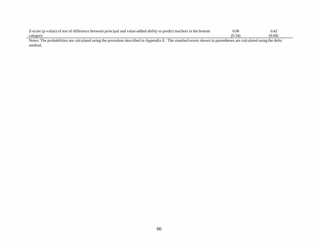
66

Z-score (p-value) of test of difference between principal and value-added ability to predict teachers in the bottom category

0.96 (0.34)

0.42 (0.68)

Notes: The probabilities are calculated using the procedure described in Appendix E. The standard errors shown in parentheses are calculated using the delta method.

67

TABLE VIII

THE ASSOCIATION BETWEEN PRINCIPAL RATINGS AND PRIOR VALUE-ADDED ON FUTURE ACHIEVEMENT SCORES Dependent Variable = 2003 Achievement Score

Readin

g Math

Independent Variables (1) (2) (3) (4) (5) (6) (7) (8) (9) (10) (11) (12)

Top principal group 0.174 (0.044)

0.154 (0.070)

Bottom principal group -0.021 (0.054)

-0.098 (0.067)

Top value-added group 0.160 (0.040)

0.207 (0.068)

Bottom value-added group -0.080 (0.045)

-0.148 (0.071)

Top group: value-added & principals

0.158 (0.038)

0.232 (0.062)

Bottom group: value-added & principals

-0.072 (0.046)

-0.128 (0.069)

Above median according to principal

0.125 (0.046)

0.028 (0.064)

Below median according to principal

0.034 (0.045)

-0.173 (0.058)

Above median according to value-added

0.122 (0.039)

0.169 (0.058)

Below median according to value-added

-0.080 (0.042)

-0.193 (0.071)

Above median according to value-added and principal

0.075 (0.040)

0.167 (0.060)

Below median according to value-added and principal

-0.106 (0.044)

-0.196 (0.067)

Notes: The specifications in columns 1-6 include 160 teachers and 3,834 students. The samples in columns 7-12 include 117 teachers and 2,582 students. All regressions include the following variables: male, special education status, free lunch eligibility, limited English proficiency, age, minority, fixed effects for grade and school, lagged math and reading score, class size, class-level average of student demographics and lagged achievement scores, an indicator for a mixed grade class and the following teacher demographics: male, untenured, experience in years, years known current principals, indicators for whether the teacher’s BA degree came from the local or other state college, an indicator for a MA (or higher) degree and an indicator for any additional teaching endorsements.

68

TABLE IX DO PRINCIPALS DISCRIMINATE?

Dependent Variable= Principal Rating of Teacher Ability to Raise Achievement

Independent Variables Reading Math EB estimate of teacher effectiveness -- 2.28**

(0.73) 1.85** (0.69) -- 1.35**

(0.36) 1.28** (0.34)

Male -0.55** (0.21)

-0.35* (0.21)

-0.44** (0.20)

-0.28 (0.21)

-0.46* (0.25)

-0.60** (0.23)

Untenured -0.61** (0.25)

-0.53** (0.25)

-0.56** (0.23)

-0.58** (0.25)

-0.61** (0.28)

-0.60** (0.27)

Years of Experience -0.01 (0.01)

-0.01 (0.01)

-0.01 (0.01)

-0.01 (0.01)

0.00 (0.01)

0.01 (0.01)

Grade 2-4 0.17 (0.15)

0.41** (0.17)

0.32** (0.16)

-0.03 (0.15)

0.14 (0.20)

0.02 (0.20)

Years known principal -0.02 (0.03)

-0.02 (0.03)

-0.03 (0.03)

0.00 (0.03)

-0.09* (0.04)

-0.07* (0.04)

BA Degree at in state (but not local) college

0.30 (0.25)

0.19 (0.24)

0.02 (0.22)

0.67** (0.25)

0.48* (0.29)

0.30 (0.27)

BA Degree at out of state college

0.33 (0.32)

0.31 (0.32)

0.27 (0.30)

-0.06 (0.33)

-0.07 (0.37)

-0.11 (0.34)

MA Degree -0.05 (0.20)

-0.25 (0.20)

-0.20 (0.19)

0.33 (0.20)

0.23 (0.22)

0.20 (0.20)

Additional endorsements 0.19 (0.19)

0.13 (0.19)

0.16 (0.18)

0.15 (0.19)

0.09 (0.21)

0.09 (0.19)

Relationship with administration 0.32**

(0.07) 0.32** (0.07)

School Fixed Effects Yes Yes Yes Yes Yes Yes R-Squared 0.14 0.19 0.29 0.14 0.18 0.29 Observations 202 202 202 151 151 151 Notes: Observations with missing teacher background data are set to zero and missing data indicators are included. All models also include school fixed effects. The EB estimates incorporate information on observed value-added as well as all of the other variables shown in this table. Standard errors are included in parenthesis. ** = significant at the 5 percent level; * = significant at the 10 percent level.

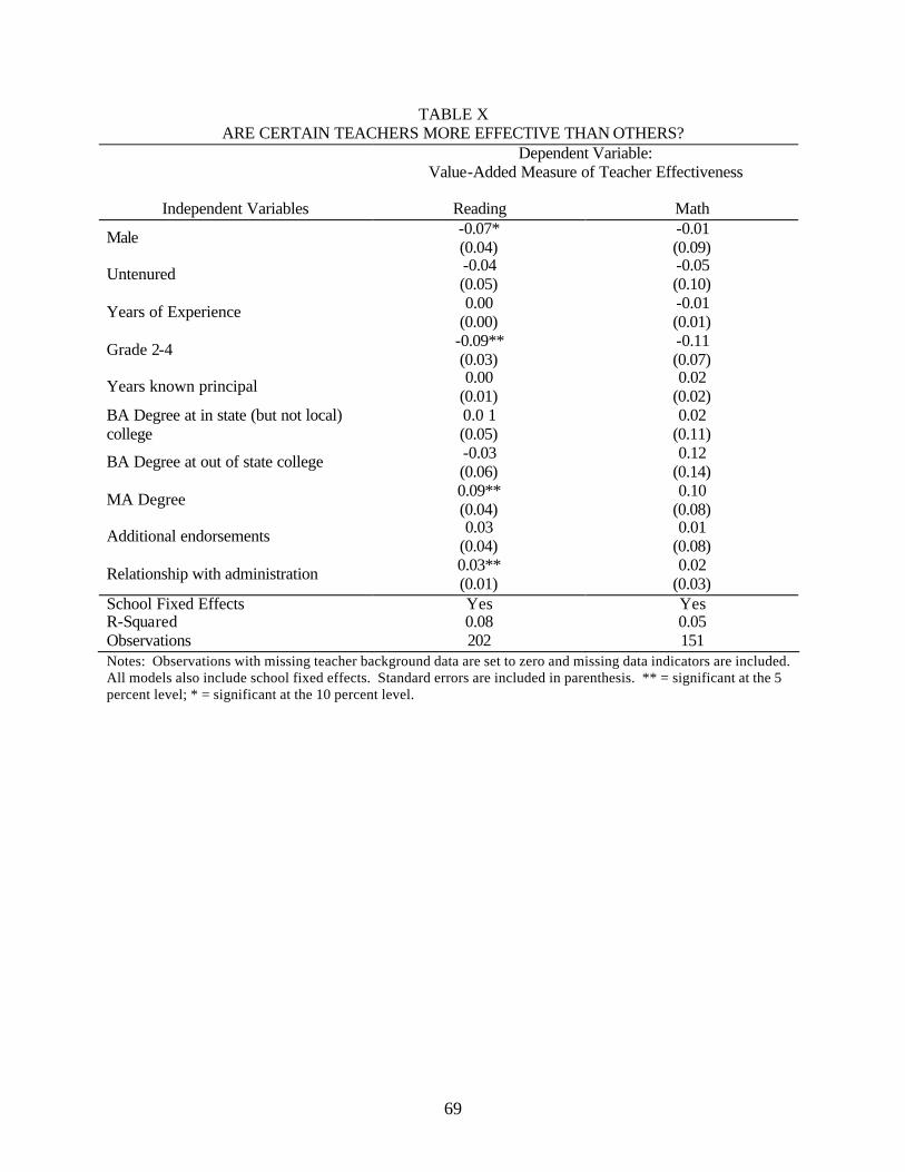
69

TABLE X ARE CERTAIN TEACHERS MORE EFFECTIVE THAN OTHERS?

Dependent Variable: Value-Added Measure of Teacher Effectiveness

Independent Variables Reading Math

Male -0.07* (0.04)

-0.01 (0.09)

Untenured -0.04 (0.05)

-0.05 (0.10)

Years of Experience 0.00 (0.00)

-0.01 (0.01)

Grade 2-4 -0.09** (0.03)

-0.11 (0.07)

Years known principal 0.00 (0.01)

0.02 (0.02)

BA Degree at in state (but not local) college

0.0 1 (0.05)

0.02 (0.11)

BA Degree at out of state college -0.03 (0.06)

0.12 (0.14)

MA Degree 0.09** (0.04)

0.10 (0.08)

Additional endorsements 0.03 (0.04)

0.01 (0.08)

Relationship with administration 0.03** (0.01)

0.02 (0.03)

School Fixed Effects Yes Yes R-Squared 0.08 0.05 Observations 202 151 Notes: Observations with missing teacher background data are set to zero and missing data indicators are included. All models also include school fixed effects. Standard errors are included in parenthesis. ** = significant at the 5 percent level; * = significant at the 10 percent level.

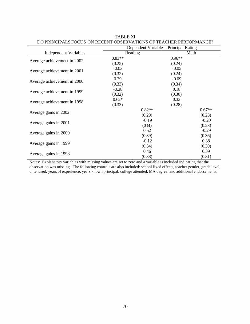
70

TABLE XI

DO PRINCIPALS FOCUS ON RECENT OBSERVATIONS OF TEACHER PERFORMANCE? Dependent Variable = Principal Rating

Independent Variables Reading Math

Average achievement in 2002 0.83** (0.25) 0.96**

(0.24)

Average achievement in 2001 -0.03 (0.32) -0.05

(0.24)

Average achievement in 2000 0.29 (0.33) -0.09

(0.34)

Average achievement in 1999 -0.28 (0.32) 0.18

(0.30)

Average achievement in 1998 0.62* (0.33) 0.32

(0.28)

Average gains in 2002 0.82** (0.29) 0.67**

(0.23)

Average gains in 2001 -0.19 (034) -0.20

(0.23)

Average gains in 2000 0.52 (0.39) -0.29

(0.36)

Average gains in 1999 -0.12 (0.34) 0.38

(0.30)

Average gains in 1998 0.46 (0.38) 0.39

(0.31) Notes: Explanatory variables with missing values are set to zero and a variable is included indicating that the observation was missing. The following controls are also included: school fixed effects, teacher gender, grade level, untenured, years of experience, years known principal, college attended, MA degree, and additional endorsements.

71

TABLE XII HOW DOES THE VARIANCE OF PRINCIPAL RATINGS CHANGE

WITH THE INFORMATION AVAILABLE TO THE PRINCIPAL?

Dependent Variable = Estimated Variance of Principal Rating

(1) (2) (3) (4) (5) Reading

Teacher Experience 0.004 (0.010)

0.010 (0.043)

Teacher Experience Squared -0.000 (0.002)

Years Principal Has Been with Teacher -0.008 (0.029)

0.019 (0.090)

Years Principal Has Been with Teacher Squared -0.002

(0.007)

Principal’s Confidence in Ability to Rate Math or Reading -0.277*

(0.153)

F-Statistic of Joint Significance 0.10 [p=0.90] 0.08

[p=0.93]

Observations 202 202 202 202 12 Math

Teacher Experience 0.005 (0.009)

0.036 (0.038)

Teacher Experience Squared -0.001 (0.001)

Years Principal Has Been with Teacher 0.027 (0.032)

0.002 (0.078)

Years Principal Has Been with Teacher Squared 0.002

(0.006)

Principal’s Confidence in Ability to Rate Math or Reading -0.060

(0.184)

F-Statistic of Joint Significance 0.46 [p=0.63] 0.36

[p=0.70]

Observations 202 202 202 202 12 Notes: For specifications 1 to 4, the dependent variable in these specifications is the squared residual of a regression of the principal’s reading or math rating on the teacher’s experience and experience squared. For specification 5, the dependent variable is the sample variance of a principal’s unadjusted reading or math rating on a linear scale of how confident the principal is in her ability to rank teachers. Specifications 1-4 are estimated on a sample of teachers (n=202) while specification 5 is estimated on a sample of principals (n=13). * Indicates significance at a 10 percent level.

72

TABLE XIII

DOES THE RELATIONSHIP BETWEEN THE ESTIMATED VALUE-ADDED AND PRINCIPAL RATING VARY WITH THE INFORMATION AVAILABLE TO THE PRINCIPAL?

Dependent Variable = Estimated Value-Added in Reading or Math

(1) (2) (3) Reading

Reading Rating 0.003 (0.021)

0.021 (0.022)

-0.031 (0.083)

Reading Rating*Years of Experience 0.003** (0.001)

Years of Experience -0.001 (0.001)

Reading Rating*Years Principal Has Been with Teacher 0.005*

(0.004)

Years Principal Has Been with Teacher -0.001 (0.004)

Reading Rating*Principal Confidence in Reading Rating 0.015

(0.017)

Principal Confidence in Reading 0.000 (0.02)

Observations 202 202 202 Math

Math Rating 0.032 (0.046)

0.092** (0.041)

-0.023 (0.131)

Math Rating*Years of Experience 0.004* (0.003)

Years of Experience -0.000 (0.003)

Math Rating*Years Principal Has Been with Teacher 0.000

(0.006)

Years Principal Has Been with Teacher 0.004 (0.007)

Math Rating*Principal Confidence in Reading Rating 0.025

(0.029)

Principal Confidence in Reading Rating 0.001 (0.028)

Observations 151 151 140 Notes: In this table, we show the coefficient from the regression of estimated reading or math value-added on the principal’s rating and rating interacted with proxies of the quality of the principal’s signal. **Indicates that the coefficient is significant at the 5 percent level in a one-sided test that the coefficient is greater than zero. * Indicates significance at the 10 percent level for the same test.