An Introduction to Splines - Simon Fraser...
13
An Introduction to Splines Contents 1 Introduction 1 2 Linear Regression 1 2.1 Simple Regression and the Least Squares Method .......................... 1 2.2 Simple Linear Regression in R ..................................... 3 2.3 Polynomial Regression ......................................... 5 3 Smoothing Splines 7 3.1 Truncated Polynomial Basis ....................................... 7 3.2 B-spline basis .............................................. 10 3.3 Overfitting, Smoothness and Penalization ............................... 11 1 Introduction One of the fundamental concepts of statistical modelling is the almost omnipresent balance between bias and precision. Models that derive from strong assumptions about the nature of a system produce precise estimates, but the estimates will be biased if the assumptions are not correct. On the other hand, models that derive from weaker assumptions are less prone to bias, but the resulting estimates are less precise. Much of the effort in constructing statistical models entails finding assumptions that strike the proper balance. Regression methods are used to model changes in a response variable as a function of changes in a predictor variable (or several predictor variables). Standard regression methods belong to the family of parametric models, meaning that they involve strong (parametric) assumptions about the nature of the system being modelled. At the other end of the spectrum, non-parametric regression models are an attempt to make no assumptions at all. Between these extremes lie the semi-parametric methods, which offer a balance by employing very general assumptions: for example, that the relationship between the response and predictor is continuous, or smooth in some sense, without being restricted to a specific shape. Splines belong to the class of semi-parametric techniques. 2 Linear Regression We will begin be discussing the common methods of parametric regression – including simple linear regression, the method of least squares, and polynomial regression – and then introduce the fundamental concepts of spline smoothing. Throughout the session we will base our examples on daily temperatures recorded in Montreal from 1961 to 1996. This data is freely available in the fds library for the R software package (hereafter referred to as R ). 2.1 Simple Regression and the Least Squares Method Simple Linear Regression Figure 1 depicts the temperatures observed in Montreal daily from April 1 to June 31, 1961. Not surprisingly, the daily temperature shows a consistent, increasing trend over this time period with temperatures near 0C in the early spring and reaching above 20C at the start of this summer. To describe this 1
Transcript of An Introduction to Splines - Simon Fraser...

An Introduction to Splines
Contents
1 Introduction 1
2 Linear Regression 12.1 Simple Regression and the Least Squares Method . . . . . . . . . . . . . . . . . . . . . . . . . . 12.2 Simple Linear Regression in R . . . . . . . . . . . . . . . . . . . . . . . . . . . . . . . . . . . . . 32.3 Polynomial Regression . . . . . . . . . . . . . . . . . . . . . . . . . . . . . . . . . . . . . . . . . 5
3 Smoothing Splines 73.1 Truncated Polynomial Basis . . . . . . . . . . . . . . . . . . . . . . . . . . . . . . . . . . . . . . . 73.2 B-spline basis . . . . . . . . . . . . . . . . . . . . . . . . . . . . . . . . . . . . . . . . . . . . . . 103.3 Overfitting, Smoothness and Penalization . . . . . . . . . . . . . . . . . . . . . . . . . . . . . . . 11
1 Introduction
One of the fundamental concepts of statistical modelling is the almost omnipresent balance between bias andprecision. Models that derive from strong assumptions about the nature of a system produce precise estimates,but the estimates will be biased if the assumptions are not correct. On the other hand, models that derive fromweaker assumptions are less prone to bias, but the resulting estimates are less precise. Much of the effort inconstructing statistical models entails finding assumptions that strike the proper balance.
Regression methods are used to model changes in a response variable as a function of changes in a predictorvariable (or several predictor variables). Standard regression methods belong to the family of parametric models,meaning that they involve strong (parametric) assumptions about the nature of the system being modelled. Atthe other end of the spectrum, non-parametric regression models are an attempt to make no assumptions atall. Between these extremes lie the semi-parametric methods, which offer a balance by employing very generalassumptions: for example, that the relationship between the response and predictor is continuous, or smoothin some sense, without being restricted to a specific shape. Splines belong to the class of semi-parametrictechniques.
2 Linear Regression
We will begin be discussing the common methods of parametric regression – including simple linear regression,the method of least squares, and polynomial regression – and then introduce the fundamental concepts of splinesmoothing. Throughout the session we will base our examples on daily temperatures recorded in Montreal from1961 to 1996. This data is freely available in the fds library for the R software package (hereafter referred to asR ).
2.1 Simple Regression and the Least Squares Method
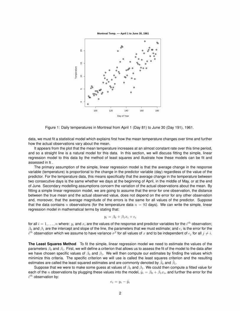
Simple Linear Regression Figure 1 depicts the temperatures observed in Montreal daily from April 1 to June31, 1961. Not surprisingly, the daily temperature shows a consistent, increasing trend over this time period withtemperatures near 0C in the early spring and reaching above 20C at the start of this summer. To describe this
1
●
●●●
●
●●
●●
●
●
●
●●
●
●●●
●●
●
●
●
●
●
●
●
●
●
●●
●
●
●
●
●
●
●
●
●
●●
●
●●
●
●
●
●●
●
●
●●
●
●
●
●
●
●
●
●
●
●
●●
●
●
●
●
●
●
●
●
●
●
●
●
●●
●
●
●
●●
●
●
●
●
●
●●
100 120 140 160 180
05
1015
20
Montreal Temp. −− April 1 to June 30, 1961
Day of Year
Tem
pera
ture
Figure 1: Daily temperatures in Montreal from April 1 (Day 81) to June 30 (Day 191), 1961.
data, we must fit a statistical model which explains first how the mean temperature changes over time and furtherhow the actual observations vary about the mean.
It appears from the plot that the mean temperature increases at an almost constant rate over this time period,and so a straight line is a natural model for this data. In this section, we will discuss fitting the simple, linearregression model to this data by the method of least squares and illustrate how these models can be fit andassessed in R .
The primary assumption of the simple, linear regression model is that the average change in the responsevariable (temperature) is proportional to the change in the predictor variable (day) regardless of the value of thepredictor. For the temperature data, this means specifically that the average change in the temperature betweentwo consecutive days is the same whether we days at the beginning of April, in the middle of May, or at the endof June. Secondary modelling assumptions concern the variation of the actual observations about the mean. Byfitting a simple linear regression model, we are going to assume that the error for one observation, the distancebetween the true mean and the actual observed value, does not depend on the error for any other observationand, moreover, that the average magnitude of the errors is the same for all values of the predictor. Supposethat the data contains n observations (for the temperature data n = 92 days). We can write the simple, linearregression model in mathematical terms by stating that:
yi = β0 + β1xi + εi
for all i = 1, . . . , n where: yi and xi are the values of the response and predictor variables for the ith observation;β0 and β1 are the intercept and slope of the line, the parameters that we must estimate; and εi is the error for theith observation which we assume to have variance σ2 for all values of x and to be independent of εj for all j 6= i.
The Least Squares Method To fit the simple, linear regression model we need to estimate the values of theparameters β0 and β1. First, we will define a criterion that allows us to assess the fit of the model to the data afterwe have chosen specific values of β0 and β1. We will then compute our estimates by finding the values whichminimize this criteria. The specific criterion we will use is called the least squares criterion and the resultingestimates are called the least squared estimates and are commonly denoted by β0 and β1.
Suppose that we were to make some guess at values of β0 and β1. We could then compute a fitted value foreach of the n observations by plugging these values into the model, yi = β0 + β1xi, and further the error for theith observation by:
ei = yi − yi
2
the difference between the observed and fitted value, called the residual. Intuitively, the values of β0 and β1 aregood if the fitted values are close to the observed values and the residuals are small. It will never be possible tomake all of the residuals equal to 0 (except in the unlikely case that the points actually lie along a straight line)so instead we will estimate β0 and β1 by making the average of the residuals as small as possible (actually, theaverage of the square of the residuals). The least squares fitting criterion is:
SS =∑
e2 =∑
(y − (β0 + β1x))2,
the sum of the squared residuals, and the least squares estimates are the values of β0 and β1 which minimizethis criterion. Although these estimates can be computed explicitly for the simple, linear regression model, this isnot true in general and we focus instead on how to fit this model in R .
2.2 Simple Linear Regression in R
Least Squares Fitting R Linear regression models can be fit in R using the lm function. Suppose that the valuesof the response, the observed temperatures, are stored in the vector y and values of the predictor, the days from80 to 191, in the vector x. The command to fit the linear regression model is simply: lm(y~x). Executing thiscommand in R returns the estimates of the two parameters which are: β0 = −15.4 and β1 = .2. This indicatesthat the mean temperature increases by .2C every day and that if the linear model applied to the data before April1 then the mean temperature on day 0 (December 31 of the previous year) would be -15.4C. As we will see, thisassumption is not justified so the interpretation of β0 is not so simple. Instead, it would be better to say that themean temperature on day 80, the first day of observation, is −15.4 + .2(80) = .6C.
The first argument of the lm function is a formula which specifies the structure of the regression model. Thetilde operator separates the response, on the left, from specification of the predictor variables, on the right. Bydefault, R includes an intercept in the structure of the model, so we don’t need to specify this explicitly. If we hadmultiple predictors of y, then we would list them all on the right hand side. For example, the formula y~x1 + x2defines y as a linear function of x1 and x2:
y = β0 + β1x1 + β1x2.
Again, we do not need to list the intercept in the predictors because it is included by default. There are severaloperators that can be used to define more complicated structures with multiple predictors. For example, themodel including the interaction term between the two variables can be written as x1 + x2 + x1:x2 or moresuccinctly as x1*x2. More information on defining formula can be obtained using the command help(formula).
Plotting the Fitted Curve The lm function actually produces much more output which can be accessed bystoring the results in a new variable, say lmfit: lmfit=lm(y~x,data). A full list of the output can be obtainedwith the command attributes(lmfit) and details for each component are provided in the help file accessed bythe command help(lm). One product of the function is the vector of fitted values for each observation, computedas:
yi = β0 + β1xi
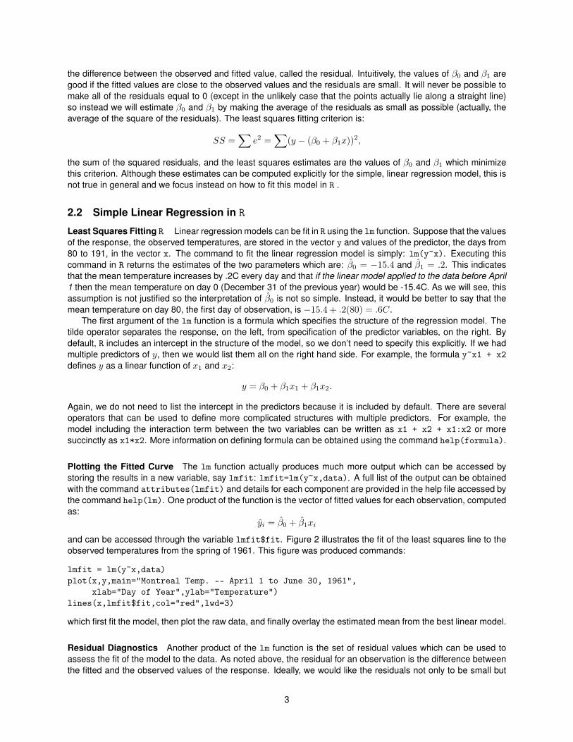
and can be accessed through the variable lmfit$fit. Figure 2 illustrates the fit of the least squares line to theobserved temperatures from the spring of 1961. This figure was produced commands:
lmfit = lm(y~x,data)plot(x,y,main="Montreal Temp. -- April 1 to June 30, 1961",
xlab="Day of Year",ylab="Temperature")lines(x,lmfit$fit,col="red",lwd=3)
which first fit the model, then plot the raw data, and finally overlay the estimated mean from the best linear model.
Residual Diagnostics Another product of the lm function is the set of residual values which can be used toassess the fit of the model to the data. As noted above, the residual for an observation is the difference betweenthe fitted and the observed values of the response. Ideally, we would like the residuals not only to be small but
3
●
●●●
●
●●
●●
●
●
●
●●
●
●●●
●●
●
●
●
●
●
●
●
●
●
●●
●
●
●
●
●
●
●
●
●
●●
●
●●
●
●
●
●●
●
●
●●
●
●
●
●
●
●
●
●
●
●
●●
●
●
●
●
●
●
●
●
●
●
●
●
●●
●
●
●
●●
●
●
●
●
●
●●
100 120 140 160 180
05
1015
20
Montreal Temp. −− April 1 to June 30, 1961
Day of Year
Tem
pera
ture
Figure 2: Daily temperatures in Montreal from April 1 (Day 81) to June 30 (Day 191), 1961: simple, linearregression model.
also to have the same size, on average, for all values of the response and the predictor. This can be assessedby constructing plots of the residuals versus x and y. If the model fits the data well, then both plots will show aneven scatter of the residuals about 0 with no discernible pattern. If there are regions in which the residuals areconsistently above or below 0 in either plot, then this indicates that the model has not properly captured the trendin the mean and that more structure is needed in the model. If the residuals in some regions are much largerthan in other regions, commonly visible as an overall funnel or football shape, then this indicates that the varianceof the errors is not constant.
Residual plots produced from the fit of the simple, linear regression model to the Montreal temperatures inthe spring of 1961 are shown in Figure 3. Both plots show a fairly good scatter of the residuals about 0, with theexception of the residuals for the observations from days 129, 133, 134, 135 and 164, which are much higher thanthose on the other days, and for the observations from days 146 and 150 which are much lower than those on theother days. These observations are outliers, meaning that their values are not explained properly by the model.It is possible that these values are unusually large because of a phenomenon that is not included in the model,like an unusually warm week that does not fit the slow warming trend. It is also possible that these observationsresult from error in the measuring device or in data transcription – perhaps the temperature on May 9 was not19.8C as recorded but in fact 9.8C, which would lie almost exactly on the fitted line. In practice, these outlierscan be removed if it is known that they resulted from errors in the data or else the model should be expanded toaccount for the unusual behaviour. This issue will not be explored further here.
Exercises
1. Montreal Temperature Data – April 1 to June 30, 1961Code for fitting the simple linear regression model to the Montreal temperature data from the spring of 1961is included in the file montreal_temp_1.R. Use this code to fit the model, plot the fitted line, and producethe residual plots.
2. Montreal Temperature Data – January 1 to December 31, 1961Repeat exercise 1 with the data from all of 1961 using the code in the file montreal_temp_2.R.
4

●
●
●●
●
●
●
●
●●
●
●
●
●
●
●●●
●●
●
●
●
●
●
●
●
●
●
●
●
●
●
●
●
●
●
●
●
●
●
●
●
●●
●
●
●
●●
●
●
●●●
●
●
●
●
●
●
●
●
●
●
●
●
●
●
●
●
●
●
●
●
●
●
●
●●
●
●
●
●●
●
●
●
●
●
●●
100 120 140 160 180
−10
−5
05
10
Day of Year
Res
idua
l
●
●
●●
●
●
●
●
●●
●
●
●
●
●
●●●
●●
●
●
●
●
●
●
●
●
●
●
●
●
●
●
●
●
●
●
●
●
●
●
●
●●
●
●
●
●●
●
●
●●●
●
●
●
●
●
●
●
●
●
●
●
●
●
●
●
●
●
●
●
●
●
●
●
●●
●
●
●
●●
●
●
●
●
●
●●
0 5 10 15 20
−10
−5
05
10
Temperature
Res
idua
lFigure 3: Residual daily temperatures in Montreal from April 1 (Day 81) to June 30 (Day 191), 1961 versus day(left) and temperature (right).
2.3 Polynomial Regression
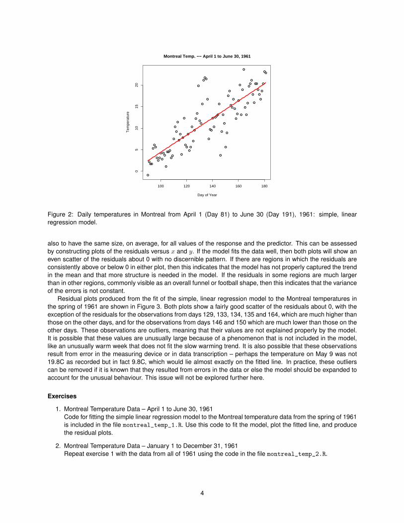
Polynomial Regression The assumption of linearity is often adequate for describing relationships over smallperiods of time, but not for modelling long term trends. This is clear in the case of the Montreal temperaturedata. Although the linear increase describes the changes in mean temperature well for the spring of 1961, thetrend over the entire year is clearly not linear. The mean temperature increases during the spring, plateaus inthe summer, and decreases again in the fall (After all, Montreal is in the northern hemisphere). The left panelof Figure 4 illustrates the best linear fit to the Montreal temperature data for all of 1961 and shows that themodel overestimates the mean temperature at the start of the year, underestimates in the middle of the year, andoverestimates again at the end of the year. This behaviour is also clear from the residual plot in the right panel.
One way that the new relationship can be modelled is by constructing the predictor as a polynomial in x: afunction that includes powers of x like the quadratic (x2), cubic (x3), and quartic (x4) terms . Suppose that wewish to model the response as a degree D polynomial in the predictor. The mathematical equation is:
y = β0 + β1x+ β2x2 + . . .+ βDx
D
or:
y = β0 +D∑
k=1
βdxd
using summation notation. Estimates of the coefficients β0, . . . , βD can again be found by minimizing the leastsquares criterion:
SS =n∑
i=1
e2i =n∑
i=1
(yi − yi)2
where ei is still the residual but the fitted value is now given by yi = β0 +∑D
k=1 βdxdi . As in the case of simple,
linear regression, explicit expressions for the least squares estimates do exist (using matrix notation) but we willinstead consider how to fit these models R .
The Design Matrix The Dth degree polynomial model can again be fit in R using the lm function. One wayto construct the polynomial would be to define new variables containing the values of x2, x3, . . . , xD and then
5
●●
●●
●
●
●●
●
●
●
●
●
●
●
●
●
●
●
●●
●
●
●
●●
●
●
●
●
●
●●
●
●●
●
●
●
●●
●
●●
●
●
●
●
●
●
●
●
●
●
●
●
●
●●
●
●
●
●
●
●●
●
●
●
●
●
●
●
●
●
●
●
●●
●
●
●
●●
●
●
●
●●
●
●●●
●●●
●●●●
●
●●
●
●●●
●●
●
●●
●
●
●
●
●
●
●●
●
●●
●
●
●
●●
●
●●
●
●●●
●
●
●●
●
●
●●●
●
●
●
●
●
●
●
●●
●●
●
●
●●
●
●
●
●
●
●
●
●
●●●
●
●
●●
●●●
●
●
●●
●●
●
●
●●●●●●●
●●
●●
●
●●●●●
●●
●
●
●
●
●●
●
●●
●
●●
●●●●●
●
●
●
●
●
●
●●
●
●
●●●
●
●●●
●●●
●
●
●
●
●
●
●
●
●
●●
●
●
●
●
●
●
●●
●
●
●
●●
●
●
●
●
●
●
●
●
●
●
●
●
●
●●
●
●
●
●
●
●
●
●●
●
●
●
●
●●
●●
●
●
●
●
●
●
●
●●
●●
●
●●
●
●
●
●
●
●●
●
●
●
●
●●
●
●
●●
●
●
●
●●
●●
●
●
●
●
●●
●
●
●
●●●
●
●
●
●
●●●
●
●●
●
●
●
●
●
●●
●
0 100 200 300
−20
−10
010
20
Montreal Temp. −− January 1 to December 31, 1961
Day of Year
Tem
pera
ture
●●
●●
●
●
●●
●
●
●
●
●
●
●
●
●
●
●
●●
●
●
●
●
●
●
●
●
●
●
●●
●
●●
●
●
●
●●
●
●●
●
●
●
●
●
●
●
●
●
●
●
●
●
●●
●
●
●
●
●
●●
●
●
●
●
●
●
●
●
●
●
●
●●
●
●
●
●●
●
●
●
●●
●
●●●
●●●
●●●●
●
●●
●
●●●
●●
●
●●
●
●
●
●
●
●
●●
●
●●
●
●
●
●●
●
●●
●
●●●
●
●
●●
●
●
●●●
●
●
●
●
●
●
●
●●
●●
●
●
●●
●
●
●
●
●
●
●
●
●●●
●
●
●●
●●●
●
●
●●
●●
●
●
●●●●●●●
●●
●●
●
●●●●●
●●
●
●
●
●
●●
●
●●
●
●●
●●●●●
●
●
●
●
●
●
●●
●
●
●●●
●
●●●
●●●
●
●
●
●
●
●
●
●
●
●●
●
●
●
●
●
●
●●
●
●
●
●●
●
●
●
●
●
●
●
●
●
●
●
●
●
●●
●
●
●
●
●
●
●
●●
●
●
●
●
●●
●●
●
●
●
●
●
●
●
●●
●●
●
●●
●
●
●
●
●
●●
●
●
●
●
●●
●
●
●●
●
●
●
●●
●●
●
●
●
●
●●
●
●
●
●●
●
●
●
●
●
●●●
●
●●
●
●
●
●
●
●●
●
0 100 200 300
−20
−10
010
20
Day of Year
Res
idua
lFigure 4: Daily temperatures in Montreal from January (Day 1) to December 31 (Day 365), 1961: fitted simple,linear regression model (left) and corresponding residuals versus day (right).
to list these values on the right hand side of the formula. However, a simpler way to do this is to construct adesign matrix which contains all of the values in a single object. In a multiple regression problem including nobservations and p predictor variables, the design matrix is the n × p matrix whose ith row contains the valuesof each of the predictor variables associated with the ith observation (alternatively, whose jth columns containsthe values for the jth predictor for each individual). For the degree D polynomial regression model, the ith rowof the design matrix will contain the values 1, xi, x
2i , . . . , x
Di . In total, there are in fact D + 1 predictor variables
and the 1 in the first entry represents the intercept term.
Constructing the Design Matrix in R The design matrix for the degree D polynomial regression model caneasily be constructed in R with the function outer. This function takes three arguments, two vectors and abinary operator (e.g., addition, subtraction, multiplication etc), and returns a matrix that is formed by applyingthe specified operator to each pair of elements from the two vectors. To construct the design matrix, we willsupply the vector of predictor values (x), the vector of exponents in the model (1, . . . , D), and the exponentiationoperator ^. The command is:
X = outer(x,1:D,"^")
and the linear model is then fit as:
lmfit = lm(y~X,data=data)
Note that the lm function includes the intercept term by default, so it is not necessary to put the leading 1 in thedesign matrix.
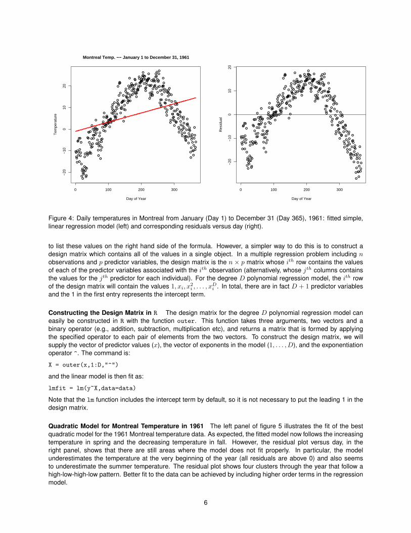
Quadratic Model for Montreal Temperature in 1961 The left panel of figure 5 illustrates the fit of the bestquadratic model for the 1961 Montreal temperature data. As expected, the fitted model now follows the increasingtemperature in spring and the decreasing temperature in fall. However, the residual plot versus day, in theright panel, shows that there are still areas where the model does not fit properly. In particular, the modelunderestimates the temperature at the very beginning of the year (all residuals are above 0) and also seemsto underestimate the summer temperature. The residual plot shows four clusters through the year that follow ahigh-low-high-low pattern. Better fit to the data can be achieved by including higher order terms in the regressionmodel.
6

●●
●●
●
●
●●
●
●
●
●
●
●
●
●
●
●
●
●●
●
●
●
●●
●
●
●
●
●
●●
●
●●
●
●
●
●●
●
●●
●
●
●
●
●
●
●
●
●
●
●
●
●
●●
●
●
●
●
●
●●
●
●
●
●
●
●
●
●
●
●
●
●●
●
●
●
●●
●
●
●
●●
●
●●●
●●●
●●●●
●
●●
●
●●●
●●
●
●●
●
●
●
●
●
●
●●
●
●●
●
●
●
●●
●
●●
●
●●●
●
●
●●
●
●
●●●
●
●
●
●
●
●
●
●●
●●
●
●
●●
●
●
●
●
●
●
●
●
●●●
●
●
●●
●●●
●
●
●●
●●
●
●
●●●●●●●
●●
●●
●
●●●●●
●●
●
●
●
●
●●
●
●●
●
●●
●●●●●
●
●
●
●
●
●
●●
●
●
●●●
●
●●●
●●●
●
●
●
●
●
●
●
●
●
●●
●
●
●
●
●
●
●●
●
●
●
●●
●
●
●
●
●
●
●
●
●
●
●
●
●
●●
●
●
●
●
●
●
●
●●
●
●
●
●
●●
●●
●
●
●
●
●
●
●
●●
●●
●
●●
●
●
●
●
●
●●
●
●
●
●
●●
●
●
●●
●
●
●
●●
●●
●
●
●
●
●●
●
●
●
●●●
●
●
●
●
●●●
●
●●
●
●
●
●
●
●●
●
0 100 200 300
−20
−10
010
20
Montreal Temp. −− January 1 to December 31, 1961
Day of Year
Tem
pera
ture
●
●
●
●
●
●
●●
●
●
●
●
●
●
●
●
●
●
●
●●
●
●
●
●
●
●
●
●
●
●
●●
●
●
●
●
●
●
●●
●
●●
●
●
●
●
●
●
●
●
●
●
●
●
●
●
●
●
●
●
●
●
●●
●
●
●
●
●
●
●
●
●
●
●
●
●
●
●
●
●●
●
●
●
●
●
●
●●●
●●●
●
●●
●
●
●●
●
●●●
●●
●
●
●
●
●
●
●
●
●
●●
●
●●
●
●
●
●
●
●
●●
●
●●●
●
●
●●
●
●
●●●
●
●
●
●
●
●
●
●
●
●●
●
●
●
●
●
●
●
●
●
●
●
●
●●●
●
●
●●
●
●
●
●
●
●●
●●
●
●
●
●●●●
●●
●
●
●●
●
●●●●●
●
●
●
●
●
●
●●
●
●
●
●
●
●
●●●●●
●
●
●
●
●
●
●
●
●
●
●
●●
●
●
●●
●●●
●
●
●
●
●
●
●
●
●
●●
●
●
●
●
●
●
●●
●
●
●
●●
●
●
●
●
●
●
●
●
●
●
●
●
●
●●
●
●
●
●
●
●
●
●
●
●
●
●
●
●●
●
●
●
●
●
●
●
●
●
●●
●●
●
●●
●
●
●
●
●
●●
●
●
●
●
●
●
●
●
●
●
●
●
●
●
●
●●
●
●
●
●
●●
●
●
●
●
●
●
●
●
●
●
●
●
●
●
●●
●
●
●
●
●
●
●
●
0 100 200 300
−15
−10
−5
05
1015
Day of Year
Res
idua
lFigure 5: Daily temperatures in Montreal from January 1 (Day 1) to December 31 (Day 365), 1961: fitted quadraticregression model (left) and corresponding residuals versus day (right).
Exercises
1. Montreal Temperature Data – January 1 to December 31, 1961Use the code in the file montreal_temp_3.R to fit polynomial regression models of varying degree to thedata for all of 1961. Models of different degree are constructed by changing the variable D (e.g., D=2produces a quadratic model and D=3 a cubic). What is the minimal degree required for the model to fitwell?
2. Montreal Temperature Data – January 1, 1961, to December 31, 1962Use the code in the file montreal_temp_4.R to repeat this exercise using the data recorded in both 1961and 1962.
3 Smoothing Splines
3.1 Truncated Polynomial Basis
Piecewise Polynomials Figure 6 shows the fit of an 8th degree polynomial to all of the data from 1961 and1962. The model does fit the mean temperature fairly well (except, perhaps, for an unusually cold period at theend of January, 1962) but is fairly complicated and difficult to interpret. Linear and quadratic models have simpleinterpretations – a linear model represents a system with a constant rate of change and a quadratic model asystem with a rate of change that increases or decreases at a fixed rate (the acceleration). Even a cubic modelcan be believed to represent some underlying process in the system – the acceleration changes at a constantrate. However, polynomials of higher degree are hard to interpret, and it is difficult to believe that the fittedequation actually represents the underlying behaviour in the system. What does the 8th degree polynomial sayabout the change in temperature in the spring of 1962, and how does this compare with the spring of the previousyear?
An alternative to increasing the degree of the fitted polynomial to account for curvature is to divide the range ofthe data into smaller pieces and fit simpler models to each of the subintervals. As seen in the previous sections,linear, quadratic or cubic polynomials are sufficient to fit small ranges of the data However, it seems reasonableto stipulate that the resulting function be continuous, without any jumps. Ideally, we would like the separate
7

●●
●●
●
●
●●
●●
●
●
●
●
●●
●
●
●
●●
●
●●
●●
●
●●
●●
●●
●
●●
●
●
●
●●
●
●●
●
●
●
●
●
●
●●
●
●●●
●●●
●
●
●
●
●
●●
●
●
●
●
●
●
●●
●
●
●
●●
●
●
●
●●
●
●
●
●●
●
●●●
●●●
●●●●●●●
●
●●●
●●
●
●●
●
●●
●
●
●
●●
●
●●
●
●
●
●●
●
●●
●
●●●
●
●
●●
●
●
●●●
●
●
●
●
●
●
●
●●
●●
●
●
●●
●
●
●
●
●
●
●
●
●●●
●
●
●●●●●
●
●
●●
●●
●
●
●●●●●●●
●●
●●●
●●●●●
●●●●
●
●
●●●
●●●
●●
●●●●●
●
●
●
●
●
●
●●
●
●
●●●
●
●●●
●●●
●
●●
●
●
●
●
●
●
●●
●●
●
●
●
●
●●
●
●
●
●●
●
●●
●●
●
●
●
●
●
●●
●
●●
●
●●
●
●
●
●
●●
●
●
●
●
●●
●●●
●
●
●
●●
●
●●
●●
●
●●
●
●
●●
●
●●
●
●
●
●●●
●●
●●
●
●
●
●●
●●
●
●
●
●
●●
●
●
●
●●●
●
●
●
●
●●●
●
●●
●
●
●
●
●
●●
●
●
●
●
●
●
●
●
●
●
●
●
●●
●
●
●
●
●
●●
●
●
●
●●
●●
●
●
●
●
●
●
●
●
●
●
●
●
●
●
●
●
●
●
●●
●
●
●
●
●
●
●
●
●
●
●
●
●
●●
●
●●
●●
●
●●
●●●
●●●
●
●
●
●
●
●
●
●●●
●
●
●
●
●
●●
●
●●●
●●
●●
●
●
●●●●●
●●
●●
●
●●
●
●
●
●
●
●●
●
●
●●
●●
●
●
●
●
●
●
●
●
●
●●
●●
●●
●
●
●●●
●
●●
●
●
●
●
●
●●●
●●
●
●
●
●
●●
●
●●
●
●
●●
●●
●
●
●
●●
●
●●
●
●●
●
●
●●●
●
●●●●
●
●●●●
●
●
●
●
●●
●●●●●
●
●
●
●
●
●
●●●●
●●●●●
●
●●
●
●●
●
●
●
●●●●
●
●●
●●●
●
●
●●●
●
●●
●
●
●
●●●
●
●●●●●
●
●●●●
●●●
●●
●
●●
●●●
●
●
●●●
●
●
●
●
●
●●
●
●
●●
●●
●
●
●●●
●●●
●
●
●●●●
●●●●
●●
●●
●
●●
●●
●
●
●●
●
●
●
●●●●
●
●●●
●
●
●●●
●
●
●●
●
●
●
●
●
●●
●
●
●
●
●●
0 200 400 600
−20
−10
010
20
Montreal Temp. −− January 1 to December 31, 1962
Day of Year
Tem
pera
ture
●
●
●
●
●
●
●●
●
●
●
●
●
●
●
●
●
●
●
●●
●
●
●
●
●
●
●
●
●
●
●●
●
●
●
●
●
●
●●
●
●●
●
●
●
●
●
●
●
●
●
●
●
●
●
●●
●
●
●
●
●
●●
●
●
●
●
●
●
●
●
●
●
●
●
●
●
●
●
●●
●
●
●
●
●
●
●●●
●●●
●
●●
●
●
●●
●
●●●
●●
●
●
●
●
●
●
●
●
●
●●
●
●●
●
●
●
●
●
●
●
●
●
●●●
●
●
●●
●
●
●●●
●
●
●
●
●
●
●
●
●
●●
●
●
●
●
●
●
●
●
●
●
●
●
●●●
●
●
●●
●
●
●
●
●
●●
●●
●
●
●
●●●●
●●
●
●
●●
●
●●●●●
●
●
●
●
●
●
●●
●
●
●
●
●
●
●●●●●
●
●
●
●
●
●
●
●
●
●
●
●●
●
●
●●
●●●
●
●
●
●
●
●
●
●
●
●●
●
●
●
●
●
●
●●
●
●
●
●●
●
●
●
●
●
●
●
●
●
●
●
●
●
●●
●
●
●
●
●
●
●
●
●
●
●
●
●
●●
●●
●
●
●
●
●
●
●
●●
●●
●
●●
●
●
●
●
●
●●
●
●
●
●
●
●
●
●
●
●
●
●
●
●●
●●
●
●
●
●
●●
●
●
●
●
●
●
●
●
●
●
●
●
●
●
●●
●
●
●
●
●
●
●
●
●
●
●
●
●
●
●
●
●
●
●
●
●
●
●
●
●
●
●●
●
●
●
●
●
●●
●
●
●
●
●
●
●
●
●
●
●
●
●
●
●
●
●
●
●
●
●
●
●
●
●
●
●
●
●
●
●
●
●
●
●
●
●●
●●
●
●●
●●●
●
●●
●
●
●
●
●
●
●
●●●
●
●
●
●
●
●●
●
●
●
●
●●
●●
●
●
●●●●●
●●
●
●
●
●●
●
●
●
●
●
●
●
●
●
●
●
●
●
●
●
●
●
●
●
●
●
●
●●
●
●
●●
●
●
●●
●
●
●
●
●
●
●
●
●
●●
●
●●
●
●
●
●
●●
●
●
●
●
●
●
●
●●
●
●
●
●●
●
●●
●
●●
●
●
●●●
●
●
●●●
●
●●●●
●
●
●
●
●
●
●●
●●
●
●
●
●
●
●
●
●
●●●
●
●
●●
●
●
●●
●
●
●
●
●
●
●●●
●
●
●
●
●
●●
●
●
●●●
●
●
●
●
●
●
●●●
●
●●
●
●
●
●
●●●●
●
●●
●●
●
●
●
●
●●
●
●
●●●
●
●
●
●
●
●●
●
●
●
●
●●
●
●
●●
●
●●
●
●
●
●●●●
●●
●●
●
●
●
●
●
●●
●●
●
●
●●
●
●
●
●●●●
●
●
●●
●
●
●
●●
●
●
●
●
●
●
●
●
●
●●
●
●
●
●
●●
0 200 400 600
−15
−10
−5
05
10
Day of Year
Res
idua
lFigure 6: Daily temperatures in Montreal from January 1, 1961 (Day 1), to December 31, 1962 (Day 730): fitted8th degree polynomial regression model (left) and corresponding residuals versus day (right).
polynomial pieces to connect at the boundaries of the intervals, and, perhaps, to produce a smooth curve overthe entire range of the data (whatever we may mean by smooth). This is exactly what a smoothing splines does.
Linear Splines The simplest spline (a spline of degree 1) is formed by connecting linear segments. Figure 7illustrates the fit of a linear spline to the Montreal temperature data for 1961 and 1962. The range of the data hasbeen divided into 10 subintervals of 73 days each and the fitted function is linear over each of the subintervals.The slope of the line is allowed to change between intervals, but the segments meet exactly at the intervalboundaries. In spline terminology, the dividing points are called the knots of the spline. To divide the range into10 subintervals requires 9 knots, and these are indicated by the red points in the figure. Mathematically, theequation for the linear spline is:
y = β0 + β1x+9∑
k=1
bk(x− ξk)+
where ξ1 = 73, ξ2 = 146, . . . , ξ9 = 637 are the knots of the spline. The function (x− ξ)+ is defined as:
(x− ξ)+ ={
0 x < ξx− ξ x > ξ
so that its value only affects the fit of the spline to the right of ξ. This is how the slope of the fitted functionchanges at each knot. For values of x left of the first knot the fitted function is simply y = β0 + β1x. Between thefirst and second knot the fitted function is y = β0 + β1x+ b1(x− ξ1) = (β0 − b1ξ1) + (β1 + b1)x. The result is anew linear segment which meets with the first segment at ξ1, but has a slope of β1 + b1. In general, the slope ofthe line between the kth and k + 1st knot is β1 + b1 + . . .+ bk−1.
The values of the parameters, including both β0 and β1 and the new parameters b1, . . . , b9, can once again beestimated by minimizing the least squares criterion and fit in R using the lm function. Note that the fitted functionrequires 11 parameters, so in some sense it is more complicated than the 8th degree polynomial which onlyrequired 9 parameters. However, the equation at any single point is much simpler and the fitted curve is mucheasier to interpret. The slope of the linear segment over the spring of 1961 is .24C/day and the slope over thespring of 1962 is .32. This suggests that the temperature rose faster in the spring of 162 than in 1961.
8
●●
●●
●
●
●●
●●
●
●
●
●
●●
●
●
●
●●
●
●●
●●
●
●●
●●
●●
●
●●
●
●
●
●●
●
●●
●
●
●
●
●
●
●●
●
●●●
●●●
●
●
●
●
●
●●
●
●
●
●
●
●
●●
●
●
●
●●
●
●
●
●●
●
●
●
●●
●
●●●
●●●
●●●●●●●
●
●●●
●●
●
●●
●
●●
●
●
●
●●
●
●●
●
●
●
●●
●
●●
●
●●●
●
●
●●
●
●
●●●
●
●
●
●
●
●
●
●●
●●
●
●
●●
●
●
●
●
●
●
●
●
●●●
●
●
●●●●●
●
●
●●
●●
●
●
●●●●●●●
●●
●●●
●●●●●
●●●●
●
●
●●●
●●●
●●
●●●●●
●
●
●
●
●
●
●●
●
●
●●●
●
●●●
●●●
●
●●
●
●
●
●
●
●
●●
●●
●
●
●
●
●●
●
●
●
●●
●
●●
●●
●
●
●
●
●
●●
●
●●
●
●●
●
●
●
●
●●
●
●
●
●
●●
●●●
●
●
●
●●
●
●●
●●
●
●●
●
●
●●
●
●●
●
●
●
●●●
●●
●●
●
●
●
●●
●●
●
●
●
●
●●
●
●
●
●●●
●
●
●
●
●●●
●
●●
●
●
●
●
●
●●
●
●
●
●
●
●
●
●
●
●
●
●
●●
●
●
●
●
●
●●
●
●
●
●●
●●
●
●
●
●
●
●
●
●
●
●
●
●
●
●
●
●
●
●
●●
●
●
●
●
●
●
●
●
●
●
●
●
●
●●
●
●●
●●
●
●●
●●●
●●●
●
●
●
●
●
●
●
●●●
●
●
●
●
●
●●
●
●●●
●●
●●
●
●
●●●●●
●●
●●
●
●●
●
●
●
●
●
●●
●
●
●●
●●
●
●
●
●
●
●
●
●
●
●●
●●
●●
●
●
●●●
●
●●
●
●
●
●
●
●●●
●●
●
●
●
●
●●
●
●●
●
●
●●
●●
●
●
●
●●
●
●●
●
●●
●
●
●●●
●
●●●●
●
●●●●
●
●
●
●
●●
●●●●●
●
●
●
●
●
●
●●●●
●●●●●
●
●●
●
●●
●
●
●
●●●●
●
●●
●●●
●
●
●●●
●
●●
●
●
●
●●●
●
●●●●●
●
●●●●
●●●
●●
●
●●
●●●
●
●
●●●
●
●
●
●
●
●●
●
●
●●
●●
●
●
●●●
●●●
●
●
●●●●
●●●●
●●
●●
●
●●
●●
●
●
●●
●
●
●
●●●●
●
●●●
●
●
●●●
●
●
●●
●
●
●
●
●
●●
●
●
●
●
●●
0 200 400 600
−20
−10
010
20
Montreal Temp. −− January 1 to December 31, 1962
Day of Year
Tem
pera
ture
●
●
●
●
●
●
●
●
●
●
●
●
●
●
●
●
●
●
●
●
●
●
●
●
●
●
●
●●
●●
●
●
●●
●
●
●
●
●
●
●
●
●
●
●
●●
●
●
●
●
●
●
●
●
●
●
●●
●
●
●
●
●
●
●●
●
●●
●
●
●
●
●
●
●
●
●
●
●
●
●
●●
●
●
●
●
●
●●
●
●
●
●
●
●
●
●
●
●
●
●
●
●
●
●
●●
●
●
●
●
●
●
●●●
●●●
●
●●
●
●
●●
●
●●●
●●
●
●
●
●
●
●
●
●
●
●●
●
●●
●
●
●
●
●
●
●
●
●
●●●
●
●
●●
●
●
●●●
●
●
●
●
●
●
●
●
●
●●
●
●
●
●
●
●
●
●
●
●
●
●
●●●
●
●
●●
●
●
●
●
●
●●
●●
●
●
●
●●●●
●●
●
●
●●
●
●●●●●
●●
●
●
●
●
●●
●
●
●
●
●
●
●●●●●
●
●
●
●
●
●
●
●
●
●
●
●●
●
●
●●
●●●
●
●
●
●
●
●
●
●
●
●●
●
●
●
●
●
●
●●
●
●
●
●●
●
●
●
●
●
●
●
●
●
●
●
●
●
●●
●
●
●
●
●
●
●
●
●
●
●
●
●
●●
●●
●
●
●
●
●
●
●
●●
●●
●
●●
●
●
●
●
●
●●
●
●
●
●
●●
●
●
●
●
●
●
●
●
●
●●
●
●
●
●
●●
●
●
●
●
●
●
●
●
●
●
●
●
●
●
●●
●
●
●
●
●
●
●
●
●
●
●
●
●
●
●
●
●
●
●
●
●
●
●
●
●
●
●●
●
●
●
●
●
●
●
●
●
●
●
●
●
●
●
●
●
●
●
●
●
●
●
●
●
●
●
●
●
●
●
●
●
●
●
●
●
●
●
●
●
●
●
●●
●●
●
●●
●●●
●
●●
●
●
●
●
●
●
●
●●●
●
●
●
●
●
●●
●
●
●
●
●●
●●
●
●
●●●●●
●●
●●
●
●●
●
●
●
●
●
●
●
●
●
●●
●
●
●
●
●
●
●
●
●
●
●
●●
●
●
●●
●
●
●●
●
●
●
●
●
●
●
●
●
●●
●
●●
●
●
●
●
●●
●
●
●
●
●
●
●
●●
●
●
●
●●
●
●●
●
●●
●
●
●●●
●
●
●●●
●
●
●●●
●
●
●
●
●
●
●●
●●
●
●
●
●
●
●
●
●
●●●
●
●
●●
●
●
●●
●
●
●
●
●
●
●●●
●
●
●
●
●
●●
●
●
●●●
●
●
●
●
●
●
●●●
●
●●
●
●
●
●
●●●●
●
●●
●●
●
●
●
●
●●
●
●
●●●
●
●
●
●
●
●●
●
●
●
●
●●
●
●
●●
●
●●
●
●
●
●●●●
●●
●●
●
●
●
●
●
●●
●●
●
●
●●
●
●
●
●●●●
●
●
●●
●
●
●
●●
●
●
●
●
●
●
●
●
●
●
●
●
●
●
●
●●
0 200 400 600
−15
−10
−5
05
10
Day of Year
Res
idua
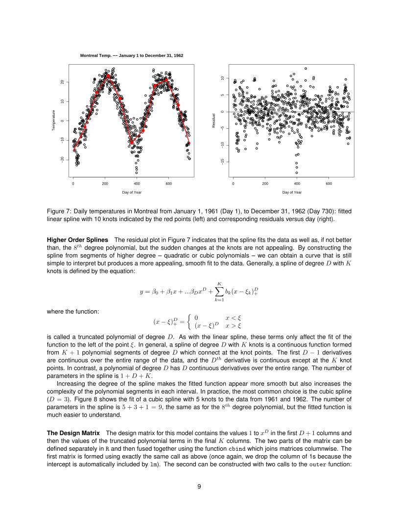
lFigure 7: Daily temperatures in Montreal from January 1, 1961 (Day 1), to December 31, 1962 (Day 730): fittedlinear spline with 10 knots indicated by the red points (left) and corresponding residuals versus day (right).
Higher Order Splines The residual plot in Figure 7 indicates that the spline fits the data as well as, if not betterthan, the 8th degree polynomial, but the sudden changes at the knots are not appealing. By constructing thespline from segments of higher degree – quadratic or cubic polynomials – we can obtain a curve that is stillsimple to interpret but produces a more appealing, smooth fit to the data. Generally, a spline of degree D with Kknots is defined by the equation:
y = β0 + β1x+ ...βDxD +
K∑k=1
bk(x− ξk)D+
where the function:
(x− ξ)D+ =
{0 x < ξ(x− ξ)D x > ξ
is called a truncated polynomial of degree D. As with the linear spline, these terms only affect the fit of thefunction to the left of the point ξ. In general, a spline of degree D with K knots is a continuous function formedfrom K + 1 polynomial segments of degree D which connect at the knot points. The first D − 1 derivativesare continuous over the entire range of the data, and the Dth derivative is continuous except at the K knotpoints. In contrast, a polynomial of degree D has D continuous derivatives over the entire range. The number ofparameters in the spline is 1 +D +K.
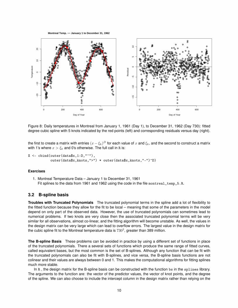
Increasing the degree of the spline makes the fitted function appear more smooth but also increases thecomplexity of the polynomial segments in each interval. In practice, the most common choice is the cubic spline(D = 3). Figure 8 shows the fit of a cubic spline with 5 knots to the data from 1961 and 1962. The number ofparameters in the spline is 5 + 3 + 1 = 9, the same as for the 8th degree polynomial, but the fitted function ismuch easier to understand.
The Design Matrix The design matrix for this model contains the values 1 to xD in the first D+ 1 columns andthen the values of the truncated polynomial terms in the final K columns. The two parts of the matrix can bedefined separately in R and then fused together using the function cbind which joins matrices columnwise. Thefirst matrix is formed using exactly the same call as above (once again, we drop the column of 1s because theintercept is automatically included by lm). The second can be constructed with two calls to the outer function:
9
●●
●●
●
●
●●
●●
●
●
●
●
●●
●
●
●
●●
●
●●
●●
●
●●
●●
●●
●
●●
●
●
●
●●
●
●●
●
●
●
●
●
●
●●
●
●●●
●●●
●
●
●
●
●
●●
●
●
●
●
●
●
●●
●
●
●
●●
●
●
●
●●
●
●
●
●●
●
●●●
●●●
●●●●●●●
●
●●●
●●
●
●●
●
●●
●
●
●
●●
●
●●
●
●
●
●●
●
●●
●
●●●
●
●
●●
●
●
●●●
●
●
●
●
●
●
●
●●
●●
●
●
●●
●
●
●
●
●
●
●
●
●●●
●
●
●●●●●
●
●
●●
●●
●
●
●●●●●●●
●●
●●●
●●●●●
●●●●
●
●
●●●
●●●
●●
●●●●●
●
●
●
●
●
●
●●
●
●
●●●
●
●●●
●●●
●
●●
●
●
●
●
●
●
●●
●●
●
●
●
●
●●
●
●
●
●●
●
●●
●●
●
●
●
●
●
●●
●
●●
●
●●
●
●
●
●
●●
●
●
●
●
●●
●●●
●
●
●
●●
●
●●
●●
●
●●
●
●
●●
●
●●
●
●
●
●●●
●●
●●
●
●
●
●●
●●
●
●
●
●
●●
●
●
●
●●●
●
●
●
●
●●●
●
●●
●
●
●
●
●
●●
●
●
●
●
●
●
●
●
●
●
●
●
●●
●
●
●
●
●
●●
●
●
●
●●
●●
●
●
●
●
●
●
●
●
●
●
●
●
●
●
●
●
●
●
●●
●
●
●
●
●
●
●
●
●
●
●
●
●
●●
●
●●
●●
●
●●
●●●
●●●
●
●
●
●
●
●
●
●●●
●
●
●
●
●
●●
●
●●●
●●
●●
●
●
●●●●●
●●
●●
●
●●
●
●
●
●
●
●●
●
●
●●
●●
●
●
●
●
●
●
●
●
●
●●
●●
●●
●
●
●●●
●
●●
●
●
●
●
●
●●●
●●
●
●
●
●
●●
●
●●
●
●
●●
●●
●
●
●
●●
●
●●
●
●●
●
●
●●●
●
●●●●
●
●●●●
●
●
●
●
●●
●●●●●
●
●
●
●
●
●
●●●●
●●●●●
●
●●
●
●●
●
●
●
●●●●
●
●●
●●●
●
●
●●●
●
●●
●
●
●
●●●
●
●●●●●
●
●●●●
●●●
●●
●
●●
●●●
●
●
●●●
●
●
●
●
●
●●
●
●
●●
●●
●
●
●●●
●●●
●
●
●●●●
●●●●
●●
●●
●
●●
●●
●
●
●●
●
●
●
●●●●
●
●●●
●
●
●●●
●
●
●●
●
●
●
●
●
●●
●
●
●
●
●●
0 200 400 600
−20
−10
010
20
Montreal Temp. −− January 1 to December 31, 1962
Day of Year
Tem
pera
ture
●
●
●
●
●
●
●
●
●
●●
●●
●
●
●●
●
●
●
●
●
●
●
●
●
●
●
●●
●
●
●
●
●
●
●
●
●
●
●●
●
●
●
●
●
●
●●
●
●●
●
●
●
●
●
●
●
●
●
●
●
●
●
●●
●
●
●
●
●
●●
●
●
●
●
●
●
●
●
●
●
●
●
●
●
●
●
●●
●
●
●
●
●
●
●●●
●●●
●
●●
●
●
●●
●
●●●
●●
●
●
●
●
●
●
●
●
●
●●
●
●●
●
●
●
●
●
●
●
●
●
●●●
●
●
●●
●
●
●●●
●
●
●
●
●
●
●
●
●
●●
●
●
●
●
●
●
●
●
●
●
●
●
●●●
●
●
●●
●
●
●
●
●
●●
●●
●
●
●
●●●●
●●
●
●
●●
●
●●●●●
●
●
●
●
●
●
●●
●
●
●
●
●
●
●●●●●
●
●
●
●
●
●
●
●
●
●
●
●●
●
●
●●
●●●
●
●
●
●
●
●
●
●
●
●●
●
●
●
●
●
●
●●
●
●
●
●●
●
●
●
●
●
●
●
●
●
●
●
●
●
●●
●
●
●
●
●
●
●
●
●
●
●
●
●
●●
●●
●
●
●
●
●
●
●
●●
●●
●
●●
●
●
●
●
●
●●
●
●
●
●
●
●
●
●
●
●
●
●
●
●
●
●●
●
●
●
●
●●
●
●
●
●
●
●
●
●
●
●
●
●
●
●
●●
●
●
●
●
●
●
●
●
●
●
●
●
●
●
●
●
●
●
●
●
●
●
●
●
●
●
●●
●
●
●
●
●
●
●
●
●
●
●
●
●
●
●
●
●
●
●
●
●
●
●
●
●
●
●
●
●
●
●
●
●
●
●
●
●
●
●
●
●
●
●
●●
●
●
●
●●
●●●
●
●●
●
●
●
●
●
●
●
●●●
●
●
●
●
●
●●
●
●
●
●
●●
●●
●
●
●●●●●
●●
●
●
●
●●
●
●
●
●
●
●
●
●
●
●
●
●
●
●
●
●
●
●
●
●
●
●
●●
●
●
●●
●
●
●●
●
●
●
●
●
●
●
●
●
●●
●
●●
●
●
●
●
●●
●
●
●
●
●
●
●
●●
●
●
●
●●
●
●●
●
●●
●
●
●●●
●
●
●●●
●
●
●●●
●
●
●
●
●
●
●●
●●
●
●
●
●
●
●
●
●
●●●
●
●
●●
●
●
●●
●
●
●
●
●
●
●●●
●
●
●
●
●
●●
●
●
●●●
●
●
●
●
●
●
●●●
●
●●
●
●
●
●
●
●●
●
●
●●
●●
●
●
●
●
●●
●
●
●●●
●
●
●
●
●
●●
●
●
●
●
●●
●
●
●●
●
●●
●
●
●
●●●●
●●
●●
●
●
●
●
●
●●
●●
●
●
●●
●
●
●
●●●●
●
●
●●
●
●
●
●●
●
●
●
●
●
●
●
●
●
●
●
●
●
●
●
●●
0 200 400 600
−15
−10
−5
05
10
Day of Year
Res
idua
lFigure 8: Daily temperatures in Montreal from January 1, 1961 (Day 1), to December 31, 1962 (Day 730): fitteddegree cubic spline with 5 knots indicated by the red points (left) and corresponding residuals versus day (right).
the first to create a matrix with entries (x− ξk)D for each value of x and ξk, and the second to construct a matrixwith 1’s where x > ξk and 0’s otherwise. The full call in R is:
X <- cbind(outer(data$x,1:D,"^"),outer(data$x,knots,">") * outer(data$x,knots,"-")^D)
Exercises
1. Montreal Temperature Data – January 1 to December 31, 1961Fit splines to the data from 1961 and 1962 using the code in the file montreal_temp_5.R.
3.2 B-spline basis
Troubles with Truncated Polynomials The truncated polynomial terms in the spline add a lot of flexibility tothe fitted function because they allow for the fit to be local – meaning that some of the parameters in the modeldepend on only part of the observed data. However, the use of truncated polynomials can sometimes lead tonumerical problems. If two knots are very close then the associated truncated polynomial terms will be verysimilar for all observations, almost co-linear, and the fitting algorithm will become unstable. As well, the values inthe design matrix can be very large which can lead to overflow errors. The largest value in the design matrix forthe cubic spline fit to the Montreal temperature data is 7303, greater than 389 million.
The B-spline Basis These problems can be avoided in practice by using a different set of functions in placeof the truncated polynomials. There a several sets of functions which produce the same range of fitted curves,called equivalent bases, but the most common is the set of B-splines. Although any function that can be fit withthe truncated polynomials can also be fit with B-splines, and vice versa, the B-spline basis functions are notcolinear and their values are always between 0 and 1. This makes the computational algorithms for fitting splinesmuch more stable.
In R , the design matrix for the B-spline basis can be constructed with the function bs in the splines library.The arguments to the function are: the vector of the predictor values, the vector of knot points, and the degreeof the spline. We can also choose to include the intercept column in the design matrix rather than relying on the
10

lm function to automatically include this. To make things simpler in the next section, we will choose to include theintercept term in design matrix and then tell lm not to add the column of ones. The full call is:
X <- bs(data$x,knots=knots,degree=D,intercept=TRUE)lmfit <- lm(y~X-1,data=data)
where the first command constructs the design matrix and the second fits the model. The notation -1 in theregression formula tells lm that the intercept is included in the design matrix and so it does not need to be added.Figure 9 shows the fit of a B-spline of degree 3 with 5 equally spaced knots. The fit is exactly the same as the fitof the degree 3 truncated polynomial spline with 5 knots shown in Figure 8.
●●
●●
●
●
●●
●●
●
●
●
●
●●
●
●
●
●●
●
●●
●●
●
●●
●●
●●
●
●●
●
●
●
●●
●
●●
●
●
●
●
●
●
●●
●
●●●
●●●
●
●
●
●
●
●●
●
●
●
●
●
●
●●
●
●
●
●●
●
●
●
●●
●
●
●
●●
●
●●●
●●●
●●●●●●●
●
●●●
●●
●
●●
●
●●
●
●
●
●●
●
●●
●
●
●
●●
●
●●
●
●●●
●
●
●●
●
●
●●●
●
●
●
●
●
●
●
●●
●●
●
●
●●
●
●
●
●
●
●
●
●
●●●
●
●
●●●●●
●
●
●●
●●
●
●
●●●●●●●
●●
●●●
●●●●●
●●●●
●
●
●●●
●●●
●●
●●●●●
●
●
●
●
●
●
●●
●
●
●●●
●
●●●
●●●
●
●●
●
●
●
●
●
●
●●
●●
●
●
●
●
●●
●
●
●
●●
●
●●
●●
●
●
●
●
●
●●
●
●●
●
●●
●
●
●
●
●●
●
●
●
●
●●
●●●
●
●
●
●●
●
●●
●●
●
●●
●
●
●●
●
●●
●
●
●
●●●
●●
●●
●
●
●
●●
●●
●
●
●
●
●●
●
●
●
●●●
●
●
●
●
●●●
●
●●
●
●
●
●
●
●●
●
●
●
●
●
●
●
●
●
●
●
●
●●
●
●
●
●
●
●●
●
●
●
●●
●●
●
●
●
●
●
●
●
●
●
●
●
●
●
●
●
●
●
●
●●
●
●
●
●
●
●
●
●
●
●
●
●
●
●●
●
●●
●●
●
●●
●●●
●●●
●
●
●
●
●
●
●
●●●
●
●
●
●
●
●●
●
●●●
●●
●●
●
●
●●●●●
●●
●●
●
●●
●
●
●
●
●
●●
●
●
●●
●●
●
●
●
●
●
●
●
●
●
●●
●●
●●
●
●
●●●
●
●●
●
●
●
●
●
●●●
●●
●
●
●
●
●●
●
●●
●
●
●●
●●
●
●
●
●●
●
●●
●
●●
●
●
●●●
●
●●●●
●
●●●●
●
●
●
●
●●
●●●●●
●
●
●
●
●
●
●●●●
●●●●●
●
●●
●
●●
●
●
●
●●●●
●
●●
●●●
●
●
●●●
●
●●
●
●
●
●●●
●
●●●●●
●
●●●●
●●●
●●
●
●●
●●●
●
●
●●●
●
●
●
●
●
●●
●
●
●●
●●
●
●
●●●
●●●
●
●
●●●●
●●●●
●●
●●
●
●●
●●
●
●
●●
●
●
●
●●●●
●
●●●
●
●
●●●
●
●
●●
●
●
●
●
●
●●
●
●
●
●
●●
0 200 400 600
−20
−10
010
20
Montreal Temp. −− January 1, 1961, to December 31, 1962
Day of Year
Tem
pera
ture
●
●
●
●
●
●●
●●
●
●
●●
●
●
●
●
●
●
●
●
●
●
●
●●
●
●
●
●
●
●
●
●
●
●
●●
●
●
●
●
●
●
●●
●
●●
●
●
●
●
●
●
●
●
●
●
●
●
●
●●
●
●
●
●
●
●●
●
●
●
●
●
●
●
●
●
●
●
●
●
●
●
●
●●
●
●
●
●
●
●
●●●
●●●
●
●●
●
●
●●
●
●●●
●●
●
●
●
●
●
●
●
●
●
●●
●
●●
●
●
●
●
●
●
●
●
●
●●●
●
●
●●
●
●
●●●
●
●
●
●
●
●
●
●
●
●●
●
●
●
●
●
●
●
●
●
●
●
●
●●●
●
●
●●
●
●
●
●
●
●●
●●
●
●
●
●●●●
●●
●
●
●●
●
●●●●●
●
●
●
●
●
●
●●
●
●
●
●
●
●
●●●●●
●
●
●
●
●
●
●
●
●
●
●
●●
●
●
●●
●●●
●
●
●
●
●
●
●
●
●
●●
●
●
●
●
●
●
●●
●
●
●
●●
●
●
●
●
●
●
●
●
●
●
●
●
●
●●
●
●
●
●
●
●
●
●
●
●
●
●
●
●●
●●
●
●
●
●
●
●
●
●●
●●
●
●●
●
●
●
●
●
●●
●
●
●
●
●
●
●
●
●
●
●
●
●
●
●
●●
●
●
●
●
●●
●
●
●
●
●
●
●
●
●
●
●
●
●
●
●●
●
●
●
●
●
●
●
●
●
●
●
●
●
●
●
●
●
●
●
●
●
●
●
●
●
●
●●
●
●
●
●
●
●
●
●
●
●
●
●
●
●
●
●
●
●
●
●
●
●
●
●
●
●
●
●
●
●
●
●
●
●
●
●
●
●
●
●
●
●
●
●●
●
●
●
●●
●●●
●
●●
●
●
●
●
●
●
●
●●●
●
●
●
●
●
●●
●
●
●
●
●●
●●
●
●
●●●●●
●●
●
●
●
●●
●
●
●
●
●
●
●
●
●
●
●
●
●
●
●
●
●
●
●
●
●
●
●●
●
●
●●
●
●
●●
●
●
●
●
●
●
●
●
●
●●
●
●●
●
●
●
●
●●
●
●
●
●
●
●
●
●●
●
●
●
●●
●
●●
●
●●
●
●
●●●
●
●
●●●
●
●
●●●
●
●
●
●
●
●
●●
●●
●
●
●
●
●
●
●
●
●●●
●
●
●●
●
●
●●
●
●
●
●
●
●
●●●
●
●
●
●
●
●●
●
●
●●●
●
●
●
●
●
●
●●●
●
●●
●
●
●
●
●
●●
●
●
●●
●●
●
●
●
●
●●
●
●
●●●
●
●
●
●
●
●●
●
●
●
●
●●
●
●
●●
●
●●
●
●
●
●●●●
●●
●●
●
●
●
●
●
●●
●●
●
●
●●
●
●
●
●●●●
●
●
●●
●
●
●
●●
●
●
●
●
●
●
●
●
●
●
●
●
●
●
●
●●
0 200 400 600
−15
−10
−5
05
10
Day of Year
Res
idua
l
Figure 9: Daily temperatures in Montreal from January 1, 1961 (Day 1), to December 31, 1962 (Day 730): fittedB-spline of degree 3 with 5 knots indicated by the red points (left) and corresponding residuals versus day (right).
Exercises
1. Montreal Temperature Data – January 1 to December 31, 1961Fit a B-spline to the data from 1961 and 1962 using the code in the file montreal_temp_5.R. Increase thenumber of knots to see how this affects the fit of the curve. What happens when the number of knots isvery large, say K = 50?
3.3 Overfitting, Smoothness and Penalization
Overfitting and Smoothness The spline with 5 knots used in the previous section seems to fit the Montrealtemperature data very well. It shows a smooth change in the mean over the two year period and captures theimportant trends in temperature. When the number of knots is increased further the subintervals contain only afew points each and the polynomial segments begin to interpolate the data. Figure 10 shows the fit of a spline ofdegree 3 with 50 equally spaced knots. The new curve still captures the overall behaviour, but it is also pickingout a lot of the details in the data. We say that the model is overfit. In general, there is a balance between the fitand the smoothness of a spline. A spline with only a few knots will be very smooth but may not be able to adaptto the shape of the data. A spline with many knots can easily adapt to the shape of the data but may lead tooverfitting.
11

●●
●●
●
●
●●
●●
●
●
●
●
●●
●
●
●
●●
●
●●
●●
●
●●
●●
●●
●
●●
●
●
●
●●
●
●●
●
●
●
●
●
●
●●
●
●●●
●●●
●
●
●
●
●
●●
●
●
●
●
●
●
●●
●
●
●
●●
●
●
●
●●
●
●
●
●●
●
●●●
●●●
●●●●●●●
●
●●●
●●
●
●●
●
●●
●
●
●
●●
●
●●
●
●
●
●●
●
●●
●
●●●
●
●
●●
●
●
●●●
●
●
●
●
●
●
●
●●
●●
●
●
●●
●
●
●
●
●
●
●
●
●●●
●
●
●●●●●
●
●
●●
●●
●
●
●●●●●●●
●●
●●●
●●●●●
●●●●
●
●
●●●
●●●
●●
●●●●●
●
●
●
●
●
●
●●
●
●
●●●
●
●●●
●●●
●
●●
●
●
●
●
●
●
●●
●●
●
●
●
●
●●
●
●
●
●●
●
●●
●●
●
●
●
●
●
●●
●
●●
●
●●
●
●
●
●
●●
●
●
●
●
●●
●●●
●
●
●
●●
●
●●
●●
●
●●
●
●
●●
●
●●
●
●
●
●●●
●●
●●
●
●
●
●●
●●
●
●
●
●
●●
●
●
●
●●●
●
●
●
●
●●●
●
●●
●
●
●
●
●
●●
●
●
●
●
●
●
●
●
●
●
●
●
●●
●
●
●
●
●
●●
●
●
●
●●
●●
●
●
●
●
●
●
●
●
●
●
●
●
●
●
●
●
●
●
●●
●
●
●
●
●
●
●
●
●
●
●
●
●
●●
●
●●
●●
●
●●
●●●
●●●
●
●
●
●
●
●
●
●●●
●
●
●
●
●
●●
●
●●●
●●
●●
●
●
●●●●●
●●
●●
●
●●
●
●
●
●
●
●●
●
●
●●
●●
●
●
●
●
●
●
●
●
●
●●
●●
●●
●
●
●●●
●
●●
●
●
●
●
●
●●●
●●
●
●
●
●
●●
●
●●
●
●
●●
●●
●
●
●
●●
●
●●
●
●●
●
●
●●●
●
●●●●
●
●●●●
●
●
●
●
●●
●●●●●
●
●
●
●
●
●
●●●●
●●●●●
●
●●
●
●●
●
●
●
●●●●
●
●●
●●●
●
●
●●●
●
●●
●
●
●
●●●
●
●●●●●
●
●●●●
●●●
●●
●
●●
●●●
●
●
●●●
●
●
●
●
●
●●
●
●
●●
●●
●
●
●●●
●●●
●
●
●●●●
●●●●
●●
●●
●
●●
●●
●
●
●●
●
●
●
●●●●
●
●●●
●
●
●●●
●
●
●●
●
●
●
●
●
●●
●
●
●
●
●●
0 200 400 600
−20
−10
010
20
Montreal Temp. −− January 1, 1961, to December 31, 1962
Day of Year
Tem
pera
ture
●
●
●
●
●
●
●
●
●●
●
●●
●●
●
●
●
●
●
●
●
●●
●●●
●
●
●
●
●
●
●
●
●●●
●●
●●
●
●
●
●
●
●●
Figure 10: Daily temperatures in Montreal from January 1, 1961 (Day 1), to December 31, 1962 (Day 730): fittedcubic B-spline with 50 knots indicated by the red points.
Knot Selection versus Penalization One way to avoid overfitting is to vary the number of knots (and theirlocation) until we find an arrangement that allows the spline to properly adapt to the shape of the data. However,finding the optimal set of knots can be a very complicated procedure that requires very intensive computing. Analternative strategy is to always use many knots, but to control overfitting by limiting the amount between thesegments in neighbouring intervals. Recall that the slope of the the linear spline constructed from truncatedpolynomials is β1 to the left of the first knot and β1 + b1 to the right. The difference in the slope may be verysevere if b1 is allowed to vary at will, but if we restrict the value of b1 then the slope will change slightly and thefitted function will always be smooth.
Penalization for Truncated Polynomials To ensure that the fitted spline doesn’t overfit the data we can definea new fitting criterion that attempts to minimize both the residuals and the values of the parameters b1, . . . , bK .The new criterion is:
n∑i=1
(yi − yi)2 + λ
K∑k=1
b2k
and is called the penalized least squares criterion because the second sum penalizes the coefficients. Althoughlarger values of b1, . . . , bK may improve the fit, and decrease the sum of squared residuals, they will increasethe penalty term and so may not be preferred. The value λ is called the smoothing parameter and controls thebalance between smoothnes and fit. If λ is large, then the criterion weights the penalty more heavily so that largevalues of bk are severely penalized and the resulting spline is very smooth. If λ is small then the penalty term willhave little effect and the spline will come close to interpolating the data.
Penalization for the B-spline Basis A spline formed in the B-spline basis becomes smoother as the differ-ences between the coefficients get smaller, not as the values of the individual coefficients approach 0. Hence,smoothness and fit will be balanced by a fitting criterion that penalizes the differences between the coefficientsinstead of their absolute values. For technical reasons that won’t be explained here, it actually makes more senseto penalize the second differences (i.e., the differences of the differences) of the coefficients when working with
12
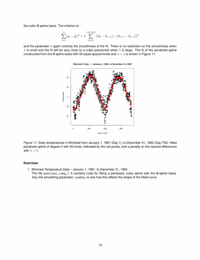
the cubic B-spline basis. The criterion is:
n∑i=1
(yi − yi)2 + λ
1+D+K∑k=3
((bk − bk−1)− (bk−1 − bk−2))2
and the parameter λ again controls the smoothness of the fit. There is no restriction on the smoothness whenλ is small and the fit will be very close to a cubic polynomial when λ is large. The fit of the penalized splineconstructed from the B-spline basis with 50 equal spaced knots and λ = 5 is shown in Figure 11.
●●
●●
●
●
●●
●●
●
●
●
●
●●
●
●
●
●●
●
●●
●●
●
●●
●●
●●
●
●●
●
●
●
●●
●
●●
●
●
●
●
●
●
●●
●
●●●
●●●
●
●
●
●
●
●●
●
●
●
●
●
●
●●
●
●
●
●●
●
●
●
●●
●
●
●
●●
●
●●●
●●●
●●●●●●●
●
●●●
●●
●
●●
●
●●
●
●
●
●●
●
●●
●
●
●
●●
●
●●
●
●●●
●
●
●●
●
●
●●●
●
●
●
●
●
●
●
●●
●●
●
●
●●
●
●
●
●
●
●
●
●
●●●
●
●
●●●●●
●
●
●●
●●
●
●
●●●●●●●
●●
●●●
●●●●●
●●●●
●
●
●●●
●●●
●●
●●●●●
●
●
●
●
●
●
●●
●
●
●●●
●
●●●
●●●
●
●●
●
●
●
●
●
●
●●
●●
●
●
●
●
●●
●
●
●
●●
●
●●
●●
●
●
●
●
●
●●
●
●●
●
●●
●
●
●
●
●●
●
●
●
●
●●
●●●
●
●
●
●●
●
●●
●●
●
●●
●
●
●●
●
●●
●
●
●
●●●
●●
●●
●
●
●
●●
●●
●
●
●
●
●●
●
●
●
●●●
●
●
●
●
●●●
●
●●
●
●
●
●
●
●●
●
●
●
●
●
●
●
●
●
●
●
●
●●
●
●
●
●
●
●●
●
●
●
●●
●●
●
●
●
●
●
●
●
●
●
●
●
●
●
●
●
●
●
●
●●
●
●
●
●
●
●
●
●
●
●
●
●
●
●●
●
●●
●●
●
●●
●●●
●●●
●
●
●
●
●
●
●
●●●
●
●
●
●
●
●●
●
●●●
●●
●●
●
●
●●●●●
●●
●●
●
●●
●
●
●
●
●
●●
●
●
●●
●●
●
●
●
●
●
●
●
●
●
●●
●●
●●
●
●
●●●
●
●●
●
●
●
●
●
●●●
●●
●
●
●
●
●●
●
●●
●
●
●●
●●
●
●
●
●●
●
●●
●
●●
●
●
●●●
●
●●●●
●
●●●●
●
●
●
●
●●
●●●●●
●
●
●
●
●
●
●●●●
●●●●●
●
●●
●
●●
●
●
●
●●●●
●
●●
●●●
●
●
●●●
●
●●
●
●
●
●●●
●
●●●●●
●
●●●●
●●●
●●
●
●●
●●●
●
●
●●●
●
●
●
●
●
●●
●
●
●●
●●
●
●
●●●
●●●
●
●
●●●●
●●●●
●●
●●
●
●●
●●
●
●
●●
●
●
●
●●●●
●
●●●
●
●
●●●
●
●
●●
●
●
●
●
●
●●
●
●
●
●
●●
0 200 400 600
−20
−10
010
20
Montreal Temp. −− January 1, 1961, to December 31, 1962
Day of Year
Tem
pera
ture
●●
●
●
●
●
●
●
●
●
●
●
●●●●●
●
●
●
●
●
●
●
●
●
●●
●
●
●
●
●
●
●
●●●●●●●
●
●
●
●
●
●
●
Figure 11: Daily temperatures in Montreal from January 1, 1961 (Day 1), to December 31, 1962 (Day 730): fittedpenalized spline of degree 3 with 50 knots, indicated by the red points, and a penalty on the second differenceswith λ = 5.
Exercises
1. Montreal Temperature Data – January 1, 1961, to December 31, 1962The file montreal_temp_7.R contains code for fitting a penalized, cubic spline with the B-spline basis.Vary the smoothing parameter, lambda, to see how this affects the shape of the fitted curve.
13