Tutorials in Quantitative Methods for Psychology

2010, Vol. 6(1), p. 31-38.

31

An Introduction to Independent Component Analysis:

InfoMax and FastICA algorithms

Dominic Langlois, Sylvain Chartier, and Dominique Gosselin

University of Ottawa

This paper presents an introduction to independent component analysis (ICA). Unlike

principal component analysis, which is based on the assumptions of uncorrelatedness

and normality, ICA is rooted in the assumption of statistical independence.

Foundations and basic knowledge necessary to understand the technique are provided

hereafter. Also included is a short tutorial illustrating the implementation of two ICA

algorithms (FastICA and InfoMax) with the use of the Mathematica software.

Nowadays, performing statistical analysis is only a few

clicks away. However, before anyone carries out the desired

analysis, some assumptions must be met. Of all the

assumptions required, one of the most frequently

encountered is about the normality of the distribution

(Gaussianity). However, there are many situations in which

Gaussianity does not hold. Human speech (amplitude by

time), electrical signals from different brain areas and

natural images are all examples not normally distributed.

The well-known "cocktail party effect" illustrates this

concept well. Let us imagine two people standing in a room

and speaking simultaneously. If two microphones are

placed in two different places in the room, they will each

record a particular linear combination of the two voices.

Using only the recordings, would it then be possible to

identify the voice of each speaker (Figure 1a)? If Gaussianity

was assumed, we could perform a Principal Component

Analysis (PCA) or a Factorial Analysis (FA). The resulting

components would be two new orderly voice combinations

(Figure 1a). Therefore, such a technique fails to isolate each

speaker’s voice.

On the other hand, if non-Gaussianity is assumed, then

We wish to thank Marianna Gati for her valuable

comments and helpful suggestions. This work was

supported by scholarships from the Fonds québécois de

recherche sur la nature et les technologies (FQRNT) and the

Ontario Graduate Scholarship Program (OGS).

Independent Component Analysis (ICA) could be applied to

the same problem and the result would be quite different.

ICA is able to distinguish the voice of each speaker from the

linear combination of their voices (Figure 1b). This reasoning

can be applied to many biological recording involving

multiple source signals (e.g. EEG). However, the readers

must bear in mind that there are two main differences in the

interpretation of extracted components using ICA instead of

PCA. First, in ICA, there is no order of magnitude associated

with each component. In other words, there is no better or

worst components (unless the user decides to order them

following his own criteria). Second, the extracted

components are invariant to the sign of the sources. For

example, in image processing, a white letter on a black

background is the same as a black letter on a white

background.

The remainder of the paper is comprised of a first section

that briefly exposes the theoretical foundations of ICA1, and

of a second section that gives an example of its application

using two different implemented algorithms (supplemental

material). The second section also presents a short

discussion on future tracks of research.

Theoretical foundations of ICA

Let us denote the random observed vector

whose m elements are mixtures of m

independent elements of a random vector

given by

(1)

32

Where represents an mixing matrix, the sample

value of Xj is denoted by xj and j=1, 2, ..., m. The goal of ICA

is to find the unmixing matrix W (i.e. the inverse of A) that

will give Y, the best possible approximation of S:

(2) In order to use ICA, five assumptions must be met. First,

statistical independence between each of the sources Si from

the sources vector S is assumed (independence is at the core

of ICA and will be discussed further in the next subsection).

Second, the mixing matrix must be square and full rank. In

other words, the number of mixtures must be equal to the

number of sources and the mixtures must be linearly

independent from each other.2 Third, the only source of

stochasticity in the model is the source vector S (i.e. there is

no external noise). The model must thus be noise free.

Fourth, it is assumed that the data are centered (zero mean).

Also, for some algorithms, the data must be pre-processed

further; sometimes, the observation vector X must be

whitened.3 Fifth, the source signals must not have a

Gaussian probability density function (pdf) except for one

single source that can be Gaussian.

Statistical independence

Let be random variables with pdf

, then the variables are mutually

independent if:

(3)

that is, if the pdf of the is equal to the multiplication of

each marginal pdf of the . Statistical independence is a

more severe criterion than uncorrelatedness between two

variables. If we take random centered variables,

uncorrelatedness is expressed by the following equation:

Figure 1. Comparison between PCA (a) and ICA (b) in the context of the "cocktail party effect".

a)

b)

33

(4)

where E[.] is the expectation. On the other hand,

independence can be defined using the expectation by the

following:

(5)

for all functions and . In the particular case where the

joint pdf of the variables is Gaussian, uncorrelatedness is

equivalent to independence (Hyvärinen, Karhunen & Oja,

2000, 2001).

There are several ways to measure independence and

each of them involves the use of different algorithms when it

comes to performing an ICA, which results in slightly

different unmixing matrices. There are two main families of

ICA algorithms (Haykin, 2009). While some algorithms are

rooted in the minimization of mutual information, others

take root in the maximization of non-Gaussianity.

Minimization of mutual information

Mutual information is defined for a pair of random variables

as:

(6)

where is the conditional entropy (the entropy of X

conditional on Y taking a certain value y) and is the

entropy of X. Conditional entropy is given by:

(7)

where is the joint entropy of X and Y and is

the entropy of Y. Formally, entropy for a given variable is

defined by Shannon (1948) as:

(8a)

(8b)

(8c)

where P(x) is the probability that X is in the state x. Entropy

can be seen as a measure of uncertainty. The lower the value

the more information we have about a given system.

Therefore, going back to Equation 6, mutual information can

be seen as the reduction of uncertainty regarding variable X

after the observation of Y. Therefore by having an algorithm

that seeks to minimize mutual information, we are searching

for components (latent variables) that are maximally

independent. Examples of algorithms that use minimization

of mutual information can be found in Amari, Cichocki &

Yang (1996); Bell & Sejnowski (1995a); Cardoso (1997);

Pham, Garrat & Jutten (1992).

Using Equation 6 and after some manipulation, Amari et

al. (1996) proposed the following algorithm to compute the

unmixing matrix W (called InfoMax):

1. Initialize W(0) (e.g. random)

2. (9)

3. If not converged, go back to step 2.

where t represents a given approximation step, a

general function that specifies the size of the steps for the

unmixing matrix updates (usually an exponential function

or a constant), a nonlinear function usually chosen

according to the type of distribution (super or sub-

Gaussian), I the identity matrix of dimensions m × m and T

the transpose operator. In the case of super-Gaussian

distributions, is usually set to:

(10a)

and for sub-Gaussian distributions, is set to:

(10b)

The package InfoMax.nb is an implementation of this

algorithm.

Maximization of non-Gaussianity

Another way to estimate the independent components is

by focusing on non-Gaussianity. Since it is assumed that

each underlying source is not normally distributed, one way

to extract the components is by forcing each of them to be as

far from the normal distribution as possible. Negentropy can

be used to estimate non-Gaussianity. In short, negentropy is

a measure of distance from normality defined by:

(11)

where X is a random vector known to be non-Gaussian,

H(X) is the entropy (see Equation 8a), and H(XGaussian) is the

entropy of a Gaussian random vector whose covariance

matrix is equal to that of X. For a given covariance matrix,

the distribution that has the highest entropy is the Gaussian

distribution. Negentropy is thus a strictly positive measure

of non-Gaussianity. However, it is difficult to compute

negentropy using Equation 11, which is why

approximations are used. For example, Hyvärinen & Oja

(2000) have proposed the following approximation:

(12)

where V is a standardized non-Gaussian random variable

(zero mean and unit variance), a standardized Gaussian

random variable and a non-quadratic function (usually

Tanh(.)). After some manipulation, they proposed the

following algorithm (named FastICA):

1. Initialize wi (e.g. random)

2. (13a)

3. (13b)

4. For i = 1, go to step 7. Else, continue with step 5.

5. (13c)

34

6. (13d)

7. If not converged, go back to step 2. Else go back to step 1

with i = i + 1 until all components are extracted.

where wi is a column-vector of the unmixing matrix W,

is a temporary variable used to calculate wi (it is the new wi

before normalization), is the derivative of and E(.)

is the expected value (mean). Once a given wi has

converged, the next one (wi+1) must be made orthogonal to it

(and all those previously extracted) with Equations 13c and

13d in order for the new component to be different from it

(them). This algorithm has been implemented in the package

FastICA.nb.

How to use the ICA packages

This section provides a quick overview of the InfoMax

ICA package based on the maximum information

perspective (InfoMax.nb; Amari et al., 1996), and on the

FastICA package, based on the non-Gausianity perspective

(FastICA.nb; Hyvärinen & Oja, 2000). Both packages have

been implemented using Mathematica 7.0 and contain the

same options with the exception of some parameters that are

unique to a given algorithm. Each package consists of two

main sections: Functions and Main. The Functions section

contains the implementation of the algorithm and the

necessary accompanying auxiliary functions. This section

must be activated before ICA can be performed using the

Main section. The Main section is divided into three cells:

parameters, sources and ICA. The Parameters cell contains

the information about the various parameters that need to

be set prior to the analyses.

Parameters

First, the type of data must be specified in order to

display the results properly (Figure 2). For example, if the

data are in a sound file format (.wav), type must equal

“sound” and sampleRate must be set to the correct desired

frequency for the software to play the file correctly. Setting

type to "image" allows for the use of usual image file

formats (e.g., .jpg and .bmp). Since the analysis is only

performed on greyscale images, any colour images will be

automatically converted. If the data are time series, but not

sound, then type must be set to "temporal" and a graph will

depict the data using time as the independent variable.

Finally, setting type to "other" is used for any data in a text

format (e.g., .dat or .txt) (Each mix must be in a different file

and arranged in a column). The next two options are about

the convergence of the algorithm. First, minDeltaW controls

the minimum difference between a given approximation

W(t) and the next one W(t + 1). The lower the value, the

better the estimation of the source will be. However, in some

cases, the algorithm may not find a proper solution and, as a

precaution, maxStep will control the maximum number of

allowed steps before it stops searching. Finally, for the

InfoMax notebook only, the type of distribution of the

sources (typeOfDist) must be given in advance for the

algorithm to be able to find the correct solution. To this end,

there are two possible distributions: sub-Gaussian ("Sub")

and super-Gaussian ("Super").

Figure 2. Screen capture featuring an example of the various parameters to be set before performing the analysis.

Figure 3. Example of five mixed signals to be loaded.

Figure 4. Examples of "infoMaxICA" and "fastICA" functions to perform ICA.

35

Sources

The second cell must be activated to load the mixes. Two

options are offered: mixed or unmixed sources. Mixed

sources are obviously the ones that are most commonly

encountered. In this case, the function mixingSign[ ] will

need IdentiyMatrix[m] as an argument; where m is the

number of sources (Figure 3).

If the sources are not mixes (e.g. to use the packages for

illustration purposes), then the notebook will generate a

random mixing matrix or alternatively the user can provide

one. Finally, once activated, a window will appear

requesting the location of each file. Once loaded, the sources

will be displayed accompanied by correlation matrices.

Performing ICA

Finally, to perform the ICA, the function infoMaxICA[ ]

or fastICA[ ] must be activated (Figure 4). Once the analysis

is completed, the notebook will display the extracted sources

as well as the correlation matrix of the extracted sources.

Example

In this example, Infomax and FastICA algorithms are

used to extract the components from three mixes of images

(provided in the supplemental materials). Also, for

comparison, Principal Component Analysis (PCA) will be

performed on the same mixes.

Infomax and FastICA

After the “Functions” section has been activated, the

parameters were set as follows:

- type = “image”

- sampRate non-applicable in this case

- minDeltaW = 10^-5

- maxStep = 2500 for Infomax

- maxStep = 100 for FastICA (i.e. 100 for each component)

- For InfoMax, typeOfDist = “Sub” and “Super”. Since no

information about the underlying distribution was available,

both types were tried.

Once the parameters are set, three “image” mixed

sources were loaded. To that end, IdentityMatrix[3] was

used as an argument for the function mixingSign[ ] (Figure

5).

Once the images are loaded, the notebook illustrates the

loaded data (Figure 6). In this example, since the signals are

already mixes, both the original and mixed signals are the

same.

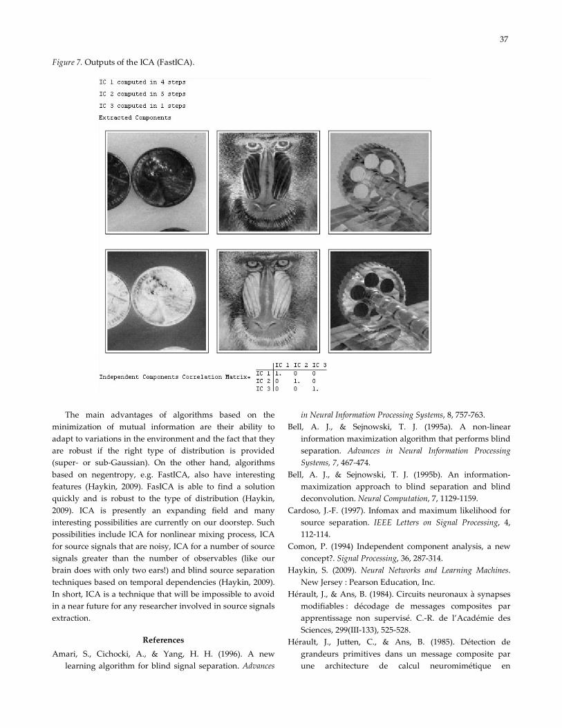
The ICA is then performed (Figure 7). The output of the

Figure 5. Syntax used to load three mixed sources (a) from a file selection window (b).

a)

b)

36

analysis shows the extracted components (in this case,

images) and the correlation matrix of those components.

Since ICA is invariant to the sign of the sources,

extracted components are illustrated using the two possible

signs (background). Finally, a correlation matrix

accompanies the outputs to verify that they are not

correlated.

PCA vs Infomax vs FastICA

The same mixes were used to compare PCA, InfoMax

super (typeOfDist set to super-Gaussian), InfoMax sub

(typeOfDist set to sub-Gaussian), and FastICA. As expected,

PCA and one of the InfoMax analyses (Infomax super) were

unable to find the independent components, since the source

signals used in the example are sub-Gaussian. On the other

hand, InfoMax sub and FastICA performed particularly well

(Figure 8).

Discussion

Readers are encourages to use special softwares that

allow various situations to be taken into account. For

example, FastICA implementations in Matlab, C++, R and

Python can be accessed through the Laboratory of Computer

and Information Science: Adaptive Informatics Research

Center website (http://www.cis.hut.fi/projects/ica/fastica/).

There are also many practical considerations that must be

taken into account that goes beyond the scope of this paper.

For example, it is common practice to pre-whiten the data,

which was done for the FastICA notebook.

Furthermore, many theoretical links can be made

between the different ICA algorithms. For examples,

algorithms that minimize mutual information are linked

together whether they use the Kullback-Leibler divergence

(Amari et al., 1996), maximum likelihood (Pham et al., 1992)

or maximum entropy (Bell & Sejnowski, 1995a; Cardoso,

1997) to do so. Usually, to perform ICA and other blind

source separation problems, five conditions must be met: 1 -

The source signals must be statistically independent; 2 - The

number of source signals must equal the number of mixed

observed signals and mixtures must be linearly independent

from each other; 3 - The model must be noise free; 4 - Data

must be centered and; 5 - The source signals must not have a

Gaussian pdf, except for one single source that can be

Gaussian.

Figure 6. Original signals, mixed signals and mixes correlation matrix for the loaded data.

37

The main advantages of algorithms based on the

minimization of mutual information are their ability to

adapt to variations in the environment and the fact that they

are robust if the right type of distribution is provided

(super- or sub-Gaussian). On the other hand, algorithms

based on negentropy, e.g. FastICA, also have interesting

features (Haykin, 2009). FasICA is able to find a solution

quickly and is robust to the type of distribution (Haykin,

2009). ICA is presently an expanding field and many

interesting possibilities are currently on our doorstep. Such

possibilities include ICA for nonlinear mixing process, ICA

for source signals that are noisy, ICA for a number of source

signals greater than the number of observables (like our

brain does with only two ears!) and blind source separation

techniques based on temporal dependencies (Haykin, 2009).

In short, ICA is a technique that will be impossible to avoid

in a near future for any researcher involved in source signals

extraction.

References

Amari, S., Cichocki, A., & Yang, H. H. (1996). A new

learning algorithm for blind signal separation. Advances

in Neural Information Processing Systems, 8, 757-763.

Bell, A. J., & Sejnowski, T. J. (1995a). A non-linear

information maximization algorithm that performs blind

separation. Advances in Neural Information Processing

Systems, 7, 467-474.

Bell, A. J., & Sejnowski, T. J. (1995b). An information-

maximization approach to blind separation and blind

deconvolution. Neural Computation, 7, 1129-1159.

Cardoso, J.-F. (1997). Infomax and maximum likelihood for

source separation. IEEE Letters on Signal Processing, 4,

112-114.

Comon, P. (1994) Independent component analysis, a new

concept?. Signal Processing, 36, 287-314.

Haykin, S. (2009). Neural Networks and Learning Machines.

New Jersey : Pearson Education, Inc.

Hérault, J., & Ans, B. (1984). Circuits neuronaux à synapses

modifiables : décodage de messages composites par

apprentissage non supervisé. C.-R. de l’Académie des

Sciences, 299(III-133), 525-528.

Hérault, J., Jutten, C., & Ans, B. (1985). Détection de

grandeurs primitives dans un message composite par

une architecture de calcul neuromimétique en

Figure 7. Outputs of the ICA (FastICA).

38

apprentissage non supervisé. Actes du Xème colloque

GRETSI, 1017-1022.

Hyvärinen, A. (1998). New approximations of differential

entropy for independent component analysis and

projection pursuit. Advances in Neural Information

Processing Systems, 10, 273-279.

Hyvärinen, A. (1999a). Survey on Independent Component

Analysis. Neural Computing Surveys, 2, 94-128.

Hyvärinen, A. (1999b). Fast and robust fixed-point

algorithms for independent component analysis. IEEE

Trans. On Neural Networks, 10, 626-634.

Hyvärinen, A., Karhunen, J., & Oja, E. (2001). Independent

Component Analysis. New York : John Wiley & Sons, inc.

Hyvärinen, A., & Oja, E. (2000). Independent component

analysis: algorithms and applications. Neural Networks,

13, 411-430.

Pham, D.-T., Garrat, P. & Jutten, C. (1992). Separation of a

mixture of independent sources through a maximum

likelihood approach. Proceedings EUSIPCO, 771-774.

Manuscript received November 28th, 2009

Manuscript accepted March 30th, 2010.

1 Independent component analysis (ICA) was introduced in

the 80s by J. Hérault, C. Jutten and B. Ans, (Hérault & Ans,

1984; Hérault, Jutten, & Ans, 1985) in the context of studies

on a simplified model of the encoding of movement in

muscle contraction. During that decade, ICA remained

mostly unknown at the international level. In 1994, the name

“independent component analysis” appeared for the first

time in the paper “Independent component analysis, a new

concept?” written by Comon. The technique finally received

attention from a wider portion of the scientific community

with the publication of an ICA algorithm based on the

InfoMax principle (Bell & Sejnowski, 1995a, 1995b). Since

then, ICA has become a well establish area of research in

which many papers, conferences and seminars are now

commonly available. 2 However, this requirement can be relaxed (see for example

Hyvärinen & Oja, 2000). 3 The observation vector must be linearly transformed so

that the correlation matrix gives: .

Figure 8. Outputs from PCA, ICA (InfoMax super), ICA (InfoMax sub) and FastICA.

PCA InfoMax super InfoMax sub FastICA

Extracted component 1

Extracted component 2

Extracted component 3